PRECONDITIONED CONJUGATE GRADIENT METHOD … · PRECONDITIONED CONJUGATE GRADIENT METHOD FOR...

PRECONDITIONED CONJUGATE GRADIENT METHOD FOROPTIMAL CONTROL PROBLEMS WITH CONTROL AND STATE

CONSTRAINTS

ROLAND HERZOG∗ AND EKKEHARD SACHS†

Abstract. Optimality systems and their linearizations arising in optimal control of partialdifferential equations with pointwise control and (regularized) state constraints are considered. Thepreconditioned conjugate gradient (pcg) method in a non-standard inner product is employed fortheir efficient solution. Preconditioned condition numbers are estimated for problems with pointwisecontrol constraints, mixed control-state constraints, and of Moreau-Yosida penalty type. Numericalresults for elliptic problems demonstrate the performance of the pcg iteration. Regularized state-constrained problems in 3D with more than 750,000 variables are solved.

Key words. preconditioned conjugate gradient method, saddle point problems, optimal controlof PDEs, control and state constraints, multigrid method

AMS subject classifications. 49K20, 49M15, 65F08, 65N55

1. Introduction. In their seminal paper [4], Bramble and Pasciak introducedthe idea of applying the preconditioned conjugate gradient (pcg) iteration to symmet-ric indefinite saddle point problems(

A B>

B 0

)(xq

)=

(fg

), (1.1)

where A is a real, symmetric and positive definite matrix, and B is a real m-by-nmatrix with full rank m ≤ n. The application of the pcg iteration becomes possiblethrough the clever use of a suitable scalar product, which renders the preconditionedsaddle point matrix symmetric and positive definite. Meanwhile, this approach hasbeen further developed and it has become a wide spread technique for solving partialdifferential equations (PDEs) in mixed formulation. Very often in these applications,A is positive definite on the whole space.

Recently, Schoberl and Zulehner [19] proposed a symmetric indefinite precondi-tioner with the above properties for the case that A is positive definite only on thenullspace of B:

x>Ax > 0 for all x ∈ kerB \ 0.

This situation is natural when (1.1) is viewed as the first order optimality system ofthe optimization problem

Minimize 1/2x>Ax− f>x s.t. B x = g.

In fact, the authors in [19] show the applicability of their approach to discretizedoptimal control problems for elliptic PDEs with no further constraints. In this paper,we extend their technique to optimal control problems with PDEs in the presence ofcontrol and state constraints, which are usually present in practical examples.

Since even linear inequality constraints give rise to nonlinear optimality systems,we apply a Newton type approach for their solution. Every Newton step is a saddle

∗Chemnitz University of Technology, Faculty of Mathematics, D–09107 Chemnitz, Germany([email protected]).†Department of Mathematics, University of Trier, D–54286 Trier, Germany ([email protected])

1

2 R. HERZOG AND E. SACHS

point problem of type (1.1). Our focus is on the efficient solution of these linearsystems. Therefore we address a key component present in practically every algorithmfor the solution of constrained optimal control problems. We efficiently solve theunderlying linear systems by employing a non-standard inner product preconditionedconjugate gradient method.

Following [19], the building blocks of the preconditioner are preconditioners forthose matrices which represent the scalar products in the spaces X and Q, in which theunknowns x and q are sought. In the context of constrained optimal control problems,x represents the state and control variables, and q comprises the adjoint state andadditional Lagrange multipliers. Optimal preconditioners for scalar product matricesare readily available, e.g., using multigrid or domain decomposition approaches. Dueto their linear complexity and grid independent spectral qualities, the pcg solveralso becomes grid independent and has linear complexity in the number of variables.We use elliptic optimal control problems as examples and proof of concept, but theextension to time dependent problems is straightforward.

The efficient solution of saddle point problems is of paramount importance insolving large scale optimization problems and it is receiving an increasing amount ofattention. Let us put our work into perspective. Various preconditioned Krylov sub-space methods for an accelerated solution of optimality systems in PDE-constrainedoptimization are considered in [1–3,12,14,15]. None of these employ conjugate gradi-ent iterations to the system (1.1). The class of constraint preconditioners approximateonly A in (1.1) and are often applied within a projected preconditioned conjugategradient (ppcg) method. However, preconditioners of this type frequently requirethe inversion of B1 in a partition B = [B1, B2], see [7, 8]. In the context of PDE-constrained optimization, this amounts to the inversion of the PDE operator, whichshould be avoided. Recently, in [17] approximate constraint preconditioners for ppcgiterations are considered in the context of optimal control. It seems, however, thattheir approach lacks extensions to situations where the control acts only on part of thedomain, or on its boundary. An approach similar to ours is presented in [18], where anon-standard inner product conjugate gradient iteration with a block triangular pre-conditioner is devised and applied to an optimal control problem without inequalityconstraints. However, positive definiteness of the (1,1) block is required, which failsto hold, for instance, as soon as the observation of the state variable in the objectiveis reduced to a subdomain. The technique considered here does not have these limita-tions. Finally, we mention [6] where a number of existing approaches is interpreted inthe framework of preconditioned conjugate gradient iterations in non-standard innerproducts.

In the present paper, we apply preconditioned conjugate gradient iterations in anon-standard scalar product to optimal control problems with control and regularizedstate constraints. Through a comparison of the preconditioned condition numbers,we find the Moreau-Yosida penalty approach preferable to regularization by mixedcontrol-state constraints. This is confirmed by numerical results.

The solution of state-constrained problems in 3D is considered computation-ally challenging, and numerical results can hardly be found in the literature. UsingMoreau-Yosida regularization and preconditioned conjugate gradient iterations, theapproach presented here pushes the frontier towards larger problems. The largest3D problem solved has 250,000 state variables, and the same number of control andadjoint state variables, plus Lagrange multipliers. Hence the overall size of the opti-mality system exceeds 750,000.

PCG METHOD FOR OPTIMAL CONTROL PROBLEMS WITH CONSTRAINTS 3

The plan of the paper is as follows. The remainder of this section contains thestanding assumptions. The preconditioned conjugate gradient method is describedin Section 2. We also briefly recall the main results from [19] there. In Section 3,we address its application to the Newton system arising in elliptic optimal controlproblems. We distinguish problems with pointwise control constraints and regular-ized state constraints by way of mixed control-state constraints and a Moreau-Yosidatype penalty approach. Extensive numerical examples are provided in Section 4.Concluding remarks follow in Section 5.

Assumptions. We represent (1.1) in terms of the underlying bilinear forms:Find x ∈ X and q ∈ Q satisfying

a(x,w) + b(w, q) = 〈F,w〉 for all w ∈ Xb(x, r) = 〈G, r〉 for all r ∈ Q,

(1.2)

where X and Q are real Hilbert spaces. The following conditions are well known tobe sufficient to ensure the existence and uniqueness of a solution (x, q) ∈ X ×Q:

1. a is bounded:

a(x,w) ≤ ‖a‖ ‖x‖X ‖w‖X for all x,w ∈ X (1.3a)

2. a is coercive on kerB = x ∈ X : b(x, r) = 0 for all r ∈ Q: There existsα0 > 0 such that

a(x, x) ≥ α0‖x‖2X for all x ∈ kerB (1.3b)

3. b is bounded:

b(x, r) ≤ ‖b‖ ‖x‖X‖r‖Q for all x ∈ X, r ∈ Q (1.3c)

4. b satisfies the inf–sup condition: There exists k0 > 0 such that

supx∈X

b(x, r) ≥ k0 ‖x‖X‖r‖Q for all r ∈ Q. (1.3d)

5. a is symmetric and non-negative, i.e.,

a(x,w) = a(w, x) and a(x, x) ≥ 0 for all x,w ∈ X. (1.3e)

In constrained optimal control applications, x will correspond to the state andcontrol variables, while q comprises the adjoint state and Lagrange multipliers asso-ciated with inequality constraints.

Notation. For symmetric matrices, A B means that B−A is positive semidef-inite, and A ≺ B means that B −A is positive definite.

2. Preconditioned Conjugate Gradient Method. In this section we recallthe main results from [19] and give some algorithmic details concerning the precon-ditioned conjugate gradient iteration. We consider a Galerkin discretization of (1.2)with finite dimensional subspaces Xh ⊂ X and Qh ⊂ Q. Here and throughout, Xand Q are the matrices representing the scalar products in the subspaces Xh and Qh,respectively. Moreover, A and B are the matrices representing the bilinear forms aand b, respectively, with respect to a chosen basis on these subspaces. It is assumed


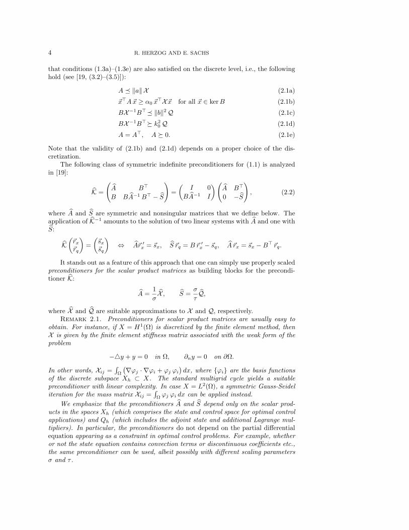
that conditions (1.3a)–(1.3e) are also satisfied on the discrete level, i.e., the followinghold (see [19, (3.2)–(3.5)]):

A ‖a‖X (2.1a)

~x>A~x ≥ α0 ~x>X~x for all ~x ∈ kerB (2.1b)

BX−1B> ‖b‖2Q (2.1c)

BX−1B> k20 Q (2.1d)

A = A>, A 0. (2.1e)

Note that the validity of (2.1b) and (2.1d) depends on a proper choice of the dis-cretization.

The following class of symmetric indefinite preconditioners for (1.1) is analyzedin [19]:

K =

(A B>

B BA−1B> − S

)=

(I 0

BA−1 I

)(A B>

0 −S

), (2.2)

where A and S are symmetric and nonsingular matrices that we define below. Theapplication of K−1 amounts to the solution of two linear systems with A and one withS:

K(~rx~rq

)=

(~sx~sq

)⇔ A~r ′x = ~sx, S ~rq = B~r ′x − ~sq, A ~rx = ~sx −B> ~rq.

It stands out as a feature of this approach that one can simply use properly scaledpreconditioners for the scalar product matrices as building blocks for the precondi-tioner K:

A =1

σX , S =

σ

τQ,

where X and Q are suitable approximations to X and Q, respectively.Remark 2.1. Preconditioners for scalar product matrices are usually easy to

obtain. For instance, if X = H1(Ω) is discretized by the finite element method, thenX is given by the finite element stiffness matrix associated with the weak form of theproblem

−4y + y = 0 in Ω, ∂ny = 0 on ∂Ω.

In other words, Xij =∫

Ω

(∇ϕj · ∇ϕi + ϕj ϕi

)dx, where ϕi are the basis functions

of the discrete subspace Xh ⊂ X. The standard multigrid cycle yields a suitablepreconditioner with linear complexity. In case X = L2(Ω), a symmetric Gauss-Seideliteration for the mass matrix Xij =

∫Ωϕj ϕi dx can be applied instead.

We emphasize that the preconditioners A and S depend only on the scalar prod-ucts in the spaces Xh (which comprises the state and control space for optimal controlapplications) and Qh (which includes the adjoint state and additional Lagrange mul-tipliers). In particular, the preconditioners do not depend on the partial differentialequation appearing as a constraint in optimal control problems. For example, whetheror not the state equation contains convection terms or discontinuous coefficients etc.,the same preconditioner can be used, albeit possibly with different scaling parametersσ and τ .


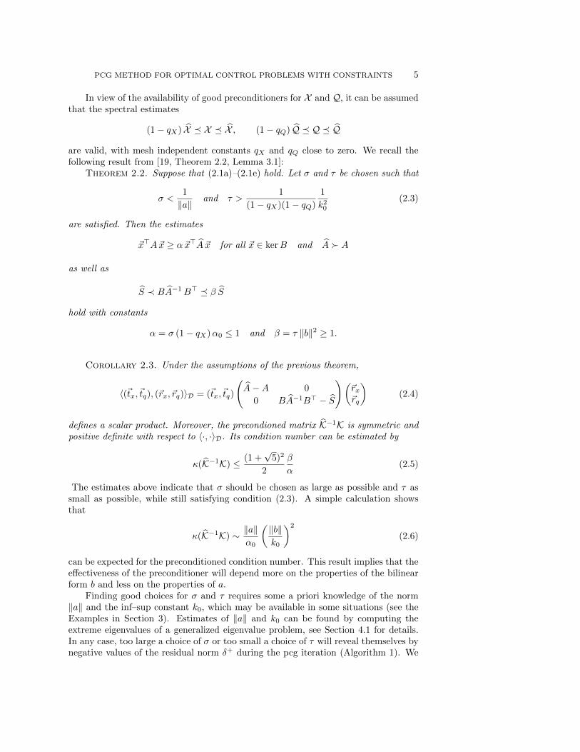
In view of the availability of good preconditioners for X and Q, it can be assumedthat the spectral estimates

(1− qX) X X X , (1− qQ) Q Q Q

are valid, with mesh independent constants qX and qQ close to zero. We recall thefollowing result from [19, Theorem 2.2, Lemma 3.1]:

Theorem 2.2. Suppose that (2.1a)–(2.1e) hold. Let σ and τ be chosen such that

σ <1

‖a‖and τ >

1

(1− qX)(1− qQ)

1

k20

(2.3)

are satisfied. Then the estimates

~x>A~x ≥ α~x>A ~x for all ~x ∈ kerB and A A

as well as

S ≺ BA−1B> β S

hold with constants

α = σ (1− qX)α0 ≤ 1 and β = τ ‖b‖2 ≥ 1.

Corollary 2.3. Under the assumptions of the previous theorem,

〈(~tx,~tq), (~rx, ~rq)〉D = (~tx,~tq)

(A−A 0

0 BA−1B> − S

)(~rx~rq

)(2.4)

defines a scalar product. Moreover, the precondioned matrix K−1K is symmetric andpositive definite with respect to 〈·, ·〉D. Its condition number can be estimated by

κ(K−1K) ≤ (1 +√

5)2

2

β

α(2.5)

The estimates above indicate that σ should be chosen as large as possible and τ assmall as possible, while still satisfying condition (2.3). A simple calculation showsthat

κ(K−1K) ∼ ‖a‖α0

(‖b‖k0

)2

(2.6)

can be expected for the preconditioned condition number. This result implies that theeffectiveness of the preconditioner will depend more on the properties of the bilinearform b and less on the properties of a.

Finding good choices for σ and τ requires some a priori knowledge of the norm‖a‖ and the inf–sup constant k0, which may be available in some situations (see theExamples in Section 3). Estimates of ‖a‖ and k0 can be found by computing theextreme eigenvalues of a generalized eigenvalue problem, see Section 4.1 for details.In any case, too large a choice of σ or too small a choice of τ will reveal themselves bynegative values of the residual norm δ+ during the pcg iteration (Algorithm 1). We


thus employ a simple safeguard strategy (Algorithm 2) to correct unsuitable scalingparameters.

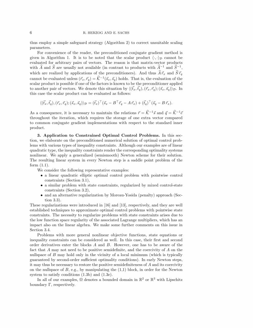
For convenience of the reader, the preconditioned conjugate gradient method isgiven in Algorithm 1. It is to be noted that the scalar product 〈·, ·〉D cannot beevaluated for arbitrary pairs of vectors. The reason is that matrix-vector productswith A and S are usually not available (in contrast to products with A−1 and S−1,

which are realized by applications of the preconditioners). And thus A ~rx and S ~rqcannot be evaluated unless (~rx, ~rq) = K−1(~sx, ~sq) holds. That is, the evaluation of thescalar product is possible if one of the factors is known to be the preconditioner appliedto another pair of vectors. We denote this situation by 〈(~tx,~tq), (~rx, ~rq); (~sx, ~sq)〉D. Inthis case the scalar product can be evaluated as follows:

〈(~tx,~tq), (~rx, ~rq); (~sx, ~sq)〉D = (~tx)>(~sx −B>~rq −A~rx) + (~tq)>(~sq −B~rx).

As a consequence, it is necessary to maintain the relations ~r = K−1~s and ~q = K−1~ethroughout the iteration, which requires the storage of one extra vector comparedto common conjugate gradient implementations with respect to the standard innerproduct.

3. Application to Constrained Optimal Control Problems. In this sec-tion, we elaborate on the preconditioned numerical solution of optimal control prob-lems with various types of inequality constraints. Although our examples are of linearquadratic type, the inequality constraints render the corresponding optimality systemsnonlinear. We apply a generalized (semismooth) Newton scheme for their solution.The resulting linear system in every Newton step is a saddle point problem of theform (1.1).

We consider the following representative examples:• a linear quadratic elliptic optimal control problem with pointwise control

constraints (Section 3.1),• a similar problem with state constraints, regularized by mixed control-state

constraints (Section 3.2),• and an alternative regularization by Moreau-Yosida (penalty) approach (Sec-

tion 3.3).These regularizations were introduced in [16] and [13], respectively, and they are wellestablished techniques to approximate optimal control problems with pointwise stateconstraints. The necessity to regularize problems with state constraints arises due tothe low function space regularity of the associated Lagrange multipliers, which has animpact also on the linear algebra. We make some further comments on this issue inSection 3.4.

Problems with more general nonlinear objective functions, state equations orinequality constraints can be considered as well. In this case, their first and secondorder derivatives enter the blocks A and B. However, one has to be aware of thefact that A may not need to be positive semidefinite, and the coercivity of A on thenullspace of B may hold only in the vicinity of a local minimum (which is typicallyguaranteed by second-order sufficient optimality conditions). In early Newton steps,it may thus be necessary to restore the positive semidefiniteness of A and its coercivityon the nullspace of B, e.g., by manipulating the (1,1) block, in order for the Newtonsystem to satisfy conditions (1.3b) and (1.3e).

In all of our examples, Ω denotes a bounded domain in R2 or R3 with Lipschitzboundary Γ, respectively.


Algorithm 1 Conjugate gradient method for K−1K w.r.t. to scalar product D.

Input: right hand side (~bx,~bq) and initial iterate (~xx, ~xq)

Output: solution (~xx, ~xq) of K (~xx, ~xq) = (~bx,~bq)1: Set n := 0 and compute initial residual(

~sx~sq

):=

(~bx −A~xx −B>~xq

~bq −B ~xx

)and

(~dx~dq

):=

(~rx~rq

):= K−1

(~sx~sq

)2: Set δ0 := δ+ := 〈(~rx, ~rq), (~rx, ~rq); (~sx, ~sq)〉D3: while n < nmax and δ+ > ε2

rel δ0 and δ+ > ε2abs do

4: Set (~ex~eq

):=

(A ~dx +B>~dq

B ~dx

)and

(~qx~qq

):= K−1

(~ex~eq

)

5: Set α := δ+/〈(~dx, ~dq), (~qx, ~qq); (~ex, ~eq)〉D6: Update the solution (

~xx~xq

):=

(~xx~xq

)+ α

(~dx~dq

)

7: Update the residual(~rx~rq

):=

(~rx~rq

)− α

(~qx~qq

)and

(~sx~sq

):=

(~sx~sq

)− α

(~ex~eq

)8: Set δ := δ+ and δ+ := 〈(~rx, ~rq), (~rx, ~rq); (~sx, ~sq)〉D9: Set β := δ+/δ

10: Update the search direction(~dx~dq

):=

(~rx~rq

)+ β

(~dx~dq

)

11: Set n := n+ 112: end while13: return (~xx, ~xq)

Algorithm 2 Safeguard strategy for selection of scaling parameters σ, τ .

1: Determine an underestimate ‖a‖′ ≤ ‖a‖ and an overestimate k′0 ≥ k0

2: Set σ = 0.9/‖a‖′ and τ = 1.2/(k′0)2 and scaling rejected := true

3: while scaling rejected do4: Run the pcg iteration (Algorithm 1)5: if it fails with δ+ < 0 then6: Set σ := σ/

√2 and τ :=

√2 τ

7: else8: Set scaling rejected := false

9: end if10: end while


3.1. Control Constraints. We consider the following optimal control problemwith pointwise control constraints:

Minimize1

2‖y − yd‖2L2(Ω) +

ν

2‖u‖2L2(Ω)

s.t.

−4y + y = u in Ω

∂ny = 0 on Γ

and ua ≤ u ≤ ub a.e. in Ω.

(CC)

Here, ν > 0 denotes the control cost parameter, ∂n is the normal derivative on theboundary, and ua and ub are the lower and upper bounds for the control variable u.The first order system of necessary and sufficient optimality conditions of (CC) canbe expressed as follows (compare [21, Section 2.8.2]):

−4p+ p = −(y − yd) in Ω, ∂np = 0 on Γ (3.1a)

ν u− p+ ξ = 0 a.e. in Ω (3.1b)

−4y + y = u in Ω, ∂ny = 0 on Γ (3.1c)

ξ −max0, ξ + c (u− ub) −min0, ξ − c (ua − u) = 0 a.e. in Ω (3.1d)

for any c > 0. In (3.1), p denotes the adjoint state, and ξ is the Lagrange multiplierassociated to the control constraints. Note that eq. (3.1d) is equivalent to the twopointwise complementarity systems

0 ≤ ξ+, u− ub ≤ 0, ξ+(u− ub) = 0

0 ≤ ξ−, ua − u ≤ 0, ξ−(ua − u) = 0.

It is well known that (3.1) enjoys the Newton differentiability property [11], atleast for c = ν. Hence, a generalized (semismooth) Newton iteration can be applied.We focus on the preconditioned solution of the generalized Newton steps. Due tothe structure of the nonsmooth part (3.1d), the Newton iteration can be expressedin terms of an active set strategy. Given an iterate (yk, uk, pk, ξk), the active sets aredetermined by

A+k = x ∈ Ω : ξk + c (uk − ub) > 0A−k = x ∈ Ω : ξk − c (ua − uk) < 0,

(3.2)

and the inactive set is Ik = Ω\ (A+k ∪A

−k ). The Newton step for the solution of (3.1),

given in terms of the new iterate, reads as follows:I · L∗ ·· ν I −I IL −I · ·· c χAk

· χIk

yk+1

uk+1

pk+1

ξk+1

=

yd00

c(χA+

kub + χA−k

ua) , (3.3)

where χA+k

, χA−kand χAk

denote the characteristic functions of A+k , A−k and Ak =

A+k ∪A

−k , respectively, and L represents the differential operator of the PDE constraint

in (CC). In the present example, we have L = −4+ I with homogeneous Neumannboundary conditions in weak form, considered as an operator fromH1(Ω) intoH1(Ω)∗.We emphasize that the Newton system (3.3) changes from iteration to iteration due


to changes in the active sets. Since, however, we focus here on the efficient solutionof individual Newton steps, we drop the iteration index from now on.

From (3.3) one infers ξI = 0 (the restriction of ξ to the inactive set I), andwe eliminate this variable from the problem. The Newton system then attains anequivalent symmetric saddle point form:

I · L∗ ·· ν I −I χAL −I · ·· χA · ·

yupξA

=

yd00

χA+ ub + χA− ua

, (3.4)

which fits into our framework (1.2) with the following identifications

x = (y, u) ∈ X = H1(Ω)× L2(Ω)

q = (p, ξA) ∈ Q = H1(Ω)× L2(A)

and bilinear forms

a((y, u), (z, v)

):= (y, z)L2(Ω) + ν (u, v)L2(Ω) (3.5a)

b((y, u), (p, ξA)

):= (y, p)H1(Ω) − (u, p)L2(Ω) + (u, ξA)L2(A). (3.5b)

Lemma 3.1. The bilinear forms a(·, ·) and b(·, ·) satisfy the assumptions (1.3a)–(1.3e) with constants ‖a‖ = max1, ν, α0 = ν/2, ‖b‖ = 2, and k0 = 1/2, independentof the active set A.

Proof. The proof uses the Cauchy-Schwarz and Young’s inequalities. The bound-edness of a follows from

a((y, u), (z, v)

)≤ ‖y‖L2(Ω)‖z‖L2(Ω) + ν ‖u‖L2(Ω)‖v‖L2(Ω)

≤(‖y‖2L2(Ω) + ν ‖u‖2L2(Ω)

)1/2(‖z‖2L2(Ω) + ν ‖v‖2L2(Ω)

)1/2≤ max1, ν‖(y, u)‖X‖(z, v)‖X .

To verify the coervity of a, let (y, u) ∈ kerB. Then in particular, (y, p)H1(Ω) =(u, p)L2(Ω) holds for all p ∈ H1(Ω), and from p = y we obtain the a priori estimate‖y‖H1(Ω) ≤ ‖u‖L2(Ω). This implies

a((y, u), (y, u)

)= ‖y‖2L2(Ω) + ν ‖u‖2L2(Ω)

≥ ν

2‖y‖2H1(Ω) +

ν

2‖u‖2L2(Ω) =

ν

2‖(y, u)‖2X .

The boundedness of b follows from

b((y, u), (p, ξA)

)≤ ‖y‖H1(Ω)‖p‖H1(Ω) + ‖u‖L2(Ω)‖p‖L2(Ω) + ‖u‖L2(A)‖ξ‖L2(A)

≤(‖y‖H1(Ω) + ‖u‖L2(Ω)

)(‖p‖H1(Ω) + ‖ξ‖L2(A)

)≤ 2 ‖(y, u)‖X‖(p, ξA)‖Q.

Finally, we obtain the inf–sup condition for b as follows: For given (p, ξA) ∈ Q, choose


y = p and u = ξA (by extending it by zero outside of A). Then

b((y, u), (p, ξA)

)≥ ‖p‖2H1(Ω) − ‖ξA‖L2(Ω)‖p‖L2(Ω) + ‖ξA‖2L2(A)

≥ ‖p‖2H1(Ω) −1

2‖ξA‖2L2(Ω) −

1

2‖p‖2L2(Ω) + ‖ξA‖2L2(A)

≥ 1

2‖p‖2H1(Ω) +

1

2‖ξA‖2L2(A)

=1

2

(‖y‖2H1(Ω) + ‖u‖2L2(Ω)

)1/2(‖p‖2H1(Ω) + ‖ξA‖2L2(Ω)

)1/2=

1

2‖(y, u)‖X‖(p, ξA)‖Q.

The leading term in the estimate for the preconditioned condition number, see (2.5)and (2.6), is thus

κCC(K−1K) ∼ β

α= 32 ν−1 max1, ν.

Remark 3.2. The treatment of an additional term γ ‖u‖L1(Ω) in the objective of(CC) is easily possible. For positive γ, this term promotes so-called sparse optimalcontrols, which are zero on non-trivial parts of the domain. The corresponding opti-mality system can be found in [20, Lemma 2.2]. The Newton iteration for the solutionof this extended problem requires two changes: Firstly, the active sets are determinedfrom

A+ = x ∈ Ω : ξ − γ + c (u− ub) > 0A− = x ∈ Ω : ξ + γ − c (ua − u) < 0A0 = x ∈ Ω : −ξ − γ ≤ c u ≤ −ξ + γ,

and A := A+ ∪ A− ∪ A0. Note that A0 is the set where the updated control iszero. Secondly, at the end of each Newton step, ξI is updated according to ξI =χI+ γ−χI− γ, where I+ is the subset of Ω where c u+ ξ−γ is between 0 and ub, andsimilarly for I−.

In particular, the Newton system (3.4) remains the same, and thus problems withan additional sparsity term can be solved just as efficiently as problems with controlconstraints alone.

Discretization. We now turn to the discretization of (CC) and the Newton step(3.4) by a Galerkin method. We introduce

Mh = (ϕi, ϕj)L2(Ω) mass matrix (3.6a)

Lh = Kh = (∇ϕi,∇ϕj)L2(Ω) + (ϕi, ϕj)L2(Ω) stiffness matrix, (3.6b)

where ϕini=1 is a basis of a discrete subspace of H1(Ω). The coordinate vector of yw.r.t. this basis is denoted by ~y. Here and throughout, Lh corresponds to the differ-ential operator, and Kh represents the scalar product in the state space H1(Ω). Forsimplicity, we discretize all variables by piecewise linear Lagrangian finite elements.A straightforward modification would allow a different discretization of the controlspace, e.g., by piecewise constants.


The discrete counterpart of (CC) is

Minimize1

2(~y − ~yd)>Mh(~y − ~yd) +

ν

2~u>Mh~u

s.t. Lh~y −Mh~u = ~0

and ~ua ≤ ~u ≤ ~ub.

(CCh)

Its optimality conditions are a discrete variant of (3.1):

L>h ~p = −Mh(~y − ~yd) (3.7a)

ν Mh~u−Mh~p+ ~µ = 0 (3.7b)

Lh~y = Mh~u (3.7c)

~µ−max0, ~µ+ c (~u− ~ub) −min0, ~µ− c (~ua − ~u) = 0, (3.7d)

and a Newton step applied to (3.7) leads to the following discrete linear system:Mh · L>h ·· ν Mh −Mh ILh −Mh · ·· c χA · χI

~y~u~p~µ

=

Mh~yd

00

c(χA+ ~ub + χA− ~ua

) .

On the discrete level, χA is a diagonal 0-1-matrix. As in the continuous setting, weinfer ~µI = ~0 and eliminate this variable to obtain

Mh · L>h ·· ν Mh −Mh P>ALh −Mh · ·· PA · ·

~y~u~p~µA

=

Mh~yd

00

PA+ ~ub + PA− ~ua

. (3.8)

PA is a rectangular matrix consisting of those rows of χA which belong to the activeindices, and similarly for PA± .

Some comments concerning the discrete system (3.8) are in order. The variable~µ is the Lagrange multiplier associated to the discrete constraint ~ua ≤ ~u ≤ ~ub, andthe relations ~µ = P>A ~µA and ~µA = PA ~µ hold. If we set ~ξ = M−1

h ~µ, then ~ξ is thecoordinate vector of a function in L2(Ω) which approximates the multiplier ξ in thecontinuous system (3.1d). This observation is reflected by the choice of norms on thediscrete level, see (3.9) below.

With the settings

~x = (~y, ~u) ∈ Xh = Rn × Rn

~q = (~p, ~µA) ∈ Qh = Rn × RnA

and bilinear forms

ah((~y, ~u), (~z,~v)

):= ~z>Mh~y + ν ~v>Mh~u

bh((~y, ~u), (~p, ~µA)

):= ~p>Lh~y − ~p>Mh~u+ ~µ>A(PA~u)

the discrete problem fits into the framework (1.2). As mentioned above, care has to betaken in choosing an appropriate norm for the discrete multiplier ~µA. We use scalarproducts in the spaces Xh and Qh represented by the following matrices:

X =

(Kh

Mh

)and Q =

(Kh

P>AM−1h PA

)(3.9)


with Mh and Kh defined in (3.6).Due to the use of a conforming Galerkin approach, the constants ‖a‖ and ‖b‖ on

the discrete level are the same as in Lemma 3.1 above, and, in particular, they areindependent of the mesh size h. The same can be shown for α0 and k0.

Note that the equation PAM−1h P>A ~µA = ~bA is equivalent to the linear system(

Mh P>APA 0

)(~r~µA

)= −

(~0~bA

). (3.10)

This fact is exploited in the construction of the preconditioner below.

Preconditioner. We recall that the preconditioner has the form

K =

(I 0

BA−1 I

)(A B>

0 −S

)

and that the framework of [19] solely requires correctly scaled preconditioners for thescalar product matrices defined in (3.9). We use

A =1

σ

(Kh

Mh

)and S =

σ

τ

(Kh

PAM−1h P>A

)(3.11)

with scaling parameters

σ = 0.9/‖a‖, τ = 1.2/k20

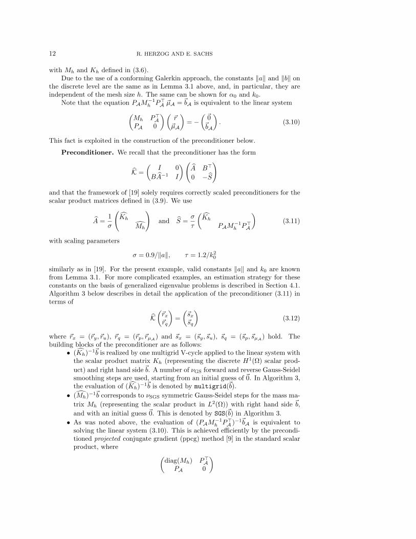
similarly as in [19]. For the present example, valid constants ‖a‖ and k0 are knownfrom Lemma 3.1. For more complicated examples, an estimation strategy for theseconstants on the basis of generalized eigenvalue problems is described in Section 4.1.Algorithm 3 below describes in detail the application of the preconditioner (3.11) interms of

K(~rx~rq

)=

(~sx~sq

)(3.12)

where ~rx = (~ry, ~ru), ~rq = (~rp, ~rµA) and ~sx = (~sy, ~su), ~sq = (~sp, ~sµA) hold. Thebuilding blocks of the preconditioner are as follows:

• (Kh)−1~b is realized by one multigrid V-cycle applied to the linear system withthe scalar product matrix Kh (representing the discrete H1(Ω) scalar prod-

uct) and right hand side~b. A number of νGS forward and reverse Gauss-Seidelsmoothing steps are used, starting from an initial guess of ~0. In Algorithm 3,the evaluation of (Kh)−1~b is denoted by multigrid(~b).

• (Mh)−1~b corresponds to νSGS symmetric Gauss-Seidel steps for the mass ma-

trix Mh (representing the scalar product in L2(Ω)) with right hand side ~b,

and with an initial guess ~0. This is denoted by SGS(~b) in Algorithm 3.

• As was noted above, the evaluation of (PAM−1h P>A )−1~bA is equivalent to

solving the linear system (3.10). This is achieved efficiently by the precondi-tioned projected conjugate gradient (ppcg) method [9] in the standard scalarproduct, where (

diag(Mh) P>APA 0

)


serves as a preconditioner. In Algorithm 3, this corresponds to the callppcg(~bA,A+,A−). In practice, we use a relative termination tolerance of10−12 for the residual in ppcg, which took at most 13 steps to converge inall examples. The reason for solving (3.10) practically to convergence is thatintermediate iterates in conjugate gradient iterations depend nonlinearly onthe right hand side, and thus early termination would yield a nonlinear pre-conditioner S. Note that the projected conjugated gradient method requiresan initial iterate consistent with the second equation PA ~r = −~bA in (3.10).

Due to the structure of PA, we can simply use ~rA = −~bA, ~rI = ~0 and ~µA = ~0as initial iterate.

Before moving on to problems with different types of constraints, we briefly sum-marize the main features of the pcg iteration applied to the solution of the Newtonstep (3.8).

Remark 3.3.1. The main effort in every application of the preconditioner are the three multi-

grid cycles. No partial differential equations need to be solved. Moreover, themethod is of linear complexity in the number of unknowns.

2. In the case, where the control u and thus the Lagrange multiplier ξ are dis-cretized by piecewise constant functions, the mass matrix Mh in the scalarproduct X becomes a diagonal matrix, and preconditioning for the blocks Mh

and PAM−1h P>A becomes trivial.

3. We recall that the matrix B in Algorithm 3 denotes the (2,1) block of (3.8),i.e.,

B =

(Lh −Mh

· PA

)in the control-constrained case presently considered. For the subsequent ex-amples, B changes, but no other modifications to Algorithm 3 are required.

Algorithm 3 Application of the preconditioner according to (3.12)

Input: right hand sides ~sx = (~sy, ~su) and ~sq = (~sp, ~sµA), scaling parameters σ, τ , andactive sets A+,A−

Output: solution ~rx = (~ry, ~ru) and ~rq = (~rp, ~rµA) of (3.12)

1: ~r ′y := multigrid(σ ~sy)

2: ~r ′~u := SGS(σ ~su)

3:

(~s ′p~s ′µA

):= B

(~r ′y~r ′u

)−(~sp~sµA

)4: ~rp := multigrid(τ ~s ′p/σ)

5: ~rµA := ppcg(τ ~s ′µA/σ,A+,A−)

6:

(~s ′y~s ′u

):=

(~sy~su

)−B>

(~rp~rµA

)7: ~ry := multigrid(σ ~s ′y)

8: ~ru := SGS(σ ~s ′u)

9: return ~ry, ~ru, ~rp, ~rµA


3.2. Regularized State-Constrained Problems: Mixed Constraints. Inthis section we address optimal control problems with mixed control-state constraints.They can be viewed as one way of regularizing problems with pure state constraints,see [16]:

Minimize1

2‖y − yd‖2L2(Ω) +

ν

2‖u‖2L2(Ω)

s.t.

−4y + y = u in Ω

∂ny = 0 on Γ

and ya ≤ ε u+ y ≤ yb a.e. in Ω.

(MC)

We point out the main differences to the control constrained case. The first ordersystem of necessary and sufficient optimality conditions of (MC) can be expressed asfollows:

−4p+ p = −(y − yd)− ξ in Ω, ∂np = 0 on Γ (3.13a)

ν u− p+ ε ξ = 0 a.e. in Ω (3.13b)

−4y + y = u in Ω, ∂ny = 0 on Γ (3.13c)

ξ −max0, ξ + c (ε u+ y − yb) −min0, ξ − c (ya − ε u− y) = 0 a.e. in Ω.(3.13d)

A Newton step for the solution of (3.13) reads (in its symmetric form)I · L∗ χA· ν I −I ε χAL −I · ·χA ε χA · ·

yupξA

=

yd00

χA+ yb + χA− ya

with active sets similar as in (3.2). The Newton system fits into our framework (1.2)with the following identifications

x = (y, u) ∈ X = H1(Ω)× L2(Ω)

q = (p, ξA) ∈ Q = H1(Ω)× L2(A)

and bilinear forms

a((y, u), (z, v)

):= (y, z)L2(Ω) + ν (u, v)L2(Ω)

b((y, u), (p, ξA)

):= (y, p)H1(Ω) − (u, p)L2(Ω) + (y, ξA)L2(A) + ε (u, ξA)L2(A).

Lemma 3.4. The bilinear forms a(·, ·) and b(·, ·) satisfy the assumptions (1.3a)–(1.3e) with constants ‖a‖ = max1, ν, α0 = ν/2, ‖b‖ = 2 max1, ε, and k0 =min1, ε, independent of the active set A.

Proof. The bilinear form a is the same as in (3.5a), hence we refer to the proof ofLemma 3.1 for ‖a‖ and α0. (Although kerB has changed, we used only the conditionLy − u = 0 in the proof of Lemma 3.1, which remains valid.) The boundedness of bfollows from

b((y, u), (p, ξA)

)≤ ‖y‖H1(Ω)‖p‖H1(Ω) + ‖u‖L2(Ω)‖p‖L2(Ω) + ‖y‖L2(A)‖ξA‖L2(A)

+ ε ‖u‖L2(A)‖ξA‖L2(A)

≤(‖y‖H1(Ω) + max1, ε ‖u‖L2(Ω)

)(‖p‖H1(Ω) + ‖ξA‖L2(A)

)≤ 2 max1, ε ‖(y, u)‖X‖(p, ξA)‖Q.


Finally, we obtain the inf–sup condition for b as follows: For given (p, ξA) ∈ Q, choosey = p and u = ξA (by extending it by zero outside of A). Then

b((y, u), (p, ξA)

)= (p, p)H1(Ω) − (ξA, p)L2(Ω) + (p, ξA)L2(A) + ε (ξA, ξA)L2(A)

≥ ‖p‖2H1(Ω) + ε ‖ξA‖2L2(A)

≥ min1, ε‖(y, u)‖X‖(p, ξA)‖Q.

The leading term in the estimate for the preconditioned condition number is thus

κMC(K−1K) ∼ β

α= 8

max1, νν

(max1, εmin1, ε

)2

,

which scales like ε−2 for small ε.

Discretization. The discretization is carried out like in Section 3.1. The discreteNewton step becomes

Mh · L>h P>A· ν Mh −Mh ε P>ALh −Mh · ·PA ε PA · ·

~y~u~p~µA

=

Mh~yd

00

PA+ ~yb + PA− ~ya

.

The scalar products and thus the preconditioner are the same (with different constantsσ and τ) as in the control constrained case, Section 3.1. We only point out that now

B =

(Lh −Mh

PA ε PA

)has to be used in Algorithm 3.

3.3. Regularized State-Constrained Problems: Moreau-Yosida Approach.An alternative regularization approach for state constrained problems is given in termsof the Moreau-Yosida penalty function (see [13]):

Minimize1

2‖y − yd‖2L2(Ω) +

ν

2‖u‖2L2(Ω) +

1

2ε‖max0, y − yb‖2L2(Ω)

+1

2ε‖min0, y − ya‖2L2(Ω)

s.t.

−4y + y = u in Ω

∂ny = 0 on Γ.

(MY)

The first order system of necessary and sufficient optimality conditions of (MY) canbe expressed as follows:

−4p+ p = −(y − yd)− ξ in Ω, ∂np = 0 on Γ (3.14a)

ν u− p = 0 a.e. in Ω (3.14b)

−4y + y = u in Ω, ∂ny = 0 on Γ (3.14c)

with the abbreviation ξ = ε−1 max0, y − yb + ε−1 min0, ya − y. A Newton stepfor the solution of (3.14) readsI + χA

ε · L∗

· ν I −IL −I ·

yup

=

yd + 1ε

(χA+ yb + χA− ya

)00


with active sets

A+ = x ∈ Ω : y − yb > 0A− = x ∈ Ω : ya − y < 0.

The variables and bilinear forms are now given by

x = (y, u) ∈ X = H1(Ω)× L2(Ω)

q = p ∈ Q = H1(Ω)

and

a((y, u), (z, v)

):= (y, z)L2(Ω) + ε−1(y, z)L2(A) + ν (u, v)L2(Ω)

b((y, u), p

):= (y, p)H1(Ω) − (u, p)L2(Ω).

Note that in contrast to the mixed constrained approach (Section 3.2), the regu-larization parameter ε now appears in the bilinear form a instead of b.

Lemma 3.5. The bilinear forms a(·, ·) and b(·, ·) satisfy the assumptions (1.3a)–(1.3e) with constants ‖a‖ = max1 + ε−1, ν, α0 = ν/2, ‖b‖ =

√2, and k0 = 1,

independent of the active set A.

The proof is similar to that of Lemma 3.1 and Lemma 3.4 and is therefore omitted.The leading term in the estimate for the preconditioned condition number is now

κMY(K−1K) ∼ β

α= 8

max1 + ε−1, νν

which scales like ε−1 for small ε.

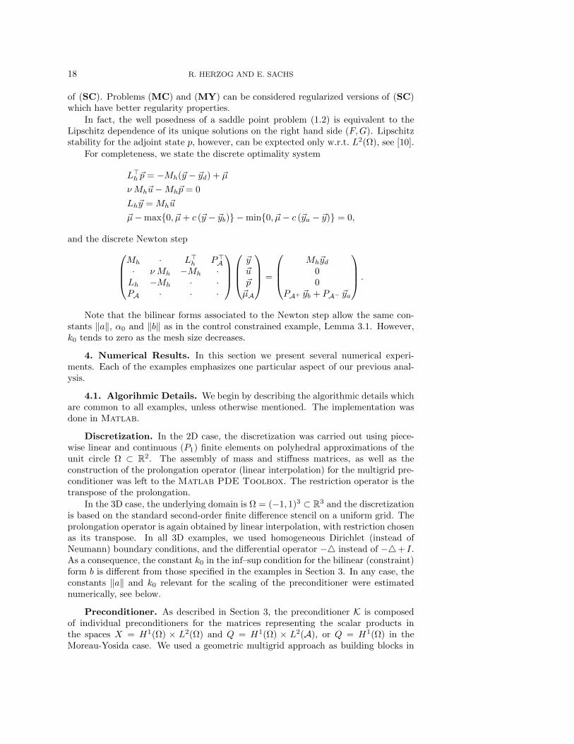
As mentioned before, problems (MC) and (MY) can be viewed as regularized ver-sions of the state constrained problem (SC) below. Provided that the regularizationerrors are comparable for identical values of ε, the estimates for the preconditionedcondition number clearly favor the Moreau-Yosida approach, see Figure 3.1. This isconfirmed by the numerical results in Section 4.

Discretization. The discrete counterpart of (MY) is

Minimize1

2(~y − ~yd)>Mh(~y − ~yd) +

ν

2~u>Mh~u

+1

2εmax0, ~y − ~yb>Mh max0, ~y − ~yb

+1

2εmin0, ~y − ~ya>Mh min0, ~y − ~ya

s.t. Lh~y = Mh~u

(MYh)

and its optimality conditions read

L>h ~p = −Mh(~y − ~yd)− χA+ε−1Mh max0, ~y − ~yb − χA−ε−1Mh min0, ~y − ~ya(3.15a)

ν Mh~u−Mh~p = 0 (3.15b)

Lh~y = Mh~u (3.15c)


where χA+ are the indices where ~y − ~yb > 0 and similarly for χA− . A Newton stepfor (3.15) amounts to solvingMh + χA

ε MhχA · L>h· ν Mh −Mh

Lh −Mh ·

~y~u~p

=

Mh~yd + 1ε

(χA+MhχA+~yb + χA−MhχA−~ya

)00

The preconditioner is the same as described in Algorithm 3, with the exception thatnow

B =(Lh −Mh

)is used, and step 5 can be omitted since no Lagrange multipliers associated to in-equality constraints are present in the Moreau-Yosida case.

Fig. 3.1. Comparison of preconditioned condition numbers for mixed control-state constraints(left) and Moreau-Yosida regularization (right), as functions of the control cost coefficient ν and theregularization parameter ε.

3.4. State-Constrained Problems. We briefly address an optimal controlproblem with pointwise state constraints.

Minimize1

2‖y − yd‖2L2(Ω) +

ν

2‖u‖2L2(Ω)

s.t.

−4y + y = u in Ω

∂ny = 0 on Γ

and ya ≤ y ≤ yb in Ω.

(SC)

It is well known that (SC) does not permit the same function space setting as inthe previous sections. The associated Lagrange multiplier is only a measure [5], andthe adjoint state belongs to W 1,s(Ω) where s < N/(N − 1). Moreover, there is notheoretical foundation of using Newton type methods in function space for the solution


of (SC). Problems (MC) and (MY) can be considered regularized versions of (SC)which have better regularity properties.

In fact, the well posedness of a saddle point problem (1.2) is equivalent to theLipschitz dependence of its unique solutions on the right hand side (F,G). Lipschitzstability for the adjoint state p, however, can be exptected only w.r.t. L2(Ω), see [10].

For completeness, we state the discrete optimality system

L>h ~p = −Mh(~y − ~yd) + ~µ

ν Mh~u−Mh~p = 0

Lh~y = Mh~u

~µ−max0, ~µ+ c (~y − ~yb) −min0, ~µ− c (~ya − ~y) = 0,

and the discrete Newton stepMh · L>h P>A· ν Mh −Mh ·Lh −Mh · ·PA · · ·

~y~u~p~µA

=

Mh~yd

00

PA+ ~yb + PA− ~ya

.

Note that the bilinear forms associated to the Newton step allow the same con-stants ‖a‖, α0 and ‖b‖ as in the control constrained example, Lemma 3.1. However,k0 tends to zero as the mesh size decreases.

4. Numerical Results. In this section we present several numerical experi-ments. Each of the examples emphasizes one particular aspect of our previous anal-ysis.

4.1. Algorihmic Details. We begin by describing the algorithmic details whichare common to all examples, unless otherwise mentioned. The implementation wasdone in Matlab.

Discretization. In the 2D case, the discretization was carried out using piece-wise linear and continuous (P1) finite elements on polyhedral approximations of theunit circle Ω ⊂ R2. The assembly of mass and stiffness matrices, as well as theconstruction of the prolongation operator (linear interpolation) for the multigrid pre-conditioner was left to the Matlab PDE Toolbox. The restriction operator is thetranspose of the prolongation.

In the 3D case, the underlying domain is Ω = (−1, 1)3 ⊂ R3 and the discretizationis based on the standard second-order finite difference stencil on a uniform grid. Theprolongation operator is again obtained by linear interpolation, with restriction chosenas its transpose. In all 3D examples, we used homogeneous Dirichlet (instead ofNeumann) boundary conditions, and the differential operator −4 instead of −4+ I.As a consequence, the constant k0 in the inf–sup condition for the bilinear (constraint)form b is different from those specified in the examples in Section 3. In any case, theconstants ‖a‖ and k0 relevant for the scaling of the preconditioner were estimatednumerically, see below.

Preconditioner. As described in Section 3, the preconditioner K is composedof individual preconditioners for the matrices representing the scalar products inthe spaces X = H1(Ω) × L2(Ω) and Q = H1(Ω) × L2(A), or Q = H1(Ω) in theMoreau-Yosida case. We used a geometric multigrid approach as building blocks in


the preconditioner for the stiffness matrix Kh representing the H1(Ω) scalar prod-uct, compare Algorithm 3. Each application of the preconditioner consisted of oneV-cycle. The matrices on the coarser levels were generated by Galerkin projection(2D) or by re-assembling (3D), respectively. A direct solver was used on the coarsestlevel, which held 33 degrees of freedom in the 2D case and 27 in the 3D case. Weused νGS = 3 forward Gauss-Seidel sweeps as presmoothers and the same numberof backward Gauss-Seidel sweeps as postsmoothers, which retains the symmetry ofthe preconditioner. The mass matrix belonging to L2(Ω) was preconditioned usingνSGS = 1 symmetric Gauss-Seidel sweep. As was pointed out in Section 3, the ap-propriate scalar product for L2(A) is given by PAM

−1h P>A . We solve systems with

this matrix in their equivalent form (3.10) by the preconditioned projected conjugate(ppcg) method [9], where (3.1) serves as a preconditioner. The relative terminationtolerance for the residual was set to 10−12. In fact, we found the cgs implementationin Matlab preferable to pcg here although every iteration requires two matrix-vectorproducts.

Estimation of ‖a‖ and k0 and selection of scaling parameters σ and τ .As was described in Section 2, the positive definiteness of the preconditioned saddlepoint matrix relies on a proper scaling of the preconditioner building blocks X andQ. In turn, a proper choice of scaling parameters σ and τ requires an estimate of‖a‖ and k0. Such estimates may be available analytically in some situations (see theExamples in Section 3). If they are not, they can be easily obtained as follows. Werecall that ‖a‖ and k0 have to satisfy

A ‖a‖X and BX−1B> k20 Q,

and smaller values of ‖a‖ and larger values of k0 are prefered. On the discrete level,viable estimates are obtained by computing the extreme eigenvalues of two generalizedeigenvalue problems:

‖a‖′ := eigs(A,X,1,’lm’);

(k′0)2 := 1/eigs(Q,B*inv(X)*B’,1,’lm’);(4.1)

in Matlab notation. Naturally, these computations should be carried out for coarselevel matrices A, X , B andQ. Estimates for the scaling parameters are then computedfrom σ := 0.9/‖a‖′ and τ := 1.2/(k′0)2.

This adaptive parameter selection strategy was applied in all numerical exam-ples, combined with the safeguarded choice of σ and τ (Algorithm 2) which seldomlybecame relevant. Note that the constants ‖a‖ and k0 can change with the activesets. We thus estimated them in every step of the outer Newton iteration to take fulladvantage of the adaptive strategy.

Remark 4.1. The quantities ‖a‖ and k0 are properties of the bilinear formsa(·, ·) and b(·, ·). Given appropiate discretizations, the same constants are viable alsoon all discrete levels. Nevertheless, the optimal constants, i.e., the smallest possible‖a‖ and the largest possible k0, will be slightly different for different grid levels.

In the following numerical examples, it turns out that this dependence is most pro-nounced for the problem with convection (Example 4.3) and in the mixed constrainedapproximation of a purely state constrained problem (Example 4.4). Since (4.1) findsthe optimal constants on a coarse grid, they may not be valid on a fine grid for theseexamples. And thus the safeguarding strategy (Algorithm 2) may reject the initialscaling parameters σ and τ .


Preconditioned conjugate gradient (pcg) method. We used our own imple-mentation of the pcg method according to Algorithm 1, with an absolute terminationtolerance of εabs = 10−10. In every 50th iteration, the update of the residual ~s inStep 7 is replaced by a fresh evaluation of the residual, and the update of the pre-conditioned residual ~r is replaced by K−1~s, in order to prevent rounding errors fromaccumulating.

Newton iteration. Since the optimality systems for all examples in Section 3are nonlinear, Newton’s method was applied for their solution. The parameter in theactive set strategy was chosen as c = 1. We recall that we focus here entirely onthe efficient solution of individual Newton steps. Nevertheless, Newton’s method wasiterated until the convergence criterion ‖r‖L2 ≤ 10−8 was met, where r denotes theresidual of the nonlinear equations in the respective optimality system. The reportedrun times and iteration numbers are averaged over all Newton steps taken for oneparticular example.

Computational environment. All computations were carried out on a com-pute server with 4 Intel Xeon CPUs (3 GHz) and 64 GB of RAM under MatlabVersion 7.9 (R2009b).

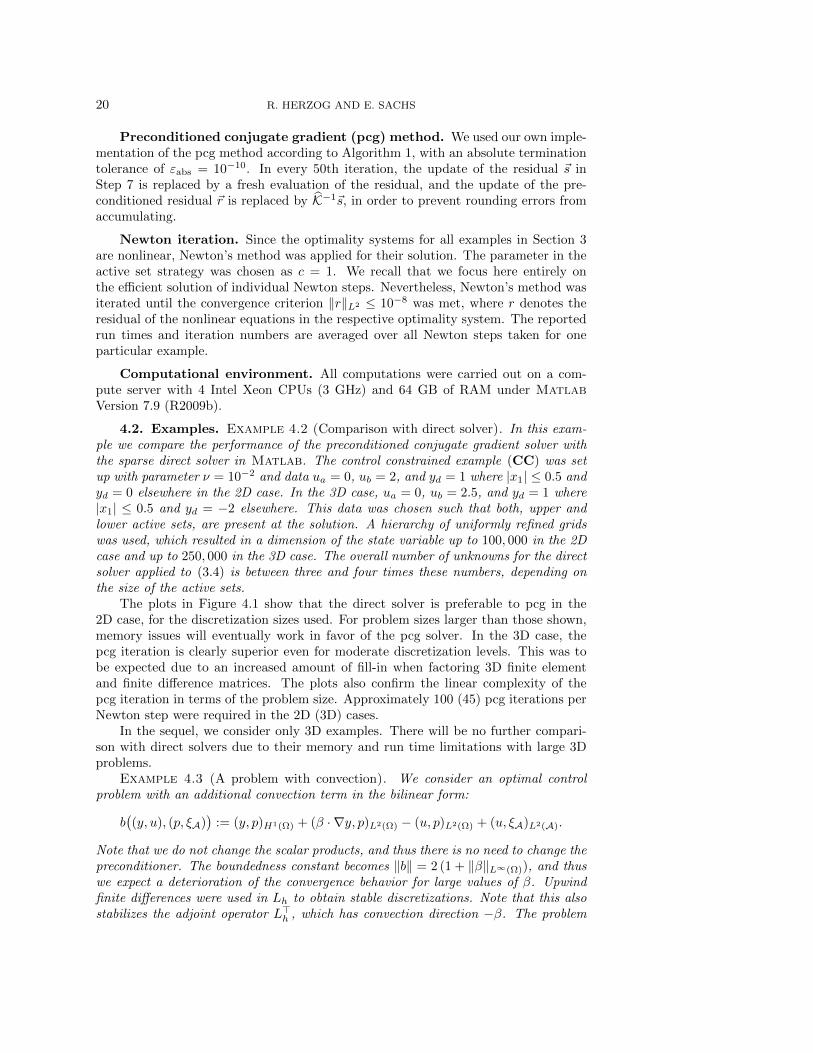
4.2. Examples. Example 4.2 (Comparison with direct solver). In this exam-ple we compare the performance of the preconditioned conjugate gradient solver withthe sparse direct solver in Matlab. The control constrained example (CC) was setup with parameter ν = 10−2 and data ua = 0, ub = 2, and yd = 1 where |x1| ≤ 0.5 andyd = 0 elsewhere in the 2D case. In the 3D case, ua = 0, ub = 2.5, and yd = 1 where|x1| ≤ 0.5 and yd = −2 elsewhere. This data was chosen such that both, upper andlower active sets, are present at the solution. A hierarchy of uniformly refined gridswas used, which resulted in a dimension of the state variable up to 100, 000 in the 2Dcase and up to 250, 000 in the 3D case. The overall number of unknowns for the directsolver applied to (3.4) is between three and four times these numbers, depending onthe size of the active sets.

The plots in Figure 4.1 show that the direct solver is preferable to pcg in the2D case, for the discretization sizes used. For problem sizes larger than those shown,memory issues will eventually work in favor of the pcg solver. In the 3D case, thepcg iteration is clearly superior even for moderate discretization levels. This was tobe expected due to an increased amount of fill-in when factoring 3D finite elementand finite difference matrices. The plots also confirm the linear complexity of thepcg iteration in terms of the problem size. Approximately 100 (45) pcg iterations perNewton step were required in the 2D (3D) cases.

In the sequel, we consider only 3D examples. There will be no further compari-son with direct solvers due to their memory and run time limitations with large 3Dproblems.

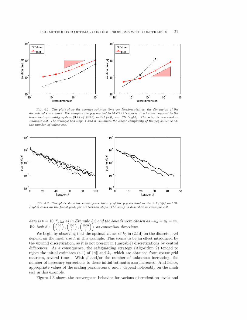
Example 4.3 (A problem with convection). We consider an optimal controlproblem with an additional convection term in the bilinear form:

b((y, u), (p, ξA)

):= (y, p)H1(Ω) + (β · ∇y, p)L2(Ω) − (u, p)L2(Ω) + (u, ξA)L2(A).

Note that we do not change the scalar products, and thus there is no need to change thepreconditioner. The boundedness constant becomes ‖b‖ = 2 (1 + ‖β‖L∞(Ω)), and thuswe expect a deterioration of the convergence behavior for large values of β. Upwindfinite differences were used in Lh to obtain stable discretizations. Note that this alsostabilizes the adjoint operator L>h , which has convection direction −β. The problem


Fig. 4.1. The plots show the average solution time per Newton step vs. the dimension of thediscretized state space. We compare the pcg method to Matlab’s sparse direct solver applied to thelinearized optimality system (3.4) of (CC) in 2D (left) and 3D (right). The setup is described inExample 4.2. The triangle has slope 1 and it visualizes the linear complexity of the pcg solver w.r.t.the number of unknowns.

Fig. 4.2. The plots show the convergence history of the pcg residual in the 2D (left) and 3D(right) cases on the finest grid, for all Newton steps. The setup is described in Example 4.2.

data is ν = 10−2, yd as in Example 4.2 and the bounds were chosen as −ua = ub =∞.

We took β ∈(

1000

),(

10000

),(

100000

)as convection directions.

We begin by observing that the optimal values of k0 in (2.1d) on the discrete leveldepend on the mesh size h in this example. This seems to be an effect introduced bythe upwind discretization, as it is not present in (unstable) discretizations by centraldifferences. As a consequence, the safeguarding strategy (Algorithm 2) tended toreject the initial estimates (4.1) of ‖a‖ and k0, which are obtained from coarse gridmatrices, several times. With β and/or the number of unknowns increasing, thenumber of necessary corrections to these initial estimates also increased. And hence,appropriate values of the scaling parameters σ and τ depend noticeably on the meshsize in this example.

Figure 4.3 shows the convergence behavior for various discretization levels and


values of β. For large values of β, we see a pronounced mesh dependence of theconvergence history. As mentioned above, this is due to the upwind stabilization,which leads to a mesh dependent k0 and thus to a deterioration of the preconditionedcondition number on refined grids.

Fig. 4.3. The left plot shows the solution time for the single Newton step vs. the dimensionof the discretized state space in a series of unconstrained problems with convection. The setup isdescribed in Example 4.3. The right plot displays the convergence history of the pcg residual onvarious grid levels for β = (1000, 0, 0)>.

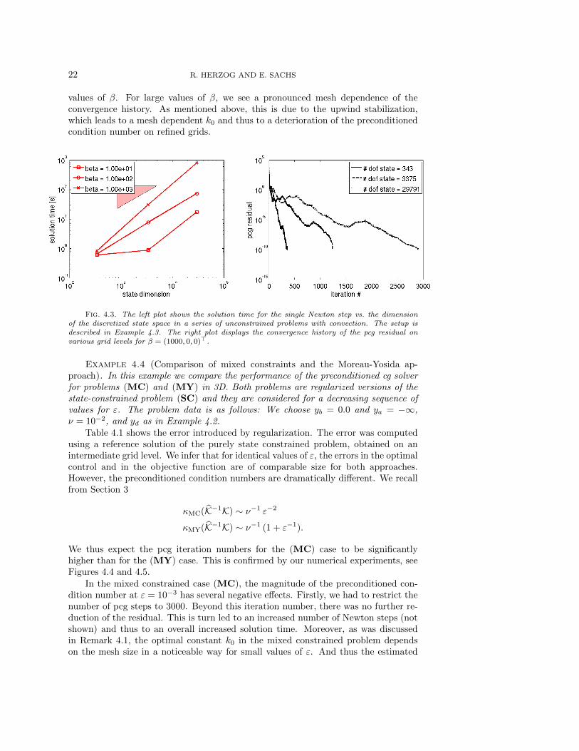
Example 4.4 (Comparison of mixed constraints and the Moreau-Yosida ap-proach). In this example we compare the performance of the preconditioned cg solverfor problems (MC) and (MY) in 3D. Both problems are regularized versions of thestate-constrained problem (SC) and they are considered for a decreasing sequence ofvalues for ε. The problem data is as follows: We choose yb = 0.0 and ya = −∞,ν = 10−2, and yd as in Example 4.2.

Table 4.1 shows the error introduced by regularization. The error was computedusing a reference solution of the purely state constrained problem, obtained on anintermediate grid level. We infer that for identical values of ε, the errors in the optimalcontrol and in the objective function are of comparable size for both approaches.However, the preconditioned condition numbers are dramatically different. We recallfrom Section 3

κMC(K−1K) ∼ ν−1 ε−2

κMY(K−1K) ∼ ν−1 (1 + ε−1).

We thus expect the pcg iteration numbers for the (MC) case to be significantlyhigher than for the (MY) case. This is confirmed by our numerical experiments, seeFigures 4.4 and 4.5.

In the mixed constrained case (MC), the magnitude of the preconditioned con-dition number at ε = 10−3 has several negative effects. Firstly, we had to restrict thenumber of pcg steps to 3000. Beyond this iteration number, there was no further re-duction of the residual. This is turn led to an increased number of Newton steps (notshown) and thus to an overall increased solution time. Moreover, as was discussedin Remark 4.1, the optimal constant k0 in the mixed constrained problem dependson the mesh size in a noticeable way for small values of ε. And thus the estimated


scaling parameters σ and τ had to be corrected several times before the pcg iterationwent through. This led to the superlinear behavior of the run time w.r.t. the numberof state variables in Figure 4.3.

The situation was significantly better in the Moreau-Yosida case (MY). It wascomputationally feasible to reduce ε to 10−5 for this setup. Moreover, the estimatedconstants ‖a‖′ and k′0 on a coarse level were viable for the fine levels as well.

ε ‖uMC− u‖L2 ‖uMY− u‖L2 |JMC− J | |JMY− J |1.00e-01 1.91e+00 1.02e+00 7.04e-02 2.62e-02

1.00e-02 5.25e-01 3.65e-01 9.32e-03 8.56e-03

1.00e-03 9.23e-02 8.05e-02 1.01e-03 1.34e-03

1.00e-04 1.18e-02 1.46e-04

1.00e-05 1.29e-03 1.48e-05

Table 4.1Comparison of errors introduced by the (MC) and (MY) regularizations of the state con-

strained problem (SC). See Example 4.4. JMC and JMY denote the values of the objective func-tionals in problems (MC) and (MY), and J denotes the value of the objective for the unregularizedproblem (SC) solved with a direct solver.

Fig. 4.4. The plot shows the average solution time per Newton step vs. the dimension of thediscretized state space. Both regularization approaches (MC) and (MY) are compared for variouslevels of the regularization parameter ε. The setup is described in Example 4.4.

In Example 4.4, the largest problem solved for ε = 10−5 has about 30,000 statevariables (and the same number of control and adjoint state variables). The solution


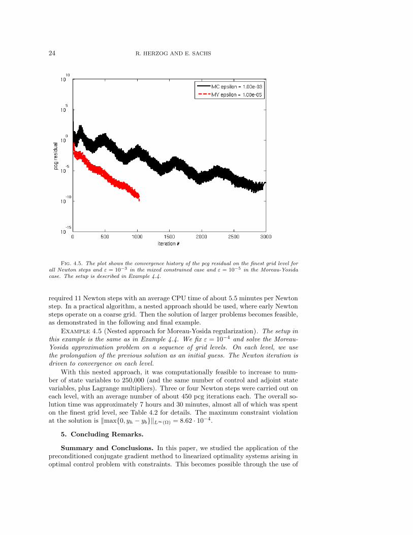
Fig. 4.5. The plot shows the convergence history of the pcg residual on the finest grid level forall Newton steps and ε = 10−3 in the mixed constrained case and ε = 10−5 in the Moreau-Yosidacase. The setup is described in Example 4.4.

required 11 Newton steps with an average CPU time of about 5.5 minutes per Newtonstep. In a practical algorithm, a nested approach should be used, where early Newtonsteps operate on a coarse grid. Then the solution of larger problems becomes feasible,as demonstrated in the following and final example.

Example 4.5 (Nested approach for Moreau-Yosida regularization). The setup inthis example is the same as in Example 4.4. We fix ε = 10−4 and solve the Moreau-Yosida approximation problem on a sequence of grid levels. On each level, we usethe prolongation of the previous solution as an initial guess. The Newton iteration isdriven to convergence on each level.

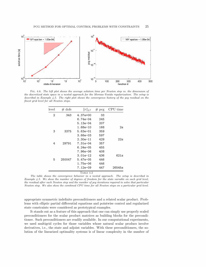
With this nested approach, it was computationally feasible to increase to num-ber of state variables to 250,000 (and the same number of control and adjoint statevariables, plus Lagrange multipliers). Three or four Newton steps were carried out oneach level, with an average number of about 450 pcg iterations each. The overall so-lution time was approximately 7 hours and 30 minutes, almost all of which was spenton the finest grid level, see Table 4.2 for details. The maximum constraint violationat the solution is ‖max0, yh − yb‖L∞(Ω) = 8.62 · 10−4.

5. Concluding Remarks.

Summary and Conclusions. In this paper, we studied the application of thepreconditioned conjugate gradient method to linearized optimality systems arising inoptimal control problem with constraints. This becomes possible through the use of


Fig. 4.6. The left plot shows the average solution time per Newton step vs. the dimension ofthe discretized state space in a nested approach for the Moreau-Yosida regularization. The setup isdescribed in Example 4.5. The right plot shows the convergence history of the pcg residual on thefinest grid level for all Newton steps.

level # dofs ‖r‖L2 # pcg CPU time

2 343 4.37e+00 33

6.74e-04 245

5.13e-04 207

1.68e-10 168 2s

3 3375 5.63e-01 359

3.66e-03 597

2.30e-11 429 22s

4 29791 7.31e-04 357

6.24e-05 455

7.96e-06 408

3.01e-12 436 621s

5 250047 5.47e-05 446

1.75e-06 446

7.12e-09 447 26545s

Table 4.2The table shows the convergence behavior in a nested approach. The setup is described in

Example 4.5. We show the number of degrees of freedom for the state variable on each grid level,the residual after each Newton step and the number of pcg iterations required to solve that particularNewton step. We also show the combined CPU time for all Newton steps on a particular grid level.

appropriate symmetric indefinite preconditioners and a related scalar product. Prob-lems with elliptic partial differential equations and pointwise control and regularizedstate constraints were considered as prototypical examples.

It stands out as a feature of this approach that one can simply use properly scaledpreconditioners for the scalar product matrices as building blocks for the precondi-tioner. Such preconditioners are readily available. In our computational experiments,we used multigrid cycles for those variables whose natural scalar producs involvederivatives, i.e., the state and adjoint variables. With these preconditioners, the so-lution of the linearized optimality systems is of linear complexity in the number of


unknowns, and no partial differential equations need to be solved in the process.

In order to regularize the state constrained problems, mixed control-state con-straints and a Moreau-Yosida penalty approach were considered and compared. Itturned out that from our computational point of view, the penalty approach is clearlysuperior to the mixed constraint approach. At the same level of regularization error,the preconditioned condition numbers are of order 1/ε for the penalty approach butof order 1/ε2 with mixed constraints. This was confirmed by numerical experiments.

The solution of state constrained optimal control problems in 3D is computation-ally challenging. In fact, numerical results are hardly found in the literature. Theapproach presented here pushes the frontier towards larger problems. In our compu-tational experiments, the largest problem solved has about 250,000 state variables,and the same number of control and adjoint state variables, plus Lagrange multipliers.

Outlook. The main effort in every iteration of the pcg loop (Algorithm 1) isthe application of the preconditioner. In our examples, this essentially amounts tothree multigrid cycles and the solution of PAM

−1h P>A ~µA = ~bA (see Algorithm 3).

Thus every pcg iteration is relatively inexpensive. Profiling experiments on the gridwith 250,000 unknowns show that every call to the preconditioner in our Matlabimplementation took about 1.4 seconds. Clearly, there is room for improvement inusing another computational environment and parallel preconditioners, e.g., based ondomain decomposition.

The key issue, however, is to reduce the preconditioned condition number and thusthe number of required pcg iterations. In [19], the authors used scalar products whichdepend on the control cost parameter ν. In this way, they found very low conditionnumbers independent of ν for an unconstrained optimal control problem. They donot discuss, however, the impact of these norms on accuracy and error tolerances.The investigation of ε dependent norms for regularized state constrained problemsin order to reduce the iteration numbers would be worthwhile and is postponed tofollow-up work.

The analysis in [19] relies on the positive semidefiniteness of the (1,1) block A, see(1.3e). In nonlinear optimal control problems, this condition may not be satisfied, noteven in the vicinity of an optimal solution satisfying second-order sufficient conditions.Quasi-Newton techniques could be applied to overcome this problem, but this issuedeserves further investigation.

Finally, we found that upwind stabilization of convection dominated problems canrender the inf–sup constant k0 mesh dependent, which results in a mesh dependentconvergence behavior. Other stabilization techniques without this deficiency shouldthus be prefered.

REFERENCES

[1] A. Battermann and M. Heinkenschloss. Preconditioners for Karush-Kuhn-Tucker MatricesArising in the Optimal Control of Distributed Systems. In W. Desch, F. Kappel, andK. Kunisch, editors, Optimal Control of Partial Differential Equations, volume 126 ofInternational Series of Numerical Mathematics, pages 15–32. Birkhauser, 1998.

[2] A. Battermann and E. Sachs. Block preconditioners for KKT systems in PDE-governed optimalcontrol problems. In Fast solution of discretized optimization problems (Berlin, 2000),volume 138 of Internat. Ser. Numer. Math., pages 1–18. Birkhauser, Basel, 2001.

[3] G. Biros and O. Ghattas. Parallel Lagrange-Newton-Krylov-Schur methods for PDE-constrained optimization. Part I: The Krylov-Schur solver. SIAM Journal on ScientificComputing, 27(2):687–713, 2005.

[4] J. Bramble and J. Pasciak. A preconditioning technique for indefinite systems resulting from


mixed approximations of elliptic problems. Mathematics of Computation, 50(181):1–17,1988.

[5] E. Casas. Control of an elliptic problem with pointwise state constraints. SIAM Journal onControl and Optimization, 24(6):1309–1318, 1986.

[6] S. Dollar, N. Gould, M. Stoll, and A. Wathen. Preconditioning saddle-point systems withapplications in optimization. SIAM Journal on Scientific Computing, 32(1):249–270, 2010.

[7] S. Dollar, N. Gould, and A. Wathen. On implicit-factorization constraint preconditioners.In G. Di Pillo and M. Roma, editors, Large-Scale Nonlinear Optimization, volume 83 ofNonconvex Optimization and its Applications, pages 61–82, Berlin, 2006. Springer.

[8] S. Dollar, N. Gould, and A. Wathen. Implicit-factorization preconditioning and iterative solversfor regularized saddle-point systems. SIAM Journal on Matrix Analysis and Applications,28(1):170–189, 2007.

[9] N. Gould, M. Hribar, and J. Nocedal. On the solution of equality constrained quadratic prob-lems arising in optimization. SIAM Journal on Scientific Computing, 23(4):1375–1394,2001.

[10] R. Griesse. Lipschitz stability of solutions to some state-constrained elliptic optimal controlproblems. Journal of Analysis and its Applications, 25:435–455, 2006.

[11] M. Hintermuller, K. Ito, and K. Kunisch. The primal-dual active set strategy as a semismoothNewton method. SIAM Journal on Optimization, 13(3):865–888, 2002.

[12] M. Hintermuller, I. Kopacka, and S. Volkwein. Mesh-independence and preconditioning for solv-ing control problems with mixed control-state constraints. ESAIM: Control, Optimisationand Calculus of Variations, 15(3), 2009.

[13] K. Ito and K. Kunisch. Semi-smooth Newton methods for state-constrained optimal controlproblems. Systems and Control Letters, 50:221–228, 2003.

[14] K. Ito, K. Kunisch, I. Gherman, and V. Schulz. Approximate nullspace iterations for KKTsystems in model based optimization. SIAM Journal on Matrix Analysis and Applications,31(4):1835–1847, 2010.

[15] T. Mathew, M. Sarkis, and C. Schaerer. Analysis of block matrix preconditioners for ellipticoptimal control problems. Numerical Linear Algebra with Applications, 14:257–279, 2007.

[16] C. Meyer, U. Prufert, and F. Troltzsch. On two numerical methods for state-constrained ellipticcontrol problems. Optimization Methods and Software, 22(6):871–899, 2007.

[17] T. Rees, S. Dollar, and A. Wathen. Optimal solvers for PDE-constrained optimization. SIAMJournal on Scientific Computing, 32(1):271–298, 2010.

[18] T. Rees and M. Stoll. Block triangular preconditioners for PDE constrained optimization.Numerical Linear Algebra with Applications, to appear.

[19] J. Schoberl and W. Zulehner. Symmetric indefinite preconditioners for saddle point problemswith applications to PDE-constrained optimization. SIAM Journal of Matrix Analysis andApplications, 29(3):752–773, 2007.

[20] G. Stadler. Elliptic optimal control problems with L1-control cost and applications for theplacement of control devices. Computational Optimization and Applications, 44(2):159–181, 2009.

[21] F. Troltzsch. Optimale Steuerung partieller Differentialgleichungen. Vieweg, Wiesbaden, 2005.

PRECONDITIONED CONJUGATE GRADIENT METHOD … · PRECONDITIONED CONJUGATE GRADIENT METHOD FOR...

Documents

Transcript of PRECONDITIONED CONJUGATE GRADIENT METHOD … · PRECONDITIONED CONJUGATE GRADIENT METHOD FOR...