JPEG Decoder implementation on FPGA using Dynamic Partial ...

FACHHOCHSCHULESTUTTGART
HO CH SCHULE FÜ RTECHN IK
UNIVERSITY O F A PPLIED SC IENCES
Department of Mathematics and
Computer Science
Winter Term 2001/2002
Implementation of a JPEG Decoder for a 16-bitMicrocontroller
by
Stefan Kuhr
A Thesis Submitted
in Partial Fulfillment of the
Requirements for the Degree
MASTER OF SCIENCE
in
Software Technology
Thesis Committee:
Prof. Dr. Uwe Mußigmann, ChairProf. Dr. Peter HauberRolf Kofink, Sony Corp.


For the bestof all mothers.


Contents
Contents I
Acknowledgements IV
Notational Conventions V
List of Acronyms VI
List of Figures X
List of Tables XII
1 Introduction 11.1 Subject and conceptual formulation of this thesis . . . . . . . . . . . . . . . 11.2 Overview of the subsequent chapters . . . . . . . . . . . . . . . . . . . . . . 3
2 A brief introduction to JPEG encoding and decoding 42.1 History and Motivation . . . . . . . . . . . . . . . . . . . . . . . . . . . . . 42.2 The JPEG Standard . . . . . . . . . . . . . . . . . . . . . . . . . . . . . . . 5
2.2.1 Compression classes . . . . . . . . . . . . . . . . . . . . . . . . . . . 62.2.2 DCT-based Encoding . . . . . . . . . . . . . . . . . . . . . . . . . . 62.2.3 Modes of operation . . . . . . . . . . . . . . . . . . . . . . . . . . . . 92.2.4 The baseline process . . . . . . . . . . . . . . . . . . . . . . . . . . . 10
2.3 The JPEG File Interchange Format (JFIF) . . . . . . . . . . . . . . . . . . 102.4 Compression and information loss in JPEG encoding . . . . . . . . . . . . . 12
3 The Discrete Cosine Transform 173.1 Mathematical Definition of the DCT . . . . . . . . . . . . . . . . . . . . . . 17
3.1.1 The one-dimensional DCT . . . . . . . . . . . . . . . . . . . . . . . . 173.1.2 The two-dimensional DCT . . . . . . . . . . . . . . . . . . . . . . . . 19
3.2 Relations between the DCT and the DFT . . . . . . . . . . . . . . . . . . . 203.2.1 Computing an N-point DCT from a 2N-point DFT . . . . . . . . . . 213.2.2 A Divide-and-Conquer Scheme for real input vectors . . . . . . . . . 213.2.3 DCT and DFT for real and symmetrical input vectors . . . . . . . . 24
3.3 Fast one-dimensional 8-point DCTs . . . . . . . . . . . . . . . . . . . . . . 253.3.1 A simple and fast 8-point DCT . . . . . . . . . . . . . . . . . . . . 263.3.2 The Ligtenberg-Vetterli-DCT . . . . . . . . . . . . . . . . . . . . . 28
I

CONTENTS
3.3.2.1 An algebraic approach to the Ligtenberg-Vetterli-DCT . . 283.3.2.2 A graphical approach to the Ligtenberg-Vetterli-DCT . . . 32
3.3.3 The Loeffler-Ligtenberg-Moschytz-DCT . . . . . . . . . . . . . . . . 383.3.4 The Inverse Loeffler-Ligtenberg-Moschytz-DCT . . . . . . . . . . . 403.3.5 The Winograd 16-point “small-N” DFT . . . . . . . . . . . . . . . . 423.3.6 The Arai-Agui-Nakajima-DCT . . . . . . . . . . . . . . . . . . . . . 493.3.7 The Inverse Arai-Agui-Nakajima-DCT . . . . . . . . . . . . . . . . 61
3.4 Fast two-dimensional DCTs . . . . . . . . . . . . . . . . . . . . . . . . . . . 633.4.1 The tensor product and its properties . . . . . . . . . . . . . . . . . 633.4.2 The two-dimensional DCT as a tensor product . . . . . . . . . . . . 643.4.3 Feig’s fast two-dimensional DCT . . . . . . . . . . . . . . . . . . . . 663.4.4 Feig’s fast two-dimensional inverse DCT . . . . . . . . . . . . . . . . 80
4 Fast Image Scaling in the Context of JPEG Decoding 934.1 Image Scaling in the Spatial Domain . . . . . . . . . . . . . . . . . . . . . . 934.2 Image Scaling in the IDCT Process . . . . . . . . . . . . . . . . . . . . . . . 97
4.2.1 Image scaling in the IDCT process to half of the original size . . . . 974.2.2 Image scaling in the IDCT process to a fourth of the original size . . 994.2.3 Image scaling in the IDCT process to an eighth of the original size . 99
5 The JPEGLib 1015.1 Goals, Motivation and History . . . . . . . . . . . . . . . . . . . . . . . . . 1025.2 Capabilities of the JPEGLib . . . . . . . . . . . . . . . . . . . . . . . . . . . 1035.3 The JPEGLib package content . . . . . . . . . . . . . . . . . . . . . . . . . 1045.4 Adapting the JPEGLib to different platforms and compilers . . . . . . . . . 105
5.4.1 Determining the correct jconfig.h file and the correct makefile . . . . 1055.4.2 Choosing the right memory manager . . . . . . . . . . . . . . . . . . 106
5.5 Usage and Architectural Issues . . . . . . . . . . . . . . . . . . . . . . . . . 1075.5.1 Typical code sequences for encoding . . . . . . . . . . . . . . . . . . 1085.5.2 Typical code sequences for decoding . . . . . . . . . . . . . . . . . . 1095.5.3 The encoder and decoder objects . . . . . . . . . . . . . . . . . . . . 110
5.6 Summary . . . . . . . . . . . . . . . . . . . . . . . . . . . . . . . . . . . . . 111
6 JPEG Decoding on the Micronas SDA 6000 Controller 1146.1 Project descriptions . . . . . . . . . . . . . . . . . . . . . . . . . . . . . . . 1146.2 Changes to the JPEGLib . . . . . . . . . . . . . . . . . . . . . . . . . . . . 1156.3 Changes for faster downscaling to a fourth . . . . . . . . . . . . . . . . . . . 1216.4 Important compiler optimization settings . . . . . . . . . . . . . . . . . . . 1276.5 The custom data source manager for M2 . . . . . . . . . . . . . . . . . . . . 1276.6 Other implementations of custom functionality . . . . . . . . . . . . . . . . 128
6.6.1 “Hooking” into Huffman decoding . . . . . . . . . . . . . . . . . . . 1296.6.2 Using XRAM for the range-limit table . . . . . . . . . . . . . . . . . 1306.6.3 Modifying the color conversion and upsampling subobjects . . . . . 1306.6.4 Modifying the dithering subobjects . . . . . . . . . . . . . . . . . . . 131
6.7 Customizing the behaviour of the Software . . . . . . . . . . . . . . . . . . 1326.8 Results . . . . . . . . . . . . . . . . . . . . . . . . . . . . . . . . . . . . . . . 133
6.8.1 Memory limitations and high-resolution JPEG files . . . . . . . . . . 133
II

CONTENTS
6.8.2 4-4-4 mode versus 5-6-5 mode . . . . . . . . . . . . . . . . . . . . . . 1346.8.3 JPEG Performance . . . . . . . . . . . . . . . . . . . . . . . . . . . . 1346.8.4 Image scaling Performance . . . . . . . . . . . . . . . . . . . . . . . 1386.8.5 Debugging versus “Free-Run” Performance . . . . . . . . . . . . . . 138
7 Summary and Future Outlook 140
Index 143
Bibliography 145
Declaration 148
III

Acknowledgements
The author would like to thank Sony-Wega Corporation for the opportunity to work on thisinteresting topic as a master thesis. Special thanks go to all the fine folks of the VEE team ofthe Sony Advanced Technology Center Stuttgart, especially to the author’s supervisor, RolfKofink, for all the fruitful discussions, to Andreas Beermann and Thor Opl for insightfulcomments, to Matthias Jerye for his outstanding technical expertise and cooperativeness,and to Mark Blaxall for reviewing this document over and over again, providing useful tipsfrom a native English speaker.
Special thanks go to Thomas G. Lane from the Independent JPEG Group for reviewingchapter 5.
Finally, the author would like to thank all the helpful people in the German speakingTEX usenet newsgroup de.comp.text.tex for helping troubleshoot all kinds of weirdnessesinvolved with writing a document like this in LATEX.
IV

Notational Conventions
The following notational conventions will be used throughout this document:
Symbol Meaning
F (u) One-dimensional Fourier TransformF (u, v) Two-dimensional Fourier TransformF (u) One-dimensional Cosine TransformF (u, v) Two-dimensional Cosine Transform<{. . .} Real Part={. . .} Imaginary Partj
√−1
In n× n Identity Matrix
V

List of Acronyms
2D-DCT Two-dimensional Discrete Cosine Transform. The 2D-DCT is the two-dimensio-nal variant of the DCT, see section 3.1.2.
2D-FDCT Two-dimensional Forward Discrete Cosine Transform. The 2D-FDCT is thetwo-dimensional variant of the FDCT, see section 3.1.2.
2D-IDCT Two-dimensional Inverse Discrete Cosine Transform. The 2D-IDCT is the two-dimensional variant of the IDCT, see section 3.1.2.
AC Alternating Current. In electricity, Alternating Current occurs when charge carriersin a conductor or semiconductor periodically reverse their direction of movement.
AC-3 Audio Code number 3. AC-3 is a multichannel music compression technology, alsoknown as Dolby Digital, that has been developed by Dolby Laboratories.
ANSI American National Standards Institute. The American National Standards Instituteis the primary organization for fostering the development of technology standards inthe United States of America. ANSI works with industry groups and is the UnitedStates’ member of the ISO and the IEC.
ASCII American Standard Code for Information Interchange. ASCII is the most commonformat for text files in computers and on the Internet. It was developed by the ANSI.
CCITT International Telegraph and Telephone Consultative Committee. The CCITT isan organ of the ITU.
CMYK Cyan, Magenta, Yellow, Black. CMYK is a so-called color space and thus refersto a system for representing colors. The CMYK color space is mainly used for printedcolor illustrations.
COM Component Object Model. COM is a framework and an architecture for creation,distribution and managing of distributed objects in a network, as specified by Mi-crosoft.
cos-DFT Cosine DFT. The Cosine DFT is the definition of Vetterli and Nussbaumer forthe real part of a DFT, see section 3.2.2.
CORBA Common Object Request Broker Architecture. CORBA is an architecture andspecification for creation, distribution and managing of distributed objects in a net-work, as defined by the OMG (Object Management Group).
VI

LIST OF ACRONYMS
DC Direct Current. DC (Direct Current) is the unidirectional flow or movement of electriccharge carriers.
DCT Discrete Cosine Transform. The Discrete Cosine Transform is an orthonormal trans-form that is suitable for image compression, see chapter 3.
DCT* Scaled variant of the FDCT. The DCT* is a scaled variant of the FDCT, see section3.2.2.
DFT Discrete Fourier Transform. The Discrete Fourier Transform is an orthonormal trans-form that is widely used in system theory, see section 3.2.1.
DRAM Dynamic Random Access memory. Dynamic Random Access memory is the mostcommon kind of random access memory (RAM) for personal computers.
EPROM Erasable programmable read-only memory. EPROM is programmable read-onlymemory that can be erased by exposing it to ultraviolet light in order to reprogramit.
FDCT Forward Discrete Cosine Transform. See the complete definition of the ForwardDiscrete Cosine Transform in 3.1.1.
GDI Graphics Device Interface. The GDI is a software library that was used throughoutthis thesis in conjunction with the microcontroller in use for the rendering of bitmapson a monitor or TV set.
GIF Graphics Interchange Format. GIF is one of the most common file formats for graphicimages on the World Wide Web.
GNU GNU is not Unix. The recursive acronym GNU stands for a UNIX-like operatingsystem that comes with source code that can be copied, modified, and redistributed.Often the term GNU is also associated with “The GNU project” of the Free SoftwareFoundation.
HDTV High Definition Television. HDTV is is a television format in 16:9 aspect ratiowith at least twice the horizontal and vertical resolution of the standard format.
IDCT Inverse Discrete Cosine Transform. The Inverse Discrete Cosine Transform is thereverse process to the FDCT. See the complete definition of the Inverse Discrete CosineTransform in 3.1.1.
IEC International Electrotechnical Commission. The IEC is a nongovernmental standardsassociation that coordinates and unifies electrotechnical standards.
IJG Independent JPEG Group. An informal group that writes and distributes a widelyused free library for JPEG image compression.
IRAM Internal dual-port RAM. The IRAM is on-chip memory of the controller usedthroughout this thesis.
ISO International Organization for Standardization. The ISO is a worldwide federation ofnational standards bodies.“ISO” is actually not an abbreviation. It is a word, derivedfrom the Greek isos, meaning “equal”.
VII
LIST OF ACRONYMS
ITU International Telecommunication Union. The ITU is the United Nations’ SpecializedAgency in the field of telecommunications.
JFIF JPEG File Interchange Format. JFIF is the standard file format for exchangingJPEG images, see section 2.3.
JPEG Joint Photographic Expert Group. JPEG is the standard for continuous tone stillimages, see chapter 2.
MIPS Million instructions per second. The number of MIPS corresponds to the numberof operations a computer can execute within a given time and thus serves as a generalmeasure of computing performance.
MMX Multimedia Extensions. MMX is an extension to the instruction set of the IntelPentium processor family for improved performance of multimedia applications.
MPEG Moving Picture Experts Group. The Moving Picture Experts Group is a workinggroup in ISO that develops standards for digital video and audio compression.
OS Operating System. An Operating System is the program that is being initially loadedinto a computer by a boot procedure and that manages all the other programs in thecomputer.
PAL Phase Alternation Line. PAL is an analog television display standard that is mainlyused in Europe but also in other parts of the world.
ROM Read-only Memory. Read-only Memory is memory that cannot be written to.
RGB Red, Green, Blue. RGB is a so-called color space and thus refers to a system for rep-resenting colors. Pixels are represented as tupels of red, green and blue components.
sin-DFT Sine DFT. The Sine DFT is the definition of Vetterli and Nussbaumer for theimaginary part of a DFT, see section 3.2.2.
SVGA Super Video Graphics Array. SVGA is a display mode for computer monitors asspecified by the Video Electronics Standards Assocation (VESA).
SMP Symmetrical Multiprocessing. In systems that employ Symmetrical Multiprocessing,more than one processor is used and a single copy of the operating system is in chargeof all the processors. The operating system does not monopolize a single CPU, i.e.both operating system code and application code can run on all available processors.
UNICODE The Unicode Worldwide Character Standard. UNICODE is a format for bi-nary coding text files in computers. UNICODE encompasses all the diverse languagesof the modern world as well as many classical and historical languages.
UI User Interface. The User Interface is the part of a computer program that accepts inputfrom the user and produces output for the user.
Win32 32-bit Windows. 32-bit Windows is the operating system environment that theMicrosoft Windows operating systems provide to applications.
VIII

LIST OF ACRONYMS
XRAM Internal XBUS RAM. The XRAM is on-chip memory of the controller usedthroughout this thesis.
YCCK Luminance, Chroma, Chroma, Black. YCCK is a so-called color space and thusrefers to a system for representing colors. The YCCK color space is a rarely usedcolor space defined by Adobe.
YCbCr Luminance and Chroma. YCbCr is a so-called color space and thus refers to asystem for representing colors. Pixels are represented as tupels of one luminance (Y)and two chroma components (Cb and Cr). For a definition, see section 2.3.
IX

List of Figures
2.1 Simplified diagram of a DCT-based encoder . . . . . . . . . . . . . . . . . . 62.2 Differential encoding of the DC values of two subsequent 8× 8 blocks . . . 72.3 Zig-Zag encoding of AC coefficients within one 8× 8 block . . . . . . . . . . 72.4 Simplified diagram of a DCT-based decoder . . . . . . . . . . . . . . . . . . 82.5 Original picture at size 480000 bytes . . . . . . . . . . . . . . . . . . . . . . 132.6 JPEG file at size 54680 bytes . . . . . . . . . . . . . . . . . . . . . . . . . . 142.7 JPEG file at size 35336 bytes . . . . . . . . . . . . . . . . . . . . . . . . . . 142.8 JPEG file at size 18573 bytes . . . . . . . . . . . . . . . . . . . . . . . . . . 152.9 JPEG file at size 10807 bytes . . . . . . . . . . . . . . . . . . . . . . . . . . 15
3.1 A graphical description of an 8 point real DFT . . . . . . . . . . . . . . . . 333.2 A graphical description of an 8 point DCT* . . . . . . . . . . . . . . . . . 343.3 A combination of figures 3.1 and 3.2 to derive the DCT from the DCT* . . 353.4 Flowgraph for the Ligtenberg-Vetterli Fast DCT . . . . . . . . . . . . . . . 363.5 Hardware implementation of the Ligtenberg-Vetterli Fast DCT . . . . . . . 373.6 Flowgraph for the Loeffler-Ligtenberg-Moschytz Fast DCT . . . . . . . . . . 383.7 Inverse Loeffler-Ligtenberg-Moschytz Fast DCT . . . . . . . . . . . . . . . . 413.8 Flowgraph for the even coefficients of the Arai-Agui-Nakajima Fast DCT . 553.9 Flowgraph for the odd coefficients of the Arai-Agui-Nakajima Fast DCT . . 583.10 Flowgraph for the Arai-Agui-Nakajima Fast DCT . . . . . . . . . . . . . . . 593.11 Flowgraph for the inverse Arai-Agui-Nakajima Fast DCT . . . . . . . . . . 623.12 Flowgraph for matrix AF . . . . . . . . . . . . . . . . . . . . . . . . . . . . 683.13 Flowgraph for matrix MF . . . . . . . . . . . . . . . . . . . . . . . . . . . . 693.14 Flowgraph for matrix BF . . . . . . . . . . . . . . . . . . . . . . . . . . . . 693.15 Flowgraph for matrix AF ⊗AF . . . . . . . . . . . . . . . . . . . . . . . . . 713.16 Flowgraph for matrix BF ⊗BF . . . . . . . . . . . . . . . . . . . . . . . . . 733.17 Flowgraph for matrix M2 . . . . . . . . . . . . . . . . . . . . . . . . . . . . 743.18 Flowgraph for matrix N1 . . . . . . . . . . . . . . . . . . . . . . . . . . . . 753.19 Flowgraph for matrix N2 . . . . . . . . . . . . . . . . . . . . . . . . . . . . 763.20 Flowgraph for matrix N3 = N ⊗ N . . . . . . . . . . . . . . . . . . . . . . . 763.21 Flowgraph for matrix M3 = N ⊗MF . . . . . . . . . . . . . . . . . . . . . . 773.22 Flowgraph of K ′
8 ⊗K ′8 without the final permutation by (P ⊗ P ) . . . . . . 79
3.23 Flowgraph for matrix AI . . . . . . . . . . . . . . . . . . . . . . . . . . . . . 823.24 Flowgraph for matrix BI . . . . . . . . . . . . . . . . . . . . . . . . . . . . . 823.25 Flowgraph for matrix MI . . . . . . . . . . . . . . . . . . . . . . . . . . . . 833.26 Flowgraph for matrix BI ⊗BI . . . . . . . . . . . . . . . . . . . . . . . . . 85
X
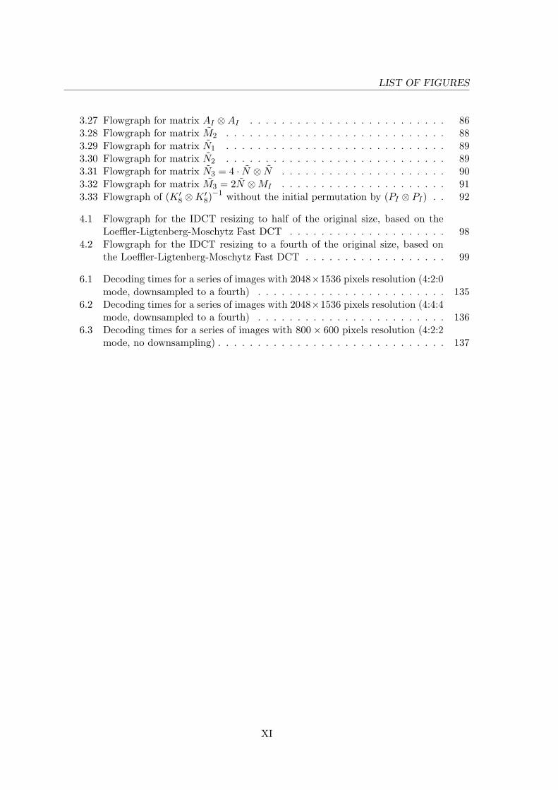
LIST OF FIGURES
3.27 Flowgraph for matrix AI ⊗AI . . . . . . . . . . . . . . . . . . . . . . . . . 863.28 Flowgraph for matrix M2 . . . . . . . . . . . . . . . . . . . . . . . . . . . . 883.29 Flowgraph for matrix N1 . . . . . . . . . . . . . . . . . . . . . . . . . . . . 893.30 Flowgraph for matrix N2 . . . . . . . . . . . . . . . . . . . . . . . . . . . . 893.31 Flowgraph for matrix N3 = 4 · N ⊗ N . . . . . . . . . . . . . . . . . . . . . 903.32 Flowgraph for matrix M3 = 2N ⊗MI . . . . . . . . . . . . . . . . . . . . . 913.33 Flowgraph of (K ′
8 ⊗K ′8)−1 without the initial permutation by (PI ⊗ PI) . . 92
4.1 Flowgraph for the IDCT resizing to half of the original size, based on theLoeffler-Ligtenberg-Moschytz Fast DCT . . . . . . . . . . . . . . . . . . . . 98
4.2 Flowgraph for the IDCT resizing to a fourth of the original size, based onthe Loeffler-Ligtenberg-Moschytz Fast DCT . . . . . . . . . . . . . . . . . . 99
6.1 Decoding times for a series of images with 2048×1536 pixels resolution (4:2:0mode, downsampled to a fourth) . . . . . . . . . . . . . . . . . . . . . . . . 135
6.2 Decoding times for a series of images with 2048×1536 pixels resolution (4:4:4mode, downsampled to a fourth) . . . . . . . . . . . . . . . . . . . . . . . . 136
6.3 Decoding times for a series of images with 800× 600 pixels resolution (4:2:2mode, no downsampling) . . . . . . . . . . . . . . . . . . . . . . . . . . . . . 137
XI

List of Tables
3.1 Computational complexity of Feig’s 2D DCT . . . . . . . . . . . . . . . . . 78
5.1 Revision History of the JPEGLib . . . . . . . . . . . . . . . . . . . . . . . . 1035.2 Memory manager implementations supplied by the JPEGLib . . . . . . . . 106
6.1 Deviations of the new implementation from the standard implementation . 1266.2 Debugging versus “Free Run” Performance . . . . . . . . . . . . . . . . . . 139
XII


Chapter 1
Introduction
All programmers are optimists. Perhaps this modern sorcery especially attractsthose who believe in happy endings and fairy godmothers. Perhaps the hundredof nitty frustrations drive away all but those who habitually focus on the endgoal. Perhaps it is merely that computers are young, programmers are younger,and the young are always optimists.
– From the book “The mythical man-month”by Frederick P. Brooks jr., 1975
The aim of this chapter is to provide the reader with the initial expectations prior tothe beginning of this thesis, as well as with information regarding the organization of
the rest of this document. For the hasty reader it is probably enough to read the followingsection, section 1.1, and the summary in chapter 7, to get an impression of what this thesisis all about. For all other readers, section 1.2 contains an overview of what the reader willexpect throughout the rest of this document.
1.1 Subject and conceptual formulation of this thesis
This thesis is considered a feasibility study, that should examine whether a typical 16-bitmicrocontroller with a graphics accelerator unit (Micronas SDA 6000), as it is used for On-Screen-Displays in High-End TV sets, is capable of decoding JPEG files of commonly usedfile sizes and image resolutions. Of particular interest are those resolutions that are com-mon for digital still cameras. In order to estimate the feasibility, which first of all includesacceptable performance, a JPEG decoder has to be implemented on the microcontroller.
The following issues have been identified beforehand as potential obstacles for this goal:
• Limited memory resources of the controller: The controller can use a maximum of 8MBytes of DRAM. While this seems to be enough for JPEG decoding at first glance,it has to be considered that an embedded device such as a microcontroller doesn’t havevirtual memory like PCs or workstations due to the lack of a harddisk. Also, typical
1

CHAPTER 1. INTRODUCTION
JPEG images from digital still cameras at the time of writing are “3.3 Megapixel”images with a resolution of 2048× 1536 pixels. One image of this size with 1 byte percolor component clearly exceeds the available memory space of 8 MBytes.
• Processor speed: The microcontroller runs at a clock rate of 33 MHz. Typical ma-chine instructions need two clock cycles, so the controller can be roughly considereda 16.5 MIPS machine. Typical desktop computers today have several hundred MIPSof processing power and optimized architectures for floating point arithmetics or in-struction sets that are more suitable for the fast calculation of the DCT (DiscreteCosine Transform), like the MMX technology from Intel.
• Display functionality: With standard software packages, the microcontroller’s graphicsaccelerator unit is only capable of rendering RGB tupels with a color depth of 4 bits percolor component on the output device (4-4-4 mode). Though the graphics acceleratorunit has a mode (5-6-5 mode)in which it can display RGB tupels with 5, 6 and 5 bitsfor R, G and B, respectively, there is no software available that exploits this mode.
The following tasks are considered prerequisites for a successful implementation of a JPEGdecoder:
• Availability of suitable software: Part of the work is considered market research forsuitable software packages that could be ported to the microcontroller. The choice ofprogramming languages is limited to C or C++ (via a C++ frontend compiler).
• Familiarity with the development environment for the microcontroller: Masteringthe “tool chain” of C/C++ compiler, assembler, linker/locator and debugger is aprerequisite for writing any software on any platform, but is especially true for thedevelopment for an embedded system with a cross-compiler and a remote debugger,where also the quality of the development tools is generally not as high as for the PCand workstation market.
The following issues are considered additional development goals:
• It should be taken into account, that the TV set used to render a decoded JPEG filetypically has only a very limited spatial resolution. This limitation is imposed by thecapabilities of the microcontroller (800×600 pixels maximum). Therefore, the abilityto scale an image fast enough, either during decoding or after decoding, in order tofit the screen, is a requirement.
• It should be possible to identify and fix possible performance bottlenecks in the soft-ware being used for JPEG decoding. Therefore intimate knowledge of all the stepsinvolved in JPEG decoding, especially the IDCT (Inverse Discrete Cosine Transform),is a requirement.
The minimum result of this thesis should be to make a statement, as to whether or not themicrocontroller is capable of doing JPEG decoding. If it is not, the reasons for this should begiven. If it is capable for doing so, the limitations for this should be determined. Also, theperformance should be determined and increased, and it should be at least possible to decodeimages of standard VGA resolution (640 × 480 pixels). If performance is unacceptable, itshould be possible to predict the processing power that is required for the next generationsof microcontrollers to deliver acceptable performance.
2

1.2. OVERVIEW OF THE SUBSEQUENT CHAPTERS
1.2 Overview of the subsequent chapters
The next chapters are organized as follows: Chapter 2 will contain a brief introduction toJPEG, including some historical retrospect and an overview of those parts of this interna-tional standard that are actually in use at the time of writing. Chapter 3 will dive into theheart of JPEG compression, the discrete cosine transform. Several historical algorithms willbe presented, including the fastest one-dimensional algorithms known up to now, and a fasttwo-dimensional algorithm that is based on the fastest scaled one-dimensional algorithm.Chapter 4 will deal with fast image scaling, either in the spatial domain, after decodinga JPEG image, or during the decoding process. Chapter 5 will give an overview of themost popular software package being used for JPEG encoding and decoding, the Indepen-dent JPEG Group’s JPEGLib. Chapter 6 will include information about the source codewritten during this thesis along with detailed numbers on the performance of the MicronasSDA 6000 microcontroller for JPEG decoding. Chapter 7 will then finally conclude thisdocument with a summary and recommendations for future work.
3

Chapter 2
A brief introduction to JPEGencoding and decoding
Not for nothing does it say in the Commandments “Thou shalt not make untothee any image” . . . Every image is a sin . . .When you love someone you leaveevery possibility open to them, and in spite of all the memories of the past youare ready to be surprised, again and again surprised, at how different they are,how various, not a finished image.
– From the novel “Stiller” by Max Frisch, 1954
The aim of this chapter is to provide an overview of JPEG encoding and decoding withoutgoing too far into the technical details themselves. The interested reader may consult
the various references for more in-depth details on the actual file format or other subtledetails of the standard. First we will give some historical overview and will make clear, thatthe JPEG standard is not, at least in its initial design, a simple file format specification, butrather an architecture for a set of image compression functions with a rich set of capabilities,making it suitable for a wide range of applications that use image compression. We will givean overview of how the encoding and decoding processes actually work and what modesof operation are possible, which ones are actually in use at the time of writing, and whichones are the dominant ones. After that, the definition of the baseline system and the JFIFfile format, which is the prevalent JPEG file format in use today will be given. Finally, wewill conclude this chapter and show, where actually compression and data loss comes intoplay in JPEG encoding.
2.1 History and Motivation
In the early eighties of the 20th century, researchers interested in color image data com-pression initiated some activity in ISO (International Organization for Standardization) ona standard in the area of color image data compression. At about the same time, sev-eral working groups of the CCITT (International Telegraph and Telephone Consultative
4

2.2. THE JPEG STANDARD
Committee), an organ of the ITU (International Telecommunication Union), the UnitedNations’ Specialized Agency in the field of telecommunications, were driven by the samegoal. In order to avoid the definition of two different competing standards, the groups inCCITT joined the working groups in ISO in 1986. In 1987, ISO and the IEC (Interna-tional Electrotechnical Commission) created the Joint Technical Committee 1 (JTC1) inorder to standardize on the field of information technology, and one of these collaborationsunder JTC1 was the now called JPEG committee (pronounce: “Jay-Peg”)1. JPEG standsfor “Joint Photographic Experts Group” and the term “Joint” reflects the fact, that thisstandard was a joint development of the three aforementioned standards bodies.
Finally, in 1992, the JPEG’s standard document ([5]) with the title “Information Tech-nology - Digital Compression and coding of continuous-tone still images - requirements andguidelines” was approved as ISO International Standard 10918-1 (ISO IS 10918-1) and asCCITT Recommendation T.81. To quote from its introduction, this standards document
“. . . sets out requirements and implementation guidelines for continuous-tonestill image encoding and decoding processes, and for the coded representation ofcompressed image data for interchange between applications. These processesand representations are intended to be generic, that is, to be applicable to abroad range of applications for color and grayscale still images within commu-nications and computer systems. [. . . ] In addition to the applications addressedby the CCITT and ISO/IEC, the JPEG committee has developped a compres-sion standard to meet the needs of other applications as well, including desktoppublishing, graphic arts, medical imaging and scientific imaging.” [5].
2.2 The JPEG Standard
The JPEG standards document specifies three elements: an encoder, a decoder and aninterchange format. The encoder takes digital source image data and table specifications asinput, and generates compressed image data via a specified set of procedures. The decodertakes compressed image data and table specifications as input, and generates digitally re-constructed image data via another specified set of procedures. The interchange format isa compressed image data representation that includes all table specifications used in theencoding and decoding process. The interchange format is for exchange between differentapplication environments, e.g. two different computers, computer applications or telecom-munication devices. Both the encoder and the decoder can be implemented in hardwareor software. The interchange format can be data that is transmitted via communicationsfacilities or a file in a computer system. Also, the interchange format does not specify acomplete coded image representation, e.g. application-dependent information such as colorspace is outside the scope of the JPEG specification. This means, that JPEG as such is a“colorblind” specification (see also section 2.3).
In the following sections we will give a rough introduction into some of the JPEGcoding and decoding techniques, based on the standards document ([5]) and the textbook-like approach of [22], whose authors were members of the JPEG working group and wrotesubstantial parts of the standards document during the standardization process. By no
1The reason why three standards bodies bother about standardization on a single area, like in the case ofcolor image data compression, lies in the fact that this area is both part of the telecommunications technologydomain (CCITT) and the computer technology domain (ISO and IEC).
5

CHAPTER 2. A BRIEF INTRODUCTION TO JPEG ENCODING AND DECODING
8 x 8 Pixelblocks
FDCT Quantizer Entropyencoder
Tablespecifications
Tablespecifications
Source Image Data CompressedImage Data
DCT based encoder
Figure 2.1: Simplified diagram of a DCT-based encoder
means should the following be considered a detailed description of the JPEG standard orthe file formats in use today; rather it should give the reader a rough overview of theprocesses involved in JPEG encoding and decoding. For a detailed description of theseissues, the reader may consult [5] and [22].
2.2.1 Compression classes
The JPEG specification specifies two fundamental classes of encoding and decoding pro-cesses: lossy and lossless processes. The processes that are based on the discrete cosinetransform (see chapter 3) are lossy, and thereby allow for substantial compression whileproducing a reconstructed image that shows high visual fidelity to the encoder’s originalsource image. In order to meet the needs of applications requiring lossless compression, theJPEG specification provides the second class of coding processes which is not based on theDCT. For the DCT-based processes, two alternative sample precisions are specified in thestandards document: either 8 bits or 12 bits per sample. 12 bits per sample are only inuse in specialized applications such as medical imaging. For lossless processes the sampleprecision is specified to be from 2 to 16 bits.
In the following, we will disregard the lossless JPEG compression class, because it is notin widespread use2.
2.2.2 DCT-based Encoding
Figure 2.1 shows the encoding process for the case of an image with only one color component(i.e. a grayscale image) in a simplified form. In the case of more than one color component(the number of allowed color components per image in the JPEG specification is virtuallyunlimited) each color component is treated in the same manner, independently of the othercolor components.
In the encoding process the input component’s samples are grouped into 8 × 8 pixelblocks, and each individual block is transformed by the forward DCT (FDCT) into a setof 64 values referred to as the “DCT coefficients” (for an in-depth introduction into theFDCT, see chapter 3). The upper left value of these values is commonly referred to as the
2Ironically, for lossless compression in digital still cameras, TIFF Rev. 6.0 was adopted in [14] instead ofthe lossless JPEG compression class, whereas for lossy compression the JPEG baseline system (see section2.2.4) was adopted.
6

2.2.2. DCT-BASED ENCODING
i i+1BlockBlock
DC i DC i+1
Diff = DC - DC ii+1
Figure 2.2: Differential encoding of the DC values of two subsequent 8× 8 blocks
DC AC 01 AC 07
AC 77AC 70
Figure 2.3: Zig-Zag encoding of AC coefficients within one 8× 8 block
“DC coefficient” or “DC value” (see figure 2.3), because it contains the average value of allpixels prior to the FDCT step. The other 63 values are commonly referred to as the “ACcoefficients” or “AC values”. Each of these 64 coefficients is then divided (“quantized”) byone of 64 corresponding values from a quantization table. There are no default values forquantization tables specified in the JPEG specification3; applications or their users mayspecify values in order to customize image quality for their particular viewing conditions,display devices or preferred image characteristics.
After quantization, the DC coefficient and the 63 AC coefficients are prepared for en-tropy encoding, as shown in figures 2.2 and 2.3: Figure 2.2 exemplifies how the currentquantized DC coefficient is used to predict the subsequent quantized DC coefficient in thatonly the difference between the two is encoded. The underlying heuristics here are, that
3However, the JPEG standard ([5]) gives example tables whose properties are described as follows: “Theseare based on psychovisual thresholding and are derived empirically using luminance and chrominance and2:1 horizontal subsampling. These tables are provided as examples only and are not necessarily suitable forany particular application.”
7

CHAPTER 2. A BRIEF INTRODUCTION TO JPEG ENCODING AND DECODING
IDCTDequantizerEntropydecoder
Tablespecifications
Tablespecifications
ReconstructedImage Data
DCT based decoder
CompressedImage Data
Figure 2.4: Simplified diagram of a DCT-based decoder
the DC values of two subsequent 8 × 8 blocks will not differ too much and that thereforetheir difference can be efficiently encoded with an entropy encoding scheme. The 63 quan-tized AC coefficients do not undergo such a differential encoding technique, but are ratherconverted into a one-dimensional zig-zag sequence, as shown in figure 2.3. After that, thequantized coefficients in zig-zag sequence are passed to an entropy encoding procedure whichcompresses the data further. One of two entropy coding procedures can be used, Huffmancoding or arithmetic coding. For Huffman encoding, the Huffman table specifications mustbe provided to the encoder. For each color component, there must be one Huffman tablefor encoding the DC coeffients and one Huffman table for encoding the AC coefficients,although two color components may share a pair of Huffman tables, as is often the case forthe chroma components (the Cb and Cr components in the YCbCr color space4). In thefollowing we will disregard arithmetic coding, since it is not in widespread use5, although itis generally considered to be slightly more efficient than Huffman coding. Huffman encodingis an entropy encoding procedure that assigns a variable length code to each input symbol.In Huffman encoding, symbols are assigned a frequency that determines their position ina binary tree: Rarely used symbols are at the bottom of the tree whereas frequently usedsymbols are nearer to the tree’s root. A symbol can now be expressed by its Huffmancode, which is the path from the root to its location in the tree. Frequently used symbolsare assigned shorter Huffman codes whereas rarely used symbols are expressed by longerHuffman codes, resulting in overall compression. In JPEG, the Huffman code length (thedepth of the tree) is restricted to 16 bits and the Huffman tables consist of 16 values thatcorrespond to the number of counts of Huffman codes for the associated code length and alist of symbol values that are sorted by Huffman code (see [5]) in order of increasing codelength. From this information, the binary tree can be easily reconstructed, but the JPEGstandard also provides algorithms that can reconstruct the symbols in the input stream ofthe Huffman decoder directly from this information (see [5]).
Figure 2.4 now shows the decoding process in a simplified form. Before the start of the
4In practical usage of JPEG, the preferred color space is not RGB, but rather YCbCr, see also section2.3
5Arithmetic coding is also subject to a patent issue, which caused application developers – or morespecific: the implementors of the Independent JPEG Group’s JPEGLib (see chapter 5) – to refrain fromimplementing arithmetic coding.
8
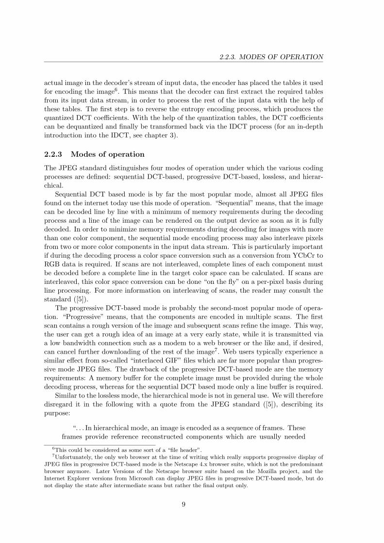
2.2.3. MODES OF OPERATION
actual image in the decoder’s stream of input data, the encoder has placed the tables it usedfor encoding the image6. This means that the decoder can first extract the required tablesfrom its input data stream, in order to process the rest of the input data with the help ofthese tables. The first step is to reverse the entropy encoding process, which produces thequantized DCT coefficients. With the help of the quantization tables, the DCT coefficientscan be dequantized and finally be transformed back via the IDCT process (for an in-depthintroduction into the IDCT, see chapter 3).
2.2.3 Modes of operation
The JPEG standard distinguishes four modes of operation under which the various codingprocesses are defined: sequential DCT-based, progressive DCT-based, lossless, and hierar-chical.
Sequential DCT based mode is by far the most popular mode, almost all JPEG filesfound on the internet today use this mode of operation. “Sequential” means, that the imagecan be decoded line by line with a minimum of memory requirements during the decodingprocess and a line of the image can be rendered on the output device as soon as it is fullydecoded. In order to minimize memory requirements during decoding for images with morethan one color component, the sequential mode encoding process may also interleave pixelsfrom two or more color components in the input data stream. This is particularly importantif during the decoding process a color space conversion such as a conversion from YCbCr toRGB data is required. If scans are not interleaved, complete lines of each component mustbe decoded before a complete line in the target color space can be calculated. If scans areinterleaved, this color space conversion can be done “on the fly” on a per-pixel basis duringline processing. For more information on interleaving of scans, the reader may consult thestandard ([5]).
The progressive DCT-based mode is probably the second-most popular mode of opera-tion. “Progressive” means, that the components are encoded in multiple scans. The firstscan contains a rough version of the image and subsequent scans refine the image. This way,the user can get a rough idea of an image at a very early state, while it is transmitted viaa low bandwidth connection such as a modem to a web browser or the like and, if desired,can cancel further downloading of the rest of the image7. Web users typically experience asimilar effect from so-called “interlaced GIF” files which are far more popular than progres-sive mode JPEG files. The drawback of the progressive DCT-based mode are the memoryrequirements: A memory buffer for the complete image must be provided during the wholedecoding process, whereas for the sequential DCT based mode only a line buffer is required.
Similar to the lossless mode, the hierarchical mode is not in general use. We will thereforedisregard it in the following with a quote from the JPEG standard ([5]), describing itspurpose:
“. . . In hierarchical mode, an image is encoded as a sequence of frames. Theseframes provide reference reconstructed components which are usually needed
6This could be considered as some sort of a “file header”.7Unfortunately, the only web browser at the time of writing which really supports progressive display of
JPEG files in progressive DCT-based mode is the Netscape 4.x browser suite, which is not the predominantbrowser anymore. Later Versions of the Netscape browser suite based on the Mozilla project, and theInternet Explorer versions from Microsoft can display JPEG files in progressive DCT-based mode, but donot display the state after intermediate scans but rather the final output only.
9

CHAPTER 2. A BRIEF INTRODUCTION TO JPEG ENCODING AND DECODING
for prediction in subsequent frames. Except for the first frame for a givencomponent, differential frames encode the difference between source componentsand reference reconstructed components. The coding of the differences may bedone using only DCT-based processes, only lossless processes, or DCT-basedprocesses with a final lossless process for each component. Downsampling andupsampling filters may be used to provide a pyramid of spatial resolutions [. . . ].Alternatively, the hierarchical mode can be used to improve the quality of thereconstructed components at a given spatial resolution. Hierarchical mode offersa progressive presentation similar to the progressive DCT-based mode but isuseful in environments which have multi-resolution requirements. Hierarchicalmode also offers the capability of progressive coding to a final lossless stage.”
2.2.4 The baseline process
The “baseline process” provides a capability which is sufficient for many applications andis the simplest form of a DCT-based JPEG decoder. It is also a requirement for all DCT-based decoders to be capable of the baseline process. This also means, that encoding for thebaseline process guarantees, that a particular image can be decoded by every applicationthat decodes JPEG data. The following are the requirements of the baseline process:
• DCT-based process
• 8-bit samples within each component of the source image
• Sequential mode of operation
• Maximum of 2 AC and 2 DC tables for Huffman coding in total for all color compo-nents
• Maximum of 4 color components
• Interleaved and non-interleaved scans possible
Any DCT-based JPEG decoder, that provides additional capabilities to the baseline processis a decoder that uses an “extended (DCT-based) process”8.
2.3 The JPEG File Interchange Format (JFIF)
In section 2.2 we already briefly mentioned that JPEG is a “colorblind” standard, whichmeans that the number of color components and the choice of the color space is left up toJPEG applications or application developers. In practice however, it is desirable to havea color space with 3 components (or 4 in the case of CMYK) that can be transformedinto the RGB color space. A good adaption to the properties of the human visual systemis the YCbCr color space, that separates luminosity information Y (luminance) from thecolor information Cb and Cr (chroma). From the standpoint of data compression, it is veryimportant to note that the contrast sensitivity of the human visual system for luminance(rod vision) is much higher than for the chroma components (cone vision) because different
8 The standard defines “extended (DCT-based) process” as “a descriptive term for DCT-based encodingand decoding processes in which additional capabilities are added to the baseline sequential process” [5].
10

2.3. THE JPEG FILE INTERCHANGE FORMAT (JFIF)
visual receptors are used to perceive luminance (rods) and chroma information (cones).In other words: Luminance information is much more important, so chroma informationcan be suppressed with no perceivable quality loss. This is called chroma subsamplingand typically works such that in one line only one chroma pixel is used per 2 luminancepixels (4:2:2 chroma subsampling) or even one chroma pixel per 2 luminance pixels in bothhorizontal and vertical direction (4:2:0 chroma subsampling)9. The JPEG standard providesmechanisms for such subsampling of individual components and thus suggests the use ofthe YCbCr color space. The following set of equations ([11]) can be used to accomplish acolor space conversion from RGB to YCbCr:
Y = 0.299 · R + 0.587 ·G + 0.114 · BCb = −0.1687 · R− 0.3313 ·G + 0.5 · B + 128Cr = 0.5 · R− 0.4187 ·G− 0.0813 · B + 128
(2.1)
The reverse process, a color space conversion from YCbCr to RGB can be made with thefollowing equations ([11]):
R = Y + 1.402 · (Cr− 128)G = Y− 0.34414 · (Cb− 128)− 0.71414 · (Cr− 128)B = Y + 1.772 · (Cb− 128)
(2.2)
In 1992, Eric Hamilton of C-Cube Microsystems, a member of the JPEG committee andchair of the editing group of part 2 of the JPEG standard10 (ISO IS 10918-2), published apaper ([11]) of 9 pages that described a JPEG compatible file format that he named “JPEGFile Interchange Format” (JFIF), with the following features:
• PC or Mac or Unix workstation compatible
• Standard color space: one or three components. For three components, YCbCr isused, for one component only Y is used
• Extensions in private fields (“APP0 markers”) to identify the file as a JFIF file
• Extensions in private fields to encode pixel density (aspect ratio)
• Extensions in private fields to encode pixel units (no units, dots per inch or dots percm)
• Extensions in private fields for thumbnail data11
All extensions to the already defined JPEG format for the JFIF format are made in so-calledAPP0 markers that may contain application specific data, therefore JFIF files completelyadhere to the JPEG standard. Throughout the format specification of JPEG, the term
9The case where no subsampling is used, i.e. one chroma pixel per luminance pixel, is called 4:4:4 chromasubsampling.
10All ISO standards require compliance tests. The purpose of part 2 of the JPEG standard document isto provide such compliance tests for JPEG.
11A thumbnail is a low resolution version of the complete image that can be extracted very fast. This wayapplications can give the user a quick overview over all JPEG files in a directory without actually having tocompletely decode all images for this purpose.
11

CHAPTER 2. A BRIEF INTRODUCTION TO JPEG ENCODING AND DECODING
“marker” is used for a byte sequence starting with FF16. The byte following FF16 thenspecifies the marker type. Markers with data of arbitrary length are followed by two bytescontaining the length of the marker, including the two length bytes but not the two bytesof the marker iself. The JFIF format demands that the starting SOI (“Start Of Image”)marker of a JPEG file is directly followed by an APP0 marker, its two length bytes and thezero terminated ASCII string “JFIF”. The SOI marker is the byte sequence FFD816 andthe APP0 marker is made up of the byte sequence FFE016, the string “JFIF” correspondsto the byte sequence 4A4649460016. This way, a JFIF file can be identified with highprobability by examining the first 11 bytes of the file in question: If the first four bytesare the sequence FFD8FFE016 and after skipping the next two bytes the zero-terminatedASCII string “JFIF” or the byte sequence 4A4649460016 is found, the file is very likely tobe a JFIF file.
The definition of the JFIF file format was widely adopted by application developers, andtoday virtually all JPEG files in use are actually JFIF files. Only very few applications,such as Adobe Illustrator, allow the creation of JPEG files that are not JFIF files12.
2.4 Compression and information loss in JPEG encoding
The astute reader might have wondered, where in the encoding or decoding processes dis-cussed so far, any compression or data loss can be achieved at all besides from the chromasubsampling mentioned in section 2.3. Maybe some reader also wondered, what these“quantization tables” are all about.
The truth is, that through the FDCT and IDCT steps, no compression is achieved atall. Apart from rounding errors, resulting from floating-point or fixed-point arithmetics,these steps don’t even introduce any information loss. The key to JPEG compression isthe combination of the FDCT and the proper selection of quantization tables. The FDCTprocess has the property of concentrating the most important parts of an 8×8 block of pixels,with regard to the human visual system, in the upper- and leftmost corner of the 64 DCTcoefficients, just around the DC-coefficient. By carefully selecting the quantization tables,these important values around the DC coefficient can be preserved, whereas the other DCTcoefficients are quantized to zeroes. This typically leads to the situation, that the zig-zagencoded blocks contain some useful non-zero values right at the start of an 8×8 pixel block,followed by long runs of zero values with a few interspersed non-zero values inbetween.Entropy encoding can now minimize the storage requirements for this block in that itaccounts for these runs of identical values, which makes up the compression effect in JPEGencoding. Information loss is solely introduced by non-uniform quantization table values,varying these tables is the means of getting a user-specified compression vs. image qualitytradeoff. If all quantization table values are 1, JPEG encoding and decoding comprisesno information loss, apart from rounding errors. In theory, the JPEG standard allowsthe usage of arbitrary quantization tables, but application programs for JPEG encodingtypically allow the user to specify the desired compression vs. image quality tradeoff on ahigher level of abstraction than specifying these 64 quantization values per color component
12Probably, the Independent JPEG Group’s (IJG) JPEGLib (see chapter 5) also played an important rolein the widespread adoption of the JFIF format, since this is the builtin format of this library. Another boostprobably came from the success of the World Wide Web and the fact that the major browser vendors usedthe IJG’s code in their browsers for decoding JPEG images.
12

2.4. COMPRESSION AND INFORMATION LOSS IN JPEG ENCODING
Figure 2.5: Original picture at size 480000 bytes
individually. In most cases the user only specifies some “quality percentage” value, and theapplication program determines suitable quantization tables from this.
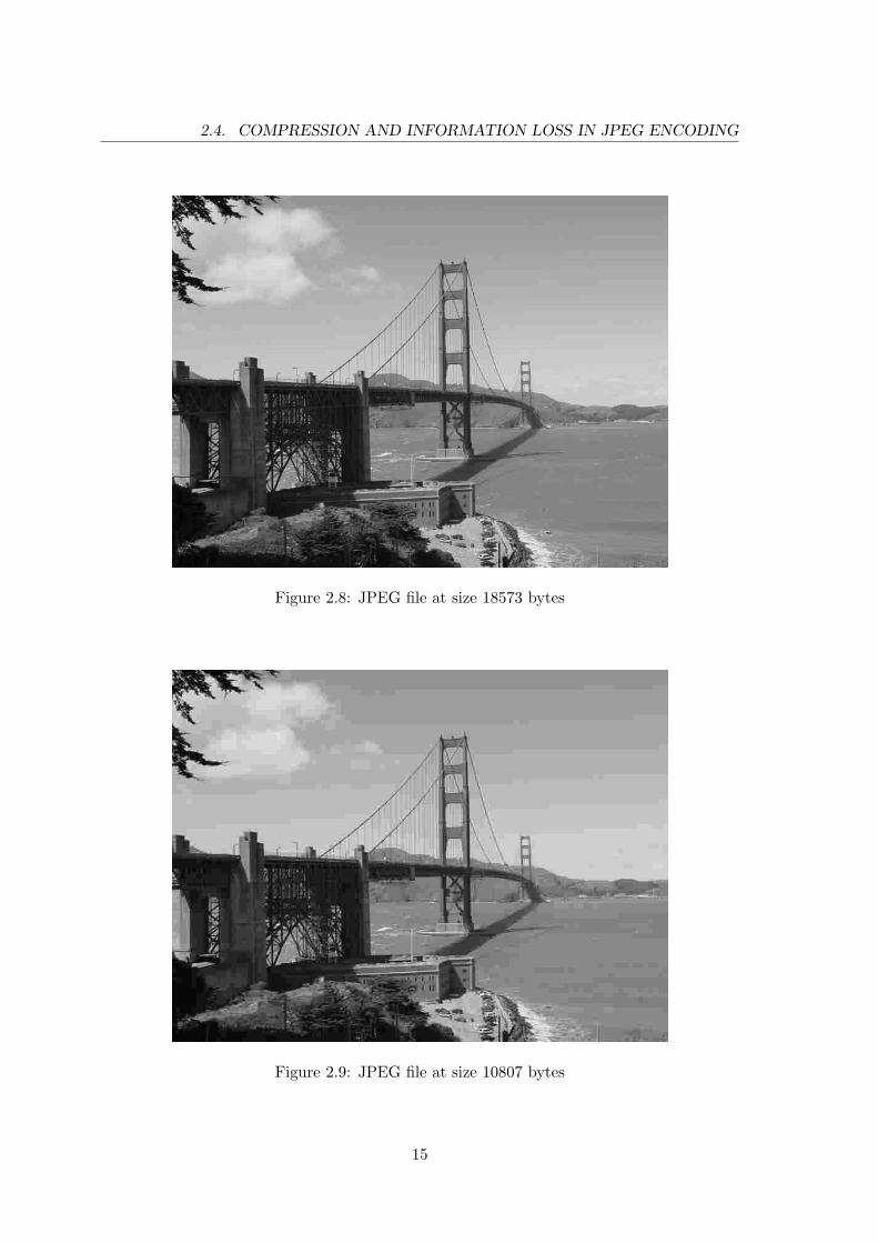
As an example of how the selection of the quantization table affects image quality andcompression, we will look at a greyscale image13 and various compressed variants of it in theJFIF format (all with 4:4:4 chroma subsampling). Figure 2.5 shows the original file with aresolution of 800×600 pixels. Figures 2.6, 2.7, 2.8 and 2.9 show a JPEG-compressed versionat various file sizes (54680 bytes, 35336 bytes, 18573 bytes and 10807 bytes, respectively).
Figure 2.6 uses the following quantization table:
8 6 6 7 6 5 8 77 7 9 9 8 10 12 2013 12 11 11 12 25 18 1915 20 29 26 31 30 29 2628 28 32 36 46 39 32 3444 35 28 28 40 55 41 4448 49 52 52 52 31 39 5761 56 50 60 46 51 52 50
A comparison with the original file in 2.5 shows no real apparent difference while this filehas only about 11 % of the original file’s size. This quantization table already favours thevalues around the DC coefficients, the highest value can be found in the last row (61). Thelowest values are in the upper left corner.
13This image is provided courtesy of Arwed Sienitzki, Sony-Wega Corporation.
13

CHAPTER 2. A BRIEF INTRODUCTION TO JPEG ENCODING AND DECODING
Figure 2.6: JPEG file at size 54680 bytes
Figure 2.7: JPEG file at size 35336 bytes
14
2.4. COMPRESSION AND INFORMATION LOSS IN JPEG ENCODING
Figure 2.8: JPEG file at size 18573 bytes
Figure 2.9: JPEG file at size 10807 bytes
15

CHAPTER 2. A BRIEF INTRODUCTION TO JPEG ENCODING AND DECODING
Figure 2.7 uses the following quantization table:
16 11 12 14 12 10 16 1413 14 18 17 16 19 24 4026 24 22 22 24 49 35 3729 40 58 51 61 60 57 5156 55 64 72 92 78 64 6887 69 55 56 80 109 81 8795 98 103 104 103 62 77 113121 112 100 120 92 101 103 99
Still, only few artifacts can be found in this image, while it has only about 7 % of theoriginal file’s size.
Figure 2.8 uses the following quantization table:
40 28 30 35 30 25 40 3533 35 45 43 40 48 60 10065 60 55 55 60 123 88 9373 100 145 128 153 150 143 128140 138 160 180 230 195 160 170218 173 138 140 200 255 203 218238 245 255 255 255 155 193 255255 255 250 255 230 253 255 248
In this quantization table already lots of table entries have the maximum value of 255, thelowest values are again in the upper left corner. Quite some artifacts can now be seen inthis image, that has about 4 % of the original file’s size.
Figure 2.9 uses the following quantization table:
80 55 60 70 60 50 80 7065 70 90 85 80 95 120 200130 120 110 110 120 245 175 185145 200 255 255 255 255 255 255255 255 255 255 255 255 255 255255 255 255 255 255 255 255 255255 255 255 255 255 255 255 255255 255 255 255 255 255 255 255
In this quantization table only the values in the upper left corner don’t have the maximumvalue of 255. This image is clearly of unæsthetic quality but occupies only about 2 % ofthe original file’s size. In this image also the drawback of grouping pixels into 8× 8 blockscan be seen in that so called “blocking artifacts” appear and the grouping into these blocksbecomes immediately visible to the viewer.
16

Chapter 3
The Discrete Cosine Transform
And when God gave out rhythm,he sure was good to you.You can add, subtract, multiply and divide . . . by two.
– From the song “Popsicle Toes” by Michael Franks, 1976
The Discrete Cosine Transform (DCT) is the transformation that is at the heart of JPEGcompression and decompression. It was proposed in 1972 to the American National
Science Foundation by Nasir Ahmed as an algorithm to achieve bandwidth compression.According to Ahmed, the proposal was not funded because the reviewers found “the wholeidea seemed too simple” [1]. Ahmed continued to work on the DCT together with his Ph.D.student Raj Natarajan and Ram Mohan Rao and published it in a paper ([20]) in 1974.
In applications of the DCT, such as JPEG encoding and decoding, the bandwidth com-pression is achieved by transforming the digital image via the DCT into the DCT FrequencyDomain where those portions of the image that are less important or imperceptible for thehuman eye appear clearly separated from the perceptible features of the image and thuscan be removed. But the DCT is not only relevant for still images like in JPEG, it is alsoan integral part of moving picture standards like MPEG-1 and MPEG-2.
The DCT is also of particular importance for other compression standards, such asDolby AC-3 which is used as the audio compression standard for HDTV, where a modifiedversion of the DCT has been adopted.
This chapter deals with the mathematical definition and gives an overview over severalfast DCT implementations. It also contains a comparison of the DCT and the DiscreteFourier Transform (DFT) that shows that the DCT is a special case of the DFT for a realand symmetrical input vector and how a DFT on a real input vector can be split into severalDFTs and DCTs and vice versa, following a Divide-and-Conquer scheme.
3.1 Mathematical Definition of the DCT
3.1.1 The one-dimensional DCT
The process of transforming a one-dimensional set of N real valued samples into the DCTFrequency Domain is called the forward discrete cosine transform (FDCT) and creates a set
17

CHAPTER 3. THE DISCRETE COSINE TRANSFORM
with the same number of real valued samples which are often called the DCT coefficients.The reverse process that recreates the original image from the DCT coefficients is called theinverse discrete cosine transform (IDCT). The definitions of the N-point FDCT and IDCTare as follows ([20]):
FDCT: F (u) =2N
c(u)N−1∑n=0
f(n) cos(2n + 1) uπ
2N, u = 0, . . . , N − 1 (3.1)
IDCT: f(n) =N−1∑u=0
c(u)F (u) cos(2n + 1) uπ
2N, n = 0, . . . , N − 1 (3.2)
where n, u ∈ N and
c(u) = 1√2
for u = 0c(u) = 1 for u > 0f(n) = 1-D sample valueF (u) = 1-D DCT coefficient
(3.3)
In the following, we will use the definition from ([23]) and ([22]) where the normalizationconstant 2/N of the FDCT is equally distributed over the FDCT and IDCT:
FDCT: F (u) =
√2N
c(u)N−1∑n=0
f(n) cos(2n + 1) uπ
2N, u = 0, . . . , N − 1 (3.4)
IDCT: f(n) =
√2N
N−1∑u=0
c(u)F (u) cos(2n + 1) uπ
2N, n = 0, . . . , N − 1 (3.5)
For JPEG encoding and decoding, the number of samples is always N = 8, so equations(3.4) and (3.5) become equations (3.6) and (3.7):
FDCT: F (u) =c(u)2
7∑n=0
f(n) cos(2n + 1) uπ
16, u = 0, . . . , 7 (3.6)
IDCT: f(n) =7∑
u=0
c(u)2
F (u) cos(2n + 1) uπ
16, n = 0, . . . , 7 (3.7)
The FDCT can be exemplified as a decomposition of an input sample vector into a scaled setof cosine base function vectors with the DCT coefficients as the scaling values. Summing upthe scaled cosine base functions vectors then corresponds to the IDCT process. The DCTas defined in equation (3.4) is an orthonormal transform (see [23]), which simply means,that the inner product of any two different cosine base function vectors is always zero1 and
1Two vector’s inner product is 0 if the vectors are orthogonal, therefore the ortho- in orthonormal trans-form
18
3.1.2. THE TWO-DIMENSIONAL DCT
that the inner product of a cosine base function vector with itself is always one2. Thisalso means, that no cosine base function can be represented by a scaled sum of differentcosine base functions and that all possible input vectors can be represented by a sum ofscaled cosine base function vectors with the scaling values (DCT coefficients) being uniquefor each input vector. In this respect, the Cosine Transform is very similar to the FourierTransform while having the advantage of being a real transform. The obvious similaritiesand relations between the DCT and the Discrete Fourier Transform are covered in chapter3.2. A nice and intuitive introduction into the DCT and its similarities with the FourierTransform can also be found in [2].
3.1.2 The two-dimensional DCT
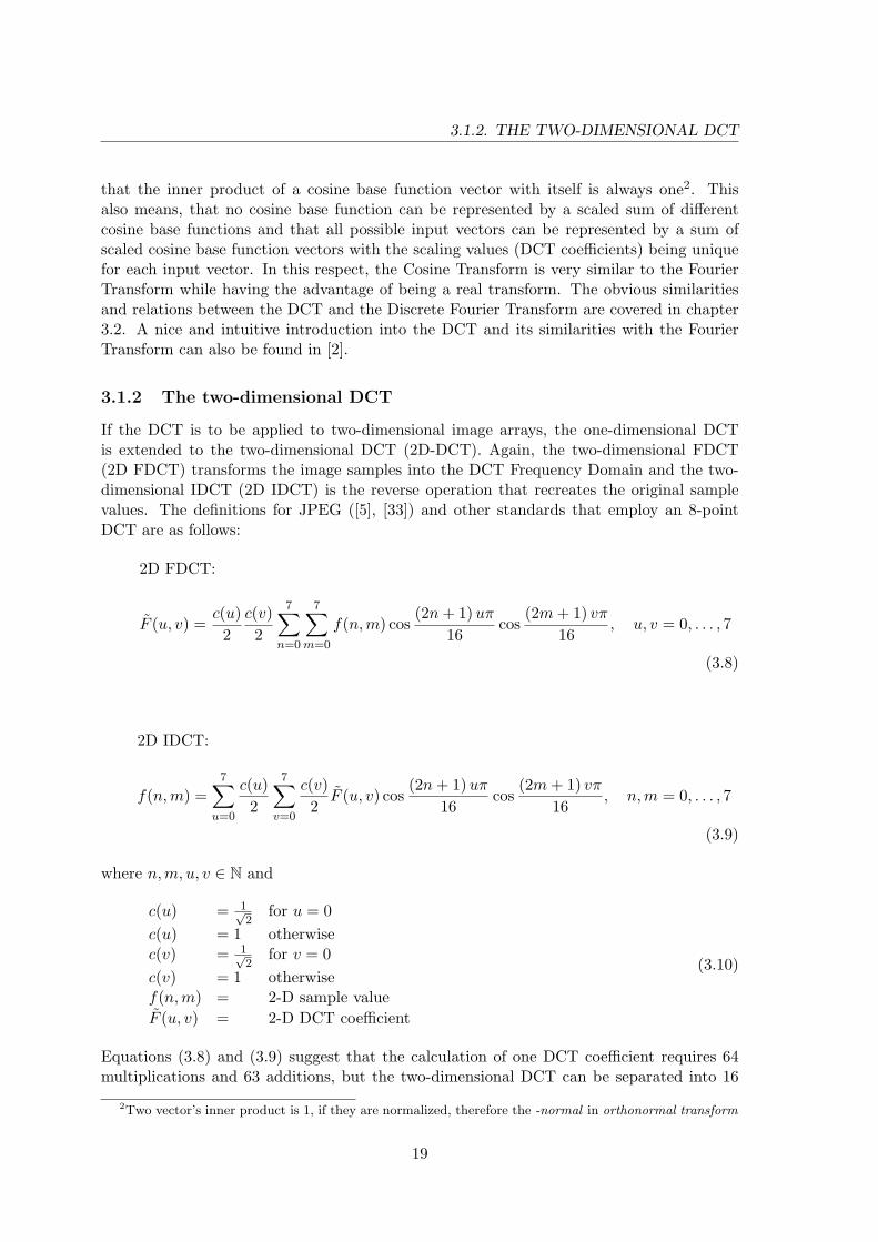
If the DCT is to be applied to two-dimensional image arrays, the one-dimensional DCTis extended to the two-dimensional DCT (2D-DCT). Again, the two-dimensional FDCT(2D FDCT) transforms the image samples into the DCT Frequency Domain and the two-dimensional IDCT (2D IDCT) is the reverse operation that recreates the original samplevalues. The definitions for JPEG ([5], [33]) and other standards that employ an 8-pointDCT are as follows:
2D FDCT:
F (u, v) =c(u)2
c(v)2
7∑n=0
7∑m=0
f(n, m) cos(2n + 1) uπ
16cos
(2m + 1) vπ
16, u, v = 0, . . . , 7
(3.8)
2D IDCT:
f(n, m) =7∑
u=0
c(u)2
7∑v=0
c(v)2
F (u, v) cos(2n + 1) uπ
16cos
(2m + 1) vπ
16, n,m = 0, . . . , 7
(3.9)
where n, m, u, v ∈ N and
c(u) = 1√2
for u = 0c(u) = 1 otherwisec(v) = 1√
2for v = 0
c(v) = 1 otherwisef(n, m) = 2-D sample valueF (u, v) = 2-D DCT coefficient
(3.10)
Equations (3.8) and (3.9) suggest that the calculation of one DCT coefficient requires 64multiplications and 63 additions, but the two-dimensional DCT can be separated into 16
2Two vector’s inner product is 1, if they are normalized, therefore the -normal in orthonormal transform
19

CHAPTER 3. THE DISCRETE COSINE TRANSFORM
one-dimensional DCTs, as (3.11) and (3.12) illustrate:
2D FDCT:
F (u, v) =c(u)2
c(v)2
7∑n=0
(cos
(2n + 1) uπ
16
7∑m=0
f(n, m) cos(2m + 1) uπ
16
), u, v = 0, . . . , 7
(3.11)
2D IDCT:
f(n, m) =7∑
u=0
(c(u)2
cos(2n + 1) uπ
16
7∑v=0
c(v)2
F (u, v) cos(2m + 1) uπ
16
), n,m = 0, . . . , 7
(3.12)
This means, that a two-dimensional DCT can be obtained by applying first 8 one-dimen-sional DCTs over the rows, followed by another 8 one-dimensional DCTs to the columns ofthe input data matrix. Furthermore, there are quite a number of algorithms that reducecomputational complexity drastically. Most of them are based on earlier work done onthe Fast Fourier Transform, that preceeded the DCT about 10 years3, and on the DiscreteFourier Transform in general. Because of the similarities between the Discrete FourierTransform and the DCT it is therefore worthwile looking into the relations between thesetwo orthogonal transforms.
3.2 Relations between the DCT and the DFT
In their introductory paper to the DCT ([20]), Ahmed et al. suggested to use existingFast Fourier Transform algorithms to compute an N-point DCT from a 2N-point DFT.Section 3.2.1 elaborates on their initial proposal. The DCT is also very closely relatedto the Discrete Fourier Transform (DFT) on real inputs (which is the case for 2D imagearrays). This relationship is the basis for the most efficient DCT algorithms known up tonow. Section 3.2.2 shows, how an N-point DFT can be calculated from one N/2-point DFTand two N/4-point DCTs, which is the basis for the Ligtenberg-Vetterli Fast DCT andsimilar algorithms. Section 3.2.3 then shows the relations between the N-point DCT andthe 2N-point DFT for the special case of a symmetrical input vector for the DFT, whichis the basis for the fastest scaled one-dimensional DCT algorithm known up to now, theArai-Agui-Nakajima Fast DCT.
3The famous Cooley-Tukey algorithm ([6]) was presented in 1965
20

3.2.1. COMPUTING AN N-POINT DCT FROM A 2N-POINT DFT
3.2.1 Computing an N-point DCT from a 2N-point DFT
An N-point DFT ([3]) is defined as:
F (u) =N−1∑n=0
f(n)e−j 2πnuN =
N−1∑n=0
f(n)[cos(
2πnu
N
)− j sin
(2πnu
N
)], (3.13)
u = 0, . . . , N − 1
with j =√−1. Consequently, a 2N-point DFT is defined as:
F (u) =2N−1∑n=0
f(n)e−j 2πnu2N , u = 0, . . . , 2N − 1 (3.14)
If we scale equation (3.14)with e−juπ/(2N) and assume that the input samples f(N) . . .f(2N − 1) are zero, we get:
e −j πu2N ·
N−1∑n=0
f(n)e−j 2πnu2N =
N−1∑n=0
f(n)e−juπ(2n+1)
2N
=N−1∑n=0
f(n)(
cos(
uπ(2n + 1)2N
)− j sin
(uπ(2n + 1)
2N
)), u = 0, . . . , 2N − 1
(3.15)
From equation (3.15) and a comparison with equations (3.1) and (3.4) we can deduce,that an N-point DCT can be computed by taking the real part of a 2N-point DFT thatwas scaled by the complex constant e−juπ/(2N). Note that this was an early suggestion ofAhmed et al. in their introductory paper to the DCT ([20]) on how to calculate a DCTleveraging existing algorithms or hardware for the calculation of the DFT. By no means,this calculation method should be considered a particularly efficient one.
3.2.2 A Divide-and-Conquer Scheme for real input vectors
In [32], Vetterli and Nussbaumer present a simple approach to break the task of calculatingan N-point DFT into transformations of reduced complexity for real input vectors. For thispurpose they define two operations, the Cosine DFT and the Sine DFT, that together rep-resent the DFT operation. The Cosine DFT represents the real part of the DFT operation,whereas the Sine DFT represents the imaginary part of the DFT operation. They also usea slightly modified version of the DCT, which, in order to not confuse the reader, is calledDCT* in the following. Vetterli and Nussbaumer also introduce the following notation forthe N-point DFT of a function f(n) which is the same as we already introduced in equation(3.13):
DFT(u,N, f) =N−1∑n=0
f(n)e−j 2πnuN =
N−1∑n=0
f(n)[cos(
2πnu
N
)− j sin
(2πnu
N
)],
u = 0, . . . , N − 1 (3.16)
21

CHAPTER 3. THE DISCRETE COSINE TRANSFORM
with j =√−1. Vetterli and Nussbaumer define the Sine DFT (sin-DFT) and the Cosine
DFT (cos-DFT) as:
sin-DFT(u, N, f) =N−1∑n=0
f(n) sin(
2πnu
N
), u = 0, . . . , N − 1 (3.17)
cos-DFT(u, N, f) =N−1∑n=0
f(n) cos(
2πnu
N
), u = 0, . . . , N − 1 (3.18)
The Sine DFT from equation (3.17) and the Cosine DFT from equation (3.18) togetherconstitute the DFT from equation (3.16):
DFT(u, N, f) = cos-DFT(u, N, f)− j · sin-DFT(u, N, f), u = 0, . . . , N − 1 (3.19)
The DCT* Operation is defined as:
DCT*(u, N, f) =N−1∑n=0
f(n) cos(
2π(2n + 1)u4N
), u = 0, . . . , N − 1 (3.20)
Note that the DCT* in equation (3.20) is just a simplified form of the forward DCT in
equation (3.4) without the scaling of√
2N and the factor 1/
√2 for u = 0. By exploiting
symmetry properties of the Sine and Cosine functions and under the assumption that N isdivisible by 4, equation (3.18) can be rewritten as:
cos-DFT(u, N, f) =N/2−1∑n=0
f(2n) cos(
2πnu
N/2
)(3.21)
+N/4−1∑n=0
(f(2n + 1) + f(N − 2n− 1)) cos2π(2n + 1)u
4N/4,
u = 0, . . . , N − 1
or with f1(n) = f(2n) for n = 0, . . . N/2 − 1 and f2(n) = f(2n + 1) + f(N − 2n − 1) forn = 0, . . . N/4− 1 as:
cos-DFT(u, N, f) = cos-DFT(u, N/2, f1)+DCT*(u, N/4, f2), u = 0 . . . , N − 1 (3.22)
Equation (3.22) shows, that an N-point Cosine DFT can be divided into an N/2-point CosineDFT and an N/4-point DCT*. The N/2-point Cosine DFT can further be subdivided untilonly trivial operations are left. Similarly, the Sine DFT in equation (3.17) can be rewrittenas:
sin-DFT(u, N, f) =N/2−1∑n=0
f(2n) sin(
2πnu
N/2
)(3.23)
+N/4−1∑n=0
(f(2n + 1) + f(N − 2n− 1)) sin2π(2n + 1)u
4N/4,
u = 0, . . . , N − 1
22

3.2.2. A DIVIDE-AND-CONQUER SCHEME FOR REAL INPUT VECTORS
Using the identity:
sin2πn(2n + 1)u
N= (−1)n cos
2π(2n + 1)(N/4− u)N
(3.24)
equation (3.23) can be written in a more succinct form as:
sin-DFT(u, N, f) = sin-DFT(u, N/2, f1)+DCT*(N/4−u,N/4, f3), u = 0 . . . , N−1(3.25)
with f3(n) = (−1)n (f(2n + 1)− f(N − 2n− 1)). Equation (3.25) shows, that an N-pointSine DFT can be subdivided into an N/2 point Sine DFT and an N/4-point DCT*. Togetherwith equation (3.22) this means, that an N-point DFT can be subdivided into one N/2-pointDFT and two N/4-point DCT* operations.
We will now show how to do the reverse process and therefore compute a DCT* operationfrom a Sine DFT and a Cosine DFT:
With the mapping:
f4(n) = f(2n),f4(N − n− 1) = f(2n + 1), n = 0 . . . , N/2− 1
the DCT* in equation (3.20) becomes:
DCT*(u, N, f) =N−1∑n=0
f4(n) cos(
2π(4n + 1)u4N
), u = 0, . . . , N − 1 (3.26)
With the basic geometrical identity cos(α + β) = cos α cos β − sinα sinβ, equation (3.26)becomes:
DCT*(u, N, f) = cos(
2πu
4N
)cos-DFT(u, N, f4)
− sin(
2πu
4N
)sin-DFT(u, N, f4), u = 0, . . . , N − 1
(3.27)
Using the symmetry properties of trigonometric functions and the Sine and Cosine DFT,this can be written as:
(DCT*(u, N, f)
DCT*(N − u, N, f)
)=(
cos(2πu4N ) − sin
(2πu4N
)sin(2πu
4N ) cos(2πu4N )
)(cos-DFT(u,N, f4)sin-DFT(u, N, f4)
)u = 0 . . . , N/2− 1 (3.28)
Equation (3.28) is a rotation of a vector consisting of the real and the imaginary part of theDFT with a rotation angle of 2πu/4N . Thus we have shown how to compute a DCT* (andthus a DCT) from a DFT (equation (3.28)) and vice versa (equations (3.22) and (3.25)). Wewill show in section 3.3.2.1 that this rotation only requires 3 multiplications and 3 additions.In section 3.3.2.2 we will show how to transform this into flowgraphs for an 8-point DCT.
23

CHAPTER 3. THE DISCRETE COSINE TRANSFORM
3.2.3 DCT and DFT for real and symmetrical input vectors
In [29], Tseng and Miller show, that if the mirror image of a sequence of N samples isappended to itself, the first N points of the 2N-point DFT performed on this vector ofsize 2N are scaled values of the DCT coefficients of the original N-point sequence. Theyconclude that an N-point DCT can therefore be very efficiently calculated by taking onedouble length real DFT 4 and a final output scaling, which will be shown in the following.If we use the shortcut WK = e−j 2π
K , the K-point DFT (see equation (3.13)) can be writtenas:
F (u) =K−1∑n=0
f(n)W unK , u = 0, . . . ,K − 1 (3.29)
If we set K = 2N and extend the N-point sequence f(n), n = 0, . . . , N − 1 such that thereis symmetry around the index (2N − 1)/2, we get:
f(n) = f(2N − 1− n), n = 0, . . . , 2N − 1 (3.30)
and equation (3.29) becomes:
F (u) =N−1∑n=0
f(n)W un2N +
2N−1∑n=N
f(2N − n− 1)W un2N , u = 0, . . . , 2N − 1 (3.31)
Now if we define a new index k = (2N − n − 1) for the the second sum in equation (3.31)this becomes:
F (u) =N−1∑n=0
f(n)W un2N +
N−1∑k=0
f(k)W−u(k+1)2N , u = 0, . . . , 2N − 1 (3.32)
If k is now replaced with n and equation (3.32) is multiplied by 12W
u2
2N , we obtain:
12F (u)W
u2
2N =12
N−1∑n=0
f(n)(
Wu2(2n+1)
2N + W−u2
(2n+1)
2N
)
=12
N−1∑n=0
f(n)(e−jπ u
2N(2n+1) + ejπ u
2N(2n+1)
)=
N−1∑n=0
f(n) cosπu
2N(2n + 1), u = 0, . . . , 2N − 1 (3.33)
From equation (3.33) we can deduce that the first N DFT coefficients of a 2N-point DFTare the DCT coefficients of an N point DCT, scaled by a complex scaling factor, providedthat equation (3.30) holds for the input vector.
Our goal will now be to calculate this scaling factor: Since the right side of equation(3.33) is real, the left side must also be real and we therefore can obtain the real part Au
and the imaginary part Bu of F (u) with:
F (u)Wu2
2N = (Au + jBu)(cosπu
2N− j sin
πu
2N), u = 0, . . . , 2N − 1 (3.34)
4A real DFT denotes a DFT with real input, in contrast to a complex DFT with a complex input vector
24

3.3. FAST ONE-DIMENSIONAL 8-POINT DCTS
Separating equation (3.34) into a real and an imaginary parts and setting the imaginarypart to zero we get:
Bu = Ausin πu
2N
cos πu2N
(3.35)
which can be substituted back into equation (3.34):
F (u)Wu2
2N = Au cosπu
2N+ Au
sin2 πu2N
cos πu2N
= Au1
cos πu2N
(cos2πu
2N+ sin2 πu
2N)
= Au1
cos πu2N
, u = 0, . . . , 2N − 1 (3.36)
From equations (3.33) and (3.36) we now get:
N−1∑n=0
f(n) cosπu
2N(2n + 1) =
12<(F (u))
1cos πu
2N
, u = 0, . . . , 2N − 1 (3.37)
This shows that the DCT coefficients of an N-point DCT can simply be derived from scalingthe real part of a 2N-point DFT with symmetrical input vector. Chapter 3.3.6 will showthat for N = 8 this property is the basis of the Arai-Agui-Nakajima Fast DCT.
3.3 Fast one-dimensional 8-point DCTs
This section will cover in detail several fast one-dimensional DCT algorithms that havebeen developed over the years both for software and hardware implementations. Becauseof the widespread use of 8-point DCTs and IDCTs in continuous tone image encoding anddecoding, we will strictly focus on algorithms for an 8-point input vector. This also meansthat we don’t evaluate the complexity of algorithms in terms of ”Big-Oh-Notation”, such asO(N), O(N2), O(logN), because N = 8 is a fixed value. We rather compare algorithms byevaluating the number of additions and multiplications they require. In order to describethe algorithms a graphical notation, the flowgraph, will be introduced. We will start witha very simple 8-point DCT, taken from [22], that demonstrates how the symmetry of thesine and cosine function can be exploited to reduce computational complexity of the DCT.We will then proceed in section 3.3.2 to the first classical DCT algorithm, the Ligtenberg-Vetterli DCT (1986), that we analyze first with an algebraic approach (section 3.3.2.1) andthen with a more graphical and intuitive approach (section 3.3.2.2). From there we willturn to the Loeffler-Ligtenberg-Moschytz DCT (1989) and its inverse, which is the fastestunscaled one-dimensional DCT known up to now. The section on fast one-dimensional8-point DCTs is then concluded with section 3.3.6 that contains an analysis of the Arai-Agui-Nakajima Fast DCT (1988) and its inverse, which is the fastest scaled one-dimensionalDCT known up to now. For this algorithm the “Winograd 16-point small-N DFT” is ofparticular importance. Therefore we will analyze this algorithm as well.
25

CHAPTER 3. THE DISCRETE COSINE TRANSFORM
3.3.1 A simple and fast 8-point DCT
A simple approach ([22]) for a fast DCT takes advantage of the symmetry of sinusoidalfunctions. With the following definitions:
Ck = coskπ
16, Sk = sin
kπ
16, k = 0, . . . , 7 (3.38)
we get from the symmetry property of the cosine and sine functions:
C1 = S7, C2 = S6, ..., C7 = S1 (3.39)
and
C1 = −C15, C2 = −C14, ..., C7 = −C9. (3.40)
We therefore define the following shortcuts for sums (3.41) and differences (3.42) of thesamples f(n):
s07 = f(0) + f(7)s16 = f(1) + f(6)s25 = f(2) + f(5)s34 = f(3) + f(4)s0734 = s07 + s34
s1625 = s16 + s25
(3.41)
d07 = f(0)− f(7)d16 = f(1)− f(6)d25 = f(2)− f(5)d34 = f(3)− f(4)d0734 = s07 − s34
d1625 = s16 − s25
(3.42)
With the shortcuts from equations (3.41) and (3.42), the DCT coefficients from (3.6) canbe written as:
2F (0) =1√2
7∑n=0
f(n) cos(0) = cos4π
16
7∑n=0
f(n) = C4(s0734 + s1625) (3.43)
2F (1) = cosπ
16f(0) + cos
3π
16f(1) + cos
5π
16f(2) + cos
7π
16f(3)
+ cos9π
16f(4) + cos
11π
16f(5) + cos
13π
16f(6) + cos
15π
16f(7)
= cosπ
16[f(0)− f(7)] + cos
3π
16[f(1)− f(6)]
+ cos5π
16[f(2)− f(5)] + cos
7π
16[f(3)− f(4)]
= C1d07 + C3d16 + C5d25 + C7d34 (3.44)
26

3.3.1. A SIMPLE AND FAST 8-POINT DCT
2F (2) = cos2π
16f(0) + cos
6π
16f(1) + cos
10π
16f(2) + cos
14π
16f(3)
+ cos18π
16f(4) + cos
22π
16f(5) + cos
26π
16f(6) + cos
30π
16f(7)
= cos2π
16[f(0) + f(7)− f(3)− f(4)]
+ cos6π
16[f(1) + f(6)− f(2)− f(5)]
= C2d0734 + C6d1625 (3.45)
2F (3) = cos3π
16f(0) + cos
9π
16f(1) + cos
15π
16f(2) + cos
21π
16f(3)
+ cos27π
16f(4) + cos
33π
16f(5) + cos
39π
16f(6) + cos
45π
16f(7)
= cos3π
16[f(0)− f(7)]− cos
7π
16[f(1)− f(6)]
+ cos7π
16[f(2)− f(5)]− cos
5π
16[f(3)− f(4)]
= C3d07 − C7d16 − C1d25 − C5d34 (3.46)
2F (4) = cos4π
16f(0) + cos
12π
16f(1) + cos
20π
16f(2) + cos
28π
16f(3)
+ cos36π
16f(4) + cos
44π
16f(5) + cos
52π
16f(6) + cos
60π
16f(7)
= cos4π
16[f(0) + f(3) + f(4) + f(7)− f(1)− f(2)− f(5)− f(6)]
= C4(s0734 − s1625) (3.47)
2F (5) = cos5π
16f(0) + cos
15π
16f(1) + cos
25π
16f(2) + cos
35π
16f(3)
+ cos45π
16f(4) + cos
55π
16f(5) + cos
65π
16f(6) + cos
75π
16f(7)
= cos5π
16[f(0)− f(7)]− cos
π
16[f(1)− f(6)]
+ cos7π
16[f(2)− f(5)] + cos
3π
16[f(3)− f(4)]
= C5d07 − C1d16 + C7d25 + C3d34 (3.48)
2F (6) = cos6π
16f(0) + cos
18π
16f(1) + cos
30π
16f(2) + cos
42π
16f(3)
+ cos54π
16f(4) + cos
66π
16f(5) + cos
78π
16f(6) + cos
90π
16f(7)
= cos6π
16[f(0) + f(7)− f(3)− f(4)] + cos
2π
16[f(2) + f(5)− f(1)− f(6)]
= C6d0734 − C2d1625 (3.49)
27

CHAPTER 3. THE DISCRETE COSINE TRANSFORM
2F (7) = cos7π
16f(0) + cos
21π
16f(1) + cos
35π
16f(2) + cos
49π
16f(3)
+ cos63π
16f(4) + cos
77π
16f(5) + cos
91π
16f(6) + cos
105π
16f(7)
= cos7π
16[f(0)− f(7)]− cos
5π
16[f(1)− f(6)]
+ cos3π
16[f(2)− f(5)]− cos
π
16[f(3)− f(4)]
= C7d07 − C5d16 + C3d25 − C1d34 (3.50)
By arranging the terms in equations (3.43)-(3.50), the sums and differences from equations(3.41) and (3.42) can be reused to calculate the DCT coefficients and thus the total amountof operations is reduced to 22 multiplications and 28 additions. This is quite some progress,compared to the naıve approach of calculating each of the 8 coefficients by 7 additions and8 multiplications.
3.3.2 The Ligtenberg-Vetterli-DCT
In this section an algorithm is presented that was introduced by Ligtenberg and Vetterliand implemented in hardware as early as 1986 ([31]). It employs the Divide-and-Conquerscheme presented in section 3.2.2. We will first use in section 3.3.2.1 the algebraic approachfrom [22], which should be enough to successfully implement this algorithm and requires noprior understanding of section 3.2.2. Section 3.3.2.2 will then use a more intuitive approachand will show how to graphically derive a flowgraph for this algorithm based on chapter3.2.2.
3.3.2.1 An algebraic approach to the Ligtenberg-Vetterli-DCT
The Ligtenberg-Vetterli-DCT uses equations (3.43)-(3.50) and the sums and differencesfrom equations (3.41) and (3.42), but with slightly different grouping:
2F (0) = C4 [(s07 + s12) + (s34 + s56)] (3.51)
2F (1) = C1d07 + C3d16 + C5d25 + C7d34
= (C1d07 + S1d34) + (C3d16 + S3d25) (3.52)
2F (2) = C2(s07 − s34) + C6(d12 − d56)= C6(d12 − d56) + S6(s07 − s34) = C−6(d12 − d56)− S−6(s07 − s34) (3.53)
2F (3) = C3d07 − (C5d34 + C7d16 + C1d25)= (C3d07 − S3d34)− (S1d16 + C1d25) (3.54)
2F (4) = C4 [(s07 + s34)− (s12 + s56)] (3.55)
2F (5) = C5d07 + C7d25 + C3d34 − C1d16
= (S3d07 + C3d34) + (S1d25 − C1d16) (3.56)
28

3.3.2.1. AN ALGEBRAIC APPROACH TO THE LIGTENBERG-VETTERLI-DCT
2F (6) = C6(s07 − s34) + C2(s25 − s16)= −S6(d12 − d56) + C6(s07 − s34) = S−6(d12 − d56) + C−6(s07 − s34) (3.57)
2F (7) = C7d07 + C3d25 − (C5d16 + C1d34)= (S1d07 − C1d34) + (C3d25 − C5d16) (3.58)
From the standard geometric identities
cos α− cos β = −2 sinα + β
2sin
α− β
2(3.59)
and
cos α + cos β = 2 cosα + β
2cos
α− β
2(3.60)
we get for k, l ∈ N:
Ck − Cl = −2sin(k + l)π
32sin
(k − l)π32
= −2S(k+l)/2S(k−l)/2 (3.61)
Ck + Cl = 2cos(k + l)π
32cos
(k − l)π32
= 2C(k+l)/2C(k−l)/2 (3.62)
From (3.51) and (3.55) we can deduce, that F (0) and F (4) can be calculated very straight-forward by simple additions and a multiplication. For all other DCT coefficients, theLigtenberg-Vetterli Fast DCT employs the rotation operation, that was introduced in sec-tion 3.2.2. The rotation operation rotates two input values (x, y) to output values (X, Y )by an angle Θ using the following equations:
X = x cos Θ− y sinΘ (3.63)
Y = x sinΘ + y cos Θ (3.64)
For a rotation angle Θ = kπ16 , equations (3.63) and (3.64) become:
X = Ckx− Sky (3.65)
Y = Skx + Cky (3.66)
which can be expressed as:
X = Ck(x + y)− (Sk + Ck)y (3.67)
Y = (Sk − Ck)x + Ck(x + y) (3.68)
29

CHAPTER 3. THE DISCRETE COSINE TRANSFORM
with Sk and Ck defined as in equation (3.38). Note that equations (3.65) and (3.66) requirefour multiplications and two additions whereas equations (3.67) and (3.68) require onlythree multiplications and three additions (Sk ±Ck are constants that can be precalculated)which is advantageous if a multiplication is costlier than an addition on a given computerhardware.
From (3.53) and (3.57) we can see that calculating 2F (2) and 2F (6) is simply a rotationof the inputs x = (d12 − d56) and y = (s07 − s34) with a rotation angle of Θ = −6π
16 . Inorder to calculate the other DCT coefficients with a rotation, some additional recasting isrequired to bring the terms for the DCT coefficients into a form that is suitable for therotation operation:
For F (3), the term (S1d16 + C1d25) in (3.54) can be expressed in terms of a sum ofs12, d12, s56 and d56 with four unknown coefficients A, B, C and D:
S1d16 + C1d25 = As12 + Bd12 + Cs56 + Dd56 (3.69)
Solving the coefficients with four separate equations for f(1), f(2), f(5) and f(6) yields:
f(1) : S1 = A + Bf(2) : C1 = A−Bf(5) : −C1 = C + Df(6) : −S1 = C −D
(3.70)
Adding and subtracting the equations in (3.70) the unknown coefficients A, B, C and Dbecome:
A = 12(S1 + C1) = 1
2(C7 + C1) = C4C3
B = 12(S1 − C1) = 1
2(C7 − C1) = −S4S3 = −C4S3
C = −12(C1 + S1) = −1
2(C7 + C1) = −C4C3
D = 12(S1 − C1) = 1
2(C7 − C1) = −S4S3 = −C4S3
(3.71)
With (3.71) the term (S1d16 + C1d25) can be expressed as:
S1d16 + C1d25 = C4 [C3(s12 − s56)− S3(d12 + d56)] (3.72)
and thus (3.54) becomes:
2F (3) = [C3d07 − S3d34]− C4 [C3(s12 − s56)− S3(d12 + d56)] (3.73)
For F (5) we again express the term (S1d25−C1d16) in (3.56) in terms of a sum of s12, d12, s56
and d56 with four unknown coefficients A, B, C and D:
S1d25 − C1d16 = As12 + Bd12 + Cs56 + Dd56 (3.74)
Solving the coefficients with four separate equations for f(1), f(2), f(5) and f(6) yields:
f(1) : −C1 = A + Bf(2) : S1 = A−Bf(5) : −S1 = C + Df(6) : C1 = C −D
(3.75)
30

3.3.2.1. AN ALGEBRAIC APPROACH TO THE LIGTENBERG-VETTERLI-DCT
Again, adding and subtracting the equations in (3.75) the unknown coefficients A, B, Cand D become:
A = −12(C1 − S1) = 1
2(C7 − C1) = −S4S3 = −C4S3
B = −12(C1 + S1) = −1
2(C1 + C7) = −C4C3
C = −12(S1 − C1) = −1
2(C7 − C1) = S4S3 = C4S3
D = −12(S1 + C1) = −1
2(C7 + C1) = −C4C3
(3.76)
With (3.76) the term S1d25 − C1d16 can be expressed as:
S1d25 − C1d16 = C4 [−S3(s12 − s56)− C3(d12 + d56)] (3.77)
and thus (3.56) becomes:
2F (5) = [S3d07 + C3d34] + C4 [−S3(s12 − s56)− C3(d12 + d56)] (3.78)
Rearranging equations (3.73) and (3.78) gives:
2F (3) = C3 [d07 − C4(s12 − s56)]− S3 [d34 − C4(d12 + d56)]2F (5) = S3 [d07 − C4(s12 − s56)] + C3 [d34 − C4(d12 + d56)]
(3.79)
which is a rotation of x = d07 − C4(s12 − s56) and y = d34 − C4(d12 + d56) with a rotationangle of Θ = 3π
16 .The two remaining DCT coefficients, F (1) and F (7), can be calculated in a similar way
to F (3) and F (5):First the term (C3d16 + S3d25) in (3.52) is expressed in terms of a sum of s12, d12, s56
and d56 with four unknown coefficients A, B, C and D:
C3d16 + S3d25 = As12 + Bd12 + Cs56 + Dd56 (3.80)
Solving the coefficients with four separate equations for f(1), f(2), f(5) and f(6) yields:
f(1) : C3 = A + Bf(2) : S3 = A−Bf(5) : −S3 = C + Df(6) : −C3 = C −D
(3.81)
Again, adding and subtracting the equations in (3.81) the unknown coefficients A, B, Cand D become:
A = 12(C3 + S3) = 1
2(C3 + C5) = C4C1
B = 12(C3 − S3) = −1
2(C5 − C3) = S4S1 = C4S1
C = −12(S3 + C3) = −1
2(C5 + C3) = −C4C1
D = −12(S3 − C3) = −1
2(C5 − C3) = S4S1 = C4S1
(3.82)
With (3.82) the term C3d16 + S3d25 can be expressed as:
C3d16 + S3d25 = C4 [C1(s12 − s56) + S1(d12 + d56)] (3.83)
and thus (3.52) becomes:
2F (1) = (C1d07 + S1d34) + C4 [C1(s12 − s56) + S1(d12 + d56)] (3.84)
31

CHAPTER 3. THE DISCRETE COSINE TRANSFORM
For S(7) we again express the term (C3d25−C5d16) in (3.58) in terms of a sum of s12, d12, s56
and d56 with four unknown coefficients A, B, C and D:
C3d25 − C5d16 = As12 + Bd12 + Cs56 + Dd56 (3.85)
Solving the coefficients with four separate equations for f(1), f(2), f(5) and f(6) yields:
f(1) : −C5 = A + Bf(2) : C3 = A−Bf(5) : −C3 = C + Df(6) : C5 = C −D
(3.86)
Again, adding and subtracting the equations in (3.86) the unknown coefficients A, B, Cand D become:
A = 12(C3 − C5) = S4S1 = C4S1
B = −12(C5 + C3) = −C4C1
C = 12(C5 − C3) = −S4S1 = −C4S1
D = −12(C5 + C3) = −C4C1
(3.87)
With (3.87) the term C3d25 − C5d16 can be expressed as:
C3d25 − C5d16 = C4 [S1(s12 − s56)− C1(d12 + d56)] (3.88)
and thus (3.58) becomes:
2F (7) = (S1d07 − C1d34) + C4 [S1(s12 − s56)− C1(d12 + d56)] (3.89)
Rearranging equations (3.84) and (3.89) gives:
2F (1) = C1 [d07 + C4(s12 − s56)]− S1 [−d34 − C4(d12 + d56)]2F (7) = S1 [d07 + C4(s12 − s56)] + C1 [−d34 − C4(d12 + d56)]
(3.90)
which is a rotation of x = d07 + C4(s12− s56) and y = −d34−C4(d12 + d56) with a rotationangle of Θ = π
16 .We can now calculate the 8 point DCT with 3 rotations (9 multiplications), the two
multiplications from equations (3.51) and (3.55) and another two multiplications of C4 with(d12 + d56) and (s12− s56) which serve as an input for the rotations in equations (3.79) and(3.90). The total number of operations sums up to 13 multiplications and 29 additions,which will become much more obvious in section 3.3.2.2.
3.3.2.2 A graphical approach to the Ligtenberg-Vetterli-DCT
In this section, we will take a more intuitive approach to the computation of the Ligtenberg-Vetterli DCT than in the preceeding chapter:
If an N point real DFT or a DCT* operation is simply considered a “black box” with Ninput values and N output values, equations (3.22) and (3.25) can be described graphicallylike in figure 3.1 for N = 8. Such a flowgraph is to be read from left to right, a filled dotrepresents an addition of two values and an arrow represents a negation of a value 5. The
5A hollow dot represents the reuse of a value for more than one following operation and thus is not reallyan operation that contributes to computational complexity.
32

3.3.2.2. A GRAPHICAL APPROACH TO THE LIGTENBERG-VETTERLI-DCT
f(0)
f(1)
f(2)
f(3)
f(4)
f(5)
f(6)
f(7)
ℜ( )F(0)
ℜ( )F(1)
ℜ( )F(2)
ℑ( )F(1)
ℜ( )F(4)
ℜ( )F(3)
ℑ( )F(2)
ℑ( )F(1)
4 pt.DFT
2 pt.DCT*
2 pt.DCT*
f'(0)
f'(1)
f'(2)
f'(3)
ℜ( )F'(0)
ℜ( )F'(1)
ℜ( )F'(2)
ℑ( )F'(1)
f''(0)
f''(1)
F*''(0)
F*''(1)
f'(0)
f'(1)
F*'(0)
F*'(1)
~
~
~
~
Figure 3.1: A graphical description of an 8 point real DFT
33

CHAPTER 3. THE DISCRETE COSINE TRANSFORM
f(0)
f(1)
f(2)
f(3)
f(4)
f(5)
f(6)
f(7)
8 pt.DFT
Rot
Rot
Rot
2π16
π16
3π16
C4
F*(0)
F*(1)
F*(2)
F*(3)
F*(4)
F*(5)
F*(6)
F*(7)
ℜ{ }F''(0)
ℜ{ }F''(1)
ℜ{ }F''(2)
ℜ{ }F''(3)
ℜ{ }F''(4)
ℑ{ }F''(1)
ℑ{ }F''(2)
ℑ{ }F''(3)
f''(0)
f''(1)
f''(2)
f''(3)
f''(4)
f''(5)
f''(6)
f''(7)
~
~
~
~
~
~
~
~
Figure 3.2: A graphical description of an 8 point DCT*
astute reader might object at this point that an N-point DFT should yield an N-point realpart and an N-point imaginary part, but it can be easily shown, that for a real input signalfunction the Fourier Transform yields an even function for its real part and an odd functionfor its imaginary part. Therefore
={F (0)} = sin-DFT(0, N, f) = 0 (3.91)
and
={F (N/2)} = sin-DFT(N/2, N, f) = 0 (3.92)
and
={F (u)} = sin-DFT(u, N, f) = -sin-DFT(N − u, N, f) = −={X(N − u)} . (3.93)
Similarly, for the real part, we can find
<{F (u)} = cos-DFT(u, N, f) = cos-DFT(N − u, N, f) = <{F (N − u)} . (3.94)
This reduces the total number of distinct and nonzero values of the N-point real DFT to Nvalues.
The computation of a DCT* from a DFT with rotation operations, as expressed inequation (3.28), can be described graphically like in figure 3.2 for N = 8. In this flowgraph,a box labeled with Rotnπ
16 denotes a rotation operation of the two input values as in equation
34

3.3.2.2. A GRAPHICAL APPROACH TO THE LIGTENBERG-VETTERLI-DCT
f(0)
f(1)
f(2)
f(3)
f(4)
f(5)
f(6)
f(7)
2 ·F (0 )
2 · F ( 3 )
2 ·F (4 )
2 ·F (2 )
2 ·F (6 )
2 ·F (1 )
2 ·F ( 7 )
2 · F ( 5 )
C4
C4
C4
C4 Rot
Rot
Rot2 π1 6
π1 6
3 π1 6
~
~
~
~
~
~
~
~
Figure 3.3: A combination of figures 3.1 and 3.2 to derive the DCT from the DCT*
(3.28) with a rotation angle of nπ/16. A box labeled C4 represents a multiplication withC4 = 1/
√2. In order to not confuse the reader, the output vector of the DCT* in figure
3.2 is denoted F ∗(0) . . . F ∗(7). If the two figures 3.1 and 3.2 are cleverly combined, suchthat the black box labeled “8-pt. DFT” in figure 3.2 is replaced by the complete flowgraphin figure 3.1, it is very easy to derive a flowgraph for the DCT* and finally, for the DCT,like in figure (3.3). Note that we have to add an additional multiplication with C4 forS(0) in order to derive the DCT from the DCT*. From figure (3.3), some optimizationin the number of required negations leads to the flowgraph in figure 3.4. As can be easilyseen from the flowgraph in figure 3.4, the computational complexity of the Ligtenberg-Vetterli-DCT sums up to a total of 13 multiplications and 29 additions. Note that onerotation takes 3 multiplications and 3 additions. The output of the flowgraph is 2 timesthe value of the DCT coefficients, but the required division by 2 can easily be done by aright shift operation which is negligible in computation costs, compared to an addition or amultiplication. In figure 3.4 the boxes for the rotation operation get additional designatorswhere a minus sign means a negation of the input value. Such a negation of a rotation’sinput vector does not contribute to computational complexity, since it can be absorbedinto the precalculated constants of the rotation operation. Ligtenberg and Vetterli actuallysacrificed some computational complexity for the sake of a simpler design of their chip.Figure 3.5 shows the flowgraph for their final design where one “butterfly”-operation (2additions) in the third stage and the two multiplications by 1/
√2 in the last stage are
replaced by a single rotation with a rotation angle of 4π/16 (three multiplications, three
35

CHAPTER 3. THE DISCRETE COSINE TRANSFORM
f(0)
f(1)
f(2)
f(3)
f(4)
f(5)
f(6)
f(7)
2·F(0)
2·F(3)
2·F(4)
2·F(2)
2·F(6)
2·F(1)
2·F(7)
2·F(5)
C4
C4
C4
C4
+
-
+
+
+
+
Rot
Rot
Rot− 6 π
16
π16
3π16
~
~
~
~
~
~
~
~
Figure 3.4: Flowgraph for the Ligtenberg-Vetterli Fast DCT
36

3.3.2.2. A GRAPHICAL APPROACH TO THE LIGTENBERG-VETTERLI-DCT
f(0)
f(1)
f(2)
f(3)
f(4)
f(5)
f(6)
f(7)
2·F(0)
2·F(3)
2·F(4)
2·F(2)
2·F(6)
2·F(1)
2·F(7)
2·F(5)
C4
C4
+
-
+
+
+
+
Rot
Rot
Rot− 6 π
16
π16
3π16
+
+
Rot4π16
~
~
~
~
~
~
~
~
Figure 3.5: Hardware implementation of the Ligtenberg-Vetterli Fast DCT
37

CHAPTER 3. THE DISCRETE COSINE TRANSFORM
f(0)
f(1)
f(2)
f(3)
f(4)
f(5)
f(6)
f(7)
2
2
Rot− 3 π
1 6
Rot− π1 6
2 · R o t− 6 π
1 6
2· 2 ·F(0)~
2· 2 ·F(4)~
2· 2 ·F(2)~
2· 2 ·F(6)~
2· 2 ·F(7)~
2· 2 ·F(3)~
2· 2 ·F(5)~
2· 2 ·F(1)~
Figure 3.6: Flowgraph for the Loeffler-Ligtenberg-Moschytz Fast DCT
additions). Note that a software implementation of their algorithm should preferrably usethe flowgraph in figure 3.4 instead of the flowgraph in figure 3.5.
3.3.3 The Loeffler-Ligtenberg-Moschytz-DCT
In [4], Loeffler et al. present an 8-point DCT algorithm that needs only 11 multiplicationsand 29 additions. Figure 3.6 shows the flowgraph of this algorithm. This algorithm usesthe same kind of rotation as in equations (3.65) and (3.66), denoted by a box labeled withRotΘ, with Θ being the rotation angle. The rotation in the third stage with a rotationangle of −6π
16 is additionally scaled by√
2, therefore it is labeled√
2Rot−6π16 . Note that
this scaling can be absorbed into the constants of the rotation operation and therefore doesnot contribute to computational complexity. The output of this algorithm is scaled to 2
√2
times the DCT coefficients of the input vector, but after a 2D DCT with a total scaling of4√
2√
2, this can easily be reverted by a single right shift operation for each coefficient.
The Loeffler-Ligtenberg-Moschytz Fast DCT can now be written as a matrix-vector
38

3.3.3. THE LOEFFLER-LIGTENBERG-MOSCHYTZ-DCT
product:
F (0)F (1)F (2)F (3)F (4)F (5)F (6)F (7)
=
12√
2·
1 0 0 0 0 0 0 00 0 0 0 0 0 0 10 0 1 0 0 0 0 00 0 0 0 0 1 0 00 1 0 0 0 0 0 00 0 0 0 0 0 1 00 0 0 1 0 0 0 00 0 0 0 1 0 0 0
·
1 0 0 0 0 0 0 00 1 0 0 0 0 0 00 0 1 0 0 0 0 00 0 0 1 0 0 0 00 0 0 0 −1 0 0 10 0 0 0 0
√2 0 0
0 0 0 0 0 0√
2 00 0 0 0 1 0 0 1
·
1 1 0 0 0 0 0 01 −1 0 0 0 0 0 00 0
√2C6
√2S6 0 0 0 0
0 0 −√
2S6
√2C6 0 0 0 0
0 0 0 0 1 0 1 00 0 0 0 0 −1 0 10 0 0 0 1 0 −1 00 0 0 0 0 1 0 1
·
1 0 0 1 0 0 0 00 1 1 0 0 0 0 00 1 −1 0 0 0 0 01 0 0 −1 0 0 0 00 0 0 0 C3 0 0 S3
0 0 0 0 0 C1 S1 00 0 0 0 0 −S1 C1 00 0 0 0 −S3 0 0 C3
·
1 0 0 0 0 0 0 10 1 0 0 0 0 1 00 0 1 0 0 1 0 00 0 0 1 1 0 0 00 0 0 1 −1 0 0 00 0 1 0 0 −1 0 00 1 0 0 0 0 −1 01 0 0 0 0 0 0 −1
·
f(0)f(1)f(2)f(3)f(4)f(5)f(6)f(7)
(3.95)
In [4], Loeffler et al. show, that algorithms like the Ligtenberg-Vetterli-DCT, whichallow the parallel execution of multiplications within one stage, will always take at least 12multiplications, whereas their own algorithm belongs to a class of algorithms that uses acascaded multiplication in one stage but therefore needs one multiplication less. Note thatin [4] the scaled rotation in stage 3 of figure 1 is wrong. It should read
√2 c6 instead of√
2 c1. Note also, that Loeffler, Ligtenberg and Moschytz omitted a scaling factor of√
2 inall constants used in figure 8 in [4], section 4.3.
In [15], an excellent introduction into this algorithm and how to translate it into sourcecode, along with performance figures for different DCT implementations, can be found. TheC source code that accompanies this article is available electronically from the website ofDr. Dobb’s Journal (http://www.ddj.com).
39

CHAPTER 3. THE DISCRETE COSINE TRANSFORM
3.3.4 The Inverse Loeffler-Ligtenberg-Moschytz-DCT
The Inverse Loeffler-Ligtenberg-Moschytz-DCT can easily be derived by simply reversingthe order of matrices in equation (3.95) and inverting the matrices as well. The InverseLoeffler-Ligtenberg-Moschytz-DCT can then be given as:
f(0)f(1)f(2)f(3)f(4)f(5)f(6)f(7)
=
12√
2·
1 0 0 0 0 0 0 10 1 0 0 0 0 1 00 0 1 0 0 1 0 00 0 0 1 1 0 0 00 0 0 1 −1 0 0 00 0 1 0 0 −1 0 00 1 0 0 0 0 −1 01 0 0 0 0 0 0 −1
·
1 0 0 1 0 0 0 00 1 1 0 0 0 0 00 1 −1 0 0 0 0 01 0 0 −1 0 0 0 00 0 0 0 C3 0 0 −S3
0 0 0 0 0 C1 −S1 00 0 0 0 0 S1 C1 00 0 0 0 S3 0 0 C3
·
1 1 0 0 0 0 0 01 −1 0 0 0 0 0 00 0
√2C6 −
√2S6 0 0 0 0
0 0√
2S6
√2C6 0 0 0 0
0 0 0 0 1 0 1 00 0 0 0 0 −1 0 10 0 0 0 1 0 −1 00 0 0 0 0 1 0 1
·
1 0 0 0 0 0 0 00 1 0 0 0 0 0 00 0 1 0 0 0 0 00 0 0 1 0 0 0 00 0 0 0 −1 0 0 10 0 0 0 0
√2 0 0
0 0 0 0 0 0√
2 00 0 0 0 1 0 0 1
·
1 0 0 0 0 0 0 00 0 0 0 1 0 0 00 0 1 0 0 0 0 00 0 0 0 0 0 1 00 0 0 0 0 0 0 10 0 0 1 0 0 0 00 0 0 0 0 1 0 00 1 0 0 0 0 0 0
·
F (0)F (1)F (2)F (3)F (4)F (5)F (6)F (7)
(3.96)
From equation (3.96) it is very easy to derive a a flowgraph which is depicted in figure 3.7.Notice that the rotations simply changed their signs and the stages of the algorithm havejust been mirrored horizontally.
40

3.3.4. THE INVERSE LOEFFLER-LIGTENBERG-MOSCHYTZ-DCT
F(0)
F(4)
F(2)
F(6)
F(7)
F(3)
F(5)
F(1)
2
2
Rot3 π1 6
Rotπ
1 6
2 · R o t6 π1 6
2 · 2 · f (0 )
2 · 2 · f (1 )
2 · 2 · f (2 )
2 · 2 · f (3 )
2 · 2 · f (4 )
2 · 2 · f (5 )
2 · 2 · f (6 )
2 · 2 · f (7 )
~
~
~
~
~
~
~
~
Figure 3.7: Inverse Loeffler-Ligtenberg-Moschytz Fast DCT
41

CHAPTER 3. THE DISCRETE COSINE TRANSFORM
3.3.5 The Winograd 16-point “small-N” DFT
In [34], Shmuel Winograd presented his research work at the IBM Thomas J. WatsonResearch Center on the calculation of Fourier Transforms of arbitrary lengths6. His ideawas to break up the sample length N of the Fourier Transform into its prime factors andcalculate and combine DFTs of the size of the prime factors thus achieving a computationalcomplexity of O(N).7 For this purpose, Winograd derived the so-called “small-N” DFTsof the prime sizes 2, 3, 5, 7, and for reasons of convenience, the “small-N” DFTs of thecomposite sizes 4, 8, 9 and 16. Applying the results from section 3.2.3 to the 16-pointWinograd “small-N DFT” leads directly to the Arai-Agui-Nakajima DCT which will becovered in section 3.3.6. A general introduction into the Winograd DFT can also be foundin [27].
The DFT from equation (3.29)8 can be written as a matrix-vector product in the fol-lowing form:
F (0)F (1)F (2)
...F (N − 1)
= M ·
f(0)f(1)f(2)
...f(N − 1)
(3.97)
For N = 16 and W = e−jπ/8 the matrix M is defined as:
M =
W 0 W 0 W 0 W 0 W 0 W 0 W 0 W 0 W 0 W 0 W 0 W 0 W 0 W 0 W 0 W 0
W 0 W 1 W 2 W 3 W 4 W 5 W 6 W 7 −W 0 −W 1 −W 2 −W 3 −W 4 −W 5 −W 6 −W 7
W 0 W 2 W 4 W 6 −W 0 −W 2 −W 4 −W 6 W 0 W 2 W 4 W 6 −W 0 −W 2 −W 4 −W 6
W 0 W 3 W 6 −W 1 −W 4 −W 7 W 2 W 5 −W 0 −W 3 −W 6 W 1 W 4 W 7 −W 2 −W 5
W 0 W 4 −W 0 −W 4 W 0 W 4 −W 0 −W 4 W 0 W 4 −W 0 −W 4 W 0 W 4 −W 0 −W 4
W 0 W 5 −W 2 −W 7 W 4 −W 1 −W 6 W 3 −W 0 −W 5 W 2 W 7 −W 4 W 1 W 6 −W 3
W 0 W 6 −W 4 W 2 −W 0 −W 6 W 4 −W 2 W 0 W 6 −W 4 W 2 −W 0 −W 6 W 4 −W 2
W 0 W 7 −W 6 W 5 −W 4 W 3 −W 2 W 1 −W 0 −W 7 W 6 −W 5 W 4 −W 3 W 2 −W 1
W 0 −W 0 W 0 −W 0 W 0 −W 0 W 0 −W 0 W 0 −W 0 W 0 −W 0 W 0 −W 0 W 0 −W 0
W 0 −W 1 W 2 −W 3 W 4 −W 5 W 6 −W 7 −W 0 W 1 −W 2 W 3 −W 4 W 5 −W 6 W 7
W 0 −W 2 W 4 −W 6 −W 0 W 2 −W 4 W 6 W 0 −W 2 W 4 −W 6 −W 0 W 2 −W 4 W 6
W 0 −W 3 W 6 W 1 −W 4 W 7 W 2 −W 5 −W 0 W 3 −W 6 −W 1 W 4 −W 7 −W 2 W 5
W 0 −W 4 −W 0 W 4 W 0 −W 4 −W 0 W 4 W 0 −W 4 −W 0 W 4 W 0 −W 4 −W 0 W 4
W 0 −W 5 −W 2 W 7 W 4 W 1 −W 6 −W 3 −W 0 W 5 W 2 −W 7 −W 4 −W 1 W 6 W 3
W 0 −W 6 −W 4 −W 2 −W 0 W 6 W 4 W 2 W 0 −W 6 −W 4 −W 2 −W 0 W 6 W 4 W 2
W 0 −W 7 −W 6 −W 5 −W 4 −W 3 −W 2 −W 1 −W 0 W 7 W 6 W 5 W 4 W 3 W 2 W 1
(3.98)
We will now index the rows of M in equation (3.98) from 0 to 15. Let P1 be the permutationmatrix reordering the rows of the matrix in (3.98) as follows: 0, 2, 4, 6, 8, 10, 12, 14, 1, 3,5, 7, 9, 11, 13, 15. Let In denote the n × n identity matrix and define R1 = L ⊗ I8 with
6The classic Cooley-Tukey algorithm requires the number of samples to be a power of two.7Cooley-Tukey style DFTs have a computational complexity of O(N log N).8Note that in both [34] and [27], the Fourier Transform is defined as F (u) =
∑K−1n=0 f(n)W un
K , u =
0, . . . , K−1 with WK = ej 2πK , therefore the sign of the imaginary part must be reversed when applying their
results.
42

3.3.5. THE WINOGRAD 16-POINT “SMALL-N” DFT
L =(
1 11 −1
).9 M can then be written as follows:
M = P1 ·
W 0 W 0 W 0 W 0 W 0 W 0 W 0 W 0 0 0 0 0 0 0 0 0W 0 W 2 W 4 W 6 −W 0 −W 2 −W 4 −W 6 0 0 0 0 0 0 0 0W 0 W 4 −W 0 −W 4 W 0 W 4 −W 0 −W 4 0 0 0 0 0 0 0 0W 0 W 6 −W 4 W 2 −W 0 −W 6 W 4 −W 2 0 0 0 0 0 0 0 0W 0 −W 0 W 0 −W 0 W 0 −W 0 W 0 −W 0 0 0 0 0 0 0 0 0W 0 −W 2 W 4 −W 6 −W 0 W 2 −W 4 W 6 0 0 0 0 0 0 0 0W 0 −W 4 −W 0 W 4 W 0 −W 4 −W 0 W 4 0 0 0 0 0 0 0 0W 0 −W 6 −W 4 −W 2 −W 0 W 6 W 4 W 2 0 0 0 0 0 0 0 00 0 0 0 0 0 0 0 W 0 W 1 W 2 W 3 W 4 W 5 W 6 W 7
0 0 0 0 0 0 0 0 W 0 W 3 W 6 −W 1 −W 4 −W 7 W 2 W 5
0 0 0 0 0 0 0 0 W 0 W 5 −W 2 −W 7 W 4 −W 1 −W 6 W 3
0 0 0 0 0 0 0 0 W 0 W 7 −W 6 W 5 −W 4 W 3 −W 2 W 1
0 0 0 0 0 0 0 0 W 0 −W 1 W 2 −W 3 W 4 −W 5 W 6 −W 7
0 0 0 0 0 0 0 0 W 0 −W 3 W 6 W 1 −W 4 W 7 W 2 −W 5
0 0 0 0 0 0 0 0 W 0 −W 5 −W 2 W 7 W 4 W 1 −W 6 −W 3
0 0 0 0 0 0 0 0 W 0 −W 7 −W 6 −W 5 −W 4 −W 3 −W 2 −W 1
·R1
(3.99)
The permutation matrix P1 is defined as:
P1 =
1 0 0 0 0 0 0 0 0 0 0 0 0 0 0 00 0 0 0 0 0 0 0 1 0 0 0 0 0 0 00 1 0 0 0 0 0 0 0 0 0 0 0 0 0 00 0 0 0 0 0 0 0 0 1 0 0 0 0 0 00 0 1 0 0 0 0 0 0 0 0 0 0 0 0 00 0 0 0 0 0 0 0 0 0 1 0 0 0 0 00 0 0 1 0 0 0 0 0 0 0 0 0 0 0 00 0 0 0 0 0 0 0 0 0 0 1 0 0 0 00 0 0 0 1 0 0 0 0 0 0 0 0 0 0 00 0 0 0 0 0 0 0 0 0 0 0 1 0 0 00 0 0 0 0 1 0 0 0 0 0 0 0 0 0 00 0 0 0 0 0 0 0 0 0 0 0 0 1 0 00 0 0 0 0 0 1 0 0 0 0 0 0 0 0 00 0 0 0 0 0 0 0 0 0 0 0 0 0 1 00 0 0 0 0 0 0 1 0 0 0 0 0 0 0 00 0 0 0 0 0 0 0 0 0 0 0 0 0 0 1
(3.100)
9If A is the m × n matrix (ai,j) and B is the p × q matrix (bi,j), then the tensor product A ⊗ B is themp× nq matrix composed of the m× n blocks (ai,jB).
43

CHAPTER 3. THE DISCRETE COSINE TRANSFORM
The Matrix R1 = L⊗ I8 is defined as:
R1 =
1 0 0 0 0 0 0 0 1 0 0 0 0 0 0 00 1 0 0 0 0 0 0 0 1 0 0 0 0 0 00 0 1 0 0 0 0 0 0 0 1 0 0 0 0 00 0 0 1 0 0 0 0 0 0 0 1 0 0 0 00 0 0 0 1 0 0 0 0 0 0 0 1 0 0 00 0 0 0 0 1 0 0 0 0 0 0 0 1 0 00 0 0 0 0 0 1 0 0 0 0 0 0 0 1 00 0 0 0 0 0 0 1 0 0 0 0 0 0 0 11 0 0 0 0 0 0 0 −1 0 0 0 0 0 0 00 1 0 0 0 0 0 0 0 −1 0 0 0 0 0 00 0 1 0 0 0 0 0 0 0 −1 0 0 0 0 00 0 0 1 0 0 0 0 0 0 0 −1 0 0 0 00 0 0 0 1 0 0 0 0 0 0 0 −1 0 0 00 0 0 0 0 1 0 0 0 0 0 0 0 −1 0 00 0 0 0 0 0 1 0 0 0 0 0 0 0 −1 00 0 0 0 0 0 0 1 0 0 0 0 0 0 0 −1
(3.101)
We will now reorder the first eight rows of the matrix in equation (3.99). Let P2 be thepermutation matrix reordering the first eight rows of the matrix in (3.99) as follows: 0, 2,4, 6, 1, 3, 5, 7. We define the matrix R2 which is a 16× 16 identity matrix with the upperleft 8× 8 block replaced by L⊗ I4. The matrix M can then be written as follows:
M = P1 · P2
·
W 0 W 0 W 0 W 0 0 0 0 0 0 0 0 0 0 0 0 0 0W 0 W 4 −W 0 −W 4 0 0 0 0 0 0 0 0 0 0 0 0W 0 −W 0 W 0 −W 0 0 0 0 0 0 0 0 0 0 0 0 0W 0 −W 4 −W 0 W 4 0 0 0 0 0 0 0 0 0 0 0 00 0 0 0 W 0 W 2 W 4 W 6 0 0 0 0 0 0 0 00 0 0 0 W 0 W 6 −W 4 W 2 0 0 0 0 0 0 0 00 0 0 0 W 0 −W 2 W 4 −W 6 0 0 0 0 0 0 0 00 0 0 0 W 0 −W 6 −W 4 −W 2 0 0 0 0 0 0 0 00 0 0 0 0 0 0 0 W 0 W 1 W 2 W 3 W 4 W 5 W 6 W 7
0 0 0 0 0 0 0 0 W 0 W 3 W 6 −W 1 −W 4 −W 7 W 2 W 5
0 0 0 0 0 0 0 0 W 0 W 5 −W 2 −W 7 W 4 −W 1 −W 6 W 3
0 0 0 0 0 0 0 0 W 0 W 7 −W 6 W 5 −W 4 W 3 −W 2 W 1
0 0 0 0 0 0 0 0 W 0 −W 1 W 2 −W 3 W 4 −W 5 W 6 −W 7
0 0 0 0 0 0 0 0 W 0 −W 3 W 6 W 1 −W 4 W 7 W 2 −W 5
0 0 0 0 0 0 0 0 W 0 −W 5 −W 2 W 7 W 4 W 1 −W 6 −W 3
0 0 0 0 0 0 0 0 W 0 −W 7 −W 6 −W 5 −W 4 −W 3 −W 2 −W 1
· R2 ·R1 (3.102)
The permutation matrix P2 is defined as:
P2 =
1 0 0 0 0 0 0 0 · · · 00 0 0 0 1 0 0 0 · · · 00 1 0 0 0 0 0 0 · · · 00 0 0 0 0 1 0 0 · · · 00 0 1 0 0 0 0 0 · · · 00 0 0 0 0 0 1 0 · · · 00 0 0 1 0 0 0 0 · · · 00 0 0 0 0 0 0 1 · · · 0...
......
......
......
.... . .
0 0 0 0 0 0 0 0 1
(3.103)
44

3.3.5. THE WINOGRAD 16-POINT “SMALL-N” DFT
The Matrix R2 is defined as:
R2 =
1 0 0 0 1 0 0 0 0 · · · 00 1 0 0 0 1 0 0 0 · · · 00 0 1 0 0 0 1 0 0 · · · 00 0 0 1 0 0 0 1 0 · · · 01 0 0 0 −1 0 0 0 0 · · · 00 1 0 0 0 −1 0 0 0 · · · 00 0 1 0 0 0 −1 0 0 · · · 00 0 0 1 0 0 0 −1 0 · · · 00 0 0 0 0 0 0 0 1 · · · 0...
......
......
......
......
. . .0 0 0 0 0 0 0 0 0 1
(3.104)
For reasons of notational simplicity, we define a shortcut for the lower right half of thematrix in equations (3.99) and (3.102):
G8 =
W 0 W 1 W 2 W 3 W 4 W 5 W 6 W 7
W 0 W 3 W 6 −W 1 −W 4 −W 7 W 2 W 5
W 0 W 5 −W 2 −W 7 W 4 −W 1 −W 6 W 3
W 0 W 7 −W 6 W 5 −W 4 W 3 −W 2 W 1
W 0 −W 1 W 2 −W 3 W 4 −W 5 W 6 −W 7
W 0 −W 3 W 6 W 1 −W 4 W 7 W 2 −W 5
W 0 −W 5 −W 2 W 7 W 4 W 1 −W 6 −W 3
W 0 −W 7 −W 6 −W 5 −W 4 −W 3 −W 2 −W 1
(3.105)
We will now reorder the first four rows of the matrix in equation (3.102). Let P3 be thepermutation matrix reordering the first four rows of the matrix in equation (3.102) asfollows: 0, 2, 1, 3. We define the matrix R3 which is a 16 × 16 identity matrix with theupper left 4× 4 block replaced by L⊗ I2. The matrix M can then be written as follows:
M = P1 · P2 · P3 ·
1 1 0 0 0 0 0 0 0 ··· 01 −1 0 0 0 0 0 0 0 ··· 00 0 1 −j 0 0 0 0 0 ··· 00 0 1 j 0 0 0 0 0 ··· 0
0 0 0 0 1 1√2(1−j) −j − 1√
2(1+j) 0 ··· 0
0 0 0 0 1 − 1√2(1+j) j 1√
2(1−j) 0 ··· 0
0 0 0 0 1 1√2(j−1) −j 1√
2(1+j) 0 ··· 0
0 0 0 0 1 1√2(1+j) j 1√
2(j−1) 0 ··· 0
......
......
......
...... G8
0 0 0 0 0 0 0 0
·R3 ·R2 ·R1 (3.106)
The permutation matrix P3 is defined as:
P3 =
1 0 0 0 · · · 00 0 1 0 · · · 00 1 0 0 · · · 00 0 0 1 · · · 0...
......
.... . .
0 0 0 0 1
(3.107)
45

CHAPTER 3. THE DISCRETE COSINE TRANSFORM
The Matrix R3 = L⊗ I2 is defined as:
R3 =
1 0 1 0 0 · · · 00 1 0 1 0 · · · 01 0 −1 0 0 · · · 00 1 0 −1 0 · · · 00 0 0 0 1 · · · 0...
......
......
. . .0 0 0 0 0 1
(3.108)
In order to diagonalise the upper left 2×2 block in equation (3.106) we use matrix R4 whichis a 16× 16 identity matrix with the upper left 2× 2 block replaced by L:
R4 =
1 1 0 · · · 01 −1 0 · · · 00 0 1 · · · 0...
......
. . .0 0 0 1
(3.109)
The product P1 · P2 · P3 of all permutation matrices can now be combined into one singlepermutation matrix:
P = P1 · P2 · P3 =
1 0 0 0 0 0 0 0 0 0 0 0 0 0 0 00 0 0 0 0 0 0 0 1 0 0 0 0 0 0 00 0 0 0 1 0 0 0 0 0 0 0 0 0 0 00 0 0 0 0 0 0 0 0 1 0 0 0 0 0 00 0 1 0 0 0 0 0 0 0 0 0 0 0 0 00 0 0 0 0 0 0 0 0 0 1 0 0 0 0 00 0 0 0 0 1 0 0 0 0 0 0 0 0 0 00 0 0 0 0 0 0 0 0 0 0 1 0 0 0 00 1 0 0 0 0 0 0 0 0 0 0 0 0 0 00 0 0 0 0 0 0 0 0 0 0 0 1 0 0 00 0 0 0 0 0 1 0 0 0 0 0 0 0 0 00 0 0 0 0 0 0 0 0 0 0 0 0 1 0 00 0 0 1 0 0 0 0 0 0 0 0 0 0 0 00 0 0 0 0 0 0 0 0 0 0 0 0 0 1 00 0 0 0 0 0 0 1 0 0 0 0 0 0 0 00 0 0 0 0 0 0 0 0 0 0 0 0 0 0 1
(3.110)
Again, we define a shortcut:
G4 =
1 1√
2(1− j) −j − 1√
2(1 + j)
1 − 1√2(1 + j) j 1√
2(1− j)
1 1√2(j − 1) −j 1√
2(1 + j)
1 1√2(1 + j) j 1√
2(j − 1)
(3.111)
46

3.3.5. THE WINOGRAD 16-POINT “SMALL-N” DFT
Now matrix M can be written as follows:
M = P ·
1 0 0 0 0 · · · 00 1 0 0 0 · · · 00 0 1 −j 0 · · · 00 0 1 j 0 · · · 00 0 0 0 G4...
......
... G8
0 0 0 0
·R4 ·R3 ·R2 ·R1 (3.112)
We will now look at the matrices G4 and G8 separately: Matrix G4 can be factorized asfollows:
G4 =
1 1√
2(1− j) −j − 1√
2(1 + j)
1 − 1√2(1 + j) j 1√
2(1− j)
1 1√2(j − 1) −j 1√
2(1 + j)
1 1√2(1 + j) j 1√
2(j − 1)
(3.113)
=
1 0 1 01 0 −1 00 1 0 10 1 0 −1
·
1 0 1 01 0 −1 00 1 0 10 1 0 −1
·
1 0 0 00 0 −j 00 − 1√
2j 0 0
0 0 0 1√2
·
1 0 0 00 1 0 10 0 1 00 1 0 −1
With γ = π8 , matrix G8 from equation (3.105) can be factorized as follows:
G8 =1 cos γ−j sin γ cos 2γ−j sin 2γ cos 3γ−j sin 3γ −j − cos 3γ−j sin 3γ − cos 2γ−j sin 2γ − cos γ−j sin γ1 cos 3γ−j sin 3γ − cos 2γ−j sin 2γ − cos γ+j sin γ j cos γ+j sin γ cos 2γ−j sin 2γ − cos 3γ−j sin 3γ1 − cos 3γ−j sin 3γ − cos 2γ+j sin 2γ cos γ+j sin γ −j − cos γ+j sin γ cos 2γ+j sin 2γ cos 3γ−j sin 3γ1 − cos γ−j sin γ cos 2γ+j sin 2γ − cos 3γ−j sin 3γ j cos 3γ−j sin 3γ − cos 2γ+j sin 2γ cos γ−j sin γ1 − cos γ+j sin γ cos 2γ−j sin 2γ − cos 3γ+j sin 3γ −j cos 3γ+j sin 3γ − cos 2γ−j sin 2γ cos γ+j sin γ1 − cos 3γ+j sin 3γ − cos 2γ−j sin 2γ cos γ−j sin γ j − cos γ−j sin γ cos 2γ−j sin 2γ cos 3γ+j sin 3γ1 cos 3γ+j sin 3γ − cos 2γ+j sin 2γ − cos γ−j sin γ −j cos γ−j sin γ cos 2γ+j sin 2γ − cos 3γ+j sin 3γ1 cos γ+j sin γ cos 2γ+j sin 2γ cos 3γ+j sin 3γ j − cos 3γ+j sin 3γ − cos 2γ+j sin 2γ − cos γ+j sin γ
= T1 · T2 · T3 · T4 · T5 · T6 · T7
(3.114)
The matrices T1, T2, T3, T4, T5, T6 and T7 are as follows:
T1 =
1 0 0 0 1 0 0 00 0 1 0 0 0 −1 00 0 1 0 0 0 1 01 0 0 0 −1 0 0 00 1 0 0 0 1 0 00 0 0 1 0 0 0 −10 0 0 1 0 0 0 10 1 0 0 0 −1 0 0
(3.115)
47

CHAPTER 3. THE DISCRETE COSINE TRANSFORM
T2 =
1 0 0 0 1 0 0 01 0 0 0 −1 0 0 00 1 0 0 0 1 0 00 1 0 0 0 −1 0 00 0 1 0 0 0 1 00 0 1 0 0 0 −1 00 0 0 1 0 0 0 10 0 0 1 0 0 0 −1
(3.116)
T3 =
1 0 0 1 0 0 0 0 0 01 0 0 −1 0 0 0 0 0 00 1 1 0 0 0 0 0 0 00 1 −1 0 0 0 0 0 0 00 0 0 0 1 1 0 0 0 00 0 0 0 1 0 −1 0 0 00 0 0 0 0 0 0 −1 1 00 0 0 0 0 0 0 −1 0 1
(3.117)
T4 =
1 0 0 0 0 0 0 0 0 00 −j 0 0 0 0 0 0 0 00 0 −j sin 2γ 0 0 0 0 0 0 00 0 0 cos 2γ 0 0 0 0 0 00 0 0 0 −j sin 3γ 0 0 0 0 00 0 0 0 0 j(sin 3γ−sin γ) 0 0 0 00 0 0 0 0 0 −j(sin 3γ+sin γ) 0 0 00 0 0 0 0 0 0 cos 3γ 0 00 0 0 0 0 0 0 0 cos γ+cos 3γ 00 0 0 0 0 0 0 0 0 cos 3γ−cos γ
(3.118)
T5 =
1 0 0 0 0 0 0 00 1 0 0 0 0 0 00 0 1 1 0 0 0 00 0 1 −1 0 0 0 00 0 0 0 1 1 0 00 0 0 0 1 0 0 00 0 0 0 0 1 0 00 0 0 0 0 0 1 10 0 0 0 0 0 1 00 0 0 0 0 0 0 1
(3.119)
T6 =
1 0 0 0 0 0 0 00 1 0 0 0 0 0 00 0 1 0 0 0 0 00 0 0 1 0 0 0 00 0 0 0 1 0 0 10 0 0 0 0 1 1 00 0 0 0 1 0 0 −10 0 0 0 0 1 −1 0
(3.120)
48

3.3.6. THE ARAI-AGUI-NAKAJIMA-DCT
T7 =
1 0 0 0 0 0 0 00 0 0 0 1 0 0 00 0 1 0 0 0 0 00 0 0 0 0 0 1 00 1 0 0 0 0 0 00 0 0 0 0 1 0 00 0 0 1 0 0 0 00 0 0 0 0 0 0 1
(3.121)
The number of operations that are needed to calculate the 16-point Winograd “small-N” DFT can now easily be obtained by looking at the rows of the matrices in equations(3.101), (3.104), (3.108), (3.109), (3.112), (3.113), (3.115), (3.116), (3.117), (3.119) and(3.120): Each row that contains more than one ±1, is an addition, 74 in total. The numberof multiplications is 10, with 8 multiplications originating from equation (3.118) and 2multiplications from equation (3.113).
3.3.6 The Arai-Agui-Nakajima-DCT
The Arai-Agui-Nakajima DCT ([35]) is the most efficient one-dimensional DCT known upto now for DCT coefficients that need to be quantized10. This algorithm actually uses13 multiplications, but eight of them can be absorbed into the quantization values11. Thismeans that for DCT applications such as JPEG, where a quantization needs to be calculatedanyway, moving 8 of the 13 multiplications into the quantization coefficients reduces thisalgorithm’s complexity to only 5 multiplications and 29 additions for an 8 point DCT.In this section we will derive the Arai-Agui-Nakajima-DCT from the Winograd 16-point“small-N” DFT that was presented in section 3.3.5 and from the results of section 3.2.3,where we used a 2N sample symmetrical input vector to derive an N-point DCT from a2N-point DFT. In order to use only 8 samples as the input vector to the Winograd 16-point“small-N” DFT and satisfy condition (3.30), we have to multiply matrix M in (3.112) withanother matrix U . Let M ′ be the resulting matrix from multiplying matrix M in equation(3.112) with U :
M ′ = M · U (3.122)
10This is the case for the DCT in JPEG encoding and decoding, see section 2.2.2.11For JPEG, the quantization values remain the same for each color component of an image during the
whole encoding or decoding process, see section 2.4.
49

CHAPTER 3. THE DISCRETE COSINE TRANSFORM
Matrix U is defined as follows:
U =
1 0 0 0 0 0 0 00 1 0 0 0 0 0 00 0 1 0 0 0 0 00 0 0 1 0 0 0 00 0 0 0 1 0 0 00 0 0 0 0 1 0 00 0 0 0 0 0 1 00 0 0 0 0 0 0 10 0 0 0 0 0 0 10 0 0 0 0 0 1 00 0 0 0 0 1 0 00 0 0 0 1 0 0 00 0 0 1 0 0 0 00 0 1 0 0 0 0 00 1 0 0 0 0 0 01 0 0 0 0 0 0 0
(3.123)
Matrix U can easily be absorbed into matrix R1 from equation (3.101) which leads tomatrix R′
1:
R′1 = R1 · U = M ·
1 0 0 0 0 0 0 10 1 0 0 0 0 1 00 0 1 0 0 1 0 00 0 0 1 1 0 0 00 0 0 1 1 0 0 00 0 1 0 0 1 0 00 1 0 0 0 0 1 01 0 0 0 0 0 0 11 0 0 0 0 0 0 −10 1 0 0 0 0 −1 00 0 1 0 0 −1 0 00 0 0 1 −1 0 0 00 0 0 −1 1 0 0 00 0 −1 0 0 1 0 00 −1 0 0 0 0 1 0−1 0 0 0 0 0 0 1
(3.124)
Now matrix M ′ can be written as follows (compare with equation (3.112)):
M ′ = P ·
1 0 0 0 0 · · · 00 1 0 0 0 · · · 00 0 1 −j 0 · · · 00 0 1 j 0 · · · 00 0 0 0 G4...
......
... G8
0 0 0 0
·R4 ·R3 ·R2 ·R′
1 (3.125)
50

3.3.6. THE ARAI-AGUI-NAKAJIMA-DCT
From section 3.2.3 we know that another interesting property of applying a DFT on a realand symmetrical input vector is the fact, that the imaginary part of the result vector iszero. Since there are no multiplication paths in equation (3.125) that multiply a complexterm with another complex term, we can therefore simply disregard the imaginary part ofall terms from now on and replace them with zero.
The derivation of the Arai-Agui-Nakajima-DCT from the Winograd 16-point “small-N”DFT can probably be best described by dividing the result vector into two parts, the firstpart containing all even indices and the second part containing all the odd indices. Bylooking at the permutation matrix P in equation (3.110), we find that the indices 0, 2, 4and 6 are built from lines 0, 4, 2 and 5 in the matrix in equation (3.125), therefore only thetop left 8× 8 block is of any interest to us. From equation (3.125) we can now deduce thefollowing:
F (0)F (2)F (4)F (6)
=
1 0 0 00 0 1 00 1 0 00 0 0 1
·
1 0 0 0 0 0 0 00 0 1 0 0 0 0 00 0 0 0 1 1√
20 − 1√
2
0 0 0 0 1 − 1√2
0 1√2
· R′4 ·R′
3 ·R′2 ·R′′
1 ·
f(0)f(1)f(2)
...f(7)
= P ′ ·Q ·R′4 ·R′
3 ·R′2 ·R′′
1 ·
f(0)f(1)f(2)
...f(7)
(3.126)
The matrices P ′, Q and R′′1 are defined as follows:
P ′ =
1 0 0 00 0 1 00 1 0 00 0 0 1
(3.127)
Q =
1 0 0 0 0 0 0 00 0 1 0 0 0 0 00 0 0 0 1 1√
20 − 1√
2
0 0 0 0 1 − 1√2
0 1√2
(3.128)
51

CHAPTER 3. THE DISCRETE COSINE TRANSFORM
R′′1 =
1 0 0 0 0 0 0 10 1 0 0 0 0 1 00 0 1 0 0 1 0 00 0 0 1 1 0 0 00 0 0 1 1 0 0 00 0 1 0 0 1 0 00 1 0 0 0 0 1 01 0 0 0 0 0 0 1
(3.129)
The matrices R′2, R′
3 and R′4 are simply the the top left 8× 8 blocks of the matrices R2, R3
and R4 from equations (3.104), (3.108) and (3.109):
R′2 =
1 0 0 0 1 0 0 00 1 0 0 0 1 0 00 0 1 0 0 0 1 00 0 0 1 0 0 0 11 0 0 0 −1 0 0 00 1 0 0 0 −1 0 00 0 1 0 0 0 −1 00 0 0 1 0 0 0 −1
(3.130)
R′3 =
1 0 1 0 0 0 0 00 1 0 1 0 0 0 01 0 −1 0 0 0 0 00 1 0 −1 0 0 0 00 0 0 0 1 0 0 00 0 0 0 0 1 0 00 0 0 0 0 0 1 00 0 0 0 0 0 0 1
(3.131)
R′4 =
1 1 0 0 0 0 0 01 −1 0 0 0 0 0 00 0 1 0 0 0 0 00 0 0 1 0 0 0 00 0 0 0 1 0 0 00 0 0 0 0 1 0 00 0 0 0 0 0 1 00 0 0 0 0 0 0 1
(3.132)
52

3.3.6. THE ARAI-AGUI-NAKAJIMA-DCT
It can be easily shown that matrix Q can be factorized as follows:
Q =
1 0 0 00 1 0 00 0 1 10 0 1 −1
·
1 0 0 00 1 0 00 0 1 00 0 0 1√
2
·
1 0 0 0 0 0 0 00 0 1 0 0 0 0 00 0 0 0 1 0 0 00 0 0 0 0 1 0 −1
(3.133)
Our goal will now be to simplify matrices Q, R′′1 , R′
2, R′3 and R′
4 as much as possible, takingadvantage of the symmetry of the matrix that follows each of these matrices in the matrixproduct in equation (3.126): Because rows 0 and 7 (as well as 1 and 6, 2 and 5, 3 and 4) inmatrix R′′
1 in equation are identical, R′2 can be replaced by R′′
2 :
R′′2 =
1 0 0 1 0 0 0 00 1 1 0 0 0 0 00 1 1 0 0 0 0 01 0 0 1 0 0 0 01 0 0 −1 0 0 0 00 1 −1 0 0 0 0 00 −1 1 0 0 0 0 0−1 0 0 1 0 0 0 0
(3.134)
Doing so, we can also replace the complete lower half of R′′1 with zeroes.
Similarly, we can make use of the symmetry in R′′2 in equation (3.134): Rows 0 and 3
are identical, also 1 and 2. Row 7 is just the inverse of row 4 and row 6 is the inverse ofrow 5. Therefore, R′
3 can be replaced by R′′3 :
R′′3 =
1 1 0 0 0 0 0 01 1 0 0 0 0 0 01 −1 0 0 0 0 0 0−1 1 0 0 0 0 0 00 0 0 0 1 0 0 00 0 0 0 0 1 0 00 0 0 0 0 −1 0 00 0 0 0 −1 0 0 0
(3.135)
Doing so, we can also replace rows 2, 3, 6 and 7 of R′′2 with zeroes.
Exploiting the symmetries in R′′3 (rows 0 and 1 are identical, rows 2 and 3, 4 and 7, 5
and 6 are just their own inverses), we can now replace R′4 with R′′
4 :
R′′4 =
2 0 0 0 0 0 0 00 0 0 0 0 0 0 00 0 1 0 0 0 0 00 0 −1 0 0 0 0 00 0 0 0 1 0 0 00 0 0 0 0 1 0 00 0 0 0 0 −1 0 00 0 0 0 −1 0 0 0
(3.136)
53

CHAPTER 3. THE DISCRETE COSINE TRANSFORM
Doing so, we can also replace rows 1, 3, 6 and 7 of R′′3 with zeroes.
As a last optimization we make use of the symmetry in R′′4 , where row 4 and 7 are their
inverses. We can then change row 5 of the rightmost matrix of the factorization in equation(3.133) from ( 0 0 0 0 0 1 0 −1 ) to ( 0 0 0 0 1 1 0 0 ). Deleting columns with all zeroes and theirassociated rows in their respective following matrix, we can now reduce the dimensions ofthe matrices and calculate the even coefficients of the Arai-Agai-Nakajima Fast DCT asfollows:
F (0)F (2)F (4)F (6)
=
2 0 0 00 0 1 00 1 0 00 0 0 1
·
1 0 0 00 1 0 00 0 1 10 0 1 −1
·
1 0 0 00 1 0 00 0 1 00 0 0 1√
2
·
1 0 0 00 1 0 00 0 1 00 0 1 1
(3.137)
·
1 1 0 01 −1 0 00 0 1 00 0 0 1
·
1 0 0 10 1 1 01 0 0 −10 1 −1 0
·
1 0 0 0 0 0 0 10 1 0 0 0 0 1 00 0 1 0 0 1 0 00 0 0 1 1 0 0 0
·
f(0)f(1)f(2)
...f(7)
From equation (3.137) we can now easily derive a flowgraph for the even coefficients of theArai-Agui-Nakajima Fast DCT as depicted in figure 3.8.
For the vector with the odd indices, we again look at the permutation matrix P inequation (3.110). We find that the indices 1, 3, 5 and 7 are built from lines 8, 9, 10 and11 in the matrix in equation (3.125), therefore only the bottom right 8× 8 block is of anyinterest to us. Fortunately, the bottom right 8 × 8 block of the matrices R′
4, R′3 and R′
2
are the 8 × 8 identity matrices, so we can disregard them. Therefore we can deduce thefollowing from equation (3.125):
F (1)F (3)F (5)F (7)
=
(1 cos γ cos 2γ cos 3γ 0 − cos 3γ − cos 2γ −cosγ1 cos 3γ − cos 2γ − cos γ 0 cos γ cos 2γ −cos3γ1 − cos 3γ − cos 2γ cos γ 0 − cos γ cos 2γ cos3γ1 − cos γ cos 2γ − cos 3γ 0 cos 3γ − cos 2γ cosγ
)·R′′′
1 ·
f(0)f(1)f(2)
...f(7)
= V ·R′′′1 ·
f(0)f(1)f(2)
...f(7)
(3.138)
The matrix V is defined as:
V =
1 cos γ cos 2γ cos 3γ 0 − cos 3γ − cos 2γ −cosγ1 cos 3γ − cos 2γ − cos γ 0 cos γ cos 2γ −cos3γ1 − cos 3γ − cos 2γ cos γ 0 − cos γ cos 2γ cos3γ1 − cos γ cos 2γ − cos 3γ 0 cos 3γ − cos 2γ cosγ
(3.139)
54

3.3.6. THE ARAI-AGUI-NAKAJIMA-DCT
f(0)
f(1)
f(2)
f(3)
f(4)
f(5)
f(6)
f(7)
F(0)
F(4)
F(2)
F(6)
12
12
~
~
~
~
Figure 3.8: Flowgraph for the even coefficients of the Arai-Agui-Nakajima Fast DCT
55

CHAPTER 3. THE DISCRETE COSINE TRANSFORM
Matrix R′′′1 is simply the lower half of matrix R′
1 from equation (3.124):
R′′′1 =
1 0 0 0 0 0 0 −10 1 0 0 0 0 −1 00 0 1 0 0 −1 0 00 0 0 1 −1 0 0 00 0 0 −1 1 0 0 00 0 −1 0 0 1 0 00 −1 0 0 0 0 1 0−1 0 0 0 0 0 0 1
(3.140)
Matrix V can be factorized as follows:
V =
1 cos γ cos 2γ cos 3γ 0 − cos 3γ − cos 2γ −cosγ1 cos 3γ − cos 2γ − cos γ 0 cos γ cos 2γ −cos3γ1 − cos 3γ − cos 2γ cos γ 0 − cos γ cos 2γ cos3γ1 − cos γ cos 2γ − cos 3γ 0 cos 3γ − cos 2γ cosγ
=
1 0 1 00 1 0 −10 1 0 11 0 −1 0
·
1 1 0 0 01 −1 0 0 00 0 1 1 00 0 1 0 1
·
1 0 0 0 00 cos 2γ 0 0 00 0 − cos 3γ 0 00 0 0 cos γ + cos 3γ 00 0 0 0 cos 3γ − cos γ
·
1 0 0 0 00 1 1 0 00 0 0 1 10 0 0 1 00 0 0 0 1
·
1 0 0 0 0 0 0 00 0 1 0 0 0 0 00 0 0 0 0 0 −1 00 1 0 0 0 0 0 −10 0 0 −1 0 1 0 0
(3.141)
If we now take advantage of the symmetry in matrix R′′′1 , the right half of the last matrix
in equation (3.141) can be inverted and mirrored to the left half and the odd indices of the
56

3.3.6. THE ARAI-AGUI-NAKAJIMA-DCT
Arai-Agui-Nakajima Fast DCT can be computed as follows:F (1)F (3)F (5)F (7)
=
1 0 1 00 1 0 −10 1 0 11 0 −1 0
·
1 1 0 0 01 −1 0 0 00 0 1 1 00 0 1 0 1
·
1 0 0 0 00 cos 2γ 0 0 00 0 − cos 3γ 0 00 0 0 cos γ + cos 3γ 00 0 0 0 cos 3γ − cos γ
·
1 0 0 0 00 1 1 0 00 0 0 1 10 0 0 1 00 0 0 0 1
·
1 0 0 00 0 1 00 1 0 01 1 0 00 0 −1 −1
·
1 0 0 0 0 0 0 −10 1 0 0 0 0 −1 00 0 1 0 0 −1 0 00 0 0 1 −1 0 0 0
f(0)f(1)f(2)
...f(7)
(3.142)
From equation (3.142) we can now easily derive a flowgraph for the odd coefficients of theArai-Agui-Nakajima Fast DCT as depicted in figure 3.9. Figure 3.10 shows the completeflowgraph as a combination of figure 3.8 and figure 3.9. From the flowgraph in figure 3.10,which can also be found in [35], [22] and [15], we can now determine the computationalcomplexity of the Arai-Agui-Nakajima Fast DCT as consisting of 5 multiplications and 29additions. Note however, that the scaling of the output vector in [15] (which is merely anadaption of [22] with respect to the the Arai-Agui-Nakajima-DCT) is incorrect. The correctvalues for the scaling factors mn of the Arai-Agui-Nakajima-DCT are:
mn = 4 · c(n) · cosnπ
16= 4 · c(n) · Cn , n = 0, . . . , 7 (3.143)
with c(n) defined according to equation (3.3) and Cn defined according to equation (3.38).The factors a1, . . . , a5 are defined as follows:
a1 = a3 = C4 =1√2
a2 = cosπ
8− cos
3π
8=
√1− 1√
2
a4 = cosπ
8+ cos
3π
8=
√1 +
1√2
a5 = cos3π
8=
12
√2−
√2 (3.144)
57

CHAPTER 3. THE DISCRETE COSINE TRANSFORM
f(0)
f(1)
f(2)
f(3)
f(4)
f(5)
f(6)
f(7)
cos 3- cos
1 2
cos+ cos 3
-cos 3
F(7)
F(5)
F(1)
F(3)
~
~
~
~
γ
γ
γ
γγ
Figure 3.9: Flowgraph for the odd coefficients of the Arai-Agui-Nakajima Fast DCT
58

3.3.6. THE ARAI-AGUI-NAKAJIMA-DCT
f(0)
f(1)
f(2)
f(3)
f(4)
f(5)
f(6)
f(7)
a1
a2
a3
a4
a5
m F(0)
m F(7)
m F(4)
m F(2)
m F(6)
m F(5)
m F(1)
m F(3)
0
4
2
6
5
1
7
3
~
~
~
~
~
~
~
~
Figure 3.10: Flowgraph for the Arai-Agui-Nakajima Fast DCT
59

CHAPTER 3. THE DISCRETE COSINE TRANSFORM
With the help of the flowgraph in figure 3.10 and equations (3.137) and (3.142) the Arai-Agui-Nakajima Fast DCT can be computed as follows:
F (0)F (1)F (2)F (3)F (4)F (5)F (6)F (7)
=
12√
20 0 0 0 0 0 0
0 14C1
0 0 0 0 0 00 0 1
4C20 0 0 0 0
0 0 0 14C3
0 0 0 00 0 0 0 1
2√
20 0 0
0 0 0 0 0 14C5
0 00 0 0 0 0 0 1
4C60
0 0 0 0 0 0 0 14C7
·
1 0 0 0 0 0 0 00 0 0 0 0 1 0 00 0 1 0 0 0 0 00 0 0 0 0 0 0 10 1 0 0 0 0 0 00 0 0 0 1 0 0 00 0 0 1 0 0 0 00 0 0 0 0 0 1 0
·
1 0 0 0 0 0 0 00 1 0 0 0 0 0 00 0 1 0 0 0 0 00 0 0 1 0 0 0 00 0 0 0 1 0 0 10 0 0 0 0 1 1 00 0 0 0 0 1 −1 00 0 0 0 −1 0 0 1
·
1 0 0 0 0 0 0 00 1 0 0 0 0 0 00 0 1 1 0 0 0 00 0 −1 1 0 0 0 00 0 0 0 1 0 0 00 0 0 0 0 1 0 10 0 0 0 0 0 1 00 0 0 0 0 −1 0 1
(3.145)
·
1 0 0 0 0 0 0 00 1 0 0 0 0 0 00 0 1√
20 0 0 0 0
0 0 0 1 0 0 0 00 0 0 0 − cos π
8 0 − cos 3π8 0
0 0 0 0 0 1√2
0 00 0 0 0 − cos 3π
8 0 cos π8 0
0 0 0 0 0 0 0 1
·
1 1 0 0 0 0 0 01 −1 0 0 0 0 0 00 0 1 1 0 0 0 00 0 0 1 0 0 0 00 0 0 0 1 0 0 00 0 0 0 0 1 0 00 0 0 0 0 0 1 00 0 0 0 0 0 0 1
·
1 0 0 1 0 0 0 00 1 1 0 0 0 0 00 1 −1 0 0 0 0 01 0 0 −1 0 0 0 00 0 0 0 −1 −1 0 00 0 0 0 0 1 1 00 0 0 0 0 0 1 10 0 0 0 0 0 0 1
·
1 0 0 0 0 0 0 10 1 0 0 0 0 1 00 0 1 0 0 1 0 00 0 0 1 1 0 0 00 0 0 1 −1 0 0 00 0 1 0 0 −1 0 00 1 0 0 0 0 −1 01 0 0 0 0 0 0 −1
·
f(0)f(1)f(2)f(3)f(4)f(5)f(6)f(7)
Note that the first matrix in equation (3.145) is a diagonal matrix containing the scalingvalues from equation (3.144). In a DCT application that uses quantization, such as JPEG,this matrix would be absorbed into the quantization values. The matrix immediately fol-lowing the diagonal scaling matrix is a permutation matrix that brings the outcome offigure 3.10 into natural order. We will use the matrix-vector product representation ofthe Arai-Agui-Nakajima Fast DCT from equation (3.145) in subsequent sections on a fasttwo-dimensional DCT.
60
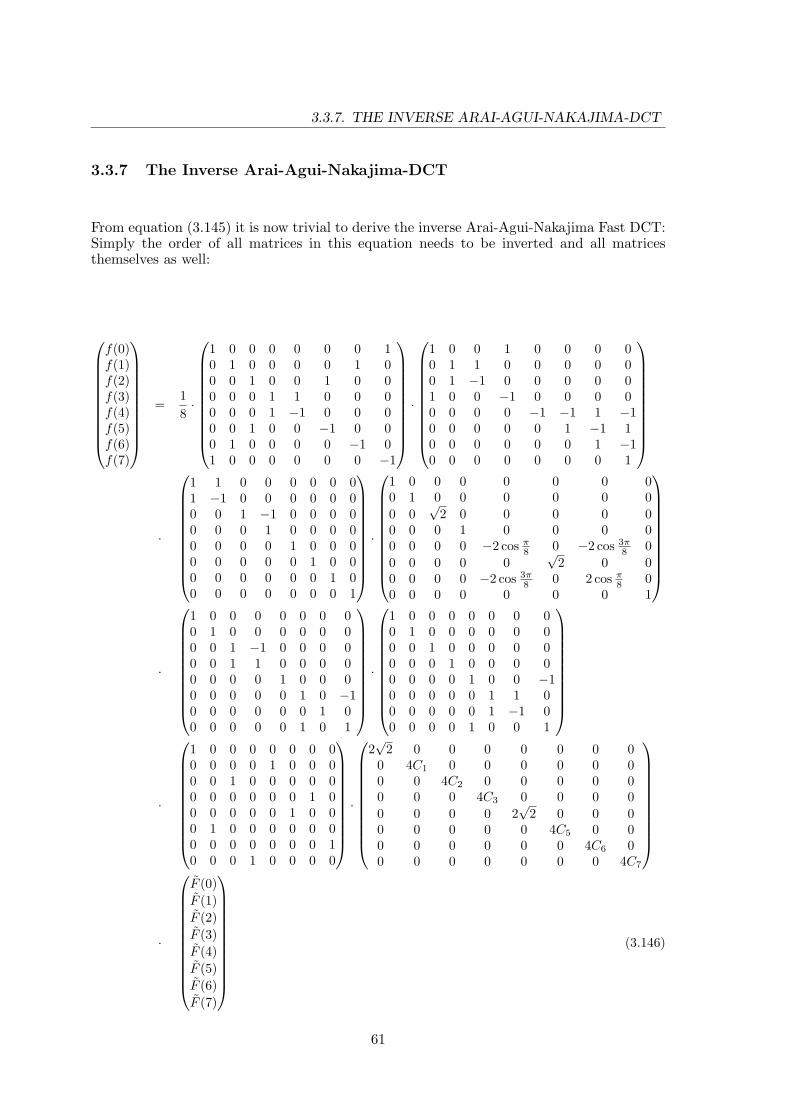
3.3.7. THE INVERSE ARAI-AGUI-NAKAJIMA-DCT
3.3.7 The Inverse Arai-Agui-Nakajima-DCT
From equation (3.145) it is now trivial to derive the inverse Arai-Agui-Nakajima Fast DCT:Simply the order of all matrices in this equation needs to be inverted and all matricesthemselves as well:
f(0)f(1)f(2)f(3)f(4)f(5)f(6)f(7)
=
18·
1 0 0 0 0 0 0 10 1 0 0 0 0 1 00 0 1 0 0 1 0 00 0 0 1 1 0 0 00 0 0 1 −1 0 0 00 0 1 0 0 −1 0 00 1 0 0 0 0 −1 01 0 0 0 0 0 0 −1
·
1 0 0 1 0 0 0 00 1 1 0 0 0 0 00 1 −1 0 0 0 0 01 0 0 −1 0 0 0 00 0 0 0 −1 −1 1 −10 0 0 0 0 1 −1 10 0 0 0 0 0 1 −10 0 0 0 0 0 0 1
·
1 1 0 0 0 0 0 01 −1 0 0 0 0 0 00 0 1 −1 0 0 0 00 0 0 1 0 0 0 00 0 0 0 1 0 0 00 0 0 0 0 1 0 00 0 0 0 0 0 1 00 0 0 0 0 0 0 1
·
1 0 0 0 0 0 0 00 1 0 0 0 0 0 00 0
√2 0 0 0 0 0
0 0 0 1 0 0 0 00 0 0 0 −2 cos π
8 0 −2 cos 3π8 0
0 0 0 0 0√
2 0 00 0 0 0 −2 cos 3π
8 0 2 cos π8 0
0 0 0 0 0 0 0 1
·
1 0 0 0 0 0 0 00 1 0 0 0 0 0 00 0 1 −1 0 0 0 00 0 1 1 0 0 0 00 0 0 0 1 0 0 00 0 0 0 0 1 0 −10 0 0 0 0 0 1 00 0 0 0 0 1 0 1
·
1 0 0 0 0 0 0 00 1 0 0 0 0 0 00 0 1 0 0 0 0 00 0 0 1 0 0 0 00 0 0 0 1 0 0 −10 0 0 0 0 1 1 00 0 0 0 0 1 −1 00 0 0 0 1 0 0 1
·
1 0 0 0 0 0 0 00 0 0 0 1 0 0 00 0 1 0 0 0 0 00 0 0 0 0 0 1 00 0 0 0 0 1 0 00 1 0 0 0 0 0 00 0 0 0 0 0 0 10 0 0 1 0 0 0 0
·
2√
2 0 0 0 0 0 0 00 4C1 0 0 0 0 0 00 0 4C2 0 0 0 0 00 0 0 4C3 0 0 0 00 0 0 0 2
√2 0 0 0
0 0 0 0 0 4C5 0 00 0 0 0 0 0 4C6 00 0 0 0 0 0 0 4C7
·
F (0)F (1)F (2)F (3)F (4)F (5)F (6)F (7)
(3.146)
61

CHAPTER 3. THE DISCRETE COSINE TRANSFORM
Notice that the lower right half of the second matrix in equation (3.146) can be factored asfollows:
−1 −1 1 −10 1 −1 10 0 1 −10 0 0 1
=
−1 −1 0 00 1 0 00 0 1 00 0 0 1
·
1 0 0 00 1 −1 00 0 1 00 0 0 1
·
1 0 0 00 1 0 00 0 1 −10 0 0 1
(3.147)
If we now consider that the lower right half of the fourth matrix in equation (3.146)contains a rotation of rows 4 and 6 of the following matrix which can be written as(
−2 cos π8
−2 cos 3π8
−2 cos 3π8
2 cos π8
)=(−1 1 0
1 0 1
)·
(2 cos π
80 0
0 2(cos π8−cos 3π
8 ) 0
0 0 −2(cos π8+cos 3π
8 )
)·(
1 10 11 0
), we are able
to derive a flowgraph for the inverse Arai-Agui-Nakajima Fast DCT as depicted in figure3.11.
4·C ·F(2)
4·C ·F(6)
4·C ·F(5)
4·C ·F(1)
4·C ·F(7)
4·C ·F(3)
2a1
2a4
2a3
2a2
2a6
8·f(0)
8·f(6)
8·f(1)
8·f(2)
8·f(3)
8·f(4)
8·f(5)
8·f(7)
2· 2·F(4)
2
6
5
1
7
3
2· 2·F(0)~
~
~
~
~
~
~
~
Figure 3.11: Flowgraph for the inverse Arai-Agui-Nakajima Fast DCT
Figure 3.11 uses a new constant besides from the ones in equation (3.144):
a6 = cosπ
8(3.148)
62

3.4. FAST TWO-DIMENSIONAL DCTS
3.4 Fast two-dimensional DCTs
In this section we are going to develop a fast two-dimensional 8-point DCT from the Arai-Agui-Nakajima DCT in section 3.3.6. We will show that the two-dimensional DCT isactually the tensor product of the DCT matrix with itself. Therefore the tensor productand its most important properties will first be covered in more detail.
3.4.1 The tensor product and its properties
In section 3.3.5 we already introduced the tensor product. A good introduction on this topiccan also be found in [13]. The tensor product is a binary matrix operator that provides amechanism for combining two matrices to form one single larger matrix. Let An1,n2 andBm1,m2 be two arbitrary matrices of dimension n1 × n2 and m1 ×m2, respectively:
An1,n2 =
a0,0 a0,1 . . . a0,n2−1
a1,0 a1,1 . . . a1,n2−1...
......
an1−1,0 an1−1,1 . . . an1−1,n2−1
(3.149)
Bm1,m2 =
b0,0 b0,1 . . . b0,m2−1
b1,0 b1,1 . . . b1,m2−1...
......
bm1−1,0 bm1−1,1 . . . bm1−1,m2−1
(3.150)
The tensor product C = A⊗B is defined as the n1m1 × n2m2 matrix given by:
C = An1,n2 ⊗Bm1,m2 =
a0,0 ·B a0,1 ·B . . . a0,n2−1 ·Ba1,0 ·B a1,1 ·B . . . a1,n2−1 ·B
......
...an1−1,0 ·B an1−1,1 ·B . . . an1−1,n2−1 ·B
(3.151)
This means that the tensor product of A and B is formed by replacing an arbitrary elementaij of A with the m1 ×m2 matrix aij ·B.
There are quite a few interesting properties of the tensor product, for instance, it isassociative:
A⊗ (B ⊗ C) = (A⊗B)⊗ C (3.152)
If the involved matrices are of appropriate dimension, the tensor product is also distributiveover matrix multiplication:
(A⊗B) · (C ⊗D) = AC ⊗BD (3.153)
Another property is the inversion property: If A and B are nonsingular matrices, so isC = A⊗B and:
C−1 = (A⊗B)−1 = A−1 ⊗B−1 (3.154)
63

CHAPTER 3. THE DISCRETE COSINE TRANSFORM
This means that if we want to calculate the inverse matrix of a large matrix C that canbe expressed as a tensor product, the inverse can be much more easily calculated from aninversion of the factors A and B.
Another interesting property of the tensor product is the transposition property :
(A⊗B)t = At ⊗Bt (3.155)
The last property to be examined will be needed quite often in the following sections. Itallows us to reverse the order of operators in the tensor product with the help of permutationmatrices: In section 3.3.5 we used the permutation matrix that permuted the rows of avector or a matrix in the following order: 0, 2, 4, 6, 8, 10, 12, 14, 1, 3, 5, 7, 9, 11, 13,15. This matrix is actually called a stride-by-2 matrix. Generally, a stride-by-s matrix
works like this: Let Xn =
( x0x1
...xn
)be an n-point vector and let Pn,s denote the stride-by-
s permutation matrix with n = r · s. For the caculation of Yn = Pn,s · Xn, the first relements of Yn are obtained by starting at element x0 and selecting each sth element of Xn.The next r elements are obtained in the same manner, but this time starting at x1. Thisprocess is repeated s times in total and the vector Yn is built from the following elements:x0, xs, x2s, . . . , x(r−1)s, x1, xs+1, x2s+1, . . . , x(r−1)s+1, . . . , xs−1, x2s−1, . . . , xrs−1. Now let As
and Br be any sqare matrices of order s and r, respectively. Then we can reverse the orderof the tensor product with a stride-by-s and a stride-by-r permutation matrix:
(As ⊗Br) = Pn,s · (Br ⊗As) · Pn,r (3.156)
3.4.2 The two-dimensional DCT as a tensor product
Let K8 be the DCT matrix that is built from the product of all matrices in equation (3.145)such that equation (3.145) can be written as:
F (0)F (1)F (2)F (3)F (4)F (5)F (6)F (7)
= K8 ·
f(0)f(1)f(2)f(3)f(4)f(5)f(6)f(7)
(3.157)
For calculating a two-dimensional n-point DCT, we use an n × n input vector that is builtfrom appending all n rows together. We then apply a one-dimensional DCT individuallyon each group of n points, which corresponds to calculating the row-wise DCT. Then wepermute the result vector such that all n first vector elements of each group are groupedtogether, then all n second vector elements, and so on. On the resulting vector, again to eachgroup of n points, individual n-point DCTs are applied, which corresponds to calculatingthe column-wise DCT. Finally, the elements of the result vector have to be permuted againin the same way as between the first row-wise DCT and the column-wise DCT. For a two-dimensional 8-point DCT this can now be written in the form of a matrix-vector product
64

3.4.2. THE TWO-DIMENSIONAL DCT AS A TENSOR PRODUCT
as follows:
F (0, 0)F (0, 1)
...F (0, 7)F (1, 0)F (1, 1)
...F (1, 7)
...F (7, 0)F (7, 1)
...F (7, 7)
= P64,8 ·
K8 . . . 0
K8 . . ....
K8
K8
K8
K8... . . . K8
0 . . . K8
·P64,8 ·
K8 . . . 0
K8 . . ....
K8
K8
K8
K8... . . . K8
0 . . . K8
·
f(0, 0)f(0, 1)
...f(0, 7)f(1, 0)f(1, 1)
...f(1, 7)
...f(7, 0)f(7, 1)
...f(7, 7)
(3.158)
= P64,8 · (I8 ⊗K8) · P64,8 · (I8 ⊗K8) ·
f(0, 0)f(0, 1)
...f(0, 7)f(1, 0)f(1, 1)
...f(1, 7)
...f(7, 0)f(7, 1)
...f(7, 7)
65

CHAPTER 3. THE DISCRETE COSINE TRANSFORM
Now, since (I8 ⊗K8) = P64,8 · (K8 ⊗ I8) · P64,8 and P64,8 · P64,8 = I8 we can write:
P64,8 · (I8 ⊗K8) · P64,8 · (I8 ⊗K8) = P64,8 · P64,8 · (K8 ⊗ I8) · P64,8 · P64,8 · (I8 ⊗K8) =(K8 ⊗ I8) · (I8 ⊗K8) = (K8 · I8)⊗ (I8 ·K8) = K8 ⊗K8 (3.159)
With equation (3.159) we now get from equation (3.158):
F (0, 0)F (0, 1)
...F (0, 7)F (1, 0)F (1, 1)
...F (1, 7)
...F (7, 0)F (7, 1)
...F (7, 7)
= (K8 ⊗K8)
f(0, 0)f(0, 1)
...f(0, 7)f(1, 0)f(1, 1)
...f(1, 7)
...f(7, 0)f(7, 1)
...f(7, 7)
(3.160)
This shows, that the matrix for the two-dimensional DCT can be built from applying thetensor product of the one-dimensional DCT to itself.
3.4.3 Feig’s fast two-dimensional DCT
This section will deal with a true two-dimensional approach to the calculation of the 2D 8-point DCT. It was published by E. Feig in 1990 ([8]). A good introduction into this algorithmcan also be found in [22] (1993) and in [9] (1992). Feig’s algorithm takes the Arai-Agui-Nakajima DCT as the basis and achieves a computational complexity of 54 multiplications,6 shift operations and 462 additions, whereas an Arai-Agui-Nakajima DCT in row-columnscheme would require 16× 5 = 80 multiplications and 16× 29 = 464 additions.
From section 3.4.2 we know, that the two-dimensional DCT can be expressed as thetensor product of the one-dimensional DCT with itself (see equations (3.159) and (3.160)).From equation (3.145) we also know, that the Arai-Agui-Nakajima DCT can be expressedas a product of matrices with an 8-point input vector as follows:
F (0)F (1)F (2)F (3)F (4)F (5)F (6)F (7)
= K8 ·
f(0)f(1)f(2)f(3)f(4)f(5)f(6)f(7)
= DF · PF ·BF ·MF ·AF ·
f(0)f(1)f(2)f(3)f(4)f(5)f(6)f(7)
(3.161)
66

3.4.3. FEIG’S FAST TWO-DIMENSIONAL DCT
The matrices DF , PF , BF , MF and AF are as follows (compare with equation(3.145)):
DF =
12√
20 0 0 0 0 0 0
0 14C1
0 0 0 0 0 00 0 1
4C20 0 0 0 0
0 0 0 14C3
0 0 0 00 0 0 0 1
2√
20 0 0
0 0 0 0 0 14C5
0 00 0 0 0 0 0 1
4C60
0 0 0 0 0 0 0 14C7
(3.162)
PF =
1 0 0 0 0 0 0 00 0 0 0 0 1 0 00 0 1 0 0 0 0 00 0 0 0 0 0 0 10 1 0 0 0 0 0 00 0 0 0 1 0 0 00 0 0 1 0 0 0 00 0 0 0 0 0 1 0
(3.163)
BF =
1 0 0 0 0 0 0 00 1 0 0 0 0 0 00 0 1 0 0 0 0 00 0 0 1 0 0 0 00 0 0 0 1 0 0 10 0 0 0 0 1 1 00 0 0 0 0 1 −1 00 0 0 0 −1 0 0 1
·
1 0 0 0 0 0 0 00 1 0 0 0 0 0 00 0 1 1 0 0 0 00 0 −1 1 0 0 0 00 0 0 0 1 0 0 00 0 0 0 0 1 0 10 0 0 0 0 0 1 00 0 0 0 0 −1 0 1
(3.164)
MF =
1 0 0 0 0 0 0 00 1 0 0 0 0 0 00 0 1√
20 0 0 0 0
0 0 0 1 0 0 0 00 0 0 0 − cos π
8 0 − cos 3π8 0
0 0 0 0 0 1√2
0 00 0 0 0 − cos 3π
8 0 cos π8 0
0 0 0 0 0 0 0 1
(3.165)
67

CHAPTER 3. THE DISCRETE COSINE TRANSFORM
f(0)
f(1)
f(2)
f(3)
f(4)
f(5)
f(6)
f(7)
Figure 3.12: Flowgraph for matrix AF
AF =
1 1 0 0 0 0 0 01 −1 0 0 0 0 0 00 0 1 1 0 0 0 00 0 0 1 0 0 0 00 0 0 0 1 0 0 00 0 0 0 0 1 0 00 0 0 0 0 0 1 00 0 0 0 0 0 0 1
·
1 0 0 1 0 0 0 00 1 1 0 0 0 0 00 1 −1 0 0 0 0 01 0 0 −1 0 0 0 00 0 0 0 −1 −1 0 00 0 0 0 0 1 1 00 0 0 0 0 0 1 10 0 0 0 0 0 0 1
·
1 0 0 0 0 0 0 10 1 0 0 0 0 1 00 0 1 0 0 1 0 00 0 0 1 1 0 0 00 0 0 1 −1 0 0 00 0 1 0 0 −1 0 00 1 0 0 0 0 −1 01 0 0 0 0 0 0 −1
(3.166)
Figures 3.12, 3.14 and 3.13 show the flowgraphs of matrices AF , BF and MF , respec-tively. For figure 3.13, the values of a1, a2, a3, a4 and a5 are the ones from equation(3.144).
The tensor product K8 ⊗K8 can be now written as:
K8 ⊗K8 = (DF · PF ·BF ·MF ·AF )⊗ (DF · PF ·BF ·MF ·AF ) (3.167)
68

3.4.3. FEIG’S FAST TWO-DIMENSIONAL DCT
a1
a2
a3
a4
a5
Figure 3.13: Flowgraph for matrix MF
m F(0)
m F(7)
m F(4)
m F(2)
m F(6)
m F(5)
m F(1)
m F(3)
0
4
2
6
5
1
7
3
~
~
~
~
~
~
~
~
Figure 3.14: Flowgraph for matrix BF
69

CHAPTER 3. THE DISCRETE COSINE TRANSFORM
From the distributive property of the tensor product we get:
K8 ⊗K8 = (DF ⊗DF ) · ((PF ·BF ·MF ·AF )⊗ (PF ·BF ·MF ·AF )) (3.168)
With the shortcut K ′8 = PF ·BF ·MF ·AF we can now write:
K8 ⊗K8 = (DF ⊗DF ) · (K ′8 ⊗K ′
8) (3.169)
The matrix (DF ⊗DF ) is a diagonal matrix of dimension 64× 64, containing the 64 scalingfactors that can be absorbed into the quantization values. For practical reasons, in thefollowing we will rather deal with (K ′
8 ⊗ K ′8) than (K8 ⊗ K8), keeping in mind, that the
result vector of (K ′8 ⊗K ′
8) needs to be scaled by (DF ⊗DF ).Again using the distributive property of tensor products, we can express (K ′
8 ⊗K ′8) as
follows:
(K ′8 ⊗K ′
8) = (PF ⊗ PF ) · (BF ⊗BF ) · (MF ⊗MF ) · (AF ⊗AF ) (3.170)
The matrix (PF ⊗ PF ) in equation (3.170) is simply a 64 × 64 permutation matrix thatreorders the output to natural order, but does not contribute to computational complexity.For the other factors in equation (3.170) we can now choose whether we want to apply a row-column scheme, or whether we want to calculate the tensor product to form a 64×64 matrix.Feig’s approach was to use a row-column scheme for the tensor products (BF ⊗ BF ) and(AF ⊗AF ), which contain merely additions, but to calculate the tensor product (MF ⊗MF ),which contains all the multiplications.
The tensor product (AF ⊗AF ) can be written as follows:
(AF ⊗AF ) = (I8 ·AF )⊗ (AF · I8) = (I8 ⊗AF ) · (AF ⊗ I8) (3.171)
Using equation (3.156), this can be written as follows:
(AF ⊗AF ) = (I8 ⊗AF ) · P64,8 · (I8 ⊗AF ) · P64,8 (3.172)
Matrix P64,8 simply permutes the 64 elements of the input vector, and (I8 ⊗ AF ) can beexpanded to the following 64× 64 matrix:
(I8 ⊗AF ) =
AF 0 0 0 0 0 0 00 AF 0 0 0 0 0 00 0 AF 0 0 0 0 00 0 0 AF 0 0 0 00 0 0 0 AF 0 0 00 0 0 0 0 AF 0 00 0 0 0 0 0 AF 00 0 0 0 0 0 0 AF
(3.173)
Equations (3.172) and (3.173) are illustrated in the form of a flowgraph in figure 3.15.Note that this flowgraph uses a hollow square at line ends to represent an 8-element vectorinput and output of an 8×8 matrix. The boxes labeled AF and P64,8 represent the respectivematrices. Also, the initial permutation with the stride-by-8 permutation matrix is alreadyrepresented by the choice of the input vectors to the left row of the matrices labeled withAF .
70

3.4.3. FEIG’S FAST TWO-DIMENSIONAL DCT
f(0,0)f(0,1)
f(0,7)
····
f(1,0)f(1,1)
f(1,7)
····
f(2,0)f(2,1)
f(2,7)
····
f(3,0)f(3,1)
f(3,7)
····
f(4,0)f(4,1)
f(4,7)
····
f(5,0)f(5,1)
f(5,7)
····
f(6,0)f(6,1)
f(6,7)
····
f(7,0)f(7,1)
f(7,7)
····
P64,8
A F
A F
A F
A F
A F
A F
A F
A F A F
A F
A F
A F
A F
A F
A F
A F
Figure 3.15: Flowgraph for matrix AF ⊗AF
71

CHAPTER 3. THE DISCRETE COSINE TRANSFORM
Similar to (AF ⊗AF ) in equation (3.172), (BF ⊗BF ) can be expressed as follows:
(BF⊗BF ) = BF ·I8⊗I8·BF = (BF⊗I8)·(I8⊗BF ) = P64,8·(I8⊗BF )·P64,8·(I8⊗BF ) (3.174)
Matrix (I8 ⊗BF ) can be expanded to the following 64× 64 matrix:
(I8 ⊗BF ) =
BF 0 0 0 0 0 0 00 BF 0 0 0 0 0 00 0 BF 0 0 0 0 00 0 0 BF 0 0 0 00 0 0 0 BF 0 0 00 0 0 0 0 BF 0 00 0 0 0 0 0 BF 00 0 0 0 0 0 0 BF
(3.175)
Equation (3.175) is illustrated in the form of a flowgraph in figure 3.16. Like the initialpermutation in figure 3.15, the final permutation with the stride-by-8 permutation matrixis already represented by the choice of the output vectors of the right row of the matriceslabeled with BF . The output vectors in figure 3.16 are the values of the DCT with thescaling factors from (DF ⊗DF ) omitted and without the final permutation with (PF ⊗PF ),therefore they are labeled F ′(u, v) to avoid confusion with the output F (n, m) of the DCT.Again, this flowgraph uses a hollow square at line ends to represent an 8-element vectorinput and output of an 8 × 8 matrix and the boxes labeled BF and P64,8 represent therespective matrices.
The last missing tensor product in equation (3.170), MF ⊗ MF , can be written in theform of a 64× 64 matrix as follows:
(MF ⊗MF ) =
MF 0 0 0 0 0 0 00 MF 0 0 0 0 0 00 0 C4 ·MF 0 0 0 0 00 0 0 MF 0 0 0 00 0 0 0 −C2 ·MF 0 −C6 ·MF 00 0 0 0 0 C4 ·MF 0 00 0 0 0 −C6 ·MF 0 C2 ·MF 00 0 0 0 0 0 0 MF
(3.176)
Rows 0, 1, 3 and 7 represent 4 matrices M1 = MF , each operating on a sequence of 8elements of the input vector, therefore contributing 4 × 3 = 12 additions and 4 × 5 = 20multiplications to the overall complexity of this algorithm. See figure 3.13 for a flowgraphof M1 = MF .
Rows 2 and 5 each represent a variant of matrix MF that is scaled by C4. Each of thesetwo matrices M2 = C4 · MF is operating on a sequence of 8 input elements of the inputvector. While M2 requires 9 multiplications, 2 of them are actually multiplications withC4 · C4 = 1
2 , which can be easily performed by a right shift operation. The 8 × 8 matrix
72

3.4.3. FEIG’S FAST TWO-DIMENSIONAL DCT
F'(0,0)F'(0,1)
F'(0,7)
····
F'(1,0)F'(1,1)
F'(1,7)
····
F'(2,0)F'(2,1)
F'(2,7)
····
F'(3,0)F'(3,1)
F'(3,7)
····
F'(4,0)F'(4,1)
F'(4,7)
····
F'(5,0)F'(5,1)
F'(5,7)
····
F'(6,0)F'(6,1)
F'(6,7)
····
F'(7,0)F'(7,1)
F'(7,7)
····
P64,8
~~
~
~~
~
~~
~
~~
~
~~
~
~~
~
~~
~
~~
~
B F
B F
B F
B F
B F B F
B F
B F
B F
B F
B F B F
B FB F
B F B F
Figure 3.16: Flowgraph for matrix BF ⊗BF
73

CHAPTER 3. THE DISCRETE COSINE TRANSFORM
12
a5
a6
a2
a1
a1
a1
a1
12
12
Figure 3.17: Flowgraph for matrix M2
M2 = C4 ·MF can therefore be written as follows:
M2 = C4 ·MF =
C4 0 0 0 0 0 0 00 C4 0 0 0 0 0 00 0 1
2 0 0 0 0 00 0 0 C4 0 0 0 00 0 0 0 −C2 · C4 0 −C6 · C4 00 0 0 0 0 1
2 0 00 0 0 0 −C6 · C4 0 C2 · C4 00 0 0 0 0 0 0 C4
(3.177)
Figure 3.17 shows the flowgraph of M2 from which we can see, that the two rows in equation(3.176) with M2 = C4 ·MF contribute 2× 7 = 14 multiplications, 2× 3 = 6 additions and2 × 2 = 4 shift operations to the overall complexity of the Feig 2D-DCT. The constantsused in figure 3.17 are the ones from equations (3.144) and (3.148).
The remaining rows and columns in equation (3.176) can be represented by the tensor
74

3.4.3. FEIG’S FAST TWO-DIMENSIONAL DCT
a2
a4
a5
Figure 3.18: Flowgraph for matrix N1
product M3 =(−C2 −C6−C6 C2
)⊗MF = N ⊗MF with
N =(−C2 −C6
−C6 C2
)=(
1 1 01 0 1
)·
− cos 3π8 0 0
0 (cos 3π8 − cos π
8 ) 00 0
(cos π
8 + cos 3π8
)·1 1
1 00 1
(3.178)
With equation (3.156) the tensor product M3 = N ⊗MF can be written as:
M3 = N ⊗MF = P16,2 · (MF ⊗ N) · P16,8 (3.179)
The 16× 16 matrix MF ⊗ N is defined as:
(MF ⊗ N) =
N 0 0 0 0 0 0 00 N 0 0 0 0 0 00 0 C4 · N 0 0 0 0 00 0 0 N 0 0 0 00 0 0 0 −C2 · N 0 −C6 · N 00 0 0 0 0 C4 · N 0 00 0 0 0 −C6 · N 0 C2 · N 00 0 0 0 0 0 0 N
(3.180)
This means, that the first, second, fourth and eighth pair of input vector elements of MF⊗Nare matrix-multiplied by N1 = N and that the third and fifth pair of input vector elementsof MF ⊗ N are matrix-multiplied by a scaled variant of N , N2 = C4 · N . These 6 matrixmultiplications require each 3 multiplications and 3 additions. Figures 3.18 and 3.19 showthe flowgraphs of N1 and N2, respectively. The constants used in figure 3.19 are the onesfrom equations (3.144) and (3.148).
The remaining rows in equation (3.180) can be expressed as the tensor product
75

CHAPTER 3. THE DISCRETE COSINE TRANSFORM
a5
a 6
a212
Figure 3.19: Flowgraph for matrix N2
C 2
4
C 2
4
12
12
Figure 3.20: Flowgraph for matrix N3 = N ⊗ N
N3 = N ⊗ N and can be written in matrix form and factorized as follows:
N3 = (N ⊗ N) =12·
(1 + C4) C4 C4 (1− C4)
C4 −(1 + C4) (1− C4) −C4
C4 (1− C4) −(1 + C4) −C4
(1− C4) −C4 −C4 (1 + C4)
(3.181)
=
1 0 0 10 1 −1 00 1 1 0−1 0 0 1
·
1 1 0 01 −1 0 00 0 1 00 0 0 1
·
C42 0 0 00 C4
2 0 00 0 1
2 00 0 0 1
2
·
1 0 0 −10 1 1 00 1 −1 01 0 0 1
Thus, N3 = N ⊗ N can be calculated with 10 additions, 2 multiplications and 2 shiftoperations. Figure 3.20 shows the flowgraph of N3 = N ⊗ N with C4 defined accordingto equation (3.38). If we combine the flowgraphs in figures 3.18, 3.19, and 3.20 for thematrices N1, N2 and N3, we get the flowgraph for matrix M3 = N ⊗ MF in figure 3.21.The constants used in figure 3.21 are the ones from equations (3.38), (3.144) and (3.148).
Now that we have all individual flowgraphs for AF ⊗AF , BF ⊗BF , M1, M2 and M3, wecan finally derive a flowgraph for the calculation of K ′
8 ⊗K ′8 without the final permutation
76

3.4.3. FEIG’S FAST TWO-DIMENSIONAL DCT
C 2
4
C 2
4
12
12
a 2
a 4
a 5
a 2
a 4
a 5
a 2
a 4
a 5
a 2
a 4
a 5
a5
a 6
a5
a 6
P16,8 P16,2M N⊗F
a 212 ·
a 212 ·
~
Figure 3.21: Flowgraph for matrix M3 = N ⊗MF
77

CHAPTER 3. THE DISCRETE COSINE TRANSFORM
Stage Multiplications Additions Shifts
BF ⊗BF 0 16× 18 0AF ⊗AF 0 16× 8 0MF ⊗MF :
Rows 1, 2, 4, 8 (M1) 4× 5 4× 3 0Rows 3, 6 (M2) 2× 7 2× 3 2× 2Rows 5, 7 (MF ⊗ N):
Rows 1, 2, 4, 8 (N1) 4× 3 4× 3 0Rows 3, 6 (N2) 2× 3 2× 3 0Rows 5, 7 (N3) 2 10 2
Totals: 54 462 6
Table 3.1: Computational complexity of Feig’s 2D DCT
by PF ⊗PF in figure 3.22 and sum up the operations of the different stages in Feig’s scaled2D DCT in table 3.1.
78

3.4.3. FEIG’S FAST TWO-DIMENSIONAL DCTf(
0,0
)f(
0,1
)
f(0
,7)
· · ··
f(1
,0)
f(1
,1)
f(1
,7)
· · ··
f(2
,0)
f(2
,1)
f(2
,7)
· · ··
f(3
,0)
f(3
,1)
f(3
,7)
· · ··
f(4
,0)
f(4
,1)
f(4
,7)
· · ··
f(5
,0)
f(5
,1)
f(5
,7)
· · ··
f(6
,0)
f(6
,1)
f(6
,7)
· · ··
f(7
,0)
f(7
,1)
f(7
,7)
· · ··
P 64
,8
F'(0
,0)
F'(0
,1)
F'(0
,7)
· · ··
F'(1
,0)
F'(1
,1)
F'(1
,7)
· · ··
F'(2
,0)
F'(2
,1)
F'(2
,7)
· · ··
F'(3
,0)
F'(3
,1)
F'(3
,7)
· · ··
F'(4
,0)
F'(4
,1)
F'(4
,7)
· · ··
F'(5
,0)
F'(5
,1)
F'(5
,7)
· · ··
F'(6
,0)
F'(6
,1)
F'(6
,7)
· · ··
F'(7
,0)
F'(7
,1)
F'(7
,7)
· · ··
P 64
,8
~ ~ ~ ~ ~ ~ ~ ~ ~ ~ ~ ~ ~ ~ ~ ~ ~ ~ ~ ~ ~ ~ ~ ~
1M
1M
2M
1M
2M
3M
1M
BF
BF
BF
BF
BF
BF
BF
BF
BF
BF
BF
BF
BF
BF
BF
BF
AF
AF
AF
AF
AF
AF
AFAF
AF
AF
AF
AF
AF
AF
AF
AF
Fig
ure
3.22
:Flo
wgr
aph
ofK
′ 8⊗
K′ 8
wit
hout
the
final
perm
utat
ion
by(P
⊗P
)
79

CHAPTER 3. THE DISCRETE COSINE TRANSFORM
3.4.4 Feig’s fast two-dimensional inverse DCT
This section will show in a similar manner to section 3.4.3 how the inverse Arai-Agui-Nakajima DCT can be extended to a true two-dimensional DCT.
From equation (3.146) we can derive the following for the inverse Arai-Agui-NakajimaDCT:
f(0)f(1)f(2)f(3)f(4)f(5)f(6)f(7)
= K8
−1 ·
F (0)F (1)F (2)F (3)F (4)F (5)F (6)F (7)
= AI ·MI ·BI · PI ·DI ·
F (0)F (1)F (2)F (3)F (4)F (5)F (6)F (7)
(3.182)
The matrices AI , MI , BI , PI and DI are as follows (compare with equation(3.146)):
AI =
1 0 0 0 0 0 0 10 1 0 0 0 0 1 00 0 1 0 0 1 0 00 0 0 1 1 0 0 00 0 0 1 −1 0 0 00 0 1 0 0 −1 0 00 1 0 0 0 0 −1 01 0 0 0 0 0 0 −1
·
1 0 0 1 0 0 0 00 1 1 0 0 0 0 00 1 −1 0 0 0 0 01 0 0 −1 0 0 0 00 0 0 0 −1 −1 1 −10 0 0 0 0 1 −1 10 0 0 0 0 0 1 −10 0 0 0 0 0 0 1
·
1 1 0 0 0 0 0 01 −1 0 0 0 0 0 00 0 1 −1 0 0 0 00 0 0 1 0 0 0 00 0 0 0 1 0 0 00 0 0 0 0 1 0 00 0 0 0 0 0 1 00 0 0 0 0 0 0 1
(3.183)
MI =
1 0 0 0 0 0 0 00 1 0 0 0 0 0 00 0
√2 0 0 0 0 0
0 0 0 1 0 0 0 00 0 0 0 −2 cos π
8 0 −2 cos 3π8 0
0 0 0 0 0√
2 0 00 0 0 0 −2 cos 3π
8 0 2 cos π8 0
0 0 0 0 0 0 0 1
(3.184)
80

3.4.4. FEIG’S FAST TWO-DIMENSIONAL INVERSE DCT
BI =
1 0 0 0 0 0 0 00 1 0 0 0 0 0 00 0 1 −1 0 0 0 00 0 1 1 0 0 0 00 0 0 0 1 0 0 00 0 0 0 0 1 0 −10 0 0 0 0 0 1 00 0 0 0 0 1 0 1
·
1 0 0 0 0 0 0 00 1 0 0 0 0 0 00 0 1 0 0 0 0 00 0 0 1 0 0 0 00 0 0 0 1 0 0 −10 0 0 0 0 1 1 00 0 0 0 0 1 −1 00 0 0 0 1 0 0 1
(3.185)
PI =
1 0 0 0 0 0 0 00 0 0 0 1 0 0 00 0 1 0 0 0 0 00 0 0 0 0 0 1 00 0 0 0 0 1 0 00 1 0 0 0 0 0 00 0 0 0 0 0 0 10 0 0 1 0 0 0 0
(3.186)
DI =
12√
20 0 0 0 0 0 0
0 C12 0 0 0 0 0 0
0 0 C22 0 0 0 0 0
0 0 0 C32 0 0 0 0
0 0 0 0 12√
20 0 0
0 0 0 0 0 C52 0 0
0 0 0 0 0 0 C62 0
0 0 0 0 0 0 0 C72
(3.187)
Figures 3.23, 3.24 and 3.25 show the flowgraphs of matrices AI , BI and MI , respectively.For figure 3.25, the values of a1, a2, a3, a4 and a5 are the ones from equation (3.144). Withthe help of the inversion property (see equation (3.154)) of the tensor product, (K8 ⊗K8)
−1
can now be written as:
(K8 ⊗K8)−1 = K−1
8 ⊗K−18 = (AI ·MI ·BI · PI ·DI)⊗ (AI ·MI ·BI · PI ·DI) (3.188)
From the distributive property of the tensor product we get:
(K8 ⊗K8)−1 = ((AI ·MI ·BI · PI)⊗ (AI ·MI ·BI · PI)) · (DI ⊗DI) (3.189)
With the shortcut K ′8−1 = AI ·MI ·BI · PI we can now write:
(K8 ⊗K8)−1 = (K ′
8−1 ⊗K ′
8−1) · (DI ⊗DI) = (K ′
8 ⊗K ′8)−1 · (DI ⊗DI) (3.190)
The matrix (DI ⊗DI) is a diagonal matrix of dimension 64× 64, containing the 64 scalingfactors that can be absorbed into the quantization values. Again, for practical reasons, inthe following we will rather deal with (K ′
8 ⊗K ′8)−1 than (K8 ⊗K8)
−1, keeping in mind,that the input vector of (K ′
8 ⊗K ′8)−1 needs to be scaled by (DI ⊗DI).
81

CHAPTER 3. THE DISCRETE COSINE TRANSFORM
f(0)
f(6)
f(1)
f(2)
f(3)
f(4)
f(5)
f(7)
Figure 3.23: Flowgraph for matrix AI
½·C ·F(2)
½·C ·F(6)
½·C ·F(5)
½·C ·F(1)
½·C ·F(7)
½·C ·F(3)
¼· 2·F(4)
2
6
5
1
7
3
¼· 2·F(0)~
~
~
~
~
~
~
~
Figure 3.24: Flowgraph for matrix BI
82
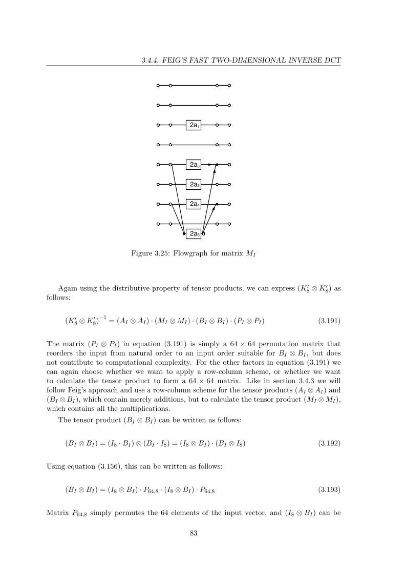
3.4.4. FEIG’S FAST TWO-DIMENSIONAL INVERSE DCT
2a1
2a2
2a3
2a4
2a5
Figure 3.25: Flowgraph for matrix MI
Again using the distributive property of tensor products, we can express (K ′8 ⊗K ′
8) asfollows:
(K ′8 ⊗K ′
8)−1 = (AI ⊗AI) · (MI ⊗MI) · (BI ⊗BI) · (PI ⊗ PI) (3.191)
The matrix (PI ⊗ PI) in equation (3.191) is simply a 64 × 64 permutation matrix thatreorders the input from natural order to an input order suitable for BI ⊗ BI , but doesnot contribute to computational complexity. For the other factors in equation (3.191) wecan again choose whether we want to apply a row-column scheme, or whether we wantto calculate the tensor product to form a 64 × 64 matrix. Like in section 3.4.3 we willfollow Feig’s approach and use a row-column scheme for the tensor products (AI ⊗AI) and(BI ⊗BI), which contain merely additions, but to calculate the tensor product (MI ⊗MI),which contains all the multiplications.
The tensor product (BI ⊗BI) can be written as follows:
(BI ⊗BI) = (I8 ·BI)⊗ (BI · I8) = (I8 ⊗BI) · (BI ⊗ I8) (3.192)
Using equation (3.156), this can be written as follows:
(BI ⊗BI) = (I8 ⊗BI) · P64,8 · (I8 ⊗BI) · P64,8 (3.193)
Matrix P64,8 simply permutes the 64 elements of the input vector, and (I8 ⊗ BI) can be
83

CHAPTER 3. THE DISCRETE COSINE TRANSFORM
expanded to the following 64× 64 matrix:
(I8 ⊗BI) =
BI 0 0 0 0 0 0 00 BI 0 0 0 0 0 00 0 BI 0 0 0 0 00 0 0 BI 0 0 0 00 0 0 0 BI 0 0 00 0 0 0 0 BI 0 00 0 0 0 0 0 BI 00 0 0 0 0 0 0 BI
(3.194)
Equations (3.193) and (3.194) are illustrated in the form of a flowgraph in figure 3.26.Again, this flowgraph uses a hollow square at line ends to represent an 8-element vectorinput and output of an 8×8 matrix. The boxes labeled BI and P64,8 represent the respectivematrices. Also, the initial permutation with the stride-by-8 permutation matrix is alreadyrepresented by the choice of the input vectors to the left row of the matrices labeled withBI . The input vectors in figure 3.26 are the values of the DCT coefficients but with thescaling factors from (DI ⊗DI) and the permutation from (PI ⊗PI) omitted, therefore theyare labeled F ′(u, v) to avoid confusion with the coefficients F (u, v) of the DCT.
Similar to (BI ⊗BI) in equation (3.193), (AI ⊗AI) can be expressed as follows:
(AI⊗AI) = AI ·I8⊗I8 ·AI = (AI⊗I8)·(I8⊗AI) = P64,8 ·(I8⊗AI)·P64,8 ·(I8⊗AI) (3.195)
Matrix (I8 ⊗AI) can be expanded to the following 64× 64 matrix:
(I8 ⊗AI) =
AI 0 0 0 0 0 0 00 AI 0 0 0 0 0 00 0 AI 0 0 0 0 00 0 0 AI 0 0 0 00 0 0 0 AI 0 0 00 0 0 0 0 AI 0 00 0 0 0 0 0 AI 00 0 0 0 0 0 0 AI
(3.196)
Equation (3.196) is illustrated in the form of a flowgraph in figure 3.27. Like the initialpermutation in figure 3.26, the final permutation with the stride-by-8 permutation matrixis already represented by the choice of the output vectors of the right row of the matriceslabeled with AI . Again, this flowgraph uses a hollow square at line ends to represent an8-element vector input and output of an 8 × 8 matrix and the boxes labeled AI and P64,8
represent the respective matrices.The last missing tensor product in equation (3.191), MI ⊗ MI , can be written in the
form of a 64× 64 matrix as follows:
(MI⊗MI) =
MI 0 0 0 0 0 0 00 MI 0 0 0 0 0 00 0
√2 ·MI 0 0 0 0 0
0 0 0 MI 0 0 0 00 0 0 0 −2C2 ·MI 0 −2C6 ·MI 00 0 0 0 0
√2 ·MI 0 0
0 0 0 0 −2C6 ·MI 0 2C2 ·MI 00 0 0 0 0 0 0 MI
(3.197)
84
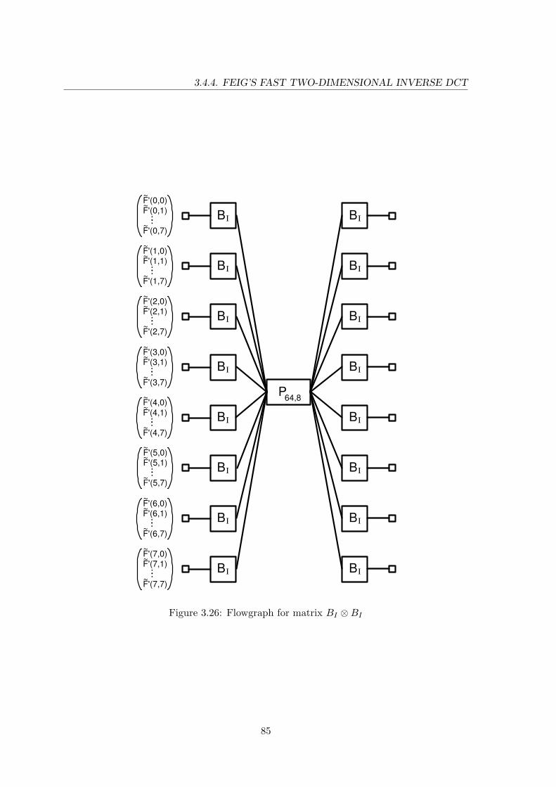
3.4.4. FEIG’S FAST TWO-DIMENSIONAL INVERSE DCT
P64,8
BI
BI
BI
BI
BI
BI
BI
BI
BI
BI
BI
BI
BI
BI
BI
BI
F'(0,0)F'(0,1)
F'(0,7)
····
F'(1,0)F'(1,1)
F'(1,7)
····
F'(2,0)F'(2,1)
F'(2,7)
····
F'(3,0)F'(3,1)
F'(3,7)
····
F'(4,0)F'(4,1)
F'(4,7)
····
F'(5,0)F'(5,1)
F'(5,7)
····
F'(6,0)F'(6,1)
F'(6,7)
····
F'(7,0)F'(7,1)
F'(7,7)
····
~~
~
~~
~
~~
~
~~
~
~~
~
~~
~
~~
~
~~
~
Figure 3.26: Flowgraph for matrix BI ⊗BI
85
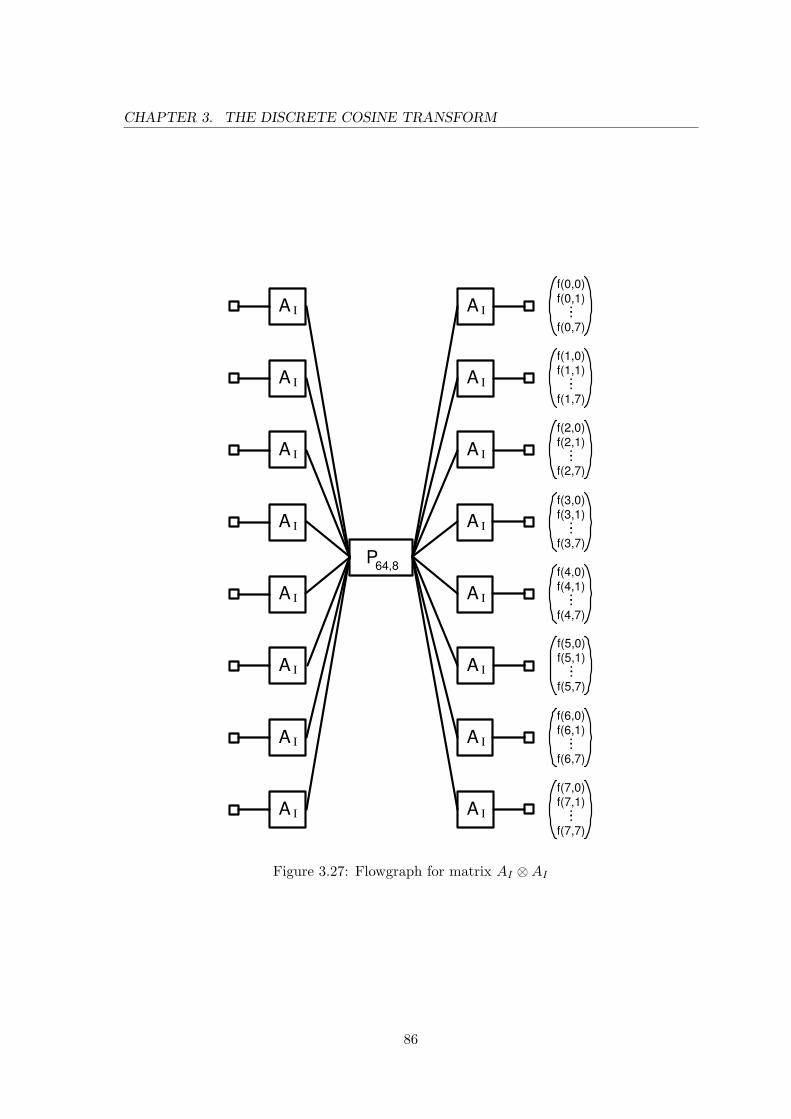
CHAPTER 3. THE DISCRETE COSINE TRANSFORM
P64,8
A I
A I
A I
A I
A I
A I
A I
A I
A I
A I
A I
A I
A I
A I
A I
A I
f(0,0)f(0,1)
f(0,7)
····
f(1,0)f(1,1)
f(1,7)
····
f(2,0)f(2,1)
f(2,7)
····
f(3,0)f(3,1)
f(3,7)
····
f(4,0)f(4,1)
f(4,7)
····
f(5,0)f(5,1)
f(5,7)
····
f(6,0)f(6,1)
f(6,7)
····
f(7,0)f(7,1)
f(7,7)
····
Figure 3.27: Flowgraph for matrix AI ⊗AI
86

3.4.4. FEIG’S FAST TWO-DIMENSIONAL INVERSE DCT
Rows 0, 1, 3 and 7 represent 4 matrices M1 = MI , each operating on a sequence of 8elements of the input vector, therefore contributing 4 × 3 = 12 additions and 4 × 5 = 20multiplications to the overall complexity of this algorithm. See figure 3.25 for a flowgraphof M1 = MI .
Rows 2 and 5 each represent a variant of matrix MI that is scaled by√
2. Each of thesetwo matrices M2 =
√2 · MI is operating on a sequence of 8 input elements of the input
vector. While M2 requires 9 multiplications, 2 of them are actually multiplications with√2 ·
√2 = 2, which can be easily performed by a left shift operation. The 8 × 8 matrix
M2 =√
2 ·MI can be written as follows:
M2 =√
2 ·MI =
√2 0 0 0 0 0 0 0
0√
2 0 0 0 0 0 00 0 2 0 0 0 0 00 0 0
√2 0 0 0 0
0 0 0 0 −2√
2 · C2 0 −2√
2 · C6 00 0 0 0 0 2 0 00 0 0 0 −2
√2 · C6 0 2
√2 · C2 0
0 0 0 0 0 0 0√
2
(3.198)
Figure 3.28 shows the flowgraph of M2 from which we can see, that the two rows in equation(3.197) with M2 =
√2 ·MI contribute 2× 7 = 14 multiplications, 2× 3 = 6 additions and
2 × 2 = 4 shift operations to the overall complexity of the inverse Feig 2D-DCT. Theconstants used in figure 3.28 are the ones from equations (3.144) and (3.148).
The remaining rows and columns in equation (3.197) can be represented by the tensorproduct M3 = 2 ·
(−C2 −C6−C6 C2
)⊗ MI = 2 · N ⊗ MI with N as defined in equation (3.178).
The factor 2 can be absorbed into the diagonal matrix in the factorization of N , so 2N canbe written as:
2N = 2 ·(−C2 −C6
−C6 C2
)(3.199)
=(
1 1 01 0 1
)·
−2 · cos 3π8 0 0
0 2 · (cos 3π8 − cos π
8 ) 00 0 2 ·
(cos π
8 + cos 3π8
) ·
1 11 00 1
With equation (3.156) the tensor product M3 = 2N ⊗MI can be written as:
M3 = 2N ⊗MI = P16,2 · (MI ⊗ 2N) · P16,8 (3.200)
The 16× 16 matrix MI ⊗ 2N is defined as:
(MI⊗2N) =
2N 0 0 0 0 0 0 00 2N 0 0 0 0 0 00 0 2
√2 · N 0 0 0 0 0
0 0 0 2N 0 0 0 00 0 0 0 −4C2 · N 0 −4C6 · N 00 0 0 0 0 2
√2 · N 0 0
0 0 0 0 −4C6 · N 0 4C2 · N 00 0 0 0 0 0 0 2N
(3.201)
87
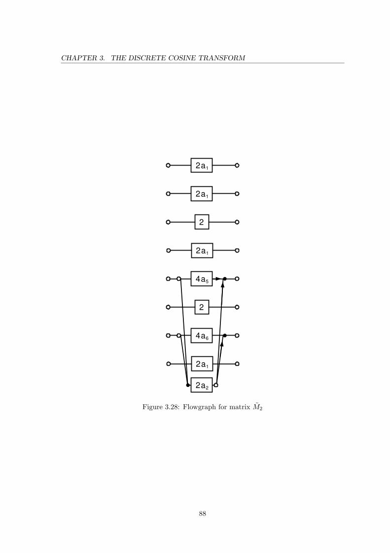
CHAPTER 3. THE DISCRETE COSINE TRANSFORM
2a1
2
2
2a1
2a1
2a1
2a2
4a6
4a5
Figure 3.28: Flowgraph for matrix M2
88

3.4.4. FEIG’S FAST TWO-DIMENSIONAL INVERSE DCT
2·a2
4
5
2·a
2·a
Figure 3.29: Flowgraph for matrix N1
4a5
6
2
4a
2a
Figure 3.30: Flowgraph for matrix N2
This means, that the first, second, fourth and eighth pair of input vector elements of MI⊗2Nare matrix-multiplied by N1 = 2N and that the third and fifth pair of input vector elementsof M ⊗ 2N are matrix-multiplied by a scaled variant of N , N2 = 2
√2 · N . These 6 matrix
multiplications require each 3 multiplications and 3 additions. Figures 3.29 and 3.30 showthe flowgraphs of N1 and N2, respectively. The constants used in figures 3.29 and 3.30 arethe ones from equations (3.144) and (3.148).
The remaining rows in equation (3.201) can be expressed as the tensor productN3 = 4N ⊗ N and can be written in matrix form and factorized as follows:
N3 = (4N ⊗ N) = 2 ·
(1 + C4) C4 C4 (1− C4)
C4 −(1 + C4) (1− C4) −C4
C4 (1− C4) −(1 + C4) −C4
(1− C4) −C4 −C4 (1 + C4)
(3.202)
=
1 0 0 10 1 −1 00 1 1 0−1 0 0 1
·
1 1 0 01 −1 0 00 0 1 00 0 0 1
·
2 · C4 0 0 0
0 2 · C4 0 00 0 2 00 0 0 2
·
1 0 0 −10 1 1 00 1 −1 01 0 0 1
Thus, N3 = 4 · N ⊗ N can be calculated with 10 additions, 2 multiplications and 2 shiftoperations. Figure 3.31 shows the flowgraph of N3 = 4 · N ⊗ N with C4 defined accordingto equation (3.38). If we combine the flowgraphs in figures 3.29, 3.30, and 3.31 for thematrices N1, N2 and N3, we get the flowgraph for matrix M3 = 2N ⊗ MI in figure 3.32.The constants used in figure 3.32 are the ones from equations (3.38), (3.144) and (3.148).
89

CHAPTER 3. THE DISCRETE COSINE TRANSFORM
42C
2
2
42C
Figure 3.31: Flowgraph for matrix N3 = 4 · N ⊗ N
Now that we have all individual flowgraphs for AI⊗AI , BI⊗BI , M1, M2 and M3, we canfinally derive a flowgraph for the calculation of (K ′
8 ⊗K ′8)−1 without the initial permutation
by PI ⊗ PI in figure 3.33. If we now count the operations required to calculate Feig’s 2DIDCT, it will be as in the case of the forward DCT, 54 multiplications, 462 additions and6 shifts.
90

3.4.4. FEIG’S FAST TWO-DIMENSIONAL INVERSE DCT
2 ·a2
4
5
P16,8 P16,2M 2N⊗
2 ·a
2 ·a
2 ·a2
4
52 ·a
2 ·a
2 ·a2
4
52 ·a
2 ·a
2 ·a2
4
52 ·a
2 ·a
4 ·a5
6
22 · a
4 ·a
42 · C
I
2
2
42 · C
4 ·a5
6
22 · a
4 ·a
~
Figure 3.32: Flowgraph for matrix M3 = 2N ⊗MI
91

CHAPTER 3. THE DISCRETE COSINE TRANSFORMf(0,0)f(0,1)
f(0,7)
··· ·
f(1,0)f(1,1)
f(1,7)
··· ·
f(2,0)f(2,1)
f(2,7)
··· ·
f(3,0)f(3,1)
f(3,7)
··· ·
f(4,0)f(4,1)
f(4,7)
··· ·
f(5,0)f(5,1)
f(5,7)
··· ·
f(6,0)f(6,1)
f(6,7)
··· ·
f(7,0)f(7,1)
f(7,7)
··· ·
P64,8
F'(0,0)F'(0,1)
F'(0,7)
··· ·
F'(1,0)F'(1,1)
F'(1,7)
··· ·
F'(2,0)F'(2,1)
F'(2,7)
··· ·
F'(3,0)F'(3,1)
F'(3,7)
··· ·
F'(4,0)F'(4,1)
F'(4,7)
··· ·
F'(5,0)F'(5,1)
F'(5,7)
··· ·
F'(6,0)F'(6,1)
F'(6,7)
··· ·
F'(7,0)F'(7,1)
F'(7,7)
··· ·
P64,8
~~~~~~~~~~~~~~~~~~~~~~~~
1M
1M
2M
1M
2M
3M
1M ~~~~~~~
AI
AI
AI
AI
AI
AI
AI
AI
AI
AI
AI
AI
AI
AI
AI
AI
BI
BI
BI
BI
BI
BI
BI
BI
BI
BI
BI
BI
BI
BI
BI
BI
Figure
3.33:Flow
graphof
(K′8 ⊗
K′8 ) −
1w
ithoutthe
initialperm
utationby
(PI ⊗
PI )
92

Chapter 4
Fast Image Scaling in the Contextof JPEG Decoding
Everything should be as simple as it is, but not simpler.
– Albert Einstein
When a continuous tone still image has to be rendered on an output device such asa computer monitor, it may become necessary to stretch or compact it to fit the
dimensions of the output device. It is very obvious that compacting can be done in thespatial domain by taking some weighted sum of the values of adjacent pixels and that thisis especially easy if the old size of the image is some power of 2 times the new size. Buteven in this case the whole picture has to be decoded first and then resized. Performingimage rescaling in the spatial domain will therefore always lead to an additional computa-tional complexity and higher memory requirements than if we already try to incorporatethe downscaling process into the IDCT decoding process1. Therefore we are investigat-ing possibilities to rescale the image during the 8-point IDCT process, thereby simplifyingthe decoding process itself. In the following a very fast and computationally inexpensivepossibility to do image scaling in the spatial domain will be presented first, along withrecommendations of how more sophisticated and accurate solutions could look like.
4.1 Image Scaling in the Spatial Domain
Image scaling in the spatial domain means that first the complete image is decoded andafterwards this “source image” is scaled to a “destination image” with a new resolution thatcould be finer (upsampling) or coarser (downsampling). There are quite a few techniques forthis that differ mostly in computational complexity and the achievable accuracy. Commonto all techniques in the spatial domain is an initial loop over all destination pixels in onedimension, resulting in an image that is scaled in this dimension, followed by a loop over the
1Again, we will strictly focus on IDCTs with 8-point input vectors, but the results and techniques canprobably also be applied to IDCTs of different input vector sizes.
93

CHAPTER 4. FAST IMAGE SCALING IN THE CONTEXT OF JPEG DECODING
destination pixels in the other dimension, which finally yields the complete scaled image.The difference between the various techniques is the method of obtaining destination pixelvalues from source pixel values. The most simple technique consists of mapping destinationpixels to source pixels and is described in [25]. This method simply determines at eachdestination pixel location the single nearest source pixel location that lends this destinationpixel its value. This way only pixel values are copied from one source pixel location to one ormore destination pixel locations. It could also be possible in the case of downsampling thatsome source pixel values are completely disregarded2. As an optimization to the pseudo-code in [25], prior to the actual mapping process, a mapping buffer g nMapping was usedfor the project used in this thesis. This buffer contains at the indices corresponding to thedestination pixels the source pixel index. The source pixels are determined only once foreach dimension so a lot of computational effort is saved in comparison to the pseudo-codein [25]. In order for this code to support both upsampling and downsampling, a line buffer(g nLineBuf) is used for intermediate storage of the row or the column of the source pixels.The actual source code for the function that scales a bitmap (ScaleBitmap) is the following3,one pixel is assumed to be coded in two bytes (data type short):
#define HORZPIXELS 800
unsigned short g_nLineBuf[HORZPIXELS];
/* We assume, that we always have more pixels horizontally than vertically.
We allocate this globally, so we don’t need to increase the stack size and a maximum of
data can be held in XRAM/IRAM. */
unsigned short g_nMapping[HORZPIXELS];
/* This array contains the mapping of destination index to source index.
It can be calculated once before stretching a row and can then be reused
for all subsequent rows. */
void ScaleBitmap(unsigned short GDI_HUGE *pic /*picture data*/,
int nXSrcSize /*horizontal width of source picture*/,
int nYSrcSize /*vertical width of source picture*/,
int nXDestSize/*horizontal width of dest. buffer*/,
int nYDestSize/*vertical width of dest. buffer*/)
{
unsigned short GDI_HUGE *workpic = pic;
unsigned long dwRowCol, dwPixel;
float fXSrcSize = (float)nXSrcSize;
float fYSrcSize = (float)nYSrcSize;
float fXDestSize = (float)nXDestSize;
float fYDestSize = (float)nYDestSize;
2This leads to the so-called Moire-Effect.3It is assumed that the experienced reader will be able to understand this code without further explana-
tions, comparing it with the pseudocode in [25] will be of additional help. The code shown here is guaranteedfrom the context where it was taken to not exceed the boundaries of the buffers in use, so safety checks cannot only be omitted for the sake of better readability. This code actually preserves the aspect ratio of theimage so at least one destination image dimension is fully covered.
94

4.1. IMAGE SCALING IN THE SPATIAL DOMAIN
/* account for the aspect ratio: */
if ((fXSrcSize/fYSrcSize) > (fXDestSize/fYDestSize))
{
nYDestSize = (int)(fXDestSize * fYSrcSize/fXSrcSize);
fYDestSize = (float)nYDestSize;
}
else
{
nXDestSize = (int)(fYDestSize * fXSrcSize/fYSrcSize);
fXDestSize = (float)nXDestSize;
}
/* calculate the horizontal pixel mapping: */
for (dwPixel = 0;dwPixel<nXDestSize;dwPixel++)
g_nMapping[dwPixel] = (int)(((float)dwPixel)* fXSrcSize/fXDestSize + 0.5);
// we add 0.5 to get the nearest int value instead of the integer part
/* now scale horizontally: */
for (dwRowCol=0;dwRowCol<nYDestSize;dwRowCol++)
{
memcphfw (g_nLineBuf,workpic,HORZPIXELS);
for (dwPixel = 0;dwPixel<nXDestSize;dwPixel++)
workpic[dwPixel] = g_nLineBuf[g_nMapping[dwPixel]];
workpic = &workpic[HORZPIXELS];
}
/* calculate the vertical pixel mapping: */
for (dwPixel = 0;dwPixel<nYDestSize;dwPixel++)
g_nMapping[dwPixel] = (int)(((float)dwPixel)* fYSrcSize/fYDestSize + 0.5);
// we add 0.5 to get the nearest int value instead of the integer part
workpic = pic;
/* now scale vertically: */
for (dwRowCol=0;dwRowCol<nXDestSize;dwRowCol++)
{
for (dwPixel = 0;dwPixel<VERTPIXELS;dwPixel++)
g_nLineBuf[dwPixel] = workpic[dwPixel*HORZPIXELS];
for (dwPixel = 0;dwPixel<nYDestSize;dwPixel++)
workpic[dwPixel*HORZPIXELS] = g_nLineBuf[g_nMapping[dwPixel]];
workpic = &workpic[1];
}
}
It should be clear that the above code only yields visually appealing results for scaling withfactors that are greater than 0.5 and smaller than 2. For scaling factors that are smaller than0.5, Moire-Effects will become more and more apparent. For scaling factors greater than 2,one source pixel will lend its value to 2 or more adjacent destination pixels per dimensionwhich will make the image look rather “blocky”. If better accuracy is required or Moire-Effects should be circumvented, more sophisticated methods than the simple pixel mappingshown above must be used. For the special case of downsampling to a half or by some otherpower of 2, simply the arithmetic mean of two adjacent source pixels must be calculated ineach direction to form the destination pixel value. Generally, a destination pixel value canbe determined by a weighted sum of source pixel values. In theory, for arbitrary scaling each
95

CHAPTER 4. FAST IMAGE SCALING IN THE CONTEXT OF JPEG DECODING
source pixel is represented by a weighted sinc-Function4 and destination pixel values thatlie inbetween source pixel values are determined by summing up the values of all weightedsinc-Functions at this point. In practice however, very often only the weighted sums ofthe two neighbouring source pixels of a new pixel are used, since the sinc-Function slowlyapproaches to zero for all arguments whose absolute value is greater than 1. The interestedreader might find useful information and C source code to accomplish this in [21], [26] andespecially [30], which contains a discussion of various filters and their properties in thefrequency domain.
4The sinc function is the Inverse Fourier Transform of the ideal bandlimiting low-pass filter, see [30].
96

4.2. IMAGE SCALING IN THE IDCT PROCESS
4.2 Image Scaling in the IDCT Process
In this section we will revisit the inverse Loeffler-Ligtenberg-Moschytz DCT from section3.3.4. We will first try to simplify the algorithm from Loeffler, Ligtenberg and Moschytzfor a downscaling by a factor of 2. We will then try to simplify matters by downscaling toa fourth of the original image’s size.
4.2.1 Image scaling in the IDCT process to half of the original size
If we want to take the average of two adjacent values of the result vector in equation (3.96),the leftmost matrix on the right side of equation (3.96) must be reduced to a matrix withfour rows instead of eight. The new rows have to be the sums of two successive rows ofthe former matrix. This matrix then still has a symmetrical form and can be simplified tohave only 4 columns by adding each two successive rows of the matrix that follows to forma newer matrix. If we continue compacting the matrices from equation (3.96) this way, thefinal result will be the following:
12
f(0) + f(1)f(2) + f(3)f(4) + f(5)f(6) + f(7)
=1
4√
2
1 0 0 10 1 1 00 1 −1 01 0 0 −1
·
1 1 0 0 0 01 −1 0 0 0 00 0
√2(C3 − C1)
√2(−C1 − C5)
√2(C3 + C7)
√2(C7 + C5)
0 0√
2(C7 − C5)√
2(C3 − C7)√
2(C5 − C1)√
2(C3 + C1)
·
2 0 0 0 0 0 00
√2(C6 + C2)
√2(C6 − C2) 0 0 0 0
0 0 0 1 0 0 00 0 0 0 1 0 00 0 0 0 0 1 00 0 0 0 0 0 1
·
1 0 0 0 0 0 00 0 1 0 0 0 00 0 0 0 0 1 00 0 0 0 0 0 10 0 0 1 0 0 00 0 0 0 1 0 00 1 0 0 0 0 0
·
F (0)F (1)F (2)F (3)F (5)F (6)F (7)
(4.1)
Figure 4.1 shows the flowgraph that is associated with equation (4.1). Note that for scalingto half of the original size in equation (4.1) and figure (4.1), F (4) is not required anymore.The multiplication by 2 can easily be done by a left shift and 5 of the constant factors canbe absorbed into the quantization values. In the two-dimensional case, the final scaling by√
2 (and the division by 4 to get the average value) can be reduced to a shift operation.This leads to a total complexity of 5 multiplications, one left shift and nine additions, whichis better than an Arai-Agui-Nakajima DCT and taking the average of the values of adjacentpixels.
97

CHAPTER 4. FAST IMAGE SCALING IN THE CONTEXT OF JPEG DECODING
F(0)
F(2)
F(6)
2 · 2 · ( f (0 )+ f (1 ) )2
2(C + C )6 2
2(C - C )6 2
2(C - C )3 1
2(C - C )7 5
F(7)
2(-C - C )1 5
2(C - C )3 7
F(3)
2(C + C )3 7
2(C - C )5 1
F(5)
2(C + C )5 7
2(C + C )1 3
F(1)
2 · 2 · ( f (2 )+ f (3 ) )
2 · 2 · ( f (4 )+ f (5 ) )
2 · 2 · ( f (6 )+ f (7 ) )
~
~
~
~
~
~
~
Figure 4.1: Flowgraph for the IDCT resizing to half of the original size, based on theLoeffler-Ligtenberg-Moschytz Fast DCT
98
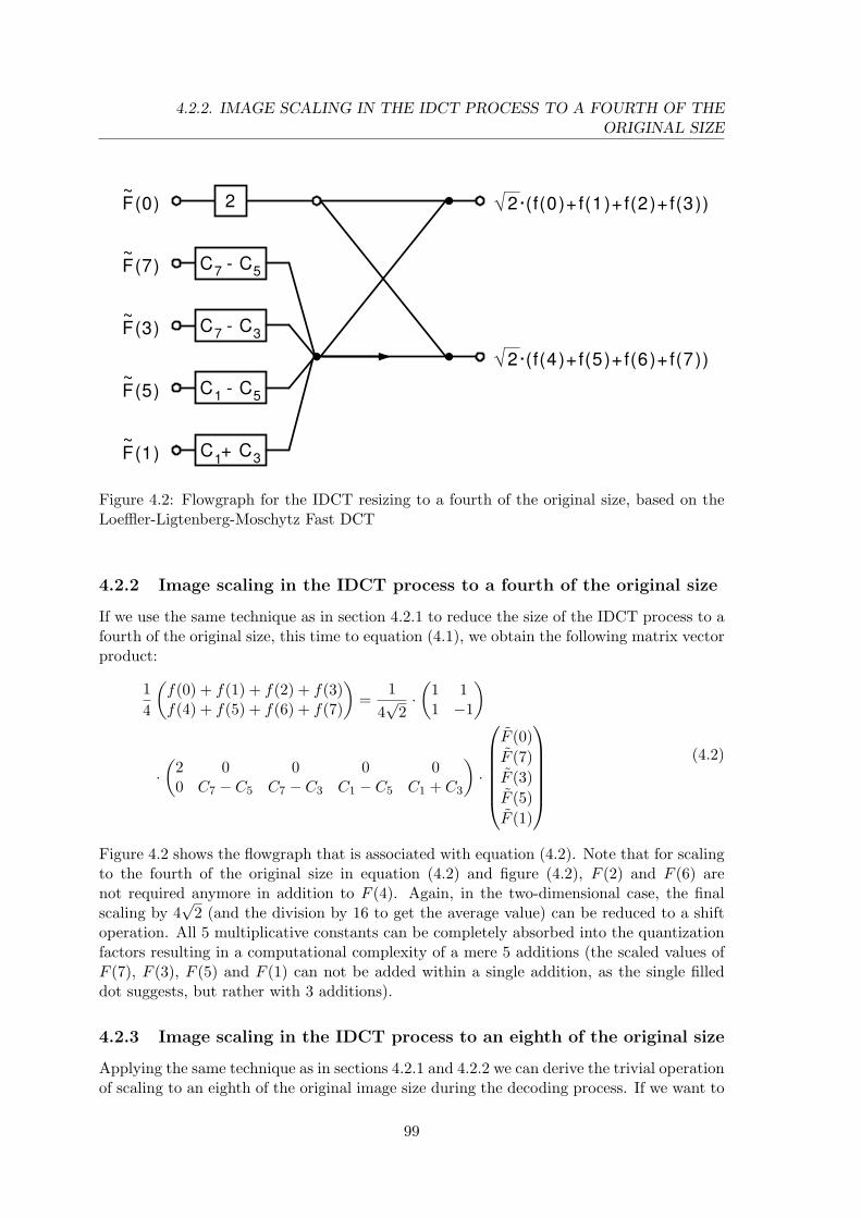
4.2.2. IMAGE SCALING IN THE IDCT PROCESS TO A FOURTH OF THEORIGINAL SIZE
F(0)
F(7)
F(3)
F(5)
F(1)
2·(f(0)+ f(1)+ f(2)+ f(3))2
C - C7 5
C - C7 3
C - C1 5
C + C1 3
2·(f(4)+ f(5)+ f(6)+ f(7))
~
~
~
~
~
Figure 4.2: Flowgraph for the IDCT resizing to a fourth of the original size, based on theLoeffler-Ligtenberg-Moschytz Fast DCT
4.2.2 Image scaling in the IDCT process to a fourth of the original size
If we use the same technique as in section 4.2.1 to reduce the size of the IDCT process to afourth of the original size, this time to equation (4.1), we obtain the following matrix vectorproduct:
14
(f(0) + f(1) + f(2) + f(3)f(4) + f(5) + f(6) + f(7)
)=
14√
2·(
1 11 −1
)
·(
2 0 0 0 00 C7 − C5 C7 − C3 C1 − C5 C1 + C3
)·
F (0)F (7)F (3)F (5)F (1)
(4.2)
Figure 4.2 shows the flowgraph that is associated with equation (4.2). Note that for scalingto the fourth of the original size in equation (4.2) and figure (4.2), F (2) and F (6) arenot required anymore in addition to F (4). Again, in the two-dimensional case, the finalscaling by 4
√2 (and the division by 16 to get the average value) can be reduced to a shift
operation. All 5 multiplicative constants can be completely absorbed into the quantizationfactors resulting in a computational complexity of a mere 5 additions (the scaled values ofF (7), F (3), F (5) and F (1) can not be added within a single addition, as the single filleddot suggests, but rather with 3 additions).
4.2.3 Image scaling in the IDCT process to an eighth of the original size
Applying the same technique as in sections 4.2.1 and 4.2.2 we can derive the trivial operationof scaling to an eighth of the original image size during the decoding process. If we want to
99

CHAPTER 4. FAST IMAGE SCALING IN THE CONTEXT OF JPEG DECODING
take the average of 8 adjacent pixels we simply have to add the two lines of the first matrixin equation (4.2):
18(f(0) + f(1) + f(2) + f(3) + f(4) + f(5) + f(6) + f(7)
)=
18√
2·(2 0
)
·(
2 0 0 0 00 C7 − C5 C7 − C3 C1 − C5 C1 + C3
)·
F (0)F (7)F (3)F (5)F (1)
=1
2√
2· F (0)
(4.3)
In the two-dimensional case, for an 8 × 8-block of pixels, this simply means dividing theDC-value by 8.
100

Chapter 5
The JPEGLib
Life’s most urgent question is: What are you doing for others?
– Martin Luther King
I never see what has been done; I only see what remains to be done.
– Madame Curie
The JPEGLib is a software library that is written and maintained by the IndependentJPEG Group (IJG). The Independent JPEG Group describes itself on its website
(http://www.ijg.org) as “an informal group that writes and distributes a widely used freelibrary for JPEG image compression”. The Independent JPEG Group has no real legalstatus or form of organization, nor is the group affiliated in any way with the ISO committeethat is responsible for the standardization of JPEG. Maybe it can best be described as agroup of individuals that are loosely connected via an internet mailing list and their officialwebsite, who voluntarily devote part of their time to the development and maintenance ofthe JPEGLib library.
In the following we will first give some historic retrospect and the design goals of thelibrary. This will be followed by a short description of the capabilities of the library that willshow what the user of the library can expect from it. We will continue with a descriptionof the package content and a description of the processes involved in building the library.This will include building the library for an already supported platform as well as portingthe library to a new platform as was the case in the project of this thesis. After that thetypical usage of the library and some architectural issues will be discussed, followed by asummary of the author’s experiences with the library which will conclude this chapter.
This chapter is not at all meant to serve as a replacement for the documentation thatcomes with the library package. The reader may consider this chapter as additional infor-mation that could help clarify things while reading along in the official documentation andmore or less reflects the author’s experiences from working mainly with the decompressionpart of the library. As an anticipation of the summary at the end of this chapter, the authorcould not find any serious flaws in the library, although there are some minor issues thatcould help improve performance and integratability of the library.
101

CHAPTER 5. THE JPEGLIB
5.1 Goals, Motivation and History
The IJG started their work on a library for JPEG compression and decompression at the endof 1990, at least this is what the earliest mailing list archive (http://www.ijg.org/archives)file suggests1. The initial goals of the group can be summarized by quoting from one ofthe earliest postings of Thomas G. Lane of Carnegie-Mellon University, moderator andorganizer of the group:
“. . . I see the main technical issues as:1. Making it work (getting the algorithms right);2. Making it portable (avoiding system dependencies);3. Making it fast.”
or more seriously, by quoting from the current version’s readme file:
“The emphasis in designing this software has been on achieving portabilityand flexibility, while also making it fast enough to be useful. In particular, thesoftware is not intended to be read as a tutorial on JPEG. [. . . ] Rather, it isintended to be reliable, portable, industrial-strength code.”
Another quote from Lane, this time from a usenet newsgroup posting in comp.graphics,alt.graphics.pixutils and other newsgroups from January 23rd of 1991, is sort of a “missionstatement” and puts things a bit more into the historical context of 1991:
“. . .We recognize that the net is not going to adopt any new posting formatunless free or very inexpensive software is available for a wide variety of ma-chines. We hope that we can cover enough machines to let JPEG reach “criticalmass” and become a de-facto standard on Usenet. Once that happens, peoplewith unusual hardware can adapt our source code to run on their machines.Another reason for our work is to encourage compatibility. The draft JPEGstandard is an extremely loose document: a large number of decisions are leftup to the individual implementor. People working in isolation are likely to pro-duce implementations that can’t actually exchange JPEG-format files. [. . . ] Bymaking and giving away a high-quality implementation, we hope to establish ade-facto standard for JPEG file format and to provide a painless path for peopleto adhere to that particular interpretation of the JPEG standard.”
Lane’s hope of the JPEGLib to “become a de-facto standard on Usenet” did not only cometrue, more important, with the Web revolution in the mid of the nineties, the JPEGLibbecame the de-facto standard for the World-Wide-Web. All major browser vendors up tonow use the code from the IJG for rendering JPEG images, including Netscape, the MozillaProject and Microsoft. Many other software packages such as Ghostscript, the libtiff libraryand numerous file conversion utilities use the IJG’s JPEGLib as well. One reason for this,besides from the exceptional quality, stability and performance of the code, are the verymodest licensing requirements which only require that the accompanying documentationmust state that “this software is based in part on the work of the Independent JPEG Group”if only executable code is distributed that makes use of the JPEGLib. Traditionally, the
1Note that this is actually more than one year prior to JPEG becoming an international standard, seesection 2.1.
102

5.2. CAPABILITIES OF THE JPEGLIB
Version Date Description
1 10/07/1991 First version, only JPEG baseline and extended-sequentialcompression processes supported, no progressive mode.
2 12/13/1991 Inclusion of config.c (later renamed to ckconfig.c), see section5.4, bugfixes and improved portability.
3 03/17/1992 “Swapping” memory manager, hooks for application UI re-flecting progress, two-pass color quantization for the decodingprocess, miscellaneous small speedups and bugfixes.
4 12/10/1992 Changes for improved accuracy, precision, speed and robust-ness, bugfixes and name changes.
4a 01/18/1993 Bugfixes and speedups.5 09/24/1994 Almost complete redesign and rewrite: Image scaling by a
factor of 1/2, 1/4, or 1/8 during the decoding process, com-plete change of the application programmer’s interface to thelibrary.
5a 12/07/1994 Better dithering and rounding, bugfixes.5b 03/15/1995 Bugfixes, better documentation.6 08/02/1995 Progressive mode support. New application “jpegtran” (see
section 5.3), small changes for application programmers.6a 02/07/1996 Robustness (versioning) and notation improved, small
changes in internal structures.6b 03/27/1998 Robustness improved, support for custom data in the com-
pression and decompression objects, markers can be pre-served in memory.
Table 5.1: Revision History of the JPEGLib
copyright owner of the IJG’s code is Thomas G. Lane, because the group worried that astatement like “copyright IJG” in the comments of the source code, with the IJG havingno real legal status, might be considered meaningless in a court of law if the IJG ever hadto try to enforce the copyright2.
Table 5.1 contains a short overview over the release history of the IJG’s JPEGLib, alongwith information about important changes.
5.2 Capabilities of the JPEGLib
The JPEGLib is a library written entirely in C that implements JPEG compression (en-coding) and decompression (decoding)3. The supported JPEG modes of operation (seesection 2.2.3) are the DCT-based sequential mode, in particular the baseline process, andthe progressive mode of operation with incremental decoding for on-the-fly display of pro-
2Today, with open-source copyrights pretty well understood, a lot of those early worries of the IJG seempointless in retrospect.
3Additionally, there are some assembler files available, either to make the library work on some platforms(MS-DOS) or in order to speed up critical operations.
103

CHAPTER 5. THE JPEGLIB
gressive images. The lossless and hierarchical modes of operation are not supported by theJPEGLib. As described in section 2.2, the JPEG standard does not fully specify an inter-changeable file format, therefore the JPEGLib follows the JFIF file format ([11]) which wasintroduced in section 2.3. The JPEGLib also does not support arithmetic coding, since thisis subject to several patents. Instead, Huffman encoding and decoding is implemented ina very close way to the coding propositions of the JPEG standards document ([5]). Thereare three different DCT implementations for both the FDCT and IDCT that are runtimeoptions: a slow but accurate floating-point variant using the Arai-Agui-Nakajima DCT (seesections 3.3.6 and 3.3.7), a faster yet slightly less accurate fixed-point variant using theLoeffler-Ligtenberg-Moschytz DCT (see sections 3.3.3 and 3.3.4), and a fast but much lessaccurate fixed-point variant using the Arai-Agui-Nakajima DCT. Additionally, specializedfixed-point algorithms based on the Loeffler-Ligtenberg-Moschytz DCT allow downscalingto the half, a fourth or to an eighth during decoding as described in sections 4.2.1, 4.2.2and 4.2.3. The JPEGLib is both able to support 8 bit and the rarely used 12 bit sampledata precision, but not simultaneously, since this is a compile-time decision. In addition todecoding into a 24-bit color format, the JPEGLib also contains a color decoding backendthat can create dithered output, using ordered dithering or Floyd-Steinberg dithering (seealso [10], [12], [16], [24] and [28]).
5.3 The JPEGLib package content
The JPEGLib source code and documentation comes as a compressed file that can bedownloaded from http://www.ijg.org/files/. The most current version at the time of writingis version 6b, dating from March 27th of 1998, and can be found at the aforementioned URLas the file jpegsrc.v6b.tar.gz. If this archive is unpacked, the files created can be roughlycategorized into the following 3 groups (see also the file filelist.doc that comes with thelibrary): JPEGLib core, sample applications and documentation. A detailed description ofevery file’s purpose can be found at the beginning of each source file. A brief description ofall files can be found in the file filelist.doc. As a simple file naming convention, every sourceand header file of the JPEGLib core starts with a “j” and the character following it in mostcases denotes the part to which this module belongs: If it is a “c”, the module belongs to thecompression/encoding part, if it is a “d”, the module belongs to the decompression/decodingpart of the library. Before a successful build of the library can be made, the library hasto be adapted to the specific environment where it is to be used. See section 5.4 and theJPEGLib’s file install.doc for more information on this topic.
When compiled successfully, a file named libjpeg.lib (the name may differ for differentplatforms or custom makefiles) and 3 sample applications are created whose purpose isdescribed as follows:
• cjpeg: A command-line utility to create JPEG files from different bitmap sourceformats.
• djpeg: A command-line utility to create different bitmap destination formats from aJPEG source file.
• jpegtran: A command-line utility for lossless transcoding from JPEG source files intoJPEG destination files of different formats.
104

5.4. ADAPTING THE JPEGLIB TO DIFFERENT PLATFORMS AND COMPILERS
5.4 Adapting the JPEGLib to different platforms andcompilers
As laid out before, the JPEGLib was written with portability across different environmentsin mind. This includes different computer architectures, operating systems and compilers.To account for these different environments, all compile-time relevant settings are collectedin one header file (jconfig.h) and are also reflected in the proper use of a suitable makefile.Proper use means here: The correct makefile has to be identified (or adapted from existingones) and edited to choose the correct memory manager for the environment in question.
5.4.1 Determining the correct jconfig.h file and the correct makefile
For popular non-Unix environments, preconfigured makefiles and header files are alreadysupplied, so making the JPEGLib ready to be successfully compiled takes only two steps:Renaming the right variant of jconfig.* to jconfig.h and renaming the right version of make-file.* to makefile (e.g. on a Win32 based system for the Microsoft C compiler, jconfig.vc isto be renamed to jconfig.h and makefile.vc is to be renamed to makefile). After that step,the JPEGLib is ready to be compiled by a make tool (i.e. the “nmake” tool in the afore-mentioned case of a Win32 based system and a Microsoft C compiler). This way, the mostimportant (and also some historical) non-Unix environments are covered, such as Amiga,Apple Macintosh, Atari ST, Digital VMS, Borland C on MS-DOS and OS/2, GNU C onMS-DOS, Microsoft C for MS-DOS and Win32 platforms, Watcom C on MS-DOS, Win32platforms and OS/2.
In the case of a Unix-like environment, the GNU C compiler is required and the twofiles are created by a shell script (configure).
For the not so popular environments like the one covered in this thesis, a tool can bebuilt that creates the jconfig.h file. For this purpose, the file named ckconfig.c needs to besuccessfully compiled into an executable. Running the executable then creates the jconfig.hfile. For the creation of jconfig.h, ckconfig.c works with some heuristics to determine thecorrect values for the jconfig.h file to be created. If the compilation of ckconfig.c fails, fixingthe cause of this error in ckconfig.c finally yields the correct result in the jconfig.h file tobe created. This way, a successful compilation of ckconfig.c finally creates a jconfig.h filefor the JPEGLib that is suitable for the environment under which ckconfig.c is compiled,and thus correct compile-time constants can be used for making the JPEGLib library. Thecompile-time constants mostly include properties of the compiler and Operating System(OS) in use, such as:
• Does the compiler or the OS use a flat memory model?
• Does the compiler use function prototypes?
• Does the compiler have the “boolean” data type?
• Does the compiler have unsigned variants of the char and short data type?
• Does the compiler use an unsigned right shift?
Since ckconfig.c creates a file, its usage is a bit problematic for embedded systems, wherethere typically is no file system available. In the case of this thesis, the code of ckconfig.c
105

CHAPTER 5. THE JPEGLIB
File name Description
jmemansi.c Swaps out data to unnamed temporary files using the ANSIstandard library routine tmpfile().
jmemname.c Swaps out data to named temporary files.jmemnobs.c Doesn’t swap out data to files(“nobs” in jmemnobs stands
for “No backing store”), relies on enough main or virtualmemory. Should compile on all platforms.
jmemdos.c Customized memory manager for MS-DOS.jmemdos.c Customized memory manager for the Apple Macintosh.
Table 5.2: Memory manager implementations supplied by the JPEGLib
was adapted to transmit the file content over the serial line, where it could be captured bya program running on the development system.
In very rare cases, such as the embedded system being used throughout this thesis, asecond header file, jmorecfg.h, needs to be adapted as well. In this file it is determined,among other things, what the preprocessor will evaluate for the pseudo-keyword FAR, thatis used within the JPEGLib for segmented architectures, like MS-DOS. Using this pseudo-keyword, different pointer arithmetics can be done on such platforms.
For a suitable makefile for the not so popular environments, two generic makefiles (make-file.ansi and makefile.unix) are provided as starting points for ANSI compliant compilersand compilers without function prototype support. In the case of this thesis, makefile.ansiwas choosen and adapted for the usage with the Cygnus port of the GNU make utility forWin32.
5.4.2 Choosing the right memory manager
The makefile for the JPEGLib always contains a variable named SYSDEPMEM which isassigned a value of one object file that contains the implementation of a memory manager.A memory manager for the JPEGLib assures that even on platforms with segmentation,such as MS-DOS or on systems with little memory, JPEG files can be encoded or decodedsuccessfully, even if the images are much bigger in size than the available memory of thesystem.
There are 5 different memory manager implementations provided with the JPEGLibwhich are implemented in the files given in table 5.2. If none of these memory managersfits for a particular purpose, a custom one can be written for a particular environment oran existing one can be adapted, as was the case with this thesis. Also, the SYSDEPMEMvariable in the makefile needs to be changed such that it points to the object file associatedwith the desired memory manager implementation.
Reasons for employing a memory manager scheme instead of the the naıve use of thestandard C-Runtime function malloc at all places where memory needs to be allocateddynamically, can be the following:
• On some systems, particularly segmented architectures such as MS-DOS or the em-bedded system used throughout this thesis, malloc simply sometimes cannot allocate
106

5.5. USAGE AND ARCHITECTURAL ISSUES
large enough memory buffers4 and therefore cannot always satisfy the requirementsof the caller.
• On some systems, OS system calls or calls into heap managers, e.g. when used in mul-tithreaded and SMP environments on more than one CPU, are much more efficientthan the standard C-runtime allocator malloc.
As a result, the JPEGLib’s memory manager uses two different allocator/deallocator func-tion pairs throughout its own code. The first one is jpeg get small and jpeg free small, whichare used for small blocks of memory. For bigger blocks of memory, the jpeg get large andjpeg free large functions are used5. Another advantage of the JPEGLib’s particular imple-mentation is, that all dynamic memory allocation that happens during encoding or decodingof one image is tracked in so-called “memory pools” that are associated with the compres-sion or decompression object6 and thus per-image data can be freed automatically in one fellswoop after this process by invoking one single cleanup function (jpeg finish compress andjpeg finish decompress). Also, all dynamic memory allocation that happens during encod-ing or decoding per one compression or decompression object can be freed automatically byinvoking one single cleanup function (jpeg destroy compress and jpeg destroy decompress).This way, the programmer does not need to bother about potential memory leaks insidethe library that could happen by not tracking all dynamically allocated memory.
5.5 Usage and Architectural Issues
This section will deal with a few design issues of the JPEGLib. The JPEGLib, thoughwritten in C, follows a few object-oriented principles that are well worth being explained.In particular this is inheritance, encapsulation via the usage of two fundamental compositedata types and polymorphism through function pointers. There are two reasons why thedevelopers of the JPEGLib preferred C over C++ for the implementation of their library:First, in the beginning of the nineties of the 20th century, using C was the only feasiblechoice for portable code and C++ was not yet well standardized. Secondly, the availablefree C++ compilers were neither very good7 nor widely portable.
Another reason could be to have chosen C as the least common denominator, becausevirtually all platforms have at least a more or less decent C compiler. This way also codewritten in other languages can use the IJG’s code either directly (e.g. C++ via the extern“C” keyword) or indirectly via dynamically linked libraries.
In the following we will first show what the typical code sequences are for encodingand decoding and will then proceed to the encoder and decoder objects and show howinheritance and polymorphism are achieved.
4The environment used throughout this thesis allows malloc to allocate only blocks up to a size of 214−1bytes, generally malloc can only allocate 2sizeof(size t) − 1 bytes, because the formal parameter of malloc isof type size t. For MS-DOS or the Win16 programming environment this is a mere 65535 bytes.
5A block allocated by jpeg get large also is a FAR pointer. Whether or not FAR is a special keywordand thus actually implies a special way of doing pointer arithmetics or whether it is simply expanded by theC preprocessor to nothing, depends on settings made in jconfig.h and jmorecfg.h.
6Compression and decompression in the JPEGLib involves a compression/decompression object that canbe reused for subsequent encoding or decoding processes of different images, see section 5.5.3.
7Even at the time of writing, C++ compiler implementations seem to be inherently flawed, whereaswriting good and efficient C compilers is a well researched topic for more more than 30 years.
107

CHAPTER 5. THE JPEGLIB
5.5.1 Typical code sequences for encoding
This section will show how typical code sequences will look like for the application developerwho wants to use the encoding part of the JPEGLib from within his code. We will adapt thepseudocode-like approach that is used in the library’s libjpeg.doc file and we will commenton the involved steps.
For the compression of images, the outline of the involved operations is as follows:
• Allocate and initialize a JPEG compression object.
• Specify the destination for the compressed data (e.g. a file).
• Set parameters for compression, including image size and colorspace.
• Call jpeg start compress(. . . );
• Do the following loop:while (scan lines remain to be written)
jpeg write scanlines(. . . );
• Call jpeg finish compress(. . . );
• Release the JPEG compression object.
The first step, allocating a JPEG compression object, is usually done by allocating it onthe stack, as an automatic variable. The size of such an object of type jpeg compress structon a 32-bit system is typically 360 bytes8, therefore on systems where the stack is a scarceresource because it has to fit into a single address segment of the microprocessor9, allocatingit on the stack could be a problem10. The initialization of the compression object is done byallocating an error manager object (jpeg error mgr) on the stack, assigning its address to amember of the compression object and by calling the macro jpeg create compress. The errorobject11 specifies the amount of diagnostic output during encoding via a so-called “TraceLevel”. It also contains function pointers as structure members that point to routines foremitting and formatting error and diagnostic messages12.
In case a JPEG file should be created, specifying the destination for the compresseddata is especially easy: Simply jpeg stdio dest needs to be called with a FILE* that wasopened for writing. In case the JPEG data should have a different destination, e.g. shouldbe transmitted over a serial line or written into memory or a memory-mapped-file, a so-called “destination manager” needs to be written. The interested reader will find moreinformation about this in the JPEGLib’s libjpeg.doc file.
Setting the parameters for compression consists merely of assigning values to membersof the compression object and calling the JPEGLib’s core function jpeg set defaults, which
8284 bytes on the embedded system in use throughout this thesis.9This is a problem for operating environments such as MS-DOS, Win16 or the system used throughout
this thesis.10In such cases the object must be allocated dynamically, i.e. via malloc. In this case, the programmer is
also responsible for releasing the object to the heap after usage.11The error object can be tailored to one’s own needs since a prototype is defined in the header file
jpeglib.h. This way the default function pointers can be overridden with pointers to own functions.12These messages usually come from a hardcoded message table, see jerror.h.
108

5.5.2. TYPICAL CODE SEQUENCES FOR DECODING
sets all members of the compression object to reasonable default values. Input colorspaceis set via the functions jpeg default colorspace or jpeg set colorspace13.
After calling jpeg start compress, a loop over all input scanlines must be performed,each time calling jpeg write scanlines with a pointer to a buffer of one or more lines of theinput image as the parameter.
A call to jpeg finish compress will now clean up all per-image data of the compres-sion object and a call to jpeg destroy compress will finally clean up all per-object data ofthe compression object. If the compression object was allocated on the stack, it will beautomatically released by leaving the current stack frame.
5.5.2 Typical code sequences for decoding
This section will show how typical code sequences will look like for the application developerwho wants to use the decoding part of the JPEGLib from within his code. Again, wewill adapt the pseudocode-like approach from the library’s libjpeg.doc file and we willcomment on the involved steps. For the decompression of images, a similar scheme to thatof compression is used. The outline of the involved operations is as follows:
• Allocate and initialize a JPEG decompression object.
• Specify the source of the compressed data (e.g. a file).
• Call jpeg read header() to obtain image information.
• Set parameters for decompression.
• Call jpeg start decompress(. . . );
• Do the following loop:while (scan lines remain to be read)
jpeg read scanlines(. . . );
• Call jpeg finish decompress(. . . );
• Release the JPEG decompression object.
The first step, allocating a JPEG decompression object, is usually done by allocating iton the stack, like the compression object in section 5.5.1. The size of such an object oftype jpeg compress struct on a 32-bit system is typically 432 bytes14, so again, allocatingit on the stack can be a problem in some environments. Similar to the steps involvedin compression, initialization of the decompression object is done by allocating an errormanager object on the stack, assigning its address to a member of the decompression objectand by calling the macro jpeg create decompress.
In case the source of compressed data is a file, the second step is quite easy: All thatneeds to be done is to supply a FILE* to a file that was opened for reading to the functionjpeg stdio src. In case JPEG data is in memory like it was the case in the project of thisthesis or is transmitted in pieces via the serial line, a so-called data source manager has tobe written for this purpose (see also the documentation in the JPEGLib’s file libjpeg.doc).
13Possible input color spaces are grayscale, YCbCr, RGB, CMYK, YCCK.14338 bytes on the embedded system in use throughout this thesis.
109

CHAPTER 5. THE JPEGLIB
The next step, calling jpeg read header, obtains useful information such as image re-solution and color space. This is particularly useful if memory is limited as it was in theproject of this thesis. At this point the decision was made whether to downscale the picturein the decoding process to half, to a fourth or to an eighth. In any case, knowing the hori-zontal resolution of the image allows the allocation of big-enough buffers for the line-by-lineprocessing in the while-loop that follows.
Setting parameters for decompression involves specifying which IDCT variant should beused or whether dithering should be used for color-quantized output.
After the call to jpeg start decompress, the while-loop is started and one or more linebuffers are passed with each call to jpeg read scanlines for decoding the image line by lineor several lines at once per call to jpeg read scanlines.
Like in the encoding process, a call to jpeg finish decompress will now clean up all per-image data of the decompression object and a call to jpeg destroy decompress will finallyclean up all per-object data of the compression object. If the decompression object wasallocated on the stack, it will be automatically released by leaving the current stack frame.
5.5.3 The encoder and decoder objects
The encoder and decoder objects are composite data types that are defined in the headerfile jpeglib.h. A composite data type in the C programming language is called a “struct”.A struct is similar to a class in C++ in that it supports some sort of encapsulation, butit does not support access specifiers like private, protected or public as in C++ or Java.A struct in C also has no notion of member functions15, let alone polymorphism, which isachieved in C++ through virtual member functions and is the default in Java. Also, C doesnot provide a builtin way to derive one struct from another to achieve inheritance. We willsee in the following, how the designers and implementors of the JPEGLib achieved thesefundamental principles of object-oriented design in C nevertheless:
The encoder and decoder objects both share a set of identical members which are atthe beginning of the binary layout of each object. This allows a pointer to a compressionor decompression object to be cast into a pointer to a struct jpeg common struct, whichcontains only those common members. This is an effective way of introducing inheritancein C and allows quite a lot of functions to operate on both encoder and decoder objects.If this were not the case, all the functions that take a pointer to a jpeg common structwould need to be duplicated: one variant for the compression object and another forthe decompression object. This way the structs for the encoder and decoder objects,jpeg compress struct and jpeg decompress struct, can be considered to be derived fromthe struct jpeg common struct.
Polymorphism in the JPEGLib is achieved in a very similar way to the way C++achieves this with virtual functions. In C++, each object that is of a class that has virtualfunctions or that is derived from a class with virtual functions, has a hidden member vari-able that points to a table with function pointers, the so-called “virtual function table”.The JPEGLib’s compression and decompression objects contain pointers to “managers” or“subobjects” that are responsible for different tasks during encoding or decoding, such asperforming the DCT, performing entropy encoding or decoding, color-conversion, upsam-pling or downsampling, etc. These “managers” in turn are again composite data types,
15Member functions are also often called “methods”.
110

5.6. SUMMARY
but most of them (see the header file jpegint.h) contain only function pointers and thushave the same functionality as the aforementioned virtual function tables16. By assigningthese function pointers different values, the functionality of the managers can be changedwithout changing the binary layout of the compression and decompression objects. Forinstance, selection of one of the three possible DCT variants per object consists of assigningone out of three functions with identical signature to the function pointer struct memberof the subobject that is responsible for doing the discrete cosine transform. Also, completemanagers can be replaced by custom managers, as long as the binary layout of the standardmanager is a subset of the custom manager, i.e. if the standard manager is of size n bytes,the custom manager must be at least of size n bytes and the first n bytes of both managersmust have the same meaning. This again, is nothing else than the concept of inheritance.
5.6 Summary
As a summary, the JPEGLib can be considered a modular and object-oriented library thatuses very elegant ways to achieve the fundamental principles of object-orientation despitethe fact that the C programming language has no intrinsic language support for these. Inaddition, by using subobjects within the two main types of objects for compression anddecompression, there is no deep hierarchy of inheritance, which circumvents the problemof “fragile base classes” as it is often encountered in deeply nested C++ class hierarchieswith overuse of polymorphism. Since the focus of this thesis was on the decoding part, thissummary also only covers the author’s experiences with this part of the library.
It turned out that the JPEGLib was the right choice for the purpose of decoding JPEGfiles on the embedded system used throughout the project of this thesis. The fact that thelibrary was written with a high degree of portability in mind made porting much easier.Especially the carefully written code parts for MS-DOS that via the pseudo-keyword FARallow different pointer arithmetics where this is necessary, made it possible to overcomethe limitations imposed by the segmentation of the microcontroller’s address space17. Alsothe modular architecture of the library made it possible to adapt for the requirements ofthis thesis’ project by using a custom data source manager that reads JPEG data frommain memory while accounting for the segmented architecture of the controller’s addressspace. Little effort was required to exchange other parts of the library by assigning newfunctions to the function pointers of various subobjects of the decompression object or evenby replacing complete subobjects with custom implementations.
Nevertheless a few observations could be made about potential improvements of thelibrary:
• The algorithms for the downscaled IDCTs to half and especially to a fourth of theoriginal image’s size (see sections 4.2.1 and 4.2.2) can be improved drastically byabsorbing the multiplicative factors for the dequantized DCT coefficients into thequantization tables. This way, e.g. for downscaling to a fourth, only additions arerequired and 5 multiplications per one row or column IDCT can be saved. Maybethe code of the JPEGLib uses these multiplications deliberately, because this way
16This concept is also known as the concept of Abstract data types. The parallels to “interfaces” as theyare used in CORBA, COM or Java is obvious.
17The microcontroller used throughout this thesis has a memory architecture that partitions the addressspace into so-called “pages” of size 214 bytes.
111

CHAPTER 5. THE JPEGLIB
better accuracy is achieved. But maybe it was just an oversight that the multiplicativeconstants like in the JPEGLib’s implementations of the Arai-Agui-Nakajima DCT canbe absorbed into the quantization table. At least for a few test images, no noticeabledifference could be found when using this optimization.
• The JPEGLib employs the row- and columnwise approach for all variants of the DCT.The following comment from the source code appears in a similar form in all modulesthat deal with the calculation of the DCT:
“A 2-D DCT can be done by 1-D DCT on each row followed by 1-DDCT on each column. Direct algorithms are also available, but they aremuch more complex and seem not to be any faster when reduced to code.”
The author considers this statement to be very questionable, since e.g. Feig’s algo-rithms for the scaled 2D FDCT and IDCT as described in sections 3.4.3 and 3.4.4require significantly less computational effort. A potential obstacle however for usingFeig’s algorithms in the JPEGLib could arise from patent issues: There is an indica-tion in Feig’s original article ([8]), that these algorithms are included in a U.S. patentapplication. Patent recherche showed that only one patent (patent number 5293434)was granted to Feig (and Pennebaker, one of the authors of [22]), that explicitly dealswith the 2D DCT, and it is unclear to the author whether it actually uses Feig’s 2DDCT as described in sections 3.4.3 and 3.4.4. Also: This patent was filed in 1991,Feig’s original article ([8]) dates back to 1990 and states that the patent was alreadyfiled way back in 1989.
• For an embedded system it makes no sense to have diagnostic messages or errormessages during decoding an image, because there is no command prompt or othermeans for displaying such output. There are only two alternatives: either decodingsucceeds or it fails, in which case it is sufficient to show to the user that there wasa problem, but not which problem. Therefore it would have been a good idea if theimplementors of the JPEGLib had made diagnostic and error output a compile-timeoption. In the case of this thesis, some measurable improvement could be made bysimply expanding the macros WARNMS,TRACEMS, . . . in the header file jerror.h tonothing. Further improvement could probably be made by incorporating both thecondition check for a diagnostic message and the ID for the diagnostic message intoa macro which simply expands to nothing if this compile-time option is not used.This way those applications that use diagnostic output could continue to use it, whilefor others both the condition check and the diagnostic output could be completelyomitted, resulting in higher performance. It could be argued, that users should writetheir own error handling code, but including this into the default error handler wouldnot hurt and would relieve users from tinkering with an own error handler.
• Even in the case that errors and warnings and other diagnostic output is desired,the suggestion in libjpeg.doc under “Error handling” to override some of the methodpointers in the jpeg error mgr struct after calling jpeg std error() is not really helpfulas to internationalization and localization. Even in this case, error messages still comefrom the file jerror.h as ANSI strings in plain English. But not all the world is Englishand in the age of UNICODE, ANSI strings more and more appear to be some sortof an anachronism. Again it could be argued, that users should write their own error
112

5.6. SUMMARY
handler, but few if any users will probably do this. Most users will probably stickwith the hardcoded error messages from jerror.h in ANSI and plain English, thereforethe author’s view is, that the default error manager should be made more flexible andextensible to account for the aforementioned issues.
• Overuse of macros: During the phase of porting the JPEGLib to the microcontrollerused during this thesis, an occasional error occurred during the decoding process inthe macro HUFF DECODE in the source file jdhuff.c. The macro HUFF DECODEturned out to be the following monster (see header file jdhuff.h):
#define HUFF_DECODE(result,state,htbl,failaction,slowlabel) \
{ register int nb, look; \
if (bits_left < HUFF_LOOKAHEAD) { \
if (! jpeg_fill_bit_buffer(&state,get_buffer,bits_left, 0)) {failaction;} \
get_buffer = state.get_buffer; bits_left = state.bits_left; \
if (bits_left < HUFF_LOOKAHEAD) { \
nb = 1; goto slowlabel; \
} \
} \
look = PEEK_BITS(HUFF_LOOKAHEAD); \
if ((nb = htbl->look_nbits[look]) != 0) { \
DROP_BITS(nb); \
result = htbl->look_sym[look]; \
} else { \
nb = HUFF_LOOKAHEAD+1; \
slowlabel: \
if ((result=jpeg_huff_decode(&state,get_buffer,bits_left,htbl,nb)) < 0) \
{ failaction; } \
get_buffer = state.get_buffer; bits_left = state.bits_left; \
} \
}
Note that the author does not object against the coding style of this snippet or theusage of “goto”18, it simply is impossible to debug something like that19. In addition,PEEK BITS and DROP BITS used in this macro are again macros. This code had tobe expanded manually by the author of this thesis in order to find and fix the error.
It can be considered a matter of taste or performance whether this code should ratherbe a function or a macro. If performance is the reason for implementing it as a macro,the author of this thesis would probably have written this as normal code instead ofa macro, given the fact that this macro is invoked only 6 times.
18Despite the doctrine “goto considered harmful” ([7]), goto is the right choice when it comes up toperformance as in this library or in C-runtime libraries.
19The C preprocessor expands the whole macro to a single line.
113

Chapter 6
JPEG Decoding on the MicronasSDA 6000 Controller
Don’t you know you fool, you never can win?Use your mentality, wake up to reality.
– From the song “I’ve got you under my skin” by Cole Porter(from the movie “Born To Dance”, 1936)
This chapter contains the results of the project pursued throughout this thesis. Forthe maintainer of the code base that was developed, it contains a description of the
projects used for decoding on the SDA 6000 controller as well as a detailed description of thechanges to the JPEGLib, that were required to make the JPEGLib run on this hardware.The aim of these sections is to give the maintainer of the source code explanations to thecode changes and they can be probably best understood while using a tool that shows thedifferences between the standard JPEGLib, as distributed by the IJG, and the code writtenthroughout this thesis. Following this will be a section that explains the changes to theJPEGLib for a modified version of the IDCT algorithm that scales the image to a fourth,as suggested in section 4.2.2. The sections following this are descriptions of the custommanagers that were written to replace parts of the JPEGLib. and finally an overview ofthe actual performance that is possible with the SDA 6000 controller.
6.1 Project descriptions
The controller being used throughout this thesis is the SDA 6000 from Micronas, Munich.The controller’s code name during its development was “M2” and this name has beenretained until the time of writing, even in official documentation. Therefore and for thesake of brevity, we will use the controller’s code name in the following.
For the decoding of JPEG files on the M2, two projects exist that can both be used forfurther development. Both projects compile cleanly without any warnings or errors in thehighest warning level, besides from third-party code. Both require the toolchain “TASKINGC/C++ for C166/ST10 v7.0 r1” from Tasking Inc. and reside under the corporate-wideprescribed directory d:\work in separate directories:
114

6.2. CHANGES TO THE JPEGLIB
• Under d:\work\ae7 a project can be found that initially served as the starting point inthat it contained routines for drawing on the TV screen with the primitives from theGraphics Device Interface (GDI) of the M2. This project was mainly used during thephase of porting the JPEGLib to the M2. In this project, the JPEG decoder part isrunning concurrently with other processes under the real-time operating system OSE.The associated project file can be found under d:\work\ae7\as the file AE7.psp. Thebinary that is created by a successful build of this project is the file ae7.out in thesame directory. After the need was encountered to abandon the operating system forperformance reasons, this project was superseded by the second project.
• The second project is located under d:\work\mini and emerged from an OS-lessproject, named “warmup” that was provided courtesy of Micronas, the manufacturerof the M2. This project allows the JPEG decoder to run at maximum performanceas a single task on the M2 without any underlying OS. Additionally, it can be com-piled to use either the standard GDI for the M2 in 4-4-4 mode or the experimental“MINI GDI”1 that switches the M2 into 5-6-5 mode. The associated project file canbe found under d:\work\mini\target\warmup\Tasking as the file Warmup.pjt. Thebinary that is created by a successful build of this project is the file warmup.out inthe same directory.
Both projects are built via the Integrated Development Environment that ships with thetoolchain.
6.2 Changes to the JPEGLib
Both projects use the same copy of the JPEGLib which was slightly modified duringthe porting phase to adapt to this previously unsupported platform. This variant of theJPEGLib can be found in the following directory:d:\work\ae7\V601 EvalBoard\FunctionLibrary\Functions\jpeglib.The binary image of the library itself is the file libjpeg.lib. In order to successfully buildthe library a command console must be started and the current directory must be changedto this directory, followed by invoking “make”. The suggested make utility comes fromthe Cygnus port of the GNU compiler for Win32. A custom jconfig.h was created fromckconfig.h and the library’s makefile.ansi was modified and used as the library’s makefileas described in section 5.4. The JPEGLib had to be modified at surprisingly few places inorder to run on the M2. In order to get it compiled, actually no changes were required.However, it turned out that the standard memory manger (memnobs.c) could not allocatelarge enough blocks, so it was modified accordingly. The following changes to the memorymanager were required:
• Two global function pointers were introduced that have identical function signaturesto the standard allocator/deallocator pair malloc and free in jconfig.h:
#include <stdio.h> //for definition of data type size_t
typedef void* (*memalloc)(size_t);
extern memalloc g_fnMemAlloc;
1The MINI GDI library was supplied halfway through during this thesis from Tara Systems, the vendorfor the official GDI. For information on how to work with it see [17].
115

CHAPTER 6. JPEG DECODING ON THE MICRONAS SDA 6000 CONTROLLER
typedef void (*memfree)(void *);
extern memfree g_fnMemFree;
The implementation and initialization of these global function pointers can be foundin the modified variant of jmemnobs.c:
memalloc g_fnMemAlloc = NULL;
memfree g_fnMemFree = NULL;
• A custom implementation of jpeg get large and jpeg free large (see section 5.4.2) wasmade in jmemnobs.c:
GLOBAL(void FAR *)
jpeg_get_large (j_common_ptr cinfo, size_t sizeofobject)
{
if (g_fnMemAlloc)
return (void FAR *) g_fnMemAlloc(sizeofobject);
else
return NULL;
}
GLOBAL(void)
jpeg_free_large (j_common_ptr cinfo, void FAR * object, size_t sizeofobject)
{
if (g_fnMemFree)
g_fnMemFree(object);
}
By using these function pointers, the actually used allocator could be set from outside.This happens in the files GraphicsDemo.cpp underd:\work\ae7\V601 EvalBoard\FunctionLibrary\Functions\jpeg\Src and in the filestartup.c under d:\work\mini\target\warmup\Source where these function pointersare assigned the addresses of the functions MemoryAlloc and MemoryFree whose im-plementation can be found in the file memalloc.c in the directoryd:\work\ae7\V601 EvalBoard\FunctionLibrary\Functions\jpeg\Src.
The implementations of MemoryAlloc and MemoryFree are as follows:
void * MemoryAlloc (size_t st)
{
XHandle h = GdiAllocMemory(st+sizeof(XHandle), 0x80, GDI_ALLOC_USE_GAPS);
if (GDI_NULL_HANDLE != h)
{
unsigned char huge *lp = (unsigned char *)GdiLockMemory(h);
memcpy((void *)lp, (void *)&h, sizeof(XHandle));
lp = &lp[sizeof(XHandle)];
return (void *)lp;
}
else
return NULL;
}
116

6.2. CHANGES TO THE JPEGLIB
void MemoryFree (void *p)
{
XHandle x;
unsigned char huge *lp = (unsigned char *)p;
lp -= sizeof(XHandle);
x = *((XHandle *)lp);
GdiUnlockMemory(x);
GdiFreeMemory(x);
}
MemoryAlloc allocates with the help of the GDI routines (which can allocate much morememory than the standard allocator malloc) memory that is exactly the size of an XHandlelarger than required. The memory handle that is returned from the library is then lockedand the value of the memory handle is written at the beginning of this piece of lockedmemory. The address that starts after this location is then returned to the caller andis exactly the size the caller requested. MemoryFree first determines the address wherethe value of the associated handle can be found by decrementing the supplied address bysizeof(XHandle), stores this value in a temporary variable and unlocks and releases thememory via this variable. With this scheme via function pointers, the GDI library can lendits capability to allocate big amounts of memory to the JPEGLib without the necessity tomerge these libraries or make them too dependent on each other. In order for the JPEGLibto account for the segmented architecture of the M2, jmorecfg.h had to be changed as wellso the pseudo-keyword FAR is replaced by the C preprocessor with “huge”:
#ifdef NEED_FAR_POINTERS
#define FAR huge
#else
#define FAR
#endif
Of course, for this to work, NEED FAR POINTERS in jconfig.h has to be defined as well:
#define NEED_FAR_POINTERS
Additionally, the JPEGLib needs a primitive for copying data blocks, taking into accountthe segmented architecture of the M2. This is done by specifying the macro FMEMCOPYin jconfig.h:
#define FMEMCOPY(dest,src,size) memcphhb((void huge *)(dest), \
(const huge FAR *)(src), (size_t)(size))
The function memcphhb is a variant for the standard C-runtime function memcpy thattakes “huge Pointers” as arguments, thus it does 32-bit pointer arithmetics instead of theM2’s standard 14-bit pointer arithmetics.
The real difficulty in getting the JPEGLib to work was to provide a custom data sourcemanager. Section 6.5 will elaborate on this topic. For now we will continue with the changesmade to the JPEGLib.
The JPEGLib employs a function (jzerofar) in jutils.c that initializes memory with ze-roes. This can be either defined via a macro (FMEMZERO) as in the case of FMEMCOPY,otherwise via a slow method that initializes the memory byte-by-byte with slow FAR pointerarithmetics. For the M2 there is no runtime primitive for that purpose, a faster variant couldbe found by separating the memory in pages and using faster standard pointer arithmetics:
117

CHAPTER 6. JPEG DECODING ON THE MICRONAS SDA 6000 CONTROLLER
GLOBAL(void)
jzero_far (void FAR * target, size_t bytestozero)
/* Zero out a chunk of FAR memory. */
/* This might be sample-array data, block-array data, or alloc_large data. */
{
#ifdef FMEMZERO
FMEMZERO(target, bytestozero);
#else
/* // Standard implementation. Slow, uses FAR ptrs:
register char FAR * ptr = (char FAR *) target;
register size_t count;
for (count = bytestozero; count > 0; count--) {
*ptr++ = 0;
*/
// We first determine the number of bytes that are left till the beginning
// of the next page in variable iRemainder. Then we zero out either bytestozero
// bytes (if bytestozero<iRemainder) and return, or we zero out the rest of the
// current page.
// At that point we set ptr to the beginning of the next page and decrement
// bytestozero by the number of bytes we already zeroed out. From this moment on
// iRemainder is always the size of one page (0x4000). Then we’ll start all over
// again the whole thing.
register char * ptr = (char *) target;
register unsigned int iRemainder = 0x4000 - ((unsigned int)ptr)%0x4000;
register size_t count;
for (;;)
{
if (bytestozero<iRemainder)
{
for (count = bytestozero; count > 0; count--)
*ptr++ = 0;
return;
}
else
{
for (count = iRemainder; count > 0; count--)
*ptr++ = 0;
}
target = (void FAR *)((char FAR *)target+iRemainder);
ptr = (char *) target;
// now ptr is exactly on the start of a new page.
bytestozero -= iRemainder;
iRemainder = 0x4000;
}
#endif
}
As the comment points out, this implementation first calculates the number of bytes untilthe next page starts and zeroes out these or the maximum number of bytes. This can bedone with a normal pointer (as opposed to a huge pointer), because no page boundary is
118

6.2. CHANGES TO THE JPEGLIB
crossed. Then the pointer is assigned the address of the next page and again the numberof bytes until the next page or the maximum number of bytes are zeroed out until no morebytes to zero are left.
In order to keep the binary as small as possible (and so compile and link cycles), severaloptions in the file jmorecfg.h were turned off2:
#undef DCT_FLOAT_SUPPORTED /* floating-point: accurate, fast on fast HW */
#undef C_PROGRESSIVE_SUPPORTED /* Progressive JPEG? (Requires MULTISCAN)*/
#undef D_PROGRESSIVE_SUPPORTED /* Progressive JPEG? (Requires MULTISCAN)*/
#undef SAVE_MARKERS_SUPPORTED /* jpeg_save_markers() needed? */
#undef BLOCK_SMOOTHING_SUPPORTED /* Block smoothing? (Progressive only) */
#undef QUANT_1PASS_SUPPORTED /* 1-pass color quantization? */
#undef QUANT_2PASS_SUPPORTED /* 2-pass color quantization? */
In the case of QUANT 1PASS SUPPORTED things are a bit complicated: For dithering,this macro must be defined. For undithered output it is not required and has a negativeeffect on performance. Enabling dithering is a compile-time option (see section ). The lastoptimization to be done in jmorecfg.h is to define a data type for fast multiplication:
#ifndef MULTIPLIER
#define MULTIPLIER short /* type for fastest integer multiply */
#endif
For performance reasons, as described in section 5.6, diagnostic output was made acompile time decision by introducing a macro DEBUG. In case DEBUG is defined, theJPEGLib does normal diagnostic output, in case it is not defined, the macros WARNMS,WARNMS1, WARNMS2, TRACEMS, TRACEMS1, . . . TRACEMS8 and TRACEMSS sim-ply expand to nothing:
#define WARNMS(cinfo,code)
#define WARNMS1(cinfo,code,p1)
#define WARNMS2(cinfo,code,p1,p2)
#define TRACEMS(cinfo,lvl,code)
#define TRACEMS1(cinfo,lvl,code,p1)
#define TRACEMS2(cinfo,lvl,code,p1,p2)
#define TRACEMS3(cinfo,lvl,code,p1,p2,p3)
#define TRACEMS4(cinfo,lvl,code,p1,p2,p3,p4)
#define TRACEMS5(cinfo,lvl,code,p1,p2,p3,p4,p5)
#define TRACEMS8(cinfo,lvl,code,p1,p2,p3,p4,p5,p6,p7,p8)
#define TRACEMSS(cinfo,lvl,code,str)
In order to get diagnostic output during debugging over the serial line of the M2 board,jerror.c was modified. Again a global function pointer (jprintffunc), this time with thefunction signature of the well-known function printf was implemented as well as a functionfor diagnostic output (jprintf). This function could either be called separately or from theerror managers output message function, which was modified to call jprintf:
2Besides from reducing the makefile to the decode part only.
119

CHAPTER 6. JPEG DECODING ON THE MICRONAS SDA 6000 CONTROLLER
#include <stdio.h>
#include <stdarg.h>
#ifdef JPRINTF
pprintf jprintffunc= NULL;
char szBuf [1024];
int jprintf ( const char * format, ... )
{
va_list arglist;
va_start(arglist, format);
vsprintf(szBuf, format, arglist);
if (jprintffunc)
return jprintffunc(szBuf);
else
return 0;
}
#endif
METHODDEF(void)
output_message (j_common_ptr cinfo)
{
#ifdef _DEBUG
char buffer[JMSG_LENGTH_MAX];
/* Create the message */
(*cinfo->err->format_message) (cinfo, buffer);
#ifdef USE_WINDOWS_MESSAGEBOX
/* Display it in a message dialog box */
MessageBox(GetActiveWindow(), buffer, "JPEG Library Error",
MB_OK | MB_ICONERROR);
#else
/* Send it to stderr, adding a newline */
#ifdef JPRINTF // we do a custom printf across the serial line for the M2
jprintf("%s\n", buffer);
#endif
#endif
#endif
}
Of course, for this to work, JPRINTF must be defined in jconfig.h and pprintf typedef’ed;
#define JPRINTF // jprintf function defined or not?
#ifdef JPRINTF //defined in jconfig.h
typedef int (*pprintf)(const char *);
extern pprintf jprintffunc;
int jprintf ( const char *, ... );
#endif
To make this diagnostic functionality actually work, the function pointer jprintffunc nowneeds to be assigned a value of a function with a signature that resembles printf’s signature.This is done in the file jdecode.c in the function JpegDecode. The actual implementationof this function calls code that transmits the diagnostic output via the serial line of the M2board to a monitoring program on the development computer via third-party code.
120
6.3. CHANGES FOR FASTER DOWNSCALING TO A FOURTH
A slight performance boost came from using the M2’s IRAM data for tables that areused during Huffman decoding. By qualifying these tables with the keyword iram thelinker/locator puts them into IRAM:
int _iram extend_test[16] = /* entry n is 2**(n-1) */
{ 0, 0x0001, 0x0002, 0x0004, 0x0008, 0x0010, 0x0020, 0x0040, 0x0080,
0x0100, 0x0200, 0x0400, 0x0800, 0x1000, 0x2000, 0x4000 };
int _iram extend_offset[16] = /* entry n is (-1 << n) + 1 */
{ 0, ((-1)<<1) + 1, ((-1)<<2) + 1, ((-1)<<3) + 1, ((-1)<<4) + 1,
((-1)<<5) + 1, ((-1)<<6) + 1, ((-1)<<7) + 1, ((-1)<<8) + 1,
((-1)<<9) + 1, ((-1)<<10) + 1, ((-1)<<11) + 1, ((-1)<<12) + 1,
((-1)<<13) + 1, ((-1)<<14) + 1, ((-1)<<15) + 1 };
The qualifiers “static” and “const” were removed, in order to verify that these tables actuallywere created in IRAM address space via the map file. For experimental purposes in thisfile also memory allocation in jpeg make d derived tbl uses different allocators dependingon the value of the macro HUFF LOOKAHEAD. It turned out that a higher value ofHUFF LOOKAHEAD than its default (8) can accelerate Huffman decoding, but also forsome images allocation requests could not be satisfied, so the default value is probably thesafest way to go. In order to “hook” into Huffman decoding with own functions (see section), function start pass huff decoder had to be made publicly available, so the METHODDEFmacro (which expands to “static”) had to be removed for this function.
In order to improve the Arai-Agui-Nakajima IDCT the keyword “const” was removedfrom a local dequantization table (aanscales) in jddctmgr.c in the function start pass. Ifconst is applied to a variable, this variable is placed into the ROM and is then first copiedinto RAM when it is used. By removing const, this step can be omitted, resulting in higherperformance.
6.3 Changes for faster downscaling to a fourth
As explained in section 4.2.2, the algorithm to downscale to a fourth can make use ofabsorbing the constant multiplication factors into the dequantization tables. The actualimplementation of this turned out to be dependent on the target platform, and maybe thisis why the authors of the JPEGLib did not favor this improvement. Different multiplicationtables for the dequantization tables are required for 16-bit and 32-bit platforms and espe-cially for 16-bit platforms such as the M2, this leads to reduced accuracy. In order to turnon the new functionality, the macro USE FASTER 2x2 IDCT must be defined in jconfig.h:
#define USE_FASTER_2x2_IDCT
In jddctmgr.c now the two tables are defined with the macros SLOPPY16BITTABLEand ACCURATETABLE:
121

CHAPTER 6. JPEG DECODING ON THE MICRONAS SDA 6000 CONTROLLER
/*
Table for decoding to the fourth on 16-bit platforms
with very unaccurate results:
*/
#define SLOPPY16BITTABLE 32, 29, 16, 10, 16, 7, 16, 6,\
29, 26, 14, 9, 14, 6, 14, 5,\
16, 14, 8, 5, 8, 3, 8, 3,\
10, 9, 5, 3, 5, 2, 5, 2,\
16, 14, 8, 5, 8, 3, 8, 3,\
7, 6, 3, 2, 3, 1, 3, 1,\
16, 14, 8, 5, 8, 3, 8, 3,\
6, 5, 3, 2, 3, 1, 3, 1\
/*
Table for decoding to the fourth on all other platforms
with accurate results:
*/
#define ACCURATETABLE 2097152, 1900287, 1048576, 667292, 1048576, 445870, 1048576, 377991,\
1900287, 1721902, 950143, 604652, 950143, 404015, 950143, 342508,\
1048576, 950143, 524288, 333646, 524288, 222935, 524288, 188995,\
667292, 604652, 333646, 212325, 333646, 141871, 333646, 120273,\
1048576, 950143, 524288, 333646, 524288, 222935, 524288, 188995,\
445870, 404015, 222935, 141871, 222935, 94795, 222935, 80364,\
1048576, 950143, 524288, 333646, 524288, 222935, 524288, 188995,\
377991, 342508, 188995, 120273, 188995, 80364, 188995, 68129
These two tables contain the constant factors for the algorithm of downscaling to a fourthfrom section 4.2.2 for fixed point arithmetics. SLOPPY16BITTABLE uses 3-bit fixedpoint arithmetics, which means that the constant factors are scaled with 23 = 8 whereasACCURATETABLE uses 19-bit fixed point arithmetics, which means that the constantfactors are scaled with 219 = 524288. It can easily be shown that these two values lead tothe maximum accuracy for 16-bit and 32-bit platforms without leading to an overflow. Thefloating point values that represent the factors from the algorithm in section 4.2.2 whichlead to these two tables are the following:
4.000000 ,3.624510 ,2.000000 ,1.272759 ,2.000000 ,0.850430 ,2.000000 ,0.720960 ,
3.624510 ,3.284268 ,1.812255 ,1.153281 ,1.812255 ,0.770598 ,1.812255 ,0.653281 ,
2.000000 ,1.812255 ,1.000000 ,0.636379 ,1.000000 ,0.425215 ,1.000000 ,0.360480 ,
1.272759 ,1.153281 ,0.636379 ,0.404979 ,0.636379 ,0.270598 ,0.636379 ,0.229402 ,
2.000000 ,1.812255 ,1.000000 ,0.636379 ,1.000000 ,0.425215 ,1.000000 ,0.360480 ,
0.850430 ,0.770598 ,0.425215 ,0.270598 ,0.425215 ,0.180808 ,0.425215 ,0.153281 ,
2.000000 ,1.812255 ,1.000000 ,0.636379 ,1.000000 ,0.425215 ,1.000000 ,0.360480 ,
0.720960 ,0.653281 ,0.360480 ,0.229402 ,0.360480 ,0.153281 ,0.360480 ,0.129946
In order to do the actual implementation of absorbing these tables into the dequantizationvalues the following code must be added to the function start pass in jddctmgr.c:
122

6.3. CHANGES FOR FASTER DOWNSCALING TO A FOURTH
#ifdef PROVIDE_ISLOW_TABLES
case JDCT_ISLOW:
{
/* For LL&M IDCT method, multipliers are equal to raw quantization
* coefficients, but are stored as ints to ensure access efficiency.
*/
ISLOW_MULT_TYPE * ismtbl = (ISLOW_MULT_TYPE *) compptr->dct_table;
if (method_ptr != jpeg_idct_2x2)
{
for (i = 0; i < DCTSIZE2; i++)
{
ismtbl[i] = (ISLOW_MULT_TYPE) qtbl->quantval[i];
}
}
else
{
#ifdef USE_FASTER_2x2_IDCT
static const INT32 iTwoByTwoScales[DCTSIZE2] =
{
#if (INT_MAX==32767)
SLOPPY16BITTABLE
#else
ACCURATETABLE
#endif
};
for (i=0;i<DCTSIZE2;i++)
ismtbl[i] = (ISLOW_MULT_TYPE)((INT32) qtbl->quantval[i] *
(INT32) iTwoByTwoScales[i]);
#else //USE_FASTER_2x2_IDCT
for (i = 0; i < DCTSIZE2; i++)
{
ismtbl[i] = (ISLOW_MULT_TYPE) qtbl->quantval[i];
}
#endif
}
}
break;
#endif
This piece of code checks whether the downscaling should be downscaling to a fourth (if(method ptr != jpeg idct 2x2). . . ). If so, the dequantization tables are multiplied witheither SLOPPY16BITTABLE or ACCURATETABLE. The detection of the platform isdone with checking the value of the standard C macro INT MAX. If INT MAX evaluatesto 32767, it is a 16-bit platform. For this to work, the standard header limits.h must beincluded at the beginning of the file:
#include <limits.h> /*for INT_MAX*/
This header file must be included in the same way in jidctred.c because in this file thealternative variant of the function jpeg idct 2x2 is implemented. Depending on the valueof the macro USE FASTER 2x2 IDCT the preprocessor uses the appropriate version injidctred.c like in the following:
123

CHAPTER 6. JPEG DECODING ON THE MICRONAS SDA 6000 CONTROLLER
#ifndef USE_FASTER_2x2_IDCT
GLOBAL(void)
jpeg_idct_2x2 (j_decompress_ptr cinfo, jpeg_component_info * compptr,
JCOEFPTR coef_block,
JSAMPARRAY output_buf, JDIMENSION output_col)
{
/* standard implementation that comes with the JPEGLib */
.....
}
#else
GLOBAL(void)
jpeg_idct_2x2 (j_decompress_ptr cinfo, jpeg_component_info * compptr,
JCOEFPTR coef_block,
JSAMPARRAY output_buf, JDIMENSION output_col)
{
/* new, faster implementation with constants absorbed in dequantization table */
.....
}
#endif
The complete implementation of the faster variant of jpeg idct 2x2 is the following.
GLOBAL(void)
jpeg_idct_2x2 (j_decompress_ptr cinfo, jpeg_component_info * compptr,
JCOEFPTR coef_block,
JSAMPARRAY output_buf, JDIMENSION output_col)
{
int tmp0, tmp10, z1;
JCOEFPTR inptr;
ISLOW_MULT_TYPE * quantptr;
int * wsptr;
JSAMPROW outptr;
JSAMPLE *range_limit = IDCT_range_limit(cinfo);
int ctr;
int workspace[DCTSIZE*2]; /* buffers data between passes */
SHIFT_TEMPS
/* Pass 1: process columns from input, store into work array. */
inptr = coef_block;
quantptr = (ISLOW_MULT_TYPE *) compptr->dct_table;
wsptr = workspace;
for (ctr = DCTSIZE; ctr > 0; inptr++, quantptr++, wsptr++, ctr--) {
/* Don’t bother to process columns 2,4,6 */
if (ctr == DCTSIZE-2 || ctr == DCTSIZE-4 || ctr == DCTSIZE-6)
continue;
if (inptr[DCTSIZE*1] == 0 && inptr[DCTSIZE*3] == 0 &&
inptr[DCTSIZE*5] == 0 && inptr[DCTSIZE*7] == 0) {
/* AC terms all zero; we need not examine terms 2,4,6 for 2x2 output */
int dcval = DEQUANTIZE(inptr[DCTSIZE*0], quantptr[DCTSIZE*0]);
wsptr[DCTSIZE*0] = dcval;
wsptr[DCTSIZE*1] = dcval;
continue;
}
124

6.3. CHANGES FOR FASTER DOWNSCALING TO A FOURTH
/* Even part */
z1 = DEQUANTIZE(inptr[DCTSIZE*0], quantptr[DCTSIZE*0]);
tmp10 = z1;
/* Odd part */
z1 = DEQUANTIZE(inptr[DCTSIZE*1], quantptr[DCTSIZE*1]);
tmp0 = z1;
z1 = DEQUANTIZE(inptr[DCTSIZE*5], quantptr[DCTSIZE*5]);
tmp0 += z1;
z1 = DEQUANTIZE(inptr[DCTSIZE*3], quantptr[DCTSIZE*3]);
tmp0 -= z1;
z1 = DEQUANTIZE(inptr[DCTSIZE*7], quantptr[DCTSIZE*7]);
tmp0 -= z1;
/* Final output stage */
wsptr[DCTSIZE*0] = (int) ((tmp10 + tmp0));
wsptr[DCTSIZE*1] = (int) ((tmp10 - tmp0));
}
/* Pass 2: process 2 rows from work array, store into output array. */
wsptr = workspace;
for (ctr = 0; ctr < 2; ctr++) {
outptr = output_buf[ctr] + output_col;
/* It’s not clear whether a zero row test is worthwhile here ... */
#ifndef NO_ZERO_ROW_TEST
if (wsptr[1] == 0 && wsptr[3] == 0 && wsptr[5] == 0 && wsptr[7] == 0) {
/* AC terms all zero */
#if (INT_MAX==32767)
JSAMPLE dcval = range_limit[(int) DESCALE((INT32) wsptr[0],
CONST_BITS+PASS1_BITS+3-10) & RANGE_MASK];
#else
JSAMPLE dcval = range_limit[(int) DESCALE((INT32) wsptr[0],
CONST_BITS+PASS1_BITS+3+6) & RANGE_MASK];
#endif
outptr[0] = dcval;
outptr[1] = dcval;
wsptr += DCTSIZE; /* advance pointer to next row */
continue;
}
#endif
/* Even part */
tmp10 = (INT32) (wsptr[0]);
/* Odd part */
z1 = wsptr[1];
tmp0 = z1;
z1 = wsptr[5];
tmp0 += z1;
125

CHAPTER 6. JPEG DECODING ON THE MICRONAS SDA 6000 CONTROLLER
z1 = wsptr[3];
tmp0 -= z1;
z1 = wsptr[7];
tmp0 -= z1;
/* Final output stage */
#if (INT_MAX==32767)
outptr[0] = range_limit[(int) DESCALE(tmp10 + tmp0,
CONST_BITS+PASS1_BITS+3-10) & RANGE_MASK];
outptr[1] = range_limit[(int) DESCALE(tmp10 - tmp0,
CONST_BITS+PASS1_BITS+3-10) & RANGE_MASK];
#else
outptr[0] = range_limit[(int) DESCALE(tmp10 + tmp0,
CONST_BITS+PASS1_BITS+3+6) & RANGE_MASK];
outptr[1] = range_limit[(int) DESCALE(tmp10 - tmp0,
CONST_BITS+PASS1_BITS+3+6) & RANGE_MASK];
#endif
wsptr += DCTSIZE; /* advance pointer to next row */
}
}
Note that the automatic variables tmp0, tmp10 and z1 are now int variables, not thetypedef’ed data type INT32 as before, which also leads to faster code, at least on 16-bitplatforms. Despite the 3-bit fixed point arithmetics for 16-bit platforms, a surprising visualfidelity can be achieved. Table 6.1 shows the deviations of the new implementation ofjpeg idct 2x2 for decoding the test file testimg.jpg (227× 149 pixels resolution) that comeswith the JPEGLib.
3-bit table 19-bit table
Peak Error: 1 1Mean Square Error: 0.026316 0.009541Mean Error: -1 8Different Pixel Components: 171 62
Table 6.1: Deviations of the new implementation from the standard implementation
Table 6.1 shows that no single component per pixel has a deviation of more than 1 (peakerror), but that the 19-bit table (based on the macro ACCURATETABLE) is much closerto the reference made with the JPEGLib’s standard implementation than the 3-bit table(based on the macro SLOPPY16BITTABLE), which can be seen from the values for themean square error3 and the number of different pixel components4. The mean error5 showsthat many errors with the 3-bit table cancel themselves out.
3This is the mean per-pixel deviation.4These is the sum of pixel components (R,G and B) that differ from the reference image.5This is the signed sum of deviations from the reference image over the whole image.
126

6.4. IMPORTANT COMPILER OPTIMIZATION SETTINGS
In order to measure the performance of this modified algorithm on M2, a JPEG imageof file size ∼ 160 kByte with a spatial resolution of 2048× 1536 pixels resolution and 4:4:4chroma subsampling was decoded. Decoding time for this image was reduced from 53.10 sto 50.94 s.
6.4 Important compiler optimization settings
In order to get the maximum performance out of the JPEGLib, quite some time was devotedto find the combination of compiler optimization settings that delivers best performance.The settings used were -Oa (“relax alias checking”: Registers are not cleared after a writeto an indirect address), -Of (“produce fast code”: Execution speed is favoured above codedensity 6), -Ol (“enable fast loops”: Duplicates a loop condition at the end of a loop tosave the unconditional jump to the start of the loop), -Os (“generate jump tables for switchstatements”: Generates a jump table for switch statements instead of a slower jump chain),-Ot (“turn tentative declarations into defining occurrences”: declarations of global variablesthat do not define the variables value are turned into defining occurrences, allowing moredata to be optimized).
Furthermore, one compiler switch that is not among the compiler optimizations turnedout to improve performance drastically: With the switch -S all automatic variables thatcannot be allocated in a register are not allocated on the stack but are treated instead as ifthey were static variables. This way very expensive extra register move operations can besaved but the functions that use this approach cannot be used recursively.
6.5 The custom data source manager for M2
In order to read JPEG data from memory instead of a file, a custom data source managerobject has to be supplied to the decompression object. Typically this happens by allocatinga jpeg source mgr struct on the stack, along with the decompression object. The address ofthe data source manager object has to be supplied to the decompression object by assigningit to the src member of the decompression object. Finally, the data source manager objectneeds to implement four functions, which are only implemented as function pointers ofthe data source manager object and need to be assigned values of real functions. Theimplemented functions are init source, fill input buffer, skip input data and term sourcewhich are all assigned to identical named members of the data source manager object. Forthe resync to restart member of the data source manager object, the default implementationthat comes with the JPEGLib was used. The purpose of these four functions is as follows:
• init source: This function initializes the source manager and is called byjpeg read header before any data is actually read. The members of the data sourcemanager object that specify the memory location where to start to read, and howmany bytes from this address on are valid, are to be specified in the implementationof this function.
• fill input buffer: This function is called whenever the JPEGLib needs new data, be-cause all data that previously was specified to be valid, either in init source or the
6Code size is not a problem since the M2 does not use an OS that pages and where excessive page missescould occur because of code size.
127

CHAPTER 6. JPEG DECODING ON THE MICRONAS SDA 6000 CONTROLLER
last call to fill input buffer, has already been consumed. Again, the members of thedata source manager object that specify the memory location from where to read fromnow on, and how many bytes from this address on are valid, are to be specified in theimplementation of this function.
• skip input data: This function is called whenever uninteresting data, such as APPnmarkers (see section 2.3) need to be skipped. The number of “uninteresting bytes”is passed to the function, and the implementation must calculate the new address of“interesting data” and must calculate the number of valid bytes that are left from thisaddress on.
• term source: Called by jpeg finish decompress. This function allows cleanup of per-source-manager data, e.g. if memory is allocated dynamically in init source, it can bereleased here. Often, as in the case of the project for this thesis, this function consistsof an empty function body.
The actual implementation of these functions is very similar to the implementation of thefunction that zeros memory (jzero far in jutils.c) in section JPEGLibChanges. In init sourcesimply the start of the array that contains the image is specified as the start of data to read.The number of bytes up to the next page is specified as the initial number of bytes to read.Whenever fill input buffer is now called, a page boundary has been reached and the new ad-dress to read from is the start of the page and the number of bytes to read is either the com-plete page or the rest of the input file if this is less than a page. The function skip input datasimply skips over the “uninteresting” data by using a temporary huge pointer that is in-cremented by the number of bytes to skip, doing huge pointer arithmetics. The resultingaddress of the temporary pointer is then the address where “interesting” data begins again.The complete implementation of the data source manager can be found in the file jdecode.cin the directory d:\work\ae7\V601 EvalBoard\FunctionLibrary\Functions\jpeg\Src.
6.6 Other implementations of custom functionality
This section contains the descriptions of various custom “managers” or functionality forfaster or more accurate performance of JPEG decoding on the M2. The majority of theseimplementations consists out of copied versions of functions and data types that originatefrom the JPEGLib and that were adapted to the needs of this project. Quite some customimplementations could only be made with overuse of the “extern” keyword, which is nor-mally considered to be a sign of bad coding and design practices. The same is true for theredefinition of data types that are already used and defined in the JPEGLib.
In this project, “extern” and the reliance on custom but actually redefined data typeswith identical binary layout to those in the JPEGLib had to be used because a lot offunctionality in the JPEGLib is not meant to be replaced by custom code, though thedesign as a “subobject” or “manager” suggests this. Consequently, the designers of theJPEGLib deliberately did not prototype these functions and data types in the associatedheader files.
Doing these customizations in a rather “expedient” fashion served the goal not to makethese changes directly to the JPEGLib in order to be able to see afterwards which realchanges as documented in section 6.2 are necessary for M2 using the JPEGLib. Furthermore
128

6.6.1. “HOOKING” INTO HUFFMAN DECODING
this way the build cycles were much easier, because only one project needed to be built aftera change and the JPEGLib could remain relatively untouched throughout the whole project
A more elegant way would have been just to prototype these functions and data typesas was done in some rare cases, or even implement the changes inside the library, but theclassification of this project as a feasibility study probably justifies sacrificing some aspectsof good coding and design practices. Also, such an approach would have been useful if anew version of the JPEGLib would have been released during this project. In this case,only the few real necessary changes as described in section 6.2 would have to be appliedand the redefined data types and functions would have to be checked for compatibility withthe new version. Reimplementing instead all custom functionality in a new version of theJPEGLib could easily have become a nightmare.
In the following we will sometimes look at these customizations from a slightly moreabstract point of view than from the actual code level, because a lot of code consists out ofcopied code snippets from the JPEGLib. We will rather point out which functionality was“borrowed” from the JPEGLib and what the essential modifications to the original codewere. It probably makes no sense to read the following subsections without access to thesource code of the JPEGLib and the custom code for the M2.
All source files mentioned in the following subsections can be found in directory src andall header files in directory include under the directoryd:\work\ae7\V601 EvalBoard\FunctionLibrary\Functions\jpegexcept for those from the JPEGLib which can be found in the directoryd:\work\ae7\V601 EvalBoard\FunctionLibrary\Functions\Jpeglib.
6.6.1 “Hooking” into Huffman decoding
In order to put the Huffman tables into the IRAM, the struct my input controller as definedin the JPEGLib’s file jdinput.c was redefined in jdecode.c. The decompresssion object hasa pointer to this struct as a member and this objects member of type jpeg input controller(pub) has as a member to a function pointer (start input pass) that normally points tothe function start input pass in the JPEGLib’s file jdinput.c but is replaced in functionJpegDecode in file jdecode.c with my start input pass from the file huffhook.c. The func-tion start input pass calls the decompression object’s entropy decoder subobject’s functionpointer named start pass which normally points to the function start pass huff decoder inthe JPEGLib’s file jdhuff.c. In order for start pass huff decoder to use tables that are inIRAM, the standard tables first have to be copied over to the tables in IRAM and the point-ers to these tables in the decompression object must modified to point to the tables in IRAM.Both these steps happen in my start pass huff decoder in file huffhook.c which after per-forming these steps calls start pass huff decoder. In order for my start pass huff decoderto be executed, function my start input pass replaces the function pointer start pass ofthe decompression object’s entropy decoder subobject and finally calls the JPEGLib’sstart input pass function. This way, my start input pass and my start pass huff decoderwork as wrappers for start input pass and start pass huff decoder, respectively, that set upthe Huffman tables in IRAM and direct the JPEGLib to use these instead of the defaultones that have been created before on the heap and have been filled with the correct valuesfrom the JPEG input stream.
129
CHAPTER 6. JPEG DECODING ON THE MICRONAS SDA 6000 CONTROLLER
6.6.2 Using XRAM for the range-limit table
In order to limit the output of certain operations to the range [0. . . 255], a table is used inthe JPEGLib, and the decompression object has a pointer (sample range limit) that pointsat index MAXJSAMPLE+1 of this table. In order to use the start of the XRAM addressrange7 for this array, a global pointer (unsigned char *g lpXRAM) to the start of the XRAMis used and set up like the following in function JpegDecode in file jdecode.c:
#if RANGELIMIT_IN_XRAM
/* now copy over the range limit table into the XRAM: */
if (!g_lpXRAM)
{
/* create our range-limit table in XRAM only one time,
it will be reused for each image */
g_lpXRAM = (unsigned char *)0xE000;
memcpy(g_lpXRAM, &cinfo.sample_range_limit[-MAXJSAMPLE-1], RANGE_LIMIT_TABLE_SIZE);
}
/* now do this in any case, because after each picture the same range-limit
table is newly created since it came from the heap: */
cinfo.sample_range_limit = &g_lpXRAM[MAXJSAMPLE+1];
#endif
This way for each newly decoded image, the sample range limit is properly set to point atindex MAXJSAMPLE+1 in the XRAM, where an exact copy of the range-limiting tablelies.
6.6.3 Modifying the color conversion and upsampling subobjects
The JPEGLib’s standard approach for decoding one or more lines requires prior allocationof a suitable buffer that after a call to jpeg read scanlines contains RGB tupels as 24 bitsper pixel and 8 bits per color component. This means for an architecture like the M2with the 4-4-4 or the 5-6-5 mode, that each line in the destination buffer must be filled bylooping over the buffer with 24 bits per pixel, extracting the RGB components, quantizingthe components by a right shift and storing this values in the appropriate format in thedestination buffer. An alternative for this slow approach is the implementation of customfunctionality that does the quantization to the 4-4-4 or 5-6-5 mode already in the colorconversion and upsampling stages8, which is described in the following.
In order to adapt the JPEGLib to store RGB tupels not as 24-bit tupels but insteadas 4-4-4 or 5-6-5 tupels in one word, the decompression object’s color conversion subobject(for 4:4:4 chroma subsampling) and the upsampling subobject need to be modified to havetheir function pointers point to custom functions that store the RGB tupels in the desiredformat.
For this to be accomplished, first the struct my decomp master as defined in theJPEGLib’s file jdmaster.c needs to be redefined in jdecode.c. After this step, the binary lay-out of the struct my decomp master is known to the application and in function JpegDecodein file jdecode.c the master subobject of the decompression object can safely be accessed.
7XRAM starts at address 0xE000 and like IRAM is 2 kBytes in size.8Furthermore, by feeding jpeg read scanlines with pointers to the start of lines in the frame buffer, no
copy operation is required after jpeg read scanlines, because the color conversion and upsampling subobjectswork directly on the frame buffer.
130

6.6.4. MODIFYING THE DITHERING SUBOBJECTS
Via its member using merged upsample it can now be determined, whether the currentlydecoded file uses 4:4:4 chroma subsampling (i.e. no subsampling) or whether it uses somesort of subsampling. If no subsampling is used, depending on the output color space (coloror grayscale), the decompression object’s color conversion object’s file pointer color convertis replaced by an own variant (my ycc rgb convert or my grayscale convert in files yccrgb.cand grayconv.c, respectively).
For images with chroma subsampling, first the struct my upsampler from the JPEGLib’sfile jdmerge.c is redefined in file cstupsmp.h. After that, the binary layout of this upsam-pling subobject of the decompression object is known to the application and its upmethodfunction pointer can be assigned a new value, depending on the type of upsampling that is re-quired. For 4:2:2 chroma subsampling, the address of function my h2v2 merged upsamplein file h2v2mups.c is assigned and for 4:2:0 chroma subsampling the address of functionmy h2v1 merged upsample in file h2v1mups.c is assigned.
The functions my ycc rgb convert, my grayscale convert, my h2v2 merged upsampleand my h2v1 merged upsample are nothing else than copies of the JPEGLib’s functionsycc rgb convert, grayscale convert9, h2v2 merged upsample and h2v1 merged upsample10
that were modified to store RGB tupels in the 4-4-4 mode or the 5-6-5 mode, depend-ing on the value of the macro USE MIN GDI (see section 6.7), instead of 8-bits per colorcomponent, as the JPEGLib’s version does.
6.6.4 Modifying the dithering subobjects
For the same reason as in section 6.6.3, the dithering subobjects need to be modified to usecustom functionality in order for the JPEGLib to work directly on the frame buffer.
In order to turn on dithering, after calling the JPEGLib’s function jpeg read header,the quantize colors member of the decompression object must be assigned the value TRUEand the dither mode member must be assigned one of the values JDITHER FS (for Floyd-Steinberg dithering) or JDITHER ORDERED11 (for ordered dithering) as is done in thefunction JpegDecode in file jdecode.c. In order to be able to access the quantizer subob-ject (cquantize) of the decompression object, the struct my cquantizer as defined in theJPEGLib’s file jquant1.c must be redefined, which is done in the file custdith.h. After thisstep, the binary layout of this data type is known and the function pointers of this subobjectcan be safely accessed and assigned new values.
If Floyd-Steinberg dithering is chosen, the color quantize member of the subobject isassigned the address of the function quantize fs dither from file dithfsd.c.
If odered dithering is chosen, the color quantize member of the subobject is either as-signed the address of the function quantize3 ord dither (for color output) orquantize ord dither (for grayscale output). Both these functions reside in file dithord.c.
The functions quantize fs dither, quantize3 ord dither and quantize ord dither are allmodified copies of functions with the same name that reside in the JPEGLib’s file jquant1.c.The modifications that were made include not only functionality for storing RGB tupels inthe 4-4-4 mode or the 5-6-5 mode. Additionally, for Floyd-Steinberg dithering, some quality
9The functions ycc rgb convert and grayscale convert can be found in the JPEGLib’s file jdcolor.c.10The functions h2v2 merged upsample and h2v1 merged upsample can be found in the JPEGLib’s file
jdmerge.c.11We simply disregard here the value JDITHER NONE which cannot be made effective in this project’s
source code.
131
CHAPTER 6. JPEG DECODING ON THE MICRONAS SDA 6000 CONTROLLER
improvements were made over the standard implementation. The standard implementationin the JPEGLib uses only a maximum of 256 equally distributed colors for the display ofdithered images. Also, for the error diffusion involved in Floyd-Steinberg dithering (see [10]and [16]), only these 256 colors which reside in a table are used. The custom implementationfor the M2 however takes advantage of the 4-4-4 mode or 5-6-5 mode of the M2 in that forerror diffusion the nearest colors that the M2 can display in the respective mode is used forerror diffusion and display. This results in much better quality of the image and also higherperformance because calculating a pixel value and the error it introduces involves only shiftoperations whereas the standard implementation’s approach uses table-lookups which aremuch slower than shift operations on the M2.
6.7 Customizing the behaviour of the Software
The software that was written for the M2 can be customized at three central points withthe help of macros. For both projects, the file jdecode.c in the directoryd:\work\ae7\V601 EvalBoard\FunctionLibrary\Functions\jpeg\Srccontains the definitions of the macros ENABLE FLOYD STEINBERG DITHER andENABLE ORDERED DITHER. By assigning these macros different values (1 or 0), us-age of the JPEGLib can be customized.
ENABLE FLOYD STEINBERG DITHER and ENABLE ORDERED DITHER turnon and off Floyd-Steinberg dithering and ordered dithering, respectively. Deliberate prepro-cessor errors with the help of the #error directive assure that these two macros are used in amutually exclusive way. Similarly, if dithering is used, it is also assured that the JPEGLib’smacro QUANT 1PASS SUPPORTED is turned on:
#if (ENABLE_FLOYD_STEINBERG_DITHER && ENABLE_ORDERED_DITHER)
#error FS-Dither and ordered dither are mutual exclusive //deliberate bail-out
#endif
#if (ENABLE_FLOYD_STEINBERG_DITHER || ENABLE_ORDERED_DITHER)
#ifndef QUANT_1PASS_SUPPORTED
#error You have to define QUANT_1PASS_SUPPORTED in jmorecfg.h for dithering, note that
#error this affects performance negatively for undithered images //deliberate bail-out
#endif
#endif
The second location for customization can be found in the file startup.c in the direc-tory d:\work\mini\target\warmup\Source and is effective only for the second project. Themacros that can be used for customization are USE SERIAL UPLOAD,USE PROGRESS MONITOR, DEMO SHOW, TV SET, DO CODE REDIRECTION,DO DELAY, DISSOLVE, DELAYDURATION, SCALE and STRIPEHEIGHT.
Setting the value of USE SERIAL UPLOAD to 1 allows decoding of even very large filesthat need to be transmitted onto the M2 development board via the serial line. Furtherinformation on this can be found in [18].
Setting USE PROGRESS MONITOR to 1 allows for visual feedback of the decodingand scaling process. If the MINI GDI library is used for 5-6-5 mode of the M2, every singledecoded line of the image can immediately be seen. When using the standard GDI library(4-4-4 mode), stripes of the image of height STRIPEHEIGHT are output to the screen assoon as these lines are decoded. Setting USE PROGRESS MONITOR to 0 has a slight
132

6.8. RESULTS
advantage in performance, since the processor does not need to care about simultaneousread and write accesses to the frame buffer in the case of 5-6-5 mode and the additionaloverhead of creating the bitmaps for the image stripes in the case of 4-4-4 mode is notnecessary.
If the macro DEMO SHOW evaluates to 1, two different alternating images are decodedthat come from the files jsample.c and jsample800x600.c in directoryd:\work\ae7\V601 EvalBoard\FunctionLibrary\Functions\jpeg\Src.
If DO DELAY evaluates to 1, a delay between the alternating decoding processes isintroduced whose duration is the value of macro DELAYDURATION in ms.
If DISSOLVE evaluates to 1, a fancy dissolving effect ([19]) after decoding one imageand after the delay is applied to the screen.
If DO CODE REDIRECTION evaluates to 1, the executable code is copied from ROMinto the DRAM upon startup. It is generally not advisable to set this value to 0 for otherpurposes than to measure the impact of this to the performance.
If TV SET is assigned the value 1, the M2’s timing parameters are changed to thosethat are suitable for a PAL TV set, otherwise 800×600 pixels resolution with SVGA timingfor a standard computer monitor is assumed.
Finally with setting SCALE to 1, the decoded image is scaled to 800× 600 pixels withpreserved aspect ratio as described in section 4.1.
The third location for customization are the second project’s preprocessor settings whichhave to be set in the Integrated Development Environment. These settings include macrosthat are of global scope for the whole project. The macros that are specified here areUSE MIN GDI, RANGELIMIT IN XRAM and ENABLE HUFFMAN HOOKING.
If USE MIN GDI evaluates to 1, the project uses the MINI GDI and images are renderedon the screen in 5-6-5 mode. If USE MIN GDI evaluates to 0, the standard GDI library isused and images are rendered on the screen in 4-4-4 mode.
If ENABLE HUFFMAN HOOKING evaluates to 1, the tables for the Huffman decodingpart are replaced with buffers in M2’s IRAM with the help of the functionsmy start pass huff decoder and my start input pass from file huffhook.c in directoryd:\work\ae7\V601 EvalBoard\FunctionLibrary\Functions\jpeg\Src.These two functions replace the JPEGLib’s start pass huff decoder andstart input pass functions.
If RANGELIMIT IN XRAM evaluates to 1, an often used table in the JPEGLib (thesample range limit member of the decompression object) is replaced by an identical tablethat is allocated in M2’s XRAM.
6.8 Results
The next few subsections will deal with the actual results of this thesis and how the potentialobstacles, as identified prior to the start of this thesis (see section 1.1), could be overcome.
6.8.1 Memory limitations and high-resolution JPEG files
One of the potential obstacles that were identified beforehand (see section 1.1) for realusability of the JPEG decoder on the M2 was limited memory. The controller can beused with a maximum of 8 MBytes of DRAM, and since it is a classical “Von-Neumann-Architecture”, all the code and data, including the frame buffer that holds the decoded
133

CHAPTER 6. JPEG DECODING ON THE MICRONAS SDA 6000 CONTROLLER
image must fit into the same address space. Furthermore, in order to improve performance,one of the first steps in the program code is its own replication from ROM to RAM12, soeffectively the complete code exists twice in the address space of the controller. Thereforethe initial expectations were that only images up to a certain resolution can be decodedsuccessfully and that typical images from digital still cameras are simply too large to fit intomemory, albeit the fact that the M2 can only display images of a maximum resolution of800×600 pixels anyway. Therefore the need to downscale to this resolution is necessary, butis impossible, due to memory limitations, if first the complete image needs to be decodedand afterwards downscaled in the spatial domain to 800 × 600 pixels. Fortunately, theJPEGLib offers the algorithms for downscaling to half, the fourth and to the eighth of theoriginal image’s size as decribed in sections 4.2 and 5.2. These options were used to scaleimages down to a resolution of 800× 600 pixels or less, if necessary, and made the potentialproblem of memory requirements a non-issue. This approach should work for images up toa resolution of 6400× 4800 pixels13, which is 8 times the size of the M2’s frame buffer. Forhigher resolutions, additional measures will have to be applied to make an image fit intothe 800 × 600 pixels frame buffer of the M2. Fortunately, such big images are not yet ingeneral use at the time of writing, at least not for digital still cameras.
However, it turned out that decoding progressive mode JPEG files is not possible dueto their massive memory requirements already during the decoding process. But sinceprogressive mode JPEG files are not as much in use as sequential mode JPEG files andsince the Exif standard for digital still cameras did not adopt progressive mode JPEG files,this mode can safely be disregarded.
6.8.2 4-4-4 mode versus 5-6-5 mode
JPEG Performance One of the standard modes of the M2 for displaying images is the 4-4-4mode in which one word (two bytes) holds one RGB tuple with 4 bits per color component14.The image quality of this mode turned out to be completely insufficient. When dithered withordered dithering, image quality was very much improved but showed the typical patternsof ordered dithering. When applying Floyd-Steinberg Dithering, image quality seemed tobe quite acceptable, but Floyd-Steinberg dithering comes at unacceptable additional costsof computation. Fortunately, when halfway through this thesis, the vendor of the standardGDI library15, provided an additional experimental library (the “MINI GDI” library) thatturns the M2 into 5-6-5 mode. In this mode one word holds RGB tupels in 5 bits for thered and blue component and 6 bits for the green component. The quality of images in 5-6-5mode turned out to be completely sufficient and the library seemed to be useful and stable.For more information on this library see [17].
6.8.3 JPEG Performance
In order to measure the performance of JPEG decoding on the M2, the decoding softwarewas used in the mode that accepts a file which can be transmitted via the serial line intothe controller’s memory. Now from one and the same image, JPEG files were created with
12This step is called “code redirection”. The reason for code redirection is that RAM can be accessedmuch faster than ROM.
13The JPEG standard allows a maximum resolution of 65535× 65535 pixels.14The remaining bits are used for transparency and blinking modes.15The standard GDI library is only capable of the 4-4-4 mode.
134

6.8.3. JPEG PERFORMANCE
0
10
20
30
40
50
60
70
80
90
100
0 200000 400000 600000 800000 1000000 1200000 1400000 1600000 1800000
File Size (Bytes)
Tim
e (
s) Decoding tim e (total)
Color Decoding
DCT
Figure 6.1: Decoding times for a series of images with 2048× 1536 pixels resolution (4:2:0mode, downsampled to a fourth)
different quality settings but identical chroma subsampling. These files were transmittedvia the serial line onto the M2 board and the total time was measured without a subsequentscaling in the spatial domain. For the same set of files additionally the time for the IDCTand the color decoding step were measured. Figures 6.1 and 6.2 show the result for animage with a resolution of 2048× 1536 pixels, first with 4:2:0 mode then with 4:4:4 mode,both downsampled to a fourth via the algorithm from section 4.2.2. These graphs show theperformance as decoding time versus file size (quality). Figure 6.3 shows the performancefor an image with 800 × 600 pixels resolution and 4-2-2 chroma subsampling in differentqualities. The time that is not spend in the IDCT and the color decoding parts can beroughly considered the time spent in Huffman decoding. What can be found surprising infigures 6.1, 6.2 and 6.3 is the fact, that the bigger the files size and thus the higher thequality of the picture gets, the time spent in Huffman decoding more and more outweighsthe time spent in IDCT and color decoding. At first glance it seems that the completedecoding process has a computational complexity of O(N) and that both Huffman decodingand the IDCT have a computational complexity of O(N) whereas color decoding has acomputational complexity of O(1). However, the JPEGLib’s IDCT parts contain checkswhether e.g. a complete row of DCT coefficients, besides from the DC coefficient, have allzeroes as their values. In this case all coefficients get the DC coefficient’s value and thenecessity to calculate the coefficients is obsolete. The lower the quality of the picture, themore complete rows can be calculated with this adaptive IDCT. The higher the quality of theimage, the fewer such optimizations can be performed and the check for zeroes negatively
135

CHAPTER 6. JPEG DECODING ON THE MICRONAS SDA 6000 CONTROLLER
0
10
20
30
40
50
60
70
80
90
100
110
120
0 200000 400000 600000 800000 1000000 1200000 1400000 1600000
file size (bytes)
tim
e (
s) Decoding tim e (total)
Color Conversion
DCT
Figure 6.2: Decoding times for a series of images with 2048× 1536 pixels resolution (4:4:4mode, downsampled to a fourth)
136

6.8.3. JPEG PERFORMANCE
0
5
10
15
20
25
30
0 50000 100000 150000 200000 250000 300000 350000 400000
file size (bytes)
tim
e (
s) Decoding tim e (total)
Colour decoding
DCT
Figure 6.3: Decoding times for a series of images with 800 × 600 pixels resolution (4:2:2mode, no downsampling)
137

CHAPTER 6. JPEG DECODING ON THE MICRONAS SDA 6000 CONTROLLER
affects performance. Since the number of operations required to calculate the IDCT fora certain number of points has an upper bound, if chroma subsampling and final imageresolution is constant, we can therefore safely assume a computational complexity of O(1)for the IDCT as well as for the color decoding part.
Steps to improve the performance of the Huffman decoding part included the usageof fast on-chip memory areas (IRAM and XRAM), that were used for the tables that areused during Huffman decoding (see also section 6.2). A slight performance improvementwith this could be measured, for instance the complete decoding time for an image with2048 × 1536 pixels resolution and 4-2-0 chroma subsampling and a file size of about 1.35MByte decreased from roughly 70 s to 66 s.
6.8.4 Image scaling Performance
Image scaling performance was measured using the algorithm from 4.1 that simply mapssource pixels to destination pixels. Generally, the size of the JPEG source image was usedto determine whether a downscaling algorithm from section 4.2 should be used. If the JPEGimage to be decoded had a spatial resoulution that exceeded 800 pixels in the horizontaldirection or 600 pixels in the vertical direction a proper downscaling algorithm was chosenso that these criteria were met. After the decoding step, images were now 800× 600 pixelsin size or smaller and could now be upsampled to the maximum resolution of 800 × 600pixels while preserving their aspect ratio. The time required for this upsampling step to800× 600 pixels was exactly 11.3 s, independent from the source image size.
6.8.5 Debugging versus “Free-Run” Performance
The decoding times above were all measured with the remote debugger running while de-coding. With the debugger running, exact numbers can be measured by a variable in thecode that is incremented by a microcontroller timer. This way, even slight improvementsin performance can be accurately measured. In a “free run”, the executable binary that isexecuted on the microcontroller gets loaded from an EPROM, and measuring performanceis subject to human reaction times, since performance can only be measured using a stop-watch. But performance in this case is actually much faster and also reflects the real usageconditions of the microcontroller.
Table 6.2 contains shows the decoding performance on the M2 for the Debugging Runand the “Free Run” for different configurations of the software. These figures are valid forthe aforementioned file (2048 × 1536 pixels resolution, 4-2-0 chroma subsampling), whichhas the typical file size (∼ 1.35 MBytes) and quality of images taken with a digital stillcamera. For a successful commercial product it would be desirable to decode such an imagein less than 5 ∼ 10 s, so the processing power needed to achieve this should roughly betenfold and is definitely not in the realm of the capabilities of the M2.
138

CHAPTER 6. JPEG DECODING ON THE MICRONAS SDA 6000 CONTROLLER
Debugging Run (s) “Free Run” (s)
No dithering, no scaling 66 49Scaling to 800× 600 pixels, no dithering 77 57Floyd-Steinberg dithering, no scaling 76 59Ordered dithering, no scaling 68 53
Table 6.2: Debugging versus “Free Run” Performance
139
Chapter 7
Summary and Future Outlook
Nothing’s impossible I have found,for when my chin is on the ground.I pick myself up, dust myself off, start all over again.
Don’t lose your confidence if you slip,be grateful for a pleasant trip.And pick yourself up, dust yourself off and start all over again
Work like a soul inspired till the battle of the day is won,you may be sick and tired but you’ll be a man my son.Don’t you remember the famous men who had to fall to rise again?They picked themselves up, dust themselves off and started all over again.
– From the song “Pick Yourself Up” by Jerome Kern andDorothy Field (from the movie “Swing Time”, 1936)
Market research has shown that the range of available software packages for JPEGdecoding is very limited. The most mature package seemed to be the Independent
JPEG Group’s JPEGLib, which allows both JPEG encoding and decoding. In addition, thissoftware library, written entirely in C, can be used under very modest licensing requirements,so this software was further examined. It turned out, that the complete library was writtenwith high portability in mind for all imaginable computer architectures, and it took onlyabout two weeks to port the decoding part of the library to the SDA-6000 microcontroller.
The standard functionality of the decoding part of the JPEGLib is to decode the JPEGfile into image buffers consisting of RGB tupels with a color depth of 24 bit (or 8 bits percolor component). Because the SDA-6000 microcontroller’s standard software package isonly capable of 4 bits per color component, parts of the library (the color conversion andupsampling backends) were replaced by custom versions with less color depth, that, in orderto avoid the need of unnecessary block copy operations, were modified to operate directlyon the frame buffer of the graphics accelerator unit of the SDA-6000. Similar modifications
140

CHAPTER 7. SUMMARY AND FUTURE OUTLOOK
were done for the dithering backends of the JPEGLib in order to determine the performancepenalty and image quality improvement when using these backends instead of the modifiedstandard color conversion and upsampling backends.
The display limitations could be overcome with an experimental software library fromthe standard software library vendor for the graphics accelerator unit of the microcontroller.This experimental library switched the controller into the 5-6-5 mode and turned out to becompletely sufficient for the purpose of rendering JPEG decoded images. Also, the imagequality seemed to be quite acceptable.
As to memory limitations, it turned out, that for decoding progressive mode JPEGimages, memory requirements are too high, at least for 3.3 Megapixel images. But this alsois not that much of a problem, since the Exif format specification for digital still camerasspecifies only the baseline process to be of any relevance.
The JPEG files to be decoded were first compiled into the executable binary as hugearrays in C source files, but due to compiler limitations, the maximum size of JPEG filesthat could be decoded this way was about 180 kBytes. In order to be able to decode typicalimages from digital still cameras, that are well in the range of 1 ∼ 2 MBytes, a tool had tobe written, that allows the upload of such big JPEG files via the serial interface onto themicrocontroller board. Besides from the tool, that was implemented as a Win32 consolemode application, software for the receiving part on the microcontroller had to be writtenas well.
A result of decoding various sized JPEG files of identical resolution was, that the com-putational complexity of JPEG decoding is O(N), with N being the JPEG file’s size, at leastthis is what the measurement results suggest. The entropy decoding (Huffman decoding)part of the JPEG decoding process was determined to have this computational complexityof O(N) that is responsible for this behaviour. The color conversion part in the backendsand the IDCT parts both show a computational complexity of O(1) if chroma subsamplingand final image resolution are identical. However, the surprising result of the comparisonof decoding times of JPEG files of different sizes but identical chroma subsampling andresolution was, that for typical JPEG files from digital cameras, the amount of time spentin entropy decoding (Huffman decoding) far outweighs the time spent in the IDCT or colorconversion stages. Since the Huffman decoding stage must be completed entirely withoutany omission before the IDCT process can be performed, ways were sought to improvethis process. The Huffman decoding part of the JPEGLib turned out to be very efficientlycoded and written according to the guidelines laid out in the JPEG standards document.Because of the extensive use of tables in this process, the attempt was made to use as thememory locations for these tables special on-chip memory areas that can be accessed bythe controller without waitstates. It turned out, that this way only a marginal performanceimprovement was possible.
As to the performance of the IDCT process in the JPEGLib, several observations couldbe made that could lead to improved performance, such as using a true two-dimensionalIDCT instead of a row-columnwise approach, and moving constant multiplication factorsinto the quantization tables in the case of downscaled decoding. Also for scaling to arbitrarysizes in the spatial domain, much more sophisticated aproaches than the simple but fastpixel mapping algorithm should be pursued, but would require substantial changes to thecomplete color decoding, upsampling and dithering backends with much higher memoryrequirements.
As a summary, it turned out, that the SDA-6000 microcontroller is well capable of
141

CHAPTER 7. SUMMARY AND FUTURE OUTLOOK
decoding JPEG files of common resolutions, but that the performance for this is clearlyunacceptable. In order to be competitive with already existing but far more expensivesolutions, a microcontroller like the SDA-6000 needs at least tenfold processing power orspeed.
142

Index
4-4-4 mode, 2, 115, 1345-6-5 mode, 2, 115, 134
AC coefficient, 7Ahmed, 17Arai-Agui-Nakajima-DCT, 49Arithmetic Coding, 8
Chroma, 10Chroma Subsampling, 11
4:2:0 chroma subsampling, 114:2:2 chroma subsampling, 114:4:4 chroma subsampling, 11
CMYK, 10Color component, 6Color Space, 5, 10Color Space Conversion, 11
RGB to YCbCr, 11YCbCr to RGB, 11
DC coefficient, 7DCT, 17
coefficients, 18Relationship to DFT, 20two-dimensional, 19, 63two-dimensional as a tensor product, 64
DCT Frequency Domain, 17DFT, 17, 20
Relationship to DCT, 20Discrete Cosine Transform, 17
FDCT, 17Forward, 17History, 17IDCT, 18Inverse, 18Mathematical Definition, 17Relationship to DFT, 20two-dimensional, 19
two-dimensional as a tensor product, 64Discrete Fourier Transform, 17, 20
Relationship to DCT, 20Dithering, 103, 104, 110, 119, 132, 134
Floyd-Steinberg dithering, 104, 134Ordered Dithering, 104, 134
Extended DCT-based Process, 10
Fast two-dimensional 8-point DCTs, 63Feig’s 2D-DCT, 66Feig’s 2D-IDCT, 80Feig, Ephraim, 66
GDI, 115
Hamilton, Eric, 11Huffman Coding, 8
IJG, 12, 101Independent JPEG Group, 8, 12, 101
JPEGLib, 12Inverse Loeffler - Ligtenberg - Moschytz -
DCT, 40Inverse Arai-Agui-Nakajima-DCT, 61
JFIF, 10JPEG, 4
Artifacts, 16Baseline Process, 10Compression classes, 6DCT-based Encoding, 6Decoder, 5Decoding Process, 8Encoder, 5Encoding Process, 6Entropy Encoding, 7FDCT, 6Hierarchical Mode, 9
143

INDEX
History, 4IDCT, 9Information loss, 12Interchange Format, 5ISO IS 10918-1, 5JFIF File Format, 10Lossless Mode, 9Marker, 12Modes of operation, 9Progressive DCT-based Mode, 9Quantization, 7, 9, 12, 13Sequential DCT-based Mode, 9Standard, 5T.81, 5Thumbnail data, 11
JPEG File Interchange Format, 10JPEGLib, 8, 101
Adaption, 105Architecture, 107Capabilities, 103Changes for faster downscaling, 121Changes for M2, 115Compression object, 108, 110Decoding, 109Decompression object, 109, 110Encoding, 108Goals, 102History, 102M2 Custom data source manager, 127Memory managers, 106Motivation, 102Package content, 104Porting, 105Possible Improvements, 111Summary, 111Usage, 107
Lane, Thomas G., 102, 103Ligtenberg-Vetterli-DCT, 28Loeffler-Ligtenberg-Moschytz-DCT, 38Luminance, 10
M2, 114IRAM, 121JPEG Performance, 134Results, 133XRAM, 133
Marker, 11, 12APP0, 11SOI, 12
MINI GDI, 115
Quantization Table, 7
RGB, 8, 10
Scaling, 93In the IDCT process, 97Spatial Domain Scaling, 93
SDA 6000, 1, 114stride-by-s permutation matrix, 64
Tensor product, 43, 63
Winograd DFT, 42Winograd, Shmuel, 42
YCbCr, 8, 10
Zig-zag Sequence, 8
144

Bibliography
[1] Nasir Ahmed. The DCT - an algorithm that impacts the world of digital audio andvideo. QUANTUM - Research and Scholarship at the University of New Mexico, 15(1),1998.
[2] J.F. Blinn. What’s the Deal with the DCT? IEEE Computer Graphics and Applica-tions, 13:78–83, 1993.
[3] E. O. Brigham. The Fast Fourier Transform and its Applications. Prentice Hall, 1988.
[4] A. Ligtenberg C. Loeffler and G. S. Moschytz. Practical fast 1-D DCT algorithms with11 multiplications. ICASSP 1989, 2:988 – 991, 1989.
[5] CCITT. Information Technology - Digital Compression and coding of continuous-tonestill images - requirements and guidelines. International Telecommunication Union, Sep1992. The JPEG Standard: CCITT Recommendation T.81 and ISO/IEC InternationalStandard 10918-1.
[6] J. W. Cooley and J. W. Tukey. An algorithm for the machine computation of complexFourier series. Mathematics of Computation, 19:297 – 301, 1965.
[7] E. Dijkstra. Goto statement considered harmful. Communications of the ACM,11(3):147–148, Mar 1968.
[8] E. Feig. A fast scaled DCT algorithm. Image Processing Algorithms and Techniques,1244:2 – 13, 1990.
[9] E. Feig and S. Winograd. Fast Algorithms for the Discrete Cosine Transform. IEEETransactions on Signal Processing, 40(9):2174 – 2193, Sep 1992.
[10] Robert W. Floyd and Louis Steinberg. An adaptive algorithm for spatial greyscale.Proceedings of the Society for Information Display, 17(2):75–77, 1976.
[11] Eric Hamilton. JPEG File Interchange Format, Sep 1992. JPEG File InterchangeFormat Version 1.02.
[12] Stephen Hawley. Ordered dithering. Graphics Gems I, I:176 – 178, 1990.
[13] R. Tolimieri J. Granata, M.Conner. The Tensor Product: A Mathematical Program-ming Language for FFTs and other Fast DSP Operations. IEEE Signal ProcessingMagazine, pages 40 – 48, Jan 1992.
145

BIBLIOGRAPHY
[14] JEIDA. Digital Still Camera Image File Format Standard (Excnangeable image fileformat for Digital Still cameras: Exif. Japan Electronic Industry Development Asso-ciation (JEIDA), Jun 1998. Exif Standard Version 2.1.
[15] T. Kientzle. Implementing fast DCTs. Dr. Dobb’s Journal, 24:115 – 119, Mar 1998.
[16] Donald E. Knuth. Digital halftones by dot diffusion. ACM Transactions on Graphics,6(4):245–273, 1987.
[17] S. Kuhr. Introduction to the MINIGDI Library. Sony Engineering Report, VPE-STG-Report-No. 0083-0, December 2001.
[18] S. Kuhr. Uploading Files onto M2 via the Serial Interface. Sony Engineering Report,VPE-STG-Report-No. 0088-0, December 2001.
[19] Mike Morton. A digital “dissolve” effect. Graphics Gems I, I:221 – 232, 1990.
[20] T. Natarajan N. Ahmed and K. R. Rao. Discrete cosine transform. IEEE Transactionson Computers, Vol. C-23:90 – 93, Jan 1974.
[21] Mark J. Pavicic. Convenient anti-aliasing filters that minimize “bumpy” sampling.Graphics Gems I, I:144 – 146, 1990.
[22] William B. Pennebaker and Joan L. Mitchell. JPEG still image data compressionstandard. van Nostrand Reinhold, 1993.
[23] K. R. Rao and P. Yip. Discrete Cosine Transform - Algorithms, Advantages andApplications. Academic Press, 1990.
[24] Dale A. Schumacher. A comparison of digital halftoning techniques. Graphics GemsII, II:57 – 71, 1991.
[25] Dale A. Schumacher. Fast anamorphic scaling. Graphics Gems II, II:78 – 79, 1991.
[26] Dale A. Schumacher. General filtered image rescaling. Graphics Gems III, III:8 – 16,1992.
[27] H.F. Silverman. An Introduction to Programming the Winograd Fourier TransformAlgorithm. IEEE Transactions on Acoustics, Speech and Signal Processing, ASSP-25(2):152 – 65, Apr 1977.
[28] Spencer W. Thomas and Rod G. Bogart. Color dithering. Graphics Gems II, II:72 –77, 1991.
[29] B. D. Tseng and W. C. Miller. On computing the discrete cosine transform. IEEETransactions on Computers, C-27:966 – 968, Oct 1978.
[30] Ken Turkowski. Filters for common resampling tasks. Graphics Gems I, I:147 – 165,1990.
[31] M. Vetterli and A. Ligtenberg. A Discrete Fourier-Cosine Transform Chip. IEEEJournal on Selected Areas in Communication, Vol. SAC-4:49 – 61, Jan 1986.
146

BIBLIOGRAPHY
[32] M. Vetterli and H.J. Nussbaumer. Simple FFT and DCT algorithms with reducednumber of operations. Signal Processing, 6:267 – 78, 1984.
[33] Gregory K. Wallace. The JPEG Still Compression Standard. IEEE Transactions onConsumer Electronics, Apr 1991.
[34] S. Winograd. On Computing the Discrete Fourier Transform. Mathematics of Com-putation, 32:175 –199, Jan 1978.
[35] T. Agui Y. Arai and M. Nakajima. A fast DCT-SQ Scheme for Images. Transactionsof the IEICE, E 71:1095 – 1097, Nov 1988.
147

Declaration
Hereby I explain the fact that I have written the available work independently and usednone other than the indicated aids. References to the work of others are clearly documented.
Full name: Stefan Kuhr
Signature: .............................
Stuttgart, 31st of January 2002.
148