Impacts of Policies on Poverty : Generalised Poverty Gap ...

ANALYTICAL TOOLS

Impacts of Policies on Poverty Generalised Poverty Gap Measures
Module 010

Impacts of Policies on Poverty Generalised Poverty Gap Measures by

Lorenzo Giovanni Bellù, Agricultural Policy Support Service, Policy Assistance Division, FAO, Rome, Italy

Paolo Liberati, University of Urbino, "Carlo Bo", Institute of Economics, Urbino, Italy for the Food and Agriculture Organization of the United Nations, FAO

About EASYPol EASYPol is a an on-line, interactive multilingual repository of downloadable resource materials for capacity development in policy making for food, agriculture and rural development. The EASYPol home page is available at: www.fao.org/tc/easypol. EASYPol has been developed and is maintained by the Agricultural Policy Support Service, FAO.

The designations employed and the presentation of the material in this information product do not imply the expression of any opinion whatsoever on the part of the Food and Agriculture Organization of the United Nations concerning the legal status of any country, territory, city or area or of its authorities, or concerning the delimitation of its frontiers or boundaries.

© FAO November 2005: All rights reserved. Reproduction and dissemination of material contained on FAO's Web site for educational or other non-commercial purposes are authorized without any prior written permission from the copyright holders provided the source is fully acknowledged. Reproduction of material for resale or other commercial purposes is prohibited without the written permission of the copyright holders. Applications for such permission should be addressed to: [email protected].

http://www.fao.org/tc/easypol

http://www.fao.org/copyright_EN.htm

mailto:[email protected]


Table of Contents

1 Summary ............................................................................... 1

2 Introduction............................................................................ 1

3 Conceptual background ............................................................ 2

3.1 The Sen index ..................................................................... 2 3.2 The Foster-Greer-Thorbecke index (FGT).................................. 3 3.3 The Kakwani index (KA)......................................................... 3 3.4 The Thon index (TH).............................................................. 4

4 A step-by-step procedure to calculate generalised poverty gap measures ............................................................................... 4

4.1 A step-by-step procedure to calculate S................................... 4 4.2 A step-by-step procedure to calculate FGT ............................... 5 4.3 A step-by-step procedure to calculate KA................................. 6 4.4 A step-by-step procedure to calculate TH................................. 7

5 A numerical example of how to calculate generalised poverty gap measures ............................................................................... 8

5.1 An example of how to calculate S............................................ 8 5.2 An example of how to calculate FGT ........................................ 9 5.3 An example of how to calculate the Kakwani index KA................ 9 5.4 An example of how to calculate the Thon index TH .................. 10

6 The properties of the generalised poverty gap measures ..............11

6.1 The main properties of S ..................................................... 11 6.2 The main properties of FGT.................................................. 12 6.3 The main properties of the Kakwani index KA ......................... 13 6.4 The main properties of the Thon index TH.............................. 14

7 A synthesis............................................................................15

8 Readers’ notes .......................................................................16

8.1 Time requirements.............................................................. 16 8.2 Frequently asked questions .................................................. 16 8.3 Complementary capacity building materials ............................ 16

9 References and further readings ...............................................16

Module metadata ............................................................................16


1

1 SUMMARY

This module illustrates advanced ways to measure poverty. It belongs to a set of EASYPol modules that discuss how to measure poverty according to different perspectives. In particular, this module will deal with generalised poverty gap measures, i.e. those poverty measures based on the definition of the poverty gap. The Sen index, the Foster-Greer-Thorbecke index, the Kakwani index and the Thon index will be discussed. Many public policies may have an impact on poor people. In policy work it is therefore important to simulate the impact of alternative policies on poverty and to rank policy options according to a wide range of poverty measures. This module will provide the framework for such an analysis.

2 INTRODUCTION

Objectives

The aim of this module is to illustrate those poverty measures based on the definition of the poverty gap. This gives the analyst the possibility to investigate poverty on a more advanced basis, compared with the information conveyed by the headcount ratio and the simple poverty gap measure. In applied works, it is indeed particularly important to evaluate the effects of anti-poverty policies from different perspectives on how to aggregate individual poverty levels. This module will give users the tools required to apply generalised poverty gap measures to income distributions and will discuss the merits and the shortcomings of these measures.

Target audience

The target audience is that of applied analysts who want to work on poverty issues properly.

Required background

The target audience should be familiar with both the definition and the identification of poverty as well as with the techniques of the headcount ratio and the poverty gap. The trainer should verify that the audience is familiar with both concepts of income distribution and poverty. Basic knowledge of mathematics and statistics is required. To find relevant materials in these areas, the reader can follow the links included in the text to other EASYPol modules or references1. See also the list of useful EASYPol links included at the end of this module.

1 EASYPol hyperlinks are shown in blue, as follows:

a) training paths are shown in underlined bold font; b) other EASYPol modules or complementary EASYPol materials are in bold underlined italics; c) links to the glossary are in bold; and d) external links are in italics.

http://www.fao.org/tc/easypol/output/glossary_term.asp?id=15001


EASYPol Module 010 Analytical Tools

2

3 CONCEPTUAL BACKGROUND

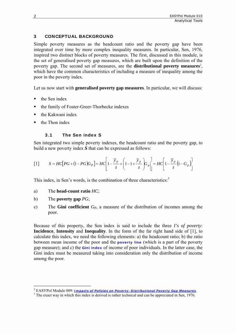
Simple poverty measures as the headcount ratio and the poverty gap have been integrated over time by more complex inequality measures. In particular, Sen, 1976, inspired two distinct blocks of poverty measures. The first, discussed in this module, is the set of generalised poverty gap measures, which are built upon the definition of the poverty gap. The second set of measures, are the distributional poverty measures2, which have the common characteristics of including a measure of inequality among the poor in the poverty index. Let us now start with generalised poverty gap measures. In particular, we will discuss: the Sen index

the family of Foster-Greer-Thorbecke indexes

the Kakwani index

the Thon index

3.1 The Sen index S

Sen integrated two simple poverty indexes, the headcount ratio and the poverty gap, to build a new poverty index S that can be expressed as follows:

[1] ( )[ ] ( )⎥⎦

⎤⎢⎣

⎡−−=

⎥⎥⎦

⎤

⎢⎢⎣

⎡⎟⎟⎠

⎞⎜⎜⎝

⎛+−+−=−+= p

pp

ppP G

zy

HCGz

yz

yHCGPGPGHCS 111111

This index, in Sen’s words, is the combination of three characteristics:3

a) The head-count ratio HC;

b) The poverty gap PG;

c) The Gini coefficient GP, a measure of the distribution of incomes among the poor.

Because of this property, the Sen index is said to include the three I’s of poverty: Incidence, Intensity and Inequality. In the form of the far right hand side of [1], to calculate this index, we need the following elements: a) the headcount ratio; b) the ratio between mean income of the poor and the poverty line (which is a part of the poverty gap measure); and c) the Gini index of income of poor individuals. In the latter case, the Gini index must be measured taking into consideration only the distribution of income among the poor.

2 EASYPol Module 009: Impacts of Policies on Poverty: Distributional Poverty Gap Measures. 3 The exact way in which this index is derived is rather technical and can be appreciated in Sen, 1976.



http://www.fao.org/docs/up/easypol/322/distributional-pvmsrs_009EN.pdf


3

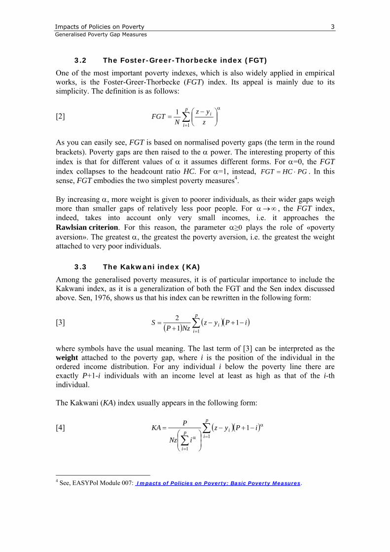
3.2 The Foster-Greer-Thorbecke index (FGT)

One of the most important poverty indexes, which is also widely applied in empirical works, is the Foster-Greer-Thorbecke (FGT) index. Its appeal is mainly due to its simplicity. The definition is as follows:

[2] ∑=

α

⎟⎟⎠

⎞⎜⎜⎝

⎛ −=

p

i

i

zyz

NFGT

1

1

As you can easily see, FGT is based on normalised poverty gaps (the term in the round brackets). Poverty gaps are then raised to the α power. The interesting property of this index is that for different values of α it assumes different forms. For α=0, the FGT index collapses to the headcount ratio HC. For α=1, instead, . In this sense, FGT embodies the two simplest poverty measures

PGHCFGT ⋅=4.

By increasing α, more weight is given to poorer individuals, as their wider gaps weigh more than smaller gaps of relatively less poor people. For ∞→α , the FGT index, indeed, takes into account only very small incomes, i.e. it approaches the Rawlsian criterion. For this reason, the parameter α≥0 plays the role of «poverty aversion». The greatest α, the greatest the poverty aversion, i.e. the greatest the weight attached to very poor individuals.

3.3 The Kakwani index (KA)

Among the generalised poverty measures, it is of particular importance to include the Kakwani index, as it is a generalization of both the FGT and the Sen index discussed above. Sen, 1976, shows us that his index can be rewritten in the following form:

[3] ( ) ( )(∑=

−+−+

=p

ii iPyz

NzPS

11

12 )

where symbols have the usual meaning. The last term of [3] can be interpreted as the weight attached to the poverty gap, where i is the position of the individual in the ordered income distribution. For any individual i below the poverty line there are exactly P+1-i individuals with an income level at least as high as that of the i-th individual. The Kakwani (KA) index usually appears in the following form:

[4] ( )( )∑∑ =

α

=

α

−+−

⎟⎟⎠

⎞⎜⎜⎝

⎛=

p

iip

i

iPyz

iNz

PKA1

1

1

4 See, EASYPol Module 007: Impacts of Policies on Poverty: Basic Poverty Measures.

http://www.fao.org/docs/up/easypol/323/basic-pov-measures_007EN.pdf


4

The meaning of the α-power, as in the case of the FGT index, is to give relatively more weight to poorer people. When an individual is extremely poor, (P+1-i) is larger. For example, if one individual is the poorest out of twenty poor people, i will be equal to 1 and the weight will be equal to 20. Raising large numbers gives proportionally higher numbers than raising small numbers, so that the poverty gap of poorest individuals gets more weight. KA collapses to the Sen index under the hypothesis α=1. This is easily seen by observing that for α=1 the round bracket at the denominator of [4] is equal to (P+1)(P/2). When α=0, KA collapses to the FGT with α=1, as in this case

PGHCzP

yzNPKA

p

i

i ⋅=⎟⎠

⎞⎜⎝

⎛ −= ∑

=1. For empirical applications, therefore, the use of the

Kakwani index is meaningful if α>1.

3.4 The Thon index (TH)

The Thon index follows the same logic as the Kakwani index. In this sense it is also derived from the Sen index. The main difference is that the weight of the poverty gap is here measured considering the total number of individuals and not just the number of poor individuals. In other words, instead of having (P+1-i), the Thon index assumes (N+1-i). Normalising this index we can yield:

[5] ( )( iNyzNzN

THi

i −+−+

= ∑ 1)1(

2 )

where symbols have the usual meaning. The main difference with the Sen index, in version [3], is that the Thon index considers the total number of individuals N rather than the number of poor individuals P.

4 A STEP-BY-STEP PROCEDURE TO CALCULATE GENERALISED POVERTY GAP MEASURES

4.1 A step-by-step procedure to calculate S

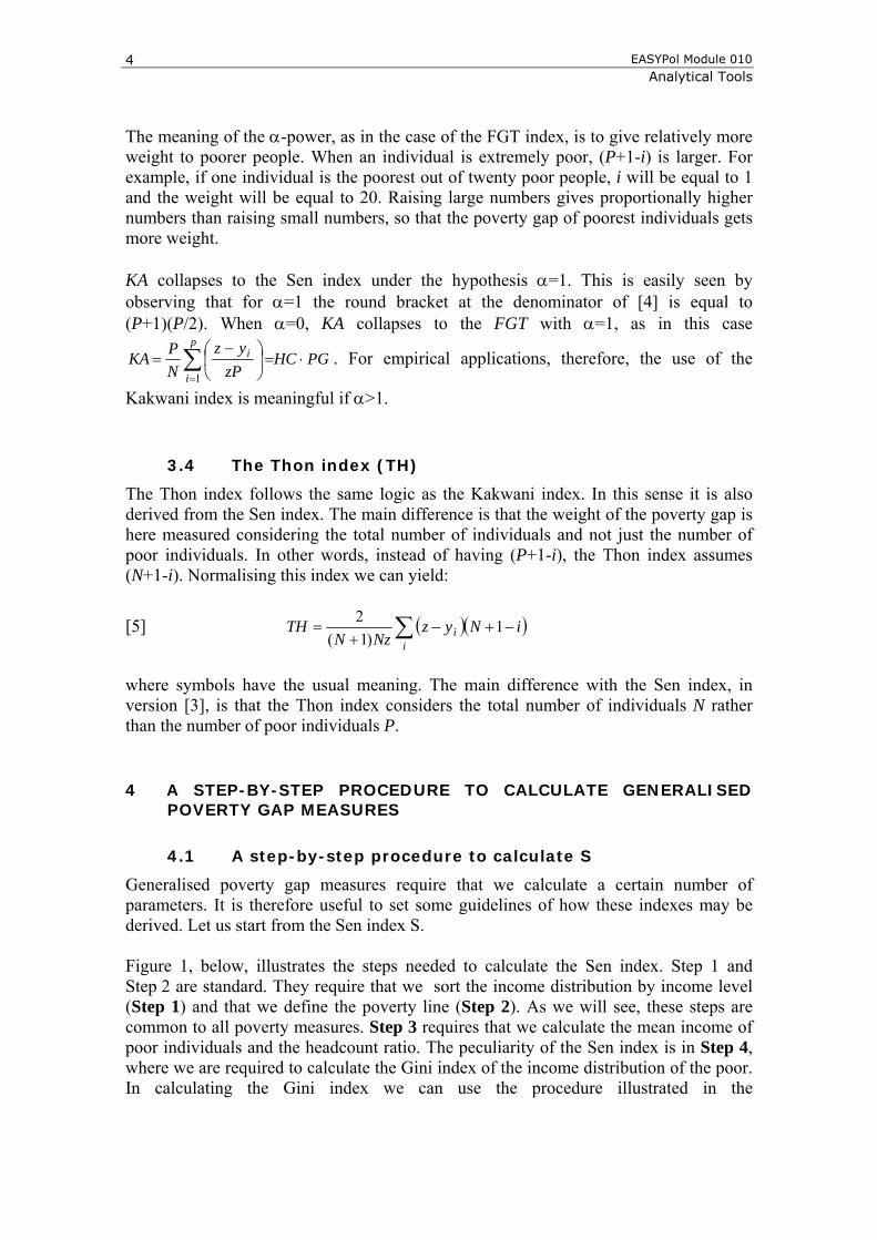
Generalised poverty gap measures require that we calculate a certain number of parameters. It is therefore useful to set some guidelines of how these indexes may be derived. Let us start from the Sen index S. Figure 1, below, illustrates the steps needed to calculate the Sen index. Step 1 and Step 2 are standard. They require that we sort the income distribution by income level (Step 1) and that we define the poverty line (Step 2). As we will see, these steps are common to all poverty measures. Step 3 requires that we calculate the mean income of poor individuals and the headcount ratio. The peculiarity of the Sen index is in Step 4, where we are required to calculate the Gini index of the income distribution of the poor. In calculating the Gini index we can use the procedure illustrated in the


5

EASYPol module for inequality measurement5, by taking into account that, in this case, only income of poor individuals must be considered. After having calculated the Gini index of the poor, the Sen index can be easily calculated by applying formula [1] (Step 5).

Figure 1 - A step-by-step procedure to calculate S

STEP Operational content

1If not already sorted, sort the income distribution by income

level

2 Define the poverty line

3Calculate the mean income of

poor individuals and the headcount ratio

4Calculate the Gini index of income of poor individuals

5Calculate the SEN index by

applying formula [1]

4.2 A step-by-step procedure to calculate FGT

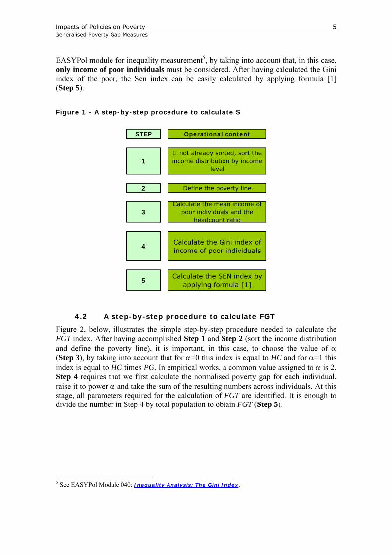
Figure 2, below, illustrates the simple step-by-step procedure needed to calculate the FGT index. After having accomplished Step 1 and Step 2 (sort the income distribution and define the poverty line), it is important, in this case, to choose the value of α (Step 3), by taking into account that for α=0 this index is equal to HC and for α=1 this index is equal to HC times PG. In empirical works, a common value assigned to α is 2. Step 4 requires that we first calculate the normalised poverty gap for each individual, raise it to power α and take the sum of the resulting numbers across individuals. At this stage, all parameters required for the calculation of FGT are identified. It is enough to divide the number in Step 4 by total population to obtain FGT (Step 5).

5 See EASYPol Module 040: Inequality Analysis: The Gini Index.

http://www.fao.org/docs/up/easypol/329/gini_index_040EN.pdf


6

Figure 2 - A step-by-step procedure to calculate FGT


1If not already sorted, sort the income

distribution by income level


3 Choose the level of α.

4

For poor people, define the difference between the poverty line and their

individual incomes. Then divide the result by the poverty line. Raise the result to

power α and take the sum

5 Calculate FGT by applying formula [2]

4.3 A step-by-step procedure to calculate KA

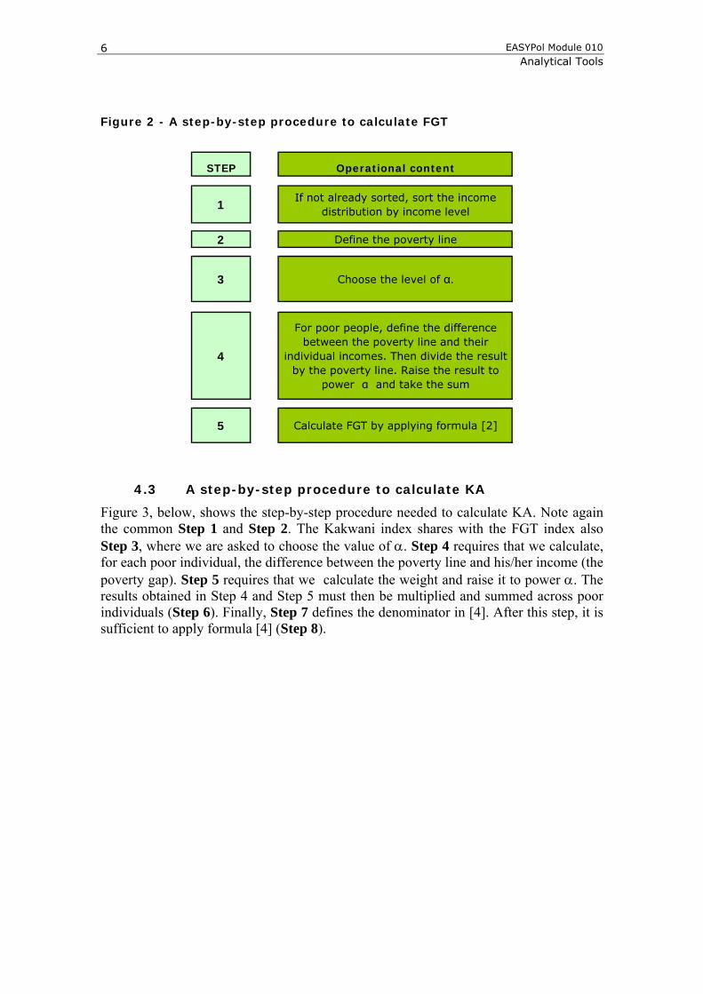
Figure 3, below, shows the step-by-step procedure needed to calculate KA. Note again the common Step 1 and Step 2. The Kakwani index shares with the FGT index also Step 3, where we are asked to choose the value of α. Step 4 requires that we calculate, for each poor individual, the difference between the poverty line and his/her income (the poverty gap). Step 5 requires that we calculate the weight and raise it to power α. The results obtained in Step 4 and Step 5 must then be multiplied and summed across poor individuals (Step 6). Finally, Step 7 defines the denominator in [4]. After this step, it is sufficient to apply formula [4] (Step 8).


7

Figure 3 - A step-by-step procedure to calculate KA


1If not already sorted, sort the income

distribution by income level


3 Choose the level of α

4For poor people, define the difference

between the poverty line and each income

5 Define the value (P+1-1)α

6Multiply values in Steps 4 and 5 and take

the sum

7 Define Iα and take the sum

8 Calculate KA by applying formula [4]

4.4 A step-by-step procedure to calculate TH

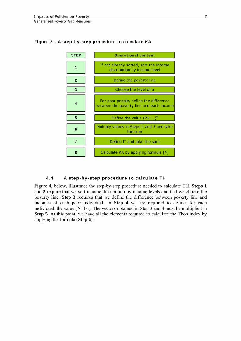
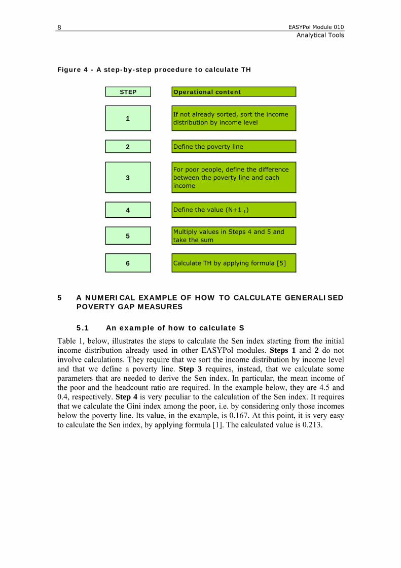
Figure 4, below, illustrates the step-by-step procedure needed to calculate TH. Steps 1 and 2 require that we sort income distribution by income levels and that we choose the poverty line. Step 3 requires that we define the difference between poverty line and incomes of each poor individual. In Step 4 we are required to define, for each individual, the value (N+1-i). The vectors obtained in Step 3 and 4 must be multiplied in Step 5. At this point, we have all the elements required to calculate the Thon index by applying the formula (Step 6).


8

Figure 4 - A step-by-step procedure to calculate TH


1If not already sorted, sort the income distribution by income level


3For poor people, define the difference between the poverty line and each income

4 Define the value (N+1-1)

5Multiply values in Steps 4 and 5 and take the sum

6 Calculate TH by applying formula [5]

5 A NUMERICAL EXAMPLE OF HOW TO CALCULATE GENERALISED POVERTY GAP MEASURES

5.1 An example of how to calculate S

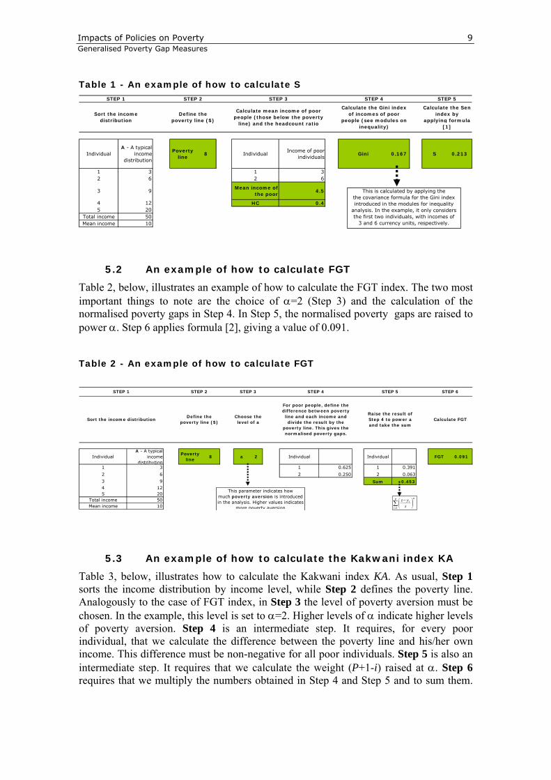
Table 1, below, illustrates the steps to calculate the Sen index starting from the initial income distribution already used in other EASYPol modules. Steps 1 and 2 do not involve calculations. They require that we sort the income distribution by income level and that we define a poverty line. Step 3 requires, instead, that we calculate some parameters that are needed to derive the Sen index. In particular, the mean income of the poor and the headcount ratio are required. In the example below, they are 4.5 and 0.4, respectively. Step 4 is very peculiar to the calculation of the Sen index. It requires that we calculate the Gini index among the poor, i.e. by considering only those incomes below the poverty line. Its value, in the example, is 0.167. At this point, it is very easy to calculate the Sen index, by applying formula [1]. The calculated value is 0.213.


9

Table 1 - An example of how to calculate S

Individual A - A typical

incomedistribution

Poverty line

8 Individual Income of poor

individualsGini 0.167 S 0.213

1 3 1 32 6 2 6

3 9Mean income of

the poor4.5

4 12 HC 0.45 20

Total income 50Mean income 10

STEP 5

Calculate the Sen index by

applying formula [1]

Sort the income distribution

Define the poverty line ($)

Calculate mean income of poor people (those below the poverty

line) and the headcount ratio

Calculate the Gini index of incomes of poor

people (see modules on inequality)

STEP 1 STEP 2 STEP 3 STEP 4

This is calculated by applying the the covariance formula for the Gini indexintroduced in the modules for inequality

analysis. In the example, it only considersthe first two individuals, with incomes of

3 and 6 currency units, respectively.

5.2 An example of how to calculate FGT

Table 2, below, illustrates an example of how to calculate the FGT index. The two most important things to note are the choice of α=2 (Step 3) and the calculation of the normalised poverty gaps in Step 4. In Step 5, the normalised poverty gaps are raised to power α. Step 6 applies formula [2], giving a value of 0.091.

Table 2 - An example of how to calculate FGT


incomedistribution

Poverty line

8 a 2 Individual Individual FGT 0.091

1 3 1 0.625 1 0.391

2 6 2 0.250 2 0.063

3 9 Sum 0.4534 125 20


Calculate FGTSort the income distributionDefine the

poverty line ($)Choose the level of a

For poor people, define the difference between poverty line and each income and divide the result by the

poverty line. This gives the normalised poverty gaps.

Raise the result of Step 4 to power a and take the sum

STEP 6STEP 1 STEP 2 STEP 3 STEP 4 STEP 5

This parameter indicates howmuch poverty aversion is introducedin the analysis. Higher values indicates

more poverty aversion∑=

α

⎟⎟⎠

⎞⎜⎜⎝

⎛ −p

i

i

zyz

1

5.3 An example of how to calculate the Kakwani index KA

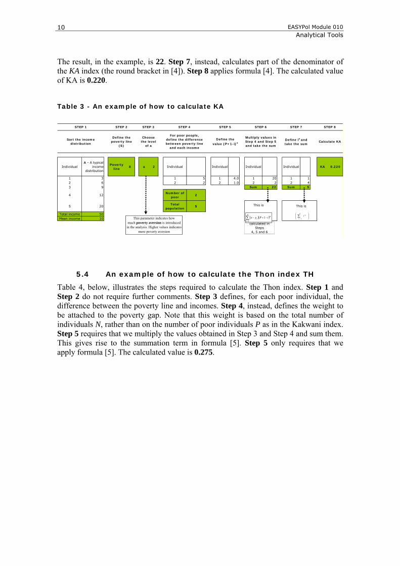
Table 3, below, illustrates how to calculate the Kakwani index KA. As usual, Step 1 sorts the income distribution by income level, while Step 2 defines the poverty line. Analogously to the case of FGT index, in Step 3 the level of poverty aversion must be chosen. In the example, this level is set to α=2. Higher levels of α indicate higher levels of poverty aversion. Step 4 is an intermediate step. It requires, for every poor individual, that we calculate the difference between the poverty line and his/her own income. This difference must be non-negative for all poor individuals. Step 5 is also an intermediate step. It requires that we calculate the weight (P+1-i) raised at α. Step 6 requires that we multiply the numbers obtained in Step 4 and Step 5 and to sum them.


10

The result, in the example, is 22. Step 7, instead, calculates part of the denominator of the KA index (the round bracket in [4]). Step 8 applies formula [4]. The calculated value of KA is 0.220.

Table 3 - An example of how to calculate KA


incomedistribution

Poverty line

8 a 2 Individual Individual Individual Individual KA 0.220

1 3 1 5 1 4.0 1 20 1 12 6 2 2 2 1.0 2 2 2 43 9 Sum 22 Sum 5

4 12Number of

poor2

5 20Total

population5


STEP 1 STEP 2 STEP 4 STEP 5STEP 3

Sort the income distribution

Define the poverty line

($)

For poor people, define the difference between poverty line

and each income

Define the value (P+1-i)a

Choose the level

of a

STEP 8

Calculate KA

STEP 6

Multiply values in Step 4 and Step 5 and take the sum

STEP 7

Define ia and take the sum

This parameter indicates howmuch poverty aversion is introduced

in the analysis. Higher values indicatesmore poverty aversion

⎟⎟⎠

⎞⎜⎜⎝

⎛∑=

αp

ii

1

This isThis is

( )( )∑=

α−+−p

ii iPyz

11

calculated in Steps

4, 5 and 6

5.4 An example of how to calculate the Thon index TH

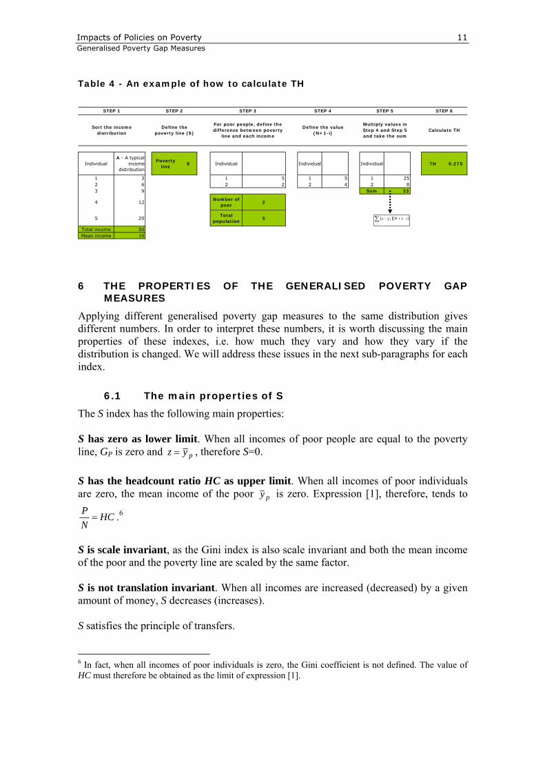
Table 4, below, illustrates the steps required to calculate the Thon index. Step 1 and Step 2 do not require further comments. Step 3 defines, for each poor individual, the difference between the poverty line and incomes. Step 4, instead, defines the weight to be attached to the poverty gap. Note that this weight is based on the total number of individuals N, rather than on the number of poor individuals P as in the Kakwani index. Step 5 requires that we multiply the values obtained in Step 3 and Step 4 and sum them. This gives rise to the summation term in formula [5]. Step 5 only requires that we apply formula [5]. The calculated value is 0.275.


11

Table 4 - An example of how to calculate TH


incomedistribution

Poverty line

8 Individual Individual Individual TH 0.275

1 3 1 5 1 5 1 252 6 2 2 2 4 2 83 9 Sum 33

4 12Number of

poor2

5 20Total

population5


STEP 4 STEP 5 STEP 6STEP 1 STEP 2 STEP 3

Define the value (N+1-i)

Multiply values in Step 4 and Step 5 and take the sum

Calculate THSort the income

distributionDefine the

poverty line ($)

For poor people, define the difference between poverty

line and each income

( )( )iNyzi

i −+−∑ 1

6 THE PROPERTIES OF THE GENERALISED POVERTY GAP MEASURES

Applying different generalised poverty gap measures to the same distribution gives different numbers. In order to interpret these numbers, it is worth discussing the main properties of these indexes, i.e. how much they vary and how they vary if the distribution is changed. We will address these issues in the next sub-paragraphs for each index.

6.1 The main properties of S

The S index has the following main properties: S has zero as lower limit. When all incomes of poor people are equal to the poverty line, GP is zero and pyz = , therefore S=0. S has the headcount ratio HC as upper limit. When all incomes of poor individuals are zero, the mean income of the poor py is zero. Expression [1], therefore, tends to

HCNP= .6

S is scale invariant, as the Gini index is also scale invariant and both the mean income of the poor and the poverty line are scaled by the same factor. S is not translation invariant. When all incomes are increased (decreased) by a given amount of money, S decreases (increases). S satisfies the principle of transfers. 6 In fact, when all incomes of poor individuals is zero, the Gini coefficient is not defined. The value of HC must therefore be obtained as the limit of expression [1].


12

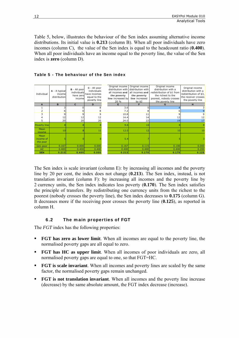
Table 5, below, illustrates the behaviour of the Sen index assuming alternative income distributions. Its initial value is 0.213 (column B). When all poor individuals have zero incomes (column C), the value of the Sen index is equal to the headcount ratio (0.400). When all poor individuals have an income equal to the poverty line, the value of the Sen index is zero (column D).

Table 5 - The behaviour of the Sen index


incomedistribution

B - All poorindividualshave zero

income

C - All poorindividuals

have incomesequal to thepoverty line

Original income distribution with all incomes and

the poverty line increased by

20 %


the poverty line increased

by $2

Original income distribution with a

redistribution of $1 from the richest to the

poorest, nobody crosses the poverty line


redistribution of $3,the receiver crosses

the poverty line

A B C D E F G H1 3 0 8 3.6 5 42 6 0 8 7.2 8 63 9 9 9 10.8 11 94 12 12 12 14.4 14 125 20 20 20 24.0 22 19

Poverty line 8 8 8 9.6 10 8 8

Mean income

10 8 11 12.0 12 10 10

Mean income of the poor

5 0 8 5.4 7 5

Gini poor 0.167 0.000 0.000 0.167 0.115 0.100 0.000HC 0.400 0.400 0.400 0.400 0.400 0.400 0.200

SEN 0.213 0.400 0.000 0.213 0.170 0.175 0.125

399

1217

3

The Sen index is scale invariant (column E): by increasing all incomes and the poverty line by 20 per cent, the index does not change (0.213). The Sen index, instead, is not translation invariant (column F): by increasing all incomes and the poverty line by 2 currency units, the Sen index indicates less poverty (0.170). The Sen index satisfies the principle of transfers. By redistributing one currency units from the richest to the poorest (nobody crosses the poverty line), the Sen index decreases to 0.175 (column G). It decreases more if the receiving poor crosses the poverty line (0.125), as reported in column H.

6.2 The main properties of FGT

The FGT index has the following properties: FGT has zero as lower limit. When all incomes are equal to the poverty line, the

normalised poverty gaps are all equal to zero.

FGT has HC as upper limit. When all incomes of poor individuals are zero, all normalised poverty gaps are equal to one, so that FGT=HC.

FGT is scale invariant. When all incomes and poverty lines are scaled by the same factor, the normalised poverty gaps remain unchanged.

FGT is not translation invariant. When all incomes and the poverty line increase (decrease) by the same absolute amount, the FGT index decrease (increase).


13

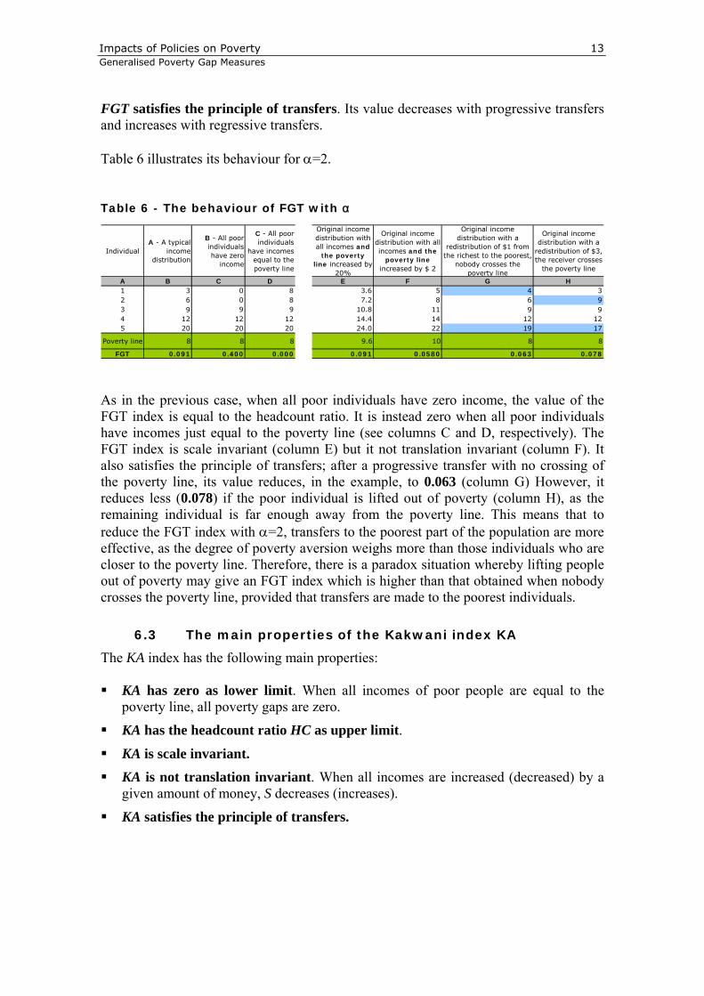
FGT satisfies the principle of transfers. Its value decreases with progressive transfers and increases with regressive transfers. Table 6 illustrates its behaviour for α=2.

Table 6 - The behaviour of FGT with α


incomedistribution


income




the poverty line increased by

20%

Original income distribution with allincomes and the

poverty line increased by $ 2


redistribution of $1 from the richest to the poorest,

nobody crosses the poverty line



the poverty line

A B C D E F G H1 3 0 8 3.6 5 42 6 0 8 7.2 8 63 9 9 9 10.8 11 9 94 12 12 12 14.4 14 12 125 20 20 20 24.0 22 19 17

Poverty line 8 8 8 9.6 10 8 8

FGT 0.091 0.400 0.000 0.091 0.0580 0.063 0.078

39

As in the previous case, when all poor individuals have zero income, the value of the FGT index is equal to the headcount ratio. It is instead zero when all poor individuals have incomes just equal to the poverty line (see columns C and D, respectively). The FGT index is scale invariant (column E) but it not translation invariant (column F). It also satisfies the principle of transfers; after a progressive transfer with no crossing of the poverty line, its value reduces, in the example, to 0.063 (column G) However, it reduces less (0.078) if the poor individual is lifted out of poverty (column H), as the remaining individual is far enough away from the poverty line. This means that to reduce the FGT index with α=2, transfers to the poorest part of the population are more effective, as the degree of poverty aversion weighs more than those individuals who are closer to the poverty line. Therefore, there is a paradox situation whereby lifting people out of poverty may give an FGT index which is higher than that obtained when nobody crosses the poverty line, provided that transfers are made to the poorest individuals.

6.3 The main properties of the Kakwani index KA

The KA index has the following main properties: KA has zero as lower limit. When all incomes of poor people are equal to the

poverty line, all poverty gaps are zero.

KA has the headcount ratio HC as upper limit.

KA is scale invariant.

KA is not translation invariant. When all incomes are increased (decreased) by a given amount of money, S decreases (increases).

KA satisfies the principle of transfers.


14

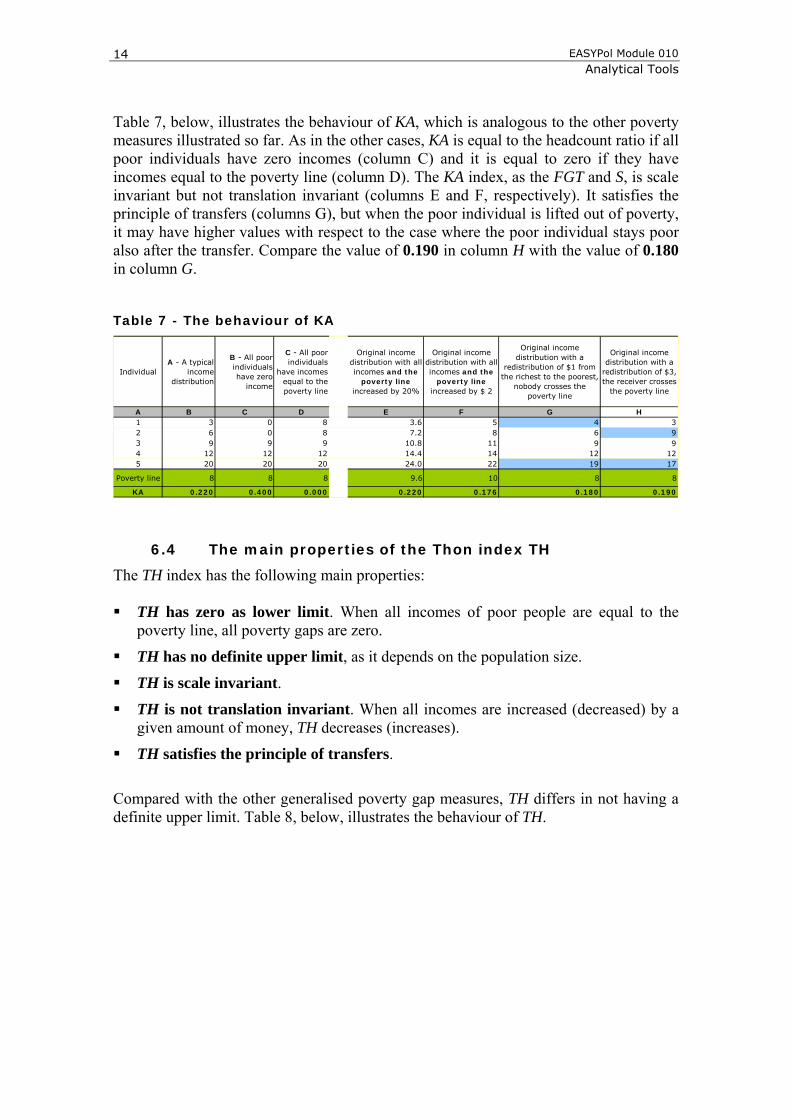
Table 7, below, illustrates the behaviour of KA, which is analogous to the other poverty measures illustrated so far. As in the other cases, KA is equal to the headcount ratio if all poor individuals have zero incomes (column C) and it is equal to zero if they have incomes equal to the poverty line (column D). The KA index, as the FGT and S, is scale invariant but not translation invariant (columns E and F, respectively). It satisfies the principle of transfers (columns G), but when the poor individual is lifted out of poverty, it may have higher values with respect to the case where the poor individual stays poor also after the transfer. Compare the value of 0.190 in column H with the value of 0.180 in column G.

Table 7 - The behaviour of KA


incomedistribution


income



Original income distribution with all incomes and the

poverty line increased by 20%

Original income distribution with allincomes and the

poverty line increased by $ 2


redistribution of $1 from the richest to the poorest,

nobody crosses the poverty line



the poverty line

A B C D E F G H1 3 0 8 3.6 5 42 6 0 8 7.2 8 63 9 9 9 10.8 11 9 94 12 12 12 14.4 14 12 125 20 20 20 24.0 22 19 17

Poverty line 8 8 8 9.6 10 8 8

KA 0.220 0.400 0.000 0.220 0.176 0.180 0.190

39

6.4 The main properties of the Thon index TH

The TH index has the following main properties: TH has zero as lower limit. When all incomes of poor people are equal to the

poverty line, all poverty gaps are zero.

TH has no definite upper limit, as it depends on the population size.

TH is scale invariant.

TH is not translation invariant. When all incomes are increased (decreased) by a given amount of money, TH decreases (increases).

TH satisfies the principle of transfers.

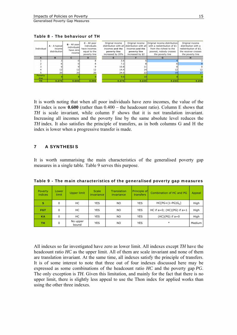
Compared with the other generalised poverty gap measures, TH differs in not having a definite upper limit. Table 8, below, illustrates the behaviour of TH.


15

Table 8 - The behaviour of TH


incomedistribution


income




poverty line increased by 20%


poverty line increased by $2

Original income distribution with a redistribution of $1

from the richest to the poorest, nobody crosses

the poverty line


redistribution of $3, the receiver crosses

the poverty line

A B C D E F G H1 3 0 8 3.6 5 42 6 0 8 7.2 8 63 9 9 9 10.8 11 9 94 12 12 12 14.4 14 125 20 20 20 24.0 22 19

Povert

39

1217

y line

8 8 8 9.6 10 8

TH 0.275 0.600 0.000 0.275 0.220 0.233 0.208

8

It is worth noting that when all poor individuals have zero incomes, the value of the TH index is now 0.600 (rather than 0.400 – the headcount ratio). Column E shows that TH is scale invariant, while column F shows that it is not translation invariant. Increasing all incomes and the poverty line by the same absolute level reduces the TH index. It also satisfies the principle of transfers, as in both columns G and H the index is lower when a progressive transfer is made.

7 A SYNTHESIS

It is worth summarising the main characteristics of the generalised poverty gap measures in a single table. Table 9 serves this purpose.

Table 9 - The main characteristics of the generalised poverty gap measures

Poverty indices

Lower limit

Upper limitScale

invarianceTranslation invariance

Principle oftransfers

Combination of HC and PG Appeal

S 0 HC YES NO YES HC[PG+(1-PG)Gp] High

FGT 0 HC YES NO YES HC if a=0; (HC)(PG) if a=1 High

KA 0 HC YES NO YES (HC)(PG) if a=0 High

TH 0No upper

boundYES NO YES * Medium

All indexes so far investigated have zero as lower limit. All indexes except TH have the headcount ratio HC as the upper limit. All of them are scale invariant and none of them are translation invariant. At the same time, all indexes satisfy the principle of transfers. It is of some interest to note that three out of four indexes discussed here may be expressed as some combinations of the headcount ratio HC and the poverty gap PG. The only exception is TH. Given this limitation, and mainly for the fact that there is no upper limit, there is slightly less appeal to use the Thon index for applied works than using the other three indexes.


16

8 READERS’ NOTES

8.1 Time requirements

The delivery of this module to an audience already familiar with the definition of poverty both in absolute and relative terms and with the simplest ways to define poverty may take about three hours.

8.2 Frequently asked questions

How do I select among many poverty indexes? There is no clear-cut answer to this question. The choice of the poverty index may depend on the type of analysis that is carried out. A good guide to select among indexes, however, is to know how they react to changes in the income distribution (axioms).

Is it possible that different poverty indexes give different answers? Yes, it is. Since different poverty indexes react differently to shocks in the income distribution, the possibility of having contradictory results must be taken into account. This is the reason why different poverty indexes should be calculated in applied works.

What is the advantage of using generalised poverty gap measures? There is no definite advantage of using these indexes compared with other classes of poverty measures. However, they share the nice feature of being based on a readily interpretable poverty measure, i.e., the poverty gap. Many of them are also useful combinations of the poverty gap and of the headcount ratio.

8.3 Complementary capacity building materials

Complementary EASYPol modules are: EASYPol Module 004: Impacts of Policies on Poverty: The Definition of Poverty EASYPol Module 005: Impacts of Policies on Poverty: Absolute Poverty Lines

EASYPol Module 006: Impacts of Policies on Poverty: Relative Poverty Lines EASYPol Module 009: Impacts of Polcies on Poverty: Distributional Poverty Gap

Measures EASYPol Module 035: Impacts of Policies on Poverty: Poverty and Dominance

9 REFERENCES AND FURTHER READINGS

Deaton A., 1997. The Analysis of Household Surveys, The Johns Hopkins University

Press, Baltimore, USA. Foster J., Greer J., Thorbecke E., 1984. A Class of Decomposable Poverty Measures,

Econometrica, 52, pp. 761-766. Kakwani N., 1980. On A Class of Poverty Measures, Econometrica, 48, pp. 431-436.

http://www.fao.org/docs/up/easypol/312/povanlys_defpov_004EN.pdf

http://www.fao.org/docs/up/easypol/316/abslt_pov_lines_005EN.pdf

http://www.fao.org/docs/up/easypol/317/rel_pov_lines_006EN.pdf



http://www.fao.org/docs/up/easypol/328/povety&dominance_035EN.pdf


17

Lambert P., 2001. The Distribution and Redistribution of Income, Manchester University Press, Manchester, UK, 3rd edition.

Sen A., 1976. Poverty: An Ordinal Approach to Measurement, Econometrica, 44. Sen A., 1997. On Economic Inequality, Clarendon Press, Oxford, UK. Thon D., 1979. On Measuring Poverty, Review of Income and Wealth, 25, pp. 429-439.


18

Module metadata

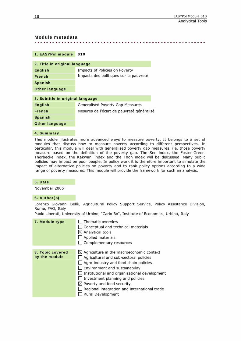
1. EASYPol module 010

2. Title in original language

English Impacts of Policies on Poverty

French Impacts des politiques sur la pauvreté

Spanish

Other language

3. Subtitle in original language

English Generalised Poverty Gap Measures

French Mesures de l’écart de pauvreté généralisé

Spanish

Other language

4. Summary

This module illustrates more advanced ways to measure poverty. It belongs to a set of modules that discuss how to measure poverty according to different perspectives. In particular, this module will deal with generalised poverty gap measures, i.e. those poverty measure based on the definition of the poverty gap. The Sen index, the Foster-Greer-Thorbecke index, the Kakwani index and the Thon index will be discussed. Many public policies may impact on poor people. In policy work it is therefore important to simulate the impact of alternative policies on poverty and to rank policy options according to a wide range of poverty measures. This module will provide the framework for such an analysis.

5. Date

November 2005

6. Author(s)

Lorenzo Giovanni Bellù, Agricultural Policy Support Service, Policy Assistance Division, Rome, FAO, Italy Paolo Liberati, University of Urbino, "Carlo Bo", Institute of Economics, Urbino, Italy

7. Module type

Thematic overview Conceptual and technical materials Analytical tools Applied materials Complementary resources

8. Topic covered by the module

Agriculture in the macroeconomic context Agricultural and sub-sectoral policies Agro-industry and food chain policies Environment and sustainability Institutional and organizational development Investment planning and policies Poverty and food security Regional integration and international trade Rural Development


19

9. Subtopics covered by the module

10. Training path Analysis and monitoring of socio-economic impacts of policies

11. Keywords

Impacts of Policies on Poverty : Generalised Poverty Gap ...

Documents

Transcript of Impacts of Policies on Poverty : Generalised Poverty Gap ...