UNIVERSIDADE FEDERAL DO RIO GRANDE DO SULINSTITUTO DE INFORMÁTICA

PROGRAMA DE PÓS-GRADUAÇÃO EM COMPUTAÇÃO

GIOVANE ROSLINDO KUHN

Image Recoloring forColor-Vision Deficients

Thesis presented in partial fulfillmentof the requirements for the degree ofMaster of Computer Science

Prof. Dr. Manuel Menezes de Oliveira NetoAdvisor

Porto Alegre, April 2008

CIP – CATALOGING-IN-PUBLICATION

Kuhn, Giovane Roslindo

Image Recoloring forColor-Vision Deficients / Giovane Roslindo Kuhn. – Porto Ale-gre: PPGC da UFRGS, 2008.

61 f.: il.

Thesis (Master) – Universidade Federal do Rio Grande do Sul.Programa de Pós-Graduação em Computação, Porto Alegre, BR–RS, 2008. Advisor: Manuel Menezes de Oliveira Neto.

1. Color Reduction, Color-Contrast Enhancement, Color-to-Grayscale Mapping, Color Vision Deficiency, Dichromacy, Er-ror Metric, Image Processing, Monochromacy, Recoloring Algo-rithm. I. Oliveira Neto, Manuel Menezes de. II. Title.

UNIVERSIDADE FEDERAL DO RIO GRANDE DO SULReitor: Prof. José Carlos Ferraz HennemannVice-Reitor: Prof. Pedro Cezar Dutra FonsecaPró-Reitora de Pós-Graduação: Profa. Valquíria Linck BassaniDiretor do Instituto de Informática: Prof. Flávio Rech WagnerCoordenadora do PPGC: Profa. Luciana Porcher NedelBibliotecária-Chefe do Instituto de Informática: BeatrizRegina Bastos Haro

“Knowledge becomes knowledge, when it’s in the mind of everyone.”— ANONYMOUS

ACKNOWLEDGMENTS

I dedicate this work to two people in particular: Roberta Magalhães, my faithful com-panion, even in the distance gave me all your love and comprehension, fundamental thatI do not give up the master’s program, make my bags and get backhome. Edir RoslindoKuhn, my dear mother, for her thirst for life and strength in difficult moments, whichspread me and keep moving forward.

I thank immensely my advisor Manuel Menezes de Oliveira Neto, even with his post-abolitionist method, he always took me to my limit and made megrow professionallyin a unprecedented way in my life. I thank him for the various conversations about hisexperience both in professional and private life, which certainly were a learning processfor me. I would also like to thank for his style of work, which always yielded the bestjokes in the labs and conversations at parties.

I would like to thank Flavio Brum, a dichromat who was the great inspiration forthe development of this work and responsible for valuable priceless suggestions. I thankSandro Fiorini, an anomalous trichromat, for the various testimonies of the difficultiesfaced by him on daily tasks. I am grateful to Carlos Dietrich for the discussions aboutmass-spring systems and for the base code to solvers on the CPU and GPU. I thank Ed-uardo Pons by illustrations developed for this work and for the papers submitted, BárbaraBellaver for the provision in the development of videos to the papers of this work, Le-andro Fernandes by the partnership in the submission of one of the papers, and AndréSpritzer by English revisions.

I thank the professors Carla Freitas, João Comba, Luciana Nedel and Manuel Oliveirafor their mastery in leading the Computer Graphics Group at UFRGS, and for their will-ingness to assist the students in the program. Thanks to professors Paulo Rodacki, JomiHübner and Dalton Solano dos Reis, from the Regional University of Blumenau (FURB),for the letters of recommendation. I also thank my colleagues in the Computer GraphicsGroup, that always propitiated a creative and relaxed environment in the labs, importantfor the development of this work and my intellectual growth.

Thanks to my parents José Cildo Kuhn and Edir Roslindo Kuhn for my educationand freedom of choice, my brothers Giselle Roslindo Kuhn andVitor Roslindo Kuhn byaffection even in the distance, and my family and all friendswho understood my absencein the last festive events. I also thank my neighbor Márcia Moares and her family, withall the fundamental support and friendship during my stay inPorto Alegre. Thanks toTriangle Fans, the best soccer team in the world, okay, in theCG world at UFRGS, forthe glorious moments in the field, and I also thank Polar beer that always refreshed mymoments in Porto Alegre.

I thank CAPES Brazil by partial financial support for this work and a special thanksto my friend Vitor Pamplona for financial help throughout my stay in Porto Alegre.

TABLE OF CONTENTS

LIST OF FIGURES . . . . . . . . . . . . . . . . . . . . . . . . . . . . . . . . 9

LIST OF TABLES . . . . . . . . . . . . . . . . . . . . . . . . . . . . . . . . 11

ABSTRACT . . . . . . . . . . . . . . . . . . . . . . . . . . . . . . . . . . . 13

RESUMO . . . . . . . . . . . . . . . . . . . . . . . . . . . . . . . . . . . . . 15

1 INTRODUCTION . . . . . . . . . . . . . . . . . . . . . . . . . . . . . . 171.1 Thesis Contributions . . . . . . . . . . . . . . . . . . . . . . . . . . . . . 201.2 Structure of the Thesis . . . . . . . . . . . . . . . . . . . . . . . . . . . . 20

2 RELATED WORK . . . . . . . . . . . . . . . . . . . . . . . . . . . . . . 212.1 Simulation of Dichromat’s Perception . . . . . . . . . . . . . . . . . . . 212.2 Recoloring Techniques for Dichromats. . . . . . . . . . . . . . . . . . . 222.2.1 User-Assisted Recoloring Techniques . . . . . . . . . . . . .. . . . . . 222.2.2 Automatic Recoloring Techniques . . . . . . . . . . . . . . . . .. . . . 232.3 Color-to-Grayscale Techniques . . . . . . . . . . . . . . . . . . . . . . . 242.4 Summary . . . . . . . . . . . . . . . . . . . . . . . . . . . . . . . . . . . 26

3 MASS-SPRING SYSTEMS . . . . . . . . . . . . . . . . . . . . . . . . . 293.1 Definition of Mass-Spring Systems . . . . . . . . . . . . . . . . . . . . . 293.2 Dynamic of Mass-Spring Systems. . . . . . . . . . . . . . . . . . . . . . 303.3 Summary . . . . . . . . . . . . . . . . . . . . . . . . . . . . . . . . . . . 31

4 THE RECOLORING ALGORITHM FOR DICHROMATS . . . . . . . . 334.1 The Algorithm . . . . . . . . . . . . . . . . . . . . . . . . . . . . . . . . 334.1.1 Modeling the Problem as a Mass-Spring System . . . . . . . .. . . . . . 344.1.2 Dealing with Local Minima . . . . . . . . . . . . . . . . . . . . . . . .. 354.1.3 Computing the Final Color Values . . . . . . . . . . . . . . . . . .. . . 364.2 Exaggerated Color-Contrast. . . . . . . . . . . . . . . . . . . . . . . . . 384.3 Results and Discussion. . . . . . . . . . . . . . . . . . . . . . . . . . . . 394.4 Summary . . . . . . . . . . . . . . . . . . . . . . . . . . . . . . . . . . . 44

5 THE COLOR-TO-GRAYSCALE ALGORITHM . . . . . . . . . . . . . . 455.1 The Algorithm . . . . . . . . . . . . . . . . . . . . . . . . . . . . . . . . 455.1.1 Modeling and Optimizing the Mass-Spring System . . . . .. . . . . . . 455.1.2 Interpolating the Final Gray Image . . . . . . . . . . . . . . . .. . . . . 465.2 Error Metric for Color-to-Grayscale Mappings . . . . . . . . . . . . . . 47

5.3 Results and Discussion. . . . . . . . . . . . . . . . . . . . . . . . . . . . 485.4 Summary . . . . . . . . . . . . . . . . . . . . . . . . . . . . . . . . . . . 56

6 CONCLUSIONS . . . . . . . . . . . . . . . . . . . . . . . . . . . . . . . 57

REFERENCES . . . . . . . . . . . . . . . . . . . . . . . . . . . . . . . . . . 59

LIST OF FIGURES

1.1 Visible electromagnetic spectrum as perceived by trichromats anddichromats . . . . . . . . . . . . . . . . . . . . . . . . . . . . . . . 17

1.2 Examples of scientific visualization for dichromats . . .. . . . . . . 181.3 Opponent soldiers identified by the armor color in the Quake 4 . . . . 191.4 Color-to-Grayscale mapping . . . . . . . . . . . . . . . . . . . . . . 19

2.1 Geometric representation of Brettel et al.’s algorithmto simulate dichro-mat’s perception. . . . . . . . . . . . . . . . . . . . . . . . . . . . . 22

2.2 Example showing a limitation of user-assisted recoloring techniques . 232.3 Illustration of difference histogram used by Jeffersonand Harvey to

sample the set of key colors . . . . . . . . . . . . . . . . . . . . . . 242.4 Example showing a limitation of image-recoloring technique by Rasche

et al . . . . . . . . . . . . . . . . . . . . . . . . . . . . . . . . . . . 252.5 USA time zone map . . . . . . . . . . . . . . . . . . . . . . . . . . 262.6 Effect of the use of random numbers to initialize the algorithm by

Rasche et al. . . . . . . . . . . . . . . . . . . . . . . . . . . . . . . 27

3.1 Example illustrating a simple mass-spring system . . . . .. . . . . . 293.2 Example illustrating the textures to represent a simplemass-spring

system on GPU . . . . . . . . . . . . . . . . . . . . . . . . . . . . . 30

4.1 Approximating each dichromatic color gamut by a plane . .. . . . . 344.2 Dealing with local minima on the mass-spring optimization . . . . . 364.3 Illustration shows the result of the use of a heuristic toavoid local

minima . . . . . . . . . . . . . . . . . . . . . . . . . . . . . . . . . 364.4 Example for protanopes - Images of natural flowers . . . . . .. . . . 404.5 Example for deuteranopes - Color peppers . . . . . . . . . . . . .. . 414.6 Example for protanopes - Signora in Giardino by Claude Monet . . . 414.7 Example for deuteranopes - Still Life by Pablo Picasso . .. . . . . . 424.8 Example for tritanopes - Photograph of a chinese garden .. . . . . . 424.9 Example of our exaggerated color-contrast approach in the result of

a simulated flame . . . . . . . . . . . . . . . . . . . . . . . . . . . . 434.10 Example of our exaggerated color-contrast approach inscientific vi-

sualization . . . . . . . . . . . . . . . . . . . . . . . . . . . . . . . 43

5.1 The mass of particle in the mass-spring system . . . . . . . . .. . . 465.2 Example of our contrast error metric . . . . . . . . . . . . . . . . .. 485.3 The impact of the weighting term on the metric . . . . . . . . . .. . 49

5.4 Performance comparison of various color-to-grayscalealgorithms . . 505.5 Example of grayscale preservation . . . . . . . . . . . . . . . . . .. 515.6 Four grayscale renditions of Claude Monet’s Impressionist Sunrise . . 525.7 Color image Impressionist Sunrise by Claude Monet . . . . .. . . . 525.8 Grayscale example - Pablo Picasso’s Lovers . . . . . . . . . . .. . . 535.9 Grayscale example - Photograph of a natural scene . . . . . .. . . . 545.10 Grayscale example - Butterfly . . . . . . . . . . . . . . . . . . . . . 55

LIST OF TABLES

1.1 Classification of color vision deficiencies and the respective inci-dence in the caucasian population . . . . . . . . . . . . . . . . . . . 18

4.1 Time to quantize images with various resolutions . . . . . .. . . . . 374.2 Performance of various recoloring algorithms for dichromats on im-

ages of different resolutions . . . . . . . . . . . . . . . . . . . . . . 384.3 Performance comparison between our technique and Rasche et al.’s

for various images . . . . . . . . . . . . . . . . . . . . . . . . . . . 39

5.1 Summary of the performance and overall contrast error produced bythe various techniques when applied to the test images . . . . .. . . 51

ABSTRACT

This thesis presents an efficient and automatic image-recoloring technique for dichro-mats that highlights important visual details that would otherwise be unnoticed by theseindividuals. While previous techniques approach this problem by potentially changingall colors of the original image, causing their results to look unnatural both to dichromatsand to normal-vision observers, the proposed approach preserves, as much as possible, thenaturalness of the original colors. The technique described in this thesis is about three or-ders of magnitude faster than previous approaches. This work also presents an extensionto our method that exaggerates the color contrast in the recolored images, which might beuseful for scientific visualization and analysis of charts and maps.

Another contribution of this thesis is an efficient contrast-enhancement algorithm forcolor-to-grayscale image conversion that uses both luminance and chrominance infor-mation. This algorithm is also about three orders of magnitude faster than previousoptimization-based methods, while providing some guarantees on important image prop-erties. More specifically, the proposed approach preservesgray values present in the colorimage, ensures global color consistency, and locally enforces luminance consistency. Athird contribution of this thesis is an error metric for evaluating the quality of color-to-grayscale transformations.

Keywords: Color Reduction, Color-Contrast Enhancement, Color-to-Grayscale Map-ping, Color Vision Deficiency, Dichromacy, Error Metric, Image Processing, Monochro-macy, Recoloring Algorithm.

RESUMO

Recoloração de Imagens para Portadores de Deficiência na Percepção de Cores

Esta dissertação apresenta um método eficiente e automáticode recoloração de ima-gens para dicromatas que destaca detalhes visuais importantes que poderiam passar des-percebidos por estes indivíduos. Enquanto as técnicas anteriores abordam este problemacom a possibilidade de alterar todas as cores da imagem original, resultando assim emimagens com aparência não natural tanto para os dicromatas quanto para os indivíduoscom visão normal, a técnica proposta preserva, na medida do possível, a naturalidade dascores da imagem original. A técnica é aproximadamente três ordens de magnitude maisrápida que as técnicas anteriores. Este trabalho também apresenta uma extensão para atécnica de recoloração que exagera o contraste de cores na imagem recolorida, podendoser útil em aplicações de visualização científica e análise de gráficos e mapas.

Outra contribuição deste trabalho é um método eficiente pararealce de contrastes du-rante a conversão de imagens coloridas para tons de cinza queusa tanto as informações deluminância e crominância durante este processo. A técnica proposta é aproximadamentetrês ordens de magnitude mais rápida que as técnicas anteriores baseadas em otimização,além de garantir algumas propriedades importantes da imagem. Mais especificamente,a técnica apresentada preserva os tons de cinza presentes naimagem original, assegura aconsistência global de cores e garante consistência local de luminância. Uma terceira con-tribuição desta dissertação é uma métrica de erro para avaliar a qualidade dos algoritmosde conversão de imagens coloridas para tons de cinza.

Palavras-chave:Algoritmo de Recoloração, Deficiência Visual de Cores, Dicromatismo,Mapeamento de Cores para Tons de Cinza, Métrica de Erro, Monocromatismo, Processa-mento de Imagem, Realce de Contraste, Redução de Cores.

17

1 INTRODUCTION

Color vision deficiency (CVD) is a genetic condition found inapproximately4%to 8% of the male population, and in about0.4% of the female population around theworld (SHARPE et al., 1999), being more prevalent among caucasians. According to theestimates of the U.S. Census Bereau for the world population, we can predict that approx-imately 200,000,000 (two hundred million) people suffer from some kind of color visiondeficiency. Human color perception is determined by a set of photoreceptors (cones) inthe retina. Once stimulated, they send some signals to the brain, which are interpreted ascolor sensation (WANDELL, 1995). Individuals with normal color vision present threekinds of cones calledred, green, andblue, which differ from each other by having pho-topigments that are sensitive to the low, medium, and high frequencies of the visibleelectromagnetic spectrum, respectively. Thus, individuals with normal color vision arecalledtrichromats. Except when caused by trauma, anomalies in color vision perceptionare caused by some changes in these photoreceptors, or by theabsence of some kind ofcone. Thus, there are no known treatments of surgical procedures capable of revertingsuch a condition.

normal color vision

red-cones absent

green-cones absent

blue-cones absent

Figure 1.1: On the left, the visible spectrum as perceived bytrichromats and dichromats.In the middle, a scene as observed by a subject with normal color vision. On the right,the same scene as perceived by a subject lacking green-cones(deuteranope). Note howdifficult it is for this subject to distinguish the colors associated to the fruits.

Changes in the cones’ photopigments are caused by natural variations of some pro-teins, causing them to become more sensitive to a different band of the visible spectrum,when compared to a normal vision person (SHARPE et al., 1999). Such individuals arecalledanomalous trichromats. In case one kind of cone is missing, the subjects are calleddichromats, and can be further classified asprotanopes, deuteranopes, and tritanopes,depending whether the missing cones are red, green, or blue,respectively. A much rarercondition is characterized by individuals having a single or no kind of cones, who arecalledmonochromats. Figure 1.1 shows the visible electromagnetic spectrum as perceivedby tichromats and dichromats, and compares a scene as perceived by an individual with

18

normal color vision and a subject lacking green-cones (deuteranope). Although there areno reliable statistics for the distribution of the various classes of color vision deficienciesamong all ethnic groups, these numbers are available for thecaucasian population and areshown in Table 1.1 (RIGDEN, 1999).

ClassificationIncidence (%)Men Women

Anomalous trichromacy 5.9 0.37Protanomaly (red-cones defect) 1.0 0.02Deuteranomaly (green-cones defect)4.9 0.35Tritanomaly (blue-cones defect) 0.0001 0.0001

Dichromacy 2.1 0.03Protanopia (red-cones absent) 1.0 0.02Deuteranopia (green-cones absent)1.1 0.01Tritanopia (blue-cones absent) 0.001 0.001

Monochromacy 0.003 0.00001

Table 1.1: Classification of color vision deficiencies and the respective incidence in thecaucasian population (RIGDEN, 1999).

Color vision deficiency tends to impose several limitations, specially for dichromatsand monochromats. Children often feel frustrated by not being able to perform color-related tasks (HEATH, 1974), and adults tend face difficulties to perform some daily ac-tivities. Figure 1.2 shows some images of recent works in thescientific visualization field,and their respective images simulating the dichromat’s perception. Note how difficult itis for the dichromats to distinguish the colors used to represent the datasets, and to reacha better understanding of the data meaning.

(a) (b) (c) (d)

Figure 1.2: Scientific visualization examples: (a) Visualization of a flame simulationand (b) how this image is perceived by a subject lacking green-cones (deuteranope). (c)Simulation of a fluid dynamic and (d) how this simulation is perceived by a protanope(i.e., a subject lacking red-cones).

Another important segment that permeates our daily life andalso ignores the limi-tations of CVDs is the industry of digital entertainment. Despite the respectable 32.6billion-dollar billing obtained in 2005 by the gaming industry (consoles and computer)and the expectation of doubling this amount by 2011 (ABI Research, 2006), this segmentleaves out of its potential market a significant part of population consisting of color-visiondeficients. Figure 1.3 illustrates a common situation facedby CVDs dealing video gamesand digital media in general. The image on the left presents acomputer game scene show-ing the colors of opponent soldiers. On the right, one sees the same image as perceivedby deuteranopes. Note that the colors are essentially indistinguishable.

19

Figure 1.3: Opponent soldiers identified by the armor color in the Quake 4 (Id Software,Inc, 2006). On the left, the image as perceived by subjects with normal color vision.Note how the colors of the soldiers’ armors are almost indistinguishable to these indi-viduals. The image on the right simulates the perception of subjects lacking green-cones(deuteranopes).

Recently, several techniques have been proposed to recolorimages highlighting vi-sual details missed by dichromats (ICHIKAWA et al., 2004; WAKITA; SHIMAMURA,2005; RASCHE; GEIST; WESTALL, 2005a,b; JEFFERSON; HARVEY,2006). Al-though these techniques use different strategies, they allapproach the problem by po-tentially changing all colors of the original image. In consequence, their results tend tolook unnatural both to dichromats and to normal-vision observers. Moreover, they tend topresent high computational costs, not scaling well with thenumber of colors and the sizeof the input images. This thesis presents an efficient and automatic image-recoloring tech-nique for dichromats that preserves, as much as possible, the naturalness of the originalcolors.

Despite the very small incidence of monochromats in the world population, color-to-grayscale is, nevertheless, an important subject. Due to economic reasons, the printing ofdocuments and books is still primarily done in “black-and-white”, causing the includedphotographs and illustrations to be printed using shades ofgray. Since the standard color-to-grayscale conversion algorithm consists of computing the luminance of the original im-age, all chrominance information is lost in the process. As aresult, clearly distinguishableregions containing isoluminant colors will be mapped to a single gray shade (Figure 1.4).As pointed out by Grundland and Dodgson (GRUNDLAND; DODGSON, 2007), a sim-ilar situation happens with some legacy pattern recognition algorithms and systems thathave been designed to operate on luminance information only. By completely ignoringchrominance, such methods cannot take advantage of a rich source of information.

Figure 1.4: Color-to-Grayscale mapping. On the left, isoluminant color image. On theright, grayscale version of the image on the left obtained using the standard color-to-grayscale conversion algorithm.

20

In order to address these limitations, a few techniques havebeen recently proposedto convert color images into grayscale ones with enhanced contrast by taking both lu-minance and chrominance into account (GOOCH et al., 2005a; GRUNDLAND; DODG-SON, 2007; NEUMANN; CADIK; NEMCSICS, 2007; RASCHE; GEIST; WESTALL,2005b). The most popular of these techniques (GOOCH et al., 2005a; RASCHE; GEIST;WESTALL, 2005b) are based on the optimization of objective functions. While these twomethods produce good results in general, they present high computational costs, not scal-ing well with the number of pixels in the image. Moreover, they do not preserve the grayvalues present in the original image. Grayscale preservation is a very desirable featureand is satisfied by the traditional techniques that perform color-to-grayscale conversionusing luminance only. This thesis presents an efficient approach for contrast enhance-ment during color-to-grayscale conversion that addressesthese limitations.

1.1 Thesis Contributions

The main contributions of this thesis include:

1. A new efficient and automatic image-recoloring techniquefor dichromats that pre-serves, as much as possible, the naturalness of the originalcolors (Section 4.1). Anextension of this technique that exaggerates color contrast and might be useful forvisualization of scientific data as well as maps and charts (Section 4.2);

2. A new efficient contrast-enhancement algorithm for color-to-grayscale image con-version that uses both luminance and chrominance information (Section 5.1);

3. A new contrast error metric for evaluating the quality of color-to-gray transforma-tions (Section 5.2).

1.2 Structure of the Thesis

Chapter 2 discusses some related work to ours. In particular, it covers the state-of-the-art techniques in terms of image recoloring for dichromats.It also reviews the currentapproaches for color-to-grayscale conversion. Chapter 3 reviews the basic concepts ofmass-spring systems, which provide the background for understanding the techniquespresented in this thesis. Chapter 4 presents the details of the proposed image-recoloringtechnique for dichromats, analyzes some of its fundamentalproperties and guarantees,introduces an extension for exaggerating color contrast, and presents various examplesillustrating the obtained results. Chapter 5 describes thedetails of the proposed color-to-grayscale technique, introduces a new perceptual errormetric for evaluating the qual-ity of color-to-grayscale transformations, and discussessome results. Finally, Chapter 6summarizes the work presented in this thesis and concludes with directions for furtherinvestigation.

21

2 RELATED WORK

There is significant amount of work in the literature that attempts to address the prob-lems of image recoloring for color-vision deficients and color-to-grayscale conversion.This chapter begins covering some techniques to simulate the perception of dichromats,then it discusses some recent image-recoloring techniquesfor these subjects. Finally, itcovers several approaches of color-to-grayscale conversion. For both cases (i.e., imagerecoloring and color-to-grayscale mapping) the proposed techniques are compared to thestate-of-the-art ones.

2.1 Simulation of Dichromat’s Perception

The simulation of dichromat’s perception allows individuals with normal color visionto experience how these subjects perceive colors. Such simulations became possible aftersome reports in the medical literature (JUDD, 1948; SLOAN; WOLLACH, 1948) aboutunilateral dichromats (i.e., individuals with one dichromatic eye, but with normal visionin the other eye). These reports account for the fact that twospectral colors and neutralcolors are perceived as equals by both eyes. The spectral colors are blue and yellow forprotanopes and deuteranopes, while for tritanopes these colors are cyan and red.

Using this information, some researches have proposed techniques to simulate thecolors appearance for dichromats (MEYER; GREENBERG, 1988;BRETTEL; VIéNOT;MOLLON, 1997; WALRAVEN; ALFERDINCK, 1997; VIéNOT; BRETTEL, 2000). Inthis thesis, all simulations were performed using the algorithm described by Brettel etal.’s (BRETTEL; VIéNOT; MOLLON, 1997), the most referencedtechnique to simulatethe dichromat’s perceptions.

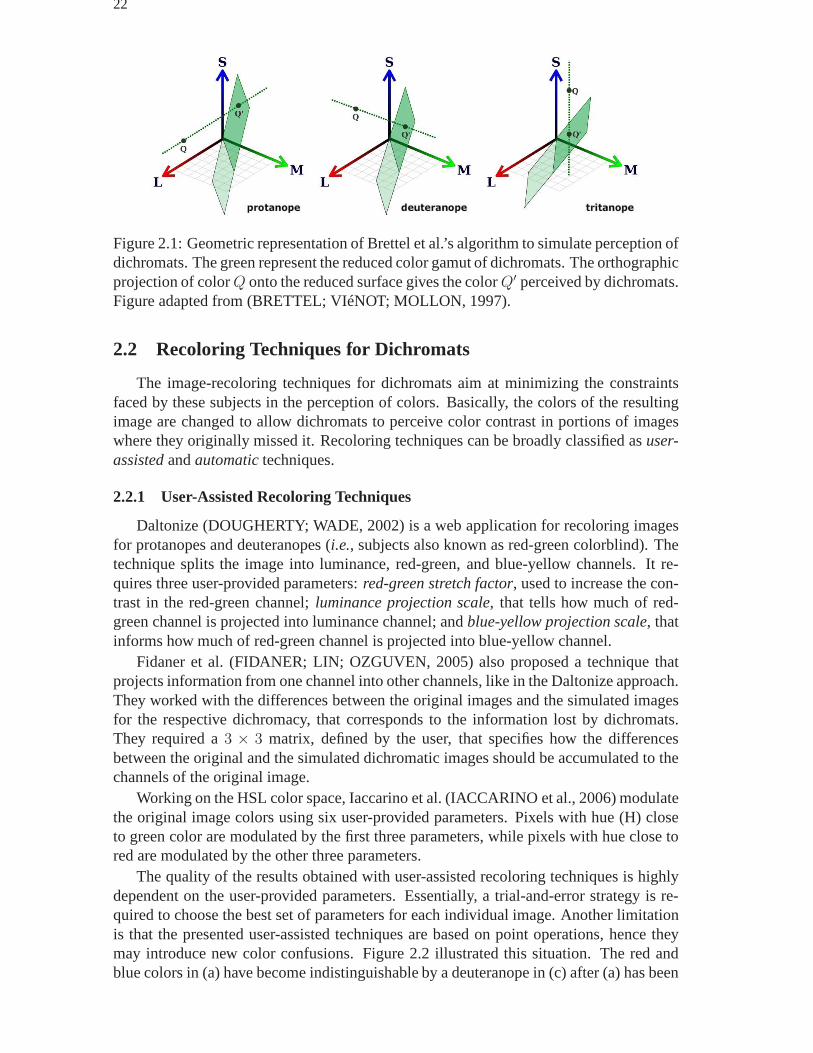
Brettel et al. use two half-planes in the LMS color space to represent the color gamutperceived by dichromats. The half-planes were based on the reports of unilateral dichro-mats in the medical literature. Each class of dichromacy hasone type of missing cone,and they confuse colors that fall along lines parallel to theaxis that represent the missingcone. Brettel et al. assumed the intersection between such lines and the half-planes asthe colors perceived by dichromats. Figure 2.1 illustratesa geometric representation ofBrettel et al.’s algorithm to simulate the perception of each class of dichromacy.

Although these simulation techniques allow individuals with normal color vision toappreciate the perception of dichromats, as we noted in the examples of Figures 1.1 to 1.3,they do not help to minimize the limitation of these individuals to perceive the contrastbetween the colors.

22

Figure 2.1: Geometric representation of Brettel et al.’s algorithm to simulate perception ofdichromats. The green represent the reduced color gamut of dichromats. The orthographicprojection of colorQ onto the reduced surface gives the colorQ′ perceived by dichromats.Figure adapted from (BRETTEL; VIéNOT; MOLLON, 1997).

2.2 Recoloring Techniques for Dichromats

The image-recoloring techniques for dichromats aim at minimizing the constraintsfaced by these subjects in the perception of colors. Basically, the colors of the resultingimage are changed to allow dichromats to perceive color contrast in portions of imageswhere they originally missed it. Recoloring techniques canbe broadly classified asuser-assisted andautomatic techniques.

2.2.1 User-Assisted Recoloring Techniques

Daltonize (DOUGHERTY; WADE, 2002) is a web application for recoloring imagesfor protanopes and deuteranopes (i.e., subjects also known as red-green colorblind). Thetechnique splits the image into luminance, red-green, and blue-yellow channels. It re-quires three user-provided parameters:red-green stretch factor, used to increase the con-trast in the red-green channel;luminance projection scale, that tells how much of red-green channel is projected into luminance channel; andblue-yellow projection scale, thatinforms how much of red-green channel is projected into blue-yellow channel.

Fidaner et al. (FIDANER; LIN; OZGUVEN, 2005) also proposed atechnique thatprojects information from one channel into other channels,like in the Daltonize approach.They worked with the differences between the original images and the simulated imagesfor the respective dichromacy, that corresponds to the information lost by dichromats.They required a3 × 3 matrix, defined by the user, that specifies how the differencesbetween the original and the simulated dichromatic images should be accumulated to thechannels of the original image.

Working on the HSL color space, Iaccarino et al. (IACCARINO et al., 2006) modulatethe original image colors using six user-provided parameters. Pixels with hue (H) closeto green color are modulated by the first three parameters, while pixels with hue close tored are modulated by the other three parameters.

The quality of the results obtained with user-assisted recoloring techniques is highlydependent on the user-provided parameters. Essentially, atrial-and-error strategy is re-quired to choose the best set of parameters for each individual image. Another limitationis that the presented user-assisted techniques are based onpoint operations, hence theymay introduce new color confusions. Figure 2.2 illustratedthis situation. The red andblue colors in (a) have become indistinguishable by a deuteranope in (c) after (a) has been

23

recolored using Fidaner et al.’s technique.

(a) (b) (c)

Figure 2.2: Example showing a limitation of user-assisted techniques based on point op-erations. (a) Color image as perceived by a subject with normal color vision. (b) Sameimage as perceived by a subject lacking green-cones (deuteranope). (c) Simulation ofdeuteranope’s perception after recoloring the image (a) using Fidaner et al.’s technique.Note that red and blue colors in (a) have become indistinguishable in (c).

2.2.2 Automatic Recoloring Techniques

Ichikawa et al. (ICHIKAWA et al., 2003) used an objective function to recolor webpages for anomalous trichromats. The objective function tries to preserve the color dif-ferences between all pairs of colors as perceived by trichromats in the reduced anomaloustrichromats’ gamut. A genetic algorithm was used to minimize the objective function.Note, however, that this problem is relatively simpler, as both groups are trichromats andno reduction in color space dimension is required. Ichikawaet al. (ICHIKAWA et al.,2004) extended their previous technique for use on color images, but they did not con-sider the preservation of color naturalness (i.e., preservation of colors that are perceivedas similar by both trichromats and anomalous trichromats).

Wakita and Shimamura (WAKITA; SHIMAMURA, 2005) proposed a technique torecolor documents (e.g., web pages, charts, maps) for dichromats using three objectivefunctions aiming, respectively, at: (i) color contrast preservation, (ii) maximum colorcontrast enforcing, and (iii) color naturalness preservation. However, in their technique,the colors for which naturalness should be preserved must bespecified by the user. Thethree objective functions are then combined by weighting user-specified parameters andoptimized using simulated annealing. They report that documents with more than 10colors could take several seconds to be optimized (no information about the specs of thehardware used to perform this time estimate were provided).

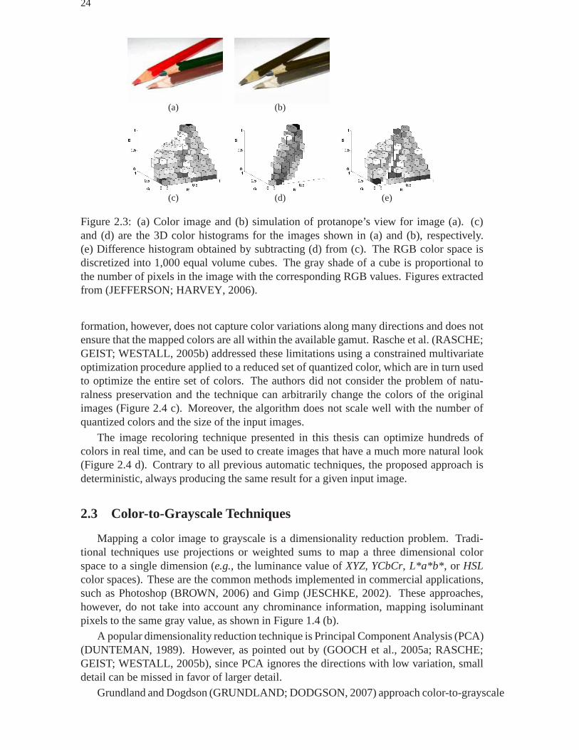
Jefferson and Harvey (JEFFERSON; HARVEY, 2006) select a setof key colors bysampling the difference histogram (Figure 2.3 e) between the trichromat’s color histogram(Figure 2.3 c) and dichromat’s color histogram (Figure 2.3 d). They use four objectivefunctions to preserve brightness, color contrast, colors in the available gamut, and colornaturalness of the selected key colors. Again, the user mustspecify the set of colors whosenaturalness should be preserved. They optimize the combined objective functions usinga method of preconditioned conjugate gradients. They report times of several minutes tooptimize a set of 25 key colors on a P4 2.0 GHz using a Matlab implementation.

Rasche et al. (RASCHE; GEIST; WESTALL, 2005a) proposed an automatic recol-oring technique for dichromats as an optimization that tries to preserve the perceptualcolor differences between all pairs of colors using an affinetransformation. Such trans-

24

(a) (b)

(c) (d) (e)

Figure 2.3: (a) Color image and (b) simulation of protanope’s view for image (a). (c)and (d) are the 3D color histograms for the images shown in (a)and (b), respectively.(e) Difference histogram obtained by subtracting (d) from (c). The RGB color space isdiscretized into 1,000 equal volume cubes. The gray shade ofa cube is proportional tothe number of pixels in the image with the corresponding RGB values. Figures extractedfrom (JEFFERSON; HARVEY, 2006).

formation, however, does not capture color variations along many directions and does notensure that the mapped colors are all within the available gamut. Rasche et al. (RASCHE;GEIST; WESTALL, 2005b) addressed these limitations using aconstrained multivariateoptimization procedure applied to a reduced set of quantized color, which are in turn usedto optimize the entire set of colors. The authors did not consider the problem of natu-ralness preservation and the technique can arbitrarily change the colors of the originalimages (Figure 2.4 c). Moreover, the algorithm does not scale well with the number ofquantized colors and the size of the input images.

The image recoloring technique presented in this thesis canoptimize hundreds ofcolors in real time, and can be used to create images that havea much more natural look(Figure 2.4 d). Contrary to all previous automatic techniques, the proposed approach isdeterministic, always producing the same result for a giveninput image.

2.3 Color-to-Grayscale Techniques

Mapping a color image to grayscale is a dimensionality reduction problem. Tradi-tional techniques use projections or weighted sums to map a three dimensional colorspace to a single dimension (e.g., the luminance value ofXYZ, YCbCr, L*a*b*, or HSLcolor spaces). These are the common methods implemented in commercial applications,such as Photoshop (BROWN, 2006) and Gimp (JESCHKE, 2002). These approaches,however, do not take into account any chrominance information, mapping isoluminantpixels to the same gray value, as shown in Figure 1.4 (b).

A popular dimensionality reduction technique is PrincipalComponent Analysis (PCA)(DUNTEMAN, 1989). However, as pointed out by (GOOCH et al., 2005a; RASCHE;GEIST; WESTALL, 2005b), since PCA ignores the directions with low variation, smalldetail can be missed in favor of larger detail.

Grundland and Dogdson (GRUNDLAND; DODGSON, 2007) approachcolor-to-grayscale

25

(a) (b) (c) (d)

Figure 2.4: Blue sky and building: (a) Color image. (b) Simulation of deuteranope’s viewfor image (a). (c) and (d) are the results produced by Rasche et al.’s and the proposedtechniques, respectively, as seen by deuteranopes. Note that colors of the sky and yellowfoliages in (a) were unnecessary changed by Rasche et al.’s approach (c), not preservingthe naturalness of such colors. Compare such a result with the one obtained with theproposed technique (d).

problem by first converting the originalRGB colors to theirY PQ color space, followedby a dimensionality reduction using a technique they calledpredominant component anal-ysis, which is similar to PCA. In order to decrease the computational cost of this analy-sis, they use a local sampling by a Gaussian pairing of pixelsthat limits the amountof color differences processed and brings the total cost to convert anN × N image toO(N2 log(N2)). This technique is very fast, but its local analysis may not capture thedifferences between spatially distant colors and, as a result, it may map clearly distinctcolors to the same shade of gray. Figure 2.5 (a) illustrates the USA time zones map us-ing distinct isoluminant colors for each time zone. Note that in the result produced byGrundland and Dogdson’s approach, shown in (c), the color contrast between some timezones (e.g., HST and AKST time zones, CST and EST time zones) were not preserved,illustrating the limitation previously described. The grayscale image (d), obtained usingour color-to-grayscale approach, successfully mapped thevarious time zones to distinctshades of gray.

Neumann et al. (NEUMANN; CADIK; NEMCSICS, 2007) presented an empiricalcolor-to-grayscale transformation algorithm based on theColoroid system (NEMCSICS,1980). Based on an user-study, they sorted the relative luminance differences betweenpairs of seven hues, and interpolated between them to obtainthe relative luminance dif-ferences among all colors. Their algorithm requires the specification of two parameters,and the reported running times are of the order of five to ten seconds per megapixel (hard-ware specs not informed).

Gooch et al. (GOOCH et al., 2005a) find gray levels that best represent the colordifference between all pair of colors by optimizing an objective function. The orderingof the gray levels arising from the original colors with different hues is resolved with auser-provided parameter. The cost to optimize anN × N image isO(N4), causing thealgorithm to scale poorly with image resolution.

Rasche et al. (RASCHE; GEIST; WESTALL, 2005b) formulated the color-to-grayscaletransformation as an optimization problem in which the perceptual color difference be-

26

(a) (b)

(c) (d)

Figure 2.5: USA time zone map: (a) Color image. (b) Luminanceimage. (c) Grayscaleimage produced by Grundland and Dogdson’s (GRUNDLAND; DODGSON, 2007)method. (d) Grayscale image obtained using the color-to-grayscale approach presented inthis thesis. Note in (c) how the color contrast between some spatially distant regions werenot preserved by Grundland and Dogdson’s approach (e.g., HST and AKST time zones,CST and EST time zones). The grayscale image shown in (d) successfully mapped thevarious time zones to different gray values.

tween any pair of colors should be proportional to the perceived difference in their corre-sponding shades of gray. In order to reduce its computation cost, the authors perform theoptimization on a reduced setQ of quantized colors, and this result is then used to opti-mize the gray levels of all pixels in the resulting image. Thetotal cost of the algorithmis O(‖Q‖2 + ‖Q‖N2). A noticeable feature of their algorithm is that in order to try tohelp the algorithm to scape local minima, the minimization procedure is initialized usinga vector of random values, which causes the algorithm to produce non-deterministic re-sults. This is illustrated in Figure 2.6, which shows the grayscale images produced in threeexecutions of their algorithm. Note that in the result shownin Figure 2.6 (b) the islandis barely visible, illustrating a situation in which the optimization got trapped in a localminima. Figure 2.6 (e) shows the result produced by the color-to-grayscale algorithmpresented in this thesis.

2.4 Summary

This chapter discussed the most relevant techniques to simulate color perception bydichromats. Although these techniques do not minimize the limitation of these individ-uals to perceive color differences, they are important because they eliminate the needfor the presence of dichromats along the development and tests of the image-recoloringalgorithms.

The chapter also presented the state-of-the-art on image-recoloring techniques for

27

(a) (b) (c) (d) (e)

Figure 2.6: Effect of the use of random numbers to initializethe algorithm by Rasche etal. (RASCHE; GEIST; WESTALL, 2005b) on the generated grayscale images. (a) Imagecontaining isoluminant colors. (b) to (d) Grayscale imagesgenerated by three executionsof the Rasche et al.’s algorithm. (e) Grayscale image produced by the color-to-grayscalealgorithm presented in this thesis. Note that in (b) the island Isle Royale National Park isbarely visible, while our color-to-grayscale technique preserved the contrast in (e).

dichromats. Basically, these techniques aim to minimize the limitations faced by thesesubjects in the perception of color contrasts. It was discussed two kind of approaches forimage recoloring: user-assisted and automatic techniques. The user-assisted recoloringtechniques, despite the low computation cost, do not take into account any analysis onthe image to choose optimal parameter settings, hence they may introduce new color con-fusions. On the other hand, automatic recoloring techniques use optimization methodsto choose the best set of colors in the dichromatic image, which tends to generate betterresults than user-assisted techniques. However, the current automatic methods are com-putationally expensive and not suitable for real-time applications. Contrary to all currentautomatic methods, the proposed image-recoloring algorithm can optimize hundreds ofcolors in real time and can produce images with more natural look.

Furthermore, this chapter presented several approaches for color-to-grayscale conver-sion. These techniques convert color images into grayscaleones with enhanced contrastby taking both luminance and chrominance into account. Unlike current optimizationmethods, the proposed color-to-grayscale technique is deterministic, can optimize hun-dreds of colors in real time, and scales well with the size of the input image.

28

29

3 MASS-SPRING SYSTEMS

This chapter reviews the basic concepts of mass-spring systems and provides the back-ground for understanding both the image-recoloring and thecolor-to-grayscale techniquesproposed in this thesis, which are cast as optimization problems.

3.1 Definition of Mass-Spring Systems

A mass-spring system consists of a set of particles (nodes) connected by springs thatdeform in the presence of some external forces, as illustrated in Figure 3.1. When com-pressed or stretched, the springs apply internal reaction forces in order to maintain theirrest length (GEORGII; WESTERMANN, 2005). The system tends to stabilize whenthe external forces are compensated by opposing internal forces. These features make amass-spring system a flexible optimization technique that optimizes a set of parameters(e.g., the positions of the particles) that best satisfy some constraints (e.g., the sum ofinternal and external forces is zero). Modeling a problem asa mass-spring system ba-sically consists of mapping some properties of the problem in hand to the variables ofthe mass-spring system: (i) particles’ positions, (ii) particles’ masses, (iii) springs’ restlengths, and (iv) springs’ current lengths. For example, anapplication could map a givenproperty of the problem as the mass of particles in the system. In this case, particles withbigger masses tend to move less. Alternatively (or in addition to this first mapping), theapplication could restrict the particles to only move alonga given axis.

Figure 3.1: Simple mass-spring system with three particles(A, B, andC), and two springs(S1 andS2). Figure extracted from (DIETRICH; COMBA; NEDEL, 2006).

Due to its properties, simplicity and low computational complexity, mass-spring sys-tems are used as an optimization tool in many areas, including body deformation andfracture, cloth and hair animation, virtual surgery simulation, interactive entertainment,and fluid animation.

30

3.2 Dynamic of Mass-Spring Systems

Considering a set of particles connected by springs, mass-spring systems are simulatedby assigning some mass to each particle and some rest length to each spring. The entiresystem must obey Newton’s second law:

Fi = miai (3.1)

wheremi is the mass of nodePi, ai is the acceleration caused by forceFi, which is thecomposition of internal and external forces. Therefore, the force applied to nodePi canbe obtained from Hooke’s law by summing the tensions of all the springs that connectPi

to its neighborsPj:

Fi =∑

j∈N

kij(1 −lijl′ij

)(pj − pi) (3.2)

whereN is the set of neighbors linked toPi, lij andl′ij are, respectively, the rest lengthand current length of the spring betweenPi andPj , kij is the stiffness of the spring, andpi andpj are the current positions ofPi andPj , respectively.

Verlet integration (VERLET, 1967) is often used to express the dynamics of eachnode. This type of integration is frequently used in simulations of small unoriented mass-points, being especially interesting when it is necessary to place constraints on the dis-tances between the points (VERTH; BISHOP, 2004). With a timestep∆t, the new posi-tion of a nodePi at timet + ∆t can be computed as:

pi(t + ∆t) =Fi(t)

mi

+ 2pi(t) − pi(t − ∆t) (3.3)

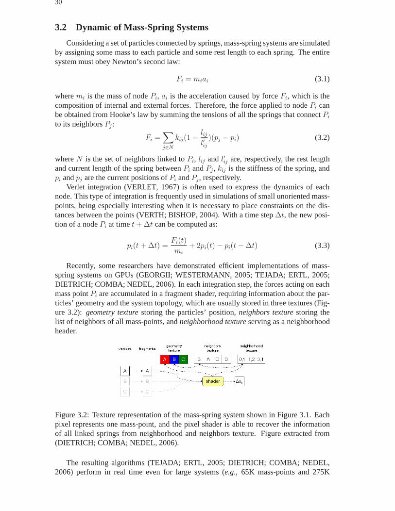
Recently, some researchers have demonstrated efficient implementations of mass-spring systems on GPUs (GEORGII; WESTERMANN, 2005; TEJADA;ERTL, 2005;DIETRICH; COMBA; NEDEL, 2006). In each integration step, the forces acting on eachmass pointPi are accumulated in a fragment shader, requiring information about the par-ticles’ geometry and the system topology, which are usuallystored in three textures (Fig-ure 3.2): geometry texture storing the particles’ position,neighbors texture storing thelist of neighbors of all mass-points, andneighborhood texture serving as a neighborhoodheader.

Figure 3.2: Texture representation of the mass-spring system shown in Figure 3.1. Eachpixel represents one mass-point, and the pixel shader is able to recover the informationof all linked springs from neighborhood and neighbors texture. Figure extracted from(DIETRICH; COMBA; NEDEL, 2006).

The resulting algorithms (TEJADA; ERTL, 2005; DIETRICH; COMBA; NEDEL,2006) perform in real time even for large systems (e.g., 65K mass-points and 275K

31

springs). The solutions proposed in this thesis for both image recoloring and color-to-grayscale transformations are cast as optimization problems and modeled as mass-springsystems with every mass pointPi connected to every other mass pointPj by a springSij.This fixed and implicitly defined topology lends itself to an efficient GPU implementation,since no topology setup is needed.

3.3 Summary

This chapter detailed the key aspects of mass-spring systems, an optimization toolwith low computational cost that can be efficient implemented both on CPU and on GPU.The understanding of the mass-spring’s dynamic is fundamental to the comprehension ofboth the image-recoloring and the color-to-grayscale techniques proposed in this thesis,as they are approached as optimization problems and modeledas mass-spring systems.

32

33

4 THE RECOLORING ALGORITHM FOR DICHROMATS

This chapter presents our image-recoloring technique for dichromats. It also analyzessome fundamental properties and guarantees of the algorithm, and introduces an extensionto the proposed method that exaggerates the color contrast in the result image. Alongthe chapter, several examples are used to illustrate the results produced by the proposedtechnique.

4.1 The Algorithm

Our image-recoloring technique for dichromats was designed to achieve the followinggoals:

• Real-time performance;

• Color naturalness preservation - It guarantees that colors of the original imageswill be preserved, as much as possible, in the resulting images;

• Global color consistency - It ensures that all pixels with the same color in the orig-inal image will be mapped to the same color in the recolored image;

• Luminance constancy - It ensures that the original luminance information of eachinput pixel will be preserved in the output one;

• Local chrominance consistency - It guarantees that chrominance order of colorsinside the same cluster will have preserved in the recoloredimage;

• Color contrast preservation - It tries to preserve the color difference between pairsof colors from the original image in the recolored one.

The proposed algorithm uses a mass-spring system to optimize the colors in the inputimage to enhance color contrast for dichromats. As presented in Section 2.1, the colorgamut of each class of dichromacy can be represented by two half-planes in the LMScolor space (BRETTEL; VIéNOT; MOLLON, 1997), which can be satisfactorily approx-imated by a single plane passing through the luminance axis (VIéNOT; BRETTEL; MOL-LON, 1999). For each class of dichromacy, we map its color gamut to the approximatelyperceptually-uniform CIE L*a*b* color space and use least-squares to obtain a planethat contains the luminance axis (i.e., L*) and best represents the corresponding gamut(Figure 4.1). This is similar to what has been described by Rasche et al. (RASCHE;GEIST; WESTALL, 2005b), who suggested the use a single planefor both protanopes

34

Figure 4.1: Approximating each dichromatic color gamut by aplane in the CIE L*a*b*color space.Θp = −11.48◦, Θd = −8.11◦, andΘt = 46.37◦.

and deuteranopes as a further simplification. Based on our least-squares fitting, the an-gles between the recovered planes and the L*b* plane areΘp = −11.48◦, Θd = −8.11◦,andΘt = 46.37◦, for protanopes, deuteranopes, and tritanopes, respectively (Figure 4.1).These angles are used to align their corresponding planes tothe L*b* plane, reducing theoptimization to 1D along the b* axis (the luminance values are kept unchanged). Afterthe optimization, the new colors are obtained by rotating the plane back.

Our algorithm has three main steps: (i)image quantization, (ii) mass-spring optimiza-tion of the quantized colors, and (iii)reconstruction of the final colors from the optimizedones. The first step consists in obtaining a setQ of quantized colors from the set of allcolorsC in the input imageI. This can be performed using any color quantization tech-nique (GONZALEZ; WOODS, 2007), such as uniform quantization, k-means, minimumvariance, median cut or color palettes.

4.1.1 Modeling the Problem as a Mass-Spring System

Working in the CIE L*a*b* color space, each quantized color~qi ∈ Q is associatedto a particlePi with massmi. The position~pi of the particlePi is initialized with thecoordinates of the perceived color by the dichromat after the gamut plane rotation:

~pi = MΘ D(~qi) (4.1)

whereD is the function that simulates the dichromat view (BRETTEL;VIéNOT; MOL-LON, 1997), andMΘ is a rotation matrix that aligns the gamut plane of the dichromatwith the L*b* plane. We connect each pair of particlesPi andPj with a springSij withelasticity coefficientkij = 1 (Equation 3.2), and rest lengthlij = ‖~qi − ~qj‖, the (Eu-clidean) distance between colors~qi and~qj in the L*a*b* space. Note that~qi and~qj are thequantized colors as perceived by a trichromat.

At each optimization step, we update the positions~pi and~pj of particlesPi andPj andcomputeSij ’s current length asl′ij = ‖~pi − ~pj‖. Given the restoring forces of the springs,the system will try to converge to a configuration for whichl′ij = lij for all Sij. Thus,after stabilization or a maximum number of iterations has been reached, the perceptualdistances between all pairs of new colors/positions(~pi, ~pj) will have approximately thesame perceptual distances as their corresponding pairs of quantized colors(~qi, ~qj) fromQ. The final setT of optimized colors~ti is obtained by applying, to each resulting color~pi, the inverse rotation used in Equation 4.1:

~ti = M−1

Θ~pi (4.2)

35

In order to enforce color naturalness preservation, we define the massmi of eachparticlePi as the reciprocal of the perceptual distance (in the L*a*b* space), between~qi

andD(~qi):

mi =1

‖~qi − D(~qi)‖(4.3)

Equation 4.3 guarantees thatany color perceived similarly by both trichromats and dichro-mats will have larges masses, causing their corresponding particles to move less. Iftrichromats and dichromats perceive~qi exactly the same way (e.g., achromatic colors),the particle would have infinite mass. In this case, we simplyset the forces acting on theparticle to zero (i.e., Fi = 0 in Equation 3.1).

4.1.2 Dealing with Local Minima

Like other optimization techniques, mass-spring systems are prone to local minima.Figure 4.2 (b) depicts the problem with a configuration obtained right after the quantizedcolors ~qi have been rotated:~qri = MΘ ~qi. In this example, particlesP1 andP2 havelarge masses (m1 is infinite) since they are perceived as having, respectively, the sameand very similar colors by trichromats and dichromats. The springs(S13, S14, S23, S24)connectingP1 andP2 to P3 andP4 apply forces that constrainP3 andP4 from movingto the other half of the b* axis (Figure 4.2 b). Figure 4.3 illustrates this situation, wherethe resulting optimized image (c) does not represent any significant improvement over theoriginal image perceived by the dichromat (b).

Once the plane that approximates the dichromat’s gamut has been aligned to the L*b*plane, pairs of ambiguous colors with considerable changesin chrominance will have theira* color coordinates with opposite signs (e.g., the red and green colors in Figure 4.2 b).We use this observation and the topology of our mass spring system to deal with localminima using the following heuristic:we switch the sign of the b* color coordinate of allrotated quantized colors whose a* coordinates are positive and whose perceptual distancebetween the color itself and how it is perceived by the class of dichromacy is bigger thansome threshold ǫ (Equation 4.4).

Although at first this heuristic might look too naive becauseone would just be replac-ing some ambiguities with another ones, it actually has somerational: (i) it avoids theambiguities among some colors found in the original image and (ii) although there is thepossibility of introducing new ambiguities, as we switch the sign of the b* coordinate forsome colors, we are also compressing and stretching their associated springs, adding tothe system a lot potential energy that will contribute to drive the solution.

Even though such a heuristic cannot guarantee that the system will never run intoa local minima, in practice, after having recolored a huge number of images, we havenot encountered yet an example in which our system was trapped by a local minimum.Figure 4.2 (c) illustrates the configuration obtained by applying the described heuristic tothe example shown in Figure 4.2 (b). Figure 4.3 (d) shows the corresponding result ofapplying this heuristic to the example shown in Figure 4.3 (a).

pb∗

i =

{

−pb∗

i if (qra∗

i > 0) and (‖~qi − D(~qi)‖ > ǫ)

pb∗

i otherwise(4.4)

In Equation 4.4,pb∗

i is the b* coordinate of color~pi andqra∗

i is the a* coordinate of therotated color~qri. The thresholdǫ enforces that colors that are perceptually similar to bothdichromats and trichromats should not have the signs of their b* coordinates switched, in

36

order to preserve the naturalness of the image. In the example illustrated by Figures 4.2and 4.3, the rotated quantized color~qr2 preserved its b* coordinate. According to ourexperience,ǫ = 15 tends to produce good results in general and was used for all imagesshown in this work.

(a) (b) (c)

Figure 4.2: Dealing with local minima. (a) A set of quantizedcolors. (b) A configuration,obtained right after plane rotation, that leads to a local minimum: sinceP1 cannot moveat all (it is an achromatic color) andP2 can only move a little bit, they will constrain theoptimization to the yellow portion of b* axis, leading the solution to a local minimum. (c)By switching the sign of the b* coordinate of~qr4, the system escapes the local minimum.

(a) (b) (c) (d)

Figure 4.3: Example of the use of a heuristic to avoid local minima: (a) Reference im-age. (b) Simulation of a deuteranope’s view of the image in (a). (c) Simulation of adeuteranope’s view after recoloring the reference image using the mass-spring optimiza-tion without the heuristic described by Equation 4.4. (d) Result produced by our techniquewith the use of Equation 4.4.

4.1.3 Computing the Final Color Values

The last step of the algorithm consists in obtaining the color values for all pixels ofthe resulting image from the set of optimized colors~tk, k ∈ {1, .., ‖T‖}, where‖T‖ isthe cardinality ofT . For this task, we have developed two distinct interpolation solutions:per-cluster interpolation andper-pixel interpolation.

37

4.1.3.1 Per-cluster interpolation

LetCk ⊂ C be a cluster formed by all colors inC that are represented by the optimizedcolor ~tk. The final value~tkm associated to the m-th color~ck

m ∈ Ck is then obtained as

~tkm = ~tk + (~d.L∗, rk~d.a∗, rk

~d.b∗) (4.5)

where~d.L∗, ~d.a∗, and~d.b∗ are respectively the L*, a*, and b* coordinates of the differencevector ~d = ( ~ck

m − ~qk). ~qk ∈ Q is the quantized color associated to the optimized color~tk. Equation 4.5 guarantees that the final color~tkm has the same luminance as~ck

m. rk is aninterpolation of ratios that indicates how close the transformed value~tk is to the optimalsolution. This interpolation is guided by Shepard’s method(SHEPARD, 1968), a standardtechnique for distance-weighted interpolation:

rk =

∑‖T‖i=1

wki‖~tk−~ti‖‖ ~qk−~qi‖

∑‖T‖i=1

wki

, for i 6= k (4.6)

wherewki = 1/‖~qk − ~qi‖2 is the distance-weighted term suggested by Shepard (SHEP-

ARD, 1968). This transformation also guarantees local chrominance consistency, as allchrominance values inside a clusterCk are computed relatively to the optimized color~tk. Equation 4.5 can be efficiently implemented both on a CPU andon a GPU. On theCPU the cost to compute all cluster ratios using Equation 4.6is O(‖Q‖2) for a setQ ofquantized colors, and the cost to interpolate each pixel using Equation 4.5 given an imagewith N × N pixels isO(N2). Thus, the total cost of computing the final image colorsfrom the setT of optimized colors isO(‖Q‖2 + N2).

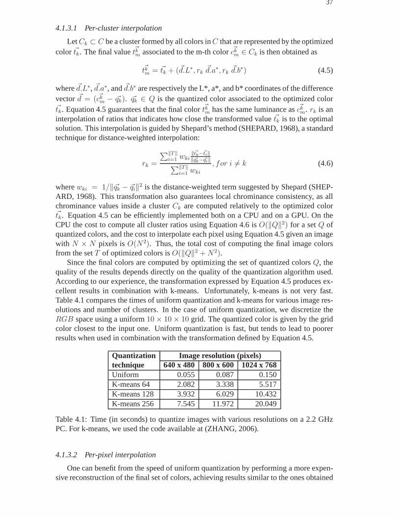
Since the final colors are computed by optimizing the set of quantized colorsQ, thequality of the results depends directly on the quality of thequantization algorithm used.According to our experience, the transformation expressedby Equation 4.5 produces ex-cellent results in combination with k-means. Unfortunately, k-means is not very fast.Table 4.1 compares the times of uniform quantization and k-means for various image res-olutions and number of clusters. In the case of uniform quantization, we discretize theRGB space using a uniform10 × 10 × 10 grid. The quantized color is given by the gridcolor closest to the input one. Uniform quantization is fast, but tends to lead to poorerresults when used in combination with the transformation defined by Equation 4.5.

Quantization Image resolution (pixels)technique 640 x 480 800 x 600 1024 x 768Uniform 0.055 0.087 0.150K-means 64 2.082 3.338 5.517K-means 128 3.932 6.029 10.432K-means 256 7.545 11.972 20.049

Table 4.1: Time (in seconds) to quantize images with variousresolutions on a 2.2 GHzPC. For k-means, we used the code available at (ZHANG, 2006).

4.1.3.2 Per-pixel interpolation

One can benefit from the speed of uniform quantization by performing a more expen-sive reconstruction of the final set of colors, achieving results similar to the ones obtained

38

when using k-means. In this case, the final shading of each pixel is obtained by opti-mizing it against the set of already optimized colorsT . This is modeled by setting up amass-spring system, and creating springs between the current pixel (treated as a particleinitialized with Equation 4.4) and all optimized colorstk, k ∈ [1, .., ‖T‖]. For this re-fining optimization stage, we force the particles associated to the shades inT to remainstationary by setting the forces acting on them to zero (Fi in Equation 3.1). For eachcolor ~cm ∈ C, we define its mass asmcm

= 1/‖ ~cm − D( ~cm)‖. This way, we allow acolor to change by an amount directly proportional to the difference of how it is perceivedby trichromats and dichromats.This mechanism guarantees the color naturalness in theresulting image.

The cost of this optimization procedure isO(‖Q‖2 + ‖Q‖N2) for anN × N image,which can be significantly higher than the mapping defined by the per-cluster interpolationtechnique (O(‖Q‖2 + N2)) for large values of‖Q‖ or N . However, since the color ofeach output pixel can be computed independently of each other, the computation canbe efficiently implemented in a fragment program. Table 4.2 compares the times forrecoloring images with various resolutions using different algorithms.MS-PC CPU andMS-PC GPU are respectively the CPU and GPU versions of our mass-springalgorithmusing per-cluster interpolation to obtain the final colors.MS-PP GPU optimizes the finalcolors using our per-pixel interpolation method as described in the previous paragraph.Table 4.2 shows that in all of its variations, our approach isa few orders of magnitudefaster than Rasche et al.’s approach. All images (and execution times) reported for thetechnique of Rasche et al. (RASCHE; GEIST; WESTALL, 2005b) were obtained usingthe software available at (RASCHE, 2005).

Recoloring Image resolution (pixels)technique 640 x 480 800 x 600 1024 x 768Rasche 225.16 349.31 580.49MS-PC CPU 0.41 0.46 0.54MS-PC GPU 0.20 0.22 0.26MS-PP GPU 0.22 0.23 0.27

Table 4.2: Performance of various algorithms on images of different resolutions. Timesmeasured in seconds on a 2.2 GHz PC with 2 GB of memory and on a GeForce 8800GTX GPU. Quantization times not included. All techniques used a set of 128 quantizedcolor. Mass-spring (MS) optimized the set of quantized colors using 500 iterations. Ourper-pixel interpolation version (MS-PP GPU) obtains the final colors using 100 iterationsfor each pixel in the image.

4.2 Exaggerated Color-Contrast

For applications involving non-natural images (e.g., scientific and information visual-ization) contrast enhancement is probably more important than preserving color natural-ness. This comes from the fact that colors used in such applications tend to be arbitrary,usually having little connection to the viewer’s previous experiences in the real world. Inscientific visualization, the details presented by the datasets are interactively explored viatransfer functions (PFISTER et al., 2001). Until now, transfer function design has largelyignored the limitations of color-vision deficients. Popular color scales usually range fromred to green, colors that are hard to be distinguished by mostdichromats.

39

By supporting real-time recoloring of transfer functions for dichromats, our approachcan assist color-vision deficient to exploit the benefits of scientific visualization. This kindof assistance can be made with the following changes in our image-recoloring algorithm:

1. Modifying the spring’s rest length to exaggerate the contrast between the colorsduring the optimization process:lij = x ‖~qi − ~qj‖, wherex is a scalar used toexaggerate the perceptual difference between any pair of color ~qi and~qj;

2. Defining the mass of particlePi as: mi = 1/‖(a∗i , b

∗i )‖, where‖(a∗

i , b∗i )‖ is the

distance from color~qi to the luminance axisL∗. Thus, less saturated colors presentbigger masses and tend to move less, as expected, this preserves the achromaticcolors;

3. Initializing the mass-spring system withǫ = 0 (Equation 4.4), since we do not needto preserve the naturalness of colors.

4.3 Results and Discussion

We have implemented the described algorithms using C++ and GLSL, and used themto recolor a large number of images. The reported times were measured using a 2.2 GHz PCwith 2 GB of memory and on a GeForce 8800 GTX with 768 MB of memory. Figures 4.4,4.5, 4.6, 4.7, and 4.8 compare the results of our technique against Rasche et al.’s approach,and Table 4.3 summarizes the performances of the algorithms. Since Rasche et al.’s tech-nique is not deterministic, for the sake of image comparison, for each example shown inthis work, we run their software five times and selected the best result. For these exper-iments, the input images were quantized using the followingalgorithms and number ofcolors: Figure 4.4 -Flowers (uniform, 227 colors), Figure 4.5 -Bell Peppers (k-means,127 colors), Figure 4.6 -Signora in Giardino (k-means, 128 colors), Figure 4.6 -Still Life(uniform, 46 colors), and Figure 4.8 -Chinese Garden (k-means, 128 colors).

Rasche et al. MS-PC CPU MS-PP GPUImage (size) Time Time TimeFlowers(839 × 602) 315.84 0.85 0.16Bell Peppers(321 × 481) 114.63 0.27 0.09Signora in Giardino(357 × 241) 60.68 0.26 0.08Still Life (209 × 333) 47.34 0.08 0.06Chinese Garden(239 × 280) 44.06 0.23 0.08

Table 4.3: Performance comparison between our technique and Rasche et al.’s for imagesof various sizes and different quantization strategies. Time measured in seconds showsthat our technique scales well with image size.

Figure 4.4,Flowers, has839× 602 pixels and our GPU implementation performed itsrecolorization in 0.158 seconds. This is2, 000× faster than Rasche et al.’s approach. OurCPU implementation was still372× faster than Rasche et al.’s for this example.

In the example shown in Figure 4.5, while Rasche et al.’s approach (c) enhanced thecontrast among the colors of the peppers, our technique alsopreserved the color natural-ness of the crates, yellow peppers, and other vegetables in the background (d).

In Figure 4.6, Monet’s paintingSignora in Giardino was recolored to enhance contrastfor protanopes. In this example, note how difficult it is for these individuals to distinguish

40

(a) (b)

(c) (d)

Figure 4.4: Images of natural flowers: (a) Photograph. (b) Same image as perceivedby protanopes (i.e., individuals without red cones). (c) Simulated view of a protanopefor a contrast-enhanced version of the photograph recolored by Rasche et al.’s approach.(d) Simulated view of a protanope for the result produced by our technique. Note how ourapproach enhanced the overall image contrast by selectively changing only the colors forwhich there is a significant perceptual difference between thrichromats and dichromats.As a result, it preserved the naturalness of the colors (fromthe perspective of the dichro-mat) of the flowers’ nuclei and of the background foliage (compare images (b) and (d)).For this 839×602-pixel image, our approach performs approximately 2,000× faster thanRasche et al.’s technique.

the red flowers from the green leaves and grass (Figure 4.6 b).Our approach clearlyimproved the perception of these flowers, while preserving the naturalness of the sky andthe other elements of the scene, as perceived by the protanope (Figure 4.6 d). Compareour results with the ones produced by Rasche et al.’s approach (c).

Figure 4.7 shows a Pablo Picasso’s painting recolored for deuteranopes. Both Rascheet al.’s result (c) and ours (d) enhanced color contrast, butonly ours preserved the natu-ralness of the yellow shades as seen by the dichromat (b).

Chinese Garden (Figure 4.8) provides an example of image recoloring for tritanopes.Note how our technique preserved the naturalness of the sky,while enhancing the contrastfor the purple flowers. Rasche et al.’s approach, on the otherhand, recolored the sky aspink and did not sufficiently enhanced the contrast of the purple flowers.

Figures 4.9 and 4.10 illustrate the use of our exaggerated color-contrast approach.Figure 4.9 shows the result of a simulated flame. Red and greencolors in (a) mean highand low temperatures, respectively. Note how difficult it isfor deuteranopes to distin-guish regions of high from regions of low temperatures in (b). Figures 4.9 (c) and (d)present the results produced by our image-recoloring and exaggerated color-contrast ap-proaches, respectively. Figure 4.10 (a) shows the visualization of carp dataset using a

41

(a) (b) (c) (d)

Figure 4.5: Color peppers: (a) Original image. (b) Simulation of a deuteranope’s viewfor image (a). (c) Simulation of a deuteranope’s view for theresults produced by Rascheet al.’s technique. (d) Simulation of a deuteranope’s view for the results produced by ourapproach, which preserved the color naturalness of the crates, the yellow peppers, andother vegetables in the background.

(a) (b)

(c) (d)

Figure 4.6: Signora in Giardino by Claude Monet, courtesy ofArtcyclopedia.com: (a)Color image. Simulated views for a protanope for: (b) the original one, (c) result producedby Rasche et al.’s approach, and (d) result produced by the proposed technique.

multi-dimensional transfer function and (b) presents thisvisualization as perceived bydeuteranopes. Note how difficult it is for deuteranopes to distinguish the colors asso-ciated to the dataset. Figures 4.10 (c) and (d) show simulated views of a deuteranopefor the results produced by our image-recoloring techniquefor dichromats and by ourexaggerated color-contrast approach, respectively.

42

(a) (b) (c) (d)

Figure 4.7: Still Life by Pablo Picasso, courtesy of Artcyclopedia.com: (a) Color image.(b) Image in (a) as perceived by subjects lacking green-cones (deuteranopes). (c) and (d)are the results of Rasche et al.’s and our techniques, respectively, as seen by deuteranopes.

(a) (b) (c) (d)

Figure 4.8: Photograph of a chinese garden: (a) Color image.Simulated views of tri-tanopes for: (b) the original image, (c) the recolored imageby Rasche et al.’s approach,and (d) the recolored image using our technique. Note the blue sky and the enhancedcontrast for the purple flowers.

43

(a) (b)

(c) (d)

Figure 4.9: Simulation of a flame: (a) Color image. Simulatedviews of deuteranopes for:(b) original image, (c) result produced by our image-recoloring technique for dichromats,and (d) result produced by our exaggerated color-contrast approach usingx = 2.

(a) (b)

(c) (d)

Figure 4.10: Visualization of a carp dataset using a multi-dimensional transfer function:(a) Color image. Simulated view of deuteranopes for: (b) original image, (c) result pro-duced by our image-recoloring technique for dichromats, and (d) result produced by ourexaggerated color-contrast approach usingx = 2.

44

4.4 Summary

This chapter presented an efficient and automatic image-recoloring algorithm for dichro-mats that, unlike the current image-recoloring methods, allows these subjects to benefitfrom contrast enhancement without having to experience toounnatural colors. The pro-posed method uses a mass-spring system to obtain the set of optimal colors in the resultingimage, and can be efficiently implemented both on CPU and on modern GPUs.

The chapter also introduced an extension to the proposed image-recoloring algorithmthat exaggerates color contrast. This kind of feature mightbe useful for applicationsdealing with non-natural images, like scientific and information visualization.

45

5 THE COLOR-TO-GRAYSCALE ALGORITHM

This chapter describes our color-to-grayscale technique that uses both luminance andchrominance information. It also introduces a new error metric for evaluating the qualityof color-to-grayscale transformations and discusses the results obtained with the proposedtechnique.

5.1 The Algorithm

Our color-to-grayscale algorithm is a specialization of the recoloring algorithm fordichromats presented in Chapter 4. In the recoloring algorithm, we searched for an opti-mal color contrast after projecting samples from a 3D color space into the 2D color gamutof a dichromat. For the color-to-grayscale problem, we search for the optimal contrastafter projecting samples of a 3D color space now into a 1D color space. For this purpose,many of the same strategies used in the previous chapter can be reused here. Not surpris-ingly, both algorithms have many things in common, including the number and order ofthe steps, and the use of a mass-spring system as the optimization tool.

Thus, like the previous proposed algorithm, this one also has three main steps. Thefirst step consists in obtaining a setQ of quantized colors from the set of all colorsC in theinput imageI, and can be performed using any color quantization technique. The secondstep performs a constrained optimization on the values of the luminance channel of thequantized colors using a mass-spring system. At this stage,the chrominance informationis taken into account in the form of constraints that specifies how much each particle canmove (Section 5.1.1). The final gray values are reconstructed from the set of gray shadesproduced by the mass-spring optimization (Section 5.1.2).This final step guarantees localluminance consistency preservation.

5.1.1 Modeling and Optimizing the Mass-Spring System

Similar to the recoloring algorithm for dichromats, the color-to-grayscale mapping ismodeled as a mass-spring system whose topology is a completegraph (i.e., each particlePi is connected to each other particlePj by a springSij with fixed stiffnesskij = 1).Each particlePi is associated to a quantized color~qi ∈ Q (represented in the almostperceptually uniform CIE L*a*b* color space) containing some massmi. Here, however,the particles are only allowed to move along the L*-axis of the color space and eachparticlePi has its positionpi (in 1D) initialized with the value of the luminance coordinateof ~qi. Between each pair of particles(Pi, Pj), we create a spring with rest length given by

lij =Grange

Qrange

‖~qi − ~qj‖ (5.1)

46

whereQrange is the maximum difference between any pair of quantized colors in Q,Grange is the maximum possible difference between any pair of luminance values, and‖~qi − ~qj‖ approximates the perceptual difference between colors~qi and ~qj . Note thatsince the luminance values are constrained to theL∗-axis,Grange = 100.

The instantaneous force applied to a particlePi is obtained by summing the tensions ofall springs connectingPi to its neighborsPj, according to Hooke’s law (Equation 3.2). Ateach step of the optimization, we updatel′ij as|L∗

i −L∗j |, and the new positionpi (actually

the gray levelL∗i ) according to Verlet’s integration (Equation 3.3). The resulting system

tends to reach an equilibrium when the perceptual differences between the optimized graylevels are proportional to the perceptual differences among the quantized colors inQ.

In order to enforce grayscale preservation, we set the massmi of particlePi as thereciprocal of the magnitude of~qi’s chrominance vector (Figure 5.1):

mi =1

‖(a∗i , b

∗i )‖

(5.2)

Note thatd = ‖(a∗i , b

∗i )‖ is the distance from color~qi to the luminance axisL∗. Thus,

less saturated colors present bigger masses and tend to moveless. For achromatic colors,whose mass should be infinity, we avoid the division by zero simply by settingFi = 0(Equation 3.2). This keeps achromatic colors stationary.

Figure 5.1: The mass of particle associated with a quantizedcolor ~qi is computed as thereciprocal of its distanced to the luminance axisL∗: mi = 1/(‖(a∗

i , b∗i )‖). This enforces

grayscale preservation, as achromatic colors will remain stationary.

5.1.2 Interpolating the Final Gray Image

The last step of the algorithm consists in obtaining the grayvalues for all pixels ofthe resulting image. For this task, we have adapted the two approaches described inSections 4.1.3.1 and 5.1.2.2:per-cluster interpolation andper-pixel interpolation. Thechoice for one interpolation method depends on the application requirements.

5.1.2.1 Per-cluster interpolation

Consider the setqk ∈ Q of quantized colors and the respective associated setgk ∈ Gof optimized gray levels. LetCk ⊂ C be a cluster composed of all colors inC that in theoptimization are represented by the quantized color~qk. The final gray level associated tothem-th color ~ck

m ∈ Ck is then obtained as

gray( ~ckm) =

{

gk + rk‖~qk − ~ckm‖ lum( ~ck

m) ≥ lum(~qk)

gk − rk‖~qk − ~ckm‖ otherwise

(5.3)

47

wherelum is the function that returns the coordinate L* of a color in the L*a*b* colorspace, andrk is Shepard’s (SHEPARD, 1968) interpolation of ratios, in this case com-puted as

rk =

∑‖Q‖i=1

wki|gk−gi|‖ ~qk−~qi‖

∑‖Q‖i=1

wki

, for i 6= k (5.4)

rk indicates how close to the optimal solution is the gray valuegk, andwki = 1/‖~qk−~qi‖2

is the distance-weighted term. For the quantized color~qk that represents the cluster, allgray values inside thek-th cluster are computed with respect to the optimized gray levelgk. Therefore, this transformation ensures local luminance consistency.

Again, given the setQ of quantized colors, the cost of computing all cluster ratiosusing Equation 5.4 on the CPU isO(‖Q‖2), while the cost of interpolating each pixel ofan image withN × N pixels isO(N2).

5.1.2.2 Per-pixel interpolation

In this approach, each pixel’s final shading is computed by optimizing it against thesetgk ∈ G of previously optimized gray levels. This is achieved by using a mass-springsystem, with springs connecting the current pixel (which istreated as a particle initializedwith the pixel´s luminance value) and all optimized gray levelsgk. In this refined opti-mization stage, the particles associated to the optimized gray levels are kept stationaryby setting the forces that act on them to zero (Fi in Equation 3.2). Equation 5.2 is thenused to obtain the mass of the pixel being optimized. In this stage, all pixels with achro-matic colors endup having infinite masses, remaining stationary. This ensures that all grayshades in the original color image will be preserved in the resulting grayscale image.

5.2 Error Metric for Color-to-Grayscale Mappings

We introduce an error metric to evaluate the quality of color-to-grayscale transforma-tions. It consists of measuring whether the difference between any pairs of colors(~ci,~cj)in the original color image have been mapped to the corresponding target difference inthe grayscale image. For this purpose, we defined an error function using root weightedmean square (RWMS):

rwms(i) =

√

1

‖K‖

∑

j∈K

1

δ2ij

(δij − |lum(~ci) − lum(~cj)|)2 (5.5)

where,rwms(i) is the error computed for theith pixel of the input color imageI, K isthe set of all pixels inI, ‖K‖ is the number of pixels inI, δij = (Grange/Crange)‖~ci -~cj‖ is the target difference in gray levels for a pair of colors~ci and ~cj, and lum is thefunction that return the component L* of a color. Since the differences are computed inthe approximate perceptually uniform L*a*b* color space,Grange = 100 andCrange isthe maximum distance between any two colors in the color image I. The weight(1/δ2

ij)is used to suppress the bias toward large values ofδij .

For anN ×N image, evaluating Equation 5.5 for every pixel ofI would takeO(N4),which becomes impractical for large values ofN . We can obtain a very good approxima-tion to this error function by restricting the computation to the setqj ∈ Q of quantized

48

colors, given by:

rwmsq(i) =

√

√

√

√

1

‖K‖

∑

j∈Q

‖Kj‖

δqij

2

(

δqij − |lum(~ci) − lum(~qj)|

)2(5.6)

In Equation 5.6,Kj ⊂ K is the cluster of pixels represented by the quantized color~qj, δq

ij = (Grange/Qrange)‖~ci − ~qj‖, ~ci is the color of thei-th pixel, andQrange isthe maximum distance between any two quantized colors inQ. We have compared theRWMS values produced by Equations 5.5 and 5.6 for a set of 50 images of natural scenes,paintings, charts, and maps. From this study, we found that the average relative differ-ence between the two results was only1.47%. Given these relatively small differencesbut its significantly smaller costO(‖Q‖N2), all contrast errors shown in this work werecomputed using the metric represented by Equation 5.6. Also, in all contrast error imagesshown in this thesis, the green shade shown at the bottom of the error color ramp indicatesrwms = 0.0, while the red shade at the top representsrwms = 1.2.

Figure 5.2 illustrates the use of our contrast error metric.Figure 5.2 (c) is the errorimage for the pair of color and grayscale images shown on Figures 5.2 (a) and (b), re-spectively, using a set of 64 quantized colors. The grayscale image was obtained as theluminance of image (a). As expected, the largest errors concentrate on the berries pixels,since these present the biggest contrast lost. Smaller errors are spread over the severalgreen shades of the leaves.

(a) (b) (c) (d)

Figure 5.2: Example of our contrast error metric. (a) Color image. (b) Luminance im-age of (a). (c) Error image computed using Equation 5.6. The largest contrast errorsconcentrate on the berry pixels.

Figure 5.3 illustrates the impact of the weighting term1/δqij

2 on the metric. Figure 5.3(b) shows a luminance image obtained from (a). The contrast error image is shown inFigure 5.3 (c) and was computed from a set of 128 quantized colors. The error imageshown in (d) was computed using the RMS error (i.e., removing the weighting term fromEquation 5.6). Note that the region around the head of the butterfly has bigger contrasterror, which has been captured by the error image in (c), while it was missed by the RMSerror image shown in (d).

5.3 Results and Discussion

The described algorithms have been implemented in C++ and GLSL, and used themdecolorize a very large number of images. The reported timeswere measured using a 2.2GHz PC with 2 GB of memory and on a GeForce 8800 GTX with 768 MB ofmemory.

49

(a) (b) (c) (d) (e)

Figure 5.3: (a) Color image, (b) the luminance version of image (a), (c) RWMS errorimage. Note the perceptual error around the head of the butterfly, and (d) RMS errorimage.

Figure 5.4 compares the times for quantization and decolorizing images with variousresolutions using different algorithms. Using the same notation introduced in the pre-vious chapter,MS-PC CPU is our mass-spring algorithm using per-cluster interpolationin combination with k-means, andMS-PP GPU is our mass-spring algorithm using per-pixel interpolation with uniform quantization. In the caseof k-means, we used a set of128 colors and the code available at (ZHANG, 2006). In the case of uniform quantiza-tion, we discretized theRGB space using an uniform10×10×10 grid. Figure 5.4 showsthat in all of its variations, our approach is a few orders of magnitude faster than bothGooch et al.’s and Rasche et al.’s approaches. All images andexecution times shown inthis work regarding the techniques of Gooch et al. (GOOCH et al., 2005a) and Rascheet al. (RASCHE; GEIST; WESTALL, 2005b) were obtained using software provided bythese authors at (GOOCH et al., 2005b) and (RASCHE, 2005), respectively.

Figure 5.5 compares the results produced by various techniques with respect to grayscalepreservation. One should note that only the luminance image(b) and the result producedby our method (f) are capable of preserving the original shades of gray. The luminanceimage, however, failed to distinguish the shades of the various isoluminant circles. Goochet al.’s (Figure 5.5 c) and Rasche et al.’s (Figures 5.5 d and e) techniques changed theoriginal gray shades in the resulting images.

Figures 5.6, 5.8, 5.9, and 5.10 compare the results, performance, and the overall con-trast errors produced by the various algorithms. Table 5.1 summarizes these data. Follow-ing the authors comments on image quality, we did not use any quantization with Goochet al.’s algorithm. For Rasche et al.’s and ours, the input images were quantized as shownon the second column of Table 5.1.

Table 5.1 also shows that our approach simultaneously presents the smallest RWMSerror and is by far faster than Gooch et al.’s and Rasche et al.’s techniques. The luminanceimage, on the other hand, presents the biggest overall contrast errors, which is somethingthat was already expected, since the color-to-luminance mapping completely ignores thechrominance information of the original image.

Figure 5.6 shows four grayscale renditions of Claude Monet’s Impressionist Sunrise(Figure 5.7), with their respective contrast error images obtained using our metric. Thisexample illustrates the robustness of our technique to handle large images. TheSunrisehas(839× 602) pixel and our GPU implementation performs the decolorization in 0.435seconds. This is751× faster than Rasche et al.’s approach and77, 910× faster than Goochet al.’s. Our CPU implementation is still247× faster than Rasche et al.’s and25, 379×

50

64

0x4

80

80

0x6

00

10

24

x7

68

64

0x4

80

80

0x6

00

10

24

x7

68

64

0x4

80

80

0x6

00

10

24

x7

68

64

0x4

80

80

0x6

00

10

24

x7

68

64

0x4

80

80

0x6

00

0

20

40

60

80

100

120

140

160

180

200

220

Tim

e (

seconds)

Quantization

Decolorization

MS-PC CPUK-Means

MS-PP GPUUniform

Rasche et al.K-Means

Rasche et al.Uniform

Gooch et al.

...

...

0

0.2

0.4

64

0x4

80

80

0x6

00

10

24

x7

68

MS-PP GPUUniform

Figure 5.4: Performance comparison of various algorithms on a 2.2 GHz PC with 2 GBof memory and on a GeForce 8800 GTX GPU using images of different resolutions.Gooch et al. performed in 12,276 and 30,372 seconds for(640 × 480) and(800 × 600)-pixel images, respectively. Except for Gooch et al., all other techniques used a set of 128quantized colors. Our mass-spring (MS) approaches optimized the set of quantized colorsusing 1,000 iterations. TheGPU version obtained the final gray levels by optimizing eachpixel with 100 iterations. Its results are detailed for better visualization. Note how theproposed approach scales well with the size of the input images.

faster than Gooch et al.’s.Picasso Lovers (Figure 5.8) provides an example for which the result produced by

Gooch et al.’s technique presents a large contrast error (Figure 5.8 h). For this same image,Rasche et al.’s approach produced a relatively small contrast error, but in the resultinggrayscale image it is hard to distinguish between the lady’syellow skirt and the man’s redclothes. For the photograph shown in Figure 5.9, the overallcontrast error produced byGooch et al.’s technique (Figure 5.9 h) is about the same as the one found in the luminanceimage (Figure 5.9 g).

Figure 5.10 illustrates the difficulty of Rasche et al.’s approach to capture some subtleshading variations among isoluminant colors. In this example, the smooth yellow halloaround the butterfly’s head has been missed, while it was captured by Gooch et al.’s andour techniques.

51

(a) (b) (c) (d) (e) (f)

Figure 5.5: Example of grayscale preservation. (a) Original color image with isoluminantcircles; (b) Luminance image obtained from (a). Note it mapsall isoluminant circle to thesame shade of gray; (c) Result produced by Gooch et al.’s technique. Note that the twoshades of green and the shade of orange turned into white in the resulting image; (d) and(e) are two results produced by Rasche et al.’s approach. (f)Grayscale image producedby our approach; Note that only the luminance image (b) and the result produced by ourapproach (f) preserved the original gray shades. The results shown in (d), (e) and (f) tooka set of seven uniformly quantized colors as input.

Label Image (size) Quant. (#colors)#1 Sunrise(839 × 602) uniform (264)#2 Lovers(301 × 407) k-means (255)#3 Boats(193 × 282) uniform (141)#4 Butterfly (128 × 164) k-means (120)

Image Lum. Gooch et al. Rasche et al. MS-PC CPU MS-PP GPULabel RWMS Time RWMS Time RWMS Time RWMS Time RWMS

#1 0.707 33,501.4 0.557 326.78 0.564 1.32 0.429 0.43 0.425#2 0.690 1,882.5 0.699 87.36 0.498 0.96 0.486 0.36 0.477#3 0.634 328.3 0.624 20.10 0.513 0.35 0.432 0.17 0.428#4 0.582 57.3 0.535 5.54 0.443 0.21 0.365 0.15 0.362

Table 5.1: Summary of the performance and overall contrast error produced by the varioustechniques when applied to the test images. Time measured inseconds. Our approachpresents the smallest RWMS error for all examples and is significantly faster than theother techniques. The speedups increase with the image sizes. For theSunrise image,with (839 × 602) pixel, our GPU implementation is751× faster than Rasche et al.’s(CPU) approach and77, 910× faster than Gooch et al.’s (CPU).

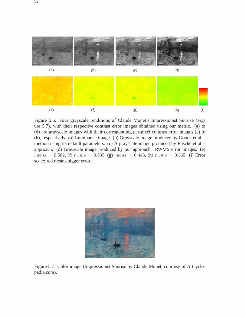
52

(a) (b) (c) (d)

(e) (f) (g) (h) (i)

Figure 5.6: Four grayscale renditions of Claude Monet’s Impressionist Sunrise (Fig-ure 5.7), with their respective contrast error images obtained using our metric. (a) to(d) are grayscale images with their corresponding per-pixel contrast error images (e) to(h), respectively. (a) Luminance image. (b) Grayscale image produced by Gooch et al.’smethod using its default parameters. (c) A grayscale image produced by Rasche et al.’sapproach. (d) Grayscale image produced by our approach. RWMS error images: (e)rwms = 0.582, (f) rwms = 0.535, (g) rwms = 0.443, (h) rwms = 0.365. (i) Errorscale: red means bigger error.

Figure 5.7: Color image (Impressionist Sunrise by Claude Monet, courtesy of Artcyclo-pedia.com).

53

(a) (b) (c) (d) (e)

(f) (g) (h) (i) (j)

Figure 5.8: Pablo Picasso’s Lovers: (a) Color image (courtesy of Artcyclopedia.com). (b)to (e) are grayscale images with their per-pixel contrast error images (g) to (j), respec-tively. (b) Luminance image. (c) Grayscale image produced by Gooch et al.’s method us-ing its default parameters. (d) A grayscale image produced Rasche et al.’s approach. Notethat it is hard to distinguish between the lady’s yellow skirt and the man’s red clothes.(e) Grayscale image produced by our approach. (f) Error scale: red means bigger error.RWMS error images: (g) to (j).

54

(a) (b) (c) (d) (e)

(f) (g) (h) (i) (j)

Figure 5.9: Photograph of a natural scene: (a) Color image. (b) to (e) are grayscale imageswith their per-pixel contrast error images (g) to (j), respectively. (b) Luminance image.(c) Grayscale image produced by Gooch et al.’s method using its default parameters. (d)A grayscale image produced Rasche et al.’s approach. (e) Grayscale image produced byour approach. (f) Error scale: red means bigger error.(g) to(j).

55

(a) (b) (c) (d) (e)

(f) (g) (h) (i) (j)

Figure 5.10: Butterfly: (a) Color image. (b) to (e) are grayscale images with their per-pixel contrast error images (g) to (j), respectively. (b) Luminance image. (c) Grayscaleimage produced by Gooch et al.’s method using its default parameters. (d) A grayscaleimage produced Rasche et al.’s approach. (e) Grayscale image produced by our approach.(f) Error scale: red means bigger error. RWMS error images: (g) to (j).

56

5.4 Summary

This chapter described a new color-to-grayscale techniquethat uses both luminanceand chrominance information to preserve the contrast, found in the input color image, inthe resulting grayscale one. The proposed method is based ona mass-spring optimizationand is almost three orders of magnitude faster than current optimization-based techniques.

This chapter also presented an error metric for evaluating the quality of color-to-grayscale transformations. It measures the error between the differences of any pairsof colors in the original image and the corresponding differences in the grayscale image.The proposed metric is based on a RWMS error.

57

6 CONCLUSIONS

This thesis presented an efficient naturalness-preservingimage-recoloring algorithmfor dichromats based on mass-spring optimization. Contrary to previous automatic tech-niques, the proposed method allows dichromats to benefit from contrast enhancementwithout having to experience unnatural colors. Besides being deterministic, our techniquehas many attractive properties: (i) it satisfies global color consistency; (ii) ensures lumi-nance constancy; (iii) maintains local chrominance consistency; and (iv) can be efficientlyimplemented on modern GPUs. Both CPU and GPU versions of the proposed algorithmare significantly faster than previous approaches (ICHIKAWA et al., 2004; WAKITA;SHIMAMURA, 2005; RASCHE; GEIST; WESTALL, 2005b; JEFFERSON; HARVEY,2006). It has also presented an extension to our image-recoloring method that exagger-ates the color contrast for dichromats in the result image. Such a feature is useful forapplications involving non-natural images (e.g., scientific and information visualization).

A second contribution of this thesis is an efficient mass-spring-based approach forcontrast enhancement during color-to-grayscale image conversion. The proposed methodis more than three orders of magnitude faster than previous optimization-based tech-niques (GOOCH et al., 2005a; RASCHE; GEIST; WESTALL, 2005b), while producingsuperior results both in terms of contrast preservation andimage guarantees. Our algo-rithm satisfies a global consistency property, preserves grayscale values present in thecolor image, maintains local luminance consistency, is completely automatic, and can beefficiently implemented on modern GPUs.

Another contribution of this thesis is an error metric for evaluating the quality ofcolor-to-grayscale transformations. The proposed metricis based on a RWMS error thatmeasures whether the difference between any pairs of colorsin the original image havebeen mapped to the corresponding target difference in the grayscale image.

The quality of the results produced by our image-recoloringand color-to-grayscaletechniques depend on the quality of quantization performedin their first stage. For low-quality images, the quantization algorithm may fail to generate a good set of quantizedcolors, causing the result images to exhibit artifacts. Although we ensure a continuousmapping among the colors/gray-shades in any given cluster,currently the algorithms donot ensure a continuous mapping among different clusters. In practice, however, after ex-tensive tests on a large number of images, we have not noticedany objectionable artifactsdue to these limitations.

This work opens up several avenues for future exploration. As the proposed ap-proaches were designed to deal with static images, we plan toexplore ways to extendour techniques to perform video sequences recolorization/decolorization. Preliminaryresults show that we can enforce temporal coherence by initializing the mass-springoptimization with particles computed for previous frames,and by keeping those parti-

58

cles stationary. Temporal coherence is not preserved by related techniques (GOOCHet al., 2005a; GRUNDLAND; DODGSON, 2007; JEFFERSON; HARVEY, 2006; NEU-MANN; CADIK; NEMCSICS, 2007; RASCHE; GEIST; WESTALL, 2005b; WAKITA;SHIMAMURA, 2005).

We believe that our image-recoloring technique can have a positive impact on the waydichromats interact with digital media, as it finally provides a practical way of disam-biguating colors without contradicting, as much as possible, their memories about howthe world looks like. We hope these results will inspire the design of new applicationsand interfaces for dichromats.

With regarding to our color-to-grayscale technique, the unique combination of high-fidelity capture of color differences, grayscale preservation, global consistency, local lu-minance consistency, and speed makes our technique a good candidate for replacing stan-dard luminance-based color-to-grayscale algorithms in printing and pattern recognitionapplications.

59

REFERENCES

ABI Research.Game Industry Revenue Expected To Double By 2011. 2006.

BRETTEL, H.; VIéNOT, F.; MOLLON, J. D. Computerized simulation of color appear-ance for dichromats.J. Opt. Soc. Am., [S.l.], v.14, n.10, p.2647–2655, 1997.

BROWN, R.Photoshop: converting color to black-and-white. 2006.

ENGEL, W. (Ed.).Storing and Accessing Topology on the GPU: a case study on mass-spring systems. [S.l.: s.n.], 2006. p.565–578.

DOUGHERTY, R.; WADE, A. Daltonize. Accessed on Oct/06,(http://www.vischeck.com/daltonize).

DUNTEMAN, G. Principal Components Analysis. [S.l.]: Sage Publications, Inc., 1989.

FIDANER, O.; LIN, P.; OZGUVEN, N.Analysis of Color Blindness - Project Writeup.2005.

GEORGII, J.; WESTERMANN, R. Mass-Spring Systems on the GPU.Simul. ModellingPractice and Theory, [S.l.], v.13, p.693–702, 2005.

GONZALEZ, R. C.; WOODS, R. E.Digital Image Processing. 3ed. ed. [S.l.]: PrenticeHall, 2007.

GOOCH, A. A.; OLSEN, S. C.; TUMBLIN, J.; GOOCH, B. Color2Gray: salience-preserving color removal.ACM Trans. Graph. , New York, NY, USA, v.24, n.3, p.634–639, 2005.

GOOCH, A. A.; OLSEN, S. C.; TUMBLIN, J.; GOOCH, B.Color2Gray: salience-preserving color removal. 2005.

GRUNDLAND, M.; DODGSON, N. A. Decolorize: fast, contrast enhancing, color tograyscale conversion.Pattern Recogn., New York, NY, USA, v.40, n.11, p.2891–2896,2007.

HEATH, G. The Handicap of Color Blindness.Journal of the American OptometricAssociation, [S.l.], v.45, n.1, p.62–69, 1974.

IACCARINO, G.; MALANDRINO, D.; PERCIO, M. D.; SCARANO, V. Efficient edge-services for colorblind users. In: WWW ’06, 2006.Proceedings. . .[S.l.: s.n.], 2006.p.919–920.

60

ICHIKAWA, M.; TANAKA, K.; KONDO, S.; HIROSHIMA, K.; ICHIKAW A, K.; TAN-ABE, S.; FUKAMI, K. Web-Page Color Modification for Barrier-Free Color Vision withGenetic Algorithm.Lecture Notes in Computer Science, [S.l.], v.2724, p.2134–2146,2003.

ICHIKAWA, M.; TANAKA, K.; KONDO, S.; HIROSHIMA, K.; ICHIKAW A, K.; TAN-ABE, S.; FUKAMI, K. Preliminary study on color modification for still images to realizebarrier-free color vision. In: IEEE SMC ’06, 2004.Anais. . . [S.l.: s.n.], 2004. v.1, p.36–41.

Id Software, Inc.(http ://www.idsoftware.com/). Accessed on May/06.

JEFFERSON, L.; HARVEY, R. Accommodating color blind computer users. In: ASSETS’06, 2006.Proceedings. . .[S.l.: s.n.], 2006. p.40–47.

JESCHKE, E. R.GIMP : converting color images to b&w. Accessed in Aug/07,(http://www.gimp.org/tutorials/Color2BW/).

JUDD, D. B. Color perceptions of deuteranopic and protanopic observers.J. Res. Natl.Bur. Std., [S.l.], v.41, p.247–271, 1948.

MEYER, G. W.; GREENBERG, D. P. Color-defective vision and computer graphics dis-plays.IEEE Comput. Graph. Appl. , [S.l.], v.8, n.5, p.28–40, 1988.

NEMCSICS, A. Coloroid Color System.Color Research and Application, [S.l.], v.5,p.113–120, 1980.

NEUMANN, L.; CADIK, M.; NEMCSICS, A. An Efficient Perception-Based Adap-tive Color to Gray Transformation. In: COMPUT. AESTHETICS,2007.Proceedings. . .[S.l.: s.n.], 2007. p.73– 80.

PFISTER, H.; LORENSEN, B.; BAJAJ, C.; KINDLMANN, G.; SCHROEDER, W.;AVILA, L. S.; MARTIN, K.; MACHIRAJU, R.; LEE, J. The TransferFunction Bake-Off. IEEE Comput. Graph. Appl. , Los Alamitos, CA, USA, v.21, n.3, p.16–22, 2001.

RASCHE, K.Detail Preserving Color Transformation. 2005.

RASCHE, K.; GEIST, R.; WESTALL, J. Detail Preserving Reproduction of Color Imagesfor Monochromats and Dichromats.IEEE Comput. Graph. Appl. , Los Alamitos, CA,USA, v.25, n.3, p.22–30, 2005.

RASCHE, K.; GEIST, R.; WESTALL, J. Re-coloring Images for Gamuts of Lower Di-mension.Comput. Graph. Forum, [S.l.], v.24, n.3, p.423–432, 2005.

RIGDEN, C. The Eye of the Beholder - Designing for Colour-Blind Users.BritishTelecommunications Engineering, [S.l.], v.17, 1999.

GEGENFURTNER, K. R.; SHARPE, L. T. (Ed.).Color Vision: from genes to percep-tion. [S.l.]: Cambridge University Press, 1999. p.3–51.

SHEPARD, D. A two-dimensional interpolation function for irregularly-spaced data.In: ACM NATIONAL CONFERENCE, 1968., 1968.Proceedings. . .[S.l.: s.n.], 1968.p.517–524.

61

SLOAN, L. L.; WOLLACH, L. Case of unilateral deuteranopia.J. Opt. Soc. Am., [S.l.],v.38, n.6, p.502, 1948.

TEJADA, E.; ERTL, T. Large Steps in GPU-based Deformable Bodies Simulation.Simu-lation Practice and Theory, [S.l.], v.Special Issue on Programmable Graphics Hardware,p.703–715, 2005.

VERLET, L. Computer "Experiments" on Classical Fluids. I. Thermodynamical Proper-ties of Lennard-Jones Molecules.Phys. Rev., [S.l.], v.159, n.1, p.98, Jul 1967.

VERTH, J. M. V.; BISHOP, L. M.Essential Mathematics for Games and InteractiveApplications. [S.l.]: Morgan Kaufmann, 2004.

VIéNOT, F.; BRETTEL, H. Color display for dichromats. In: SPIE, 2000.Proceedings. . .[S.l.: s.n.], 2000. v.4300, p.199–207.

VIéNOT, F.; BRETTEL, H.; MOLLON, J. D. Digital Video Colourmaps for Checkingthe Legibility of Displays by Dichromats.Color Research and Application, [S.l.], v.24,p.243–252, 1999.

WAKITA, K.; SHIMAMURA, K. SmartColor: disambiguation framework for the color-blind. In: ASSETS ’05, 2005.Proceedings. . .[S.l.: s.n.], 2005. p.158–165.

WALRAVEN, J.; ALFERDINCK, J. W. Color displays for the colorblind. In: IS&TAND SID 5TH COLOR IMAGING CONFERENCE, 1997.Anais. . . [S.l.: s.n.], 1997.p.17–22.

WANDELL, B. A. Foundations of Vision. [S.l.]: Sinauer Association, 1995.

ZHANG, R. K-means clustering. 2006.