Image Formation
112
1 Digital Image Processing Image Formation Dr. Muhammad Jehanzeb Department of CS Fatima Jinnah Women University Rawalpindi
-
Upload
findingnemo4 -
Category
Documents
-
view
229 -
download
1
description
Digital Image Process Slides, Godzilla
Transcript of Image Formation

1
Digital Image Processing
Image Formation
Dr. Muhammad Jehanzeb
Department of CSFatima Jinnah Women University
Rawalpindi

2
Image Formationob
ject
image planelens

3
Image Formation
light
sour
ce

4
Image Formation
projection through lens
projection through lens
image of objectimage of object

5
Image Formation
projection onto discrete sensor array
projection onto discrete sensor array digital cameradigital camera

6
Image Formation
Digital Image is an approximation of a real world scene
Sam
plin
gS
ampl
ing

7
Image Formation
sensors register average color
sensors register average color
sampled imagesampled image

8
Image Formation
Digital Image is an approximation of a real world scene
Qua
ntiz
atio
nQ
uant
izat
ion

9
Image Formation

10
Sampling and Quantization
pixel grid
sampledreal image quantized sampled & quantized

Quantization: Example
0
5
10
15
20
25
30
35
40
45
50
0 5 10 15 20 25 30 35 40 45 50
Actual change
Cha
nge
you
retu
rn
For Rs. 2 Return 5
For Rs. 7 Return 5
For Rs. 9 Return 10
For Rs. 12 Return 10
For Rs. 23 Return 25
…. ….

12
Image Formation - Quantization
continuous color input
disc
rete
col
or o
utpu
t
continuous colors mapped to a finite,
discrete set of colors.
continuous colors mapped to a finite,
discrete set of colors.

13
Sampling and Quantization
Sampling: Digitization of the spatial coordinates (x,y)
Quantization: Digitization in amplitude (also known as gray level
quantization)

14
Sampling and Quantization
Quantization 8 bit quantization: 28 =256 gray levels (0: black, 255: white) 1 bit quantization: 2 gray levels (0: black, 1: white) – binary
Sampling Commonly used number of samples (resolution)
Digital still cameras: 640x480, 1024x1024, up to 4064 x 2704 Digital video cameras: 640x480 at 30 frames/second (fps)

15
Digital Image Representation

16
Digital Image Representation
11 1
1
An
m mn
a a
a a
Divided into 8x8 blocks

17
Digital Image Representation
Number of intensity levels – An integer power of 2
Intensity levels
Dynamic range – Range of values spanned by the gray
scale
2kL
0, 1L

18
Digital Image Representation
Image Size Number of bits required to store an image
Image having 2k intensity levels k – bit image
256 intensity levels – 8 bit image
b M N k

19
Spatial Resolution
The spatial resolution of an image is determined by
how sampling was carried out
Three measures we come across when talking about
Image Size/Resolution Pixel count - e.g 3000x2000 pixels Physical size - e.g. 8" x 10" Resolution - e.g. 240 pixels per inch (PPI)
Difference/Relation Between these three?
Difference/Relation Between these three?

20
Spatial Resolution

21
Spatial Resolution

22
Intensity Level Resolution
Intensity level resolution refers to the number of
intensity levels used to represent the image
The more intensity levels used, the finer the level of detail in
an image
Intensity level resolution is usually given in terms of the
number of bits used to store each intensity level

23
Intensity Level Resolution
Number of BitsNumber of Intensity
LevelsExamples
1 2 0, 1
2 4 00, 01, 10, 11
4 16 0000, 0101, 1111
8 256 00110011, 01010101
16 65,536 1010101010101010

24
Intensity Level Resolution
16 million colors
16 c
olor
s

25
Intensity Level Resolution

26
Intensity Level Resolution
With 1-bit quantization, the output intensities are taken to be {0,255}.
With 1-bit quantization, the output intensities are taken to be {0,255}.
27
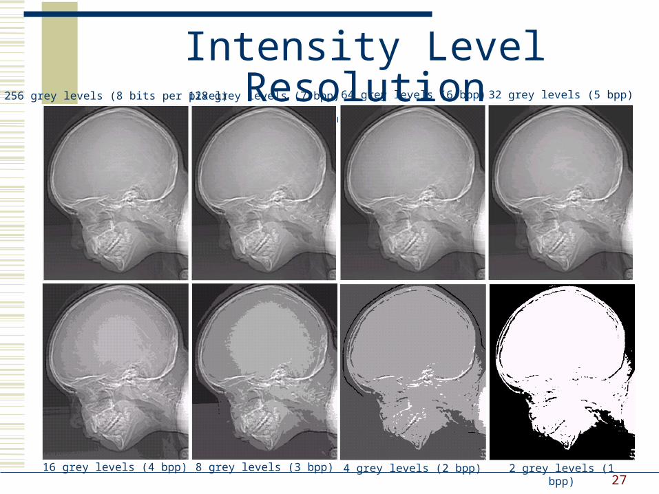
Intensity Level Resolution128 grey levels (7 bpp) 64 grey levels (6 bpp) 32 grey levels (5 bpp)
16 grey levels (4 bpp) 8 grey levels (3 bpp) 4 grey levels (2 bpp) 2 grey levels (1 bpp)
256 grey levels (8 bits per pixel)
28
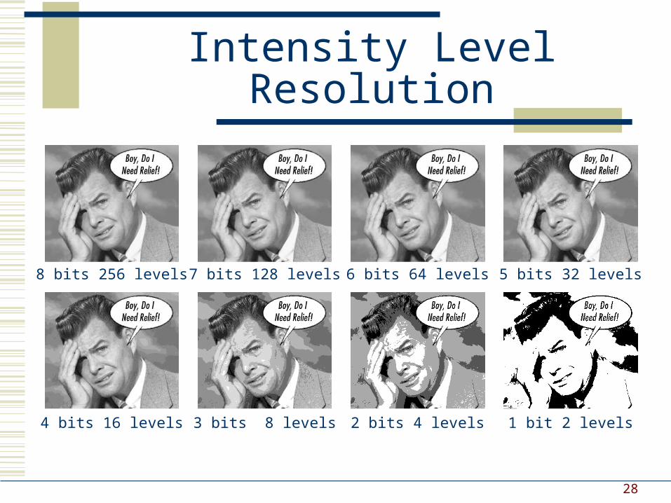
Intensity Level Resolution
8 bits 256 levels 7 bits 128 levels 6 bits 64 levels 5 bits 32 levels
4 bits 16 levels 3 bits 8 levels 2 bits 4 levels 1 bit 2 levels

29
Resolution: How much is enough?
How many samples and gray levels are required for a good approximation? Quality of an image depends on number of pixels and gray-
level number The more these parameters are increased, the closer the
digitized array approximates the original image But: Storage & processing requirements increase rapidly as a
function of N, M, and k

30
Resolution: How much is enough?
Depends on what is in the image and what you would like to do with it
The picture on the right is fine for counting the number of cars, but not for reading the number plate

31
Image Interpolation
Image resizing
Three methods
32
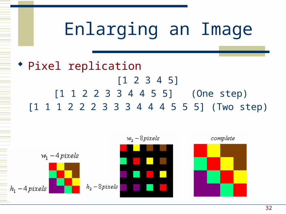
Enlarging an Image
Pixel replication[1 2 3 4 5]
[1 1 2 2 3 3 4 4 5 5] (One step)
[1 1 1 2 2 2 3 3 3 4 4 4 5 5 5] (Two step)

33
Enlarging an Image
Example: zoom this image 4x to get this image.
Example: zoom this image 4x to get this image.
Start with a blank image 4 times the linear dimensions of the original.
Start with a blank image 4 times the linear dimensions of the original.
Fill in every 4th pixel in every 4th row with the original pixel values.
Fill in every 4th pixel in every 4th row with the original pixel values.
…
…
…
…
…
…...

34
Enlarging an Image
Detail showing every 4th pixel in every 4th row with the original pixel values.
Detail showing every 4th pixel in every 4th row with the original pixel values.
…
…
…
…
…
…

35
Enlarging an Image
Replicate the valuesReplicate the values

36
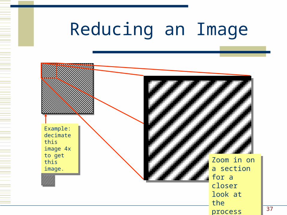
Reducing an Image
Example: decimate this image 4x to get this image.
Example: decimate this image 4x to get this image.
Decimation by a factor of n: take every nth pixel in every nth row
Pixel Decimation
37
Reducing an Image
Example: decimate this image 4x to get this image.
Example: decimate this image 4x to get this image.
Zoom in on a section for a closer look at the process
Zoom in on a section for a closer look at the process

38
Reducing an Image
Example: decimate this image 4x to get this image.
Example: decimate this image 4x to get this image.
Keep every 4th pixel in every 4th row
Keep every 4th pixel in every 4th row

39
Reducing an Image
Example: decimate this image 4x to get this image.
Example: decimate this image 4x to get this image.
ignore all the others
ignore all the others

40
Reducing an Image
Example: decimate this image 4x to get this image.
Example: decimate this image 4x to get this image.
Copy them into a new image.
Copy them into a new image.

41
Nearest Neighbor Interpolation
The “Nearest Neighbor” algorithm is a generalization of pixel replication and decimation.
It also includes fractional resizing, i.e. resizing an image so that it has p/q of the pixels per row and p/q of the rows in the original. (p and q are both integers.)

42
Nearest Neighbor Interpolation
Zoom in on a section for a closer look at the process
Zoom in on a section for a closer look at the process
Example: resize to 3/7 of the original
Example: resize to 3/7 of the original

43
Nearest Neighbor Interpolation
Zoom in for a better look
Zoom in for a better look
3/7 resize 3/7 resize

44
Nearest Neighbor Interpolation
Outlined in blue: 7x7 pixel squares
Outlined in blue: 7x7 pixel squares
3/7 resize 3/7 resize

45
Nearest Neighbor Interpolation
In yellow: 3 pixels for every 7 rows, 3 pixels for every 7 cols.
In yellow: 3 pixels for every 7 rows, 3 pixels for every 7 cols.
3/7 resize 3/7 resize

46
Nearest Neighbor Interpolation
Keep the highlighted pixels…
Keep the highlighted pixels…
3/7 resize 3/7 resize

47
Nearest Neighbor Interpolation
… don’t keep the others.
… don’t keep the others.
3/7 resize 3/7 resize

48
Nearest Neighbor Interpolation
3/7 resize 3/7 resize
Copy them into a new image.
Copy them into a new image.

49
Nearest Neighbor Interpolation
3/7 resize 3/7 resize
Copy them into a new image.
Copy them into a new image.

50
Nearest Neighbor Interpolation
3/7 times the linear dimensions of the original
3/7 times the linear dimensions of the original

51
Nearest Neighbor Interpolation
Resize to 3/7 of the original dims.
Resize to 3/7 of the original dims.
Original image
Original image
Detail of resized image
Detail of resized image

52
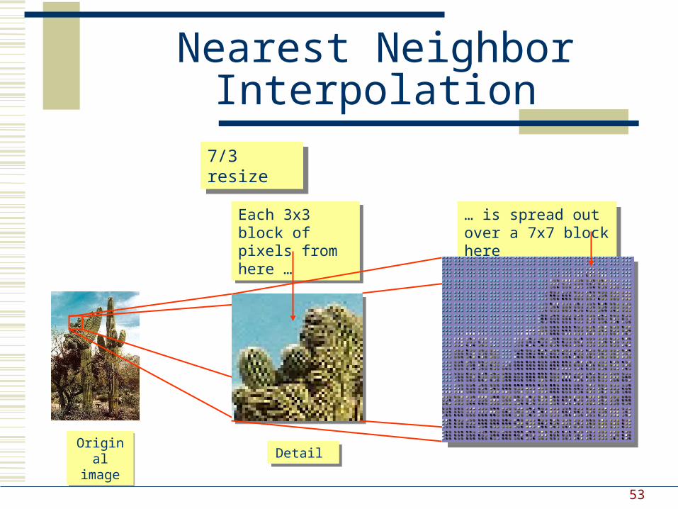
Nearest Neighbor Interpolation
Original image
Original image
Pixels spread out for a 7/3 resize …
Pixels spread out for a 7/3 resize …
… then filled in.… then filled in.
7/3 resize 7/3 resize
53
Nearest Neighbor Interpolation
7/3 resize 7/3 resize
Detail Detail
Each 3x3 block of pixels from here …
Each 3x3 block of pixels from here …
… is spread out over a 7x7 block here
… is spread out over a 7x7 block here
Original image
Original image

54
Nearest Neighbor Interpolation
3x3 blocks distributed over 7x7 blocks
3x3 blocks distributed over 7x7 blocks
7/3 resize 7/3 resize

55
Nearest Neighbor Interpolation
Empty pixels filled with color from non-empty pixel
Empty pixels filled with color from non-empty pixel
7/3 resize 7/3 resize

56
Nearest Neighbor Interpolation7/3 resize 7/3 resize
Empty pixels filled with color from non-empty pixel
Empty pixels filled with color from non-empty pixel

Nearest Neighbor Interpolation
Original image
Original image
7/3 resized 7/3 resized

58
Image Interpolation
Nearest neighbour interpolation Simple but produces undesired artefacts
Bilinear Interpolation Contribution from 4 neighbors
Bicubic Interpolation Contribution from 16 neighbors

Interpolation: Comparison
We’ll enlarge this image by a factor of 4 …
We’ll enlarge this image by a factor of 4 …
… via bilinear interpolation and compare it to a nearest neighbor enlargement.
… via bilinear interpolation and compare it to a nearest neighbor enlargement.

Interpolation: Comparison
To better see what happens, we’ll look at the parrot’s eye.
To better see what happens, we’ll look at the parrot’s eye.
Original Image
Original Image

Interpolation: Comparison
Pixel replication
Pixel replication
Bilinear interpolation
Bilinear interpolation

Interpolation: Comparison
Pixel replication
Pixel replication
Bilinear interpolation
Bilinear interpolation
63
Steganography
The science of writing hidden messages in such a way that no one, apart from the sender and intended recipient, suspects the existence of
the message

64
Steganography
Before Moving On …. Recall – Logical Shift Operators
Logical left shift one bit Logical right shift one bit

SteganographySteganography
8-bit Image 6-bit ImageTwo
leas
t sig
nific
ant b
its a
re 0
If an image is quantized, say from 8 bits to 6 bits and redisplayed it can be all but impossible to tell the difference between the two.

66
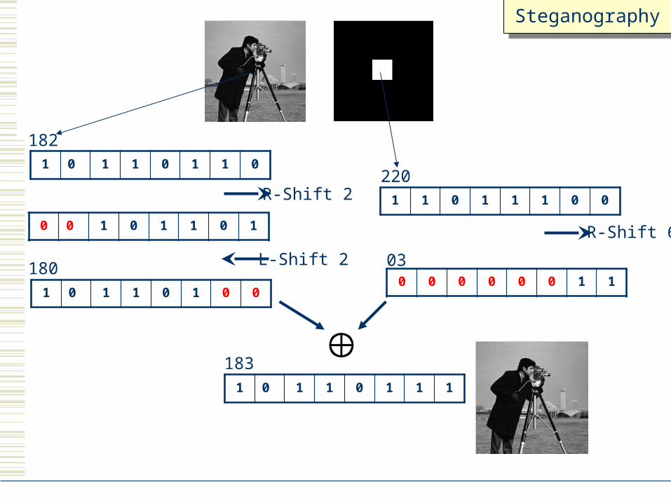
Steganography
That other information could be a message, perhaps encrypted, or even another image.
If the 6-bit version is displayed as an 8-bit image then the 8-bit pixels all have zeros in the lower 2 bits:
00bb bb b b
b = 0 or 1 always 0
This introduces the possibility of encoding other information in the low-order bits.
Image 2
R-Shift 6
Image Out
Image 1
R-Shift 2
L-Shift 2
X-Shift n = logical left or right shift by n bits.
logical OR
0 0 1 0 1 1 0 1
1 0 1 1 0 1 0 0
180
1 1 0 1 1 1 0 0
220
0 0 0 0 0 0 1 103
1 0 1 1 0 1 1 1
183
1 0 1 1 0 1 1 0
182
R-Shift 2
L-Shift 2
SteganographySteganography
R-Shift 6

1 0 1 1 0 1 1 1
183
SteganographySteganography
L-Shift 6
1 1 0 0 0 0 0 0
192
Extracted Second Image
How
to g
et th
e se
cond
imag
eH
ow to
get
the
seco
nd im
age

0 0 1 0 1 1 0 1
1 0 1 1 0 1 0 0
180
0 0 0 0 0 0 1 1
03
0 0 0 0 0 0 1 103
1 0 1 1 0 1 1 1
183
1 0 1 1 0 1 1 0
182
R-Shift 2
L-Shift 2
SteganographySteganography
R-Shift 6
If we have only 4 colors (2-bits) and we put them in the lower order bits
If we have only 4 colors (2-bits) and we put them in the lower order bits
No need to shift rightNo need to shift right
What would you do to get back original data?
What would you do to get back original data?

70
Steganography
8-bit-per-band, 3-band, “original” image
8-bit-per-band, 3-band, “original” image
71
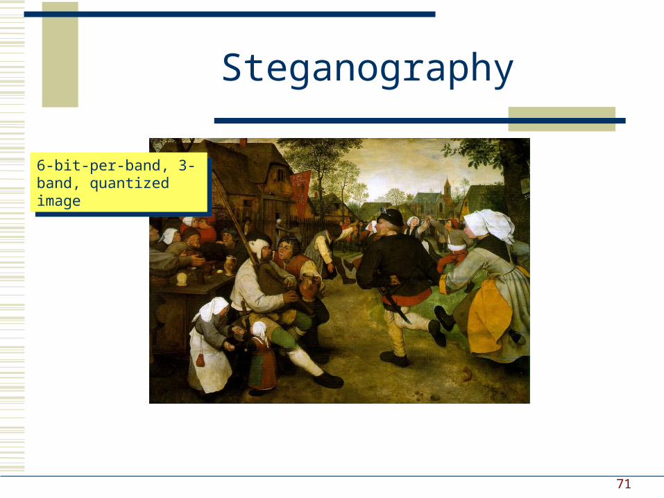
Steganography
6-bit-per-band, 3-band, quantized image
6-bit-per-band, 3-band, quantized image

72
Steganography
The histograms of the two versions indicate which is which. If the 6-bit version is displayed as an 8-bit image it has only pixels with values 0, 4, 8, … , 252.
green-band histogram of 8-bit image green-band histogram of 6-bit image

73
Steganography
The second image is invisible because the value of each pixel is between 0 and 3. For any given pixel, its value is added to the to the collocated pixel in the first image that has a value from the set {0, 4, 8, … , 252}. The 2nd image is noise on the 1st.

74
Steganography
To recover the second image (which is 2 bits per pixel per band) simply left shift the combined image by 6 bits.
L-S
hift
6
?

75
Steganography
To recover the second image (which is 2 bits per pixel per band) simply left shift the combined image by 6 bits.
L-S
hift
6
image

76
Steganography
Images 1 and 2 each have 4-bits per pixel when combined.
Images 1 and 2 each have 4-bits per pixel when combined.
This is so effective that two 4-bit-per-pixel images can be superimposed with only the image in the high-order bits visible. Both images contain the same amount of information but the image in the low-order bits is effectively invisible
Image 2
R-Shift 4
Image Out
Image 1
R-Shift 4
L-Shift 4

77
Steganography
Original ImageOriginal Image

78
Steganography
Image quantized to 4-bits per pixel.
Image quantized to 4-bits per pixel.

79
Steganography
Image 1 in upper 4-bits. Image 2 in lower 4-bits.
Image 1 in upper 4-bits. Image 2 in lower 4-bits.

80
Steganography
Extracted Image

81
Steganography
http://mozaiq.org/encrypt/

82
Relationships between pixels
Neighbors of pixel are the pixels that are adjacent pixels of an identified pixel
x-1 x+1x
y-1
y+1
y

83
4- Neighbors of a Pixel –N4(p)
x-1 x+1x
y-1
y+1
y
(x-1,y), (x+1,y), (x, y-1), (x, y+1)
Wha
t are
the
coor
dina
tes
of
each
of
the
blue
pix
els
Wha
t are
the
coor
dina
tes
of
each
of
the
blue
pix
els

84
Diagonal Neighbors of a Pixel –ND(p)
x-1 x+1x
y-1
y+1
y
(x-1,y-1), (x+1,y-1), (x-1, y+1), (x+1, y+1)

85
8- Neighbors of a Pixel –N8(p)
x-1 x+1x
y-1
y-1
y
(x-1,y), (x+1,y), (x, y-1), (x, y+1)
(x-1,y-1), (x+1,y-1), (x-1, y+1), (x+1, y+1)
8 4( ) ( ) ( )DN p N p N p

86
Determine different regions in the image

87
Connectivity
Establishing boundaries of objects and components in
an image
Group the same region by assumption that the pixels
being the same color or equal intensity
Two pixels p & q are connected if They are adjacent in some sense If their gray levels satisfy a specified criterion of similarity

88
Connectivity
V: Set of gray levels used to define the criterion of similarity
4-connectivity4-connectivity
If gray level 4( , ) , ( )p q V and q N p
Set of gray levels V = {1}Set of gray levels V = {1}

89
Connectivity
V: Set of gray levels used to define the criterion of similarity
8-connectivity8-connectivity
If gray level 8( , ) , ( )p q V and q N p
Set of gray levels V = {1}Set of gray levels V = {1}
90
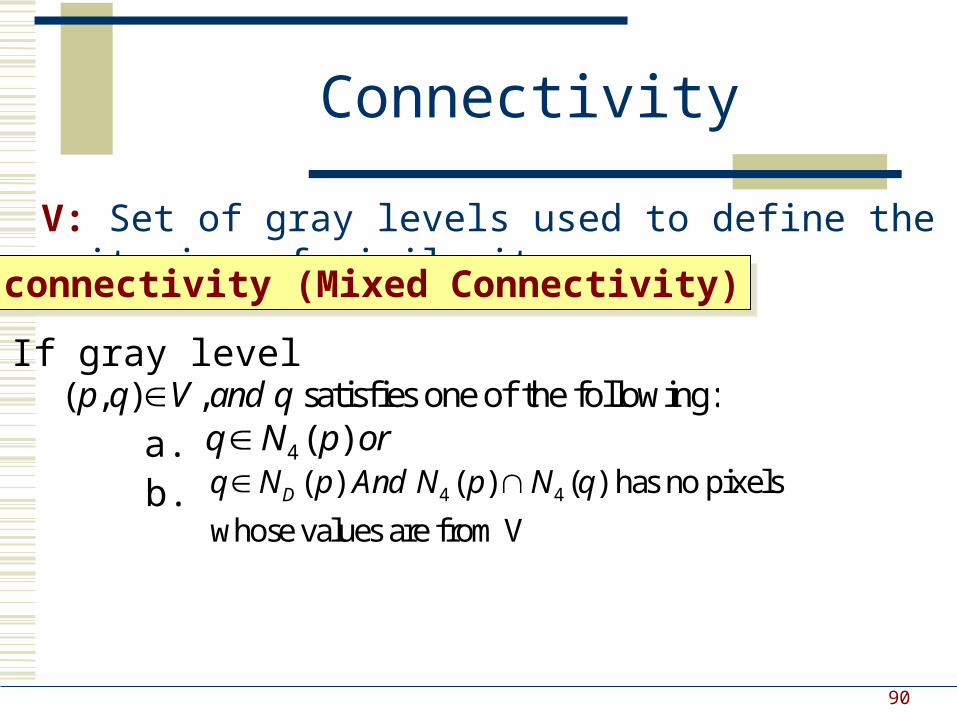
Connectivity
V: Set of gray levels used to define the criterion of similarity
m-connectivity (Mixed Connectivity)m-connectivity (Mixed Connectivity)
If gray level( , ) , satisfies one of the following:p q V and q
4 ( )q N p or4 4( ) ( ) ( ) has no pixels
whose values are from VDq N p And N p N q
a.b.
91
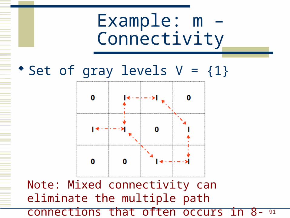
Example: m – Connectivity
Set of gray levels V = {1}
Note: Mixed connectivity can eliminate the multiple path connections that often occurs in 8-connectivity

92
Paths
Path: Let coordinates of pixel p: (x, y), and of pixel q:
(s, t)
A path from p to q is a sequence of distinct pixels with
coordinates: (x0, y0), (x1, y1), ......, (xn,yn)
where (x0, y0) = (x, y) & (xn,yn) = (s, t), and (xi,yi) is adjacent to
(xi-1,yi-1) 1≤i ≤n

93
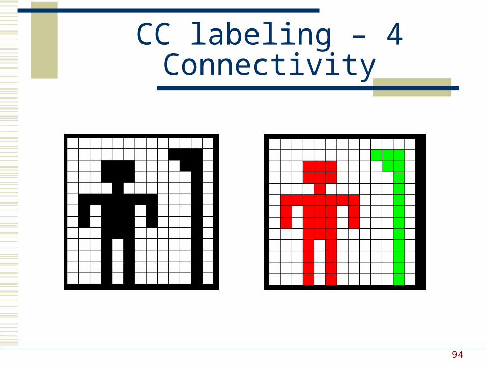
CC labeling – 4 Connectivity Process the image from left to
right, top to bottom:1.) If the next pixel to process is 1 i.) If only one of its neighbors
(top or left) is 1, copy its label.
ii.) If both are 1 and have the same label, copy it.
iii.) If they have different labels Copy the label from the left. Update the equivalence table.
iv.) Otherwise, assign a new label.
Re-label with the smallest of equivalentlabels
Pass 1
Pass 2
94
CC labeling – 4 Connectivity

95
CC labeling – 4 Connectivity

96
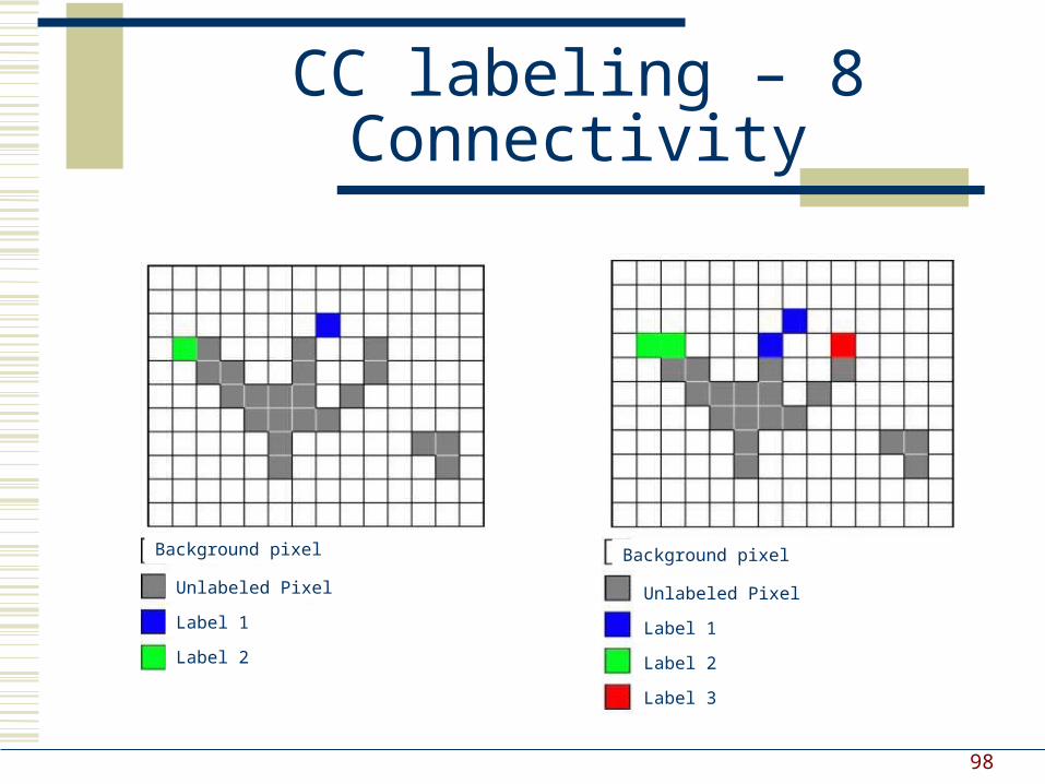
CC labeling – 8 Connectivity
Same algorithm but examine also the upper diagonal neighbors of p
Same algorithm but examine also the upper diagonal neighbors of p

97
CC labeling – 8 Connectivity
Background pixel
Unlabeled Pixel
Background pixel
Unlabeled Pixel
Label 1
98
CC labeling – 8 Connectivity
Background pixel
Unlabeled Pixel
Label 1
Label 2
Background pixel
Unlabeled Pixel
Label 1
Label 2
Label 3

99
CC labeling – 8 Connectivity
Background pixel
Unlabeled Pixel
Label 1
Label 2
Label 3
Background pixel
Unlabeled Pixel
Label 1
Label 2
Label 3

100
CC labeling – 8 Connectivity
Background pixel
Label 1
Label 2
Label 3
Unlabeled pixel
Background pixel
Label 1
Label 2
Label 3
Unlabeled pixel

101
CC labeling – 8 Connectivity
Background pixel
Label 1
Label 2
Label 3
Unlabeled pixel
Label 4
Background pixel
Label 1
Label 2
Label 3
Unlabeled pixel
Label 4

102
Distance Metrics
Let pixels p, q and z have coordinates (x,y), (s,t) and (u,v) respectively.
D is a distance function or metric if D(p,q) ≥ 0 and D(p,q) = 0 iff p = q and D(p,q) = D(q,p) and D(p,z) ≤ D(p,q) + D(q,z)

103
City block distance (D4 distance)
4 ( , )D p q x s y t
Diamond with center at (x,y) D4 = 1 are the 4 neighbors of
pixel p(x,y)

104
Chessboard distance (D8 distance)
8 ( , ) max( , )D p q x s y t
Square centered at p(x,y) D8 = 1 are the 8 neighbors of
pixel p(x,y)

105
Euclidean Distance
2 2( , ) ( ) ( )eD p q x s y t
A circle with radius r centered at (x,y)
p(x,y)
q(s,t)
r

106
Arithmetic Operations
Carried out between corresponding pixel pairs
( , ) ( , ) ( , )s x y f x y g x y
( , ) ( , ) ( , )d x y f x y g x y ( , ) ( , ) ( , )p x y f x y g x y
( , ) ( , ) ( , )d x y f x y g x y

107
Arithmetic Operations
Conversion to range 0 – 255 Difference of two 8-bit images: -255 to 255 Sum of two 8-bit images: 0 to 510 Solution?
Set all values < 0 to 0
Set all values > 255 to 255
Full range of arithmetic operation not captured

108
Arithmetic Operations
First perform the operation
Then perform
min( )mf f f
Creates an image whose minimum value is 0
max( )s m mf K f f
Creates a scaled image fs with values in the range
[0 K]

109
Logical Operations (Binary Images)

Reading Assignment
2.6.1 Array versus Matrix Operations
2.6.2 Linear versus Non-Linear Operations
Readings from Book (3rd Edn.)
2.4 Image Sampling & Quantization*
2.5 Basic Relationships between Pixels
*Discussion related to figures 2.22 and 2.23 has not been covered

112
Acknowledgements
Digital Image Processing”, Rafael C. Gonzalez & Richard E. Woods, Addison-Wesley, 2002 Peters, Richard Alan, II, Lectures on Image Processing, Vanderbilt University, Nashville, TN,
April 2008 Brian Mac Namee, Digitial Image Processing, School of Computing, Dublin Institute of
Technology Computer Vision for Computer Graphics, Mark Borg
Mat
eria
l in
thes
e sl
ides
has
bee
n ta
ken
from
the
foll
owin
g re
sour
ces