Illiquidityandstockreturns: cross-sectionandtime ...mkearns/finread/amihud.pdf ·...

Journal of Financial Markets 5 (2002) 31–56

Illiquidity and stock returns:cross-section and time-series effects$

Yakov Amihud*

Stern School of Business, New York University, New York, NY 10012, USA

Abstract

This paper shows that over time, expected market illiquidity positively affects ex antestock excess return, suggesting that expected stock excess return partly represents anilliquidity premium. This complements the cross-sectional positive return–illiquidity

relationship. Also, stock returns are negatively related over time to contemporaneousunexpected illiquidity. The illiquidity measure here is the average across stocks ofthe daily ratio of absolute stock return to dollar volume, which is easily obtained from

daily stock data for long time series in most stock markets. Illiquidity affects morestrongly small firm stocks, thus explaining time series variations in their premiums overtime. r 2002 Elsevier Science B.V. All rights reserved.

JEL classificaion: G12

Keywords: Liquidity and asset pricing; Liquidity premium

1. Introduction

The hypothesis on the relationship between stock return and stock liquidityis that return increases in illiquidity, as proposed by Amihud and Mendelson(1986). The positive return–illiquidity relationship has been examined across

$I thank Haim Mendelson for valuable suggestions and Viral Acharya for competent research

assistance and comments. Helpful comments were received from Michael Brennan, Martin Gruber,

Richard Roll, two anonymous referees and Avanidhar Subrahmanyam (the editor).

*Tel.: +1-212-998-0720; fax: +1-212-995-4220.

E-mail address: [email protected] (Y. Amihud).

1386-4181/02/$ - see front matter r 2002 Elsevier Science B.V. All rights reserved.

PII: S 1 3 8 6 - 4 1 8 1 ( 0 1 ) 0 0 0 2 4 - 6

stocks in a number of studies. This study examines this relationship over time.It proposes that over time, the ex ante stock excess return is increasing in theexpected illiquidity of the stock market.The illiquidity measure employed here, called ILLIQ; is the daily ratio of

absolute stock return to its dollar volume, averaged over some period. It can beinterpreted as the daily price response associated with one dollar of tradingvolume, thus serving as a rough measure of price impact. There are finer andbetter measures of illiquidity, such as the bid ask spread (quoted or effective),transaction-by-transaction market impact or the probability of information-based trading. These measures, however, require a lot of microstructure datathat are not available in many stock markets. And, even when available,the data do not cover very long periods of time. The measure used here enablesto construct long time series of illiquidity that are necessary to test the effectsover time of illiquidity on ex ante and contemporaneous stock excess return.This would be very hard to do with the finer microstructure measures ofilliquidity.The results show that both across stocks and over time, expected

stock returns are an increasing function of expected illiquidity. Across NYSEstocks during 1964–1997, ILLIQ has a positive and highly significant effecton expected return. The new tests here are on the effects over time of marketilliquidity on market excess return (stock return in excess of the Treasurybill rate). Stock excess return, traditionally called ‘‘risk premium’’, has beenconsidered a compensation for risk. This paper proposes that expectedstock excess return also reflects compensation for expected market illiquidity,and is thus an increasing function of expected market illiquidity. The resultsare consistent with this hypothesis. In addition, unexpected market illiquiditylowers contemporaneous stock prices. This is because higher realizedilliquidity raises expected illiquidity that in turn raises stock expectedreturns and lowers stock prices (assuming no relation between corporatecash flows and market liquidity). This hypothesis too is supported by theresults. These illiquidity effects are shown to be stronger for small firms’stocks. This suggests that variations over time in the ‘‘size effect’’Fthe excessreturn on small firms’ stocksFare related to changes in market liquidityover time.The paper proceeds as follows. Section 2 introduces the illiquidity measure

used in this study and employs it in cross-section estimates of expected stockreturns as a function of stock illiquidity and other variables. Section 3 presentsthe time-series tests of the effect of the same measure of illiquidity on ex antestock excess returns. The section includes tests of the effect of expected andunexpected illiquidity, the effects of these variables for different firm-sizeportfolios and the effects of expected illiquidity together with the effects ofother variablesFbonds’ term and default yield premiumsFthat predict stockreturns. Section 4 offers concluding remarks.

Y. Amihud / Journal of Financial Markets 5 (2002) 31–5632

2. Cross-section relationship between illiquidity and stock return

2.1. Measures of illiquidity

Liquidity is an elusive concept. It is not observed directly but rather has anumber of aspects that cannot be captured in a single measure.1 Illiquidityreflects the impact of order flow on priceFthe discount that a seller concedes orthe premium that a buyer pays when executing a market orderFthat resultsfrom adverse selection costs and inventory costs (Amihud and Mendelson, 1980;Glosten and Milgrom, 1985). For standard-size transactions, the price impact isthe bid–ask spread, whereas larger excess demand induces a greater impact onprices (Kraus and Stoll, 1972; Keim and Madhavan, 1996), reflecting a likelyaction of informed traders (see Easley and O’Hara, 1987). Kyle (1985) proposedthat because market makers cannot distinguish between order flow that isgenerated by informed traders and by liquidity (noise) traders, they set pricesthat are an increasing function of the imbalance in the order flow which mayindicate informed trading. This creates a positive relationship between the orderflow or transaction volume and price change, commonly called the price impact.These measures of illiquidity are employed in studies that examine the cross-

section effect of illiquidity on expected stock returns. Amihud and Mendelson(1986) and Eleswarapu (1997) found a significant positive effect of quotedbid–ask spreads on stock returns (risk-adjusted).2 Chalmers and Kadlec (1998)used the amortized effective spread as a measure of liquidity, obtained fromquotes and subsequent transactions, and found that it positively affects stockreturns.3 Brennan and Subrahmanyam (1996) measured stock illiquidity byprice impact, measured as the price response to signed order flow (order size),and by the fixed cost of trading, using intra-day continuous data ontransactions and quotes.4 They found that these measures of illiquidity

1See discussion in Amihud and Mendelson (1991b).2Amihud and Mendelson (1986) study is on NYSE/AMEX stocks, 1961–1980, and Eleswarapu’s

(1997) study is on Nasdaq stocks, 1974–1990. Bond yields are also found to be increasing in the

bid–ask spread, after controlling for maturity and risk. See Amihud and Mendelson (1991a) and

Kamara (1994).3The effective spread is the absolute difference between the mid-point of the quoted bid–ask

spread and the transaction price that follows, classified as being a buy or sell transaction. The

spread is divided by the stock’s holding period, obtained from the turnover rate on the stock, to

obtain the amortized spread.4This measure, based on Kyle’s (1985) model, is estimated by the methods proposed by Glosten

and Harris (1988) and Hasbrouck (1991). Basically, it is the slope coefficient in a regression of

transaction-by-transaction price changes on the signed order size, where orders are classified into

‘‘buy’’ or ‘‘sell’’ by the proximity of the transaction price to the preceding bid and ask quotes.

Adjustments are made for prior information (on price changes and order size) and fixed order

placement costs.

Y. Amihud / Journal of Financial Markets 5 (2002) 31–56 33

positively affect stock returns. Easley et al. (1999) introduced a new measure ofmicrostructure risk, the probability of information-based trading, that reflectsthe adverse selection cost resulting from asymmetric information betweentraders, as well as the risk that the stock price can deviate from its full-information value. This measure is estimated from intra-daily transaction data.They found that across stocks, the probability of information-based tradinghas a large positive and significant effect on stock returns.These fine measures of illiquidity require for their calculation microstructure

data on transactions and quotes that are unavailable in most markets aroundthe world for long time periods of time. In contrast, the illiquidity measureused in this study is calculated from daily data on returns and volume that arereadily available over long periods of time for most markets. Therefore, while itis more coarse and less accurate, it is readily available for the study of the timeseries effects of liquidity.Stock illiquidity is defined here as the average ratio of the daily absolute

return to the (dollar) trading volume on that day, jRiyd j=VOLDiyd : Riyd is thereturn on stock i on day d of year y and VOLDiyd is the respective daily volumein dollars. This ratio gives the absolute (percentage) price change per dollar ofdaily trading volume, or the daily price impact of the order flow. This followsKyle’s concept of illiquidityFthe response of price to order flowFand Silber’s(1975) measure of thinness, defined as the ratio of absolute price change toabsolute excess demand for trading.The cross-sectional study employs for each stock i the annual average

ILLIQiy ¼ 1=Diy

XDiy

t¼1

jRiyd j=VOLDivyd ; ð1Þ

where Diy is the number of days for which data are available for stock i in yeary: This illiquidity measure is strongly related to the liquidity ratio known as theAmivest measure, the ratio of the sum of the daily volume to the sum of theabsolute return (e.g., Cooper et al., 1985; Khan and Baker, 1993). Amihud et al.(1997) and Berkman and Eleswarapu (1998) used the liquidity ratio to studythe effect of changes in liquidity on the values of stocks that were subject tochanges in their trading methods. The liquidity ratio, however, does not havethe intuitive interpretation of measuring the average daily association betweena unit of volume and the price change, as does ILLIQ:5

ILLIQ should be positively related to variables that measure illiquidity frommicrostructure data. Brennan and Subrahmanyam (1996) used two measures

5Another interpretation of ILLIQ is related to disagreement between traders about new

information, following Harris and Raviv (1993). When investors agree about the implication of

news, the stock price changes without trading while disagreement induces increase in trading

volume. Thus, ILLIQ can also be interpreted as a measure of consensus belief among investors

about new information.


of illiquidity, obtained from data on inraday transactions and quotes: Kyle’s(1985) l; the price impact measure, and c; the fixed-cost component related tothe bid–ask spread. The estimates are done by the method of Glosten andHarris (1988). Using estimates6 of these variables for 1984, the following cross-sectional regression was estimated:

ILLIQi ¼ �292þ 247:9li þ 49:2ci

ðt ¼Þ ð12:25Þ ð13:78Þ ð17:33Þ R2 ¼ 0:30:

These results show that ILLIQ is positively and strongly related tomicrostructure estimates of illiquidity.Size, or the market value of the stock, is also related to liquidity since a

larger stock issue has smaller price impact for a given order flow and a smallerbid–ask spread. Stock expected returns are negatively related to size (Banz,1981; Reinganum, 1981; Fama and French, 1992), which is consistent with itbeing a proxy for liquidity (Amihud and Mendelson, 1986).7 The negativereturn-size relationship may also result from the size variable being related to afunction of the reciprocal of expected return (Berk, 1995).There are other measures of liquidity that use data on volume. Brennan

et al. (1998) found that the stock (dollar) volume has a significant negativeeffect on the cross-section of stock returns and it subsumes the negativeeffect of size. Another related measure is turnover, the ratio of tradingvolume to the number of shares outstanding. By Amihud and Mendelson(1986), turnover is negatively related to illiquidity costs, and Atkinsand Dyl (1997) found a strong positive relationship across stocks betweenthe bid–ask spread and the reciprocal of the turnover ratio that measuresholding period. A number of studies find that cross-sectionally, stockreturns are decreasing in stock turnover, which is consistent with anegative relationship between liquidity and expected return (Haugenand Baker, 1996; Datar et al., 1998; Hu, 1997a; Rouwenhorst, 1998; Chordiaet al., 2001).These measures of liquidity as well as the illiquidity measure presented in this

study can be regarded as empirical proxies that measure different aspects ofilliquidity. It is doubtful that there is one single measure that captures all itsaspects.

6 I thank M. Bennan and Avanidhar Subrahmnaym for kindly providing these estimates. The

estimated variables are multiplied here by 103. Outliers at the upper and lower 1% tails of these

variables and of ILLIQ are discarded (see Brennan and Subrahmanyam, 1996).7Barry and Brown (1984) propose that the higher return on small firms’ stock is compensation

for less information available on small firms that have been listed for a shorter period of time. This

is consistent with the illiquidity explanation of the small firm effect since illiquidity costs are

increasing in the asymmetry of information between traders (see Glosten and Milgrom, 1985; Kyle,

1985).


2.2. Empirical methodology

The effect of illiquidity on stock return is examined for stocks traded in theNew York Stock Exchange (NYSE) in the years 1963–1997, using data fromdaily and monthly databases of CRSP (Center for Research of Securities Prices ofthe University of Chicago). Tests are confined to NYSE-traded stocks to avoidthe effects of differences in market microstructures.8 The test procedure followsthe usual Fama and MacBeth (1973) method. A cross-section model is estimatedfor each month m ¼ 1; 2;y; 12 in year y; y ¼ 1964; 1965;y; 1997 (a total of 408months), where monthly stock returns are a function of stock characteristics:

Rimy ¼ komy þXJ

j¼1

kjmyXji;y�1 þUimy: ð2Þ

Rimy is the return on stock i in month m of year y; with returns being adjusted forstock delistings to avoid survivorship bias, following Shumway (1997).9 Xji;y�1 ischaracteristic j of stock i; estimated from data in year y� 1 and known to investorsat the beginning of year y; during which they make their investment decisions. Thecoefficients kjmy measure the effects of stock characteristics on expected return, andUimy are the residuals. The monthly regressions of model (2) over the period1964–1997 produce 408 estimates of each coefficient kjmy; j ¼ 0; 1; 2;y; J: Thesemonthly estimates are averaged and tests of statistical significance are performed.Stocks are admitted to the cross-sectional estimation procedure in month m of

year y if they have a return for that month and they satisfy the following criteria:

(i) The stock has return and volume data for more than 200 days during yeary� 1: This makes the estimated parameters more reliable. Also, the stock mustbe listed at the end of year y� 1:(ii) The stock price is greater than $5 at the end of year y� 1: Returns on

low-price stocks are greatly affected by the minimum tick of $1/8, which addsnoise to the estimations.10

8See Reinganum (1990) on the effects of the differences in microstructure between the NASDAQ

and the NYSE on stock returns, after adjusting for size and risk. In addition, volume figures on the

NASDAQ have a different meaning than those on the NYSE, because trading on the NASDAQ is

done almost entirely through market makers, whereas on the NYSE most trading is done directly

between buying and selling investors. This results in artificially higher volume figures on NASDAQ.9Specifically, the last return used is either the last return available on CRSP, or the

delisting return, if available. Naturally, a last return for the stock of �100% is included in the

study. A return of –30% is assigned if the deletion reason is coded by 500 (reason unavailable), 520

(went to OTC), 551–573 and 580 (various reasons), 574 (bankruptcy) and 584 (does not meet

exchange financial guidelines). Shumway (1997) obtains that –30% is the average delisting return,

examining the OTC returns of delisted stocks.10See discussion on the minimum tick and its effects in Harris (1994). The benchmark of $5 was

used in 1992 by the NYSE when it reduced the minimum tick. Also, the conventional term of

‘‘penny stocks’’ applies to stocks whose price is below $5.


(iii) The stock has data on market capitalization at the end of year y� 1 inthe CRSP database. This excludes derivative securities like ADRs of foreignstocks and scores and primes.(iv) Outliers are eliminatedFstocks whose estimated ILLIQiy in year y� 1

is at the highest or lowest 1% tails of the distribution (after satisfying criteria(i)–(iii)).

There are between 1061 and 2291 stocks that satisfy these four conditionsand are included in the cross-section estimations.

2.3. Stock characteristics

2.3.1. Liquidity variablesThe measure of liquidity is ILLIQiy that is calculated for each stock i in year

y from daily data as in (1) above (multiplied by 106). The average marketilliquidity across stocks in each year is calculated as

AILLIQy ¼ 1=Ny

XNy

t¼1

ILLIQiy; ð3Þ

where Ny is the number of stocks in year y. (The stocks that are usedto calculate the average illiquidity are those that satisfy conditions (i)–(iv)above.) Since average illiquidity varies considerably over the years, ILLIQiy isreplaced in the estimation of the cross-section model (2) by its mean-adjustedvalue

ILLIQMAiy ¼ ILLIQiy=AILLIQy: ð4Þ

The cross-sectional model (2) also includes SIZEiy; the market value ofstock i at the end of year y; as given by CRSP. As discussed above, SIZEmay also be a proxy for liquidity. Table 1 presents estimated statistics of ILLIQand SIZE: In each year, the annual mean, standard deviation acrossstocks and skewness are calculated for stocks admitted to thesample, and then these annual statistics are averaged over the 34 years.The correlations between the variables are calculated in each year acrossstocks and then the yearly correlation coefficients are averaged over theyears. As expected, ILLIQiy is negatively correlated with size:CorrðILLIQiy; ln SIZEiyÞ ¼ �0:614:

2.3.2. Risk variablesModel (2) includes BETAiy as a measure of risk, calculated as follows. At the

end of each year y; stocks are ranked by their size (capitalization) and dividedinto ten equal portfolios. (Size serves here as an instrument.) Next, theportfolio return Rpty is calculated as the equally-weighted average of stockreturns in portfolio p on day t in year y: Then, the market model is estimated


for each portfolio p; p ¼ 1; 2;y; 10;

Rpty ¼ apy þ BETApy � RMty þ epty: ð5Þ

RMty is the equally-weighted market return and BETApy is the slopecoefficient, estimated by the Scholes and Williams (1977) method. The betaassigned to stock i; BETAiy; is BETApy of the portfolio in which stock i isincluded. Fama and French (1992), who used similar methodology, suggestedthat the precision of the estimated portfolio beta more than makes up for thefact that not all stocks in the size portfolio have the same beta.11

The stock total risk is SDRETiy; the standard deviation of the daily returnon stock i in year y (multiplied by 102). By the asset pricing models of Levy(1978) and Merton (1987), SDRET is priced since investors’ portfolios areconstrained and therefore not well diversified. However, the tax trading option(due to Constantinides and Scholes, 1980) suggests that stocks with highervolatility should have lower expected return. Also, SDRETiy is included in themodel since ILLIQiy may be construed as a measure of the stock’s risk, giventhat its numerator is the absolute return (which is related to SDRETiy),

Table 1

Statistics on variables

The illiquidity measure, ILLIQiy; is the average for year y of the daily ratio of absolute return to thedollar volume of stock i in year y: SIZEiy is the market capitalization of the stock at the end of theyear given by CRSP, DIVYLDiy; the dividend yield, is the sum of the annual cash dividend dividedby the end-of-year price, SDRETiy is the standard deviation of the stock daily return. Stocks

admitted in each year y have more than 200 days of data for the calculation of the characteristics

and their end-of-year price exceeds $5. Excluded are stocks whose ILLIQiy is at the extreme 1%

upper and lower tails of the distribution.

Each variable is calculated for each stock in each year across stocks admitted to the sample in that

year, and then the mean, standard deviation and skewness are calculated across stocks in each year.

The table presents the means over the 34 years of the annual means, standard deviations and

skewness and the medians of the annual means, as well as the maximum and minimum annual means.

Data include NYSE stocks, 1963–1996.

Variable Mean of

annual

means

Mean of

annual

S.D.

Median of

annual

means

Mean of

annual

skewness

Min.

annual

mean

Max.

annual

mean

ILLIQ 0.337 0.512 0.308 3.095 0.056 0.967

SIZE ($million) 792.6 1,611.5 538.3 5.417 263.1 2,195.2

DIVYLD (%) 4.14 5.48 4.16 5.385 2.43 6.68

SDRET 2.08 0.75 2.07 1.026 1.58 2.83

11The models were re-estimated using betas of individual stocks in lieu of betas of size portfolios.

These betas have an insignificant effect in the cross-section regressions. The results on ILLIQ

remained the same. Also, omitting BETA altogether from the cross-section regression has very little

effect on the results.


although the correlation between ILLIQ and SDRET is low, 0.278.Theoretically, risk and illiquidity are positively related. Stoll (1978) proposedthat the stock illiquidity is positively related to the stock’s risk since the bid–askspread set by a risk-averse market maker is increasing in the stock’s risk.Copeland and Galai (1983) modeled the bid–ask spread as a pair of optionsoffered by the market maker, thus it increases with volatility. Constantinides(1986) proposed that the stock variance positively affects the return thatinvestors require on the stock, since it imposes higher trading costs on themdue to the need to engage more frequently in portfolio rebalancing.

2.3.3. Additional variablesThe cross-sectional model (2) includes the dividend yield for stock i in year y;

DIVYLDiy; calculated as the sum of the dividends during year y divided by theend-of-year price (following Brennan et al., 1998). DIVYLD should have apositive effect on stock return if investors require to be compensated for thehigher tax rate on dividends compared to the tax on capital gains. However,DIVYLD may have a negative effect on return across stocks if it is negativelycorrelated with an unobserved risk factor, that is, stocks with higher dividendare less risky. The coefficient of DIVYLD may also be negative followingRedding’s (1997) suggestion that large investors prefer companies with highliquidity and also prefer receiving dividends.12

Finally, past stock returns were shown to affect their expected returns (seeBrennan et al., 1998). Therefore, the cross-sectional model (2) includes twovariables: R100iy, the return on stock i during the last 100 days of year y; andR100YRiy, the return on stock i over the rest of the period, between thebeginning of the year and 100 days before its end.The model does not include the ratio of book-to-market equity, BE/ME, which

was used by Fama and French (1992) in cross-section asset pricing estimation. Thisstudy employs only NYSE stocks for which BE/ME was found to have no sig-nificant effect (Easley et al., 1999; Loughran, 1997).13 Also, Berk (1995) suggestedthat an estimated relation between expected return and BE/ME is obtained due tothe functional relation between expected return and the market value of equity.

2.4. Cross-section estimation results

In the cross-sectional model (2), stock returns in each month of the year areregressed on stock characteristics that are estimated from data in the previous

12Higher dividend yield may be perceived by investors to provide greater liquidity (ignoring tax

consequences). This is analogous to the findings of Amihud and Mendelson (1991a) that Treasury

notes with higher coupon provide lower yield to maturity.13Loughran (1997) finds that when the month of January is exluded, the effect of BE/ME

becomes insignificant.


year (following the Fama and MacBeth (1973) method). Themodel is estimated for 408 months (34 years), generating 408 sets of co-efficients kjmy;m ¼ 1; 2;y; 12; and y ¼ 1964; 1965;y; 1997: The mean andstandard error of the 408 estimated coefficients kjmy are calculatedfor each stock characteristic j; followed by a t-test of the null hypothesis ofzero mean. Tests are also performed for the means that exclude theJanuary coefficients since by some studies, excluding January makes theeffects of beta, size and the bid–ask spread insignificant (e.g., Keim, 1983;Tinic and West, 1986; Eleswarapu and Reinganum, 1993). Finally, toexamine the stability over time of the effects of the stock characteristics,tests are done separately for two equal subperiods of 204 months (17 years)each.The results, presented in Table 2, strongly support the hypothesis that

illiquidity is priced, consistent with similar results in earlier studies. Thecoefficient of ILLIQMAiy; denoted kILLIQmy; has a mean of 0.162 that isstatistically significant (t ¼ 6:55) and its median is 0.135, close to the mean. Ofthe estimated coefficients, 63.4% (259 of the 408) are positive, a proportionthat is significantly different from 1/2 (the chance proportion). The serialcorrelation of the series kILLIQmy is quite negligible (0.08).The illiquidity effect remains positive and highly significant when January

is excluded: the mean of kILLIQmy is 0.126 with t ¼ 5:30: The illiquidity effect ispositive and significant in each of the two subperiods of 17 years.The effect of BETA is positive, as expected, and significant (the statistical

significance is lower when January is excluded). However, it becomesinsignificant when SIZE is included in the model, since beta is calculated forsize-based portfolios. Past returnsFR100 and R100YRFboth have positiveand significant coefficients.Table 2 also presents estimation results of a model that includes additional

variables. The coefficient of ILLIQMA remains positive and significant forthe entire period, for the non-January months and for each of the twosubperiods. In addition, the coefficient of ln SIZE is negative and significant,although its magnitude and significance is lower in the second subperiod.Size may be a proxy for liquidity, but its negative coefficient may also be dueto it being a proxy for the reciprocal of expected return (Berk, 1995). Therisk variable SDRET has a negative coefficient (as in Amihud and Mendelson,1989), perhaps accounting for the value of the tax trading option. The negativecoefficient of DIVYLD may reflect the effect of an unobserved risk factorthat is negatively correlated with DIVYLD across stocks (less risky companiesmay choose to have higher dividend yield). The negative coefficient ofDIVYLD is also consistent with the hypothesis of Redding (1997) aboutdividend preference by some types of investors. These effects could offset thepositive effect of DIVYLD that results from the higher personal tax ondividends.


Table 2

Cross-section regressions of stock return on illiquidity and other stock characteristicsa

The table presents the means of the coefficients from the monthly cross-sectional regression of stock return on the respective variables. In each month of

year y; y ¼ 1964; 1965;y; 1997; stock returns are regressed cross-sectionally on stock characteristics that are calculated from data in year y� 1: BETAis the slope coefficient from an annual time-series regression of daily return on one of 10 size portfolios on the market return (equally weighted), using

the Scholes and Williams (1977) method. The stock’s BETA is the beta of the size portfolio to which it belongs. The illiquidity measure ILLIQ is the

average over the year of the daily ratio of the stock’s absolute return to its dollar trading volume. ILLIQ is averaged every year across stocks, and

ILLIQMA is the respective mean-adjusted variables, calculated as the ratio of the variable to its annual mean across stocks (thus the means of all years

are 1). ln SIZE is the logarithm of the market capitalization of the stock at the end of the year, SDRET is the standard deviation of the stock daily

return during the year, and DIVYLD is the dividend yield, the sum of the annual cash dividend divided by the end-of-year price. R100 is the stock

return over the last 100 days and R100YR is the return during the period between the beginning of the year and 100 days before its end.

The data include 408 months over 34 years, 1964–1997, (the stock characteristics are calculated for the years 1963–1996). Stocks admitted have more

than 200 days of data for the calculation of the characteristics in year y� 1 and their end-of-year price exceeds $5. Excluded are stocks whose ILLIQ isat the extreme 1% upper and lower tails of the respective distribution for the year.

Variable All months Excl. January 1964–1980 1981–1997 All months Excl. January 1964–1980 1981–1997

Constant �0.364 �0.235 �0.904 0.177 1.922 1.568 2.074 1.770(0.76) (0.50) (1.39) (0.25) (4.06) (3.32) (2.63) (3.35)

BETA 1.183 0.816 1.450 0.917 0.217 0.260 0.297 0.137(2.45) (1.75) (1.83) (1.66) (0.64) (0.79) (0.59) (0.30)

ILLIQMA 0.162 0.126 0.216 0.108 0.112 0.103 0.135 0.088(6.55) (5.30) (4.87) (5.05) (5.39) (4.91) (3.69) (4.56)

R100 1.023 1.514 0.974 1.082 0.888 1.335 0.813 0.962(3.83) (6.17) (2.47) (2.96) (3.70) (6.19) (2.33) (2.92)

R100YR 0.382 0.475 0.485 0.279 0.359 0.439 0.324 0.395(2.98) (3.70) (2.55) (1.59) (3.40) (4.27) (2.04) (2.82)

Ln SIZE �0.134 �0.073 �0.217 �0.051(3.50) (2.00) (3.51) (1.14)

SDRET �0.179 �0.274 �0.136 �0.223(1.90) (2.89) (0.96) (1.77)

DIVYLD �0.048 �0.063 �0.075 �0.021(3.36) (4.28) (2.81) (2.11)

a t-statistics in parentheses.

Y.Amihud/JournalofFinancialMarkets

5(2002)31–56

41

The cross-sectional models are also estimated by the weighted least squaresmethod to account for hetersokedasticity in the residuals of model (2). Theresults14 are qualitatively similar to those using the OLS method. In all models,the coefficient of ILLIQMA is positive and significant for the entire sample,when January is excluded and for each of the two subperiods.

3. The effect over time of market illiquidity on expected stock excess return

The proposition here is that over time, expected market illiquidity positivelyaffects expected stock excess return (the stock return in excess of Treasury billrate). This is consistent with the positive cross-sectional relationship betweenstock return and illiquidity. If investors anticipate higher market illiquidity, theywill price stocks so that they generate higher expected return. This suggests thatstock excess return, traditionally interpreted as ‘‘risk premium,’’ includes apremium for illiquidity. Indeed, stocks are not only riskier, but are also less liquidthan short-term Treasury securities. First, both the bid–ask spread and thebrokerage fees are much higher on stocks than they are on Treasury securities.15

That is, illiquidity costs are greater for stocks. Second, the size of transactions inthe Treasury securities market is greater: investors can trade very large amounts(tens of millions of dollars) of bills and notes without price impact, but blocktransactions in stocks result in price impact that implies high illiquidity costs.16 Itthus stands to reason that the expected return on stocks in excess of the yield onTreasury securities should be considered as compensation for illiquidity, inaddition to its standard interpretation as compensation for risk.The relationship between market liquidity and market return was studied by

Amihud et al. (1990) for the October 19, 1987 stock market crash. They showedthat the crash was associated with a rise in market illiquidity and that the pricerecovery by October 30 was associated with improvement in stock liquidity.

14The results are available from the author upon request.15The bid–ask spread on Treasury securities was about $1/128 per $100 of face value of bills

(0.008%), $1/32 on short-term notes (0.031%) and $2/32 on long-term Treasury bonds (0.0625%)

(see Amihud and Mendelson, 1991a). In recent estimates, the trade-weighted mean of the bid–ask

spread of Government bonds is 0.081% (Chakravarti and Sarkar, 1999). For stocks, the bid–ask

spread was much higher. The most liquid stocks had a bid–ask spread of $1/8 dollar or 0.25% for a

stock with a price of $50. The average bid–ask spread on NYSE stocks during 1960–1979 was

0.71% (value weighted) or 1.43% (equally weighted; see Stoll and Whaley, 1983). In addition,

brokerage fees are much lower for Treasury securities than they are for stocks. The fee was $12.5

(or $25) per million dollar for institutions trading T-bills and $78.125 per million for notes, that is,

0.00125% and 0.00781%, respectively (Stigum, 1983, p. 437). For stocks, brokerage fees for

institutions were no less than 6–10 cents per share, 0.12–0.20% for a $50 stock. Fees for individuals

were of the order of magnitude of the bid–ask spreads (Stoll and Whaley, 1983).16See Chakravarti and Sarkar (1999) on the bond market and Kraus and Stoll (1972) and Keim

and Madhavan (1996) on the stock market.


The proposition tested here is that expected stock excess return is anincreasing function of expected market illiquidity. The tests follow themethodology of French et al. (1987) who tested the effect of risk on stockexcess return. Expected illiquidity is estimated by an autoregressive model, andthis estimate is employed to test two hypotheses:

(i) ex ante stock excess return is an increasing function of expected illiquidity,and

(ii) unexpected illiquidity has a negative effect on contemporaneous un-expected stock return.

3.1. Estimation procedure and results

The ex ante effect of market illiquidity on stock excess return is described bythe model

EðRMy � RfyjlnAILLIQEy Þ ¼ f0 þ f1 lnAILLIQ

Ey : ð6Þ

RMy is the annual market return for year y;Rfy is the risk-free annual yield,and lnAILLIQE

y is the expected market illiquidity for year y based oninformation in y� 1: The hypothesis is that f1 > 0:Market illiquidity is measured by AILLIQy (see (3)), the average across all

stocks in each year y of stock illiquidity, ILLIQiy (defined in (1)), excludingstocks whose ILLIQiy is in the upper 1% tail of the distribution for the year.There are 34 annual values of AILLIQy for the years 1963–1996. AILLIQy

peaked in the mid-1970s and rose again in 1990. It had low values in 1968, themid-1980s and in 1996. The tests use the logarithmic transformationlnAILLIQy:Investors are assumed to predict illiquidity for year y based on information

available in year y� 1; and then use this prediction to set prices that willgenerate the desired expected return in year y:Market illiquidity is assumed tofollow the autoregressive model

lnAILLIQy ¼ c0 þ c1 lnAILLIQy�1 þ vy; ð7Þ

where c0 and c1 are coefficients and vy is the residual. It is reasonable to expectc1 > 0:At the beginning of year y; investors determine the expected illiquidity for the

coming year, lnAILLIQEy ; based on information in year y� 1 that has just ended:

lnAILLIQEy ¼ c0 þ c1 lnAILLIQy�1: ð8Þ

Then, they set market prices at the beginning of year y that will generate theexpected return for the year. The assumed model is

ðRM � Rf Þy ¼ f0 þ f1 lnAILLIQEy þ uy ¼ g0 þ g1 lnAILLIQy�1 þ uy; ð9Þ


where g0 ¼ f0 þ f1c0 and g1 ¼ f1c1: Unexpected excess return is denoted by theresidual uy: The hypothesis is that g1 > 0: higher expected market illiquidity leadsto higher ex ante stock excess return.The effect of unexpected market illiquidity on contemporaneous unexpected

stock return should be negative. This is because c1 > 0 (in (8)) means thathigher illiquidity in one year raises expected illiquidity for the following year. Ifhigher expected illiquidity causes ex ante stock returns to rise, stock pricesshould fall when illiquidity unexpectedly rises. (This assumes that corporate cashflows are unaffected by market illiquidity.) As a result, there should be a negativerelationship between unexpected illiquidity and contemporaneous stock return.The two hypotheses discussed above are tested in the model

ðRM � Rf Þy ¼ g0 þ g1 lnAILLIQy�1 þ g2 lnAILLIQUy þ wy; ð10Þ

where lnAILLIQUy is the unexpected illiquidity in year y; lnAILLIQ

Uy ¼ vy; the

residual from (7). The hypotheses therefore imply two predictions:

H-1 : g1 > 0; and

H-2 : g2o0:

In estimating model (7) from finite samples, the estimated coefficient #c1 isbiased downward. Kendall’s (1954) proposed a bias correction approximationprocedure by which the estimated coefficient #c1 is augmented by the termð1þ 3 #c1Þ=T ; where T is the sample size.

17 This procedure is applied here toadjust the estimated coefficient c1:The estimation of model (7) provides the following results:

lnAILLIQy ¼ �0:200þ 0:768 lnAILLIQy�1 þ residualy

ðt ¼Þ ð1:70Þ ð5:89Þ R2 ¼ 0:53;D�W ¼ 1:57:

ð7aÞ

By applying Kendall’s (1954) bias correction method, the bias-correctedestimated slope coefficient c1 is 0.869 (the intercept is adjusted accordingly).The estimated parameters of the model are found to be stable over time, asindicated by the Chow test. It is therefore reasonable to proceed with thecoefficients that are estimated using the entire data.18

The structure of models (7) and (9) resembles the structure analyzed byStambaugh (1999). Since by hypothesis H-2 it is expected that Covðuy; vyÞo0; itfollows from Stambaugh’s (1999) analysis that in estimating (9), the estimatedcoefficient g1 is biased upward. This bias can be eliminated by including in

17Sawa (1978) suggests that ‘‘Kendall’s approximation is virtually accurate in spite of its

simplity’’ (p. 164).18This approach is similar to that in French et al. (1987).


model (9) the residual vy; as in model (10).19 The procedure first calculates the

residual vy from model (7) after its coefficients are adjusted by Kendall’s (1954)bias-correction method, and then it is used in model (10) as lnAILLIQU

y

to estimate g1 and g2: In model (10), RMy is the annual return on the equallyweighted market portfolio for NYSE stocks (source: CRSP), and Rf is theone-year Treasury bill yield as of the beginning of year y (source: FederalReserve Bank).The estimation results of model (10), presented in Table 3, strongly support

both hypotheses:H-1: The coefficient g1 is positive and significant, suggesting that

expected stock excess return is an increasing function of expected marketilliquidity.H-2: The coefficient g2 is negative and significant, suggesting that unexpected

market illiquidity has a negative effect on stock prices. This result is consistentwith the findings of Amihud et al. (1990).20

3.2. Market illiquidity and excess returns on size-based portfolios

The effect of market illiquidity on stock return over time variesbetween stocks by their level of liquidity. In an extreme case of a rise inilliquidity during the October 1987 crash there was a ‘‘flight to liquidity’’: thatwere more liquid stocks declined less in value, after controlling for the marketeffect and the stocks’ beta coefficients (see Amihud et al., 1990). This suggeststhe existence of two effects on stock return when expected market illiquidityrises:

(a) A decline in stock price and a rise in expected return, common to allstocks.

(b) Substitution from less liquid to more liquid stocks (‘‘flight to liquidity’’).

For low-liquidity stocks the two effects are complementary, both affectingstock returns in the same direction. However, for liquid stocks the two effectswork in opposite directions. Unexpected rise in market illiquidity, whichnegatively affects stock prices, also increases the relative demand for liquidstocks and mitigates their price decline. And, while higher expected marketilliquidity makes investors demand higher expected return on stocks, it makesliquid stocks relatively more attractive, thus weakening the effect of expectedilliquidity on their expected return.

19Simulation results of this bias-correction methodology using the actual sample parameters

show that the bias in g1 is about 4% of its value. Simulation results are available from the author

upon request.20The model is tested for stability and the results show that it is stable over time.


As a result, small, illiquid stocks should experience stronger effects of marketilliquidityFa greater positive effect of expected illiquidity on ex ante returnand a more negative effect of unexpected illiquidity on contemporaneousreturn. For large, liquid stocks both effects should be weaker, because thesestocks become relatively more attractive in times of dire liquidity.This hypothesis is tested by estimating model (10) using returns on size-

based portfolios, where RSZi is the return on the portfolio of size-decile i:

ðRSZi � Rf Þy ¼ gi0 þ gi1 lnAILLIQy�1 þ gi2 lnAILLIQUy þ wiy: ð10szÞ

Table 3

The effect of market illiquidity on expected stock excess returnFannual dataa

Estimates of the models:

ðRM � Rf Þy ¼ g0 þ g1 lnAILLIQy�1 þ g2 lnAILLIQUy þ wy; ð10Þ

RMy is the annual equally-weighted market return and Rf is the one-year Treasury bill yield as of

the beginning of year y. lnAILLIQy is market illiquidity, the logarithm of the average across stocks

of the daily absolute stock return divided by the daily dollar volume of the stock (averaged over the

year). lnAILLIQUy is the unexpected market illiquidity, the residual from an autoregressive model

of lnAILLIQy:The table also presents regression results of the excess returns on five size-based portfolios as a

function of expected and unexpected illiquidity. The estimated model is

ðRSZi � Rf Þy ¼ g0 þ gi1 lnAILLIQy�1 þ gi2 lnAILLIQUy þ wiy; ð10szÞ

RSZi; i ¼ 2; 4; 6; 8 and 10, are the annual returns on CRSP size-portfolio i (the smaller numberindicates smaller size).

Period of estimation: 1964–1996.

RM �Rf Excess returns on size-based portfolios

RSZ2 � Rf RSZ4 � Rf RSZ6 � Rf RSZ8 � Rf RSZ10 �Rf

Constant 14.740 19.532 17.268 14.521 12.028 4.686

(4.29) (4.53) (4.16) (4.02) (3.78) (1.55)

[4.37] [5.12] [5.04] [4.32] [3.55] [1.58]

LnAILLIQy�1 10.226 15.230 11.609 9.631 7.014 �0.447(2.68) (3.18) (2.52) (2.40) (1.98) (0.13)

[2.74] [3.92] [3.31] [2.74] [1.84] [0.14]

LnAILLIQUy �23.567 �28.021 �24.397 �20.780 �18.549 �14.416

(4.52) (4.29) (3.88) (3.80) (3.84) (3.14)

(4.11) [3.91] [3.63] [3.41] [3.50] [3.39]

R2 0.512 0.523 0.450 0.435 0.413 0.249

D�W 2.55 2.42 2.64 2.47 2.39 2.28

a t-statistics. [t-statistics calculated from standard errors that are robust to heteroskedasticity and

autocorrelation, using the method of Newey and West, 1987.]


The estimation is carried out on size portfolios i ¼ 2; 4; 6; 8 and 10 (sizeincreases in i).21 The proposition that the illiquidity effect is stronger for smallilliquid stocks implies two hypotheses:(SZ1) The coefficients gi1 in model (10sz), which are positive, decline in size:

g21 > g41 > g61 > g81 > g101 > 0:

(SZ2) The coefficients gi2 in model (10sz), which are negative, rise in size:

g22og42og62og82og102 o0:

The results, presented in Table 3, are consistent with both hypotheses (SZ1)and (SZ2). First, the coefficients gi1 decline monotonically in size. Second, thecoefficients gi2 rise monotonically in size (i.e., the effect of unexpected illiquiditybecomes weaker).The results suggest that the effects of market illiquidityFboth expected and

unexpectedFare stronger for small firm stocks than they are for larger firms.These findings may explain the variation over time in the ‘‘small firm effect’’.Brown et al. (1983) who documented this phenomenon ‘‘reject the hypothesisthat the ex ante excess return attributable to size is stable over time’’ (p. 33).The findings here explain why: small and large firms react differently to changesin market illiquidity over time.The greater sensitivity of small stock returns to market illiquidityFboth

expected and unexpectedFmeans that they have greater illiquidity risk. If thisrisk is priced in the market, then stocks with greater illiquidity risk should earnhigher illiquidity risk premium, as shown by Pastor and Stambaugh (2001). Thismay explain why small stocks earn, on average, higher expected return. The waythat illiquidity affects expected stock returns can be therefore measured either byusing illiquidity as a stock characteristic (as done in Amihud and Mendelson(1986) and others since), or by using the stock’s sensitivity to an illiquidity factor,which is shown here to vary systematically across stocks by their size or liquidity.

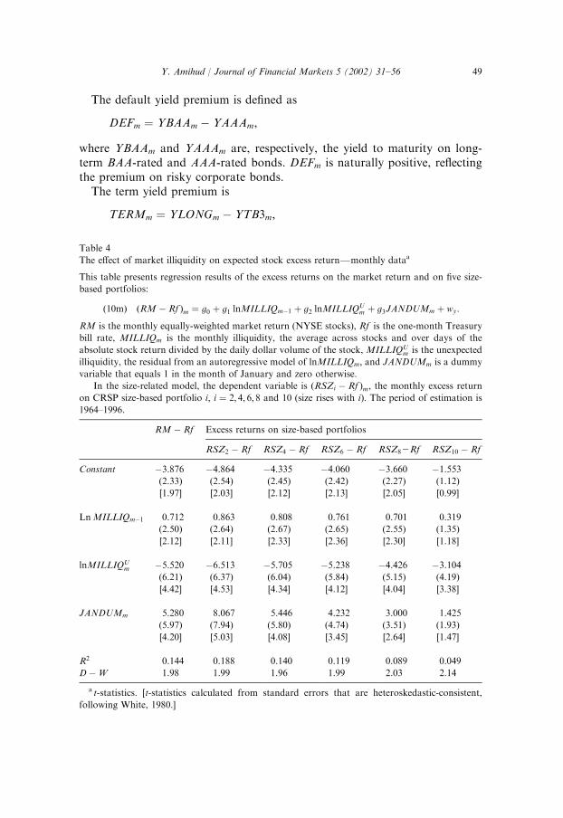
3.3. Monthly data: the effect of illiquidity on stock excess returns

The methodology of the previous two sections is replicated here using monthlydata. There are 408 months in the period 1963–1996. Monthly illiquidity,MILLIQm; is the average across stocks of jRidmj=VOLDidm; the illiquidity measureof stock i on day d in month m; and then averaged over the days of month m: Anautoregressive model similar to (7) is estimated for the monthly data as follows:

lnMILLIQm ¼ 0:313þ 0:945 lnMILLIQm�1 þ residualm

ðt ¼Þ ð3:31Þ ð58:36Þ R2 ¼ 0:89;D�W ¼ 2:34:

ð7mÞ

21The results are qualitatively similar when using the odd-numbered portfolios 1, 3, 5, 7 and 9.


Applying Kendall’s (1954) bias correction method, the adjusted slopecoefficient is 0.954. The estimated parameters are stable over time, as indicatedby the Chow test. Next, the monthly unexpected illiquidity is calculated,MILLIQU

m ; the residual from model (7m) after the coefficients are adjusted.Finally, the monthly version of model (10) is estimated:

ðRM � Rf Þm ¼ g0 þ g1 lnMILLIQm�1 þ g2 lnMILLIQUm

þ g3JANDUMm þ wm:ð10mÞ

This model adds JANDUMm; a January dummy, that accounts for the well-known January effect. RMm is the monthly return on the equally weightedmarket portfolio (for NYSE stocks) and Rf is the one-month Treasury bill rate.The results for the monthly data, presented in Table 4, are qualitatively

similar to those using annual data. In particular, g1 > 0 and g2o0; bothstatistically significant.As a robustness check, the sample of 408 months is divided into six equal

subperiods of 68 months each and model (10m) is estimated for eachsubperiod. The following is a summary of the results:

1. All six coefficients g1 are positive, with mean 0.871 and median 0.827.2. All six coefficients g2 are negative with mean �7.089 and median �5.984.

This shows consistency in the effect of illiquidity.The differences in the effects of illiquidity on different size-based stock

portfolios is tested by estimating model (10m) using excess returns onportfolios corresponding to deciles 2, 4, 6, 8 and 10 (decile 10 contains thelargest firms). The results, presented in Table 4, are again similar to those forthe yearly data: g1 is decreasing in company size, and g2 is increasing incompany size.

3.4. Illiquidity effect, controlling for the effects of bond yield premiums

Two bond yield premiums are known to have a positive effect on exante stock returns over time: the default yield premium (the excess yieldon risky corporate bonds) and the term yield premium (long-term minusshort-term bond yield) (see Keim and Stambaugh, 1986; Fama andFrench, 1989; Fama, 1990).22 The following are tests of the effects of illiquidityon stock excess returns after controlling for the effects of these two yieldpremiums.

22Fama and French (1989) and Fama (1990) study separately the effect of the default premium

and the term premium on ex ante excess stock return. Keim and Stambaugh (1986) combine the

two in a single measure, the difference between the yield on corporate bonds with rating below

BAA and on short-term treasury bills. Boudoukh et al. (1993) study the effect of the term yield on

subsequent stock excess return.


The default yield premium is defined as

DEFm ¼ YBAAm � YAAAm;

where YBAAm and YAAAm are, respectively, the yield to maturity on long-term BAA-rated and AAA-rated bonds. DEFm is naturally positive, reflectingthe premium on risky corporate bonds.The term yield premium is

TERMm ¼ YLONGm � YTB3m;

Table 4

The effect of market illiquidity on expected stock excess returnFmonthly dataa

This table presents regression results of the excess returns on the market return and on five size-

based portfolios:

ð10mÞ ðRM �Rf Þm ¼ g0 þ g1 lnMILLIQm�1 þ g2 lnMILLIQUm þ g3JANDUMm þ wy:

RM is the monthly equally-weighted market return (NYSE stocks), Rf is the one-month Treasury

bill rate, MILLIQm is the monthly illiquidity, the average across stocks and over days of the

absolute stock return divided by the daily dollar volume of the stock,MILLIQUm is the unexpected

illiquidity, the residual from an autoregressive model of lnMILLIQm; and JANDUMm is a dummy

variable that equals 1 in the month of January and zero otherwise.

In the size-related model, the dependent variable is ðRSZi � Rf Þm; the monthly excess returnon CRSP size-based portfolio i; i ¼ 2; 4; 6; 8 and 10 (size rises with i). The period of estimation is1964–1996.

RM �Rf Excess returns on size-based portfolios

RSZ2 � Rf RSZ4 � Rf RSZ6 � Rf RSZ82Rf RSZ10 �Rf

Constant �3.876 �4.864 �4.335 �4.060 �3.660 �1.553(2.33) (2.54) (2.45) (2.42) (2.27) (1.12)

[1.97] [2.03] [2.12] [2.13] [2.05] [0.99]

LnMILLIQm�1 0.712 0.863 0.808 0.761 0.701 0.319

(2.50) (2.64) (2.67) (2.65) (2.55) (1.35)

[2.12] [2.11] [2.33] [2.36] [2.30] [1.18]

lnMILLIQUm �5.520 �6.513 �5.705 �5.238 �4.426 �3.104

(6.21) (6.37) (6.04) (5.84) (5.15) (4.19)

[4.42] [4.53] [4.34] [4.12] [4.04] [3.38]

JANDUMm 5.280 8.067 5.446 4.232 3.000 1.425

(5.97) (7.94) (5.80) (4.74) (3.51) (1.93)

[4.20] [5.03] [4.08] [3.45] [2.64] [1.47]

R2 0.144 0.188 0.140 0.119 0.089 0.049

D�W 1.98 1.99 1.96 1.99 2.03 2.14

a t-statistics. [t-statistics calculated from standard errors that are heteroskedastic-consistent,

following White, 1980.]


where YLONGm and YTB3m are, respectively, the yields on long-term Treasurybonds and three-month Treasury bills. The data source is Basic Economics.The correlations between the variables are low: CorrðlnMILLIQm;DEFmÞ ¼�0:060; CorrðlnMILLIQm;TERMmÞ ¼ 0:021; and CorrðTERMm;DEFmÞ ¼0:068The following model tests the effects of illiquidity on stock excess return,

controlling for the effects of the default and term yield premiums:

ðRM � Rf Þm ¼ g0 þ g1 lnMILLIQm�1 þ g2 lnMILLIQUm þ g3JANDUMm

þ a1DEFm�1 þ a2TERMm�1 þ um: ð11Þ

The model is predictive since lagged illiquidity and bond yields are known toinvestors at the beginning of month m during which ðRM � Rf Þm is observed.The hypothesis that expected illiquidity has a positive effect on ex-ante stockexcess return implies that g1 > 0 and g2o0: In addition, the positive effects ofthe default and term yield premiums imply a1 > 0 and a2 > 0.The results, presented in Table 5, show that lnMILLIQm�1 retains its

positive and significant effect on ex ante stock excess return after controllingfor the default and the term yield premiums. Also, lnAILLIQu

m retains itsnegative effect on contemporaneous stock seen returns. Consistent with Famaand French (1989), the two yield premiums have a positive effect on ex antestock excess return.The differences in the effects of illiquidity on different size-based stock

portfolios is tested again here in the following model, controlling for the effectsof the bond-yield premiums:

ðRSZi � Rf Þm ¼ gi0 þ gi1 lnMILLIQm�1 þ gi2 lnMILLIQUm

þ gi3JANDUMm þ ai1DEFm�1 þ ai2TERMm�1 þ uim; ð11szÞ

where ðRSZi � Rf Þm is the monthly return on CRSP size-portfolio i in excess ofthe one-month T-bill rate, i ¼ 2; 4; 6; 8; 10.The estimation results in Table 5 show the same pattern as before. The

coefficient g1 declines as size increases and the coefficient g2 increases (becomesless negative) as size increases. That is, the illiquidity effect is stronger forsmaller firms.Interestingly, the effect of the default premium varies systematically with

firm size. Since the default premium signifies default risk and future adverseeconomic conditions, it should have a greater effect on the expected return ofsmaller firms that are more vulnerable to adverse conditions. This is indeedthe result: the coefficient of the default premium is declining as the firm sizerises.


Table 5

The effects of expected market illiquidity, default yield premium and term yield premium on

expected stock excess returnFmonthly dataa

Estimation results of the model

ðRM � Rf Þm ¼ g0 þ g1 lnMILLIQm�1 þ g2 lnMILLIQU;m þ g3 JANDUMm ð11Þ

þa1DEFm�1 þ a2TERMm�1 þ um:

ðRM �Rf Þm; the equally-weighted market return in excess of the one month treasury-bill rate formonth m: lnMILLIQm is market illiquidity in month m; calculated as the logarithm of the averageacross stocks over the days of the month of daily absolute stock return divided by the daily dollar

volume of the stock. lnMILLIQUm is the unexpected market illiquidity, the residual from an

autoregressive model of lnMILLIQm: DEFm ¼ YBAAm2YAAAm; where YBAAm and YAAAm are,respectively, the yield to maturity on long term, BAA-rated and AAA-rated corporate bonds.

TERMm ¼ YLONGm2YTB3m; where YLONGm and YTB3m are, respectively, the yields on long-term treasury bonds and three-month Treasury bills. JANDUMm is a dummy variable that equals 1

in the month of January and zero otherwise.

Also estimated is the following model:

ðRSZi � Rf Þm ¼ gi0 þ gi1 lnMILLIQm�1 þ gi2 lnMILLIQUm þ gi3 JANDUMm ð11szÞ

þ ai1DEFm�1 þ ai2TERMm�1 þ uim;

where ðRSZi � Rf Þm is the monthly return on CRSP size-portfolio i in excess of the one-monthT-bill rate, i ¼ 2; 4; 6; 8; 10: The estimation period is 1963–1996.

RM � Rf Excess returns on size-based portfolios

RSZ2 � Rf RSZ4 � Rf RSZ62Rf RSZ8 � Rf RSZ10 � Rf

Constant �5.583 �6.986 �6.170 �6.010 �5.191 �2.693(3.15) (3.43) (3.28) (3.37) (3.03) (1.83)

[2.63] [2.58] [2.73] [2.90] [2.71] [1.68]

LnMILLIQm�1 0.715 0.912 0.846 0.803 0.731 0.332

(2.53) (2.80) (2.82) (2.82) (2.67) (1.41)

[2.18] [2.20] [2.41] [2.48] [2.38] [1.23]

LnMILLIQUm �5.374 �6.281 �5.492 �5.014 �4.242 �2.940

(6.08) (6.18) (5.84) (5.63) (4.95) (3.99)

[4.39] [4.48] [4.27] [4.05] [3.97] [3.26]

JANDUMm 4.981 7.943 5.351 4.128 2.925 1.395

(5.67) (7.86) (5.73) (4.66) (3.44) (1.91)

[4.40] [5.11] [4.11] [3.46] [2.64] [1.48]

DEFm�1 1.193 1.558 1.293 1.386 1.054 0.663

(2.35) (2.66) (2.39) (2.70) (2.14) (1.56)

[2.39] [2.52] [2.30] [2.76] [2.13] [1.54]

TERMm�1 0.281 0.185 0.228 0.227 0.221 0.316

(1.84) (1.05) (1.40) (1.48) (1.50) (2.49)

[1.70] [1.00] [1.31] [1.39] [1.36] [2.30]

R2 0.161 0.205 0.157 0.141 0.106 0.070

D�W 2.00 2.03 1.99 2.03 2.06 2.18

a t-statistics. [t-statistics calculated from standard errors that are heteroskedastic-consistent

following White, 1980.]


4. Summary and conclusion

This paper presents new tests of the proposition that asset expectedreturns are increasing in illiquidity. It is known from earlier studies thatilliquidity explains differences in expected returns across stocks, a resultthat is confirmed here. The new tests in this paper propose that over time,market expected illiquidity affects the ex ante stock excess return. Thisimplies that the stock excess return RM � Rf ; usually referred to as ‘‘riskpremium’’, also provides compensation for the lower liquidity of stocks relativeto that of Treasury securities. And, expected stock excess returns are notconstant but rather vary over time as a function of changes in marketilliquidity.The measure of illiquidity employed in this study is ILLIQ; the ratio

of a stock absolute daily return to its daily dollar volume, averaged oversome period. This measure is interpreted as the daily stock price reaction to adollar of trading volume. While finer and better measures of illiquidity areavailable from market microstructure data on transactions and quotes,23

ILLIQ can be easily obtained from databases that contain daily data on stockreturn and volume. This makes ILLIQ available for most stock markets andenables to construct a time series of illiquidity over a long period of time, whichis necessary for the study of the effects of illiquidity over time.In the cross-section estimations, ILLIQ has a positive effect, consistent with

earlier studies. This is in addition to the usual negative effect of size (stockcapitalization), which is another proxy for liquidity.The new tests of the effects of illiquidity over time show that expected

market illiquidity has a positive and significant effect on ex ante stockexcess return, and unexpected illiquidity has a negative and significant effecton contemporaneous stock return. Market illiquidity is the average ILLIQacross stocks in each period, and expected illiquidity is obtained froman autoregressive model. The negative effect of unexpected illiquidityis because higher realized illiquidity raises expected illiquidity, which inturn leads to higher stock expected return. Then, stock prices should declineto make the expected return rise (assuming that corporate cash flowsare unaffected by market liquidity). The effects of illiquidity on stockexcess return remain significant after including in the model two variablesthat are known to affect expected stock returns: the default yield premium onlow-rated corporate bonds and the term yield premium on long-term Treasurybonds.

23Other measures of illiquidity are the bid–ask spread (Amihud and Mendelson, 1986, the

effective bid–ask spread (Chalmers and Kadlec, 1998), transaction price impact (Brennan and

Subrahmanyam, 1996) or the probability of information-based trading (Easley et al., 1999)Fall

shown to have a positive effect on the cross-section of stock expected return.


The effects over time of illiquidity on stock excess return differ acrossstocks by their liquidity or size: the effects of both expected and unexpectedilliquidity are stronger on the returns of small stock portfolios. Thissuggests that the variations over time in the ‘‘small firm effect’’Ftheexcess return on small firms’ stockFis partially due to changes in marketilliquidity. This is because in times of dire liquidity, there is a ‘‘flight toliquidity’’ that makes large stocks relatively more attractive. The greatersensitivity of small stocks to illiquidity means that these stocks are subject togreater illiquidity risk which, if priced, should result in higher illiquidity riskpremium.The results suggest that the stock excess return, usually referred to as

‘‘risk premium’’, is in part a premium for stock illiquidity. This contributesto the explanation of the puzzle that the equity premium is too high.The results mean that stock excess returns reflect not only the higherrisk but also the lower liquidity of stock compared to Treasurysecurities.

References

Amihud, Y., Mendelson, H., 1980. Dealership market: market making with inventory. Journal of

Financial Economics 8, 311–353.

Amihud, Y., Mendelson, H., 1986. Asset pricing and the bid–ask spread. Journal of Financial

Economics 17, 223–249.

Amihud, Y., Mendelson, H.:; 1989. The effects of beta, bid–ask spread, residual risk and size onstock returns. Journal of Finance 44, 479–486.

Amihud, Y., Mendelson, H., Wood, R., 1990. Liquidity and the 1987 stock market crash. Journal

of Portfolio Management 16, 65–69.

Amihud, Y., Mendelson, H., 1991a. Liquidity, maturity and the yields on U.S. government

securities. Journal of Finance 46, 1411–1426.

Amihud, Y., Mendelson, H., 1991b. Liquidity, asset prices and financial policy. Financial Analysts

Journal 47, 56–66.

Amihud, Y., Mendelson, H., Lauterbach, B., 1997. Market microstructure and

securities values: evidence from the Tel Aviv exchange. Journal of Financial Economics 45,

365–390.

Atkins, A.B., Dyl, E.A., 1997. Transactions costs and holding periods for common stocks. Journal

of Finance 52, 309–325.

Banz, R.W., 1981. The relationship between return and market value of common stocks. Journal of


Barry, C.B., Brown, S.J., 1984. Differential information and the small firm effect. Journal of

Financial Information 13, 283–294.

Berk, J., 1995. A critique of size-related anomalies. Review of Financial Studies 8, 275–286.

Berkman, H., Eleswarapu, V.R., 1998. Short-term traders and liquidity: a test using Bombay stock

exchange data. Journal of Financial Economics 47, 339–355.

Boudoukh, J., Richardson, M., Smith, T., 1993. Is the ex ante risk premium always positive?

Journal of Financial Economics 34, 387–408.


Brennan, M.J., Subrahmanyam, A., 1996. Market microstructure and asset pricing:

on the compensation for illiquidity in stock returns. Journal of Financial Economics 41,

441–464.

Brennan, M.J., Cordia, T., Subrahmanyam, A., 1998. Alternative factor specifications, security

characteristics, and the cross-section of expected stock returns. Journal of Financial Economics

49, 345–373.

Brown, P., Kleidon, A.W., Marsh, T.A., 1983. New evidence on the nature of size-related

anomalies in stock prices. Journal of Financial Econmics 12, 33–56.

Chakravarti, S., Sarkar, A., 1999. Liquidity in U.S. fixed income markets: a comparison of the

bid–ask spread in corporate, government and municipal bond markets. Federal Reserve Bank

of New York, Staff Report Number 73.

Chalmers, J.M.R., Kadlec, G.B., 1998. An empirical examination of the amortized spread. Journal

of Financial Economics 48, 159–188.

Chordia, T., Subrahmanyam, A., Anshuman, V.R., 2001. Trading activity and expected stock

returns. Journal of Financial Economics 59, 3–32.

Constantinides, G.M., Scholes, M.S., 1980. Optimal liquidation of assets in the presence of

personal taxes: implications for asset pricing. Journal of Finance 35, 439–443.

Constantinides, G.M., 1986. Capital market equilibrium with transaction costs. Journal of Political

Economy 94, 842–862.

Coopu, S.K., Goth, J.C., Avera, W.E., 1985. Liquidity, exchange listing and common stock

performance. Journal of Economics and Business 37, 19–33.

Copeland, T.C., Galai, D., 1983. Information effect on the bid–ask spread. Journal of Finance 38,

1457–1469.

Datar, V.T., Naik, N.Y., Radcliffe, R., 1998. Liquidity and stock returns: an alternative test.

Journal of Financial Markets 1, 205–219.

Easley, D., O’Hara, M., 1987. Price, trade size and information in securities markets. Journal of


Easley, D., Hvidkjaer, S., O’Hara, M., 1999. Is information risk a determinant of asset returns?

Working Paper, Cornell University.

Eleswarapu, V.R., Reinganum, M., 1993. The seasonal behavior of liquidity premium in asset

pricing. Journal of Financial Economics 34, 373–386.

Eleswarapu, V.R., 1997. Cost of transacting and expected returns in the NASDAQmarket. Journal

of Finance 52, 2113–2127.

Fama, E.F., MacBeth, J.D., 1973. Risk, return and equilibrium: empirical tests. Journal of Political

Economy 81, 607–636.

Fama, E.F., French, K.R., 1989. Business conditions and expected returns on stocks and bonds.


Fama, E.F., 1990. Stock returns, expected returns, and real activity. Journal of Finance 45,

1089–1108.

Fama, E.F., French, K.R., 1992. The cross section of expected stock returns. Journal of Finance

47, 427–465.

French, K.R., Schwert, G.W., Stambaugh, R.F., 1987. Expected stock returns and volatility.


Glosten, L.R., Milgrom, P.R., 1985. Bid, ask and transaction prices in a specialist market with

heterogeneously informed traders. Journal of Financial Economics 14, 71–100.

Glosten, L., Harris, L., 1988. Estimating the components of the bid–ask spread. Journal of


Harris, M., Raviv, A., 1993. Differences of opinion make a horse race. Review of Financial Studies

6, 473–506.

Harris, L.E., 1994. Minimum price variation, discrete bid–ask spreads, and quotation sizes. Review

of Financial Studies 7, 149–178.


Hasbrouck, J., 1991. Measuring the information content of stock trades. Journal of Finance 46,

179–207.

Haugen, R.A., Baker, N.L., 1996. Commonality in the determinants of expected stock returns.


Hu, S.-Y., 1997a. Trading turnover and expected stock returns: the trading frequency hypothesis

and evidence from the Tokyo Stock Exchange. Working Paper, National Taiwan University.

Kamara, A., 1994. Liquidity, taxes, and short-term treasury yields. Journal of Financial and

Quantitative Analysis 29, 403–416.

Keim, D.B., 1983. Size related anomalies and stock return seasonality. Journal of Financial


Keim, D.B., Stambaugh, R.F., 1986. Predicting returns in the stock and bond market. Journal of


Keim, D.B., Madhavan, A., 1996. The upstairs market for large-block transactions: analysis and

measurement of price effects. Review of Financial Studies 9, 1–36.

Kendall, M.G., 1954. Note on bias in the estimation of autocorrelation. Biometrica 41,

403–404.

Khan, W.A., Baker, H.K., 1993. Unlisted trading privileges, liquidity and stock returns. Journal of

Financial Research 16, 221–236.

Kraus, A., Stoll, H.R., 1972. Price impacts of block trading on the New York Stock Exchange.

Journal of Finance 27, 569–588.

Kyle, A., 1985. Continuous auctions and insider trading. Econometrica 53, 1315–1335.

Levy, H., 1978. Equilibrium in an imperfect market: constraint on the number of securities in the

portfolio. American Economic Review 68, 643–658.

Loughran, T., 1997. Book-to-market across firm size, exchange and seasonality: is there an effect?

Journal of Financial and Quantitative Analysis 32, 249–268.

Merton, R.C., 1987. A simple model of capital market equilibrium with incomplete information.


Newey, W.K., West, K.D., 1987. A simple, positive semi definite, heteroskedasticity and

autocorrelation consistent covariance matrix. Econometrica 55, 703–706.

Pastor, L., Stambaugh, R.F., 2001. Liquidity risk and expected stock returns. Working paper,

Wharton School, University of Pennsylvania, July.

Redding, L.S., 1997. Firm size and dividend payouts. Journal of Financial Intermediation 6,

224–248.

Reinganum, M.R., 1981. Misspecification of capital asset pricing: empirical anomalies based on

earnings yields and market values. Journal of Financial Economics 9, 19–46.

Reinganum, M.R., 1990. Market microstructure and asset pricing. Journal of Financial Economics

28, 127–147.

Rouwenhorst, K.G., 1998. Local return factors and turnover in emerging stock markets. Working

paper, Yale University.

Sawa, T., 1978. The exact moments of the least squares estimator for the autocorregressive model.

Journal of Econometrics 8, 159–172.

Scholes, M., Williams, J., 1977. Estimating betas from non-synchronous data. Journal of Financial


Shumway, T., 1997. The delisting bias in CRSP data. Journal of Finance 52, 327–340.

Silber, W.L., 1975. Thinness in capital markets: the case of the Tel Aviv Stock Exchange. Journal of

Financial and Quantitative Analysis 10, 129–142.

Stambaugh, R.F., 1999. Predictive regressions. Journal of Financial Economics 54,

375–421.

Stigum, M., 1983. The Money Market. Dow Jones-Irwin, Homewood, IL.

Stoll, H.R., 1978. The pricing of security dealers services: an empirical study of NASDAQ stocks.



Stoll, H.R., Whaley, R.H., 1983. Transaction costs and the small firm effect. Journal of Financial


Tinic, S.M., West, R.R., 1986. Risk, return and equilibrium: a revisit. Journal of Political Economy

94, 126–147.


Illiquidityandstockreturns: cross-sectionandtime ...mkearns/finread/amihud.pdf ·...

Documents

Transcript of Illiquidityandstockreturns: cross-sectionandtime ...mkearns/finread/amihud.pdf ·...