Surprise! It’s Illiquid: The January 2006 Tokyo Stock ...mkearns/finread/ronisurpise.pdf · The...

Surprise! It’s Illiquid:

The January 2006 Tokyo Stock Exchange Shutdown

Roni Israelov†

November 29, 2006

Abstract

On January 18, 2006, the Tokyo Stock Exchange (TSE) unexpectedly closed twenty minutesearly. Forty minutes earlier, investors were informed that the number of transactions on thatday had reached the daily capacity of the exchange’s computer systems. Further, the exchangedisclosed that upgrading its technology would take six to twelve months, that the exchangewould shut down automatically on any day in which the daily capacity had been reached, andthat the exchange would close half an hour early each day in the near future to reduce the riskof an unanticipated shutdown. I estimate that over the six month period following the January18 event, the expected number of additional market closures is 1.5 and the probability of atleast one additional shutdown is 70 percent. I investigate the impact of the systematic liquidityevent on relative valuations over the cross-section of stocks listed on the TSE. Stocks that onlytrade on the TSE lost a statistically significant 2 percent of their value relative to those thattrade on the TSE and at least one additional Japanese exchange. Also, liquid stocks lost valuerelative to illiquid stocks. For instance, high turnover stocks lost approximately 6 percent oftheir value relative to low turnover stocks and liquid stocks, as measured by the Amihud (2002)illiquidity measure, lost approximately 4 percent of their value relative to illiquid stocks. Theresults provide further evidence that investors place an economically significant value on liquid-ity.

JEL classification: G0; G1; G12.

Keywords: Liquidity; Market Closure; Liquidity premium; Transaction costs; Tokyo Stock Ex-change.

†Tepper School of Business, Carnegie Mellon University

5000 Forbes Avenue, Pittsburgh, PA 15213, USA

Email: [email protected]

Phone: (412) 606-2796

I am grateful to Burton Hollifield, Lubos Pastor, and Duane Seppi for comments and suggestions.

1 Introduction

On January 18, 2006, the Tokyo Stock Exchange (TSE) unexpectedly closed twenty minutes early.

Forty minutes earlier, investors were informed that the number of transactions on that day, approx-

imately 4.5 million, had reached the exchange’s transaction processing system capacity. Further,

the exchange disclosed that increased capacity through technology upgrades could take six to twelve

months, that the exchange would shut down automatically if and when the daily capacity had been

reached, and that the exchange would close half an hour early each day in the near future to reduce

the risk of another unanticipated shutdown. The event provides a unique opportunity to learn

about the value investors place on liquidity. The market shutdown was not simply a single passing

disruption to the system. The unexpected market closure, coupled with the information disclosed

by the exchange during and after the event, likely led investors to update their beliefs about their

portfolios’ liquidity characteristics. Stocks are not necessarily less liquid – it is possible that the

threshold will not be reached before the systems are sufficiently upgraded. However, the estimated

probability of such an event has increased. Hence, the perceived liquidity risk of holding an asset

listed on the TSE has increased. In addition, the increased probability of an illiquidity event leads

to higher expected future illiquidity for all stocks listed on the exchange. Further, the perceived

change in liquidity is systematic to all TSE traded assets. Where trading volume originates is irrel-

evant; once a certain threshold is met, trading ceases for all assets listed on the exchange. Finally,

changes to liquidity are exogenous in the sense that investors may be fully ready and willing but

simply unable to provide liquidity.

My paper begins with a Monte Carlo analysis designed to estimate the risk of future market closures

due to capacity restrictions. I estimate an AR(1) process for the number of equity transactions

processed at the daily frequency using transactions data for the TSE with sample period October 1,

2005 through the event date and simulate the number of daily transactions over a six month horizon

beginning on the day after the event. I estimate the probability of at least one addition market

closure during the six-month period to be approximately 70 percent and the expected number of

closures during the period to be 1.5. The simulations, which are performed using the information

available on January 18, 2006, indicate that investors on that date had reason to suspect their

1

future ability to trade was lower than previously anticipated.

If the market closure on January 18 led investors to update their beliefs about the liquidity char-

acteristics of their portfolios and if investors require a premium for holding assets with liquidity

risk, then asset prices should change to reflect the new information. I investigate the cross-sectional

variation in changes to asset valuation subsequent to the event. The first component of the analysis

tests for a “flight-to-quality” by comparing the returns of the largest capitalization quintile of stocks

on the TSE to the smallest quintile after controlling for industry effects. Large stocks immediately

experienced a statistically significant 3 percent capital gain relative to small stocks. The shift in

value is persistent and increases to 4 percent over a ten-day period. Because two events, the an-

nounced Livedoor investigation and the market closure, occurred on January 18, it is not clear in

what proportion updated beliefs about liquidity versus fraud contributed to the flight-to-quality.

The second component of my analysis compares the post-event returns of 657 stocks that are traded

only on the TSE to the returns of 297 stocks that are traded on the TSE and at least one other

Japanese exchange. The effect of the TSE market closure on the liquidity of stocks in the latter

group is likely to be smaller because, for these stocks, investors have an additional venue for trade.

I document an immediate and statistically significant 0.5 percent loss in value for the stocks traded

only on the TSE relative to their cross-listed counterparts. The relative capital loss persists and

increases to approximately 2.2 percent over a ten-day period. We may think of cross-listed stocks

as being insured against market closures of any individual exchange and the change in value of the

insurance subsequent to the event equalling approximately 2.2 percent of capitalization. Combining

the estimated change in relative valuations with the Monte Carlo simulations provides an estimated

insurance premium of between 33 and 150 basis points per anticipated market closure.

The final component of my analysis investigates the relative value change for stocks with different

liquidity levels. After sorting stocks on a variety of liquidity-related characteristics, such as turnover,

monetary volume, and the Amihud (2002) illiquidity measure, and controlling for size and industry

effects, I form liquidity portfolios that are long the most liquid assets and short the least liquid

assets. The assets provided to the sorts are those traded only on the TSE to ensure that the change

in ability to trade is approximately homogenous across all stocks. The results of the various liquidity

sorts are mutually consistent; liquid stocks lost value relative to illiquid stocks. For instance, sorting

2

on turnover, the liquidity portfolio has an immediate capital loss of 5 percent that increases to 6

percent over a ten-day period. Sorting on the Amihud (2002) illiquidity measure, the liquidity

portfolio lost approximately 2.5 percent of its value on January 18. The capital loss increased to

almost 4 percent by the end of the month.

My analysis is related to two strings of research on the relationship between returns and the time-

series variation in liquidity. The first set considers value changes due to specific liquidity events.

Amihud, Mendelson, and Lauterbach (1997) investigate the exogenous transfer of stocks listed

on the Tel Aviv Stock Exchange from a once-a-day call auction to semi-continuous trading. They

report that transferred stocks realized a persistent capital gain of 5 to 6 percent. In addition, stocks

that experienced greater improvements in their liquidity had larger capital gains. Muscarella and

Piwowar (2001) consider a similar transfer of stocks from call auctions to a continuous market on the

Paris Bourse and report that the improvements in liquidity were associated with higher valuations.

Hegde and McDermott (2003) investigate the effect of exogenous changes in asset liquidity due to

joining or leaving the S&P 500 Index. They document that liquidity, as measured by Kyle’s λ and

the bid-ask spread, increases upon a stock’s inclusion on the index and that the capital gain that

occurs subsequent to joining the index is positively related to the improved liquidity. The three

papers are methodologically similar because they investigate returns associated with idiosyncratic

liquidity events. My paper is different for two reasons. First, the event I study is a systematic shock

to liquidity. Second, I do not investigate how the valuation of the entire market changed because of

the event. Rather, I study how relative valuations for assets with differing liquidity characteristics

were impacted by the liquidity event.

The second set of literature investigates the relationship between time-series variation in aggregate

liquidity and expected returns. Rather than studying a particular liquidity event, the papers in

this area construct a time series for a measure of aggregate liquidity and consider the covariation

between returns and aggregate liquidity. Amihud (2002) finds that stocks’ excess returns increase

in expected illiquidity and decrease in unexpected illiquidity. He reports that smaller firms have

returns that are more sensitive to changes in aggregate liquidity. Pastor and Stambaugh (2003)

propose and document that stocks’ expected returns increase in their return sensitivities to changes

in market liquidity. Acharya and Pedersen (2005) propose a Liquidity-Adjusted CAPM that relates

3

expected excess returns to expected liquidity levels, systematic gross return risk, and systematic

liquidity risk. One of the three sources of systematic liquidity risk in their model is the asset’s

return sensitivity to changes in aggregate liquidity. They report that less liquid stocks have higher

exposure to liquidity risk. My paper is similar to these papers because I investigate cross-sectional

variation in asset return sensitivities to changes in market liquidity. Unlike the papers in this area,

I do not form an aggregate measure of liquidity and I do not relate the cross-sectional differences

to expected returns. I study the cross-sectional variation in asset return sensitivities to the single

liquidity event on January 18. Interestingly, my findings are not consistent with those reported

by Amihud (2002) and Acharya and Pedersen (2005). Both papers document that illiquid stocks

have returns with greater sensitivities to changes in aggregate liquidity, which is consistent with a

“flight-to-liquidity,” the idea that when liquidity dries up, liquid stocks outperform illiquid stocks.

For the January 18 event studied in this paper, I find that liquid stocks, as inferred by turnover,

monetary volume, and number of transactions or as identified by the Amihud (2002) price-impact

illiquidity measure, experience a statistically significant and persistent capital loss of between 3 to 8

percent relative to illiquid stocks after adjusting for size and industry effects. This finding suggests

that not all negative shocks to aggregate liquidity result in a flight-to-liquidity. Additional research

on how investors re-optimize their portfolios subsequent to liquidity shocks may be warranted to

better understand the circumstances surrounding a flight-to-liquidity, or the lack thereof.

The rest of the paper is organized as follows: The following section presents a brief history of

the event examined in the paper. Section 3 describes the data, the econometric specification, and

reports the results. Section 4 concludes.

2 Background Information

2.1 The Exchanges

Japan has five stock exchanges: Tokyo Stock Exchange (TSE), Osaka Securities Exchange (OSE),

Nagoya Stock Exchange (NSE), Fukuoka Stock Exchange, and Sapporo Securities Exchange. The

first three are the largest in terms of market capitalization and monetary trading volume, and

4

the TSE, the second largest stock exchange in the world by monetary volume, dominates in both

categories. Almost all the research of the Japanese stock market focuses exclusively on the TSE

and the summary statistics described below provide evidence on why this is the case.

Stocks may be traded on more than one exchange. Table 1 presents summary statistics for the

seven permutations of exchange listings using the TSE, OSE, and NSE. The first three rows are

for stocks listed on only one exchange, the next three are for stocks listed on two exchanges, and

the final row is for stocks traded on the three exchanges. The next section provides a complete

description of the data. My sample includes a total of 2847 stocks, 2370 of which are listed on the

TSE. The majority of stocks listed on the TSE are not listed on either of the other two exchanges,

but the majority of stocks listed on the NSE or OSE are also listed on the TSE. For instance,

83 percent of stocks traded on the OSE are also traded on TSE, but only 29 percent of stocks

traded on the TSE are also traded on the OSE. Stocks traded on the TSE have a mean market

capitalization of U216 billion compared to U19 billion for those not traded on the TSE. The market

capitalization of stocks listed on both the TSE and OSE is approximately twice that of those listed

only on the TSE. Stocks listed on all three exchanges are about 12 times larger than those listed

only on the TSE. The 83 percent of stocks traded on the TSE represent 98 percent of the Japanese

stock market capitalization.

Although the OSE and NSE appear to be relatively unimportant when compared against the TSE

and are generally overlooked in the literature, I include the two exchanges in my analysis. Of the

2370 stocks listed on the TSE at 2005 year-end, 1552 stocks are only tradable on the TSE, while

818 stocks are cross-listed on at least one additional Japanese exchange. A TSE market closure

disproportionately affects the liquidity of stocks in the two categories and the first step of my

analysis is to compare the returns of the stocks in the two groups subsequent to the January 18

liquidity event. An alternate approach is to compare stocks traded on the TSE to those that are

not. I do not perform this analysis for two reasons. First, the total market share of stocks not

traded on the TSE is almost insignificant at less than 2 percent. Second, the selection bias, as

evidenced by the differences in mean market capitalization, is likely to be substantial.

5

2.2 The Liquidity Event

In January 2006, the TSE was capable of executing 4.5 million trades per day, approximately 50

percent more than the average number of daily trades in December 2005. Late Monday night on

January 16, prosecutors raided the offices of Livedoor, an upstart Internet portal that had been

popular with small investors. Two days later, the Japanese media reported that Livedoor was

suspected of hiding a U1 billion loss, or $8.7 million, by claiming revenue from three affiliated

companies. Lacking buy orders, Livedoor shares did not trade Wednesday and were marked down

by the daily U100 limit to U496. Many stocks listed on the TSE began to experience a surge

in the number of sell orders. By lunchtime, the president of the TSE announced that the ex-

change processed 2.3 million transactions in morning trading and that trading would likely reach

the exchange’s capacity. At 2:00 pm, an hour before the market’s usual closing time, normally

instantaneous trades were took over 5 minutes to process and the exchange formally announced

that trading would cease 20 minutes early.

After shutting down the exchange early, the TSE announced that the daily trading period will be

shortened by a half-hour until the trading system was upgraded. Investors were given mixed signals;

they were warned that exceeding the 4.5 million trade capacity before the upgrades were complete

would lead to another shutdown and reassured that another shutdown due to excessive volume was

almost impossible. On February 24, 2006 the TSE announced its plans to resume normal trading

hours no later than May. The expected improvements would allow the TSE to process seven million

executions per day.

The event is interesting for a number of reasons. First, the liquidity shock is systematic. Where and

why TSE transactions originate is unimportant. Once a certain threshold is reached, all trading

on the TSE ceases. For the 1552 stocks listed only on the TSE, a market closure represents a

substantial decline in liquidity. Because the remaining 818 stocks listed on the TSE are also listed

on another Japanese exchange, investors’ ability to trade these stocks is less impacted by a TSE

shutdown. Cross-listing acts as an insurance against trading problems that independently affect

a single exchange. Second, a future market shutdown is due to maximum allowable trade and

not restrictions on price movement. The market may close on days with a capital gain as well as

6

those with a capital loss. Finally, the change in liquidity is not due to the traditional sources of

time-varying liquidity. These liquidity risks are not due to spreads or the price impact of trade

increasing because of increased uncertainty or the departure of liquidity traders. Indeed, resolution

of uncertainty that may result in portfolio re-optimization, or an increase in the number of noise

traders, two scenarios generally credited with improvements in market liquidity, may be the cause

of another market closure. In these cases, liquidity traders may be fully ready and willing, but

simply unable to trade.

3 Empirical Analysis

3.1 Data

I analyze stocks listed on the TSE, NSE, and OSE. The list of listed companies for each exchange is

obtained from the exchanges’ respective websites. Transactions data over the period October 1, 2005

through February 28, 2006 is obtained from the TSE for all of its traded stocks. Each observation

includes the price, time, and trade size. The number of shares outstanding is a snapshot taken on

January 31, 2006 from the Marketwatch.com website maintained by Dow Jones. Thus, summary

statistics for market capitalization provided in Table 1 are not adjusted for stock splits or any other

time-variation in the number of outstanding shares. Nikkei 225 Index levels, which I use to proxy

for the Japanese aggregate portfolio, and price and volume information, which I use to calculate

summary statistics in Table 1 for the 477 stocks not traded on the TSE, are also obtained from

Marketwatch.com. Industry classification for each stock listed on the TSE is obtained from the

exchange’s website and is a snapshot taken on November 10, 2006. The industry classification of the

54 stocks that were traded on the TSE at the end of 2005, but were no longer listed on November

10, 2006 is obtained from Bloomberg.com.

3.2 Likelihood of Future TSE Shutdown

The analysis in this paper presupposes that investors revised their expectations of the likelihood

of future market shutdown. Because prices are a forward looking measure of value, if the event is

7

not informative about future ability to trade, there is little reason to suspect that any asymmetric

changes in value follow the event. In this section, I estimate the likelihood of future shutdown.

Figure 1 plots the total number of equity transactions on each day in my sample period. The

spike in transactions that led to the shutdown is visible on January 18, 2006. I calculate the

number of equity transactions on that day to be 2.03 million. However, it is the total number

of transactions cleared by the exchange, including those in the bond and derivative markets, that

is constrained by TSE’s computer systems. Unfortunately, my data does not include non-equity

transactions. To predict the probability that the TSE capacity has been reached, I assume that

the proportion of equity to total transactions is constant over the horizon under investigation.

With the capacity of the exchange on January 18 at approximately 4.5 million, on that day equity

transactions represented approximately 45 percent of total TSE transactions. The Japanese press

reported the average number of transactions in December 2005 to be approximately 3 million per

day. I estimate the average number of equity transactions during the same month to be 1.46 million

per day or approximately 49 percent of the total. The similarity between the two estimates provides

some support for the constant proportion assumption.

I further assume the number of transactions, in millions and denoted by τ , follows an AR(1) process

and estimate the model via OLS with the sample up to and including the event date:

τt+1 = 0.5065 + 0.6363τt + ǫt+1, R2 = 0.3582 σ(ǫ) = 0.1879.

(0.1041) (0.1442)

(1)

Standard errors are in parenthesis. Including a second lag provides a negligible improvement in fit

and the AR(2) coefficient is not statistically significant. Using equation (1), I simulate 25 million

120 day (approximately six months) paths for the number of daily transactions. The shocks used

in the simulations are the residuals from regression (1) resampled with replacement. I include both

signs of each residual to double the error sample size from 70 to 140. I resample the residuals to

avoid making any distributional assumptions on the error process that may remove the ‘outliers’

that are likely responsible for reaching the exchange’s capacity. Predicted market closure occurs

when the simulated number of transactions exceeds 2.03 million, the number of equity transactions

on January 18, 2006.

8

Figure 2 plots the histogram for the simulations. The expected number of shutdowns over the six

month period following the January 18 shutdown is approximately 1.5. The estimated probabilities

of zero and one shutdown, respectively, are 31 and 29 percent. There is a 21 percent chance of three

or more shutdowns, at least one shutdown every two months. The analysis suggests that investors

have reason to believe that future shutdowns are not only possible, but also probable. Hence, any

negative value associated with the new information about future potential liquidity events may be

reflected in price movements subsequent to the January 18 market closure.

3.3 Relative Value Changes

This section investigates the effect of the January 18 shutdown on relative valuations. The general

strategy for the analysis is summarized by the following outline:

1. For each asset, I estimate the cumulative simple return obtained by purchasing the stock on

January 17, 2006 and selling the stock on each of the remaining 10 trading days in January.

2. Assets are sorted on liquidity-related characteristics, such as turnover and Amihud (2002)’s

illiquidity measure.

3. Zero-cost portfolios are formed that are long and short, respectively, the liquid and illiquid

quintile from the previous step sort.

4. I estimate the relative value change of the liquidity portfolios over the 10 day period.

For the first step, I estimate the cumulative simple return with and without adjusting for a market

factor, which I represent by the Nikkei 225 Index. The former approach is denoted by “market-

adjusted cumulative returns” and the latter by “unadjusted.” There is evidence that factor models

may not be successful in explaining Japanese stock returns. Research by Hawawini (1991) indicates

that the market factor cannot explain Japanese cross-sectional stock returns. Daniel, Titman, and

Wei (2001) show that Japanese stock returns are more closely related to their book-to-market ratios

than United States stocks and reject the Fama and French (1993) three-factor model. Hu (1997),

who investigates the impact of liquidity as measured by asset turnover on asset pricing on the TSE,

does not include the market factor in regressions. I include the market-adjusted cumulative returns

9

for robustness.

The cumulative simple return for each stock is estimated via the following OLS regression,

rit = αi + βirmt I +

10∑

d=1

αidψd,t + ǫit, (2)

where rit is the daily log return for asset i at time t, rmt is the log return for the Nikkei 225 Index,

I is 1 for the market-adjusted model and 0 otherwise, and ψd,t is 1 on the dth trading day after

January 17, 2006 and 0 otherwise. The cumulative simple return is then

Rid ≡ exp

(

10∑

d=1

αid

)

− 1. (3)

Further detail on the second and third steps are provided in the relevant sections. The output of the

two steps are a set of NL and NS assets, respectively, that are the long and short components of the

portfolio of interest and their market-adjusted and unadjusted cumulative returns. The cumulative

return for the portfolio is then calculated to be

Rpd =

1

NL

NL∑

i=1

Rid,L −1

NS

NS∑

i=1

Rid,S , (4)

where Rid,L is the return of asset i within the long component of the portfolio and Rid,S is similarly

defined for the short component. I provide two metrics for testing the statistical significance of the

portfolio’s cumulative returns. The first metric is the standard error of the portfolio’s cumulative

return on each day and is used to test whether the relative change in value of the portfolio is

significantly different than zero. The standard error is calculated to be

se(

Rpd

)

=

[

N− 3

2L

NL∑

i=1

(

Rid,L − Rd,L)2

+N− 3

2S

NS∑

i=1

(

Rid,S − Rd,S)2

]

12

, (5)

where Rd,L and Rd,S are the equal-weight cumulative returns, respectively, for the NL and NS

assets that are purchased and sold. The second metric is the standard error of a randomly formed

portfolio with the same structure, long and short NL and NS randomly selected stocks. The metric

allows for testing whether the liquidity portfolio’s return is statistically different than a similarly

10

structured randomly-formed portfolio. The standard error is calculated to be

se(

Rrandd

)

=

√

NL +NS

NLNS

· se(

Rpopd

)

, (6)

where se(

Rpopd

)

is the standard error of the d-day cumulative return for the population being

sampled from when forming the benchmark portfolio. The derivation of equation (6) is included in

the Appendix.

3.3.1 Industry Effects

The market closure was not the only event on January 18 that may have led to asymmetric changes

in valuation. Indeed, the closure occurred because of a surge in transactions due to new information

about alleged fraudulent activity by one of Japan’s most popular internet companies. It is likely

that the cause of the spike in trading activity may itself lead to shifts in market valuations across

industries.

In addition to exchange-traded funds and real estate investment trusts, TSE categorizes stocks

according to 33 industry classifications. Table 2 details the number of stocks within each industry

classification for the 1552 stocks that are only traded on the TSE. I aggregate industry classifications

into 11 groups. For instance, the first group contains the five industries related to transportation

and the second group includes the five finance related industries. As will soon be clarified, I sort

stocks according to certain asset characteristics within each industry group. The reason for the

aggregation is to ensure that each group contains a sufficient number of stocks which is not the

case for individual industries.

Table 3 reports the cumulative returns estimated using the unadjusted model for the 11 in-

dustry groups. Every industry group experienced a capital loss on January 18. The informa-

tion/communication group, which is the group that contains Livedoor, had the largest capital loss,

7.9 percent, followed by services with a 7.8 percent loss. By the end of the month, as revealed by

R10, every group except for wholesale/retail, services, and information/communication had fully

recovered the initial capital loss that occurred on January 18. For instance, the machinery group

went from an initial capital loss of 6.5 percent to a 3.25 percent capital gain.

11

These results suggest that over the period of interest there were industry effects that may influence

the analysis. If, for example, stocks within the information/communication group have different

liquidity characteristics than those within construction, then sorting on liquidity-related attributes

and examining the return of the liquidity portfolio may falsely attribute shifts in industry valuation

to those related to liquidity.

For the remainder of the paper, when I form zero-cost portfolios, I control for industry in the

following manner. I sort assets within each industry group on the characteristic of interest. A

portfolio is then formed by buying and selling an approximately equal number of stocks from

each industry group. For instance, if portfolios are formed subsequent to a quintile ranking, then

approximately 30 stocks within the services group will be in the long and short portfolios. The total

proportion of stocks from each group in the final industry-neutral portfolio is approximately equal

to its proportion in the aggregate portfolio, so the representation of each industry is unaffected

by the control. Because for each industry, the long and short positions contain approximately the

same number of stocks, industry effects are neutralized by the offsetting positions.

3.3.2 Size Effects

Both events on January 18, the announced Livedoor investigation and the market closure, may

independently lead to a flight-to-quality. If investors are concerned that the fraudulent activity

may extend beyond Livedoor, they may be tempted to shift their portfolios to higher quality firms.

Similarly, if investors believe that they may have difficulty trading in the future, they may prefer

their portfolios to be weighted towards more stable firms. Assuming that quality and size are

positively related, the flight-to-quality may be tested by looking for a size effect. I form industry-

adjusted quintile-ranked portfolios after sorting stocks listed only on the TSE by their respective

time-series average daily market capitalization over the period October 1, 2005 to December 31,

2005. The final portfolio is long the 309 firms with the highest market capitalization and short the

307 stocks with the lowest market capitalization.

Table 4 reports the cumulative returns for the market adjusted and unadjusted models and Figure

4 plots the returns. There is an immediate and persistent shift in relative value towards larger

12

firms. In the market adjusted model, large-cap stocks have an initial 4 percent capital gain relative

to small-cap stocks. The initial capital gain drops to 3 percent over the ten day holding period.

The unadjusted results are similar with an initial relative capital gain of 3 percent that grows to 4

percent over the ten-day period.

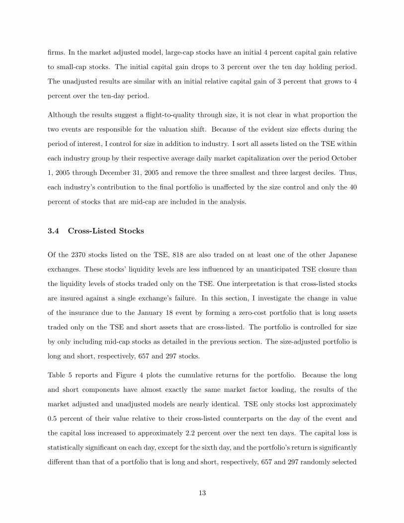
Although the results suggest a flight-to-quality through size, it is not clear in what proportion the

two events are responsible for the valuation shift. Because of the evident size effects during the

period of interest, I control for size in addition to industry. I sort all assets listed on the TSE within

each industry group by their respective average daily market capitalization over the period October

1, 2005 through December 31, 2005 and remove the three smallest and three largest deciles. Thus,

each industry’s contribution to the final portfolio is unaffected by the size control and only the 40

percent of stocks that are mid-cap are included in the analysis.

3.4 Cross-Listed Stocks

Of the 2370 stocks listed on the TSE, 818 are also traded on at least one of the other Japanese

exchanges. These stocks’ liquidity levels are less influenced by an unanticipated TSE closure than

the liquidity levels of stocks traded only on the TSE. One interpretation is that cross-listed stocks

are insured against a single exchange’s failure. In this section, I investigate the change in value

of the insurance due to the January 18 event by forming a zero-cost portfolio that is long assets

traded only on the TSE and short assets that are cross-listed. The portfolio is controlled for size

by only including mid-cap stocks as detailed in the previous section. The size-adjusted portfolio is

long and short, respectively, 657 and 297 stocks.

Table 5 reports and Figure 4 plots the cumulative returns for the portfolio. Because the long

and short components have almost exactly the same market factor loading, the results of the

market adjusted and unadjusted models are nearly identical. TSE only stocks lost approximately

0.5 percent of their value relative to their cross-listed counterparts on the day of the event and

the capital loss increased to approximately 2.2 percent over the next ten days. The capital loss is

statistically significant on each day, except for the sixth day, and the portfolio’s return is significantly

different than that of a portfolio that is long and short, respectively, 657 and 297 randomly selected

13

TSE listed stocks. If the simulated number of shutdowns in Section 3.2 is consistent with investors’

beliefs, then we may extrapolate that insurance against TSE shutdown is valued at approximately

33 to 150 basis points per anticipated closure.

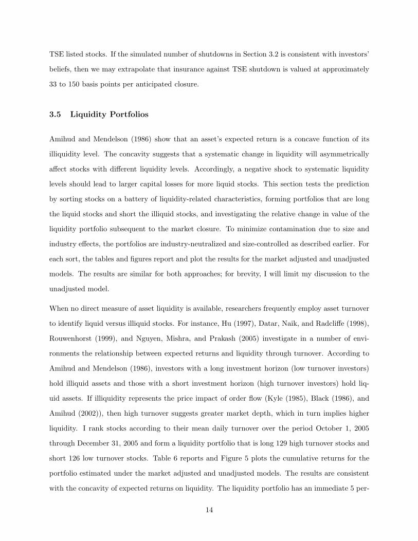
3.5 Liquidity Portfolios

Amihud and Mendelson (1986) show that an asset’s expected return is a concave function of its

illiquidity level. The concavity suggests that a systematic change in liquidity will asymmetrically

affect stocks with different liquidity levels. Accordingly, a negative shock to systematic liquidity

levels should lead to larger capital losses for more liquid stocks. This section tests the prediction

by sorting stocks on a battery of liquidity-related characteristics, forming portfolios that are long

the liquid stocks and short the illiquid stocks, and investigating the relative change in value of the

liquidity portfolio subsequent to the market closure. To minimize contamination due to size and

industry effects, the portfolios are industry-neutralized and size-controlled as described earlier. For

each sort, the tables and figures report and plot the results for the market adjusted and unadjusted

models. The results are similar for both approaches; for brevity, I will limit my discussion to the

unadjusted model.

When no direct measure of asset liquidity is available, researchers frequently employ asset turnover

to identify liquid versus illiquid stocks. For instance, Hu (1997), Datar, Naik, and Radcliffe (1998),

Rouwenhorst (1999), and Nguyen, Mishra, and Prakash (2005) investigate in a number of envi-

ronments the relationship between expected returns and liquidity through turnover. According to

Amihud and Mendelson (1986), investors with a long investment horizon (low turnover investors)

hold illiquid assets and those with a short investment horizon (high turnover investors) hold liq-

uid assets. If illiquidity represents the price impact of order flow (Kyle (1985), Black (1986), and

Amihud (2002)), then high turnover suggests greater market depth, which in turn implies higher

liquidity. I rank stocks according to their mean daily turnover over the period October 1, 2005

through December 31, 2005 and form a liquidity portfolio that is long 129 high turnover stocks and

short 126 low turnover stocks. Table 6 reports and Figure 5 plots the cumulative returns for the

portfolio estimated under the market adjusted and unadjusted models. The results are consistent

with the concavity of expected returns on liquidity. The liquidity portfolio has an immediate 5 per-

14

cent capital loss on the day of the market closure. The capital loss is persistent and increases by an

additional one percent over the ten-day period. The result is statistically significant over the entire

period and the portfolio’s return difference from that of a similarly structured randomly-formed

portfolio is also statistically significant.

For robustness, I consider several additional measures of market depth. Table 8 and Figure 7

provides the cumulative returns for assets sorted by their average number of daily transactions.

Table 10 and Figure 9 report the returns for assets sorted by their average daily monetary volume1,

which is defined as the sum of the price times volume over each transaction during the day. Table

7 and Figure 6 give the relative value change for the liquidity portfolio formed by sorting stocks on

their average turnover per trade, which is defined as the daily turnover divided by the number of

transactions. Sorting by the number of daily transactions, the liquidity portfolio has an initial 3.7

percent capital loss that increases to 5.2 percent by the end of the month. For the liquidity portfolio

formed after sorting by monetary volume, the initial relative loss in value is 4.1 percent. The loss

increases to 6 percent over the ten-day period. Approximately 2.8 percent in value is immediately

lost for the portfolio formed after sorting by asset turnover per transaction. The capital loss

increases to 3.8 percent by the end of the period. The returns are statistically significant and

statistically different than those of a similarly structured portfolio with assets selected randomly.

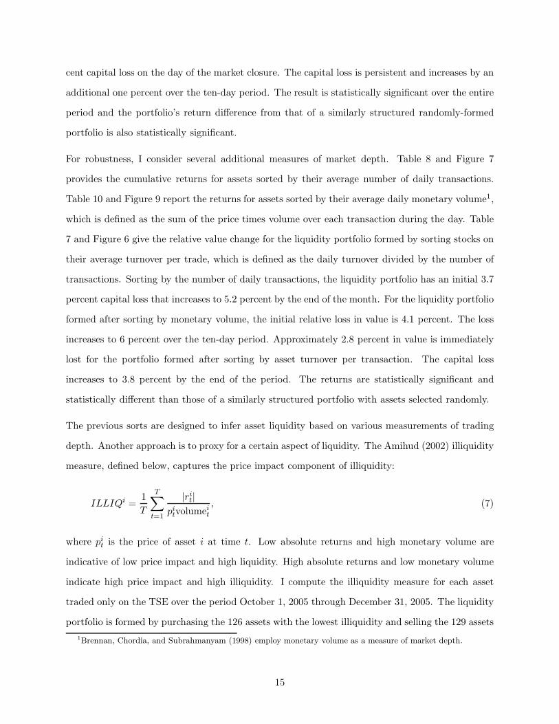
The previous sorts are designed to infer asset liquidity based on various measurements of trading

depth. Another approach is to proxy for a certain aspect of liquidity. The Amihud (2002) illiquidity

measure, defined below, captures the price impact component of illiquidity:

ILLIQi =1

T

T∑

t=1

|rit|

pitvolumeit, (7)

where pit is the price of asset i at time t. Low absolute returns and high monetary volume are

indicative of low price impact and high liquidity. High absolute returns and low monetary volume

indicate high price impact and high illiquidity. I compute the illiquidity measure for each asset

traded only on the TSE over the period October 1, 2005 through December 31, 2005. The liquidity

portfolio is formed by purchasing the 126 assets with the lowest illiquidity and selling the 129 assets

1Brennan, Chordia, and Subrahmanyam (1998) employ monetary volume as a measure of market depth.

15

with the highest illiquidity. The portfolio is industry-neutralized and size-controlled. Table 9 and

Figure 8 provide the results for the liquidity portfolio through the Amihud illiquidity sort. The

performance of the liquidity portfolio over the ten day period is consistent with the concavity effect.

Liquid stocks experience an initial and persistent 2.5 percent capital loss. The capital loss increases

to almost 4 percent over the ten day period. The relative loss in value of the liquidity portfolio is

statistically significant and the performance of the portfolio is statistically different than that of a

randomly-formed portfolio.

It is interesting to investigate whether there is any correspondence between the assets inferred to

be illiquid from the turnover sort and those that are estimated to be illiquid based on the Amihud

(2002) illiquidity measure. I form a portfolio that is long assets identified to be liquid by the turnover

criteria and the Amihud illiquidity measure and short assets identified to be illiquid through the two

sorts. Because the portfolios are quintile ranked, if the two measures are independent, the long and

short portfolios should each have approximately 0.20∗126 = 25 stocks. The double sorted portfolio

is long and short, respectively, 80 and 82 stocks. Approximately 64 percent of stocks identified as

liquid by the turnover sort are also categorized as liquid by the illiquidity measure, suggesting that

the two criteria capture a common component of liquidity. The proportion is similar for the illiquid

stocks. Table 12 and Figure 11 present the results for the liquidity portfolio. The cumulative

returns for the double sort are nearly identical to those obtained by the original turnover sorted

portfolios.

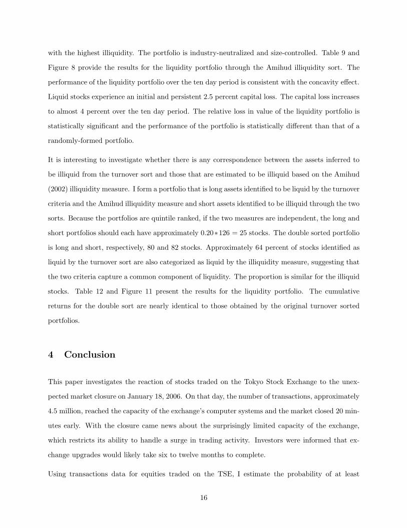
4 Conclusion

This paper investigates the reaction of stocks traded on the Tokyo Stock Exchange to the unex-

pected market closure on January 18, 2006. On that day, the number of transactions, approximately

4.5 million, reached the capacity of the exchange’s computer systems and the market closed 20 min-

utes early. With the closure came news about the surprisingly limited capacity of the exchange,

which restricts its ability to handle a surge in trading activity. Investors were informed that ex-

change upgrades would likely take six to twelve months to complete.

Using transactions data for equities traded on the TSE, I estimate the probability of at least

16

one market closure over the subsequent six-month period to be approximately 70 percent and the

expected number of closures to be approximately 1.5. Hence, investors have reason to suspect that

they may have difficulty trading in the near future. I compare the relative change in value of the

657 stocks that are only traded on the TSE to that of the 297 stocks that are also listed on either

the Osaka Securities Exchange, or the Nagoya Stock Exchange, or both. I report that the stocks

only traded on the TSE experienced an approximate 2.2 percent capital loss relative to the stocks

with an additional avenue for trade in the case of another TSE closure. I also compare the change

in value of liquid stocks to illiquid stocks by sorting on a number of liquidity-related characteristics,

such as asset turnover and the Amihud (2002) illiquidity measure. The results of the analysis are

consistent with the concavity of expected returns in liquidity detailed by Amihud and Mendelson

(1986). Each sort and portfolio formation confirms that liquid stocks lost value relative to illiquid

stocks. For instance, over the ten-day period subsequent to the market closure, high turnover

stocks experienced a statistically significant 6.2 percent capital loss relative to low turnover stocks.

These shifts in value are inconsistent with the findings of Amihud (2002) and Acharya and Pedersen

(2005), who document that illiquid stocks have returns with greater sensitivity to changes in market

liquidity. Their findings support the notion of flight-to-liquidity, which suggests that liquid stocks

outperform illiquid stocks in times of reduced liquidity. The natural question following the apparent

inconsistency between their results and those reported in this paper is: why does a positive shock

to aggregate liquidity, as measured by the Amihud (2002) illiquidity measure, lead to a flight-to-

liquidity, while the increased illiquidity due to the risk of unanticipated market closure in Japan

result in a flight-from-liquidity? Additional research on the economics behind return sensitivities

to changes in systematic liquidity may provide the answer.

The relatively large value shifts after the January 18 market closure are surprising. The market

is not guaranteed to fail again. Even if the TSE reaches capacity and shuts down before its

computer systems are sufficiently upgraded, an unanticipated market closure is likely to result in

only a temporary loss in liquidity that automatically ‘resets’ the next day. It is not clear whether

investors overreacted to the news or rationally updated their beliefs about the exchange’s ability to

consistently provide liquidity. Perhaps the exchange’s failure to provide adequate trading capacity is

indicative of additional undiscovered problems. Regardless, the unexpected market closure coupled

17

with the asymmetric changes in asset valuations provides additional evidence that investors place

an economically significant value on the liquidity of their holdings.

18

References

Acharya, V. V., and L. H. Pedersen (2005): “Asset Pricing with Liquidity Risk,” Journal of

Financial Economics, 77, 375–410.

Amihud, Y. (2002): “Illiquidity and Stock Returns: Cross-Section and Time-Series Effects,” Jour-

nal of Financial Markets, 5, 31–56.

Amihud, Y., and H. Mendelson (1986): “Asset pricing and the Bid-Ask Spread,” Journal of


Amihud, Y., H. Mendelson, and B. Lauterbach (1997): “Market Microstructure and Securi-

ties Values: Evidence from the Tel Aviv Stock Exchange,” Journal of Financial Economics, 45,

365–390.

Black, F. (1986): “Noise,” Journal of Finance, 41, 529–543.

Brennan, M. J., T. Chordia, and A. Subrahmanyam (1998): “Alternative Factor Specifica-

tions, Security Characteristics, and hte Cross-Section of Expected Stock Returns,” Journal of


Daniel, K., S. Titman, and J. Wei (2001): “Explaining the Cross-Section of Stock Returns in

Japan: Factors or Characteristics?,” Journal of Finance, 56, 743–766.

Datar, V. T., N. Y. Naik, and R. Radcliffe (1998): “Liquidity and Stock Returns: An

Alternative Test – Market-Making with Inventory,” Journal of Financial Markets, 1, 205–219.

Fama, E. F., and K. R. French (1993): “Common Risk Factors in the Returns on Stocks and

Bonds,” Journal of Finance, 33, 5–56.

Hawawini, G. A. (1991): Stock Market Anomolies and the Pricing of Equities on the Tokyo Stock

Exchange. Elsevier Science Publishers B.V.

Hegde, S. P., and J. B. McDermott (2003): “The Liquidity Effects of Revisions to the S&P

500 Index: An Empirical Analysis,” Journal of Financial Markets, 6, 413–459.

Hu, S.-Y. (1997): “Trading Turnover and Expected Stock Returns: The Trading Frequency Hy-

19

pothesis and Evidence from the Tokyo Stock Exchange,” Working Paper, National Taiwan Uni-

versity and University of Chicago.

Kyle, A. S. (1985): “Continuous Auctions and Insider Trading,” Econometrica, 53, 1315–1335.

Muscarella, C. J., and M. S. Piwowar (2001): “Market Microstructure and Securities Values:

Evidence from the Paris Bourse,” Journal of Financial Markets, 4, 209–229.

Nguyen, D., S. Mishra, and A. J. Prakash (2005): “On Compensation for Illiquidity in

Asset Pricing: An Empirical Evaluation using Three-Factor Model and Three-Moment CAPM,”

(Working Paper) Florida International University, Miami Florida.

Pastor, L., and R. F. Stambaugh (2003): “Liquidity Risk and Expected Stock Returns,”

Journal of Political Economy, 111, 642–685.

Rouwenhorst, K. G. (1999): “Local Return Factors and Turnover in Emerging Stock Markets,”

Journal of Finance, 54, 1439–1464.

20

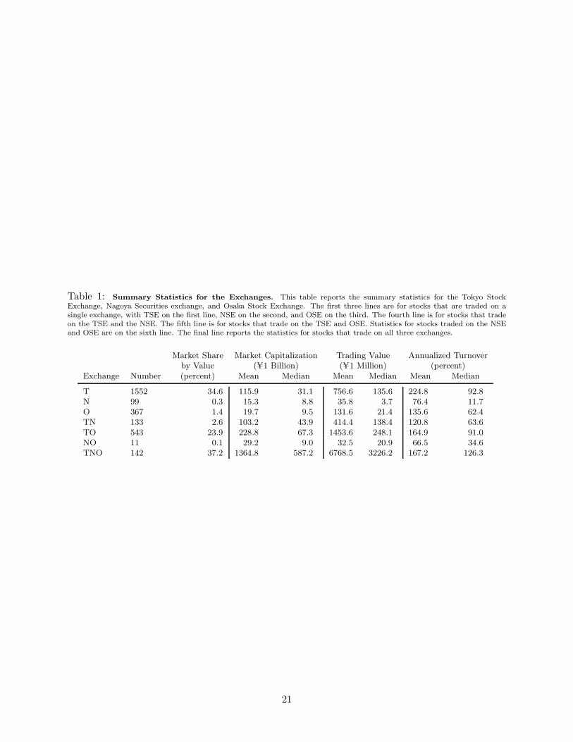
Table 1: Summary Statistics for the Exchanges. This table reports the summary statistics for the Tokyo StockExchange, Nagoya Securities exchange, and Osaka Stock Exchange. The first three lines are for stocks that are traded on asingle exchange, with TSE on the first line, NSE on the second, and OSE on the third. The fourth line is for stocks that tradeon the TSE and the NSE. The fifth line is for stocks that trade on the TSE and OSE. Statistics for stocks traded on the NSEand OSE are on the sixth line. The final line reports the statistics for stocks that trade on all three exchanges.

Market Share Market Capitalization Trading Value Annualized Turnoverby Value (U1 Billion) (U1 Million) (percent)

Exchange Number (percent) Mean Median Mean Median Mean Median

T 1552 34.6 115.9 31.1 756.6 135.6 224.8 92.8N 99 0.3 15.3 8.8 35.8 3.7 76.4 11.7O 367 1.4 19.7 9.5 131.6 21.4 135.6 62.4TN 133 2.6 103.2 43.9 414.4 138.4 120.8 63.6TO 543 23.9 228.8 67.3 1453.6 248.1 164.9 91.0NO 11 0.1 29.2 9.0 32.5 20.9 66.5 34.6TNO 142 37.2 1364.8 587.2 6768.5 3226.2 167.2 126.3

21

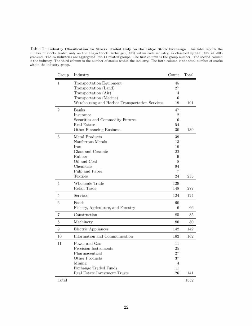
Table 2: Industry Classification for Stocks Traded Only on the Tokyo Stock Exchange. This table reports thenumber of stocks traded only on the Tokyo Stock Exchange (TSE) within each industry, as classified by the TSE, at 2005year-end. The 35 industries are aggregated into 11 related groups. The first column is the group number. The second columnis the industry. The third column is the number of stocks within the industry. The forth column is the total number of stockswithin the industry group.

Group Industry Count Total

1 Transportation Equipment 45Transportation (Land) 27Transportation (Air) 4Transportation (Marine) 6Warehousing and Harbor Transportation Services 19 101

2 Banks 47Insurance 2Securities and Commodity Futures 6Real Estate 54Other Financing Business 30 139

3 Metal Products 39Nonferrous Metals 13Iron 19Glass and Ceramic 22Rubber 9Oil and Coal 8Chemicals 94Pulp and Paper 7Textiles 24 235

4 Wholesale Trade 129Retail Trade 148 277

5 Services 124 124

6 Foods 60Fishery, Agriculture, and Forestry 6 66

7 Construction 85 85

8 Machinery 80 80

9 Electric Appliances 142 142

10 Information and Communication 162 162

11 Power and Gas 11Precision Instruments 25Pharmaceutical 27Other Products 37Mining 4Exchange Traded Funds 11Real Estate Investment Trusts 26 141

Total 1552

22

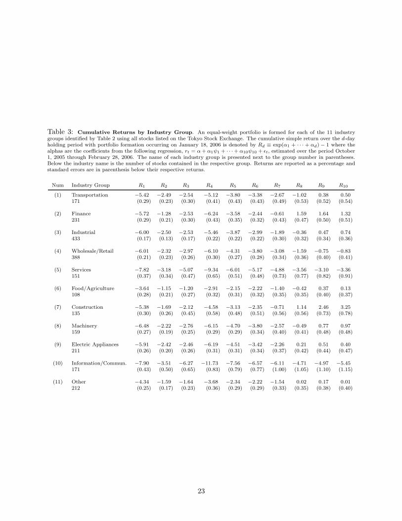
Table 3: Cumulative Returns by Industry Group. An equal-weight portfolio is formed for each of the 11 industrygroups identified by Table 2 using all stocks listed on the Tokyo Stock Exchange. The cumulative simple return over the d-dayholding period with portfolio formation occurring on January 18, 2006 is denoted by Rd ≡ exp(α1 + · · · + αd) − 1 where thealphas are the coefficients from the following regression, rt = α+ α1ψ1 + · · ·+ α10ψ10 + ǫt, estimated over the period October1, 2005 through February 28, 2006. The name of each industry group is presented next to the group number in parentheses.Below the industry name is the number of stocks contained in the respective group. Returns are reported as a percentage andstandard errors are in parenthesis below their respective returns.

Num Industry Group R1 R2 R3 R4 R5 R6 R7 R8 R9 R10

(1) Transportation −5.42 −2.49 −2.54 −5.12 −3.80 −3.38 −2.67 −1.02 0.38 0.50171 (0.29) (0.23) (0.30) (0.41) (0.43) (0.43) (0.49) (0.53) (0.52) (0.54)

(2) Finance −5.72 −1.28 −2.53 −6.24 −3.58 −2.44 −0.61 1.59 1.64 1.32231 (0.29) (0.21) (0.30) (0.43) (0.35) (0.32) (0.43) (0.47) (0.50) (0.51)

(3) Industrial −6.00 −2.50 −2.53 −5.46 −3.87 −2.99 −1.89 −0.36 0.47 0.74433 (0.17) (0.13) (0.17) (0.22) (0.22) (0.22) (0.30) (0.32) (0.34) (0.36)

(4) Wholesale/Retail −6.01 −2.32 −2.97 −6.10 −4.31 −3.80 −3.08 −1.59 −0.75 −0.83388 (0.21) (0.23) (0.26) (0.30) (0.27) (0.28) (0.34) (0.36) (0.40) (0.41)

(5) Services −7.82 −3.18 −5.07 −9.34 −6.01 −5.17 −4.88 −3.56 −3.10 −3.36151 (0.37) (0.34) (0.47) (0.65) (0.51) (0.48) (0.73) (0.77) (0.82) (0.91)

(6) Food/Agriculture −3.64 −1.15 −1.20 −2.91 −2.15 −2.22 −1.40 −0.42 0.37 0.13108 (0.28) (0.21) (0.27) (0.32) (0.31) (0.32) (0.35) (0.35) (0.40) (0.37)

(7) Construction −5.38 −1.69 −2.12 −4.58 −3.13 −2.35 −0.71 1.14 2.46 3.25135 (0.30) (0.26) (0.45) (0.58) (0.48) (0.51) (0.56) (0.56) (0.73) (0.78)

(8) Machinery −6.48 −2.22 −2.76 −6.15 −4.70 −3.80 −2.57 −0.49 0.77 0.97159 (0.27) (0.19) (0.25) (0.29) (0.29) (0.34) (0.40) (0.41) (0.48) (0.48)

(9) Electric Appliances −5.91 −2.42 −2.46 −6.19 −4.51 −3.42 −2.26 0.21 0.51 0.40211 (0.26) (0.20) (0.26) (0.31) (0.31) (0.34) (0.37) (0.42) (0.44) (0.47)

(10) Information/Commun. −7.90 −3.51 −6.27 −11.73 −7.56 −6.57 −6.11 −4.71 −4.97 −5.45171 (0.43) (0.50) (0.65) (0.83) (0.79) (0.77) (1.00) (1.05) (1.10) (1.15)

(11) Other −4.34 −1.59 −1.64 −3.68 −2.34 −2.22 −1.54 0.02 0.17 0.01212 (0.25) (0.17) (0.23) (0.36) (0.29) (0.29) (0.33) (0.35) (0.38) (0.40)

23

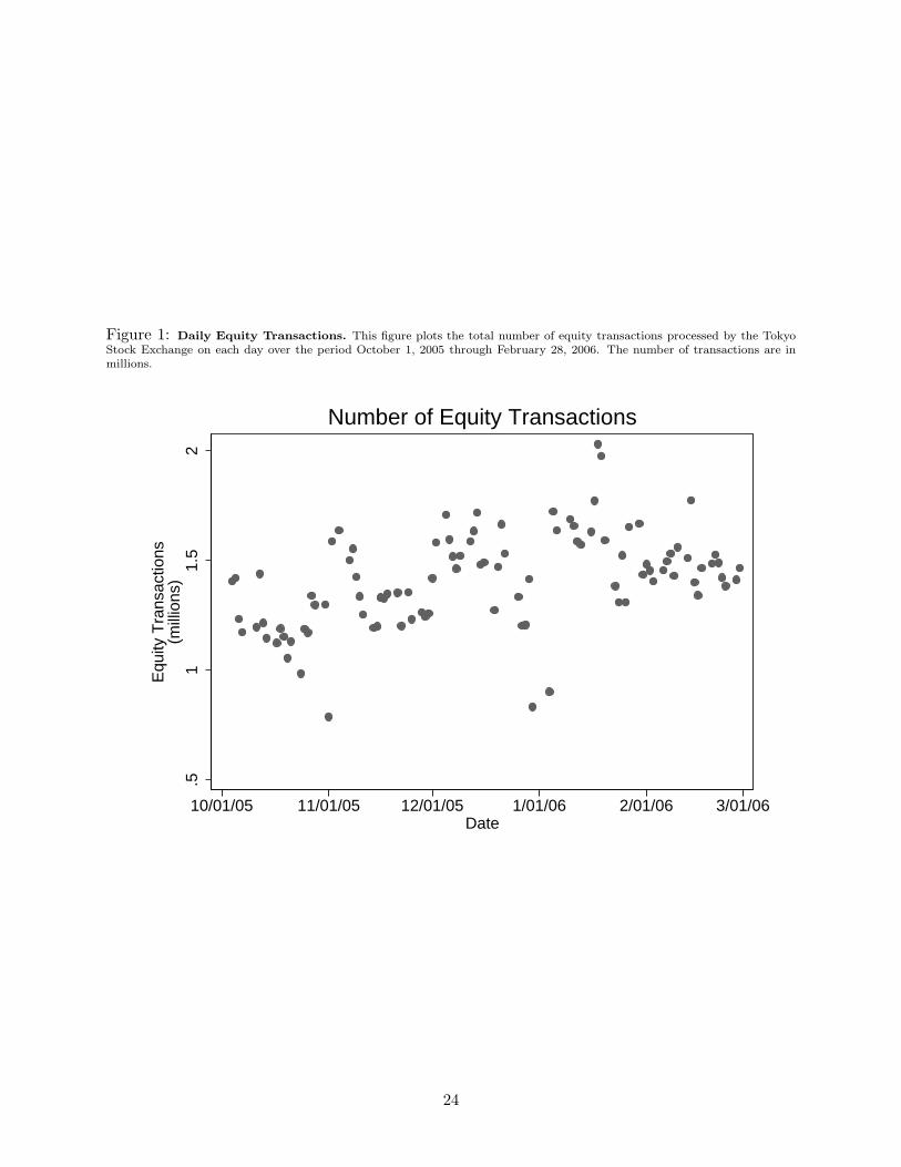
Figure 1: Daily Equity Transactions. This figure plots the total number of equity transactions processed by the TokyoStock Exchange on each day over the period October 1, 2005 through February 28, 2006. The number of transactions are inmillions.

.51

1.5

2

Equ

ity T

rans

actio

ns(m

illio

ns)

10/01/05 11/01/05 12/01/05 1/01/06 2/01/06 3/01/06Date

Number of Equity Transactions

24

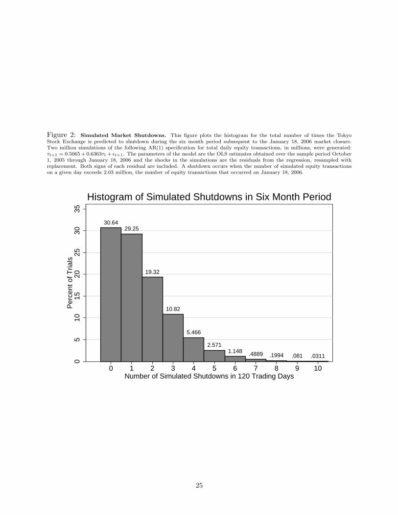
Figure 2: Simulated Market Shutdowns. This figure plots the histogram for the total number of times the TokyoStock Exchange is predicted to shutdown during the six month period subsequent to the January 18, 2006 market closure.Two million simulations of the following AR(1) specification for total daily equity transactions, in millions, were generated:τt+1 = 0.5065 + 0.6363τt + ǫt+1. The parameters of the model are the OLS estimates obtained over the sample period October1, 2005 through January 18, 2006 and the shocks in the simulations are the residuals from the regression, resampled withreplacement. Both signs of each residual are included. A shutdown occurs when the number of simulated equity transactionson a given day exceeds 2.03 million, the number of equity transactions that occurred on January 18, 2006.

30.6429.25

19.32

10.82

5.466

2.5711.148 .4889 .1994 .081 .0311

05

1015

2025

3035

Per

cent

of T

rials

0 1 2 3 4 5 6 7 8 9 10Number of Simulated Shutdowns in 120 Trading Days

Histogram of Simulated Shutdowns in Six Month Period

25

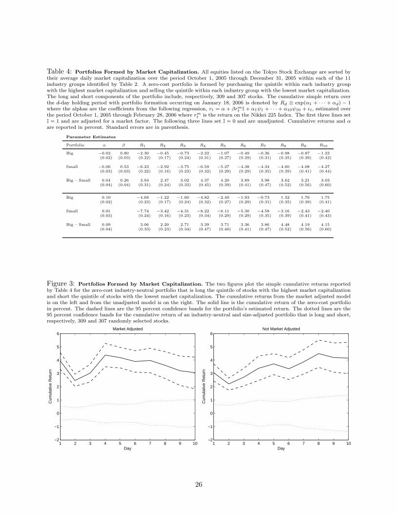
Table 4: Portfolios Formed by Market Capitalization. All equities listed on the Tokyo Stock Exchange are sorted bytheir average daily market capitalization over the period October 1, 2005 through December 31, 2005 within each of the 11industry groups identified by Table 2. A zero-cost portfolio is formed by purchasing the quintile within each industry groupwith the highest market capitalization and selling the quintile within each industry group with the lowest market capitalization.The long and short components of the portfolio include, respectively, 309 and 307 stocks. The cumulative simple return overthe d-day holding period with portfolio formation occurring on January 18, 2006 is denoted by Rd ≡ exp(α1 + · · · + αd) − 1where the alphas are the coefficients from the following regression, rt = α + βrm

t I + α1ψ1 + · · · + α10ψ10 + ǫt, estimated overthe period October 1, 2005 through February 28, 2006 where rm

t is the return on the Nikkei 225 Index. The first three lines setI = 1 and are adjusted for a market factor. The following three lines set I = 0 and are unadjusted. Cumulative returns and α

are reported in percent. Standard errors are in parenthesis.

Parameter Estimates

Portfolio α β R1 R2 R3 R4 R5 R6 R7 R8 R9 R10

Big −0.02 0.80 −2.30 −0.45 −0.73 −2.22 −1.07 −0.49 −0.36 −0.98 −0.87 −1.23(0.02) (0.03) (0.22) (0.17) (0.24) (0.31) (0.27) (0.29) (0.31) (0.35) (0.39) (0.42)

Small −0.06 0.53 −6.23 −2.92 −3.75 −6.59 −5.27 −4.38 −4.34 −4.60 −4.08 −4.27(0.03) (0.03) (0.22) (0.16) (0.23) (0.32) (0.29) (0.29) (0.35) (0.39) (0.41) (0.44)

Big – Small 0.04 0.26 3.94 2.47 3.02 4.37 4.20 3.89 3.98 3.62 3.21 3.03(0.04) (0.04) (0.31) (0.24) (0.33) (0.45) (0.39) (0.41) (0.47) (0.52) (0.56) (0.60)

Big 0.10 −4.68 −1.22 −1.60 −4.82 −2.40 −1.93 −0.73 1.32 1.76 1.75(0.02) (0.23) (0.17) (0.24) (0.32) (0.27) (0.29) (0.31) (0.35) (0.39) (0.41)

Small 0.01 −7.74 −3.42 −4.31 −8.22 −6.11 −5.30 −4.58 −3.16 −2.43 −2.40(0.03) (0.24) (0.16) (0.23) (0.34) (0.29) (0.29) (0.35) (0.39) (0.41) (0.43)

Big – Small 0.09 3.06 2.20 2.71 3.39 3.71 3.36 3.86 4.48 4.19 4.15(0.04) (0.33) (0.23) (0.34) (0.47) (0.40) (0.41) (0.47) (0.52) (0.56) (0.60)

Figure 3: Portfolios Formed by Market Capitalization. The two figures plot the simple cumulative returns reportedby Table 4 for the zero-cost industry-neutral portfolio that is long the quintile of stocks with the highest market capitalizationand short the quintile of stocks with the lowest market capitalization. The cumulative returns from the market adjusted modelis on the left and from the unadjusted model is on the right. The solid line is the cumulative return of the zero-cost portfolioin percent. The dashed lines are the 95 percent confidence bands for the portfolio’s estimated return. The dotted lines are the95 percent confidence bands for the cumulative return of an industry-neutral and size-adjusted portfolio that is long and short,respectively, 309 and 307 randomly selected stocks.

1 2 3 4 5 6 7 8 9 10−2

−1

0

1

2

3

4

5

6

Day

Cum

ulat

ive

Ret

urn

Market Adjusted

1 2 3 4 5 6 7 8 9 10−2

−1

0

1

2

3

4

5

6

Day

Cum

ulat

ive

Ret

urn

Not Market Adjusted

26

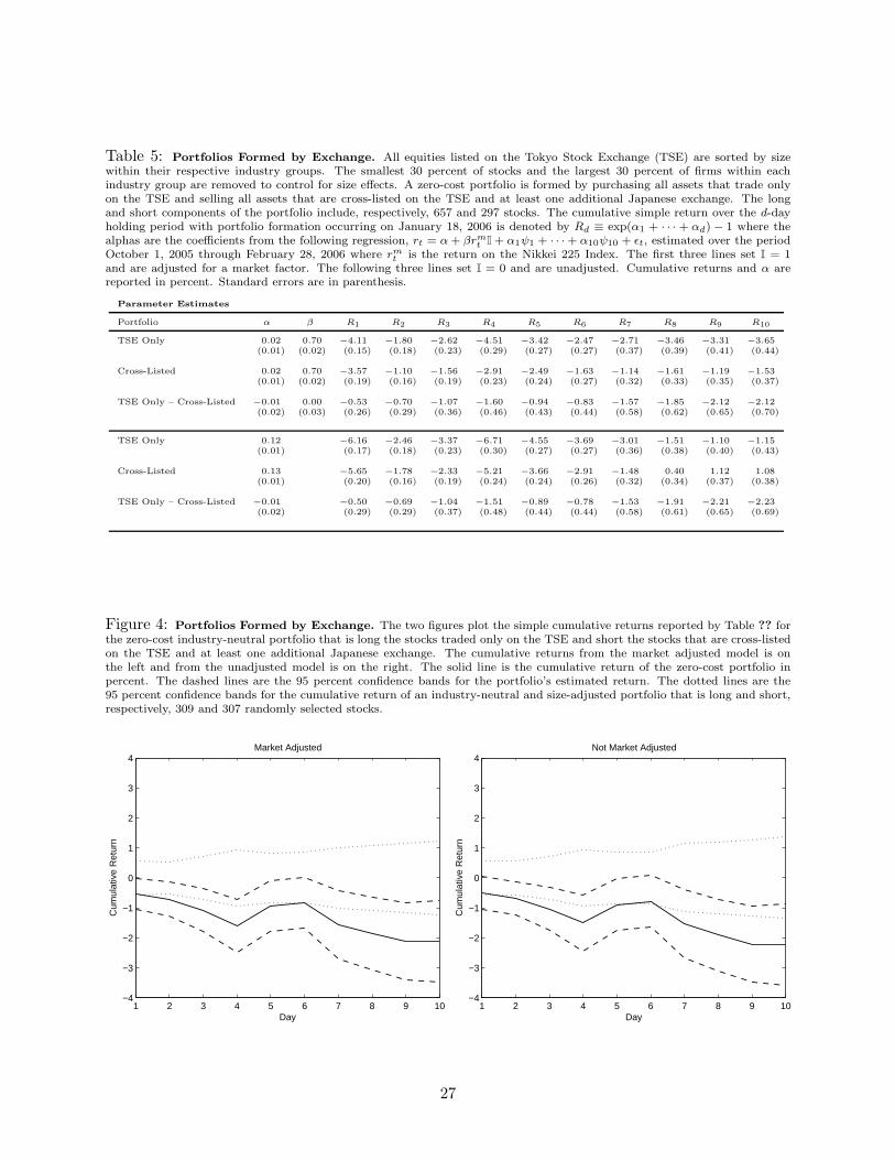
Table 5: Portfolios Formed by Exchange. All equities listed on the Tokyo Stock Exchange (TSE) are sorted by sizewithin their respective industry groups. The smallest 30 percent of stocks and the largest 30 percent of firms within eachindustry group are removed to control for size effects. A zero-cost portfolio is formed by purchasing all assets that trade onlyon the TSE and selling all assets that are cross-listed on the TSE and at least one additional Japanese exchange. The longand short components of the portfolio include, respectively, 657 and 297 stocks. The cumulative simple return over the d-dayholding period with portfolio formation occurring on January 18, 2006 is denoted by Rd ≡ exp(α1 + · · · + αd) − 1 where thealphas are the coefficients from the following regression, rt = α+ βrm

t I + α1ψ1 + · · · + α10ψ10 + ǫt, estimated over the periodOctober 1, 2005 through February 28, 2006 where rm

t is the return on the Nikkei 225 Index. The first three lines set I = 1and are adjusted for a market factor. The following three lines set I = 0 and are unadjusted. Cumulative returns and α arereported in percent. Standard errors are in parenthesis.

Parameter Estimates


TSE Only 0.02 0.70 −4.11 −1.80 −2.62 −4.51 −3.42 −2.47 −2.71 −3.46 −3.31 −3.65(0.01) (0.02) (0.15) (0.18) (0.23) (0.29) (0.27) (0.27) (0.37) (0.39) (0.41) (0.44)

Cross-Listed 0.02 0.70 −3.57 −1.10 −1.56 −2.91 −2.49 −1.63 −1.14 −1.61 −1.19 −1.53(0.01) (0.02) (0.19) (0.16) (0.19) (0.23) (0.24) (0.27) (0.32) (0.33) (0.35) (0.37)

TSE Only – Cross-Listed −0.01 0.00 −0.53 −0.70 −1.07 −1.60 −0.94 −0.83 −1.57 −1.85 −2.12 −2.12(0.02) (0.03) (0.26) (0.29) (0.36) (0.46) (0.43) (0.44) (0.58) (0.62) (0.65) (0.70)

TSE Only 0.12 −6.16 −2.46 −3.37 −6.71 −4.55 −3.69 −3.01 −1.51 −1.10 −1.15(0.01) (0.17) (0.18) (0.23) (0.30) (0.27) (0.27) (0.36) (0.38) (0.40) (0.43)

Cross-Listed 0.13 −5.65 −1.78 −2.33 −5.21 −3.66 −2.91 −1.48 0.40 1.12 1.08(0.01) (0.20) (0.16) (0.19) (0.24) (0.24) (0.26) (0.32) (0.34) (0.37) (0.38)

TSE Only – Cross-Listed −0.01 −0.50 −0.69 −1.04 −1.51 −0.89 −0.78 −1.53 −1.91 −2.21 −2.23(0.02) (0.29) (0.29) (0.37) (0.48) (0.44) (0.44) (0.58) (0.61) (0.65) (0.69)

Figure 4: Portfolios Formed by Exchange. The two figures plot the simple cumulative returns reported by Table ?? forthe zero-cost industry-neutral portfolio that is long the stocks traded only on the TSE and short the stocks that are cross-listedon the TSE and at least one additional Japanese exchange. The cumulative returns from the market adjusted model is onthe left and from the unadjusted model is on the right. The solid line is the cumulative return of the zero-cost portfolio inpercent. The dashed lines are the 95 percent confidence bands for the portfolio’s estimated return. The dotted lines are the95 percent confidence bands for the cumulative return of an industry-neutral and size-adjusted portfolio that is long and short,respectively, 309 and 307 randomly selected stocks.

1 2 3 4 5 6 7 8 9 10−4

−3

−2

−1

0

1

2

3

4

Day

Cum

ulat

ive

Ret

urn

Market Adjusted

1 2 3 4 5 6 7 8 9 10−4

−3

−2

−1

0

1

2

3

4

Day

Cum

ulat

ive

Ret

urn

Not Market Adjusted

27

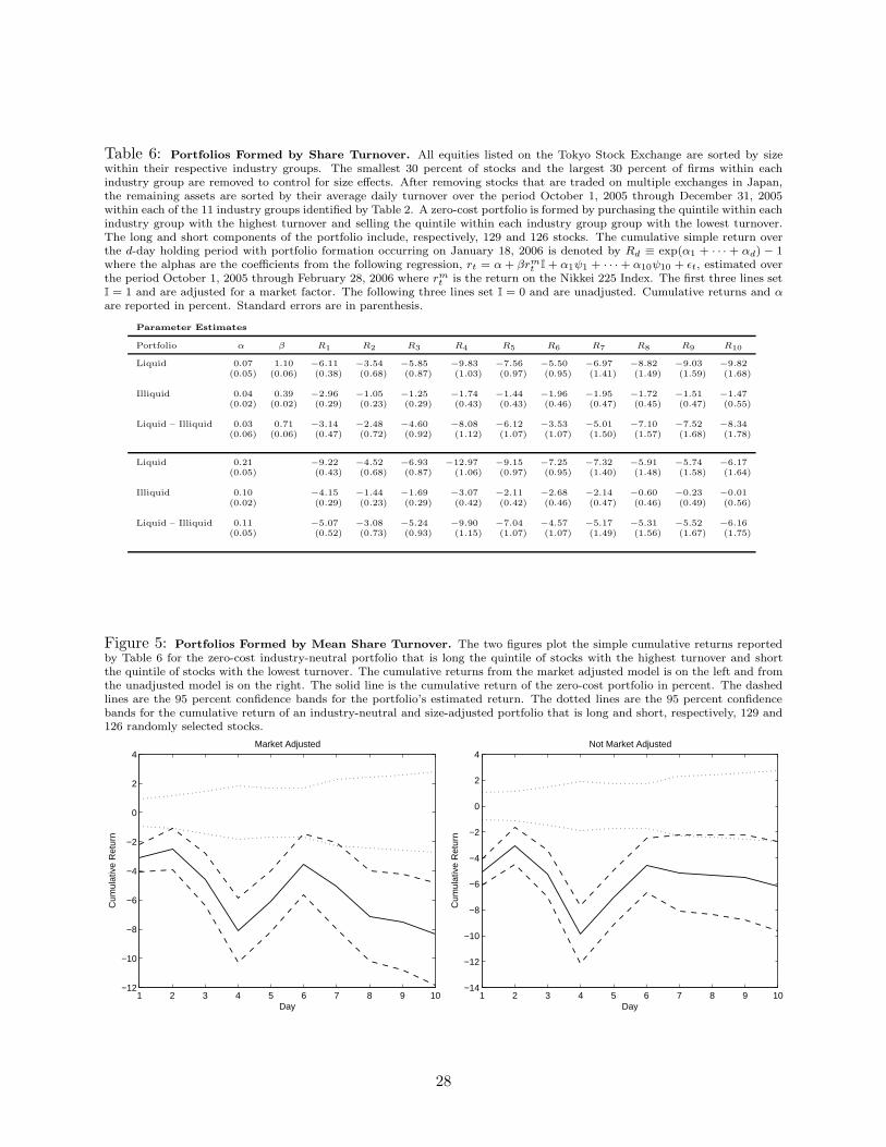
Table 6: Portfolios Formed by Share Turnover. All equities listed on the Tokyo Stock Exchange are sorted by sizewithin their respective industry groups. The smallest 30 percent of stocks and the largest 30 percent of firms within eachindustry group are removed to control for size effects. After removing stocks that are traded on multiple exchanges in Japan,the remaining assets are sorted by their average daily turnover over the period October 1, 2005 through December 31, 2005within each of the 11 industry groups identified by Table 2. A zero-cost portfolio is formed by purchasing the quintile within eachindustry group with the highest turnover and selling the quintile within each industry group group with the lowest turnover.The long and short components of the portfolio include, respectively, 129 and 126 stocks. The cumulative simple return overthe d-day holding period with portfolio formation occurring on January 18, 2006 is denoted by Rd ≡ exp(α1 + · · · + αd) − 1where the alphas are the coefficients from the following regression, rt = α + βrm




Parameter Estimates


Liquid 0.07 1.10 −6.11 −3.54 −5.85 −9.83 −7.56 −5.50 −6.97 −8.82 −9.03 −9.82(0.05) (0.06) (0.38) (0.68) (0.87) (1.03) (0.97) (0.95) (1.41) (1.49) (1.59) (1.68)

Illiquid 0.04 0.39 −2.96 −1.05 −1.25 −1.74 −1.44 −1.96 −1.95 −1.72 −1.51 −1.47(0.02) (0.02) (0.29) (0.23) (0.29) (0.43) (0.43) (0.46) (0.47) (0.45) (0.47) (0.55)

Liquid – Illiquid 0.03 0.71 −3.14 −2.48 −4.60 −8.08 −6.12 −3.53 −5.01 −7.10 −7.52 −8.34(0.06) (0.06) (0.47) (0.72) (0.92) (1.12) (1.07) (1.07) (1.50) (1.57) (1.68) (1.78)

Liquid 0.21 −9.22 −4.52 −6.93 −12.97 −9.15 −7.25 −7.32 −5.91 −5.74 −6.17(0.05) (0.43) (0.68) (0.87) (1.06) (0.97) (0.95) (1.40) (1.48) (1.58) (1.64)

Illiquid 0.10 −4.15 −1.44 −1.69 −3.07 −2.11 −2.68 −2.14 −0.60 −0.23 −0.01(0.02) (0.29) (0.23) (0.29) (0.42) (0.42) (0.46) (0.47) (0.46) (0.49) (0.56)

Liquid – Illiquid 0.11 −5.07 −3.08 −5.24 −9.90 −7.04 −4.57 −5.17 −5.31 −5.52 −6.16(0.05) (0.52) (0.73) (0.93) (1.15) (1.07) (1.07) (1.49) (1.56) (1.67) (1.75)

Figure 5: Portfolios Formed by Mean Share Turnover. The two figures plot the simple cumulative returns reportedby Table 6 for the zero-cost industry-neutral portfolio that is long the quintile of stocks with the highest turnover and shortthe quintile of stocks with the lowest turnover. The cumulative returns from the market adjusted model is on the left and fromthe unadjusted model is on the right. The solid line is the cumulative return of the zero-cost portfolio in percent. The dashedlines are the 95 percent confidence bands for the portfolio’s estimated return. The dotted lines are the 95 percent confidencebands for the cumulative return of an industry-neutral and size-adjusted portfolio that is long and short, respectively, 129 and126 randomly selected stocks.

1 2 3 4 5 6 7 8 9 10−12

−10

−8

−6

−4

−2

0

2

4

Day

Cum

ulat

ive

Ret

urn

Market Adjusted

1 2 3 4 5 6 7 8 9 10−14

−12

−10

−8

−6

−4

−2

0

2

4

Day

Cum

ulat

ive

Ret

urn

Not Market Adjusted

28

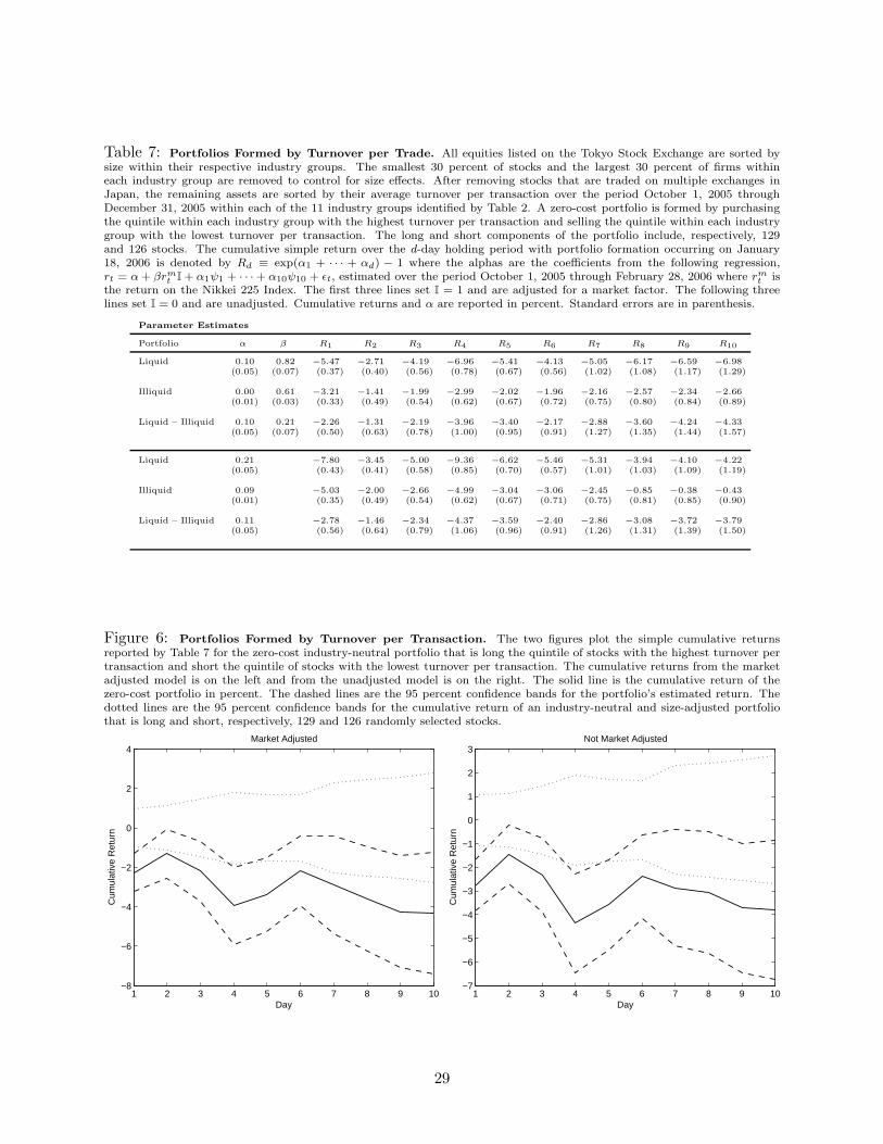
Table 7: Portfolios Formed by Turnover per Trade. All equities listed on the Tokyo Stock Exchange are sorted bysize within their respective industry groups. The smallest 30 percent of stocks and the largest 30 percent of firms withineach industry group are removed to control for size effects. After removing stocks that are traded on multiple exchanges inJapan, the remaining assets are sorted by their average turnover per transaction over the period October 1, 2005 throughDecember 31, 2005 within each of the 11 industry groups identified by Table 2. A zero-cost portfolio is formed by purchasingthe quintile within each industry group with the highest turnover per transaction and selling the quintile within each industrygroup with the lowest turnover per transaction. The long and short components of the portfolio include, respectively, 129and 126 stocks. The cumulative simple return over the d-day holding period with portfolio formation occurring on January18, 2006 is denoted by Rd ≡ exp(α1 + · · · + αd) − 1 where the alphas are the coefficients from the following regression,rt = α+ βrm

t I + α1ψ1 + · · · + α10ψ10 + ǫt, estimated over the period October 1, 2005 through February 28, 2006 where rmt is

the return on the Nikkei 225 Index. The first three lines set I = 1 and are adjusted for a market factor. The following threelines set I = 0 and are unadjusted. Cumulative returns and α are reported in percent. Standard errors are in parenthesis.

Parameter Estimates


Liquid 0.10 0.82 −5.47 −2.71 −4.19 −6.96 −5.41 −4.13 −5.05 −6.17 −6.59 −6.98(0.05) (0.07) (0.37) (0.40) (0.56) (0.78) (0.67) (0.56) (1.02) (1.08) (1.17) (1.29)

Illiquid 0.00 0.61 −3.21 −1.41 −1.99 −2.99 −2.02 −1.96 −2.16 −2.57 −2.34 −2.66(0.01) (0.03) (0.33) (0.49) (0.54) (0.62) (0.67) (0.72) (0.75) (0.80) (0.84) (0.89)

Liquid – Illiquid 0.10 0.21 −2.26 −1.31 −2.19 −3.96 −3.40 −2.17 −2.88 −3.60 −4.24 −4.33(0.05) (0.07) (0.50) (0.63) (0.78) (1.00) (0.95) (0.91) (1.27) (1.35) (1.44) (1.57)

Liquid 0.21 −7.80 −3.45 −5.00 −9.36 −6.62 −5.46 −5.31 −3.94 −4.10 −4.22(0.05) (0.43) (0.41) (0.58) (0.85) (0.70) (0.57) (1.01) (1.03) (1.09) (1.19)

Illiquid 0.09 −5.03 −2.00 −2.66 −4.99 −3.04 −3.06 −2.45 −0.85 −0.38 −0.43(0.01) (0.35) (0.49) (0.54) (0.62) (0.67) (0.71) (0.75) (0.81) (0.85) (0.90)

Liquid – Illiquid 0.11 −2.78 −1.46 −2.34 −4.37 −3.59 −2.40 −2.86 −3.08 −3.72 −3.79(0.05) (0.56) (0.64) (0.79) (1.06) (0.96) (0.91) (1.26) (1.31) (1.39) (1.50)

Figure 6: Portfolios Formed by Turnover per Transaction. The two figures plot the simple cumulative returnsreported by Table 7 for the zero-cost industry-neutral portfolio that is long the quintile of stocks with the highest turnover pertransaction and short the quintile of stocks with the lowest turnover per transaction. The cumulative returns from the marketadjusted model is on the left and from the unadjusted model is on the right. The solid line is the cumulative return of thezero-cost portfolio in percent. The dashed lines are the 95 percent confidence bands for the portfolio’s estimated return. Thedotted lines are the 95 percent confidence bands for the cumulative return of an industry-neutral and size-adjusted portfoliothat is long and short, respectively, 129 and 126 randomly selected stocks.

1 2 3 4 5 6 7 8 9 10−8

−6

−4

−2

0

2

4

Day

Cum

ulat

ive

Ret

urn

Market Adjusted

1 2 3 4 5 6 7 8 9 10−7

−6

−5

−4

−3

−2

−1

0

1

2

3

Day

Cum

ulat

ive

Ret

urn

Not Market Adjusted

29

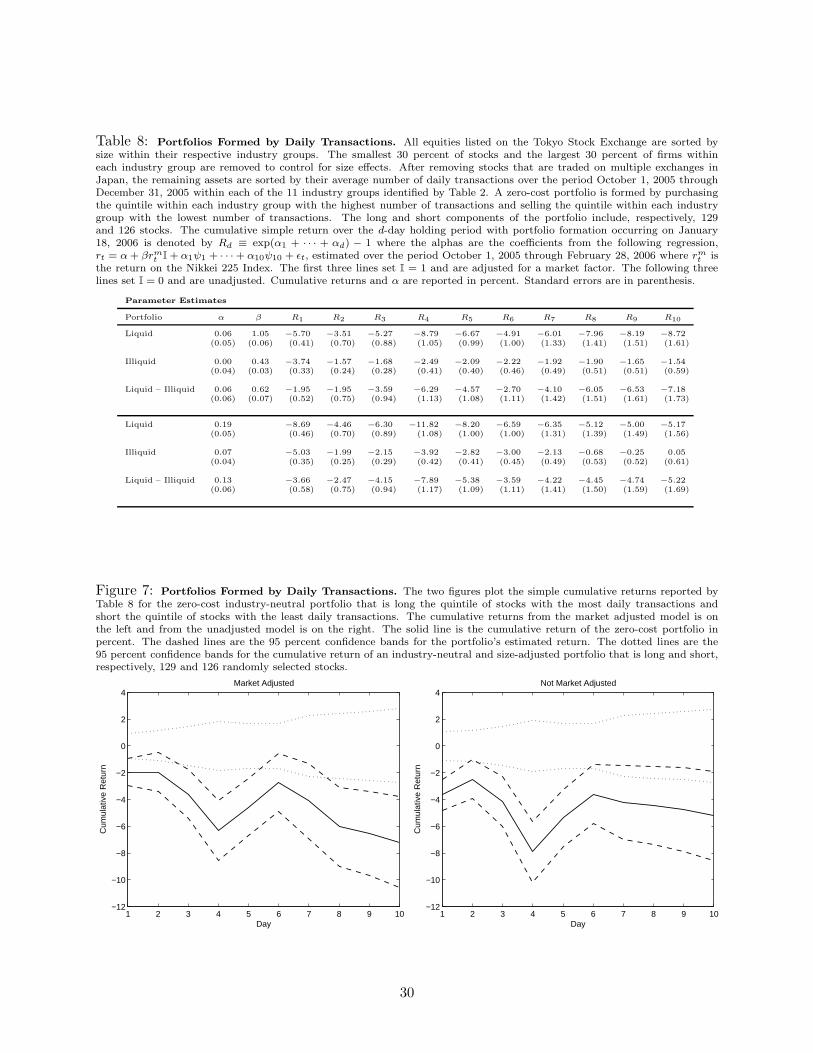
Table 8: Portfolios Formed by Daily Transactions. All equities listed on the Tokyo Stock Exchange are sorted bysize within their respective industry groups. The smallest 30 percent of stocks and the largest 30 percent of firms withineach industry group are removed to control for size effects. After removing stocks that are traded on multiple exchanges inJapan, the remaining assets are sorted by their average number of daily transactions over the period October 1, 2005 throughDecember 31, 2005 within each of the 11 industry groups identified by Table 2. A zero-cost portfolio is formed by purchasingthe quintile within each industry group with the highest number of transactions and selling the quintile within each industrygroup with the lowest number of transactions. The long and short components of the portfolio include, respectively, 129and 126 stocks. The cumulative simple return over the d-day holding period with portfolio formation occurring on January18, 2006 is denoted by Rd ≡ exp(α1 + · · · + αd) − 1 where the alphas are the coefficients from the following regression,rt = α+ βrm



Parameter Estimates


Liquid 0.06 1.05 −5.70 −3.51 −5.27 −8.79 −6.67 −4.91 −6.01 −7.96 −8.19 −8.72(0.05) (0.06) (0.41) (0.70) (0.88) (1.05) (0.99) (1.00) (1.33) (1.41) (1.51) (1.61)

Illiquid 0.00 0.43 −3.74 −1.57 −1.68 −2.49 −2.09 −2.22 −1.92 −1.90 −1.65 −1.54(0.04) (0.03) (0.33) (0.24) (0.28) (0.41) (0.40) (0.46) (0.49) (0.51) (0.51) (0.59)

Liquid – Illiquid 0.06 0.62 −1.95 −1.95 −3.59 −6.29 −4.57 −2.70 −4.10 −6.05 −6.53 −7.18(0.06) (0.07) (0.52) (0.75) (0.94) (1.13) (1.08) (1.11) (1.42) (1.51) (1.61) (1.73)

Liquid 0.19 −8.69 −4.46 −6.30 −11.82 −8.20 −6.59 −6.35 −5.12 −5.00 −5.17(0.05) (0.46) (0.70) (0.89) (1.08) (1.00) (1.00) (1.31) (1.39) (1.49) (1.56)

Illiquid 0.07 −5.03 −1.99 −2.15 −3.92 −2.82 −3.00 −2.13 −0.68 −0.25 0.05(0.04) (0.35) (0.25) (0.29) (0.42) (0.41) (0.45) (0.49) (0.53) (0.52) (0.61)

Liquid – Illiquid 0.13 −3.66 −2.47 −4.15 −7.89 −5.38 −3.59 −4.22 −4.45 −4.74 −5.22(0.06) (0.58) (0.75) (0.94) (1.17) (1.09) (1.11) (1.41) (1.50) (1.59) (1.69)

Figure 7: Portfolios Formed by Daily Transactions. The two figures plot the simple cumulative returns reported byTable 8 for the zero-cost industry-neutral portfolio that is long the quintile of stocks with the most daily transactions andshort the quintile of stocks with the least daily transactions. The cumulative returns from the market adjusted model is onthe left and from the unadjusted model is on the right. The solid line is the cumulative return of the zero-cost portfolio inpercent. The dashed lines are the 95 percent confidence bands for the portfolio’s estimated return. The dotted lines are the95 percent confidence bands for the cumulative return of an industry-neutral and size-adjusted portfolio that is long and short,respectively, 129 and 126 randomly selected stocks.

1 2 3 4 5 6 7 8 9 10−12

−10

−8

−6

−4

−2

0

2

4

Day

Cum

ulat

ive

Ret

urn

Market Adjusted

1 2 3 4 5 6 7 8 9 10−12

−10

−8

−6

−4

−2

0

2

4

Day

Cum

ulat

ive

Ret

urn

Not Market Adjusted

30

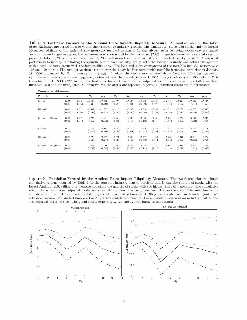
Table 9: Portfolios Formed by the Amihud Price Impact Illiquidity Measure. All equities listed on the TokyoStock Exchange are sorted by size within their respective industry groups. The smallest 30 percent of stocks and the largest30 percent of firms within each industry group are removed to control for size effects. After removing stocks that are tradedon multiple exchanges in Japan, the remaining assets are sorted by their Amihud (2002) illiquidity measure calculated over theperiod October 1, 2005 through December 31, 2005 within each of the 11 industry groups identified by Table 2. A zero-costportfolio is formed by purchasing the quintile within each industry group with the lowest illiquidity and selling the quintilewithin each industry group with the highest illiquidity. The long and short components of the portfolio include, respectively,126 and 129 stocks. The cumulative simple return over the d-day holding period with portfolio formation occurring on January18, 2006 is denoted by Rd ≡ exp(α1 + · · · + αd) − 1 where the alphas are the coefficients from the following regression,rt = α+ βrm



Parameter Estimates


Liquid 0.05 0.99 −4.93 −2.98 −4.73 −7.66 −5.99 −4.30 −5.33 −7.00 −7.25 −7.95(0.04) (0.06) (0.39) (0.69) (0.86) (1.04) (0.99) (0.98) (1.34) (1.42) (1.51) (1.55)

Illiquid 0.00 0.51 −3.68 −1.57 −2.15 −3.36 −2.63 −2.62 −2.54 −2.77 −2.37 −2.60(0.05) (0.04) (0.34) (0.27) (0.38) (0.53) (0.50) (0.52) (0.55) (0.56) (0.63) (0.67)

Liquid – Illiquid 0.05 0.47 −1.25 −1.41 −2.58 −4.30 −3.36 −1.68 −2.79 −4.24 −4.88 −5.35(0.06) (0.07) (0.52) (0.73) (0.94) (1.16) (1.10) (1.10) (1.44) (1.52) (1.62) (1.68)

Liquid 0.17 −7.75 −3.86 −5.70 −10.52 −7.43 −5.88 −5.64 −4.34 −4.25 −4.58(0.04) (0.47) (0.69) (0.87) (1.08) (1.01) (0.98) (1.33) (1.41) (1.50) (1.54)

Illiquid 0.08 −5.20 −2.07 −2.71 −5.02 −3.47 −3.54 −2.78 −1.31 −0.71 −0.72(0.04) (0.36) (0.27) (0.38) (0.55) (0.50) (0.51) (0.54) (0.57) (0.63) (0.68)

Liquid – Illiquid 0.10 −2.55 −1.79 −2.99 −5.50 −3.95 −2.34 −2.86 −3.03 −3.54 −3.86(0.06) (0.59) (0.74) (0.94) (1.20) (1.11) (1.10) (1.43) (1.51) (1.61) (1.67)

Figure 8: Portfolios Formed by the Amihud Price Impact Illiquidity Measure. The two figures plot the simplecumulative returns reported by Table 9 for the zero-cost industry-neutral portfolio that is long the quintile of stocks with thelowest Amihud (2002) illiquidity measure and short the quintile of stocks with the highest illiquidity measure. The cumulativereturns from the market adjusted model is on the left and from the unadjusted model is on the right. The solid line is thecumulative return of the zero-cost portfolio in percent. The dashed lines are the 95 percent confidence bands for the portfolio’sestimated return. The dotted lines are the 95 percent confidence bands for the cumulative return of an industry-neutral andsize-adjusted portfolio that is long and short, respectively, 126 and 129 randomly selected stocks.

1 2 3 4 5 6 7 8 9 10−10

−8

−6

−4

−2

0

2

4

Day

Cum

ulat

ive

Ret

urn

Market Adjusted

1 2 3 4 5 6 7 8 9 10−8

−6

−4

−2

0

2

4

Day

Cum

ulat

ive

Ret

urn

Not Market Adjusted

31

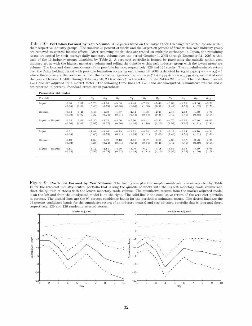
Table 10: Portfolios Formed by Yen Volume. All equities listed on the Tokyo Stock Exchange are sorted by size withintheir respective industry groups. The smallest 30 percent of stocks and the largest 30 percent of firms within each industry groupare removed to control for size effects. After removing stocks that are traded on multiple exchanges in Japan, the remainingassets are sorted by their average daily monetary volume over the period October 1, 2005 through December 31, 2005 withineach of the 11 industry groups identified by Table 2. A zero-cost portfolio is formed by purchasing the quintile within eachindustry group with the highest monetary volume and selling the quintile within each industry group with the lowest monetaryvolume. The long and short components of the portfolio include, respectively, 129 and 126 stocks. The cumulative simple returnover the d-day holding period with portfolio formation occurring on January 18, 2006 is denoted by Rd ≡ exp(α1 + · · ·+αd)−1where the alphas are the coefficients from the following regression, rt = α + βrm




Parameter Estimates


Liquid 0.08 1.07 −5.76 −3.64 −5.68 −9.44 −7.39 −5.49 −6.88 −8.79 −9.06 −9.76(0.05) (0.06) (0.40) (0.73) (0.90) (1.06) (1.00) (0.99) (1.44) (1.52) (1.62) (1.71)

Illiquid 0.04 0.41 −3.46 −1.39 −1.67 −2.44 −1.98 −2.27 −2.18 −2.13 −1.60 −1.77(0.02) (0.02) (0.32) (0.24) (0.31) (0.44) (0.44) (0.46) (0.47) (0.45) (0.48) (0.54)

Liquid – Illiquid 0.04 0.66 −2.30 −2.25 −4.00 −7.00 −5.41 −3.22 −4.70 −6.66 −7.46 −8.00(0.06) (0.07) (0.52) (0.77) (0.96) (1.16) (1.10) (1.10) (1.53) (1.60) (1.71) (1.82)

Liquid 0.21 −8.81 −4.60 −6.73 −12.51 −8.94 −7.19 −7.22 −5.94 −5.86 −6.21(0.05) (0.46) (0.73) (0.91) (1.09) (1.01) (1.00) (1.43) (1.51) (1.61) (1.68)

Illiquid 0.10 −4.69 −1.79 −2.13 −3.81 −2.67 −3.01 −2.38 −0.97 −0.26 −0.25(0.02) (0.33) (0.24) (0.31) (0.44) (0.44) (0.46) (0.47) (0.45) (0.49) (0.55)

Liquid – Illiquid 0.11 −4.12 −2.81 −4.60 −8.70 −6.27 −4.18 −4.84 −4.98 −5.59 −5.96(0.05) (0.57) (0.78) (0.97) (1.19) (1.11) (1.10) (1.52) (1.59) (1.69) (1.78)

Figure 9: Portfolios Formed by Yen Volume. The two figures plot the simple cumulative returns reported by Table10 for the zero-cost industry-neutral portfolio that is long the quintile of stocks with the highest monetary trade volume andshort the quintile of stocks with the lowest monetary trade volume. The cumulative returns from the market adjusted modelis on the left and from the unadjusted model is on the right. The solid line is the cumulative return of the zero-cost portfolioin percent. The dashed lines are the 95 percent confidence bands for the portfolio’s estimated return. The dotted lines are the95 percent confidence bands for the cumulative return of an industry-neutral and size-adjusted portfolio that is long and short,respectively, 129 and 126 randomly selected stocks.

1 2 3 4 5 6 7 8 9 10−12

−10

−8

−6

−4

−2

0

2

4

Day

Cum

ulat

ive

Ret

urn

Market Adjusted

1 2 3 4 5 6 7 8 9 10−12

−10

−8

−6

−4

−2

0

2

4

Day

Cum

ulat

ive

Ret

urn

Not Market Adjusted

32

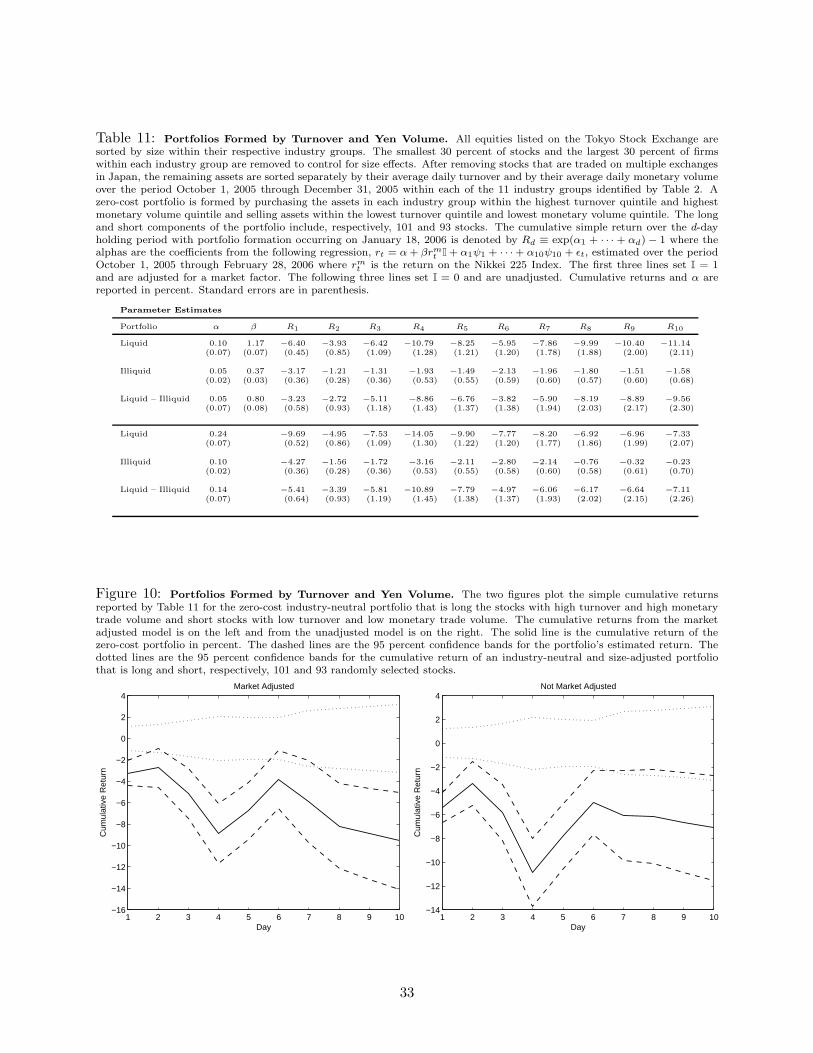
Table 11: Portfolios Formed by Turnover and Yen Volume. All equities listed on the Tokyo Stock Exchange aresorted by size within their respective industry groups. The smallest 30 percent of stocks and the largest 30 percent of firmswithin each industry group are removed to control for size effects. After removing stocks that are traded on multiple exchangesin Japan, the remaining assets are sorted separately by their average daily turnover and by their average daily monetary volumeover the period October 1, 2005 through December 31, 2005 within each of the 11 industry groups identified by Table 2. Azero-cost portfolio is formed by purchasing the assets in each industry group within the highest turnover quintile and highestmonetary volume quintile and selling assets within the lowest turnover quintile and lowest monetary volume quintile. The longand short components of the portfolio include, respectively, 101 and 93 stocks. The cumulative simple return over the d-dayholding period with portfolio formation occurring on January 18, 2006 is denoted by Rd ≡ exp(α1 + · · · + αd) − 1 where thealphas are the coefficients from the following regression, rt = α+ βrm

t I + α1ψ1 + · · · + α10ψ10 + ǫt, estimated over the periodOctober 1, 2005 through February 28, 2006 where rm

t is the return on the Nikkei 225 Index. The first three lines set I = 1and are adjusted for a market factor. The following three lines set I = 0 and are unadjusted. Cumulative returns and α arereported in percent. Standard errors are in parenthesis.

Parameter Estimates


Liquid 0.10 1.17 −6.40 −3.93 −6.42 −10.79 −8.25 −5.95 −7.86 −9.99 −10.40 −11.14(0.07) (0.07) (0.45) (0.85) (1.09) (1.28) (1.21) (1.20) (1.78) (1.88) (2.00) (2.11)

Illiquid 0.05 0.37 −3.17 −1.21 −1.31 −1.93 −1.49 −2.13 −1.96 −1.80 −1.51 −1.58(0.02) (0.03) (0.36) (0.28) (0.36) (0.53) (0.55) (0.59) (0.60) (0.57) (0.60) (0.68)

Liquid – Illiquid 0.05 0.80 −3.23 −2.72 −5.11 −8.86 −6.76 −3.82 −5.90 −8.19 −8.89 −9.56(0.07) (0.08) (0.58) (0.93) (1.18) (1.43) (1.37) (1.38) (1.94) (2.03) (2.17) (2.30)

Liquid 0.24 −9.69 −4.95 −7.53 −14.05 −9.90 −7.77 −8.20 −6.92 −6.96 −7.33(0.07) (0.52) (0.86) (1.09) (1.30) (1.22) (1.20) (1.77) (1.86) (1.99) (2.07)

Illiquid 0.10 −4.27 −1.56 −1.72 −3.16 −2.11 −2.80 −2.14 −0.76 −0.32 −0.23(0.02) (0.36) (0.28) (0.36) (0.53) (0.55) (0.58) (0.60) (0.58) (0.61) (0.70)

Liquid – Illiquid 0.14 −5.41 −3.39 −5.81 −10.89 −7.79 −4.97 −6.06 −6.17 −6.64 −7.11(0.07) (0.64) (0.93) (1.19) (1.45) (1.38) (1.37) (1.93) (2.02) (2.15) (2.26)

Figure 10: Portfolios Formed by Turnover and Yen Volume. The two figures plot the simple cumulative returnsreported by Table 11 for the zero-cost industry-neutral portfolio that is long the stocks with high turnover and high monetarytrade volume and short stocks with low turnover and low monetary trade volume. The cumulative returns from the marketadjusted model is on the left and from the unadjusted model is on the right. The solid line is the cumulative return of thezero-cost portfolio in percent. The dashed lines are the 95 percent confidence bands for the portfolio’s estimated return. Thedotted lines are the 95 percent confidence bands for the cumulative return of an industry-neutral and size-adjusted portfoliothat is long and short, respectively, 101 and 93 randomly selected stocks.

1 2 3 4 5 6 7 8 9 10−16

−14

−12

−10

−8

−6

−4

−2

0

2

4

Day

Cum

ulat

ive

Ret

urn

Market Adjusted

1 2 3 4 5 6 7 8 9 10−14

−12

−10

−8

−6

−4

−2

0

2

4

Day

Cum

ulat

ive

Ret

urn

Not Market Adjusted

33

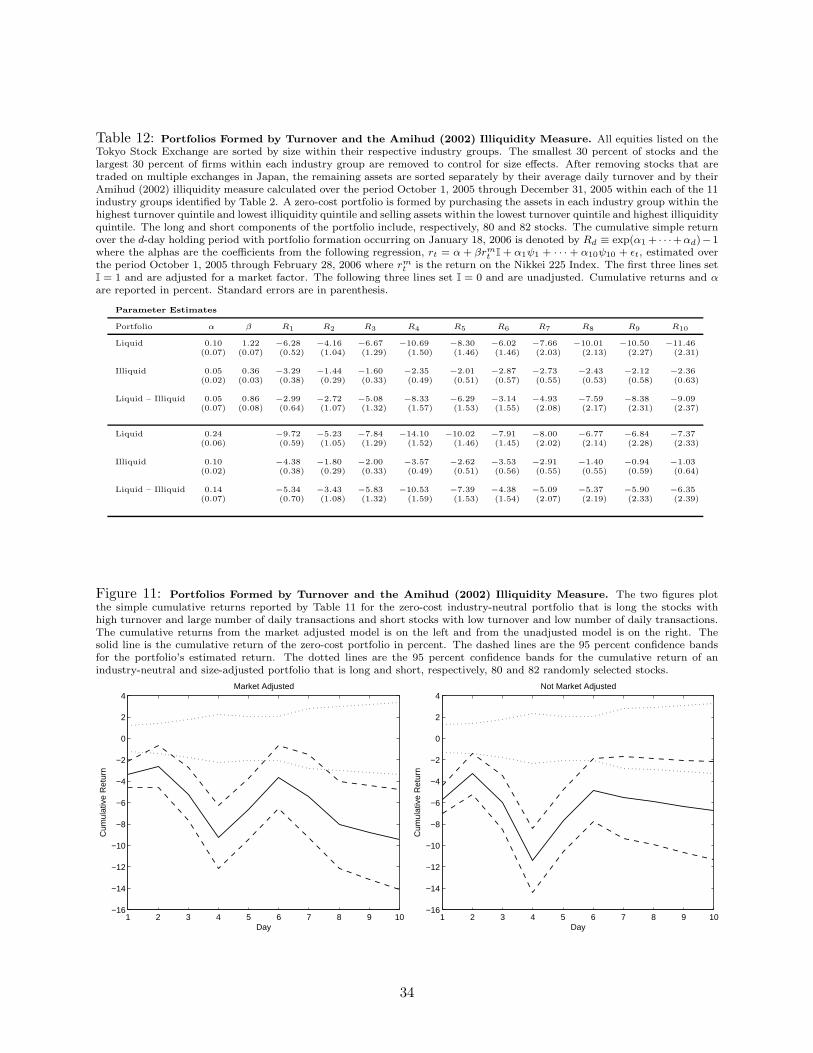
Table 12: Portfolios Formed by Turnover and the Amihud (2002) Illiquidity Measure. All equities listed on theTokyo Stock Exchange are sorted by size within their respective industry groups. The smallest 30 percent of stocks and thelargest 30 percent of firms within each industry group are removed to control for size effects. After removing stocks that aretraded on multiple exchanges in Japan, the remaining assets are sorted separately by their average daily turnover and by theirAmihud (2002) illiquidity measure calculated over the period October 1, 2005 through December 31, 2005 within each of the 11industry groups identified by Table 2. A zero-cost portfolio is formed by purchasing the assets in each industry group within thehighest turnover quintile and lowest illiquidity quintile and selling assets within the lowest turnover quintile and highest illiquidityquintile. The long and short components of the portfolio include, respectively, 80 and 82 stocks. The cumulative simple returnover the d-day holding period with portfolio formation occurring on January 18, 2006 is denoted by Rd ≡ exp(α1 + · · ·+αd)−1where the alphas are the coefficients from the following regression, rt = α + βrm




Parameter Estimates


Liquid 0.10 1.22 −6.28 −4.16 −6.67 −10.69 −8.30 −6.02 −7.66 −10.01 −10.50 −11.46(0.07) (0.07) (0.52) (1.04) (1.29) (1.50) (1.46) (1.46) (2.03) (2.13) (2.27) (2.31)

Illiquid 0.05 0.36 −3.29 −1.44 −1.60 −2.35 −2.01 −2.87 −2.73 −2.43 −2.12 −2.36(0.02) (0.03) (0.38) (0.29) (0.33) (0.49) (0.51) (0.57) (0.55) (0.53) (0.58) (0.63)

Liquid – Illiquid 0.05 0.86 −2.99 −2.72 −5.08 −8.33 −6.29 −3.14 −4.93 −7.59 −8.38 −9.09(0.07) (0.08) (0.64) (1.07) (1.32) (1.57) (1.53) (1.55) (2.08) (2.17) (2.31) (2.37)

Liquid 0.24 −9.72 −5.23 −7.84 −14.10 −10.02 −7.91 −8.00 −6.77 −6.84 −7.37(0.06) (0.59) (1.05) (1.29) (1.52) (1.46) (1.45) (2.02) (2.14) (2.28) (2.33)

Illiquid 0.10 −4.38 −1.80 −2.00 −3.57 −2.62 −3.53 −2.91 −1.40 −0.94 −1.03(0.02) (0.38) (0.29) (0.33) (0.49) (0.51) (0.56) (0.55) (0.55) (0.59) (0.64)

Liquid – Illiquid 0.14 −5.34 −3.43 −5.83 −10.53 −7.39 −4.38 −5.09 −5.37 −5.90 −6.35(0.07) (0.70) (1.08) (1.32) (1.59) (1.53) (1.54) (2.07) (2.19) (2.33) (2.39)

Figure 11: Portfolios Formed by Turnover and the Amihud (2002) Illiquidity Measure. The two figures plotthe simple cumulative returns reported by Table 11 for the zero-cost industry-neutral portfolio that is long the stocks withhigh turnover and large number of daily transactions and short stocks with low turnover and low number of daily transactions.The cumulative returns from the market adjusted model is on the left and from the unadjusted model is on the right. Thesolid line is the cumulative return of the zero-cost portfolio in percent. The dashed lines are the 95 percent confidence bandsfor the portfolio’s estimated return. The dotted lines are the 95 percent confidence bands for the cumulative return of anindustry-neutral and size-adjusted portfolio that is long and short, respectively, 80 and 82 randomly selected stocks.

1 2 3 4 5 6 7 8 9 10−16

−14

−12

−10

−8

−6

−4

−2

0

2

4

Day

Cum

ulat

ive

Ret

urn

Market Adjusted

1 2 3 4 5 6 7 8 9 10−16

−14

−12

−10

−8

−6

−4

−2

0

2

4

Day

Cum

ulat

ive

Ret

urn

Not Market Adjusted

34

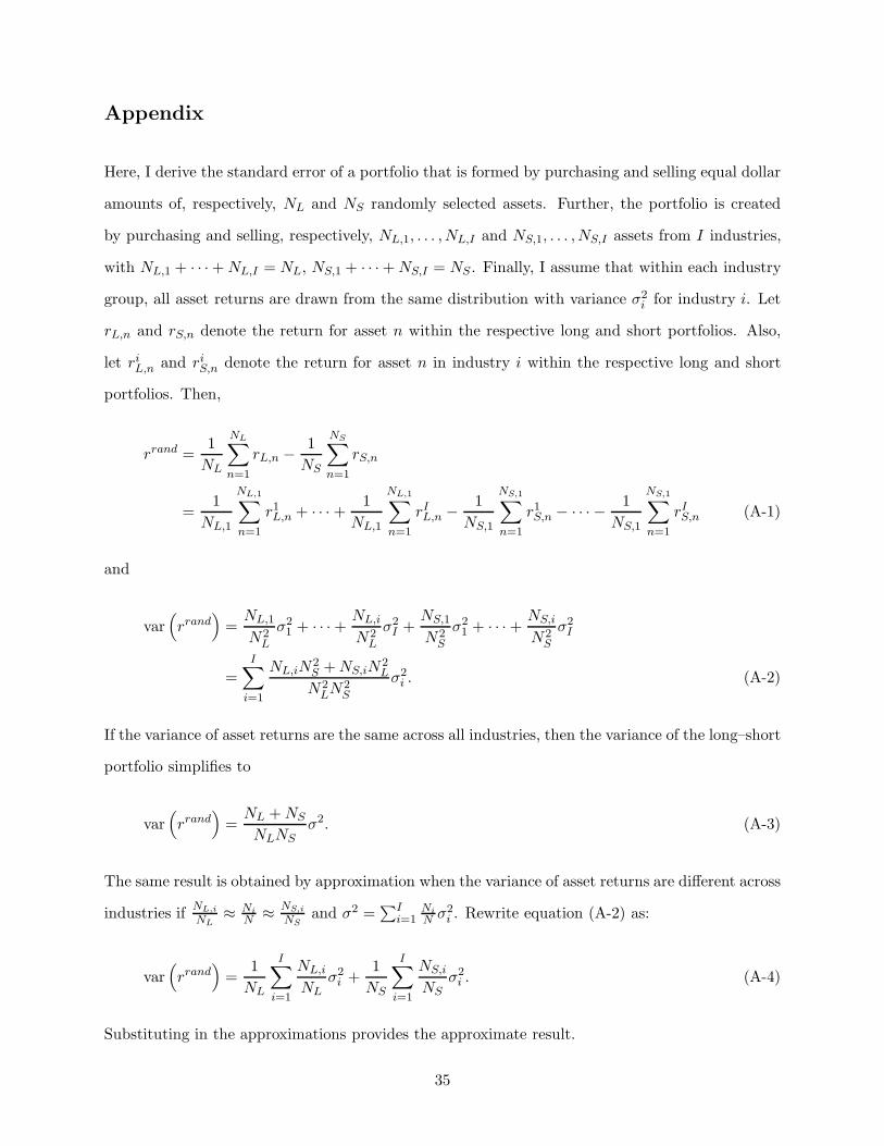
Appendix

Here, I derive the standard error of a portfolio that is formed by purchasing and selling equal dollar

amounts of, respectively, NL and NS randomly selected assets. Further, the portfolio is created

by purchasing and selling, respectively, NL,1, . . . , NL,I and NS,1, . . . , NS,I assets from I industries,

with NL,1 + · · · +NL,I = NL, NS,1 + · · · +NS,I = NS . Finally, I assume that within each industry

group, all asset returns are drawn from the same distribution with variance σ2i for industry i. Let

rL,n and rS,n denote the return for asset n within the respective long and short portfolios. Also,

let riL,n and riS,n denote the return for asset n in industry i within the respective long and short

portfolios. Then,

rrand =1

NL

NL∑

n=1

rL,n −1

NS

NS∑

n=1

rS,n

=1

NL,1

NL,1∑

n=1

r1L,n + · · · +1

NL,1

NL,1∑

n=1

rIL,n −1

NS,1

NS,1∑

n=1

r1S,n − · · · −1

NS,1

NS,1∑

n=1

rIS,n (A-1)

and

var(

rrand)

=NL,1

N2L

σ21 + · · · +

NL,i

N2L

σ2I +

NS,1

N2S

σ21 + · · · +

NS,i

N2S

σ2I

=I∑

i=1

NL,iN2S +NS,iN

2L

N2LN

2S

σ2i . (A-2)

If the variance of asset returns are the same across all industries, then the variance of the long–short

portfolio simplifies to

var(

rrand)

=NL +NS

NLNS

σ2. (A-3)

The same result is obtained by approximation when the variance of asset returns are different across

industries ifNL,i

NL≈ Ni

N≈

NS,i

NSand σ2 =

∑Ii=1

Ni

Nσ2i . Rewrite equation (A-2) as:

var(

rrand)

=1

NL

I∑

i=1

NL,i

NL

σ2i +

1

NS

I∑

i=1

NS,i

NS

σ2i . (A-4)

Substituting in the approximations provides the approximate result.

35

Surprise! It’s Illiquid: The January 2006 Tokyo Stock ...mkearns/finread/ronisurpise.pdf · The...

Documents

Transcript of Surprise! It’s Illiquid: The January 2006 Tokyo Stock ...mkearns/finread/ronisurpise.pdf · The...