iGrafx 2003 - User's Guide
226
• Modeling Activities • Editing Using the Tabular View • Describing Model Behavior • Running a Simulation • Using Trace Mode • Using Multiple Processes • Using Monitors • Reporting Results • Using Graphs • Index iGrafx Process 2000 User’s Guide iGrafx S Y S T E M License Agreement Copyright Information
-
Upload
richard-booy -
Category
Documents
-
view
138 -
download
18
Transcript of iGrafx 2003 - User's Guide

• Modeling Activities
• Editing Using the Tabular View
• Describing Model Behavior
• Running a Simulation
• Using Trace Mode
• Using Multiple Processes
• Using Monitors
• Reporting Results
• Using Graphs
• Index
iGrafx Process 2000 User’s Guide
iGrafxS Y S T E M
License Agreement
Copyright Information

Home Index Previous Page Next PageiGrafxS Y S T E M
� � � � � � � � � � � � � � � � 2
Modeling Activities
About Process Modeling
Process modeling is one of the most cost-effective and rewarding ideas to come along in years. It can help identify improvements and pinpoint errors before they occur. Statistics generated by process modeling can provide accurate numbers about cycle time, costs, problem areas, and bottlenecks. Some of the benefits of having these statistics available include gaining insight into processes, facilitating change, and enhancing communication within organizations.
If you picture a busy train station, you can imagine many of the dynamics of a process in action. As trains arrive and depart, the stationmasters are busy making routing and timing decisions. Meanwhile, passengers wait in line to buy tickets or to board.
Over time, the train operators gather and examine statistics. This includes such things as the average travel time between cities, the length of time that a train typically waits before departing, and how much fuel is used per mile. These types of statistics help guide future decisions.

Home Index Previous Page Next PageiGrafxS Y S T E M
� � � � � � � � � � � � � � � � 3
When you use modeling and simulation software, you simulate several weeks or months of activities within a matter of seconds. The results can help you make decisions to improve your processes or recommend changes. Of course, you can study the same choices by direct experimentation or by building prototypes. But a computer simulation can identify potential obstacles, problems, and threats to business opportunities in an efficient and effective way.
The process diagram is a series of activities, drawn as symbols, linked together with directed lines. An activity is an individual step of a process diagram. iGrafx Process 2000 represents an activity as a symbol in a flowchart.
About Models
Process activities have many different variations. The most common process activity is a duration, or time, that the activity takes. For example, an activity may take four hours (constant duration) or between one and two days (distributed duration).
Another typical activity is a decision point. If the process branches into different paths based on some percentage or a specification or production value, you set decision outputs for the activity.
Many models contain only activities that have duration and decision criteria. Often, you do not need anything more complex. In the following example, the activities labeled Duration take a set amount of time and the Decision activity branches depending on a set percentage.

Home Index Previous Page Next PageiGrafxS Y S T E M
� � � � � � � � � � � � � � � � 4
You can begin with models using the basic activity categories and then progress into more complex models.
To prepare a model
1 Create a description or graphic of the process by drawing a process diagram.
2 Follow the connecting lines between symbols to trace the process flow. Each symbol represents an activity.
3 Set the different properties for each activity using the Properties dialog box.
About Transactions
In a process, activities occur in a series of individual steps. These steps are invoked by the movement of a number of tokens called transactions. A transaction is a token or object that flows through the process.
Duration Decision DurationYes
Duration
No
Home Index Previous Page Next PageiGrafxS Y S T E M
� � � � � � � � � � � � � � � � 5
Because a transaction is generic, it can represent any number of things, such as an application in a loan process, a component in a manufacturing line, or a customer at a restaurant.
Transactions are introduced into the process flow by means of one or more generators. A generator issues transactions at a specified rate and quantity.
A generator can also initialize attributes for each transaction. This provides the method for customizing and initializing data about each transaction. For example, a transaction attribute value can be set or evaluated at any activity.
About the Transaction Flow
The path by which transactions flow through the process consists of the connection lines between activities. A transaction enters an activity through an incoming connection line. Likewise, a transaction is sent on to the next activity through the outgoing path.
A connection line is directed and has an origin and a destination. This provides an unambiguous path for transactions during simulation. However, depending on the inputs and outputs of different activities, the transaction can split down several paths, join back into one, stop, or reach a decision point. A transaction splits when an activity divides the transaction into multiple outputs that are active simultaneously. Transactions join when an activity takes multiple transactions as inputs and collects them into one transaction.

Home Index Previous Page Next PageiGrafxS Y S T E M
� � � � � � � � � � � � � � � � 6
About a Transaction Family
A transaction family is a set of transactions that originated from the same transaction. The family is not named. When a transaction is split, all of the newly created transactions are assigned to the same family as the original transaction. This designation lets you identify the members of a family.
After there is a family, any split in the process flow creates new members of the original transaction family. In other words, a transaction has only one family.
For example, when an order comes into an audio equipment manufacturer, one copy of the order is sent to the Shipping department and another is sent to the Order Entry department. (This splits the transactions to perform parallel work.) If the order is not approved, the corresponding shipment is halted by stopping all members of the transaction family.
When to Use Family Designations
• Joining all family members back together (Inputs tab)• Setting transaction attributes for all family members (Attributes
tab)• Stopping all members of a family when one member reaches an
activity that stops output (Outputs tab)
Transaction attributes that have a family designation are identified by a special prefix.

Home Index Previous Page Next PageiGrafxS Y S T E M
� � � � � � � � � � � � � � � � 7
About Queues in a Model
There are two categories of queues in iGrafx Process 2000: resource queues and activity queues. These queues are created and managed automatically. As a result, transactions that reach any activity are processed only when the necessary resources are available and the activity constraints are met.
The queue method and the priority of each transaction determine the order in which the transactions leave the queue. Queues have the same default queue method, which is first in, first out (FIFO).
All transactions also have the same default priority. You can change the priority on an individual transaction so that it is processed ahead of other transactions.
A transaction waits in only one queue at a time.
About Departments as Containers
A department is a container of activities. Resources can also be allocated per department. When activities request resources, the resources are acquired from resources pools allocated to that department. For example, you can compare the transaction times between two departments, or find organizational bottlenecks by monitoring activity time by department. You can use departments to represent any type of group, such as manufacturing or customer service.

Home Index Previous Page Next PageiGrafxS Y S T E M
� � � � � � � � � � � � � � � � 8
Defining Activity Inputs
The inputs to an activity convey transactions from other activities. Every transaction entering an activity, using one or more connecting lines, is an input to that activity. Transactions can enter an activity immediately or they can be collected until certain conditions are met.
Input Collections
Input collections specify the method of collecting transaction at the input to an activity. Transactions do not enter an activity until the conditions of the input collection are met. There are four types of input collections: joining, batching., grouping, or gating.
NoteIf you do not specify an input collection, transactions enter an activity as soon as it is available.

Home Index Previous Page Next PageiGrafxS Y S T E M
� � � � � � � � � � � � � � � � 9
Joining Collects multiple transactions into one transaction. The single transaction enters an activity when a join condition is met. The individual transactions are destroyed.
Examples:
• Combine related work back together• Submit all completed items at one time• Collate all approved documents back into one
Batching Collects transactions into a single transaction. The single transaction enters an activity when a batch condition is met. The individual transactions can later be unbatched.
Examples:
• Send all orders only after twenty are accumulated• Collect six cans into each carton

Home Index Previous Page Next PageiGrafxS Y S T E M
� � � � � � � � � � � � � � � � 10
Gating Collects transaction until a gating condition is met. When the condition is met, the gate is opened and a single transaction (the head of the queue) is allowed to enter the activity.
Examples:
• Hold all money orders until they are processed individually once a week
• Hold all shipments until 4:00 when they are loaded on appropriate trucks based on destination.
Grouping Collects transactions into a named group of transactions. Transactions are allowed to enter an activity individually, but are tagged with a group name.
NoteGrouping is provided for back compatibility with previous versions of iGrafx Process 2000. The batching method is now provided in lieu of the grouping method.

Home Index Previous Page Next PageiGrafxS Y S T E M
� � � � � � � � � � � � � � � � 11
Queue Methods
When you specify an input collection, you also specify a method for collecting transactions. The queue method determines how transactions are collected and the order in which transactions leave the activity queue. There are seven queue methods for each input collection.
Input Paths One transaction must come from each input path (connection line) into the activity.
Entire Family All transactions that are members of the same family are queued.
Count Transactions are queued until a specific number of transactions are collected.
By Time Transactions are queued until a specific time.
Attr Member Transaction are queued until all members of the attribute type are collected.
By Expression
Transactions are queued until the condition of an expression is met.
Entire Group Transactions are queued until all members of a group are collected.

Home Index Previous Page Next PageiGrafxS Y S T E M
� � � � � � � � � � � � � � � � 12
When to Join Inputs
You join inputs:
• After parallel work has been performed by split outputs. • When you want only one transaction to be considered as
complete. If the split transactions represent a single product or outcome, then you join the transactions back together.
For example, at a plastic die company, an order arrives with a payment. The order is split to different workers for processing. When this work is complete, the order is approved.
Joining inputs is different from batching that all of the transactions are joined into one and not kept separately.
S ta rt Re c e iv eO rde r
Re v ie wO rde r
P roc e s sP a ym e nt
Approv eO rde r
F low of Tra ns a c tions
S p lit J o in
Num be r o f Tra ns a c tions 1 2 3

Home Index Previous Page Next PageiGrafxS Y S T E M
� � � � � � � � � � � � � � � � 13
To join inputs
1 Double-click the symbol that you want to join multiple inputs to.
The ���������� dialog box appears.
2 Choose the ���� tab.
3 Click the �� ��������������������������� box.
4 Select the input collection drop-down list, and click Join.
5 Select the a queue method from the drop down list.
When to Use Batching
You use batching to group incoming transactions and process them when a condition or timed event occurs.
NoteBefore you create a batch activity, consider that the group of batched transactions may just as easily be modeled as a single transaction.
To create a batch activity
1 Double-click a symbol to display the ���������� dialog box.
2 Click the ���� tab.
3 Click the �� ��� Transactions at ��� check box.
4 Select the input collection drop-down list, and click �����.

Home Index Previous Page Next PageiGrafxS Y S T E M
� � � � � � � � � � � � � � � � 14
5 Select the a queue method from the drop down list.
When to Use Gating
You use gating when you want to hold a number of transactions before processing each transaction individually.
For example, shipping companies like Federal Express send all packages to a central processing facility. The packages are held at the facility until a certain time when each package is processed and sent to its appropriate destination.
To create a gate activity
1 Double-click a symbol to display the ���������� dialog box.
2 Click the ���� tab.
3 Click the �� ��������������������� check box.
4 Select the input collection drop-down list, and click ����.
5 Select the a queue method from the drop down list.
Wait Time
When transactions wait at an activity because of input collection constraints (for example, because of joining or batching), you can specify whether the waiting time is categorized as blocked or inactive for the report results. The default is blocked.

Home Index Previous Page Next PageiGrafxS Y S T E M
� � � � � � � � � � � � � � � � 15
Start Points
The terminus shape is the default start symbol. It is commonly used in flowcharting for beginning and ending symbols.
A start is a position in the process diagram where transactions are introduced. When you open a new process, a symbol labeled Start automatically appears as the first activity in Dept. 1. There is nothing unique or different about this symbol except that it has been defined as the starting point for the process (in other words, transactions enter the process at the start). You can move the start to a different department or location, or, like other symbols, you can change its text, shape, or activity data.
Examples
• Modify the place where transactions start the process• Specify multiple places in a process where transactions can begin• Use one process diagram as a way of drawing multiple processes
Dept. 1 Start

Home Index Previous Page Next PageiGrafxS Y S T E M
� � � � � � � � � � � � � � � � 16
To define a start point
If you have not changed the initial Start activity, the start point is already defined. But if you deleted it, you must define a new Start activity before you can simulate.
1 Double-click the activity that represents the start.
2 Choose the ���� tab.
3 Click to mark the ���������� box.
This displays a list of start points that are already defined. To add a new name, type to replace the current name. If you choose a name already in use, the old start point is no longer used.
4 Select the name of the start point.
Start Points and Generators
When you define a generator or create a subprocess, you choose a start point to introduce the transactions. There must be a starting point for every generator, although more than one generator can use the same starting point. When a simulation is run, each generator is checked to make sure that it is connected to a valid start point.
To locate the start point
Often the start is the first symbol in the first department, although any symbol or activity can be a start. A process can have multiple start points.

Home Index Previous Page Next PageiGrafxS Y S T E M
� � � � � � � � � � � � � � � � 17
If you have previously defined the start, or if you have not cut or deleted the default start, you can verify its location with these steps.
1 On the ���� menu, click����������.
The �������������� dialog box appears with a list of names.
2 Select the name of the starting point that you are verifying.
3 Click ��.
This selects the starting symbol.
Transaction Groups
A group is a named collection of transactions typically used to share a common resource. The transactions are still separate transactions, but you can identify them by a group name. You create a group name first by following these steps, and then you can assign it members when you specify a batch job.
To add or delete a transaction group
1 On the ���� menu, click ����������������.
The ���������������������� dialog box appears.
2 To create a group, type a name (up to 32 characters), and click ���.
3 To delete a group name, select the name from the list, and click �� ���.

Home Index Previous Page Next PageiGrafxS Y S T E M
� � � � � � � � � � � � � � � � 18
Defining Activity Resources
A resource is a person, machine, or other asset used to process a transaction. More specifically, in an iGrafx Process 2000 process diagram, a resource provides the mechanism used by an activity to process transactions. When multiple transactions are processed, they can contend for resources.
You use the Resources Tab to set an activity’s resource usage. An important distinction to make is that resource usage, which is specific to an activity, is different from resource allocation, which is the total number of resources available to a department.
For example, Dept. 1 has been allocated two worker resources (the default is one). To process a transaction, each activity requests some number of resources. If the resources are available, the transaction is processed. Otherwise, the transaction waits at the activity until the resources become available.
Examples
• Acquire a laser printer to print a job• Assign five workers to a task• Specify that an operator is working on one job. If required
equipment is not available, the operator has to wait for it.
Home Index Previous Page Next PageiGrafxS Y S T E M
� � � � � � � � � � � � � � � � 19
Resource Considerations
• By default, one worker resource is defined for every department.
To use any resources other than workers, you first create them and then assign the resources in an activity. To create a resource, you give it a name, quantity, schedule, hourly rate, and so on.
• A resource often works on one activity and then moves to a different activity when it is needed.
The guidelines that control the movement of resources are the results of defining pools, or clusters of resources, in one or more departments.
• A resource can be requested to work on any activity in its assigned department(s).
A resource is not restricted to one activity. To restrict a resource, you can create the resource and only request it from one activity or you can place the activity in its own department.
• Each department is created with its own pool that contains one worker. This quantity is only adequate enough to process a single transaction through the department at a time.
There must always be enough workers in the pool to cover the resource quantity that is requested by an activity. An activity cannot acquire two workers if only one worker is defined in the pool.
Home Index Previous Page Next PageiGrafxS Y S T E M
� � � � � � � � � � � � � � � � 20
If a Resource Is Not Required
When you create an activity, the system assumes one worker is needed to process a transaction for the activity. However, some activities do not require any resources. If so, remove the entry from the resource page.
To define resource characteristics
1 On the ���� menu, click ���������.
2 In the���������������� dialog box, choose from the list of available resources. For example, �����.
3 Specify if the activity uses, acquires, or releases a resource.
4 Specify how the model acts if the resource is unavailable.
5 Set the number of resources required by the activity.
6 Define the active times during which the activity can use the resource.
7 Describe the different behaviors available if a resource encounters overtime conditions.
8 Describe what happens if the resource has to wait, for example, for a transaction or other resources to become available.
9 Describe how to use resource assignments for groups of transactions.
10 Give a method for releasing resources for all members of a family of transactions.

Home Index Previous Page Next PageiGrafxS Y S T E M
� � � � � � � � � � � � � � � � 21
To add a resource to an activity
To use workers or any of the resources that you have defined,
1 Double-click a symbol to display the ���������� dialog box.
2 Choose the ��������� tab.
3 To use an additional resource for this activity, press ���.
To remove a resource from an activity
1 Make the resource active by clicking in a field.
2 Press ��!�"�.
You can use this feature to specify an activity that does not require any resources.
To use resources by department
If an activity crosses more than one department, select either the individual department or all departments to assign the resource.
For example, at an advertising firm, a meeting is held with two account representatives from Major Accounts, one graphic designer, one writer, and the manager of the Writers department.
Setting the Cost Category
This function accumulates costs by activity base (the value-added categories).
Home Index Previous Page Next PageiGrafxS Y S T E M
� � � � � � � � � � � � � � � � 22
Example of Setting the Cost Category
For example, a recording clerk, a records administrator, and a supervisor at the Records Department are all required to record an order. The recording clerk enters the policy and records the claim. The records administrator updates the records and prepares reports. The supervisor reviews and approves each order. Although the activity itself is VA (Value Added), only the recording clerk is performing a VA activity. The records administrator is BVA (Business Value Added) and the supervisor is NVA (No Value Added).
Resource Assignment Type
You can specify that a resource is used for the duration of an activity, that it is acquired, or that it is released.
Resource Quantity
An activity specifies the number, or count, of each resource that is required. Each transaction that enters the activity requires this number of resources.
The number is subtracted from the total number of available resources after each transaction enters this activity. The count can be an expression.

Home Index Previous Page Next PageiGrafxS Y S T E M
� � � � � � � � � � � � � � � � 23
Resource Behavior
The resource behavior determines how the model acts if a resource becomes unavailable, typically for scheduling reasons.
Resource Schedule
A resource’s schedule is a list of times that determines when each resource is available. Every resource has its own schedule assigned to it as part of the scenario data. For example, some resources might be available only during the afternoon or evening shifts. Others can be available twenty-four hours.
Activities can also have schedules assigned to them. This lets activities take place only between certain times.
Many schedules have been defined for you. These include swing shift, night shift, or standard days with US holidays. You can choose a schedule that makes sense for each resource depending on your process. For example, you could create a schedule in which a resource is available between 8:00 am and 12:00 midnight, excluding US holidays.
If an activity tries to acquire a resource when no resource is available (for example, not in schedule), then all transactions arriving at the activity must wait until the resource is back in schedule again.

Home Index Previous Page Next PageiGrafxS Y S T E M
� � � � � � � � � � � � � � � � 24
For example, a screening machine is always available daily between the hours of 8:00 am and noon. If an activity such as Print Labels uses the machine, the activity will process transactions (and therefore use the machine) only between the hours of 8:00 and 10:00 am.
Resources and Overtime
When labor or other resources are used, overtime costs and schedules often have to be addressed. The iGrafx Process 2000 overtime capability was designed to be very flexible to accommodate the different ways that overtime can be instituted in a company. When a resource is created, a schedule is attached to it. This schedule determines when the resource is available. Any hours or days outside the schedule are potential time frames for overtime.
The activity itself limits whether a resource is eligible for overtime. Some activities do not allow overtime at all. Other activities do, but have rules about when overtime is used and which resources are used.
If overtime is allowed on the activity, and a resource is about to go out of schedule but has not finished the activity, it can have one of several different behaviors. These are determined on an individual use basis.
Resources Waiting
When a transaction waits to be processed by an activity, the resources already acquired by that transaction can either wait or be released until the transaction can be processed.

Home Index Previous Page Next PageiGrafxS Y S T E M
� � � � � � � � � � � � � � � � 25
An activity can acquire resources for one transaction or all members of a group. A group is a set of transactions created by batching inputs.
If the first member of a group acquires a resource for the entire group, then all subsequent transactions in the group ignore the acquire request.
Forcing From Family
This is used if a transaction has acquired a resource and then has been split (creating a family of transactions). In that case, the split transactions share the same resource. The Forcing From Family option forces the release for all family members.
Defining Activity Attributes
An attribute can define characteristics of transactions and other variables within a process, department, or scenario. It can be highly specific to the process that you are documenting.
Examples
• Keep track of different quantities of two products, by name• Check the product type and perform different steps based on the
results• Count how many times an assembly is reworked
Home Index Previous Page Next PageiGrafxS Y S T E M
� � � � � � � � � � � � � � � � 26
When to Use Attributes
Use attributes as variables in activities and to specify modeling data.
An attribute has four characteristics: its name, type, location, and value. The name must be unique for every attribute within a location. The attribute type is the range of values that the attribute can have. The location provides a scope, or boundary, for the attribute.
For example, a scenario attribute, called Items, is incremented. Every time a transaction enters the activity, the attribute value increases by one.
For example, an attribute named Burden is the total of two attributes, Workers and Overhead, added together and divided by the value of a third attribute, Rate.
To set an attribute value
1 Double-click a symbol to display the ���������� dialog box.
2 Choose the �����#���� tab.
3 Click ��� to define attribute settings before or after the task.
S.Items = S.Items + 1

Home Index Previous Page Next PageiGrafxS Y S T E M
� � � � � � � � � � � � � � � � 27
4 On the ���������#��� dialog box, select a location, select an existing attribute, and click ��.
NoteClick Define Attribute to add a new attribute.
5 On the ���������#����"� �� dialog box, specify the attribute value, and click ��.
Defining Activity Tasks
The Task tab contains information about how transactions are processed. The type of task can be specified as work, process, or delay.
Work
A task that is defined as a work activity has a specified duration. The duration can be in seconds, minutes, or hours, or larger units of days, weeks, months, or years. You can mix different time units on different activities (for example, one activity can take three days and another four seconds) and they will be calculated correctly. By default, the duration is zero.
Home Index Previous Page Next PageiGrafxS Y S T E M
� � � � � � � � � � � � � � � � 28
Examples
• Set the time for film to develop to one hour• Set the time for shirts to be dry-cleaned between four and six
days
To specify work
1 Double-click an activity to display the ���������� dialog box.
2 Choose the ���� tab.
3 Define the ������� and ����"��$�����.
Options For Work
The duration is the amount of working time required to complete the activity on a single transaction. Choose whether the duration is a constant, a distributed value, or an expression.
Process
You add hierarchy or concurrence to a model by using process activities. This connects the current process to another process that can run concurrently or as a subprocess.

Home Index Previous Page Next PageiGrafxS Y S T E M
� � � � � � � � � � � � � � � � 29
Examples
• Document a maintenance cycle as part of a larger business process
• Run two different product lines at the same time• Create multiple independent processes on the same process
diagram and link them together
A good rule of thumb is to organize activities into separate processes if they have essentially different outcomes or produce different products.
To call or create a subprocess
1 Double-click any symbol to display the ���������� dialog box.
2 Click the ���� tab.
3 Click the %��� category to choose �������.
4 Click ��#�������� to choose process type.
5 Choose the process.
To modify the selected process, click &� �������� or ���!���������.
Specify the start point that you selected.
6 Define the�����"��$����� and �������$, and click ��.
Home Index Previous Page Next PageiGrafxS Y S T E M
� � � � � � � � � � � � � � � � 30
To connect to a subprocess
1 Set the name of the process and a start point.
2 If the process does not exist, create it by clicking &� ��������.
For example, in a land-use planning agency, both the commercial and residential land-use departments must submit their permits for approval by a planning council. No additional work can happen on the permit until it has been approved or rejected. After the review is complete, the permits are returned to the original departments for further processing.
To connect to a concurrent process
1 Set the name of the process and a start point.
2 If the process does not exist, create it by clicking &� ��������'
For example, several departments at an engineering firm rely on their Purchasing department to make arrangements for buying new computers. The departments give their specifications to Purchasing to place the order.

Home Index Previous Page Next PageiGrafxS Y S T E M
� � � � � � � � � � � � � � � � 31
To connect to a private subprocess
1 Set the name of the process and a start point.
2 If the process does not exist, create it by clicking &� ��������.
NoteEach process separately maintains any counts that are being kept (for example, an activity that collects inputs in the private subprocess) for each process. The process also keeps family designations separate, except for Join by Family. In other words, a private subprocess behaves more as if it were pasted into the process that called it, rather than as a regular subprocess.
For example, a microbrewery sells small quantities of their own brands of bottled beers. When each batch of new beer has fermented, it is sent to be bottled into six-packs. It is important for them to keep bottle counts for each batch separate.
To view a subprocess
Press the ����� key and double-click the activity.
When a Transaction Enters a Subprocess
• A new transaction is issued into the specified process. The transaction does not have any family membership or siblings.
• The new transaction has the same attribute values as the original transaction.

Home Index Previous Page Next PageiGrafxS Y S T E M
� � � � � � � � � � � � � � � � 32
• If the subprocess runs concurrently, both transactions continue along their respective paths.
If the subprocess does not run concurrently, only the subprocess transaction continues. The transaction in the main process waits until the transaction in the subprocess reaches an endpoint. An endpoint is an activity that does not have an outgoing connection line.
• Any transaction attribute values or family assignments set in a subprocess are in effect when the transaction returns from the subprocess.
• Any transaction attributes set with the Family option modifies that attribute in all siblings regardless of which process they are in.
Delay
You can use an activity to specify that transaction processing is delayed by a specific amount of time. Delay time is categorized as blocked time during simulation.
To specify a delay
1 Double-click an activity to display the ���������� dialog box.
2 Choose the ���� tab.
3 Click on the task type, and select �� �$.
4 Define the ������� and ����"��$�����.

Home Index Previous Page Next PageiGrafxS Y S T E M
� � � � � � � � � � � � � � � � 33
5 Click ��.
Excluding Departments
If the activity crosses departments, you can use the scrolling list to exclude one or more departments the activity applies to.
To exclude departments
If the activity crosses departments, use the scrolling list to exclude one or more departments the activity applies to.
Activity Base
Each activity can have a fixed cost and a value category. You can choose different colors to represent the value classes for a visual representation of which activities are designated Value Added and which are not.
The activity base is also useful for categorizing statistics. This is done after simulation by sorting the report results into different activity bases.
To set a fixed cost
1 Double-click the activity shape in your diagram that you want to set a fixed cost for.
2 In the ���������� dialog box, click the ���� tab.
Home Index Previous Page Next PageiGrafxS Y S T E M
� � � � � � � � � � � � � � � � 34
3 In the ����"��$����� section, type a cost that is accrued each time a transaction is processed by the activity. The default is 0.
For example, a Sales department has an Annual Review activity. The review has a fixed cost of $2000.
The total cost of an activity is the sum of its fixed cost and the costs associated with resources used by the activity.
For example, you hire a limousine service to take a new client out to dinner. This incurs two costs, one for the activity and one for the resources. For the activity, the fixed cost of the dinner is $100. For the resources, the limousine has a per-use cost of $45 for the evening and a $10 an hour cost for the driver. After a three-hour evening, the total cost for the activity is $175.
To assign colors to different value activity classes
1 On the (�� menu, click�(� ���� ���.
2 In the (�� �(� ���� ������������ dialog box, select a classification color.
(�� �(�. Set a color for all (� �������� activities.
(�� ��(�. Set a color for all �������)(� �������� activities.
(�� �&(�. Set a color for all &��(� ���������activities.
The default color classification is white.
3 Click ��.

Home Index Previous Page Next PageiGrafxS Y S T E M
� � � � � � � � � � � � � � � � 35
Capacity
You can set the capacity of an activity to limit the number of transactions that can be processed at one time. This limit is enforced even if the necessary resources and transactions are available. The capacity can also be set to unlimited.
Limited Schedule
The schedule defines the time frame in which the activity can be processed. You can choose from the many schedules that are already defined, or create a new schedule.
Although schedules can be applied to separate activities, they are more often applied to the resources used by the activities.
Overtime Behavior
The overtime behavior specifies how the activity behaves if resources go out of schedule while the transaction is being processed. This behavior interacts with the way overtime is specified for the resource.
Defining Activity Outputs
The output options on an activity controls if and how a transaction exits an activity. Every transaction leaving an activity, through a connection line, is an input to another activity; otherwise, the transaction stops.

Home Index Previous Page Next PageiGrafxS Y S T E M
� � � � � � � � � � � � � � � � 36
Examples
• Create a decision point where there is a Yes path when a proposal is approved and a No path when it is not
• Stop processing an order because its credit was not approved• Set four different path choices depending on the type of product
Decision
A decision is a point at which transactions can take one of several possible paths based on criteria that you set. The connection lines from a decision are automatically labeled in the process diagram. The first line correlates to the first decision (usually labeled No or False); the second line correlates to the second decision (Yes or True) and so on.
To create a decision
1 Double-click any symbol to display the ���������� dialog box.
2 Choose the ������� tab.
3 Define the �������*��and �������.
4 Click ��� $.

Home Index Previous Page Next PageiGrafxS Y S T E M
� � � � � � � � � � � � � � � � 37
Splitting Activity Outputs
You can split the transaction in the output of an activity to model work performed simultaneously by different departments or resources. The split transactions can be further processed and joined back together, then a single transaction can continue.
The new transactions are created with the same attribute values as the original.
For example, after a software product has been developed, it is written to three floppy disks. An installation test is performed on each disk. After all three disks have passed, the product is joined together and ready to ship.
Thre e disks in
a pa cka ge
Split into thre e
Pe rform insta ll
te st
Flow of Tra nsa ctions
Num be r of Tra nsa ctions 13
Pa ss? Join
Re build
Ye s
No

Home Index Previous Page Next PageiGrafxS Y S T E M
� � � � � � � � � � � � � � � � 38
Explicit and Implicit Splits
You can model parallel activities using an explicit Split activity, or, more commonly, you create multiple paths from any single symbol (this is called an implicit split). If you draw multiple paths from one activity to create an implicit split, you do not need to set an explicit Split activity.
When a Transaction Splits
• One or more duplicate transactions are created.• All of the transactions are assigned to the same family.• The new transactions have the same attribute assignments of the
original transaction. (An exception is when they are split by attribute member.)
• The new transactions share the same resource acquisitions (those that were explicitly acquired) as the original transaction.
Split transactions can be recombined by joining inputs at other activities. A join can collect the transactions by family so that only members of the same split family are joined. This ensures that members of other families are not joined with the split transactions.
To create split outputs
1 Double-click any symbol to display the ���������� dialog box.
2 Choose the ������� tab.
Home Index Previous Page Next PageiGrafxS Y S T E M
� � � � � � � � � � � � � � � � 39
3 Select �� �� and type in a number of transactions created by the split in the ���� text box.
4 Click ��� $.
Options For Splitting By Count
The count is the number of transactions created by the split. The count can be a simple number or an expression. You can use the +*������� toolbar to create the expression.
NoteA split is created implicitly by having multiple connection lines from one activity.
Member Split
An alternate method for splitting is to split the transaction into a count equal to the number of members of an attribute type. The split transactions can later be joined by attribute member.

Home Index Previous Page Next PageiGrafxS Y S T E M
� � � � � � � � � � � � � � � � 40
Options For Splitting By Member
When an activity splits outputs by member, you choose or create an attribute to specify the count. If you choose this option, the number of transactions created is equal to the number of members in the type. Furthermore, each transaction has its own unique value set for the attribute. This option is only valid with transaction attributes whose type is other than Number, so the list of transaction attributes is limited to valid attributes.
For example, an attribute named Flag has a type of YesNo. When you split by this attribute, two transactions are created; the first has a Flag attribute set to No, the second Yes.
Stopping Activity Outputs
If you stop processing, this can terminate the current transaction and some or all of the transaction’s family members. You can use this feature to synchronize or coordinate parallel paths.
To stop outputs
1 Double-click any symbol to display the ���������� dialog box.
2 Choose the ������� tab.
3 Select ���� and define the criteria � �$� or +*�������.
4 If necessary, click �������������� or��������!� $.
5 Click ��� $.

Home Index Previous Page Next PageiGrafxS Y S T E M
� � � � � � � � � � � � � � � � 41
Stop Transaction
The current transaction is stopped if it matches the criteria that you set for Always or Expression. The transaction is stopped regardless of any connection lines that might be drawn as outputs from the symbol. If this box is not checked, the current transaction continues.
For example, when a job application is submitted to an employment agency, it is evaluated by the admissions clerk. If there is not a job opening, the clerk sends a letter to the applicant and files the application. At this point, the application (the current transaction) stops.
Stop Family
All transaction family members are stopped if they match the criteria that you set for Always or Expression. If this box is not checked, only the current transaction can be stopped.
For example, petitions are submitted to an assembly to be placed on an upcoming docket.
A petition is rejected:
• If the signatures on the petition are not valid.• If the petition does not meet basic criteria.• If the petition was not circulated legally.
Home Index Previous Page Next PageiGrafxS Y S T E M
� � � � � � � � � � � � � � � � 42
Different committees examine the petitions for these three criteria. If any committee rejects a petition, it is automatically pulled from consideration by the other committees.
Transaction Flow Constraints
A transaction ordinarily moves as far along the flow from activity to activity as it can. However, transactions can be held up due to any of the following conditions.
Transactions follow the process flow created by the different activities in the process diagram. Imagine that the transaction is a marker in a board game. At each turn, you move one marker with your index finger as far as that marker can go, based on the roll of the die. As long as the marker is moving, you keep your finger on it. When the marker must stop, you remove your finger and go to another marker. Transactions work the same way. Your index finger represents the simulator.
The simulator moves the transaction until one of these occurs:
• The transaction completes, or• The transaction has work to do (at an activity, for example), or• The transaction must wait for a resource to continue, or• A transaction must wait for some other constraint (see above).
A transaction is complete (for example, it no longer exists) when one of these conditions is met:
Home Index Previous Page Next PageiGrafxS Y S T E M
� � � � � � � � � � � � � � � � 43
• A transaction reaches an endpoint. A transaction moves until it reaches an activity that does not have any outgoing connection lines. (In the case of a transaction that is in a subprocess, the transaction returns to its original process until it reaches an endpoint.)
• The simulation time runs out. (This is the amount set in the Run Setup dialog box.) After the simulation time is over, the generator cannot create any more transactions, even if it is not finished. Any transactions left in the middle of the process flow are stopped and do not count as completed transactions in the report statistics. However, a stopped transaction is still counted as part of the statistical calculations for any activity or resource that processed it before the simulation time ran out.
Reviewing Activity Statistics Summary
The summary tab contains comments and statistics about the activity.
To display activity statistics
1 Double-click any symbol to display the ���������� dialog box.
2 Choose the ��!!��$ tab.
3 Choose ���������� from the scrolling list.
A list of available statistics is displayed. These statistics are specific to this activity for the last simulation that has been run. The statistics are only available after the model is run.

Home Index Previous Page Next PageiGrafxS Y S T E M
� � � � � � � � � � � � � � � � 44
About Activity Processing
The simulation generator sends transactions through the process at predetermined times. A transaction follows the process diagram through the paths that you draw to connect symbols.
As a transaction enters an activity, a number of actions happen. (All of these actions are optional and have smart defaults.) The actions, which always happen in the same order, are shown in the following illustration.
When a transaction arrives at an activity, the simulator performs the following actions, in order:
1 Acquires waiting resources.
The simulator acquires the resources that are assigned to the transaction for the activity, even if the transaction has to wait for any reason.
This happens only for resources that you have defined to wait until the transaction can be processed. The resource’s time can therefore be classified as waiting if the transaction is held up because of other constraints.
2 Receives or waits on input collection constraints.
Next, the simulator waits for any input collection constraints to be met. These are collection constraints that you have set.
3 Acquires non-waiting resources.
Home Index Previous Page Next PageiGrafxS Y S T E M
� � � � � � � � � � � � � � � � 45
The simulator acquires any resources that will automatically release if the transaction has to wait for any reason. They will be reacquired when the transaction can continue.
These are called non-waiting resources because you have defined them to not wait if the transaction is held up.
4 Sets before duration attributes.
The simulator calculates any duration expressions and sets any attribute values that you have defined to happen before the duration.
5 Takes duration or calls subprocess.
The simulator accrues the amount of time that you set for its duration. Also at this point, it increments the cost for the activity. The cost is determined by the combination of resources used and the activity cost that you set.
6 Sets after duration attributes.
The simulator sets any attribute values that you have defined to happen after the duration.
7 Releases resources.
The simulator releases all resources that you have set to be released, including ones that are used only for this activity.
8 Sends outputs.
The simulator dispatches any output transactions. At this point the transaction takes different routes depending on decision or case criteria, or it can split or stop.

Home Index Previous Page Next PageiGrafxS Y S T E M
� � � � � � � � � � � � � � � � 46
9 Updates summary and field text.
The simulator adds time, cost, and other information for this transaction into the summary page.
Reviewing and Defining Activity Custom Data
This tab displays the fields and the data in the fields for the shapes in the process model. It lists the currently defined fields for diagrams.
The order of the fields in this list shows the order in which the fields are displays in the diagram.
The Custom Data displays in reports and diagrams.
To set up a custom data field
1 On the +��� menu, click ����������, and then click the �����! ���� tab.
or
Right-click the activity, click ����������, and then click the �����! ���� tab.
2 Click �����.
The �����!����� dialog box appears.
3 Type a name in the ��� � &�!� box (for example, ���� or �$� ����!�).
4 Click the down arrow beside the ��� ���$�� box.

Home Index Previous Page Next PageiGrafxS Y S T E M
� � � � � � � � � � � � � � � � 47
5 Scroll through the field types, and select one.
6 Click the down arrow beside the ����!� ���� ������ box.
7 Scroll through the methods and select one.
8 Click the down arrow beside the ��� � ���!�� box.
9 Scroll through the formats and select one.
10 Select the ,�������� � option to hide the field in the chart.
11 Click ���.
12 Click ��.
To change the order of a custom data field
1 On the +��� menu, click ����������, and then click the �����!����� tab.
or
Right-click the activity, click ����������, and then click the �����!����� tab.
2 Click �����.
3 Highlight the field name to select it, and drag the selection to its new position.
4 Click ��.

Home Index Previous Page Next PageiGrafxS Y S T E M
� � � � � � � � � � � � � � � � 48
To change a custom data field
1 On the +��� menu, click ����������, and then click the �����! ���� tab.
or
Right-click the activity, click ����������, and then click the �����! ���� tab.
2 Click �����.
3 Select the field name.
4 Modify the &�!�, �$��, ���!��, or ����!� �����������, and click ���-�.
5 Click ��.
To delete a custom data field
1 On the +��� menu, click ����������, and then click the �����! ���� tab.
or
Right-click the activity, click ����������, and then click the �����! ���� tab.
2 Click �����.
3 Select the field name.
4 Click �� ���.
5 Click ��.
Home Index Previous Page Next PageiGrafxS Y S T E M
� � � � � � � � � � � � � � � � 49
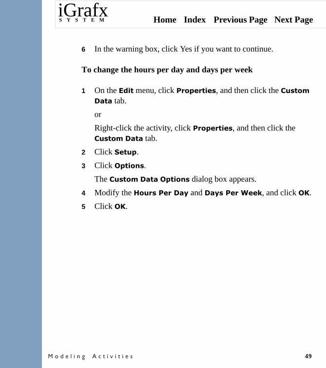
6 In the warning box, click Yes if you want to continue.
To change the hours per day and days per week
1 On the +��� menu, click ����������, and then click the �����! ���� tab.
or
Right-click the activity, click ����������, and then click the �����! ���� tab.
2 Click �����.
3 Click ������.
The �����! ���� ������ dialog box appears.
4 Modify the ,�����������$ and ��$������%���, and click ��.
5 Click ��.

Home Index Previous Page Next PageiGrafxS Y S T E M
� � � � � � � � � � � � � � � � � � � � � � � � � � 50
Editing Using the Tabular View
Using the Tabular View
Process diagrams can be viewed using the normal (graphical) view or the tabular view. Both views contain the same data and can be used to define a process diagram. Use the tabular view for the following:
• If you prefer entering or editing data using tables instead of graphics.
• If you have a large amount of data to enter.
About Tables in the Tabular View
Select the Tabular command on the View menu to change the view of the active process diagram from normal to tabular. The tabular view consists of a process table that contains the process diagram data. A unique cell name (row name) is assigned for each department and activity (for example, A1and B1) in the table. Connections to other symbols appear in the last column of the table as references to other cell names (A1 to B3).
A monitor appears in the tabular view as a small clock character to the left of the cell name. A start point appears as rounded rectangle inside the cell name.

Home Index Previous Page Next PageiGrafxS Y S T E M
� � � � � � � � � � � � � � � � � � � � � � � � � � 51
To switch to normal (graphical) view
On the (�� menu, click &��!� .
The process diagram is represented by symbols and directed lines.
To switch to tabular view
On the (�� menu, click ��#� ��.
The process diagram is represented in a process table.
To edit process data using the tabular view
1 Open an existing process diagram.
2 On the (�� menu, click ��#� ��.
The process diagram is represented in a process table.
Using the Tabular View to Add Data to a Process Diagram
You can create a process diagram by entering all the data in the tabular view. You can switch back and forth between the tabular and normal (graphical) views using the Normal and Tabular commands on the View menu.
Home Index Previous Page Next PageiGrafxS Y S T E M
� � � � � � � � � � � � � � � � � � � � � � � � � � 52
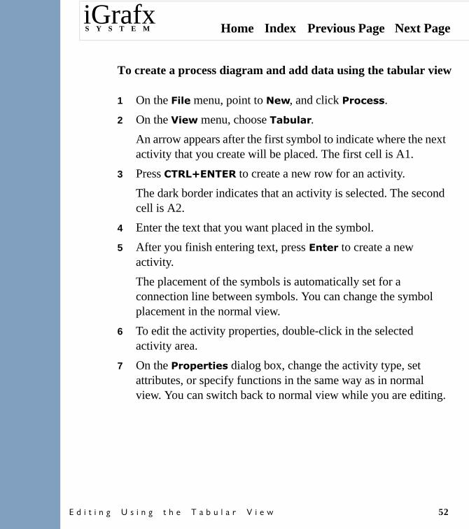
To create a process diagram and add data using the tabular view
1 On the �� � menu, point to &� , and click�������.
2 On the (�� menu, choose ��#� ��.
An arrow appears after the first symbol to indicate where the next activity that you create will be placed. The first cell is A1.
3 Press ���./+&�+� to create a new row for an activity.
The dark border indicates that an activity is selected. The second cell is A2.
4 Enter the text that you want placed in the symbol.
5 After you finish entering text, press +��� to create a new activity.
The placement of the symbols is automatically set for a connection line between symbols. You can change the symbol placement in the normal view.
6 To edit the activity properties, double-click in the selected activity area.
7 On the ���������� dialog box, change the activity type, set attributes, or specify functions in the same way as in normal view. You can switch back to normal view while you are editing.

Home Index Previous Page Next PageiGrafxS Y S T E M
� � � � � � � � � � � � � � � � � � � � � � � � � � 53
Connecting Symbols in Tables
You can connect symbols in a table by using the mouse to choose the source and destination symbols. The appropriate attachment point is automatically selected.
To connect symbols (activities) using the tabular view
1 On the (�� menu, click ��#� ��.
2 Cancel the selection of any cells.
Place the arrow cursor in the source symbol.
3 Press and drag the mouse button to the destination symbol.
4 Release the mouse button.
The connection remains selected until you perform an action such as pressing +��� to create another activity. The attachment point and the symbol placement are automatic.

Home Index Previous Page Next PageiGrafxS Y S T E M
� � � � � � � � � � � � � � � � � � � � � � � � � � 54
To delete a connection
1 On the (�� menu, click ��#� ��.
2 Click the connection that you want to delete.
3 On the +��� menu, click �� ���.
or
Press the �� ��� key.
To move a connection
To move a connection line, delete the old connection and create a new one.
Viewing Columns in Tabular View
The information is stored in columns sorted by modeling topics such as inputs, outputs, and so on. Each topic can have multiple columns (for example, the Task topic display has nine columns of data). You can choose which topics to display using the Columns command on the View menu. This makes it easier to find the information that you need.

Home Index Previous Page Next PageiGrafxS Y S T E M
� � � � � � � � � � � � � � � � � � � � � � � � � � 55
To choose which columns to display in the tabular view
1 On the (�� menu, choose �� �!�.
The ��� 0,������ �!� dialog box appears.
NoteThe Columns command is not available unless you are in Tabular view.
2 Select the columns of tabular information that you want to view.
Changing Styles in Tables
Most menus are available in either normal or tabular view, and the method for editing is usually the same after items are selected.
To change the font, fill, or border in the tabular view
To change the fill or border, select the cell area, click the right mouse button, and click ���!��.
To change the font, select the cell area, click the right mouse button, and click ���.
To change the line or arrow in the tabular view
Select the connection area., click the right mouse button, and click ���!��.
Home Index Previous Page Next PageiGrafxS Y S T E M
� � � � � � � � � � � � � � � � � � � � � � � � � � 56
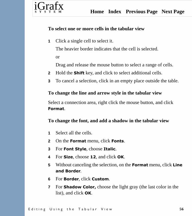
To select one or more cells in the tabular view
1 Click a single cell to select it.
The heavier border indicates that the cell is selected.
or
Drag and release the mouse button to select a range of cells.
2 Hold the ����� key, and click to select additional cells.
3 To cancel a selection, click in an empty place outside the table.
To change the line and arrow style in the tabular view
Select a connection area, right click the mouse button, and click ���!��.
To change the font, and add a shadow in the tabular view
1 Select all the cells.
2 On the ���!�� menu, click ����.
3 For ������$ �, choose �� ��.
4 For ��1�, choose 23, and click ��.
5 Without canceling the selection, on the ���!�� menu, click .������������.
6 For ������, click �����!.
7 For ����� ��� ��4 choose the light gray (the last color in the list), and click ��.

Home Index Previous Page Next PageiGrafxS Y S T E M
� � � � � � � � � � � � � � � � � � � � � � � � � � 57
8 ���� the selection by clicking outside the table.
The text is in an italic font face and the symbols have a gray shadow.
Moving, Copying, and Deleting Cells
After you create a cell, you can move it by selecting it, and then cutting and pasting it using the Clipboard. Connections between symbols that are moved using the Clipboard have to be redrawn after the symbol is moved.
To move one or more cells in the tabular view
1 Select the cell(s).
Selected cells have a heavier or highlighted border.
2 On the +��� menu, choose ���.
3 Move the cursor to the cell directly above the new location and click.
4 On the +��� menu, choose �����.
The cells are renumbered.
5 Create a new connection for the pasted cell.

Home Index Previous Page Next PageiGrafxS Y S T E M
� � � � � � � � � � � � � � � � � � � � � � � � � � 58
To copy and paste a cell in the tabular view
1 Select the cell.
2 On the +��� menu, choose ���$.
3 Move the cursor to the cell above the new location and click the cursor.
4 On the +��� menu, choose �����.
To cut or delete cells in the tabular view
1 Select one or more cells.
2 On the +��� menu, click ��� or �� ���
or
Press �� ���.

Home Index Previous Page Next PageiGrafxS Y S T E M
� � � � � � � � � � � � � � � � � � � � � � 59
Describing Model Behavior
Describing Model Behavior Using the Model Commands
Use the commands on the Model menu and the Model toolbar to add attributes, expressions, schedules, events, and functions to your model to analyze process inputs, outputs, and events.
TipThe commands on the Model menu are also found on the Model toolbar. On the View menu, click Toolbars to display the Toolbars dialog box. Use this dialog box to display the Model toolbar, to add, and to remove tools from the toolbar.
About Transaction Attributes
Transactions are the tokens that flow through a process. A transaction attribute is a variable that can have a unique value for each transaction. Each transaction can have its own set of attribute values that describe the transaction.

Home Index Previous Page Next PageiGrafxS Y S T E M
� � � � � � � � � � � � � � � � � � � � � � 60
Transaction attribute values are similar to cells in a spreadsheet or a table column. For example, the Priority attribute, a predefined (default) attribute, can have a different value at each transaction (Priority=3 for the first transaction, Priority=1 for the second transaction, and Priority=4 for the third transaction).
Common Uses for Transaction Attributes
Transaction attributes have the following common uses:
• Setting the duration of an activity based on the specifics of a transaction. For example, an activity duration is measured in seconds and uses an expression that contains the attribute PageCount multiplied by 5 (if PageCount is 100, then the duration is 500 seconds).
• Controlling the flow of specific transactions through a decision output.
• For example, as each transaction is processed by the activity, the value of Color determines whether the transaction takes the Blue, Red, or Yellow path.

Home Index Previous Page Next PageiGrafxS Y S T E M
� � � � � � � � � � � � � � � � � � � � � � 61
Defining a Transaction Attribute
When you define a transaction attribute, you specify its name, location, and type. For example, you can create and define transaction attributes for Color and PageCount. You can set the value for an attribute for each transaction.
To define a transaction attribute
1 On the ���� menu, click �����#����.
or
On the ���� toolbar, click the �����#���� tool.
The �����������#���� dialog box appears, and displays a list of existing attributes sorted by .������.
2 To view the attributes for another location, select another location.
Priority
Page Count
Color
Transaction Attributes
Value for first transaction
Value for second
transaction
Value for third transaction
3 1 4Pre-definedattribute
User-definedattribute

Home Index Previous Page Next PageiGrafxS Y S T E M
� � � � � � � � � � � � � � � � � � � � � � 62
The attributes for the selected location appear in the dialog box.
3 To add an attribute, click ���.
The�����&� ������#��� dialog box appears.
4 To modify an attribute, click �����$.
The �����$������#��� dialog box appears.
NoteYou can change only the attribute type or definition.
5 Use this dialog box to define the attribute name, type, location, initial values, and associate the attribute type departments, and processes.
6 To add or modify an attribute type, click �������$���.
The��������$��� dialog box appears.
7 Type the attribute �$���&�!�, and type the ��!#���, and click ��� or �����$.
The new or modified attribute type appears in the +*����- list.
8 Click �� to return to the ����&� ������#��� dialog box.
9 Click �� to return to the �����������#���� dialog box.
10 Click ��.

Home Index Previous Page Next PageiGrafxS Y S T E M
� � � � � � � � � � � � � � � � � � � � � � 63
Setting a Value When the Transaction Is Created
You can initialize the value of a transaction attribute when the transaction is created or at individual activities as transactions flow through the process. For example, after you define transaction attributes named Color, PageCount, and Fruit, their values can be initialized.
A generator is typically used to initialize transaction attributes. When you set the scenario data for simulation, you define the generator. By default, the value of an attribute is initialized to be its first member. If the value is defined as number type, the default initial value is 0.
Initializing a Transaction Attribute
There are two common methods of initializing a transaction attribute:
• By distribution• Using constant value and multiple generators
To initialize a transaction attribute by distribution
For example, you can use a generator to set an initial value based on a range of values.
1 On the ���� menu, click �����#����.
or
On the ���� toolbar, click the �����#���� tool.

Home Index Previous Page Next PageiGrafxS Y S T E M
� � � � � � � � � � � � � � � � � � � � � � 64
The �����������#���� dialog box appears and displays a list of existing attributes sorted by .������.
2 Use this dialog box to add the transaction attribute ����� and the type name ���������.
3 Add the following members to ���������: ��� �, ����, and ���-�.
4 On the ���� menu, click �������.
or
On the ���� toolbar, click the ������� tool.
5 Define the function �����������#����. This function is the same type, ���������, as the ����� attribute. Thirty percent of the time that �����������#���� is called, ��� � is returned; forty-five percent of the time, ����; and twenty-five percent, ���-�.
6 On the ���� menu, click ���������.
or
On the Model toolbar, click the ��������� tool.
7 Define a generator to initialize ����� with a value returned by �����������#����.

Home Index Previous Page Next PageiGrafxS Y S T E M
� � � � � � � � � � � � � � � � � � � � � � 65
To initialize a transaction attribute by constant value and multiple generators
1 On the ���� menu, click ���������.
or
On the ���� toolbar, click the ��������� tool.
The ��������������� dialog box appears.
2 Use this dialog box to define ���������.
You can use a constant to set the same value for any transaction created by a generator by defining a separate generator to initialize different values for the transaction attribute.
For example, one generator issues transactions in which ����� is set to ��� �, a second generator sets ����� to ����, and the third generator sets ����� to ���-�.
Setting a Value in the Process Flow
The value of a transaction attribute can be set or changed on an activity. This method works particularly well if there is a decision in the process flow that identifies specific transactions. Every transaction that reaches the activity is assigned the attribute values.
The Attributes tab on the Properties Dialog box defines the value of attributes for any specific activity.

Home Index Previous Page Next PageiGrafxS Y S T E M
� � � � � � � � � � � � � � � � � � � � � � 66
Using Monitors and Transaction Attributes
You can place monitors to track statistics based on transaction attributes. This is useful for looking at cycle time, waiting time, or any transaction statistics for specific transactions.
Setting a Priority on a Transaction
You can use the Priority transaction attribute to specify the order in which transactions are transacted. When transactions are queued (for example, waiting for a worker or at a batch activity), the highest priority transactions are always transacted first.
• A higher priority transaction is processed before all lower priority transactions that are waiting.
• Two transactions with the same level of priority are processed in the order that they arrive.
• A higher priority transaction never acquires resources away from transactions that are already in process unless preempt is set.
The Priority transaction attribute is a predefined attribute for all activities and generators. You can set the following values for the Preempt transaction attribute:
• Constant. The value can be between 0 and 127 where 0 is the lowest priority. By default, transactions have a priority of 0.
• Expression. You can define the priority value with an expression that uses different attributes, functions, and arithmetic operators.
Home Index Previous Page Next PageiGrafxS Y S T E M
� � � � � � � � � � � � � � � � � � � � � � 67
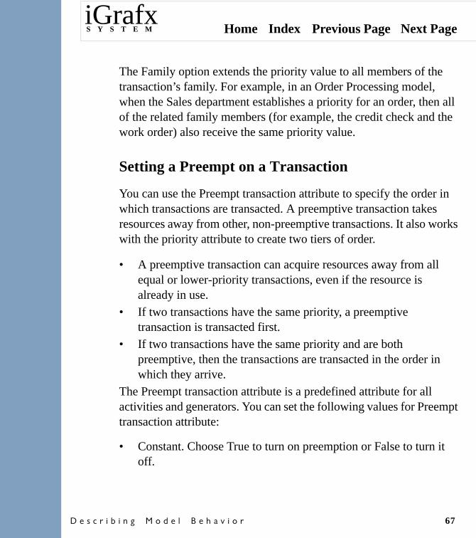
The Family option extends the priority value to all members of the transaction’s family. For example, in an Order Processing model, when the Sales department establishes a priority for an order, then all of the related family members (for example, the credit check and the work order) also receive the same priority value.
Setting a Preempt on a Transaction
You can use the Preempt transaction attribute to specify the order in which transactions are transacted. A preemptive transaction takes resources away from other, non-preemptive transactions. It also works with the priority attribute to create two tiers of order.
• A preemptive transaction can acquire resources away from all equal or lower-priority transactions, even if the resource is already in use.
• If two transactions have the same priority, a preemptive transaction is transacted first.
• If two transactions have the same priority and are both preemptive, then the transactions are transacted in the order in which they arrive.
The Preempt transaction attribute is a predefined attribute for all activities and generators. You can set the following values for Preempt transaction attribute:
• Constant. Choose True to turn on preemption or False to turn it off.

Home Index Previous Page Next PageiGrafxS Y S T E M
� � � � � � � � � � � � � � � � � � � � � � 68
• Expression. You can define the preemption value with an expression that uses different attributes, functions, and arithmetic operators.
Using Global Attributes
The three global attributes are department, process, and scenario. These attributes are considered separately from transaction attributes because of their different purposes. A transaction attribute provides individual values for transactions; a global attribute sets a value that all transactions can access.
• Scenario attributes have one global value at any time. This is the most commonly used global attribute.
• Department attributes have separate values for each defined department. A department can exist in multiple processes.

Home Index Previous Page Next PageiGrafxS Y S T E M
� � � � � � � � � � � � � � � � � � � � � � 69
• Process attributes have unique or separate values for each process.
To find the location of an attribute
1 On the ���� menu, click �����#����.
or
On the ���� toolbar, click the �����#���� tool.
2 In the������������#���� dialog box, click the .������ designation that you want for the attribute.
The dialog box displays the attributes sorted by location. The active location is indicated by the shaded button.
Department 1
Department 2
Process 1
Department 3
Department 1
Process 2
Department 1
Process 3
Department 4
Process Scenario attributes have one global value
Process attributes haveseparate values for different processes
Department attributeshave separate values for different departments

Home Index Previous Page Next PageiGrafxS Y S T E M
� � � � � � � � � � � � � � � � � � � � � � 70
Using Global Scenario Attributes
Scenario attributes are available to all activities. If a model has two scenarios, then the attribute values in Scenario1 are not available to activities in Scenario2. The scenario attribute prefix is S.
For example, a Review Committee keeps track of the number of times that a document is reviewed during its entire revision cycle. This uses a scenario attribute called ReviewCount. Any activity that reviews the document increments the count by 1.
Using Global Process Attributes
The value of a process attribute is available to activities in the process. The process encompasses the model and its activities. Activities in Process1, for example, can check or set process attribute values only in Process1. The process attribute prefix is P.
Using Global Department Attributes
Department attributes are available to any activity in the same department, regardless of process.
For example, each department in a Tax Office has its own tax rate. The fixed cost for an activity is multiplied by the specific department’s tax rate. A department attribute, Tax, is defined, with a different initial value for each department.

Home Index Previous Page Next PageiGrafxS Y S T E M
� � � � � � � � � � � � � � � � � � � � � � 71
The individual activities use Tax as a multiplier for the fixed cost. For example, the following activity has a fixed cost of 25 multiplied by the department’s tax rate. In other words, if this activity is in Dept. 3, the fixed cost is 72.5. If the activity is in Dept. 2, it is 70.
Setting Global Attribute Values
You can set the initial value for a global attribute as part of the simulation data.
To set global attribute values
1 On the ���� menu, click Attributes.
or
On the ���� toolbar, click the �����#���� tool.
The �����������#���� dialog box appears.
For example, a scenario attribute called ��! is initialized to 5. The � prefix indicates that the attribute has a scenario location.
2 Select a location (�������, �������, or ������!��).
3 Add or modify an existing attribute.
4 For ���� �(� ��, choose how the value is expressed and the value.
������—Insert or choose a value from the list. The value must be of the defined type for the attribute. For example, if the type is &�!#��, you can enter only a number.

Home Index Previous Page Next PageiGrafxS Y S T E M
� � � � � � � � � � � � � � � � � � � � � � 72
+*�������—Create the expression using attributes, functions, and arithmetic operators.
About Transactions and Report Results
Report statistics contain information gathered about global transactions.
Using Attribute Prefixes
An attribute prefix is assigned to all attributes that are not located at the transaction level to indicate their location. After you define an attribute, this prefix appears in the Attribute Settings list. You must enter the prefix when using the attribute name in an expression.
Type of attribute Prefix
Transaction attribute No prefix (for example attribute_name)
Process attribute P. (for example P.attribute_name)
Scenario attribute S. (for example S.attribute_name)
Department attribute D. (for example D.attribute_name)

Home Index Previous Page Next PageiGrafxS Y S T E M
� � � � � � � � � � � � � � � � � � � � � � 73
The prefix F. (for example F.attribute_name) assigns a value to a transaction attribute for each of the individual members of the transaction’s family. A transaction family is created the first time a transaction is split. For example, a transaction attribute is assigned a value with the expression: F.layer = 3. This assigns 3 to layer for all other transactions that are family members of the transaction that has the assignment.
Defining Attribute and Function Types
The type for an attribute or function defines its range of values. The default types are Number, YesNo, and TrueFalse. You can create your own type and specify the range for the type by adding members to the type. For example, create the type Reports, and assign the members Daily, Weekly, Monthly, EndOfYear.
• Number type sets the attribute value to any real number (to fifteen-digit precision).
• A YesNo type has a value of either No (equal to 0) or Yes (1).• A TrueFalse type specifies that the attribute can either have a
value of False (equal to 0) or True (1).Types are also used to create Decision paths and as case text labels.
To define an attribute type
1 On the ���� menu, click �$���.
2 In the��������$��� dialog box, type a name for the type.

Home Index Previous Page Next PageiGrafxS Y S T E M
� � � � � � � � � � � � � � � � � � � � � � 74
The name must have fewer than 32 characters and contain only alphanumeric characters. The name can contain the underscore character but no spaces. Types are case-sensitive.
3 Move the cursor into the ��!#��� box and click.
4 Type each of the members, pressing +��� to start a new line.
For example, define the type �� �� with members 5� � and ���.
5 To define another type, click ���.
Using Expressions
When a count or simple number is used in a model (for example, to set the duration for an activity or the length of time for simulation), you can substitute an expression or choose from the library of system functions.
An expression is a mathematical statement that equals a value or distribution. The values that you can set for modeling include simple and complex expressions.
Expressions can combine functions, attributes, numbers, and members with different mathematical operators, as shown in the following illustration.

Home Index Previous Page Next PageiGrafxS Y S T E M
� � � � � � � � � � � � � � � � � � � � � � 75
For example, on a Test activity, the first time a printed circuit board is tested, the test duration is 15 minutes. All subsequent tests take 25 minutes. The expression uses a function called If. The first argument of the function is an attribute, First_Time. For example, If(First_Time = True, 15, 25).
The advantage to using either the Expression builder or the Expression toolbar to create an expression is that you can often avoid common syntax errors.
E x p r e ssi o n s
M e m b e r s
N u m b e r s
A tt r i b u te s
F u n c t i o n s
T y p e s
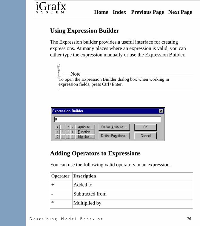
Home Index Previous Page Next PageiGrafxS Y S T E M
� � � � � � � � � � � � � � � � � � � � � � 76
Using Expression Builder
The Expression builder provides a useful interface for creating expressions. At many places where an expression is valid, you can either type the expression manually or use the Expression Builder.
NoteTo open the Expression Builder dialog box when working in expression fields, press Ctrl+Enter.
Adding Operators to Expressions
You can use the following valid operators in an expression.
Operator Description
+ Added to
- Subtracted from
* Multiplied by

Home Index Previous Page Next PageiGrafxS Y S T E M
� � � � � � � � � � � � � � � � � � � � � � 77
Expressions are evaluated according to the operators used and the placement of parentheses. The operations are performed from left to right in the following order.
/ Divided by
= Equal to
! Not (logical negation)
< Less than
> Greater than
<= Less than or equal to
>= Greater than or equal to
& Logical and Both statements must be true to return True.
| Logical or. Either statement can be true to return True.
( ) Parentheses
% Mod operator. Returns a remainder after a number is divided by a divisor.
, Comma. Used to separate members of a list of arguments.
Operator Description
( ) Parentheses
* / Multiplication and division
+ - Addition and subtraction

Home Index Previous Page Next PageiGrafxS Y S T E M
� � � � � � � � � � � � � � � � � � � � � � 78
To add attributes to expressions
If you know the name of the attribute, you can type it in as the expression. Otherwise, follow these steps to choose from the list of defined attributes.
1 On the +*������� toolbar or builder, click �����������#���.
The �����������#��� dialog box appears.
2 Select the attribute location.
Only attributes that have been defined for the selected location appear in the scrolling list.
3 Double-click the attribute that you want to paste.
4 When you finish using the �����������#���� dialog box, click ��.
The attribute is pasted into the expression.
NoteAttribute names are case sensitive. If you type an attribute into an expression, use the correct lowercase and uppercase characters.
< > <= >= != Comparisons
& and | Logical and and or

Home Index Previous Page Next PageiGrafxS Y S T E M
� � � � � � � � � � � � � � � � � � � � � � 79
To add members to expressions
If you know the name of the member, for example, True or False, you can type it into the expression. Otherwise, follow these steps to choose from the list of valid members.
1 On the +*������� toolbar or builder, click the���������!#�� tool.
2 In the ��������!#�� dialog box, click the type.
3 Double-click the member.
The function is pasted into the expression.
Using Functions
Although you can often use a simple number or a distributed value for things such as durations, you use a function for a non-constant value or a range of numbers. Functions are also convenient for creating a single place to change a value used in multiple places.
A function is a mathematical correspondence that returns a value for every value passed to it or generated by the system. You cannot edit the system-defined functions but you can create new functions.

Home Index Previous Page Next PageiGrafxS Y S T E M
� � � � � � � � � � � � � � � � � � � � � � 80
A function has one or more arguments. For example, the Between function returns a value that is uniform in the range between a minimum and maximum value. It has two arguments: min and max. You insert a minimum value, which is the lowest value that the function returns, and a maximum value, which is the highest. In the following expression, the duration of an activity is a uniform number between 5 and 15.
For example, Between(5,15).
Other system-defined functions map a number to a unit of time. For example, the following expression returns a value of 2, because there are 7200 seconds in two hours.
For example, Hours(7200).
Using System-Defined Functions
The graphs for the probability distribution functions in this section were created by running 5,000 transactions through a single activity whose duration was defined to be the specific distribution function. All 5,000 transactions were generated at the start of simulation.
All simulations were run for 200 seconds and snapshots were taken every 10 seconds. The number of transactions completed during each snapshot time was graphed versus the time of the snapshot.

Home Index Previous Page Next PageiGrafxS Y S T E M
� � � � � � � � � � � � � � � � � � � � � � 81
The graphs are not smooth curves because the amount of transactions is sampled every ten seconds. Also, not enough transactions are run to completely smooth out the effects of randomness from the random number generator.
List of System-Defined Functions
Function Description
Abs(n) This returns the absolute value of a number. The absolute value is the number without a sign. For example: Abs(-4) = 4, Abs(9) = 9
BernoulliDist(Probability) The Bernoulli distribution returns a value of 1 or 0; the argument indicates how frequently the value of 1 is returned on a percentage basis. For example: BernoulliDist(0.7) implies a value of 1 is returned 70% of the time
BetaDist(A,B,Min, Max) This returns the cumulative Beta probability density function between the minimum and maximum values that you supply. The BetaDist function is commonly used to study variation in a percentage across samples.
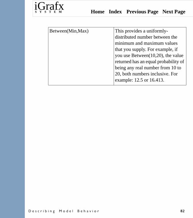
Home Index Previous Page Next PageiGrafxS Y S T E M
� � � � � � � � � � � � � � � � � � � � � � 82
Between(Min,Max) This provides a uniformly-distributed number between the minimum and maximum values that you supply. For example, if you use Between(10,20), the value returned has an equal probability of being any real number from 10 to 20, both numbers inclusive. For example: 12.5 or 16.413.

Home Index Previous Page Next PageiGrafxS Y S T E M
� � � � � � � � � � � � � � � � � � � � � � 83
BetweenNorm(Min,Max) This provides a Normal random variable between a minimum and maximum value. For example, if you use BetweenNorm(10,20), the value returned is more likely to be 14, 15, or 16, and seldom 10 or 20. The following graph shows three simulations of a single activity whose duration is specified as a BetweenNorm distribution.
This function is the same as the NormDist function except that the mean and standard deviation are calculated automatically according to the minimum and maximum values that you provide. Also, the value returned will always be inside the specified range.
BinomDist(N,Probability) The Binomial distribution models drawing or selecting items from a pool, where N is the number of items in the pool and Probability is the probability of each item being successfully drawn.

Home Index Previous Page Next PageiGrafxS Y S T E M
� � � � � � � � � � � � � � � � � � � � � � 84
Ceiling(Num) This returns a number rounded up to a whole number. The number can be zero or negative. For example: Ceiling(2.5) = 3, Ceiling(0) = 0, Ceiling(-4.37) = -4.

Home Index Previous Page Next PageiGrafxS Y S T E M
� � � � � � � � � � � � � � � � � � � � � � 85
Cost(Value,Labor/Equipment/Other, Standard/Overtime)
This returns the costs accumulated on a transaction in the different cost categories. The cost is calculated up to the point in time in the simulation when the function is called. A value of zero returns all cost categories.
Value1 = Value Added2 = Business Value Added3 = Value Added + Business Value Added4 = No Value Added5 = Value Added + No Value Added6 = Business Value Added + No Value Added7 = Value Added + Business Value Added + No Value Added
Labor/Equipment/Other1 = Labor2 = Equipment3 = Labor +Equipment4 = Other5 = Labor + Other6 = Equipment + Other7 = Labor + Equipment + Other

Home Index Previous Page Next PageiGrafxS Y S T E M
� � � � � � � � � � � � � � � � � � � � � � 86
Standard/Overtime1= Standard cost (non-overtime)2 = Overtime3 = Standard + Overtime (same as using 0)
Days(Seconds) This converts the argument from seconds to days. The Days function uses the run setup information to calculate how many hours are in a day. For example, if there are 8 hours in a day, then Days(201600) = 7.
DaysToSec(Days) This converts the argument from days to seconds. This is the inverse function for Days().
ElapsedTime () This returns the amount of time that has elapsed since the start of the simulation, in seconds. For example, ElapsedTime() after four hours of simulation = 14400.

Home Index Previous Page Next PageiGrafxS Y S T E M
� � � � � � � � � � � � � � � � � � � � � � 87
ErlangDist(N,B) The Erlang distribution generates random values where N is the mean distribution and B is the variance. Both N and B must be greater than zero and N is an integer. (The Erlang distribution is a subset of the Gamma distribution.)
Exp(Num) This returns e raised to the power of Num. The constant e equals 2.71828182845904, the base of the natural logarithm. For example: Exp(1) = 2.71828.
ExponDist(Mean) This provides an exponential random variable. The variable is described completely by specifying a single property, the mean. For example, if you specify ExponDist(15), the resulting value, over time, will be close to 15. Spikes of much larger or smaller numbers are always possible with the exponential distribution.
aN xN-1 e-bx
(N-1)!

Home Index Previous Page Next PageiGrafxS Y S T E M
� � � � � � � � � � � � � � � � � � � � � � 88
Floor(Num) This rounds a number down to a whole number. For example: Floor(4.3) = 4, Floor(.119) = 0, Floor(-5.4) = -6.
GammaDist(A,B) The Gamma distribution generates random values with the following density:
Hours(Seconds) This converts the argument from seconds to hours by dividing by 3600. For example: Hours(32400) = 9.
HoursToSec(Hours) This converts the argument from hours to seconds. This is the inverse function for Hours().
AB
Gamma(B) xB-1 e-

Home Index Previous Page Next PageiGrafxS Y S T E M
� � � � � � � � � � � � � � � � � � � � � � 89
If(Test,True,False) This provides an If function that checks the condition of Test. If Test is true, the value returned is set by the variable labeled True. If Test is false, the value is set by the variable labeled False. The True and False arguments can be expressions themselves. For example, if you have an attribute named Apple whose value is Red, then the following expression returns 5. If the value of Apple is Green, the expression returns 10. For example: If(Apple=Red,5,10). If Apple is Red, then the following expression returns 5. If Apple is Green, the expression returns 10. If Apple is not Red or Green, the expression returns 15. For Example: f(Apple=Red,5,(If(Apple=Green,10,15))).

Home Index Previous Page Next PageiGrafxS Y S T E M
� � � � � � � � � � � � � � � � � � � � � � 90
Ln(Num) This returns the natural logarithm (the inverse of the Exp function). The number must be positive. For example, Ln(55) = 4.00733, Ln(Exp(4)) = 4, Ln(2.71828) = .9999.
Log10(Num) This returns the base 10 logarithm of a number. The number must be positive. For example, Log10(5) = .69897.
LogNormDist(Mean,Deviation) This is the logarithmic normal distribution. The first parameter is the mean and the second is the deviation.
Max(Num,Num) This returns the largest number of the two arguments. For example, Max(4,9) = 9.
Min(Num,Num) This returns the smallest number of the two arguments. For example, Max(4,9) = 4.
Minutes(Seconds) This converts the argument from seconds to minutes. For example, Minutes(4500) = 75.
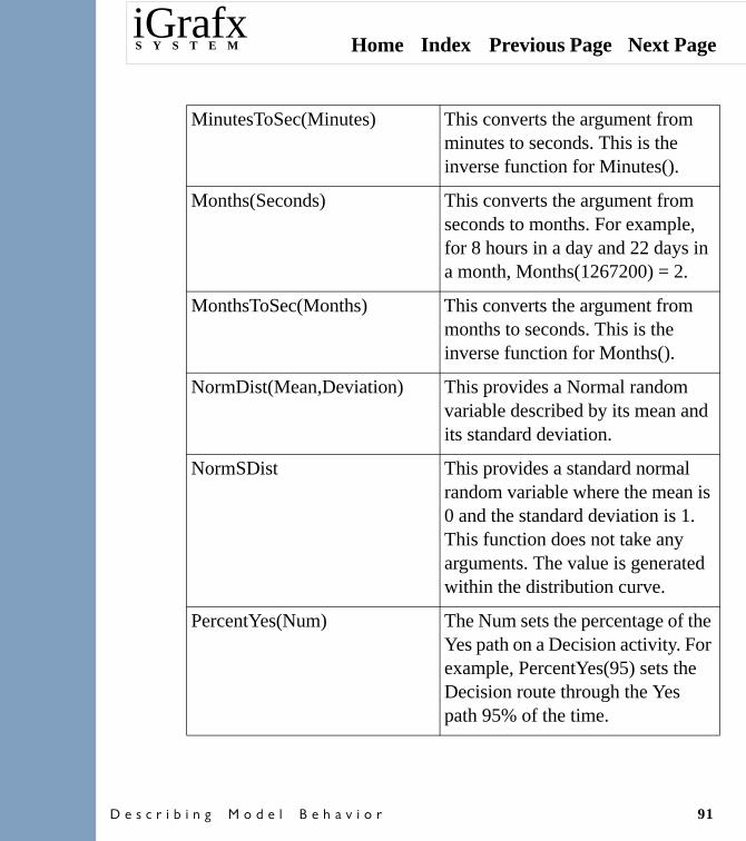
Home Index Previous Page Next PageiGrafxS Y S T E M
� � � � � � � � � � � � � � � � � � � � � � 91
MinutesToSec(Minutes) This converts the argument from minutes to seconds. This is the inverse function for Minutes().
Months(Seconds) This converts the argument from seconds to months. For example, for 8 hours in a day and 22 days in a month, Months(1267200) = 2.
MonthsToSec(Months) This converts the argument from months to seconds. This is the inverse function for Months().
NormDist(Mean,Deviation) This provides a Normal random variable described by its mean and its standard deviation.
NormSDist This provides a standard normal random variable where the mean is 0 and the standard deviation is 1. This function does not take any arguments. The value is generated within the distribution curve.
PercentYes(Num) The Num sets the percentage of the Yes path on a Decision activity. For example, PercentYes(95) sets the Decision route through the Yes path 95% of the time.

Home Index Previous Page Next PageiGrafxS Y S T E M
� � � � � � � � � � � � � � � � � � � � � � 92
PoissonDist(Mean) The Poisson distribution is a limiting form of the Binomial distribution when, in the Binomial expression, N tends to infinity and Probability tends to zero at the same time. Exponential interarrivals are the same as Poisson arrivals.
Power(Num,Exp) This returns Num to the power of Exp. For example, Power(5,3) = 125, Power(1,5) = 1, Power(10,5) = 100000.
Random() Provides a standard normal random variable between 0 and 1.
e-Mean Meanx
x!

Home Index Previous Page Next PageiGrafxS Y S T E M
� � � � � � � � � � � � � � � � � � � � � � 93
Round(Num,Numdigits) This rounds the number to the number of specified digits. If NumDigits is greater than zero, it rounds to the specified decimal places. If NumDigits equals zero, it rounds to the nearest integer. If NumDigits is less than zero, it rounds to the left of the decimal. For example, Round(3.45, 1) = 3.5, Round(11.5,-1) = 10.
Sqrt(Num) This returns the positive square root. The number must be positive. For example, Sqrt(25) =5.
Time(Timetype) This returns the amount of time that has accumulated on a transaction, in different categories, since the start of the simulation. The time is given in seconds with 0 = Cycle time,1 = Work time, 2 = Resource waiting time, 3 = Blocked time, and 4 = Inactive time. For example, if ten minutes of inactive time has accumulated, Time(4) returns 600.

Home Index Previous Page Next PageiGrafxS Y S T E M
� � � � � � � � � � � � � � � � � � � � � � 94
TransServiceTime() This returns the accumulated service time of a transaction up until the point that the function is evaluated. This does not include the duration on the current activity if it is evaluated as Attribute Settings Before Duration.
TransWaitingTime() This returns the accumulated waiting time of a transaction up until the point that the function is evaluated. This does not include the duration on the current activity if it is evaluated as Attribute Settings Before Duration.
TriangleDistribution(Min,Max,Mean)
This returns the value of a Triangle distribution.
Trunc(Num,Numdigits) This rounds the number toward zero to the nearest integer or nearest NumDigits decimal place. For example: Trunc(9.765,0) = 9, Trunc(9.765,2) = 9.76, Trunc(65, -1) = 60, Trunc (-9.765, 2) = -9.76.

Home Index Previous Page Next PageiGrafxS Y S T E M
� � � � � � � � � � � � � � � � � � � � � � 95
Weeks(Seconds) This converts the argument from seconds to weeks. The function uses the run setup information to calculate how many days are in a week. For example, if there are 5 days in a week and 8 hours in a day, then Weeks(6480000) = 45.
WeeksToSec(Weeks) This converts the argument from weeks to seconds. This is the inverse function to Weeks().
WeibullDist(A,B) The Weibull distribution is typically used for reliability analysis. It takes two parameters, A and B. Both must be greater than 0. For example, We(x) = ABx(B-1) e-AxB
Years(Seconds) This converts the argument from seconds to years. The function uses the run setup to calculate the length of a year. For example, if there are 22 days in a month and 8 hours in a day, then Years(7603200) = 1.
YearsToSec(Years) This converts the argument from years to seconds. This is the inverse function to Years().
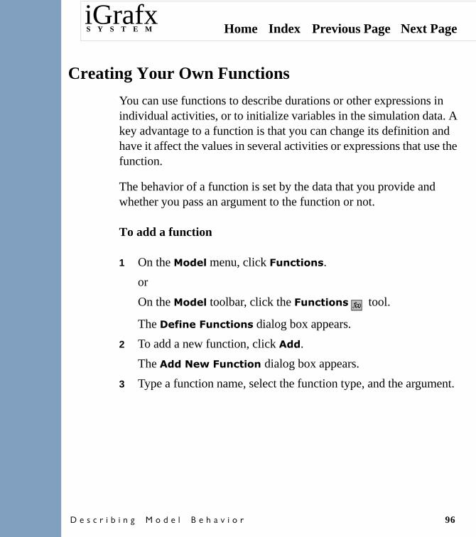
Home Index Previous Page Next PageiGrafxS Y S T E M
� � � � � � � � � � � � � � � � � � � � � � 96
Creating Your Own Functions
You can use functions to describe durations or other expressions in individual activities, or to initialize variables in the simulation data. A key advantage to a function is that you can change its definition and have it affect the values in several activities or expressions that use the function.
The behavior of a function is set by the data that you provide and whether you pass an argument to the function or not.
To add a function
1 On the ���� menu, click �������.
or
On the ���� toolbar, click the ������� tool.
The ������������� dialog box appears.
2 To add a new function, click ���.
The ����&� ��������dialog box appears.
3 Type a function name, select the function type, and the argument.

Home Index Previous Page Next PageiGrafxS Y S T E M
� � � � � � � � � � � � � � � � � � � � � � 97
To define a function
1 On the ���� menu, click �������.
or
On the ���� toolbar, click the ������� tool.
The�������������� dialog box appears. A list of existing functions is displayed and the current function is highlighted.
2 To define the values of a function, click the function name from the list of existing functions.

Home Index Previous Page Next PageiGrafxS Y S T E M
� � � � � � � � � � � � � � � � � � 98
Running a Simulation
Getting Started With Simulation
After you create the process diagram and model, you can simulate it. When a process is simulated, it runs through a processor that takes the information in the process diagram, including the activities and accompanying logic, and runs it for a set amount of time. This produces statistical results based on the model.
The process for setting up the simulation environment includes determining the duration of the simulation run, the schedule, the inputs, and the resource availability and requirements.
When setting up model data and running a simulation, you typically perform the preliminary steps to specify information about the simulation. After that, you may need to make few, if any, modifications to the settings as you run subsequent simulations.
Describing the iGrafx Process 2000 Simulation Methodology
The simulation method used by iGrafx Process 2000 is called discrete event simulation. In a discrete event system, the system changes from one distinct state to another as activities occur in a series of individual steps. This change in state can occur in any of the potentially thousands of variables in the model. For example, the number of transactions in a particular queue can decrease, or the status of a

Home Index Previous Page Next PageiGrafxS Y S T E M
� � � � � � � � � � � � � � � � � � 99
particular resource can change from busy to out of service. In other words, an iGrafx Process 2000 model changes state at discrete points in time as the result of simulation events.
A discrete system uses variables that can take on only particular values from among a finite (but potentially very large) set of alternatives. For example, the users of a telephone booth are engaged in a series of discrete activities. Customers arrive at the booth and wish to make a call. If the booth is busy, the caller creates or joins the waiting line. When the booth is available, the first person in line uses the phone for a certain amount of time. The person then leaves, making the booth available for the next caller.
At any time, the state of the telephone booth can be specified by a variable that indicates the activity in progress.

Home Index Previous Page Next PageiGrafxS Y S T E M
� � � � � � � � � � � � � � � � � � 100
About the iGrafx Process 2000 Environment
A scenario is a set of data about the simulation environment. It includes the run setup, generators, resources, schedule definitions, and other simulation options. A simulation run uses one or more process diagrams in association with a scenario. The combination of process diagrams and scenarios provides the environment within which to run a simulation.
You can have several scenarios in one file for running different variations. Also, a simulation can use activities from more than one process and the results from multiple reports can be compared side-by-side. The following illustration shows this relationship between multiple processes, scenarios, and reports. Each model file contains some or all of these elements.
To set up a simulation
1 On the ���� menu, click �������� to set the start and length of the simulation.
or
On the ���� toolbar, click the �������� tool.
2 On the ���� menu, click ��������� to set the rate at which transactions are introduced into the process.
3 Click ��������� to set the resources available to the process. For example, 3 workers and 1 machine.

Home Index Previous Page Next PageiGrafxS Y S T E M
� � � � � � � � � � � � � � � � � � 101
4 On the ���� menu, point to ��, and then click ����� to simulate the model
Setting Up a Simulation Run
Setting up a simulation run requires you to define scenario data. For example you define the type of simulation time used, when the simulation ends, and the time conversion units.
To set the simulation time
1 On the ���� toolbar, click the��������� tool.
or
On the ���� menu, click ��������.
2 In the �������� dialog box, click the ��!� �������!� tab.
3 Enter the simulation time parameters.

Home Index Previous Page Next PageiGrafxS Y S T E M
� � � � � � � � � � � � � � � � � � 102
To set the run initialization options (active limit and sequence)
1 On the ���� toolbar, click the �������� tool.
or
On the ���� menu, click �� �����.
2 In the �� ����� dialog box, click the����� �1����0������ tab.
3 Enter the run initialization options (for example, the active limit and the sequence).
4 Click another tab and enter additional data, or Click ��.
Taking Snapshots During a Simulation
A snapshot is a defined time when data accumulation occurs. By default, data is captured in the report at the end of simulation. Using snapshots enables you to capture data at other points during simulation.
To snapshot model data
1 On the ���� toolbar, click the �� ����� tool.
2 In the �� ����� dialog box, choose the �������� tab.
3 Add, modify, or delete a snapshot interval.

Home Index Previous Page Next PageiGrafxS Y S T E M
� � � � � � � � � � � � � � � � � � 103
Using Generators
A generator introduces transactions into the process at the first activity or at other entry points. It enables you to set a rate at which transactions enter the process. You can think of the generator as the driving force behind the process. For example, each generated transaction can represent a customer submitting an order or a new product being developed.
There are five types of generators. Depending on the type of generator you choose, the transactions enter one at a time, in multiples, or whenever a resource is available.
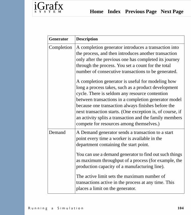
Home Index Previous Page Next PageiGrafxS Y S T E M
� � � � � � � � � � � � � � � � � � 104
Generator Description
Completion A completion generator introduces a transaction into the process, and then introduces another transaction only after the previous one has completed its journey through the process. You set a count for the total number of consecutive transactions to be generated.
A completion generator is useful for modeling how long a process takes, such as a product development cycle. There is seldom any resource contention between transactions in a completion generator model because one transaction always finishes before the next transaction starts. (One exception is, of course, if an activity splits a transaction and the family members compete for resources among themselves.)
Demand A Demand generator sends a transaction to a start point every time a worker is available in the department containing the start point.
You can use a demand generator to find out such things as maximum throughput of a process (for example, the production capacity of a manufacturing line).
The active limit sets the maximum number of transactions active in the process at any time. This places a limit on the generator.

Home Index Previous Page Next PageiGrafxS Y S T E M
� � � � � � � � � � � � � � � � � � 105
To define a generator
1 On the ���� toolbar, click the ��������� tool, and
double-click ��������2 in the generator window docked at the bottom of your screen.
The ����� ��������� dialog box appears.
For +*����-����������, click to select the generator name. To create a new generator, click ���. To delete a generator, select it and click �� ���.
Interarrival This generator issues transactions at a defined rate. You set the count and interarrival time. You can use this generator to model regular processes such as an order entry system where transactions occur on a regular basis.
Event This generator issues transactions at the occurrence of a specific time event (e.g., weekly, first of the month).
You can use this generator to simulate transactions that occur at a specific time such as first of the month bills.
Timetable This generator issues transactions based on a table that specifies the numbers of transactions to be issued in each specified time period.
You can use this table to define time periods (hours, days, months) and the number of transaction that are issued in each time period.

Home Index Previous Page Next PageiGrafxS Y S T E M
� � � � � � � � � � � � � � � � � � 106
Using Resources
The resource list describes the number of workers and other resources available to the model.
To define resources
1 On the ���� toolbar, click the �������� tool.
or
On the ���� menu, click ���������.
The ����� ��������� dialog box appears.
Under +*����-����������, the %����� resource is automatically defined for all models. This resource is automatically assigned a .�#�� resource type.
• To add a resource, click ���.
In the ����&� ��������� dialog box, type a new name under ���������&�!� and choose a ����������$��.
• To modify a resource, select its name from the +*����-�
��������� list and click �����$.
Home Index Previous Page Next PageiGrafxS Y S T E M
� � � � � � � � � � � � � � � � � � 107
About Resource Costs
Activities can accumulate costs during simulation to provide data about different expenses. You set the costs to accumulate in two different places.
• A cost can be part of an activity base that includes fixed and value cost.
• A cost can be set as a result of resources used. The resource cost for an activity is the combination of its resources’ hourly rate, per use cost, and overtime hourly rate.
Different units of time are converted automatically; for example, a rate can be in hours while the duration is days.
• Hourly Rate. The total hourly rate is calculated using the resource busy time.
• Per Use. This is a cost that accumulates each time the resource is used. For example, a duplicating machine accrues $.05 for every copy it makes.
• Hourly Rate (Overtime). The overtime rate is calculated when a resource enters overtime. Whether a resource uses overtime depends on the resource behavior, the activity behavior, and the resource’s schedule.
• Maximum Hours Per Day (Overtime). This sets the maximum overtime hours allowed for the resource on this activity. For example, a machine can run only two hours over its regular schedule.

Home Index Previous Page Next PageiGrafxS Y S T E M
� � � � � � � � � � � � � � � � � � 108
For example, workers are responsible for manufacturing plastic disks. The workers have a standard schedule, and are paid $12.00 an hour, $18 overtime, and are authorized to work up to one hour overtime a day. The workers use a plastic extruding machine that is always available. The machine costs $100 an hour to run, plus there is a per use cost of $75. For example, for two hours, assume one hour of regular time and one hour of overtime. One worker uses the machine. For the first hour, $12 of the worker’s hourly rate is accumulated, plus $100 for the machine’s hour and $75 per use. For the second hour, $18 of the worker’s overtime rate is accumulated, plus another $100 for the machine’s hour. The total for the two hours is $305.
Using Resource Pools
A pool is a group of identical resources. The resources in a pool are allocated and queued independently from other resources in other pools. You set the order that multiple pools are drawn from and the sequence for transactions to enter the queue. Each pool has its own allocation of resources.
iGrafx Process 2000 creates one pool for each department, even if the pool has only one worker. All other types of resources are combined into shared pools.

Home Index Previous Page Next PageiGrafxS Y S T E M
� � � � � � � � � � � � � � � � � � 109
To define resource pools
1 In the ��������������� dialog box, click ��"����.
The resources are arranged by pool.
2 (Optional) For ���������, click to select a pool.
Newly created pools are appended after the selected pool.
3 Click ������� .
A new pool is created. The pool name is dimmed if there are no departments assigned to it. The pool name is a series set by the system, for example, Pool-B, Pool-C, and so on.
The report area displays the pool information. For example, Dept. 1 uses Pool-A exclusively and Dept. 2 uses Pool-B exclusively. Pool-C has a single worker but is not assigned to any department.
4 When more than one process is open, you can share the resource pools between processes.
To separate the pools by process, select the �$���������check box.
To share the pools between processes, clear the �$�������� check box.

Home Index Previous Page Next PageiGrafxS Y S T E M
� � � � � � � � � � � � � � � � � � 110
Shared and Unshared Pools
A pool can be unshared or shared. In an unshared pool, resources are allocated to one department. In a shared pool, multiple departments and processes draw from the same pool when they acquire a resource.
You can view a diagram of shared pool allocations in the Scenario window under Resources.
To create shared or unshared resource pools
1 In the ��������������� dialog box, click ��"����.
The data in the dialog box is updated.
2 For ������!��, double-click the department name for which you are selecting one or more pools.
or
Click to select the department name and click �����$���� .
The dialog box appears with the resource, department, and process data.

Home Index Previous Page Next PageiGrafxS Y S T E M
� � � � � � � � � � � � � � � � � � 111
Tracing the Model While Running the Simulation
You can start, stop, or run a trace simulation by pointing to �� on the ���� menu and clicking �����, �����, ����, �����, or �����. You can also click the �����, ����, �����, and ����� tools on the ���� toolbar.
The first tool, an arrow, starts the simulator. The second tool, a box, stops the simulation. The third tool, a magnifying glass, starts a trace simulation.
To check the model
On the ���� menu, point to ��, and then click �����.
Errors in the ���� data are displayed on the ���� tab of the ������ window.
To start a trace
On the ���� menu, point to ��, and then click �����.
The trace window appears and the simulation starts. If a process error or warning occurs, a message window appears. The trace of the simulation runs to completion so you generally do not need to manually stop it.
Home Index Previous Page Next PageiGrafxS Y S T E M
� � � � � � � � � � � � � � � � � � 112
To start or stop a simulation
On ���� menu, point to ��, and then click �����.
This begins the simulation. If a process error or warning occurs, a message window appears. The simulation runs to completion so you generally do not need to manually stop it.
On ���� menu, point to ��, and then click ����.
You can stop a simulation at any point while it is running. For information about reports.
Any warnings or error messages appear in the message window.
NoteIf you double-click an error in the message window, the source of the error is displayed.
Using Schedules
When you create the simulation data for a scenario, you can set the simulation to begin Monday morning at 8:00 am (which is the default) or you can designate the exact days and hours during which the simulation takes place. The specification is given as a schedule. A schedule is a list of active hours and days. You can use schedules to set active times for the following:
Home Index Previous Page Next PageiGrafxS Y S T E M
� � � � � � � � � � � � � � � � � � 113
• Resources
A resource’s schedule determines the times that the resource is available. You set the schedule when you define a resource. For example, at a management consultant firm, the consultants are available Monday through Friday from 8:00 am to 5:00 pm. If a client has a consulting question during the evening, the question must wait until the morning when the consultants are back at work. Schedules can be applied directly to activities. However, they are more simply applied to the resources used by the activities.
• Activities
An activity’s schedule determines the times that the activity can process transactions. You set the schedule when you define the activity. For example, at a testing laboratory, the assistants always have a department meeting on the first Tuesday of the month. During this meeting time, no testing takes place.
• Generators
The schedule for a generator determines the active period during which the generator can issue transactions. You set a generator’s schedule when you define the generator. For example, at a hoist and crane-manufacturing warehouse, an order for a new crane comes in only during normal working hours. However, after an order is received, the workers work on building the crane during the night.
• Events (Batch by time)
An activity can process transactions at the point when a schedule event happens. You set a batching event when you define the

Home Index Previous Page Next PageiGrafxS Y S T E M
� � � � � � � � � � � � � � � � � � 114
activity’s inputs. For example, a bank has an automatic cash machine in which customers can make deposits during the evening hours when the bank is closed. The bank processes the deposits at 9:00 am every morning.
You can choose from a large set of schedules that are provided with iGrafx Process 2000 or you define your own. A schedule consists of lists of the active days and hours.
About Schedules and Overtime
When you define a resource, you assign it a schedule. The schedule describes the time the resource is either available for work or out of service. Any time outside the schedule is considered to be inactive time and is a potential span for overtime. For example, a resource can be assigned to work during the standard shift. Any time before 8:00 am and after 5:00 pm is potentially overtime.
A resource is assigned an overtime rate and a maximum amount of overtime that it can work. For example, if a resource has a maximum overtime of zero, the resource never works outside its schedule. If the maximum overtime is two, the resource is eligible to work two hours a day during its inactive hours.
For information on setting a resource’s overtime rate and maximum amount.

Home Index Previous Page Next PageiGrafxS Y S T E M
� � � � � � � � � � � � � � � � � � 115
Defining Schedules
When an activity or resource is described as being in schedule, it means that the current time is an active period. Likewise, when an activity or resource is out of schedule, it is not an active period. For example, if you choose the Always schedule on a generator, the generator can issue transactions at any time. If you choose the Swing schedule on a generator, the generator can issue transactions only during the hours of 4:30 pm to 12:30 am.
To define or edit a schedule
1 On the ���� toolbar, click the ������ � tool.
or
On the ���� menu, click ������ �.
The ������������ � dialog box appears.
To edit an existing schedule, select it. To define a new schedule, click a schedule that is similar to the one you will be creating, and click ���. This creates a copy of the schedule and displays the ����&� ������� � dialog box. You type a new name (no spaces) and click ��.
The name is selected from the list of existing schedules and a visual representation of the calendar is displayed in the dialog box. The colors of the days indicate their status. For example, Green Days that are displayed in green represent active time, Gray Days that are displayed in gray are not part of the schedule and are therefore marked inactive, and Red (only in composite

Home Index Previous Page Next PageiGrafxS Y S T E M
� � � � � � � � � � � � � � � � � � 116
schedules) Days that are displayed in red are specifically marked inactive by another schedule.
You can click a day to see the exact active hours. For example, if you click January 9 in the �������6 ���6,� ���$� schedule, the standard hours appear.
NoteAny changes that you make to a schedule apply only to the active process diagram. To copy the schedule to other process diagrams or templates, use the Scenario window.
Defining Schedule Types
You can use the following schedule types to define resource or activity schedules:
• Always—All hours and all days. • Standard—Standard_Days and Standard_Hours. • Swing—Standard_Days and Swing_Hours.• Night—Standard_Days and Night_Hours.• Standard_With_Holidays—Standard_Days and Standard_Hours,
with the exception of US_Holiday_Days.• Swing_with_Holidays—Standard_Days and Swing_Hours, with
the exception of US_Holiday_Days.• Night_with_Holidays—Standard_Days and Night_Hours, with
the exception of US_Holiday_Days.

Home Index Previous Page Next PageiGrafxS Y S T E M
� � � � � � � � � � � � � � � � � � 117
• Two_Shifts—Standard_Days, with both Standard_Hours and Swing_Hours, with the exception of US_Holiday_Days.
• Three_Shifts—Standard_Days, with Standard_Hours, Swing_Hours, and Night_Hours, with the exception of US_Holiday_Days.
• US_Holidays—Holiday_Days and All_Hours.
For information on setting a resource’s overtime rate and maximum amount.
Defining Days
You can use the following definitions to define a day in resource or activity schedules:
• Standard—Monday through Friday.• Weekend_Days—Saturday and Sunday.• Holiday_Days—New Year’s Day, Memorial Day, July Fourth,
Labor Day, Thanksgiving Day, and Christmas Day.• Mondays—Every Monday.• Tuesdays—Every Tuesday.• Wednesdays—Every Wednesday.• Thursdays—Every Thursday.• Fridays—Every Friday. • Saturdays—Every Saturday. • Sundays—Every Sunday. • First_Day_of_Month—The first day of every month.
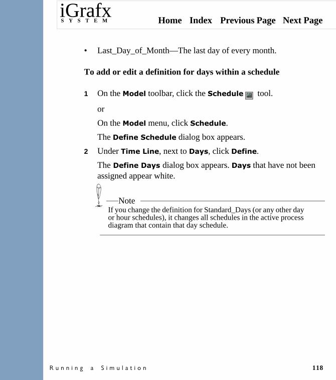
Home Index Previous Page Next PageiGrafxS Y S T E M
� � � � � � � � � � � � � � � � � � 118
• Last_Day_of_Month—The last day of every month.
To add or edit a definition for days within a schedule
1 On the ���� toolbar, click the ������ � tool.
or
On the ���� menu, click ������ �.
The ������������ � dialog box appears.
2 Under ��!��.��, next to ��$�, click �����.
The���������$��dialog box appears. ��$� that have not been assigned appear white.
NoteIf you change the definition for Standard_Days (or any other day or hour schedules), it changes all schedules in the active process diagram that contain that day schedule.

Home Index Previous Page Next PageiGrafxS Y S T E M
� � � � � � � � � � � � � � � � � � 119
Defining Hours
The following definitions are used to define the hours in resource or activity schedules:
• Standard_Hours—The time periods are 8:00 am to 12:00 pm, 12:00 pm to 1:00 pm (out of service), and 1:00 pm to 5:00 pm.
• Swing_Hours—The time periods are 4:00 pm to 8:00 pm, 8:00 pm to 9:00 pm (out of service), 9:00 pm to 12:00 am, and 12:00 am to 1:00 am.
• Night_Hours—The time periods are 12:00 am to 4:00 am, 4:00 am to 5:00 am (out of service), and 5:00 am to 9:00 am.
To add or edit a definition for hours within a schedule
1 On the ���� toolbar, click the ������ � tool.
or
On the ���� menu, click ������ �.
The ������������ � dialog box appears.
2 Under ��!��.��, next to ,����, click �����.
The ������,���� dialog box appears.
You can select an existing list to edit it, or you can click ��� to create a new list.

Home Index Previous Page Next PageiGrafxS Y S T E M
� � � � � � � � � � � � � � � � � � 120
Defining Composite Schedules
A composite schedule is a combination of existing schedules and lists of days and hours (some of which may be inactive) that creates a new schedule. You can edit an existing schedule or combine schedules to create a composite schedule.
Creating a composite schedule can save you time because it takes advantage of predefined components such as holidays. For example, a Swing_With_Holidays schedule is a composite schedule. It consists of the Swing schedule with US_Holidays schedule excluded. When a composite schedule is created, the days and hours form a mask or an overlay on the schedule, depending on whether the hours and days are active or inactive.
To define a new schedule, create a new schedule, or pick and choose among existing schedules, and then add different active or inactive hours to make a new schedule.
To create a composite schedule
1 On �������� toolbar, click the ������ � tool.
or
On the ���� menu, click ������ �.
2 In the ������������ � dialog box, under ��!��.��, click ��!������.
The +������!������������� � dialog box appears.

Home Index Previous Page Next PageiGrafxS Y S T E M
� � � � � � � � � � � � � � � � � � 121
Defining Event Schedules
An event schedule is a list of specific points in time, as compared to a regular schedule that includes time spans. You use an event schedule when you want to designate an event that happens at a specific time, for example, a batch process.
To define an event schedule
1 On the ���� toolbar, click the +"�� tool.
or
On the ���� menu, click +"��.
The ������+"�� dialog box appears. A list of existing events is displayed.
2 To see the definition for an existing event, click to select it.
The dialog box is updated to show the weekly or monthly calendar that displays the event. You can view the hours of the event by clicking a specific day in the calendar.
You can select an existing list to edit it, or click ��� to create a new event.

Home Index Previous Page Next PageiGrafxS Y S T E M
� � � � � � � � � � � � � � � � � � 122
Defining Hours for Events
You can set the following parameters to define event hours:
• Morning. 8:00 am.• Afternoon. 1:00 pm.• End_of_Day. 5:00 pm.
Defining Schedules for Events
You can set the following parameters to define event schedules:
• Every_Morning—An event happens every morning. • Every_Afternoon—An event happens every afternoon. • Every_End_of_Day—An event happens every End_of_Day. • Weekly—An event happens Monday morning of every week. • First_of_Month—An event happens on the first morning of every
month.• Last_of_Month—An event happens on the last morning of every
month.
Defining Days for Events
Event days are defined the same as days.

Home Index Previous Page Next PageiGrafxS Y S T E M
� � � � � � � � � � � � � � � � � � 123
Opening Multiple Scenarios
You can create multiple scenarios to compare models. A model consists of one or more process diagrams, reports, and scenario data. If you find that you make many changes to the scenario data between simulations, you can use multiple scenarios to save time. You can create two or more versions of the scenario data to compare the results of such things as changing the number of transactions generated or the value of an attribute.
The run setup, generators, resources, schedules, initializations, function definitions, and monitoring information apply only to a single scenario. You must supply this information for each scenario (or use the defaults). Process diagrams form the base for all of the scenarios. The only differences are the scenario data; for example, the function definitions or the generators.
To open a new scenario
1 On the �� � menu, click ��!�����.
2 In the ��!����� dialog box, click &� , and then click �������.
3 To close the ��!����� dialog box, click � ���.

Home Index Previous Page Next PageiGrafxS Y S T E M
� � � � � � � � � � � � � � � � � � 124
To copy scenario data
When you open a new scenario, it contains the system defaults. If you have set up a scenario and want to use it as the basis for a new scenario, you can use the ���$ and ����� buttons.
1 On the �� � menu, click ��!�����.
2 In the ��!����� dialog box, select the name of the scenario that you want to copy.
3 Click ���$.
To paste scenario data
After you copy a scenario to the clipboard, you can paste it to create a new scenario.
1 In the �������� dialog box, click �����.
This pastes a copy of the scenario information on the clipboard to create a new scenario. The new scenario is the last number in the sequence (for example, Scenario4 if there were previously three scenarios).
The ����� button appears only if a scenario has been copied to the clipboard. You can also copy and paste scenarios between files.
2 Double-click the new scenario name.
This opens the copied scenario.

Home Index Previous Page Next PageiGrafxS Y S T E M
� � � � � � � � � � � � � � � � � � 125
To delete or rename a scenario
1 On the �� � menu, click ��!�����.
2 Select the scenario that you want to delete or rename.
To delete, click �� ���. To rename, click ���!�. The name can contain as many as 64 alphanumeric characters, including underscore and space characters.
Using the Scenario Window
The scenario window lists all of the scenario data that you can set with the tools using the ���� menu or the ���� toolbar (Run Setup, Generators, Resources, and so forth).
Use the scenario window to set global aspects of simulation. The scenario window is in outline form. Click the � �� icon to expand or the ���� icon to collapse a topic. After you expand a topic, you can double-click any item to display the dialog box to change its value. After you set global data, on the ���� menu, point to ��, and then click ����� to begin the simulation.
Home Index Previous Page Next PageiGrafxS Y S T E M
� � � � � � � � � � � � � � � � � � 126
To open the scenario window or view a scenario
1 On the ���� toolbar, click the �������� tool.
or
On the �� � menu, click ��!�����.
The ��!����� dialog box appears with a list of available scenario names.
2 Double-click the name of the scenario you want to open, typically �������2.
or
Select the name and click (�� .
The Scenario window opens. You can click the outline buttons to expand and contract them. Some categories are unavailable because their members are not used in any activities.
NoteAfter you have a window open, use the Windows menu to view it.
You can delete unused data whenever it is no longer needed. For example, if you created a function that is no longer used, its definition is kept in the scenario window for later use but it is dimmed. You can delete it by selecting the definition and pressing �� ���.
Home Index Previous Page Next PageiGrafxS Y S T E M
� � � � � � � � � � � � � � � � � � 127
To copy and paste scenario data
To copy scenario data, for example, a generator definition or schedule, into another process diagram, follow these steps.
1 In the ������� window, click to expand the topic so that you can view the data that you want to copy.
2 Click to select the data.
3 On the +��� menu, click ���$.
4 Open the ������� window in another process diagram.
5 Click to expand this topic to view the data that matches what you have copied to the clipboard.
6 On the +��� menu, click �����.
About the Generator Timeline
The timeline is a visual method for checking the simulation time. It appears after you have defined a custom starting or ending time. The top half of the timeline shows units of simulated time. A red line marks the actual length of the simulation as set in the control data. The bottom half of the timeline indicates how long the generator is going to issue transactions.
For information on setting a resource’s overtime rate and maximum amount.

Home Index Previous Page Next PageiGrafxS Y S T E M
� � � � � � � � � � � � � � � � � � 128
Arranging Windows
After you open any of the iGrafx Process 2000 windows, you can use the Window menu to arrange the windows on the screen or to view them one at a time. The %��� menu contains standard Windows items.
If you close a process, scenario, or report window, you can open it by clicking ��!����� on the �� � menu, selecting a process, scenario, or report, and then clicking (�� .
For information on setting a resource’s overtime rate and maximum amount.

Home Index Previous Page Next PageiGrafxS Y S T E M
� � � � � � � � � � � � � � 129
Using Trace Mode
Using Trace Mode with Process Diagrams
Trace mode graphically traces a simulation (the flow of transactions through a process diagram). The shapes for each activity change color as transactions move through them. Trace mode lets you troubleshoot a model by simply watching the transactions in the trace window – you can see how the model is working and identify problem areas.
Trace Mode Features
The trace mode allows you to do the following:
• Visually track how a process diagram is transacted• Use colors to display the state of an activity• Set pause points that let you run the simulation to a pause point
and then you can examine the status of individual settings• View or set the value of transaction and global attributes during
the simulation• Quickly identify problem areas in a process diagram• Track transaction paths• Quick what-if analysis by modifying attributes• Trace a simulation in normal (graphical) view• Trace a simulation in tabular view

Home Index Previous Page Next PageiGrafxS Y S T E M
� � � � � � � � � � � � � � 130
Entering and Exiting Trace Mode
Enter and exit trace mode by selecting a process diagram, and then selecting the ����� command. Access the ����� command by doing the following:
On the ���� menu, point to ��, and then click �����.
or
On the ���� menu, click the ����� tool.
TipAll diagrams in the file enter or exit trace mode when you click the trace tool.
Using the Trace Toolbar
The following tools are located on the ����� toolbar and are used to control the trace of a simulation:
Tool Command Description
Start Starts the simulation.
Step Steps through the simulation.
Pause Pauses the simulation.

Home Index Previous Page Next PageiGrafxS Y S T E M
� � � � � � � � � � � � � � 131
To enable trace mode
1 On the %��� menu, select a process diagram.
or
On the ��� menu, click ���, and select a process diagram.
2 On the ���� menu, point to ��, and click �����.
or
On the ���� toolbar, click the ����� tool.
TipIf you have a process diagram in trace mode, you must exit trace mode before you can place another process diagram in trace mode.
Resume Resumes the simulation.
Go to Pause Runs the simulation until you encounter a pause point. Click Go to Pause again to resume the simulation.
Stop Stops the simulation.
Speed Slider
Increases or decreases the simulation speed.

Home Index Previous Page Next PageiGrafxS Y S T E M
� � � � � � � � � � � � � � 132
The active window goes into trace mode.
TipUse the trace mode with a process diagram in normal or tabular view.
To display the trace toolbar
1 From the (�� menu, click ��� #���.
2 In the ��� #��� dialog box, select the ������box.
To set the viewing percentage
1 Use the (�� list box on the ������� toolbar.
or
From the (�� menu, click 7��!.
2 In the 7��! dialog box, set the viewing percentage.
NoteIf you select All and change the size of the process window while in trace mode, the program recalculates the percentage and continues to display the entire process diagram.
3 To use the entire window, click the ��*�!�1� icon.

Home Index Previous Page Next PageiGrafxS Y S T E M
� � � � � � � � � � � � � � 133
To start and stop the simulation while in trace mode
To start the simulation, click the ����� tool on the ���� toolbar.
TipTo keep the report window from displaying on top of the process diagram after the simulation has completed, click Minimize on the report window, and convert it into an icon.
To stop the simulation, click the ���� �tool.
To pause and resume a simulation while in trace mode
1 On the ���� toolbar, click the ����� �tool.
The simulation pauses.
2 On the ���� toolbar, click the �����0����!� �tool.
The simulation resumes.
To increase or decrease the simulation speed while in trace mode
To increase or decrease the simulation speed, move the slider.

Home Index Previous Page Next PageiGrafxS Y S T E M
� � � � � � � � � � � � � � 134
To run a simulation until a pause point is encountered while in trace mode
1 Select the shape containing the activity you would like to pause.
2 On the ����� menu, click �������������� to insert a condition that causes the simulation to pause.
3 To start or resume the simulation and watch the shapes change colors, click the �����0����!� tool.
or
To start or resume the simulation until the next pause is encountered, click the ����������� tool.
The simulation resumes at maximum speed. The shapes will not change color until the simulation pauses.
To exit trace mode
On the ���� toolbar, click the ����� tool.
Setting Trace Colors
Trace colors are used to display the status of an activity during the simulation of a process diagram that is in trace mode. Select the ������
�� ��� command on the ����� menu to modify the trace colors.

Home Index Previous Page Next PageiGrafxS Y S T E M
� � � � � � � � � � � � � � 135
To change the trace colors
1 On the ����� menu, click ����� �� ���.
2 On the ����� �� ��� dialog box, use the scrolling lists to choose the new colors.
3 Click ��.
NoteYou can use the trace window to view more than one process.
Using the Trace Numbers
During the simulation of a process diagram that is in trace mode, inside each shape trace numbers may appear. The trace numbers provide detailed information about the transaction status. The transaction status is indicated by the color of the shape during the trace. When more than one transactions accumulate for processing at any activity, the trace numbers display the total number of transactions at the activity and the number of transactions that are in the shown state. Only one trace color appears in an activity at any one moment.
For example, at the following activity, fifteen total transactions have accumulated, and five are being worked. The trace numbers 5/15 appear inside the shape.

Home Index Previous Page Next PageiGrafxS Y S T E M
� � � � � � � � � � � � � � 136
TipYou can also check the state of the other transactions.
Using the Transactions Window
When you enable trace mode, the Transactions window appears. During a simulation, use this window to:
• View transaction status and data while the simulation runs.• View transaction attributes values.• Modify transaction attributes values to validate the data in your
process diagram.
Reviewing and Modifying Transaction Attribute Data
The left side of the window sequentially numbers and displays the data for the transactions as they flow through the process diagram. Each transaction is on separate row. The column headings for the window include the names of the transaction attributes assigned to the transaction. To modify a transaction attribute, double-click on the cell you want to modify.

Home Index Previous Page Next PageiGrafxS Y S T E M
� � � � � � � � � � � � � � 137
TipTo display the transaction attributes column headings in the Transactions window, click the right mouse button in the window, and click Attributes on the shortcut menu.
Reviewing and Editing Resource Data
The right side of the transaction window displays resource information for each transaction. Modify these settings by double-clicking on the value that you want to modify.
To open and close the Transactions window
1 On the ���� toolbar, click the ����� tool.
2 On the (�� menu, click ����������.
To review or modify transaction attributes in the Transactions window
1 On the ���� toolbar, click the ����� tool.
2 On the (�� menu, click ����������.
The Transactions window appears.
3 Right-mouse click the Transactions window, and click �����#���� on the shortcut menu.
Home Index Previous Page Next PageiGrafxS Y S T E M
� � � � � � � � � � � � � � 138
The column headings for the attribute values appear in the Transactions window.
4 Click the ����� tool to start the simulation.
Transactions, their attributes, and resource data appears in the ���������� window.
5 Click the ����� �tool.
6 To modify the transaction attribute associated with a transaction, double-click the value in the appropriate column in the Transactions window.
NoteChanging the duration transaction attribute does not affect the current activity.
7 Click the ���� �tool to end the simulation.
or
Click the ����!�0����� tool to restart the simulation, and
repeat steps 4 – 6.

Home Index Previous Page Next PageiGrafxS Y S T E M
� � � � � � � � � � � � � � 139
Using the Global Attributes Window
While in trace mode, you can display this window by clicking �����#���� on the (�� menu. During a simulation, use this window to:
• View global transaction attribute data while the simulation runs.• Modify global transaction attributes values to validate the data in
your process diagram.
To open and close the Attributes window
1 On the ���� toolbar, click the ����� tool.
2 On the (�� menu, click �����#����.
To review or modify global attribute values during a simulation
1 On the ���� toolbar, click the ����� tool.
2 On the (�� menu, click �����#����.
The Attributes windows appears.
3 Click the ����� �tool to start the simulation.
The global attributes (scenario, process, and department attributes) settings appear in the Attributes window during this simulation.
4 Click the ����� �tool.

Home Index Previous Page Next PageiGrafxS Y S T E M
� � � � � � � � � � � � � � 140
5 To modify the global attribute associated with a transaction, double-click the value in the appropriate column in the Attributes window.
6 Click the ���� tool to end the simulation.
or
Click the ����!�0����� tool to restart the simulation, and
repeat steps 4 – 6.
7 To remove the attribute window, click �����#���� on the (�� menu.
Using Pause Points and the Pause Points Window
A pause point is a breaking position that you can place in a trace simulation. When you run a trace, transactions stop at any pause points. You can use this break to examine attributes or values associated with the transaction.
To insert a pause point
1 In the trace window, highlight the activity for the pause point.
2 On the ����� menu, click ��������������.
The �������������� dialog box appears.
To always pause the simulation when a transaction reaches this point, click � �$�.

Home Index Previous Page Next PageiGrafxS Y S T E M
� � � � � � � � � � � � � � 141
To conditionally pause the simulation based on an expression evaluating to true, click +*������������.
The expression builder appears. Insert an expression. For example, in the following expression, the trace pauses if an attribute named ������$�� is set to %��������.
To pause the simulation after a specified count of transactions reaches this point, click ����������.
A scrolling counter appears. Enter a count. When the number of transactions through the activity equals the count, the next transaction pauses.
3 Click ��.
To use pause points to start and stop a simulation
1 Click the ����������� tool to go to a pause point.
This runs the simulation at its fastest speed (not changing the colors) until it reaches the pause point. This is a useful time-saver when the point that you wish to analyze occurs well into the simulation.
2 Click the ����!�0����� tool to continue past a pause point.
OrderType = WestCoast

Home Index Previous Page Next PageiGrafxS Y S T E M
� � � � � � � � � � � � � � 142
To edit a pause point
1 On the (�� menu, click �����������.
2 In the ����������� window, double-click a pause point to edit it using the �������������� dialog box.
3 To activate a pause point, select the check box in the ����"� column.
To activate or deactivate a pause point
1 On the (�� menu, click ����� �����.
2 In the ����� ����� window, select the box in the Active column to activate or clear the box to deactivate.
To delete pause points
1 On the (�� menu, click������ �����.
2 In the ����� ����� window, click to select the pause point definition.
3 On the ����� menu, click �� ��� ����� ����.
or
On the ����� menu, click �� ��� � ������������.
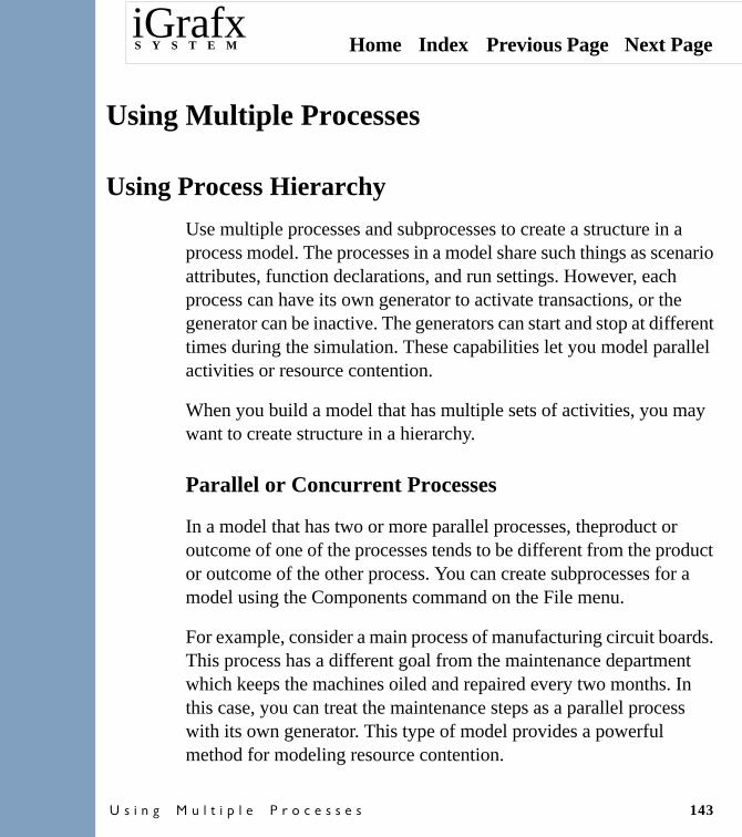
Home Index Previous Page Next PageiGrafxS Y S T E M
� � � � � � � � � � � � � � � � � � � � � � 143
Using Multiple Processes
Using Process Hierarchy
Use multiple processes and subprocesses to create a structure in a process model. The processes in a model share such things as scenario attributes, function declarations, and run settings. However, each process can have its own generator to activate transactions, or the generator can be inactive. The generators can start and stop at different times during the simulation. These capabilities let you model parallel activities or resource contention.
When you build a model that has multiple sets of activities, you may want to create structure in a hierarchy.
Parallel or Concurrent Processes
In a model that has two or more parallel processes, theproduct or outcome of one of the processes tends to be different from the product or outcome of the other process. You can create subprocesses for a model using the Components command on the File menu.
For example, consider a main process of manufacturing circuit boards. This process has a different goal from the maintenance department which keeps the machines oiled and repaired every two months. In this case, you can treat the maintenance steps as a parallel process with its own generator. This type of model provides a powerful method for modeling resource contention.

Home Index Previous Page Next PageiGrafxS Y S T E M
� � � � � � � � � � � � � � � � � � � � � � 144
Subprocesses
Subprocesses are often created for organizational reasons. For example, if you have different audiences for segments of the process diagram, you can define the highest-level activities in the main process diagram and define subordinate activities as subprocesses, as shown in the following illustration.
Working with Processes
Every file containing a process diagram contains at least one process. If you are working with multiple processes, you create the processes within the same file for use as either concurrent processes or subprocesses.
To create a new process
1 On the �� � menu, select ��!�����.
The ��!����� dialog box appears.
TipClick the / button to expand an item.
2 Select how to view the components.
� ��!�����. All of the processes in the file are listed in alphabetical order.

Home Index Previous Page Next PageiGrafxS Y S T E M
� � � � � � � � � � � � � � � � � � � � � � 145
���-��! ,�������$. The relationships between the processes are shown.
���-��!�4��$���������������!���. This is a list of all departments in the file. You can expand a department to view the processes in which each department is used.
3 To create a new process, click &� , and select �������.
To create a new process based on a template, click &� , and select &� ����!���!� ���. In the &� ���!��������!���!� ��� dialog box, select a template and a component.
To rename a process, select a process from the list, click ���!�, and change its name. For example, you can rename �������2 to Engineering.
To copy a process, select a process from the list, and then click ���$. Click ����� to copy the contents of the clipboard into a new process.
To view hierarchy in a process diagram
1 On the �� � menu, click ��!�����.
2 In the ��!����� dialog box, select the ���-��! ,�������$ option to view the relationships between different processes.
The process hierarchy appears in the dialog box.
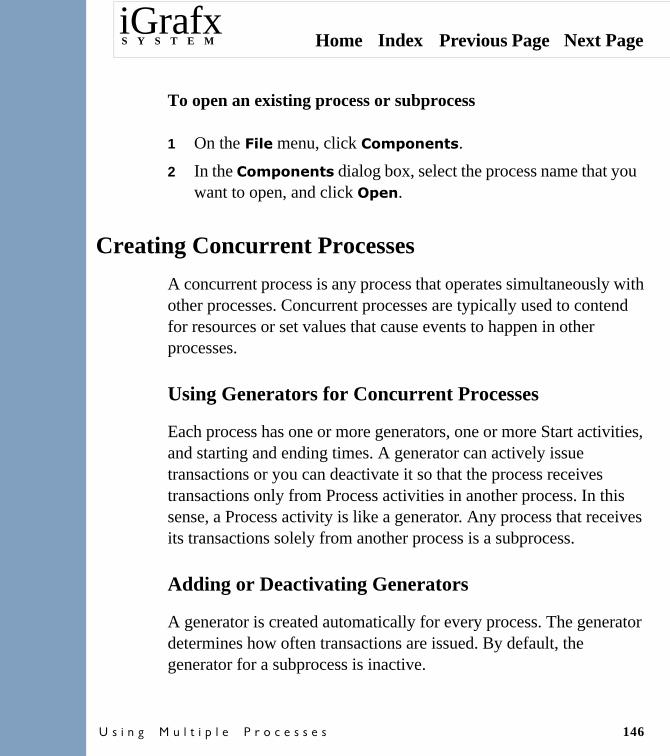
Home Index Previous Page Next PageiGrafxS Y S T E M
� � � � � � � � � � � � � � � � � � � � � � 146
To open an existing process or subprocess
1 On the��� � menu, click ��!�����.
2 In the ��!����� dialog box, select the process name that you want to open, and click ���.
Creating Concurrent Processes
A concurrent process is any process that operates simultaneously with other processes. Concurrent processes are typically used to contend for resources or set values that cause events to happen in other processes.
Using Generators for Concurrent Processes
Each process has one or more generators, one or more Start activities, and starting and ending times. A generator can actively issue transactions or you can deactivate it so that the process receives transactions only from Process activities in another process. In this sense, a Process activity is like a generator. Any process that receives its transactions solely from another process is a subprocess.
Adding or Deactivating Generators
A generator is created automatically for every process. The generator determines how often transactions are issued. By default, the generator for a subprocess is inactive.

Home Index Previous Page Next PageiGrafxS Y S T E M
� � � � � � � � � � � � � � � � � � � � � � 147
To add or deactivate a generator
On the ���� menu, click ���������.
The��������������� dialog box appears.
NoteEach generator introduces transactions into the process according to the instructions in its generator definition. For example, one generator can issue transactions every two and four days, and in the same process, another generator can issue transactions every day.
If you want a process to receive transactions only from a Process activity, you can deactivate or delete the generator.
If the subprocess also operates as an independent process, you can leave the generator active.
Using Subprocesses
To create hierarchy in a process diagram, you can use subprocesses. The top-level process typically contains high-level activities, with other subprocesses containing the subordinate activities.
In a hierarchical process diagram, the generator for a subprocess is typically inactive. Transactions are issued instead by higher-level Process activities in another process.

Home Index Previous Page Next PageiGrafxS Y S T E M
� � � � � � � � � � � � � � � � � � � � � � 148
Some overhead is associated with multiple processes, mostly in the time it takes for you to create the diagrams, but also in maintenance and simulation time. This is a trade-off to be considered if you are creating a large number of hierarchical layers (10 or more).
To view a subprocess
Select the activity that contains the subprocess, press the ����� key, and double-click the mouse.
or
On the��� � menu, click ��!�����, and select a subprocess from the list of Processes in the ��!����� dialog box.
The subprocess appears in a window.
TipTo quickly find all the Process activities, on the Edit menu, click Select. Use the Select dialog box to select all Process activities.
Private and Non-Private Subprocesses
The transactions in a non-private subprocess interact with other transactions while those in a private subprocess do not. Private subprocesses ensure that transactions are kept separate for purposes of splitting and joining.

Home Index Previous Page Next PageiGrafxS Y S T E M
� � � � � � � � � � � � � � � � � � � � � � 149
Assume you have two processes that use the same subprocess for creating a technical document. The Process activity Create document is the same for both processes.
Although the subprocess is the same, the transactions are kept apart. By using a private subprocess, you ensure that a joining activity collects the correct document chapters for the parent process.
Tips for Working with Multiple Processes
Before you create a new process, assign unique names to any departments that will not be shared. Otherwise, all departments with the same name are considered to be the same department across the processes. For example, a newly-created process had a department name Dept. 1 that is a shared department with Dept. 1in all other processes. A shared department uses the same resources and attributes for simulation purposes.
After a department is shared, any change to the name affects all the shared department names in all processes.
Linking and Unlinking Department Names
When two or more departments have the same name, the departments are linked (when you edit one name, it changes all other departments with the same name). After department names are linked, you can unlink them.

Home Index Previous Page Next PageiGrafxS Y S T E M
� � � � � � � � � � � � � � � � � � � � � � 150
To unlink departments
1 Select the department.
2 Use the backspace key to delete all the characters in the department name.
NoteBe sure to delete all spaces.
3 Deselect the department.
Now you can make changes to the department name without affecting the other departments.
Windowing Techniques
The Window menu items are useful for viewing windows containing different processes. For example, you can have windows open for two processes and then select Tile Horizontal from the Window menu. This creates a horizontal configuration that enables you to view both processes. If you have other windows open, you can turn them into icons so that they do not block other windows.

Home Index Previous Page Next PageiGrafxS Y S T E M
� � � � � � � � � � � � � � � � � � � � � � 151
To use trace mode to view multiple processes
1 On the ���� menu, point to ��, and then click ����� to place �������2 in trace mode.
2 On the %��� menu, click %��� to create a copy of the active window.
3 On the �� � menu, click ��!�����.
4 In the ��!����� dialog box, select a process under the ���-��!� category, and click (�� .
The process appears in a window.
5 Select another process to view, or click � ���.
To build a process hierarchy
You can copy existing process diagrams into a single process diagram to build a hierarchical process diagram (a process that contains subprocesses).
1 On the �� � menu, click &� , and point to ������� to create a new, untitled process diagram that will represent the highest-level for activities in your process.
2 On the �� � menu, click ��!�����.
3 In the ��!����� dialog box, click &� , and select �������.
A new process diagram is created and appears in a window.
4 On the �� � menu, click ��"�.

Home Index Previous Page Next PageiGrafxS Y S T E M
� � � � � � � � � � � � � � � � � � � � � � 152
For example, save the process diagram using the name ���.
5 (Optional) Draw symbols to represent the highest-level activities.
Later, after the subprocesses have been created, you can specify which symbol references a subprocess using the ���������� command (�������������� �-�#�*�)��������#).
6 On the �� � menu, click &� to create a second process diagram.
For example, open a file that you have already created for the �� �� department.
7 On the %��� menu, select �� ��,���1��� $ (or �������) to view both process diagrams.
8 Activate the window containing the second process diagram (�� ��.)
9 On the �� � menu, click ��!�����.
10 In the Components dialog box, select the process �� ��, and click ���$.
This copies the contents of the �� �� process diagram to the clipboard.
11 Click to select the process for ���. (Process1).
12 Click �����.
This copies the clipboard (the Sales process diagram) into �������3 in the original file contains Top. You can repeat the steps to copy other existing files into new processes.
13 Activate the first window and create process activities for the other processes.

Home Index Previous Page Next PageiGrafxS Y S T E M
� � � � � � � � � � � � � � � � � � � � � � 153
You do this by double-clicking on an activity and specifying process information on the ���� tab.
14 One at a time, activate each of the subprocesses, and on the ���� menu, select ���������.
15 In the ��������� dialog box, specify that the generator for each subprocess in not ����"�.

Home Index Previous Page Next PageiGrafxS Y S T E M
� � � � � � � � � � � � � 154
Using Monitors
Using Monitors to Collect Data
A monitor is a data filter that you can place on any activity in the process diagram to collect data. The types of data include basic transaction statistics such as busy and waiting time, number of transactions, or the value of attributes at certain points.
Monitors provide a method of validating a model by checking intermediate statistics. For example, you can place a monitor to tabulate the number of transactions that reach an activity. You can also use starting and ending monitors to gather data about a specific segment of the process flow.
A monitor collects statistics about transactions and attribute data. The statistics are gathered at the activities that you specify in the process diagram. Monitors can collect the following data.

Home Index Previous Page Next PageiGrafxS Y S T E M
� � � � � � � � � � � � � 155
Evaluating Monitors
Monitors are evaluated during simulation at the start of an activity. This affects monitor statistics because the activity containing the monitor is not included in the statistics. For example, if a monitor keeps track of basic statistics such as service time and busy time, it does not include time statistics for the activity on which the monitor is placed.
Data Type Description
Count Counts the transactions at a specific point to track how many times a transaction reached an activity. This can represent scrapped units or canceled orders.
Basic transaction statistics
Collects basic statistics either between two points or from the start point to the current monitor. You can use this to collect statistics such as service time or waiting time between two points. For information on these statistics.
Filtered data Further filters the data, for example, how many transactions matched a specific attribute value.
Accumulated values
A value that cumulatively increases every time a transaction passes through the activity.

Home Index Previous Page Next PageiGrafxS Y S T E M
� � � � � � � � � � � � � 156
Viewing Monitor Statistics
After you run a simulation, you can view monitor results in the Report window by adding a report element. You can add the element to any of the tabs, for example, the Custom tab. In the report element, you specify statistics specifically gathered by monitors.
Identifying Monitors in the Tabular View
Activities with monitors placed on them have a monitor indicator displayed to the left of the activity.
To define a monitor
1 Select the activity at which to place a monitor.
2 On the ���� toolbar, click the ������ tool.
or
On the ���� menu, click �������.
The ������������� dialog box appears. This dialog box contains a list of monitors that exist in the model.
The number after a monitor name indicates the number of placements of the monitor. For example, ���� (1) indicates that the Test monitor has been placed on one activity.
3 To add a new monitor, click ���.

Home Index Previous Page Next PageiGrafxS Y S T E M
� � � � � � � � � � � � � 157
The ����&� ������� dialog box appears. Use this dialog box to specify the monitor name and type.
or
To modify a monitor, select it and click �����$.
The �����$���������$�� dialog box appears. Use this dialog box to modify the monitor type.
To place a monitor
1 Select the shape that contains the activity at which you want to place the monitor.
2 On the ���� menu, click ������, or click the ������ tool
on the ���� toolbar.
3 In the ������������� dialog box, define a monitor or select an existing monitor from the list.
4 Click � ���.
A number appears after the monitor name, indicating the number of times the monitor has been placed.

Home Index Previous Page Next PageiGrafxS Y S T E M
� � � � � � � � � � � � � 158
To find a monitor
1 On the ���� menu, click ������.
or
On the ���� toolbar, click the ������ tool.
2 In the ������������� dialog box, click the monitor name you want to find.
3 Click ���.
The ������� dialog box closes, and the activity containing the monitor is selected.
4 Use the ������ tool on the ���� �- toolbar to modify, delete, remove, or place the monitor on a different activity.
To find multiple occurrences of a monitor
1 On the ���� menu, click ������.
or
On the ���� toolbar, click the ������ tool.
2 In the ������������� dialog box, click the monitor name that you want to find.
A number appears after the monitor name, indicating the number of times the monitor has been placed.
3 Click ���.
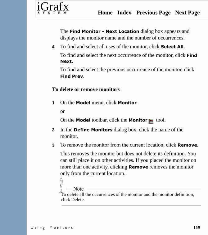
Home Index Previous Page Next PageiGrafxS Y S T E M
� � � � � � � � � � � � � 159
The �����������)�&�*��.������ dialog box appears and displays the monitor name and the number of occurrences.
4 To find and select all uses of the monitor, click �� ����� .
To find and select the next occurrence of the monitor, click ����
&�*�'
To find and select the previous occurrence of the monitor, click ��� ���".
To delete or remove monitors
1 On the ���� menu, click ������.
or
On the ���� toolbar, click the ������ tool.
2 In the ������������� dialog box, click the name of the monitor.
3 To remove the monitor from the current location, click ��!�"�.
This removes the monitor but does not delete its definition. You can still place it on other activities. If you placed the monitor on more than one activity, clicking ��!�"� removes the monitor only from the current location.
NoteTo delete all the occurrences of the monitor and the monitor definition, click Delete.

Home Index Previous Page Next PageiGrafxS Y S T E M
� � � � � � � � � � � � � � � � 160
Reporting Results
Reviewing Simulation Report Results
When you run a simulation, statistics are gathered about process times, costs, resource utilization, and queues. These statistics are categorized by transaction, activity, resource, or monitor.
You can use custom statistics to create unique combinations of the standard statistics (for example, setting costing information or revenue formulas). Custom statistics are updated and calculated automatically with each simulation.
You can maintain several sets of named simulation data to compare results across simulation runs and scenarios.
After a simulation runs, use the Run command or the Trace command on the Model menu to update the data in the report window with the results of the simulation.
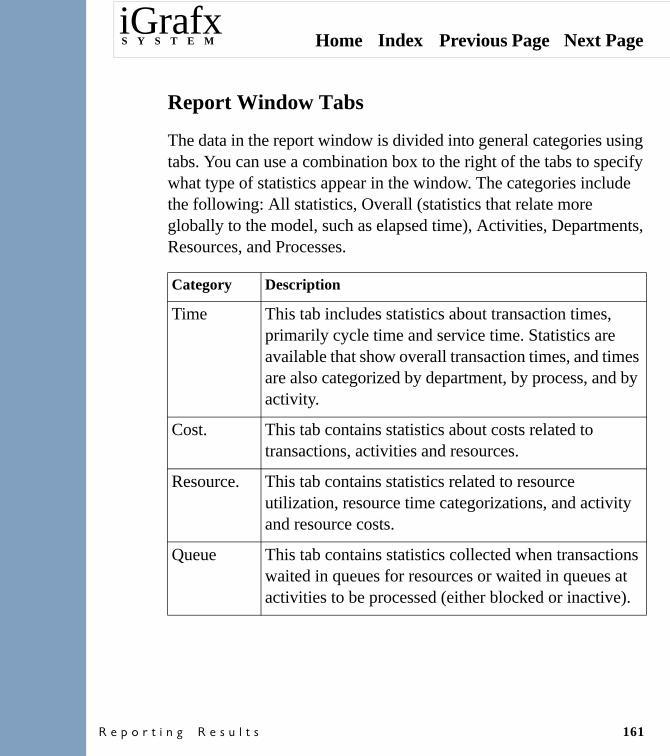
Home Index Previous Page Next PageiGrafxS Y S T E M
� � � � � � � � � � � � � � � � 161
Report Window Tabs
The data in the report window is divided into general categories using tabs. You can use a combination box to the right of the tabs to specify what type of statistics appear in the window. The categories include the following: All statistics, Overall (statistics that relate more globally to the model, such as elapsed time), Activities, Departments, Resources, and Processes.
Category Description
Time This tab includes statistics about transaction times, primarily cycle time and service time. Statistics are available that show overall transaction times, and times are also categorized by department, by process, and by activity.
Cost. This tab contains statistics about costs related to transactions, activities and resources.
Resource. This tab contains statistics related to resource utilization, resource time categorizations, and activity and resource costs.
Queue This tab contains statistics collected when transactions waited in queues for resources or waited in queues at activities to be processed (either blocked or inactive).
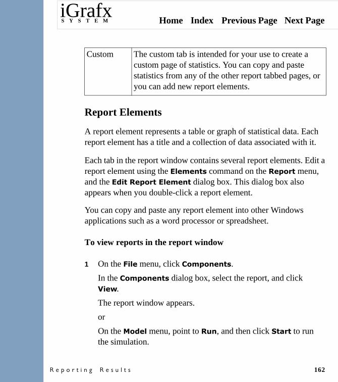
Home Index Previous Page Next PageiGrafxS Y S T E M
� � � � � � � � � � � � � � � � 162
Report Elements
A report element represents a table or graph of statistical data. Each report element has a title and a collection of data associated with it.
Each tab in the report window contains several report elements. Edit a report element using the + �!��� command on the ������ menu, and the +�����������+ �!�� dialog box. This dialog box also appears when you double-click a report element.
You can copy and paste any report element into other Windows applications such as a word processor or spreadsheet.
To view reports in the report window
1 On the �� � menu, click ��!�����.
In the ��!����� dialog box, select the report, and click (�� .
The report window appears.
or
On the ���� menu, point to ��, and then click ����� to run the simulation.
Custom The custom tab is intended for your use to create a custom page of statistics. You can copy and paste statistics from any of the other report tabbed pages, or you can add new report elements.

Home Index Previous Page Next PageiGrafxS Y S T E M
� � � � � � � � � � � � � � � � 163
When the simulation is complete, the report window appears.
TipIf the report window is obscured or not displayed, on the Window menu, click the Report window.
2 Select a report tab in the report window.
The ����� � button appears on the tabbed report window when you modify any of the settings for the default report elements. Click ����� � to return the element settings to their default values. You can change, delete, or add elements to a report, or open other reports. If you add report elements after you run a simulation, you can view the new statistics without re-simulating. However, if you change the process diagram or scenario information, you must simulate again to view new results.
TipTo see report results for new attributes, monitors, or other changes that you made to the process diagram or scenario information, you must run the simulation again.

Home Index Previous Page Next PageiGrafxS Y S T E M
� � � � � � � � � � � � � � � � 164
To edit a report element
You can change the contents or structure of a report element in any of the tabbed pages of the Report window.
1 Double-click the report element.
or
Right-mouse click the report element, and click +��� ������.
The�+�����������+ �!�� dialog box appears.
2 Use the dialog box to modify the report element.
To add a new report element
1 Select the report element, and click ����+ �!�� on the ������� menu.
or
Right-mouse click the report element, and click ����+ �!��.
The ��������� dialog box appears.
2 Use this dialog box to define the statistics in the report element.
3 Click &�*�.
The ��������� dialog box appears.
4 Use this dialog box to define column labels and row legends for the statistic.
This dialog box contains the same information as the ��������� tab on the�+�����������+ �!���dialog box.
Home Index Previous Page Next PageiGrafxS Y S T E M
� � � � � � � � � � � � � � � � 165
5 Click &�*�.
The �� ���� dialog box appears.
6 Use this dialog box to define how to filter the statistic.
This dialog box contains the same information as the �� ���� tab on the +�����������+ �!�� dialog box.
7 Click &�*�.
The ���!��� dialog box appears.
8 Use this dialog box to define how to format and sort the statistic.
This dialog box contains the same information as the ���!��� tab on the�+�����������+ �!�� dialog box.
9 Click �����.
Using the Report Window to Review Transaction Statistics
You can use transaction statistics to analyze the time and cost of transactions in the model. Transaction statistics are calculated only for transactions that finish processing, either by completing the flow through the process diagram or by reaching an activity that has no further connections.

Home Index Previous Page Next PageiGrafxS Y S T E M
� � � � � � � � � � � � � � � � 166
In the default Report window, both the ��!� and ���� tabs have report elements containing transaction statistics. (You can also add your own report elements to any tab or create additional reports.)
NoteOnly completed transactions are included in transaction statistics.
If a model uses multiple processes to create hierarchy, the transaction statistics, by default, combine the results of all processes. For example, the transaction count is equal to the total number of transactions in all processes. You can change the row legends of the report element to view the results of a specific process.

Home Index Previous Page Next PageiGrafxS Y S T E M
� � � � � � � � � � � � � � � � 167
Transaction Formulas
You can use the following calculations to process transaction statistics:
Calculation Description
Total (Tot) The combination of all of the completed transaction statistics. If you apply a filter to the statistic, then only specific, completed transactions are counted.
Average (Avg)
The total divided by the count of completed transactions. If you apply a filter, then only specific, completed transactions are counted (same as totals).
Total # Transactions (#Trans)
The number of transactions that have completed the process. This does not include the transactions that are still in the process when the simulation ends. When a transaction leaves and reenters a department, it is counted only once in the department’s total. For information about viewing statistics by department,.

Home Index Previous Page Next PageiGrafxS Y S T E M
� � � � � � � � � � � � � � � � 168
Using the Report Window to Review Activity Statistics
Activity statistics are used to analyze the behavior of transactions being processed as activities.
In the Report window, the ��!�, ����, ��������, and 8���� tabs have report elements containing activity statistics. Each row of the report element is identified by the text label of the activity, with or without a department name. For example, an activity labeled Prepare report can appear in the report element as Prepare report or Dept.1- Prepare report. You can also add the process name if there is more than one process.
The order of the activities in a report element is affected by whether the report element is sorted and whether the element is hierarchical. If it is sorted, you can select the sorting format. If the element is hierarchical, the activities in each process are sorted separately. Otherwise, the regular sorting format is used.

Home Index Previous Page Next PageiGrafxS Y S T E M
� � � � � � � � � � � � � � � � 169
Formulas for Activity Statistics
The following calculations are available in many of the activity time and queue statistics.
Activity Time Statistics: Report Window - Time tab
The ��!� tab in the Report window displays activity times. Activity times are similar to transaction times, except the times are calculated for each activity as transactions are processed. The time statistics are working time, waiting for resource time, blocked time, inactive time, cycle time, service time, waiting time, and service waiting time.
Calculations Description
Total (Tot) For time statistics, the total time is calculated for each activity. If you apply a filter to the statistic, then only specific, completed transactions are counted.
Average (Avg)
For time statistics, the average is the total time for the activity divided by the count of completed transactions. For queue statistics, the denominator depends on the statistic.
Maximum (Max)
The highest number accumulated for the statistic at any one point in time (for example, the high-water mark).
Minimum (Min)
The lowest number accumulated for the statistic at any one point in time.
Home Index Previous Page Next PageiGrafxS Y S T E M
� � � � � � � � � � � � � � � � 170
Activity Cost Statistics: Report Window - Cost tab
The ���� tab in the Report window displays activity costs. Activity costs are similar to transaction costs, except the costs are calculated for each individual activity as transactions are processed. An activity can accumulate costs categorized by value type, by resource type, and by standard or overtime.
Using the Report Window to Review Resource Statistics
Resource statistics are used to analyze data that has been collected about resources, including workers and other resources that you have defined.
In the Report window, the ����, ��������, and 8���� tabs have report elements containing resource statistics.

Home Index Previous Page Next PageiGrafxS Y S T E M
� � � � � � � � � � � � � � � � 171
Resource Statistics Formulas
The following calculations are available in many of the resource statistics.
Using the Report Window to Review Resource Time Statistics - Resource tab
The ��!� tab in the Report window displays resource time statistics. During simulation, a resource can always be classified as busy, out of service, idle, or inactive. You set how a resource spends its time when you specify how activities acquire and use it, for how long, and by its schedule.
The sum of a resource’s time equals the total elapsed time of the simulation.
Calculations Description
Total (Tot) The total is the sum of time or costs accrued by the resource. If you apply a filter to the statistic, then only specific things such as departments, resources, or pools are counted. For example, totals that are filtered by department only include processing time that occurred in the department.
Average (Avg)
The total divided by the count of resources. If you apply a filter, then only specific departments, resources, or pools are counted.

Home Index Previous Page Next PageiGrafxS Y S T E M
� � � � � � � � � � � � � � � � 172
Subsets of Resource Busy Time
Resource/Time Description
Workers (Count)
The total number of workers for one or all departments.
Total Elapsed Time (Time)
The amount of time that elapsed between the simulation starting and ending times.
Busy Time (Avg Busy, Tot Busy)
The time that a resource spends working, for example, processing a transaction. This time is paid.
Out of Service Time (Avg OOS, Tot OOS)
The time that a resource is active but unavailable to process transactions. A resource can also be acquired by an activity as out of service. Out of service time can be paid or unpaid, depending on how the time span is defined in the resource’s schedule.
Idle Time (Avg Idle, Tot Idle)
The time that a resource spends available for use but not currently processing a transaction. This time is paid.
Inactive Time The remaining time when a resource is out of schedule. This time is unpaid.

Home Index Previous Page Next PageiGrafxS Y S T E M
� � � � � � � � � � � � � � � � 173
Resource/Time Description
Resource Waiting Time and Non-Waiting Time (Avg Res Wait, Tot Res Wait)-
The time that a resource spends waiting. This occurs when an activity processing a transaction acquires a resource with the Wait option, and the transaction must wait for some reason (for example, waiting for another resource, or the transaction incurs blocked or inactive time). Tot Busy = Tot Res Wait + (Total resource non-waiting time)
Resource Standard Time and Resource Overtime (Avg OT, Tot OT)
The time that a resource spends in standard time or overtime. A resource is in overtime if an activity acquires a resource and requires that it finish processing the transaction even though the resource should go out of schedule (become inactive) prior to finishing. Tot Busy = (Resource standard time) + Tot OT

Home Index Previous Page Next PageiGrafxS Y S T E M
� � � � � � � � � � � � � � � � 174
Combinations of Resource Times
Resource/Time Description
Resource Utilization (Res Util%)
The percentage of scheduled active time (when a resource should be in schedule) that a resource is busy but not out of service.
The total scheduled active time is calculated by figuring the total number of hours during which the resource is scheduled to be active during the entire simulation. For example, assume a simulation runs for two calendar days using the Standard schedule. This creates 18 hours scheduled active time and two hours out of service time (lunch breaks) for a total of 16 hours. If the total busy time for a worker is eight hours, the resource utilization is 50%.
Tot Busy(Total scheduled active time) -

Home Index Previous Page Next PageiGrafxS Y S T E M
� � � � � � � � � � � � � � � � 175
NoteIt is possible to get over 100% resource utilization because overtime can cause busy time outside of the scheduled active time.
Using the Report Window to Review Resource Cost Statistics - Cost and Resource tabs
The costs associated with a resource are specified when you define a resource and at the time when an activity uses a resource.
The resource paid times are divided into the following categories (also see the previous discussion on resource standard time in Subsets of Resource Busy Time).
Non-Waiting Resource Utilization (NW Util%)
The percentage of scheduled active time (when a resource should be in schedule) that a resource is busy but not waiting or out of service.
If the worker in the previous example has accrued two hours waiting for another resource, then the non-waiting resource utilization is 37.50%.
Tot Busy - Tot Res (Total scheduled active time) -

Home Index Previous Page Next PageiGrafxS Y S T E M
� � � � � � � � � � � � � � � � 176
A resource’s cost is the combination of standard cost, overtime cost, and any per use costs.
Resource/Time Description
Resource Standard Paid Time
A resource’s normally scheduled hours. This includes busy time, out of service time (but only if it has been marked paid in the schedule) and idle time. Resource standard paid time = Tot Busy + Tot OOS (paid) + Tot Idle.
Resource Overtime (Avg OT, Tot OT)
The amount of time that a resource worked overtime.
Resource/Time Description
Standard Cost (Avg Std Cost, Tot Std Cost)
The cost of the resource working during standard hours. This is the result of multiplying the resource’s standard paid hours by the hourly rate that is specified in the resource definition. (See above for the definition of resource standard paid time.Tot Std Cost = (Resource standard paid time) * (Resource’s standard hourly rate).
Overtime Cost (Avg OT Cost, Tot OT Cost)
The cost of the resource working during overtime. This is the result of multiplying the overtime hours by the overtime hourly rate of the resource. Tot OT Cost = Tot OT * (Resource’s overtime hourly rate).

Home Index Previous Page Next PageiGrafxS Y S T E M
� � � � � � � � � � � � � � � � 177
Using the Report Window to Review Resource Queue Statistics - Queue tab
These resource queue statistics are used to examine the behavior of transactions requesting the use of resources at activities.
NoteThe difference between a resource queue and an activity queue is that a resource queue is created when transactions are waiting for a resource. Activity queues are created when transactions wait at an activity to be processed.
Use Cost (Avg Use Cost, Tot Use Cost)
The per use cost is determined by the number of transactions that are processed. The cost is incurred whenever an activity uses the resource, either as Acquire or Activity to process a transaction. Tot Use Cost = (Number of times the resource is used) * (Resource’s per use cost).
Resource Queues
Description
Total # Trans (#Trans)
The number of requests of this resource queue from transactions.
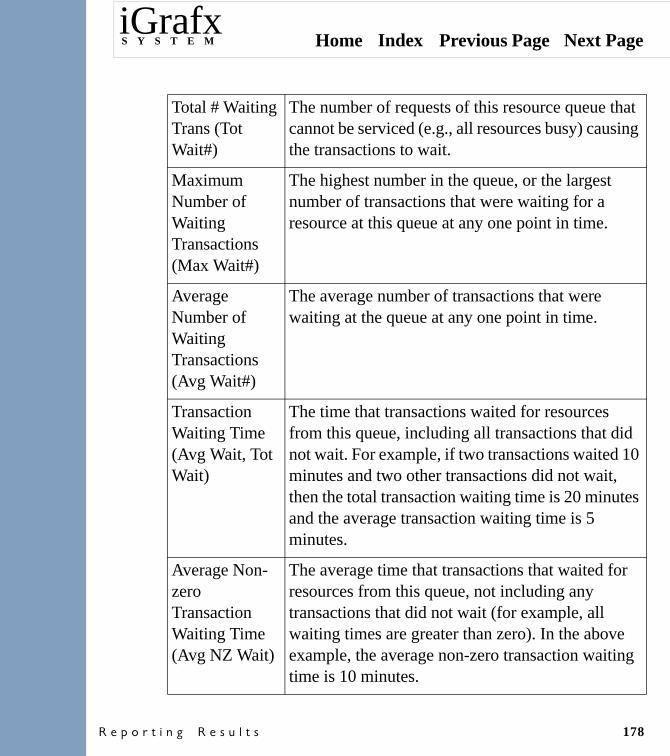
Home Index Previous Page Next PageiGrafxS Y S T E M
� � � � � � � � � � � � � � � � 178
Total # Waiting Trans (Tot Wait#)
The number of requests of this resource queue that cannot be serviced (e.g., all resources busy) causing the transactions to wait.
Maximum Number of Waiting Transactions (Max Wait#)
The highest number in the queue, or the largest number of transactions that were waiting for a resource at this queue at any one point in time.
Average Number of Waiting Transactions (Avg Wait#)
The average number of transactions that were waiting at the queue at any one point in time.
Transaction Waiting Time (Avg Wait, Tot Wait)
The time that transactions waited for resources from this queue, including all transactions that did not wait. For example, if two transactions waited 10 minutes and two other transactions did not wait, then the total transaction waiting time is 20 minutes and the average transaction waiting time is 5 minutes.
Average Non-zero Transaction Waiting Time (Avg NZ Wait)
The average time that transactions that waited for resources from this queue, not including any transactions that did not wait (for example, all waiting times are greater than zero). In the above example, the average non-zero transaction waiting time is 10 minutes.

Home Index Previous Page Next PageiGrafxS Y S T E M
� � � � � � � � � � � � � � � � 179
Creating Custom Statistics in the Report Window
You can create custom statistics to make calculations that are specific to your design, using arithmetic operators, scenario attributes, and functions.
To create custom statistics
1 With a report window active, on the ������� menu, click �����!������.
The������!����������� dialog box appears.
To modify a statistic, select it and click �����$.
To delete a statistic, select it and click �� ���.
2 To add a new statistic, click ���.
The�+���������!���������� dialog box appears.
3 For &�!�, type a brief name to describe the statistic.
4 Select ���������, ��������, +*�������, or ������.
���������. Select one of the statistics: Total Time Elapsed, Completion Count, Service Time, Waiting Time, Cycle Time, Work Time, Resource Wait Time, Blocked Time, Cost, VA Cost, BVA Cost, or NVA Cost.
For example, TotalOrders equals the number of transactions that complete.
TotalOrders = Completion Count

Home Index Previous Page Next PageiGrafxS Y S T E M
� � � � � � � � � � � � � � � � 180
��������. Select the name of the resource and one of the following: Count, Use Count, Time Busy, Time Out Of Service, Time Waiting, Total Cost, Busy Cost, Use Cost, Time Idle, and Overtime.
For example, InUse equals the time busy for resource named Laser.
InUse = Laser Time Busy
+*�������. Click to use scenario attributes, functions, members, operators, and already-defined custom statistic names to create an expression.
For example, if the wage rate is $15 per hour, then you use the following expression.
Wage = 15 * Hours(Time)
������. Select the name of the monitor and one of the following: Completion Count, Service Time, Waiting Time, Attribute Value, Cycle Time, Work Time, Resource Wait Time, Blocked Time, Cost, VA Cost, BVA Cost, or NVA Cost.
For example, Total Count equals the number of transactions that have come through a monitor.
TotalCount = Pass Count
5 For ,����, check the box to indicate that the statistic is hidden (for example, not part of the output results in the report). You can click to toggle the box.
6 After you finish editing the �����!����������� dialog box, click ��.

Home Index Previous Page Next PageiGrafxS Y S T E M
� � � � � � � � � � � � � � � � 181
Unless you have specified that it is hidden, the definition of the custom statistic is added the �����! tab on the report window.
After you create a custom statistic, you view its results by creating a report element with �����!������ as the ��������� category. The statistic can be added to any tab (for example, Time, Cost, and Resource) in the report window.
Naming or Deleting Simulation Data
You can create reports that do the following:
• Append a new report to an existing report so that you can compare the results of a subsequent simulation.
• Replace the report data with each simulation.• Create a new report for each simulation, the default setting (for
example, reports are named Sim #1, Sim #2, and so forth).The report names and creation options appear in the Run Setup dialog box and in the report elements. This dialog box appears when you select the Run Setup command on the Model menu.
To name or delete simulation data
1 On the ������ menu, click ��!� ���� ����.
The ��!� ����������dialog box appears. It contains a list of the simulation runs that are currently appended to the report. If a name is dimmed, it is unassigned.
2 Select the simulation name.

Home Index Previous Page Next PageiGrafxS Y S T E M
� � � � � � � � � � � � � � � � 182
3 Click &�!� to display the &�!����!� ����������dialog box.
4 Type a name.
5 Click �� to close the�&�!����!� ��������� dialog box.
6 Click � ��� to close the���!� ��������� dialog box.
Using Department Statistics
When activities span multiple departments, the report results take into account the shared elements of time, cost, and resources.
In the report results, a cross-department activity appears in each of the departments that participate in the activity. You use the Structure tab of the Edit Report Element dialog box to specify that individual departments appear in the row legends. For example, the department names and the text for the activity are displayed in the report element.

Home Index Previous Page Next PageiGrafxS Y S T E M
� � � � � � � � � � � � � � � � 183
Cross-Department Time Statistics
Transaction Statistics (Time)
When a transaction is processed in a cross-department activity, time accumulates in the same manner as for an activity in one department. In other words, the time that the transaction spends being processed accumulates the same for one department as for several. Like all transaction statistics, the time can be either working, waiting for resource, blocked, or inactive time. If you look at the transaction statistics by department, you will see that the time accumulates the same in each department that participates in the cross-department activity.
For example, at a Support Agency, a service bulletin (the transaction) is reviewed for one hour by editors from two departments. The transaction working time is one hour, so each department accumulates one hour of working time.
An interesting result of work being performed in parallel is that time accumulates in several departments concurrently. If you add up the working times of several departments, the sum can easily exceed the total elapsed time of the simulation. In the above example, the total service time is one hour and not two hours.

Home Index Previous Page Next PageiGrafxS Y S T E M
� � � � � � � � � � � � � � � � 184
Activity Statistics (Time)
When a transaction is processed by a cross-department activity, the activity accumulates time. Like all activity statistics, this means that the activity can be accumulating work time, resource waiting time, blocked time, or inactive time. If you look at this time sorted by department, you will see that each department accumulates the same time.
For example, at a Software Code Review meeting, participants from three departments attend a meeting that takes three hours. The activity accrues three hours in each department but the total working time is three hours and not nine hours.
Cross-Department Cost Statistics
Transaction Statistics (Cost)
Transaction costs for a cross-department activity are the result of adding or accumulating both fixed costs and resource costs. When a transaction is processed, the fixed cost of the activity is split equally among all participating departments. The resource costs are assigned to their individual departments.
Let’s begin with a simple example that uses only a fixed activity cost and no resource costs. For a bulk mailing of a brochure (the transaction), two departments share in the purchase of a mailing list that costs $400. The transaction has a total cost of $400, of which $200 is accrued in each department.

Home Index Previous Page Next PageiGrafxS Y S T E M
� � � � � � � � � � � � � � � � 185
Activity Statistics (Cost)
Each department that participates in a cross-department activity accrues activity statistics.
To continue the previous example, look at how the fixed costs are created for an activity. Fixed costs are assigned as part of the Activity Base in the Task tab on the Edit Activity dialog box (see previous page).
Now add resource costs to the previous example. The labels for the brochure (still the transaction) are printed using a computer from Dept. A and another printer from Dept. B (the two resources). Creating the labels takes one hour.
The activity still has a fixed cost of $400 to buy the mailing list. The computer in Dept. A costs $20 per hour and the printer in Dept. B costs $40 per hour.
By default, the fixed costs for a cross-department activity apply to all participating departments. However, you can use the Other resource type to model fixed activity costs that are used by individual departments.

Home Index Previous Page Next PageiGrafxS Y S T E M
� � � � � � � � � � � � � � � � 186
Cross-Department Resource Statistics
Resources
The resources associated with a cross-department activity can be used by an individual department or by all departments that participate in the activity. In other words, in the Resources tab of the Edit Activity dialog box, you can name an individual department or choose All departments. If a resource is specified for All departments, then each department uses its own instance of the resource.
For example, in a Corporate Planning Division, two departments participate in a two-hour planning meeting. The activity specifies that it uses one worker resource and one laptop computer, each of which we defined to exist in a separate pool by department. The resource specification applies to both departments, that is, each department uses one of their own workers and one of their own computers, for a total of two of each. The following are the resource definitions in the Scenario window.
The resource statistics indicate which departments used individual resources.
Home Index Previous Page Next PageiGrafxS Y S T E M
� � � � � � � � � � 187
Using Graphs
Creating Graphs
You can display report elements in either a tabular format or as a graph. If you select a graph, several graph types are available, including such common graphs as pie charts and line graphs, and other more unusual graphs such as a scatter graph or a box-whisker graph.
When you run a simulation, statistics are gathered about process times, costs, resource utilization, and queues. These statistics are categorized by transaction, activity, resource, or monitor.
You can use custom statistics to create your own unique combinations of the standard statistics. For example, you can set costing information or revenue formulas. The custom statistics are updated and calculated automatically with each simulation.
You can also maintain several sets of named simulation data to compare results across simulation runs and scenarios.
The report results can be displayed as a graph. You have your choice of 2D or 3D styles for many of the graphs.

Home Index Previous Page Next PageiGrafxS Y S T E M
� � � � � � � � � � 188
To create a graph using report data
1 In a report window, double-click the report element that you want to graph.
2 In the +�����������+ �!�� dialog box, select the ���!�� tab.
3 For ���� �$���, select �����.
This adds the ��������$ � button.
4 Click ��������$ �.
The ����������� dialog box appears. Use this dialog box to select the type of graph and other characteristics such as style, titles, fonts, markers, and background.
Graph Types
You can select different titles, fonts, and colors for many of the areas and descriptive text in a graph. The style options that are available depend on the type of graph that you select.
Pie Chart
The pie chart, one of the simplest graph types, consists of a circle (or pie) divided into two or more sections (slices). Pie charts show the proportion of parts to the whole. By labeling each pie slice with the quantity it represents, you can also compare parts to each other, although not as effectively as with a bar graph or other graph type.
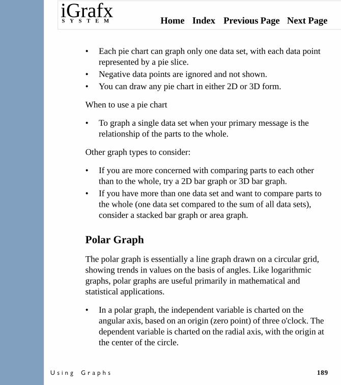
Home Index Previous Page Next PageiGrafxS Y S T E M
� � � � � � � � � � 189
• Each pie chart can graph only one data set, with each data point represented by a pie slice.
• Negative data points are ignored and not shown.• You can draw any pie chart in either 2D or 3D form.
When to use a pie chart
• To graph a single data set when your primary message is the relationship of the parts to the whole.
Other graph types to consider:
• If you are more concerned with comparing parts to each other than to the whole, try a 2D bar graph or 3D bar graph.
• If you have more than one data set and want to compare parts to the whole (one data set compared to the sum of all data sets), consider a stacked bar graph or area graph.
Polar Graph
The polar graph is essentially a line graph drawn on a circular grid, showing trends in values on the basis of angles. Like logarithmic graphs, polar graphs are useful primarily in mathematical and statistical applications.
• In a polar graph, the independent variable is charted on the angular axis, based on an origin (zero point) of three o'clock. The dependent variable is charted on the radial axis, with the origin at the center of the circle.
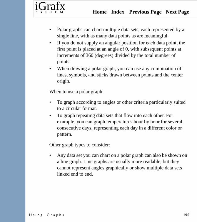
Home Index Previous Page Next PageiGrafxS Y S T E M
� � � � � � � � � � 190
• Polar graphs can chart multiple data sets, each represented by a single line, with as many data points as are meaningful.
• If you do not supply an angular position for each data point, the first point is placed at an angle of 0, with subsequent points at increments of 360 (degrees) divided by the total number of points.
• When drawing a polar graph, you can use any combination of lines, symbols, and sticks drawn between points and the center origin.
When to use a polar graph:
• To graph according to angles or other criteria particularly suited to a circular format.
• To graph repeating data sets that flow into each other. For example, you can graph temperatures hour by hour for several consecutive days, representing each day in a different color or pattern.
Other graph types to consider:
• Any data set you can chart on a polar graph can also be shown on a line graph. Line graphs are usually more readable, but they cannot represent angles graphically or show multiple data sets linked end to end.

Home Index Previous Page Next PageiGrafxS Y S T E M
� � � � � � � � � � 191
Bubble Graph
A bubble graph is a special form of the scatter graph showing bubbles, which are circular markers of variable size plotted on an X-Y grid. The size of each bubble is typically used to show the relative importance of a data point, such as the percentage of gross sales it represents. You can use a bubble graph to chart three variables in two dimensions.
• In a bubble graph, all three variables are independent. You can select which variable to show on the X axis, which to show on the Y axis, and which to show by the size of the bubble.
• You must supply values for the X position, Y position, and bubble size for each point.
• You cannot draw curves on a bubble graph.
When to use a bubble graph:
• When you have three variables to graph and want to show them on a single set of axes.
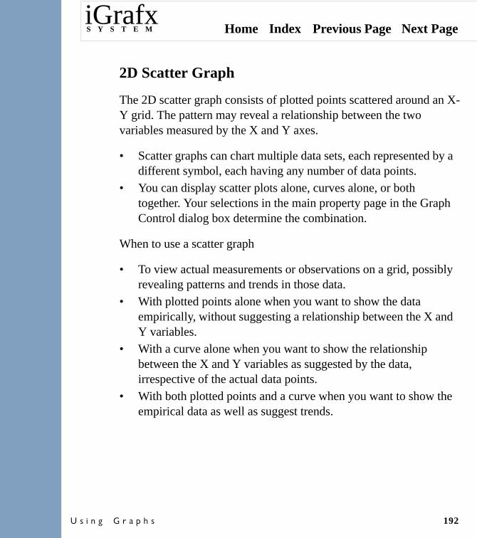
Home Index Previous Page Next PageiGrafxS Y S T E M
� � � � � � � � � � 192
2D Scatter Graph
The 2D scatter graph consists of plotted points scattered around an X-Y grid. The pattern may reveal a relationship between the two variables measured by the X and Y axes.
• Scatter graphs can chart multiple data sets, each represented by a different symbol, each having any number of data points.
• You can display scatter plots alone, curves alone, or both together. Your selections in the main property page in the Graph Control dialog box determine the combination.
When to use a scatter graph
• To view actual measurements or observations on a grid, possibly revealing patterns and trends in those data.
• With plotted points alone when you want to show the data empirically, without suggesting a relationship between the X and Y variables.
• With a curve alone when you want to show the relationship between the X and Y variables as suggested by the data, irrespective of the actual data points.
• With both plotted points and a curve when you want to show the empirical data as well as suggest trends.

Home Index Previous Page Next PageiGrafxS Y S T E M
� � � � � � � � � � 193
Other graph types to consider:
• When you are graphing against only two variables and you can plot points at regular intervals along the X axis without specifying X positions, you should generally use a line graph with symbols instead of a 2D scatter graph.
3D Scatter Graph
The 3D scatter graph consists of plotted points scattered around an X-Y-Z space. The pattern may reveal a relationship between the three variables measured by the X, Y, and Z axes.
• Scatter graphs can chart multiple data sets, each represented by a different symbol, each having any number of data points.
• When defining a scatter graph, you usually supply an X position for each data point. However, you can supply no X positions and automatically place points at X increments of 1, starting at 0.
• You can emphasize the Y value of each plotted point by selecting the Sticks option in the main property page in the Graph Control dialog box.
When to use a 3D scatter graph:
• To view actual measurements or observations in 3D space, possibly revealing patterns and trends in those data.

Home Index Previous Page Next PageiGrafxS Y S T E M
� � � � � � � � � � 194
Other graph types to consider:
• When you are graphing against three variables, consider a bubble graph, which is generally easier to read than a 3D scatter graph. Instead of using three axes (X, Y, and Z), bubble graphs plot bubbles of different sizes along an X and a Y axis. The third variable is shown by the size of each bubble.
Line Graph
The line graph consists of one or more lines (or sequences of symbols) drawn on an X-Y grid. These graphs let you show trends in values over a continuous scale.
• In a line graph, the X axis usually represents an independent variable, which is most often a time scale. The Y axis usually shows a dependent variable, such as a quantity or percentage.
• When drawing a line graph, you can use any combination of lines, symbols, and vertical sticks. You can select this combination in the main property page in the Graph Control dialog box.
• In the main property page in the Graph Control dialog box, you can select to show the X axis, Y axis, or both in a logarithmic scale – creating a lin/log, log/lin, or log/log graph.
When to use a line graph:
• To show the trend of one or more data sets over time or another continuous scale.

Home Index Previous Page Next PageiGrafxS Y S T E M
� � � � � � � � � � 195
Other graph types to consider:
• If your main focus is on the quantities at various data points rather than the trends in those quantities, consider an absolute area graph.
• If you are graphing discrete values – with data points that are based on two independent variables and that do not necessarily occur at regular intervals – use a 2D scatter graph.
• If your data points are not consecutive – for example, if you want to graph data only for 1987, 1990, and 1992 – a 2D bar graph or 3D bar graph may be more appropriate.
2D Bar Graph
A bar graph consists of two or more parallel bars of equal width drawn on an X-Y grid. Bar graphs compare amounts to each other. They can also suggest trends, especially in vertical form.
• 2D bar graphs are available in three styles: simple, stacked, and stacked percentage. You can select a style on the main property page in the Graph Control dialog box.
• You can draw bars either vertically or horizontally. In the vertical format, viewers tend to attribute a left-to-right sequence to the bars, whether you intend one or not. To select vertical or horizontal bars, go to the Style property page in the Graph Control dialog box.
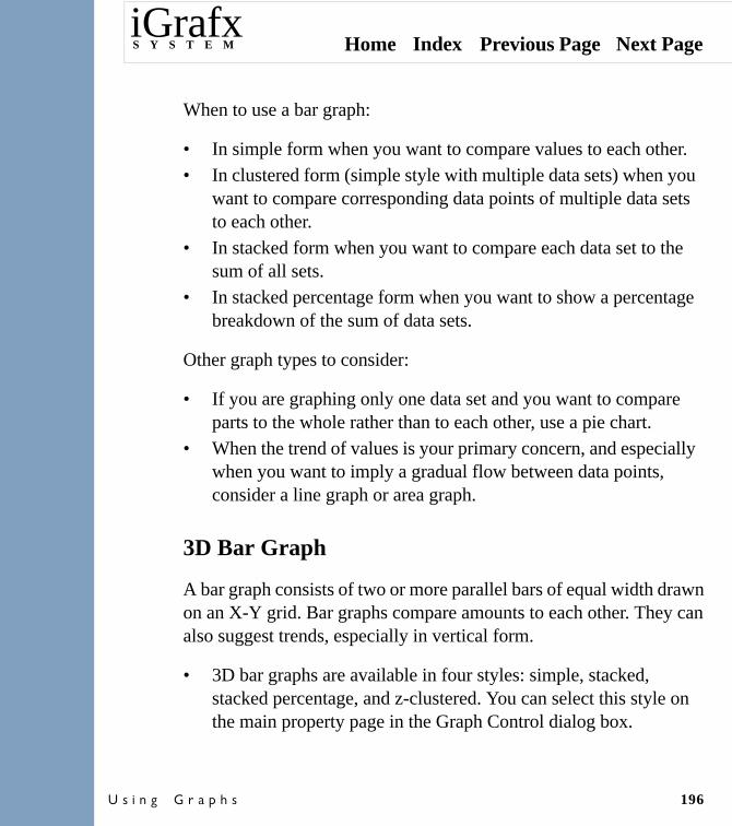
Home Index Previous Page Next PageiGrafxS Y S T E M
� � � � � � � � � � 196
When to use a bar graph:
• In simple form when you want to compare values to each other.• In clustered form (simple style with multiple data sets) when you
want to compare corresponding data points of multiple data sets to each other.
• In stacked form when you want to compare each data set to the sum of all sets.
• In stacked percentage form when you want to show a percentage breakdown of the sum of data sets.
Other graph types to consider:
• If you are graphing only one data set and you want to compare parts to the whole rather than to each other, use a pie chart.
• When the trend of values is your primary concern, and especially when you want to imply a gradual flow between data points, consider a line graph or area graph.
3D Bar Graph
A bar graph consists of two or more parallel bars of equal width drawn on an X-Y grid. Bar graphs compare amounts to each other. They can also suggest trends, especially in vertical form.
• 3D bar graphs are available in four styles: simple, stacked, stacked percentage, and z-clustered. You can select this style on the main property page in the Graph Control dialog box.

Home Index Previous Page Next PageiGrafxS Y S T E M
� � � � � � � � � � 197
• You can draw bars either vertically or horizontally. In the vertical format, viewers tend to attribute a left-to-right sequence to the bars, whether you intend one or not. To select vertical or horizontal bars, go to the main property page in the Graph Control dialog box.
When to use a bar graph:
• In simple form when you want to compare values to each other.• In clustered (simple style with multiple data sets) or z-clustered
form when you want to compare corresponding data points of multiple data sets to each other.
• In stacked form when you want to compare each data set to the sum of all sets.
• In stacked percentage form when you want to show a percentage breakdown of the sum of data sets.
Other graph types to consider:
• If you're graphing only one data set and you want to compare parts to the whole rather than to each other, use a pie chart.
• When the trend of values is your primary concern, and especially when you want to imply a gradual flow between data points, consider a line graph or area graph.

Home Index Previous Page Next PageiGrafxS Y S T E M
� � � � � � � � � � 198
Area Graph
The area graph consists of one or more lines drawn on an X-Y grid, with the area between the line and the X axis filled in. Like line graphs, area graphs show trends in values but give greater emphasis to quantities.
• Area graphs are available in three forms: stacked, absolute, and stacked percentage. You can select one of these forms on the main property page in the Graph Control dialog box.
• Negative data points are ignored and not shown.• You can draw any area graph in either 2D or 3D form.
When to use an area graph:
• To show the trend of one or more data sets over time or another continuous scale, with an emphasis on quantities.
• In cumulative form when you want to compare each data set to the sum of all sets.
• In absolute form when you want to compare data sets to each other. Absolute area graphs work better in 3D.
• In percentage form when you want to view trends in the percentage breakdown of the sum of data sets.
Other graph types to consider:
• If you want to emphasize trends themselves (the downward or upward movement of values) over quantities, use a line graph.

Home Index Previous Page Next PageiGrafxS Y S T E M
� � � � � � � � � � 199
• If you want data points to stand as separate entities rather than flowing together, consider a 2D bar graph or 3D bar graph (in stacked or stacked percentage form) rather than a cumulative or percentage area graph.
Gantt Chart
The Gantt chart is a specialized version of the horizontal bar graph in simple or stacked form. It's used almost exclusively to show a project schedule, with each bar or bar segment marking the start time, duration, and completion time of a task.
• Depending on your needs, you can have each bar represent either a single task (one solid bar) or a sequence of tasks (stacked bar).
• Gantt charts are made up of at least two data sets. The first set contains the values for the start point of each bar, and subsequent sets contain the end points of each bar segment.
• Unlike bar graphs, Gantt charts are always drawn horizontally and only in 2D form.
• Gantt bars are placed along the Y axis at increments of 1, starting at 1.
• In default form, Gantt chart bars are drawn with no spaces between them. To add spaces, go to the main property page in the Graph Control dialog box and select the Spaced option.
• You cannot show negative data points on a Gantt chart.

Home Index Previous Page Next PageiGrafxS Y S T E M
� � � � � � � � � � 200
When to use a Gantt chart:
• To graph a project schedule when you know the start time and end time for each task.
Other graph types to consider:
• If every task starts at the same point, you can use a 2D bar graph or 3D bar graph (in simple or stacked form) to show the same information.
High-Low-Close Graph
The high-low-close (HLC) graph lets you chart a range of values on an X-Y grid. The range is shown as a vertical bar, with horizontal crossbars for the high, the low, and a normative value usually called the close. An alternate version, the open-high-low-close (OHLC) graph, adds a fourth crossbar for another normative value usually called the open.
• When you click the High-Low icon on the 2D Gallery property page, you get an HLC graph by default. To get an OHLC graph, go to the main property page in the Graph Control dialog box and select the Open Values option.
• An HLC graph must have three data sets (high, low, and close values), and an OHLC graph must have four data sets (open, high, low, and close values). There is no limit on the number of data points you can graph, but each data set should have the same number.
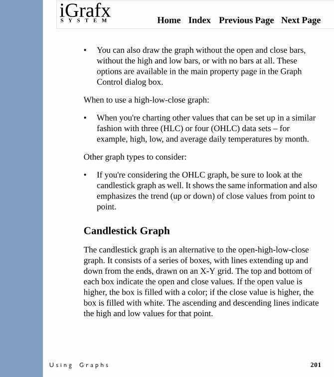
Home Index Previous Page Next PageiGrafxS Y S T E M
� � � � � � � � � � 201
• You can also draw the graph without the open and close bars, without the high and low bars, or with no bars at all. These options are available in the main property page in the Graph Control dialog box.
When to use a high-low-close graph:
• When you're charting other values that can be set up in a similar fashion with three (HLC) or four (OHLC) data sets – for example, high, low, and average daily temperatures by month.
Other graph types to consider:
• If you're considering the OHLC graph, be sure to look at the candlestick graph as well. It shows the same information and also emphasizes the trend (up or down) of close values from point to point.
Candlestick Graph
The candlestick graph is an alternative to the open-high-low-close graph. It consists of a series of boxes, with lines extending up and down from the ends, drawn on an X-Y grid. The top and bottom of each box indicate the open and close values. If the open value is higher, the box is filled with a color; if the close value is higher, the box is filled with white. The ascending and descending lines indicate the high and low values for that point.

Home Index Previous Page Next PageiGrafxS Y S T E M
� � � � � � � � � � 202
• The candlestick graph requires four data sets (open, high, low, and close values), each of which should have the same number of data points.
• If you do not supply an X position for each data point, points are placed at increments of 1, starting at 0.
• No style variants are available.
When to use a candlestick graph:
• When you're charting other values that can be set up in a similar fashion with four data sets.
Other graph types to consider:
• The open-high-low-close graph serves the same purpose as the candlestick graph, but with less emphasis on whether each plot point shows an up or down. A possible advantage of open-high-low-close over candlestick is that you can fit curves into high-low-close graphs to indicate trends in values.
Box-Whisker Graph
The box-whisker graph illustrates the spread of data groups around their medians, using a box and whiskers to break down each data group by percentile.
When creating a box-whisker graph, you can either specify the seven percentile parameters for each symbol (provide parametric data) or supply a group of raw data for the Graph Control to process and graph.

Home Index Previous Page Next PageiGrafxS Y S T E M
� � � � � � � � � � 203
• With parametric data, you need exactly seven data sets, which specify the values at percentiles of 5, 10, 25, 50 (the median), 75, 90, and 95.
• With raw data, you need enough data sets to hold all the values making up each group (always at least seven sets). When you draw the graph, sort the values for each group, then assign the seven percentile positions (5, 10, 25, 50, 75, 90, or 95) to the values closest to those percentiles. For example, in a group of 20 values, the second value would be shown as the tenth percentile.
• For raw data, you can also add symbols to the graph showing each value. If a group contains duplicate values, only one symbol is shown at that position.
• The number of data points is the number of box-whisker symbols.
When to use a box-whisker graph:
• When you want to show how the values in one or more data groups are distributed around their medians. You can either specify the percentile breakdowns of the data groups or provide raw data and have the Graph Control determine the percentile breakdowns.
Tape Graph
The tape graph is a 3D form of the line graph. It gives you only one styling option – tapes drawn between data points - but is otherwise the same as the line graph.

Home Index Previous Page Next PageiGrafxS Y S T E M
� � � � � � � � � � 204
Surface Graph
You can use the surface graph to represent data topographically in three dimensions. The graph uses an X-Z grid drawn at regular increments in the X and Z directions, with one Y value for each X-Z intersection. The color scale of the graph is automatically keyed to the height of its points, helping the viewer differentiate between higher and lower values.
• A surface graph represents a minimum of two data sets and usually at least three. Each data set holds the Y values of a row of points along the X axis. The first set applies to the row of points perpendicular to the Z origin (the back of the graph), and subsequent sets apply to additional rows.
• All panels of the surface graph (the rectangles formed by the X and Z grids) are colored according to their height. You specify the colors at the maximum and minimum points of the axis, and the Graph Control interpolates colors between these points.
• When drawing a surface graph, you can use lines to show the edges of each panel, fill each panel with a solid color, or use both lines and fills. You can also add side walls to the front and right edges of the graph. All of these options are available in the property page in the Graph Control dialog box.
Other graph types to consider:
• If your data points have irregularly spaced Z values, consider a 3D scatter graph.

Home Index Previous Page Next PageiGrafxS Y S T E M
� � � � � � � � � � 205
• If your data points have irregularly spaced X values but regular Z values, try a 3D bar graph or tape graph.

IndexiGrafxS Y S T E M
206
Home Previous Page Next Page
A
Activelimit on transactions 102
schedule times� ���
Activitybase
value base 33
capacity of 35
defining tasks� ��
definition� �
processes� ��
processingorder of processing ��
schedule� ��
setting duration� ��
statistics� ��
value base� �����
Addition, in an expression� �
Afternoon, event schedule� ���
And, logical� �
Arguments to functions� ��
Arithmetic operators� �
Attributesdefinings� �
department� ��
initializing� ���
IndexiGrafxS Y S T E M
207
Home Previous Page Next Page
locationsfinding the location of 69
number, YesNo, TrueFalse� ��
preempt� �
priority�
process� ��
scenario� ��
set before and after duration� �
setting global values� ��
transaction� ��
values during trace� ���
with split outputs� ��
Average number of waiting transactions� ���
B
Batchingby time� ���
Blocked timedelay� ��
inputs� ��
Busy time� ���

IndexiGrafxS Y S T E M
208
Home Previous Page Next Page
C
Calendar time� ���
Capacity� ��
Capacity of activity� ��
Case statement, outputs� �
Cells� ��
Changingstyles in tabular view� ��
Check model� ���
Choosinga resource� ��
Columnsviewing in tables� ��
Comparisons, in an expression� �
Composite, schedule� ���
Compressed time� ���
Concurrent subprocesses� ������
Connection lines, editing in a table� ��
Constraints, transaction flow� ��
Copyingin tabular view� ��
Costsactivity� ���
fixed, by activity� ��
in report window� ��
resources� ����������
Creating

IndexiGrafxS Y S T E M
209
Home Previous Page Next Page
a new process� ���
subprocesses� ������
Cross department activities� ��
Custom report elements� ��
Custom statistics, editing� ���
D
Data collection with monitors� ���
Dayssetting for schedule� ���
within a schedule� ���
Decision cases, outputs� �
Dedicated resources� ��
Definingattributes� ����
schedules� ���
types� ��
Delayas activity� ��
Deletingin tabular view� ��
Department attributes� ��
Departmentsand simulation� �
cross-activities� ��
Division, in an expression� �

IndexiGrafxS Y S T E M
210
Home Previous Page Next Page
Duration, on activity� ��
E
End of day, event schedule� ���
Equipmentas a resource� ��
Errors, reviewing in the output window� ���
Event� ���
Event schedule� �������
Expressionsadding attributes to� ��
adding members to� ��
using� ��
F
Familyabout transactions�
First day of the month, schedule� ���
First of month, event schedule� ���
Fixed costactivity base� ��
resource� ���

IndexiGrafxS Y S T E M
211
Home Previous Page Next Page
Functionsadding� �
defining� ��
list of� ��
mappingdistribution 96
using system� ��
G
Generatorscopying to clipboard� ���
icon in the Modeling toolbardefining 103
Graphs� ���
Groupstransaction
of inputs 17
H
Hierarchycreating� ���
viewing the process hierarchy� ���
Holidays� ���

IndexiGrafxS Y S T E M
212
Home Previous Page Next Page
Hourly rate, resource costs� ���
Hours, setting for schedule� ���
I
Idle time� ���
Inactive time, scheduling� ���
Input collectionsabout� �
Inputsdefining activity� �
groups� ��
queuing inputs� ��
start points� ��
L
Laboras a resource� ��
Last day of the month, schedule� ���
Last of month, event schedule� ���
Locations� �

IndexiGrafxS Y S T E M
213
Home Previous Page Next Page
M
Maximumnumber waiting� ���
Membersadding to expressions� ��
of functions� �
Minus button, in outline form� ���
Mod operator� �
Monitordata collection� ���
defining� ��
finding� ���
finding multiple� ���
placing� ���
symbol in tabular view� ��
Morning, event schedule� ���
Movingin tabular view� ��
Multiple Scenarios� ���
Multiplication, in an expression� �
N
Night hours� ���

IndexiGrafxS Y S T E M
214
Home Previous Page Next Page
O
Operators, adding to expressions� �
Or, logical� �
Order of processing� ��
Other resources, cost� ��
Out of serviceresource behavior� ��
resources and overtime� ��
Outline form, using� ���
Output windowchecking models� ���
Outputsdefining activitiy� ��
defining decisions� �
splitting� ��
stopping processing� ��
Overtimeactivity behavior� ��
resource behavior� ��
resource costs� ��
resources� ��
schedules� ���

IndexiGrafxS Y S T E M
215
Home Previous Page Next Page
P
Parentheses, in an expression� �
Pause during trace� ���
Percentages for outputs� �
Plus button, in outline form� ���
Pools, using resource� ���
Preempt attribute� �
Priority attribute�
Private subprocesses� ������
Processattributes� ��
creating hierarchy� ���
viewing� ���
viewing multiple in Trace window� ���
Q
Queue methodsabout� ��
Attr Member� ��
By Expression� ��
By Time� ��
Entire Family� ��
Entire Group� ��
Input Paths� ��

IndexiGrafxS Y S T E M
216
Home Previous Page Next Page
Queuesautomatically managed� �
in the report window� ��
methods to set� ��
reviewing resources in the report window� ���
Queuing inputs, minimum and maximum� ��
R
Releasing a worker if waiting� ��
Reportselements� ��
report window tabs� ��
setting run initialization options� ���
viewing in the report window� ��
Resource Assignment Type� ��
Resource Behavior� ��
Resource Costs� ���
Resource Overtime� ��
Resource Quantity� ��
Resource Schedule� ��
Resource Statistics� ���
Resourcesadding to an activity� ��
copying to clipboard� ���
costs� ���
defining� ��

IndexiGrafxS Y S T E M
217
Home Previous Page Next Page
forcing from family� ��
in the report window� ��
overtime� ��
quantity� ��
reviewing cost statistics� ��
reviewing time statistics� ���
schedules� ��
using� ��
utilization� ���
waiting time� ���
Resources Waiting� ��
ResourcesTab� ��
Resume tool� ���
Run Setupcopying to clipboard� ���
setting data� ���
snapshots� ���
S
Scenarioattributes� ��
copying and pasting� ���
data, copying to clipboard� ���
definition� ���
deleting� ���

IndexiGrafxS Y S T E M
218
Home Previous Page Next Page
openingtool on Modeling toolbar 126
opening multiple� ���
Scenario Data� ���
Scenario Window� ���
Schedulecomposite� ���
copying to clipboard� ���
defining� ���
defining days� ���
defining hours� ���
event� ���
for activity� ��
for resources� ��
overtime� ���
using� ���
Selectingin tabular view� �
Sequence for random numbers� ���
Settingpreempts on a transaction� �
priorities on transactions�
work durations� ��
Simulationsnapshots� ���
starting and stopping� ���
Simulation data� ���
IndexiGrafxS Y S T E M
219
Home Previous Page Next Page
Snapshotstaking during simulations� ���
Splittingoutputs� ��
Standard days� ���
Standard hours� ���
Start Points for process diagrams� ��
Start/Resume tool� ���
Startingovertime� ��
the simulator� ���
Statisticsabout transactions� ��
by department� ���
custom� ���
formulas� ������
resource times� ���
reviewing resource costs� ��
reviewing resource queues� ���
reviewing resource time� ���
subsets of resource busy time� ���
summary on activity� ��
transaction formulas� ��
Stop tool� ���
Stoppingprocess of outputs� ��
the simulator� ���
Styles, changing in tabular view� ��
IndexiGrafxS Y S T E M
220
Home Previous Page Next Page
Subprocesseshierarchy� ���
on an activity� ��
Subtraction, in an expression� �
Summary, comments on activity statistics� ��
Suspend overtime� ��
Swing hours� ���
Symbols, for Start� ��
System functionslist of� ��
using� ��
T
Tableschanging styles of font, fill, border, or symbol� ��
connecting symbols with lines� ��
moving, copying, and deleting cells� ��
viewing� ��
viewing columns� ��
Tabular viewchanging styles� ��
reviewing start points and monitors� ��
selecting cells� �
Task, setting duration� ��
Tilingwindowing techniques� ���

IndexiGrafxS Y S T E M
221
Home Previous Page Next Page
Timecompressed vs. calendar� ���
resource waiting� ���
reviewing resource statistics� ���
Total transaction waiting time� ���
Tracemultiple processes� ���
numbers� ���
pause� ���
starting and stopping� ���
window� ���
Transaction Statistics� ��
Transactionsactive limits� ���
attributes in subprocesses� ��
definition� �
family�
flow constraints� ��
formulas� ��
values during trace� ���
Typesdefining attributes and functions� ��
IndexiGrafxS Y S T E M
222
Home Previous Page Next Page
U
Usingexpressions� ��
resources� ��
Utilization, resource� ���
V
Value� �����
View Scenarios tool� ��
Viewingtabular� ��
W
Waiting timeinputs� ��
WaitTime� ��
Weekend days� ���
Windowsscenario window� ���
message window 111
techniques for viewing multiple processestiling 149

IndexiGrafxS Y S T E M
223
Home Previous Page Next Page
trace window, using� 130
Workercustom statistic� 172
resource� ��
wait time� 24

Micrografx End-User License Agreement
����������������������� ����������������������������������������������������������������������
�������������������������������������������������� ��������������������������������������������������������������������������������������������������������������������������������������� ������������������������������������������ ��������������������������������������������������������������� �������������������������������������������������������������������������������� ����������������������������������������������������������������������������������������������������������������
������������������������������������������������������������������������� �� ����� �����������������������������������������������������������������������������������������
1. GRANT OF LICENSE. This License is granted to you in consideration for full payment of all fees associated with the Micrografx software (hereinafter referred to as "the Software'"), in accordance with the terms defined by Micrografx, the Software dealer, or on the site allowing for the downloading of the Software. The License permits you to use one copy of the Software on any single computer If the Software is permanently installed on the hard disk or other storage device of a computer, then the person authorized to use such computer also may use the Software on a portable computer, laptop or home computer so long as the Software is not used on both computers at the same time. If such person's authorization to use such computer ceases for any reason (e.g. termination of employment), then such person's authority to use the software on a portable computer, laptop and home computer will cease. The Software is licensed as a single unit, and its component programs may not be separated for use on different computers. You must acquire and dedicate a license for each separate computer on which the Software is installed or run from the storage device. A License for the Software may not be shared or used concurrently on different computers. Installation and/or usage on a network server requires a License for every user who accesses the Software at any time.
2. OWNERSHIP. Title, ownership rights, and intellectual property rights in and to the Software will remain in Micrografx and is protected by United States copyright laws and international treaty provisions. There is no transfer to you of any title to or ownership of the Software and this License should not be construed as a sale of any right in the Software. You must treat the Software like any other copyrighted materials, except that you may either (a) make one copy of the Software solely for backup or archival purposes, or (b) transfer the Software to a single hard disk provided you keep the original solely for backup or archival purposes. You may not copy written materials accompanying the Software. You may use the Software in your own personal and business documents as long as you are not selling the output generated by the Software or any related services. You may modify the Software and/or merge it into another computer program to the extent necessary for your own use on the network or computer, but any portion of the Software merged into another computer program will continue to be subject to this License.
3. UPGRADES. If the Software is labeled as an upgrade, you must be properly licensed to use a product identified by Micrografx as being eligible for the upgrade in order to use the Software. The Software labeled an "upgrade" replaces and/or supplements the product that formed the basis for your eligibility for the upgrade. The upgrade may not be separated for use from the product, or transferred separately or used on more than one computer except as set forth above.
4. OTHER RESTRICTIONS. This License, delivered with the Software or which may be printed from the web site allowing for the downloading of the Software is your proof of license to exercise the rights granted herein and must be retained by you. You may not rent or lease the Software, but you may transfer your rights under this License on a permanent basis provided that you transfer this License, the Software and all accompanying written materials, you retain no copies, and the recipient agrees to the terms of this License. You may not translate, decompile, or disassemble the Software or make any attempt to discover the source code to the Software. If the Software is an update, any transfer must include the update and all prior versions. Further, you may not place the Software onto a server so that it is accessible via a public network such as the Internet.
5. MULTIPLE MEDIA. You may receive the Software in more than one medium. Regardless of the type or size of the medium you receive, you may use only the media appropriate for your single designated computer or network server. You may not use any other media on another computer or computer network, or loan, rent, lease, or transfer them to another user except as part of a transfer or other use expressly permitted by this License.
6. LIMITED WARRANTY. MICROGRAFX WARRANTS THAT THE SOFTWARE WILL PERFORM SUBSTANTIALLY ACCORDING TO THE WRITTEN MATERIALS DELIVERED WITH THE SOFTWARE, WHICH MAY BE PRINTED OR DOWNLOADED, FOR NINETY (90) DAYS FROM THE DATE OF ORIGINAL PURCHASE. MICROGRAFX DISCLAIMS ALL OTHER WARRANTIES, EITHER EXPRESS OR IMPLIED (INCLUDING WITHOUT LIMITATION, IMPLIED WARRANTIES OR MERCHANTABILITY AND FITNESS FOR A PARTICULAR PURPOSE) CONCERNING THIS SOFTWARE AND ITS ACCOMPANYING WRITTEN MATERIALS. Some jurisdictions do not allow limitations on duration of an implied warranty, so the above limitation may not apply to you. This limited warranty gives you specific legal rights. You may have others which vary by jurisdiction.
7. REMEDIES. Micrografx's entire liability and your exclusive remedy will be replacement of the Software by Micrografx that does not meet Micrografx's Limited Warranty. For this purpose, you shall, with respect to Software delivered on tangible media, return the Software and the written materials to Micrografx or the place from which it was purchased with a copy of your receipt; with respect to Software which may be downloaded, contact Micrografx or your dealer directly. This Limited Warranty is void if failure of the Software has resulted from accident, abuse, or misapplication. Any replacement Software will be warranted for the remainder of the original warranty period or thirty (30) days, whichever is longer.
8. LIMITATION OF LIABILITY. In no event will Micrografx or its suppliers be liable for any damages whatsoever (including, without limitation, damages for loss of business profits, business interruption, loss of business information, or other pecuniary loss) arising out of the use of or inability to use the Software, even if Micrografx has been advised of the possibility of such damages. More specifically, Micrografx will not be liable for the technical procedure for the downloading of the Software. Because some states do not allow the exclusion or limitations of consequential or incidental damages, the above limitations may not apply to you.
9. EXPORT RESTRICTIONS. You may not export or reexport the Software or any underlying information or technology except in full compliance with all United States and other applicable laws and regulations.
10. U.S. GOVERNMENT RESTRICTED RIGHTS The Software and documentation are provided with RESTRICTED RIGHTS. Use, duplication, or disclosure by the government is subject to restrictions as set forth in subparagraph (c) (1) (ii) of the Rights in Technical Data and Computer Software clause as DFARS 252.227-7013 or subparagraphs (c) (1), and (2)

of the Commercial Computer Software-Restricted Rights at 48 CFR 52.227-19, as applicable, and any amendments thereto.
11. MISCELLANEOUS PROVISIONS. This License is governed by the laws of the State of Texas, USA (and not by the 1980 United Nations Convention on Contracts for the International Sale of Goods, as amended). This is the entire agreement between us relating to the Software and supersedes any purchase order, communication, advertising, or representation concerning the Software. No change or modification of this License will be valid unless it is in writing and is signed by an authorized representative of Micrografx. If this Software was acquired outside the United States, then local law may apply. If you acquired this Software in Canada, you agree to the following:
The parties to this License have expressly required that the License be drawn up in the English language./ Les parties aux présentes ont expressement exigé que la présente convention soit rédigée en langue anglaise.
Copyright © May 2000 by Micrografx, Inc.

��������������� ������������������������������������ ������������������������������������������������������������� ������ �
��� ��������������� �� �������������������������������������� ������ ���������� ������������������������������
���������� ����������������!��"����"����#� �$����������������������������� ��� ���������� ������ �������#�������������������
�������������������������������������������������������������
��������������� ��������������������
���������������������������! #��% ������������������&������'������(��)���������*+�,#��-�������������������+����������������
-��������������������'������&����.���������.�����.��������/�����0��)!���&����*+�1����*+�������1����-����1����������1����&��������
�� (������������������ ��� ����)�����������������
!��#��������%����������������+�������+���&������'� ��'�����'����&���������������������������)����������������������������)�
�&/��������&������������������������ ������������������������������� ������������������1��������������(����������������������
+����2�������3�$�����)��������.������4�� ���.��������������.������(��)���0��)1������&� �&����&����4������'������5.���&�� ����
6����)��������������������� ��� ����)������ ����)�����������������
.���������������������� ��2�3������ ��%�����-��,������+����%�����7�� ��������7��������#���899:%������!��"����"����#� �
+����%�����7�� ��������7��������#������� ����)���%�����-��,������
���!����������899;<899=�������������
!���������������899=�������������
!�����������������899><899?'����������,��!��������!6&!�!��"����"����#� �
(�� "#��'��������������������899><899=�!��"����"����#� �
%�������������������899=���������������������!��"����"����#� �
���������������������899;���������������������!��"����"����#� �
+�����@�����������@�.���������7��� ����&� ��7���������899:<899=+����������������!��"����"����#� �
�����&�����7'������-��������������8998<899?���������������!��"����"����#� �
(��.�������(A�� ���������899;<899=������������������
4��������4�������!������4�������!�����4�������4������4��������������4���������������4�������������4��������������4�������
��������4������������/� ������4������������%����4�������/��� ��4�������/AB�� ������4�������&�������+�����B��������������� �/�
+��� ���$��=�.��#�����&�����&����C�����-�������><�<8D����+��@.�����&����������+��@�����+��@.-"�4�������-���&������4�������&��� ����
4�������-���$�#��������������������� ��� ����)������ ����)���4������������������ ����)-�������������� ��4�������������(���'�������
-������� ���6��� E�� ����%��������.�����&������,� �
6"(�6"(���!����)�����,����&�����$�����6"(!��F���6"('�����)�6"(E�����6"(!����!��F���6"(,�����6"(��������6"(.���� ��
$����&����$����"�����$������������������������ ��� ����)������ ����)���6"(6��������������������!��"����"����#� �
��������@+����G@&�������+�#��������E�2&+E3��������������� ��� ����)����� ����)������������������������6��� &������� D�������
���������
+����G@�� �&�������+�#��������E��� +����G@�� ����������899�<899?�������������������
.���������������899><899;1�������������������
1��"�� ���899?<8999!�����&����)�����!��"����"����#� �
�������������������&���������������������������899*���$&/�����������!��"����"����#� �
�������������������&��������� ����)���$&/�����������
/������� ����������� ������ ����)����������� ��� ����)��������������#����������