IFS DOCUMENTATION PART II: DATA ASSIMILATION (CY25R1) · 2015-11-12 · 7 ‘Background, analysis...
129
IFS Documentation Cycle CY25r1 1 IFS Documentationn Cycle CY25r1 (Edited 2003) IFS DOCUMENTATION PART II: DATA ASSIMILATION (CY25R1) (Operational implementation 9 April 2002) Edited by Peter W. White (Text written and updated by members of the ECMWF Research Department) Table of contents Chapter 1 ‘Incremental formulation of 3D/4D variational assimilation—an overview’ Chapter 2 ‘3D variational assimilation’ Chapter 3 ‘4D variational assimilation’ Chapter 4 ‘Background term’ Chapter 5 ‘Conventional observational constraints’ Chapter 6 ‘Satellite observational constraints’ Chapter 7 ‘Background, analysis and forecast errors’ Chapter 8 ‘Gravity-wave control’ Chapter 9 ‘Data partitioning (OBSORT)’ Chapter 10 ‘Observation screening’ Chapter 11 ‘Analysis of snow’ Chapter 12 ‘Land surface analysis’ Chapter 13 ‘Sea surface temperature and sea-ice analysis’ Chapter 14 ‘Reduced-rank Kalman filter’ REFERENCES
Transcript of IFS DOCUMENTATION PART II: DATA ASSIMILATION (CY25R1) · 2015-11-12 · 7 ‘Background, analysis...
IFS Documentation Cycle CY25r1
ent)
IFS DOCUMENTATION
PART II: D ATA ASSIMILATION (CY25R1)(Operational implementation 9 April 2002)
Edited by Peter W. White
(Text written and updated by members of the ECMWF Research Departm
Table of contents
Chapter 1 ‘Incremental formulation of 3D/4D variational assimilation—an overview’
Chapter 2 ‘3D variational assimilation’
Chapter 3 ‘4D variational assimilation’
Chapter 4 ‘Background term’
Chapter 5 ‘Conventional observational constraints’
Chapter 6 ‘Satellite observational constraints’
Chapter 7 ‘Background, analysis and forecast errors’
Chapter 8 ‘Gravity-wave control’
Chapter 9 ‘Data partitioning (OBSORT)’
Chapter 10 ‘Observation screening’
Chapter 11 ‘Analysis of snow’
Chapter 12 ‘Land surface analysis’
Chapter 13 ‘Sea surface temperature and sea-ice analysis’
Chapter 14 ‘Reduced-rank Kalman filter’
REFERENCES
1
IFS Documentationn Cycle CY25r1 (Edited 2003)

Part II: ‘Data Assimilation (CY25R1)’
e Eu-
her than
in this
ecasts
Copyright
© ECMWF, 2003.
All information, text, and electronic images contained within this document are the intellectual property of th
ropean Centre for Medium-Range Weather Forecasts and may not be reproduced or used in any way (ot
for personal use) without permission. Any user of any information, text, or electronic images contained with
document accepts all responsibility for the use. In particular, no claims of accuracy or precision of the for
will be made which is inappropriate to their scientific basis.
2
IFS Documentation Cycle CY25r1 (Edited 2003)
IFS Documentation Cycle CY25r1
t of the
lation,
d pre-
dients
Var
nd
de-
nd
eed-
d in
re de-
i-
e chief-
system
Part II: D ATA ASSIMILATION
CHAPTER 1 Incremental formulation of 3D/4Dvariational assimilation—an overview
Table of contents
1.1 Introduction
1.2 Incremental Formulation
1.3 Practical implementation
1.3.1 Data flow
1.3.2 Formation of high-resolution analysis
1.3.3 Humidity and ozone
1.4 Preconditioning and control variable
1.5 Minimization
1.1 INTRODUCTION
This documentation on 3D and 4D–Var is meant to serve as a scientific guide to the 3D/4D–Var codes, a par
IFS. The documentation is divided into eleven chapters. This, the first chapter deals with the scientific formu
the practical implementation of the incremental method, and it includes some comments on minimization an
conditioning. The code structure and the computational details of the 3D/4D-Var cost-functions and their gra
are explained inChapter 2 ‘3D variational assimilation’. There is a separate chapter on subjects specific to 4D-
(Chapter 3 ‘4D variational assimilation’). Thereafter follows a description of the background term (Chapter 4
‘Background term’) and two chapters respectively on observation operators for conventional data (Chapter 5 ‘Con-
ventional observational constraints’) and satellite data (Chapter 6 ‘Satellite observational constraints’). Chapter
7 ‘Background, analysis and forecast errors’deals with the computation of background and analysis errors a
Chapter 8 ‘Gravity-wave control’is on initialization. The modules for observation sorting and screening are
scribed inChapter 9 ‘Data partitioning (OBSORT)’andChapter 10 ‘Observation screening’. Chapter 11outlines
the snow analysis,Chapter 12describes the Soil analysis,Chapter 13describes the sea surface temperature a
sea-ice analysis and the final chapterChapter 14 provides details of the reduced Kalman filter.
An extensive scientific description of 3D/4D-Var has been published in QJRMS, in ECMWF workshop proc
ings and Technical Memoranda over the years. The incremental formulation was introduced byCourtier et al.
(1994). The ECMWF implementation of 3D-Var was published in a three-part paper byCourtieret al.(1998),Ra-
bier et al. (1998) andAnderssonet al. (1998). The observation operators for conventional data can be foun
Vasiljevicet al.(1992). The methods for assimilation of TOVS radiance data and ERS scatterometer data we
veloped byAnderssonet al. (1994) andStoffelenand Anderson(1997), respectively. The pre-operational exper
mentation with 4D-Var has been documented in three papers byRabieret al. (1998),Mahfouf and Rabier(1998)
andKlinker et al. (1999).
3D-Var was implemented in ECMWF operations on 30 January 1996. The three-part paper mentioned abov
ly presented the scheme as it was at that point in time. There have been very significant developments of the
1
IFS Documentationn Cycle CY25r1 (Edited 2003)
Part II: ‘Data assimilation’
stem
ere re-
er-
s intro-
(sim-
was
instead
,
lly
model
A con-
time
revious
ntrols
in
erator
during its time in operations. The first upgrade took place in connection with the move from a CRAY C90 sy
to a distributed memory Fujitsu VPP700 machine. The observation handling and data screening modules w
placed with new codes, seeChapter 9 ‘Data partitioning (OBSORT)’andChapter 10 ‘Observation screening’,
respectively, and the paper byJärvinenand Undén(1997). Variational quality control of observations (Andersson
and Järvinen, 1999, andSection 2.6) and a new algorithm for computing estimates of analysis and background
rors (Fisher and Courtier 1995, andChapter 7 ‘Background, analysis and forecast errors’ ) were introduced.
In May 1997 there was a complete revision of the background term, seeDerber andBouttier(1999) andChapter
4 ‘Background term’. The old background term, which was described inCourtier et al. (1998), is not covered by
this documentation as it is now considered obsolete. Later that year (25 November 1997) 6-hour 4D-Var wa
duced operationally, at resolution T213L31, with two iterations of the outer loop: the first with 50 iterations
plified physics) and the second with 20 iterations (with tangent-linear physics). In April 1998 the resolution
changed to TL319 and in June 1998 we revised the radiosonde/pilot usage (significant levels, temperature
of geopotential) and we started using time-sequnces of data (Järvinenet al.1999), so-called 4D-screening. Finally
the data assimilation scheme was extended higher into the atmosphere on 10 March 1999, when the TL319L50
model was introduced, which in turn enabled the introduction in May 1999 of ATOVS radiance data (McNaet
al. 1999). In October 1999 the vertical resolution of the boundary layer was enhanced taking the number of
levels to a total of 60. In summer 2000 the 4D-Var period was extended from 6 to 12 hours, whereas the ER
figuration was built as an FGAT (first guess at the appropriate time) of 3D-Var with a period of 6 hours. At the
of writing it is planned to increase the horizontal resolution of 4D-Var to TL511L60, with inner loop resolution
enhanced from T63L60 to TL159L60 using the linearized semi-Lagrangian scheme.
1.2 INCREMENTAL FORMULATION
3D/4D–Var attempt to minimize an objective function consisting of three terms:
(1.1)
measuring, respectively, the discrepancy with the background (a short-range forecast started from the p
analysis), , with the observations, and with the slow character of the atmosphere, . The -term co
the amplitude of fast waves in the analysis and is described inChapter 8 ‘Gravity-wave control’. It is omitted from
the subsequent derivations in this section.
In its incremental formulation (Courtieret al. 1994), we write
(1.2)
is the increment and at the minimum the resulting analysis increment is added to the background
order to provide the analysis :
(1.3)
is the covariance matrix of background error while is the innovation vector,
(1.4)
where is the observation vector. is a suitable low-resolution linear approximation of the observation op
J
J Jb Jo Jc+ +=
Jb Jo Jc Jc
J δx( ) 12---δxTB 1– δx
12--- Hδx d–( )TR 1– Hδx d–( )+=
δx δxa xb
xa
xa xb δxa+=
B d
d yo Hxb–=
yo H
2
IFS Documentation Cycle CY25r1 (Edited 2003)

Chapter 1 ‘Incremental formulation of 3D/4D variational assimilation—an overview’
n of
erator
iating
-
as
lar ma-
ervation
-
istics
ithmic
nce on
ame as
nt job
ation
ase)
main
rpose
nts,
rved
is re-
with
in the vicinity of , and is the covariance matrix of observation errors. Alternatively, inEq. (1.2)can
be replaced by the finite difference , approximated at low resolution. The incremental formulatio
3D/4D-Var consists therefore of solving for the inverse problem defined by the (direct) observation op
, given the innovation vector and the background constraint. The gradient of is obtained by different
Eq. (1.2) with respect to ,
(1.5)
At the minimum, the gradient of the objective function vanishes, thus fromEq. (1.5)we obtain the classical result
that minimizing the objective function defined byEq. (1.2)is a way of computing the following equivalent matrix
vector products:
(1.6)
where and are positive definite, see e.g.Lorenc(1986) for this standard result. may be interpreted
the square matrix of the covariances of background errors in observation space while is the rectangu
trix of the covariances between the background errors in model space and the background errors in obs
space.
Most (if not all) implementations of OI rely on a statistical model for describing and (Hollingsworth
and Lönnberg, 1986;Lönnbergand Hollingsworth, 1986 andBartelloand Mitchell, 1992). 3D-Var uses the obser
vation operator explicitly and, as OI, if a statistical model is required it is only used for describing the stat
of the background errors in model space. Consequently, in 3D/4D-Var it turns out to be easier, from an algor
point of view, to make use of observations such as TOVS radiances, which have a quite complex depende
the basic analysis variables.
1.3 PRACTICAL IMPLEMENTATION
As mentioned earlier inSection 1.2, the formulation used is incremental (Courtier et al. 1994). In the ECMWF
implementaion two different resolutions are used—one for the comparison with observations, which is the s
the deterministic medium-range forecast model, and a lower resolution for the minimization. Several differe
steps are performed:
(i) Comparison of the observations with the background at high resolution to compute the innov
vectorsEq. (1.4). These are stored in the NCMIFC1-word of the ODB (the observation datab
for later use in the minimization. This job step also performsscreening(i.e. blacklisting, thinning
and quality control against the background) of observations (seeChapter 10 ‘Observation
screening’). The screening determines which observations will be passed for use in the
minimisation. Very large volumes of data are present during the screening run only, for the pu
of data monitoring,
(ii) First minimization at low resolution to produce preliminary low-resolution analysis increme
using simplified physics
(iii) Update of the high-resolution trajectory to take non-linear effects partly into account. Obse
departures from this new atmospheric state are stored in the ODB and the analysis problem
linearized around the updated model state,
(iv) Second main minimization at low resolution with tangent-linear physics,
(v) Formation of the high-resolution analysis (described below) and a comparison of the analysis
all observations (also those not used by the analysis, for diagnostic purposes).
H xb R HδxHx Hxb–
δxH d J
δx
J B 1– HTR 1– H+( )δx HTR 1– d–=∇
δxa B 1– HTR 1– H+( ) 1– HTR 1– d BHT HBH T R+( ) 1– d= =
B R HBH T
BHT
HBH T BHT
H
3
IFS Documentation Cycle CY25r1 (Edited 2003)
Part II: ‘Data assimilation’
g,
lds to
-
ects.
,
solu-
eftra-
gsfc
hich
fc and
ds), re-
s in the
ctory
-
ctory
d to the
s great-
o
(vi) Computation of analysis and background errors, currently at T42L60, as described inChapter 7
‘Background, analysis and forecast errors’
Each of the job steps is carried out by a different configuration of IFS. They are commonly called:
(i) The first trajectory run (which includes screening and is sometimes calledthe screening run) –
conf=2, LSCREEN=.T.
(ii) The main minimization, simplified physics, conf=131, LSPHLC=.T.,
(iii) The trajectory update, conf=1, LOBS=.T.,
(iv) The main minimization with physics, conf=131, LSPHLC=.F.,
(v) The final trajectory runs , conf=1, LOBS=.T., NUPTRA=NRESUPD, with verification screenin
(vi) The background error minimization, conf=131, LAVCGL=.T.
A truncation operator (the IFS full-pos post-processing package) allows one to go from high-resolution fie
low resolution, using appropriate grid-point interpolations. The steps(iii) and(iv) are referred to as the second it
eration of theouter loop,and these can optionally be iterated further to incorporate additional nonlinear eff
The trajectory update is not normally done in 3D-Var. Theinner looptakes place within the main minimization
job steps(iii) and (v).
1.3.1 Data flow
All files containing model fields are coded in GRIB (the GRIB format is described in GRIB.ps). The high-re
tion background (the input to the first trajectory run) is obtained from a standard MARS retrieve to files r
jshml (model-level spectral fields), reftrajggml (model-level grid-point fields, i.e. and clouds) and reftrajg
(surface grid-point fields).
The is truncated to the resolution of the minimization to form (the low-resolution background), w
is the input to the main minimization. The low resolution file names are backgroundshml, backgroundggs
backgroundggml, for upper-air spectral data, surface grid-point data, and upper-air grid-point data (i.e. clou
spectively. Specific humidity and ozone are represented in spectral space as they are spectral variable
variational analysis. The three files are linked to the namesICMRFxxxx0000, ICMSHxxxxINIT and ICMG-GxxxxIMIN , ICMGGxxxxINIT, ICMGGxxxxINIUA (wherexxxx is the ‘expver’ identifier of MARS) and read
in by SUSPEC, SUGRIDF from SUECGES.
The main minimization job writes out the low-resolution background (the previous high-resolution traje
in the second minimization) to filesMXVA00000+000hhmm(where hhmm is the time of the field) and the low
resolution analysis to filesMXVA00999+00hhmm. This is done in a call toSTEPOnear the end ofSIM4D,
Section 2.3, by the routineWRMLPP. Both these files are are saved under names starting respectively withspfglrandspanlr and later read by IFS in the trajectory runs (usingSUINIF, called fromRDFPINC) and transformed to
the higher resolution by filling with zeroes (operator ), and is transformed to gridpoint space. The traje
runs also read in (from thereftraj files) usingSUINIF called fromCSTA. The analysis increment is formed
in RDFPIN:
(1.7)
1.3.2 Formation of high-resolution analysis
The analysis field is the sum of the background and of the pseudo-inverse of the truncation operator applie
low-resolution analysis and background. This pseudo-inverse comprises filling in the spectral wave-number
er than the minimization resolution by zeroes ( , applied inEq. (1.7)). At this stage temperature is converted t
virtual temperature, as required by the model. (note that normal-mode initialization is no longer applied).
xHRb
q
xHRb xLR
b
q
xLRb
xLRa
T 1– qxHR
b
δxHRa T 1– xLR
a[ ] T 1– NNMI xLRb( )[ ]–=
T 1–
4
IFS Documentation Cycle CY25r1 (Edited 2003)
Chapter 1 ‘Incremental formulation of 3D/4D variational assimilation—an overview’
IM).
antity.
) grid-
val-
er
idity.
onvert-
pplied
As the
e
mple-
r by a
, it was
of de-
e
on al-
t.
the ar-
ap-
rting
ber of
only
e cost
rom
1.3.3 Humidity and ozone
The humidity control variable used in the minimization is specific humidity in spectral space (LSPQ, NAMD
There is no constraint forcing the minimization to produce positive and non supersaturated values for this qu
However, before the computation of TOVS observation departures in the minimization stage, (low-resolution
point values are replaced by where is a differentiable function such that it results in positive humidity
ues (routineQNEGLIM, called fromTOVCLR). Super–saturated humidity gridpoint values can optionally, und
the switch LNEGHYP (=.false., namrinc), be modified to be below 1.2 (hard coded) in terms of relative hum
This would be done in the routineQNEGHYP, called fromSCAN2MDM.
The high resolution analysis of in gridpoint space, is modified (inSUGPQLIMDM, called byRDFPINC) by
resetting negative humidities to zero and supersaturated values to saturated values.
The ozone control variable used in the minimization is ozone in spectral space (LSPO3). The increment is c
ed to gridpoint space when computing the high resolution analysis. For the time being no special security is a
to the ozone increments.
1.4 PRECONDITIONING AND CONTROL VARIABLE
In practice, it is necessary to precondition the minimization problem in order to obtain a quick convergence.
Hessian (the second derivative) of the objective function is not accessible,Lorenc(1988) suggested the use of th
Hessian of the background term . The Hessian of is the matrix . Such a preconditioning may be i
mented either by a change of metric (i.e. a modified innner product) in the space of the control variable, o
change of control variable. As the minimization algorithms have generally to evaluate several inner products
found more efficient to implement a change of variable (underCHAVAR, CHAVARIN etc). Algebraically, this
requires the introduction of a variable such that
(1.8)
ComparingEq. (1.2)andEq. (1.8)shows that satisfies the requirement. thus becomes thecontrol
variableof the preconditioned problem. This is indeed what has been implemented, as will be explained inSection
4.2. A single-observation analysis with such preconditioning converges in one iteration.
1.5 MINIMIZATION
The minimization problem involved in this 3D/4D-Var can be considered as large-scale, since the number
grees of freedom in the control variable is of the order of 106. An efficient descent algorithm was provided by th
Institut de Recherche en Informatique et Automatique (INRIA, France). It is a variable-storage quasi-Newt
gorithm (M1QN3, auxlib) described inGilbert and Lemaréchal(1989) and in an on-line postscript documen
M1QN3uses the available in-core memory to update an approximation of the Hessian of the cost function (
ray ZVATRA, seeCVA1). In practice, ten updates (NMUPD, namiomi) of this Hessian matrix are used. The
proximation is modified during the minimization by deleting information from the oldest gradient and inse
information from the most recent one. Once per iterationM1QN3calls thesimulator SIM4D (Section 2.3). Some-
times extra simulations have to be performed in order to obtain a good step length for the descent. The num
iterations is limited to 70 (NITER, namvar) and the number of simulations to 80 (NSIMU, namvar). Normally,
very small adjustments of the analysis occur during the second half of the minimization. On the whole, th
function is typically divided by a factor of two and the norm of the gradient by a factor of twenty (printed f
f q( ) f
q
Jb Jb B
χ
Jb χTχ=
χ B 1 2/– δx= χ
5
IFS Documentation Cycle CY25r1 (Edited 2003)

Part II: ‘Data assimilation’
sec-
EVCOSTandSIM4D, respectively).
The approximation of the Hessian computed during a 3D/4D-Var minimization (read in bySUHESS) is used as a
first estimate for a subsequent analysis, if the switch LWARM=.true. (namiomi). LWARM is only used in the
ond minimization of 4D-Var (seeSection 3.3).
6
IFS Documentation Cycle CY25r1 (Edited 2003)
IFS Documentation Cycle CY25r1
f
ed
e com-
outines
Part II: D ATA ASSIMILATION
CHAPTER 2 3D variational assimilation
Table of contents
2.1 Introduction
2.2 Top-level controls
2.2.1 Gradient test
2.2.2 Iterative solution
2.2.3 Last simulation
2.3 A simulation
2.3.1 Interface between control variable and model arrays
2.4 Interpolation to observation points
2.4.1 Method
2.4.2 Storage in GOM-arrays
2.5 Computation of the observation cost function
2.5.1 Organization in observation sets
2.5.2 Cost function
2.5.3 Jo tables
2.5.4 Correlation of observation error
2.6 Variational quality control
2.6.1 Description of the method
2.6.2 Implementation
2.6.3 Correlated data
2.1 INTRODUCTION
This part of the documentation covers the top level controls of 3D-Var (CVA1) and gives a detailed description o
a 3D-Var simulation (SIM4D) All of this chapter also applies to 4D-Var with some additions which will be detail
in Chapter 3 ‘4D variational assimilation’. The interpolation of model fields to observation points (OBSHOR) and
the organization of the data in memory (yomsp, yommvo) are also descibed. We explain the structure of th
putation of the observation cost function (FJO and FJOS in yomcosjo1) and its gradient, managed by the r
OBSV andTASKOB. The background term will be explained inChapter 4 ‘Background term’ .
7
IFS Documentationn Cycle CY25r1 (Edited 2003)
Part II: ‘Data assimilation’
g-
e
d
utine
nction
w
terval
well
n state
d by
string
2.2 TOP-LEVEL CONTROLS
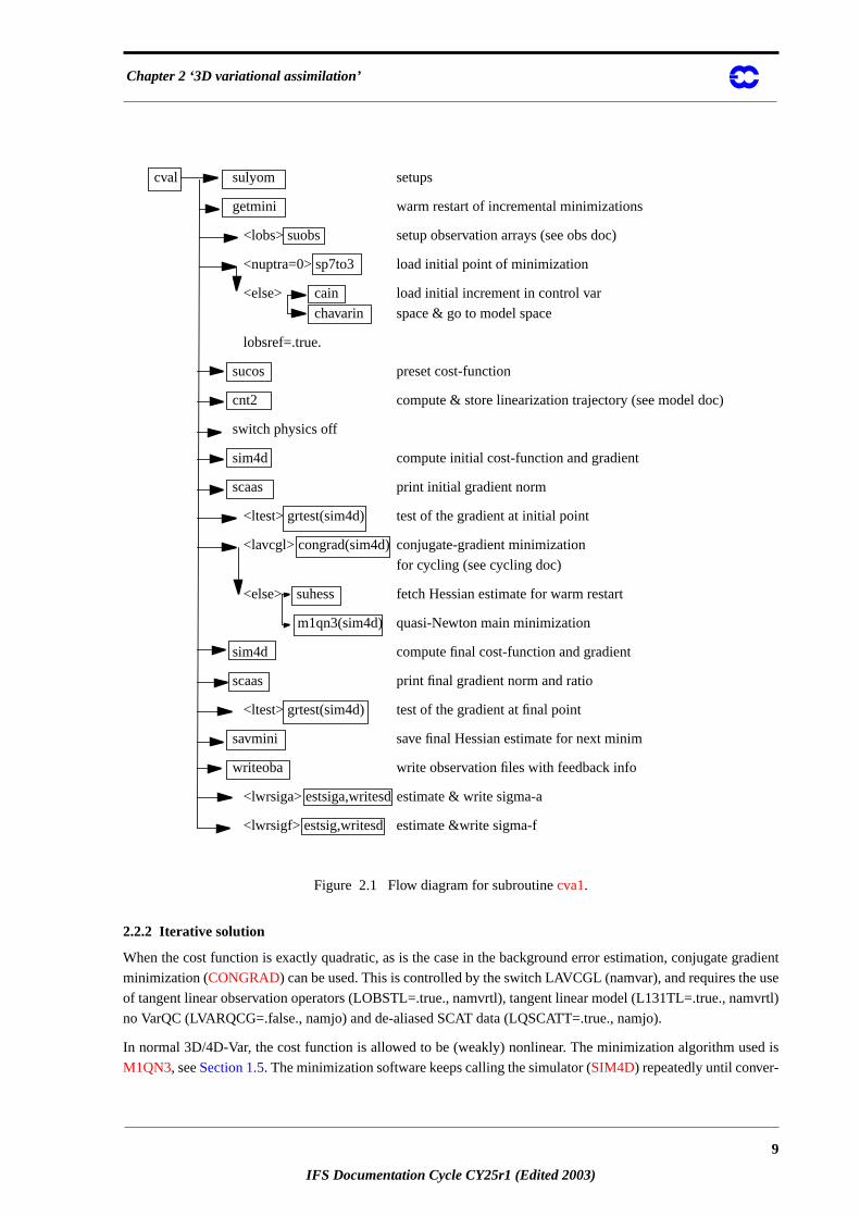
The routineCVA1 controls the variational configuration of IFS—its flow diagram is shown inFig. 2.1 . The first
guess fields (FG) have been read in to the SP7-arrays (inYOMSP) by SUECGES, called fromSUJBSTDwithin
the setup, seeSubsection 4.3.3. The FG is optionally initialized to be consistent with the lower resolution oro
raphy. This is done in a call toCNMI from SUECGES, controlled by the switch LFGNMI (=false if L50 or L60,
in namjg), see alsoChapter 8 ‘Gravity-wave control’ .
At the start ofCVA1 additional setups for the variational configurations are done (SU1YOM). The SP3-arrays, i.e.
the current model state, (inYOMSP) are filled by copying from SP7, usingSP7TO3. A call to CNT2 computes
, which is required for the finite-difference version ofEq. (1.4)of the incremental 3D-Var. This call toCNT2
is charaterized by LOBSREF=.true. (inYOMCT0). The result, stored in the NCMIFC2-word of the ODB, is th
low-resolution departurefrom the FG, , and will be used in later iterations,Eq. (2.5). If, however, the
tangent linear observation operators are used,Eq. (2.6), is not needed. It can optionally be compute
and stored, if LCALCFC2=.true. (in yomrinc).
2.2.1 Gradient test
If LTEST=.true. a gradient test will be performed both before and after minimization. This is done by the ro
GRTEST. In the gradient test a test value is computed as the ratio between a perturbation of the co-t-fu
and its first order Taylor expansion:
(2.1)
with . Repeatedly increasing by one order of magnitude, printing at each step should sho
approaching one, by one order of magnitude at a time, provided is approximately quadratic over the in
. The near linear increase in the number of 9’s in the print of over a wide range of (initially as
as after minimization) proves that the coded adjoint is the proper adjoint for the linearization around the give
.
The behaviour of the cost function in the vicinity of in the direction of the gradient is also diagnose
several additional quantities for each . The results are printed out on lines in the log-file starting with the
‘GRTEST:’. To test the continuity of , for example, a test value is computed:
(2.2)
and printed. For explanation of other printed quantities see the routineGRTEST itself.
Jb
HxLRb
yo H– xLRb
yo H– xLRb
t1
t1J χ δχ+( ) J χ( )–
J∇ χδ,⟨ ⟩--------------------------------------------
δχ 0→lim=
δχ α– J∇= α t1 t1
J χ( )χ χ δχ+[ , ] t1 α
χ
χ ∇JαJ t0
t0J χ δχ+( )
J χ( )------------------------- 1–=
8
IFS Documentation Cycle CY25r1 (Edited 2003)
Chapter 2 ‘3D variational assimilation’
radient
use
vrtl)
d is
Figure 2.1 Flow diagram for subroutinecva1.
2.2.2 Iterative solution
When the cost function is exactly quadratic, as is the case in the background error estimation, conjugate g
minimization (CONGRAD) can be used. This is controlled by the switch LAVCGL (namvar), and requires the
of tangent linear observation operators (LOBSTL=.true., namvrtl), tangent linear model (L131TL=.true., nam
no VarQC (LVARQCG=.false., namjo) and de-aliased SCAT data (LQSCATT=.true., namjo).
In normal 3D/4D-Var, the cost function is allowed to be (weakly) nonlinear. The minimization algorithm use
M1QN3, seeSection 1.5. The minimization software keeps calling the simulator (SIM4D) repeatedly until conver-
cval sulyom setups
getmini warm restart of incremental minimizations
<lobs> suobs setup observation arrays (see obs doc)
<nuptra=0> sp7to3 load initial point of minimization
<else> cain load initial increment in control var
chavarin space & go to model space
lobsref=.true.
sucos preset cost-function
cnt2 compute & store linearization trajectory (see model doc)
switch physics off
sim4d compute initial cost-function and gradient
scaas print initial gradient norm
<ltest> grtest(sim4d) test of the gradient at initial point
<lavcgl> congrad(sim4d) conjugate-gradient minimization
for cycling (see cycling doc)
<else> suhess fetch Hessian estimate for warm restart
m1qn3(sim4d) quasi-Newton main minimization
sim4d compute final cost-function and gradient
scaas print final gradient norm and ratio
<ltest> grtest(sim4d) test of the gradient at final point
savmini save final Hessian estimate for next minim
writeoba write observation files with feedback info
<lwrsiga> estsiga,writesd estimate & write sigma-a
<lwrsigf> estsig,writesd estimate &write sigma-f
9
IFS Documentation Cycle CY25r1 (Edited 2003)

Part II: ‘Data assimilation’
conver-
utput
nd
arture
ally
’
gence has been reached, or until the maximum number of iterations or simulations has been reached. The
gence criterion is given as a reduction in the norm of the gradient by a factor , in namvar. The o
mode ofM1QN3 is printed in the log-file. The interpretation is:
1) Convergence reached, according to the above criterion.
2) M1QN3 called incorrectly.
3) Line search failed—step too big, > .
4) Maximum number of iterations (NITER) reached
5) Maximum number of simulations (NSIMU) reached
6) Line search failed—step too small, < RDX, (in namvar).
7) Impossible gradient value, ‘descent’ direction points uphill.
2.2.3 Last simulation
After M1QN3 has returned control toCVA1, one final simulation is performed. This simulation is diagnostic, a
characterized by the simulation counter being set to 999, NSIM4D=NSIM4DL, yomvar. The observation dep
from the low-resolution analysis, , is computed and stored in the NCMIOMN-word of the ODB. Fin
at the end ofCVA1, the updated ODB is written to disk, using the routineWRITEOBA.
2.3 A SIMULATION
A simulation consists of the computation of and . This is the task of the routineSIM4D, seeFig. 2.2 for the
flow diagram. The input is the latest value of the control variable in the array VAZX, computed byM1QN3, or
CONGRAD. First and its gradient are computed (seeSections 1.4 and4.2):
(2.3)
The gradient of with respect to the control variable is stored in the array VAZG (YOMCVA).
• Copy from VAZX to SP3-arrays (YOMSP) using the routineYOMCAIN
• Compute , the physical model variables, usingCHAVARIN:
. (2.4)
• Perform the direct integration of the model (if 4D-Var), using the routineCNT3, and compare with
observations. SeeSection 2.5.
Calculate for whichOBSV is the master routine.
• Perform the adjoint model integration (if 4D-Var) usingCNT3AD, and observation operators
adjoint.
Calculate , and store it in SP3.
• and its gradient are calculated inCOSJCcalled fromCNT3AD, if LJC is switched on (default)
in namvar.
• Transform to control variable space by applyingCHAVARINAD .
• Copy from SP3 and add to , already in the array VAZG, usingYOMCAIN
• Add the various contributions to the cost function together, inEVCOST, and print to log file using
prtjo.
• Increase the simulation counter NSIM4D by one.
10 NCVGE–
1 20×10
yo H– xLRa
J J∇χ
Jb
Jb χTχ=
Jb 2χ=χ∇
Jb
χx
x δx xb+ Lχ xb+= =
Jo
Jox∇Jc
Jox∇ Jcx∇+
Joχ∇ Jcχ∇+ Jbχ∇
10
IFS Documentation Cycle CY25r1 (Edited 2003)
Chapter 2 ‘3D variational assimilation’
so on
hould
A3D
, set
-
ce.
riable.
The new and are passed to the minimization algorithm to calculate the of the next iteration, and
until convergence (or the maximum number of iterations) has been reached.
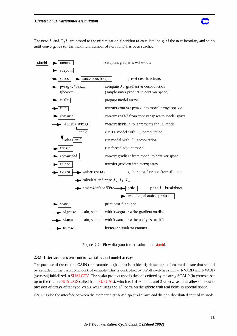
Figure 2.2 Flow diagram for the subroutinesim4d.
2.3.1 Interface between control variable and model arrays
The purpose of the routine CAIN (the canonical injection) is to identify those parts of the model state that s
be included in the variational control variable. This is controlled by on/off switches such as NVA2D and NV
(yomcva) initialized inSUALCTV. The scalar product used is the one defined by the array SCALP (in yomcva
up in the routineSCALJGScalled fromSUSCAL), which is 1 if , and 2 otherwise. This allows the com
pression of arrays of the type VAZX while using the norm on the sphere with real fields in spectral spa
CAIN is also the interface between the memory distributed spectral arrays and the non-distributed control va
J Jχ∇ χ
sim4d monvar setup an/gradients write-outs
su2yom
sucos suic,sucosjb,sujo preset cost-functions
pvazg=2*pvazx compute gradient & cost-function
fjbcost= . . . (simple inner product in cont.var space)
suallt prepare model arrays
cain transfer cont.var pvazx into model arrays spa3/2
chavarin convert spa3/2 from cont.var space to model space
<l131tl> subfgs convert fields in to increments for TL model
cnt3tl run TL model with computation
<else> cnt3 run model with computation
cnt3ad run forced adjoint model
chavarinad convert gradient from model to cont.var space
cainad transfer gradient into pvazg array
evcost gathercost I/O gather cost-function from all PEs
calculate and print
<nsim4d=0 or 999> prtio print breakdown
readoba , obatabs , prtdpst
scaas print cost-functions
<igrats> cain, stepo with ltwegra : write gradient on disk
<ianats> cain, stepo with ltwana : write analysis on disk
nsim4d++ increase simulator counter
Jb
Jo
Jo
Jc Jb Jo, ,
Jo
m 0=
L2
11
IFS Documentation Cycle CY25r1 (Edited 2003)

Part II: ‘Data assimilation’
alled
i-
sing the
cribed
ept
01 in
by the
bi-
time
gra-
ients is
The distributed spectral arrays SP3/2 are gathered with the routineGATHERSPAto form the control vector on
each processor.
2.4 INTERPOLATION TO OBSERVATION POINTS
2.4.1 Method
COBSLAGis the master routine for the horizontal interpolation of model data to observation points. It is c
after the inverse spectral transform inSCAN2MDM, and after the so-calledsemi-Lagrangian buffershave been
prepared byCOBSandSLCOMM, see the flow diagram inFig. 2.3. The interpolation code is shared with the sem
Lagrangian advection scheme of the dynamics. The buffers contain ahalo of gridpoints big enough to enable in-
terpolation to all observations within the grid-point domain belonging to the processor.COBSLAGcallsOBSHOR
which:
• Performs the interpolation, usingSLINT
• Message-passes the result to the processors where the corresponding observations belong, u
routineMPOBSEQ.
• Copies the model data at observation points to the so-called GOM-arrays (yommvo, des
below), in the routineINSOBSEQ.
There are three methods of horizontal interpolation:
1) LAIDDI : 12-point bi-cubic interpolation, used for all upper-air fields (if NOBSHOR=203) exc
clouds,
2) LAIDLI : Bi-linear interpolation, used for surface fields, and
3) LAIDLIC : Nearest gridpoint, used for cloud parameters.
The interpolation method for the upper-air fields can be switched to bi-linear by specifying NOBSHOR=2
namobs. The default is NOBSHOR=203 (bi-cubic). Lists of interpolation points and weights are prepared
routineLASCAW. In 4D-Var bi-cubic interpolation is used at high resolution (i.e. in the trajectory runs), and
linear is used at low resolution (i.e. in the main minimization). The interpolation is invoked once per 4D-Var
slot.
The adjoint (OBSHORAD) follows the same general pattern but gets further complicated by the fact that the
dient from several observations may contribute to the gradient at a given gridpoint. The summation of grad
to done in the same order, irrespective of the number of processors, as reproducibility is desired.
12
IFS Documentation Cycle CY25r1 (Edited 2003)

Chapter 2 ‘3D variational assimilation’
Figure 2.3 Flow diagram for subroutinesscan2mdm andobsv.
stepo (. . . .) scan2m buffer initializations
cobs setup field pointers
sc2rdg read grid-point data
load grid-point arrays
extmerb grid
extpolb extrapolation
cobslag scan observation arrays
obshor fetch observation lat/lon
slint horiz interpolation
to obs point
(see semilag doc)
mpobseq exchange data
among PEs
insobsec load YOMMVO
arrays GOMx
obsv reset ZFJO cost function
suobarea setup area index for each obs
(mainly according to satellite ID)
ecset define obs sets
sort TOVS/SATEM data
taskob decide whether to call TL/AD obs operators
preset ZFJO cost function
sufaceo (TL/AD) surface obs vertical operator
upperair (TL/AD) upper-air obs vertical operator
satem (TL/AD) SATEM / SSM/I obs vertical operator
tovclr (TL/AD) TOVS radiance obs vertical operator
sum cost-function for each area (diagnostic only)
sum ZFJO into FJO cost-function
<lprtgom> prtgom debugging printout of yommvo common
Jo
13
IFS Documentation Cycle CY25r1 (Edited 2003)
Part II: ‘Data assimilation’
bles
),
(skin
skin
data
ded as
are not
election
ough
/Q/
ces.
ation
erators
at case,
n
ting
ts, 2)
the
is de-
ans that
specific
-
a first
tly set
2.4.2 Storage in GOM-arrays
The GOM arrays (YOMMVO) contain the model values at observation points. The list of upper-air model varia
to appear in the GOM-arrays is under user control. There are five categories of GOM-arrays:
• GOMx for conventional data, containing full model profiles of optionally , , , , (ozon
(cloud liquid water), (clod ice) and (cloud cover)
• GOSx for conventional data, containing surface data of (surface pressure),
temperature). (soil water content), (snow cover), (roughness length) and (
reservoir water content).
• GSMx for TOVS data, containing full model profiles similar to GOMx
• GSSx for TOVS data, containing surface data of , , , , , , and , where
and are lowest model level wind components.
• GSCx for SCAT data, containing lowest model level data of , , , and , and surface
of and . (roughness length) is to be added shortly.
The reason for this split is purely to save space in memory. Model profiles of wind for example are not nee
inputs to the TOVS and SATEM operators, so those fields are not interpolated to the TOVS locations, and
stored, unless requested. Upper-air profiles of model data at SCAT locations are also not computed. The s
of model variables to interpolate to GOMx and GSMX arrays, respectively, is flexible and is controlled thr
namelist switches LGOMx and LGSMx (in namdim). The default is that only LGOM-U/V/T/Q and LGSM-T
O3 are ON, with the addition of LGSMCLW/CLI/CC in screening run to enable computation of cloudy radian
The adressing of the GOM-arrays is done by referring to the MAPOMM (YOMOBA) and MABNOB (YOMOB-
SET) tables, e.g. ZPS(jobs) = GOSP(MAPOMM(iabnob)), where iabnob = MABNOB(jobs,kset) is an observ
counter local to each processor.
The trajectory GOM5 arrays (identical to GOM) are allocated in the case that tangent linear observation op
are used. They are to hold the trajectory interpolated to the observation locations, and the GOM-arrays, in th
hold the perturbations.
At the end of the adjoint observation operators the GOM-arrays are zeroed and overwritten by the gradient (iPRE-
INTAD).
The r.m.s. of the GOM arrays is printed (byPRTGOM) if the switch LPRTGOM=.true., (inYOMOBS). The de-
fault is that the print is switched on. It can be located in the log file by searching for ‘RMS OF GOM’. The prin
is done fromOBSV, 1) when the GOM arrays contain the background interpolated to the observation poin
when it contains of the first simulation, 3) when it contains first TL perturpations after the initial call to
minimizer and 4) when it contains at the final simulation.
2.5 COMPUTATION OF THE OBSERVATION COST FUNCTION
The cost function computation follows the same pattern for all observational data. This common structure
scribed in the following section. It is assumed that all observations are independent of each other, which me
the cost function contribution from each observation station can be computed independently of others. The
observation operators for all data types and variables is detailed inChapter 5 ‘Conventional observational con
straints’ andChapter 6 ‘Satellite observational constraints’ .
2.5.1 Organization in observation sets
The vertical observation operators are vectorized over NMXLEN (yomdimo) data. To achieve this the dat
have to be sorted by type and subdivided into sets of lengths not exceeding that number. NMXLEN is curren
u v T q O3
CLW CLI CCpsurf Tskin
ws sn z0 wl
ps Ts ws sn z0 wl ul vl ul
vl
ul vl Tl ql
ps Ts z0
J∇ o
J∇ o
14
IFS Documentation Cycle CY25r1 (Edited 2003)

Chapter 2 ‘3D variational assimilation’
n op-
ntegra-
n
ich for
deals
n in
ng
he
ed
cific to
rvation
tum is
for
o data
able
nt of
an
tines
lution
to 511, inSUDIMO. The observation sets may span several 4D-Var time slots, as the input to the observatio
erators is the GOM-arrays which have been pre-prepared for all time slots during the tangent linear model i
tion. The organization of the sets is done inECSETandSMTOV and the information about the sets is kept i
yomobset. The only reason to have a separate routine for TOVS data (SMTOV) is that the TOVS sets must not
contain data from more than one satellite. This is controlled by sorting according to the area-parameter, wh
TOVS data is an indicator of satellite ID, prior to forming the sets. The area-parameter is determined inSUOBA-
REA, and is irrelevant for the observation processing for all data other than TOVS.
2.5.2 Cost function
The master routine controlling the calls to the individual observation operators is called HOP. This routine
with all different types of observations.
The HOP/HOPTL/HOPAD routines are called fromTASKOB/TASKOBTL/TASKOBAD (called fromOBSV/
OBSVTL/OBSVAD) in a loop over observation sets. The data type of each set is know from the informatio
tables such as MTYPOB(KSET) stored in yomobset.
The following describesHOP/HOPTL. The adjointHOPAD follows the reverse order.
• First prepare for vertical interpolation using the routinePREINT. Data on model levels are
extracted from the GOM-arrays (YOMMVO). Pressures of model levels are computed usi
GPPRE. Help arrays for the vertical interpolation are obtained (PPINIT) and * and are
computed (CTSTAR). * and are later used for extrapolation of temperature below t
model’s orography,Subsection 5.3.2. The routine PREINTS deals with model surface fields need
for the near-surface observation operators and PREINTR deals with those fields that are spe
the radiance observation operators.
• The observation array is then searched to see what data is there. The ‘body’ of each obse
report is scanned for data, and the vertical coordinate and the variable-number for each da
retained in tables (ZVERTP and IVNMRQ). These tables will later constitute the ‘request’
model equivalents to be computed by the various observation operators. Tables of pointers t
(‘body’ start addresses) and counters are stored (arrays IPOS and ICMBDY).
• Then the forward calculations are performed. There is an outer loop over all known ‘vari
numbers’. If there are any matching ocurrences of the loop-variable number with the conte
IVNMRQ, then the relevant observation operator will be called. A variable-number and
observation operator are linked by a table set up in the routine HVNMTLT. The interface rou
PPOBSA (upperair) andPPOBSAS(surface) are used, which in turn callPPFLEV and the
individual operator routines. For radiance data the interface isRADTR which calls the radiative
transfer code (Subsection 6.4.1).
• In HDEPART, calculate the departure as
, (2.5)
where the two terms in brackets have been computed previously: the first one in the high reso
trajectory run (Section 1.3) and the second one in the LOBSREF call, described inSection 2.2.
If LOBSTL then is
, (2.6)
which simplifies to what has been presented inSection 1.2.
T T0
T T0
z
z yo Hx– yo HxHRb–( ) yo HxLR
b–( )–+=
z
z yo Hδx– yo HxHRb–( ) yo–+=
15
IFS Documentation Cycle CY25r1 (Edited 2003)
Part II: ‘Data assimilation’
timate
the
inds
ts of
unt,
adjoint
d quan-
d in
int
s used
l
lute ob-
an be
nces of
ATEM
n 21r2,
The TOVS radiance bias correction is also carried out at this point by subtracting the bias es
(kept in the NCMTORB-word of ODB) from the calculated departure.
Finally the departure is divided by the observation error (NCMFOE in ODB) to form
normalized departure.
• Departures of correlated data are multiplied by , see2.5.4. The division by has already
taken place inHDEPART, so at this point is in fact a correlation (not a covariance) matrix.
• The cost function is computed inHJO, as
(2.7)
for all data except SCAT data. The SCAT cost function combines the two ambiguous w
(subscripts 1 and 2) in the following way (also inHJO)
(2.8)
These expressions for the cost function are modified by variational quality control, seeSection 2.6.
The cost-function values are store in two tables, as detailed in2.5.3.
• HJOalso stores the resultingeffective departurein the NCMIOM0-word of ODB, for reuse as the
input to the adjoint. The effective departure is the normalized departure after the effec
observation error correlation and quality control have been taken into acco
, where the QC-weight will be defined below,Section 2.6.
2.5.2 (a) Adjoint. We have now reached the end of the forward operators. In the adjoint routineHOPADsome
of the tasks listed above have to be repeated before the actual adjoint calculations can begin. The input to the
(the effective departure) is read from the ODB. The expression for the gradient (with respect to the observe
tity) is then simply
(2.9)
which is calculated inHOPADfor all data. The gradient of is much more complicated and is calculate
a separate section ofHOPAD. The adjoint code closely follows the structure of the direct code, with the adjo
operators applied in the reverse order.
2.5.3 Jo tables
There are two different tables for storing the values. One is purely diagnostic (FJO, yomcosjo1), and i
for producing the printed tables in the log-file (PRTJOcalled romEVCOST). The other (FJOS) is the actua
-table. FJO is indexed by observation type, sub-obstype, variable and area. FJOS is indexed by the abso
servation number, iabnob=MABNOB(jobs,kset), so that the contributions from each individual observation c
summed up in a predetermined order (inEVCOST), to ensure reproducibility.
2.5.4 Correlation of observation error
The observation error is assumed uncorrelated (i.e. the matrix is diagonal) for all data except time-seque
SYNOP/DRIBU surface pressure and height data (used by default in 4D-Var,Järvinen et al.1999). There is also
code for vertical correlation of observation error for radiosonde geopotential data (not used by default) and S
thicknesses (not used by default). IN FACT, all vertcal correlations of observation error have been removed i
σo
R 1– σo
R
Jo zTz=
JSCAT
J14J2
4
J14 J2
4+-------------------
1 4⁄=
zeff zTR 1– QCweight[ ]=
Jo 2zeff σo⁄–=obs∇
JSCAT
Jo
Jo
Jo
R
16
IFS Documentation Cycle CY25r1 (Edited 2003)
Chapter 2 ‘3D variational assimilation’
ction
corre-
ans-
action
rs.
tions
titu-
cost
weight
bly re-
C is a
ecause
e, an
nction
h are
con-
ssume
and one
but will be reintroduced again in a later cycle!
The serial correlation for SYNOP and DRIBU data is modelled by a continuous correlation function
where =RTCPART=0.3 and =RTCEFT=6.0 hours, under the switch LTC (namjo). The remaining fra
of the error variance is assumed uncorrelated (seeCOMTC).
The radiosonde geopotential data are vertically correlated (under the switch LRSVCZ) using a continuous
lation function where =RRSZPART=0.8, a tuning constant close to 1 and and are tr
formation values, based on a sixth degree polynomial in of the two pressures involved. The remaining fr
of the variance is assumed uncorrelated (seeCOMATP).
The vertical correlation of SATEM thickness data is as described inKelly and Pailleux(1988) and is assigned in
SURAD(and kept inYOMTVRAD). There is no horizontal correlation of SATEM and TOVS observation erro
The inter-channel correlation of radiance observation error is also assumed to be zero.
When is non-diagonal, the ‘effective departure’ is calculated by solving the linear system of equa
for , using NAG routines F07FDF (Choleski decomposition) and F07FEF (backwards subs
tion), as is done in UPPERAIR,SATEM, COMTC andJOPDF. The NAG routines will shortly be replaced by the
corresponding LAPACK routines SPOTRF and SPOTRS.
2.6 VARIATIONAL QUALITY CONTROL
The variational quality control, VarQC, has been described byAndersson and Järvinen(1999). It is a quality con-
trol mechanism which is incorporated within the variational analysis itself. A modification of the observation
function to take into account the non-Gaussian nature of gross errors, has the effect of reducing the analysis
given to data with large departures from the current iterand (or preliminary analysis). Data are not irrevoca
jected, but can regain influence on the analysis during later iterations if supported by surrounding data. VarQ
type of buddy check, in that it rejects those data that have not been fitted by the preliminary analysis, often b
it conflicts with surrounding data.
2.6.1 Description of the method
The method is based on Bayesian formalism. First, ana priori estimate of the probability of gross error is
assigned to each datum, based on study of historical data. Then, at each iteration of the variational schema
posterioriestimate of the probability of gross error is calculated (Inglebyand Lorenc, 1993), given the cur-
rent value of the iterand (the preliminary analysis). VarQC modifies the gradient (of the observation cost fu
with respect to the observed quantity) by the factor (the QC-weight),which means that data whic
almost certainly wrong ( ) are given near-zero weight in the analysis. Data with a are
sidered ‘rejected’ and are flagged accordingly, for the purpose of diagnostics and feedback statistics, etc.
The normal definition of a cost function is
(2.10)
where is the probability density function. Instead of the normal assumption of Gaussian statistics, we a
that the error distribution can be modelled as a sum of two parts: one Gaussian, representing correct data
flat distribution, representing data with gross errors. We write:
(2.11)
ae b t1 t2–( )2–
a b1 a–
ae b x1 x2–( )2– a b x1 x2
pln
1 a–
R zeff
zeffR z= zeff
P G( )i
P G( )f
1 P G( )f–
P G( )f 1≈ P G( )f 0.75>
Jo pln–=
p
pi Ni 1 P Gi( )–[ ] FiP Gi( )+=
17
IFS Documentation Cycle CY25r1 (Edited 2003)
Part II: ‘Data assimilation’
ctively:
r-
ormal
QC,
ssible
ithout
ng of
rvation
. Var-
where subscript refers to observation numer . and are the Gaussian and the flat distributions, respe
(2.12)
(2.13)
The flat distribution is defined over an interval which inEq. (2.13)has been written as a multiple of the obse
vation error standard deviation . SubstitutingEqs. (2.11)to (2.13)into Eq. (2.10), we obtain after rearranging
the terms, an expression for the QC-modified cost function and its gradient , in terms of the n
cost function
: (2.14)
(2.15)
(2.16)
where
(2.17)
2.6.2 Implementation
Thea priori information i.e. and are set during the screening, in the routineDEPART, and stored in the
NCMFGC1 and NCMFGC2-words of the ODB. Default values are set inDEFRUN, and can be modified by the
namelist namjo. VarQC can be switched on/off for each observation type and variable individually using LVAR
or it can be switched off all together by setting the global switch LVARQCG=.false. Since an as good as po
‘preliminary analysis’ is needed before VarQC starts, it is necessary to perform part of the minimization w
VarQC, and then switch it on. This is controlled by NITERQC in yomcosjo, and is set to 40 by default. Printi
VarQC results is done by the routinePRTQC.
JOCOST computes according toEq. (2.15) and the QC-weight—the factor within brackets inEq. (2.16).
2.6.3 Correlated data
The quality control of radiosonde height data (if used) is more complex because of the correlation of obse
error (seeJOPDF). This is one of the reason why we changed to using temperature data instead, from cy18r6
QC for correlated data is no longer supported.
i i N F
Ni1
2πσo
----------------- 12---
yi Hx–
σo-------------------
2
–exp=
Fi1Li----- 1
2liσo-------------= =
Li
σo
JoQC J∇ o
QC
JoN
JoN 1
2---
yi Hx–
σo-------------------
2
=
JoQC
γ i J– oN[ ]exp+
γ i 1+------------------------------------
ln–=
JoQC∇ Jo
N 1γ i
γ i JoN–[ ]exp+
------------------------------------– ∇=
γ iP Gi( ) 2li( )⁄
1 P Gi( )–[ ] 2π⁄--------------------------------------------=
P G( )i li
JoQC
18
IFS Documentation Cycle CY25r1 (Edited 2003)
IFS Documentation Cycle CY25r1
in
mation
ed), it
low
nitial
-
ed in
Part II: D ATA ASSIMILATION
CHAPTER 3 4D variational assimilation
Table of contents
3.1. Introduction
3.2. Organization of data in time slots
3.2.1 Observation preprocessing.
3.2.2 Inside IFS.
3.2.3 Observation screening in 4D-Var
3.3. Inner and outer loops: practical implementation
3.4. Tangent linear physics
3.4.1 Set-up
3.4.2 Mixed-phase thermodynamics
3.4.3 Vertical diffusion
3.4.4 Sub-grid scale orographic effects
3.4.5 Large-scale precipitation
3.4.6 Long-wave radiation
3.4.7 Deep moist convection
3.4.8 Trajectory management
3.1 INTRODUCTION
4D-Var is a temporal extension of 3D-Var. Observations are organized in one-hour time-slots as describedSec-
tion 3.2. The cost-function now measures the distance between a model trajectory and the available infor
(background, observations) over an assimilation interval or window. For a 12-hour window (as currently us
is either (03UTC–15UTC) or (15UTC–03UTC).Eq. (1.2)(seeChapter 1 ‘Incremental formulation of 3D/4D var-
iational assimilation—an overview’ is replaced by
(3.1)
with subscripti the time index. Eachi corresponds to one-hour time slot. is as before the increment at
resolution at initial time, and the increment evolved according to the tangent linear model from the i
time to time indexi. and are the covariance matrices of observation errors at time indexi and of background
errors respectively. is a suitable linear approximation at time indexi of the observation operator . The inno
vation vector is given at each time step by , where is the background propagat
J δx( ) 12---δxTB 1– δx
12--- Hiδx ti( ) di–( )T
i 0=
n
∑ Ri1– Hiδx ti( ) di–( )+=
δxδx ti( )
Ri BHi Hi
di yio Hixb ti( )–= xb ti( )
19
IFS Documentationn Cycle CY25r1 (Edited 2003)
Part II: ‘Data assimilation’
r-
s
ts, a
r and
lems
tion.
the
e
ber of
outer
within
loops
s with
ics on
iza-
d time
then
e to the
and soil
are
time using the full nonlinear model and is the observation vector at time indexi. As SYNOP and DRIBU time
sequences of surface pressure and height data are now usedwith serial correlation of observation error, the obse
vation costfunction computation for those data spans all time slots.Eq. (3.1)therefore needs generalising, as ha
been done in the paper byJärvinen et al. (1999).
The minimization is performed in the same way as in 3D-Var. However, it works fully in terms of incremen
configuration which is activated by the switches L131Tl and LOBSTL, and involves running the tangent-linea
adjoint models iteratively as explained inSection 2.3of Chapter 2 ‘3D variational assimilation’, and using the tan-
gent-linear observation operators.
A way to account in the final 4D-Var analysis for some non-linearities is to define a series of minimization prob
(3.2)
with superscriptn the minimization index.
is the current estimate of the atmospheric flow. It is equal to the background for the first minimiza
is the innovation vector, computed by integrating the model at high resolution from
current estimate. The way the increment is added to the current estimate is similar to that used in 3D-Var (seChap-
ter 1 ‘Incremental formulation of 3D/4D variational assimilation—an overview’ .
(3.3)
The number of times the trajectory is updated, i.e. the number of outer-loops (which corresponds to the num
minimizations performed), is typically a number between one and four. In operational 4D-Var the number of
loops is two.
This can be controlled in the prepIFS set-up, together with the number of inner-loops (iterations of m1qn3)
each minimization. One outer-loop corresponds to what is normally done in 3D-Var. The number of inner-
should then be 70 as in 3D-Var. The most standard 4D-Var uses two outer-loops. The first minimization run
the simplified physics on 50 inner-loops. The second minimization runs with the more complete linear phys
25 inner-loops. Switches for the two sets of physics will be given inSection 3.4.
The variational quality-control (Chapter 2 ‘3D variational assimilation’ Section 2.6) is switched on at the default
iteration number (40) in the first minimization. It is activated from the first iteration in the subsequent minim
tions.
The final 4D-Var trajectory is post-processed every 3 hours. Fields called 4v are created with initial date an
the start of the window (03UTC or 15UTC) and steps every 3 hours. The 4v field valid at 12UTC or 00UTC, is
renamed as the final analysis (type=an) for the atmospheric fields and the waves. The cycling from one cycl
next is performed by taking these analysis fields, together with the surface fields updated by the SST, snow
moisture analyses as input to a 12-hour forecast which produces the background for the next cycle.
The analysis and forecast error calculations are performed as explained inChapter 7 ‘Background, analysis and
forecast errors’, with the inclusion of the time dimension in the minimization. The analysis error variances
available at the beginning of each window, and the forecast error variances at the end.
yio
J δxn( ) 12--- δxn xn 1– xb–+( )TB 1– δxn xn 1– xb–+( )=
12--- Hiδxn ti( ) di
n 1––( )T
i 0=
n
∑ Ri1– Hiδxn ti( ) di
n 1––( )+
xn 1–
din 1– yi
o Hixn 1– ti( )–=
xHRn xHR
n 1– NNMI xHRn 1– δxHR
n+( ) NNMI xHRn 1–( )–+=
20
IFS Documentation Cycle CY25r1 (Edited 2003)
Chapter 3 ‘4D variational assimilation’
OC
d on
r more
roc-
ithin
tter of
riods,
melist/
each
e, the
length
n having
f anal-
ta, se-
us, the
rvation
tine
report
N-
-
KEC-
outine
re
y also
e sub-
ristics
med
tine
ed in
3.2 ORGANIZATION OF DATA IN TIME SLOTS
3.2.1 Observation preprocessing.
Observational input data (BUFR-format) is read in by means of 6-hour time-windows in OBSPR
preproc_mpp_makecma. Before input, each time-window has been organised into several BUFR-files base
major observation types. Input BUFR-files are labelled and split so that every processor can read one o
BUFR-files. The prefix of each file indicates the observation type. The suffix “<tw>.<proc>” defines which p
essor <proc> (here within a range [1..16]) will be responsible for inputting data for time-window <tw> (here w
a range [01..02]). The number of files is not necessarily equal to the number of processors, it is really a ma
I/O-load balancing, and the end result is independent of the reading order.
In the case of 4D-Var there are NO6HTSL input time-windows. For 6 h, 12 h and 24 h 4D-Var analysis pe
the NO6HTSL will have values 1, 2 and 4, respectively. This can be set via the namelist namelist/namglp.h (see
also yomglp).
Another affecting parameter (see discussion about reshuffle below) is NOSORTSL (set via OBSPROC na
nammkcma.h and declared in yommkcma). It defines how many time-slots will be used. The rule is to divide
input time-window into 1h out time-slots, but with half an hour lengths for start and end time-slots. Therefor
value of NOSORTSL should be set to 7, 13 or 25 for 6 h, 12 h and 24 h 4D-Var analysis periods (i.e. one plus
of a 4D-Var period in hours), respectively.
Once all BUFR-data has been successfully read in, the unique sequence numbers for reports (before eve
them around!) are generated in OBSORT-routinemakeseqno_obsortcalled bypreproc_mpp_makecma. These
numbers are always independent of the number of processors in use. They form a basis for reproducibility o
ysis results regardless of how many processors were used.
The sequence numbers are generated without honouring the input time-windows. Currently for CONV-da
quence numbers start at offset 0, TOVS at offset 1,000,000, SCAT at 2,000,000 and SSMI 3,000,000. Th
increment is set to 1,000,000 meaning that we may not exceed more than one million reports per major obse
type (CONV, TOVS, etc.) without making a small change into the local variable increment in rou
preproc_mpp_makecma.
After the sequence-number generation, all BUFR data is read in and re-shuffled for better load balancing in
creation under the OBSPROC-routine MAKECMAmakecma. Before that, the number of input time-windows
NO6HTSL has already been reset to one inpreproc_mpp_makecma, and all 4D-Var BUFR input data is regarded
as a one ‘supertime-window’ for initial report creation. However, via NAMELIST parameters NANTIM, NA
DAT, NTBMAR and NTFMAR defined in NAMGLP (namelist/namglp.h and yomglp), full control over valid 4D
Var analysis timerange is maintained. Therefore, observations not in this range will be discarded by the MA
MA.
An essential step to organise observational data for 4D-Var purposes occurs in the OBSPROC r
postproc_mpp_makecma. The aim is to reshuffle and time-slot the initially created CMA files of which there a
currently one CMA file per processor. The CMA data needs not only to be organised in time-slots, but the
need to obtain a better geographical distribution within a given time-slot to have a better load balancing in th
sequent IFS/Screening job.
Before the reshuffle of observations can take place, some crucial information about 4D-Var run characte
needs to be passed on. Parameters NANTIM, NANDAT, NOSORTSL, NTBMAR and NTFMAR are transfor
into the suitable constants for use by the OBSORT by use of SETPARAM_OBSORT in rou
postproc_mpp_makecma. The following conversion takes place (OBSORT parameters in concern are declar
21
IFS Documentation Cycle CY25r1 (Edited 2003)
Part II: ‘Data assimilation’
riod.
d
nd
o
f the
t
pshot in-
report
tly the
proc-
ssed by
ted by
e, so
e sub-
ith its
OB-
ndow
ed not
ed by
ack
.The
yomstdin):
• NANTIM and NANDAT are used to calculate an absolute start time and date of an analysis pe
The resulting OBSORT parameters are called TIME_INIT_YYYYMMDD an
TIME_INIT_HHMMSS.
• NOSORTSL, NTBMAR and NTFMAR are used to get parameters NUM_TIME_SLOTS a
TIME_DELTA_4DVAR in-line.
• OBSORT parameter vectors TIME_SLOT_YYYYMMDD and TIME_SLOT_HHMMSS t
indicate start date and time of a particular time-slot will be implicitly generated upon start-up o
reshuffle in OBSORTgen_timeslot_datacalled bylib_obsort. This routine makes sure that the firs
and the last time-slot periods will have duration of half an hour (as discussed earlier).
The actual reshuffle is handled via OBSORT routinelib_obsort(in particularmapsort). The initial CMA-data is
read back in and an internal global table (seen by every processor) is established. This table contains sna
formation about each CMA-report. There can be found things like which processor owns/should own the
before/after the re-shuffle, which 4D-Var time-slot observation belongs to, plus information to perform robus
reshuffle itself.
The reshuffle of the CMA data is done per each time-slot. Currently all data is written into one CMA file per
essor. Each time-slot is stacked after each other so that a particular time-slot could in principle be acce
knowing its start address and data length. This offset information is available both in file obs_boxes (genera
OBSORTifs_write) and CMA file’s DDR (Data Description Records). The former one may become obsolet
users should rely only to the information found in DDR number one (see also IFSyomcmddr, DDR#1 words 101–
607).
When time-slot information has been once placed into the DDR#1, it will be propagated automatically into th
sequent CMA files (ECMA and CCMA) in a run cycle, and no regeneration is needed.
Finally, upon the CMA-data reshuffle also the BUFR data is re-shuffled to retain a one-to-one relationship w
sibling CMA reports. This is important, since the OBSPROC FEEDBACK (bufdback) relies on the order of these
‘pseudo-original’ BUFR-files to update observational data for archieving purposes. Actually, by aid of the
SORT, we even manage to get this updated ‘pseudo-original’ BUFR-data back to its original input time-wi
frames (split by the major type CONV, TOVS, etc.), albeit that the original observation order cannot (and ne
to) be preserved.
The CMA format is converted to an ODB database suitable for input to the IFS. This conversion is perform
utility ecma2odb. It will be converted back to CMA for BUFR feedback generation, but the ODB with feedb
information is archived as such.
3.2.2 Inside IFS.
The timeslot information is read into IFS inRD_OBS_BOXEScalled fromOBADAT. It is possible to run 3D-Var
with an ODB prepared with timeslots, the timeslotting information is taken into account only if NSTOP > 1
information that is extracted for each timeslot (only for your own processor) is,
• number of observations (NTSLTOB)
• length of observations (NTSLLEN)
• number of SCAT observations(NTSLSCA)
• number of TOVS observations(NTSLTOV)
• number of non-SCAT and non-TOVS observations(NTSLNTV)
The following global information regarding timeslots is extracted
• number of observations for each processor and time-slot (NTSLTOBP)
22
IFS Documentation Cycle CY25r1 (Edited 2003)
Chapter 3 ‘4D variational assimilation’
e-slots.
to con-
nts from
vation
evoted
rvation
for the
. This
ce
tions,
ts and
retained
f the
e
l
pre-
-
f
• global number of observations for each time-slot (NTSLTOBG)
• max (over processors) number of observations for each time-slot (NTSLTOBM)
The arrays to contain observation equivalents (the GOM-arrays) are allocated to be able to contain all tim
These arrays are then gradually filled during the forward integration. The reasons for allocating these arrays
tain all time-slots are:
1) that the trajectory is only run once
2) that they are used in screening. The tables needed to message pass the observation equivale
the processor that ‘owns’ the part of the globe in grid-point space corresponding to the obser
and the processor that ‘owns’ the observation is done inMKGLOBSTAB
3.2.3 Observation screening in 4D-Var
The trajectory integration can be performed in the observation screening mode. The part of the IFS code d
to the observation screening is activated via namelist variable LSCREEN inNAMCT0 An array of good quality
observations of desired variables is selected to be used in the minimization. Technically, the extended obse
database (ECMA-ODB) becomes the compressed database (CCMA-ODB) which is the observational input
minimization run. In 4D-Var, the observation screening can be applied either on an hourly or a 6-hourly basis
selection is done via namelist variable LSCRE4D inNAMSCC. Hourly screening has been the default option sin
cy18r6.
At the end of the screening, the CCMA-ODBs are reshuffled for load-balancing in the subsequent minimiza
usingMAPSORT.
Depending on whether the hourly or 6-hourly screening is applied, the division of observations into the se
the appropriate pointers are updated accordingly (SCREEN, ECSET). The bulk of decisions (DECIS) is taken
codewise just in the same way in both cases. In the hourly screening much more surface observations are
for the assimilation. More details of the observation screening can be found inChapter 10 ‘Observation screening’.
3.3 INNER AND OUTER LOOPS: PRACTICAL IMPLEMENTATION
Similarly to 3D-Var, job steps are carried out with different configurations of the IFS:
(i) The first trajectory run (which includes screening) – conf=2, LSCREEN=.T.
(ii) The background error minimization, conf=131, LAVCGL=.T.
(iii) The main minimization, conf=131
(iv) The update of the trajectory, conf=1, LOBS=.T.
Steps (iii ) and (iv) are performed times where is the number of outer loops or, equivalently, of updates o
trajectory.
The first trajectory run (i), the background-error minimization (ii ) and the first main minimization use the sam
input files as described for 3D-Var inSubsection 1.3.1of Chapter 1 ‘Incremental formulation of 3D/4D variationa
assimilation—an overview’, the only difference being that the background field is a 3-hour forecast from the
vious analysis at synoptic time, compared with a 6-hour forecast in 3D-Var.
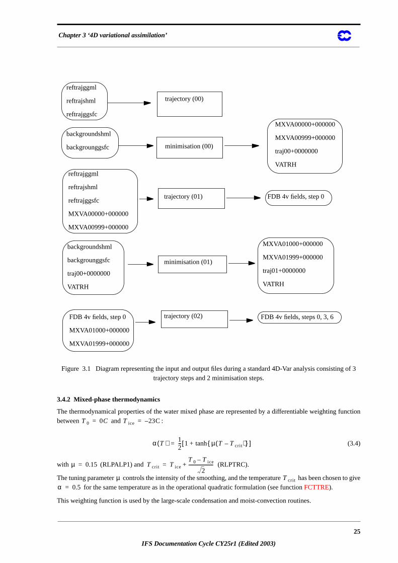
The ouput of the minimization steps are the filesMXVAxx000+000000, MXVAxx999+000000(as in 3D-Var),
trajxx+0000000andVATRH . xx is an integer varying from 0 for the first minimization to (n-1) for the last min
imization, where n is the number of updates of the trajectory.VATRH contains useful information for a warm re-
start of m1qn3 (including the diagonal of the Hessian).trajxx+0000000contains the control variable at the end o
the minimization. The filetrajxx+0000000is written out inSAVMINI called at the end ofCVA1. This file will be
n n
23
IFS Documentation Cycle CY25r1 (Edited 2003)
Part II: ‘Data assimilation’
ad in
he tra-
. An-
ctory,
he di-
lds cre-
ements
. The
nd of
files.
itches
IF2,
is
non-
set of
scale
F2).
pack-
g the
y steps
an input to the next minimization in addition to the background file used as in the first minimization. It is re
in GETMINI called fromCVA1. The fileVATRH is written out inSAVMIN , and read inSUHESS, both called
by CVA1.
The input of the second trajectory is the same as in 3D-Var. The output is an analysis at the initial time of t
jectory (type = 4v, step = 0) written out on the FDB. It contains the current estimate of the flow at initial time
other output are the updated observation files, as in 3D-Var. The 4v fields are used in the following traje
replacing the background in the input filesICMSHxxxxINIT , ICMGGxxxxINIT and ICMGGxxxxINIUA(wherexxxx is the ‘expver’ identifier of MARS). Additional inputs are low resolution files (MXVA ...) created dur-
ing the previous minimization interpolated to high resolution as in 3D-Var. This data flow is represented in t
agram below.
In summary, the first two trajectories use the background as an input, and the following ones use the 4v fie
ated during the previous trajectory as reference files. All the trajectories except for the very first one add incr
computed from the low-resolution files produced by the previous minimization, interpolated to high resolution
first minimization uses only the background field, the following ones also use the control variable from the e
the previous minimization and some information for a warm restart of the minimization package.
The number of updates of the trajectory starting from 0 at the first minimization is carried inside the ODB
3.4 TANGENT LINEAR PHYSICS
The first minimization uses the simplified physics (vertical diffusion and surface drag) activated by the sw
LSPHLC, LVDFDS, LSDRDS, LVDFLC, LSDRLC, LKEXP in namelistNAPHLC which is also activated for sin-
gular vector computations. A scientific description of the simplified physics is given inBuizza1994) .
The following minimizations use a more complete linear physics activated by the switches LETRAJP, LEVD
LEGWDG2, LECOND2, LERADI2, LERADS2, LECUMF2 in namelistNAMTRAJP, and described in this sec-
tion. The description is focused on technical aspects, since scientific issues can be found elsewhere (Mahfoufet al.,
1997;Rabier et al.1997;Mahfouf 1998).
3.4.1 Set-up
In order to activate the improved linear physics, the switch LSPHLC of the simplified linear physics inNAPHLC
should be set to FALSE. InCVA1 when both logicals LSPHLC and LETRAJP are equal to TRUE, LSPHLC
reset to FALSE and a warning is written in the standard ouput (logical unit NULOUT).
The following switches must be set to TRUE : LEPHYS, LAGPHY (also necessary to activate the ECMWF
linear physics) and LETRAJP (to activate storage of the trajectory at ). The linear physics contains a
five physical processes : vertical diffusion (LEVDIF2), sub-grid scale orographic effects (LEGWD2), large
condensation (LECOND2), longwave radiation (LERADI2, LERADS2), and deep moist convection (LECUM
Tunable parameters of the improved physics (which should not in principle be modified) are defined inSUPHLI.
The logical LPHYLIN is used to activate the simplifications and/or modifications associated with the linear
age in the non-linear physics. This variable is set to FALSE by default , but is forced to TRUE before callin
linear physics (CALLPARTL and CALLPARAD) in CPGLAGTL and CPGLAGAD whenever the logical
LETRAJP is TRUE.
Diagram representing the input and output files during a standard 4D-Var analysis consisting of 3 trajector
and 2 minimisation steps.
t ∆t–
24
IFS Documentation Cycle CY25r1 (Edited 2003)
Chapter 3 ‘4D variational assimilation’
g of 3
nction
to give
Figure 3.1 Diagram representing the input and output files during a standard 4D-Var analysis consistin
trajectory steps and 2 minimisation steps.
3.4.2 Mixed-phase thermodynamics
The thermodynamical properties of the water mixed phase are represented by a differentiable weighting fu
between and :
(3.4)
with (RLPALP1) and (RLPTRC).
The tuning parameter controls the intensity of the smoothing, and the temperature has been chosen
for the same temperature as in the operational quadratic formulation (see functionFCTTRE).
This weighting function is used by the large-scale condensation and moist-convection routines.
trajectory (00)
minimisation (00)
trajectory (01)
minimisation (01)
trajectory (02)
reftrajggml
reftrajshml
reftrajggsfc
backgroundshml
backgrounggsfc
MXVA00000+000000
MXVA00999+000000
traj00+0000000
VATRHreftrajggml
reftrajshml
reftrajggsfc
MXVA00000+000000
MXVA00999+000000
FDB 4v fields, step 0
backgroundshml
backgrounggsfc
traj00+0000000
VATRH
MXVA01000+000000
MXVA01999+000000
traj01+0000000
VATRH
FDB 4v fields, step 0
MXVA01000+000000
MXVA01999+000000
FDB 4v fields, steps 0, 3, 6
T0 0C= T ice 23C–=
α T( ) 12--- 1 µ T Tcrit–( ){ }tanh+[ ]=
µ 0.15= Tcrit T ice
T0 T ice–
2----------------------+=
µ Tcrit
α 0.5=
25
IFS Documentation Cycle CY25r1 (Edited 2003)

Part II: ‘Data assimilation’
cients
he local
n–
ndary
3.4.3 Vertical diffusion
The linear versions of the vertical diffusion scheme are called from the driversVDFMAINTL andVDFMAINAD .
Vertical diffusion applies on wind components, dry static energy and specific humidity. The exchange coeffi
in the planetary boundary layer and the drag coefficients in the surface layer are expressed as functions of t
Richardson number (Louis et al., 1982). They differ from the operational formulation which uses the Moni
Obukhov length as a stability parameter in stable conditions and a -profile approach for convective bou
layers (see the documentation of the ECMWF physics).
In stable conditions ( ), the drag coefficients are defined as :
(3.5)
and
(3.6)
with the following expressions for the neutral coefficients :
(3.7)
(3.8)
In unstable conditions ( ), the drag coefficients are defined as:
(3.9)
(3.10)
The empirical coefficients (RLPBB), (RLPCC) and (RLPDD) are set to 5 inSUPHLI.
In the planetary boundary layer, the exchange coefficients can formally be writen :
K
Ri 0>
CM CMN1
1 2bRi1 dRi+
------------------------+----------------------------------=
CH CHN1
1 3bRi 1 dRi++------------------------------------------------=
CMNk2
z z0M+
z0M------------------
log2
----------------------------------------=
CHNk2
z z0M+
z0M------------------
z z0M+
z0H------------------
loglog
-----------------------------------------------------------------------=
Ri 0<
CM CMN 1 2bRi
1 3bcCMN
z z0M+
z0M------------------ Ri+
-----------------------------------------------------------------–
=
CH CHN 1 3bRi
1 3bcCHN
z z0M+
z0H------------------ Ri+
----------------------------------------------------------------–
=
b c d
26
IFS Documentation Cycle CY25r1 (Edited 2003)
Chapter 3 ‘4D variational assimilation’
epth
gth
g of
e-
et to
ribed in
DRAG
-
ers is
0.95 in
given
mpera-
(3.11)
with the following mixing length vertical profile :
(3.12)
The asymptotic mixing lengh for momemtum is set to 150 m, whereas . The pseudo-d
of the boundary layer is defined by km(RLPMIXL), and the reduction factor applied to the mixing len
in the free atmosphere is ( RLPBETA) [ when ].
If this vertical-diffusion scheme is activated in the nonlinear model (LPHYLIN = .TRUE.), the post-processin
atmospheric parameters at observation level can be performed using the formulation ofGeleyn(1988) inVDFP-
PCFLS(the tangent-linear and adjoint versions ofVDFPPCFLSare not yet coded, but are already available els
where in the IFS for the observation operators).
This modified scheme make use of all the routines from the operational vertical diffusion, exceptVDFSFLX and
VDFHGHT, however the exchange coefficients are computed in a different way inVDFEXCSandVDFEXCU.
The linearization of the surface energy balance is also performed (VDFTSKTL, VDFTSKAD), but perturbations
of the skin temperature are not evolved in time (section 4.4 inCPGLAGTL). This simplification should be relaxed
when the skin temperature becomes part of the control variable.
The logical LEKPERT inNAMTRAJPcontrols the perturbations of the exchange and drag coefficients. It is s
FALSE by default, to prevent the growth of spurious instabilities in the tangent-linear model..
3.4.4 Sub-grid scale orographic effects
The subgrid-scale orographic scheme is a complete linearization of the operational ECMWF scheme desc
Lott and Miller (1997). The linearized schemes are called fromGWDRAGTL andGWDRAGAD. By setting the
constant RLPDRAG to zero, the representation of wave breaking is not activated (The operational value GK
is set to 0.3 inSUGWDand is used to compute the surface stress in the gravity-wave part of the scheme).
3.4.5 Large-scale precipitation
Linearized versions of large-scale condensation scheme areCONDTL andCONDAD. Local supersaturation is re-
moved through a local moist-adjustment scheme (CUADJTQTL , CUADJTQAD). Supersaturation produces pre
cipitation instantaneously (without a cloud stage). The effect of rainfall evaporation in sub-saturated lay
strongly reduced in the linearized versions of the scheme. The constant RLPEVAP is set to 0.05, instead of
the nonlinear parametrization (it indicates that evaporation will take place as long as specific humidity in a
layer is below RLPEVAP times its saturation value).
3.4.6 Long-wave radiation
The linear long-wave radiation is based on a constant emissivity approach, where only perturbations on te
ture are accounted for. Tendencies produced by the linearized long-wave radiation inRADHEATTL andRAD-
HEATAD are damped above a pressure level (RLPP00) set to 300 hPa inSUPHLI:
K l2 ∂V∂z------- f Ri( )=
lk z z0+( )
1 kz z0+( )
λ-------------------+
-------------------------------- γ 1 γ–
1z z0+( )2
L2---------------------+
-------------------------------+=
λM λH λM 1.5d=
L 4=
γ 0.2= l γλ→ z L»
pc
27
IFS Documentation Cycle CY25r1 (Edited 2003)
Part II: ‘Data assimilation’
part of
es for
d in the
e non-
e driv-
ry.
el
uted in
-
the ten-
s (which
tion;
(3.13)
where the net flux arrays (PEMTED5) computed from the full non-linear radiation scheme are stored as
the trajectory during the non-linear integration (see description of the trajectory management).
3.4.7 Deep moist convection
The partial linearization of the ECMWF mass-flux scheme is performed, leading to the following tendenci
the perturbations of the prognostic variables (wind components, specific humidity, dry static energy):
(3.14)
The mass-fluxes profiles associated with the updrafts and the downdrafts and are recompute
tangent-linear and adjoint integrations from the stored basic state. This partial linearization implies that all th
linear routines for the convection scheme have their tangent-linear and adjoint counterparts (starting form th
ing routinesCUCALLNTL andCUCALLNAD). However, most of them are only used to recompute the trajecto
The only routines which contain linear statements areCUININTL (mean thermodynamical properties at half mod
levels),CUDUDVTL (tendencies for the wind components) andCUDTDQNTL (tendencies for dry static energy
and specific humidity).Eq. (3.14) is solved numerically in the following form (seeTiedtke, 1989) :
(3.15)
which requires extra local storage of the profiles of entrainment and detrainement rates and comp
CUASCN and
in CUDDRAFN (variables PDMFEN and PDMFDE).Eq. (3.15)is only applied when deep convection is diag
nosed from the basic state.
3.4.8 Trajectory management
The ECMWF physics uses the tendencies from the dynamics, and variables at as input to compute
dencies of a given process (represented by the operator ) for a prognostic variable :
(3.16)
where the variable has already been updated by the dynamics and by the previous physical processe
are called in the following order: radiation; vertical diffusion; subgrid-scale orographic effects; moist convec
large-scale condensation).
Thus :
(3.17)
∂T′∂t
---------1
1ppc------
10+
------------------------- gcp-----
p∂∂ 4F
T-------T′
=
F
∂ψ′∂t
---------1ρ--- Mup Mdown+( ) ψ′∂
∂z--------=
Mup Mdown
∂ψ′∂t
---------1ρ---
∂ Mupψ′( )∂z
------------------------∂ Mdownψ′( )
∂z------------------------------ Dup Eup– Ddown Edown–+( )ψ′+ +=
E D
t ∆t–
P ψ
ψn 1+ ψun 1––
2∆t----------------------------------- P ψu
n 1–( )=
ψu
ψun 1– ψn 1– ∂ψ
∂t-------
dyn
∂ψ∂t-------
phys
+ +=
28
IFS Documentation Cycle CY25r1 (Edited 2003)
Chapter 3 ‘4D variational assimilation’
the
amics
to the
in
idity)
es and
from
te the
fluxes,
rs) are
fields
fined
with
BT95,
In Eq. (3.16), if the operator is nonlinear, its linearization around the basic state , will require to store
model state at time step (trajectory at ) as well as the tendencies produced by the dyn
. The physical tendencies from the previous processes , require an additional call
nonlinear routines in the adjoint computations (CALLPARAD) and a local storage of the partial tendencies.
The storage of the trajectory at is performed inCPGLAGby the routineWRPHTRAJcalled before the driv-
er of the ECMWF physicsCALLPAR. Fields are stored in grid-point space in an array TRAJPHYS allocated
SUSC2.
The following three-dimensional fields are stored :
• For the atmosphere: the prognostic variables (wind components, temperature, specific hum
and their tendencies produced by adiabatic processes, the vertical velocity, the long-wave flux
the solar transmissivity (these two last fields allow the computation of the radiation tendencies
the trajectory inCALLPARTL andCALLPARAD)
• For the soil: the prognostic variables for temperature and moisture content (used to compu
surface fluxes from the trajectory in the linear vertical-diffusion scheme)
A number of two-dimensional fields used at time step need to be stored: surface pressure, surface
skin temperature, skin reservoir, snow reservoir, roughness lengths (mainly for the vertical diffusion).
The preliminary computations (pressure and geopotential at full and half model levels, astronomy paramete
perfomed inCPGLAGTL andCPGLAGAD before calling the driver of the tangent-linear physicsCALLPARTL
or the driver of the adjoint physicsCALLPARAD, and after reading the trajectory fields fromRDPHTRAJ.
The number of fields to be stored is defined inSUTRAJPfor 3-D atmospheric fields on full model levels
(NG3D95), 3-D atmospheric fields on half model levels (NG3P95), 3-D soil fields (NG3S95), and surface
(NG2D95).
The option to store the trajectory on disk (instead of in memory) also exists through the logical LIOTRPH de
in SUTRAJPbut is not used anymore on FUJITSU VPP computers. Packing of the trajectory is also possible
the variable NPCKFT95 (set to 1 by default, which means no packing) and the packing parameter NEXP
provided packing libraries are compiled with the IFS (routinesEXPANDX1).
P ψun 1–
n 1– t ∆t–
∂ψ ∂t⁄( )dyn ∂ψ ∂t⁄( )phys
t ∆t–
t ∆t–
29
IFS Documentation Cycle CY25r1 (Edited 2003)

Part II: ‘Data assimilation’
30
IFS Documentation Cycle CY25r1 (Edited 2003)

IFS Documentation Cycle CY25r1
this
,
sure,
f
-
the
-
tructed
riable
Part II: D ATA ASSIMILATION
CHAPTER 4 Background term
Table of contents
4.1 Introduction
4.2 Description of the algorithm
4.3 Technical implementation
4.3.1 Input files
4.3.2 Namelist parameters of
4.3.3 IFS routines
4.3.4 Background error
4.1 INTRODUCTION
The background term described inCourtieret al.(1998) was in May 1997 replaced by a new formulation byBout-
tier et al. (1997), available online as newjb.ps. The old code is still part of the IFS but will not be described in
documentation.
4.2 DESCRIPTION OF THE ALGORITHM
We use the following notation:
• is the low–resolution analysis increment, i.e. model field departures from the background
• is the assumed background error covariance matrix,
• , , and are increments of vorticity, divergence, temperature and surface pres
and specific humidity, respectively, on model levels.
• and are thebalancedparts of the and increments. The concept o
balance will be defined below, and
• and are theunbalancedparts of and , i.e. and
, respectively.
The incremental variational analysis problem,Eq. (1.2)of Chapter 1 ‘Incremental formulation of 3D/4D variation
al assimilation—an overview’, is rewritten in the space defined by the change of variable (Section 1.4)
where satisfies so that takes the simple form ofEq. (1.8). In operational practice, the initial point
of the minimization is the background, so that initially . The minimization can be carried out in
space of , where is the euclidean inner product,Eq. (1.8). At the end of the minimization, the analysis incre
ments are reconstructed in model space by . In order to compare with observations is recons
usingEq. (2.4), in each simulation. Thus the variational analysis can be done with , the inverse change of va
from minimization space to model space (chavarin}, without ever usingCHAVAR.
The background-error covariance matrix is implied by the design of , which currently has the form
δxBζ η T psurf,( ) q
ηb T psurf,( )bal η T psurf,( )
ηu T psurf,( )unbal η T psurf,( ) η ηbal–
T psurf,( ) T psurf,( )bal–[ ]
δx L χ=
L LL T B= Jb
δx χ 0= =
χ Jb
δx L χ= xL
B L
31
IFS Documentationn Cycle CY25r1 (Edited 2003)
Part II: ‘Data assimilation’
ables
r co-
lance
ed var-
lies sig-
with no
l coef-
sulting
ructures
elations
(
MC
co-
ociated
(4.1)
where is a balance operator going from the set of variables , , and , to the model vari
, , and . The operator is the right–hand symmetric square root of the background-erro
variances of , , and , so that
(4.2)
So far, the formulation is perfectly general. Now, we restrict to a simple form and choose a particular ba
operator .
The covariance matrix is assumed to be block-diagonal, with no correlation between the parameters:
(4.3)
It implies that the analysis is independent from the other variables. However, assuming that the unbalanc
iables are uncorrelated is not too restrictive because, as we shall see below, the design of the balance imp
nificant multivariate correlations between the meteorological variables.
Each autocovariance block in the above matrix is itself assumed to be block-diagonal in spectral space,
correlation between different spectral coefficients, but a full vertical autocovariance matrix for each spectra
ficient. The vertical covariance matrices are assumed to depend only on the total wavenumber . The re
autocovariance model is homogeneous, isotropic and non-separable in grid-point space: the correlation st
do not depend on the geographical location, but they depend on the scale. The shape of the horizontal corr
is determined by the covariance spectra. The same representation was used in the previous formulationRabier
and McNally1993,Courtier et al. 1998). The covariance coefficients are computed statistically using the N
method (Parrishand Derber1992,Rabieret al.1998) on 24/48-hour forecast differences to estimate the total
variances for each total wavenumber , and assuming an equipartition of errors between the ass
spectral coefficients.
The balance relationship is arbitrarily restricted to the following form:
(4.4)
So that the complete balance operator is defined by:
(4.5)
or equivalently, in matrix form:
L KB u1 2/=
K ζ ηu T psurf,( )u qζ η T psurf,( ) q Bu
1 2/
Bu ζ ηu T psurf,( )u q
Bu Bu1 2⁄( )TBu
1 2/=
Bu
K
Bu
Bu
Cζ 0 0 0
0 Cηu0 0
0 0 C T psurf,( )u0
0 0 0 Cq
=
q
n
Jb
n 2n 1+
ηb M ζ=
T psurf,( )b Nζ Pηu+=
K
ζ ζ=
η M ζ ηu+=
T psurf,( ) Nζ Pηu T psurf,( )u+ +=
q q=
32
IFS Documentation Cycle CY25r1 (Edited 2003)

Chapter 4 ‘Background term’
is
.
a-
riances
erm
ponsi-
re both
cients
vari-
ard ana-
om: in
ectral
r-range
sion
onal
ized
(4.6)
The matrix blocks , and are, in general, not invertible, but is. As explained above, the inverse of
not actually used in the variational analysis, because the initial point of the minimization is the background
The matrix multiplication of by allows one to write explicitly the implied background error covariance m
trix in terms of the meteorological variables , , and :
(4.7)
The blocks implied by and its transforms by the balance operator blocks , and are thebalancedparts
of the covariances. For instance, the vorticity covariances and the unbalanced temperature cova
are both homogeneous and isotropic, whereas the ‘vorticity-balanced’ matrix t
depends on latitude—it is predominant in the extratropics, negligible near the equator. The term is res
ble for the geostrophic mass/wind coupling.
The , and operators used to define the balance have a restricted algebraic structure. and a
the product of a so-called horizontal balance operator by vertical balance operators , :
(4.8)
The operator is a block–diagonal matrix of identical horizontal operators transforming the spectral coeffi
of vorticity, independently at each level, into an intermediate variable which is a kind of linearized mass
able defined below. The horizontal operators in have exactly the same algebraic structure as the stand
lytical linear balance on the sphere, and this is where the latitudinal variations of the structures come fr
spectral space,
(4.9)
The , and operators all have the same structure: block-diagonal, with one full vertical matrix per sp
component. The vertical matrices depend only on the total wavenumber .
The actual calibration of the operator requires the following 4 steps; each one uses a set of 24/48-hou
forecast differences as surrogates to background error patterns in order to calculate the statistics:
1) operator. The horizontal balance coefficients of are computed by a linear regres
between the errors in vorticity and in linearized total mass , assuming the functi
relationship defined by the above equation, and building from using the linear
hydrostatic relationship at level ,
K
I 0 0 0
M I 0 0
N P I 0
0 0 0 I
=
M N P K K
Bu KB ζ η T psurf,( ) q
B KB uK T
Cζ CζM T CζNT 0
MC ζ MC ζM T Cηu+ MC ζNT Cηu
PT+ 0
NCζ NCζM T PCηu+ NCζNT PCηu
PT C T psurf,( )u+ + 0
0 0 0 Cq
= =
Cζ M N PCζ
C T psurf,( )uNCζNT T psurf,( )
NCζ
M N P M NH M N
M MH=
N NH=
HPb
HJb
Pb n m,( ) β1 n m,( )ς n m 1+,( ) β2 n m,( )ς n m 1–,( )+=
M N Pn
Jb
H β1 β2,( ) HPtot
Ptot T psurf,( )l
33
IFS Documentation Cycle CY25r1 (Edited 2003)
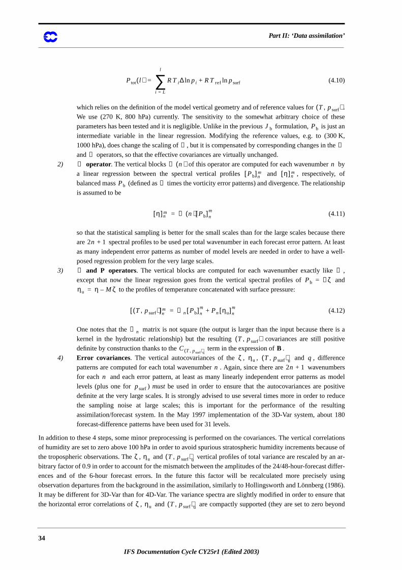
Part II: ‘Data assimilation’
.
hese
st an
0 K,
the
by
y, of
nship
e there
t least
a well-
,
and
re is a
itive
ce
mbers
model
itive
educe
lting
t 180
elations
ause of
an ar-
differ-
using
986).
that
eyond
(4.10)
which relies on the definition of the model vertical geometry and of reference values for
We use (270 K, 800 hPa) currently. The sensitivity to the somewhat arbitrary choice of t
parameters has been tested and it is negligible. Unlike in the previous formulation, is ju
intermediate variable in the linear regression. Modifying the reference values, e.g. to (30
1000 hPa), does change the scaling of , but it is compensated by corresponding changes in
and operators, so that the effective covariances are virtually unchanged.
2) operator. The vertical blocks of this operator are computed for each wavenumber
a linear regression between the spectral vertical profiles and , respectivel
balanced mass (defined as times the vorticity error patterns) and divergence. The relatio
is assumed to be
(4.11)
so that the statistical sampling is better for the small scales than for the large scales becaus
are spectral profiles to be used per total wavenumber in each forecast error pattern. A
as many independent error patterns as number of model levels are needed in order to have
posed regression problem for the very large scales.
3) and operators. The vertical blocks are computed for each wavenumber exactly like
except that now the linear regression goes from the vertical spectral profiles of
to the profiles of temperature concatenated with surface pressure:
(4.12)
One notes that the matrix is not square (the output is larger than the input because the
kernel in the hydrostatic relationship) but the resulting covariances are still pos
definite by construction thanks to the term in the expression of .
4) Error covariances. The vertical autocovariances of the , , and , differen
patterns are computed for each total wavenumber . Again, since there are wavenu
for each and each error pattern, at least as many linearly independent error patterns as
levels (plus one for )mustbe used in order to ensure that the autocovariances are pos
definite at the very large scales. It is strongly advised to use several times more in order to r
the sampling noise at large scales; this is important for the performance of the resu
assimilation/forecast system. In the May 1997 implementation of the 3D-Var system, abou
forecast-difference patterns have been used for 31 levels.
In addition to these 4 steps, some minor preprocessing is performed on the covariances. The vertical corr
of humidity are set to zero above 100 hPa in order to avoid spurious stratospheric humidity increments bec
the tropospheric observations. The , and vertical profiles of total variance are rescaled by
bitrary factor of 0.9 in order to account for the mismatch between the amplitudes of the 24/48-hour-forecast
ences and of the 6-hour forecast errors. In the future this factor will be recalculated more precisely
observation departures from the background in the assimilation, similarly to Hollingsworth and Lönnberg (1
It may be different for 3D-Var than for 4D-Var. The variance spectra are slightly modified in order to ensure
the horizontal error correlations of , and are compactly supported (they are set to zero b
Ptot l( ) RTi∆ pi RT ref psurfln+ln
i L=
l
∑=
T psurf,( )
Jb Pb
H MN
M M n( ) nPb[ ]n
m η[ ]nm
Pb H
η[ ]nm M n( ) Pb[ ]n
m=
2n 1+
N P MPb Hζ=
ηu η Mζ–=
T psurf,( )[ ]nm N n Pb[ ]n
m Pn ηu[ ]nm+=
N n
T psurf,( )C T psurf,( )u
Bζ ηu T psurf,( )u q
n 2n 1+
npsurf
ζ ηu T psurf,( )u
ζ ηu T psurf,( )u
34
IFS Documentation Cycle CY25r1 (Edited 2003)

Chapter 4 ‘Background term’
is per-
rently
o alter
orecasts
st error
nning
ad and
nts of
ple of
In the
ents for
scribed
tring
ed
ors),
sup-
The
6000 km). This operation removes the residual sampling noise in the error covariances. No other processing
formed except for a spectral truncation if the analysis resolution is lower than the statistics resolution (cur
T106). It would be easy to extrapolate the statistics to higher resolutions, but it would be very hazardous t
the vertical geometry of the covariances and balance operators. Instead, it is recommended to run a set of f
using a model with the right vertical resolution, and recompute all the statistics from scratch.
4.3 TECHNICAL IMPLEMENTATION
The statistical calibration is done using dedicated scripts outside the IFS code. First, the 24/48-hour foreca
differences for a set of dates are constructed in terms of spectral , , and . This involves ru
a set of MARS requests and building the required GRIB files. Then, the forecast-error differences are re
processed by a Fortran statistics program that finally writes two files in GSA format: one with the coefficie
the balance operator, one with the error covariances of , , and . These files take up a cou
megabytes. They are computed for a given triangular truncation and number of levels (currently T106L31).
covariance file there are 4 sets of vertical covariance matrices. The balance files contain one set of coeffici
the operator, and three sets of vertical balance matrices for , and .
4.3.1 Input files
The IFS needs these two GSA files to use in e.g. the incremental analysis jobs. The configuration de
here corresponds to namelist switch LSTABAL=.true. (NAMJG), and it is identified in the code by the s
CDJBTYPE=‘STABAL96’. LSTABAL=.false. would give the old formulation. The input files must be nam
stabal96.cv andstabal96.bal. They are read in bysujbdat andsujbbal, respectively.
4.3.2 Namelist parameters of
Some other important namelist options in NAMJG are LCFCE (to enforce uniform background err
L3DBGERR (to have a 3D distribution vorticity background errors), and LCORCOSU (to enforce compactly
ported horizontal correlations). The switch LGUESS in NAMCT0 can be used to switch off altogether.
default is LGUESS=.true., i.e. switched on.
ζ η T psurf,( )u q
ζ ηu T psurf,( )u q
H M N P
Jb Jb
Jb
Jb
Jb
Jb
Jb
35
IFS Documentation Cycle CY25r1 (Edited 2003)
Part II: ‘Data assimilation’
Figure 4.1 Calling tree for subroutinesujbcov.
(This is the setup code tree in IFS cy16r3, option stabal96)
(namelist namjg has already been read into yomjg in routine sujb below su0yoma)
sujbcov determine configuration (nonsep93, stabal96 or totenrgy)
allocate work arrays
sujbdat read covariance file ‘stabal96.cv’
commjbdat distribute covariances to all processors
suprecov prepare vertical interpolation
truncate / extrapolate spectrally to IFS resolution
reset q stratospheric correlations
sujbcor < lcorcosu > prepare Legendre polynomials
normalize covariance matrices into correlations
eigenmd factorize inverse vertical correlation matrices—> arrays FGEDVNx, FGEGVM
generate horizontal correlation spectra
< lcorcosu > sujbcosu generate compactly supportedhorizontal correlation spectra
inverse square root of horiz correl spectra —> array FGSCNM
print average vertical correlation matrices
< kprt>1 > print spectra and gridpoint structures ofhorizontal correlations
sujbstd calculate total variances at each level
standard deviation vertical profiles times REDNMC—> arrray FCMN / FCEMNP
suecges horizontal stdev structures (see cycling doc)
sujbbal read balance file ‘stabal96.bal’
commjbbal distribute balance to all processors
convert to IFS truncation —> arrays SDIV, STPS, BFACT/2
sujbmod (modification of vertical correlations, not supported)
sujbmap (modification of geometry, not yet implemented)
sujbdiag (diagnostic of structure functions, not supported)
sujbstat (online update of statistics, not yet implemented)
sujbwrit (rewrite of operators, not yet implemented)
< ljbtest > sujbtest (Technical test of code)
setup random vector
cvar2in / cvar2inad adjoint test on them
cvar2 / cvar2in inverse tests on them
cvar2ad / cvar2inad inverse tests on them
Jb
Jb
Jb
Jb
Jb
Jb
Jb
36
IFS Documentation Cycle CY25r1 (Edited 2003)
Chapter 4 ‘Background term’
t-up
ontal
es are
er
l data is
erators,
4.3.3 IFS routines
Inside the IFS code, is localized in the setups below subroutinesujbcovand in the inverse change of variable
cvar2in(and its adjoint and their inverses,CVAR2INAD, CVAR2 andCVAR2AD). Calling trees are shown inFig.
4.1 andFig. 4.2. The computation of the cost function and its adjoint is done insim4d(Section 2.3in Chapter 2
‘3D variational assimilation’)---it is planned to move it to a dedicated subroutine. The sequence within the se
routine is the following:
(i) SUJBDAT: Reads covariances from filestabal96.cv,Interpolates in the vertical to the model’s vertical levels (if necessary)
Sets humidity correlations to 0, for pressures less than 100 hPa.
(ii) SUJBCOR: Sets up spectral correlation operator
Covariance matrices (one per ) are converted to vertical correlation matrices and horiz
autocorrelation spectra. The eigenvectors and the eigenvalues of vertical correlations matric
computed usingEIGENMD and stored in FGEDVNS and FGEGVNS-arrays (yomjg), respectively,
for later use in JGVCOR, JGVCORI, JGVCORAD and JGVCORIAD. The horizontal
autocorrelation spectra are stored in the FGSCNM–array (yomjg), for later use inJGHCORand
JGHCORI.
(iii) SUJBSTD: Set up background error standard deviations, seeSubsection 4.3.4.
(iv) SUJBBAL: Set up balance constraint. Read the filestabal96.baland store inyomjg, for later use in
balstat, balstatad, balvert, balvertad, balverti and balvertiad as part of the change of variable
operator.
(v) SUJBTEST: Test of the adjoint of the change of variable, if LJBTEST=.true.
The distributed memory affects the setups belowsujbdatandsujbbalwhen the data files are read in (by the mast
processor only). First, the resolution of the files is read, then the relevant arrays are allocated and the actua
read, truncated if necessary, and broadcast. The code is designed to work at any resolution.
In the change of variable, there is a transposition of the fields between the horizontal and vertical balance op
balstatandbalvert, repsectively. Note that the operator is performed by callingcvar2in, so in IFS parlance
corresponds to theinverse change of variable.
Jb
Jb
n
L L
37
IFS Documentation Cycle CY25r1 (Edited 2003)
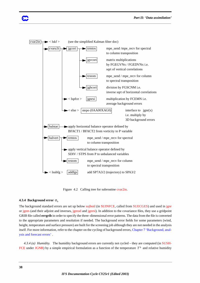
Part II: ‘Data assimilation’
nt
erted
s (wind,
analysis
idity
Figure 4.2 Calling tree for subroutinecvar2in.
4.3.4 Background error
The background standard errors are set up belowsujbstd(in SUINFCE, called fromSUECGES) and used injgnr
or jgnrs(and their adjoint and inverses,jgnradandjgnrsi). In addition to the covariance files, they use a gridpoi
GRIB file callederrgrib in order to specify the three–dimensional error patterns. The data from the file is conv
to the appropriate parameters and resolution if needed. The background error fields for some parameter
height, temperature and surface pressure) are built for the screening job although they are not needed in the
itself. For more information, refer to the chapter on the cycling of background errors,Chapter 7 ‘Background, anal-
ysis and forecast errors’ .
4.3.4 (a) Humidity. The humidity background errors are currently not cycled – they are computed (inSUSH-
FCEunderJGNR) by a simple empirical formulation as a function of the temperature and relative hum
cvar2in < lskf > (see the simplified Kalman filter doc)
cvaru3i jgcori trmtos mpe_send /mpe_recv for spectral
to column transposition
jgvcori matrix multiplications
by FGEGVNx / FGEDVNx i.e.
sqrt of vertical correlations
trstom mpe_send / mpe_recv for column
to spectral transposition
jghcori division by FGSCNM i.e.
inverse sqrt of horizontal correlations
< lspfce > jgnrsi multiplication by FCEMN i.e.
average background errors
< else > stepo (0AA00XAG0) interface to jgnr(x)
i.e. multiply by
3D background errors
balstat apply horizontal balance operator defined by
BFACT1 / BFACT2 from vorticity to P variable
balvert trmtos mpe_send / mpe_recv for spectral
to column transposition
apply vertical balance operator defined by
SDIV / STPS from P to unbalanced variables
trstom mpe_send / mpe_recv for column
to spectral transposition
< lsubfg > addfgs add SP7A3/2 (trajectory) to SPA3/2
σb
Tb
38
IFS Documentation Cycle CY25r1 (Edited 2003)
Chapter 4 ‘Background term’
on of
ature
strat-
f
500hPa
exceeds
l
d by
of the background:
(4.13)
(4.14)
The standard deviation in terms of relative humidity is then converted to specific humidity, taking the variati
of the equation
(4.15)
where is the relative humidity, , is the saturation water-vapour pressure at the temper
in question (Tetens’ formula,Eq. (5.11)in Chapter 5 ‘Conventional observational constraints’) and is pressure.
Humidity increments are forced to be negligibly small above the tropopause to avoid a systematic drift of
ospheric humidity over extended periods of data assimilation. This is achieved by setting a very low value o
for everywhere the pressure is lower than 70hPa, and at anyother point where the pressure is lower than
and the background temperature and pressure fields are such that the square of the buoyancy frequency
everywhere between that level and the 70hPa level.
More specifically, for each grid column is set to for model levels such that , where the leve
is determined by requiring either that it is the highest level with hPa for which
(4.16)
or, if no such level can be found for in the range from 500 to 70hPa, that it is the lowest level for which
.
Here and are the background temperature and pressure at level of the grid-column.
In addition, any values of lower than are reset to .
For pressures less than = 800 hPa, and over the sea, the model of background errors above is modifie
(4.17)
where (where LSM = land–sea mask) and =12500.
Ub
σb 0.002Tb– 0.0033Tb 273–– 0.25Ub 0.35Ub 0.4–– 0.70+ +=
σb min 0.18 max 0.06σb,( ),[ ]=
q
qUesat
1ε--- p U 1
ε--- 1–
esat–
--------------------------------------------=
U ε Rdry Rvap⁄= esat
p
10 8–
σb
2 10 4–× s 2–
σb 10 8– k k K≤ KpK
b 70≥
pK 1+b TK 2+
b TKb–( )
TK 1+b pK 2+
b pKb–( )
------------------------------------------------RdryTK 1+
b
g2-------------------------- 2.5 10 4–×( ) κ>+
pKb
pKb 500 hPa≤
TKb pK
b K
σb 10 8– 10 8–
p0
σmod σb 1 a– apb p0–
b------------------
2
–exp+
=
α 0.5 1 LSM–( )= b
39
IFS Documentation Cycle CY25r1 (Edited 2003)

Part II: ‘Data assimilation’
40
IFS Documentation Cycle CY25r1 (Edited 2003)
IFS Documentation Cycle CY25r1
allows
ple. In
used in
Part II: D ATA ASSIMILATION
CHAPTER 5 Conventional observational constraints
Table of contents
5.1 Introduction
5.2 Data usage
5.2.1 Controls
5.2.2 Overview of observation operators
5.3 The observation operator for geopotential height
5.3.1 Quadratic vertical interpolation near the top of the model
5.3.2 Below the model’s orography
5.4 The observation operator for wind
5.5 The observation operators for humidity
5.5.1 Saturation vapour pressure
5.5.2 Relative humidity
5.5.3 Precipitable water
5.5.4 Specific humidity
5.6 The observation operator for temperature
5.7 Surface observation operators
5.7.1 Mathematical formulation
5.7.2 Surface values of dry static energy
5.7.3 Transfer coefficients
5.7.4 Two-metre relative humidity
5.1 INTRODUCTION
The observation operators provide the link between the analysis variables and the observations (Lorenc, 1986,Pail-
leux, 1990). The operator inEq. (1.4)signifies the ensemble of operators transforming the control variable
into the equivalent of each observed quantity, , at observation locations. The 3D/4D–Var implementation
to be (weakly) non-linear, which is seen to be an advantage for the use of TOVS radiance data, for exam
this chapter we define the content of each of the observation operators and describe the observational data
3D/4D–Var. The use of satellite data is described inChapter 6 ‘Satellite observational constraints’ .
H xyo
H
41
IFS Documentationn Cycle CY25r1 (Edited 2003)

Part II: ‘Data assimilation’
D–Var.
tal col-
ata
AT and
sage is
sis time.
were
hourly
ta-
lected
re per-
vari-
com-
S code
he first
r defini-
o
rmation
s
n grid
el
(
5.2 DATA USAGE
Observation operators for all observation types that were used by OI have also been implemented in 3D/4
In addition 3D/4D–Var uses TOVS cloud-cleared radiances, scatterometer ambiguous winds and SSMI to
umn water vapour.Table 10.6lists the observing systems currently used by 4D–Var in ECMWF’s operational d
assimilation. The table also indicates important restrictions on data usage and thinning of data. TOVS, SC
SSMI data are further discussed inChapter 6 ‘Satellite observational constraints’. Additional data types such as
meteosat radiances and TOVS and ATOVS 1C-radiances are used experimentally. ATOVS 1C radiance u
described in a separate chapter. 3D/4D–Var uses the data from a six-hour time window centred at the analy
In 3D-Var there is no interpolation in time of the background, which means that all data are used as if they
observed at the analysis time. In 4D-Var, on the other hand, the background trajectory is available on a one
interval (Chapter 3 ‘4D variational assimilation’). If there are multiple reports from the same fixed observing s
tion within that time window (6 hours in 3D-Var, 1 hour in 4D-Var), the data nearest the analysis time are se
for use in the analysis. Some thinning is applied for the moving platforms reporting frequently. These tasks a
formed in the screening configuration of IFS, seeChapter 10 ‘Observation screening’ .
5.2.1 Controls
Theblacklist mechanism is very flexible and allows the complete control of which data to use/not use in the
ational assimilation. The blacklist is applied in the screening job, which removes the blacklisted data from the
pressed CMA observation file. Data-selection rules should be coded in the blacklist files rather than in the IF
itself.
Classes of data can also be switched on and off using the NOTVAR array inNAMJO, however it is preferable to
use the blacklist mechanism for this purpose. The second dimension in thisarray is the observation type. T
dimension is variable number, area and subobs-type, respectively—see the documentation of obsproc fo
tions. The elements of the NOTVAR array\ can take either of three values:
• 0, means that the data will beused,• –1, means that the data willnot beused,and
• –2, means that the data will bepassive,i.e. departures will be calculated but there will be n
contribution to
5.2.2 Overview of observation operators
The operator is subdivided into a sequence of operators, each one of which performs part of the transfo
from control variable to observed quantity:
(i) The inverse change of variable (CHAVARIN) converts from control variables to model variable
(seeSection 2.3 in Chapter 2 ‘3D variational assimilation’ ).
(ii) The inverse spectral transforms put the model variables on the model’s reduced Gaussia
(controlled bySCAN2MDM).
(iii) A 12-point bi-cubic or 4-point bi-linear horizontal interpolation gives vertical profiles of mod
variables at observation points (controlled byCOBS, COBSLAG, Section 2.4). The surface fields
are interpolated bi-linearly to avoid spurious maxima and minima. The three steps (i) to (iii ) are
common to all data types. Thereafter follows:
(iv) Vertical integration of, for example, the hydrostatic equation to form geopotential (Section 2.3), and
of the radiative transfer equation to form radiances (if applicable,Subsection 6.4.1), and
(v) vertical interpolation to the level of the observations.
The vertical operations depend on the variable. The vertical interpolation is linear in pressure for temperaturePPT)
Jo
H
42
IFS Documentation Cycle CY25r1 (Edited 2003)
Chapter 5 ‘Conventional observational constraints’
of
re not
by Me-
en test-
opted –
switch
s vary
space
rator for
which
ta
s unre-
d obser-
and
thmic
of
varia-
rse or-
ing the
al and
phere
O
ion
-
and specific humidity (PPQ), and it is linear in the logarithm of pressure for wind (PPUV). The vertical interpola-
tion of geopotential (PPGEOP) is similar to wind (in order to preserve geostrophy) and is performed in terms
departures from the ICAO standard atmosphere for increased accuracy (Simmonsand Chen, 1991, seeSection 5.3
below). The current geopotential vertical interpolation together with the temperature vertical interpolation a
exactly consistent with hydrostatism. A new consistent and accurate vertical interpolation has been devised
teo-France, which may be important for intensive use of temperature information. The new routines have be
ed by ECMWF and as the results were not unambiguously positive the new routines have not yet been ad
and they are not described in this documentation. In the meantime, the old routines are still used (
LOLDPP=.true. innamct0), under the namesPPT_OLD, PPGEOP_OLDandPPUV_OLD, with tangent linear
PPTTL_OLD, PPGEOPTL_OLDand PPUVTL_OLD and adjoint PPTAD_OLD, PPGEOPAD_OLDand
PPUVAD_OLD.
The vertical interpolation operators for SYNOP 10 m wind (PPUV10M) and 2 m temperature (PPT2M) match an
earlier version of the model’s surface layer parametrisation. The vertical gradients of the model variable
strongly in the lowest part of the boundary layer, where flow changes are induced on very short time and
scales, due to physical factors such as turbulence and terrain characteristics. The vertical interpolation ope
those data takes this into account following Monin–Obukhov similarity theory. Results using such operators,
follow Geleyn(1988) have been presented byCardinali et al. (1994). It was found that 2-metre-temperature da
could not be satisfactorily used in the absence of surface skin temperature as part of the control variable, a
alistic analysis increments appeared in the near-surface temperature gradients. The Monin–Obukhov base
vation operator for 10 m wind, on the other hand, is used for all 10 m winds (SYNOP, DRIBU, TEMP, PILOT
SCAT). SCAT 10 m winds may optionally (setting LSCASUR=.F. in namobs) be used through a simple logari
relationship between lowest model level wind (at approximately 32 m) and wind at 10 m (seePPOBSAS, Subsec-
tion 6.4.5).
Relative humidity is assumed constant in the lowest model layer to evaluate its 2 m value (PPRH2M), seeSubsec-
tion 5.7.4. The model equivalent of SSMI total column water vapour data is obtained by vertical integration
(in GPPWC andPPPWC). Observation operators also exist for SATEM precipitable water content (alsoPPPWC)
and SATEM thicknesses (PPGEOP), but these data are currently not used operationally.
The variational analysis procedure requires the gradient of the objective function with respect to the control
ble. This computation makes use of the adjoint of the individual tangent linear operators, applied in the reve
der. The details regarding observation operators for conventional data can be found inVasiljevicet al. (1992),
Courtier et al. (1998), and in the following sections.
5.3 THE OBSERVATION OPERATOR FOR GEOPOTENTIAL HEIGHT
The geopotential at a given pressure is computed by integrating the hydrostatic equation analytically us
ICAO temperature profile and vertically interpolating , the difference between the model level geopotenti
the ICAO geopotential (Simmons and Chen, 1991). The ICAO temperature profile is defined as
(5.1)
where is 288 K, is the geopotential above 1013.25 hPa and is 0.0065 in the ICAO tropos
and 0 in the ICAO stratosphere (the routinePPSTA). The ICAO tropopause is defined by the level where the ICA
temperature has reached 216.5 K (SUSTA). Using this temperature profile and integrating the hydrostatic equat
provides and the geopotential as a function of pressure (PPSTA). We may then evaluate the geo
q
p∆φ
T ICAO T0Λg----φICAO–=
T0 φICAO Λ K m 1–
T ICAO φICAO
43
IFS Documentation Cycle CY25r1 (Edited 2003)

Part II: ‘Data assimilation’
lation
at-
levels
e tem-
t ),
potential at any pressure following
(5.2)
where is the model surface pressure and , the model orography. is obtained by vertical interpo
from the full model level values . The interpolation is linear in up to the second model level (PPINTP)
and quadratic in for levels above it (PPITPQ, see below). The full model level values are obtained integr
ing the discretized hydrostatic equation using the routineGPGEOof the forecast model, followingSimmonsand
Burridge (1981):
(5.3)
with
for and .
5.3.1 Quadratic vertical interpolation near the top of the model
Above the second full level of the model, the linear interpolation (PPINTP)is replaced by a quadratic interpolation
in , performed in the routinePPITPQ:
(5.4)
where , and are constants determined so that the above equation fits the heights at the top
( ). The interpolation formula is:
(5.5)
where 1,2 and 3 refer to levels , respectively.
5.3.2 Below the model’s orography
The extrapolation of the geopotential below the model’s orography is carried out as follows: Find (surfac
perature) by assuming a constant lapse rate , from the model level above the lowest model level (subscrip
see the routineCTSTAR,
(5.6)
(5.7)
φ p( ) p
φ p( ) φsurf– φICAO p( ) φICAO psurf( )– ∆φ+=
psurf φsurf ∆φ∆φk p( )ln
p( )ln
∆φk Rdry Tv jT ICAO j
–( )p j 1 2⁄+
p j 1 2⁄–-----------------
αkRdry TvkT ICAOk
–( )+ln
j L=
k 1+
∑=
αk 1pk 1 2⁄–
pk 1 2⁄+ pk 1 2⁄––-----------------------------------------
pk 1 2⁄+
pk 1 2⁄–------------------
ln–=
k 1> α1 2( )ln=
pln
z pln( ) a b pln( ) c pln( )2+ +=
a b ck 1 2 and 3,=
φ pln( ) z2
z2 z1–( ) pln p2ln–( ) pln p3ln–( )p2ln p1ln–( ) p1ln p3ln–( )
---------------------------------------------------------------------------------------z2 z3–( ) pln p1ln–( ) pln p2ln–( )
p2ln p3ln–( ) p1ln p3ln–( )---------------------------------------------------------------------------------------–+=
k 1 2 and 3,=
T∗Λ l 1–
T∗ Tl 1– ΛRdry
g----------Tl 1–
psurf
pl 1–-----------ln+=
T∗ T∗ max T y ,min Tx ,T∗( )[ ]+{ }2
--------------------------------------------------------------------------------=
44
IFS Documentation Cycle CY25r1 (Edited 2003)
Chapter 5 ‘Conventional observational constraints’
els up
t model
, in
sed,
. The
s. Note
1) and
in
ken for
a com-
Find the temperature at mean sea level, (also inCTSTAR)
(5.8)
(5.9)
where is 290.5 K and is 255 K. The geopotential under the model’s orography is (inPPGEOP) calculated
as:
(5.10)
where .
5.4 THE OBSERVATION OPERATOR FOR WIND
In PPUVa linear interpolation in (PPINTP) is used to interpolate and to the observed pressure lev
to the second full model level, above which a quadratic interpolation is used (PPITPQ, seeSubsection 5.3.1.1). Be-
low the lowest model level wind components are assumed to be constant and equal to the values of the lowes
level.
5.5 THE OBSERVATION OPERATORS FOR HUMIDITY
Specific humidity , relative humidity and precipitable water content are linearly interpolated in
PPQ, PPRHandPPPWC, respectively. Upper air relative humidity data are normally not used, but could be u
if required. The use of surface relative humidity data is described inSubsection 5.7.4.
5.5.1 Saturation vapour pressure
The saturation vapour pressure is calculated using Tetens’s formula:
(5.11)
using FOEEWM (mixed phases, water and ice) in the model and FOEEWMO (water only) for observations
use of water-phase only is in accordance with the WMO rules for radiosonde and synop reporting practice
that these statement functions compute , with the parameters set according to Buck (198
the AERKi formula ofAlduchovand Eskridge(1996), i.e. hPa, and K
over water, and for FOEEWM and K over ice, with K. Furthermore
FOEEWM the saturation value over water is taken for temperatures above and the value over ice is ta
temperatures below . For intermediate temperatures the saturation vapour pressure is computed as
bination of the values over water and ice according to the formula
(5.12)
T0
T0 T∗ Λφsurf
g---------+=
T0 min T0 ,max Tx ,T∗( )[ ]=
Tx T y
φ φsurf
RdryT∗γ
------------------ ppsurf----------
γ1––=
γRdry
φsurf---------- T0 Tsurf–( )=
pln u v
q U PWC p
esat T( )
esat T( ) a1expa3
T T3–
T a4–-----------------
=
Rdry Rvap⁄( )esat T( )a1 611.21= a3 17.502= a4 32.19=
a3 22.587= a4 0.7–= T3 273.16=
0oC
–23oC
esat(water) esat(ice)
esat T( ) esat(ice) T( ) esat(water) T( ) esat(ice) T( )–[ ]T T i–
T3 T i–------------------
2
+=
45
IFS Documentation Cycle CY25r1 (Edited 2003)
Part II: ‘Data assimilation’
ed using
from
.
respec-
vel and
with K.
5.5.2 Relative humidity
In GPRH relative humidity is computed:
(5.13)
and then inPPRHinterpolated to the required observed pressure levels (usingPPINTP). Below the lowest model
level and above the top of the model is assumed to be constant. Saturation vapour pressure is calculat
FOEEWMO if GPRH has been called form the observation operator routines, and using FOEEWM if called
the model post processing.
5.5.3 Precipitable water
In GPPWC precipitable water is calculated as a vertical summation from the top of the model:
(5.14)
and then inPPPWCinterpolated to the required observed pressure levels (usingPPINTP). is assumed to be
zero above the top of the model. Below the model’s orography is extrapolated assuming a constant
5.5.4 Specific humidity
Specific humidity is inPPQinterpolated to the required observed pressure levels (usingPPINTP). Below the
lowest model level and above the top of the model is assumed to be constant and equal to and ,
tively.
5.6 THE OBSERVATION OPERATOR FOR TEMPERATURE
Temperature is interpolated linearly in pressure (PPINTP), in the routinePPT. Above the highest model level the
temperature is kept constant and equal to the value of the highest model level. Between the lowest model le
the model’s surface the temperature is interpolated linearly, using:
(5.15)
Below the lowest model level the temperature is extrapolated by
(5.16)
with , for , but is modified for high orography to ,
T3 T i– 23=
U
Upq
Rvap
Rdry-----------
1Rvap
Rdry----------- 1–
q+ esat T( )-------------------------------------------------------------=
U
PWCk1g--- qi pi pi 1––( )
i 1=
k
∑=
PWCPWC q ql=
qq ql q1
Tpsurf p–( )Tl p pl–( )T∗+
psurf pl–------------------------------------------------------------------=
T T∗ 1 α ppsurf----------ln
12--- α p
psurf----------ln
2 16--- α p
psurf----------ln
3+ + +=
α ΛRdry g⁄= φsat g⁄ 2000 m< α α Rdry T0′ T∗–( ) φsurf⁄=
46
IFS Documentation Cycle CY25r1 (Edited 2003)

Chapter 5 ‘Conventional observational constraints’
ut-
or
are
sur-
t.
where
(5.17)
for , and
(5.18)
for . If then is reset to zero. The two temperatures and are comp
ed usingEqs. (5.6) to (5.9).
5.7 SURFACE OBSERVATION OPERATORS
All surface data are processed in the routineSURFACEO. Preparations for the vertical interpolation is done as f
all other data inPREINT (seeSubsection 5.3.2), and for surface data there are a few additional tasks which
performed in a separate routine,PREINTS. In PREINTS surface roughness over sea, dry static energy (SUR-
BOUND), Richardson number, drag coefficients and stability functions (EXCHCO), are computed, as detailed in
the following.
5.7.1 Mathematical formulation
An analytical technique (Geleyn, 1988) is used to interpolate values between the lowest model level and the
face. When Monin–Obukhov theory is applied:
(5.19)
(5.20)
(5.21)
where are wind and energy variables, are friction values and is von Kármán’s constan
The temperature is linked to the dry static energy by:
(5.22)
(5.23)
Defining the neutral surface exchange coefficient at the height as:
T0′ min T0 ,298( )=
φsurf g⁄ 2500 m>
T0′ 0.002 2500 φsurf g⁄–( )T0 φsurf g⁄ 2000–( )min T0 ,298( )+[ ]=
2000 φsurf g⁄ 2500 m< < T0′ T∗< α T∗ T0
∂u∂z------
u*
κ z z0+( )-----------------------φM
z z0+
L--------------
=
∂s∂z------
s*
κ z z0+( )-----------------------φH
z z0+
L--------------
=
Lcp
g----- T
κ----
u*2
s*-----=
u s, u* s*, κ 0.4=
s
s cpT φ+=
cp cpdry1
cpvap
cpdry
---------- 1–
q+=
z
47
IFS Documentation Cycle CY25r1 (Edited 2003)
Part II: ‘Data assimilation’
(5.24)
The drag and heat coefficients as:
(5.25)
(5.26)
we can set the following quantities:
, , (5.27)
and considering the stability function in stable conditions as:
(5.28)
we obtain integratingEqs. (5.19) and(5.20) from 0 to (the lowest model level):
(5.29)
(5.30)
In unstable conditions the stability function can be expressed as:
(5.31)
and the vertical profiles for wind and dry static energy are:
(5.32)
(5.33)
The temperature can then be obtained from as:
CNκ
z z0+
z0--------------
ln
--------------------------
2
=
CM
u*2
u z( )[ ]2-------------------=
CH
u* s*
u z( ) s z( ) s–[ ]------------------------------------=
BNκCN
-----------= BMκCM
------------= BH
κ CM
CH----------------=
φM/H 1 βM/HzL----+=
z1
u z( )u z1( )BM
-------------- 1zz1----- e
BN 1–( )+ z
z1----- BN BM–( )–ln=
s z( ) ss z1( ) s–
BH--------------------- 1
zz1----- e
BN 1–( )+ z
z1----- BN BH–( )–ln+=
φM/H 1 βM/HzL----–
1–=
u z( )u z1( )BM
-------------- 1zz1----- e
BN 1–( )+ 1
zz1----- e
BN BM–1–( )+
ln–ln=
s z( ) ss z1( ) s–
BH--------------------- 1
zz1----- e
BN 1–( )+ 1
zz1----- e
BN BH–1–( )+
ln–ln+=
s
48
IFS Documentation Cycle CY25r1 (Edited 2003)

Chapter 5 ‘Conventional observational constraints’
urface
nge
its).
e grid
ter
or as
(5.34)
When is set to the observation height,Eqs. (5.29)and(5.30)andEqs. (5.32)–(5.34)give the postprocessed wind
and temperature. To solve the problem, we have to compute the dry static energy at the s
(Subsection 5.7.2), with , and values depending on the drag and heat excha
coefficientsEq. as detailed inSubsection 5.7.3.
5.7.2 Surface values of dry static energy
To determine the dry static energy at the surface we useEqs. (5.22)and(5.23)where the humidity at the surface is
defined by:
(5.35)
is given by (Blondin, 1991):
(5.36)
with
(5.37)
where is the soil moisture content and is the soil moisture at field capacitiy (2/7 in volumetric un
Eq. (5.36)assigns a value of 1 to the surface relative humidity over the snow covered and wet fraction of th
box. The snow-cover fraction depends on the snow amount :
where m is a critical value. The wet skin fraction is derived from the skin-reservoir wa
content :
,
where
with m being the maximum amount of water that can be held on one layer of leaves,
a film on bare soil, is the leaf-area index, and is the vegetation fraction.
5.7.3 Transfer coefficients
Comparing theEqs. (5.19)– (5.20)integrated from to withEqs. (5.24)to (5.26), and can be
T z( ) s z( ) zgcp------–=
z
s s Tsurf q 0=,( )= BM BN BH
q q z 0=( ) h Csnow Cliq, Cveg,( )qsat Tsurf psurf,( )= =
h
h Csnow 1 Csnow–( ) Cliq 1 Cliq–( )h+[ ]+=
h max 0.5 1 cosπϑsoil
ϑcap-------------–
min 1q
qsat Tsurf psurf,( )-----------------------------------------,
,
=
ϑsoil ϑcap
Csnow Wsnow
Csnow min 1 ,Wsnow
Wsnowcr
----------------- =
Wsnowcr0.015= Cliq
W liq
Cliq min 1W liq
W liqmax
---------------, =
W liqmaxW layermax
1 Cveg–( ) CvegAleaf+{ }=
W layermax2 10 4–×=
Aleaf 4= Cveg
zo z z0+ CM CH
49
IFS Documentation Cycle CY25r1 (Edited 2003)
Part II: ‘Data assimilation’
analyt-
func-
analytically defined:
(5.38)
(5.39)
Because of the complicated form of the stability functions, the former integrals have been approximated by
ical expressions, formally given by:
(5.40)
where is given byEq. (5.24). The bulk Richardson number is defined as:
(5.41)
where is the virtual potential temperature. The functions and correspond to the model instability
tions and have the correct behaviour near neutrality and in the cases of high stability(Louis, 1979;Louiset al.1982)
(a) unstable case
(5.42)
(5.43)
C=5
(b) Stable case
(5.44)
(5.45)
d = 5
1CM--------
1
κ2-----
φM z′ L⁄( )z′
------------------------- z′d
z0
z z0+( )
∫2
=
1CH-------
1
κ2-----
φM z′ L⁄( )z′
------------------------- z′φH z′ L⁄( )
z′------------------------ z′d
z0
z z0+( )
∫d
z0
z z0+( )
∫=
CM CN f M Ri zz0-----,
=
CH CN f H Ri zz0-----,
=
CN Ri
Rig∆z∆Tv
cpTv ∆u 2--------------------------=
Tv f M f H
Ri 0<
f M 1 2b Ri
1 3bCCN 1 zz0-----+
Ri–( )+
---------------------------------------------------------------------–=
f H 1 3b Ri
1 3bCCN 1 zz0-----+
Ri–( )+
---------------------------------------------------------------------–=
Ri 0>
f M1
1 2b Ri 1 d Ri+( )1 2/+-----------------------------------------------------------=
f H1
1 3b Ri 1 d Ri+( )1 2/+-----------------------------------------------------------=
50
IFS Documentation Cycle CY25r1 (Edited 2003)

Chapter 5 ‘Conventional observational constraints’
-
e mod-
5.7.4 Two-metre relative humidity
In GPRHrelative humidity is computed according toEq. (5.13). The relative humidity depends on specific humid
ity, temperature and pressure ( and , respectively) at the lowest model level. It is constant in the surfac
el layer, seePPRH2M.
q T, p
51
IFS Documentation Cycle CY25r1 (Edited 2003)

Part II: ‘Data assimilation’
52
IFS Documentation Cycle CY25r1 (Edited 2003)
IFS Documentation Cycle CY25r1
iative
l
ransfer
r
t
raw’,
Part II: D ATA ASSIMILATION
CHAPTER 6 Satellite observational constraints
Table of contents
6.1 Introduction
6.2 Set-up of the radiative-transfer code
6.2.1 Satellite identifiers
6.2.3 Fixed pressure levels and RT validation bounds
6.2.4 Radiance observation errors, bias and emissivity
6.3 Set-up for geopotential thickness and PWC
6.3.1 Layers
6.3.2 Observation errors
6.4 Observation operators
6.4.1 Radiances
6.4.2 Thicknesses
6.4.3 Precipitable water from SATEM and SSM/I
6.4.5 Scatterometer winds
6.1 INTRODUCTION
The processing within 3D/4D–Var of satellite data follows the general layout presented inSections 2.4and2.5of
Chapter 2 ‘3D variational assimilation’. The same vertical interpolation routines as inChapter 5 ‘Conventional
observational constraints’are used whenever possible. The main difference in the organization is that the rad
transfer code, RTTOV-6M (Saundersand Matricardi1998;Matricardi et al., 2001), currently requires the mode
profiles to be interpolated to 43 fixed pressure levels from 1013.25 hPa to 0.1 hPa on which the radiative t
coefficients are determined.
The current operational configuration uses TOVS radiances (Anderssonet al. 1994), geostationary water vapou
clear-sky radiances GRAD (Köpken, 2002), SCAT ambiguous surface winds (Stoffelenand Anderson, 1997), SSM/
I total column water vapour and wind speed (Gerard and Saunders, 1999;Phalippou, 1996;Phalippouand Gérard,
1996) and SATOB cloud motion winds of various types (Tomassiniet al.1997). Operators also exist for SATEM
thicknesses and PWC (Kelly and Pailleux, 1988;Kelly et al.1991). Cloud motion winds (SATOBs) are used jus
like any other upper level wind observations (Chapter 5 ‘Conventional observational constraints’) and will not be
discussed any further.
At the introduction of 21r1 (May 1999) we move from the use of RTOVS cloud-cleared radiances to 1C, or ‘
radiances, which do not require the 1D-Var retrieval step.
53
IFS Documentationn Cycle CY25r1 (Edited 2003)
Part II: ‘Data assimilation’
re
ts
Level-
red and
R4 on-
given
-
TEO-
SP;
ber
r
uence
proc-
0,
ontain-
trans-
tance
–Var,
TOV.
d
18r6),
6.2 SET-UP OF THE RADIATIVE -TRANSFER CODE
There are two set–up routines (GETSATID andRTSETUP) for the radiative transfer computations and both a
called fromSURAD. The routineRTSETUPcallsRTTVI (tovscode) which reads in the transmittance coefficien
to memory for the satellites present. The file containing these coefficients isrt_coef_ieee.datfor TOVS and VTPR
on all satellites through to NOAA-15 are supported. Geostationary imager radiances follow the same path as
1C radiances in IFS. For the geostationary imagers, the coefficients files are rt_coef_meteosat_newp
coef_goesimg_newpred for Meteosat-5 to Meteosat-7 and GOES-8 to GOES-12, respectively. (From CY25
wards, the file rt_coef_meteosat_1_8 supports Meteosat-1 to Meteosat-7 and MSG.)
6.2.1 Satellite identifiers
Satellite identifiers are dealt with in just one place in the IFS and that is in the routineGETSATID. The ODB con-
tains the identifiers as given in the original BUFR messages. Lists of identifiers for which data exist in any
ODB are prepared in the routine MKGLOBSTAB. The routineGETSATID matches those BUFR satellite identi
fiers with the more traditional satellite numbers, used by the RT–code (e.g. 10 for NOAA–10 and 5 for ME
SAT-5). The id–conversion tables can be modified through a series of namelists: NAMTOVS; NAMDM
NAMMETEOSAT; NAMGOES; and NAMGMS. The satellites are furthermore associated with an ‘area’ num
(between 1 and 2) to be used as an array index in the table (FJO,Subsection 2.5.3), and with a sequence numbe
for addressing the transmittance coefficients within the RTTOVS code, for example. Note that this seq
number is universally determined across all processors, so if NOAA-12 (BUFR id=202) is satellite-1 on one
essor then it will be satellite-1 on all other processors, too.
6.2.2 Satellite sensors
The various types of radiance data are classified by sensor. Each satellite sensor is assigned a number, inyomtvrad:
currently HIRS=0, MSU=1, SSU=2, AMSUA=3, AMSUB=4, SSMI=6, VTPR1=7, VTPR2=8, METEOSAT=2
and GOES=21 (GOES=22 from CY25R3 onwards). The sensor number is used as index to various tables c
ing observation errors, BgQC thresholds, VarQC parameters, et cetera. See the routineDEFRUN.
6.2.3 Fixed pressure levels and RT validation bounds
The list of the 43 fixed pressure levels is passed from the RTTOV library (where they have been read from the
mittance coefficients file) toRTSETUPandSURAD and copied toyomtvrad. RTSETUPalso similarly obtains
(from RTTOV) lists of temperature, humidities and ozone limits indicating the vaild range of the RT transmit
regression. The RT code is not reliable in conditions beyond these limits. Checks are applied inRADTR.
6.2.4 Radiance observation errors, bias and emissivity
Observation errors and bias corrections for 1C radiances are written to the odb in a call toRAD1COBE(from
HRETR). The bias correction is stored in the NCMTORB word and later applied at each iteration of 3D/4D
in the routineHDEPART, Subsection 2.5.2of Chapter 2 ‘3D variational assimilation’. Microwave (EMIS_MW)
and infrared (EMIS_IR) emissivity are computed in RAD1CEMIS and stored in the odb for later use by RT
The routine EMIS_IR uses the regression of ISEM-6 (Sherlock, 1999) to compute emissivities for the infrare
channels of VTPR, HIRS, Meteosat and GOES.
6.3 SET-UP FOR GEOPOTENTIAL THICKNESS AND PWC
NESDIS or 1D-Var thickness and/or PWC data are currently not used in operations (since August 1997, cy
Jo
54
IFS Documentation Cycle CY25r1 (Edited 2003)

Chapter 6 ‘Satellite observational constraints’
N in
January
ecifica-
analy-
oing to
res for
-
analysis
are as-
)
thick-
e). For
used in
n errors
of the
kept
o
but may be switched on by blacklist changes. 1D–Var thicknesses were assimilated in 3D–Var north of
layers from 1000 hPa to 100 hPa and NESDIS thicknesses were assimilated above 100 hPa globally from
1996 to August 1997. Lower resolution 500 km SATEM thicknesses are also available as a backup.
6.3.1 Layers
The extended odb (prior to screening) contains the reported layers of SATEM thickness and PWC. The sp
tion of the layers that will be used by 3D/4D-Var is given inSURAD. The reported layers may need splitting
(THINUP) or summing up (SUMUP). This is done in the routineTHICKPWC, called fromSATEM, in the screen-
ing configuration of IFS. The compressed ODB after screening contains only those layers to be used by the
sis. The splitting and summing up of thickness layer is not desired unless the thickness data are actually g
be used actively. As the data are only used for monitoring, operationally, it is preferable to calculate departu
the reported layers. This is controlled by the switch LSUMUPTOVS=.F. (default since L50) in NAMSCC.
6.3.2 Observation errors
The observation errors are given inSURAD and assigned inTHICKPWC. Observation errors are otherwise nor
mally assigned in obsproc. Thicknesses and PWC are an exception because the layers to be used by the
are not known by the obsproc program. (TOVS radiances observation errors are another exception – they
signed by 1D-Var, seeChapter 10 ‘Observation screening’for more details). The thickness errors (but not PWC
include a persistence error which is calculated using a routine of obsproc (PEREREV). There are no realistic
ness observation errors available for the ‘un-summed up’ reported layers (see LSUMUPTOVS=.F. abov
these data an ad-hoc thickness error corresponding to 1 K layer-mean temperature is inserted in ODB and
the (diagnostic!) costfunction computation. Those data cannot be used actively unless realistic observatio
are set.
The PWC errors are given by
(6.1)
where is the saturation PWC for the temperature profile of the background, is the truncation
original BUFR report ( ), and is the relative accuracy of the PWC observation, set to 0.15 (
in YOMTVRAD). is calculated usingEq. (5.14)in a call toPPOBSAfrom SATEM with replaced by
the saturation specific humidity from FOQS:
(6.2)
with , the saturation vapour pressure, computed byEq. (5.11).
6.4 OBSERVATION OPERATORS
The computation of radiances is initiated and controlled by theHOProutine. Thicknesses, PWC and TPW are als
computed inHOPand SCAT data too are processed inHOP. The general structure ofHOPhas been detailed in
Subsection 2.5.2.
70°
σPWC αrelPWCsat( )2 σtrunc2+=
PWCsat σtrunc
0.5 kg m 2–= αrel
PWCsat qqsat
qsat
Rdry
Rvap-----------
esat T( )p
-----------------
1Rdry
Rvap----------- 1–
Rdry
Rvap-----------
esat T( )p
-----------------–
----------------------------------------------------------------=
esat
55
IFS Documentation Cycle CY25r1 (Edited 2003)
Part II: ‘Data assimilation’
3 RT
l
ve been
lo-
d
e cal-
proach
rt of the
replac-
ur-
on).
ins only
odel ra-
ts the
t size
pointers
dient to
r
C data.
C for
6.4.1 Radiances
The routineHOPinterpolates the model profiles of temperature, humidity and ozone ( , and ) to the 4
levels ( and ) and calls the interfaceRADTR to the RT codeRTTOV. The standard routinesPPT(Section 5.6
of Chapter 5 ‘Conventional observational constraints’) andPPQ(Section 5.5) are used to carry out the vertica
interpolation, and they are called through the PPOBSA interface, as usual. Various radiance preparations ha
gathered in the new routineHRADP. In HRADP The model’s pressure at the surface height of the observation
cation (given in the report) is calculated, usingPPPMER. For the purpose of radiance calculations an
. These quantities represent a very shallow layer of air near the surface and contribute little to th
culated radiances—it was not considered necessary to usePPT2MandPPRH2M(Section 5.7) in this context. In
order to make the radiance cost function continuous in it was necessary to ensure that and ap
and as the pressure on any of the RT levels approches . This is done in a section ofHRADP. More
details on the radiative transfer codeRTTOV can be found inEyre (1991), updated bySaundersand Matricardi
(1998), (available on-line ps–file).
Some of the radiance channels are highly sensitive to the surface skin temperature, which is also not pa
variational control variable when RTOVS data are used. It was found that the best results were obtained by
ing the model’s with those retrieved by 1D-Var. The 1D-Var retrieval is carried out in a call toADVAR from
HRETR, called fromTASKOB in the screening configuration only.
In the case of 1C, or ‘raw’ radiance data, as used since May 1999 (McNallyet al. 1999) 1D-Var is no longer re-
quired. The radiance processing inHOPis similar for both 1C and RTOVS radiances, with the exception that s
face skin temperature is retrieved by 4D-Var at each 1C-field of view, if the switch LTOVSCV is on (default is
In HOPthe observation array is searched for radiance data. The compressed ODB (after screening) conta
those data to be used by the analysis. A list of existing channel numbers for each report is constructed. M
diances for exactly those channels are then requested from the RT–code, via the interfaceRADTR. The routine
RADTR checks that the input model profile is within the valid range of the transmittance regression. It packe
profiles into chunks of work of the appropriate maximum size for the RT–code (currently 65). The RT packe
has been communicated to IFS in the call toRTSETUP. The output is radiances for the channels requested.
The tangent linearHOPTLand the adjointHOPADfollow the same pattern asHOP. In both the TL and the adjoint
and have to be recomputed before the actual tangent linear and adjoint computations can start. The
to the radiance data in observation array are obtained just as it was done in the direct code. The input gra
the adjoint is obtained as explained inSubsection 2.5.2.
6.4.2 Thicknesses
The pressures of layer bounds (top T, and bottom B) are found (inHOP) by scanning the observation array fo
thickness data. The geopotential for the top and the bottom of the layer are computed, usingPPGEOP(Section 5.3),
and the thickness is given by the difference .
6.4.3 Precipitable water from SATEM and SSM/I
As for thicknesses, the pressures of layer bounds are found by scanning the observation array for TOVS PW
For SSMI TPW, the top pressure is set to the top of the model and the lower pressure bound is . The PW
the top and the bottom of the layer are computed, usingPPPWC(Section 5.5), and the layer PWC is given by the
difference .
T q ozT q
T2m Tl=
q2m q40=
psurf T qT2m q2m psurf
Tsurf
T q
φT φB–
ps
PWCB PWCT–
56
IFS Documentation Cycle CY25r1 (Edited 2003)

Chapter 6 ‘Satellite observational constraints’
part of
ipitable
S and
nd -
part. In
cost-
back-
same
l. The
6.4.4 Ozone-layer retrievals from satellites
Ozone is used in the form of integrated layers bounded by a top and bottom pressure which are given as a
the observation. The unit for ozone is . For ozone the same observation operator is used as for prec
water (PPPWC (Section 5.5)). The same concept is applied to all data, whethertotal column data (like TOM
GOME) or data with higher vertical resolution (like SBUV).
6.4.5 Scatterometer winds
In HOP, the observation array is scanned for SCAT data. Normally two ambiguous pairs of –component a
component observations are found at each SCAT location—with directions approximately 180 degrees a
3D/4D-Var both winds are used and the ambiguity removal takes place implicitly through the special SCAT
function, Eq. (2.8), in HJO (Stoffelenand Anderson,1997 ;Gaffard et al. 1997). If however LQSCATT=.true.
(namjo), the normal quadratic will b e used. In this case only the SCAT wind nearest the high resolution
ground will be used (which is determined in a section ofHOP).
As PPUV10M(Section 5.7) is used also for SCAT data (since cy18r6), the observation operator is exactly the
as for SYNOP. SHIP and DRIBU winds. The (surface roughness) comes from the coupled wave mode
simpler logarithmic wind law can be used optionally under the switch LSCASUR=.F. inNAMOBS (true by de-
fault).
In the adjoint (SURFACAD) there is a separate section ofHOP for the calculation of the .
kg m 2–
u v
Jo
z0
∇obsJSCAT
57
IFS Documentation Cycle CY25r1 (Edited 2003)

Part II: ‘Data assimilation’
58
IFS Documentation Cycle CY25r1 (Edited 2003)
IFS Documentation Cycle CY25r1
ccurate
referred
nalysis
e sake
eably.
ground
s. The
‘back-
back-
to an
orecast
rom the
rror
king
is not
hey are
Part II: D ATA ASSIMILATION
CHAPTER 7 Background, analysis and forecast errors
Table of contents
7.1 Nomenclature
7.2 Input and ‘massaging’ of background errors
7.3 Diagnosis of background error variances
7.4 Calculation of eigenvalues and eigenvectors of the Hessian
7.5 The Preconditioner
7.6 Calculation of analysis-error variances
7.7 Calculation of forecast error variances
7.1 NOMENCLATURE
The calculation of standard deviations of background errors is unfortunately an area where the use of ina
nomenclature is widespread. For example, standard deviations of background error are almost universally
to as ‘background errors’. Likewise, standard deviations of analysis and forecast error are referred to as ‘a
errors’ and ‘forecast errors’. Although inaccurate, this nomenclature has been adopted in the following for th
of brevity.
A second source of confusion is that terms ‘background error’ and ‘forecast error’ are often used interchang
This confusion has even crept into the code, where the buffer which contains the standard deviations of back
error is called FCEBUF. Such confusion is clearly unwise when discussing the calculation of forecast error
following sections will describe the processing of error variances during a single analysis cycle. The term
ground error’ will refer exclusively to the standard deviations of background error which are used in the
ground cost function. The background errors are an input to the analysis. The term ‘forecast error’ will refer
estimate of the standard deviation of error in a short-term forecast made from the current analysis. The f
errors are calculated by inflating an estimate of the standard deviation of analysis error, and are an output f
analysis system.
7.2 INPUT AND ‘MASSAGING’ OF BACKGROUND ERRORS
Background errors for use in are initialised by a call toSUINFCE. This is part of the set-up descibed in
Subsection 4.3.3. First, a call toINQGRIB is made. This returns a description of the data in the background e
file (filenameerrgrib ). COMMFCE1communicates the description of the data to other processors. After chec
some parameters and allocating arrays to hold the background errors, a call toREADGRIB reads the errors into a
local array. The errors are communicated to the other processors by a call toCOMMFCE2. Optionally (under the
control of LFACHR) the errors may be increased in the tropics at this stage. (This is not done by default, and
recommended.) The background errors may be on a regular latitude–longitude, or reduced Gaussian grid. T
interpolated bilinearly in latitude and longitude onto the reduced Gaussian analysis grid by a call toSUHIFCE.
Jb Jb
59
IFS Documentationn Cycle CY25r1 (Edited 2003)
Part II: ‘Data assimilation’
er (con-
oc-
on the
r file,
uffer
econd,
rs for
e file, the
ERR
rious
his
ror and
cular
case,
the
s have
e stored
ble at
f this
st stage
al to,
sis error
n the
back-
propri-
ethod
At this stage, all processors have complete fields of background error. Each processor now allocates a buff
fusingly called FCEBUF) inyomfcebto hold background errors for those gridpoints which are local to the pr
essor.
A large loop over variables follows. For each variable, the GRIB parameter code is examined. Depending
setting of LSTABAL, LRDQERR, and on the presence or absence of vorticity errors in the background erro
the variable may be ignored (by cycling VARIABLE_LOOP) or an offset, IOFF, into the background error b
is calculated.
The background errors are interpolated onto the model levels by a call toSUVIFCE. A number of variable-depend-
ent things now happen. First, geopotential height errors are converted to geopotential by multiplying by . S
wind component errors are converted to vorticity errors by anad hocscaling. (Note that if vorticity errors are avail-
able in the file, then these will be used by preference. Wind component errors will be ignored.) Finally, if erro
the unbalanced components of temperature, divergence, ozone or surface pressure are not present in th
corresponding elements of the background error buffer are initialized to sensible values.
Background errors for specific humidity are read from the background-error file if the namelist variable LRDQ
is set. Currently, it is usual to calculate specific humidity errors as a function of background humidity and va
other parameters. This is done by a call toSTEPO(‘0IB00Z000’), which in turn callsSUSHFCE. The calculation
of background errors for specific humidity is described inSubsection 4.3.4.
Next, one of two routines is called.SUMDFCEcalculates a vertically average ‘pattern’ of background error. T
is required if the background errors are to be represented as a product of a vertical profile of global mean er
a horizontal pattern, and was the default with the ‘old’ . The pattern is stored in FGMWNE. Note in parti
thatSUMDFCEis called if horizontally-constant background errors are requested by setting LCFCE. In this
all elements of FGMWNE are set to one.
Alternatively,SUPRFFCEis called to calculate global mean profiles of the input background errors. This is
default. The profiles are stored in FCEIMN.
The final step in processing the background errors is to callSTEPO(‘00000Y000’). This, in turn, callsSUSEPFCE
to modify the background errors. The modification takes one of two forms. If separable background error
been requested, the contents of the background error buffer are replaced by the product of the vertical profil
in FCEMN and the horizontal pattern stored in FGMWNE. Otherwise, the background errors for each varia
each level are multiplied by the ratio of the corresponding elements of FCEMN and FCEIMN. The result o
operation is to adjust the global mean profiles of background error to match those stored in FCEMN.
7.3 DIAGNOSIS OF BACKGROUND ERROR VARIANCES
The analysis errors are calculated by subtracting a correction from the variances of background error. The fir
in the calculation is therefore to determine the background error variances. This is done by subroutineBGVECS,
which is called fromCVA1. One of two methods may be employed, depending on whether NBGVECS is equ
or greater than, zero. In either case, the estimated variances of background error are stored in the analy
buffer, ANEBUF (inyomaneb).
If NBGVECS is zero, as it is by default, then background errors for variables which are explicitly present i
background error buffer, FCEBUF, are copied into ANEBUF and squared. Errors for those variables whose
ground errors are defined implicitly through the change of variable are estimated using simple scaling of ap
ate explicit errors. This scaling is performed by a call toESTSIGA.
If NBGVECS is non-zero, then the variances of background error are estimated using randomization. This m
g
Jb
60
IFS Documentation Cycle CY25r1 (Edited 2003)
Chapter 7 ‘Background, analysis and forecast errors’
atrix. A
entity
n
mber of
r ac-
s to
s are
-scale
be re-
esent.
=.T.
model
is
lds,
iance
back-
a call
or
pro-
B.
Hessian
-
STL.
and
duct.
ing
ding
WK-
and the
u-
assumes that the change of variable transforms the background error covariance matrix into the identity m
sample of NBGVECS vectors drawn from a multi-dimensional Gaussian distribution with zero mean and id
covariance matrix is generated by calls to the Gaussian random number generatorGASDEV. These vectors are
transformed to the space of physical variables byCHAVARIN. The transformed variables form a sample draw
from the distribution of background errors. A call toSTEPO(‘0AA00A000’) transforms each vector to gridpoint
space and accumulates the sums of squares in ANEBUF. Finally, the sums of squares are divided by the nu
vectors by a call toSCALEAEto provide a noisy, but unbiassed estimate of the variances of background erro
tually used in the analysis. The noise may be filtered by a cal toFLTBGERR, which transforms the variances to
spectral coefficients, multiplies each coefficient by , and then transform
grid space. The default is to filter with a very large value of NBGTRUNC. Effectively, the background error
simply spectrally truncated. It is highly recommended that the filtering is performed, since it prevents a grid
numerical instability which occurs when the error growth model introduces spatial features which cannot
solved by the spectral control variable.
The code allows two further configurations of the background error estimation. Neither is operational at pr
The two configurations are controlled by switches LBGOBS and LBGM (namvar), respectively. If LBGOBS
then the full set of tangent-linear observation operators will be applied to the NBGVECS random vectors, in
grid point space. This is done in the routineBGOBScalled fromVEC2GP, under SCAN2MTL. The TL routines
are required as the observation operators have been linearized around the background state. The resultback-ground errors in observation space. They are stored and accumulated in ANEBUF and written out as grib-fie
for geopotential, temperature, wind, humidity, total ozone, total column water vapour, TOVS and ATOVS rad
channels, 10 metre wind and 2 metre temperature. If in addition LBGM=.T. then the randomized estimate of
ground error will be propagated in time, using the adiabatic tangent linear model, i.e. a call toCNT3TL from
BGVECS. The eigenvectors of the analysis Hessian (next section) are also propagated similarly in time, by
to CNT3TL from XFORMEV, to obtainflow dependent background errors. The number of model integrations
required by LBGM is NBGVECS+invtot, which is typically 50+100=150. If LBGM=.T. then the simplified err
growth model (Section 7.7) is not used. In that case the routine ESTSIG is used only to limit the error growth
duced by the model to within 10 and 90 % of the climate variance for vorticity.
The background errors diagnosed byBGVECSmay be written out for diagnostic purposes by setting LWRISIG
The errors are written by a call toWRITESD (called fromCVA1)..
7.4 CALCULATION OF EIGENVALUES AND EIGENVECTORS OF THE HESSIAN
The second stage in the calculation of analysis errors is to determine eigenvalues and eigenvectors of the
of the cost function. This is done using a combined Lanczos and conjugate-gradient algorithm,CONGRAD, called
from CVA1 under the control of LAVCGL. Note thatCONGRADrequires that the cost function is strictly quad
ratic. The tangent linear model and observation operators must be invoked by setting L131TL and LOB
(L131TL should be set even in 3D-Var.) Variational quality control must be disabled by unsetting LVARQCG
LQSCATT must be set to request a quadratic cost function for scatterometer observations.
CONGRADstarts by transforming the initial control variable and gradient to a space with euclidian inner pro
Typically, this transformation is simply a multiplication by SCALPSQRT, but may also involve precondition
via calls toPRECOND. The transformed initial gradient is normalized to give the first Lanczos vector. Depen
on the setting of LIOWKCGL, the Lanczos vectors are stored either on the MIO file associated with unit N
CGL, or in the allocated array VCGLWK.
Each iteration of the conjugate-gradient/Lanczos algorithm starts by calculating the product of the Hessian
latest search direction. This is calculated as . This finite difference form
cos2 min n NBGTRUNC⁄( ) 1,( )π 2⁄( )
J″d d J x0 d d⁄+( )∇ J x0( )∇–( )=
61
IFS Documentation Cycle CY25r1 (Edited 2003)

Part II: ‘Data assimilation’
control
n, it is
tion are
rs are
the Hes-
ing ei-
hm is
ore the
rm the
where
usual
ssian
ost func-
which
ctors
f
la is exact, since the cost function is quadratic.
The optimal step is calculated as the point at which the gradient is orthogonal to the search direction. The
variable and gradient at the optimal point are also calculated. Once the gradient at the optimal point is know
orthogonalized with respect to previous gradients, and the search direction and gradient for the next itera
calculated. The tridiagonal matrix of the Lanczos algorithm is initialized and its eigenvalues and eigenvecto
determined by a call to the NAG routineF08JEF.
The leading eigenvalue of the tridiagonal system is compared against the leading converged eigenvalue of
sian matrix. This provides a sensitive test that the algorithm is behaving correctly. Any increase in the lead
genvalue provides an early indication of failure (for example, due to a bad gradient) and the algorit
immediately terminated. The calculation is not aborted, since the test detects the failure of the algorithm bef
converged eigenvalues and eigenvectors become corrupted.
The new Lanczos vector is calculated by normalizing the gradient and the subroutine loops back to perfo
next iteration.
After the last iteration, the converged eigenvectors of the Hessian are calculated by callingWREVECS. Note that
the criterion used to decide which eigenvalues have converged is relaxed at this stage to ,
is given by EVBCGL. The default vaule for EVBCGL is .The eigenvectors are passed toXFORMEV, which
calculates the analysis errors. This part of the calculation is described inSection 7.6.
Finally,CONGRADtransforms the control vector and gradient from the euclidian space used internally to the
space of the control variable.
7.5 THE PRECONDITIONER
CONGRAD allows the use of a preconditioner. The preconditioner is a matrix which approximates the He
matrix of the cost function. The preconditioner used inCONGRAD is a matrix of the form
(7.1)
where the vectors are orthogonal. The pairs are calculated inPREPPCM, and are intended to approx-
imate some of the eigenpairs (i.e. eigenvalues and associated eigenvectors) of the Hessian matrix of the c
tion. They are calculated as follows.
A set of vectors, , is read in usingREADVEC. These vectors are assumed to satisfy
(7.2)
where is the background-error covariance matrix, and is the analysis-error covariance matrix. Vectors
meet this criterion can be written out from an earlier forecast error calculation by setting LWRIEVEC. The ve
are transformed to the space of the control vector by calls toCHAVAR to give an approximation to the inverse o
the Hessian matrix
J″v λv– ε v<ε 0.1
I µi 1–( )wiwiT
i 1–
L
∑+
wi µi wi,{ }
L ui
B uiuiT
i 1=
L
∑– Pa≈
B Pa
62
IFS Documentation Cycle CY25r1 (Edited 2003)

Chapter 7 ‘Background, analysis and forecast errors’
tions is
forma-
r an
he ei-
block
routine
onor-
These
Hessian
to a
ditioner
(7.3)
(Here, denotes the change-of-variable operator implemented byCHAVAR.)
Let us denote by the matrix whose columns are the vectors . A sequence of Householder transforma
now performed to transform to upper triangular. Let us represent this sequence of Householder trans
tions by the matrix . Then is upper triangular, which means that is zero except fo
block in the top left hand corner.
It is clear that has only non-zero eigenvalues. Moreover, the non-zero eigenvalues are t
genvalues of the block matrix, and the eigenvectors of are the eigenvectors of the
matrix, appended by zeroes. These eigenvalues and eigenvectors are calculated by a call to the NAG
F02FAF.
Now, since is an orthogonal matrix, we have . So, we may writeEq. (7.3) as
(7.4)
Let us denote the eigenpairs of by . Then we may writeEq. (7.4) as
(7.5)
The orthogonality of and the orthonormality of the eigenvectors , means that the vectors are orth
mal. They are, in fact, the required vectors, of the preconditioner matrix.
InvertingEq. (7.5) gives
(7.6)
Defining gives the required approximation to the Hessian matrix.
The preconditioner vectors are sorted in decreasing order of , and all vectors for which are rejected.
vectors cannot be good approximations to eigenvectors of the Hessian matrix, since the eigenvalues of the
matrix are all greater than or equal to one. A final refinement to the calculation is to reduce large values of
maximum of 10. This was found to be necessary in practice to avoid ill-conditioning the minimization.
The numbers are stored in RCGLPC. The vectors, are stored in VCGLPC.
Application of the preconditioner is straightforward, and is performed by subroutinePRECOND. This routine can
also apply the inverse, the symmetric square root, or the inverse of the symmetric square root of the precon
matrix. Application of the latter matrices relies on the observation that if
I Lu i( ) Lu i( )T
i 1=
L
∑– J″( ) 1–≈
L
U ui
LUQ QLU QLU( ) QLU( )T
L L×
QLU( ) QLU( )T LL L× QLU( ) QLU( )T
Q QQT I=
I Q T QLU( ) QLU( )TQ– J″( ) 1–≈
QLU( ) QLU( )T ρi vi,{ }
I ρi QTvi( ) QTvi( )T
i 1=
L
∑– J″( ) 1–≈
Q vi QTvi
wi
I1ρi----wiwi
T
i 1=
L
∑– J″≈
µi 1 1 ρi⁄–=
µi µi 1<
µi
µi wi
63
IFS Documentation Cycle CY25r1 (Edited 2003)
Part II: ‘Data assimilation’
igenvec-
essian.
ts
ximate
(7.7)
with orthonormal , then the expressions for , and result from replacing inEq. (7.7)by
, and respectively.
7.6 CALCULATION OF ANALYSIS -ERROR VARIANCES
The eigenvectors and eigenvalues of the Hessian matrix calculated byCONGRAD are passed toXFORMEV,
which uses them to estimate the analysis error variances. If preconditioning has been employed, then the e
tors and eigenvalues provide an approximation to the preconditioned Hessian, , of the form
(7.8)
The approximation is equivalent to setting to one all but the leading eigenvalues of the preconditioned H
The first step is to undo the preconditioning. Multiplying to the left and right by , gives
(7.9)
Substituting for the preconditioner matrix fromEq. (7.7), gives the following
(7.10)
where
(7.11)
Operationally, preconditioning is not used. HoweverXFORMEV makes no particular use of this fact. It simply se
to zero inEqs. (7.10) and(7.11).
The first step inXFORMEV is to calculate the vectors . They are stored in VCGLWK.
The next step is to invert the approximate Hessian matrix defined byEq. (7.10). Let be the matrix whose columns
are the vectors . Then, applying the Shermann–Morrison–Woodbury formula, the inverse of the appro
Hessian matrix is
M I µi 1–( )wiwiT
i 1–
L
∑+=
wi M 1– M 1 2⁄ M 1 2⁄– µi
1 µi⁄ µi 1 µi( )⁄
M 1 2⁄– J″M 1 2⁄–
M 1 2⁄– J″M 1 2⁄– I λi 1–( )viviT
i 1=
K
∑+≈
K
M 1 2⁄
J″ M λi 1–( ) M 1 2⁄ vi( ) M 1 2⁄ vi( )T
i 1=
K
∑+≈
J″ I sisiT
i 1=
L K+
∑+≈
siµi 1–( )1 2⁄ wi for i 1…L=
λi L– 1–( )1 2⁄ M 1 2⁄ vi L– for i L 1…L K+ +=
=
L
si
Ssi
64
IFS Documentation Cycle CY25r1 (Edited 2003)

Chapter 7 ‘Background, analysis and forecast errors’
This
o the
ay be
etting
diag-
stored
ed from
rrection
pen if
xplicitly
und er-
f anal-
xplicit
itten
rs
nd
tandard
al
(7.12)
The matrix is formed and its Cholesky decomposition is calculated using the NAG routine F07FDF.
gives a lower triangular matrix such that
(7.13)
The matrix is calculated by back-substitution.
The final stage in the calculation of the analysis errors is to transform the columns of the matrix t
space of model variables by appplying the inverse change of variable,CHAVARIN. This gives the required ap-
proximation to the analysis error covariance matrix
(7.14)
where , and where represents the inverse of the change of variable. The columns of m
written out (e.g. for diagnostic purposes, or to form the preconditioner for a subsequent minimization) by s
LWRIEVEC. The columns of are then transformed to gridpoint space, and their sums of squares (i.e. the
onal elements of in gridpoint space) are subtracted from the variances of background error which were
in ANEBUF before the minimization byBGVECS.
The analysis errors are calculated as the difference between the background errors and a correction deriv
the eigenvectors of the Hessian. If the background errors are underestimated, there is a danger that the co
will be larger than the background error, giving negative variances of analysis error. This is unlikely to hap
the background errors are estimated using randomization, or for variables whose background errors are e
specified in the background cost function, but is possible for variables such as temperature whose backgro
rors are not explicitly specified. To guard against this eventuality, if NBGVECS is zero, then the variances o
ysis error for variables whose background errors are not explicit are estimated by applying a scaling to the e
variables by a call toESTSIGAfrom CVA1. The variances are then converted to standard deviations and wr
out by a call toWRITESD.
7.7 CALCULATION OF FORECAST ERROR VARIANCES
The analysis errors are inflated according to the error growth model ofSavijärvi (1995) to provide estimates of
short term forecast error. This is done by a call toESTSIG. There is also an option to advect the background erro
for vorticity as if they were a passive tracer. The advection is performed byADVSIGA.
The error growth model is
(7.15)
Here, represents growth due to model errors, represents the exponential growth rate of small errors, a
represents the standard deviation of saturated forecast errors.
The saturation standard deviations are calculated as times the standard deviation of each field. The s
deviations have been calculated for each month from the re-analysis dataset.ESTSIGreads these climatological
error fields from file ‘stdev_of_climate’ by callingREADGRIB, and interpolates them in the horizontal and vertic
J″( ) 1– I S I STS+( )1–ST–≈
I STS+( )C
J″( ) 1– I SC 1–( ) SC 1–( )T
–≈
SC 1–( )
SC 1–( )
Pa B VV T–≈
V L 1– SC 1–= L 1– V
VVV T
dσdt------ a bσ+( ) 1 σ
σ∞------–
=
a b σ∞
2
65
IFS Documentation Cycle CY25r1 (Edited 2003)

Part II: ‘Data assimilation’
der
eans
formulate
ted as
growth
using
irst,
sensible
s when
e con-
usingSUHIFCEandSUVIFCE. The climatological errors may also be artificially increased in the tropics un
the control of LFACHRO. This is the default, and is recommended in preference to using LFACHR, since it m
that the forecast errors that are archived, and are used to screen observations, are closer to those used to
the background cost function. If climate standard deviations are not available for any field, they are estima
10 times the global mean background error for the field.
The growth due to model error is set to 0.1 times the global mean background error per day. The exponential
rate, , is set to 0.4 per day.
The error growth model is integrated for a period of NFGFCLEN hours. The integration is done analytically
the expression given bySavijärvi (1995). Two precautions are taken in integrating the error growth model. F
negative analysis error variances are set to zero. Second, the growth rate due to model error is limited to a
value with respect to the saturation errors. This was found to be necessary to prevent numerical problem
calculating specific humidity errors for the upper levels of the model.
ESTSIGoverwrites the contents of ANEBUF with the estimated variances of forecast error. The variances ar
verted to standard deviations and written out byWRITESD.
b
66
IFS Documentation Cycle CY25r1 (Edited 2003)

IFS Documentation Cycle CY25r1
ar a
lution
r NMI,
n
hich
riness)
onal
e written
Part II: D ATA ASSIMILATION
CHAPTER 8 Gravity-wave control
Table of contents
8.1 Introduction
8.2 Normal-mode initialization
8.3 Computation of normal modes
8.3.1 Vertical modes
8.3.2 Horizontal modes and help arrays
8.4 Implementation of NMI
8.5 Computation of
8.6 Digital filter initialization
8.7 Implementation of DFI as a weak constraint in 4D-Var
8.1 INTRODUCTION
In 3D-Var, gravity-wave control is achieved via the techniques of normal-mode initialization (NMI), in 4D-V
weak constraint digital filter is used. The construction of a high-resolution analysis by combining a high-reso
background with increments defined at lower resolution makes direct use of an incremental form of nonlinea
as inChapter 1 ‘Incremental formulation of 3D/4D variational assimilation—an overview’for 3D-Var andChapter
3 ‘4D variational assimilation’ Eq. (3.3)for 4D-Var. There is an initialization step in creating the low-resolutio
background field, seeSection 2.2. Computation of the penalty term (seeEq. (1.1)) is based on NMI methods
for 3D-Var, on DFI for 4D-Var.
Section 8.2provides a brief overview of NMI techniques, together with references to scientific papers in w
further details can be found.Section 8.3describes the computation of normal modes and related arrays.Section 8.4
documents the implementation of nonlinear NMI in 3D- and 4D-Var, whileSection 8.5describes the computation
of . Section 8.6gives an overview of digital filter initialization techniques whileSection 8.7describes its imple-
mentation.
8.2 NORMAL -MODE INITIALIZATION
If the model equations are linearized about a state of rest, the solutions can (with a certain amount of arbitra
be classified into ‘slow’ (Rossby) and ‘fast’ (gravity) modes. This classification defines two mutually orthog
subspaces of the finite-dimensional vector space containing the model state . Thus, the model state can b
as
(8.1)
where is the ‘slow’ component and the ‘fast’ component.Linear NMI consists of removing the fast com-
Jc
Jc
x
x xR xG+=
xR xG
67
IFS Documentationn Cycle CY25r1 (Edited 2003)
Part II: ‘Data assimilation’
l.
e then
izontal
ertical
to
hough
cribed
ori-
modes
ally im-
ge
ler im-
y also
e (SIPR).
ard in-
rposes
using
utine
in the
erse of
tion NX-
sed
ents
ult,
scales
lations
-scale
ponent altogether ( ). Since the model is nonlinear, a much better balance is obtained by setting thetenden-
cy of the fast component to zero ( ); it is this balance condition whichnonlinear NMI seeks to impose.
Nonlinear NMI was first demonstrated byMachenhauer(1977), in the context of a spectral shallow-water mode
For a multi-level model, the first stage in the modal decomposition is a vertical transform; each vertical mod
has its own set of horizontal slow and fast modes (for the shallower vertical modes, all the corresponding hor
modes can be considered as ‘slow’). In the case of a multi-level spectral model using the ECMWF hybrid v
coordinate the details may be found in the report byWergen(1987), which also describes techniques for taking in
account forcing by physical (non-adiabatic) processes and the diurnal and semi-diurnal tidal signals. Alt
these options are still coded in the IFS, they are no longer used operationally at ECMWF and will not be des
in this documentation.
Implicit normal mode initialization (Temperton1988) is based on the observation that, except at the largest h
zontal scales, the results of NMI can be reproduced almost exactly without computing the horizontal normal
at all. The calculation reduces to solving sets of elliptic equations. In the case of a spectral model (Temperton
1989), these sets of equations are tridiagonal in spectral space. The IFS code includes the option of ‘parti
plicit NMI’, in which the initialization increments are computed using the full ‘explicit’ NMI procedure for lar
horizontal scales while the remaining increments at smaller horizontal scales are computed using the simp
plicit procedure.
8.3 COMPUTATION OF NORMAL MODES
8.3.1 Vertical modes
The vertical normal modes depend on the number of levels in the model and on their vertical distribution. The
depend on the choice of reference temperature SITR (assumed isothermal) and reference surface pressur
The vertical modes used by the initialization routines are also used in the semi-implicit scheme for the forw
tegration of the model. The computation of and also uses the vertical normal modes, but for these pu
different values of SITR and SIPR may be selected. Thus the vertical modes are computed both inSUDYN and
SUSINMI, the latter being used especially in 4D-Var where it is necessary to alternate between applications
different choices of SITR and SIPR. The vertical modes are computed by first callingSUBMAT to set up a vertical
structure matrix and then calling an eigenvalue/eigenvector routine EIGSOL (at the end of SUDYN, it calls ro
RG in the auxiliary library). After reordering and normalization, the eigenvectors (vertical modes) are stored
matrix SIMO, while the corresponding eigenvalues (equivalent depths) are stored in the array SIVP. The inv
SIMO is computed and stored in SIMI.
8.3.2 Horizontal modes and help arrays
The horizontal normal modes depend on the equivalent depths (see above) and the chosen spectral trunca
MAX. For ‘explicit’ NMI, NXMAX is equal to the model’s spectral truncation NSMAX. Normally, ‘partially im-
plicit NMI’ is chosen by setting the switch LRPIMP to .TRUE. In this case the explicit NMI increments are u
only up to spectral truncation NLEX (21 by default) but in order to blend the explicit and implicit increm
smoothly, explicit increments are computed up to a slightly higher resolution. By defa
.
For most applications of the NMI procedure in the operational suite, it is considered that the larger horizontal
are best left uninitialized (they include, for example, atmospheric tidal signals and large-scale tropical circu
driven by diabatic processes). To cater for this option there is another logical switch, LASSI (‘adiabatic small
xG 0=
xG 0=
Jb Jc
NXMAX NLEX 5+=
68
IFS Documentation Cycle CY25r1 (Edited 2003)
Chapter 8 ‘Gravity-wave control’
by
0 and
ault,
un-
g
ents
back-
D ver-
via
nted
or as a
ime
step
initialization’), which sets to zero all the initialization increments for total wavenumbers up to NFILTM (= 19
default). Since only the small-scale increments are used, the NMI can be completely implicit: NLEX is set to
there is no need to calculate the ‘explicit’ horizontal normal modes.
All the horizontal-normal-mode computations are carried out only for the first NVMOD vertical modes. By def
NVMOD = 5.
The horizontal modes are computed by callingSUMODE3. In turn,SUMODE3Ecomputes the explicit modes and
their frequencies whileSUMODE3Icomputes the ‘help’ arrays required to invert the tridiagonal systems enco
tered in implicit NMI.
8.4 IMPLEMENTATION OF NMI
Nonlinear NMI is invoked by callingNNMI3. Model tendencies are computed by callingSTEPOto perform one
(forward) timestep. The tendencies are then supplied toMO3DPRJwhich computes the required increments, usin
the ‘explicit’ (Machenhauer) or the ‘implicit’ scheme (or both, after which the results are merged). The increm
are added to the original spectral fields and the process is iterated NITNMI (by default 2) times.
8.5 COMPUTATION OF
In the notation ofEq. (8.1), the penalty term is defined by
(8.2)
where is an empirically chosen weighting factor, is the current state of the control variable and is the
ground. The norm is based on a weighted sum of squares of spectral coefficients. Only the first NVMO
tical modes are included in the evaluation of(8.2).
is computed by calling the routineCOSJC. Control passes throughJCCOMPto NMIJCTL, where is eval-
uated by callingSTEPOtwice, then projecting the differences in the tendencies on to the gravity modes
MO3DPRJ, and finally computing inNMICOST.
8.6 DIGITAL FILTER INITIALIZATION
Digital filter initialization consists in removing high frequency oscillations from the temporal signal represe
by the meteorological fields. A general description of digital filter initialization can be found inLynch (1993). It
can be implemented as a strong constraint by filtering the model fields at the beginning of each forecast
weak constraint as described inGauthier and Thepaut (2000).
Time oscillations exceeding a cut-off frequency can be filtered by applying a digital filter to a t
series for , being the timestep. This proceeds by doing a convolution of with a
function so that
Jc
Jc
Jc ε x xb–( )G2=
ε x xb2
Jc Jc
Jc
ωc 2π( ) Tc⁄=
f k f tk( )= tk k t∆= t∆ f t( )
h t( )
f h• tN( ) hk f N k–
k ∞–=
∞
∑=
69
IFS Documentation Cycle CY25r1 (Edited 2003)

Part II: ‘Data assimilation’
and
czos
which
-
added
ed to
SPA).
etween
d to the
ACC-
ST, the
.
The step function is found to be
In practice, the convolution is restricted to a finite time interval of time span . We can write
with . This truncation introduces Gibbs oscillations which can be attenuated by introducing a Lan
window which implies that the weights are defined as with
An alternative which is used at ECMWF has been proposed by Lynch to use a Dolph-Chebyshev window in
case
where , , and is the Chebyshev polyno
mial of degree . The time span of the window is chosen so that .
8.7 IMPLEMENTATION OF DFI AS A WEAK CONSTRAINT IN 4D-VAR
In the context of variational data assimilation, the digital filter is used as a weak constraint. A penalty term is
to the cost function and replaces the NMI based penalty term.
During each integration of the tangent linear model in the inner loop of the 4D-Var, the digital filter is appli
the increments. This gives a filtered increment valid at the mid-point of the assimilation window (array RACC
The value of the non-filtered increment valid at the same time is also stored (array RSTOSPA).
The weak constraint term which is added to the cost function is the moist energy norm of the departure b
those two states times a weight factor. All these computations are conducted in spectral space and applie
spectral fields. The norm of the departure is computed in two steps. In EVJCDFI, the difference between R
SPA and RSTOSPA is computed and summed in array RSUMJCDFI for each wavenumber. Then, in EVCO
contributions from each wavenumbers and variables are added to obtain the final value of the penalty term
hk
hkωck t∆( )sin
kπ----------------------------=
Ts Ts 2M t∆=
f h• t0( ) αk f k
k M–=
M
∑=
αk h k––=
αk αk h k– Wk–=
Wkkπ( ) M 1+( )⁄( )sin
kπ( ) M 1+( )⁄------------------------------------------------=
Wk1
2M 1+------------------ 1 2r T2M x0 θm 2⁄cos( ) mθkcos
m 0=
M
∑+=
1 x0⁄ π t∆( ) τs⁄cos= 1 r⁄ 2M x0acosh( )cosh= θk k2π( ) M⁄= T2M
2M τs M t∆=
70
IFS Documentation Cycle CY25r1 (Edited 2003)
IFS Documentation Cycle CY25r1
RT. The
st be ei-
will be
ed. The
le
n
he
roduce
e
an
ain anal-
n more
R
Part II: D ATA ASSIMILATION
CHAPTER 9 Data partitioning (OBSORT)
Table of contents
9.1 Introduction
9.2 Data flow with the analysis components
9.3 Observational data partitioning
9.4 Data partitioning scheme
9.5 The parallel data flow of the OBSORT
9.6 OBSORT calling tree
9.1 INTRODUCTION
The observational data partitioning scheme has been encapsulated into a separate module called OBSO
program OBSORT redistributes the observational data across the available processors. Data supported mu
ther in the CMA and/or BUFR formats. As a result the subsequent steps in the general analysis data flow
well load-balanced with respect to observation handling and the total elapsed time for the analysis is reduc
facilities offered by the OBSORT can be used as a stand-alone executable, or used via calling theLIB_OBSORT
subroutine. The latter form is normally used, and is found in the OBSPROC (MAKECMA and FEEDBACK) and
IFS/Screening. We have five different modes of the OBSORT:
• Mode 0, submoduleBUFRsort. Partitioning and splitting of the BUFR data among the availab
processors (no geographical order, though).
• Mode 1, submodule CMA+BUFRsort.Geographical re-ordering of the CMA data in conjunctio
with the counterpart BUFR data; it is consequently called the CMA-data-driven BUFR sort.
• Mode 2, submodule CMAsort.Geographical re-ordering of the CMA data.; it also copes with t
virtual-processor case where fewer processors than are required by the main analysis can p
more CMA files than the actual number of processors used by the OBSORT.
• Mode 3, submoduleMATCHUP. Matching up and updating the ECMA data present in on
geographical distribution with the CCMA data present in another distribution.
• Mode 4, submoduleVMATCHUP. The same as MATCHUP, but for virtual processors. More th
NPROCECMA files are brought back to theNPROCfiles in the same order as the BUFR
counterparts were left after the MAKECMA.
9.2 DATA FLOW WITH THE ANALYSIS COMPONENTS
This section describes OBSORT as a part of the analysis pre- and postprocessing (OBSPROC) and the m
ysis; it illustrates why we need the OBSORT. The following discussion applies to thesingle-processorimplemen-
tation only. In a later section, where the module OBSORT is introduced, the parallel aspects are covered i
detail.
Data-assimilation cycle (seeFig. 9.1) starts by retrieval of BUFR data. Currently there are four different BUF
71
IFS Documentationn Cycle CY25r1 (Edited 2003)

Part II: ‘Data assimilation’
re pre-
es for
from a
ob-
. Fur-
e high
s coun-
The
pha-
n.
able ob-
state
ainst a
ejecting
ms to
also
file is
files involved: conventional observations, or GTS, and TOVS, SCAT and SSMI satellite observations. Files a
pared for a 6-hour data assimilation period both in the 3D- and 4D-VAR contexts. In the near future BUFR fil
12- and even 24-hour periods will be prepared for the 4D-VAR purposes. Storagewise BUFR files occupy
few megabytes to tens of megabytes, depending on a chosen BUFR compression scheme.
In the first stepMAKECMA picks up prepared BUFR files and decodes them. All, except formally erroneous
servational data, are transformed to the CMA format and written to a so-called Extended CMA-file (ECMA)
thermore, the unpacked BUFR data are also written into another BUFR-format-conforming file, where th
BUFR compression rate is relaxed. The output BUFR file maintains the same order of the observations as it
terpart CMA file, which in turn contains only about 80% of the information that is present in the BUFR file.
reduction in information content is the main reason for creating a new BUFR file. However it should be em
sized that the BUFR data, as such, are not used in the main analysis.
Figure 9.1 Dataflow in observation processing at the ECMWF on a single processor implementatio
In the next step, the ECMA file is passed to the process for screening the observations; this rejects undesir
servations, using information from the meteorological fields within the IFS. At the start-up time the current
of the atmosphere is known in terms of the observations, and in terms of the besta priori estimate of the atmos-
phere, together with the estimate of its uncertainty (or error). The quality of the observations is checked ag
6-hour forecast valid at the analysis time. The screening scheme picks up the best set of observations by r
erroneous, duplicated, blacklisted etc. observations, so that they are omitted from further processing.
All the observations passing this test are written to a so-called Compressed CMA-file (CCMA); this confor
the CMA format, but occupies much less space—about one tenth of the original ECMA. The ECMA file is
updated, since there is a need for data monitoring, even of the rejected observations.
The observations for the actual data assimilation (the minimization) are passed through a CCMA file. The
72
IFS Documentation Cycle CY25r1 (Edited 2003)
Chapter 9 ‘Data partitioning (OBSORT)’
rpolation
flexible
ms.
CMA
ation
en fin-
ta
isted
is to
ups of
e the
EED-
obser-
ilability
inates
needed.
arallel
ation
When
ee the
non-
mats.
f the I/
a. As a
/un-
is that
rse of
-point
o accom-
read into the memory in one large chunk to make subsequent operations on the data as fast as possible. Inte
and extrapolation from the forecast-model grid-point space to the observation space can take place in a
manner, without the need to carry out complicated data conversions that were a feature of the older syste
The minimization provides the initial-condition fields for the subsequent global forecast. It also updates the C
file with the observation departures from the analysis fields. At this point it is possible to start feeding inform
back to the archive, but in practice this step is postponed until the time-critical forecast-model run has be
ished.
The subsequent observation-processing step to the minimization is calledMATCHUP; this is part of the OBSORT
library, that is described inSection 9.3. The purpose of MATCHUP is to read the latest CCMA and ECMA da
and return the extra information found in the CCMA file back to the ECMA file. This enables the data, that ex
only as a reduced set after the minimization, to be included within an ECMA set.
When the ECMA file is up to date, the last part of the process starts with FEEDBACK, the purpose of which
encode the ECMA file back into a highly compressed BUFR format. It also separates data back into the gro
GTS, TOVS, SCAT and SSMI and retains the original input time periods (typically 6 hours). For this purpos
FEEDBACK needs not only the updated ECMA but also the (semi-)original BUFR file from theMAKECMA out-
put. This is necessary because this BUFR file contains some information not present in the ECMA. After F
BACK has run the resulting BUFR files are ready for archiving.
9.3 OBSERVATIONAL DATA PARTITIONING
Due to the high data volume and the time-critical scheduling in operations, it is necessary to parallelize all
vation-processing components. Most of the modules described in the section about the data flow rely on ava
of large memory, since the CMA data are brought into core for efficient data-management reasons. This elim
the need for slow random-access I/O operations when the contents of a particular observation message are
The fact that there is always a limit for the maximum available memory per processor, forces us to look at p
processing almost immediately. At the time of writing, a typical set of the CMA data for a 6-hour data assimil
period consumes a half gigabyte of disk space (or 100–200 MB if packed CMA format is used; see below).
brought into the memory the total CMA array size is often doubled due to the data the shuffling algorithm (s
section on the reshuffling), for which both incoming and outgoing CMA data are kept in memory. Also, some
neglible in-core space is needed to hold certain global table information.
Disk-space consumption by the CMA files is greatly reduced by the introduction of various packed CMA for
The implementation of the packing is such that when CMA data are written out they are packed as a part o
O process using novel vectorizable packing algorithms. The reverse naturally holds when reading the dat
result, file-size reductions, from 50 to 85%, are not uncommon with neglible cost in the ‘on-the-fly’ packing
packing.
Although the screening module effectively reduces the size of the CMA data by an order of magnitude, it
very module which requires maximum amount of in-core memory as well as disk-space time during the cou
a data-assimilation cycle. Fortunately the screening is a part of the IFS and, thus, parallelization in grid
space has been present there from day one. Some additions apart from the OBSORT are needed, though, t
modate full handling of observational data by the IFS.
73
IFS Documentation Cycle CY25r1 (Edited 2003)
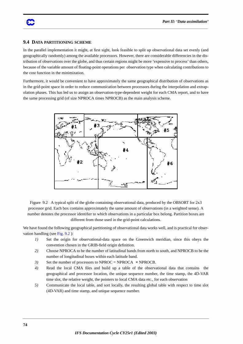
Part II: ‘Data assimilation’
(and
the dis-
others,
ions to
ions as
extrap-
to have
x3
se). A
s are
bser-
s the
e the
the
D-VAR
slot
9.4 DATA PARTITIONING SCHEME
In the parallel implementation it might, at first sight, look feasible to split up observational data set evenly
geographically randomly) among the available processors. However, there are considerable differencies in
tribution of observations over the globe, and thus certain regions might be more ‘expensive to process’ than
because of the variable amount of floating-point operations per observation type when calculating contribut
the cost function in the minimization.
Furthermore, it would be convenient to have approximately the same geographical distribution of observat
in the grid-point space in order to reduce communication between processors during the interpolation and
olation phases. This has led us to assign an observation-type-dependent weight for each CMA report, and
the same processing grid (of size NPROCA times NPROCB) as the main analysis scheme.
Figure 9.2 A typical split of the globe containing observational data, produced by the OBSORT for 2
processor grid. Each box contains approximately the same amount of observations (in a weighted sen
number denotes the processor identifier to which observations in a particular box belong. Partition boxe
different from those used in the grid-point calculations.
We have found the following geographical partitioning of observational data works well, and is practical for o
vation handling (seeFig. 9.2):
1) Set the origin for observational-data space on the Greenwich meridian, since this obey
convention chosen in the GRIB-field origin definition.
2) Choose NPROCA to be the number of latitudinal bands from north to south, and NPROCB to b
number of longitudinal boxes within each latitude band.
3) Set the number of processors to NPROC = NPROCA× NPROCB.
4) Read the local CMA files and build up a table of the observational data that contains
geographical and processor location, the unique sequence number, the time stamp, the 4
time slot, the relative weight, the pointers to local CMA data etc., for each observation
5) Communicate the local table, and sort locally, the resulting global table with respect to time
(4D-VAR) and time stamp, and unique sequence number.
74
IFS Documentation Cycle CY25r1 (Edited 2003)
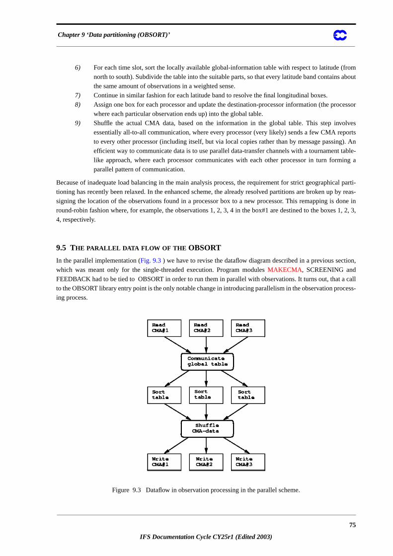
Chapter 9 ‘Data partitioning (OBSORT)’
rom
about
cessor
lves
orts
g). An
table-
ing a
al parti-
by reas-
one in
1, 2, 3,
ion,
call
cess-
6) For each time slot, sort the locally available global-information table with respect to latitude (f
north to south). Subdivide the table into the suitable parts, so that every latitude band contains
the same amount of observations in a weighted sense.
7) Continue in similar fashion for each latitude band to resolve the final longitudinal boxes.
8) Assign one box for each processor and update the destination-processor information (the pro
where each particular observation ends up) into the global table.
9) Shuffle the actual CMA data, based on the information in the global table. This step invo
essentially all-to-all communication, where every processor (very likely) sends a few CMA rep
to every other processor (including itself, but via local copies rather than by message passin
efficient way to communicate data is to use parallel data-transfer channels with a tournament
like approach, where each processor communicates with each other processor in turn form
parallel pattern of communication.
Because of inadequate load balancing in the main analysis process, the requirement for strict geographic
tioning has recently been relaxed. In the enhanced scheme, the already resolved partitions are broken up
signing the location of the observations found in a processor box to a new processor. This remapping is d
round-robin fashion where, for example, the observations 1, 2, 3, 4 in the box#1 are destined to the boxes
4, respectively.
9.5 THE PARALLEL DATA FLOW OF THE OBSORT
In the parallel implementation (Fig. 9.3) we have to revise the dataflow diagram described in a previous sect
which was meant only for the single-threaded execution. Program modulesMAKECMA , SCREENING and
FEEDBACK had to be tied to OBSORT in order to run them in parallel with observations. It turns out, that a
to the OBSORT library entry point is the only notable change in introducing parallelism in the observation pro
ing process.
Figure 9.3 Dataflow in observation processing in the parallel scheme.
75
IFS Documentation Cycle CY25r1 (Edited 2003)
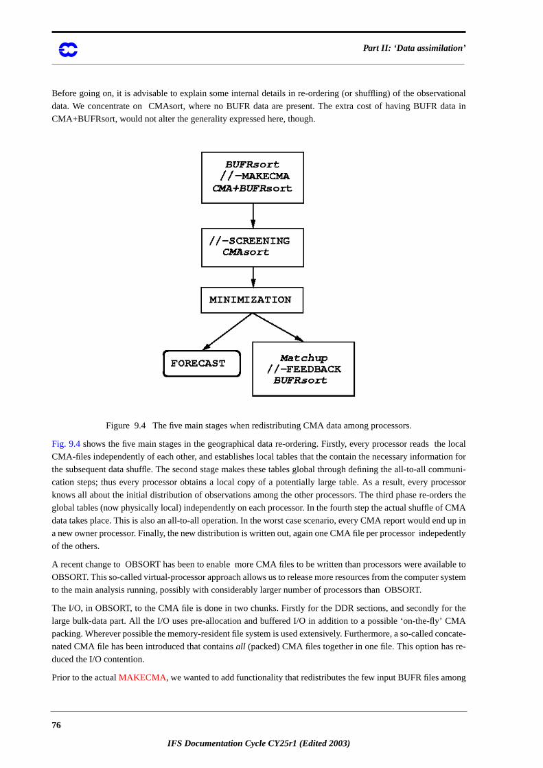
Part II: ‘Data assimilation’
tional
data in
e local
tion for
mmuni-
cessor
ers the
f CMA
d up in
dently
lable to
r system
r the
MA
oncate-
-
ng
Before going on, it is advisable to explain some internal details in re-ordering (or shuffling) of the observa
data. We concentrate on CMAsort, where no BUFR data are present. The extra cost of having BUFR
CMA+BUFRsort, would not alter the generality expressed here, though.
Figure 9.4 The five main stages when redistributing CMA data among processors.
Fig. 9.4shows the five main stages in the geographical data re-ordering. Firstly, every processor reads th
CMA-files independently of each other, and establishes local tables that the contain the necessary informa
the subsequent data shuffle. The second stage makes these tables global through defining the all-to-all co
cation steps; thus every processor obtains a local copy of a potentially large table. As a result, every pro
knows all about the initial distribution of observations among the other processors. The third phase re-ord
global tables (now physically local) independently on each processor. In the fourth step the actual shuffle o
data takes place. This is also an all-to-all operation. In the worst case scenario, every CMA report would en
a new owner processor. Finally, the new distribution is written out, again one CMA file per processor indepe
of the others.
A recent change to OBSORT has been to enable more CMA files to be written than processors were avai
OBSORT. This so-called virtual-processor approach allows us to release more resources from the compute
to the main analysis running, possibly with considerably larger number of processors than OBSORT.
The I/O, in OBSORT, to the CMA file is done in two chunks. Firstly for the DDR sections, and secondly fo
large bulk-data part. All the I/O uses pre-allocation and buffered I/O in addition to a possible ‘on-the-fly’ C
packing. Wherever possible the memory-resident file system is used extensively. Furthermore, a so-called c
nated CMA file has been introduced that containsall (packed) CMA files together in one file. This option has re
duced the I/O contention.
Prior to the actualMAKECMA , we wanted to add functionality that redistributes the few input BUFR files amo
76
IFS Documentation Cycle CY25r1 (Edited 2003)

Chapter 9 ‘Data partitioning (OBSORT)’
CMA,
proc-
n only
ge, an
proper
g ex-
of the
a
nter-
for the
CMA-
its data
ssors
w geo-
a final
with a
n types,
spond-
P clus-
eck the
ocessor
e OB-
e a few
ts as-
be as-
k in a
for-
data
to the
UFR-
-
the
eport
the available processors. Despite an extra step, it boosts overall execution performance of the parallel MAKE
since all processors—not only the first few—will enter into the BUFR data decoding phase. Currently each
essor tries to read in one or more BUFR files in a cyclic fashion. If there were fewer files than processors, the
the few first processors would get a single file; others would remain idle for a while. For each BUFR messa
artificial latitude and longitude is assigned. Also, the basic contents of a BUFR message is checked to get a
weight assigned. After this, the BUFR data can be partitioned in a manner of the ‘geographical’ re-orderin
plained earlier. Despite the tricks involved, this method gives good results and offers nearly maximal re-use
existing source code in OBSORT.
After receiving re-distributed BUFR data,MAKECMA continues to perform its decoding functions, but now in
fully parallel mode. Every MAKECMA process(or) unpacks and writes both a new CMA report and the cou
part BUFR message to a temporary file, one by one. However, the geographical ordering is not optimal
screening purposes. Therefore, the OBSORT needs to be consulted and a CMA-data shuffle followed by a
driven BUFR sort (i.e. CMA+BUFRsort) will be performed as a final substep in MAKECMA.
The screening proceeds in parallel mode by reading local ECMA files, one per processor, and performing
validation functions. Once the resulting CCMA data set is ready, it may occur that in some of the proce
CCMA data has almost vanished due to different kinds of rejections. Therefore, it is necessary to create ne
graphical distribution of observational data, now applied to the CCMA data. The new reordering is done as
step in the screening.
There is a special function present in the OBSORT for post-adjustment of clustered data. It was found that
different number of processors more data got rejected in one case than in another one. Certain observatio
like AIREPs, tended to cluster around partitions’ boundaries. In the first case, a processor owned all the corre
ing observations, since there were no partition boundaries in the neighbourhood; in the second case an AIRE
ter got effectively split among two adjacent processors. For reproducibility reasons, it was necessary to ch
existence of such clusters and to move the clustered observations completely into the lowest numbered pr
around the processors’ boundary
For a better parallel performance in the minimization it is crucial to obtain a good load balance. Therefore, th
SORT’s unique feature that assigns weights for each observation report plays an important role. There ar
built-in weight functions in OBSORT. Depending on the contents of the observation, a different weight ge
signed. The weight functions are controlled by an external input file, where separate weight coefficients can
signed for each observation type.
Finally, it was soon clear, thatMATCHUP could be integrated inthe FEEDBACK. As a resultMATCHUP is per-
formed quickly as the first parallel task in FEEDBACK. The updated local ECMA data is then passed bac
form of CMA array to the actual FEEDBACK which encodes information back to a highly compressed BUFR
mat. Furthermore, the FEEDBACK benefits also from OBSORT’s built-in feature to collect BUFR (or CMA)
into a single processor. This way we were able to get from the final, but still distributed, BUFR data back
non-distributed and ready-to-archive BUFR data in a rather elegant manner. And the fact that the original B
message order was not necessary (or even possible ?) to be preserved, has simplified the programming.
To accomodate the virtual-processor approach, a recent change toMATCHUP has been introduced to perform so
called virtual MATCHUP (or VMATCHUP) prior to the genuine MATCHUP. This option enables us to bring
full set of ECMA files used in the main analysis back to fewer ECMA files, and to preserve the same CMA r
order as in the BUFR message counterparts after MAKECMA.
77
IFS Documentation Cycle CY25r1 (Edited 2003)

Part II: ‘Data assimilation’
9.6 OBSORTCALLING TREE• LIB_OBSORT
• SWAP_FWD
• INIT_COMMON
• SUNUMC
• SETCOMBU
• SUBUOCTP
• SETBUFR
• BUPRQ
• SETCOMCM
• SUCMOCTP
• SUCMA
• CHECK_NAMELIST
• BUFRSORT
• EXPAND_STRING
• DUMP_NAMELIST
• PRECHECK
• PRECHECK_CMA_ARRAY
• SYNC_TIMESLOT_DATA
• GLOBAL
• INIT_COMMON
• GEN_TIMESLOT_DATA
• UPDCAL2
• REF_TIME
• PRECHECK_CMA
• CMA_ATTACH
• CMA_INFO
• CMA_GET_DDRS
• SYNC_TIMESLOT_DATA
• CMA_DETACH
• PRECHECK_BUFR_ARRAY
• UTIL_NUMPROD_ARRAY
• PRECHECK_BUFR
• OLDBUFR_OPEN
• UTIL_NUMPROD
• OLDBUFR_CLOSE
• GLOBAL
• READ_BUFR
• UTIL_PRODLENGTH
• OLDBUFR_OPEN
• OLDBUFR_READ
• OLDBUFR_CLOSE
• GLOBAL
• MAKESEQNO_OBSORT
• PRECHECK
• FILL_SEQNOLIST
• READ_BUFR
78
IFS Documentation Cycle CY25r1 (Edited 2003)
Chapter 9 ‘Data partitioning (OBSORT)’
• CRACK_BUFR_HDR
• BUS012
• BUFRSORT_PREPARE
• CRACK_BUFR_HDR
• OBS_SORT
• COLLECT
• KEYSORT
• REF_TIME
• CHECK_DUPLICATES
• GLOBE_SPLIT
• KEYSORT
• MERGE_CLUSTERS
• BUFR_TRAFFIC_INFO
• IFS_WRITE
• GLOBAL
• .BUFR_SHUFFLE
• SETUP_COMM_DATA
• BUFR_COPY_BUFFER
• WRITE_BUFR
• OLDBUFR_OPEN
• UTIL_ALLOC_IOBUF
• OLDBUFR_WRITE
• OLDBUFR_CLOSE
• BUFR_FORM_EXPLIST
• GEN_TIMESLOT_DATA
• MAPSORT
• EXPAND_STRING
• DUMP_NAMELIST
• PRECHECK
• READ_CMA
• CMA_ATTACH
• CMA_GET_DDRS
• . CMA_BIN_INFO
• CMA_READ
• CMA_CLOSE
• GLOBAL
• REF_TIME
• SORT_PREPARE
• REF_TIME
• GLOBAL
• OBS_SORT
• VMAPSORT
• EXPAND_STRING
• . VCMA_TRAFFIC_INFO
• GLOBAL
• IFS_WRITE
• OPTIMAL_MSGLEN
79
IFS Documentation Cycle CY25r1 (Edited 2003)

Part II: ‘Data assimilation’
• UTIL_IGETENV
• GLOBAL
• VCMA_SHUFFLE
• SETUP_COMM_DATA
• DUMP_INFO
• CMA_COPY_BUFFER
• GLOBAL
• WRITE_OBSMAP
• CMA_STAT
• CMA_OPEN
• DATE_AND_TIME
• CMA_WRITEI
• CMA_CLOSE
• UPDATE_DDR
• GLOBAL
• DATE_AND_TIME
• ADD_SATELLITE
• . REF_TIME
• WRITE_CMA
• CMA_GET_CONCAT_BYNAME
• CMA_OPEN
• CMA_BIN_INFO
• CMA_IS_PACKED
• GLOBAL
• CMA2PCMA
• CMA_INFO
• OPTIMAL_MSGLEN
• COMM_WRITE
• CMA_WRITE
• CMA_CLOSE
• CMA_TRAFFIC_INFO
• GLOBAL
• IFS_WRITE
• OPTIMAL_MSGLEN
• CMA_SHUFFLE
• SETUP_COMM_DATA
• CMA_COPY_BUFFER
• UPDATE_DDR
• WRITE_CMA
• READ_BUFR
• BUFR_PTRLEN_UPDATE
• COLLECT
• KEYSORT
• BUFR_TRAFFIC_INFO
• BUFR_SHUFFLE
• WRITE_BUFR
• CMA_GET_CONCAT_BYNAME
80
IFS Documentation Cycle CY25r1 (Edited 2003)
Chapter 9 ‘Data partitioning (OBSORT)’
• EXPAND_STRING
• MATCHUP
• EXPAND_STRING
• DUMP_NAMELIST
• PRECHECK
• READ_CMA
• MATCHUP_PREPARE
• OBS_MATCHUP
• COLLECT
• . KEYSORT
• CHECK_DUPLICATES
• . KEYSEARCH
• CMA_TRAFFIC_INFO
• OPTIMAL_MSGLEN
• CMA_SHUFFLE
• MATCHUP_PERFORM
• KEYSEARCH
• MATCHUP_REPORT
• UPDATE_DDR
• WRITE_CMA
• VMATCHUP
• EXPAND_STRING
• DUMP_NAMELIST
• READ_OBSMAP
• CMA_STAT
• CMA_OPEN
• . CMA_READI
• DISTR
• CMA_DETACH
• CMA_ATTACH
• CMA_CLOSE
• DISTR_OBS
• GLOBAL
• COLLECT
• PRECHECK
• READ_CMA
• VMATCHUP_PREPARE
• COLLECT
• KEYSORT
• VMATCHUP_TRAFFIC_INFO
• GLOBAL
• OPTIMAL_MSGLEN
• XCMA_SHUFFLE
• SETUP_COMM_DATA
• UPDATE_DDR
• WRITE_CMA
• SWAP_BWD
81
IFS Documentation Cycle CY25r1 (Edited 2003)
Part II: ‘Data assimilation’
82
IFS Documentation Cycle CY25r1 (Edited 2003)

IFS Documentation Cycle CY25r1
Part II: D ATA ASSIMILATION
CHAPTER 10 Observation screening
Table of contents
10.1 Introduction
10.2 The structure of the observation screening
10.2.1 The incoming observations
10.2.2 The screening run
10.2.3 General rationale of the observation screening
10.2.4 3D- versus 4D-Var screening
10.3 The independent observation screening decisions
10.3.1 Preliminary check of observations
10.3.2 Blacklisting
10.3.3 Background quality control
10.4 Screening of satellite radiances
10.4.1 General
10.4.2 Input
10.4.3 Bias correction
10.4.4 Quality control
10.4.5 Retrieval
10.4.6 SSM/I radiances
10.4.7 Geostationary clear-sky radiances
10.5 Scatterometer processing
10.5.1 Introduction
10.5.2 Background and general Scatterometer geometry
10.5.3 Location of scatterometer data in the ECMWF archives
10.5.4 ESA scatterometer (ERS-1 and ERS-2) processing
10.5.5 NASA scatterometer (NSCAT) processing
10.5.6 NASA “QUIK” scatterometer (QuikSCAT) processing
10.6 The dependent observation screening decisions
10.6.1 Update of the observations
10.6.2 Global time–location arrays
83
IFS Documentationn Cycle CY25r1 (Edited 2003)

Part II: ‘Data assimilation’
ral de-
lean
f dupli-
ionally
t the old
updated
ainder.
nverted
k for the
tem-
a set
s entails
d wet
et (ec-
at the
obser-
e exact
parate
t (high
l the
as these
10.6.3 Vertical consistency of multilevel reports
10.6.4 Removal of duplicated reports
10.6.5 Redundancy check
10.6.6 Thinning
10.6.7 A summary of the current use of observations
10.6.8 Compression of the ODB
10.7 A massively-parallel computing environment
10.1 INTRODUCTION
This chapter describes the observation screening in the ECMWF 3D/4D-Var data assimilation. A more gene
scription can be found inJärvinenand Undén(1997). The purpose of the observation screening is to select a c
array of observations to be used in the data assimilation. This selection involves quality checks, removal o
cated observations, thinning of their resolution etc.. The new selection algorithm was implemented operat
in September 1996 and was designed to reproduce (to a large extent) the selection of observations tha
screening of the ECMWF OI analysis code used to make (Lönnberg and Shaw, 1985 and 1987;Lönnberg, 1989).
This chapter was prepared in September 1997 by Heikki Järvinen, Roger Saunders and Didier Lemeur, and
in February 1999 by Roger Saunders for TOVS processing, by Elias Holm and Francois Bouttier for the rem
10.2 THE STRUCTURE OF THE OBSERVATION SCREENING
10.2.1 The incoming observations
Before the first trajectory integration, the observations are extracted from a data base of observations co
from the BUFR archive to a set of CMA files (by programsobsproc andobsort described in the ‘observation’ part
of the documentation). These data have already undergone some rudimentary quality control, e.g. a chec
observation format and position, for the climatological and hydrostatic limits, as well as for the internal and
poral consistency (Norris, 1990). The so-called RDB (Report Data Base) flag is assigned at this stage. Then
of observation files suitable for assimilation is created in a separate observation preprocessing module. Thi
format conversions, changes of some observed variables (like calculation of relative humidity from dry an
bulb temperatures), as well as assignment of observation error statistics. The resulting ‘extended’ CMA file s
ma.# ; # = processor id) contains all the observational information from the six-hour data window available
cut-off time, and is an input for the IFS. The observation screening then selects the best quality and unique
vations, preferably close to the middle of the data window because the background is not interpolated to th
time of the observation. Unlike the OI, the 3D- and 4D-Var data assimilation is global and, therefore, no se
data selection for analysis boxes is needed.
10.2.2 The screening run
The ECMWF 3D/4D-Var data assimilation system makes use of an incremental minimization scheme (Courtieret
al. 1994 and 1997) to reduce the computational cost. The variational data assimilation starts with the firs
resolution) trajectory run (CONF = 2, LSCREEN = .TRUE.). During this run the model counterparts for al
observations are calculated through the nonlinear observation operators (controlled by taskob). As soon
84
IFS Documentation Cycle CY25r1 (Edited 2003)
Chapter 10 ‘Observation screening’
screen-
riables
d’ ob-
lity con-
. The
ent min-
varia-
ept in
ssary in
d quality
other
OVS
serva-
ill be
window
have
ar as-
indow,
with the
the time
r the
times-
on can
k in the
nction
e of the
nd ver-
background departures are available for observations, the screening can be performed. For the observation
ing, the background errors (errgrib - file) are interpolated to the observation locations for the observed va
(sufger).
Technically, the final result of the observation screening is a pair of observation arrays. The original ‘extende
servation array now contains observations complemented by the background departures, together with qua
trol information for most of the observations. This array is stored for later feedback (ecma.# - set of files)
compressed observation array is a subset of the original array of observations, and is passed for the subsequ
imization job. The compressed array (ccma.# - set of files) contains only the observations to be used in the
tional assimilation. Memory wise, the first trajectory run is a demanding one as all the observations are k
memory. Prior to the screening the model fields are deallocated (dealmod) as most of the information nece
the screening is stored in the observation data base (ODB).
10.2.3 General rationale of the observation screening
The general logic in the 3D/4D-Var observation screening algorithm is to make theindependentdecisions first, i.e.
the ones that do not depend on any other observations or decisions (decis). One example is the backgroun
control for one observed variable. These can be carried out in any order without affecting the result of any
independent decision. The rest of the decisions are considered as mutuallydependenton other observations or de-
cisions, and they are taken next, following a certain logical order. For instance, the horizontal thinning of T
reports is only performed for the subset of reports that passed the background quality control. Finally, the ob
tion array is compressed (compres) for the minimization in such a way that it only contains the data that w
used.
10.2.4 3D- versus 4D-Var screening
In the 3D-Var assimilation system, the observations processed have been gathered over a 6-hour long time
(from 3 hours before to 3 hours after the nominal analysis time) ; all the screening is performed as if they
actually been performed simultaneously at the central analysis time. In the early implementation of the 4D-V
similation system, the same processing called 3D-screening was applied over the 6-hour long 4D-Var time w
which resulted in essentially the same screening decisions as in 3D-Var, except that the model comparison
observation was performed at almost the appropriate time with no more than a 30-minute approximation.
In summer 1997, a new screening procedure called 4D-screening was implemented that took into account
dimension of the observations. The time window was divided in timeslots of typically 1-hour length (30mn fo
first and the last time slot). The 3D-screening algorithm was then applied separately to observations in each
lot. This allowed more data to be used by 4D-Var, for instance, all messages from an hourly reporting stati
now be used, whereas only one (closest to central time) would have been allowed by the redundancy chec
3D-screening. The 4D-screening behaviour is activated by switch LSCRE4D ; it is meant to be used in conju
with time correlation of observation errors where appropriate, as explained inJärvinenet al(1999) and in the chap-
ter on conventional obs error constraints.
10.3 THE INDEPENDENT OBSERVATION SCREENING DECISIONS
10.3.1 Preliminary check of observations
The observation screening begins with a preliminary check of the completeness of the reports (prech). Non
following values should be missing from a report: observed value, background departure, observation error a
85
IFS Documentation Cycle CY25r1 (Edited 2003)
Part II: ‘Data assimilation’
d pilot
eight) is
tial ob-
d as a
ht dif-
ialized
IFS
ila-
s, ver-
through
ing too
ith the
cklist
manner
ound
he as-
ted as
kground
given
idered
For the
(FG-
0 for
ctively
the
JO. For
tical coordinate of observation. Also a check for a missing station altitude is performed for synop, temp an
reports. The reporting practice for synop and temp mass observations (surface pressure and geopotential h
checked (repra), as explained in the appendix. At this stage also, the observation error for synop geopoten
servations is inflated if the reported level is far from the true station level (addoer). The inflation is define
proportion of the difference between the reported level and the true station altitude by adding 2% of the heig
ference to the observation error.
10.3.2 Blacklisting
Next, the observations are scanned through for blacklisting. At the set-up stage the blacklist interface is init
(blinit) to the external blacklist library (libbl95.a). The interface between the IFS and the black-list is in the
routine BLACK. The blacklist itself consists formally of two parts. Firstly, the selection of variables for assim
tion is done using the data selection part of the blacklist file. This controls which observation types, variable
tical ranges etc. will be selected for the assimilation. Some more complicated decisions are also performed
the data selection file; for instance, an orographic rejection limit is applied in the case of the observation be
deep inside the model orography. This part of the blacklist also provides a handy tool for experimentation w
observing system, as well as with the assimilation system itself. Secondly, a normal monthly monitoring bla
is applied for discarding the stations that have recently been reporting in an excessively noisy or biased
compared with the ECMWF background field. A full documentation of the new blacklisting mechanism is f
in Järvinen et al. (1996).
10.3.3 Background quality control
The background quality control (FIRST) is performed for all the variables that are intended to be used in t
similation. The procedure is as follows. The variance of the background departure can be estima
a sum of observation and background error variances , assuming that the observation and the bac
errors are uncorrelated. After normalizing with , the estimate of variance for the normalized departure is
by . In the background quality control, the square of the normalized background departure is cons
as suspect when it exceeds its expected variance more than by a predefined multiple (FGCHK, SUFGLIM).
wind observations, the background quality control is performed simultaneously for both wind components
WND). In practice, there is an associated background quality-control flag with four possible values, namely
a correct, 1 for a probably correct, 2 for a probably incorrect and 3 for an incorrect observation, respe
(SUSCRE0).Table 10.1gives the predefined limits for the background quality control in terms of multiples of
expected variance of the normalized background departure. These values can be changed in namelist NAM
satob winds the background error limits are modified as explained inAppendix A.
TABLE 10.1 THE PREDEFINED LIMITS FOR THE BACKGROUND QUALITY CONTROL, GIVEN IN TERMS OF MULTIPLES
OF THE EXPECTED VARIANCE OF THE NORMALIZED BACKGROUND DEPARTURE.
Variable Flag 1 Flag 2 Flag 3
u, v 9.00 16.00 25.00
z, ps 12.25 25.00 36.00
dz x x x
T 9.00 16.00 25.00
rh, q 9.00 16.00 25.00
y H xb( )–
σo2 σb
2+
σb
1 σo2 σb
2⁄+
86
IFS Documentation Cycle CY25r1 (Edited 2003)
Chapter 10 ‘Observation screening’
limits
ind
If the
back-
r high
h to
docu-
module
evals
and
del
location
l polar
tch IS
ribed
ar are
is set
ed, an
set
m-
AD-
13.25
-
-5 be-
a, and
There is also a background quality control for the observed wind direction (FGWIND). The predefined error
of 60o, 90o and 120o apply for flag values 1, 2 and 3, respectively. The background quality control for the w
direction is applied only above 700 hPa for upper-air observations for wind speeds larger than .
wind-direction background quality-control flag has been set to a value that is greater than or equal to 2, the
ground quality-control flag for the wind observations is increased by 1. For scatterometer winds, a test fo
wind speeds and cold SST is applied in the IFS routine FGWIND.
10.4 SCREENING OF SATELLITE RADIANCES
This section describes the use of RTOVS, valid in April 1999. At the time of writing it was planned to switc
using 1-C radiances for which the processing is rather different; it is described in a separate chapter of the
mentation.
10.4.1 General
The radiances from the RTOVS 120 km BUFR data received from NESDIS are preprocessed in a dedicated
which performs several functions to allow the assimilation of TOVS radiances in 4D-Var (the NESDIS retri
are not used in 4D-Var, but are only monitored with the background profiles). This module is called ADVAR
is part of the TOVSCODE library (libtovscode.a). ADVAR is called for each TOVS observation with the mo
background temperature, specific-humidity and ozone profiles, and surface parameters interpolated to the
of the observations. For each analysis cycle there are typically 22,000 TOVS observations in total, for a dua
orbiter system. ADVAR performs the following functions described below, dependent on the setting of a swi
which determines the mode of operation of ADVAR
. In the screening pass ADVAR is called twice by TOVCLR, once with IS set to 1 (when all the operations desc
below are performed) and once with IS set to –1 (when only the high resolution radiance departures for 4D-V
computed). When IS is set to –1 the profile extrapolation and 1D-Var retrieval is not performed. Finally if IS
to 0 then the background radiances are computed from the profiles, but the 1D-Var retrieval is not perform
option only used for offline tests. Several input files are required for ADVAR which are listed in Table 0.2. A
up routine for ADVAR (SUADVAR) is called within the IFS by SURAD to open the necessary files and fill co
mon arrays for ADVAR and the fast radiative transfer model RTTOV-5. The various operations performed by
VAR are described below. The full scientific description of ADVAR is described in the paper byEyreet. al.(1993).
10.4.2 Input
The fast radiative-transfer model RTTOV-5 for TOVS radiances requires an input profile of 40 levels from 10
to 0.1 hPa. RTTOV-5 has been described in detail bySaunders et al.(1999). The original forecast model tempera
ture, specific-humidity and ozone profiles are interpolated onto the fixed pressure levels required by RTTOV
fore they are input to ADVAR. For the 31 level model, the background profiles are only available up to 10 hP
Flag values are denoted by 1 for a probably correct, 2 for a probablyincorrect and 3 for an incorrect observation. The variables aredenoted by u and v for wind components, z for geopotential height,ps for surface pressure, dz for thickness, T for temperature, rhfor relative humidity and q for specific humidity, respectively.
TABLE 10.1 THE PREDEFINED LIMITS FOR THE BACKGROUND QUALITY CONTROL, GIVEN IN TERMS OF MULTIPLES
OF THE EXPECTED VARIANCE OF THE NORMALIZED BACKGROUND DEPARTURE.
Variable Flag 1 Flag 2 Flag 3
15 m s1–
87
IFS Documentation Cycle CY25r1 (Edited 2003)

Part II: ‘Data assimilation’
a, and a
med for
extrap-
ute the
chan-
so an extrapolation has to be performed up to 0.1 hPa for temperature using the NESDIS retrievals to 1 hP
simple extrapolation based on model atmospheres above this level. Climatological mean profiles are assu
water vapour and ozone. For the 50- and 60-level versions of the model with levels in the stratosphere this
olation is not necessary. Once the full profile is defined and checked (see below) RTTOV-5 is called to comp
background radiances from the background profiles. Background radiances are computed for all the TOVS
nels listed inTable 10.2, but only a subset of the channels are subsequently used in the 1D-Var retrieval.
TABLE 10.2 TOVSCHANNEL USAGE AND (O+F) ERRORS ASSUMED IN1D-VAR (THE ERRORS USED IN4D-VAR
ARE INFLATED BY 50%)
Channel Number 1/4D-Var usageClear(K)
Cloudy(K)
Land/mixed(K)
Sea-ice(K)
1 All/global 1.40 1.40 1.40 1.40
2 All/global 0.35 0.35 0.35 0.35
3 All/global 0.30 0.30 0.30 0.30
4 Clear/sea/global 0.20 0.20 0.20
5 Clear/sea/global 0.30 0.30 0.30
6 Clear/sea/global 0.40 0.80 0.80
7 Clear/sea 0.60 1.20
8 Clear/sea 1.00 2.00
9 FG only
10 Clear/sea 0.80 1.60
11 Clear/global 1.10 1.10 1.10
12 Clear/global 1.50 1.50 1.50
13 Clear/sea 0.50 1.00
14 Clear/sea 0.35 0.70
15 Clear/sea 0.30 0.60
16 FG only
17 FG only
18 FG only
19 FG only
21 QC check
22 All/sea* 0.30 0.30 1.00
23 All/global* 0.22 0.22 0.22 0.22
24 All/global 0.25 0.25 0.25 0.25
25 All/global 0.60 0.60 0.60 0.60
26 All/global 1.00 1.00 1.00 1.00
27 All/global 1.80 1.80 1.80 1.80
*Cloudy data not used in tropics
88
IFS Documentation Cycle CY25r1 (Edited 2003)

Chapter 10 ‘Observation screening’
TOVS
ce
rapidly
tellites,
s a flag
values
L
the
ithin
and are
n-zero
ss than
e they
set for
10.4.3 Bias correction
The next step is to apply the bias correction to the NESDIS radiances. The details of the bias correction for
radiances is given inEyre(1992) andHarris (1997). An update to the bias correction coefficients is performed on
a month on the past two to four weeks of radiance-departure statistics, the exact period depending on how
the biases have changed during the period. The bias-correction coefficients are stored in a file for all of the sa
and this is used in ADVAR. The bias correction code is in the BIASCOR subdirectory of TOVSCODE.
10.4.4 Quality control
Several quality checks are then applied to the measured and background radiances, and ADVAR return
(IFAIL); this is zero if all the checks are passed, but is set to a specific value if a problem is detected. The
for IFAIL and their meaning are given inTable 10.3. The radiances or retrievals are only used in 4D-Var if IFAI
is zero. The gross checks applied are:
(i) Check that the background profile vector is within realistic limits (e.g. temperature is within
range 150–350 K, specific humidity is positive and not supersaturated, ozone is w
climatological extremes). ADVAR terminates with a severe error flag if this test fails.
(ii) The measured and background brightness temperatures are present for all required channels
within the range 150–350 K.
A series of more critical tests are then applied where ADVAR continues even if the test fails but returns a no
IFAIL value.
(i) Gross background check (i.e. the measured radiance departures from the background are le
20 K).
(ii) The background temperature, specific humidity and ozone profiles are checked to make sur
are close to, or within, the range encompassed by the diverse 32 (or 35 for ozone) profile data
which the RTTOV is valid.
TABLE 10.3 DEFINITION OF 1D-VAR FAILURE FLAGS AND TYPICAL RATES IN THEIFS.
IFAIL Typical % Comment
0 80% Retrieval OK
nn 1.0% Measurement cost too high for channelnn
55 17% At edge of scan, otherwise OK
66 0% Failed stability check (not applied)
99 0.5% Minimization failed to converge
100 1.0% Failed window channel cloud test
5nn 0.1% Channelnn failed fine background check
6nn 0.3% Channelnn failed gross background check
7nn 0% Bad background radiance for channel nn
887 0.3% background profile outsideRTTOV limits
888 0% background profile corrupt
9nn 0% Radiances for channel nn corrupt
999 0% No valid scan or valid satid or bias coeffs
89
IFS Documentation Cycle CY25r1 (Edited 2003)

Part II: ‘Data assimilation’
greater
ance
Over
d in 4D-
ll valid
etails
ed
cloudy
n
4D-Var.
tions
han 0.4
defined
ground
ters also
layer-
trievals.
ofiles
(iii) A fine background check where the square of the radiance departures are flagged if they are
than (see below for definitions).
(iv) A check for cloud contamination for the HIRS channels is included by checking that the radi
departure for HIRS channel 8 is inside the range –4 to +8 K over the sea and south of 20˚N.
land the thresholds are brighter north of 20˚N. IFAIL is set to 100 if outside this range.
(v) Radiances at the two extreme edge positions of the swath are flagged at present and not use
Var.
(vi) Checks are also made that the bias-correction coefficients, satellite id, and scan position are a
before proceeding.
10.4.5 Retrieval
The main task for ADVAR is to perform a 1D-Var retrieval of temperature, water vapour and ozone profiles. D
on the theory of 1D-Var retrieval are described byEyreet al. (1993), and so only the technical details describ
here are concerned with the implementation at ECMWF. Each radiance profile is assigned to be clear, partly
or cloudy by NESDIS, and different TOVS channels and observation errors are used for each type as listed iTable
10.2. The files defining the channel selection and observation plus forward model error(O+F) covariances are giv-
en inTable 10.4and no interchannel correlations are assumed (i.e. a diagonal matrix). The(O+F) errors specified
here are subsequently used in 4D-Var, but are inflated by 50%. The background-error covariancesB for all 43 levels
are also specified in a file, and for temperature are close to the global-mean background errors assumed in
For specific humidity the background errors assumed in 1D-Var follow the same formulation as in 4D-Var (Rabier
et al. 1997) and the correlations are the same as in 4D-Var.
The minimization of the cost function is performed using the method of Newtonian iteration, and up to 5 itera
are allowed before the minimization fails. Convergence is obtained when the profile departures are less t
times at every level. If the cost function of the observed radiance in any of the channels exceeds a pre
threshold then a flag is set indicating an inconsistent set of radiances. The output of 1D-Var includes back
and retrieved temperature, water-vapour and ozone profiles, together with several retrieved surface parame
included in the 1D-Var control vector. The retrieved profiles are output both on the 43 levels and as virtual
mean temperatures on 15 levels and layer-mean column water vapour on 3 levels to match the NESDIS re
A final check on the stability of the retrieved profile is provided in the code, but is not implemented as the pr
are not used in 4D-Var.
TABLE 10.4 FILES REQUIRED BYADVAR
Filename Contents
chanspec.dat Specifies channel usage
rmtberr.dat Specifies radiance observation errors (O+F)
fcbkerr.dat Specifies 1D-Var background error covari-ances (B)
bcor.dat Bias correction coefficients
rt_coef_ieee.dat orrt_coef_fmt.dat
RTTOV coefficients in binary or ascii format.
16 KBK T O F+ +[ ]×
σb
90
IFS Documentation Cycle CY25r1 (Edited 2003)
Chapter 10 ‘Observation screening’
o AD-
cloud
0km.
mmer
rformed
quality
adianc-
lites are
d from
n sys-
n the
to de-
idance
emote
d infor-
eir pe-
, lists
-1 and
, ERS-2,
es in
of scat-
ed into
01. The
CAT
ta have
ometer
10.4.6 SSM/I radiances
SSM/I radiances are also screened in a similar module DVSSMI, which performs a similar set of functions t
VAR B by retrieving the total column water vapour, surface wind speed and cloud liquid-water path. The total
water vapour retrievals have been activated operationally in Spring 1998, with an horizontal thinning to 25
A specialized library,ssmicodeis used for the retrievals. Some documentation can be found inGerardand Saun-
ders (1999). At the time of writing it is envisaged to start using surface wind speed retrievals over sea in su
1999.
10.4.7 Geostationary clear-sky radiances
Geostationary clear-sky radiances (GRAD) follow the same path as level-1C radiances. Data selection is pe
through blacklisting (see Table 10.6 for usage in CY25R1), thinning, and a first-guess and variational data
control check. While water vapour radiances of Meteosat-7 are actively assimilated, water vapour channel r
es from GOES-8 and GOES-10 and the infrared window channel radiances of Meteosat and GOES satel
only passively monitored (water vapour channel radiances of GOES-8 and GOES-10 are actively assimilate
CY25R3 onwards).
10.5 SCATTEROMETER PROCESSING
10.5.1 Introduction
This section describes the flow of ERS, NSCAT, and QuikSCAT scatterometer data through the assimilatio
tem. Many tasks like the thinning of ERS data and the retrieval of 50 km QuikSCAT winds are performed i
module PRESCAT, which, being part of the OBS family, are run before the screening. But it is most natural
scribe the whole processing step here. This section provides a working knowledge of the software, and gu
on possible modifications and updates. It is not intended to explain the scientific background of microwave r
sensing or scatterometry and assumes some knowledge of these topics (seeStoffelen(1999),Freilich and Dunbar
(1999)).
Besides the introduction, this section is broken into five subsections. The next subsection gives backgroun
mation on scatterometer processing at ECMWF. It includes a brief description of the various instruments, th
riod of functioning and operational assimilation at ECMWF. Besides it provides some history of the software
persons who contributed to the changes and outlines the structure and function of the whole library.Subsection
10.5.3gives concise information on the location of scatterometer data in the ECMWF archives.Subsections
10.5.4–10.5.6describe the line of processing for scatterometers used or currently in use at ECMWF, i.e. ERS
ERS-2, NSCAT and QuikSCAT.
10.5.2 Background and general Scatterometer geometry
ESA’s ERS-1 scatterometer was launched in July 1991 and stopped operating in June 2000. Its successor
was launched in 1995 and is still working. However, due to the loss of a proper functioning of its gyroscop
January 2001 the yaw attitude control of the spacecraft has deteriorated. This especially affects the quality
terometer data, and as a result, its worldwide distribution was suspended. Data from ERS-2 were introduc
operations at ECMWF in January 1996 and have been used in operations until its suspension in January 20
NSCAT instrument was part of the payload of the ADEOS-I satellite, which was launched in August 1996. NS
data have been available from mid September 1996 until the spacecraft failure on June 30 1997. NSCAT da
never been part of the operational 4-D Var system. The QuikSCAT satellite, carrying the SeaWinds scatter
91
IFS Documentation Cycle CY25r1 (Edited 2003)

Part II: ‘Data assimilation’
anuary
quency,
rface.
r values
. More
assim-
nas on
600 km
50 km.
at Ku-
beam
r 1,400
s. The
can have
in
n and
ooked
oquet,
. Later
tional
.
contains
oal
eral
7, i.e. its
instrument, was launched in June 1999. Its data was introduced in the operational 4-D Var system on 22 J
2002 and has been assimilated since that date.
The scatterometers aboard the ERS-1 and ERS-2 satellites are of identical design. Operating at C-band fre
three antennas at the right-hand side from the flight direction ( , and ) illuminate the ocean su
Inside the 450 km wide swath, 19 nodes define a 25 km product. For each such node, average backscatte
for the three beams are determined from a 50 km by 50 km footprint, i.e., the 25 km product is over-sampled
detailed information on the ERS scatterometers can be found in Attema (1986), its impact on the ECMWF
ilation system inIsaksen (1997) andIsaksenand Stoffelen (2000).
The NSCAT scatterometer that was part of the payload of the ADEOS-I satellite, consisted of three anten
each side of the spacecraft. It operated at Ku-band frequency, and provided coverage in two simultaneous
wide swaths, separated by a 350 km wide nadir gap. The resolution of the backscatter and wind product was
More detailed information on the NSCAT scatterometer can be found in the appendix ofCheltonet al. (2000), its
impact on the ECMWF assimilation system inLeidneret al. (2003).
The Seawinds scatterometer aboard the QuikSCAT satellite, finally, consists of two rotating beams operating
band frequency with incidence angles w.r.t. the normal of the ocean surface of respectively . Each
provides a fore and an aft measurement. They cover a swath of 1,800 km in diameter, although only the inne
km is illuminated by both beams. The product is determined on a 25 km resolution, defining 76 across node
first eight and last eight nodes contain two backscatter measurements (outer beam only), the other nodes
up to 4 backscatter measurements. More detailed information on the QuikSCAT scatterometer can be foundLei-
dneret al. (2000), its impact on the ECMWF assimilation system inHersbachet al. (2003).
Ad Stoffelen, David Anderson and Ross Hoffman were the first to work on the problem at ECMWF. Stoffele
Anderson worked on quality control (QC) and wind retrieval issues in the OI system of these days. Hoffman l
at assimilation of backscatter information directly in 3D-Var. Once in operations, several others (Herve R
Catherine Gaffard, Didier LeMeur and Lars Isaksen) took turns monitoring and improving the use of the data
Mark Leidner worked on the use of data from NASA scatterometers (NSCAT and QuikSCAT) and the opera
implementation of the assimilation of QuikSCAT data was completed by Hans Hersbach and Lars Isaksen
Source code for scatterometer processing resides in ClearCase under the project name SCAT. The library
the following directories:
• etimesort/ source code for pre-processing ERS data
• module/ shared modules
• qbukey/ source code for adding RDB info to QuikSCAT 50km BUFR
• qfilter/ source code for pre-processing QuikSCAT 25km BUFR
• qretrieve/ source code for SeaWinds wind retrieval
• dcone_qc/source code to perform a global quality control check on QuikSCAT data with the g
to detect instrument anomalies
• qsca_split/source code that allows for the distribution of QuikSCAT pre-processing over sev
processors (not active)
• monitoring/ empty directory in which scatterometer monitor software may reside in future
• test/ empty directory for future test code
NSCAT-specific codes have not been put in ClearCase, because the satellite stopped operating in June 199
data will never be used in operations.
45° 90° 135°
46° 56°
92
IFS Documentation Cycle CY25r1 (Edited 2003)
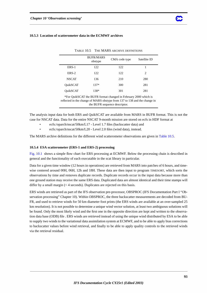
Chapter 10 ‘Observation screening’
t the
ed in
time-
ore than
mps will
t I “Ob-
om BU-
led 25
s will
erva-
e able
ctions
winds
10.5.3 Location of scatterometer data in the ECMWF archives
The analysis input data for both ERS and QuikSCAT are available from MARS in BUFR format. This is no
case for NSCAT data. Data for the entire NSCAT 9-month mission are stored on ecfs in HDF format at
• ecfs:/oparch/nscat/50km/L17 - Level 1.7 files (backscatter data) and
• ecfs:/oparch/nscat/50km/L20 - Level 2.0 files (wind data), instead.
The MARS archive definitions for the different wind scatterometer observations are given inTable 10.5.
10.5.4 ESA scatterometer (ERS-1 and ERS-2) processing
Fig. 10.1 shows a simple flow chart for ERS processing at ECMWF. Below the processing chain is describ
general and the functionality of each executable in the scat library in particular.
Data for a given time window (12 hours in operations) are retrieved from MARS into patches of 6 hours, and
wise centered around 00H, 06H, 12h and 18H. These data are then input to programTIMESORT, which sorts the
observations by time and removes duplicate records. Duplicate records occur in the input data because m
one ground station may receive the same ERS data. Duplicated data are almost identical and their time sta
differ by a small margin (< 4 seconds). Duplicates are rejected on this basis.
ERS winds are retrieved as part of the IFS observation pre-processor, OBSPROC (IFS Documentation Par
servation processing” Chapter 10). Within OBSPROC, the three backscatter measurements are decoded fr
FR, and used to retrieve winds for 50 km diameter foot prints (the ERS winds are available at an over-samp
km resolution). It is not possible to determine a unique wind vector solution, at least two ambiguous solution
be found. Only the most likely wind and the first one in the opposite direction are kept and written to the obs
tion data base (ODB) file . ERS winds are retrieved instead of using the unique wind distributed by ESA to b
to supply two winds to the variational data assimilation system at ECMWF, and to be able to apply bias corre
to backscatter values before wind retrieval, and finally to be able to apply quality controls to the retrieved
via the retrieval residual.
TABLE 10.5 THE MARS ARCHIVE DEFINITIONS
BUFR/MARSobstype
CMA code type Satellite ID
ERS-1 122 122 1
ERS-2 122 122 2
NSCAT 136 210 280
QuikSCAT 137* 300 281
QuikSCAT 138* 301 281
*For QuikSCAT the BUFR format changed in February 2000 which isreflected in the change of MARS obstype from 137 to 138 and the change in
the BUFR sequence descriptor.
93
IFS Documentation Cycle CY25r1 (Edited 2003)

Part II: ‘Data assimilation’
se the
kscatter
along
m 1 to 19
the data
M-
s best at
de 3,
ead of
ements
hat the
ssigned
before
at the
and
Figure 10.1 ERS processing
A horizontal thinning is performed on the 19 x 19 data layout of the ERS scatterometer reports. In that ca
process is defined with respect to the particular measurement geometry of the instrument. Indeed, the bac
data are acquired within individual cells related to a 450 km wide grid with a mesh of 25 km in the across and
track directions. 19 measurement nodes are thus defined across the scatterometer´s swath, numbered fro
as the incidence angle increases, while 19 rows are also considered in the along track direction to gather
in squares of 19 by 19 points. The thinning factor is controlled by LSCATTHI and NTHINSCA in namelist NA
MKCMA. The inner two nodes are skipped (smallest incidence angles) because the scatterometer operate
larger incidence angles. Then, every NTHINSCA node is used (default NTHINSCA = 4 results in use of no
7, 11, 15, and 19) in every NTHINSCA row. The data are thus by default used at a resolution of 100 km inst
the original 25 km sampling distance. This simple way of thinning is preferable because ERS wind measur
typically always are of the same high quality as they are not affected by rain or clouds. It should be noted t
thinning process is actually set up in the observation pre-processing (OBSPROC), but that only a flag is a
at that stage, which is then applied in the screening. In that way all the data are completely pre-processed
assimilation, and the subsequent information kept in the feedback files allows to perform their monitoring
full resolution.
In the IFS, the two retrieved winds are used in an observation cost function with two minima (seepp_obs/HJO).
The function is not quadratic, but depends on the fourth power and root of the product of the departures of
(Stoffelen and Anderson (1997)):
. (10.1)
In the vicinity of each solution, this cost function looks quadratic. The observation errorσ0 is 2 m/s (defined in the
OBSPROCmake_cma/QSCATIN routine).
Quality control decisions made by the IFS screening run are:
uv
J u( )J1J2
J14 J2
4+( )0.25
------------------------------- J1 2, u( ),,u u1 2,– 2
σ02
--------------------------= =
94
IFS Documentation Cycle CY25r1 (Edited 2003)

Chapter 10 ‘Observation screening’
m/s
it
to be
tter
older
lot is
r effec-
the feed-
ack data.
in which
ds
in
n
=
.
C
1
n
r
SCAT
d Quik-
SCAT
• High wind speed check:Data rejected if observed or first guess wind speeds are above 25
(RSCAWLI). Performed byobs_preproc/FGWND
• Sea ice check:Data rejected if sea-ice fraction is higher than 0.01 (RSCATLI) This upper lim
used to be 0.1. However, since CY24R3 it was made more strict because it was found
insufficient to remove all sea-ice contaminated data. Performed byobs_preproc/FGWND
• Global quality control: If the average distance-to-the-cone residual for the backsca
measurements during an observation time slot (30 minutes since CY24R3, and 1 hour for
cycles) for any of the active nodes is above the QC threshold, all ERS data for that time s
blacklisted. This is done by the routineobs_preproc/SCAQC.
There is no background wind check performed on ERS scatterometer data, but data may be de-weighted o
tively removed from the analysis during the minimization in 4D-Var by variational quality control (Andersson and
Järvinen (1999)).
Quality control decisions and departures from background and analyses are appended to each subset in
back BUFR message.
ERS feedback messages have a PRESCAT section sandwiched between the original ERS and the feedb
The PRESCAT section contains outputs about the quality of the winds from the retrieval.
Here are some of the key words and bits to examine in the ERS feedback message (these are in the order
they are encountered in the processing):
• Winds retrieved at ESA: BUFR descriptor 11012 for speed and 11011 for direction win
available in observation part of BUFR file.
• Winds retrieved at ECMWF: BUFR descriptor 11192 for and 11193 for winds retrieved
program OBSPROC.
• Report rejected by thinning if BUFR descriptor 33229 (Report Event Word 2) = 1. QC decisio
made by program OBSPROC in subroutinemake_cma/SCATSIN.
• Background departures x 2 ambiguities:BUFR descriptor 224255 for (‘U - COMPONENT
AT 10 M’) and for (‘V - COMPONENT AT 10 M’). BUFR descriptor 8024 = 33, BUFR
descriptor 33210 = 1, BUFR descriptor 33211 = 1001.
• Report rejected by high wind speed checkif BUFR descriptor 33233 (Report Status Word 1)
16. QC decision made by program IFS in subroutineobs_preproc/FGWND.
• Report rejected if Sea Ice faction too high: BUFR descriptor 33220 (Report Event Word 1) = 12
QC decision made by program IFS in subroutineobs_preproc/FGWND.
• Report rejected if global QC fails: BUFR descriptor 33220 (Report Event Word 1) = 16. Q
decision made by program IFS in subroutineobs_preproc/ERSQC.
• Datum 4D-Var quality control status: BUFR descriptor 33233 (Report Status Word 1) = 1/2/4/8
- active, 2 - passive, 4 - rejected, 8 - blacklisted Datum. 4D-Var variational quality control rejectio
BUFR descriptor 33236 (Datum event Word 1) bit 27 = 1
• Analysis departures x 2 ambiguities:BUFR descriptor 224255 for (‘U - COMPONENT AT 10
M’) and for (‘V - COMPONENT AT 10 M’). BUFR descriptor 8024 = 33, BUFR descripto
33210 = 9, BUFR descriptor 33211 = 999.
10.5.5 NASA scatterometer (NSCAT) processing
NSCAT data has been used experimentally for impact experiments in 4D-Var as well as a surrogate for Quik
data (Ku-band scatterometer as well). The processing is not automatic in IFS , as is the case for ERS an
SCAT. The NSCAT data quality is more consistent compared to ERS and QuikSCAT, because the archived N
u v
uv
uv
95
IFS Documentation Cycle CY25r1 (Edited 2003)

Part II: ‘Data assimilation’
ct Us-
Each
ontact
cribed
is lev-
wever.
tation
an be
cen-
rt of the
defined
e paired
ion. This
tivation
e incre-
data are a re-processed science product, not an “as-is” real-time product.
The format and content of HDF NSCAT files are thoroughly documented in QuikSCAT Science Data Produ
er’s Manual (available from ECMWF or JPL). Level 1.7 and 2.0 files are present for each orbit in the mission.
backscatter file has a corresponding wind file.
Assimilation experiments with NSCAT data are only possible after offline processing of the data. Please c
the research department for further information.
10.5.6 NASA “QUIK” scatterometer (QuikSCAT) processing
Fig. 10.2 shows a simple flow chart for QuikSCAT processing at ECMWF. Below the processing chain is des
in general. The processesQSCAT_FILTER, QSCAT25TO50KM, DCONE_QC andQSCAT_BUFR are part of the SCAT li-
brary. They are performed in the module PRESCAT, which is part of the OBS family. The processesOBSPROC, and
4D-VAR, being part of the OBSPROC, resp. IFS library, are performed in the AN family. TheFEEDBACK process,
being part of the OBSPROC library, is peformed in the LAG family.
QuikSCAT data are received in the SeaWinds Real-Time BUFR Data Product (SWS_Met BUFR) format. Th
el 2B product contains both backscatter and wind information. The provided wind product is not used, ho
Instead, wind information is retrieved directly by inversion of the backscatter product (see IFS Documen
Part I “Observation processing” Chapter10). A detailed description of the SWS_Met BUFR data content c
found in Leidneret al. (2000). The SWS_Met BUFR product is archived in MARS as indicated inSubsection
10.5.3.
Data for a given time window (12 hours in operations) are retrieved from MARS into six-hourly patches, time
tered around 00H, 06H, 12h and 18H. These data are input to the programqfilter /QSCAT_FILTER, which sorts the
observations by time, and removes duplicate/incomplete records. Duplicate and incomplete records are pa
QuikSCAT real-time data stream because of Seawinds’ conically-scanning geometry. SeeLeidneret al.(1999) for
a discussion of duplicate and incomplete records introduced by the scanning geometry.
QuikSCAT winds are inverted from the backscatter information with the programqretrieve/QSCAT25TO50KM. In
contrast to ERS scatterometer data (see above), where the inversion from backscatter values to winds are
in the OBSPROC library, the wind inversion is defined in the SCAT library. Input toqretrieve/QSCAT25TO50KM
are the sorted and undoubled 25 km QuikSCAT BUFR messages. They are decoded, consecutive rows ar
together, backscatter measurements are grouped into 50 km boxes, and winds are retrieved at this resolut
means that from the 76 across track 25 km vector cells, 38 vector cells at 50 km resolution are created. Mo
for this transformation is that a 50 km resolution is more representative to the scales that are resolved by th
ments in 4D-Var.
96
IFS Documentation Cycle CY25r1 (Edited 2003)

Chapter 10 ‘Observation screening’
sub-
and
ribed in
scatter
art I:
as been
loped
CAT
-
Figure 10.2 QuikSCAT processing
The 50 km wind product is based on all backscatter measurements available within that cell, i.e., four 25 km
cells. For this a Maximum Likelihood Estimator (MLE) is optimized expressing the misfit between observed
modeled backscatter values (based on the QSCAT-1 geophysical model function). Some details are desc
the IFS Documentation (Part I “Observation processing” Section 10.2). The sum contains up to 16 back
measurements. In practice this number may be smaller because of:
• only outer-beam measurements are available (up to 8 values, for nodes 1–4 and 35–38),
• missing backscatter values,
• missing Kp values (seeLeidneret al., 2000),
• the land, sea, and/or ice flag available in the product is set,
• rain contamination.
More details on the extraction of rain-contamination information can be found in the IFS Documentation (P
Observation Processing, chapter 10.3). Instead of the rejection on the basis of rain contamination, the code h
prepared (qretrieve/DIST2CONE) to reject backscatter values on the basis of a distance-to-cone method deve
byPortabella and Stoffelen(2000). At the moment, such a replacement requires a (small) modification of the S
library in ClearCase.
The inversion is performed in the routineqretrieve/INVERT50. On output it returns up to four ambiguous wind so
97
IFS Documentation Cycle CY25r1 (Edited 2003)
Part II: ‘Data assimilation’
Section
cated
eed
e ap-
o-cone
lues (up
l model
ken into
pected
ber, the
tember
ere
suspect.
s not
ring
l QC
arch
zed dis-
on six-
natural
rages
most
the
e also
r of
ccurs
it
it was
m
re
lutions. These winds are bias-corrected (details see IFS Documentation, Part I “Observation processing”
10.1.5) in such a way that on average, QuikSCAT wind speeds are in line with their ECMWF first-guess collo
counterparts.
On output ofqretrieve/QSCAT25TO50KM, a 50 km BUFR file is created. Among other quantities, it contains sp
and direction of all wind solutions (ordered from most likely to least likely), the wind speed biases that wer
plied, all 16 underlying backscatter measurements, values of the resulting MLE’s, rain flag and distance-t
information of the underlying 25 km wave vector cells.
The in this way created 50 km BUFR six-hourly files are input to the programdcone_qc/DCONE_QC. Goal is the
detection of possible instrument anomalies. Typically when such anomalies occur, the set of backscatter va
to 16 for the 50 km product) does not agree well with any set of backscatter values based on the geophysica
function. As a result, the MLE for the most-likely wind solution obtained inqretrieve/INVERT50 will be too large.
Occasionally large values can be caused by statistical fluctuations or by local geophysical parameters not ta
account by the model function. Consistently large values, however, indicate an instrument anomaly. Indcone_qc/DCONE_QC the across-node wise average MLE for each six-hour data file is compared to what should be ex
on average. This average value is a factorization over expectation values as function of across node num
wind speed of the most-likely solution and the number of backscatter values used inqretrieve/INVERT50. These
normalizing values were determined for the period between 18 UTC 31 August 2001 and 12 UTC 31 Sep
2001 and are defined indcone_qc/INIT. If any of the normalized averages for nodes for node 5 to 34 (i.e., wh
both outer and inner beam measurements are available) is larger than 1.45, the entire six-hour BUFR file is
In such case bit 7 of the WVC Quality Flag (21109) is set for all observations. Otherwise, the BUFR file i
modified. This global quality control was introduced in the ECMWF assimilation system on 14 April 2002. Du
the three-months period before its introduction, in which QuikSCAT data was assimilated without a globa
check, it would only have been active for the six-hourly files of 12 UTC 12 March 2002 and 12 UTC 19 M
2002. For diagnostic reasons, node-wise normalized averages and all observations for which the normali
tance to the cone exceeds 25, are printed to the obs/prescat.1 logfile. Reason why this quality control acts
hourly files, rather than on 30-minute time slots, as it is performed for ERS scatterometer data, is that the
fluctuations of the MLE are larger for QuikSCAT data than they are for ERS data. As a result, 30-minute ave
were found to be too short.
Theqbukey/BUFR_QSCAT program adds RDB information to the 50 km BUFR file.
In OBSPROC, ambiguous winds are reordered (most likely solution, solution that is most anti-parallel to the
likely, and then the remaining two in order of likeliness). Only the first two winds are input to 4D-Var using
same cost function as for ERS (i.e., the double well cost function defined above, including m/s, se
Stoffelen and Anderson1997). Only difference with ERS is, that the weight of the cost is reduced by a facto
four. In this way, QuikSCAT data is effectively assimilated on a resolution of 100 km. Calculation of the cost o
in the IFS routinepp_obs/HJO.
Quality control decisions made by the IFS screening run are:
• Sea ice check:Data rejected if sea-ice fraction is higher than 0.01 (RSCATLI) This upper lim
used to be 0.1. However, since CY24R3 it was made more strict since CY24R3 because
found to be insufficient to remove all sea-ice contaminated data. Performed byobs_preproc/FGWND
• Sweet zone check:Data rejected if it is in the region of the swath for which no inner bea
measurement is available (node 1–4 and node 35–38). This is done by the routineobs_preproc/SCAQC.
• Insufficient number of ambiguities: Data reject if less than two ambiguous wind solutions a
available (obs_preproc/SCAQC).
σ0 2=
98
IFS Documentation Cycle CY25r1 (Edited 2003)

Chapter 10 ‘Observation screening’
s less
ne by
is
hapter
b-cell
hted or
son
dback
)
t
d
d
tine
C
es
d into a
reports
date
• lack of diversity: Data reject when the angle between the first and second reordered solution i
than 135 degrees. This mainly occurs for observations in the nadir part of the swath. This is do
the routineobs_preproc/SCAQC.
• rain contamination: Data reject if more than one 25 km sub-cell (from which the 50 km cell
constructed) is rain contaminated (see IFS Documentation Part I: Observation Processing, c
10.3 for details). This is done by the routineobs_preproc/SCAQC.
• Global QC: Data reject if the global-performance flag (seedcone_qc/DCONE_QC program above)
is set. This is done by the routineobs_preproc/SCAQC.
In addition theobs_preproc/SCAQCcode has been prepared to reject data in case for more than one 25 km su
the normalized distance-to-the-cone is too large (see the programqretrieve/QSCAT25TO50KM, and Portabella and
Stoffelen 2000 for its description). It is not active at the moment.
There is no background wind check performed on QuikSCAT scatterometer data, but data may be de-weig
effectively removed from the analysis during the minimization in 4D-Var by variational quality control (Anders
and Järvinen (1999)).
After the processing in 4D-Var, a 50 km feedback file is created (routinefeed_back/QSCATOUTin the OBSPROC
library). Starting from the 50km BUFR file created in theqbukey/BUFR_QSCAT program, it adds information ob-
tained during the 4D-Var process. Here are some of the key words and bits to examine in the QuikSCAT fee
message:
• Background departures x 4 ambiguities: Like for ERS described above. Only the first two
departures have been used in the 4D-Var cost function.
• Report rejected if sea ice fraction is too high: Like for ERS described above.
• Report rejected if number of winds is < 2:when BUFR descriptor 33220 (Report Event Word 1
= 3. QC decision made by program IFS in subroutineobs_preproc/SCATQC.
• Report rejected if wind directions are too close:when BUFR descriptor 33229 (Report Even
Word 2) = 2. QC decision made by program IFS in subroutineobs_preproc/SCATQC.
• Report rejected if data not in the sweet zone:when BUFR descriptor 33229 (Report Event Wor
2) = 4. QC decision made by program IFS in subroutineobs_preproc/SCATQC.
• Report rejected if data is rain contaminated:when BUFR descriptor 33229 (Report Event Wor
2) = 8. QC decision made by program IFS in subroutineobs_preproc/SCATQC.
• 25km normalized distance-to-the cone is too large (rejection is not active):when BUFR
descriptor 33229 (Report Event Word 2) = 16. Decision made by program IFS in subrou
obs_preproc/SCATQC.
• Report rejected if global QC fails: BUFR descriptor 33229 (Report Event Word 2) = 32. Q
decision made by program IFS in subroutineobs_preproc/SCATQC.
• Datum 4D-Var quality control: Like for ERS described above.
• Analysis departures x 4 ambiguities:Like for ERS described above. Only the first two departur
have been used in the 4D-Var cost function.
10.6 THE DEPENDENT OBSERVATION SCREENING DECISIONS
10.6.1 Update of the observations
Just before performing the dependent screening decisions, the flag information gathered so far is converte
status of the reports, namely active, passive, rejected or blacklisted, and also into a status of the data in the
(FLGTST). The reports with a RDB report flag value 2 (probably incorrect) or higher for latitude, longitude,
99
IFS Documentation Cycle CY25r1 (Edited 2003)
Part II: ‘Data assimilation’
, i.e. the
ximum
value
ontrol
distrib-
iew
moval
a way
layers
s. These
ng de-
irs of
, for in-
t with
hecking
ext for
g, this
s sep-
ereas
ion (RE-
sh-
ithin a
e data
me
ity of
the re-
or in a
ht obser-
and time are rejected. For the observed data there are RDB datum flags for the variable and for the pressure
pressure level of the observation. The rejection limits for these are as follows: all data are rejected for the ma
RDB datum flag value 3 (incorrect), non-standard-level data are rejected for the maximum RDB datum flag
2, and for the pressure RDB datum flag the rejection limit is 1 (probably correct). The background quality c
rejection limits are flag value 3 for all the data, and flag value 2 for the non-standard-level data.
10.6.2 Global time–location arrays
Some of the dependent decisions require a global view to the data which is not available as the memory is
uted. Thereforead hoc global time–location arrays are formed and broadcast in order to provide this v
(GLOBA, DISTR).
10.6.3 Vertical consistency of multilevel reports
The first dependent decisions are the vertical-consistency check of multilevel reports (VERCO), and the re
of duplicated levels from the reports. The vertical-consistency check of multilevel reports is applied in such
that if four consecutive layers are found to be of suspicious quality, even having a flag value one, then these
are rejected, and also all the layers above these four are rejected in the case of geopotential observation
decisions clearly require the quality-control information, and they are therefore ‘dependent’ on the precedi
cisions.
10.6.4 Removal of duplicated reports
The duplicated reports will be removed next. That is performed (MISCE, DUPLI, REDSL) by searching pa
collocated reports of the same observation types, and then checking the content of these reports. It may
stance, happen that an airep report is formally duplicated by having a slightly different station identifier bu
the observed variables inside these reports being exactly the same, or partially duplicated. The pair-wise c
of duplicates results in a rejection of some or all of the content of one of the reports.
10.6.5 Redundancy check
The redundancy check of the reports, together with the level selection of multilevel reports, is performed n
the active reports that are collocated and that originate from the same station (REDUN). In 3D-screenin
check applies to the whole observation time window. In 4D-screening (LSCRE4D=.true.), this check applie
arately in each timeslot.
For land synop and paobreports, the report closest to the analysis time with most active data is retained, wh
the other reports from that station are considered as redundant and are therefore rejected from the assimilat
DRP, REDMO). Forship synop and dribuobservations the redundancy check is done in a slightly modified fa
ion (REDGL). These observations are considered as potentially redundant if the moving platforms are w
circle with a radius of 1˚ latitude. Also in this case only the report closest to the analysis time with most activ
is retained. All the data from the multileveltemp and pilot reports from same station are considered at the sa
time in the redundancy check (REDOR, SELEC). The principle is to retain the best quality data in the vicin
standard levels and closest to the analysis time. One such datum will, however, only be retained in one of
ports. A wind observation, for instance, from a sounding station may therefore be retained either in a temp
pilot report, depending on which one happens to be of a better quality. Asynop massobservation, if made at the
same time and at the same station as the temp report, is redundant if there are any temp geopotential heig
vations that are no more than 50 hPa above the synop mass observation (REDSM).
100
IFS Documentation Cycle CY25r1 (Edited 2003)
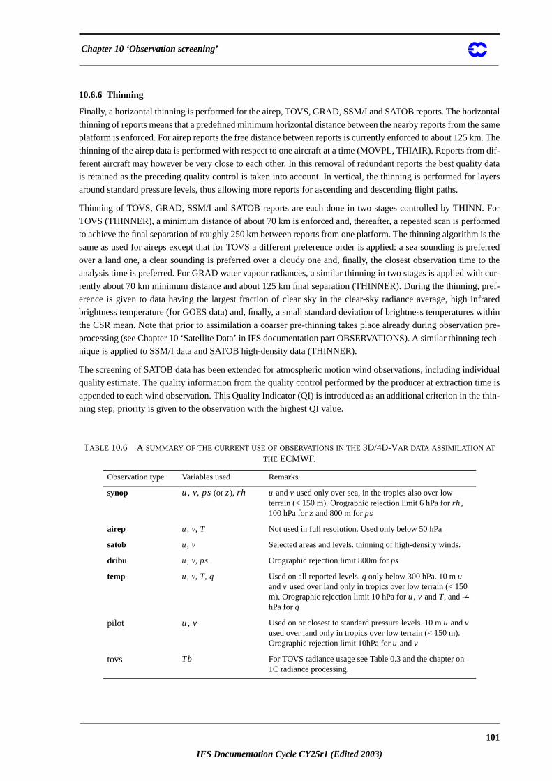
Chapter 10 ‘Observation screening’
ntal
e same
m. The
dif-
ity data
layers
For
ormed
is the
referred
to the
h cur-
pref-
frared
s within
on pre-
tech-
ividual
e is
thin-
10.6.6 Thinning
Finally, a horizontal thinning is performed for the airep, TOVS, GRAD, SSM/I and SATOB reports. The horizo
thinning of reports means that a predefined minimum horizontal distance between the nearby reports from th
platform is enforced. For airep reports the free distance between reports is currently enforced to about 125 k
thinning of the airep data is performed with respect to one aircraft at a time (MOVPL, THIAIR). Reports from
ferent aircraft may however be very close to each other. In this removal of redundant reports the best qual
is retained as the preceding quality control is taken into account. In vertical, the thinning is performed for
around standard pressure levels, thus allowing more reports for ascending and descending flight paths.
Thinning of TOVS, GRAD, SSM/I and SATOB reports are each done in two stages controlled by THINN.
TOVS (THINNER), a minimum distance of about 70 km is enforced and, thereafter, a repeated scan is perf
to achieve the final separation of roughly 250 km between reports from one platform. The thinning algorithm
same as used for aireps except that for TOVS a different preference order is applied: a sea sounding is p
over a land one, a clear sounding is preferred over a cloudy one and, finally, the closest observation time
analysis time is preferred. For GRAD water vapour radiances, a similar thinning in two stages is applied wit
rently about 70 km minimum distance and about 125 km final separation (THINNER). During the thinning,
erence is given to data having the largest fraction of clear sky in the clear-sky radiance average, high in
brightness temperature (for GOES data) and, finally, a small standard deviation of brightness temperature
the CSR mean. Note that prior to assimilation a coarser pre-thinning takes place already during observati
processing (see Chapter 10 ‘Satellite Data’ in IFS documentation part OBSERVATIONS). A similar thinning
nique is applied to SSM/I data and SATOB high-density data (THINNER).
The screening of SATOB data has been extended for atmospheric motion wind observations, including ind
quality estimate. The quality information from the quality control performed by the producer at extraction tim
appended to each wind observation. This Quality Indicator (QI) is introduced as an additional criterion in the
ning step; priority is given to the observation with the highest QI value.
TABLE 10.6 ASUMMARY OF THE CURRENT USE OF OBSERVATIONS IN THE3D/4D-VAR DATA ASSIMILATION AT
THE ECMWF.
Observation type Variables used Remarks
synop u, v, ps (or z), rh u andv used only over sea, in the tropics also over lowterrain (< 150 m). Orographic rejection limit 6 hPa forrh,100 hPa forz and 800 m forps
airep u, v, T Not used in full resolution. Used only below 50 hPa
satob u, v Selected areas and levels. thinning of high-density winds.
dribu u, v, ps Orographic rejection limit 800m forps
temp u, v, T, q Used on all reported levels.q only below 300 hPa. 10 muandv used over land only in tropics over low terrain (< 150m). Orographic rejection limit 10 hPa foru, v andT, and -4hPa forq
pilot u, v Used on or closest to standard pressure levels. 10 mu andvused over land only in tropics over low terrain (< 150 m).Orographic rejection limit 10hPa foru andv
tovs Tb For TOVS radiance usage see Table 0.3 and the chapter on1C radiance processing.
101
IFS Documentation Cycle CY25r1 (Edited 2003)

Part II: ‘Data assimilation’
ometer
perature
it set
nd re-
eport
erage
are then
ere the
ormed
r sea-
ection
related
ssed by
pressed
rate is
eports
obser-
ad bal-
Apart from this thinning, the other observation dependent decisions involved by the screening of the scatter
data come essentially from the application of a sea-ice contamination test from the model sea-surface-tem
analysis, using a minimum threshold of 273 K, and a high-wind rejection test with an upper-wind speed lim
to 25 for the higher of the scatterometer and background winds (FGWIND).
In addition, the quality flag set in OBSPROC is also applied, and an extra quality control is done on the wi
trieval residual, or the so-called ‘normalized distance to the cone’. After being implicitly checked for each r
through the OBSPROC flag (different from 0 if its value is larger than 3), this quantity is tested in global av
over the 6 hours of the analysis cycle for each of the 19 measurement nodes across the swath. All the data
rejected in bulk if an excessive value is found for any node (more than 1.3 times the expected average) wh
number of data taken into account is judged to be significant (i.e. more than 500). While the first check, perf
locally, aims at avoiding geophysical effects not explained by the transfer function CMOD4, such as rain o
state effects in the vicinity of deep lows, this global quality control on the distance to the cone allows the det
of technical anomalies not reported in real time by ESA that are likely to affect the measurements in a cor
way and at larger scales. Such anomalies, which occur typically in the case of orbital manoeuvres, are mi
the preliminary test of the instrumental quality flag in OBSPROC.
10.6.7 A summary of the current use of observations
A summary of the current status of use of observations in the 3D-Var data assimilation is given inTable 10.6.
10.6.8 Compression of the ODB
After the observation screening roughly a fraction of 1/10 of all the observed data are active and so the com
observation array for the minimization run only contains those data (COMPRES ). The large compression
mainly driven by the number of TOVS data, since after the screening there are only 10–20% of the TOVS r
left, whereas for the conventional observations the figure is around 40%. As a part of the compression, the
vations are re-sorted amongst the processors for the minimization job in order to achieve a more optimal lo
grad Tb Water vapour channel of Meteosat-7. Data used only whenclear-sky fraction above 70%, satellite zenith angle below 60deg and model orography below 1500m. Data from somehours around local midnight are excluded (number of hoursvaries with season). Thinned.
paob ps Used south of 19oS. Orographic rejection limit 800 m for ps
scatt u, v Not used in full resolution. Used if SST is warmer than 273K or if both observed and background wind less than 25
ssm/i tcwv Thinned, used over sea.
The variables are as inTable 10.1, with the addition thatTb stands for brightness temperature andtcwvstands for total cloud water vapour. The observation types are shortened bysynop for synoptic surfaceobservations,airep for aircraft reports,satob for satellite cloud track winds,dribu for drifting buoyreports,tempfor radiosonde soundings,pilot for wind soundings,tovsfor satellite temperature soundings,grad for geostationary clear-sky radiance,paob for pseudo observations of surface pressure andscatt forscatterometer reports
TABLE 10.6 ASUMMARY OF THE CURRENT USE OF OBSERVATIONS IN THE3D/4D-VAR DATA ASSIMILATION AT
THE ECMWF.
Observation type Variables used Remarks
m s 1–
m s 1–
102
IFS Documentation Cycle CY25r1 (Edited 2003)
Chapter 10 ‘Observation screening’
as set
f obser-
bserva-
re those
nment
e other
cessors
refore,
ation
erva-
e. For
are in-
edistri-
to the
pendent
ecking
g each
nicated.
cessor
ilation
rs. This
urrently,
cation
dered as
ancing of the parallel computer.
10.7 AMASSIVELY -PARALLEL COMPUTING ENVIRONMENT
The migration of operational codes at the ECMWF to support a massively-parallel computing environment h
a requirement for reproducibility. The observation screening needs to result in exactly the same selection o
vations when different numbers of processors are used for the computations. As mentioned earlier, in the o
tion screening there are the two basic types of decision to be made. Independent decisions, on one hand, a
where no information concerning any other observation or decision is needed. In a parallel-computing enviro
these decisions can be happily made by different processors fully in parallel. For dependent decisions, on th
hand, a global view of the observations is needed which implies that some communication between the pro
is required. The observation array is, however, far too large to be copied for each individual processor. The
the implementation of observation screening at the ECMWF is such that only the minimum necessary inform
concerning the reports is communicated globally.
The global view of the observations is provided in the form of a global ‘time–location’ array for selected obs
tion types. That array contains compact information concerning the reports that are still active at this stag
instance, the observation time, location and station identifier as well as the owner processor of that report
cluded. The time–location array is composed at each processor locally and then collected for merging and r
bution to each processor. After the redistribution, the array is sorted locally within the processors according
unique sequence number. Thus, every processor has exactly the same information to start with, and the de
decisions can be performed in a reproducible manner independently of the computer configuration.
The time–location array is just large enough for all the dependent decisions, except for the redundancy ch
of the multilevel temp and pilot reports. This is a special case, in the sense that the information concernin
and every observed variable from each level is needed. Hence, the whole multilevel report has to be commu
The alternative to this would be to force the observation clusters of the multilevel reports always into one pro
without splitting them. In that case the codes responsible for the creation of the observation arrays for assim
would need to ensure the geographical integrity of the observation arrays distributed amongst the processo
is, however, not possible in all the cases, and the observation screening has to be able to cope with this. C
it is coded in such a way that only a limited number of multilevel temp and pilot reports, based on the time–lo
array, are communicated between the appropriate processors as copies of these common stations.
APPENDIX A
A.1 BAD REPORTING PRACTICE OF SYNOP AND TEMP REPORTS
The way the synoptic surface stations report mass observations (pressure or geopotential height) is consi
bad if the
• station altitude is above 800 m and station reports mean sea level pressure
• station altitude is above 800 m and station reports 1000 hpa level
• station altitude is above 1700 m and station reports 900 hpa level
• station altitude is below 300 m and station reports 900 hpa level
• station altitude is above 2300 m and station reports 850 hpa level
• station altitude is below 800 m and station reports 850 hpa level
• station altitude is above 3700 m and station reports 700 hpa level
103
IFS Documentation Cycle CY25r1 (Edited 2003)

Part II: ‘Data assimilation’
gpm or
level.
ted in
m/s
by
evel
rface
for the
cember
the as-
orth
• station altitude is below 2300 m and station reports 700 hpa level
• station altitude is below 3700 m and station reports 500 hpa level
The reporting practice is also considered as bad if the station reports 500 gpm, 1000 gpm, 2000 gpm, 3000
4000 gpm level pressure, respectively, and station altitude is more than 800 m different from the reported
For temp geopotentials the reporting practice is considered as bad if the
• station altitude is above 800 m and station reports 1000 hpa level
• station altitude is above 2300 m and station reports 850 hpa level
• station altitude is above 3700 m and station reports 700 hpa level
A.2 REVISED BACKGROUND QUALITY CONTROL FOR SELECTED OBSERVATIONS
The background quality-control rejection limits are applied more strictly for some observation types than sta
Table 10.1. The special cases are the following ones
• airep wind observations with zero wind speed are rejected if the background wind exceeds 5
• for airep and dribu wind observations the rejection limit is multiplied by 0.5, and for pilot wind
0.8
• for satob wind observations the rejection limit is multiplied by 0.1, except below 700 hPa l
where it is multiplied by 0.2
• no background quality control is applied for scatt winds
• for dribu surface pressure observations the rejection limit is multiplied by 0.9, and for paob su
pressure by 0.7
• for airep temperature observations the rejection limit is multiplied by 1.6
A.3 USE OF ATMOSPHERIC MOTION WINDS
This appendix describes those parts of the ECMWF assimilation system which involves some special code
AMW case, i.e. the data selection and the FG quality check. It refers to the operational status as from De
1996. A thinning procedure was introduced for high-density winds in Spring 1998.
A.3.1 Data selection
There are several model independent checks which AMW data have to pass in order to be considered for
similation process:
Check on longitude/latitude
• AMW must be within a circle of 55˚ from the sub-satellite point
Check on levels depending on the computational method
• WW CMW and WVMW must be above 400 hPa
• VIS CMW must be below 700 hPa
• IR CMW can be used at all levels.
Check on land/sea
• All AMW over sea are used
• AMW over land is not used north of 20ºN. .
• For Meteosat (0º mission) instead of 20ºN this threshold is 35ºN to allow usage of AMW over n
Africa.
104
IFS Documentation Cycle CY25r1 (Edited 2003)

Chapter 10 ‘Observation screening’
his is
erved
r
pres-
t 500
he
an the
the
• For Meteost (63º mission) the use of AMW has been extended over Asia if above 500 hPa. T
restriced for longitudes east of 30ºE.
• AMW are blacklisted over the Himalayas as a precautionary measure.
• AMW over land south of 20ºN (35ºN for Meteosat) is used if above 500 hPa.
Check on satellite (35ºN for Meteosat) is used if above 500 hPa.
This is a temporary selection on certain channels or satellites. At present channels and satellite used are:
• METEOSAT cloud tracked winds with 90 min temporal sampling
• METEOSAT IR (not at medium level), VIS, WV
• METEOSAT HVIS, also at asynoptic times, only if
(
• GOES IR & WV (NOT at asynoptic times)
• GMS IR & VIS
A.3.2 Background quality check
The background quality check is based on a comparison of the AMW deviation from the background. Obs
wind components are checked together. The AMW is flagged withj = 1 or 2 or 3 if this deviation squared is greate
than a predetermined multiple ERRLIM * ZREJMOD of its estimated variance, as given by the following ex
sion:
if [ D2 > (sfg 2 + sobs 2 ) * ERRLIMj * ZREJMOD] then flag=j where D 2 = 1/2 (Du2 +D v2) with Du, Dv
wind component deviations from background; sfg std of the background wind component error (mean foru and
v); sobs std of the observation wind component error, 2 for levels below 700 hPa included, 3.5 a
hPa, 4.3 at 400 hPa and 5 for all levels above; ERRLIMj is 8 for j=1, 18 for j=2 and 20 for j=3. T
value of ZREJMOD depends on the level of AMW and normally its value is:
• ZREJMOD = 0.2 for low level
• ZREJMOD = 0.1 for all others levels
A special check or asymmetric check is applied when the observed speed is more than 4 slower th
background speed SPDfg. This check has a more restrictive rejection limit:
• ZREJMOD = 0.15 at low level
• ZREJMOD = 0.07 in the tropics
• ZREJMOD = 0.075 – 0.00125 * SPDfg all others
• ZREJMOD = 0.0 if SPDfg > 60 (observation gets always flagj = 3)
When the data is passed to the following variational quality control its probability of being used depend on
flag j. With flag j = 1 the data will be assimilated, with flagj =2 it will be given an intermediate probability and
might be used or not and finally the analysis will reject all data withj = 3
QI2 0≡Automatic Quality Control PASSED≡
m s 1– m s 1–
m s 1– m s 1–
m s 1–
m s 1–
105
IFS Documentation Cycle CY25r1 (Edited 2003)

Part II: ‘Data assimilation’
106
IFS Documentation Cycle CY25r1 (Edited 2003)

IFS Documentation Cycle CY25r1
e that is
the sea-
od. The
field.
6-hour
lysis is
mod-
Part II: D ATA ASSIMILATION
CHAPTER 11 Analysis of snowSnow depth is a model prognostic variable that needs to be analysed. Its analysis is performed in a modul
currently separated from the analysis of the atmosphere and of the soil wetness. This module includes also
surface temperature, sea-ice fraction and screen-level temperature and relative humidity.
Table of contents
11.1 Organization
11.2 Snow-depth analysis
11.3 Technical aspects
11.1 ORGANIZATION
The snow analysis is a 3-D sequential analysis performed every 6 hours using a successive correction meth
snow-depth background (units: m) is estimated from the short-range forecast of snow water equivalent
(units: m of water equivalent) and snow density (units : kg m-3):
Thesnow-depth analysis is performed using snow-depth observations and the snow-depth background
If snow-depth observations are not available, the snow accumulation/melting is simulated from the model
forecast and a weak relaxation towards climatology is added. Thesnow climateis used to ensure the stability of
the scheme and to give a seasonal snow trend in areas without any snow observations.
11.2 SNOW-DEPTH ANALYSIS
The observations are snow depths from SYNOP reports. The background is defined above. The ana
done using a Cressman spatial interpolation:
The weight function is the product of functions of the horizontal distance and vertical displacement (
el minus obs height) between the observation and analysis points:
,
Sb Wsb
ρsb
Sb 1000 Wsb×
ρsb
--------------------------=
Sa
So Sb
Sa Sb
wnSno
n 1=
N
∑
wnn 1=
N
∑---------------------------+=
wn r h
w H r( )ν h( )=
107
IFS Documentationn Cycle CY25r1 (Edited 2003)
Part II: ‘Data assimilation’
d below.
r each
.
now
is
le of
s:
pth cli-
hive
et to an
where
and
The snow depth is preserved when the model height is above the observing station, but it is severely reduce
The influence distances are set to km and m.
In addition to the preliminary quality control in the observation data base, the following checks are applied fo
grid point :
• if only snow depth observations below 140 cm are accepted.
• this limit is reduced to 70 cm if .
• snow-depth observations are rejected if they differ by more than 50 cm from the background
• when only one snow-depth observation is available within the influence radius , the s
depth increments are set to zero.
• snow-depth analysis is limited to 140 cm.
• snow-depth increments are set to zero when larger than mm (where
expressed in Celsius)
• snow-depth analysis is set to zero if below 0.04 cm
• if there is no snow in the background and in more than half of the observations within a circ
radius , the snow-depth increment is kept to zero.
The analysis of snow depth is finally weighted with climatological values to provide the final analysi
The relaxation coefficient is set to 0.02 corresponding to a time scale of 12.5 days. The global snow de
matology is taken fromFosterand Davy (1988). Finally the snow density from the background is used to arc
the analysis in terms of snow water equivalent :
The snow density is unchanged in the analysis process :
Areas with permanent snow and ice (defined using the Global Land Cover Characterization product) are s
arbitrary high value at each analysis cycle ( ).
H r( ) maxrmax
2 r2–
rmax2 r2+
--------------------- 0,
=
ν h( ) 1= if 0 h<
ν h( )hmax
2 h2–
hmax2 h2+
-----------------------= if hmax h 0< <–
ν h( ) 0= if h hmax–<
rmax 250= hmax 300=
T2mb 8°C<
T2mb 8°C>
rmax
160 16T2mb–( ) T2m
b
rmax
Sclim
Sa 1 a–( )Sa aSclim+=
a
Wsa ρs
b Sa×1000
------------------=
ρsa ρs
b=
Wsa 10m=
108
IFS Documentation Cycle CY25r1 (Edited 2003)

Chapter 11 ‘Analysis of snow’
vel anal-
alysis,
ing snow
tine
MA-
d ze-
d
th-
ial.
tions
con-
s.
cern
, slowly
s-
erti-
11.3 TECHNICAL ASPECTS
The snow analysis software is implemented as a branch of the more comprehensive surface and screen-le
ysis (SSA) package. The other branches currently include two-metre temperature and relative humidity an
and also sea surface temperature and sea-ice fraction analyses. The program organization when perform
analysis is roughly as follows:
• SSA
• CONTROL_SSA
• INISNW
• SCAN_DDR
• COORDINATES
• GETFIELDS
• SCAN_CMA
• SCAN_OBS
• LAND_OBS
• INITIAL_REJECTION
• REDUNDANT_OBS
• SNOW_ANALYSIS
• SUCSNW
• SCAN_OBS
• FG2OBS
• SUCSNW
• SNOW_FG
• FDB_OUTPUT
• PRINT_SUMMARY
• PLOTDATA
• FEEDBACK
The main programSSAcallsCONTROL_SSAwhere most of the setup and namelist handling are done. Rou
INISNW performs initialization of the actual snow analysis by sensing the size of the observation array file (C
file) in SCAN_DDRand generating latitudinal coordinates that stem from the model resolution in concern an
ros of the Bessel function.
After this, all input fields are read into memory inGETFIELDS. They consist of the snow water equivalent an
snow density from the first-guess (6-hour forecast), 2 m temperature first guess, snow-depth climate (varies mon
ly with a linear temporal interpolation), land/sea mask and finally the orography in a form of the geopotent
In SCAN_CMAobservations are read into memory and a quick validity check of the non-applicable observa
for this analysis is performed. Furthermore, the land/sea mask is calculated inLAND_OBS for the retained snow
depth observation points.
Additional screening is done inINITIAL_REJECTION and inREDUNDANT_OBS. The former one sets up an
internal table where all the observations which survived from the quick screening are placed with a minimum
text information. This routine rejects some of the observations entered into the table due to inconsistencie
The routineREDUNDANT_OBSremoves time duplicates and retains the observations of the station in con
with the closest (and the most recent) to the analysis time. Since only synoptic observations are considered
moving platform handling present in theREDUNDANT_OBS is not applicable to the snow analysis.
The actual snow analysis is performed underSNOW_ANALYSIS. The analysis technique is Cressman’s succe
sive correction method (routineSUCSNW). The structure functions are set to be separable in horizontal and v
109
IFS Documentation Cycle CY25r1 (Edited 2003)

Part II: ‘Data assimilation’
t is in
ivalent
arture at
ducing
d.
r
(in
s a
d in
se of
cal directions. A special mountain region handling is performed, depending whether the datum or grid poin
the valley or at high altitudes, as explained before.
The snow-depth background (i.e. first guess) field is constructed from the model first-guess snow water equ
and snow density. Once the snow-depth first guess field is present, it is used to calculate the first guess dep
snow-depth observation points. This increment is finally added to the snow depth fields at grid points pro
the final snow depth output field, which is output in routineFDB_OUTPUT.
The accuracy of the analysis is estimated inPRINT_SUMMARYwhere some important statistics are summarize
The internal observation table can be printed if requested fromPLOTDATA and an updated observation file fo
feedback purposes can be created in routineFEEDBACK.
The main logicals of the namelist NAMSSA are :
• L_SNOW_ANALYSIS : When set to TRUE, the snow analysis is performed.
• L_SNOW_DEPTH_ANA : When set to TRUE, the snow analysis is performed in snow depth
opposition to snow water equivalent assuming a constant value of 250 kg m-2 for observed snow
density).
• L_USE_SNOW_CLIMATE : When set to TRUE, a relaxation of the snow analysis toward
monthly climatology is performed with a time scale of 12.5 days (this constant is hard code
SNOW_FG).
• L_USE_FG_FIELD : When set to TRUE the snow analysis is set to the first-guess value (no u
observations) and there is no relaxation to climatology.
110
IFS Documentation Cycle CY25r1 (Edited 2003)
IFS Documentation Cycle CY25r1
quence,
urs and
temper-
idity at
Firstly,
ements
s a two-
inter-
ments
e first-
n and
pairs
ve the
(hard
CHAPTER 12 Land-surface analysis
12.1 INTRODUCTION
Soil temperature and soil water content are prognostic variables of the forecasting system and, as a conse
they need to be initialised at each analysis cycle. Currently the land surface analysis is performed every 6 ho
is decoupled from the atmospheric analysis. The absence of routine observations on soil moisture and soil
ature requires to use proxy data. The ECMWF soil analysis relies on SYNOP temperature and relative hum
screen-level (2 m) available on the GTS (around 12000 reports over the globe are provided every 6 hours).
a screen-level analysis is performed for temperature and humidity. Secondly, the screen-level analysis incr
are used as inputs to perform the analysis in the soil.
12.2 SCREEN-LEVEL ANALYSIS
12.2.1 Methodology
Two independent analyses are performed for 2 m temperature and 2 m relative humidity. The method used i
dimensional univariate statistical interpolation. In a first step, the background field (6 h or 12 h forecast) is
polated horizontally to the observation locations using a bilinear interpolation scheme and background incre
are estimated at each observation location .
The analysis increments at each model grid-point are then expressed as a linear combination of th
guess increments (up to values) :
(12.1)
where are optimum weights given (in matrix form) by :
(12.2)
The column vector (dimension ) represents the background error covariance between the observatio
the model grid-point . The matrix describes the error covariances of background fields between
of observations. The horizontal correlation coefficients (structure functions) of and are assumed to ha
following form:
(12.3)
where is the horizontal separation between points and and the e-folding distance taken to 300 km
coded in subroutine OIINC).
Therefore :
(12.4)
∆ Xi i
X ja∆ j
N
X ja∆ Wi Xi∆×
i 1=
N
∑=
Wi
B O+( )W b=
b N ij N N× B
b B
µ i j,( ) 12---
rij
d-----
2
– exp=
rij i j d
B i j,( ) σb2 µ i j,( )×=
111
IFS Documentationn Cycle CY25r1 (Edited 2003)
‘’
vation
idered
cean
is the
ecent) to
ted if it
% of the
dew-
s
the
with the standard deviation of background errors.
The covariance matrix of observation errors is set to where is the standard deviation of obser
errors and the identity matrix.
The standard deviations of background and observation errors are set respectively to 1.5 K and 2 K for temperature
and 5% and 10% for relative humidity. The number of observations closest to a given grid point that are cons
to solve(12.1)is (scanned within a radius of 1000 km). The analysis is performed over land and o
but only land (ocean) observations are used for model land (ocean) grid points.
12.2.2 Quality controls
Gross quality checks are first applied to the observations such as and where
dewpoint temperature. Redundant observations are also removed by keeping only the closest (and more r
the analysis time.
Observation points that differ by more than 300 m from the model orography are rejected.
For each datum a check is applied based on statistical interpolation methodology. An observation is rejec
satisfies :
(12.5)
where has been set to 3, both for temperature and humidity analyses.
The number of used observations every 6 hours varies between 4000 and 6000 corresponding to around 40
available observations.
The final relative humidity analysis is bounded between 2% and 100%. The final MARS archived product is
point temperature that uses the 2 m temperature analysis to perform the conversion :
(12.6)
with
(12.7)
12.2.3 Technical aspects
The technical aspects are similar to the snow analysis (seeChapter 11) expect for the computation of the analysi
increments obtained from the subroutineOIUPD instead ofSUCSNW (Cressman interpolation).
SubroutineOISET selects the closest observations from a given grid-point.
SubroutineOIINC provides the analysis increments from Equations(12.1) and (12.2), by first computing
(in subroutineEQUSOLVE- inversion of a linear system) which does not depend upon
position of the analysis gridpoint and then estimating (in subroutineDOT_PRODUCT).
Most of the control parameters of the screen-level analysis are defined in the namelist NAMSSA:
1) C_SSA_TYPE : ‘t2m’ for temperature analysis and ‘rh2m’ for relative humidity analysis
2) L_OI : ‘ true’ for statistical interpolation and ‘false’ for Cressman interpolation
σb
O σo2 I× σo
I
N 50=
RH 2 100,[ ]∈ T Td> Td
Xi∆ γ σo2 σb
2+>
γ
Ta
Td 17.502 273.16 32.19 Ψ×–×17.05 Ψ–
---------------------------------------------------------------------=
Ψ RHa( )log 17.502Ta 273.16–
Ta 32.19–----------------------------×+=
N
q B O+( ) 1– X∆=
bTq
112
IFS Documentation Cycle CY25r1 (Edited 2003)

Chapter 12 ‘Land-surface analysis’
ments
ce of
n the
single-
omly.
educe
ligible
3) N_OISET : number of observations (parameter )
4) SIGMAB : standard deviation of background error (parameter )
5) SIGMAO : standard deviation of observation error (parameter )
6) TOL_RH : Tolerance criteria for RH observations (parameter in Equation(12.5))
7) TOL_T : Tolerance criteria for T observations (parameter in Equation(12.5))
8) SCAN_RAD_2M(1) : Scanning radius for available observations (set to 1000 km)
12.3 SOIL ANALYSIS
The soil analysis scheme is based on an “local” optimum interpolation technique as described inMahfouf(1991)
andDouvilleet al. (2001). The analysis increments from the screen-level analysis are used to produce incre
for the water content in the first three soil layers (correponding to the root zone) :
(12.8)
and for the first soil temperature layer :
(12.9)
The coefficients and are defined as the product of optimum coefficients and minimising the varian
analysis error and of empirical functions , and reducing the size of the optimum coefficients whe
coupling between the soil and the lower boundary layer is weak.
(12.10)
and
(12.11)
with
(12.12)
where represents the correlation of background errors between parameters and .
The statistics of background errors have been obtained from a series of Monte-Carlo experiments with a
column version of the atmospheric model where initial conditions for soil moisture have been perturbed rand
They were obtained for a clear-sky situation with strong solar insolation. Empirical functions are aimed to r
soil increments when atmospheric forecast errors contain less information about soil moisture. To obtain neg
Nσb
σo
γγ
θ∆ a Ta Tb–( )× b 100es Ta
d( ) es Tbd( )–
es Ta( )--------------------------------------×+=
T∆ c Ta Tb–( )×=
a b α βF1 F2 F3
ασθ
φσbT
---------- 1σa
RH
σbRH
----------- 2
+ ρTθ ρRHTρRHθ–
=
βσθ
φσbRH
-------------- 1σa
RH
σbRH
----------- 2
+ ρRHθ ρRHTρTθ–
=
φ 1σa
T
σbT
------ 2
+ 1σa
RH
σbRH
----------- 2
+ ρRHT2–=
ρxy x y
113
IFS Documentation Cycle CY25r1 (Edited 2003)
‘’
enith
y situ-
e solar
fficients
ed in
ground
and
soil-moisture corrections during the night and in winter, is a function of the cosine of the mean solar z
angle , averaged over the 6 h prior to the analysis time :
(12.13)
The optimum coefficients are also reduced when the radiative forcing at the surface is weak (cloudy or rain
tations). For this purpose, the atmospheric transmittance is computed from the mean downward surfac
radiation forecasted during the previous 6 hours as :
(12.14)
where is the solar constant.
The empirical function is expressed as :
(12.15)
with and .
The empirical function reduces soil moisture increments over mountainous areas :
(12.16)
where is the model orography, =500 m and =3000 m.
Furthermore, soil moisture increments are set to zero if one of the following conditions is fufilled:
1) The last 6 h precipitation exceeds 0.6 mm
2) The instantaneous wind speed exceeds 10 m s-1
3) The air temperature is below freezing
4) There is snow on the ground
To reduce soil moisture increments over bare soil surfaces, the standard deviations and the correlations coe
are also weighted by the vegetation fraction , where low and high vegetation cover are defin
Chapter 7 of the Physics Documentation.
The statistics of forecast errors necessary to compute the optimum coefficients are given inTable 12.1.
The correlations have been produced from the Monte-Carlo experiments. The standard deviation of back
error for soil moisture is set to 0.01 m3m-3 on the basis of ECMWF forecasts differences between day 1
day 2 of the net surface water budget (precipitation minus evaporation minus runoff).
The standard deviation of analysis error is given by the screen-level analysis from :
F1
µM
F112--- 1 λ µM 0.5–( )[ ]tanh+{ }= λ 7=
τr
Rg⟨ ⟩
τr
Rg⟨ ⟩SoµM--------------
µM
=
So
F2
F2
0 τr τrmin<
τr τrmin–
τrmax τrmin–------------------------------ τrmin τr τrmax< <
1 τr τrmax>
=
τrmin 0.2= τrmax 0.9=
F3
F3
0 Z Zmax>
Z Zmax–
Zmin Zmax–-----------------------------
2
Zmin Z Zmax< <
1 Z Zmin<
=
Z Zmin Zmax
Cv cL cH+=
σθ
σa
114
IFS Documentation Cycle CY25r1 (Edited 2003)
Chapter 12 ‘Land-surface analysis’
d ca-
rature
ect soil
sum
(12.17)
From the values chosen for the screen-level analyis and %.
Soil moisture increments are such that they keep soil moisture within the wilting point and the fiel
pacity values, i.e. :
• if then
• if then
Finally the coefficients providing the analysis increments are :
(12.18)
and
(12.19)
The coefficient is such that soil temperature is more effective during night and in winter, when the tempe
errors are less likely to be related to soil moisture. This way, 2 m temperature errors are not used to corr
moisture and soil temperature at the same time.
In the 12 h 4D-Var configuration, the soil analysis is performed twice during the assimilation window and the
of the increments is added to the background values at analysis time.
TABLE 12.1 STATISTICS OF BACKGROUND ERRORS FOR SOIL MOISTURE DERIVED FROMMONTE-CARLO
EXPERIMENTS
Coefficient Value
–0.82
–0.92
–0.90
0.83
0.93
0.91
1.25 K
9.5 %
–0.99
1
σa2
----- 1
σb2
----- 1
σo2
-----+=
σaT 1.2K= σa
RH 4.47=
θ∆ θpwp
θcap
θb θcap< θa min θcap θb θ∆+,( )=
θb θpwp> θa max θpwp θb θ∆+,( )=
a Cv α F1×× F2F3=
b Cv β F1×× F2F3=
c 1 F2–( )F3=
c
ρTθ1
ρTθ2
ρTθ3
ρRHθ1
ρRHθ2
ρRHθ3
σbT
σbRH
ρRHT
115
IFS Documentation Cycle CY25r1 (Edited 2003)

‘’
116
IFS Documentation Cycle CY25r1 (Edited 2003)

IFS Documentation Cycle CY25r1
117
IFS Documentationn Cycle CY25r1 (Edited 2003)
Part II: D ATA ASSIMILATION
CHAPTER 13 Sea surface temperature and sea-iceanalysisTHIS CHAPTER IS NOT YET AVAILABLE

Part II: ‘Data assimilation’
118
IFS Documentation Cycle CY25r1 (Edited 2003)
IFS Documentation Cycle CY25r1
” Ka-
ed as
ix; and
a sub-
to the
he ma-
odi-
The
of the
r the
SK-
in the
ifferent
roes as
ow, and
Part II: D ATA ASSIMILATION
CHAPTER 14 Reduced-rank Kalman filter
Table of contents
14.1 The modified change-of-variable
14.2 The Hessian singular vector calculation
14.1 THE MODIFIED CHANGE -OF-VARIABLE
From the point of view of the analysis, the reduced-rank Kalman filter (sometimes known as the “simplified
lman filter) consists of a modification to the change-of-variable. The control variable for the analysis is defin
(14.1)
where is the static change of variable used in 3D- and 4DVar; is a small, square, upper-triangular matr
is an orthogonal matrix which rotates the control variable so that the leading few elements correspond to
space of interest, such as the space spanned by a set of singular vectors.
The background cost function corresponding to the change of variable defined byEq. (14.1) is
(14.2)
where .
The aim of the reduced-rank Kalman filter is to choose the matrices and to be good approximations
corresponding sub-matrices from the true covariance matrix of background error (in the space defined by t
trices and ). The algorithm is described in detail by Fisher (1998) [ECMWF rd Tech Memo 260]. The m
fied change-of-variable is completely specified by two sets of vectors and for .
vectors define the subspace of interest, while for each , the vector defines the action of the inverse
true covariance matrix of background error on .
The main namelist or the reduced rank Kalman filter is NAMSKF. This contains LSKF, the global switch fo
modified change of variable; NSKFVECS, the number of pairs of vectors and ; and CINSKFY and CIN
FZ, which are the names of the files containing the vectors and respectively. The remaining variables
namelist are used in the Hessian simplified vector calculation, and are described later.
The setup routine for the reduced-rank Kalman filter isSUSKF. After reading the namelist NAMSKF to find how
many vectors to read, and from which files,SUSKFreads the vectors into SKFROT (inyomskf) and into
ZZVECS. Both sets of vectors are read using the routineREADVEC, which expects spectral fields of vorticity,
divergence, specific humidity, temperature and LNSP. The fields must be on model levels, but may be of a d
spectral truncation to that of the analysis increments, in which case they are truncated or padded with ze
appropriate. The vectors are usually produced by the Hessian singular vector calculation described bel
χ XT U 0F I
XL δx=
L UX
Jb δxTL TXT E FT
F IXL δx=
E UTU FTF+=
E F
L Xsk zk k 1…NSKFVECS=
sk k zk
sk
sk zk
sk zk
sk zk
zk
119
IFS Documentationn Cycle CY25r1 (Edited 2003)
Part II: ‘Data assimilation’
eturned
pace
alized
ach of
U. The
re sym-
er.
ation
owing
ariable
tter
riance
d us-
trix
pts are
. The
ack-
flow-
memo
essian
de-
s. The
must be scaled by the reciprocal of the eigenvalue which is stored in the GRIB header for each field, and is r
in the optional argument ofREADVEC. The vectors are transformed to control vector space and then to a s
with a Euclidean inner product by calls toCHAVAR, CHAVARINAD andLCZTOIFS.
Next, the orthogonal transformation represented by the matrix inEq. (14.1)is constructed. This transformation
consists of a sequence of Householder matrices (i.e. matrices of the form , where is a norm
vector). The transformation is constructed so that it sets to zero all but the first NSKFVECS elements of e
the vectors in SKFROT. The vectors which define the transformation are stored in SKFROT (inyomskf), overwtrit-
ing the previous content. The non-zero elements of the transformed vectors are retained in the array Z
transpose of the orthogonal transform is applied to the vectors in ZZVEC. Since the Householder matrices a
metric, the transpose of is equivalent to applying the sequence of Householder matrices in reverse ord
At this stage, SKFROT contains the matrix and ZU contains the matrix in the following equation (equ
11 of Fisher, 1998)
(14.3)
The matrix is upper-triangular, so the elements of and may be determined by back-substitution. Foll
this calculation, may not be exactly symmetric, due to rounding errors and the fact that the change-of-v
is not exactly invertible. It is explicitly symmetrized by replacing each element by .
The matrix inEq. (14.1)is the Cholesky square root of . The decomposition requires that the la
matrix is positive definite. This is also the condition for positive definiteness of the background error cova
matrix implied by the change of variable. The Cholesky decomposition of the matrix is performe
ing the NAG routineF07FDF. If the decomposition fails due to an indefinite matrix, then the elements of the ma
are reduced by a factor of 2 and the Cholesky decomposition is attempted again. A maximum of 4 attem
made.
The elements of the matrix are stored in the leading NSKFVECS elements of each vector of SKFMAT
remaining elements contain the matrix .
The modified change-of-variable is applied inCVAR2, CVAR2IN, CVAR2AD, andCVAR2INAD. In the case of
CVAR2, the code corresponds exactly to the change of variable defined inEq. (14.1). The inverse, adjoint and in-
verse-adjoint of the change ofCVAR2 are similar. The inverse makes use of the following equation, and uses b
substitution to apply the matrix .
. (14.4)
14.2 THE HESSIAN SINGULAR VECTOR CALCULATION
The reduced-rank Kalman filter requires as input pairs of vectors which satisfy , where is a
dependent approximation to the true covariance matrix of background error. Fisher (1998) [ECMWF rd tech
260] describes how pairs of vectors satisfying this requirement may be calculated during the course of a “H
singular vector” calculation. That is, a singular vector calculation in which the inner product at initial time is
fined by the Hessian matrix of an analysis cost function. The vectors are partially-evolved singular vector
vectors are produced during the adjoint model integration.
XI 2uuT–( ) u
Xsk
X
X S
Z E FT
F G
S0
=
S E FE
Eij Eij E ji+( ) 2⁄
U E FTF–( )
E FTF–( )
F
UF
U 1–
U 0F I
1–U 1– 0
FU 1– I=
zk Pf( )1–sk= Pf
sk
zk
120
IFS Documentation Cycle CY25r1 (Edited 2003)
Chapter 14 ‘Reduced-rank Kalman filter’
cal-
8,
ed. For
wise,
a using
by
ctors
part of
STOP
1 and
set to
scalar
sed for
matrix
ed. A
alcu-
s
ed by
ll to
e Hes-
vec-
radient
ect
The Hessian singular vector calculation is controlled using the namelist NAMLCZ. The global switch for the
culation is LJACDAV. Initial and final time inner products are selected by NLANTYPE. For NLANTYPE=6 or
the initial time inner product is defined by the analysis Hessian. Otherwise, the spectral inner product is us
NLANTYPE=8 or 9, the final time inner product is defined by the background error covariance matrix. Other
the energy inner product is used. The final time inner product may be restricted to a given geographic are
the variables ALAT1, ALON1, ALAT and ALON3. The optimization time is specified in units of timesteps
NJDSTOP. The maximum number of iterations to be performed byJACDAV (see below) is specifed by NITERL.
The calculation will stop when this number of iterations has been performed, or when NEIGEVO singular ve
have been calculated.
The control-level routine isCUN3, which is called directly fromCNT0. Much of the first part ofCUN3 is con-
cerned with initialization of observations, etc. which are needed by the analysis Hessian calculation. This
the code is essentially the same as the corresponding part ofCVA1, and will not be described here.
The Hessian singular vector calculation is unusual in that it explicitly changes the values of NCONF and N
during the calculation. During the parts of the calculation which resemble an analysis, NCONF is set to 13
NSTOP is set to zero. When the calculation resembles the ordinary singular vector calculation, NCONF is
601 and NSTOP is set to the optimization time for the singular vector calculation defined by NJDSTOP. The
product is also recalculated at various times in the code. In general, however, a spectral inner product is u
most of the calculation. When other inner products are required, they are calculated using an explicit weight
rather than by resetting the SCALP array.
After the initializations for the Hessian calculation, the trajectory for the singular vector calculation is creat
starting vector for the singular vector calculation is initialized, and the gradient for zero control variable is c
lated and saved in VAZG (inyomcva).
The singular vectors are calculated by a call toNALAN2, which writes them to the file svifs.CUN3reads the vec-
tors and callsCNT3TL to give the singular vectors at final time. These are written to the file svevo. The vector
required for the reduced rank Kalman filter are written during the tangent linear integration at a step specifi
NWRISKF (in NAMSKF). The vectors required by the reduced rank Kalman filter are produced by a ca
CNT3AD. The switch LWRISKF (also in NAMSKF) determines whether the vectors and are written.
NALAN2 provides an interface to the main generalized eigenvector solver,JACDAV. The main task ofNALAN2
is to write the singular vectors to the file svifs, and to perform some diagnostics.JACDAV calculates the Hessian
singular vectors as the solutions to the following generalized eigenvector equation
(14.5)
where denotes the tangent linear model, defines the inner product at optimization time, and is th
sian of an analysis cost function. The algorithm requires operators which apply and to arbitrary
tors. These operations are represented in the code by the subroutinesOPKandOPMrespectively. SubroutineOPM
calculates a Hessian-vector product as a finite difference between the gradient for the input vector, and the g
for zero control vector which is in VAZG. The gradient for the input vector is calculated by a call toSIM4D.
JACDAV starts with an initial matrix of KSTART vectors. The columns of are orthonormalized with resp
to the initial time inner product by a call toMORTHODM. That is, they are made to satisfy .MOR-
THODM also appliesOPK andOPM to the vectors.
Next, the following small ordinary eigenvalue problem is solved
sk
zk
sk zk
M TWMx λJ″x=
M W J ″M TWM J ″
V VVTJ″V I=
121
IFS Documentation Cycle CY25r1 (Edited 2003)
Part II: ‘Data assimilation’
onal
duced
izing
red re-
ited
)
It can be
algo-
(14.6)
The eigenvalues of this problem are the Ritz values (i.e. approximations to the eigenvalues) ofEq. (14.5). The re-
sidual, , for the leading unconverged Ritz value is selected. The residual is orthog
to the columns of in the Euclidean sense. A vector which is orthogonal with respect to the Hessian is pro
by first calculating an approximate solution to the linear equation , and then explicitly orthonormal
by a call toMORTHODM. The linear equation is solved by a call toPCGBFGS, which implements a precondi-
tioned conjugate gradient algorithm. The accuracy of the solution is determined by GREDBFGS (the requi
duction in the norm of the error), and NINNER (the maximum number of iterations to be performed). A lim
memory BFGS preconditioner is used, which is applied by the routineBFGS. The memory size (in pairs of vectors
is given by MEMBFGS.
Once the vector has been determined, it is included as a new column of , and the process is repeated.
shown that if the linear equation is solved exactly, then the algorithm is equivalent to a Lanczos
rithm. If it is solved approximately, the algorithm resembles the Jacobi-Davidson method.
VTMTWMVy θy=
r M TWMVy θJ″Vy–=
VJ″v r=
v
v VJ″v r=
122
IFS Documentation Cycle CY25r1 (Edited 2003)

IFS Documentation Cycle CY25r1
.
fard,
, A.,
al
as-
at C-
var-
ag
.
c
,
r, F.
or-
Part II: D ATA ASSIMILATION
REFERENCES
Alduchov, O. A. and Eskridge, R.E., 1996: Improved Magnus form approximation of saturation vapor pressureJ.
Appl. Met., 35, 601–609.
Andersson, E., Pailleux, J., Thépaut, J.–N., Eyre, J. R., McNally, A. P., Kelly, G. A. and Courtier, P., 1994: Use
of cloud–cleared radiances in three/four–dimensional variational data assimilation. Q. J. R. Meteorol. Soc., 120,627–653
Andersson, E., Haseler, J., Undén, P., Courtier, P., Kelly, G., Vasiljevic, D., Brankovic, C., Cardinali, C., Gaf
C., Hollingsworth, A., Jakob, C., Janssen, P., Klinker, E., Lanzinger, A., Miller, M., Rabier, F., Simmons
Strauss, B., Thépaut, J.–N. and Viterbo, P., 1998:The ECMWF implementation of three dimensional variation
assimilation (3D–Var). Part III: Experimental results. To appear inQ. J. R. Meteorol. Soc.
Andersson, E., 1997: Implementation of variational quality control. Proc. ECMWF workshop on “Non–linear
pects of data assimilation”, Reading, 9–11 September 1996.
Andersson, E. and Järvinen, H., 1999: Variational quality control.Q. J. R. Meteorol. Soc., 125, 697–722
Attema, E., P. W., 1986:An experimental campaign for the determination of the radar signature of the ocean
band.Proc. Third International Colloquium on Spectral Signatures of Objects in Remote Sensing, Les Arcs,
France, ESA,SP-247, 791-799.
Bartello, P. and Mitchell, H. L., 1992: A continuous three–dimensional model of short–range forecast error co
iance.Tellus, 44A, 217–235.
Blondin, C., 1991: ‘Parametrization of land surface processes in numerical weather prediction’. Pp. 31–54 inLand
surface evaporation: measurement and parametrization, T. J. Schmugge and J.–C. André, Eds., Springer–Verl
Bouttier, F., Derber, J. and Fisher, M., 1997: The 1997 revision of the Jb term in 3D/4D–Var. ECMWF Tech
Memo. 238.
Buck, A.L., 1981: New equations for computing vapor pressure and enhancement factor.J. Appl. Met., 20, 1527–
1532.
Buizza, R., 1994: Sensitivity of optimal unstable structures.Q. J. R. Meteorol. Soc., 120, 429–451
Cardinali, C., Andersson, E., Viterbo, P., Thépaut, J.–N. and Vasiljevic, D., 1994: Use of conventional surface ob-
servations in three–dimensional variational data assimilation. ECMWF Tech. Memo. 205.
Chelton, D., B., Freilich, M. H., and S. K, Esbensen. 2000:Satellite observations of the wind jets off the Pacifi
coast of Central America. Part I: Case studies and statistical characteristics.Mon. Wea. Rev., 128, 1,993-2,018.
Courtier, P., Thépaut, J.–N. and Hollingsworth, A., 1994: A strategy for operational implementation of 4D–Var
using an incremental approach.Q. J. R. Meteorol. Soc., 120, 1367–1388
Courtier, P., Andersson, E., Heckley, W., Pailleux, J., Vasiljevic, D., Hamrud, M., Hollingsworth, A., Rabie
and Fisher, M., 1998: The ECMWF implementation of three dimensional variational assimilation (3D–Var). I: F
mulation.Q. J. R. Meteorol. Soc., 124, 1783-1807.
Douville, H., Viterbo, P., Mahfouf, J.-F. and Beljaars, A. C. M. (2001): “Evaluation of the optimum interpolation
and nudging techniques for soil moisture analysis using FIFE data”Mon. Wea. Rev., 128, 1733-1756
123
IFS Documentationn Cycle CY25r1 (Edited 2003)
Part II: ‘Data assimilation’
.
Dept.
onal
a-
, NC
r
D-
ht of
el.
lgo-
o. ?.
r
ined
nary
an
re-
Var
-
Eyre, J. R., 1989: Inversion of cloudy satellite sounding radiances by nonlinear optimal estimation.Q. J. R. Mete-
orol. Soc., 115, 1001–1037.
Eyre, J. R., 1991: A fast radiative transfer model for satellite sounding systems. ECMWF Tech. Memo. 176
Eyre, J.R. 1992: A bias correction scheme for simulated TOVS brightness temperatures. ECMWF Research
Tech. Memo. 186.
Eyre, J. R., Kelly, G. A., McNally, A. P., Andersson, E. and Persson, A.,1993: Assimilation of TOVS radiance in-
formation through one–dimensional variational analysis.Q. J. R. Meteorol. Soc., 119, 1427–1463.
Fisher, M. and Courtier, P., 1995: Estimating the covariance matrices of analysis and forecast error in variati
data assimilation, ECMWF Tech. Memo. 220.
Freilich, M. S. and Anderson, D., 1997: Ambiguity removal and assimilation of scatterometer data.Q. J. R. Mete-
orol. Soc., 123, 491–518
Foster , D.J. and R.D. Davy, 1988: Global snow depth climatology. U.S. Air Force Environmental Tech. Applic
tions Center/TN-88/006, 48 pp. [Available from National Climate Data Center, 151 Patton Avenue, Asheville
28801]
Gaffard, C., Roquet, H., Hansen, B., Andersson, E. and Anderson, D., 1997: Impact of the ERS–1 scatteromete
wind data on the ECMWF 3D–Var assimilation system. To appear inQ. J. R. Meteorol. Soc.
Gauthier, P. and Thepaut, J.-N., 2000: Impact of the digital filter as a weak constraint in the pre-operational 4
Var assimilation system of Meteo-France. Submitted to Mon. Weather Rev.
Geleyn, J.–F., 1988: Interpolation of wind, temperature and humidity values from the model levels to the heig
meaurement.Tellus, 40, 347–351
Gerard, E, and R. Saunders, 1999: 4D-Var assimilation of SSM/I total column water vapour in the ECMWF mod
ECMWF RD Tech Memo no.270.
Gilbert, J. C. and Lemaréchal, C., 1989:Some numerical experiments with variable storage quasi-Newton a
rithms.Math. Prog., B25, 407–435
Harris, B. 1997: A revised bias correction scheme for TOVS radiances. ECMWF Technical Memorandum N
Hersbach, H., Isaksen, L, Leidner, S. M. and P. A. E. M. Janssen 2003:The impact of SeaWinds scatteromete
data in the ECMWF 4D-Var assimilation system. In preparation.
Hollingsworth, A. and Lönnberg, P., 1986: The statistical structure of short–range forecast errors as determ
from radiosonde data. Part I: The wind field.Tellus, 38A, 111–136
Ingleby, N. B. and Lorenc, A. C., 1993: Bayesian quality control using multivariate normal distributions.Q. J. R.
Meteorol. Soc.,119, 1195–1225.
Isaksen, L, (1997). Impact of ERS scatterometer data in the ECMWF 4D-Var assimilation system. Prelimi
studies. InSpace at the Service of our Environment, 1,829-1,851, Florence, Italy, May 1997, ESTEC, Europe
Space Agency [SP-414]. Available from ESA Publications Division, ESTEC Noordwijk, The Netherlands.
Isaksen, L. and A. C. M. Stoffelen, 2000: ERS scatterometer wind data impact on ECMWF’s tropical cyclone fo
casts.IEEE Trans. Geosci. Remote Sens., 38 (4), 1,885-1,892.
Järvinen, H. and Undén, P., 1997: Observation screening and first guess quality control in the ECMWF 3D-
data assimilation system. ECMWF Tech. Memo. 236.
Järvinen, H, S Saarinen and P Undén, 1996:User’s guide for blacklisting. 51pp. Available on request from EC
124
IFS Documentation Cycle CY25r1 (Edited 2003)
IFS Documentation Cycle CY25r1
va-
WF
F.
G2
al
al
-
d the
ined
F
.
l 1.
ing.
.
mber,
0
or-
MWF, Shinfield Park, RG2 9AX, Reading, Berkshire, England.
Järvinen, H., E. Andersson and F. Bouttier, 1999:Variational assimilation of time sequences of surface obser
tions with serially correlated errors. submitted to Tellus, 28pp. also, RD Tech Memo no.266.
Kelly, G. and Pailleux, J., 1988:Use of satellite vertical sounder data in the ECMWF analysis system. ECM
Tech. Memo. 143.
Kelly, G., Andersson, E., Hollingsworth, A., Lönnberg, P., Pailleux, J. and Zhang, Z., 1991: Quality control of op-
erational physical retrievals of satellite sounding data.Mon. Weather Rev., 119, 1866–1880.
Köpken, C., 2002:Monitoring and assimilation of Meteosat radiances within the 4DVAR system at ECMW
EUMETSAT/ECMWF Fellowship Report No. 9. Available from ECMWF, Shinfield Park, Reading Berkshire R
9AX, UK.
Leidner, S. M., Hofman, R. N. and Augenbaum, J., 1999: SeaWinds Satterometer Real-Time BUFR Geophysic
Data Product User’s Guide Version 1.0, available from ECMWF and AER
Leidner, S. M., R.N. Hoffman and J. Augenbaum, 2000: SeaWinds Scatterometer Real-Time BUFR Geophysic
Data Product, User’s Guide Version 2.3.0, NOAA/NESDIS.
Leidner, S. M, Isaksen, L, and R. N. Hoffman, 2003:Impact of NSCAT winds on tropical cyclones in the EC
MWF 4D-Var assimilation system,Mon. Wea. Rev., 131, In press.
Lönnberg, P, 1989: Developments in the ECMWF analysis system. ECMWF Seminar on Data assimilation an
use of satellite data. 5-9 September 1988, 75-119.
Lönnberg, P. and Hollingsworth, A., 1986: The statistical structure of short-range forecast errors as determ
from radiosonde data. Part II: The covariance of height and wind errors.Tellus, 38A, 137–161.
Lönnberg, P and D Shaw, 1985:Data selection and quality control in the ECMWF analysis system. ECMW
Workshop on The Use And Quality Control of Meteorological Observations, 6-9 November 1984, 225-254
Lönnberg, P and D Shaw (Eds.), 1987: ECMWF Data Assimilation Scientific Documentation. Research Manua
Lorenc, A. C., 1986: Analysis methods for numerical weather prediction.Q. J. R. Meteorol. Soc., 112, 1177–1194.
Lorenc, A. C., 1988: Optimal nonlinear objective analysis.Q. J. R. Meteorol. Soc., 114, 205–240.
Lott ,F. and Miller M.J., 1997: A new subgrid-scale orographic drag parametrization : its formulation and test
Q.J.R. Meteorol. Soc., 123, 101-127.
Louis, J.–F., 1979: A parametric model of vertical eddy fluxes in the atmosphere.Boundary-Layer Meteorol., 17.
187–202.
Louis, J.–F., Tiedtke, M. and Geleyn, J.–F., 1982: ‘A short history of the PBL parametrization at ECMWF’. Pp
59–80 in Proc. ECMWF Workshop on Planetary boundary layer parameterization, Reading, 25–27 Nove
1981
Lynch, P., 1993: Digital Filters for Numerical Weather Prediction. HIRLAM Technical Report No 10.
Lynch, P., 1996: The Dolph-Chebyshev Window: A Simple Optimal Filter. Mon. Weather Rev., 125, 655–66
Machenhauer, B., 1977: On the dynamics of gravity oscillations in a shallow water model, with application to n
mal mode initialization.Contrib. Atmos. Phys.,50, 253-271.
McNally, A. P. and Vesperini, M., 1996: Variational analysis of humidity information from TOVS radiances. Q. J.
R. Meteorol. Soc., 122, 1521–1544.
125
IFS Documentationn Cycle CY25r1 (Edited 2003)

Part II: ‘Data assimilation’
ta
infield
n
RG2
Pp.
anog-
al-
the
dy
.
998
o ap-
Ham-
. , Un-
an
-
96.
ce
at-
ical
Mahfouf, J.-F., 1991: Analysis of soil moisture from near surface parameters : a feasibility study.J. Appl. Meteor.,
30, 1534-1547
Mahfouf, J.-F., Buizza, R., and Errico, R. M., 1997: Strategy for including physical processes in the ECMWF da
assimilation system. In Proceedings of the ECMWF Workshop on non-linear aspects of data assimilation, Sh
Park, Reading, RG2 9AX, 9–11 September 1996
Mahfouf, J.-F., 1998: Influence of physical processes on the tangent-linear approximation
Matricardi, M., Chevallier, F. and Tjemkes, S., 2001: An improved fast radiative transfer model for the assimilatio
of radiance observations. Tech. Memo. No 345, Available from ECMWF, Shinfield Park, Reading, Berkshire
9AX, UK
Pailleux, J.,1990: ‘A global variational assimilation scheme and its application for using TOVS radiances’.
325–328 in Proc. WMO International Symposium on Assimilation of observations in meteorology and oce
raphy”, Clermont–Ferrand, France
Parrish, D. F. and Derber, J. C., 1992: The National Meteorological Center’s spectral statistical interpolation an
ysis system.Mon. Weather Rev., 120, 1747–1763.
Phalippou, L., 1996: Variational retrieval of humidity profile, wind speed and cloud liquid–water path with
SSM/I: Potential for numerical weather prediction.Q. J. R. Meteorol. Soc., 122, 327–355.
Phalippou, L. and Gérard, É., 1996: ‘Use of precise microwave imagery in numerical weather forecasting’. Stu
report to the European Space Agency. Available from ECMWF.
Portabella, M., and A. Stoffelen, 2000:Quality control and wind retrieval for SeaWinds.Scientific report WR-
2002-01, Koninklijk Nederlands Meteorologisch Instituut, The Netherlands.
Rabier, F. and McNally, A., 1993: Evaluation of forecast error covariance matrix. ECMWF Tech. Memo. 195
Rabier, F., McNally, A., Andersson, E., Courtier, P., Undén, P., Eyre, J., Hollingsworth, A. and Bouttier, F., 1:
The ECMWF implementation of three dimensional variational assimilation (3D–Var). II: Structure funtions. T
pear inQ. J. R. Meteorol. Soc.
Rabier, F., Mahfouf, J.-F., Fisher, M., Järvinen, H. , Simmons. A., Andersson, E., Bouttier, F., Courtier, P.,
rud, M., Haseler, J., Hollingsworth, A., Isaksen, L., Klinker, E., Saarinen, S., Temperton, C., Thépaut, J.–N
dén, P., and Vasiljevic, D., 1997a: Recent experimentation on 4D-Var and first results from a simplified Kalm
filter. ECMWF Tech. Memo. 240.
Rabier, F., Thépaut, J.–N. and Courtier, P., 1997b: Four-dimensional variational assimilation at ECMWF. In Pro
ceedings of the ECMWF Seminar on data assimilation, Shinfield Park, Reading, RG2 9AX, September 19
Saunders, R. W. and Matricardi, M., 1998: ‘A fast forward model for ATOVS (RTATOV)’. Tech. Proc. 9th Inter-
national TOVS Study Conf., Igls, Austria, 20–26 February, 1997. 11 pp.
Savijärvi, H., 1995: Error growth in a large numerical forecast system.Mon. Wea. Rev., 123, 212–221.
Simmons, A. J. and Burridge, D., 1981:An energy and angular momentum conserving vertical finite differen
scheme and hybrid coordinate.Mon. Weather Rev., 109, 758–766.
Simmons, A. J. and Chen, J., 1991: The calculation of geopotential and the pressure gradient in the ECMWF
mospheric model: Influence on the simulation of the polar atmosphere and on temperature analyses.Q. J. R. Me-
teorol. Soc., 117, 29–58.
Sherlock, V. J., 1999: ISEM-6: Infrared Surface Emissivity Model for RRTOV-6. Forecasting Research Techn
126
IFS Documentation Cycle CY25r1 (Edited 2003)
IFS Documentation Cycle CY25r1
-
on
-
pects.
or-
Report No 299, Available from Met Office, London Road, Bracknell, Berkshire RG12 2SZ, UK
Stoffelen, A. 1999:Scatterometry. PhD Thesis, available from KNMI
Stoffelen, A. and Anderson, D., 1997: Ambiguity removal and assimilation of scatterometer data.Q. J. R. Meteorol.
Soc., 123, 491–518.
Temperton, C., 1988: Implicit normal mode initialization.Mon. Weather Rev., 116, 1013-1031.
Temperton, C., 1989: Implicit normal mode initialization for spectral models.Mon. Weather Rev., 117, 436-451.
Thépaut, J.–N., Courtier, P., Belaud, G., and Lemaitre, G., 1996: Dynamical structure functions in a four-dimen
sional variational assimilation: a case study. Q. J. R. Meteorol. Soc., 122, 535–561.
Tiedtke, M., 1989: A comprehensive massflux scheme for cumulus parametrization in large-scale models.Mon.
Weather Rev., 117, 1779–1800.
Tomassini, M., LeMeur, D. and Saunders, R., 1997: Satellite wind observations of hurricanes and their impact
NWP model analyses and forecasts. To appear inMon. Weather Rev.
Vasiljevic, D., Cardinali, C. and Undén, P., 1992: ‘ECMWF 3D–Variational assimilation of conventional obser
vations’. In Proc. ECMWF workshop on Variational assimilation with emphasis on three–dimensional as
Reading, 9–12 November 1992.
Wergen, W., 1987: Diabatic nonlinear normal mode initialisation for a spectral model with a hybrid vertical co
dinate. ECMWF Tech. Report 59.
127
IFS Documentationn Cycle CY25r1 (Edited 2003)