IEEE TRANSACTIONS ON PATTERN ANALYSIS AND …sczhu/papers/prints/C4_PAMI.pdf · C4: Exploring...

C4: Exploring Multiple Solutionsin Graphical Models by Cluster Sampling

Jake Porway, Student Member, IEEE, and Song-Chun Zhu, Fellow, IEEE

Abstract—This paper presents a novel Markov Chain Monte Carlo (MCMC) inference algorithm called C4—Clustering with

Cooperative and Competitive Constraints—for computing multiple solutions from posterior probabilities defined on graphical models,

including Markov random fields (MRF), conditional random fields (CRF), and hierarchical models. The graphs may have both positive

and negative edges for cooperative and competitive constraints. C4 is a probabilistic clustering algorithm in the spirit of Swendsen-

Wang [34]. By turning the positive edges on/off probabilistically, C4 partitions the graph into a number of connected components (ccps)

and each ccp is a coupled subsolution with nodes connected by positive edges. Then, by turning the negative edges on/off

probabilistically, C4 obtains composite ccps (called cccps) with competing ccps connected by negative edges. At each step, C4 flips the

labels of all nodes in a cccp so that nodes in each ccp keep the same label while different ccps are assigned different labels to observe

both positive and negative constraints. Thus, the algorithm can jump between multiple competing solutions (or modes of the posterior

probability) in a single or a few steps. It computes multiple distinct solutions to preserve the intrinsic ambiguities and avoids premature

commitments to a single solution that may not be valid given later context. C4 achieves a mixing rate faster than existing MCMC

methods, such as various Gibbs samplers [15], [26] and Swendsen-Wang cuts [2], [34]. It is also more “dynamic” than common

optimization methods such as ICM [3], LBP [21], [37], and graph cuts [4], [20]. We demonstrate the C4 algorithm in line drawing

interpretation, scene labeling, and object recognition.

Index Terms—Markov random fields, computer vision, graph labeling, probabilistic algorithms, constraint satisfaction, Monte Carlo.

Ç

1 INTRODUCTION

1.1 Motivations and Objective

MANY vision tasks, such as scene labeling [22], [31], [32],object detection/recognition [11], [36], segmentation

[8], [35], and graph matching [6], [24], are formulated asenergy minimization (or maximum a posteriori probability)problems defined on graphical models—Markov randomfields [3], [15], conditional random fields (CRFs) [22], [23],or hierarchical graphs [14], [40]. These optimizationproblems become exceedingly difficult when there aremultiple solutions, i.e., distinct modes with high probabil-ities and, in some cases, equal probability.

Fig. 1 shows examples of typical scenarios that havemultiple, equally likely solutions in the absence of furthercontext. The top row shows the well-known Necker Cube,which has two valid 3D interpretations. The middle row isthe Wittgenstein illusion in which the drawing can appearto be either a duck or a rabbit. Without further context, wecannot determine the correct labeling. The bottom rowshows an aerial image for scene labeling. It can be explainedas either a roof with vents or a parking lot containing cars.

Computing multiple solutions is important for preservingthe intrinsic ambiguities and avoiding early commitment to asingle solution which, even if it is currently the globally

optimal one, may turn out to be less favorable when latercontext arrives. However, it is a persistent challenge to enablealgorithms to climb out of local optima and to jump betweensolutions far apart in the state space. Popular energyminimization algorithms, such as Iterative ConditionalModes (ICM) [3], Loopy Belief Propagation (LBP) [21], [37],and graph cuts [4], [20], compute one solution and thus do notaddress this problem. Existing MCMC algorithms, such asvarious Gibbs samplers [15], [26], Data-Driven Markov ChainMonte Carlo (DDMCMC) [35], and Swendsen-Wang (SW)cuts [2], [34], promise global optimization and ergodicity inthe state space, but often need long waiting time in movingbetween distinct modes, which needs a sequence of luckymoves up the energy landscape before it goes down.

In this paper, our objective is to develop an algorithmthat can discover multiple solutions by jumping out ofequal probability states and thus preserve the ambiguitieson rather general settings:

1. The graph can be flat, such as an MRF or CRF, orhierarchical, such as a parse graph.

2. The graph may have positive (cooperative) andnegative (competitive or conflicting) edges for bothhard or soft constraints.

3. The probability (energy) defined on the graph isquite general, even with energy terms involvingmore than two nodes.

In vision, it is safe to assume that the graph is locallyconnected and we do not consider the worst-case scenariowhere graphs are fully connected.

1.2 Related Work in the Literature

In the 1970s, many problems, including line drawinginterpretation and scene labeling, were posed as constraint

IEEE TRANSACTIONS ON PATTERN ANALYSIS AND MACHINE INTELLIGENCE, VOL. 33, NO. 9, SEPTEMBER 2011 1713

. J. Porway is with the R&D Division of The New York Times.

. S.-C. Zhu is with the Departments of Statistics and Computer Science,University of California, Los Angeles (UCLA), and the Lotus Hill ResearchInstitute.

Manuscript received 10 May 2010; revised 4 Dec. 2010; accepted 11 Dec.2010; published online 9 Feb. 2011.Recommended for acceptance by K. Murphy.For information on obtaining reprints of this article, please send e-mail to:[email protected], and reference IEEECS Log NumberTPAMI-2010-05-0362.Digital Object Identifier no. 10.1109/TPAMI.2011.27.

0162-8828/11/$26.00 � 2011 IEEE Published by the IEEE Computer Society

satisfaction problems (CSPs). The CSPs were either solvedby heuristic search methods [30] or constraint propagationmethods [1], [28]. The former keeps a list of open nodes forplausible alternatives and can backtrack to explore multiplesolutions. However, the open list can become too long tomaintain when the graph is large. The latter iterativelyupdates the labels of nodes based on their neighbors. Onewell-known constraint propagation algorithm is the relaxa-tion labeling method by Rosenfeld et al. [32].

In the 1980s, the famous Gibbs sampler—a probabilisticversion of relaxation labeling—was presented by Gemanand Geman [15]. The update of labels is justified in a solidMCMC and MRF framework and thus is guaranteed tosample from the posterior probabilities. In special cases, theGibbs sampler is equal to belief propagation [30] forpolytrees and to dynamic programming in chains. TheGibbs sampler is found to slow down critically when anumber of nodes in the graph are strongly coupled.

Fig. 2 illustrates an example of the difficulty withstrongly coupled graphs using the Necker Cube. The sixinternal lines of the figure are divided into two couplinggroups: (1-2-3) and (4-5-6). Lines in each group must havethe same label (concave or convex) to be valid, as theyshare the two “Y”-junctions. Thus, updating the label of asingle line in a coupled group does not move at all unlesswe update the label of the whole group together, i.e., allsix labels in one step.

The problem is that we don’t know which nodes in thegraph are coupled and to what extent they are coupled forgeneral problems with large graphs. In 1987, a break-through came from two physicists, Swendsen and Wang[34], who proposed a cluster sampling technique. The SWmethod finds coupled groups, called “clusters,” dynami-cally by turning the edges in the graph on/off according tothe probabilities defined on these edges. The edge prob-ability measures the coupling strengths. Unfortunately,their algorithm only works for the Ising and Potts models.We will discuss the SW method in later sections.

There were numerous attempts made to improve MCMCmethods in the 1990s (see Liu [25] for surveys), such as theblock Gibbs sampler [26]. Green formulated reversible jumpsin 1995 [17] following the jump-diffusion algorithm byGrenander and Miller [18]. In 1999, Cooper and Friezeanalyzed the convergence speed of SW using a path couplingtechnique and showed that the SW method has a polynomialmixing time when the nodes in the graph are connected to aconstant number of neighbors [7]. Nevertheless, it was alsoshown that SW could mix slowly under conditions whengraphs were heavily or fully connected [16].

In the 2000s, a few non-MCMC methods generatedremarkable impacts on the vision community, for example,the LBP algorithm by Weiss [37] and the graph cutalgorithms by Boykov et al. and Kolmogorov and Rother[4], [20]. These algorithms are very fast and work well on aspecial class of graph structures and energy functions. Inaddition, techniques such as survey propagation [5] havehad great success in statistical physics. In the case ofmultimodal energy functions, however, it can be difficultfor these techniques to converge properly, as we will see.

On the MCMC side, Tu and Zhu developed theDDMCMC algorithm for image segmentation in 2002 [35],which uses bottom-up discriminative probabilities to drivethe Markov chain moves. They also developed a“K-adventurer” procedure to keep multiple solutions. TheDDMCMC method was also used by Dellaert [29] fortracking bee dances. Dellaert also used MCMC to explorecorrespondences for structure-from-motion problems, evenincorporating a “jump parameter” to allow the algorithm tojump to new solutions [9]. In 2005, Barbu and Zhu proposedthe SW-cut algorithm [2] which, for the first time, general-ized the SW method to arbitrary probabilities models. Aswe will discuss in later sections, the SW-cut did notconsider negative edges, high-order constraints, or hier-archical graphs and is less effective in swapping betweencompeting solutions. The C4 algorithm in this paper is adirect generalization of the SW-cut algorithm [2].

1.3 Overview of the Major Concepts of C4

In this paper, we present a probabilistic clusteringalgorithm called Clustering Cooperative and CompetitiveConstraints (C4) for computing multiple solutions ingraphical models. We consider two types of graphs:

Adjacency graphs treat each node as an entity, such as apixel, a superpixel, a line, or an object, which has to be

1714 IEEE TRANSACTIONS ON PATTERN ANALYSIS AND MACHINE INTELLIGENCE, VOL. 33, NO. 9, SEPTEMBER 2011

Fig. 2. Swapping between the two interpretations of the Necker cube.Locally coupled labels are swapped with alternate labelings to enforceglobal consistency. See text for explanation.

Fig. 1. Problems with multiple solutions: (top) the Necker cube, (middle)the Wittgenstein illusion, and (bottom) an aerial image interpreted aseither a roof with vents or a parking lot with cars. Ambiguities should bepreserved until further context arrives.

labeled in K-classes (or colors). Most MRFs and CRFs usedin computer vision are adjacency graphs.

Candidacy graphs treat each node as a candidate orhypothesis, such as a potential label for an entity, or adetected object instance in a window, which has to beconfirmed (“on”) or rejected (“off”). In other words, thegraph is labeled with K ¼ 2 colors.

As we will show in Section 2.1, an adjacency graph canalways be converted to a bigger candidacy graph. In bothcases, the tasks are posed as graph coloring problems onMRF, CRF, or hierarchical graphs. There are two types ofedges expressing either hard or soft constraints (orcoupling) between the nodes.

Positive edges are cooperative constraints that favor the twonodes having the same label in an adjacency graph or beingturned on (or off) simultaneously in a candidacy graph.

Negative edges are competitive or conflicting constraintsthat require the two nodes to have different labels in anadjacency graph or one node to be turned on and the otherturned off in a candidacy graph.

In Fig. 2, we show that the Necker cube can be representedin an adjacency graph, with each line being a node. The sixinternal lines are linked by six positive edges (in green) andtwo negative edges (in red and wiggly). Lines 2 and 4 have anegative edge between them as they intersect with eachother, as do lines 3 and 6. We omit the labeling of the six outerlines for clarity.

In this paper, the edges play computational roles and areused to dynamically group nodes which are stronglycoupled. On each positive or negative edge, we define anedge probability (using bottom-up discriminative models) forthe coupling strength. Then, we design a protocol for turningthese edges on and off independently according to their edgeprobabilities, respectively, for each iteration. The protocol iscommon for all problems, while the edge probabilities areproblem specific. This probabilistic procedure turns off someedges, and all of the edges that remain “on” partition thegraph into some connected components (ccps).

A ccp is a set of nodes that are connected by the positiveedges. For example, Fig. 2 has two ccps: ccp1 includes nodes1-2-3 and ccp2 includes nodes 4-5-6. Each ccp is a locallycoupled subsolution.

A cccp is a composite connected component that consistsof a number of ccps connected by negative edges. Forexample, Fig. 2 has one cccp containing ccp1 and ccp2. Eachcccp contains some conflicting subsolutions.

At each iteration, C4 selects a cccp and updates the labelsof all nodes in the cccp simultaneously so that 1) nodes ineach ccp keep the same label to satisfy the positive orcoupling constraints, and 2) different ccps in the cccp areassigned different labels to observe the negative constraints.

Since C4 can update a large number of nodes in a singlestep, it can move out of local modes and jump effectivelybetween multiple solutions. The protocol design groups thecccps dynamically and guarantees that each step follows theMCMC requirements, such as detailed balance equations,and thus it samples from the posterior probability.

We evaluate C4 against other popular algorithms in theliterature by two criteria.

1. The speed at which they converge to solutions. Insome studied cases, we know the global minimumsolutions.

2. The number of unique solution states generated bythe algorithms over time. This measures how“dynamic” an algorithm is.

3. The estimated marginal probability at each site in thegraphical model after convergence.

The remainder of the paper is organized as follows: InSection 2, we describe the graph representation and anoverall protocol for C4. In Section 3, we introduce theC4 algorithm on flat graphs and show the sampling of Pottsmodels with positive and negative edges as a special case.In Section 4, we show experiments on generalized C4

outperforming BP, graph cuts, SW, and ICM for somesegmentation, labeling, and CRF inference tasks. We extendC4 to hierarchical graphs in Section 5 and show experimentsfor hierarchical C4. Finally, we conclude the paper with adiscussion of our findings in Section 6.

2 GRAPHS, COUPLING, AND CLUSTERING

2.1 Adjacency and Candidacy Graphs

We start with a flat graph G that we will extend to ahierarchical graph in Section 5:

G ¼ <V ; E>; E ¼ Eþ [E�: ð1Þ

Here, V ¼ fvi; i ¼ 1; 2; . . . ; ng is a set of vertices or nodes onwhich variables X ¼ ðx1; . . . ; xnÞ are defined, and E ¼feij ¼ ðvi; vjÞg is a set of edges which is divided into Eþ

and E� for positive (cooperative) and negative (competitiveor conflicting) constraints, respectively. We consider twotypes of graphs for G:

An adjacency graph, where each node vi 2 V is an entity,such as a pixel or superpixel in image labeling, a line in aline drawing interpretation, or an object in scene under-standing. Its variable xi 2 f1; 2; 3; . . . ; Kig is a label or color.MRFs and CRFs in the literature belong to this category,and the task is to color the nodes V in K colors.

A candidacy graph, where each node vi 2 V is acandidate or hypothesis, such as a potential label assign-ment for an entity, an object instance detected by bottom-upmethods, or a potential match of a point to another point ingraph matching. Its variable xi 2 f0on0; 0off 0g is a Booleanwhich confirms (“on”) or rejects (“off”) the candidate. Inother words, the graph is labeled with K ¼ 2 colors. In thegraph matching literature [6], the candidacy graph isrepresented by a assignment matrix.

An adjacency graph can always be transferred to a biggercandidacy graph by converting each node vi into Ki nodesfxijg. xij 2 f0on0; 0off 0g represents xi ¼ j in the adjacencygraph. These nodes observe a mutual exclusion constraintto prevent fuzzy assignments to xi.

Fig. 3 shows this conversion. The adjacency graph Gadj ¼<Vadj; Eadj> has six nodes Vadj ¼ fA;B;C;D;E; Fg and eachhas 3 � 5 potential labels. The variables are Xadj ¼ðxA; . . . ; xF Þ with xA 2 f1; 2; 3; 4; 5g and so on. We convertit to a candidacy graph Gcan ¼ <Vcan; Ecan> with 24 nodesVcan ¼ fA1; . . . ; A5; . . . ; F1; . . . ; F4g. Node A1 represents acandidate hypothesis that assigns xA ¼ 1. The Xcan ¼ðxA1

; . . . ; xF4Þ are Boolean variables.

Represented by the graph G, the vision task is posed asan optimization problem that computes a most probable

PORWAY AND ZHU: C4: EXPLORING MULTIPLE SOLUTIONS IN GRAPHICAL MODELS BY CLUSTER SAMPLING 1715

interpretation with a posterior probability pðXj IÞ or anenergy function EðXÞ:

X� ¼ arg max pðXj IÞ ¼ arg min EðXÞ: ð2Þ

To preserve the ambiguity and uncertainty, we maycompute multiple distinct solutions fXig with weightsf!ig to represent the posterior probability:

ðXi; !iÞ � pðXj IÞ; i ¼ 1; 2; . . . ; K: ð3Þ

2.2 Positive and Negative Edges

In conventional vision formulation, edges in the graphs area representational concept and the energy terms in E aredefined on the edges to express the interactions betweennodes. In contrast, Swendsen and Wang [34] and Edwardand Sokal [10] added a new computational role to the edgesin their cluster sampling method. The edges are turned“on” and “off” probabilistically to dynamically form groups(or clusters) of nodes which are strongly coupled. We willintroduce the clustering procedure shortly after the exam-ple below. In this paper, we adopt this notion and the edgesin graph G are characterized in three aspects:

Positive versus negative. A positive edge represents acooperative constraint for two nodes having the same labelin an adjacency graph or being turned on (or off)simultaneously in a candidacy graph. A negative edgerequires the two nodes to have different labels in anadjacency graph or requires one node to be turned on andthe other turned off in a candidacy graph.

Hard versus soft. Some edges represent hard constraintswhich must be satisfied, for example, in line drawinginterpretation or scene labeling, while other edge con-straints are soft and can be expressed with a probability.

Position-dependent versus value-dependent. Edges in adja-cency graphs are generally position-dependent. For example,in an Ising model, an edge between two adjacent nodesposes a soft constraint that they should have the same label(ferromagnetism) or opposite labels (antiferromagnetism).In contrast, edges in candidacy graphs are value-dependentand thus have more expressive power. This is common forvision tasks, such as scene labeling, line drawing inter-pretation, and graph matching. As Fig. 3 illustrates, theedges between nodes in the candidacy graph could beeither positive or negative depending on the valuesassigned to nodes A;B in the adjacency graph.

As we will show in a later section, the positive andnegative edges are crucial for generating connected compo-nents and resolving the problem of node coupling.

2.3 The Necker Cube Example

Fig. 4 shows the construction of a candidacy graph G forinterpreting the Necker cube. For clarity of discussion, weassume the exterior lines are labeled and the task is toassign two labels (concave and convex) to the six inner linessuch that all local and global constraints are satisfied.Therefore, we have a total of 12 candidate assignments ornodes in G.

Based on the theory of line drawing interpretation [27],[33], the two “Y”-junctions pose positive constraints so thatlines 1-2-3 have the same label and lines 4-5-6 have the samelabel. We have 12 positive edges (green) in G to expressthese constraints. The intersection of lines 2 and 4 posesnegative constraints that lines 2 and 4 have opposite labelswhich are shown in the red and wiggly edges in Fig. 4. Thesame is true for lines 3 and 6. The two different assignmentsfor each line should also be linked by a negative edge. Thesenegative edges are not shown for clarity.

In this candidacy graph, the two solutions that satisfy allconstraints are represented by the 2-colors in Fig. 4. The firsthas all nodes 1, 2, and 3 labeled convex (“x”) and all nodes4, 5, and 6 labeled concave (“o”). This solution is currentlyin the “on” state. This would create a valid 3D interpreta-tion where the cube is “coming out” of the page. Thealternative solution has the opposite labeling and creates a3D interpretation of the cube “going in” to the page.

To switch from one solution to the other, we must swapthe junction labels. Each set of nodes, 1-2-3 and 4-5-6,constitutes a corner of the Necker Cube and all have positiveconstraints between them. This indicates that we shouldupdate all of these values simultaneously. We create twoconnected component ccp1 and ccp2 comprised of the couplednodes 1-2-3 and nodes 4-5-6, respectively. If we were to


Fig. 3. Converting an adjacency graph to a candidacy graph. Thecandidacy graph has positive (straight green lines) and negative(wiggled red lines) edges, depending on the values assigned to thenodes in the adjacency graph.

Fig. 4. The Necker cube example. The adjacency graph with 6 nodes(bottom) is converted to a candidacy graph of 12 nodes (top) forconcave and convex label assignments, respectively. Twelve positiveand two negative edges are placed between these candidate assign-ments to ensure consistency.

simply invert the labels of ccp1 or ccp2 alone, we wouldcreate an inconsistent interpretation where all edges in thewhole graph would now have the same label. What we needto do is simultaneously swap ccp1 and ccp2.

Note that we have negative edges between nodes 2 and 4and between nodes 3 and 6. Negative edges can be thoughtof as indicators of multiple competing solutions, as theynecessarily dictate that groups on either end of the edge caneither be (“on,” “off”) or (“off,” “on”), creating two possibleoutcomes. This negative edge connects nodes in ccp1 andccp2, thus indicating that those nodes in the two ccps musthave different labels. We construct a composite connectedcomponent (called cccp), cccp12, encompassing nodes 1-6,we now have a full component that contains all relevantconstraints. Moving from solution 1 to 2 is now as simple asflipping all the nodes simultaneously or, equivalently,satisfying all of the constraints.

In the next section, we explain how we form the ccps andcccps in a formal way.

2.4 Edge Probability for Clustering

On each positive or negative edge, we define an edgeprobability (using bottom-up discriminative models) for thecoupling strength. That is, at each edge e 2 E, we define anauxiliary probability ue 2 f0; 1g or f0on0; 0off 0g, whichfollows an independent probability qe.

In Swendsen and Wang [34], the definition of qe isdecided by the energy term in the Potts model qe ¼ e�2� as aconstant for all e. Barbu and Zhu [2], for the first time,separate qe from the energy function and define it as abottom-up probability: qe ¼ pðlðxiÞ ¼ lðxjÞjF ðxiÞ, F ðxjÞÞ ¼pðe ¼ onjF ðxiÞ; F ðxjÞÞ with F ðxiÞ and F ðxjÞ being localfeatures extracted at nodes xi and xj. This can be learnedthrough discriminative training, for example, by logisticregression and boosting,

pðlðxiÞ ¼ lðxjÞjF ðxiÞ; F ðxjÞÞpðlðxiÞ 6¼ lðxjÞjF ðxiÞ; F ðxjÞÞ

¼Xn

�nhnðF ðxiÞ; F ðxjÞÞ:

On a positive edge e ¼ ði; jÞ 2 Eþ, ue ¼ 0on0 follows aBernoulli probability

ue � Bernðqe � 1ðxi ¼ xjÞÞ:

1ðÞ is Boolean function. It equals 1 if the condition issatisfied and 0 otherwise. Therefore, at the present state X,if the two nodes have the same color, i.e., xi ¼ xj, then theedge e is turned on with probability qe. If xi 6¼ xj, then ue �Bernð0Þ and e is turned off with probability 1. So, if twonodes are strongly coupled, qe should have a higher valueto ensure that they have a higher probability of staying thesame color.

Similarly, for negative edges e 2 E�, ue ¼ 0on0 alsofollows a Bernoulli probability

ue � Bernðqe1ðxi 6¼ xjÞÞ:

At the present state X, if the two nodes have the same colorxi ¼ xj, then the edge e is turned off with probability 1,otherwise e is turned on with probability qe to enforce thatxi and xj stay in different colors.

After sampling ue for all e 2 E independently, we denotethe sets of positive and negative edges that remain “on” as

Eþon � Eþ and E�on � E�, respectively. Then, we have formaldefinitions of the ccp and cccp.

Definition 1. A ccp is a set of vertices fvi; i ¼ 1; 2; . . . ; kg forwhich every vertex is reachable from every other vertex by thepositive edges in Eþon.

Definition 2. A cccp is a set of ccps fccpi; i ¼ 1; 2; . . . ;mg forwhich every ccp is reachable from every other ccp by thenegative edges in E�on.

No two ccps are reachable by positive edges or else theywould be a single ccp. Thus, a cccp is a set of isolated ccpsthat are connected by negative edges. An isolated ccp is alsotreated as a cccp.

In Section 5, we will treat the invalid cases where a ccpcontains negative edges by converting it to a cccp.

To observe the detailed balance equations in MCMCdesign, we need to calculate the probabilities for selecting accp or cccpwhich are determined by the edge probabilities qe.For this purpose, we define their cuts. In general, a cut is theset of all edges connecting nodes between two nodes sets.

Definition 3. Under a current state X, a cut for a ccp is the setall positive edges between nodes in ccp and its surroundingnodes which have the same label:

CutðccpjXÞ ¼ fe : e 2 Eþ; xi ¼ xj; i 2 ccp; j 62 ccpg:

These are the edges that must be turned off probabilistically(with probability 1� qe) in order to form the ccp and the cutdepends on the state X.

Definition 4. A cut for a cccp at a state X is the set of allnegative (or positive) edges connecting the nodes in the cccpand its neighboring node which has different (or same) labels:

CutðcccpjXÞ ¼ fe : e 2 E�; i 2 cccp; j 62 cccp; xi 6¼ xjg[ fe : e 2 Eþ; i 2 cccp; j 62 cccp; xi ¼ xjg:

All of these edges must be turned off probabilistically withprobability 1� qe in order to form the composite connectedcomponent cccp at state X.

As edges in Eþon only connect nodes with the same label,so all nodes in a ccp have the same label. In contrast, alledges in E�on only connect nodes with different labels,adjacent ccps in a cccp must have different labels.

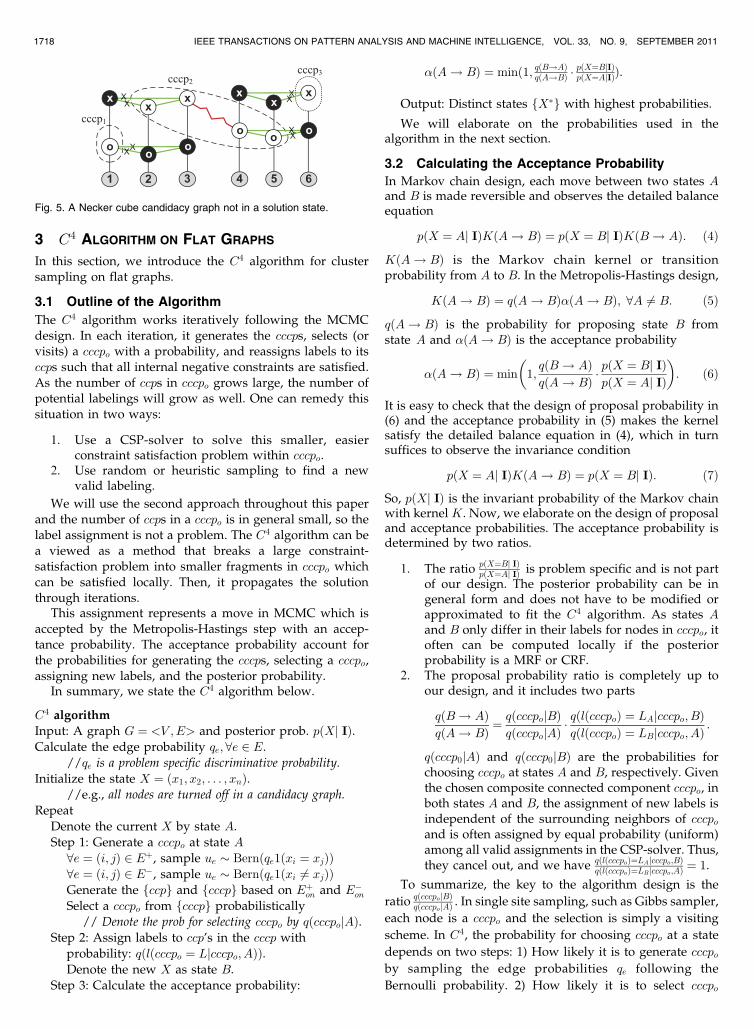
To illustrate the concepts, we show a nonsolution state Xfor the Necker cube in Fig. 5. By turning off some edges(marked with the crosses), we obtain three cccps for thenodes that are currently “on.” In this example, qe ¼ 1 asthese are hard constraints that are inviolable. cccp1 and cccp3

have only one node, and cccp2 has two ccps with four nodes.The algorithm will now arbitrarily select a cccp and updateits values according to its constraints. If it selects either cccp1

or cccp3, then we are one step closer to the solution. If itselects ðcccp2Þ, then all four vertex labels are swapped andwe have reached a solution state and will continue to swapback and forth between the two solutions.


3 C4 ALGORITHM ON FLAT GRAPHS

In this section, we introduce the C4 algorithm for clustersampling on flat graphs.

3.1 Outline of the Algorithm

The C4 algorithm works iteratively following the MCMCdesign. In each iteration, it generates the cccps, selects (orvisits) a cccpo with a probability, and reassigns labels to itsccps such that all internal negative constraints are satisfied.As the number of ccps in cccpo grows large, the number ofpotential labelings will grow as well. One can remedy thissituation in two ways:

1. Use a CSP-solver to solve this smaller, easierconstraint satisfaction problem within cccpo.

2. Use random or heuristic sampling to find a newvalid labeling.

We will use the second approach throughout this paperand the number of ccps in a cccpo is in general small, so thelabel assignment is not a problem. The C4 algorithm can bea viewed as a method that breaks a large constraint-satisfaction problem into smaller fragments in cccpo whichcan be satisfied locally. Then, it propagates the solutionthrough iterations.

This assignment represents a move in MCMC which isaccepted by the Metropolis-Hastings step with an accep-tance probability. The acceptance probability account forthe probabilities for generating the cccps, selecting a cccpo,assigning new labels, and the posterior probability.

In summary, we state the C4 algorithm below.

C4 algorithm

Input: A graph G ¼ <V ;E> and posterior prob. pðXj IÞ.Calculate the edge probability qe; 8e 2 E.

//qe is a problem specific discriminative probability.

Initialize the state X ¼ ðx1; x2; . . . ; xnÞ.//e.g., all nodes are turned off in a candidacy graph.

Repeat

Denote the current X by state A.

Step 1: Generate a cccpo at state A

8e ¼ ði; jÞ 2 Eþ, sample ue � Bernðqe1ðxi ¼ xjÞÞ8e ¼ ði; jÞ 2 E�, sample ue � Bernðqe1ðxi 6¼ xjÞÞGenerate the fccpg and fcccpg based on Eþon and E�onSelect a cccpo from fcccpg probabilistically

// Denote the prob for selecting cccpo by qðcccpojAÞ.Step 2: Assign labels to ccp’s in the cccp with

probability: qðlðcccpo ¼ Ljcccpo; AÞÞ.Denote the new X as state B.

Step 3: Calculate the acceptance probability:

�ðA! BÞ ¼ minð1; qðB!AÞqðA!BÞ �pðX¼BjIÞpðX¼AjIÞÞ.

Output: Distinct states fX�g with highest probabilities.

We will elaborate on the probabilities used in thealgorithm in the next section.

3.2 Calculating the Acceptance Probability

In Markov chain design, each move between two states Aand B is made reversible and observes the detailed balanceequation

pðX ¼ Aj IÞKðA! BÞ ¼ pðX ¼ Bj IÞKðB! AÞ: ð4Þ

KðA! BÞ is the Markov chain kernel or transitionprobability from A to B. In the Metropolis-Hastings design,

KðA! BÞ ¼ qðA! BÞ�ðA! BÞ; 8A 6¼ B: ð5Þ

qðA! BÞ is the probability for proposing state B fromstate A and �ðA! BÞ is the acceptance probability

�ðA! BÞ ¼ min 1;qðB! AÞqðA! BÞ �

pðX ¼ Bj IÞpðX ¼ Aj IÞ

� �: ð6Þ

It is easy to check that the design of proposal probability in(6) and the acceptance probability in (5) makes the kernelsatisfy the detailed balance equation in (4), which in turnsuffices to observe the invariance condition

pðX ¼ Aj IÞKðA! BÞ ¼ pðX ¼ Bj IÞ: ð7Þ

So, pðXj IÞ is the invariant probability of the Markov chainwith kernel K. Now, we elaborate on the design of proposaland acceptance probabilities. The acceptance probability isdetermined by two ratios.

1. The ratio pðX¼Bj IÞpðX¼Aj IÞ is problem specific and is not part

of our design. The posterior probability can be ingeneral form and does not have to be modified orapproximated to fit the C4 algorithm. As states Aand B only differ in their labels for nodes in cccpo, itoften can be computed locally if the posteriorprobability is a MRF or CRF.

2. The proposal probability ratio is completely up toour design, and it includes two parts

qðB! AÞqðA! BÞ ¼

qðcccpojBÞqðcccpojAÞ

� qðlðcccpoÞ ¼ LAjcccpo; BÞqðlðcccpoÞ ¼ LBjcccpo; AÞ

:

qðcccp0jAÞ and qðcccp0jBÞ are the probabilities forchoosing cccpo at states A and B, respectively. Giventhe chosen composite connected component cccpo, inboth states A and B, the assignment of new labels isindependent of the surrounding neighbors of cccpoand is often assigned by equal probability (uniform)among all valid assignments in the CSP-solver. Thus,they cancel out, and we have qðlðcccpoÞ¼LAjcccpo;BÞ

qðlðcccpoÞ¼LBjcccpo;AÞ ¼ 1.

To summarize, the key to the algorithm design is the

ratio qðcccpojBÞqðcccpojAÞ . In single site sampling, such as Gibbs sampler,

each node is a cccpo and the selection is simply a visiting

scheme. In C4, the probability for choosing cccpo at a state

depends on two steps: 1) How likely it is to generate cccpoby sampling the edge probabilities qe following the

Bernoulli probability. 2) How likely it is to select cccpo


Fig. 5. A Necker cube candidacy graph not in a solution state.

from the set of formed fcccpg in states A and B. These

probabilities are hard to compute because there are a vast

amount of partitions of the graph that include a certain

cccpo by turning on/off edges. A partition is a set of cccps

after turning off some edges.Interestingly, the set of all possible partitions in state A

is identical to those in state B, and all of these partitionsmust share the same cut CutðcccpoÞ. That is, in order forcccpo to be a composite connected component, its connec-tions with its neighboring nodes must be turned off. Eventhough the probabilities are in complex form, their ratio issimple and clean due to cancellation. Furthermore, giventhe partition, cccpo is selected with uniform probabilityfrom all possible cccps.

Proposition 1. The proposal probability ratio for selecting cccpoat states A and B is

qðcccp0jBÞqðcccp0jAÞ

¼Q

e2CutðcccpojBÞð1� qeÞQe2CutðcccpojAÞð1� qeÞ

: ð8Þ

We will prove this in the Appendix, which can be found inthe Computer Society Digital Library at http://doi.ieeecomputersociety.org/10.1109/TPAMI.2011.27, in a similarway to the SW-cut method [2].

3.3 Special Case: Potts Model with þ=� Edges

To illustrate C4, we derive it in more detail for a Potts modelwith positive and negative edges. Let X be a random fielddefined on a 2D lattice with discrete states xi 2 f0; 1; 2; . . . ;

L� 1g. Its probability is specified by

pðXÞ ¼ 1

Zexpf�EðXÞg;

EðXÞ ¼X

<i;j>2Eþ��ðxi ¼ xjÞ þ

X<i;j>2E�

��ðxi 6¼ xjÞ;ð9Þ

where � > 0 is a constant. The edge probability will be qe ¼1� e�� for all edges.

Fig. 6a shows an example on a small lattice with L ¼ 2

labels, which is an adjacency graph with position-dependent edges. The states with checkerboard patternswill have highest probabilities. Figs. 6b and 6c show tworeversible states A and B by flipping the label of a cccpoin one step. In this example, cccpo has three ccps,

cccpo ¼ ff2; 5; 6g; f3; 7; 8g; f11; 12gg. The labels of the eight

nodes are reassigned with uniform probability, and this

leads to the difference in the cuts for cccpo at the two states,

CutðcccpojAÞ ¼ fð3; 4Þ; ð4; 8Þ; ð12; 16Þg and CutðcccpojBÞ ¼fð1; 2Þ; ð1; 5Þ; ð5; 9Þ; ð6; 10Þ; ð10; 11Þ; ð11; 15Þg.Proposition 2. The acceptance probability for C4 on the Potts

model is �ðA! BÞ ¼ 1 for any two states with different

labels in cccpo. Therefore, the move is always accepted.

The proof follows two observations. First, the energy terms

inside and outside cccpo are the same for both A and B, and

they differ only at the cuts of cccpo. More precisely, letting

c ¼ jCutðcccpojBÞj � jCutðcccpojAÞ be the difference of sizes

in the two cuts (i.e., c ¼ 3 in our example), it is not too hard

to show that

pðX ¼ Bj IÞpðX ¼ Aj IÞ ¼ e

��c: ð10Þ

Second, we have the proposal probability ratio, following (8):

qðcccp0jBÞqðcccp0jAÞ

¼ ð1� qeÞjCutðcccpojBÞj

ð1� qeÞjCutðcccpojAÞj¼ e�c: ð11Þ

Plugging in the two ratios in (6), we have �ðA! BÞ ¼ 1. In

the literature of SW [10], Edwards and Sokal explain the SW

on Potts model as data augmentation where the edge

variables fueg are treated as auxiliary variables and they

sample fxig and fueg iteratively from a joint probability.

4 EXPERIMENTS ON FLAT GRAPHS

In this section, we test C4’s performance on some flat

graphs (MRF and CRF) in comparison with the Gibbs

sampler [15], SW method [34], ICM, graph cuts [4], and LBP

[21]. We choose classical examples:

1. the Ising/Potts model for MRF,2. line drawing interpretation for constrained-satisfac-

tion problem using candidacy graph,3. scene labeling using CRF, and4. scene interpretation of aerial images.


Fig. 6. The Potts model with negative edges. (a) Minimum energy is a checkerboard pattern. (b) Forming cccps. (c) cccp0 consists of sub-ccps ofpositive edges connected by negative edges.

4.1 Checkerboard Ising Model

We first show the Ising model on a 9� 9 lattice withpositive and negative edges (the Ising model is a specialcase of the Potts model with L ¼ 2 labels). We tested C4

with two parameters settings: 1) � ¼ 1 and thus qe ¼ 0:632;and 2) � ¼ 5 and thus qe ¼ 0:993. In this lattice, we havecreated a checkerboard pattern. We have assigned negativeand positive edges so that blocks of nodes want to be thesame color, but these blocks want to be different colors thantheir neighbors.

Fig. 7 shows a typical initial state to start the algorithm,and two solutions with minimum (i.e., 0) energy. Fig. 8ashows a plot of energy versus time for C4, Gibbs sampler,SW, graph cuts, and LBP. C4 converges second fastest of allfive algorithms in about 10 iterations, behind graph cuts.Belief propagation cannot converge due to the loopiness ofthe graph, and Gibbs sampler and the conventionalSwendsen-Wang cannot quickly satisfy the constraints asthey do not update enough of the space at each iteration.This shows that C4 has a very low burn-in time.

Figs. 8b and 8c show the state visited at each iteration. Weshow the states in three levels: The curve hits the ceiling orfloor for the two minimum energy states, respectively, andthe middle for all other states. Here, we are only comparinggraph cuts, SW, and C4 as they are the only algorithms thatconverge to a solution in a reasonable amount of time. C4

keeps swapping solutions while SW and graph cuts getstuck in their first solution. This is because C4 can groupalong negative edges as well as positive edges to updatelarge portions of the system at once, while Swendsen-Wangis stuck proposing low probability moves over smallerportions of the solution space.

We also compared our results for experiments where � ¼1 and � ¼ 5. Fig. 8c shows the states visited by the samplerover time. In the � ¼ 1 case, it takes longer for C4 toconverge because it cannot form large components withhigh probability. As � gets large, however, C4 very quicklytakes steps in the space toward the solution and can moverapidly between solution states. We have found that anannealing schedule where qe ¼ 1� e��=T and T is adjustedsuch that qe moves from 0 to 1 over the course of theexperiment works quite well too.

We finally compare the estimated marginal beliefs ateach node as computed by each algorithm. LBP computesthese beliefs directly, but we can estimate them for Gibbssampling, SW, and C4 by running each algorithm andrecording the empirical mean at each iteration for each nodegiven the previous states. Fig. 9 shows the belief for one ofthe Ising model sites over time for each of the fouralgorithms. LBP does not converge, so it has a noisyestimate over time and is not plotted for clarity, Gibbs andSW converge to a probability of 1 because they get stuck in asingle solution state, while C4 approaches 0.5 as it keepsflipping between the two states.

4.2 Checkerboard Potts Model with Seven Labels

We ran the same experiment as with the Ising model abovebut this time solved the same checkerboard pattern on aPotts model in which each site could take one of sevenpossible colors (L ¼ 7). In this example, we have a largenumber of equal states (in checkerboard pattern) withminimum energy.

Fig. 10a plots the energy convergence of each algorithmover time. Graph cuts again converges to just one of themany solutions. Unlike in the case of the L ¼ 2 model, SW isable to find multiple solutions this time, as seen in Fig. 10b.Fig. 10c shows the number of distinct states with minimumenergy that have been visited by SW and C4 over time. Wesee that C4 explores more states in a given time limit, which


Fig. 7. The Ising/Potts model with checkerboard constraints and twominimum energy states computed by C4.

Fig. 8. (a) Energy plots of C4, SW, Gibbs sampler, graph cuts, and LBPon the Ising model versus time. (b) and (c) The state (visited by thealgorithms) in time for graph cuts, SW, and C4. Once SW and graph cutshit the first solution, they get stuck, while C4 keeps swapping betweenthe two minimum energy states. C4 results shown for � ¼ 1 and � ¼ 5.

Fig. 9. Comparison of marginal beliefs at a single site of the Ising modelfor Gibbs, SW, and C4. C4 correctly converges toward 0.5, while theother algorithms only find a single solution state. LBP does not convergeand thus has erratic beliefs that we do not show on this plot.

again demonstrates that C4 is more dynamic and thus hasfast mixing time—a crucial measure for the efficiency ofMCMC algorithms. We also compare the case where � ¼ 1versus � ¼ 5. Once again we see that � ¼ 1 does not createstrong enough connections for C4 to move out of localminimum, so it finds roughly as many unique solutions asSwendsen-Wang does (about 13). When � is increased to 5,however, the number skyrockets from 13 to 90. We thus seethat C4 can move around the solution space much morerapidly than other methods when � is high and candiscover a huge number of unique solution states.

4.3 Line Drawing Interpretation

The previous two examples are based on MRF modelswhose edges are position-dependent. Now, we test on linedrawing interpretation on candidacy graph. We use twoclassical examples which have multiple stable interpreta-tions, or solutions: 1) the Necker cube in Fig. 1 that has twointerpretations and 2) a line drawing with double cubes inFig. 11 that has four interpretations. The swapping betweenthese states involves the flipping of 3 or 12 linessimultaneously. Our goal is to test whether the algorithmscan compute the multiple distinct solutions over time.

We adopt a Potts-like model on the candidacy graph.Each line in the line drawing is a node in the Potts model,which can take one of eight line drawing labels indicatingwhether the edge is concave, convex, or a depth boundary.See [33] for an in-depth discussion on labels for consistentline drawings. We add an edge in our candidacy graphbetween any two lines that share a junction. At eachjunction, there are only a small set of valid labels for eachline that are realizable in a 3D world. We add positive edgesbetween pairs of line labels that are consistent with one ofthese junction types, and negative edges between line labels

that are not. Thus, we model the pairwise compatibility ofneighboring line labels given the type of junction they form.

For these experiments, we set � ¼ 2, resulting inqe ¼ 0:865. Figs. 11a and 11c plot the state visited by thealgorithms over time. Once again, we see that C4 canquickly switch between solutions where CSP-solvers orother MCMC methods could get stuck.

4.4 Labeling Man-Made Structures on CRFs

We recreate the experiments in [22], where CRFs werelearned to model man-made structures in images. Fig. 12shows images that are broken into 16� 24 grids andassigned a label xi ¼ f�1;þ1g if they cover a man-madestructure or not. The probability of labeling the sites x givendata y in a CRF is

pðXjY Þ ¼ 1

Zexp

Xi

�ðxi; yÞ þXi

Xj2N i

ðxi; xj; yÞ: ð12Þ

For space, we refer the reader to [22] for more details ofthis model. We simply choose their model so that we cancompare various algorithms on the same representation.The authors use a greedy algorithm (ICM) for inference.

We learned the CRF weights via BFGS [13] using the datafrom [22] and compared inference results using C4 to ICM,LBP, and SW. Edge probabilities were taken from the CRFinteraction potentials. The CRF defines a potential for thecase when two sites have the same label and for when theyhave different labels. If the ratio of these two potentials wasbelow a threshold � , a negative edge was used to connectthe sites to force them to be labeled differently.

Fig. 12 shows the detection results and ground truths. LBPhas very few false positives, but misses huge amounts of thedetection. ICM looks graphically similar to C4, but produces


Fig. 10. (a) Energy plots of C4, SW, Gibbs sampler, and LBP on the Potts model (L ¼ 7) versus time. (b) and (c) The minimum energy states visitedby the SW and C4 algorithms over time. (d) The total number of unique solutions found versus time for SW and C4 with � ¼ 1 and � ¼ 5.

Fig. 11. Experimental results for swapping state between interpretations: (a) States visited by C4 for the Necker cube. (b) A line drawing with outerand inner cubes. (c) States visited by C4 for the double cubes.

significantly more false positives. C4 is able to swap betweenforeground/background fragments in large steps so it canfind blocks of man-made structure more effectively.

Table 1 shows our results as in [22]. We used animplementation for that paper provided by K. Murphy1 thatachieves a higher false positive rate than Hebert’s model.Nevertheless, our goal is not to outperform [22], but toshow that, given the same learned model, C4 can outper-form other inference methods. Here, we see that, forroughly the same false alarm rate, C4 has a higher detectionrate than other algorithms.

4.5 Parsing Aerial Images

In this experiment, we use C4 to parse aerial images. Thisexperiment is an extension of our work from [31]. In [31],aerial images are represented as collections of groups ofobjects, related by statistical appearance constraints. Theseconstraints are learned automatically in an offline phaseprior to inference.

We create our candidacy graph by letting each bottom-up detected window be a vertex in the graph, connected byedges with probabilities proportional to how compatiblethose objects are (we refer to [31] for detailed discussion ofthe energy function). Each candidate can be on or off,indicating whether it is in the current explanation of thescene or not.

Each edge is assigned to be positive or negative andassigned a probability qe of being on by examining theenergy e ¼ �ðxi; xjÞ between its two nodes. If e > t, the edgeis labeled as a negative edge, and if e < t, the edge is labeledas a positive edge, where t is a threshold of the user’schoosing. In our experiments, we let t ¼ 0. In this way, wecreate data-driven edge probabilities and determine posi-tive and negative edge types for C4.

In these experiments, we learned a prior model for likelyobject configurations using labeled aerial images. Object

boundaries were labeled in each image from a set of over50 images. We tested the results on five large aerial imagescollected from Google Earth that were also labeled by handso that we could measure how much C4 improved the finaldetection results. Though we only use five images, eachimage is larger than 1;000� 1;000 pixels and includeshundreds of objects, so one could also think of theevaluation as spanning 125 images of 200� 200 pixels.

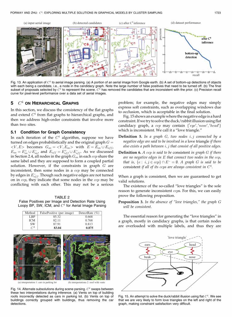
Fig. 13 shows an example of a parsed aerial scene. Thebottom-up detected windows are treated as candidates andmany are false positives. After using C4 minimizing aglobal energy function, however, we are left with the subsetthat best satisfies the constraints of the system. The falsepositive rates are vastly diminished after C4 rules outincompatible proposals. Fig. 13d shows the precision-recallcurve for aerial image object detection using C4 versus justbottom-up cues. We can see that the C4 curve, drawn indashed green, has a much higher precision than the bottom-up detections even as the recall increases.

We also compared the results of using C4 over LBP, ICM,and SW for similar false alarm rates. The results are shownin Table 2.

Fig. 14 shows the true power of C4. Fig. 14a shows aninterpretation of a scene that C4 initially incorrectly labeledas a line of cars in a parking lot, for which it has mistakensome building vents. Because C4 can simultaneously swapthese competing subsolutions, however, we see in Fig. 14bthat, later in the algorithm, C4 has settled on the correctexplanation.


1. http://people.cs.ubc.ca/~murphyk/Software/CRF/crf2D_kumarData.html.

Fig. 12. Man-made structure detection results using a CRF model with LBP, ICM, and C4.

TABLE 1False Positives per Image and Detection Rate Using

Loopy BP, SW, ICM, and C4 for Man-Made Structure Detection

5 C4 ON HIERARCHICAL GRAPHS

In this section, we discuss the consistency of the flat graphs

and extend C4 from flat graphs to hierarchical graphs, andthen we address high-order constraints that involve more

than two sites.

5.1 Condition for Graph Consistency

In each iteration of the C4 algorithm, suppose we haveturned on edges probabilistically and the original graphG ¼<V ;E> becomes Gon ¼ <V ;Eon> with E ¼ Eon [Eoff ,Eon ¼ Eþon [ E�on, and Eoff ¼ Eþoff [ E�off . As we discussedin Section 2.4, all nodes in the graphGon in each ccp share thesame label and they are supposed to form a coupled partialsolution. However, if the constraints in graph G areinconsistent, then some nodes in a ccp may be connectedby edges inE�off . Though such negative edges are not turnedon in ccp, they indicate that some nodes in the ccp may beconflicting with each other. This may not be a serious

problem; for example, the negative edges may simplyexpress soft constraints, such as overlapping windows dueto occlusion, which is acceptable in the final solution.

Fig. 15 shows an example where the negative edge is a hardconstraint. If we try to solve the duck/rabbit illusion using flatcandidacy graph, a ccp may contain f0eye0; 0nose0; 0head0gwhich is inconsistent. We call it a “love triangle.”

Definition 5. In a graph G, two nodes i; j connected by anegative edge are said to be involved in a love triangle if therealso exists a path between i; j that consist of all positive edges.

Definition 6. A ccp is said to be consistent in graph G if thereare no negative edges in E that connect two nodes in the ccp,that is, fe : i; j 2 ccpg \E� ¼ ;. A graph G is said to beconsistent if all of its ccps are always consistent in C4.

When a graph is consistent, then we are guaranteed to getvalid solutions.

The existence of the so-called “love triangles” is the solereason to generate inconsistent ccps. For this, we can easilyprove the following proposition.

Proposition 3. In the absence of “love triangles,” the graph G

will be consistent.

The essential reason for generating the “love triangles” ina graph, mostly in candidacy graphs, is that certain nodesare overloaded with multiple labels, and thus they are


Fig. 13. An application of C4 to aerial image parsing. (a) A portion of an aerial image from Google earth. (b) A set of bottom-up detections of objectswith each being a candidate, i.e., a node in the candidacy graph. Note the large number of false positives that need to be turned off. (b) The finalsubset of proposals selected by C4 to represent the scene. C4 has removed the candidates that are inconsistent with the prior. (c) Precision recallcurve for pixel-level performance over a data set of aerial images.

TABLE 2False Positives per Image and Detection Rate UsingLoopy BP, SW, ICM, and C4 for Aerial Image Parsing

Fig. 14. Alternate subsolutions during scene parsing. C4 swaps betweenthese two interpretations during inference. (a) Vents on top of buildingroofs incorrectly detected as cars in parking lot. (b) Vents on top ofbuildings correctly grouped with buildings, thus removing the cardetections.

Fig. 15. An attempt to solve the duck/rabbit illusion using flat C4. We seethat we are very likely to form love triangles on the left and right of thegraph, making constraint satisfaction very difficult.

coupled with conflicting nodes. For example, the node“eye” should be either a “rabbit eye” or a “duck eye” and itshould be split into two conflicting candidates connected byan negative edge. This way it can eliminate the “lovetriangle.” Fig. 16 illustrates that we can remove the lovetriangle by splitting node 1 into nodes 1 and 10, and thuswe will have consistent ccp.

5.2 Formulation of Hierarchical C4

One other common issue that we need to address is higherorder constraints that involve more than two nodes. Fig. 17shows a hierarchical graph representation for the duck/rabbit illusion. This is a candidacy graph with two layers.The top layer contains two hidden candidate hypotheses:“duck” and “rabbit.” The two nodes are decomposed intothree parts in layer 1, respectively, and thus impose high-order constraints between them. Now, the hypotheses forparts are specifically for “duck.eye,” “rabbit.eye,” etc. Thenegative edge connecting the two object nodes is inheritedfrom their overlapping children.

This hierarchical candidacy graph is constructed on-the-fly with nodes being generated by multiple bottom-updetection and binding processes as well as top-downprediction processes. We refer to a recent paper by Wuand Zhu [39] for the various bottom-up/top-down pro-cesses in object parsing. In this graph, positive and negativeedges are added between nodes on the same layers in a wayidentical to the flat candidacy graph, while the vertical linksbetween parent-child nodes are deterministic.

By turning on/off the positive and negative edgesprobabilistically at each layer, C4 obtains ccps and cccps asin the flat candidacy graphs. In this case, a ccp contains aset of nodes that are coupled in both horizontal andvertical directions and thus represents a partial parse tree.A cccp contains multiple competing parse trees, which willbe swapped in a single step. For example, the left panel in

Fig. 17 shows two ccps for the duck and rabbit, respec-tively, which are connected with negative edges in the

candidacy graph.This hierarchical representation can also eliminate the

inconsistency caused by overloaded labels. That is, if a

certain part is shared by multiple object or object instances,we need to create multiple instances as nodes in the

hierarchical candidacy graph.

5.3 Experiments on Hierarchical C4

To demonstrate the advantages of hierarchical C4 overflat C4, we present two experiments 1) interpreting theduck/rabbit illusion, and 2) finding configurations of objectparts amid extremely high noise.

1. Experiment on hierarchical duck/rabbit illusion.As referenced above, C4 on the flat candidacy graphin Fig. 15 creates two love triangles. The top panel ofFig. 18 shows the results of flat C4 on the duck/rabbit illusion. C4 continuously swaps between twostates, but the two states either have all nodes on orall nodes off, neither of which are valid solutions.The bottom panel of Fig. 18 shows the results ofapplying hierarchical C4 to the duck/rabbit illusion.We defined a tree for the duck/rabbit illusionconsisting of either a duck, fbeak; eye; duckheadg or arabbit fears; eye; rabbitheadg. As a result, the algo-rithm instantly finds both solutions and thenproceeds to swap between them uniformly. Theseresults show that hierarchical C4 can help guide thealgorithm to more robust solutions and negatesthe effects of love triangles.


Fig. 16. Breaking the “love triangle” in a candidacy graph.

Fig. 17. An attempt to solve the duck/rabbit illusion using hierarchical C4.The trees define which parts comprise each object. Nodes are groupedaccording to these trees, creating higher level nodes. The higher levelnodes inherit the negative constraints.

Fig. 18. (Top panel) Flat C4 results on the duck/rabbit illusion. C4 swapsbetween two impossible states due to love triangles. (Bottom panel)Hierarchical C4 results on the duck/rabbit solution. C4 now swapsuniformly between the two correct solutions.

2. Experiments on object parsing. A problem thatoften appears in computer science is the problem offinding the optimal subset from a larger set of itemsthat minimizes some energy function. For example,in the star model [12], many instances of each objectpart may be detected in the image. However, ouralgorithm should find the subset (or subsets) of thesedetections that creates the highest probability con-figuration. This is a combinatorially hard problem asthe number of solutions grows exponentially in thenumber of detections, so heuristic approaches areusually proposed to deal with this situation. One canuse dynamic programming for inferring star models,but these require that the root part be present, whichour algorithm does not. Hierarchical C4 is ideallysuited for this problem as it can use local edgeconstraints and hierarchical grouping to guide itssearch through large sets of detections to find themost likely solutions.

In this experiment, we learned a star model for fourcategories of objects: “side car,” “front car,” “teapot,” and“clock.” We collected 25-50 images from the Lotus Hill DataSet [38] for each of the categories, which include the truelabeled parts of each object. We then added 50 falsedetection at random orientations, scales, and positions, foreach part to serve as distractors, as shown in Fig. 19. Thegoal is to see if the algorithms can identify the true groundtruth configuration amidst a huge number of distractors. Ifso, then such an algorithm could thrive when we have weakpart detectors but strong geometric information. If we onlyconsidered configurations of four parts, finding the optimalconfiguration would require exhaustively searching

64,684,950 configurations, which quickly becomes intract-able when considering larger configurations or moredetections.

Fig. 19 shows that ICM and Swendsen-Wang findcompletely unreasonable solutions. Flat C4 does not findthe correct solution although it does find a set of parts thatlook similar to a teapot. Hierarchical C4, on the other hand,quickly converges to the true solution amid the myriadother possible part combinations available.

Fig. 21 shows the results of other signal-from-noiseimages that were generated as above. We show the results

divided into roughly three categories: good, medium, and

bad results. We see that hierarchical C4 gets mostly good

results, while ICM gets entirely bad results.Fig. 22 shows the energy of the system over time for the

four algorithms we tested. Not only does hierarchical C4

achieve a minimum energy almost instantaneously, but

both hierarchical C4 and flat C4 are able to achieve lower

energy minimums than the other methods. This improve-

ment applies to graph cuts as well, which, as mentioned, are

not shown here because no implementation we found wasable to converge in the presence of love triangles. This result

shows Hierarchical C4’s ability to quickly find deeper

energy minima than competing approaches.


Fig. 19. Hierarchical C4 for detecting signal from noise. A huge set ofdistractors is added over a true parse of an object. Using a spatialmodel, C4 can find the best subset while other algorithms cannot.

Fig. 20. True positive, false positive, true negative, and false negativerates for object part detection on the teapot category when usingdifferent negative edge thresholds. The plots all have a minimum/maximum near 1e-7.

Fig. 21. Examples of good/medium/bad results for Hierarchical C4, Flat C4, Swendsen-Wang cuts, and ICM. The graphs to the right show theproportion of the testing images that belonged to each ranking according to algorithm.

We also tested our negative edge selection criteria. Weuse a threshold the pairwise probabilities computed by thestar model to create negative and positive edges. We hadempirically arrived at a threshold between positive andnegative edges of 1e-7. Fig. 20 shows the true positive, falsepositive, true negative, and false negative rates for differentthresholds (on a log scale). We can see that 1e-7 is a goodcutoff probability as it produces a clear peak in the plots(note that all individual edge probabilities are quite low inour star models). We propose to look at general heuristicsfor negative edge creation in future work.

These results show the power of Hierarchical C4 forquickly finding minimal energy subsets and swappingbetween equally or nearly equally likely solutions oncefound, where as similar methods (Swendsen-Wang, ICM,Graph Cuts) fail to even find a viable solution.

6 DISCUSSION

In this paper, we presented C4, an algorithm that canhandle complex energy minimization tasks with soft andhard constraints. By breaking a large CSP into smaller sub-CSPs probabilistically, C4 can quickly find multiple solu-tions and switch between them effectively. This combina-tion of cluster sampling and constraint-satisfactiontechniques allows C4 to achieve a fast mixing time,outperforming single-site samplers, and techniques-likebelief propagation on existing problems. This novel algo-rithm can sample from arbitrary posteriors and is thusapplicable to general graphical models, including MRFsand CRFs. In addition, we were able to use a hierarchicalprior to guide our search to avoid frustrations in the graphand thus achieve richer and more accurate results than justby using Flat C4 alone.

In this paper, we applied C4 to a number of simpleapplication for illustration purpose. In two related papersby the authors’ group, the C4 algorithm was applied tolayered graph matching [24] and aerial image parsing [31]with state-of-the-art results. In ongoing work, we areextending C4 for scene labeling, integrating object parsing,and scene segmentation.

ACKNOWLEDGMENTS

This work was partially supported by US National ScienceFoundation (NSF) IIS grant 1018751 and US Office of Naval

Research MURI grant N000141010933. The authors would

also like to acknowledge the support of the LHI data set

[38]. Work done at LHI was supported by 863 grant

2009AA01Z331 and NSFC 90920009. J. Porway was a PhD

student with the Department of Statistics, University of

California, Los Angeles (UCLA) when this paper was

submitted.

REFERENCES

[1] K.R. Apt, “The Essence of Constraint Propagation,” TheoreticalComputer Science, vol. 221, pp. 179-210, 1999.

[2] A. Barbu and S.C. Zhu, “Generalizing Swendsen-Wang toSampling Arbitrary Posterior Probabilities,” IEEE Trans. PatternAnalysis and Machine Intelligence, vol. 27, no. 8, pp. 1239-1253, Aug.2005.

[3] J. Besag, “On the Statistical Analysis of Dirty Pictures,” J. RoyalStatistical Soc. Series B, vol. 48, no. 3, pp. 259-302, 1986.

[4] Y. Boykov, O. Veksler, and R. Zabih, “Fast Approximate EnergyMinimization via Graph Cuts,” IEEE Trans. Pattern Analysis andMachine Intelligence, vol. 23, no. 11, pp. 1222-1239, Nov. 2001.

[5] A. Braunstein, M. Mzard, and R. Zecchina, “Survey Propagation:An Algorithm for Satisfiability,” Random Structures and Algorithms,vol. 27, pp. 201-226, 2005.

[6] H. Chui and A. Rangarajan, “A New Point Matching Algorithmfor Non-Rigid Registration,” Computer Vision and Image Under-standing, vol. 89, no. 2, pp. 114-141, 2003.

[7] C. Cooper and A. Frieze, “Mixing Properties of the Swendsen-Wang Process in Classes of Graphs,” Random Structures andAlgorithms, vol. 15, nos. 3/4, pp. 242-261, 1999.

[8] T. Cormen, C.E. Leiserson, R.L. Rivest, and C. Stein, Introduction toAlgorithms, second ed. MIT Press/McGraw-Hill, 2001.

[9] F. Dellaert, S. Seitz, C. Thorpe, and S. Thrun, “Feature Corre-spondence: A Markov Chain Monte Carlo Approach,” Advances inNeural Information Processing Systems, vol. 13, MIT Press, pp. 852-858, 2001.

[10] R. Edwards and A. Sokal, “Generalization of the Fortuin-Kasteleyn-Swendsen-Wang Representation and Monte CarloAlgorithm,” Physical Rev. Letters, vol. 38, pp. 2009-2012, 1988.

[11] P.F. Felzenszwalb and J.D. Schwartz, “Hierarchical Matching ofDeformable Shapes,” Proc. IEEE Conf. Computer Vision and PatternRecognition, 2007.

[12] R. Fergus, P. Perona, and A. Zisserman, “A Sparse ObjectCategory Model for Efficient Learning and Exhaustive Recogni-tion,” Proc. IEEE Conf. Computer Vision and Pattern Recognition,2005.

[13] R. Fletcher, “A New Approach to Variable Metric Algorithms,”Computer J., vol. 13, pp. 317-322, 1970.

[14] A. Gelman, J.B. Carlin, H.S. Stern, and D.B. Rubin, Bayesian DataAnalysis. second ed, chapter 5. Chapman and Hall/CRC, 2004.

[15] S. Geman and D. Geman, “Stochastic Relaxation, Gibbs Distribu-tions and the Bayesian Restoration of Images,” IEEE Trans. PatternAnalysis and Machine Intelligence, vol. 6, no. 6, pp. 721-741, Nov.1984.

[16] V.K. Gore and M.R. Jerrum, “The Swendsen-Wang Process DoesNot Always Mix Rapidly,” Proc. 29th Ann. ACM Symp. Theory ofComputing, pp. 674-681, 1997.

[17] P. Green, “Reversible Jump Markov Chain Monte CarloComputation and Bayesian Model Determination,” Biometrika,vol. 82, pp. 711-732, 1995.

[18] U. Grenander and M.I. Miller, “Representations of Knowledge inComplex Systems,” J. Royal Statistical Soc. Series B, vol. 56, no. 4,pp. 549-603, 1994.

[19] D.A. Huffman, “Impossible Objects as Nonsense Sentences,”Machine Intelligence, vol. 8, pp. 475-492, 1971.

[20] V. Kolmogorov and C. Rother, “Minimizing NonsubmodularFunctions with Graph Cuts-A Review,” IEEE Trans. PatternAnalysis and Machine Intelligence, vol. 29, no. 7, pp. 1274-1279, July2007.

[21] M. Kumar and P. Torr, “Fast Memory-Efficient Generalized BeliefPropagation,” Lecture Notes in Computer Science, Springer-Verlag,2006.

[22] S. Kumar and M. Hebert, “Man-Made Structure Detection inNatural Images Using a Causal Multiscale Random Field,” Proc.IEEE Conf. Computer Vision and Pattern Recognition, 2003.


Fig. 22. Plots of energy over time for Hierarchical C4, Flat C4,Swendsen-Wang cuts, and ICM. Not only does Hierarchical C4

converge fastest of all of the algorithms, but it achieves a lower energythan the other methods.

[23] J. Lafferty and F. Pereira, “Conditional Random Fields: Probabil-istic Models for Segmenting and Labeling Sequence Data,” Proc.Int’l Conf. Machine Learning, 2001.

[24] L. Lin, K. Zeng, X.B. Liu, and S.C. Zhu, “Layered Graph Matchingby Composite Clustering with Collaborative and CompetitiveInteractions,” Proc. IEEE Conf. Computer Vision and PatternRecognition, 2009.

[25] J. Liu, Monte Carlo Strategies in Scientific Computing. Springer,2001.

[26] J. Liu, W.H. Wong, and A. Kong, “Correlation Structure andConvergence Rate of the Gibbs Sampler with Various Scans,”J. Royal Statistical Soc. Series B, vol. 57, pp. 157-169, 1995.

[27] A.K. Mackworth, “Interpreting Pictures of Polyhedral Scenes,”Artificial Intelligence, vol. 4, no. 2, pp. 121-137, 1973.

[28] A.K. Mackworth, “Consistency in Networks of Relations,”Artificial Intelligence, vol. 8, pp. 99-118, 1977.

[29] S. Oh, J. Rehg, T. Balch, and F. Dellaert, “Learning and Inference inParametric Switching Linear Dynamical Systems,” Proc. IEEE Int’lConf. Computer Vision, vol. 2, pp. 1161-1168, 2005.

[30] J. Pearl, Heuristics:Intelligent Search Strategies for Computer ProblemSolving, Addison-Wesley Longman Publishing, 1984.

[31] J. Porway, K. Wang, and S.C. Zhu, “A Hierarchical and ContextualModel for Aerial Image Understanding,” Int’l J. Computer Vision,vol. 88, no. 2, pp. 254-283, 2010.

[32] A. Rosenfeld, R.A. Hummel, and S.W. Zucker, “Scene Labeling byRelaxation Operations,” IEEE Trans. Systems, Man, and Cybernetics,vol. 6, no. 6, pp. 420-433, June 1976.

[33] K. Sugihara, Machine Interpretation of Line Drawings. MIT Press,1986.

[34] R.H. Swendsen and J.S. Wang, “Nonuniversal Critical Dynamicsin Monte Carlo Simulations,” Physical Rev. Letters, vol. 58, no. 2,pp. 86-88, 1987.

[35] Z. Tu and S.C. Zhu, “Image Segmentation by Data-Driven MarkovChain Monte Carlo,” IEEE Trans. Pattern Analysis and MachineIntelligence, vol. 24, no. 5, pp. 657-673, May 2002.

[36] A. Torralba, K. Murphy, and W. Freeman, “Object Detection,”Proc. IEEE Conf. Computer Vision and Pattern Recognition, 2004.

[37] Y. Weiss, “Correctness of Local Probability Propagation inGraphical Models with Loops,” Neural Computation, vol. 12, no. 1,pp. 1-41, 2000.

[38] B. Yao, M. Yang, and S.C. Zhu, “Introduction to a Large-ScaleGeneral Purpose Ground Truth Database: Methodology, Annota-tion Tools and Benchmarks,” Proc. Int’l Conf. Energy MinimizationMethods in Computer Vision and Pattern Recognition, 2007.

[39] T.F. Wu and S.C. Zhu, “A Numeric Study of the Bottom-Up andTop-Down Inference Processes in And-Or Graphs,” Int’l J.Computer Vision, 2010.

[40] S.C. Zhu and D. Mumford, “A Stochastic Grammar of Images,”Foundations and Trends in Computer Graphics and Vision, vol. 2,no. 4, pp. 259-362, 2006.

Jake Porway received the BS degree incomputer science from Columbia University in2000 with a focus on intelligent systems, and theMS and PhD degrees in statistics from theUniversity of California, Los Angeles (UCLA) in2005 and 2010, respectively. During his PhDcareer, he worked in the CIVS lab at UCLA,where his research focused on probabilisticgrammar models for object recognition inimages and video, Bayesian methods for in-

ference in graphical models, and unsupervised and semi-supervisedmethods for automated learning. At the time of this publication, he isworking as the data scientist for the New York Times R&D division and isexamining the role of big data in modern machine learning applications.He is a student member of the IEEE.

Song Chun Zhu received the BS degree fromthe University of Science and Technology ofChina in 1991 and the MS and PhD degreesfrom Harvard University in 1994 and 1996,respectively. He is currently a professor withthe Department of Statistics and the Departmentof Computer Science at the University ofCalifornia, Los Angeles (UCLA). Before joiningUCLA, he was a postdoctoral researcher in theDivision of Applied Math at Brown University

from 1996 to 1997, a lecturer in the Department of Computer Science atStanford University from 1997 to 1998, and an assistant professor ofcomputer science at The Ohio State University from 1998 to 2002. Hisresearch interests include computer vision and learning, statisticalmodeling, and stochastic computing. He has published more than100 papers in computer vision. He has received a number of honors,including the David Marr Prize in 2003 with Z. Tu et al., theJ.K. Aggarwal prize from the International Association of PatternRecognition in 2008, the Marr Prize honorary nominations in 1999 and2007 with Y.N. Wu et al., a Sloan Fellowship in Computer Science in2001, a US National Science Foundation Early Career DevelopmentAward in 2001, and a US Office of Naval Research Young InvestigatorAward in 2001. In 2005, he founded, with friends, the Lotus Hill Institutefor Computer Vision and Information Science in China as a nonprofitresearch organization (www.lotushill.org). He is a fellow of the IEEE.

. For more information on this or any other computing topic,please visit our Digital Library at www.computer.org/publications/dlib.


IEEE TRANSACTIONS ON PATTERN ANALYSIS AND …sczhu/papers/prints/C4_PAMI.pdf · C4: Exploring...

Documents

Transcript of IEEE TRANSACTIONS ON PATTERN ANALYSIS AND …sczhu/papers/prints/C4_PAMI.pdf · C4: Exploring...