Identifying the Elasticity of Substitution with

Biased Technical Change

Miguel A. León-Ledesma‡, Peter McAdam§,∗ and Alpo Willman§

‡University of Kent, §European Central Bank.

30th September 2008

Abstract

Despite being critical parameters in many economic �elds, the receivedwisdom, in theoretical and empirical literatures, states that joint identi�ca-tion of the elasticity of capital-labor substitution and technical bias is infea-sible. This paper challenges that pessimistic interpretation. Putting the newapproach of �normalized� production functions at the heart of a Monte Carloanalysis we identify the conditions under which identi�cation is feasible androbust. The key result is that the jointly modeling the production functionand �rst-order conditions is superior to single-equation approaches in termsof robustly capturing production and technical parameters, especially whenmerged with "normalization". Our results will have fundamental implica-tions for production-function estimation under non-neutral technical change,for understanding the empirical relevance of normalization and the variabilityunderlying past empirical studies.JEL Classi�cation: C22, E23, O30, 051.Keywords: Constant Elasticity of Substitution, Factor-Augmenting Techni-cal Change, Normalization, Factor Income share, Identi�cation, Monte Carlo.

∗Corresponding author: peter.mcadam@ecb.int, Research Dept., ECB, Kaiserstr. 29, D-60311Frankfurt am Main, Germany. Tel: +.49.69.13.44.6434.

1 Introduction

The elasticity of substitution between capital and labor and the direction of technical

change are critical parameters in many areas of economics; almost all macro or

growths model embody some explicit production technology. How useful such models

prove to be then on the appropriateness of their technical assumptions.

Why do these parameter matter so much? The value of the substitution elas-

ticity, for example, has been linked to di�erences in international factor returns

and convergence (e.g., Klump and Preissler (2000), Mankiw (1995)); movements

in income shares (Blanchard (1997), Caballero and Hammour (1998)), trade and

development patterns (e.g., Jones (1965); Du�y and Papageorgiou (2000)); the ef-

fectiveness of employment-creation policies (Rowthorn (1999)) etc. Recent work on

�normalized�1 Constant Elasticity of Substitution (CES) functions has also formal-

ized a correspondence between substitution possibilities and growth (La Grandville

(1989), Klump and de La Grandville (2000), La Grandville and Solow (2008))2. The

nature of technical change, on the other hand, matters for characterizing the welfare

consequences of new technologies (Marquetti (2003)); labor-market inequality and

skills premia (Acemoglu (2002b)); the evolution of factor income shares (Kennedy

(1964), Acemoglu (2003)) etc. Moreover, the interdependency between substitution

possibilities and technical change has also sparked several interesting debates: e.g.,

on relating constellations of the substitution elasticity and technical change with

the shape of the (local and global) production function, (e.g., Acemoglu (2003),

Jones (2005)), and in accounting for medium-run departures from balanced growth

(McAdam and Willman (2008)) etc.

Despite the importance of these debates, the received wisdom � in both theoretical

and empirical literatures � suggests that identifying the elasticity of substitution

with non-neutral technical change is largely infeasible. If so, this would render such

debates indeterminate.

First, consider theoretical arguments. If production is Cobb-Douglas (i.e., uni-

tary substitution), then technological progress degenerates to the Hicks-Neutral rep-

resentation. In the case of a non-unitary substitution elasticity, in turn, Diamond

et al. (1978) asserted that the elasticity and biased technical change cannot be si-

1Normalization essentially implies representing the production function in consistent indexednumber form.

2This is termed the �de La Grandville Hypothesis� following La Grandville (1989) and Yuhn(1991). Also, in an earlier contribution, Solow (1956) and Pitchford (1960) showed in the neoclassi-cal growth model that a CES function with an elasticity of substitution greater than one generatessustained growth (even without technical progress).

1

multaneously identi�ed. To counter this �impossibility theorem� researchers usually

impose speci�c functional forms for technical progress, e.g., a deterministic (expo-

nential) function and restrictive assumptions about technological progress (e.g. im-

posing Harrod Neutrality). However, arbitrary ex-ante identi�cation schemes risk

spurious ex-post inference. Antràs (2004), for instance, suggested that the popular

assumption of Hicks-neutral technical progress, coupled with relatively stable factor

shares and rising capital deepening biases results towards Cobb-Douglas.

On the empirical side, despite the huge e�orts devoted to their identi�cation, lim-

ited consensus has emerged on the value of the substitution elasticity and arguably

less on the nature of technical change. This doubtless re�ects many practical data

problems (e.g., outliers, uncertain auto-correlation, structural breaks, quality im-

provements, measurement errors etc) as well as a priori modeling choices (as just

discussed) and the performance of various estimators. An added problem, however,

is that often the predictions of di�erent elasticity and technical change combinations

can have similar implications for variables of interest, such as factor income shares

and factor ratios. Notwithstanding, whether factor income movements are driven

by high or low substitution elasticities and with di�erent combinations of techni-

cal change is profoundly important in terms of their di�erent implications for, e.g.,

growth accounting, inequality, calibration in business-cycle models, public policy

issues etc.

It is legitimate to wonder if standard techniques can separate these e�ects. It is

this key question that we address. To do so, we employ Monte Carlo sampling tech-

niques. Despite their natural appeal in uncovering CES properties, there have been

relatively few such studies; re�ecting, arguably, the numerical complexity involved

and weak results typically reported. Some studies were, for instance, e�ectively only

interested in uncovering single production parameters (e.g., Maddala and Kadane

(1966)), leaving researchers unclear as to overall performance. However, more elab-

orate studies (e.g., Kumar and Gapinski (1974); Thursby (1980)) suggested joint

parameter identi�cation was highly problematic (the substitution elasticity seemed

especially challenging yielding sometimes highly implausible �rst and second mo-

ments).

Our paper o�ers a signi�cant improvement over these earlier studies. First, in

contrast to the actual US data studies of Kumar and Gapinski (1974) and Thursby

(1980), we employ a carefully constructed, pre-determined data generation process

(DGP). Knowing the exact nature of the data, we can attribute all di�erences in

parameter estimates to the technique used. Thus, we can rank di�erent approaches

2

in terms of their ability to replicate the known DGP and explain that ranking.

Second, we consider a more comprehensive range of estimation forms and types

than previously (single-equation, system, linear, non-linear, linearized). We also

examine a rich source of robustness issues: auto-correlated errors, sample size, the

e�ect of di�erent initial conditions, etc. Finally, we take �normalization� seriously

(La Grandville (1989), Klump and de La Grandville (2000)). We �nd that normal-

ization besides o�ering several theoretically-consistent advantages, also improves

empirical identi�cation.

Our �ndings are that single equation approaches are largely unsuitable for jointly

uncovering technical characteristics. This applies also to our generalized form of

the Kmenta approximation (for which we derive some weak technical identi�cation

results). Moreover, direct estimation of the non-linear CES does not alleviate iden-

ti�cation problems (especially so for high elasticity cases). The key result is the

superiority of the system approach (i.e., jointly modeling the production function

and �rst-order conditions) in terms of robustly capturing production and technical

parameters. This approach further allows us to highlight the empirical advantages

of �normalization�.

The paper proceeds as follows. Section 2 reviews some relevant technical con-

cepts of the CES function with technical change. The subsequent section brie�y

appraises existing empirical studies and their apparent lack of robustness. Section 4

discusses the concept of normalization. Section 5 explains the di�erent approaches

for estimating the production function and technical change used, whilst the subse-

quent section elaborates on the Monte Carlo. Sections 7 and 8 present our results

and robustness extensions. Section 9 concludes.

2 Background: The CES Production Function and

Technical Change.

The CES production function � a special type of function rooted in the mathematical

theory of elementary mean values (Hardy et al. (1934), p. 13 �.) � was introduced

into economics by Dickinson (1955) and Solow (1956) and further pioneered by

Pitchford (1960), Arrow et al. (1961), David and van de Klundert (1965) and others.

It takes the form:

F(ΓK

t Kt, ΓNt Nt

)= C

[π

(ΓK

t Kt

)σ−1σ + (1− π)

(ΓN

t Nt

)σ−1σ

] σσ−1

(1)

3

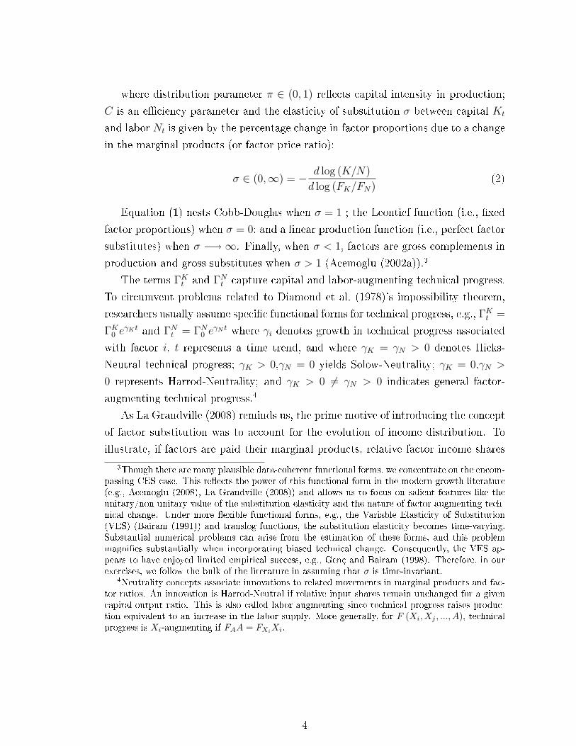
where distribution parameter π ∈ (0, 1) re�ects capital intensity in production;

C is an e�ciency parameter and the elasticity of substitution σ between capital Kt

and labor Nt is given by the percentage change in factor proportions due to a change

in the marginal products (or factor price ratio):

σ ∈ (0,∞) = − d log (K/N)

d log (FK/FN)(2)

Equation (1) nests Cobb-Douglas when σ = 1 ; the Leontief function (i.e., �xed

factor proportions) when σ = 0; and a linear production function (i.e., perfect factor

substitutes) when σ −→ ∞. Finally, when σ < 1, factors are gross complements in

production and gross substitutes when σ > 1 (Acemoglu (2002a)).3

The terms ΓKt and ΓN

t capture capital and labor-augmenting technical progress.

To circumvent problems related to Diamond et al. (1978)'s impossibility theorem,

researchers usually assume speci�c functional forms for technical progress, e.g., ΓKt =

ΓK0 eγKt and ΓN

t = ΓN0 eγN t where γi denotes growth in technical progress associated

with factor i, t represents a time trend, and where γK = γN > 0 denotes Hicks-

Neutral technical progress; γK > 0,γN = 0 yields Solow-Neutrality; γK = 0,γN >

0 represents Harrod-Neutrality; and γK > 0 6= γN > 0 indicates general factor-

augmenting technical progress.4

As La Grandville (2008) reminds us, the prime motive of introducing the concept

of factor substitution was to account for the evolution of income distribution. To

illustrate, if factors are paid their marginal products, relative factor income shares

3Though there are many plausible data-coherent functional forms, we concentrate on the encom-passing CES case. This re�ects the power of this functional form in the modern growth literature(e.g., Acemoglu (2008), La Grandville (2008)) and allows us to focus on salient features like theunitary/non-unitary value of the substitution elasticity and the nature of factor-augmenting tech-nical change. Under more �exible functional forms, e.g., the Variable Elasticity of Substitution(VES) (Bairam (1991)) and translog functions, the substitution elasticity becomes time-varying.Substantial numerical problems can arise from the estimation of these forms, and this problemmagni�es substantially when incorporating biased technical change. Consequently, the VES ap-pears to have enjoyed limited empirical success, e.g., Genç and Bairam (1998). Therefore, in ourexercises, we follow the bulk of the literature in assuming that σ is time-invariant.

4Neutrality concepts associate innovations to related movements in marginal products and fac-tor ratios. An innovation is Harrod-Neutral if relative input shares remain unchanged for a givencapital-output ratio. This is also called labor-augmenting since technical progress raises produc-tion equivalent to an increase in the labor supply. More generally, for F (Xi, Xj , ..., A), technicalprogress is Xi-augmenting if FAA = FXi

Xi.

4

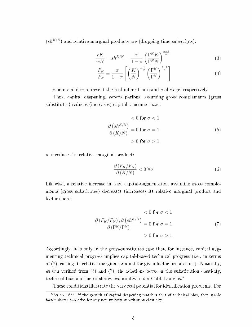
(shK/N) and relative marginal products are (dropping time subscripts):

rK

wN= shK/N =

π

1− π

(ΓKK

ΓNN

)σ−1σ

(3)

FK

FN

=π

1− π

[(K

N

)− 1σ

(ΓK

ΓN

)σ−1σ

](4)

where r and w represent the real interest rate and real wage, respectively.

Thus, capital deepening, ceteris paribus, assuming gross complements (gross

substitutes) reduces (increases) capital's income share:

< 0 for σ < 1

∂(shK/N

)∂ (K/N)

= 0 for σ = 1 (5)

> 0 for σ > 1

and reduces its relative marginal product:

∂ (FK/FN)

∂ (K/N)< 0 ∀σ (6)

Likewise, a relative increase in, say, capital-augmentation assuming gross comple-

ments (gross substitutes) decreases (increases) its relative marginal product and

factor share:

< 0 for σ < 1

∂ (FK/FN) , ∂(shK/N

)∂ (ΓK/ΓN)

= 0 for σ = 1 (7)

> 0 for σ > 1

Accordingly, it is only in the gross-substitutes case that, for instance, capital aug-

menting technical progress implies capital-biased technical progress (i.e., in terms

of (7), raising its relative marginal product for given factor proportions). Naturally,

as can veri�ed from (5) and (7), the relations between the substitution elasticity,

technical bias and factor shares evaporates under Cobb-Douglas.5

These conditions illustrate the very real potential for identi�cation problems. For

5As an aside: if the growth of capital deepening matches that of technical bias, then stablefactor shares can arise for any non-unitary substitution elasticity.

5

example a rise in the labor share could be equally well explained by a rise [or fall]

in capital deepening in e�ciency units depending on whether production exhibits

gross-complements [or gross substitutes]. Failure to properly identify the nature of

the substitution elasticity in the �rst instance will thus seriously deteriorate inference

on biased technical change on a given dataset.

3 Empirical Studies on the Substitution Elasticity

and Technical Bias

Despite the centrality of the substitution elasticity and technical biases in many

areas of economics, and the huge e�orts devoted to their identi�cation, there seems

little empirical consensus on their value and nature. Table 1 summarizes some well-

known empirical studies for the US: we observe a variety of augmentation forms and

elasticity values.6 Despite its pervasive use, we observe limited support for Cobb-

Douglas and for above-unitary substitution elasticities in general.

We brie�y review reasons for such heterogeneity in results. This will also help

to clarify our contribution.

(a) Data quality and data consistency.

Several papers (e.g., Berndt (1976), Antràs (2004), Klump et al. (2007)) put a

strong emphasis on the selection of high-quality, consistent data. Problems never-

theless remain endemic to production function estimation: e.g., the correct mea-

surement of the user cost and capital income, the possible use of quality-adjusted

measures for factor inputs, neglect of capital depreciation and the aggregate mark-

up, the treatment of indirect taxes, assumptions about self-employed labor income,

measurement of capacity utilization rates, and so on.

6The substitution elasticity tends to be greater when estimated from aggregate time series thanfrom micro (�rm, industry) cross-section/panel studies.

6

(b) Choice of estimating equation7

On the conceptual side there is the problem of how exactly the production pa-

rameters are to be estimated. Single equation, two- and three-equation system ap-

proaches are competing. Single equation estimates usually concentrate either on the

production function or on the one of the �rst-order conditions of pro�t maximization,

whilst system approaches combine them exploiting cross-equation restrictions.

The estimation of the production function alone is generally only accomplished

with quite restrictive assumptions about the nature of technological progress. Antràs

(2004), for instance, argued that the popular assumption of Hicks-neutral technical

progress, coupled with a relatively stable factor share and rising long-run capi-

tal deepening biases results towards Cobb-Douglas (famously advocated by Berndt

(1976) for US manufacturing). Furthermore, the elasticity of substitution estimated

from the �rst-order condition with respect to labor seems to be systematically higher

than that with respect to capital.8 Single equation estimates (based on factor de-

mand functions) may be systematically biased, since factor inputs depend on rela-

tive factor prices that again depend on relative factor inputs (see David and van de

Klundert (1965), p. 369; Willman (2002)).

Two-equation systems that estimate demand functions for both input factors as

in Berthold et al. (2002) should alleviate such a systematic simultaneous equation

bias. However, since two-equation systems usually do not explicitly estimate a pro-

duction function (with the nature of technological progress restricted by a priori

assumptions), identi�cation remains problematic. The bene�t of a three-equation

System is that it treats the �rst-order conditions of pro�t maximizing jointly, con-

taining cross-equation parameter constraints, which may facilitate the joint identi-

�cation of the technical parameters.

7Although an important issue in itself, we do not consider the e�ect of adjustment costs inidentifying production and technology parameters (e.g., Caballero (1994)). To pursue this wouldrequire agreement on the functional form of such adjustment costs and distributed lag structure forfactor demands and technology. As Chirinko (2008) notes, most studies of production parametersare, as here, performed using long-run or frictionless concepts and are generally to be preferred forcapturing deep production characteristics.

8This is also our �nding. We rationalize this as being due to the di�erential shock processon capital and labor returns (see section 7). Discussing this in a dynamic setting, Berndt (1991)suggests it also relates to the less rapid adjustment of capital stock relative to labor.

7

(c) Estimation Method

There are a variety of econometric techniques applicable to estimate production

parameters. Some of these follow from the speci�cation of the problem � such as

the application of OLS to the �rst-order conditions or linearized variants of the

production function (e.g., Kmenta (1967)); non-linear methods to the CES function

itself; IV or full-information approaches to the System approach.

Although all these issues are relevant, in our case we construct the data ourselves

allowing us to abstract from (a) above. However, we address the other points by

considering (Monte Carlo) estimation using di�erent sample sizes, single equation

and system approaches, linear and non-linear methods, and normalized and non-

normalized speci�cations. Thus, our exercise considers many issues related to past

estimation and identi�cation practices.

4 �Normalization�

The importance of explicitly normalizing CES functions was discovered by La Grandville

(1989), further explored by Klump and de La Grandville (2000), Klump and Preissler

(2000), La Grandville and Solow (2006), and �rst implemented empirically by Klump

et al. (2007). Normalization starts from the observation that a family of CES func-

tions whose members are distinguished only by di�erent elasticities of substitution

need a common benchmark point. Since the elasticity of substitution is originally

de�ned as point elasticity, one needs to �x benchmark values for the level of pro-

duction, factor inputs and for the marginal rate of substitution, or equivalently for

per-capita production, capital deepening and factor income shares.

Following Klump and Preissler (2000) we start with the de�nition of the elas-

ticity of substitution in the case of linear homogenous production function Yt =

F(ΓK

t Kt, ΓNt Nt

)= ΓN

t Ntf (kt) where kt =(ΓK

t Kt

)/(ΓN

t Nt

)is the capital-labor

ratio in e�ciency units. Likewise yt = Yt/(ΓN

t Nt

)represents per-capita production

in e�ciency units. The substitution elasticity can be expressed as,

σ = − f (k) [f (k)− kf (k)]

kf (k) f (k)(8)

This de�nition can then be transformed into a second-order partial di�erential

8

equation in k having the following general CES production function as its solution:

yt = a[k

σ−1σ

t + b] σ

σ−1

⇒ Yt = a[(

ΓKt Kt

)σ−1σ + b

(ΓN

t Nt

)σ−1σ

] σσ−1

(9)

where parameters a and b are two arbitrary constants of integration with the fol-

lowing correspondence with the parameters in equation (1): C = a (1 + b)σ

σ−1 and

π = 1/ (1 + b).

A meaningful identi�cation of these two constants is given by the fact that

the substitution elasticity is a point elasticity relying on three baseline values: a

given capital intensity k0 = ΓK0 K0/

(ΓN

0 N0

), a given marginal rate of substitution

[FK/FN ]0 = w0/r0 and a given level of per-capita production y0 = Y0/(ΓN

0 N0

).

For simplicity and without loss of generality, we scale the components of technical

progress such that ΓK0 = ΓN

0 = 1. Accordingly, (1) becomes,

yt = C[π

(ΓK

t Kt

)σ−1σ + (1− π)

(ΓN

t Nt

)σ−1σ

] σσ−1 ⇒

= Y0

[π0

(ΓK

t Kt

K0

)σ−1σ

+ (1− π0)

(ΓN

t Nt

N0

)σ−1σ

] σσ−1

(10)

where π0 = r0K0/ (r0K0 + w0N0) is the capital income share evaluated at the point

of normalization.

As mentioned earlier, normalization is implicitly or explicitly used in all produc-

tion functions. Special cases of (10) are those used by Rowthorn (1999), Bentolila

and Saint-Paul (2003) or Acemoglu (2002, 2003), where N0 = K0 = Y0 = 1 is implic-

itly assumed9, or N0 = K0 = 1 by Antràs (2004). Caballero and Hammour (1998),

Blanchard (1997) and Berthold et al. (2002) work with a version of (10) where in ad-

dition to N0 = K0 = 1,∂ log(ΓN

t )∂t

= γN > 0,∂ log(ΓK

t )∂t

= γK = 0 is also assumed (i.e.,

Harrod-Neutral). We also note that for constant e�ciency levels ΓKt = ΓN

t = 1 our

normalized function is formally identical with the CES function that Jones (2005)

proposed for the characterization of the �short term�.10

Moreover, we now see that the parameters of (10) have a clear, unambiguous

interpretation in terms of the point of normalization.11 The normalized function

9As we demonstrate in section 7.1 one consequence of the N0 = K0 = Y0 = 1 normalizationcase is the counterfactual outcome that the real interest rate at the normalization point is equalto the capital income share.

10This long-run production function is then considered Cobb-Douglas with constant factor sharesof π0 and 1 − π0 with a constant exogenous growth rate. Actual behavior of output and factorinput is modeled as �uctuations around �appropriate� long-term values.

11The advantages of rescaling input data to ease the computational burden of highly non-linear

9

de�nes all production functions that belong to the same family, i.e., all CES pro-

duction function that share common baseline point and are distinguished by di�erent

elasticities of substitution. Only across production functions belonging to the same

family does the following growth theoretic properties of the CES production hold

(Klump and de La Grandville (2000)); (1) when two countries start from a common

initial point, the one with the higher elasticity of substitution will experience, ceteris

paribus, a higher per-capita income; (2) any equilibrium values of capital-labor and

income per head are an increasing function of σ.

Non-normalized functions, by contrast, lack these properties since each non-

normalized CES function with a di�erent elasticity of substitution belongs to a

di�erent family and are therefore unsuitable for comparative static analysis. This

arises because the parameters of the non-normalized function are not �deep�: besides

on the point of normalization they also depend on σ (i.e., comparing (10) with (1)):

C (σ, •) = Y0

[r0K

1/σ0 + w0N

1/σ0

r0K0 + w0N0

] σσ−1

(11)

π (σ, •) =r0K

1/σ0

r0K1/σ0 + w0N

1/σ0

(12)

Hence, maintaining C and π as constants, each non-normalized function (1),

corresponding to di�erent values of σ, goes through a di�erent point of normalization

belonging to di�erent families.

Although there is a clear correspondence between the parameters of the non-

normalized and normalized production function, the estimation of the latter o�ers

some advantages. An appropriate choice of the normalization point links the dis-

tribution parameter π0 directly to the factor income shares at that point. Hence, a

suitable choice for the point of normalization may markedly facilitate the identi�ca-

tion of deep technical parameters as it allows pre-�xing them for estimation.

Overall, we can say that normalization: (a) is necessary for identifying in an eco-

nomically meaningful way the constants of integration which appear in the solution

to the di�erential equation from which the CES function is derived; (b) helps to dis-

tinguish among the various functional forms, which have been developed in the CES

literature; (c) is necessary for securing the basic property of CES production in the

context of growth theory, namely the strictly positive relationship between the sub-

stitution elasticity and the output level given the CES function's representation as a

regressions has been the subject of some study (e.g., ten Cate (1992)) albeit in an atheoreticalcontext.

10

�General Mean� of order σ/ (1− σ) for two production factors (see La Grandville and

Solow (2006)); (d) is convenient when biases in the direction of technical progress

are to be empirically determine12; �nally, and especially relevant in our context;

(e) normalization may alleviate the estimation of the deep parameters (making the

estimated function also suitable for comparative static analysis).

5 Estimation forms to identify the substitution elas-

ticity and technical change

We consider the following estimation types: the linear �rst-order conditions of pro�t

maximization; a Kmenta linear approximation of the CES function exploiting nor-

malization; the non-linear CES production function; non-linear system estimation

incorporating the CES function and the �rst-order conditions (FOCs) conditions

jointly (the system). Within these estimation types, we consider OLS, IV, non-

linear least squares, and system estimation methods. We implement di�erent values

of substitution and technical biases, normalized and non-normalized forms, as well

as di�erent sample sizes.13

12Normalization also �xes a benchmark value for factor income shares. This is important when itcomes to an empirical evaluation of changes in income distribution arising from technical progress.If technical progress is biased in the sense that factor income shares change over time the natureof this bias can only be classi�ed with regard to a given baseline value (Kamien and Schwartz(1968)). As pointed out by Acemoglu (2002, 2003), the neoclassical theory of induced technicalchange regards such biases as necessary market reactions to changes in factor income distribution;the interaction of factor substitution and biased technical change is then responsible for the relativestability of long term factor income shares.

13We con�ne ourselves to constant-returns production functions. This is largely done to beconsistent with much of the aggregate evidence (e.g., Basu and Fernald (1997)). However, theincorporation of non-constant returns would also require a consistent explanation of the source,nature and disbursement of those non-constant returns and thus an appropriate structure for theaggregate and intermediate goods supply side system and corresponding factor demands. We leavethis open for future work.

11

5.1 Linear Single Equation Forms

5.1.1 Estimation using the First Order Conditions of Pro�t Maximiza-

tion

Given CES function (1), the standard FOCs of pro�t maximization yield:

K_FOC : log

(Yt

Kt

)= α1 + σ log (rt) + γK (1− σ) t (13)

N_FOC : log

(Yt

Nt

)= α2 + σ log (wt) + γN (1− σ) t (14)

Factor Prices: log

(Kt

Nt

)= α3 + σ log

(wt

rt

)+ (γN − γK) (1− σ) t (15)

Factor Shares: log

(Kt

Nt

)= α4 +

σ

1− σlog

(SN

t

SKt

)+ (γN − γK) t (16)

Where αı (σ, π, C)′ s are constants, γN and γK are the growth rates of labor and

capital augmenting technical progress, SN,K are the shares of labor and capital in

total income.

These equations represent the FOC with respect to capital and labor respectively,

the remaining two are combinations thereof. All can be used to estimate σ. However,

the �rst two only admit estimates of technical progress terms contained by their

presumed FOC choice (in that sense technical progress terms, are by de�nition, not

separately identi�able). The last two, in turn, capture only overall technical bias.

Despite their obvious drawbacks, these forms are common: e.g., equation (13) has

been widely used in the investment literature (e.g., Caballero (1994)) and (14) was

the form used by Arrow et al. (1961) amongst others.

5.1.2 The Kmenta Approximation

The Kmenta (1967) approximation is a Taylor-series expansion of the CES produc-

tion function around a unitary substitution elasticity.14 Its main merit is therefore

the computational simplicity associated with the approximation. Its main drawback

(so far) is that tractability requires a purely Hicks Neutral representation.

Applying the Kmenta approximation to the normalized CES production function

(10) yields,

14It is worth noting this can be taken also as an initial step towards the development of thetranslog model (although it seems Kmenta never received credit for it).

12

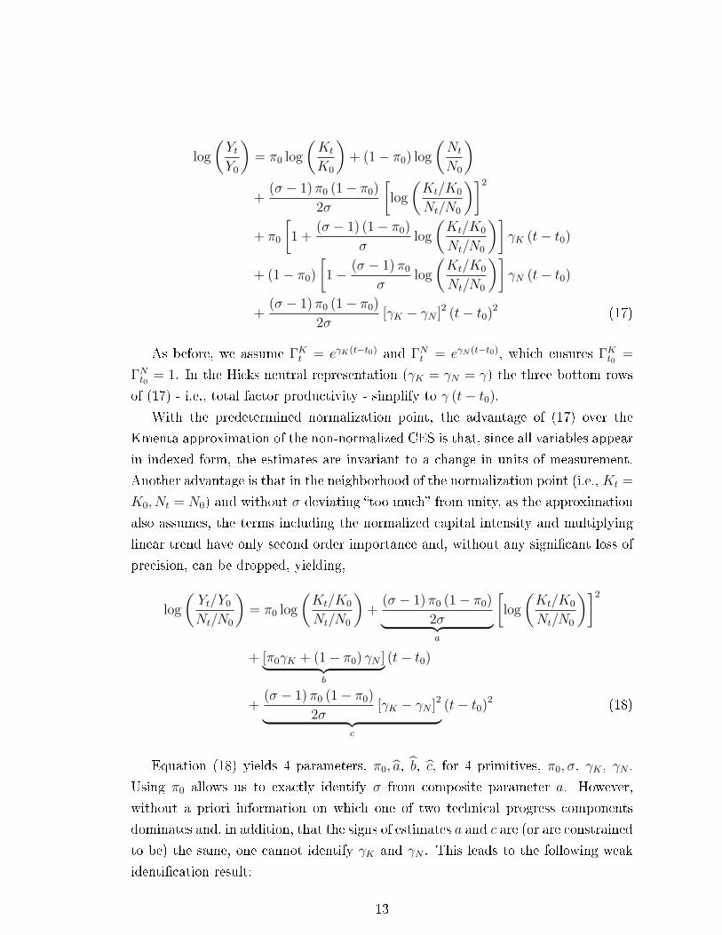
log

(Yt

Y0

)= π0 log

(Kt

K0

)+ (1− π0) log

(Nt

N0

)+

(σ − 1) π0 (1− π0)

2σ

[log

(Kt/K0

Nt/N0

)]2

+ π0

[1 +

(σ − 1) (1− π0)

σlog

(Kt/K0

Nt/N0

)]γK (t− t0)

+ (1− π0)

[1− (σ − 1) π0

σlog

(Kt/K0

Nt/N0

)]γN (t− t0)

+(σ − 1) π0 (1− π0)

2σ[γK − γN ]2 (t− t0)

2 (17)

As before, we assume ΓKt = eγK(t−t0) and ΓN

t = eγN (t−t0), which ensures ΓKt0

=

ΓNt0

= 1. In the Hicks neutral representation (γK = γN = γ) the three bottom rows

of (17) - i.e., total factor productivity - simplify to γ (t− t0).

With the predetermined normalization point, the advantage of (17) over the

Kmenta approximation of the non-normalized CES is that, since all variables appear

in indexed form, the estimates are invariant to a change in units of measurement.

Another advantage is that in the neighborhood of the normalization point (i.e., Kt =

K0, Nt = N0) and without σ deviating �too much� from unity, as the approximation

also assumes, the terms including the normalized capital intensity and multiplying

linear trend have only second order importance and, without any signi�cant loss of

precision, can be dropped, yielding,

log

(Yt/Y0

Nt/N0

)= π0 log

(Kt/K0

Nt/N0

)+

(σ − 1) π0 (1− π0)

2σ︸ ︷︷ ︸a

[log

(Kt/K0

Nt/N0

)]2

+ [π0γK + (1− π0) γN ]︸ ︷︷ ︸b

(t− t0)

+(σ − 1) π0 (1− π0)

2σ[γK − γN ]2︸ ︷︷ ︸

c

(t− t0)2 (18)

Equation (18) yields 4 parameters, π0, a, b, c, for 4 primitives, π0, σ, γK , γN .

Using π0 allows us to exactly identify σ from composite parameter a. However,

without a priori information on which one of two technical progress components

dominates and, in addition, that the signs of estimates a and c are (or are constrained

to be) the same, one cannot identify γK and γN . This leads to the following weak

identi�cation result:

13

for γN > γK we obtain γN = b + π0

√caand γN = b− (1− π0)

√ca

for γN < γK we obtain γN = b− π0

√caand γN = b + (1− π0)

√ca

Given this, although the Kmenta approximation can be used to estimate σ, it

cannot e�ectively identify the direction of the biased technical change.

Finally, note, if σ = 1 then Taylor expanded forms (17) and (18) naturally

reduce to Cobb-Douglas. Furthermore, when σ 6= 1 and technical progress deviates

from Hicks neutrality, factor augmentation introduces additional curvature into the

estimated production function via the quadratic trend both in (17) and (18) and, in

addition, in (17) via the term where capital intensity multiplies the linear trend.

5.2 The System Approach

A still relatively rarely used framework for the estimation of aggregate CES pro-

duction functions is the supply-side system approach (i.e., production function plus

FOC's). Its origin goes back to Marschak and Andrews (1947) in the context of

cross-section analysis, and in the time-series context by Bodkin and Klein (1967).

Since, normalization is implicitly or explicitly employed in all CES production

function, we de�ne the production system as explicitly normalized. To be empirically

applicable, however, the point of normalization must be de�ned in terms of the

underlying data. If the DGP were deterministic, this would be unproblematic: every

sample point would be equally suitable for the point of normalization.15 However, if

the DGP is stochastic this is not so, because the production function does not hold

exactly in any sample point. Therefore, to diminish the size of stochastic component

in the point of normalization we prefer to de�ne the normalization point in terms of

sample averages (geometric averages for growing variables and arithmetic ones for

factor shares).

15It is straightforward to show that the point of normalization can be shifted from point t0 toany point t1 ≥ t0 so that

Yt = Y0

π0

(eγK(t−t0)Kt

K0

)σ−1σ

+ (1− π0)(

eγN (t−t0)Nt

N0

)σ−1σ

σσ−1

= Y1

π1

(eγK(t−t1)Kt

K1

)σ−1σ

+ (1− π1)(

eγN (t−t1)Nt

N1

)σ−1σ

σσ−1

where π1 = π0

[K1/K0Y1/Y0

eγK(t1−t0)]σ−1

σ equalling capital income share at point t1.

14

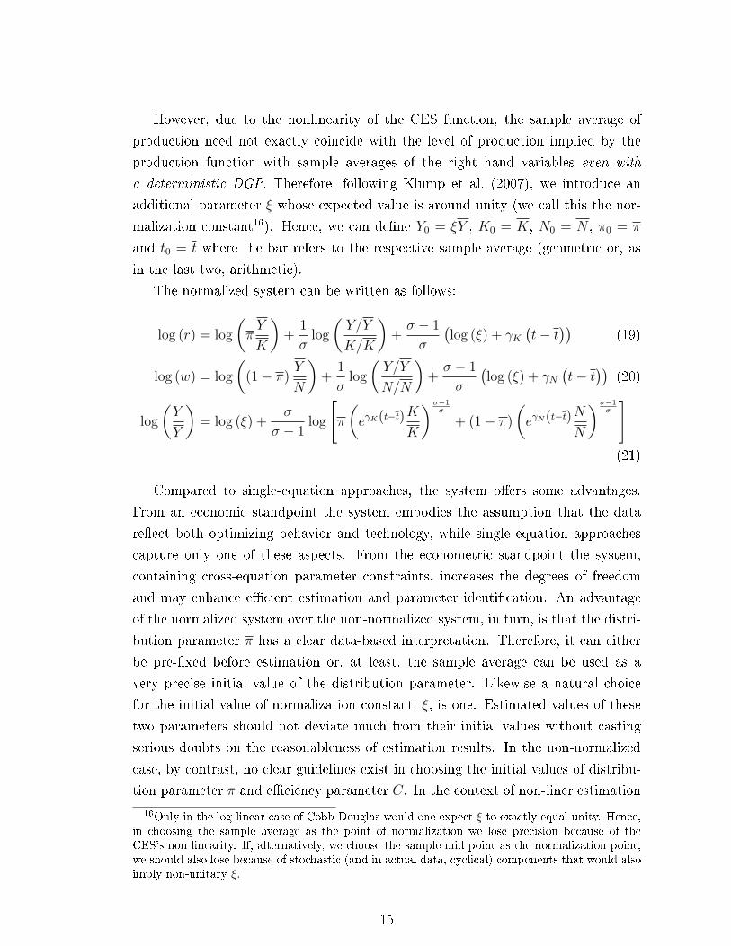
However, due to the nonlinearity of the CES function, the sample average of

production need not exactly coincide with the level of production implied by the

production function with sample averages of the right hand variables even with

a deterministic DGP. Therefore, following Klump et al. (2007), we introduce an

additional parameter ξ whose expected value is around unity (we call this the nor-

malization constant16). Hence, we can de�ne Y0 = ξY , K0 = K, N0 = N , π0 = π

and t0 = t where the bar refers to the respective sample average (geometric or, as

in the last two, arithmetic).

The normalized system can be written as follows:

log (r) = log

(π

Y

K

)+

1

σlog

(Y/Y

K/K

)+

σ − 1

σ

(log (ξ) + γK

(t− t

))(19)

log (w) = log

((1− π)

Y

N

)+

1

σlog

(Y/Y

N/N

)+

σ − 1

σ

(log (ξ) + γN

(t− t

))(20)

log

(Y

Y

)= log (ξ) +

σ

σ − 1log

[π

(eγK(t−t)K

K

)σ−1σ

+ (1− π)

(eγN(t−t)N

N

)σ−1σ

](21)

Compared to single-equation approaches, the system o�ers some advantages.

From an economic standpoint the system embodies the assumption that the data

re�ect both optimizing behavior and technology, while single equation approaches

capture only one of these aspects. From the econometric standpoint the system,

containing cross-equation parameter constraints, increases the degrees of freedom

and may enhance e�cient estimation and parameter identi�cation. An advantage

of the normalized system over the non-normalized system, in turn, is that the distri-

bution parameter π has a clear data-based interpretation. Therefore, it can either

be pre-�xed before estimation or, at least, the sample average can be used as a

very precise initial value of the distribution parameter. Likewise a natural choice

for the initial value of normalization constant, ξ, is one. Estimated values of these

two parameters should not deviate much from their initial values without casting

serious doubts on the reasonableness of estimation results. In the non-normalized

case, by contrast, no clear guidelines exist in choosing the initial values of distribu-

tion parameter π and e�ciency parameter C. In the context of non-liner estimation

16Only in the log-linear case of Cobb-Douglas would one expect ξ to exactly equal unity. Hence,in choosing the sample average as the point of normalization we lose precision because of theCES's non-linearity. If, alternatively, we choose the sample mid-point as the normalization point,we should also lose because of stochastic (and in actual data, cyclical) components that would alsoimply non-unitary ξ.

15

this may imply a signi�cant advantage of the normalized over the non-normalized

system. We examine this in section 7.1.

Finally, the normalized non-linear CES production in isolation is given by equa-

tion (21).

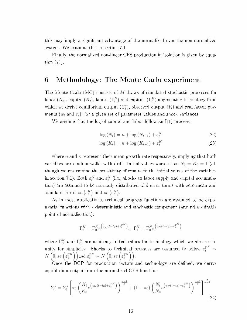
6 Methodology: The Monte Carlo experiment

The Monte Carlo (MC) consists of M draws of simulated stochastic processes for

labor (Nt), capital (Kt), labor- (ΓNt ) and capital- (ΓK

t ) augmenting technology from

which we derive equilibrium output (Y∗t ), observed output (Yt) and real factor pay-

ments (wt and rt), for a given set of parameter values and shock variances.

We assume that the log of capital and labor follow an I(1) process:

log (Nt) = n + log (Nt−1) + εNt (22)

log (Kt) = κ + log (Kt−1) + εKt (23)

where n and κ represent their mean growth rate respectively, implying that both

variables are random walks with drift. Initial values were set as N0 = K0 = 1 (al-

though we re-examine the sensitivity of results to the initial values of the variables

in section 7.1). Both εKt and εN

t (i.e., shocks to labor supply and capital accumula-

tion) are assumed to be normally distributed i.i.d error terms with zero mean and

standard errors se(εK

t

)and se

(εN

t

).

As in most applications, technical progress functions are assumed to be expo-

nential functions with a deterministic and stochastic component (around a suitable

point of normalization):

ΓKt = ΓK

0 e

(γ

K(t−t0)+εΓK

t

), ΓN

t = ΓN0 e

(γN (t−t0)+εΓN

t

)

where ΓK0 and ΓN

0 are arbitrary initial values for technology which we also set to

unity for simplicity. Shocks to technical progress are assumed to follow εΓK

t ∼N

(0, se

(εΓK

t

))and εΓN

t ∼ N(0, se

(εΓN

t

)).

Once the DGP for production factors and technology are de�ned, we derive

equilibrium output from the normalized CES function:

Y ∗t = Y ∗

0

[π0

(Kt

K0

e

(γK(t−t0)+εΓK

t

))σ−1σ

+ (1− π0)

(Nt

N0

e

(γN (t−t0)+εΓN

t

))σ−1σ

] σσ−1

(24)

16

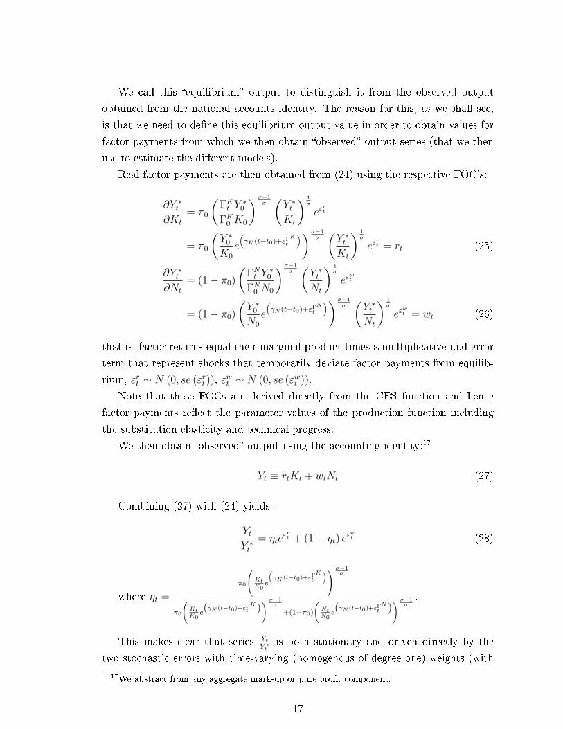
We call this �equilibrium� output to distinguish it from the observed output

obtained from the national accounts identity. The reason for this, as we shall see,

is that we need to de�ne this equilibrium output value in order to obtain values for

factor payments from which we then obtain �observed� output series (that we then

use to estimate the di�erent models).

Real factor payments are then obtained from (24) using the respective FOC's:

∂Y ∗t

∂Kt

= π0

(ΓK

t Y ∗0

ΓK0 K0

)σ−1σ

(Y ∗

t

Kt

) 1σ

eεrt

= π0

(Y ∗

0

K0

e

(γK(t−t0)+εΓK

t

))σ−1σ

(Y ∗

t

Kt

) 1σ

eεrt = rt (25)

∂Y ∗t

∂Nt

= (1− π0)

(ΓN

t Y ∗0

ΓN0 N0

)σ−1σ

(Y ∗

t

Nt

) 1σ

eεwt

= (1− π0)

(Y ∗

0

N0

e

(γN (t−t0)+εΓN

t

))σ−1σ

(Y ∗

t

Nt

) 1σ

eεwt = wt (26)

that is, factor returns equal their marginal product times a multiplicative i.i.d error

term that represent shocks that temporarily deviate factor payments from equilib-

rium, εrt ∼ N (0, se (εr

t )), εwt ∼ N (0, se (εw

t )).

Note that these FOCs are derived directly from the CES function and hence

factor payments re�ect the parameter values of the production function including

the substitution elasticity and technical progress.

We then obtain �observed� output using the accounting identity:17

Yt ≡ rtKt + wtNt (27)

Combining (27) with (24) yields:

Yt

Y ∗t

= ηteεrt + (1− ηt) eεw

t (28)

where ηt =

π0

KtK0

e

(γK (t−t0)+εΓ

Kt

)σ−1

σ

π0

(KtK0

e(γK (t−t0)+εΓK

t ))σ−1

σ

+(1−π0)

(NtN0

e(γN (t−t0)+εΓN

t ))σ−1

σ.

This makes clear that series Yt

Y ∗tis both stationary and driven directly by the

two stochastic errors with time-varying (homogenous of degree one) weights (with

17We abstract from any aggregate mark-up or pure pro�t component.

17

the weights themselves dependent on stochastic technical progress and the factor

indices).

This observed value from (27) is then used to estimate the production function

using the di�erent estimation methods previously described. The reason why we

proceed this way instead of simply adding a stochastic shock to (24) and then

obtaining the FOCs with a shock as in (25) and (26) is that our simulated data has

to be fully consistent: the shares of capital and labor must sum to unity. Had we

proceeded using this alternative way, nothing would have ensured that this condition

is met because our generated data is stochastic (these stochastic shocks may make

factor shares deviate from values consistent with national-accounting identities).

Hence, in our DGP we have shocks to labor supply, capital accumulation, technology,

and factor markets and consistency with national-accounting practice is achieved.

The MC therefore proceeds in the following steps, each of which is repeated M

times:

1. Obtain capital, labor, and technology series using (22)-(23) for sample period

T.

2. Using these series, generate values for equilibrium output and factor payments

using (24)-(26).

3. Obtain an observed output series from (27).

4. Estimate the parameters of the model using the di�erent estimation approaches

explained in section 5 making use of the observed value for output and the

series for capital, labor and factor payments (i.e., the series available to the

econometrician).

Table 2 lists the MC parameters. We set the distribution parameter to 0.4.18

The substitution elasticity ranges from a low 0.2 and 0.5, to a near Cobb-Douglas

(0.9) value and a value exceeding unity, 1.3.

The technical progress parameters are set so as to sum to a reasonable value

of 2% growth per year across the di�erent augmentation forms.19 As in the bulk

of theoretical and empirical studies, we assume broadly constant technical progress

growth rates. To assume time-varying growth rates, mimicking models of �directed�

18We also experimented with values of 0.3 and 0.6, but this made no qualitative di�erence to theresults; accordingly, we kept its value �xed across all experiments to reduce the volume of results.

19We performed experiments where the values did not sum up to 2% per year, with values aslarge as 4%. This did not make any qualitative di�erence to the results of the experiment.

18

technical change (see Kennedy (1964), Samuelson (1965), Zebra (1998), Acemoglu

(2002a), 2003) would require, for instance, agreement on the nature of the economy's

�innovation possibilities frontier� alongside an explicit framework of imperfect com-

petition. Although we address related issues in Section 8.3 below, we leave a detailed

analysis open for future research.

We assume labor supply grows at an average rate of 1.5% per year (roughly the

value for US population growth). We then set the capital stock so that (in equa-

tion 23) the drift parameter κ equals the drift of labor supply growth n plus the

trend growth of labor-augmenting technical progress, γN . This ensures that tech-

nical progress increases per-capita output independently from the nature of factor

augmentation. This formulation allows us to analyze cases in which the evolu-

tion of factor shares is notionally consistent with a balanced growth path (i.e. for

γN = 0.02, γK = 0.00), and cases for which capital and labor shares are (stochasti-

cally) increasing or decreasing, hence covering a wide set of formulations for factor

shares.20

To avoid counter-factual volatility of the simulated data, we paid due attention

to the standard errors of the shocks. We chose a value of 0.1 for the capital and

labor stochastic shocks.21 For the technical-progress parameters we used a value of

0.01 when the technical progress parameter is set to zero, so that the stochastic com-

ponent of technical progress does not dominate. When technical progress exceeds

zero we used a value of 0.05 to capture the likelihood that when technical progress

is present it may also be subject to larger shocks.22

For the case of wage and rental prices we resorted to real data and used the value

of the standard deviation of, respectively, their de-trended and demeaned values in

the US economy over 1950-2000.23 The value for real wages data is 0.05 and 0.3

for capital income, re�ecting the larger volatility of user costs. This di�erential

will have important implications for the relative success of the �rst order conditions

using OLS, as will be discussed later. Accordingly, we also repeated the experiments

where we equate these variances and where we use an instrumental variables (IV)

20We also set κ exogenously to 3% but this, again, did not a�ect the interpretation of results inany signi�cant way.

21This is approximately the standard error of labor and capital equipment around a stochastictrend with drift for US data from 1950 to 2005. If we consider all capital stock, i.e. includinginfrastructures, the standard error is around 0.05. Hence, we reproduced the results using thissmaller variance speci�cation for Kt but this did not a�ect our conclusions.

22Nevertheless, we also replicated the results assuming a zero shock when technical progress iszero and also equal shocks for both components. This, again, did not have any signi�cant e�ecton the results of the experiment.

23We use Bureau of Economic Analysis national accounts data.

19

estimator.

Finally, we consider sample sizes of 25-100 data points (years) with the number

of MC draws set to 5,000.24

7 Results

Of the cases in Table 2, to keep results manageable, we mostly report those relating

to the empirically more relevant T=50 horizon and the combinations γN = 0.015

and γK = 0.005 and γN = 0.005 and γK = 0.015 (Tables 3a and 3b). All other

cases are available on request, although there is no qualitative di�erence in the

interpretation of results (from those shown). We report the median values of the

estimated coe�cients across the 5,000 draws and the 10% and 90% percentiles.25

In terms of the OLS FOC's (the �rst four columns of Tables 3a and 3b) we

generally see poor tracking properties except perhaps at the near-Leontief σ = 0.2

case. The estimated substitution elasticity tends to get trapped around 0.5 as the

true value is increased.26 Estimates of technical progress also appear badly captured.

The exception is the FOC with respect to labor: here the substitution elasticity is

estimated quite precisely (with a slight deterioration of performance for the σ = 1.3

case) as is the growth rate of technical progress.

The reason why one OLS approach dominates can be traced to equations (25)

and (26): the presence of a stochastic component in factor returns that represents

measurement error (or simultaneity bias). In such cases, we know the probability

limit of the estimator tends to its true value depending on the noise-to-signal ratio

(i.e., the variance of the error process V (εt) over that of the independent variable

V (Xt), which in our case is either rt or wt):27

24The non-linear estimations (i.e., direct CES estimation and that of the system) require initial(parameter) conditions. Following Thursby (1980) we set the initial parameter values to thoseobtained from OLS estimates of �rst order conditions. For the technical progress parameters weused the labor and capital FOCs 14 and 13. For σ we used the OLS estimation of the ratiobetween the capital and labor FOC 15. The nature of the non-linear results remains very robustto whichever rule we used.

25We report the median rather than the mean because in some of the nonlinear estimationmethods one cannot rule out abnormal estimation outcomes in some of the draws, which can skewthe results substantially. For maximum transparency, moreover, we ran these MC experimentswithout any distorting, non-replicable user interference: we never imposed any sign or boundsrestriction on any of the parameters. Not with standing, the tables produced relatively few non-standard outcomes.

26Researchers disposed towards high or above-unitary substitution elasticities (e.g., Caballeroand Hammour (1998)) may draw comfort from these results given that many of the OLS systemat-ically under-estimate the elasticity of substitution, with that bias increasing in the true elasticity.

27This argument only applies to the case of two factors of production. The direction of the

20

p lim β =β

1 + V (εt) /V (Xt)

Consider the joint interest-rate/capital marginal-product condition:

∂Y ∗t

∂Kt

= π0

(Y ∗

0

K0

ΓKt

)σ−1σ

(Y ∗

t

Kt

) 1σ

eεrt = rt

For a given π0 and ΓKt , the noise-to-signal ratio is increasing in the substitution

elasticity, limσ→∞

corr(rt, e

εrt

)→ 1, resulting in downward bias. In general, we would

expect the FOC's to perform poorly as σ increases, and especially when above unity.

Indeed, when σ = 0.9 the associated absolute percentage errors (for σ) for K_FOC

(13) and N_FOC (14) are 86% and 4%, respectively; at σ = 1.3 they climb to 167%

and 20%.28

However, in the wage/labor marginal-product condition,

∂Y ∗t

∂Nt

= (1− π0)

(Y ∗

0

N0

ΓNt

)σ−1σ

(Y ∗

t

Nt

) 1σ

eεwt = wt

we have the additional apparent advantage that since output growth exceeds labor

growth, productivity and the real wage are non-stationary. This trending aspect

(compared to a largely stationary capital-output ratio and real interest rate) implies

a generally more favorable noise-to-signal ratio.29

Moreover, since the data (recall Table 2) informs us that se (εrt ) = 0.30 >>

se (εwt ) = 0.05, it is easy to appreciate why this measurement error problem is more

severe in the capital FOC. Setting se (εrt ) = se (εw

t ) eliminated the asymmetry but

is not an option for the econometrician. The only potential solution to this problem

is the use of instrumental variables (IV) estimators. In our case, since we know the

true characteristics of the data, we can make use of good instruments to estimate the

FOCs. By construction, the �rst lag of factor payments will be strongly correlated

with their contemporaneous value as it has been generated by (25) and (26) with

labor and capital following a non-stationary process (22)-(23). However, the shocks

to factor payments in t and t− 1 are un-correlated. This implies that the �rst lags

bias with more than one regressor is generally unknown, and researchers would have to resort tosimulation to understand how measurement error may be a�ecting their estimated parameters.

28We analyzed this argument further obtaining by simulation of what the plim of the estimatedcoe�cient would be given our shock variances and the simulated data for r and w in the MC exper-iment. The results obtained yielded coe�cient values very close to those obtained in estimation,reinforcing the case for this explanation of the OLS bias.

29Although, strictly speaking, this trending aspect will also be a�ected by the dynamics of ΓNt .

21

of log(r) and log(w) can be used as instruments for their contemporaneous values

in (14) and (13) and estimate the equation using Two-Stages Least Squares (2SLS).

The results (available on request) show that the IV estimator resolves the estimation

bias problem, but only as the sample size increases. With T = 30 substantial biases

persist, but for T = 100 the IV estimator correctly identi�es technical progress and

the substitution elasticity even for true values up to 1.3. The obvious problem with

this approach is that, for practical purposes, the econometrician may not have good

instruments and enough observations to eliminate this endogeneity/measurement

error problem.30 For instance, in practise, unlike our experiments, shocks to factor

markets tend to be auto-correlated. If this is the case, one should have to use at

least more complex lag structures for the instruments to achieve identi�cation.31

The Kmenta approximation, as discussed earlier, cannot identify technical progress

parameters and so we only report the results for σ. Results show that this estima-

tion method performs poorly at identifying σ, which is consistently underestimated.

It is noteworthy that as T increases, the Kmenta approximation does a better job at

identifying the true value of the elasticity when it is close to unity.32 This con�rms

our previous argument that the Kmenta approximation deteriorates especially when

it is far from the supporting unitary value.

In terms of the non-linear direct estimate of the production function, its perfor-

mance is close but inferior to the labor FOC in terms of estimating the substitution

elasticity but it has of course the advantage of being able to identify the individual

technical progress parameters.

Results from the normalized system identify it as the superior method.33 Es-

timates of both the elasticity of substitution and technical change are very close

to their true values. This is irrespective of whether we pre-�x the normalization

constant to unity or not.34 The system (as we shall see in section 8.2) performs well

30The FOCs equations were also estimated using Fully Modi�ed OLS methods, but the resultsremained very close to those obtained via OLS.

31We repeated the IV estimation experiment assuming that the shocks to factor markets areautocorrelated with an autocorrelation coe�cient of 0.5. The results showed that using the �rstlag as instrument did not resolve the problem of the OLS bias.

32For instance, for T = 100 and σ = 0.9, the median values obtained for the technical progresscon�gurations shown in Tables 3a and 3b are 0.86 and 0.82 respectively.

33The estimator used for the system is a non-linear Feasible Generalized Least Squares (FGLS)method which accounts for possible cross equation error correlation (much like a SUR model inlinear contexts). The estimator, as implemented in the RATS programming language, performsNLLS on each individual equation and uses the estimated errors to build a variance-covariance(VCV) matrix and then estimates the system by GLS, completing one iteration. The estimatedVCV matrix will be updated with each iteration until the system converges to a predeterminedcriterion.

34The reported results were obtained without pre-�xing ξ.

22

even for relatively small samples. Although our system estimation, unlike single-

equation �rst order equations, were not sensitive with respect to simultaneous bias,

we also checked the performance of the system method under di�erent estimation

techniques by using a 3SLS non-linear estimator (GMM) where we instrumentalized

the variables with their �rst lag. The results did not change, yielding again very

precise estimates of the true parameter values.

7.1 Normalization versus Non-Normalization

A legitimate question to ask is whether normalization makes a di�erence for estima-

tion results with the system.35 As we know, the interpretation of parameters with

non-normalized production functions will in general be di�erent depending on initial

values of the DGP. The normalized system, however, is, by de�nition, invariant to

initial values.

Accordingly, in addition to normalized system (19)-(21) we also estimate the

non-normalized system:

log (r) = log (π) +1

σlog

(Y

K

)+

σ − 1

σ(log (C) + γKt) (29)

log (w) = log (1− π) +1

σlog

(Y

N

)+

σ − 1

σ(log (C) + γN t) (30)

log (Y ) = log (C) +σ

σ − 1log

[π

(eγKtK

)σ−1σ + (1− π)

(eγN tN

)σ−1σ

](31)

As discussed earlier, the major di�erence between the non-normalized system

(29)-(31) and the normalized system (19)-(21) is that, in the former, parameters C

and π are not �deep� but dependent on data values at the normalization point and

the substitution elasticity (recall equations (11) and (12)).

Table 4 presents some consistent sets of (deterministic) initial values for generat-

ing data and the implied ranges of the true values of C and π and for σ ∈ [0.2, 1.3].

In all cases we assumed ΓK0 = ΓN

0 = 1. The �rst row, with initial values of ΓK0

= ΓN0 = Y0 = 1, represents a special case because indexing by the point of nor-

malization equaling one is neutral implying that the true value of C = 1 and

π = π0 = r0 = 0.4 ∀σ. In this special case it does not matter if the same ini-

tial values of parameters are used, whether the system is estimated in normalized

35From the point of view of estimating the �rst order conditions and its relationship to nor-malization, the initial value does not matter, because they can be estimated by linear estimationmethods and the estimated constant takes care of all variation in initial values in generating data.

23

or non-normalized form.

In all other cases, however, this is not so. To illustrate, in these other cases

we have adjusted the initial conditions for output to make them consistent with

an initial (and arguably reasonable) value for r equal to 5%. The sample average

normalization insulates the normalized system from the e�ects of changes in initial

values in generating the data but the true values of composite parameters C and

π vary widely: C ∈ [0.16, 0.49], π ∈ [0.29, 0.99] (interestingly, the actual income

distribution of the data appears unrelated to the true value of π). This illustrates the

di�culty that a practitioner faces when trying to estimate non-normalized system

(29)-(31); actual data scarcely gives any guidelines for appropriate choices for the

initial parameter values of C and π and that results in serious estimation problems.

To examine how uncertainty relating the true values of C and π - and the result-

ing di�culty to de�ne proper initial parameter values for these parameters - a�ect

estimation results, we created data with starting values as presented in the last

two rows of Table 4. Thereafter, we estimated the normalized and non-normalized

systems. In the latter case the initial parameter values for C and π are selected

randomly from their given range. In the �rst (normalized) case, the distribution pa-

rameter π and normalization constant ξ can be pre-set or (as here) freely estimated.

In the estimated case, we have natural priors of the sample average of the capital

income share and unity, respectively.

This comparison is presented in Table 5 where, for brevity, we highlight the

σ = 0.5 and σ = 1.3 cases (the remainder are available on request). One conjecture

rationalizing this result is that to compensate large deviation in initial C from its

true value, the estimation algorithm might minimize this discrepancy via a local

maximum for σ, such that σ → 1,hence σ−1σ→ 0; as can be seen from (29) and (30),

this diminishes the contribution of an incorrect C to overall �t.

This bias increases the more initial conditions depart from their true values.

The fact that both C and π substantially departs from their true, theoretical values,

leads to biased estimates of the substitution elasticity and technical change. There

are, hence, enormous advantages of normalization arising from the pre-�xing of the

distribution parameter and a good initial guess for the normalization constant (which

could further be �xed to unity). Normalization (when combined with a system

approach) appears to be convenient not only for the theoretical interpretation of

deep parameters of the economy, but also for estimation.

24

8 Some Robustness Exercises

Given that results strongly indicate the superiority of the normalized system, we

proceed to investigate some key robustness concerns: namely, (i) residual auto-

correlation, (ii) sample-size power and (iii) alternative forms of technical progress.

8.1 Alternative Shock Processes

We implemented the following auto-correlated shock processes:

(a) AR errors in the technology shocks (εΓK

t and εΓN

t ).

(b) AR errors in the FOC's for N and K (εrt and εw

t ).

(c) (a) and (b) together.

These innovation processes take the form: εit = ρεi

t−1 + ϑt, ϑt ∼ N (0, se (ϑt)),

εi0 = 0 where two ρ values were used: 0.5 and 0.8. The latter represents a very high

degree of persistence for annual data; caution is therefore warranted since this would

imply that our variables are almost not co-integrated (especially for T=25-35). For

brevity, we summarize the outcomes without detailing all the numbers:

1. Overall, when ρ= 0.5 there is no signi�cant bias for any parameter regardless

of the sample size. The results do not change if we consider technical shocks

and FOC shocks as being both auto-correlated (case (c)).

2. When ρ= 0.8 there is only one case in which we have found some bias: for σ=

0.5 and T = 25 and 30 and option (c) implemented. Surprisingly, in the rest

of cases there is only a very small bias in the technical progress coe�cients,

which almost disappears for T = 50 and 100.

8.2 Sample Size Robustness in the System

The Graph shows the performance of the normalized system (for brevity we con-

centrate on the σ = 0.5, γN = 0.015, γK = 0.005 case) when estimated over

T ∈ {25, 100}. The system appears quite robust to sample-size variations. The

main bene�t of larger sample sizes relates to narrower con�dence intervals although

most of that bene�t is achieved by T = 40, 50.

25

8.3 Alternative Forms of Technical Progress

So far, as in the bulk of empirical studies, we assumed linear (constant growth)

technical progress. However, recent contributions as in Acemoglu (2002a, 2003),

McAdam and Willman (2008) have highlighted the role of induced (or directed)

innovations in shaping the dynamics of income distribution. Steady factor incomes

can only be achieved if technical progress is purely labor-augmenting. However,

in the transition towards that steady state, we might expect periods of capital-

augmenting technical progress induced by endogenous changes in the direction of

innovations. Thus, it is not unreasonable to think of non-constant rates of technical

progress. The question then becomes how can this be done in a tractable manner.

Klump et al. (2007) proposed the use of a more �exible speci�cation for Γit based

on the Box-Cox transformation. In the normalized CES function this implies that

Γit = egi(t,t) where gi

(t, t

)= γi

λi

([tt

]λi − 1)

, i = K, N . Curvature parameter λi

determines the shape of the technical progress function. λi = 1 yields the (textbook)

linear speci�cation; λi = 0 a log-linear speci�cation; and λi < 0 a hyperbolic one for

technical progress.

Accordingly, we analyzed the outcome of the Monte Carlo experiment for a

system generated as in Section 5.2 but using the Box-Cox speci�cation for gi (·) asΓi

t = egi(t,t)+εΓit . Together with values for σ ∈ [0.2, 1.3], we used the three following

parameterizations:

(a) γN = 0.015, γK = 0.005, λN = λK = 1.0.

(b) γN = 0.015, γK = 0.030, λN = 0.75, λK = 0.5.

(c) γN = 0.030, γK = 0.015, λN = 1.00, λK = 0.2.

The �rst case corresponds to the linear technological progress speci�cation used

in the previous experiments, which we analyze as a cross-check of earlier results.

The second corresponds to a situation where the growth in both labor- and capital-

augmenting technical progress continuously decelerates and converge asymptotically

to zero (albeit faster for capital-augmenting technical progress). Case (c) implies

that labor-augmenting technical progress is linear with capital-augmenting declining

towards zero somewhat faster than in case (b). In all cases, the standard errors of the

technology shocks were set to 0.01, as in several of these speci�cations technological

progress continuously decelerates and the stochastic part would dominate. This is

also the reason why we choose slightly higher values for γK and γN for cases (b) and

26

(c) than in the previous experiments as, in these cases, low and declining rates of

technical progress are not economically distinguishable from zero.

Table 6 reports the median value of the 5,000 draws for the relevant parameters

using a sample size of T=50. In all the cases, the estimate of σ remains very close to

its true value. The technical progress coe�cients γK and γN are also captured well,

although the bias is slightly larger than that obtained using the linear speci�cation

of previous sections. This is also the case for the curvature parameters λN and λK ,

where the estimated coe�cients are very close to the true ones, but we can observe

upward biases especially for values of σ = 1.3. This, however, is not surprising

given the strong non-linearities introduced by the new terms and, in general, we

see the system remains robust to the introduction of non-constant rates of technical

progress.

9 Conclusions

The elasticity of substitution between capital and labor and the direction of techni-

cal change are pivotal parameters in many areas of economics. The received wisdom,

in both theoretical and empirical literatures, suggests that their joint identi�cation

is infeasible. If so, this would render indeterminate a wide range of economic in-

quiries. However, given the vigor of recent debates on biased technical change (Ace-

moglu (2002a)); the shape of the local/global production function (Acemoglu (2003),

Jones (2005)); the importance of normalization (La Grandville (1989), Klump and

de La Grandville (2000)); and renewed interest in the estimated CES function itself

(Klump et al. (2007)), disentangling these e�ects remains a key, unresolved matter.

We re-examined these issues using a comprehensive Monte Carlo exercise. We

con�rm that using many conventional approaches, identi�cation problems can be

substantial. In terms of the success of the FOCs, results depend on the relative

shock processes of the measurement errors (implying that the labor FOC equation

tends to work better). Although we derived some new identi�cation results for the

normalized (factor-augmenting) Kmenta approximation, identi�cation of the sub-

stitution elasticity remains poor and that of technical change bleak. Also, direct

estimation of the non-linear CES function remains highly problematic. However in

contrast to the conventional approaches, our results suggested that the system ap-

proach of jointly estimating the FOCs and the production function worked extremely

well and appeared robust to error mis-speci�cation, sample-size variation and alter-

native forms of technical progress. Normalization adds considerably to these gains:

27

it allows the pre-setting of the capital income share; it provides a clear correspon-

dence between theoretical and empirical production parameters; allows us ex-post

validation of estimated parameters; and facilitates the setting of initial parameter

conditions.

Accordingly, our results o�er relief to the chronic identi�cation concerns raised

in the literature. Thus, we hope to have contributed towards better estimation

practices, a better understanding of previous empirical �ndings, as well as to a more

wide-spread appreciation of the properties of factor-augmenting (normalized) CES

functions.

Acknowledgements

We thank Daron Acemoglu, Ricardo Caballero, Robert Chirinko, William Greene

(discussant), Rainer Klump, Marianne Saam, Katsuyuki Shibayama, Robert Solow,

Tony Thirwall, Anders Warne, and seminar audiences at MIT, Kent, Goethe, GRE-

QAM, the 2008 EEA, the ECB and Pablo de Olavide for helpful comments and

discussions. McAdam is also visiting professor at Surrey and further thanks the

MIT economics department for its hospitality where he was a visiting scholar dur-

ing earlier stages of this work. The opinions expressed are not necessarily those of

the ECB.

28

References

Acemoglu, D. (2002a). Directed technical change. Review of Economic Studies,69:781�809.

Acemoglu, D. (2002b). Technical Change, Inequality and the Labor Market. Journalof Economic Literature, 40(1):7�72.

Acemoglu, D. (2003). Labor- and capital-augmenting technical change. Journal ofthe European Economic Association, 1:1�37.

Acemoglu, D. (2008). Introduction to Modern Economic Growth. MIT Press, forth-coming.

Antràs, P. (2004). Is the US Aggregate Production Function Cobb-Douglas? NewEstimates of the Elasticity of Substitution. Contributions to Macroeconomics,4(Article 4):1.

Arrow, K. J., Chenery, H., Minhas, B. S., and Solow, R. M. (1961). Capital-laborsubstitution and economic e�ciency. Review of Economics and Statistics, 43:225�250.

Bairam, E. I. (1991). Functional form and the new production function: somecomments and a new ves. Applied Economics, 23(7):1247�49.

Basu, S. and Fernald, J. (1997). Returns to Scale in U.S. Manufacturing: Estimatesand Implications. Journal of Political Economy, 105(2):249�283.

Berndt, E. R. (1976). Reconciling alternative estimates of the elasticity of substitu-tion. Review of Economics and Statistics, 58:59�68.

Berndt, E. R. (1991). The Practice of Econometrics. Addison Wesley.

Berthold, N., Fehn, R., and Thode, E. (2002). Falling labour share and rising un-employment: Long-run consequences of institutional shocks? German EconomicReview, 3:431�459.

Blanchard, O. J. (1997). The Medium Run. Brookings Papers on Economic Activity,2:89�158.

Bodkin, R. G. and Klein, L. R. (1967). Nonlinear estimation of aggregate productionfunctions. Review of Economics and Statistics, 49:28�44.

Caballero, R. J. (1994). Small sample bias and adjustment costs. Review of Eco-nomics and Statistics, 85:153�65.

Caballero, R. J. and Hammour, M. (1998). Jobless growth: Appropriablity, fac-tor substitution and unemployment. Carnegie-Rochester Conference Proceedings,48:51�94.

Chirinko, R. S. (2008). Sigma: The Long and Short of It. Journal of Macroeco-nomics, 30(2):671�686.

David, P. A. and van de Klundert, T. (1965). Biased e�ciency growth and capital-labor substitution in the US, 1899-1960. American Economic Review, 55:357�394.

29

Diamond, P., Fadden, D. M., and Rodriguez, M. (1978). Measurement of the elas-ticity of substitution and bias of technical change. In Fuss, M. and Fadden, D. M.,editors, Production economics, Vol. 2, pages 125�147. Amsterdam and North Hol-land.

Dickinson, H. (1955). A Note on Dynamic Economies. Review of Economic Studies,22(3):169�179.

Du�y, J. and Papageorgiou, C. (2000). A cross-country empirical investigation ofthe aggregate production function speci�cation. Journal of Economic Growth,5:86�120.

Genç, M. and Bairam, E. I. (1998). The Box-Cox Transformation as a VES Produc-tion Function. in E. I. Bairam, Production and Cost Functions, Ashgate Press.

Hardy, G. H., Littlewood, J. E., and Polya, G. (1934). Inequalities. CambridgeUniversity Press, 2nd ed. 1952.

Jones, C. I. (2005). The shape of production functions and the direction of technicalchange. Quarterly Journal of Economics, 120(2):517�549.

Jones, R. (1965). The structure of simple general equilibrium models. Journal ofPolitical Economy, 73(6):557�572.

Kamien, M. I. and Schwartz, N. L. (1968). Optimal Induced technical change.Econometrica, 36:1�17.

Kennedy, C. (1964). Induced bias in innovation and the theory of distribution.Economic Journal, 74:541�547.

Klump, R. and de La Grandville, O. (2000). Economic growth and the elasticity ofsubstitution: two theorems and some suggestions. American Economic Review,90:282�291.

Klump, R., McAdam, P., and Willman, A. (2007). Factor Substitution and FactorAugmenting Technical Progress in the US. Review of Economics and Statistics,89(1):183�92.

Klump, R. and Preissler, H. (2000). CES production functions and economic growth.Scandinavian Journal of Economics, 102:41�56.

Kmenta, J. (1967). On Estimation of the CES Production Function. InternationalEconomic Review, 8:180�189.

Kumar, T. K. and Gapinski, J. H. (1974). Nonlinear estimation of the CES Produc-tion Function Parameters: A Monte Carlo. Review of Economics and Statistics,56(4):563�567.

La Grandville, O. d. (1989). In quest of the Slutzky diamond. American EconomicReview, 79:468�481.

La Grandville, O. d. (2008). Economic Growth: A Uni�ed Approach. CambridgeUniversity Press.

La Grandville, O. d. and Solow, R. M. (2006). A conjecture on general means.Journal of Inequalities in Pure and Applied Mathematics, 7(3).

30

La Grandville, O. d. and Solow, R. M. (2008). Capital-labour substitution andeconomic growth. In La Grandville, O. d., editor, Economic Growth: A Uni�edApproach. Cambridge University Press, forthcoming.

Maddala, G. S. and Kadane, J. B. (1966). Some notes on the estimation of theconstant elasticity of substitution function. Review of Economics and Statistics,48(3):340�344.

Mankiw, N. G. (1995). The growth of nations. Brookings Papers on EconomicActivity, 1:275�310.

Marquetti, A. A. (2003). Analyzing historical and regional patterns of technicalchange from a classical-marxian perspective. Journal of Economic Behavior andOrganization, 52:191�200.

Marschak, J. and Andrews, W. (1947). Random simultaneous equations and thetheory of production. Econometrica, 12:143�53.

McAdam, P. and Willman, A. (2008). Medium Run Redux. Working Paper No.915, European Central Bank.

Pitchford, J. (1960). Growth and the elasticity of substitution. Economic Record,36:491�504.

Rowthorn, R. (1999). Unemployment, wage bargaining and capital-labour substitu-tion. Cambridge Journal of Economics, 23:413�425.

Samuelson, P. A. (1965). A Theory of Induced Innovations along Kennedy-WeisackerLines. Review of Economics and Statistics, 47(4):344�356.

Solow, R. M. (1956). A contribution to the theory of economic growth. QuarterlyJournal of Economics, 70:65�94.

ten Cate, A. (1992). Data Scaling With Highly Non-Linear Regression. Computa-tional Statistics, 7:59�65.

Thursby, J. (1980). Alternative CES estimation techniques. Review of Economicsand Statistics, 62(2):259�299.

Willman, A. (2002). Euro area production function and potential output: a supplyside system approach. Working Paper No. 153, European Central Bank.

Yuhn, K.-h. (1991). Economic Growth, Technical Change Biases, and the Elasticityof Substitution: A Test of the De La Grandville Hypothesis. Review of Economicsand Statistics, 73(2):340�346.

31

Table 1. Empirical Studies of Aggregate Elasticity of Substitution and Technological Change in the US 

Estimated Annual Rate Of Efficiency Change 

Study  Sample Assumption on Technological 

Change 

Estimated Elasticity of Substitution 

σ  

Hicks Neutral: 

N Kγ γ=  

Labor‐ Augmenting: 

Nγ  

Capital‐ Augmenting: 

Kγ  

Arrow et al. (1961)  1909‐1949  Hicks‐Neutral 0.57  1.8  ‐  ‐ 

Kendrick and Sato (1963)  1919‐1960  Hicks‐Neutral 0.58  2.1  ‐  ‐ 

Brown and De Cani (1963) 

1890‐1918 

1919‐1937 

1938‐1958 

1890‐1958 

Factor Augmenting 

0.35 

0.08 

0.11 

0.44 

Labor saving ( N Kγ γ− = 0.48) 

Labor saving ( N Kγ γ− = 0.62) 

Labor saving ( N Kγ γ− = 0.36) ? 

David and van de Klundert (1965)  1899‐1960 

Factor Augmenting  0.32  ‐  2.2  1.5 

Bodkin and Klein (1967)  1909‐1949  Hicks‐neutral  0.5‐0.7  1.4‐1.5     

Wilkinson (1968)  1899‐1953 Factor 

Augmenting  0.5  Labor saving ( N Kγ γ− = 0.51) 

Sato (1970)  1909‐1960 Factor 

Augmenting  0.5–0.7  ‐  2.0  1.0 

Panik (1976)  1929‐1966 Factor 

Augmenting  0.76  Labor saving  ( N Kγ γ− = 0.27) 

Berndt (1976)  1929‐1968  Hicks‐neutral  0.96‐1.25  ?  ‐  ‐ 

Kalt (1978)  1929‐1967  Factor Augmenting 

0.76  ‐  2.2  0.01 

Hicks‐neutral  0.94‐1.02  1.14  ‐  ‐ Antràs (2004)  1948‐1998  Factor‐

augmenting 0.80  Labor saving ( N Kγ γ− = 3.15) 

Klump, McAdam and Willman 

(2007) 1953‐1998 

Factor‐augmenting  0.56  ‐  1.5  0.4 

32

33

Table 2. Monte Carlo Parameter Values. 

Parameter 

Values 

π: D

istribution pa

rameter 

0.4 

σ: Sub

stitu

tion elasticity 

0.2, 0.5, 0.9, 1.3 

Kγ: G

rowth Rate of cap

ital‐a

ugmentin

g technical p

rogress* 

0.00, 0.005, 0.01, 0.015, 0.02 

Nγ: G

rowth Rate of labo

r‐au

gmentin

g technical p

rogress* 

0.02, 0.015, 0.01, 0.005, 0.00 

η: L

abor Force growth ra

te 

0.015 

κ: C

apita

l Stock growth ra

te 

Nγη+

 

)(

),(

K tN t

sese

εε

: Stand

ard Error in the La

bor a

nd Cap

ital D

GP shock 

0.10 

)(

K

tse

Γ ε: Stand

ard Error in Cap

ital‐A

ugmentin

g Te

chnical P

rogress shock 

0.01 fo

r 0

=Kγ

; 0.05 for 

0≠

Kγ 

)(

N

tse

Γ ε: Stand

ard Error in La

bor‐Aug

mentin

g Te

chnical P

rogress shock 

0.01 fo

r 0

=Nγ

; 0.05 for 

0≠

Nγ 

)(

w tse

ε: Stand

ard Error o

f Real W

age shock 

0.05 

)(

r tse

ε: Stand

ard Error o

f Real Interest R

ate shock 

0.30 

() t

seϑ

: Stand

ard Error o

f AR(1) error sho

ck 

0.10 

T: Sam

ple Size (a

nnua

l) 25 – 100 

M: M

onte Carlo Draws 

5,000 

Note: *, 

02.0=

+N

Kγ

γ 

33

Table 2. Monte Carlo Parameter Values. 

Parameter 

Values 

π: D

istribution pa

rameter 

0.4 

σ: Sub

stitu

tion elasticity 

0.2, 0.5, 0.9, 1.3 

Kγ: G

rowth Rate of cap

ital‐a

ugmentin

g technical p

rogress* 

0.00, 0.005, 0.01, 0.015, 0.02 

Nγ: G

rowth Rate of labo

r‐au

gmentin

g technical p

rogress* 

0.02, 0.015, 0.01, 0.005, 0.00 

η: L

abor Force growth ra

te 

0.015 

κ: C

apita

l Stock growth ra

te 

Nγη+

 

)(

),(

K tN t

sese

εε

: Stand

ard Error in the La

bor a

nd Cap

ital D

GP shock 

0.10 

)(

K

tse

Γ ε: Stand

ard Error in Cap

ital‐A

ugmentin

g Te

chnical P

rogress shock 

0.01 fo

r 0

=Kγ

; 0.05 for 

0≠

Kγ 

)(

N

tse

Γ ε: Stand

ard Error in La

bor‐Aug

mentin

g Te

chnical P

rogress shock 

0.01 fo

r 0

=Nγ

; 0.05 for 

0≠

Nγ 

)(

w tse

ε: Stand

ard Error o

f Real W

age shock 

0.05 

)(

r tse

ε: Stand

ard Error o

f Real Interest R

ate shock 

0.30 

() t

seϑ

: Stand

ard Error o

f AR(1) error sho

ck 

0.10 

T: Sam

ple Size (a

nnua

l) 25 – 100 

M: M

onte Carlo Draws 

5,000 

Note: *, 

02.0=

+N

Kγ

γ 

                                                                                   Table 3a. 

0.01

5γ

0.00

5,γ

50,

TN

K=

==

 Single Equation FOCs 

 K_FOC 

N_FOC 

Factor Prices 

Factor Sha

res 

Kmenta 

Non‐Linear CES 

System 

2.0=

σ 

σ

0.22

4 [0

.185

: 0

.602

] 0.

211

[0.1

07 :

0.45

2]

0.17

0 [0

.145

: 0

.188

] 0.

164

[0.1

36 :

0.18

4]

0.18

0 [-

0.36

62 :

0.72

6]

0.26

1 [0

.078

: 1.

000]

0.

232

[0.2

04 :

0.28

7]

Kγ

0.00

4 [-

0.01

1 : 0

.008

] —

——

—0.

004

[-0.

016

: 0.0

30]

0.00

4 [0

.000

: 0.

007]

Nγ

—

0.01

4 [0

.009

: 0.

018]

—

—

—0.

014

[-0.

001

: 0.0

24]

0.01

5 [0

.010

: 0

.019

]

ˆˆ

KN

γγ

−

—

—

-0.0

11

[-0.

017

:- 0.

006]

-0

.011

[-

0.01

8 :-

0.00

5]

—

-0.0

11

[0.0

37 :

0.03

4]

-0.0

10

[-0.

015

: -0.

007]

ζ

—

[0

.996

: 1.

098]

1.

026

1.02

8 [1

.007

: 1.

077]

5.0=

σ

σ

0.43

6 [0

.357

: 0.

539]

0.

537

[0.3

69 :

0.71

8]

0.29

1 [0

.195

: 0.

382]

0.

204

[0.1

13 :

0.30

6]

0.34

70

[-0.

603

: 1.1

73]

0.42

2 [0

.109

: 1.

110]

0.

541

[0.5

02 :

0.60

1]

Kγ

0.00

3 [-

0.00

5 : 0

.006

] —

——

—0.

003

[-

0.01

9 : 0

.028

] 0.

005

[0.0

02 :

0.01

]

Nγ

—

0.01

4 [0

.005

: 0.

020]

—

—

—0.

015

[-

0.00

2 : 0

.025

] 0.

015

[0.0

11 :

0.0

19]

ˆˆ

KN

γγ

−

—

—

-0.0

13

[-0.

029

: 0.0

03]

-0.0

13

[-0.

034

: 0.0

06]

—

-0.0

12

[-0.

043

: 0.0

30]

-0.0

09

[-0.

016

: -0.

002]

ζ

—

1.

015

[0.9

81 :

1.05

5]

1.00

8 [0

.999

: 1.

034]

9.0=

σ

σ

0.48

1 [0

.426

: 0.

551]

0.

870

[0.6

24 :

1.10

8]

0.27

7 [0

.153

: 0.

456]

0.

041

[-0.

074

: 0.1

47]

0.41

96

[-1.

21 :

1.98

] 0.

612

[0.1

07 :

2E5]

0.

873

[0.8

04 :

0.95

1]

Kγ

0.00

2 [-

0.01

4 : 0

.018

] —

——

—0.

003

[-0.

038

: 0.0

78]

0.00

5 [-

0.00

5 : 0

.025

]

Nγ

—

0.01

7 [-

0.00

8 : 0

.043

] —

—

—0.

015

[-0.

022

: 0.0

44]

0.01

6 [-

0.00

1 : 0

.031

]

ˆˆ

KN

γγ

−

—

—

-0.0

15

[-0.

042

: 0.0

13]

-0.0

15

[-0.

043

: 0.0

14]

—

-0.0

12

[-0.

079

: 0.1

13]

-0.0

11

[-0.

046

: 0.0

25]

ζ

—

1.

002

[0.9

63 :

1.03

6]

0.99

7 [0

.995

: 1.

005]

3.1=

σ

σ

0.48

3 [0

.417

: 0.

561]

1.

049

[0.7

26 :

1.34

5]

0.22

8 [0

.098

: 0.

419]

-0

.095

[-

0.30

6 : 0

.024

] 0.

386

[-1.

487

: 2.0

6]

1.01

8 [-

1E5

: 3E6

] 1.

237

[0.9

30 :

1.35

5]

Kγ

0.00

2 [-

0.01

8 : 0

.022

] —

——

—0.

005

[-0.

032

: 0.1

07]

0.00

6 [-

0.00

6: 0

.068

]

Nγ

—

0.01

6 [-

0.01

5 : 0

.049

] —

—

—0.

014

[-0.

055

: 0.0

39]

0.01

4 [-

0.02

8 : 0

.066

]

ˆˆ

KN

γγ

−

—

—

-0.0

15

[-0.

045

: 0.0

15]

-0.0

14

[-0.

042

: 0.0

13]

—

-0.0

09

[-0.

069

: 0.1

67]

-0.0

08

[-0.

134

: 0.0

95]

ζ

—

[0

.941

: 1.

021]

0.

976

0.99

0 [0

.975

: 1.

003]

34

                                                                                   Table 3a. 

0.01

5γ

0.00

5,γ

50,

TN

K=

==

 Single Equation FOCs 

 K_FOC 

N_FOC 

Factor Prices 

Factor Sha

res 

Kmenta 

Non‐Linear CES 

System 

2.0=

σ 

σ

0.22

4 [0

.185

: 0

.602

] 0.

211

[0.1

07 :

0.45

2]

0.17

0 [0

.145

: 0

.188

] 0.

164

[0.1

36 :

0.18

4]

0.18

0 [-

0.36

62 :

0.72

6]

0.26

1 [0

.078

: 1.

000]

0.

232

[0.2

04 :

0.28

7]

Kγ

0.00

4 [-

0.01

1 : 0

.008

] —

——

—0.

004

[-0.

016

: 0.0

30]

0.00

4 [0

.000

: 0.

007]

Nγ

—

0.01

4 [0

.009

: 0.

018]

—

—

—0.

014

[-0.

001

: 0.0

24]

0.01

5 [0

.010

: 0

.019

]

ˆˆ

KN

γγ

−

—

—

-0.0

11

[-0.

017

:- 0.

006]

-0

.011

[-

0.01

8 :-

0.00

5]

—

-0.0

11

[0.0

37 :

0.03

4]

-0.0

10

[-0.

015

: -0.

007]

ζ

—

[0

.996

: 1.

098]

1.

026

1.02

8 [1

.007

: 1.

077]

5.0=

σ

σ

0.43

6 [0

.357

: 0.

539]

0.

537

[0.3

69 :

0.71

8]

0.29

1 [0

.195

: 0.

382]

0.

204

[0.1

13 :

0.30

6]

0.34

70

[-0.

603

: 1.1

73]

0.42

2 [0

.109

: 1.

110]

0.

541

[0.5

02 :

0.60

1]

Kγ

0.00

3 [-

0.00

5 : 0

.006

] —

——

—0.

003

[-

0.01

9 : 0

.028

] 0.

005

[0.0

02 :

0.01

]

Nγ

—

0.01

4 [0

.005

: 0.

020]

—

—

—0.

015

[-

0.00

2 : 0

.025

] 0.

015

[0.0

11 :

0.0

19]

ˆˆ

KN

γγ

−

—

—

-0.0

13

[-0.

029

: 0.0

03]

-0.0

13

[-0.

034

: 0.0

06]

—

-0.0

12

[-0.

043

: 0.0

30]

-0.0

09

[-0.

016

: -0.

002]

ζ

—

1.

015

[0.9

81 :

1.05

5]

1.00

8 [0

.999

: 1.

034]

9.0=

σ

σ

0.48

1 [0

.426

: 0.

551]

0.

870

[0.6

24 :

1.10

8]

0.27

7 [0

.153

: 0.

456]

0.

041

[-0.

074

: 0.1

47]

0.41

96

[-1.

21 :

1.98

] 0.

612

[0.1

07 :

2E5]

0.

873

[0.8

04 :

0.95

1]

Kγ

0.00

2 [-

0.01

4 : 0

.018

] —

——

—0.

003

[-0.

038

: 0.0

78]

0.00

5 [-

0.00

5 : 0

.025

]

Nγ

—

0.01

7 [-

0.00

8 : 0

.043

] —

—

—0.

015

[-0.

022

: 0.0

44]

0.01

6 [-

0.00

1 : 0

.031

]

ˆˆ

KN

γγ

−

—

—

-0.0

15

[-0.

042

: 0.0

13]

-0.0

15

[-0.

043

: 0.0

14]

—

-0.0

12

[-0.

079

: 0.1

13]

-0.0

11

[-0.

046

: 0.0

25]

ζ

—

1.

002

[0.9

63 :

1.03

6]

0.99

7 [0

.995

: 1.

005]

3.1=

σ

σ

0.48

3 [0

.417

: 0.

561]

1.

049

[0.7

26 :

1.34

5]

0.22

8 [0

.098

: 0.

419]

-0

.095

[-

0.30

6 : 0

.024

] 0.

386

[-1.

487

: 2.0

6]

1.01

8 [-

1E5

: 3E6

] 1.

237

[0.9

30 :

1.35

5]

Kγ

0.00

2 [-

0.01

8 : 0

.022

] —

——

—0.

005

[-0.

032

: 0.1

07]

0.00

6 [-

0.00

6: 0

.068

]

Nγ

—

0.01

6 [-

0.01

5 : 0

.049

] —

—

—0.

014

[-0.

055

: 0.0

39]

0.01

4 [-

0.02

8 : 0

.066

]

ˆˆ

KN

γγ

−

—

—

-0.0

15

[-0.

045

: 0.0

15]

-0.0

14

[-0.

042

: 0.0

13]

—

-0.0

09

[-0.

069

: 0.1

67]

-0.0

08

[-0.

134

: 0.0

95]

ζ

—

[0

.941

: 1.

021]

0.

976

0.99

0 [0

.975

: 1.

003]

34

                                                                                   Table 3a. 

0.01

5γ

0.00

5,γ

50,

TN

K=

==

 Single Equation FOCs 

 K_FOC 

N_FOC 

Factor Prices 

Factor Sha

res 

Kmenta 

Non‐Linear CES 

System 

2.0=

σ 

σ

0.22

4 [0

.185

: 0

.602

] 0.

211

[0.1

07 :

0.45

2]

0.17

0 [0

.145

: 0

.188

] 0.

164

[0.1

36 :

0.18

4]

0.18

0 [-

0.36

62 :

0.72

6]

0.26

1 [0

.078

: 1.

000]

0.

232

[0.2

04 :

0.28

7]

Kγ

0.00

4 [-

0.01

1 : 0

.008

] —

——

—0.

004

[-0.

016

: 0.0

30]

0.00

4 [0

.000

: 0.

007]

Nγ

—

0.01

4 [0

.009

: 0.

018]

—

—

—0.

014

[-0.

001

: 0.0

24]

0.01

5 [0

.010

: 0

.019

]

ˆˆ

KN

γγ

−

—

—

-0.0

11

[-0.

017

:- 0.

006]

-0

.011

[-

0.01

8 :-

0.00

5]

—

-0.0

11

[0.0

37 :

0.03

4]

-0.0

10

[-0.

015

: -0.

007]

ζ

—

[0

.996

: 1.

098]

1.

026

1.02

8 [1

.007

: 1.

077]

5.0=

σ

σ

0.43

6 [0

.357

: 0.

539]

0.

537

[0.3

69 :

0.71

8]

0.29

1 [0

.195

: 0.

382]

0.

204

[0.1

13 :

0.30

6]

0.34

70

[-0.

603

: 1.1

73]

0.42

2 [0

.109

: 1.

110]

0.

541

[0.5

02 :

0.60

1]

Kγ

0.00

3 [-

0.00

5 : 0

.006

] —

——

—0.

003

[-

0.01

9 : 0

.028

] 0.

005

[0.0

02 :

0.01

]

Nγ

—

0.01

4 [0

.005

: 0.

020]

—

—

—0.

015

[-

0.00

2 : 0

.025

] 0.

015

[0.0

11 :

0.0

19]

ˆˆ

KN

γγ

−

—

—

-0.0

13

[-0.

029

: 0.0

03]

-0.0

13

[-0.

034

: 0.0

06]

—

-0.0

12

[-0.

043

: 0.0

30]

-0.0

09

[-0.

016

: -0.

002]

ζ

—

1.

015

[0.9

81 :

1.05

5]

1.00

8 [0

.999

: 1.

034]

9.0=

σ

σ

0.48

1 [0

.426

: 0.

551]

0.

870

[0.6

24 :

1.10

8]

0.27

7 [0

.153

: 0.

456]

0.

041

[-0.

074

: 0.1

47]

0.41

96

[-1.

21 :

1.98

] 0.

612

[0.1

07 :

2E5]

0.

873

[0.8

04 :

0.95

1]

Kγ

0.00

2 [-

0.01

4 : 0

.018

] —

——

—0.

003

[-0.

038

: 0.0

78]

0.00

5 [-

0.00

5 : 0

.025

]

Nγ

—

0.01

7 [-

0.00

8 : 0

.043

] —

—

—0.

015

[-0.

022

: 0.0

44]

0.01

6 [-

0.00

1 : 0

.031

]

ˆˆ

KN

γγ

−

—

—

-0.0

15

[-0.

042

: 0.0

13]

-0.0

15

[-0.

043

: 0.0

14]

—

-0.0

12

[-0.

079

: 0.1

13]

-0.0

11

[-0.

046

: 0.0

25]

ζ

—

1.

002

[0.9

63 :

1.03

6]

0.99

7 [0

.995

: 1.

005]

3.1=

σ

σ

0.48

3 [0

.417

: 0.

561]

1.

049

[0.7

26 :

1.34

5]

0.22

8 [0

.098

: 0.

419]

-0

.095

[-

0.30

6 : 0

.024

] 0.

386

[-1.

487

: 2.0

6]

1.01

8 [-

1E5

: 3E6

] 1.

237

[0.9

30 :

1.35

5]

Kγ

0.00

2 [-

0.01

8 : 0

.022

] —

——

—0.

005

[-0.

032

: 0.1

07]

0.00

6 [-

0.00

6: 0

.068

]

Nγ

—

0.01

6 [-

0.01

5 : 0

.049

] —

—

—0.

014

[-0.

055

: 0.0

39]

0.01

4 [-

0.02

8 : 0

.066

]

ˆˆ

KN

γγ

−

—

—

-0.0

15

[-0.

045

: 0.0

15]

-0.0

14

[-0.

042

: 0.0

13]

—

-0.0

09

[-0.

069

: 0.1

67]

-0.0

08

[-0.

134

: 0.0

95]

ζ

—

[0

.941

: 1.

021]

0.

976

0.99

0 [0

.975

: 1.

003]

34

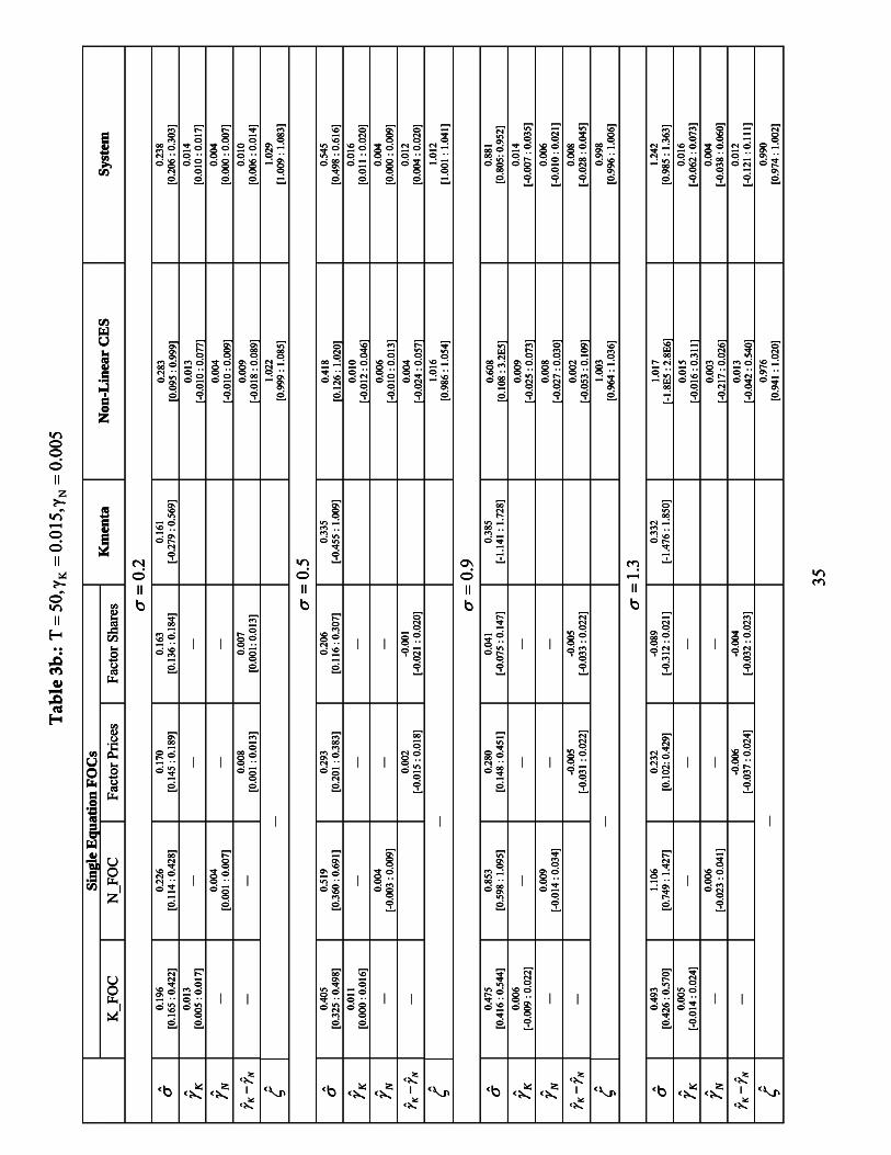
Table 3b.: 

0.00

5γ

0.01

5,γ

50,

TN

K=

==

 

Sing

le E

quat

ion

FOC

s

K_F

OC

N

_FO

C

Fact

or P

rices

Fa

ctor

Sha

res

Km

enta

Non

-Lin

ear

CE

SSy

stem

2.0=

σ

σ

0.19

6 [0

.165

: 0.

422]

0.

226

[0.1

14 :

0.42

8]

0.17

0 [0

.145

: 0.

189]

0.

163

[0.1

36 :

0.18

4]

0.16

1 [-

0.27

9 : 0

.569

] 0.

283

[0.0

95 :

0.99

9]

0.23

8 [0

.206

: 0.

303]

Kγ

0.01

3 [0

.005

: 0.

017]

—

——

0.01

3 [-

0.01

0 : 0

.077

] 0.

014

[0.0

10 :

0.01

7]

Nγ

—

0.00

4 [0

.001

: 0.

007]

—

—

0.00

4 [-

0.01

0 : 0

.009

] 0.

004

[0.0

00 :

0.00

7]

ˆˆ

KN

γγ

−

—

—

0.00

8 [0

.001

: 0.

013]

0.

007

[0.0

01: 0

.013

]

0.00

9 [-

0.01

8 : 0

.089

] 0.

010

[0.0

06 :

0.01

4]

ζ

—

[0

.999

: 1.

085]

1.

022

1.02

9 [1

.009

: 1.

083]

5.0=

σ

σ

0.40

5 [0

.325

: 0.

498]

0.

519

[0.3

60 :

0.69

1]

0.29

3 [0

.201

: 0.

383]

0.

206

[0.1

16 :

0.30

7]

0.33

5 [-

0.45

5 : 1

.009

] 0.

418

[0.1

26 :

1.02

0]

0.54

5 [0

.498

: 0.

616]

Kγ

0.01

1 [0

.000

: 0.

016]

—

——

0.01

0 [-

0.01

2 : 0

.046

] 0.

016

[0.0

11 :

0.02

0]

Nγ

—

0.00

4 [-

0.00

3 : 0

.009

] —

—

0.00

6 [-

0.01

0 : 0

.013

] 0.

004

[0.0

00 :

0.00

9]

ˆˆ

KN

γγ

−

—

0.

002

[-0.

015

: 0.0

18]

-0.0

01

[-0.

021

: 0.0

20]

0.

004

[-0.

024

: 0.0

57]

0.01

2 [0

.004

: 0.

020]

ζ

—

1.

016

[0.9

86 :

1.05

4]

1.01

2 [1

.001

: 1.

041]

9.0=

σ

σ

0.47

5 [0

.416

: 0.

544]

0.

853

[0.5

98 :

1.09

5]

0.28

0 [0

.148

: 0.

451]

0.

041

[-0.

075

: 0.1

47]

0.38

5 [-

1.14

1 : 1

.728

] 0.

608

[0.1

08 :

3.2E

5]

0.88

1 [0

.805

: 0.9

52]

Kγ

0.00

6 [-

0.00

9 : 0

.022

] —

——

0.00

9 [-

0.02

5 : 0

.073

] 0.

014

[-0.

007

: 0.0

35]

Nγ

—

0.00

9 [-

0.01

4 : 0

.034

] —

—

0.00

8 [-

0.02

7 : 0

.030

] 0.

006

[-0.

010

: 0.0

21]

ˆˆ

KN

γγ

−

—

-0

.005

[-

0.03

1 : 0

.022

] -0

.005

[-

0.03

3 : 0

.022

]

0.00

2 [-

0.05

3 : 0

.109

] 0.

008

[-0.

028

: 0.0

45]

ζ

—

1.

003

[0.9

64 :

1.03

6]

0.99

8 [0

.996

: 1.

006]

3.1=

σ

σ

0.49

3 [0

.426

: 0.

570]

1.

106

[0.7

49 :

1.42

7]

0.23

2 [0

.102

: 0.4

29]

-0.0

89

[-0.

312

: 0.0

21]

0.33

2 [-

1.47

6 : 1

.850

] 1.

017

[-1.

8E5

: 2.8

E6]

1.24

2 [0

.985

: 1.

363]

Kγ

0.00

5 [-

0.01

4 : 0

.024

] —

——

0.01

5 [-

0.01

6 : 0

.311

] 0.

016

[-0.

062

: 0.0

73]

Nγ

—

0.00

6 [-

0.02

3 : 0

.041

] —

—

0.00

3 [-

0.21

7 : 0

.026

] 0.

004

[-0.

038

: 0.0

60]

ˆˆ

KN

γγ

−

—

-0

.006

[-

0.03

7 : 0

.024

] -0

.004

[-

0.03

2 : 0

.023

]

0.01

3 [-

0.04

2 : 0

.540

] 0.

012

[-0.

121

: 0.1

11]

ζ

—

0.

976

[0.9

41 :

1.02

0]

0.99

0 [0

.974

: 1.

002]

35

Table 3b.: 

0.00

5γ

0.01

5,γ

50,

TN

K=

==

 

Sing

le E

quat

ion

FOC

s

K_F

OC

N

_FO

C

Fact

or P

rices

Fa

ctor

Sha

res

Km

enta

Non

-Lin

ear

CE

SSy

stem

2.0=

σ

σ

0.19

6 [0

.165

: 0.

422]

0.

226

[0.1

14 :

0.42

8]

0.17

0 [0

.145

: 0.

189]

0.

163

[0.1

36 :

0.18

4]

0.16

1 [-

0.27

9 : 0

.569

] 0.

283

[0.0

95 :

0.99

9]

0.23

8 [0

.206

: 0.

303]

Kγ

0.01

3 [0

.005

: 0.

017]

—

——

0.01

3 [-

0.01

0 : 0

.077

] 0.

014

[0.0

10 :

0.01

7]

Nγ

—

0.00

4 [0

.001

: 0.

007]

—

—

0.00

4 [-

0.01

0 : 0

.009

] 0.

004

[0.0

00 :

0.00

7]

ˆˆ

KN

γγ

−

—

—

0.00

8 [0

.001

: 0.

013]

0.

007

[0.0

01: 0

.013

]

0.00

9 [-

0.01

8 : 0

.089

] 0.

010

[0.0

06 :

0.01

4]

ζ

—

[0

.999

: 1.

085]

1.

022

1.02

9 [1

.009

: 1.

083]

5.0=

σ

σ

0.40

5 [0

.325

: 0.

498]

0.

519

[0.3

60 :

0.69

1]

0.29

3 [0

.201

: 0.

383]

0.

206

[0.1

16 :

0.30

7]

0.33

5 [-

0.45

5 : 1

.009

] 0.

418

[0.1

26 :

1.02

0]

0.54

5 [0

.498

: 0.

616]

Kγ

0.01

1 [0

.000

: 0.

016]

—

——

0.01

0 [-

0.01

2 : 0

.046

] 0.

016

[0.0

11 :

0.02

0]

Nγ

—

0.00

4 [-

0.00

3 : 0

.009

] —

—

0.00

6 [-

0.01

0 : 0

.013

] 0.

004

[0.0

00 :

0.00

9]

ˆˆ

KN

γγ

−

—

0.

002

[-0.

015

: 0.0

18]

-0.0

01

[-0.

021

: 0.0

20]

0.

004

[-0.

024

: 0.0

57]

0.01

2 [0

.004

: 0.

020]

ζ

—

1.

016

[0.9

86 :

1.05

4]

1.01

2 [1

.001

: 1.

041]

9.0=

σ

σ

0.47

5 [0

.416

: 0.

544]

0.

853

[0.5

98 :

1.09

5]

0.28

0 [0

.148

: 0.

451]

0.

041

[-0.

075

: 0.1

47]

0.38

5 [-

1.14

1 : 1

.728

] 0.

608

[0.1

08 :

3.2E

5]

0.88

1 [0

.805

: 0.9

52]

Kγ

0.00

6 [-

0.00

9 : 0

.022

] —

——

0.00

9 [-

0.02

5 : 0

.073

] 0.

014

[-0.

007

: 0.0

35]

Nγ

—

0.00

9 [-

0.01

4 : 0

.034

] —

—

0.00

8 [-

0.02

7 : 0

.030

] 0.

006

[-0.

010

: 0.0

21]

ˆˆ

KN

γγ

−

—

-0

.005

[-

0.03

1 : 0

.022

] -0

.005

[-

0.03

3 : 0

.022

]

0.00

2 [-

0.05

3 : 0

.109

] 0.

008

[-0.

028

: 0.0

45]

ζ

—

1.

003

[0.9

64 :

1.03

6]

0.99

8 [0

.996

: 1.

006]

3.1=

σ

σ

0.49

3 [0

.426

: 0.

570]

1.

106

[0.7

49 :

1.42

7]

0.23

2 [0

.102

: 0.4

29]

-0.0

89

[-0.

312

: 0.0

21]

0.33

2 [-

1.47

6 : 1

.850

] 1.

017

[-1.

8E5

: 2.8

E6]

1.24

2 [0

.985

: 1.

363]

Kγ

0.00

5 [-

0.01

4 : 0

.024

] —

——

0.01

5 [-

0.01

6 : 0

.311

] 0.

016

[-0.

062

: 0.0

73]

Nγ

—

0.00

6 [-

0.02

3 : 0

.041

] —

—

0.00

3 [-

0.21

7 : 0

.026

] 0.

004

[-0.

038

: 0.0

60]

ˆˆ

KN

γγ

−

—

-0

.006

[-

0.03

7 : 0

.024

] -0

.004

[-

0.03

2 : 0

.023

]

0.01

3 [-

0.04

2 : 0

.540

] 0.

012

[-0.

121

: 0.1

11]

ζ

—

0.

976

[0.9

41 :

1.02

0]

0.99

0 [0

.974

: 1.

002]

35

Table 3b.: 

0.00

5γ

0.01

5,γ

50,

TN

K=

==

 

Sing

le E

quat

ion

FOC

s

K_F

OC

N

_FO

C

Fact

or P

rices

Fa

ctor

Sha

res

Km

enta

Non

-Lin

ear

CE

SSy

stem

2.0=

σ

σ

0.19

6 [0

.165

: 0.

422]

0.

226

[0.1

14 :

0.42

8]

0.17

0 [0

.145

: 0.

189]

0.

163

[0.1

36 :

0.18

4]

0.16

1 [-

0.27

9 : 0

.569

] 0.

283

[0.0

95 :

0.99

9]

0.23

8 [0

.206

: 0.

303]

Kγ

0.01

3 [0

.005

: 0.

017]

—

——

0.01

3 [-

0.01

0 : 0

.077

] 0.

014

[0.0

10 :

0.01

7]

Nγ

—

0.00

4 [0

.001

: 0.

007]

—

—

0.00

4 [-

0.01

0 : 0

.009

] 0.

004

[0.0

00 :

0.00

7]

ˆˆ

KN

γγ

−

—

—

0.00

8 [0

.001

: 0.

013]

0.

007

[0.0

01: 0

.013

]

0.00

9 [-

0.01

8 : 0

.089

] 0.

010

[0.0

06 :

0.01

4]

ζ

—

[0

.999

: 1.

085]

1.

022

1.02

9 [1

.009

: 1.

083]

5.0=

σ

σ

0.40

5 [0

.325

: 0.

498]

0.

519

[0.3

60 :

0.69

1]

0.29

3 [0

.201

: 0.

383]

0.

206

[0.1

16 :

0.30

7]

0.33

5 [-

0.45

5 : 1

.009

] 0.

418

[0.1

26 :

1.02

0]

0.54

5 [0

.498

: 0.

616]

Kγ

0.01

1 [0

.000

: 0.

016]

—

——

0.01

0 [-

0.01

2 : 0

.046

] 0.

016

[0.0

11 :

0.02

0]

Nγ

—

0.00

4 [-

0.00

3 : 0

.009

] —

—

0.00

6 [-

0.01

0 : 0

.013

] 0.

004

[0.0

00 :

0.00

9]

ˆˆ

KN

γγ

−

—

0.

002

[-0.

015

: 0.0

18]

-0.0

01

[-0.

021

: 0.0

20]

0.

004

[-0.

024

: 0.0

57]

0.01

2 [0

.004

: 0.

020]

ζ

—

1.

016

[0.9

86 :

1.05

4]

1.01

2 [1

.001

: 1.

041]

9.0=

σ

σ

0.47

5 [0

.416

: 0.

544]

0.

853

[0.5

98 :

1.09

5]

0.28

0 [0

.148

: 0.

451]

0.

041

[-0.

075

: 0.1

47]

0.38

5 [-

1.14

1 : 1

.728

] 0.

608

[0.1

08 :

3.2E

5]

0.88

1 [0

.805

: 0.9

52]

Kγ

0.00

6 [-

0.00

9 : 0

.022

] —

——

0.00

9 [-

0.02

5 : 0

.073

] 0.

014

[-0.

007

: 0.0

35]

Nγ

—

0.00

9 [-

0.01

4 : 0

.034

] —

—

0.00

8 [-

0.02

7 : 0

.030

] 0.

006

[-0.

010

: 0.0

21]

ˆˆ

KN

γγ

−

—

-0

.005

[-

0.03

1 : 0

.022

] -0

.005

[-

0.03

3 : 0

.022

]

0.00

2 [-

0.05

3 : 0

.109

] 0.

008

[-0.

028

: 0.0

45]

ζ

—

1.

003

[0.9

64 :

1.03

6]

0.99

8 [0

.996

: 1.

006]

3.1=

σ

σ

0.49

3 [0

.426

: 0.

570]

1.

106

[0.7

49 :

1.42

7]

0.23

2 [0

.102

: 0.4

29]

-0.0

89

[-0.

312

: 0.0

21]

0.33

2 [-

1.47

6 : 1

.850

] 1.

017

[-1.

8E5

: 2.8

E6]

1.24

2 [0

.985

: 1.

363]

Kγ

0.00

5 [-

0.01

4 : 0

.024

] —

——

0.01

5 [-

0.01

6 : 0

.311

] 0.

016

[-0.

062

: 0.0

73]

Nγ

—

0.00

6 [-

0.02

3 : 0

.041

] —

—

0.00

3 [-

0.21

7 : 0

.026

] 0.

004

[-0.

038

: 0.0

60]

ˆˆ

KN

γγ

−

—

-0

.006

[-

0.03

7 : 0

.024

] -0

.004

[-

0.03

2 : 0

.023

]

0.01

3 [-

0.04

2 : 0

.540

] 0.

012

[-0.

121

: 0.1

11]

ζ

—

0.

976

[0.9

41 :

1.02

0]

0.99

0 [0

.974

: 1.

002]

35

Table 3b.: 

0.00

5γ

0.01

5,γ

50,

TN

K=

==

 

Sing

le E

quat

ion

FOC

s

K_F

OC

N

_FO

C

Fact

or P

rices

Fa

ctor

Sha

res

Km

enta

Non

-Lin

ear

CE

SSy

stem

2.0=

σ

σ

0.19

6 [0

.165

: 0.

422]

0.

226

[0.1

14 :

0.42

8]

0.17

0 [0

.145

: 0.

189]

0.

163

[0.1

36 :

0.18

4]

0.16

1 [-

0.27

9 : 0

.569

] 0.

283

[0.0

95 :

0.99

9]

0.23

8 [0

.206

: 0.

303]

Kγ

0.01

3 [0

.005

: 0.

017]

—

——

0.01

3 [-

0.01

0 : 0

.077

] 0.

014

[0.0

10 :

0.01

7]

Nγ

—

0.00

4 [0

.001

: 0.

007]

—

—

0.00

4 [-

0.01

0 : 0

.009

] 0.

004

[0.0

00 :

0.00

7]

ˆˆ

KN

γγ

−

—

—

0.00

8 [0

.001

: 0.

013]

0.

007

[0.0

01: 0

.013

]

0.00

9 [-

0.01

8 : 0

.089

] 0.

010

[0.0

06 :

0.01

4]

ζ

—

[0

.999

: 1.

085]

1.

022

1.02

9 [1

.009

: 1.

083]

5.0=

σ

σ

0.40

5 [0

.325

: 0.

498]

0.

519

[0.3

60 :

0.69

1]

0.29

3 [0

.201

: 0.

383]

0.

206

[0.1

16 :

0.30

7]

0.33

5 [-

0.45

5 : 1

.009

] 0.

418

[0.1

26 :

1.02

0]

0.54

5 [0

.498

: 0.

616]

Kγ

0.01

1 [0

.000

: 0.

016]

—

——

0.01

0 [-

0.01

2 : 0

.046

] 0.

016

[0.0

11 :

0.02

0]

Nγ

—

0.00

4 [-

0.00

3 : 0

.009

] —

—

0.00

6 [-

0.01

0 : 0

.013

] 0.

004

[0.0

00 :

0.00

9]

ˆˆ

KN

γγ

−

—

0.

002

[-0.

015

: 0.0

18]

-0.0

01

[-0.

021

: 0.0

20]

0.

004

[-0.

024

: 0.0

57]

0.01

2 [0

.004

: 0.

020]

ζ

—

1.

016

[0.9

86 :

1.05

4]

1.01

2 [1

.001

: 1.

041]

9.0=

σ

σ

0.47

5 [0

.416

: 0.

544]

0.

853

[0.5

98 :

1.09

5]

0.28

0 [0

.148

: 0.

451]

0.

041

[-0.

075

: 0.1

47]

0.38

5 [-

1.14

1 : 1

.728

] 0.

608

[0.1

08 :

3.2E

5]

0.88

1 [0

.805

: 0.9

52]

Kγ

0.00

6 [-

0.00

9 : 0

.022

] —

——

0.00

9 [-

0.02

5 : 0

.073

] 0.

014

[-0.

007

: 0.0

35]

Nγ

—

0.00

9 [-

0.01

4 : 0

.034

] —

—

0.00

8 [-

0.02

7 : 0

.030

] 0.

006

[-0.

010

: 0.0

21]

ˆˆ

KN

γγ

−

—

-0

.005

[-

0.03

1 : 0

.022

] -0

.005

[-

0.03

3 : 0

.022

]

0.00

2 [-

0.05

3 : 0

.109

] 0.

008

[-0.

028

: 0.0

45]

ζ

—

1.

003

[0.9

64 :

1.03

6]

0.99

8 [0

.996

: 1.

006]

3.1=

σ

σ

0.49

3 [0

.426

: 0.

570]

1.

106

[0.7

49 :

1.42

7]

0.23

2 [0

.102

: 0.4

29]

-0.0

89

[-0.

312

: 0.0

21]

0.33

2 [-

1.47

6 : 1

.850

] 1.

017

[-1.

8E5

: 2.8

E6]

1.24

2 [0

.985

: 1.

363]

Kγ

0.00

5 [-

0.01

4 : 0

.024

] —

——

0.01

5 [-

0.01

6 : 0

.311

] 0.

016

[-0.

062

: 0.0

73]

Nγ

—

0.00

6 [-

0.02

3 : 0

.041

] —

—

0.00

3 [-

0.21

7 : 0

.026

] 0.

004

[-0.

038

: 0.0

60]

ˆˆ

KN

γγ

−

—

-0

.006

[-

0.03

7 : 0

.024

] -0

.004

[-

0.03

2 : 0

.023

]

0.01

3 [-

0.04

2 : 0

.540

] 0.

012

[-0.

121

: 0.1

11]

ζ

—

0.

976

[0.9

41 :

1.02

0]

0.99

0 [0

.974

: 1.

002]

35

             Table 4. Consistent Normalization Values 

C 

π 

0N 

0π 

0r 

0K 

000

00

Kr

YY

π=

=∗

 (

)0

00

01

NY

wπ

−=

 Max 

Min 

Max 

Min 

1 0.4 

0.4 

1 1 

0.6 

1 0.4 

1 0.4 

0.05 

5 0.625 

0.375 

0.352 

0.157 

0.998 

0.315 

1 0.4 

0.05 

8 1 

0.6 

0.488 

0.157 

0.999 

0.292 

Notes: C and  π in th

e fin

al tw

o columns are calculated according to 4.4a an

d 4.4b for 

[] 3.1,2.0

∈σ

; outside of the “spe

cial 

case” no

te the following pa

rtial de

rivativ

es sho

wing ho

w ceteris paribus cha

nges in initial value

s chan

ge these last tw

o 

parameters:  , 

0,

,0,

;0,0

,,

,0

00

00

00

><

<>

wK

NN

wK

YC

CC

CC

ππ

ππ σ

σ.

36

             Table 4. Consistent Normalization Values 

C 

π 

0N 

0π 

0r 

0K 

000

00

Kr

YY

π=

=∗

 (

)0

00

01

NY

wπ

−=

 Max 

Min 

Max 

Min 

1 0.4 

0.4 

1 1 

0.6 

1 0.4 

1 0.4 

0.05 

5 0.625 

0.375 

0.352 

0.157 

0.998 

0.315 

1 0.4 

0.05 

8 1 

0.6 

0.488 

0.157 

0.999 

0.292 

Notes: C and  π in th

e fin

al tw

o columns are calculated according to 4.4a an

d 4.4b for 

[] 3.1,2.0

∈σ

; outside of the “spe

cial 

case” no

te the following pa

rtial de

rivativ

es sho

wing ho

w ceteris paribus cha

nges in initial value

s chan

ge these last tw

o 

parameters:  , 

0,

,0,

;0,0

,,

,0

00

00

00

><

<>

wK

NN

wK

YC

CC

CC

ππ

ππ σ

σ.

36

             Table 4. Consistent Normalization Values 

C 

π 

0N 

0π 

0r 

0K 

000

00

Kr

YY

π=

=∗

 (

)0

00

01

NY

wπ

−=

 Max 

Min 

Max 

Min 

1 0.4 

0.4 

1 1 

0.6 

1 0.4 

1 0.4 

0.05 

5 0.625 

0.375 

0.352 

0.157 

0.998 

0.315 

1 0.4 

0.05 

8 1 

0.6 

0.488 

0.157 

0.999 

0.292 

Notes: C and  π in th

e fin

al tw

o columns are calculated according to 4.4a an

d 4.4b for 

[] 3.1,2.0

∈σ

; outside of the “spe

cial 

case” no

te the following pa

rtial de

rivativ

es sho

wing ho

w ceteris paribus cha

nges in initial value

s chan

ge these last tw

o 

parameters:  , 

0,

,0,

;0,0

,,

,0

00

00

00

><

<>

wK

NN

wK

YC

CC

CC

ππ

ππ σ

σ.

36

             Table 4. Consistent Normalization Values 

C 

π 

0N 

0π 

0r 

0K 

000

00

Kr

YY

π=

=∗

 (

)0

00

01

NY

wπ

−=

 Max 

Min 

Max 

Min 

1 0.4 

0.4 

1 1 

0.6 

1 0.4 

1 0.4 

0.05 

5 0.625 

0.375 

0.352 

0.157 

0.998 

0.315 

1 0.4 

0.05 

8 1 

0.6 

0.488 

0.157 

0.999 

0.292 

Notes: C and  π in th

e fin

al tw

o columns are calculated according to 4.4a an

d 4.4b for 

[] 3.1,2.0

∈σ

; outside of the “spe

cial 

case” no

te the following pa

rtial de

rivativ

es sho

wing ho

w ceteris paribus cha

nges in initial value

s chan

ge these last tw

o 

parameters:  , 

0,

,0,

;0,0

,,

,0

00

00

00

><

<>

wK

NN

wK

YC

CC

CC

ππ

ππ σ

σ.

36

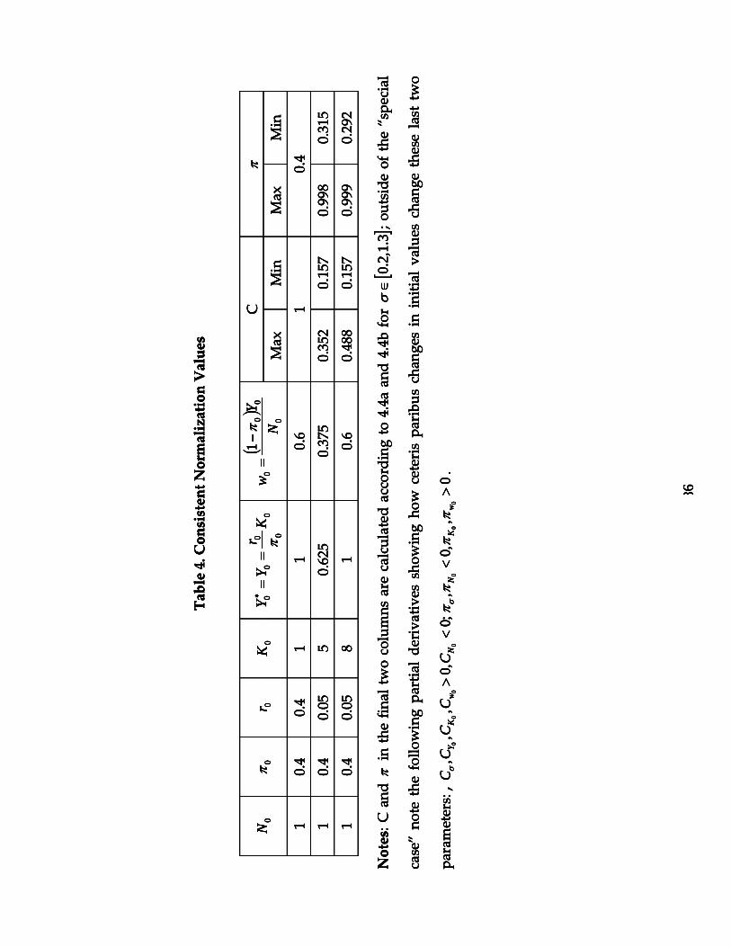
             Table 4. Consistent Normalization Values 

C 

π 

0N 

0π 

0r 

0K 

000

00

Kr

YY

π=

=∗

 (

)0

00

01

NY

wπ

−=

 Max 

Min 

Max 

Min 

1 0.4 

0.4 

1 1 

0.6 

1 0.4 

1 0.4 

0.05 

5 0.625 

0.375 

0.352 

0.157 

0.998 

0.315 

1 0.4 

0.05 

8 1 

0.6 

0.488 

0.157 

0.999 

0.292 

Notes: C and  π in th

e fin

al tw

o columns are calculated according to 4.4a an

d 4.4b for 

[] 3.1,2.0

∈σ

; outside of the “spe

cial 

case” no

te the following pa

rtial de

rivativ

es sho

wing ho

w ceteris paribus cha

nges in initial value

s chan

ge these last tw

o 

parameters:  , 

0,

,0,

;0,0

,,

,0

00

00

00

><

<>

wK

NN

wK

YC

CC

CC

ππ

ππ σ

σ.

36

Table 5. Normalized .vs. Non‐Normalized System Results. 

 Case: 

015

.0,

005

.0,

50=

==

NK

Tγ

γ 

 

Normalized 

 

Non‐Normalized

Normalized 

Non‐Normalized

Normalized 

Non‐Normalized

Normalized 

Non‐Normalized 

625

.0,5

,10

00

==

=Y

KN

1,8

,10

00

==

=Y

KN

 

5.0=

σ

3.1=

σ

5.0=

σ

3.1=

σ

σ

0.54

1

0.

808

1.23

71.

090

0.54

10.

870

1.23

7 1.

039

Kγ

0.00

5

-0

.005

0.00

6-0

.032

0.00

5-0

.012

0.

006

-0.0

42

Nγ

0.01

5

0.

030

0.01

40.

036

0.01

50.

028

0.01

4 -0

.044

NK

γγ

ˆˆ

−

-0.0

09

-0.0

42-0

.008

-0.0

68-0

.009

-0.0

41

-0.0

08

-0.0

87

π

Pref

ixed

to

Sam

ple

aver

age

—

Pref

ixed

to

Sam

ple

aver

age

—

Pref

ixed

to

Sam

ple

aver

age

—

Pref

ixed

to

Sam

ple

aver

age

—

π

–

0.

421

—0.

412

–0.

422

—

0.41

3

ξ

1.00

8

–

0.99

0–

1.00

8–

0.99

0 –

C

–

0.

343

–0.

298

–0.

493

– 0.

324

Not

e: M

edia

n va

lues

repo

rted.

37

Table 5. Normalized .vs. Non‐Normalized System Results. 

 Case: 

015

.0,

005

.0,

50=

==

NK

Tγ

γ 

 

Normalized 

 

Non‐Normalized

Normalized 

Non‐Normalized

Normalized 

Non‐Normalized

Normalized 

Non‐Normalized 

625

.0,5

,10

00

==

=Y

KN

1,8

,10

00

==

=Y

KN

 

5.0=

σ

3.1=

σ

5.0=

σ

3.1=

σ

σ

0.54

1

0.

808

1.23

71.

090

0.54

10.

870

1.23

7 1.

039

Kγ

0.00

5

-0

.005

0.00

6-0

.032

0.00

5-0

.012

0.

006

-0.0

42

Nγ

0.01

5

0.

030

0.01

40.

036

0.01

50.

028

0.01

4 -0

.044

NK

γγ

ˆˆ

−

-0.0

09

-0.0

42-0

.008

-0.0

68-0

.009

-0.0

41

-0.0

08

-0.0

87

π

Pref

ixed

to

Sam

ple

aver

age

—

Pref

ixed

to

Sam

ple

aver

age

—

Pref

ixed

to

Sam

ple

aver

age

—

Pref

ixed

to

Sam

ple

aver

age

—

π

–

0.

421

—0.

412

–0.

422

—

0.41

3

ξ

1.00

8

–

0.99

0–

1.00

8–

0.99

0 –

C

–

0.

343

–0.

298

–0.

493

– 0.

324

Not

e: M

edia

n va

lues

repo

rted.

37

Table 5. Normalized .vs. Non‐Normalized System Results. 

 Case: 

015

.0,

005

.0,

50=

==

NK

Tγ

γ 

 

Normalized 

 

Non‐Normalized

Normalized 

Non‐Normalized

Normalized 

Non‐Normalized

Normalized 

Non‐Normalized 

625

.0,5

,10

00

==

=Y

KN

1,8

,10

00

==

=Y

KN

 

5.0=

σ

3.1=

σ

5.0=

σ

3.1=

σ

σ

0.54

1

0.

808

1.23

71.

090

0.54

10.

870

1.23

7 1.

039

Kγ

0.00

5

-0

.005

0.00

6-0

.032

0.00

5-0

.012

0.

006

-0.0

42

Nγ

0.01

5

0.

030

0.01

40.

036

0.01

50.

028

0.01

4 -0

.044

NK

γγ

ˆˆ

−

-0.0

09

-0.0

42-0

.008

-0.0

68-0

.009

-0.0

41

-0.0

08

-0.0

87

π

Pref

ixed

to

Sam

ple

aver

age

—

Pref

ixed

to

Sam

ple

aver

age

—

Pref

ixed

to

Sam

ple

aver

age

—

Pref

ixed

to

Sam

ple

aver

age

—

π

–

0.

421

—0.

412

–0.

422

—

0.41

3

ξ

1.00

8

–

0.99

0–

1.00

8–

0.99

0 –

C

–

0.

343

–0.

298

–0.

493

– 0.

324

Not

e: M

edia

n va

lues

repo

rted.

37

Table 5. Normalized .vs. Non‐Normalized System Results. 

 Case: 

015

.0,

005

.0,

50=

==

NK

Tγ

γ 

 

Normalized 

 

Non‐Normalized

Normalized 

Non‐Normalized

Normalized 

Non‐Normalized

Normalized 

Non‐Normalized 

625

.0,5

,10

00

==

=Y

KN

1,8

,10

00

==

=Y

KN

 

5.0=

σ

3.1=

σ

5.0=

σ

3.1=

σ

σ

0.54

1

0.

808

1.23

71.

090

0.54

10.

870

1.23

7 1.

039

Kγ

0.00

5

-0

.005

0.00

6-0

.032

0.00

5-0

.012

0.

006

-0.0

42

Nγ

0.01

5

0.

030

0.01

40.

036

0.01

50.

028

0.01

4 -0

.044

NK

γγ

ˆˆ

−

-0.0

09

-0.0

42-0

.008

-0.0

68-0

.009

-0.0

41

-0.0

08

-0.0

87

π

Pref

ixed

to

Sam

ple

aver

age

—

Pref

ixed

to

Sam

ple

aver

age

—

Pref

ixed

to

Sam

ple

aver

age

—

Pref

ixed

to

Sam

ple

aver

age

—

π

–

0.

421

—0.

412

–0.

422

—

0.41

3

ξ

1.00

8

–

0.99

0–

1.00

8–

0.99

0 –

C

–

0.

343

–0.

298

–0.

493

– 0.

324

Not

e: M

edia

n va

lues

repo

rted.

37

Table 5. Normalized .vs. Non‐Normalized System Results. 

 Case: 

015

.0,

005

.0,

50=

==

NK

Tγ

γ 

 

Normalized 

 

Non‐Normalized

Normalized 

Non‐Normalized

Normalized 

Non‐Normalized

Normalized 

Non‐Normalized 

625

.0,5

,10

00

==

=Y

KN

1,8

,10

00

==

=Y

KN

 

5.0=

σ

3.1=

σ

5.0=

σ

3.1=

σ

σ

0.54

1

0.

808

1.23

71.

090

0.54

10.

870

1.23

7 1.

039

Kγ

0.00

5

-0

.005

0.00

6-0

.032

0.00

5-0

.012

0.

006

-0.0

42

Nγ

0.01

5

0.

030

0.01

40.

036

0.01

50.

028

0.01

4 -0

.044

NK

γγ

ˆˆ

−

-0.0

09

-0.0

42-0

.008

-0.0

68-0

.009

-0.0

41

-0.0

08

-0.0

87

π

Pref

ixed

to

Sam

ple

aver

age

—

Pref

ixed

to

Sam

ple

aver

age

—

Pref

ixed

to

Sam

ple

aver

age

—

Pref

ixed

to

Sam

ple

aver

age

—

π

–

0.

421

—0.

412

–0.

422

—

0.41

3

ξ

1.00

8

–

0.99

0–

1.00

8–

0.99

0 –

C

–

0.

343

–0.

298

–0.

493

– 0.

324

Not

e: M

edia

n va

lues

repo

rted.

37

Table 5. Normalized .vs. Non‐Normalized System Results. 

 Case: 

015

.0,

005

.0,

50=

==

NK

Tγ

γ 

 

Normalized 

 

Non‐Normalized

Normalized 

Non‐Normalized

Normalized 

Non‐Normalized

Normalized 

Non‐Normalized 

625

.0,5

,10

00

==

=Y

KN

1,8

,10

00

==

=Y

KN

 

5.0=

σ

3.1=

σ

5.0=

σ

3.1=

σ

σ

0.54

1

0.

808

1.23

71.

090

0.54

10.

870

1.23

7 1.

039

Kγ

0.00

5

-0

.005

0.00

6-0

.032

0.00

5-0

.012

0.

006

-0.0

42

Nγ

0.01

5

0.

030

0.01

40.

036

0.01

50.

028

0.01

4 -0

.044

NK

γγ

ˆˆ

−

-0.0

09

-0.0

42-0

.008

-0.0

68-0

.009

-0.0

41

-0.0

08

-0.0

87

π

Pref

ixed

to

Sam

ple

aver

age

—

Pref

ixed

to

Sam

ple

aver

age

—

Pref

ixed

to

Sam

ple

aver

age

—

Pref

ixed

to

Sam

ple

aver

age

—

π

–

0.

421

—0.

412

–0.

422

—

0.41

3

ξ

1.00

8

–

0.99

0–

1.00

8–

0.99

0 –

C

–

0.

343

–0.

298

–0.

493

– 0.

324

Not

e: M

edia

n va

lues

repo

rted.

37

T

able

6. S

yste

m R

esul

ts w

ith B

ox-C

ox te

chni

cal p

rogr

ess f

unct

ions

.

0.2

σ=

5.0

=σ

0.

9σ=

1.

3σ=

0.01

5;0.

005;

1.0;

1.0

NK

NK

γγ

λλ

==

==

σ

0.20

5

0.51

30.

893

1.28

2

Kγ

0.00

5

0.00

50.

007

0.00

8

Nγ

0.01

6

0.01

60.

015

0.01

5

ˆ Kλ

1.05

0

1.06

11.

030

1.05

0

ˆ Nλ

1.01

4

1.05

01.

046

1.05

0

0.

015;

0.03

;0.

75;

0.5

NK

NK

γγ

λλ

==

==

σ

0.20

4

0.51

20.

893

1.27

3

Kγ

0.03

2

0.03

00.

033

0.03

5

Nγ

0.01

6

0.01

50.

013

0.01

4

ˆ Kλ

0.47

7

0.51

30.

537

0.52

9

ˆ Nλ

0.69

8

0.75

10.

785

0.69

9

0.

03;

0.01

5;1.

0;0.

2N

KN

Kγ

γλ

λ=

==

=

σ

0.20

3

0.51

30.

893

1.27

9

Kγ

0.01

3

0.01

20.

018

0.01

3

Nγ

0.02

9

0.03

20.

026

0.03

0

ˆ Kλ

0.23

2

0.26

70.

322

0.47

1

ˆ Nλ

1.01

5

0.98

31.

035

0.99

0

Not

e: M

edia

n va

lues

repo

rted.

 38

T

able

6. S

yste

m R

esul

ts w

ith B

ox-C

ox te

chni

cal p

rogr

ess f

unct

ions

.

0.2

σ=

5.0

=σ

0.

9σ=

1.

3σ=

0.01

5;0.

005;

1.0;

1.0

NK

NK

γγ

λλ

==

==

σ

0.20

5

0.51

30.

893

1.28

2

Kγ

0.00

5

0.00

50.

007

0.00

8

Nγ

0.01

6

0.01

60.

015

0.01

5

ˆ Kλ

1.05

0

1.06

11.

030

1.05

0

ˆ Nλ

1.01

4

1.05

01.

046

1.05

0

0.

015;

0.03

;0.

75;

0.5

NK

NK

γγ

λλ

==

==

σ

0.20

4

0.51

20.

893

1.27

3

Kγ

0.03

2

0.03

00.

033

0.03

5

Nγ

0.01

6

0.01

50.

013

0.01

4

ˆ Kλ

0.47

7

0.51

30.

537

0.52

9

ˆ Nλ

0.69

8

0.75

10.

785

0.69

9

0.

03;

0.01

5;1.

0;0.

2N

KN

Kγ

γλ

λ=

==

=

σ

0.20

3

0.51

30.

893

1.27

9

Kγ

0.01

3

0.01

20.

018

0.01

3

Nγ

0.02

9

0.03

20.

026

0.03

0

ˆ Kλ

0.23

2

0.26

70.

322

0.47

1

ˆ Nλ

1.01

5

0.98

31.

035

0.99

0

Not

e: M

edia

n va

lues

repo

rted.

 38

T

able

6. S

yste

m R

esul

ts w

ith B

ox-C

ox te

chni

cal p

rogr

ess f

unct

ions

.

0.2

σ=

5.0

=σ

0.

9σ=

1.

3σ=

0.01

5;0.

005;

1.0;

1.0

NK

NK

γγ

λλ

==

==

σ

0.20

5

0.51

30.

893

1.28

2

Kγ

0.00

5

0.00

50.

007

0.00

8

Nγ

0.01

6

0.01

60.

015

0.01

5

ˆ Kλ

1.05

0

1.06

11.

030

1.05

0

ˆ Nλ

1.01

4

1.05

01.

046

1.05

0

0.

015;

0.03

;0.

75;

0.5

NK

NK

γγ

λλ

==

==

σ

0.20

4

0.51

20.

893

1.27

3

Kγ

0.03

2

0.03

00.

033

0.03

5

Nγ

0.01

6

0.01

50.

013

0.01

4

ˆ Kλ

0.47

7

0.51

30.

537

0.52

9

ˆ Nλ

0.69

8

0.75

10.

785

0.69

9

0.

03;

0.01

5;1.

0;0.

2N

KN

Kγ

γλ

λ=

==

=

σ

0.20

3

0.51

30.

893

1.27

9

Kγ

0.01

3

0.01

20.

018

0.01

3

Nγ

0.02

9

0.03

20.

026

0.03

0

ˆ Kλ

0.23

2

0.26

70.

322

0.47

1

ˆ Nλ

1.01

5

0.98

31.

035

0.99

0

Not

e: M

edia

n va

lues

repo

rted.

 38

T

able

6. S

yste

m R

esul

ts w

ith B

ox-C

ox te

chni

cal p

rogr

ess f

unct

ions

.

0.2

σ=

5.0

=σ

0.

9σ=

1.

3σ=

0.01

5;0.

005;

1.0;

1.0

NK

NK

γγ

λλ

==

==

σ

0.20

5

0.51

30.

893

1.28

2

Kγ

0.00

5

0.00

50.

007

0.00

8

Nγ

0.01

6

0.01

60.

015

0.01

5

ˆ Kλ

1.05

0

1.06

11.

030

1.05

0

ˆ Nλ

1.01

4

1.05

01.

046

1.05

0

0.

015;

0.03

;0.

75;

0.5

NK

NK

γγ

λλ

==

==

σ

0.20

4

0.51

20.

893

1.27

3

Kγ

0.03

2

0.03

00.

033

0.03

5

Nγ

0.01

6

0.01

50.

013

0.01

4

ˆ Kλ

0.47

7

0.51

30.

537

0.52

9

ˆ Nλ

0.69

8

0.75

10.

785

0.69

9

0.

03;

0.01

5;1.

0;0.

2N

KN

Kγ

γλ

λ=

==

=

σ

0.20

3

0.51

30.

893

1.27

9

Kγ

0.01

3

0.01

20.

018

0.01

3

Nγ

0.02

9

0.03

20.

026

0.03

0

ˆ Kλ

0.23

2

0.26

70.

322

0.47

1

ˆ Nλ

1.01

5

0.98

31.

035

0.99

0

Not

e: M

edia

n va

lues

repo

rted.

 38

T

able

6. S

yste

m R

esul

ts w

ith B

ox-C

ox te

chni

cal p

rogr

ess f

unct

ions

.

0.2

σ=

5.0

=σ

0.

9σ=

1.

3σ=

0.01

5;0.

005;

1.0;

1.0

NK

NK

γγ

λλ

==

==

σ

0.20

5

0.51

30.

893

1.28

2

Kγ

0.00

5

0.00

50.

007

0.00

8

Nγ

0.01

6

0.01

60.

015

0.01

5

ˆ Kλ

1.05

0

1.06

11.

030

1.05

0

ˆ Nλ

1.01

4

1.05

01.

046

1.05

0

0.

015;

0.03

;0.

75;

0.5

NK

NK

γγ

λλ

==

==

σ

0.20

4

0.51

20.

893

1.27

3

Kγ

0.03

2

0.03

00.

033

0.03

5

Nγ

0.01

6

0.01

50.

013

0.01

4

ˆ Kλ

0.47

7

0.51

30.

537

0.52

9

ˆ Nλ

0.69

8

0.75

10.

785

0.69

9

0.

03;

0.01

5;1.

0;0.

2N

KN

Kγ

γλ

λ=

==

=

σ

0.20

3

0.51

30.

893

1.27

9

Kγ

0.01

3

0.01

20.

018

0.01

3

Nγ

0.02

9

0.03

20.

026

0.03

0

ˆ Kλ

0.23

2

0.26

70.

322

0.47

1

ˆ Nλ

1.01

5

0.98

31.

035

0.99

0

Not

e: M

edia

n va

lues

repo

rted.

 38

T

able

6. S

yste

m R

esul

ts w

ith B

ox-C

ox te

chni

cal p

rogr

ess f

unct

ions

.

0.2

σ=

5.0

=σ

0.

9σ=

1.

3σ=

0.01

5;0.

005;

1.0;

1.0

NK

NK

γγ

λλ

==

==

σ

0.20

5

0.51

30.

893

1.28

2

Kγ

0.00

5

0.00

50.

007

0.00

8

Nγ

0.01

6

0.01

60.

015

0.01

5

ˆ Kλ

1.05

0

1.06

11.

030

1.05

0

ˆ Nλ

1.01

4

1.05

01.

046

1.05

0

0.

015;

0.03

;0.

75;

0.5

NK

NK

γγ

λλ

==

==

σ

0.20

4

0.51

20.

893

1.27

3

Kγ

0.03

2

0.03

00.

033

0.03

5

Nγ

0.01

6

0.01

50.

013

0.01

4

ˆ Kλ

0.47

7

0.51

30.

537

0.52

9

ˆ Nλ

0.69

8

0.75

10.

785

0.69

9

0.

03;

0.01

5;1.

0;0.

2N

KN

Kγ

γλ

λ=

==

=

σ

0.20

3

0.51

30.

893

1.27

9

Kγ

0.01

3

0.01

20.

018

0.01

3

Nγ

0.02

9

0.03

20.

026

0.03

0

ˆ Kλ

0.23

2

0.26

70.

322

0.47

1

ˆ Nλ

1.01

5

0.98

31.

035

0.99

0

Not

e: M

edia

n va

lues

repo

rted.

 38

T

able

6. S

yste

m R

esul

ts w

ith B

ox-C

ox te

chni

cal p

rogr

ess f

unct

ions

.

0.2

σ=

5.0

=σ

0.

9σ=

1.

3σ=

0.01

5;0.

005;

1.0;

1.0

NK

NK

γγ

λλ

==

==

σ

0.20

5

0.51

30.

893

1.28

2

Kγ

0.00

5

0.00

50.

007

0.00

8

Nγ

0.01

6

0.01

60.

015

0.01

5

ˆ Kλ

1.05

0

1.06

11.

030

1.05

0

ˆ Nλ

1.01

4

1.05

01.

046

1.05

0

0.

015;

0.03

;0.

75;

0.5

NK

NK

γγ

λλ

==

==

σ

0.20

4

0.51

20.

893

1.27

3

Kγ

0.03

2

0.03

00.

033

0.03

5

Nγ

0.01

6

0.01

50.

013

0.01

4

ˆ Kλ

0.47

7

0.51

30.

537

0.52

9

ˆ Nλ

0.69

8

0.75

10.

785

0.69

9

0.

03;

0.01

5;1.

0;0.

2N

KN

Kγ

γλ

λ=

==

=

σ

0.20

3

0.51

30.

893

1.27

9

Kγ

0.01

3

0.01

20.

018

0.01

3

Nγ

0.02

9

0.03

20.

026

0.03

0

ˆ Kλ

0.23

2

0.26

70.

322

0.47

1

ˆ Nλ

1.01

5

0.98

31.

035

0.99

0

Not

e: M

edia

n va

lues

repo

rted.

 38

Graph: Evolution of Estimated Substitution Elasticity and Technical Parameters (System Estimation). 

Sig

ma

= 0

.5

0.450.

5

0.550.

6

0.650.

7

0.75

2530

3540

4550

6070

8090

100

T

Gam

maN

= 0

.015

00.

005

0.01

0.01

50.

020.

025

0.03

0.03

5

2530

3540

4550

6070

8090

100

T

Gam

maK

= 0

.005

-0.0

1

-0.0

050

0.00

5

0.01

0.01

5

0.02

2530

3540

4550

6070

8090

100

T

Note: 10%

, 90% percentiles lin

es re

ported w

ith th

e 50% point in

dicated by a diamon

d. 

 

39

Graph: Evolution of Estimated Substitution Elasticity and Technical Parameters (System Estimation). 

Sig

ma

= 0

.5

0.450.

5

0.550.

6

0.650.

7

0.75

2530

3540

4550

6070

8090

100

T

Gam

maN

= 0

.015

00.

005

0.01

0.01

50.

020.

025

0.03

0.03

5

2530

3540

4550

6070

8090

100

T

Gam

maK

= 0

.005

-0.0

1

-0.0

050

0.00

5

0.01

0.01

5

0.02

2530

3540

4550

6070

8090

100

T

Note: 10%

, 90% percentiles lin

es re

ported w

ith th

e 50% point in

dicated by a diamon

d. 

 

39

Graph: Evolution of Estimated Substitution Elasticity and Technical Parameters (System Estimation). 

Sig

ma

= 0

.5

0.450.

5

0.550.

6

0.650.

7

0.75

2530

3540

4550

6070

8090

100

T

Gam

maN

= 0

.015

00.

005

0.01

0.01

50.

020.

025

0.03

0.03

5

2530

3540

4550

6070

8090

100

T

Gam

maK

= 0

.005

-0.0

1

-0.0

050

0.00

5

0.01

0.01

5

0.02

2530

3540

4550

6070

8090

100

T

Note: 10%

, 90% percentiles lin

es re

ported w

ith th

e 50% point in

dicated by a diamon

d. 

 

39

Graph: Evolution of Estimated Substitution Elasticity and Technical Parameters (System Estimation). 

Sig

ma

= 0

.5

0.450.

5

0.550.

6

0.650.

7

0.75

2530

3540

4550

6070

8090

100

T

Gam

maN

= 0

.015

00.

005

0.01

0.01

50.

020.

025

0.03

0.03

5

2530

3540

4550

6070

8090

100

T

Gam

maK

= 0

.005

-0.0

1

-0.0

050

0.00

5

0.01

0.01

5

0.02

2530

3540

4550

6070

8090

100

T

Note: 10%

, 90% percentiles lin

es re

ported w

ith th

e 50% point in

dicated by a diamon

d. 

 

39

Graph: Evolution of Estimated Substitution Elasticity and Technical Parameters (System Estimation). 

Sig

ma

= 0

.5

0.450.

5

0.550.

6

0.650.

7

0.75

2530

3540

4550

6070

8090

100

T

Gam

maN

= 0

.015

00.

005

0.01

0.01

50.

020.

025

0.03

0.03

5

2530

3540

4550

6070

8090

100

T

Gam

maK

= 0

.005

-0.0

1

-0.0

050

0.00

5

0.01

0.01

5

0.02

2530

3540

4550

6070

8090

100

T

Note: 10%

, 90% percentiles lin

es re

ported w

ith th

e 50% point in

dicated by a diamon

d. 

 

39

Graph: Evolution of Estimated Substitution Elasticity and Technical Parameters (System Estimation). 

Sig

ma

= 0

.5

0.450.

5

0.550.

6

0.650.

7

0.75

2530

3540

4550

6070

8090

100

T

Gam

maN

= 0

.015

00.

005

0.01

0.01

50.

020.

025

0.03

0.03

5

2530

3540

4550

6070

8090

100

T

Gam

maK

= 0

.005

-0.0

1

-0.0

050

0.00

5

0.01

0.01

5

0.02

2530

3540

4550

6070

8090

100

T

Note: 10%

, 90% percentiles lin

es re

ported w

ith th

e 50% point in

dicated by a diamon

d. 

 

39

Graph: Evolution of Estimated Substitution Elasticity and Technical Parameters (System Estimation). 

Sig

ma

= 0

.5

0.450.

5

0.550.

6

0.650.

7

0.75

2530

3540

4550

6070

8090

100

T

Gam

maN

= 0

.015

00.

005

0.01

0.01

50.

020.

025

0.03

0.03

5

2530

3540

4550

6070

8090

100

T

Gam

maK

= 0

.005

-0.0

1

-0.0

050

0.00

5

0.01

0.01

5

0.02

2530

3540

4550

6070

8090

100

T

Note: 10%

, 90% percentiles lin

es re

ported w

ith th

e 50% point in

dicated by a diamon

d. 

 

39

Graph: Evolution of Estimated Substitution Elasticity and Technical Parameters (System Estimation). 

Sig

ma

= 0

.5

0.450.

5

0.550.

6

0.650.

7

0.75

2530

3540

4550

6070

8090

100

T

Gam

maN

= 0

.015

00.

005

0.01

0.01

50.

020.

025

0.03

0.03

5

2530

3540

4550

6070

8090

100

T

Gam

maK

= 0

.005

-0.0

1

-0.0

050

0.00

5

0.01

0.01

5

0.02

2530

3540

4550

6070

8090

100

T

Note: 10%

, 90% percentiles lin

es re

ported w

ith th

e 50% point in

dicated by a diamon

d. 

 

39