Elasticity of Substitution Between Capital and Labor:

a Panel Data Approach

Samuel de Abreu Pessoa∗ Silvia Matos Pessoa† Rafael Rob‡

June 28, 2004

Abstract

This paper estimates the elasticity of substitution of an aggregate production func-

tion. The estimating equation is derived from the steady state of a neoclassical growth

model. The data comes from the PWT in which different countries face different

relative prices of the investment good and exhibit different investment-output ratios.

Then, using this variation we estimate the elasticity of substitution. We use dynamic

panel data techniques, which allow us to distinguish between the short and the long

run elasticity and handle a host of econometric and substantive issues. In particular

we accommodate the possibility that different countries have different total factor pro-

ductivities and other country specific effects and that such effects are correlated with

the regressors. We also accommodate the possibility that the regressors are correlated

with the error terms and that shocks to regressors are manifested in future periods.

Taking all this into account our estimation results suggest that the long run elasticity

of substitution is 0.7, which is lower than the elasticity, 1, that is traditionally used in

macro-development exercises. We show that this lower elasticity reinforces the power

of the neoclassical model to explain income differences across countries as coming from

differential distortions.

JEL Classification numbers: D24, D33, E25, O11, O47, O49

Key words: Demand for Investment, Dynamic Panel Data, Elasticity of Substitution.

∗Graduate School of Economics (EPGE), Fundação Getulio Vargas, Praia de Botafogo 190, 1125, Rio deJaneiro, RJ, 22253-900, Brazil. Fax number: (+) 55-21-2553-8821. Email address: pessoa@fgv.br.

†Department of Economics, University of Pennsylvania, Email address: smatos@econ.ssc.upenn.edu.‡Department of Economics, University of Pennsylvania, 3718 Locust Walk, Philadelphia, PA 19104-6297,

USA. Fax number: (+) 1-215-573-2057. Email address: rrob@econ.sas.upenn.edu. NSF support under grantnumber 01-36922 is greatfully acknowledged.

1

1 Introduction

This paper estimates the elasticity of investment with respect to its price. To this end we use

the Summers-Heston (1991, 2002) Penn World Table (PWT). The price of investment goods

and the investment-output ratio in this table vary across countries and over time. Then,

using this variation we estimate the elasticity of the investment-output ratio with respect to

the price of investment goods. Assuming the data is generated by the neoclassical growth

model, assuming that technological change is labor saving, and assuming the aggregate

production function is C.E.S., our estimate is interpreted as the elasticity of substitution

between capital and labor.

The main motivation for this exercise is that it helps assess whether differential “dis-

tortions” explain the huge per capita income differences that exist across countries of the

world. The usual approach to this question is to view different countries as having differ-

ent distortions to the capital accumulation decision, which are reflected in different prices

of investment goods. Then prices of investment goods affect investment-output ratios (and

thereby capital-worker ratios) and the latter affect, via the mechanics of the neoclassical

growth model, per capita incomes. Whether this chain of causality links is quantitatively

significant, i.e., whether it explains a sizable fraction of the variation of per capita incomes

depends, naturally, on what aggregate production function one assumes. To this point most

studies assume a Cobb-Douglas production function, where the elasticity of substitution is

1. On the other hand, the elasticity of substitution we estimate here is 0.7. Moreover,

simulating the model, we show that a lower elasticity of substitution accentuates the effect

of differential investment prices and thus that a greater fraction of the observed per capita

income differences is accounted for as coming from differential prices of the investment good.

An important precursor to our work is the paper by Restruccia and Urittia (2001), where

the hypothesis that the aggregate production function is Cobb-Douglas is accepted. The

Restruccia and Urittia (2001) estimation procedure is predicated however on all countries

having the same total factor productivity (TFP). Klenow and Rodriguez-Clare (1997), Hall

and Jones (1999) and Romer (2001) (among others) argue that TFP varies considerably

across countries and is correlated with investment and with per capita incomes. We take

this possibility into account, allowing different countries to have different TFP’s (and other

country specific effects) and allowing correlations to exist between TFP and per capita

incomes. Once these possibilities are accounted for, we estimate the elasticity of substitution

to be 0.7 and reject the hypothesis that it is 1. To corroborate this empirical finding we

theoretically compute the bias that would occur if one were to ignore country specific effects.

We find that the estimator of the elasticity of substitution is then biased upwards, which

2

explains why we obtain a lower estimate.

In somewhat greater detail we execute the following econometric exercises. The first ex-

ercise is to take annual panel data and derive a static estimate of the elasticity of substitution

(which from this point onwards we call σ), taking into account country specific effects. This

yields an estimate of 0.5. We suspect that the true value of σ is higher than 0.5 because the

time intervals between observations are short (annual), while the relationship we estimate is

a long run relationship. In addition and related to this, the error terms in the annual panel

data set are serially correlated. We address this problem by taking long run averages of the

variables. We constructed two panels that average the variables from the annual panel data

set over 6 and 7 years. Using this averaged data we obtain new estimates for σ, using the

within group two stage least square procedure. The numbers we get are σ = 0.650 (for the

6 year averages) and σ = 0.674 (for the 7 year averages). We also find, for both panels, that

serial correlation is not a problem once the data is averaged. A third finding is that a Wald

test rejects the Cobb-Douglas hypothesis σ = 1 at the 3% and the 10% significance levels,

respectively.

To confirm these results we do a third exercise using recent methods developed by Arel-

lano and his coauthors, see for example, Arellano and Bond (1991). We use the original,

annual panel and apply dynamic panel estimation techniques to it. These techniques allow

one to distinguish between the short and long run elasticities of substitution and to include

all relevant variables. In addition these techniques allow one to accommodate shocks to the

regressors that are manifested in future periods. Using these techniques, we obtain 0.69 for

the long run σ for both the within group and the extended GMM procedures, and we reject

the Cobb-Douglas hypothesis σ = 1 at the 10% significance level.

All in all, our conclusion is that the evidence points towards a σ that is around 0.7.

This conclusion is further supported by the work of Collins and Williams (1999). These

authors consider a data set comprising of OECD countries over the period 1870-1950. Then,

performing cross country regressions (which do not control for country specific effects), they

obtain an estimate of σ = 0.7. We have done the analogue of the Collins and Williams

exercise (i.e., confined attention to OECD countries) with our data set and estimated σ to

be close to 0.7 as well. This result agrees - naturally - with the results we get when we use

a larger and, therefore, less homogenous set of countries, but when we control for country

specific effects.

Traditionally the elasticity of substitution is estimated using industry (micro) data. Early

examples include Arrow et al. (1961), using cross section data and Lucas (1969), using

time series data. A recent study in the same tradition, employing static panel estimation

3

techniques and using U.S. cross-industry data is Chirinko (2002). As reported in that study

σ is somewhere between 0 and 1 and, most likely, between 0.5 and 1. The estimates we

obtain here are well within this range, which is the expected result (given that industry

studies are based on micro data and that our estimates are based on macro data).

As stated earlier, our interest in estimating σ stems from the fact that it determines the

quantitative effect that investment distortions have on per capita incomes. To illustrate this

point we simulate the model for several values of σ, and show how distortions affect per capita

incomes for each value of σ. These simulations show that the impact of distortions under

σ = 0.7 is significantly stronger (in a sense to be made precise below) than under σ = 1.

This improves the explanatory power of the neoclassical model (to explain income gaps as

coming from differential distortions) and suggests that policies that reduce distortions in

poor (highly distorted) countries are more effective than they would appear under σ = 1.0.

We also perform a development decomposition exercise à la Hall and Jones (1999) and show

that the correlation between per capita income and TFP is smaller under σ = 0.7 than under

σ = 1.0. Finally, as an application of our estimation results, we assess what portion of the

distortions that our model formulation is based on is reflected in the PWT.

The rest of the paper is organized as follows. Section 2 presents a theoretical model and

derives the equation that is to be estimated. Section 3 describes the econometric procedures

used for estimating this equation. The numerical results of our estimation are then reported

and discussed in Section 4. Section 5 calculates the bias in the regression that would occur

if one were to ignore the country specific effects. Section 6 conducts quantitative exercises,

illustrating how our estimation results are applied to the question of income gaps. Section 7

concludes.

2 Model Specification

2.1 Theoretical Model

We consider a two sector neoclassical growth model. Time is continuous and the horizon is

infinite.

Sector 1 produces a consumption good, using labor and capital. The per capita output

y1 in this sector is

y1 = Al1f(k1), (1)

where l1 is the fraction of the labor force employed in sector 1, k1 is the capital-labor ratio

in sector 1, A is total factor productivity and f is the C.E.S. production function specified

4

in (3).

Sector 2 produces an investment good, using labor and capital. The per capita output

y2 in that sector is

y2 = ABl2f(k2), (2)

where B is an investment sector productivity parameter. The function f is specified as

f (ki) =³1− α+ αk

σ−1σ

i

´ σσ−1, (3)

where σ is the elasticity of substitution between capital and labor and α is a parameter

relating to income shares.

There is a continuum of identical, infinitely lived individuals in the economy that act as

consumers, workers and owners of capital. The supply of labor of each individual is inelastic

at 1 unit per unit time and there is no disutility from working. The measure of individuals is

1. Individuals take prices as given and make intertemporal consumption/savings decisions,

where savings are effected by buying capital goods and renting them out to firms.

There is a continuum of profit maximizing, price taking firms that buy inputs (labor and

capital services) from individuals and sell output back to individuals.

The lifetime utility of a representative individual is

∞Z0

e−ρtC1− 1

γ

t

1− 1γ

dt, (4)

where Ct is the date t consumption flow. ρ is the subjective, instantaneous rate of time

preference and γ is the intertemporal elasticity of substitution.

Consider some fixed point in time, say t. Then at that point a representative individual

receives the flow wage of wt and the flow rental rate of qt per unit of capital good that she

rents out to firms. Let pt be the price of the investment good. All prices are denominated in

terms of the consumption good, which is the numeraire commodity. Then a representative

individual faces the following budget constraints

Ct + ptIt = qtKt + wt + xt, (5)

where Kt is the individual’s capital stock, It is the individual’s addition to this capital stock,

and xt is a lump-sum transfer (specified below).

5

The capital accumulation equation is

•Kt = It − δKt, (6)

where δ is the physical depreciation rate. The individual’s initial endowment of capital is

exogenously specified and denoted by K0.

If we substitute (6) into (5) we get

pt•Kt − (qt − δpt)Kt = wt + xt − Ct. (7)

It is convenient to introduce the interest rate

rt =qt − δptpt

=qtpt− δ. (8)

Then, maximizing (4) subject to the budget constraints (7), one gets the Euler equation

•CtCt= γ (rt − ρ) . (9)

We are going to focus on a steady state, where•Ct = 0 and where investment is solely

used to replace depreciating capital.

To this economy we add distortions that come either from government policy or from “in-

stitutional” considerations (cultural, historical and sociological features of real life economies).

The effect of these distortions is to drive a wedge between the equilibrium prices that would

have prevailed in their absence and the prices that agents (individuals and firms) actually

face. To determine the prices that agents face, we first find the prices that would have

prevailed in the absence of distortions. Then we tack on distortions to these prices.

As stated above, we focus on a steady state. Then equilibrium prices are time invariant.

Since any input combination that produces one unit of the consumption good, produces B

units of the investment good, the relative price of capital is

p =1

B.

Given this, the rental rate of capital is q = Af 0 (k), the interest rate is r = ABf 0 (k)− δ and

the wage rate is w = A [f (k)− kf 0 (k)].Next we consider distortions. The government imposes a tax on the investment good at

6

the rate of τ I or, alternatively, imposes a tariff on the importation of investment goods in

case the economy is open.1 In addition, the government imposes a tax on capital income

at the rate of τK. An alternative interpretation of τK is that it is the fraction of earnings

that organized crime extorts from owners of capital. Or τK maybe money that owners of

capital must pay to corrupted government officials to be able to run their businesses (which,

in effect, means that capital income is taxed). Whatever the interpretation of these tax

rates, the investment tax and the capital income tax are returned to individuals in the form

of lump sum transfers and appear as xt in the individual budget constraints.

As a consequence of these distortions, individuals pay

p =TIB≡ 1 + τ I

B

for the investment good, and receive

q =Af 0 (k)TK

≡ (1− τK)Af0 (k)

as net rental rate on capital.

Combining (8) and (9) we have that

r =q

p− δ =

Af 0 (k)TK

1

p− δ = ρ,

which implies

f 0 (k) = pTKA(ρ+ δ) =

TIB

TKA(ρ+ δ) . (11)

Now, since f exhibits a constant elasticity of substitution, (3) implies

k

f (k)=

µf 0 (k)α

¶−σ. (12)

Substituting (11) into (12), we get

k

f (k)=

·TITKBA

ρ+ δ

α

¸−σ. (13)

Next we compute national income statistics at the steady state. The per capita GDP of

1Considering an open economy requires slight notational modifications. However, the equation to beestimated in the end is the same.

7

the economy y is defined as

y = y1 +y2B.

Using (1) and (2) and substituting the equilibrium condition for the labor market, l1+l2 = 1,

we see that y = Af (k), where k is the stock of capital per capita. Then, using the fact that

the steady state investment, δk, is equal to sector 2’s output, ABl2f (k), the economy’s

resource constraint is

y = Af (k) = c+ inv = c+δk

B, (14)

where ‘inv’ is the per capita flow of investment goods (we reserve the letter i for the

investment-output ratio).

2.2 Taking the Model to Data

This completes the derivations of theoretical relationships that hold for a single economy.

Let’s consider now a cross section of economies, indexed by j. Each economy is characterized

by its own TFP parameter Aj, its own investment sector productivity parameter Bj, and

its own distortions TI,j and TK,j. To make consumption, investment and GDP comparable

across countries we evaluate them in terms of international prices2 and, without loss of

generality, we let the international price of investment be one.3 Then, if ij is the steady

state investment-output ratio in country j, (14) tells us that

ij ≡ invjyj

=δ

Aj

kjf (kj)

. (15)

Substituting (13) into (15), the long run investment-output ratio is

ij =δ

Aj

·pjTK,jAj

ρ+ δ

α

¸−σ. (16)

Taking logarithms on both sides of equation (16), we get a log-linear relationship between

the relative price of capital and the investment-output ratio

ln ij = lnFEj − σ ln pj, (17)

2The issue here is that the investment-consumption price ratios are not equal across countries. We adoptthe procedure developed by Restruccia and Urittia (2001) to address this issue.

3We do this by re-defining the unit of measurement for the investment good.

8

where

lnFEj ≡ ln·δ

µα

ρ+ δ

1

TK,j

¶σ¸− (1− σ) lnAj. (18)

FEj is referred to as the jth economy fixed effect.

In Sections 3 and 4 we estimate the long run relationship (17). As stated in the intro-

duction, several studies indicate that total factor productivity (A) and thus the fixed effect

(FE) is correlated with investment and output. In the language of our formulation, this may

come from correlations between A and TI or B; it has been argued, for example, that high

productivity economies happen also to be less distorted. It may also come from correlation

between TK and TI or B; for example, distortions to capital creation may be related to dis-

tortions to capital remuneration. If such correlations exist, then the fixed effect is correlated

with prices and if this correlation is ignored, the estimation results are going to be biased.

In estimating (17) we take the possibility that such correlations exist into account.

Before we proceed to the estimation, we note that our results apply beyond the particular

model we presented above. In particular, if there is population growth at the rate n and

disembodied, labor-augmenting technological progress at the rate g, equation (18) is replaced

by

lnFEj ≡ ln"δEF

Ãα

ρ+ δ + gγ

1

TK,j

!σ#− (1− σ) lnAj,

where

δEF ≡ δ + g + n.

Equation (17) remains intact. Then the estimation procedure is identical to the one we

present here.

A more far reaching extension is to an environment in which technological progress is

embodied and firms periodically upgrade their capital stocks. As we show elsewhere (see

Pessoa and Rob (2003)) the relationship between the price of capital p and the investment-

output ratio is, to a large degree of approximation, the same as (18). Then using the

theoretical derivations that give rise to this relationship and using the estimated values of

parameters (as we find them here) one infers the values of underlying parameters in the

model with embodied technological progress.

One last item of business before we proceed to the estimation is to relate the above for-

mulation to certain studies in the macro-development tradition. Jones (1994) advanced the

hypothesis that income gaps among countries are due to distortions and used investment

prices from the PWT to empirically assess this hypothesis. The premise underlying Jones

(1994) exercise is that investment prices (in the PWT) reflect distortions and therefore that

9

differences in the relative price of investment across countries come from differential distor-

tions. Parente and Prescott (2000) and more recently Hsieh and Klenow (2003) advance the

alternative hypothesis that investment price differences are due to differential productivities

of the investment good sector. Although we are not trying to resolve the question how to in-

terpret the relative price of investment in the data, our formulation encompasses both views.

TI and TK reflect distortions while B reflects differential productivity. Correspondingly, our

estimation results and the quantitative exercises we perform can be interpreted from either

point of view.

3 Empirical Implementation

Our ultimate goal is to estimate the long run price elasticity of investment demand, i.e., the

parameter σ in equation (17). Somewhat imprecisely, we also refer to σ as the price elasticity

of demand for investment goods. Assuming that all countries share a common value for σ,

the investment demand is the same for all countries apart from a country specific effect (or an

“intercept”), which comes either from differences in TFP Aj or from the policy/institutional

variable, TK,j, or both. These country specific effects are subsumed in the fixed effect term

(18). To account for these effects as well as to distinguish between short run and long run

price elasticities, we employ (among other things) dynamic panel data techniques.

Dynamic panel data techniques are advantageous in our context for three reasons. First,

the regression analysis relies on data that exhibit greater variability as compared to pure

time series or pure cross section data. Second, panel data techniques allow us to identify

country specific effects, which would have been impossible if we were to use pure cross section

techniques. Third, using dynamic panel data techniques, we are able to distinguish between

the short and long run price elasticities of demand for investment.

For completeness and to verify the plausibility of dynamic panel data techniques, we work

with two econometric specifications. In the first static specification, the lagged dependentand the lagged independent variables are not included on the RHS of the regression equation.

In the second dynamic specification these lagged variables are included. The next twosubsections describe these specifications and the econometric exercises that we perform on

them.

3.1 Static Panel

Based on the theory above, see equation (17), we consider the following static specification

of the demand for investment

10

ln ijt = lnFEj + β0 ln pjt + εjt, (19)

εjt v iid(0,σ2ε),j = 1, 2, ..., N,

t = 1, 2, ..., T,

where lnFEj is an unobserved time invariant country specific effect, εit is an error term,

subscript j is a country index and subscript t is a time index. N is the number of countries

in our sample and T is the number of time periods. Depending on the exercise (see below)

the time period is either one year or an average over either 6 or 7 years. β0 is the same as

σ in Section 2.

If we use the original, annual data set, four issues need to be addressed. First, we need to

determine whether to use estimation techniques that consider the country specific effect as a

fixed-effect (FE) or as a random-effect (RE). Second, we need to account for the possibility

that error terms are heteroskesdastic, i.e., that they have different variances for different

countries. Third, we need to account for the possibility that the explanatory variable ln pjtis correlated with the error term εjt (the so called endogeneity issue). Fourth, we need to

test and correct for the possibility that error terms are serially correlated. We describe now

how each of these issues is dealt with.

• FE versus RE. The FE model is estimated by the Within Group estimator (WG). Todo that we first average equation (19) over time to get the cross section equation

ln ij = lnFEj + β0 ln pj + εj, (20)

where ln ij = 1T

PTt=1 ln ijt, ln pj =

1T

PTt=1 ln pjt and εj =

1T

PTt=1 εjt. Second we

subtract equation (20) from (19) for each t, which gives a transformed equation. Third

we run an OLS regression on the transformed equation. The RE model, on the other

hand, is estimated by the GLS random effects estimator. This procedure is more

involved so we refer the interested reader to Baltagi (1995), Chapter 2, where it is fully

described.

Comparing the two procedures, the GLS random effect estimator is more efficient,

but it yields consistent estimates only if the country specific effects are not correlated

with the regressors. On the other hand, the FE estimator is consistent regardless

of the correlation between the country specific effects and regressors. To find out

11

which estimator is more appropriate we apply a Hausman test to determine whether

the difference between the estimated parameters according to these two procedures

is small or large. If the difference is large, then we conclude that there is correlation

between the country specific effects and the regressors, and we adopt the FE estimator.

• Heteroskedasticity. In order to deal with heteroskedasticity, we report the consistentstandard error of the WG estimator. The advantage of this standard error, which has

been derived in Arellano (1987), is that it is robust to heteroskedasticity.4

• Correlation between the explanatory variable and the error terms. We relax the com-monly held assumption that ln p is strictly exogenous, which means that it may be

correlated with ε for some leads and lags. To account for that possibility, we let the

lagged value of the regressor be an instrument. Then, to assess whether ln pit−1 and

εjt are correlated, we apply the Sargan test of over identifying restrictions.

• Serial correlation of error terms. Given that we use a static specification and thatwe work with annual data, it is possible that the error terms are serially correlated.

Most notably, this may occur because relevant variables are omitted. To check for

that, we apply a first order serial correlation test. If this test indicates the presence

of serial correlation, one can remedy this by explicitly allowing for serial correlation.

One commonly used remedy is to assume that error terms are AR(1) correlated

εjt = ρεjt−1 + νjt, (21)

νjt v iid(0,σ2ν).

Then under this AR(1) assumption the estimation procedure is carried out as follows.

First, the AR(1) coefficient, ρ, is estimated using the residuals from WG estimation.

After estimating ρ, the data is transformed and the AR(1) component is removed.

Finally, the WG estimator is applied to the transformed data.

A potential problem with this remedy is that it is very limited. It assumes a particular

form of serial correlation and it does not deal directly with the source of the serial

4The formula for the consistent standard error of the WG estimator of bβ0 isvar(bβ0) = (eX0 eX)−1( NX

j=1

eX0jbεjbε0j eXj)(eX0 eX)−1,

where eXj = lnpj − lnpj , bεj = (ln ij − ln ij)− bβ0(lnpj − lnpj) and all bold face variables are T × 1 vectors.As Arellano (1987) shows, this standard error formula is valid under the presence of any heteroskedasticity

or serial correlation in the error terms - as long as T is small relative to N .

12

correlation, namely the omission of relevant variables. We show these limitations below

by comparing the regression equation that an AR(1) transformation produces with the

regression equation that one gets with a more general formulation, i.e., a formulation

in which no variables are omitted.

All this describes the issues that arise if one uses the original annual data set. One way to

get around these issues is to create a new, low frequency data set. This is done by averaging

the original data over (say) six or seven year disjoint time blocks. Then, one estimates the

static equation (19), where each time period is one of these blocks. The downside of this

estimation strategy is that it reduces the number of data points available as inputs into

the regression analysis and thus reduces the efficiency of estimators.5 The upside is that

the estimates one gets are long run estimates (which is what we are interested in) and that

they are unbiased. Chirinko et al. (2002) provide a detailed description of this ‘averaging’

estimation strategy. We pursue this strategy in our context and report estimation results

for it.

An alternative estimation strategy is to keep using the original annual data set but enrich

the econometric specification to cope with the above four issues. Recall that our goal is to

estimate the long run price elasticity of investment demand. The problem we run into is

that the data presents us with short run fluctuations of the price of investment goods and

with consequent short run adjustments to them. If we use the static specification (19),

these short run adjustments introduce correlations between contemporaneous investment,

the lagged values of investment, and the lagged values of prices. To cope directly with these

correlations we abandon the static formulation (19), introduce a dynamic formulation into

which these lagged values are integrated and then estimate the dynamic formulation. We

describe this approach in the next subsection.

3.2 Dynamic Panel

The dynamic econometric specification is

ln ijt = lnFEDj + β1 ln ijt−1 + β2 ln pjt + β3 ln pjt−1 + ²jt, (22)

²jt v iid(0,σ2²),

5Another commonly used approach in the macroeconometrics literature is to ‘smooth’ the data. Thatapproach however distorts the available information and has been widely criticized by econometricians.

13

where lnFEDj are unobserved time invariant country specific effects, superscript ‘D’ stands

for dynamic and ²jt are the error terms.6

The parameter β2 in equation (22) is interpreted as the short run price elasticity of

investment demand. The corresponding long run price elasticity is derived from (22) by

setting ²jt = 0, ln ijt = ln ijt−1 and solving the resulting relationship between ln i and ln p.

Then the long run price elasticity is7

βLR = LR(β1, β2,β3) ≡β2 + β31− β1

. (23)

Econometrically (22) is estimated via OLS and WG techniques, as in section 3.1, and

also via Generalized Method of Moments (GMM) techniques. For a detailed description of

GMM techniques see Chamberlain (1984), Holtz-Eakin, Newey and Rosen (1988), Arellano

and Bond (1991), Arellano and Bover (1995), and Blundell and Bond (1998a).8

Applying GMM techniques to the problem at hand, we report estimation results following

two approaches. In the first approach, which is based on Arellano and Bond (1991), country

specific effects are eliminated by taking first differences of the regression equation.9 Applying

this to (22), we get

6The dynamic specification (22) is related to the static specification (19) with AR(1) error terms asfollows. Substituting (21) into (19), the AR(1) regression equation is written as

ln ijt = (1− ρ) lnFEj + ρ ln ijt−1 + β0 ln pjt − β0ρ ln pjt−1 + νjt,

whereνjt v iid(0,σ2ν).

Then, if we set β1 = ρ , β2 = β0, β3 = −β0ρ and lnFEDj = (1 − ρ) lnFEj , this regression equation isthe same as (22). In general, however, (22) contains three parameters whereas (19) with AR(1) error termscontains only two. Therefore, (19) with AR(1) is a (very) special case of (22).

7A limitation of the static specification (19) with AR(1) error terms is now revealed: It does not allowone to distinguish between the short and long run price elasticities of investment demand. By the equationin the foregoing footnote and by (23), both elasticities are equal to β0. Indeed

βAR(1)LR =

β2 + β31− β1

=β0 − β0ρ

1− ρ= β0.

8Details concerning how these GMM techniques are applied to the problem at hand are found in AppendixA.

9Subtracting the average as we do with the WG estimator of the static panel is not going to work here.This is because the transformed lagged dependent variable and the transformed error terms are correlated,and this correlation does not vanish as the number of data points increases to infinity. This is shown inNickell (1981).

14

ln ijt − ln ijt−1 = β1(ln ijt−1 − ln ijt−2) + β2(ln pjt − ln pjt−1) (24)

+ β3(ln pjt−1 − ln pjt−2) + ²jt − ²jt−1.

Assuming that the ²jt’s are serially uncorrelated (i.e., that E(²jt²js) = 0 for t 6= s), ln ijt−s arevalid instruments in these first differenced equations if s ≥ 2. Then using these instrumentswe get the following T − 3 moment restrictions

E(ln ijt−s(²jt − ²jt−1)) = 0 for s ≥ 2 and t = 3, ...., T. (25)

Assuming furthermore that ln p is weakly exogenous,10 we get additional moment restrictions

E(ln pjt−s(²jt − ²jt−1)) = 0 for s ≥ 2 and t = 3, ...., T. (26)

Arellano and Bond (1991) developed a consistent estimator, which is referred to as GMM-

DIF, for this first difference approach. This estimator works well when the instruments are

highly correlated with the regressors. Blundell and Bond (1998a) show via Monte Carlo

simulations that if β1 is close to 1 (and in our case it is), then the lagged values of variables

are weak instruments for the corresponding differenced variables, causing the asymptotic and

the small sample performance of the GMM-DIF estimator to be poor.11 Blundell and Bond

also show that the GMM-DIF estimator of β1 exhibits a downward asymptotic bias and large

standard errors in small samples.12 Furthermore, recent empirical work (See Blundell and

Bond (1998b), Loyaza, Schmidt-Hebbel and Serven (2000) and Bond, Hoeffer and Temple

(2001)) shows that the estimate of β1 under GMM-DIF is close to the estimate of β1 under

WG estimation, which, as we discuss later, is biased downwards. This empirical work also

10The assumption of weak exogeneity of ln pjt is that E(²js ln pjt) = 0 for s > t.11Although the autocorrelation of the ln ijt series is sufficiently below 1 that we can reject the unit root

hypothesis (see below), ln ijt are still positively and highly correlated, i.e., β1 is positive and ‘large.’ Becauseof that, the instrumental variables for ln ij,t−2, ln ij,t−3,..., ln ij,1 are weak instruments i.e., they are notstrongly correlated with the regressors, and this poses problems for applying the GMM-DIF estimator.12Blundell and Bond (1998a) evaluate the performance of the GMM-DIF estimator via Monte Carlo

simulations. In particular, they consider the pure AR(1) case

yit = ηi + αyit−1 + vit.

Then, they illustrate their results with a dynamic labor demand equation, which includes wage and capitalstock as explanatory variables

nit = ηi + αnit−1 + β0wit + β1wit−1 + γ0kit + γ1kit−1 + vit.

15

points out that GMM-DIF estimators are inefficient, i.e., the standard errors of the estimates

are large.

To overcome these biases and imprecisions we pursue a second, ‘system’ approach, referred

to as GMM-SYS (or extended GMM) estimation. This approach combines, in a system,

regressions in differences with regressions in levels, as in Arellano and Bover (1995). The

work of Blundell and Bond (1998a) shows - theoretically and via Monte Carlo simulations -

that the level restrictions under GMM-SYS are informative in cases where the first differenced

instruments are not (even if β1 is large). In addition the empirical work mentioned above

shows that standard errors under GMM-SYS are smaller than under GMM-DIF.

This GMM-SYS estimator works as follows. The instruments for the regression in dif-

ferences are the lagged values of the corresponding level variables as before. Symmetrically,

the instruments for the regression in levels are the lagged differences of the corresponding

variables. These are suitable instruments under the additional condition that there is no

correlation between the differences of the right hand side variables and the country specific

effects, which is written as13

E((ln ijt−1 − ln ijt−2) lnFEDj ) = 0E((ln pjt−1 − ln pjt−2) lnFEDj ) = 0.

Then, adding to this the standard condition thatE((ln ijt−1−ln ijt−2)²jt) = 0 andE((ln pjt−1−ln pjt−2)²jt) = 0, we get the following additional moment restrictions14

E((ln ijt−1 − ln ijt−2)(lnFEDj + ²jt)) = 0 for t = 3, ...., T, (27)

E((ln pjt−1 − ln pjt−2)(lnFEDj + ²jt)) = 0 for t = 3, ...., T. (28)

Another advantage of the system GMM over the first-difference GMM estimator is that

13This assumption doesn’t require that there is no correlation between the levels of ln pjt and lnFEDj .Instead, this assumption follows from the stationarity property

E(ln ijt+m lnFEDj ) = E(ln ijt+n lnFE

Dj ) for any m and n,

E(ln pjt+m lnFEDj ) = E(ln pjt+n lnFE

Dj ) for any m and n.

14Arellano and Bover (1995) show that further lagged differences would result in redundant momentrestrictions if all available moment restrictions in first differences are exploited.

16

it allows us to study not only the time series relationship (between price and demand for

investment) but also their cross section relationship.15 In any event, we report estimation

results for both GMM-DIF and GMM-SYS.

To assess the empirical results of GMM-DIF and GMM-SYS, we apply two specification

tests proposed by Arellano and Bond (1991). The first specification test is the Sargan test

of over identifying restrictions, which tests for the overall validity of the instruments. The

second test examines the hypothesis that the ²jt are not second order serially correlated.16

We also test the validity of the additional instruments in the level equations. The set of

instruments used for the equations in GMM-DIF is a subset of that used in GMM-SYS, so

a test of these extra instruments is naturally defined. We apply a “difference” Sargan test

by comparing the Sargan statistic for the GMM-SYS estimator and the Sargan statistic for

the corresponding GMM-DIF estimator.

Measurement Error. So far we assumed that variables are measured without errors.Measurement errors are not unlikely for our data set but, fortunately, our procedures are

easily extended to cope with them. Specifically, suppose that ln ijt and ln pjt are not directly

observed and that instead we observe

lneijt = ln ijt +mijt, (29)

ln epjt = ln pjt +mpjt,

where mijt and m

pjt are measurement errors that are uncorrelated with all of ln ijt and ln pjt

and that are uncorrelated over time. Then, if one substitutes ln ijt and ln pjt from equation

(29) into equation (24), one gets

e²jt −e²jt−1 = ²jt − ²jt−1 +mijt −mi

jt−1 − β1(mijt−1 −mi

jt−2)

− β2(mpjt −mp

jt−1)− β3(mpjt−1 −mp

jt−2).

By the condition that the measurement errors are uncorrelated over time,17 we obtain the

15The GMM-DIF estimator eliminates the unobserved fixed effects, while regression in levels does not.16By construction, it is likely that E((²jt− ²jt−1)(²jt−1− ²jt−2)) 6= 0. Therefore, even if the original error

terms are not serially correlated, the differenced error terms are, which means that the hypothesis that theyare not serially correlated would likely be rejected.17Alternatively, we could assume that measurement errors follow a moving average process of order 1.

In that case we would use instruments that are lagged one more period than what would be necessary ifmeasurement errors were serially uncorrelated.

17

following moment restrictions

E(lneijt−s(e²jt −e²jt−1)) = 0 for s ≥ 3 and t = 4, ...., T,E(ln epjt−s(e²jt −e²jt−1)) = 0 for s ≥ 3 and t = 4, ...., T,

E((lneijt−2 − lneijt−3)(lnFEDj +e²jt)) = 0 for t = 4, ...., T,

E((ln epjt−2 − ln epjt−3)(lnFEDj +e²jt)) = 0 for t = 4, ...., T.

Once we have these moment restrictions we apply GMM estimation, following the same

steps as before. Specification tests for the validity of the instruments are analogous too.

4 Data and Results

The data we use comes from the Penn World Table, PWT 6.0 (Heston et al. 2002). To

balance the data, we extracted a sub-sample of 113 countries, observed over 37 years, from

1960 to 1996. Table 1 at the end of the paper lists all the countries in our sample. The

relative price of investment that we use is the ratio of the 1996 international price level of

investment, PWT variable pi, and the 1996 international price level of consumption, PWTvariable pc. The investment-output ratio is the investment share of real GDP per capitaevaluated at 1996 international prices, PWT variable ki.

We also constructed two ‘average’ panel data sets, derived from the above raw data. In

the first panel we averaged the data over six disjoint time blocks with six years in each block:

60-65, 66-71, 71-77, 78-83, 83-89, and 90-95. Each block t is considered one time period and

we have six time periods altogether, T = 6. In the second panel we averaged the data over

five disjoint blocks with seven years in each block: 60-66, 67-73, 74-80, 81-88 and 89-96.

Then we have five time periods altogether, T = 5.

As a first step we checked whether the ln ijt and the ln pjt series are stationary. To do

that, while accounting for possible trends we ran the regressions

ln ijt = δ0 + δ1t+ ρ1 ln ijt−1 + νjt

ln pjt = δ2 + δ3t+ ρ2 ln pjt−1 + µjt,

using the STATA module xtdftest.18 Based on these regressions we test for stationarity,

using the Fisher version of the Dickey-Fuller test under the assumption of no cross country

18We thank Luca Nunziata for kindly providing us with this module.

18

correlation among the errors. We have chosen the Fisher test because, as shown in Madalla

and Kim (1998), it is more robust than other tests to violations of the no correlation as-

sumption. Applying this test we find that non-stationarity is rejected, i.e., we reject the

hypotheses ρ1 = 1 and ρ2 = 1. Therefore our series reflect stationary fluctuations around

(perhaps) a deterministic trend. This allows us to proceed with the statistical procedures

below.

Having done that, we present estimation results for the price elasticity of investment

demand. As a matter of convention, our estimates are discussed as positive numbers, which

means they should be interpreted as the absolute values of the actual elasticities (the tables

report them as negative numbers). The overall conclusion that emerges from our analysis

is that the estimates of the long run price elasticity are, for the most part, between 0.5

and 1. They tend to equal 1 when country specific effects are ignored and this is true

regardless of whether we use static or dynamic panel techniques and whether we control

for the endogeneity of the regressor (price) or not. At the other end of the spectrum,

the estimates tend to be close to 0.5 when country specific effects are taken into account

but when serial correlation or, more generally, dynamic linkages are ignored. When both

dynamic linkages and country specific effects are controlled for, then, depending on the

particular procedure we use, the estimates fall somewhere between 0.5 and 1, and in the

majority of cases are close to 0.7. The order of presentation of these estimates follows the

order of presentation of the econometric specifications in Section 3.

4.1 Static Panel

4.1.1 Annual panel data

Table 2 reports estimation results for the static specification (19), using our raw annual

data.19 In column [1] we report the results of an OLS regression and in column [2] the

results of a 2SLS regression. Both regressions do not control for country specific effects. The

first regression ignores price endogeneity as well, while the second regression does not. As

can be seen, the estimated price elasticity in columns [1] and [2] is around 1. Whether we

control or do not control for price endogeneity, the Wald test does not reject the hypothesis

that the price elasticity = 1. This result agrees with the results of Restruccia and Urittia

(2001) who, likewise, do not control for country specific effects.

These results change dramatically when country specific effects are controlled for. This

19All results in Tables 2, 3, 4 and 5 are computed using Stata 7.0. The test of first order serial correlationis taken from the DPD98 software for GAUSS developed by Arellano and Bond (1998).

19

can be seen in columns [3]-[7], which report regression results when fixed effects are (poten-

tially) different across countries. The reported estimates in these columns are all well below

1, and actually close to 0.5. In particular, the WG regression [3] yields price elasticity of

0.522 and, correcting for price endogeneity in column [4], we get a slightly higher estimate,

0.558. The Sargan tests of over identifying restrictions for the 2SLS regressions, columns [2]

and [4], do not indicate a problem with the validity of instrumental variables.

In column [6] we check for first order serial correlation, AR(1), of the error terms -

continuing to control for country specific effects (i.e., running a WG regression). We find

strong and positive serial correlation. The estimated AR(1) coefficient ρ is high, 0.725, and

the Bhargava et al. (1982) Durbin Watson test rejects ρ = 0. The estimate of the price

elasticity in this column, 0.385, appears excessively low. Recall however that when error

terms are AR(1) correlated, the short and long run price elasticities are constrained to be

equal (see footnote 9). Since the short run elasticity is smaller than the long run elasticity

we interpret this estimate for β0 as an average between the short and long run elasticities. A

more satisfactory approach obviously is to explicitly distinguish between the short run and

long run elasticities in the econometric specification, which we do below.

Column [7] of Table 2 reports regression results when country specific effects are treated

as random effects, i.e., when equation (19) is estimated via GLS with random effects. The

estimate we get then, 0.566, is sufficiently different from the WG estimate we get under a

fixed effect treatment, 0.522. Because of that the Hausman test rejects the hypothesis of no

correlation between the fixed effects and the regressors. Consequently, we consider country

specific effects as fixed effects from this point onwards.

The net result from all this is that working with the static specification and with annual

data is inappropriate. Error terms are serially correlated, when we naively correct for them

via AR(1) we get excessively low estimates of the price elasticity, and short run and long run

elasticities are not distinguished. This suggest we should consider either transformed data

or an alternative specification. We first present results for transformed (i.e., averaged) data.

Then we present results for the dynamic specifications.

4.1.2 Average panel data

Table 3 presents the results for the 6 and 7 year average panels. The first thing to note

here, see columns [1], [2], [5], and [6], is that, when the fixed effect is constrained to be equal

across countries, the price elasticity is still around 1. Therefore averaging the data may (and

as we shall see, does) remedy for serial correlation, but it is no panacea for ignoring country

specific effects. The second thing to note is that the estimates in the remaining columns are

20

larger than the corresponding estimates in Table 2 but are still significantly lower than 1.

And the third thing to note is that accounting for price endogeneity here makes a bigger

difference than in Table 2, i.e., it increases the estimates by a bigger margin. In the end,

when we control both for country specific effects and for price endogeneity, we get 0.650 for

the six year average (column [4]) and 0.674 for the seven year average (column [8]).

Another thing we did was to check whether the addition of a time variable makes a

difference. To do that we re-ran the previous regressions with time dummies. The results

are shown in Table 4. As this table shows, if we do not control for the fixed effect or for price

endogeneity (columns [1] and [5]), the estimated elasticity is still 1 and the dummies are

significant. On the other hand, when we control for price endogeneity but not for country

specific effects, only one time dummy is significant (columns [2] and [6]). The WG estimates

(columns [3] and [7]) without controlling for price endogeneity deliver values for β0 very

close to columns [3] and [7] of Table 3 and likewise columns [4] and [8] are similar in the two

tables. Furthermore, the WG estimates that control for price endogeneity (columns [4] and

[8]) indicate that price dummies are insignificant. Finally the Wald Tests rejects β0 = 1 in

columns [3], [4], [7] and [8]. All in all, the addition of time dummies makes little difference,

especially when controlling for cross country heterogeneity and price endogeneity.

In summary, if we had to pick one estimate to report from this averaged panel exercise

it would be the one for the six year average (column [4]), 0.66, with a robust standard error

of 0.16; the corresponding estimate for the 7 year average has a higher robust standard

error so we consider it inferior. The good news about this estimation strategy is that we

get estimates of the long run elasticity and that serial correlation tests come back negative.

Moreover, time dummies are significant only when we do not control for price endogeneity.

The downside is that all standard errors are higher when we work with the averaged data

than with the annual data. In particular, the WG-2SLS robust standard errors are doubled,

compare columns [4] in Tables 2 and 3. This comes from the fact that we have less data points

to work with when the data is averaged. Also, this approach does not make a distinction

between the short run and long run price elasticity of demand. The approach we turn to

next makes this distinction.

4.2 Dynamic Panel

We implemented the dynamic panel specification, (22), employing OLS, WG and GMM

estimators. Before we comment on the numerical results we obtained, we discuss several

issues that GMM estimation brings up. In particular we discuss what estimates we report,

how we obtained these estimates and how one should go about interpreting them.

21

The first issue to be discussed is that the usual GMM procedure that uses all lagged

values as instruments becomes computationally infeasible when T gets large. This is shown

in full detail in Arellano and Bond (1998). Furthermore, Monte Carlo experiments (see

Judson and Owen (1996)) indicate that increasing the number of instruments used creates a

trade off. On the one hand, it increases the efficiency but, on the other hand, it increases the

bias of the estimated β1.20 To deal with this issue, we used a “restricted GMM” procedure

in which the number of lagged values used as instruments was at most two.

The second issue is that we had to decide whether to report numbers from the one step or

the two step GMM (we describe these procedures in Appendix A). The one step GMM is pred-

icated on the error terms ²jt being independent and homoskedastic - both cross sectionally

and over time. But then standard errors and test statistics are not robust to heteroskedas-

ticity. The two step GMM remedies this problem by constructing a consistent estimate of

the variance-covariance matrix of the moment conditions (based on first step residuals) and

then re-running the estimator.21 The problem with the two step GMM estimator however is

that the standard errors it produces are biased downward in small samples.22 This problem

is pointed out in Blundell and Bond (1998a). The same authors also show - via Monte Carlo

simulations - that the precision of the one step GMM is not much lower than the precision

of the two step GMM. Following up on these findings, we report the following estimates.

For the point estimates of β’s we report the estimates from one step GMM; for standard

errors we report the estimates from one step GMM - corrected by the variance-covariance

matrix computed from the first step residuals; and for specification tests and checking for

second order serial correlation we report the estimates from two step GMM. This last choice

is guided by the fact that the Sargan test, based on the two step GMM, is the only one

that is heteroskedasticity consistent. Also, the asymptotic power of the second order serial

correlation test increases in the efficiency of the GMM estimator,23 and the two step GMM

is more efficient.

A third issue is whether to include lagged price ln pjt−1 on the right hand side of the

regression equation. As far as the generality of econometric procedure, ln pjt−1 should be

20An empirical cross country study that lends further support to this result is Loyaza, Schmidt-Hebbeland Serven (2000).21If the error terms are spherical (homoskedastic), the one step and the two step GMM estimators are

asymptotically equivalent for GMM-DIF. Otherwise, the two step GMM is more efficient.22Windmeijer (2000) created a procedure to correct the standard errors of the two step GMM estimator

and embedded it into the DPD98 program for Gauss. He has kindly provided us with this procedure. Weapplied it to our problem and the standard errors we got were similar to those we got by correcting forheteroskedasticity.23See Arellano and Bond (1991).

22

included.24 As far as economic theory, ln pjt−1 should be excluded. This is because a price

shock in period t − 1 affects investment in period t − 1, ln ijt−1, and ln ijt−1 affects ln ijt.However, once this chain of effects is accounted for, there is no further, independent effect of

ln pjt−1 on ln ijt. Nonetheless, and for completeness sake, we report estimation results both

when ln pjt−1 is included and excluded.

Let us now discuss now how to interpret the estimates, i.e., which of the various estimates

we report (OLS, WG, GMM) in Table 5 is more reasonable. As Nickell (1981) and, more

recently, Blundell and Bond (1998a) show, the transformation underlying WG estimation

(see Section 3) biases the estimated coefficient β1 downwards.25 Furthermore, standard

results - in simpler settings - show that, when variables are omitted, the estimate of β1 is

biased upwards under OLS regression; Appendix C extends these results to our setting. As

far as GMM estimation, it is known that if T is small relative N , then GMM estimators are

consistent, whereas WG estimators are not. In our case however T is not so small relative

to N (T = 37, N = 113) and theoretical results comparing GMM and WG in this case are

just starting to emerge. The first such result is found in Alvarez and Arellano (2002). They

consider the case where T/N tends to a positive constant and show that WG and GMM

estimators exhibit negative asymptotic biases.26 However, they also report several Monte

Carlo simulations where T ≤ N, and where the bias of the GMM estimator is always smaller

than the bias of the WG estimator. Therefore even if N and T are of (approximately) the

same order of magnitude, it seems that GMM estimation is less biased.

Now we are ready to discuss the numerical results for the dynamic panel, as shown in

Table 5.27 Odd numbered columns report estimates when ln pjt−1 is included on the RHS

of the regression equation, and even numbered columns report estimates when ln pjt−1 is

excluded. As can be seen, the coefficient of ln pjt−1 is not significant in columns [5] and

[7]. The first four columns of Table 5 report OLS and WG estimates of the parameters β1,

β2 and β3 together with estimates of the robust standard errors. As discussed above, the

OLS estimates of β1 are biased upwards while the WG estimates are biased downwards.28

24In order to pin down the correct specification one should start with a broad specification then let thestatistical results dictate which variable(s) to keep.25They show this however for the “pure” AR(1) case without exogenous regressors.26However, Alvarez and Arellano (2002) show this result for a first-order autoregressive model AR(1)

without explanatory variables, with homoskedasticity and only the one step GMM estimator is considered.27All results in Tables 5, 6, and 7 are computed using the DPD98 software for GAUSS. See Arellano and

Bond (1998).28This is because the OLS estimator ignores not only the unobserved country specific effects but also the

endogeneity of the explanatory variables. WG estimator deals with the first problem, but still ignores thesecond one.

23

Computing the long run price elasticity βLR from OLS estimation, we find that we cannot

reject the hypothesis that it equals 1.

Columns [5] to [8] report the results of GMM estimation. In all GMM regressions we

take the conservative approach of allowing for measurement errors that are uncorrelated

across time. The validity of the lagged level variables t− 3 and t− 4 as instruments in theGMM-DIF equation [5] is not rejected by the Sargan tests. Likewise the t − 3 lagged levelvariables combined with t− 2 lagged first differenced variables as instruments in GMM-SYSin [7] is not rejected by the Sargan tests. Similar statements apply to regressions [6] and [8]

where ln pjt−1 is not included as an explanatory variable.29 We have tested for second order

serial correlation and rejected that possibility.

As stated earlier, the WG estimates of β1 are known to be biased downwards. Columns [5]

and [6] show that GMM-DIF estimates are smaller yet. So this suggests that the instruments

used in the GMM-DIF estimator are indeed weak.

Interpreting the overall message of Table 5, we would say that estimates under GMM-

SYS, columns [6] and [8], seem the most reasonable. The estimated coefficients of ln ijt−1 are

higher than the WG estimates, which are known to be biased downwards, and lower than the

OLS estimates, which are known to be biased upwards. Furthermore, the estimated coeffi-

cient of ln ijt−1 under GMM-DIF is lower than under WG, so the GMM-DIF procedure seems

to go in the wrong direction. If we compare standard errors, there is a gain in precision from

exploiting the additional moment restrictions. And, finally, the difference Sargan statistic

that tests the additional moment restrictions confirms their validity. Comparing columns

[7] and [8] suggests that ln pjt−1 can be omitted. Therefore, if we consider regression [8] as

the most reasonable, the coefficient on the lagged dependent variable is 0.744, the short run

price elasticity is 0.177, and the two together imply a long run price elasticity of investment

demand of 0.691 (0.174). We tested the hypothesis that the long run price elasticity is 1,

and rejected it at the 10% significance level.30

Although the estimates reported under [8] seem the most reasonable, it is worth noting

that the point estimate for βLR from WG estimation, regression [4], is very close to the point

estimate from the GMM-SYS estimation, column [8]. Although the WG estimation results

are biased, Nickell (1981) shows that this bias is of order 1T. Therefore, since T is fairly

large in our data set, this bias is quantitatively small. Note also that WG estimation rejects

βLR = 1 at the lower, 5%, significance level.

29In this case, we use the lagged level t− 2 as instruments in the first-differenced equation (24). Also weuse t − 2 as instruments in the first-differenced equations, combined with lagged first-differenced variablesdated t− 1 as instruments in the level equations in (22) for ln p.30The standard error of βLR is obtained by using the Delta method. See appendix B.

24

In Table 6 we report OLS and WG estimates for the dynamic specification with time

dummies added to the RHS of the regression equation.31 We obtained very similar results

to those in Table 5 (columns [2] and [4] respectively). In particular, the WG estimation

indicate long run price elasticity of investment demand of 0.707 (0.093).

For completeness we tried a more general lag structure of the dynamic specification,

which includes a second lag of the price and investment variables. The last two columns of

Table 7 report GMM-SYS estimations of this generalized equation. It turns out that both

lagged variables ln ijt−2 and ln pjt−2 are not significant.

What we can say as an overall summary from this analysis is that putting lagged invest-

ment on the RHS of the regression equation shows a positive and significant coefficient β1and eliminates the need to add an arbitrary serially dependent error term.32 In addition it

allows us to distinguish between the short run and long run price elasticities and, as it turns

out, this distinction is quantitatively significant; the long run price elasticity of investment

demand is more than three times bigger than the short run elasticity.33 And finally if country

specific effects are not controlled for, we continue to get a long run estimate of 1 even with

dynamic panel data techniques.

5 The Bias of OLS Estimation

A repeatedly appearing result in Section 4 is that, when country-specific effects are ignored,

the Cobb-Douglas hypothesis σ = 1 is accepted. In this section we investigate what gives

rise to this result. We do this by calculating the bias that comes from not considering

country specific effects and adding this bias to the estimated value of σ when these effects

are considered. Then the sum of the two is indeed 1.

31As before, it was infeasible to apply GMM estimators when time dummies are included. This isbecause the total number of instruments would then be excessively large relative to the cross sectiondimension. This implies that the two step GMM estimator, cannot be computed because the matrix

W2 = ( 1N

NPj=1ZD0j b²∗jb²∗0j ZDj )−1 is not invertible. See appendix A and, for a full treatment of invertibility

issues, Arellano and Bond (1998).32Note that the estimated value of β1, 0.744, is quite close to the estimated ρ that we obtained with the

static AR(1) specifications, 0.725.33We also conducted a wide array of sensitivity analyses to verify the robustness of our results. First,

we consider two alternative sub samples, broken up according to ‘early’ and ‘late’ periods. The first subsample has observations from 1960 to 1978 and the second from 1979 to 1996. Moreover, we conducted theestimations with and without Sub Saharan countries. Overall, the GMM-SYS estimates are pretty robustacross these alternative data sets and the long run price elasticity are between 0.72 and 0.78.

25

To begin with, let’s define

i0 ≡ ¡i01, ..., i

0j, ..., i

0N

¢where i0j ≡ (ij1, ..., ijt, ..., ijT ) and

p0 ≡ ¡p01, ...,p

0j, ...,p

0N

¢where p0j ≡ (pj1, ..., pjt, ..., pjT ) .

The variance-covariance matrix of the PWT data is

M =

"var (ln i) cov (ln i, lnp)

cov (ln i, lnp) var (lnp)

#=

"0.605 −0.307−0.307 0.306

#.

Then the OLS estimate of the static panel satisfies

bβOLS0 = −1.00 = cov (ln i, lnp)var (lnp)

=cov ((lnFE+ β0 lnp) , lnp)

var (lnp)=cov (lnFE, lnp)var (lnp)

+ β0.

This implies that OLS estimation will bias upwards the estimated value of β0 whenever

cov(lnFE, lnp) < 0 (which, as the next paragraph shows, is the case).

An analogous - although more involved - proof applies to the dynamic panel. In Appendix

C, using the fact that var(lnp) ≈ −cov(ln i, lnp) ≈ 12var(ln i), that bβ3 = bβ3,Bias = 0 and

assuming that all economies are on a balanced growth path in the first period, we show that

∂bβOLSLR

∂cov³lndFED, lnp´ > 0, where bβOLSLR =

bβ2 + bβ2,Bias1−

³bβ1 + bβ1,Bias´ . (30)

Thus OLS estimation biases upwards the estimated value of βLR for the dynamic panel as

well. Furthermore, using the estimated values of var¡lnFED

¢and cov

¡lnFED, lnp

¢, we

calculate bβOLSLR directly, obtaining 1.04.34 This helps explain why ignoring country specific

effects biases the estimate of β upwards and leads to the erroneous conclusion that the

aggregate production function is Cobb-Douglas.

To further substantiate this result and relate it to previous literature, we have done the

following exercise. We restricted our time averaged data set to the more or less homogeneous

set of 15 OECD economies. Table 8 displays estimation results for this sub panel when

country specific effects are ignored. As shown in that table, the price elasticity estimates we

get for β0 are between 0.54 (for 6 year averaging) and 0.76 (for 7 year averaging).35 These

34This estimate is obtained by computing var(lndFED) cov³lndFED , lnp´ (which fall out of the estimation)and from them get bβOLSLR directly. Note that this direct estimate is not far off the estimate we report in Table5, column 2.35The estimates we get for β0 are, not surprisingly, of poor statistical quality. This is indicated by the

26

results are what we had expected. When attention is restricted to a small set of similar

countries, country specific effects are approximately the same. Then the estimates we get

should be close to the ones we get when we consider a large set of dissimilar countries, but

when country specific effects are controlled for. This result is also in conformity with results

reported by Collins and Williams (1999), using a similar approach, i.e., restricting attention

to OECD economies.

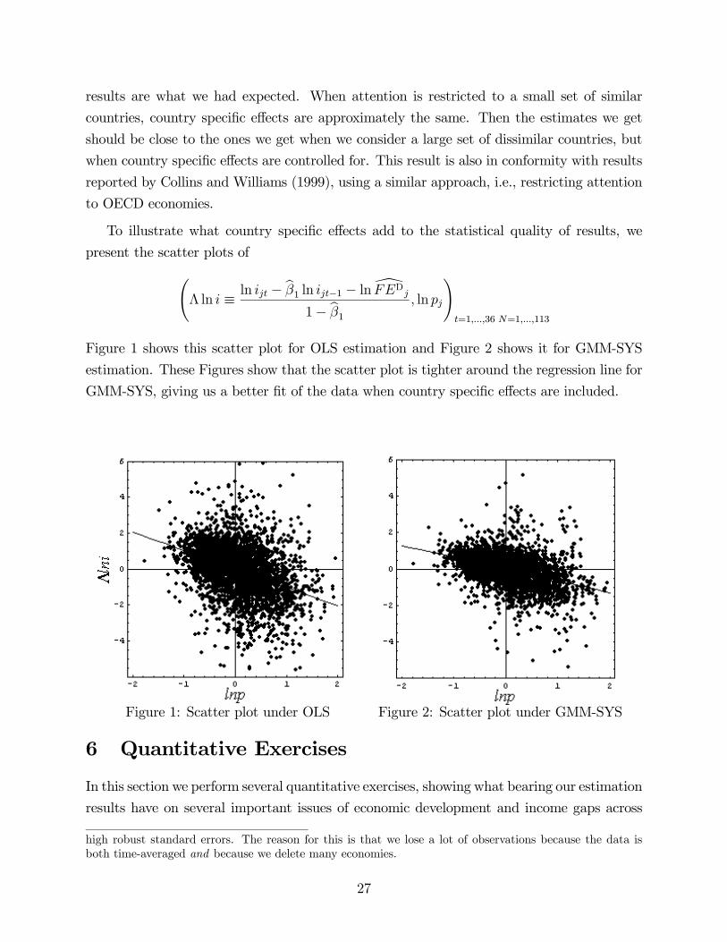
To illustrate what country specific effects add to the statistical quality of results, we

present the scatter plots ofÃΛ ln i ≡ ln ijt −

bβ1 ln ijt−1 − ln[FEDj1− bβ1 , ln pj

!t=1,...,36 N=1,...,113

Figure 1 shows this scatter plot for OLS estimation and Figure 2 shows it for GMM-SYS

estimation. These Figures show that the scatter plot is tighter around the regression line for

GMM-SYS, giving us a better fit of the data when country specific effects are included.

Figure 1: Scatter plot under OLS Figure 2: Scatter plot under GMM-SYS

6 Quantitative Exercises

In this section we perform several quantitative exercises, showing what bearing our estimation

results have on several important issues of economic development and income gaps across

high robust standard errors. The reason for this is that we lose a lot of observations because the data isboth time-averaged and because we delete many economies.

27

countries. In Subsection 6.1 we make the point that if we compare our estimated σ, σ = 0.7,

to the traditionally used σ, σ = 1, then our σ magnifies the effect of distortions and thereby

improves the neoclassical model’s capability to explain income differences. In Subsection 6.2

we perform a development decomposition exercise à la Hall and Jones (1999). This exercise

suggests that σ = 0.7 reduces the correlation between TFP and per capita incomes and again

magnifies the role of distortions. In Subsection 6.3 we assess how much of the distortions

that our model formulation is based on are captured by the investment good price in the

Summers Heston data set.

6.1 How income jointly varies with P and σ

In this subsection we show the quantitative effects of distortions. We calibrate the model to

US data, then show the range and the elasticity of per capita incomes in a simulated model.

The simulated model is the same as the calibrated US model economy, except that we plug

hypothetical values of the distortion parameter into it. We exhibit the simulated model for

various values of σ. This shows that a smaller value of σ magnifies the effect of distortions (in

a sense to be made precise below). Altogether our estimation results along with the analysis

in this subsection suggest that the role of distortions in explaining income gaps is bigger than

has hitherto been believed. Or, to put the matter somewhat differently, they suggest that

policies that reduce distortions in poor economies would have greater stimulative effects.

The analysis in Section 2 shows that steady state per capita income depends on the

distortion parameters TI and TK, on the productivity parameters A and B and on other

parameters of the model. To show this dependence let’s solve (11), assuming an interior

solution. We get

k =

(α

1− α

"µP

P (σ)

¶σ−1− 1#)− σ

σ−1

, (31)

where

P (σ) ≡ Aασ

σ−1

ρ+ δand P ≡ TITK

B. (32)

This solution is interior, i.e., k > 0 if and only if σ < 1 and P < P (σ) or σ > 1 and

P > P (σ).36

36If σ < 1 and P ≥ P (σ) capital demand drops to zero (the economy is poverty trapped), whereas, ifσ > 1 and P ≤ P (σ), capital demand is unbounded.

28

Substituting (31) into (3) and recalling that y = Af (k), we get

y (P,σ) = A

·1− α

1− αK(P )

¸ σσ−1, (33)

where

αK (P ) ≡ kf0 (k)f (k)

=

·P

P (σ)

¸1−σ(34)

is the capital share of income.

Log-differentiating (33), the elasticity of income with respect to distortions is written as

η (P,σ) ≡ −Py

dydP

= σαK (P )

1− αK (P ). (35)

As they stand (33) and (35) depend not only on P and σ but also on other parameters,

namely α andA. To isolate the role of P and σ, we pin down the values of other parameters by

calibrating the model to US data. To do this consider three equations that map unobserved

parameters to observed variables.

y = Ah1− α+ αk

σ−1σ

i σσ−1

αK =α

(1− α) k−σ−1σ + α

(36)

κ ≡ ky=

k

A³1− α+ αk

σ−1σ

´ σσ−1.

y, αK and κ in these equations have the status of observed variables (from US data), while

A and α have the status of unobserved parameters. σ has the status of a “free parameter.”

We normalize y = 1 and solve system (36) for A and α in terms of κ, αK and σ, which gives

A =

hαK + (1− αK)κ

σ−1σ

i σσ−1

κ(37)

and

α =αK

αK + (1− αK)κσ−1σ

. (38)

Furthermore, using (34) and substituting (37) and (38) into (32) we get (subscript C stands

for ‘calibrated’)

PC(σ) =α

σσ−1K

ρ+ δ

1

κand PC =

αKρ+ δ

1

κ. (39)

29

Having solved for A and α we simulate the model, i.e., we ask what US per capita income

would have been for hypothetical values of the distortion parameter, P . We let P = PCP,

where P is a hypothetical distortion parameter for the US economy. We substitute (39) into

(34), which gives

αK(P) = αKP1−σ. (40)

Then we substitute (40) into (33) and (35), and get

y (P,σ) =

µ1− αK

1− αKP1−σ

¶ σσ−1

(41)

and

η (P,σ) = σαKP

1−σ

1− αKP1−σ. (42)

Equations (41) and (42) is what we call the simulated model. They are illustrated in

Figures 3 and 4 for a range of P values for which the solution is interior. The figures illustrate

the dependence of per capita income on distortions for three distinct values of σ: σ = 0.25,

1, and 4.

Figure 3: Output Figure 4: Elasticity

Figures 3 and 4 suggest two ways of determining whether a smaller σ magnifies the effect

of distortions or dampens them. Consider Figure 3 first. Then the (length of the) range

of incomes that is spanned as P varies over some ‘relevant’ domain measures the impact of

distortions. The bigger is this range the greater is the impact of distortions. We will take

the relevant domain to be [1,Pmax], where the high end of the domain Pmax is the largest P

for which the equilibrium is interior. We take the low end of the domain to be 1 because

30

most economies have a calibrated value of P above 1. Altogether whether σ magnifies the

effect of distortion is measured via

l(σ) = y(1,σ)− y(Pmax,σ).

Using this measure and inspecting Figure 3 we see that l is decreasing in σ and thus that

a smaller σ magnifies the effect of distortions.

Figure 4 suggests another way of determining whether a smaller σ magnifies the impact

of distortions. If a smaller σ increases η we say that it magnifies the impact of distortions;

otherwise it dampens it. As Figure 4 shows (and unlike Figure 3) this measure is ‘local’,

i.e., it depends on the particular P at which this effect is evaluated. If P is small, then a

large σ magnifies the impact of distortions.37 On the other hand, if P is large, then a small

σ magnifies the impact of distortions. The analytical counterpart to this is the following

Proposition.

Proposition 1 There exists a P so that

∂η

∂σ≶ 0 iff P ≷ P.

Proof. Differentiating (42) we get

∂η

∂σ= η (P)2

1− αKP1−σ − lnPσ

αKP1−σ.

Therefore the sign of ∂η∂σdepends on the sign of the numerator. Let us study then the numer-

ator, which is a continuous function of P

H (P) ≡ 1− αKP1−σ − ln Pσ. (43)

We prove first that H is decreasing in P whenever the solution is interior. Indeed

dH (P)dP

≡ − σ

Pσ

·1− σ

σαK +P

σ−1¸.

And this is negative when σ < 1 and P < α1

σ−1K or when σ > 1 and P > α

1σ−1K (which, it can

be shown, is equivalent to the condition for interior maximum).

37This finding is consistent with Mankiw’s (1995) work.

31

Second if σ = 1, H (P) ≡ 1 − αK − lnP, so we can explicitly solve H (P) = 0 and get

P = e1−αK . If σ < 1, we have limP&0H (P) = ∞ and H(α1

σ−1K ) = σ

1−σ lnαK < 0. Thus

there must be a P ∈ [0,α1

σ−1K ) so that H

¡P¢= 0. If σ > 1, H(α

1σ−1K ) = − σ

σ−1 lnαK > 0 and

limP%∞H (P) = −∞. So again there must be a P so that H¡P¢= 0. Since H is decreasing

this P is unique.

Given this Proposition we know there must be a bP so that η(bP, 0.7) = η(bP, 1.0), andafter some computations we find that bP = 2.01. Therefore, if P > 2.01 distortions under

σ = 0.7 have stronger impact than under CD, σ = 1. Furthermore, using the calculations

in subsection 6.3, we find that roughly 40% of the (poorest) economies in the PWT have

distortions in this range. The practical implication from this is that policies that reduce

distortions in such economies have a greater impact under a CES production function with

σ = 0.7 than under a CD production function with σ = 1.0.

6.2 TFP when σ = 0.7

In this section we calculate the total factor productivity implied by our model and how it

correlates with per capita incomes. We do this in our model with σ = 0.7, and compare the

results to those calculated by Hall and Jones (1999), which use the Cobb-Douglas specifica-

tion, σ = 1. Hall and Jones (1999) use data for per worker capital and per worker output

controlled for education for 127 economies and measured in efficiency units. The data is for

1988 and the per worker output excludes the output of the mineral sector. We use the same

data for the exercise of this section.

The analogue of the Hall-Jones exercise in our framework works as follows. We substitute

(37) and (38) into the production function and get

yj = Aj

"1− αK + αK

µkjκ

¶σ−1σ

# σσ−1

, (44)

where Aj ≡ AjAis the TFP of the jth economy, A is the US calibrated value from Subsection

6.1, αK = 13and κ = 3 (observed US values).

32

Figure 5: TFP with σ = 1.0 Figure 6: TFP with σ = 0.7

Then we take the values of yj and kj as reported in Hall and Jones (1999). Plugging

those into equation (44), we compute the implied Aj for each economy. Then we plot those

implied Aj against the corresponding GDP’s yj. The plot we get along with the plot that

Hall and Jones get are shown in Figures 5 and 6.

Inspecting these figures and doing some calculations two features are revealed. First the

correlation between the implied A and y is reduced: corr(y,A) is now (under σ = 0.7) 0.49,

whereas before (under σ = 1) it was 0.86. Second the average implied A increases from 0.61

to 0.73.

6.3 How much of the distortions are captured by S-H data?

The model formulation in Section 2 accommodates both observed (TI,j) and unobserved

(TK,j) distortions. This raises the question what portion of the overall distortions are reflected

by the price of capital in the Summers Heston data set. As it turns out, our estimation results

can be used to address that question. To do this, note that equation (18) implies

FEjFEUS

=

µTK,USTK,j

¶σ µAUSAj

¶1−σ,

which, after some manipulations, gives

TK,jTK,US

=

µFEUSFEj

¶ 1σ

A1−σσj . (45)

33

We plug the implies values of Aj (as we computed them in Subsection 6.2) along with the

estimated values of the fixed effects FEj (using the dynamic panel data approach, Subsection

4.2) into (45).38 Then we compute the implied value of TK,j. We find that TK,j ∈ [0.4, 12],that average(TK,j) = 1.5 and that var (lnA) cov (lnA, lnTK) cov (lnA, lnp)

cov (lnA, lnTK) var (lnTK) cov (lnTK, lnp)

cov (lnA, lnp) cov (lnTK, lnp) var (lnp)

= 0.16 −0.08 −0.05−0.08 0.43 0.08

−0.05 0.08 0.24

,where p is the vector of cross time price averages. Looking at this table we see that the cross-

country variability of the PWT data on prices var(lnp), 0.24, represents roughly 36% of the

total cross country variability of incentives to the investment decision, var(lnTK)+var(lnp),

0.67.

For completeness we have done an analogous exercise using the estimated FE from the

static 6 years averaged panel. The results are in the same ball park: TK,j ∈ [0.37, 14],average(TK,j) = 1.7, var(lnTK) = 0.50, cov(lnA, lnTK) = −0.09, cov(lnTK, lnp) = 0.10

andvar (lnp)

var (lnTK) + var (lnp)=

0.24

0.24 + 0.50= 0.33.

Interestingly, when we do the same exercise under a Cobb-Douglas specification, σ = 1.0,

we get the significantly larger portion 66%.

7 Conclusion

This paper presents several econometric exercises aimed at estimating the elasticity of sub-

stitution between capital and labor of an aggregate production function. Our results indicate

that this elasticity hovers around 0.7 and that it is decidedly less than 1. Once we obtain

a value for σ we use it to address the question whether the neoclassical model accounts for

income gaps and to do various macro-development exercises. More broadly, our approach

is to estimate some parameter from data that is relevant to the problem at hand and then

show the role that this parameter plays in a calibration exercise. Let us now suggest that

this approach can be fruitfully applied in other contexts.

The first application is still within the macro-development context. Following up on

Lewis (1954) work, two sector models of development have recently been popularized; see

38We used the SYS-GMM estimates of lnFEDj , and set lnFEj =lnFED

j

1−β1 .

34

for example Hansen and Prescott (2002). One sector is a traditional or agricultural sector

whereas the other is a modern or industrial sector. In such context one studies how economies

transit from traditional to industrial production or, conversely, how poorly managed (highly

distorted) economies revert back to traditional production. Just as above, a key determinant

of this process is the elasticity of substitution and hence one can quantitatively evaluate the

process under an empirically estimated σ. Compared to what we have done here, in this two

sector framework there may no longer be such thing as a poverty trap (which happens in our

one sector model). Compared with the previously studied two sector model, the calibration

and simulation results are expected to be different when σ = 0.7 (as opposed to σ = 1).

A second application is to the (micro) policy question of quantifying the effects of in-

vestment tax credits. The investment equation we derive here, (17), shows that investment

tax credits have a greater stimulative effect on investment the greater is σ. Then, as in

Chirinko (2002), one can study how government policy along with properties of the produc-

tion function affect investments. A third application of our approach is in the context of

the real business cycle literature. A key ingredient in this literature is the aggregate pro-

duction function. Therefore whatever quantitative exercises are done in this literature can

be re-done by first estimating a production function from relevant data and then using it in

the quantitative exercises.

35

References

[1] Alvarez, Javier and Manuel Arellano 2002. “The Time Series and Cross-

Section Asymptotics of Dynamic Panel Data Estimators.” Forthcoming in Econometrica

(http://www.cemfi.es/~arellano/#WPapers).

[2] Arellano, Manuel 1987. “Computing Robust Standard Error for Within Groups.”Oxford Bulletin of Economics and Statistics, 49: 431-434.

[3] Arellano, Manuel, and Stephen Bond 1991. “Some Tests of Specification for PanelData: Monte Carlo Evidence and an Application to Employment Equations.” Review

of Economic Studies, 58: 277-297.

[4] Arellano, Manuel, and Stephen Bond 1998. “Dynamic Panel Data Estimationusing DPD98 for Gauss: A Guide for Users” Institute for Fiscal Studies, London

(http://www.ifs.org.uk/staff/steve_b.shtml).

[5] Arellano, Manuel, and Olympia Bover 1995. “Another Look at the InstrumentalVariables Estimation of Error Components Models.” Journal of Econometrics, 68: 29-

51.

[6] Arrow, K. J., H. B. Chenery, B. S. Minhas and R. M. Solow 1961. “Capital-Labor Substitution and Economic Efficiency.” Review of Economic and Statistics, 43(3):

225-250.

[7] Baltagi, Badi 1995. Econometric Analysis of Panel Data. New York: John Wiley &Sons.

[8] Bhargava, A., L. Franzini, and W. Narendranathan 1982. “Serial Correlationand the fixed effects model.” The Review of Economics Studies, 49: 533-549.

[9] Blundell, Richard, and Stephen Bond 1998a. “Initial Conditions and MomentRestrictions in Dynamic Panel Data Models.” Journal of Econometrics, 87: 115-14

[10] Blundell, Richard, and Stephen Bond 1998b. “GMM Estimation with Persistent

Panel Data: an Application to Production Functions.” The Institute for Fiscal Policies,

Working Paper Series No W99/4 (http://www.ifs.org.uk/working papers/wp994.pdf).

[11] Bond, Stephen, Anke Hoeffler, and Jonathan Temple 2001. “GMM

Estimation of Empirical Growth Models.” Discussion Paper # 01/21

(http://www.nuff.ox.ac.uk/economics/papers/2001/w21/bht10.pdf).

36

[12] Chamberlain, Gary 1984. “Panel Data,” in: Handbook of Econometrics, Vol 2, Eds:Z. Griliches and M. D. Intriligator, Elsevier, Amsterdam, 1247-1313.

[13] Chirinko, Robert S. 2002. “Corporate Taxation, Capital Formation,

and the Substitution Elasticity Between Labor and Capital.” Emory Uni-

versity, Department of Economics Working Papers # 02-01 (March)

(http://userwww.service.emory.edu/%7Eskrause/wp/chirinko_02_01_cover.htm).

[14] Chirinko, Robert S., Steve M. Fazzani and Andrew P. Mayer 2002. “That Elu-sive Elasticity: A Long Panel Approach to Estimating The Price Sensitivity of Business

Capital.” Emory University, Department of EconomicsWorking Papers # 02-02 (March)

(http://userwww.service.emory.edu/%7Ecozden/chirinko_02_02_cover.html).

[15] Collins, Williams J. and Jeffrey G. Williams 1999. “Capital Goods Prices, GlobalCapital Markets and Accumulation: 1870-1950.” NBERWorking Paper No. 7145 (May).

[16] Hall, Robert, and Charles Jones 1999. “Why Do Some Countries Produce So MuchMore Output per Worker Than Others?” Quarterly Journal of Economics, 114(1): 83-

116.

[17] Hansen, Gary and Edward Prescott 2002. “Malthus to Solow.” American Eco-nomic Review, 92(4): 1205-1218.

[18] Heston, Alan, Robert Summers and Betina Atten 2002. “Penn-World TableVersion 6.1.” Center for International Comparisons at the University of Pennsylvania,

October (http://pwt.econ.upenn.edu/).

[19] Holtz-Eakin, Douglas, White Newey, and Harvey Rosen, 1988. “EstimatingVector Autoregressions with Panel Data.” Econometrica, 56(6): 1371-1395.

[20] Hsieh, Chang-Tai and Peter J. Klenow 2003. “Relative Prices and Relative Pros-perity.” Working Paper (April) (http://www.klenow.com/).

[21] Jones, Charles I. 1994. “Economic Growth and the Relative Price of Capital.” Jour-nal of Monetary Economics, 34: 359-382.

[22] Judson, Ruth, and Ann Owen 1996. “Estimating Dynamic Panel Data Models: APractical Guide for Macroeconomists.” Federal Reserve Board of Governors.

[23] Klenow, Peter J. and Andrés Rodríguez-Clare 1997. “The Neoclassical Revivalin Growth Economics: Has It Gone Too Far?” NBER Macroeconomics Annual, Ben S.

Bernanke and Julio J. Rotemberg (editors), The MIT Press: 73-103.

37

[24] Loayza, Norman, Klaus Schmidt-Hebbel, and Luis Serven 2000. “What DrivesPrivate Saving Across the World?” Forthcoming, Review of Economics and Statistics.

[25] Lucas, R. E., Jr. 1969. “Labor-Capital Substitution in US Manufacturing.” in TheTaxation of Income from Capital, ed. Arnold C. Harberger and Martin J. Bailey, The

Brookings Institution, Washington, D.C.

[26] Lewis, W. A. 1954. “Economic Development with Unlimited Supplies of Labor.”Manchester School of Social Science, 22: 139-191.

[27] Maddala, G. S. and I. Kim 1998. “Unit Roots, Cointegration and StructuralChange.” Cambridge: Cambridge University Press.

[28] Mankiw, N. Gregory 1995. “The Growth of Nations.” Brookings Papers on Eco-nomic Activity, 1995 (1): 275-326.

[29] Nickell, Stephen 1981. “Biases in Dynamic Models with Fixed Effects.” Economet-rica, 49(6): 1417-1426.

[30] Parente, Stephen and Edward Prescott 2000. Barriers to Riches. The MIT Press:Cambridge, Massachusetts.

[31] Pessoa, Samuel and Rafael Rob 2003. “The Implications of Embodiment andPutty-Clay to Economic Development,” Mimeo, University of Pennsylvania.

[32] Romer, David 2001. Advanced Macroeconomics, Second Edition, McGraw-Hill.

[33] Restruccia, Diego and Carlos Urritia 2001. “Relative Prices and InvestmentRates.” Journal of Monetary Economics, 47: 93-121.

[34] Summers, Robert and Alan Heston 1991. “The Penn-World Table: An ExpandedSet of International Comparisons, 1950-1988.” Quarterly Journal of Economics 106

(May): 327-368.

[35] Windmeijer, Franck 2000. “A Finite Sample Correction for the Variance of LinearTwo-Step GMM Estimators.” The Institute of Fiscal Policies, Working Paper Series n.

W00/19.

38

A Dynamic panel Estimation with GMM

GMM-DIF Estimation. The first two observations used for estimating equation (24) arelost to lags and differencing. At t = 3, ln ij1 is a valid instrument for ln ij2 − ln ij1, andln pj1 is a valid instrument for ln pj2− ln pj1 and ln pj3− ln pj2. Similarly, at t = 4, ln ij1 andln ij2 are valid instruments for ln ij3 − ln ij2, and ln pj1 and ln pj2 are valid instruments forln pj3 − ln pj2 and ln pj4 − ln pj3, respectively. Consequently, the instrument matrix has onerow for each time period, giving T − 2 rows altogether, and M = 2 ×

T−2Pm=1

m columns. The

instruments matrix is

ZDj =³ZD1j , Z

D2j

´,

where

ZD1j =

ln ij1 0 0 0 · · · 0 0 0

0 ln ij1 ln ij2 0 · · · 0 0 0...

......

. . ....

......

...

0 0 0 · · · ln ij1 ln ij2 · · · ln ijT−2

,

ZD2j =

ln pj1 0 0 0 · · · 0 0 0

0 ln pj1 ln pj2 0 · · · 0 0 0...

......

. . ....

......

...

0 0 0 · · · ln pj1 ln pj2 · · · ln pjT−2

.Let Xjt = (ln ijt−1, ln pjt, ln pjt−1) be the 1 × 3 vector of covariates for j and t and Θ the

3× 1 vector of coefficients. Define the first-differenced variables as

y∗j =

ln ij3 − ln ij2ln ij4 − ln ij3

...

ln ijT − ln ijT−1

, X∗j =

Xj3 −Xj2

Xj4 −Xj3

...

XjT −XjT−1

, and ²∗j =

²j3 − ²j2²j4 − ²j3

...

²jT − ²jT−1

.

The moment restrictions (25) and (26) can be written as E(ZD0j ²∗j) = 0, where 0 is anM ×1

vector of zeros. The GMM estimator based on these moment restrictions minimizes the

expected quadratic distance between ²∗0ZDWZD0²∗ and the true vector of parameters for

the metricW, where ZD0 is theM×N(T−2) matrix (ZD01 ,ZD02 , ..ZD0N ) and ²∗0 is the N(T−2)

39

vector (²∗01 , ²∗02 , ...²

∗0N). This gives the GMM estimator of Θ as

bΘ = (X∗0ZDWZD0X∗)−1X∗0ZDWZD0y∗,

where y∗0 is an N(T − 2) vector and X∗ is an N(T − 2)× 3 matrix.Arellano and Bond (1991) suggest two choices for the weights W, giving rise to two

GMM estimators: one and two step estimators. In the one step estimator it is assumed

that the ²jt are independent and homoskedastic both across units and over time. Then the

optimal choice ofW is given byW1 = (1N

NPj=1

ZD0j HDZDj )

−1, whereHD is the (T−2)×(T−2)variance-covariance matrix of E(²∗j²

∗0j )

HD =

2 −1 0 · · · 0 0

−1 2 −1 · · · 0 0...

......

. . ....

...

0 0 0 · · · 2 −10 0 0 · · · −1 2

.

The variance-covariance estimator of the parameter bΘ that is robust to heteroskedasticity isdV C(Θ) = N(X∗0ZDW−1ZD0X∗)−1X∗0ZDW−1(

NXj=1

ZD0j b²∗jb²∗0j ZDj )W−1ZD0X∗(X∗0ZDW−1ZD0X∗)−1,

where b²∗j are the estimated residuals.For the two step estimator the previous assumptions about ²jt are relaxed. In the first

step we obtain the b²∗j and then we use them to construct a consistent estimate of the variance-covariance matrix of the moment restrictions. In this case, the optimal choice ofW is given

byW2 = (1N

NPj=1

ZD0j b²∗jb²∗0j ZDj )−1.Both GMM estimators are consistent when N is much larger than T , although they may

differ in their asymptotic efficiency. Also, in the special case of i.i.d. disturbances, both are

asymptotically equivalent.

System GMM. The additional moment conditions (27) and (28) can be expressed as

E(ZL0²j) = 0,

where

40

ZLj =

y∗j2 0 · · · 0

0 y∗j3 · · · 0...

.... . .

...

0 0 · · · y∗jT−1

4 ln pj2 0 · · · 0

0 4 ln pj3 · · · 0...

.... . .

...

0 0 · · · 4 ln pjT−1

,with 4 ln pjt = ln pjt − ln pjt−1. Now, we can construct a GMM estimator which exploits

both sets of moment restrictions. The instrument matrix for GMM-SYS is written as

Zj =

ÃZDj 0

0 ZLj

!.

The GMM-SYS estimator combines both sets of moment restrictions

E(Z0jξj) = 0,

where

ξj =

ò∗j²j

!.

Note that the one step GMM estimator is not asymptotically equivalent to the two step

estimator - even when disturbances are i.i.d. The natural candidate for a weighting matrix

for the one step estimator isWSY S1 = ( 1

N

NPj=1

Z0jHZj)−1, where H is

Hj =

ÃHDj 0

0 Ij

!,

which is always asymptotically inefficient relative to the two step estimator, because with

level equations included in the system, the optimal weighting matrix depends on unknown

parameters.

The construction of the two step GMM-SYS estimator is then analogous to that described

under GMM-DIF, except that we use Hj = bξj bξj 0.Monte Carlo simulations of Blundell and Bond (1998a) show that the finite sample dis-

tributions of the one step and two step system GMM estimators are similar.

41

B Estimated Standard Error of the Long-Run Price

Elasticity

In order to compute the estimated standard error of the long run price elasticity of investment

demand βLR we apply the Delta Method. Define β ≡ (β1,β2, β3)0. Then βLR, as a function

of β, is given by equation (23). Applying a first order Taylor series approximation to this

function around the true value of β we get

LR(bβ1, bβ2, bβ3) ≈ LR(β1, β2,β3) + (∇LR)0(bβ − β), (46)

where

(∇LR)0 =h

β2+β3(1−β1)2 ,

11−β1 ,

11−β1

iis the gradient of LR(β1,β2, β3). The variance of LR(bβ1, bβ2, bβ3) (which is a nonlinear functionof (bβ1, bβ2, bβ3)) is approximately equal to the variance of the right hand side of (46), which is

var(LR(bβ1, bβ2, bβ3)) = ∂LR∂β

|β=bβvar(bβ)∂LR∂β|0β=bβ ,

where var(bβ) is the estimated variance-covariance matrix of βvar(bβ) =

var(bβ1) cov(bβ1, bβ2) cov(bβ1, bβ3)cov(bβ1, bβ2) var(bβ2) cov(bβ2, bβ3)cov(bβ1, bβ3) cov(bβ2, bβ3) var(bβ3)

.C The Bias of the OLS Estimation

We assume in this Appendix that the price of investment is an exogenous variable. Then

bβBias = plimN→∞

µ1

NX0X

¶−11

NX0FE, (47)

where

X03×((T−1)N)

=

1 . . . 1

ln i12 . . . ln i1T

ln p12 . . . ln p1T

· · ·1 . . . 1

ln ij2 . . . ln ijT

ln pj2 . . . ln pjT

· · ·1 . . . 1

ln iN2 . . . ln iNT

ln pN2 . . . ln pNT

42

and

FE01×((T−1)N)

=hlnFE

D1 . . . lnFE

D1 · · · lnFE

Dj . . . lnFE

Dj · · · lnFE

DN . . . lnFE

DN

i.

lnFEDj ≡ lnFEDj − 1

N

NPj0=1

lnFEDj0 is the centred fixed effect for the j-th economy. The first

observation is deleted due to the dynamics.

Evaluating 1NX0FE, we have

1

NX0FE =

1N

NPj=1

lnFEDj

1N

NPj=1

TPt=2

ln ijt lnFEDj

1N

NPj=1

TPt=2

ln pjt lnFEDj

.

Now we are going to compute each of the three components of 1NX0FE. The first component

is zero by the way lnFEDj is defined. It remain then to compute the other two components.

To compute the third component of 1NX0FE, we assume that the covariance between the

price and the fixed effect is time invariant

plimN→∞

1

N

NXj=1

ln pjt lnFEDj = plim

N→∞

1

N

NXj=1

ln pjt0 lnFEDj for any t, t

0 ∈ {1, ..., T} . (48)

Then

plimN→∞

1

N

NXj=1

TXt=2

ln pjt lnFEDj = plim

N→∞

T − 1N

NXj=1

ln pj lnFEDj .

To compute the second component of 1NX0FE, we apply equation (22) in the text. Then,

using σ = −β2+β31−β1 and the fact that β3 is estimated to be zero, equation (22) is reduced to

ln ijt = lnFEDj + β1 ln ijt−1 − σ (1− β1) ln pjt + ²jt. (49)

Now we repeatedly substitute (49) into itself, obtaining

ln ijt =1− βt−11

1− β1lnFEDj + βt−11 ln ij1 −

t−2Xk=0

βk1 [σ (1− β1) ln pj,t−k − ²j,t−k] . (50)

43

Then assuming that all economies are initially on a balanced growth path we have

ln ij1 = lnFEDj − σ ln pj1 + ²j1. (51)

Plugging (51) into (50) we get

ln ijt =1− βt11− β1

lnFEDj − βt1σ ln pj1 − σ (1− β1)t−1Xk=0

βk1 ln pj,t−k +t−1Xk=0

βk1²j,t−k.

The above equation allows us to write the second component of 1NX0FE as

NXj=1

TXt=2

ln ijt lnFEDj =

TXt=2

1− βt11− β1

NXj=1

lnFEDj lnFEDj − σ

TXt=2

βt1

NXj=1

ln pj1 lnFEDj

− σ (1− β1)TXt=2

t−1Xk=0

βk1

NXj=1

ln pj,t−k lnFEDj

+TXt=2

t−1Xk=0

βk1

NXj=1

²j,t−k lnFEDj .

To simplify this last expression, we re-use our assumption (48) and, on top of that, assume

that

plimN→∞

1

N

NXj=1

²jt lnFEDj = 0, for all t.

Then after some calculations we find that

plimN→∞

1

N

NXj=1

TXt=2

ln ijt lnFEDj = plim

N→∞

D

N

NXj=1

lnFEDj lnFEDj − plim

N→∞σT − 1N

NXj=1

ln pj lnFEDj ,

where

D ≡ (1− β1) (T − 1)− β21¡1− βT−11

¢(1− β1)

2 .

This completes the computation of the second component. Introducing simplifying notation

and stacking up the three components we have

1

NX0FE =N

0

Dvar¡lnFED

¢− σ (T − 1) cov ¡lnFED, lnp¢(T − 1) cov ¡lnFED, lnp¢

.

44

Going back to (47) we now find that

bβBias = bβ0,Biasbβ1,Biasbβ2,Bias

= µplimN→∞

detX0X

N3 (T − 1)2¶−1 • • •

• var (lnp) −cov (ln i, lnp)• −cov (ln i, lnp) var (ln i)

×

0

Dvar¡lnFED

¢− σ (T − 1) cov ¡lnFED, lnp¢(T − 1) cov ¡lnFED, lnp¢

.Now that we found the biases, we plug them into (30) and derive the following result

∂bβOLSLR

∂cov (FE,p)=

µplimN→∞

detX0X

N3 (T − 1)3¶−1

2− σ + bβOLSLR (1− σ)

1−³bβ1 + bβ1,Bias´ var (lnp) . (52)

In deriving this result we use the fact that, according to the data,

var (ln i) ≈ 2var (lnp) and var (lnp) ≈ −cov (ln i, lnp) .

Consider now equation (52). The first and third terms are positive. The denominator of the

second term is also positive because all our regression results are such that bβ1 + bβ1,Bias <1 (and more generally because unit root in the investment process had been ruled out).

Therefore if we can show that the numerator of the second term is positive we will have that

∂bβOLSLR

∂cov¡lnFED, lnp

¢ > 0.To show that this numerator is positive we note that

−2− σ

1− σ≈ −2−

bβLR1− bβLR = −1.30.3 ≈ −4.

where the equality comes from our estimation result bβLR = 0.7 (see Table 6, column [8]).

Therefore if we can show that 0 ≥ bβOLSLR > −4 we would be done.Let’s then explicitly calculate bβOLSLR . To do that we use the full information from the data

(X0X)−1 =

0.0070 −0.0023 −0.0026−0.0023 0.0008 0.0008

−0.0026 0.0008 0.0016

,45

and the following estimated values from our GMM-SYS estimation

NXj=1

ln pj lnFEDj = −3 and

NXj=1

lnFEDj lnFEDj = 1.5.

Furthermore, the dynamic panel has T = 36 and we know from the GMM-SYS estimation

that bβ1 = 0.744 and bβ2 = −0.177 (Table 6, column [8]). Using all these values we getD ≈ 128 and σ (T − 1) ≈ 25. Then after plugging this into equation (30) we get

bβOLSLR =bβ2 + bβ2,Bias

1−³bβ1 + bβ1,Bias´ = −1.04,

where bβ1,Bias = 0.13 and bβ2,Bias = 0.042.

46