Identifying Extreme Cold Events Using Phase Space ...

Identifying Extreme Cold Events Using Phase SpaceReconstruction

Babatunde I. Ishola*, Richard J. Povinell,George F. Corliss, and Ronald H. BrownDeparment of Electrical and Computer Engineering,Marquette University,P.O. Box 1881, Milwaukee, WI 53201-1881, USAE-mail: [email protected]: [email protected]: [email protected]: [email protected]*Corresponding author

Abstract: Extreme cold events in natural gas demand are characterized by unusualdynamics that makes modeling the characteristics of the gas demand duringextreme cold events a challenging task. This unusual dynamics is in the formof hysteresis, possibly due to human behavioral response to extreme weatherconditions. To natural gas distribution utilities, extreme cold events representhigh risk events given the associated huge demand of gas by their customers.To understand the nature of the unusual dynamics and help utilities in theirdecision-making process, we present a semi-supervised learning algorithm thatidentifies extreme cold events in natural gas time series data. Using phase spacereconstruction, the input space is mapped into a phase space. In the reconstructedphase space, events with similar dynamics are closer together, while events withdifferent dynamics are far apart. A cluster containing extreme cold events isidentified by finding the nearest neighbors to an observed cold event. The learningalgorithm was tested on natural gas consumption data obtained from naturalgas local distribution companies. Our RPS-kNN algorithm was able to identifyextreme cold events in the data.

Keywords: Reconstructed Phase Space; Nearest Neighbor; Semi-supervisedlearning; Extreme Cold Events; and Energy Forecasting.

Reference to this paper should be made as follows: Ishola, B., Povinelli, R.,Corliss, G. and Brown, R. (2016) ‘Identifying Extreme Cold Events Using PhaseSpace Reconstruction’, Int. J. Applied Pattern Recognition, Vol. x, No. x, pp.xx-xx.

Biographical notes: Babatunde Ishola is pursuing an M.S. degree in Electricaland Computer Engineering at Marquette University. He received his B.S. degreein Electronic and Electrical Engineering from Obafemi Awolowo University,Nigeria, in 2012. He is currently a supported Graduate Research Assistant on theGasDay Project at Marquette University.

Richard J. Povinelli received the B.S. degree in electrical engineering and B.A.degree in psychology from the University of Illinois, Champaign-Urbana, IL,USA, in 1987, the M.S. degree in computer and systems engineering fromRensselaer Polytechnic Institute, Troy, NY, USA, in 1989, and the Ph.D. degree

Copyright © 2016 Inderscience Enterprises Ltd.

2

in electrical and computer engineering from Marquette University, Milwaukee,WI, USA, in 1999. From 1987 to 1990, he was a Software Engineer with GeneralElectric (GE) Corporate Research and Development. From 1990 to 1994, hewas with GE Medical Systems, where he served as a Program Manager andthen as a Global Project Leader. From 1995 to 2006, he consecutively held thepositions of Lecturer, Adjunct Assistant Professor, and Assistant Professor withthe Department of Electrical and Computer Engineering, Marquette University,Milwaukee, WI, USA, where, since 2006, he has been an Associate Professor.His research interests include signal processing, machine learning, and chaosand dynamical systems. He has authored and coauthored over 60 publications inthese areas.

George Corliss is professor of electrical and computer engineering at MarquetteUniversity and Senior Scientist of the GasDay Project. He received his B.A. inmathematics for the College of Wooster (Ohio) and his Ph.D. in mathematicsfrom Michigan State University. He has taught and worked at the University ofNebraska, Lincoln, University of Wisconsin, Madison, Swiss Federal Instituteof Technology, Argonne National Laboratory, Karlsruhe Institute of Technology(Germany), Compuware Corp., and Marquette University, as well as in severalindustrial and consulting positions. His research interests include scientificcomputation and mathematical modeling, guaranteed enclosures of the solutionsof ordinary differential equations, industrial applications of mathematics andscientific computation, numerical optimization, automatic differentiation, andsoftware engineering. He teaches courses in engineering design, computerarchitecture, operating systems, database design, and software engineering.

Dr. Ronald H. Brown is Associate Professor of Electrical and ComputerEngineering at Marquette University and the founding Director of MarquetteUniversityâŁ™s GasDay Project. Dr. BrownâŁ™s research is in systemmodeling, identification, prediction, optimization, and control. The applicationsof his research has been focused on natural gas distribution and transmission since1993, when the GasDay Project was founded as a means to connect students withthe many industrial partners who support the labâŁ™s work. Over the course ofthe project he has worked with more than 150 undergraduate students from fourcolleges at Marquette directly participating in the project, and many more whohave participated through classroom assignments that have âŁžborrowedâŁžproject ideas from GasDay. He is a frequent presenter at energy industry meetingsand consultant to many energy companies looking for guidance in planning fordaily and peak load conditions.

1 Motivation

The most important days in natural gas demand forecasting include the days when demandis at its peak. It is important to forecast gas demand accurately during this period because ithelps in infrastructure, supply, and operational planning (Lyness (1981)). Residential andcommercial gas demand increases as the temperature decreases since homes and businessesuse more natural gas for space heating as it gets colder(Vitullo et al. (2009)). The highestgas demand occurs during extreme cold events. An extreme cold event is a multi-day eventfor which the temperature is below a given threshold (specified by 1-in-n years) for severalconsecutive days with a characteristic response in gas demand in the form of hysteresis(see Figure 1). A 1-in-n temperature denotes the temperature which occurs as infrequentlyas once every n years. Extreme cold events are by nature rare, so they are not represented

Identifying Extreme Cold Events Using Phase Space Reconstruction 3

adequately in gas demand data, leading to high forecast error during extreme cold events.Considering the financial implications as well as physical limits to the amount of gas supplythat can be made available during an extreme cold event, it is important to identify extremecold events in natural gas demand data. Identifying these events enables us to improve thegas demand forecast during such events, which may represent the most challenging daysof the year for operational gas forecasters because their gas delivery systems are operatingnear their maximum capacities.

1.1 Behavioral Response

In addition to the infrequent nature of extreme events, they are also characterized by someinteresting behaviors. Generally, gas demand varies linearly with temperature. For extremecold events however, this relationship becomes non-linear. An unusual response in gasconsumption in the form of hysteresis has been observed during the extreme cold events.Figure 1 shows the plot of daily natural gas consumption (flow) against wind-adjustedtemperature (labeled HDDW), spanning a period of ten years. Figure 1b is a replica ofFigure 1a with emphasis on the behavior of interest. The straight lines connect instances ofnatural gas consumption versus wind-adjusted temperature for five consecutive days. Thedays in the series identified by the lines represents the consumption for days t− 2, t− 1,t, t+ 1, and t+ 2, with t being the coldest day in the event. The flow for the day after thecoldest day (t+ 1) is much higher than the flow for day t, even though the temperature iswarmer. Apparently, people tend to use more gas even when it is not as cold as the daybefore.

Part of this response is due to thermodynamic effects, as heat transfer is a dynamicprocess. There is a certain time-lag relating the reported (outside) temperature to the actualtemperature (inside the building). The lag factor depends on the building’s insulationsystem. Murat (2011) provides a good insight into the effect of thermodynamics on spaceheating in buildings. Attempts have been made to model the thermodynamics componentby adjusting the forecast model for prior day weather effects as shown by Vitullo et al.(2009), and Brown and Matin (1995). The hypothesis here is that there is an unmodeledbehavioral component, possibly due to human responses to extreme temperature and/ortemperature changes (see Kalkstein et al. (1986), Brown (2014a), and Brown (2014b)),since the response to extreme cold events appears different from typical days.

In the next section, we will build a gas demand forecast model and observe the model’sperformance during extreme cold events.

1.2 Gas Demand Forecast Model

This section describes a base line gas demand model that will referenced throughout thispaper. This base model is an ensemble of multiple linear regression (MLR) and artificialneural networks (ANN). The MLR model is a 13-parameter linear regression model

St = β0 +

13∑i=1

βixi,t , (1)

St = St + εt , (2)

where St is the model estimate of gas demand for day t, xi,t represents input features suchas temperature, prior day temperature, wind speed, day of week, and so on, with β being the

4

(a)

(b)

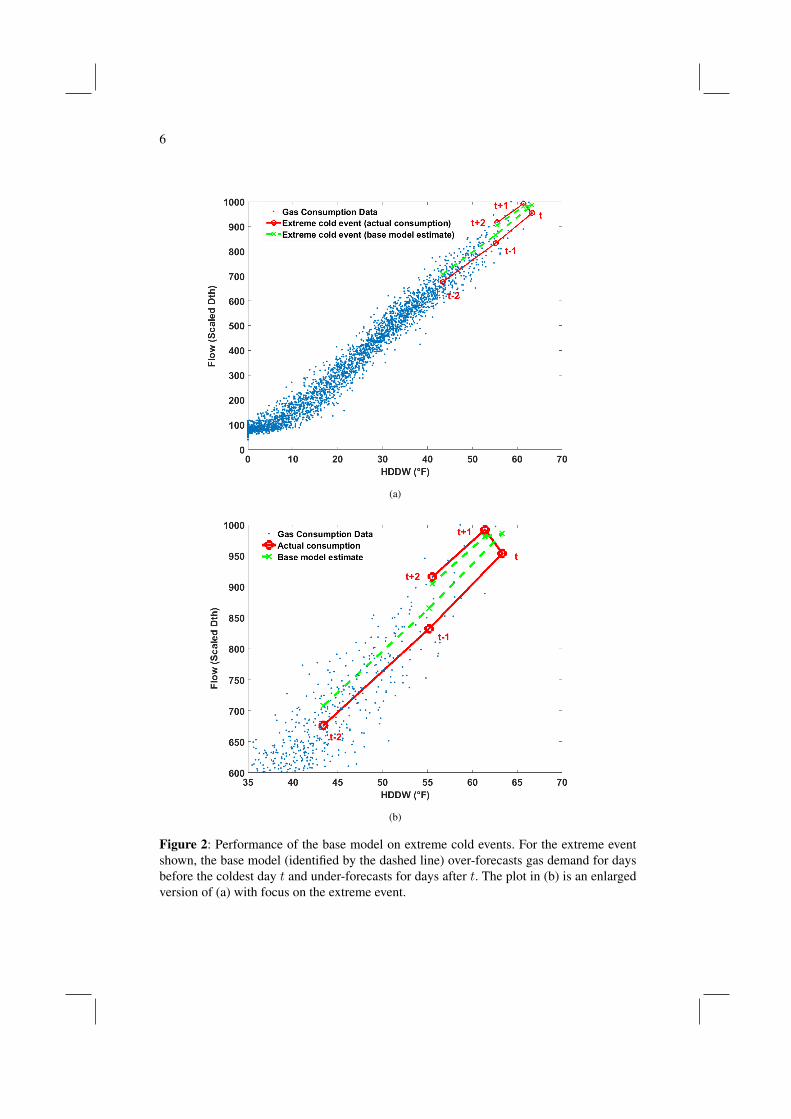
Figure 1: An extreme cold event in natural gas consumption data for a certain region in theUSA. The extreme event identified can be seen to exhibit a hysteresis effect as a result ofunusual (human behavioral) response to extreme temperatures. The plot in (b) is an enlargedversion of (a) with focus on the extreme event.


model parameters. Let εt be the forecast error for day t. Then the actual flow St is relatedto the estimated flow St by Equation 2. The MLR component assumes a linear relationshipbetween the dependent and independent variables, while the ANN model accounts for non-linear responses to the input features. The ANN model uses the same input features as theMLR model. The ensemble model was trained on historical data obtained from gas utilitiesin the USA. The learned model was used to estimate daily gas demand.

1.3 Base Model Performance

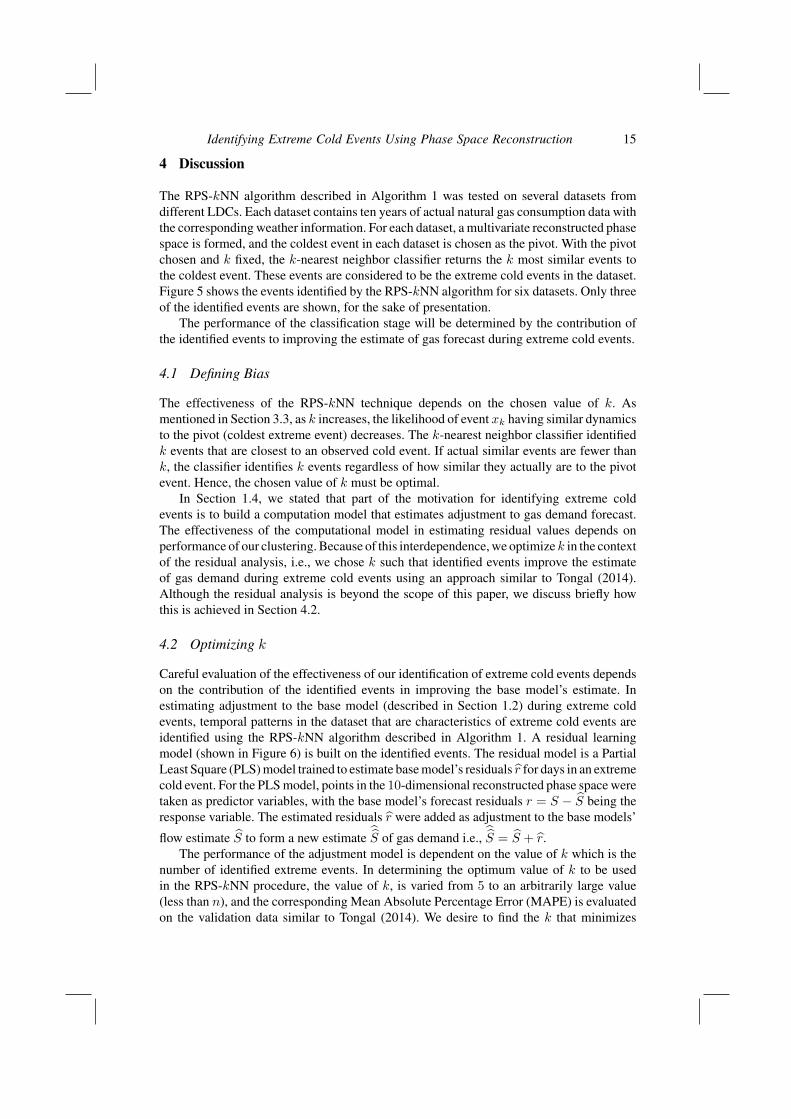
The base model described in Section 1.2 often over-forecasts and under-forecasts gasdemand for days before and after the coldest day in an extreme cold event, respectively.Figure 2a shows an extreme cold event. If t is the index of the coldest day in the extremecold event, on days t, t− 1, and t− 2, the dashed line (base model estimate) is abovethe straight line (actual consumption), which means the demand forecast is more than theactual consumption for days before the coldest day. For days t+ 1 and t+ 2, the dashedline is below the straight line, which means that the gas demand forecast is less than theactual consumption for days after the coldest day. This pattern of demand forecast andunusual response during extreme cold events has been observed for more than 20 operatingareas (from different geographical locations), especially for those areas that have experiencesevere weather conditions in the past 10 years.

1.4 Quantifying Deviation

The work presented in this paper offers a strategy for adjusting the current base modelestimate during extreme cold events to improve the accuracy of the gas demand forecast. Ourstrategy involves quantifying the deviation of the base model (which is a result of unmodeledbehavioral components) from the actual demand during extreme events. A computationalmodel is built based on the statistics of this deviation to estimate the forecast residual onextreme cold events. This is employed to estimate an adjustment to the base model.

To build a computational model that estimates forecast residual on extreme cold events,the extreme events are identified in the data. In Section 1.1, we postulated that extreme coldevents have different dynamics than usual days due to the unusual behavioral response. Inidentifying extreme cold events, we search for events in the data with similar dynamics toa known extreme event. The events are treated as temporal patterns.

We identify temporal patterns in natural gas data that correspond to extreme cold events.This is achieved by clustering the data based on dynamics. Natural gas demand is a highdimensional system, so that events with similar dynamics may not occupy the same clusterin the input data space. For effective clustering, a low-dimensional embedding of the datais performed using phase space reconstruction (Povinelli et al. (2006)). In the reconstructedphase space, events with similar dynamics are closer to each other, while those with differentdynamics are far apart. Extreme cold events are identified by finding the events that are closeto a known extreme cold event in the reconstructed phase space, using a nearest neighboralgorithm.

1.5 Paper Overview

In the next section, we discuss important concepts on which the work presented in this paperis based, such as modeling non-stationary time series and phase space reconstruction forpattern recognition. In Section 3, we describe our approach to identifying temporal patterns

6

(a)

(b)

Figure 2: Performance of the base model on extreme cold events. For the extreme eventshown, the base model (identified by the dashed line) over-forecasts gas demand for daysbefore the coldest day t and under-forecasts for days after t. The plot in (b) is an enlargedversion of (a) with focus on the extreme event.


of extreme cold events in natural gas time series data. Pseudocode also is presented. InSection 4, we discuss the performance of our approach and present results obtained whenthe algorithm was evaluated on six gas demand data sets from different gas utilities. Asfuture work, we provide a brief overview on how the result of the identification is beingused to estimate adjustments to gas forecast on extreme cold days.

2 Forecasting Non-stationary Data

In a non-stationary time series, the statistical properties of the underlying system vary overdifferent regions of the data space. A common technique for forecasting such time seriesdata involves building multiple models, with each model optimized for different regions ofthe data. The data space is partitioned into regions of similar dynamics using some clusteringalgorithm, and local models are learned for each identified cluster. The multiple local modelapproach often achieves higher forecasting accuracy than a single global model (Vilalta etal. (2010)). Global models are only well suited to stationary data, as they attempt to find anapproximate representation of a system’s dynamics (Pavlidis et al. (2006); Cao (2003)).

In financial forecasting, where exchange rates are highly correlated with economic,political, and psychological factors, all interacting in a highly complex manner, Pavlidis etal. (2006) employed clustering algorithms to partition the input data space into subspaces.Each subspace was learned using Feed-Forward Neural Networks (FFNN). Given test data,it was first determined to which cluster the data point belongs, and the corresponding FFNNwas used to predict the exchange rate. Results reported show that the approach compareswell with other established approaches. Cao (2003) employed a mixture of support vectormachine (SVM) experts, with each expert optimized to forecast different regions of theinput space. A self-organizing feature map was developed to cluster the input data space intoseveral disjointed regions. With the partitioned regions having a more uniform distributionthan the original input space, it becomes easier for the SVM experts to capture a stationaryinput-output relationship. The SVM expert that best fits a partitioned region is trained byfinding the most appropriate kernel function and optimal free parameters of the SVM. Usingthree openly available data as test cases, Cao showed that for all the test cases, the mixtureof SVM experts model achieves better performance than a single SVM model Cao (2003).

2.1 Clustering

The performance of the multiple model approach depends on the effectiveness of theclustering step. Clustering algorithms are used in data mining and pattern recognition taskswhere items are to be separated into groups. Items in the same group are considered similar,with similarity defined only in the sense of the particular application. Metrics used indetermining similarity include distance (i.e., how close the points are), density (i.e, howcompact points are), and connectivity. When using a distance function as a similarity metric,it is possible for similar points to be far apart in the input data space, especially whendealing with high dimensional data. In high dimensional spaces, distances between pointsare relatively uniform, so the concept of closeness is meaningless (Steinbach et al. (2004)).In clustering such high-dimensional data, it is customary to perform a low-dimensionalembedding, mapping the input data space into a new space where closeness is properlydefined.

8

2.2 Phase Space Embedding

One common technique employed in low-dimensional embedding of high dimensionaldata is called phase space reconstruction. Phase space reconstruction is based on Takens’(1981) time-delay embedding theorem. Takens’ theorem gives the condition under which adynamical system can be reconstructed from a sequence of observations of the state of thesystem. Sauer et al. (1991) showed that for almost every time delay embedding with theappropriate selection of embedding parameters (dimension and time-lag), the reconstructeddynamics, with a probability of 1, are topologically identical to the true dynamics of theunderlying system. Hence, the underlying dynamics of a system can be captured fully in areconstructed phase space (RPS).

This technique is able to reconstruct the underlying dynamics of any complex systemand map it into a new lower dimensional space. Since the RPS is equivalent to the truedynamics of the system, points with similar dynamics are guaranteed to be close in thisspace, while less similar points are far apart (Povinelli et al. (2004); Robinson (2005)).

2.3 Temporal Pattern Identification Using RPS

The RPS-based approach was demonstrated by Povinelli et al. (2006) to classify heartarrhythmia into one of four rhythms. An electrocardiogram signal was reconstructed in aphase space. The reconstructed phase was learned using a Gaussian Mixture Model (GMM)and classified using a Bayesian classifier. Povinelli et al. (2006) showed that the RPS-basedapproach outperformed other frequency-based methods with an accuracy of up to 95%,compared to the 44% accuracy of the frequency-based method.

While most of the existing applications of the RPS approach deal with univariate timeseries where the temporal pattern to be identified appears in the same feature space, the RPSapproach can be extended to multivariate time series. Zhang and Feng (2012) in detectingsludge bulking, a primary cause of failure in water treatment plants, used an RPS-basedapproach to identify multivariate temporal patterns characteristics of sludge bulking insludge volume index (SVI) and dissolved oxygen (DO) time series. The SVI and DO timeseries data are embedded in a multivariate RPS. The embedding dimension and time-lagfor each signal was estimated using global false nearest-neighbors and first minimum auto-mutual information (Abarbanel (2012)). A mixture of Gaussian models is used to clusterthe multivariate reconstructed phase space into three distinct classes. The result of the RPS-GMM approach was compared to other methods and was shown to perform better than bothANN and Time Series Data Mining (Povinelli et al. (2001)) approaches by at least 28%.

3 Identifying Extreme Cold Events

The techniques employed in identifying extreme events are similar to those describedin Sections 2.1 through 2.3. This section discusses how the phase space reconstructiontechnique is applied to identify temporal patterns that correspond to extreme cold events innatural gas data.

Let an event be described as the dynamics between temperature and the correspondingnatural gas demand over a series of five days. An event is classified as an extreme cold eventif the pattern associated with the unusual behavioral response described in Section 1.1 isdetected. The natural gas dataset is a multivariate time series consisting of two separate time


series; daily gas demand and daily temperature time series data. Let St represent naturalgas consumption for day t and HDDWt be derived from the corresponding (wind-adjusted)temperature. An extreme cold event is a multivariate temporal pattern, defined as

p = {S1, S2, ..., Sq;HDDW1,HDDW2, . . . ,HDDWq} , (3)

with p ∈ P ⊆ <2q , q is the length of the temporal pattern. P represents the pattern cluster.Given a multivariate time series X = {S(t);HDDW(t)}, t = 1, 2, ..., n, it is desired toidentify all p ∈ P .

To identify all p ∈ P , X is embedded in a multivariate reconstructed phase space ina way similar to Zhang and Feng (2012). Pattern cluster P is identified using a nearestneighbor algorithm in the reconstructed phase space.

3.1 Data Preprocessing

The datasets used in this work were obtained from natural gas utilities across the USA. Thisdata has been anonymized to protect the identity of the utilities. Each dataset comprisesten years of actual gas consumption and weather data. The data is normalized prior toconstructing a multivariate embedding. This ensures that St and HDDWt are weightedequally in the reconstructed phase space such that the range of both S and HDDW is [0, 1].

St =max(S)− St

max(S), (4)

HDDWt =max(HDDW)−HDDWt

max(HDDW). (5)

3.2 Multivariate Phase Space Embedding

The second step involves multivariate phase space embedding of the normalized time seriesdata. According to Sauer et al. (1991), the appropriate selection of embedding parametersis necessary to ensure the reconstructed space is topologically equivalent to the originalsystem. Takens’ (1981) original work argued that choosing embedding dimensionQ greaterthan 2m+ 1, wherem is the dimension of the system’s original state space, the time seriescan be completely unfolded in a phase space. Povinelli and Feng (1998), Abarbanel (2012)showed that useful information still can be extracted from the phase space by choosing asmaller Q. In most common applications (Povinelli and Feng (2003); Zimmerman et al.(2003); Povinelli et al. (2004, 2006); Zhang and Feng (2012)), time-lag τ is estimated usingthe first minimum auto-mutual information, while dimensionQ is estimated using the globalfalse nearest-neighbor technique. In Povinelli and Feng (2003), embedding parameters wereselected based on the of length of the temporal pattern vector to be identified.

Our selection of embedding parameters is application-specific. The dimensionQ of theRPS and the time-lag τ at which to sample the signal are selected based on our domainknowledge. The selection of τ and q is based on the length of the temporal pattern vectorto be identified. We are interested in bitter cold events about five days long, so the inter-relationship between flow S and wind-adjusted temperature HDDW for five consecutivedays interests us. Multivariate embedding is done by augmenting individual univariate RPS.

10

Flow time series S(t) is embedded in a univariate RPS with time-lag τ = 1, anddimension Q = q = 5. S maps into <q . The resulting phase space matrix

s =

S1 S2 S3 S4 S5

S2 S3 S4 S5 S6

......

......

...Si Si+τ . . . Si+τ(q−1)

......

......

...Sn−τ(q−1) . . . Sn

.

HDDW(t) is embedded in a univariate RPS with τ = 1 andQ = q = 5 in a way similarto S(t). The resulting phase space matrix

hddw =

HDDW1 HDDW2 HDDW3 HDDW4 HDDW5

HDDW2 HDDW3 HDDW4 HDDW5 HDDW6

......

......

...HDDWi HDDWi+τ . . . HDDWi+τ(q−1)

......

......

...HDDWn−τ(q−1) . . . HDDWn

.

The univariate phase space matrices s and hddw have equal sizes. A multivariate RPS isformed by augmenting s and hddw such that the resulting multivariate phase space matrixis

S1 S2 . . . S5 HDDW1 HDDW2 . . . HDDW5

S2 S3 . . . S6 HDDW2 HDDW3 . . . HDDW6

......

......

......

......

......

Si . . . Si+τ(q−1) HDDWi . . . HDDWi+τ(q−1)

......

......

......

......

......

Sn−τ(q−1) . . . Sn HDDWn−τ(q−1) . . . HDDWn

The overall embedding dimension Q is the sum of the embedding dimensions of both

variables, i.e.,Q =∑2i=1 q = 10. Each row of the RPS matrix is a point in 10-dimensional

space representing the dynamics of flow and temperature for five consecutive days.Figure 3 shows a 3-dimensional projection of the 10-dimensional reconstructed phase

space. Only three (namely S(t− 2),HDDW(t− 2), and HDDW(t− 3)) of the 10 axes areshown for visualization purposes. Figure 3 also shows an event instance e in the time seriesand its corresponding mapping in the RPS. The event e shown in the time series plot hasbeen reduced to a point in 10-dimensional space.

3.3 Nearest Neighbor Classifier

We desire to find the pattern cluster P that corresponds to extreme cold events. This isachieved by classifying events into one of two classes: normal and extreme cold events.Classification is done in the reconstructed phase space obtained in Section 3.2 using a


Figure 3: Reconstructed phase space built from natural gas consumption data. Theoverlayed plot (flow vs. temperature) is an event instance e. In the reconstructed phasespace, the event instance e is represented by the circular marker. The reconstructedphase space is a 10-dimensional phase space with axes S(t), S(t− 1), . . . , S(t− 4) andHDDW(t),HDDW(t− 1), . . . ,HDDW(t− 4). The RPS plot shows only 3 of the 10 axes.

12

nearest neighbor (NN) algorithm. This is possible because closeness can be defined in thisnew feature space.

Nearest neighbor is a nonparametric classification method based on the measurement ofa point’s similarity to a training set containing patterns for which class labels are supplied.A nearest neighbor classifier is an instance-based learning algorithm, i.e., it does not builda model through learning, but rather aggregates the values provided by the training patternsin the vicinity of the current point. A k-Nearest Neighbor (k-NN) classifier assigns a labelto a point x in the feature space based on the class assignment of its k-nearest neighbors.Decision is based on majority voting. This k-NN algorithm is supervised, requiring alltraining samples to have an assigned label. For an unsupervised task with unlabeled data,the k-NN algorithm no longer works. Identifying extreme events is an unsupervised tasksince there are no labeled datasets. To tackle the challenge of unlabeled data set, Povinelliet al. (2001) assigned class label to the training set by defining an event characterizationfunction. In Liu et al. (2013), Liu used a semi-supervised k-NN employing instance rankingto deal with unlabeled data. To overcome the challenge of unlabeled data, we transform ourunsupervised task into a semi-supervised one by assigning a class label to one of the datapoints. This point will be referred to as the pivot. The k-NN algorithm is modified to findthe k nearest neighbors to the pivot point (inclusive). The k nearest neighbors discoveredby this k-NN algorithm are assigned the same class label as the pivot. A known extremecold event is chosen as the pivot, and the algorithm finds the k closest events to the extremecold event. Closeness of a point (to the pivot) is determined by computing its Euclideandistance d(pivot, event) from the pivot. The smaller the Euclidean distance, the higher thelikelihood of the event being an extreme cold event and vice versa.

With the modified k-NN classifier described above, choosing the coldest event in thedataset as the pivot, the k-NN algorithm returns k events that have the same dynamics as theobserved coldest event. The coldest event is found by manually searching the reconstructedphase space for the event with the max HDDWj+ q−1

2(i.e., lowest third day temperature

for five-day events) and assigning it a class label: extreme event. Since the identification isdone in the reconstructed phase space, the identified extreme events are mapped back to theoriginal time series.

Figure 4 shows the flow and HDDW time series with extreme events identified by thek-nearest neighbor classifier. In Figure 4, k has been chosen as three for the purpose ofpresentation. Typical value of k might be about two events per year of available data. Theevent identified by the circular marker is the pivot (coldest) event. The box and ‘X’ markersrepresent the other extreme events identified by the algorithm having a similar ‘unusualresponse’ to the pivot event.

3.4 Algorithms

The pseudocode of the RPS-kNN approach described in Sections 3.1 through 3.3 is providedin Algorithm 1. The identifyExtremeColdEvents function builds a multivariate RPS bymerging two univariate RPS and calls the classifyWithKNN function to identify the extremecold events. The formUnivariateRPS function builds individual RPS using the selectedtime lag τ and dimension q.


(a)

(b)

Figure 4: Three extreme cold events that have been identified using our RPS-kNN approach.The rightmost (coldest) event is chosen as the pivot. The two other events have beenidentified as the nearest neighbors to the coldest event in the reconstructed phase space.The plot in (b) is an enlarged version of (a) with focus on the extreme events.

14

Algorithm 1 Reconstructed Phase Space - k Nearest Neighbor (RPS-kNN)1: function identifyExtremeColdEvents(multivariateTimeseries, k)2: flow← extract flow from multivariateTimeseries . Preprocessing3: HDDW← extract wind-adjusted temperature from multivariateTimeseries4: normalizedFlow← normalize flow5: normalizedHDDW← normalize HDDW

6: choose timelag τ and dimension q based on domain knowledge . RPS7: rpsFlow← formUnivariateRPS(normalizedFlow, τ , q)8: rpsHDDW← formUnivariateRPS(normalizedHDDW, τ , q)9: rps← merge rpsFlow and rpsHDDW to form a multivariate rps

10: return extremeColdEvents← classifyWithKNN(rps, k) . Classification11: end function

12: function formUnivariateRPS(data, τ , q)13: reconstructedPhaseSpace← form a reconstructed phase space of data using the given

τ and q14: return reconstructedPhaseSpace15: end function

16: function classifyWithKNN(rps, k)17: xi ← find coldest event and choose as pivot18: for each event xj in rps do:19: d(i, j)← compute the Euclidean distance20: end for21: d← sort(d, asc)22: indexes← return the indexes of the first k elements23: return extremeColdEvents← re-map indexes in the phase space to time series24: end function


4 Discussion

The RPS-kNN algorithm described in Algorithm 1 was tested on several datasets fromdifferent LDCs. Each dataset contains ten years of actual natural gas consumption data withthe corresponding weather information. For each dataset, a multivariate reconstructed phasespace is formed, and the coldest event in each dataset is chosen as the pivot. With the pivotchosen and k fixed, the k-nearest neighbor classifier returns the k most similar events tothe coldest event. These events are considered to be the extreme cold events in the dataset.Figure 5 shows the events identified by the RPS-kNN algorithm for six datasets. Only threeof the identified events are shown, for the sake of presentation.

The performance of the classification stage will be determined by the contribution ofthe identified events to improving the estimate of gas forecast during extreme cold events.

4.1 Defining Bias

The effectiveness of the RPS-kNN technique depends on the chosen value of k. Asmentioned in Section 3.3, as k increases, the likelihood of event xk having similar dynamicsto the pivot (coldest extreme event) decreases. The k-nearest neighbor classifier identifiedk events that are closest to an observed cold event. If actual similar events are fewer thank, the classifier identifies k events regardless of how similar they actually are to the pivotevent. Hence, the chosen value of k must be optimal.

In Section 1.4, we stated that part of the motivation for identifying extreme coldevents is to build a computation model that estimates adjustment to gas demand forecast.The effectiveness of the computational model in estimating residual values depends onperformance of our clustering. Because of this interdependence, we optimizek in the contextof the residual analysis, i.e., we chose k such that identified events improve the estimateof gas demand during extreme cold events using an approach similar to Tongal (2014).Although the residual analysis is beyond the scope of this paper, we discuss briefly howthis is achieved in Section 4.2.

4.2 Optimizing k

Careful evaluation of the effectiveness of our identification of extreme cold events dependson the contribution of the identified events in improving the base model’s estimate. Inestimating adjustment to the base model (described in Section 1.2) during extreme coldevents, temporal patterns in the dataset that are characteristics of extreme cold events areidentified using the RPS-kNN algorithm described in Algorithm 1. A residual learningmodel (shown in Figure 6) is built on the identified events. The residual model is a PartialLeast Square (PLS) model trained to estimate base model’s residuals r for days in an extremecold event. For the PLS model, points in the 10-dimensional reconstructed phase space weretaken as predictor variables, with the base model’s forecast residuals r = S − S being theresponse variable. The estimated residuals r were added as adjustment to the base models’

flow estimate S to form a new estimate S of gas demand i.e., S = S + r.The performance of the adjustment model is dependent on the value of k which is the

number of identified extreme events. In determining the optimum value of k to be usedin the RPS-kNN procedure, the value of k, is varied from 5 to an arbitrarily large value(less than n), and the corresponding Mean Absolute Percentage Error (MAPE) is evaluatedon the validation data similar to Tongal (2014). We desire to find the k that minimizes

16

(a) (b)

(c) (d)

(e) (f)

Figure 5: Events that have been identified as extreme cold events in natural gas consumptiondata using our RPS-kNN approach. For each plot, only 3 events are shown for the sake ofpresentation. Plots (a) through (f) show the identification result obtained when the RPS-kNNalgorithm was executed on six datasets obtained from different natural gas local distributioncompanies in the United States. Each of the dataset used spans a period of ten years.


Figure 6: Adjustment model architecture for extreme cold events. Residual Model estimatesthe forecast residuals r for days in an extreme cold event. A new estimate of gas demand isderived by adjusting the initial estimate S with the residual estimate r.

the validation MAPE between actual gas demand S and adjusted demand estimate S. Theoptimization problem is expressed as

mink

(1

k

k∑j=1

Sj −Sj

Sj

). (6)

Figure 7 shows the MAPE plotted against k, with k varying from 5 to 40. The MAPEdecreases as k increases, until an optimum k is reached at k = 22, after which the MAPEstarts to increase. The best value of k is set at 22 and the RPS-kNN algorithm is executedagain to identify the 22 useful (in the context of improving forecast during extreme coldevents) extreme cold events in the data. Observe k = 22 corresponds to about two extremecold events per winter for each of the 10 years in the data set.

5 Conclusion

This paper introduced the problem of unusual response in natural gas demand consumptionon a stretch of extremely cold days and how it affects natural gas forecasting accuracy.As a precursor to improving the forecast model, we have developed a semi-supervisedlearning algorithm to identify the subspace of the dataset that exhibits this unusual response.Low-dimensional embedding of the natural gas dataset was done using phase spacereconstruction. A nearest neighbor algorithm was used in identifying temporal patternsrelating to extreme cold events in the reconstructed phase space. The RPS-kNN algorithmwas tested on several datasets from different natural gas local distribution companies inUnited States to identify extreme cold events in each dataset. The results show that RPSprovides a compact representation of the dynamics of a system, and in combination withk-nearest neighbor classifier, events of interest can be identified based on their dynamics.

18

Figure 7: Adjustment model validation error. Up till k = 22, the MAPE decreases as thenumber of events increases. For values of k above 22 the validation MAPE continues toincrease. Optimum k is set at 22.

References

Lyness, F.K. (1981), ’Consistent forecasting of severe winter gas demand’, Journal of theOperational Research Society, Vol. 32, pp. 347–359.

Murat, O. (2011), ’Thermodynamic assessment of space heating in buildings via solarenergy system’, Journal of Engineering and Technology, Vol. 1, No. 1.

Vitullo, S.R., Brown, R.H., Corliss, G.F. and Marx, B.M. (2009), ’Mathematical models fornatural gas forecasting’, Canadian Applied Mathematics Quarterly 17.

Brown, R.H. and Matin, I. 1995, ’Development of artificial neural network models topredict daily gas consumption’, Industrial Electronics, Control, and Instrumentation,Proceedings of the 1995 IEEE IECON 21st International Conference on, Vol.2, pp. 1389–1394.

Kalkstein, L.S. and K. M. Valimont (1986), ’An evaluation of summer discomfort inthe United States using a relative climatological index’, Bulletin of the AmericanMeteorological Society, Vol. 7, pp. 842-848.

Brown, R.H. (2014), ’In search of the hook equation: Modeling behavioral response duringbitter cold events’, 2014 Gas Forecasters Forum.

Brown, R.H. (2014), ’Research results: The heck-with-it hook and other observations’,Southern Gas Association Conference: Gas Forecasters Forum.


Brown, R.H., Quinn, T.F., Corliss, G.F., Goldberg, J.R. and Nagurka, M. (2012), ’TheGasDay Project at Marquette University: A Learning Laboratory in a FunctioningBusiness’, 2012 ASEE Annual Conference.

Povinelli, R. J., Johnson, M. T., Lindgren, A. C., Roberts, F. M. and Ye, J. (2006), ’StatisticalModels of Reconstructed Phase Spaces for Signal Classification’, IEEE Transactions onSignal Processing, Vol. 54, no. 6, June, 2178–2186.

N. M. Public Regulation Commision informal task force investigation,’Severeweather event of February, 2011 and its cascading impacts on NM utility service’,http://www.nmprc.state.nm.us/utilities/docs/2011-12-21_Final_Report_NMPRC.pdf,December 21, 2011.

Hao, J., Arne, B. and Jerry, R.S. (2005), ’Modeling the Tail Distribution and Ratemaking:An Application of Extreme Value Theory’, American Agricultural Economics Association(New Name 2008: Agricultural and Applied Economics Association), 2005 Annualmeeting, July 24-27, Providence, RI. No. 19190.

Richard, L.S. and Ishay, W. (1985), ’Maximum Likelihood Estimation of the LowerTail of a Probability Distribution’, Journal of the Royal Statistical Society. Series B(Methodological), Vol. 47, No. 2, pp. 285–298.

D’Silva, A. (2015), ’Estimating the Extreme Low-Temperature Event Using NonparametricMethods’, Master’s thesis, Marquette University, Department of Electrical and ComputerEngineering.

Dixon, P.M., Ellison, A.M. and Gotelli, N.J. (2005), ’Improving the precision of estimatesof the frequency of rare events’, Ecology 86:, 1114–1123.

Brown, R.H., Vitullo, S.R., Corliss, G.F., Adya, M.P., Povinelli, R.J. and Kaefer, P.E. (2015),’Detrending daily natural gas consumption series to improve short-term forecasts’, IEEEPower and Energy Society general meeting (PESGM)

Robinson, J.C. (2005), ’A topological delay embedding theorem for infinite-dimensionaldynamical systems’, Nonlinearity, Vol. 18 No. 5, pp. 2135.

Takens, F. (1981), ’Detecting strange attractors in turbulence’, Springer Lecture Notes inMathematics, Vol. 898, pp 366–381.

Sauer, T., Yorke, J. A. and Casdagli, M. (1991), ’Embedology’, Journal of StatisticalPhysics, 65(3-4), pp 579–616.

Lindgren, A. C., Johnson, M. T. and Povinelli, R. J. (2003), ’Speech Recognition usingReconstructed Phase Space Features’, International Conference on Acoustics, Speech andSignal Processing, Vol. I, pp. 61–63.

Pavlidis, N. G., Plagianakos, V. P., Tasoulis, D. K. and Vrahatis, M. N. (2006), ’Financialforecasting through unsupervised clustering and neural networks’, Operational Research,6(2), pp. 103–127.

Povinelli, R. J. (2001), ’Identifying temporal patterns for characterization and predictionof financial time series events’, In Temporal, Spatial, and Spatio-Temporal Data Mining.Springer Berlin Heidelberg., pp. 46–61.

20

Bernad, D. J. (1996), ’Finding patterns in time series: a dynamic programming approach’,Advances in Knowledge Discovery and Data Mining.

Weiss, S. M. and Indurkhya, N. (1998), ’Predictive data mining: a practical guide’, MorganKaufmann.

Han, J. and Kamber, M. (2001), ’Data mining: concepts and techniques’, United States ofAmerica: Morgan Kauffmann Publishers.

Keogh, E. J. and Smyth, P. (1997), ’A Probabilistic Approach to Fast Pattern Matching inTime Series Databases’, In KDD, Vol. 1997, pp. 24–30.

Guralnik, V., Wijesekera, D. and Srivastava, J. (1998), ’Pattern Directed Mining of SequenceData’, In KDD, pp. 51–57.

Rosenstein, M. T. and Cohen, P. R. (1999), ’Continuous categories for a mobile robot’, InAAAI/IAAI, pp. 634–640.

Povinelli, R. J. and Feng, X. (2003), ’A new temporal pattern identification method forcharacterization and prediction of complex time series events’, Knowledge and DataEngineering, IEEE Transactions, Vol. 15, pp. 339–352.

Liu, Zun-Xiong (2005), ’Short-term load forecasting method based on wavelet andreconstructed phase space, In Machine Learning and Cybernetics. Proceedings of 2005International Conference Vol. 8, pp. 4813–4817.

Povinelli, R. J., Johnson, M. T., Lindgren, A. C. and Ye, J. (2004), ’Time series classificationusing Gaussian mixture models of reconstructed phase spaces’, Knowledge and DataEngineering, IEEE Transactions., 16(6), pp. 779–783.

Zhang, W. and Feng, X. (2012), ’Predictive temporal patterns detection in multivariatedynamic data system’, In IEEE Intelligent Control and Automation (WCICA), 2012 10thWorld Congress pp. 803–808.

Zimmerman, M. W., Povinelli, R. J., Johnson, M. T.and Ropella, K. M. (2003), ’Areconstructed phase space approach for distinguishing ischemic from non-ischemic STchanges using Holter ECG data’, In Computers in Cardiology pp. 243–246.

Abarbanel, H. (2012), ’Analysis of observed chaotic data’, Springer Science and BusinessMedia

Povinelli, R. J. and Feng, X. (1998), ’Temporal pattern identification of time series data usingpattern wavelets and genetic algorithms’, In Artificial Neural Networks in Engineeringpp. 691–696.

Steinbach, M., Ertoz, L. and Kumar, V. (2004), ’The challenges of clustering highdimensional data’, In New Directions in Statistical Physics. Springer Berlin Heidelberg.pp. 273–309.

Tongal, H. (2014), ’Nonlinear forecasting of stream flows using a chaotic approach andartificial neural networks’, Earth Sciences Research Journal. Vol. 17, No.2.


Vilalta, R., Ocegueda-Hernandez, F. and Bagaria, C. (2010), ’A conceptual study of modelselection in classification’, International Conference on Agents and Artificial IntelligenceVol. 1.

Liu, Z., Zhao, X., Zou, J. and Xu, H. (2013), ’A semi-supervised approach based on k-nearestneighbor’, Journal of Software Vol. 8, No.4, pp. 768–775.

Kim, M., Kim, Y., Kim, H., Piao, W. and Kim, C. (2015), ’Evaluation of the k-nearestneighbor method for forecasting the influent characteristics of wastewater treatment plant’,Frontiers of Environmental Science and Engineering pp. 1–12.

Cao, L. (2003), ’Support vector machines experts for time series forecasting’,Neurocomputing Vol. 51, pp. 321–339.

Identifying Extreme Cold Events Using Phase Space ...

Documents

Transcript of Identifying Extreme Cold Events Using Phase Space ...