NASA Technical Memorandum 88960

Identification of Structural Interface Characteristics Using Component Mode Synthesis

(IiASA-TU-8656C) I C E E 1 I € f C d l l C b CE 187-24CC6 ZIBUCSOBAL IWPE&€dCL CHAPIC3EE1591CS U S I b l G C C U C B E B I MCDE E P E ' I E E S I S ( & A L A ) 14 p A v a i l : N U S H C dCS/PIE A01 CSCL 20K Onclas

H1/39 0079458

A. A. Huckelbridge Case Western Reserve University Cleveland, Ohio

and

C. Lawrence Lewis Research Center Cleveland, Ohio

Prepared for the Vibrations Conference sponsored by the American Society of Mechanical Engineers Boston, Massachusetts, September 27-30, 1987 *

https://ntrs.nasa.gov/search.jsp?R=19870014573 2018-05-17T07:22:59+00:00Z

IDENTIFICATION OF STRUCTURAL INTERFACE CHARACTERISTICS U S I N G COMPONENT MODE SYNTHESIS

A.A. Huckelbridge Case Western Reserve U n i v e r s i t y

Cleveland, Ohio 44106

and

C. Lawrence Na t iona l Aeronautics and Space A d m i n i s t r a t i o n

Lewis Research Center Cleveland, Ohio 44135

INTRODUCTION

The dynamic response o f l a r g e s t r u c t u r a l systems i s o f t e n analyzed us ing component mode syn thes i s (CMS) techniques. coupled system response w i t h increased modeling e f f i - c i ency and f l e x i b i l i t y over convent ional methods. CMS techniques u t i l i z e a reduced s e t o f component modes t o c h a r a c t e r i z e t h e o v e r a l l system behavior. However, t h e i n a b i l i t y t o adequately model t h e connections between components has l i m i t e d t h e a p p l i c a t i o n o f CMS. Connections between s t r u c t u r a l components, and between components and ground a re o f t e n mechanica l ly complex and d i f f i c u l t t o accu ra te l y model a n a l y t i c a l l y . The modeling o f these connections can p ro found ly i n f l uence p r e d i c t e d system behavior. T h i s i s because o n l y t h e connect ions determine t h e boundary c o n d i t i o n s which are imposed upon t h e system components. Thus, improved a n a l y t i c a l models f o r connections a re needed t o extend t h e a p p l i c a b i l i t y o f CMS and t o improve system dynamic p r e d i c t i o n s .

Parameter i d e n t i f i c a t i o n (PID) techniques can be

CMS i s w ide l y accepted f o r p r e d i c t i n g

used t o improve p red ic ted response when experimental d a t a a re avai 1 able. w i t h P I D by reduc ing d iscrepancies between t h e meas- ured c h a r a c t e r i s t i c s o f a phys i ca l system w i t h those p r e d i c t e d by an a n a l y t i c a l model o f t h e system. Many techniques a re a v a i l a b l e t o c a r r y o u t t h i s process o f parameter re f inement . Most i n v o l v e t h e determinat ion of a s e t o f s t r u c t u r a l parameters which o p t i m a l l y m i n - im ize d i f f e r e n c e s between experiment and a n a l y t i c a l p r e d i c t i o n .

Modeling accuracy i s improved

T h i s s tudy explores combining CMS and P I D methods t o improve t h e a n a l y t i c a l modeling o f t h e connections i n a component mode synthes is model. i n v o l v e s modeling components w i t h e i t h e r f i n i t e e le - ments o r exper imenta l modal da ta and then j o i n i n g the components w i t h phys i ca l connecting elements a t the i r i n t e r f a c e p o i n t s . I n t e r f a c e connections i n both the t r a n s l a t i o n a l and r o t a t i o n a l d i r e c t i o n s are addressed. Once t h e system model i s derived, exper imen ta l l y meas- ured da ta i s used w i t h P I D methods t o improve t h e c h a r a c t e r i z a t i o n s o f t h e connections between compo- nents. computed i n terms o f phys i ca l parameters. approach, t h e p h y s i c a l c h a r a c t e r i s t i c s o f t h e connec- t i o n s can be b e t t e r understood, i n a d d i t i o n t o provid- i n g improved i n p u t f o r t h e CMS model.

i s s i m p l i f i e d b y r e q u i r i n g i n d i v i d u a l components t o be v e r i f i e d b e f o r e they are i nco rpo ra ted i n t o t h e coupled system model. T h i s requirement w i l l no rma l l y n o t pre- sen t any d i f f i c u l t i e s , s ince component t e s t i n g and v e r i f i c a t i o n has become a r e g u l a r p r a c t i c e . Wi th t h i s requirement, t h e components are v e r i f i e d before they a re used i n t h e coupled system model. Any d i f f e rences between t h e measured and p r e d i c t e d coupled system

The approach

Cor rec t i ons i n t h e connect ion p r o p e r t i e s are Wi th t h i s

The i d e n t i f i c a t i o n of connect ion c h a r a c t e r i s t i c s

response can be s o l e l y a t t r i b u t e d t o i naccu rac ies o f t h e est imated p r o p e r t i e s o f t h e connections. Also, t h e q u a n t i t y o f t e s t da ta t h a t must be obta ined f r o m t h e coupled system i s g r e a t l y reduced. T h i s i s par- t i c u l a r l y use fu l when i t i s i m p r a c t i c a l t o o b t a i n a complete s e t o f v i b r a t i o n t e s t da ta f o r a coupled s t r u c t u r e . Examples, i nc lude l a r g e space s t r u c t u r e s , spacec ra f t systems, and turbomachinery.

Component Coupling Procedure

r e n t l y a v a i l a b l e f o r t h e dynamic a n a l y s i s o f coupled s t r u c t u r a l systems (1 t o 2). approach, a l l o f t h e system components a re character- i z e d i n t h e modal domain us ing t h e i r r e s p e c t i v e modal parameters ( f requencies and mode shapes). between components a l so i s performed i n t h e modal domain through use o f modal c o n s t r a i n t s . These con- s t r a i n t s are de r i ved f rom displacement c o m p a t i b i l i t y c o n d i t i o n s e x i s t i n g a t t h e component i n t e r f a c e loca- t i o n s . Wi th t h e c l a s s i c a l CMS approach, any compo- nents o r connectjons t h a t have been modeled i n terms o f p h y s i c a l coord inates (e.g., f i n i t e elements) must be t ransformed i n t o t h e modal domain b e f o r e they can be i nc luded i n t h e coupled system equat ions o f motion. The system equations, i n terms o f modal coordinates, are used t o compute t h e system n a t u r a l frequencies. The system mode shapes are computed by t rans fo rm ing t h e mode shapes obta ined f rom t h e system equations back t o phys i ca l coordinates.

Recent a p p l i c a t i o n s o f t h e CMS method have s h i f t e d f rom t h e c l a s s i c a l approach o f u t i l i z i n g o n l y modal coordinates. Instead, techniques t h a t use a m i x t u r e o f bo th modal and phys i ca l coo rd ina te systems have been implemented (2). There a re severa l reasons f o r t h e s h i f t t o a "mixed" coo rd ina te se t . One reason i s t h a t a combination o f component t ypes can be i nco r - po ra ted i n t o t h e coupled system equat ions w i t h o u t r e q u i r i n g a l l o f t h e components t o be i n i d e n t i c a l coo rd ina te systems. T h i s i s p a r t i c u l a r l y use fu l when some o f t h e components have been modeled us ing F.E. methods and o t h e r component models have been de r i ved f rom modal t e s t data. I n most o f t h e c u r r e n t l y used CMS methods boundary degrees o f freedom o f a l l o f t h e components a re expressed i n terms o f p h y s i c a l coo rd i - nates, and t h e i n t e r n a l degrees o f freedom a re expres- sed i n e i t h e r modal o r phys i ca l coord inates. i n h e r e n t e f f i c i e n c y o f t h e component rep resen ta t i on i s re ta ined . Wi th phys i ca l boundary coord inates, compo- nents can be coupled u t i l i z i n g c l a s s i c a l d i r e c t s t i f f - ness assembly techniques as i n convent ional F.E. computer codes. Furthermore, n o n l i n e a r connecting elements can be used when boundary degrees o f freedom are i n phys i ca l coord inates. I n t h e c l a s s i c a l CMS approach, where modal coord inates a re used, i t i s v e r y d i f f i c u l t t o i nco rpo ra te n o n l i n e a r i t i e s i n t o t h e cou- p l e d system model because o f t h e d i f f i c u l t i e s associ- a ted w i t h d e f i n i n g modal parameters f o r non l i nea r elements.

Numerous v a r i a t i o n s o f t h e CMS method are cu r -

I n t h e c l a s s i c a l CMS

Coup1 i n g

The

1

Th is s tudy develops a s i m p l i f i e d v a r i a t i o n o f t h e p r e v i o u s l y mentioned procedures f o r CMS. The proce- dure i s de f i ned t o be compatible w i t h P I D procedures which w i l l be used subsequently f o r i d e n t i f y i n g t h e component i n t e r f a c e c h a r a c t e r i s t i c s . The modal compo- nents a re f i r s t conver ted t o "pseudo" f i n i t e elements t o connect modal components t o p h y s i c a l f i n i t e element components. t h e same manner as conventional f i n i t e elements, i.e., system p r o p e r t y ma t r i ces are assembled through d i r e c t s t i f f n e s s techniques.

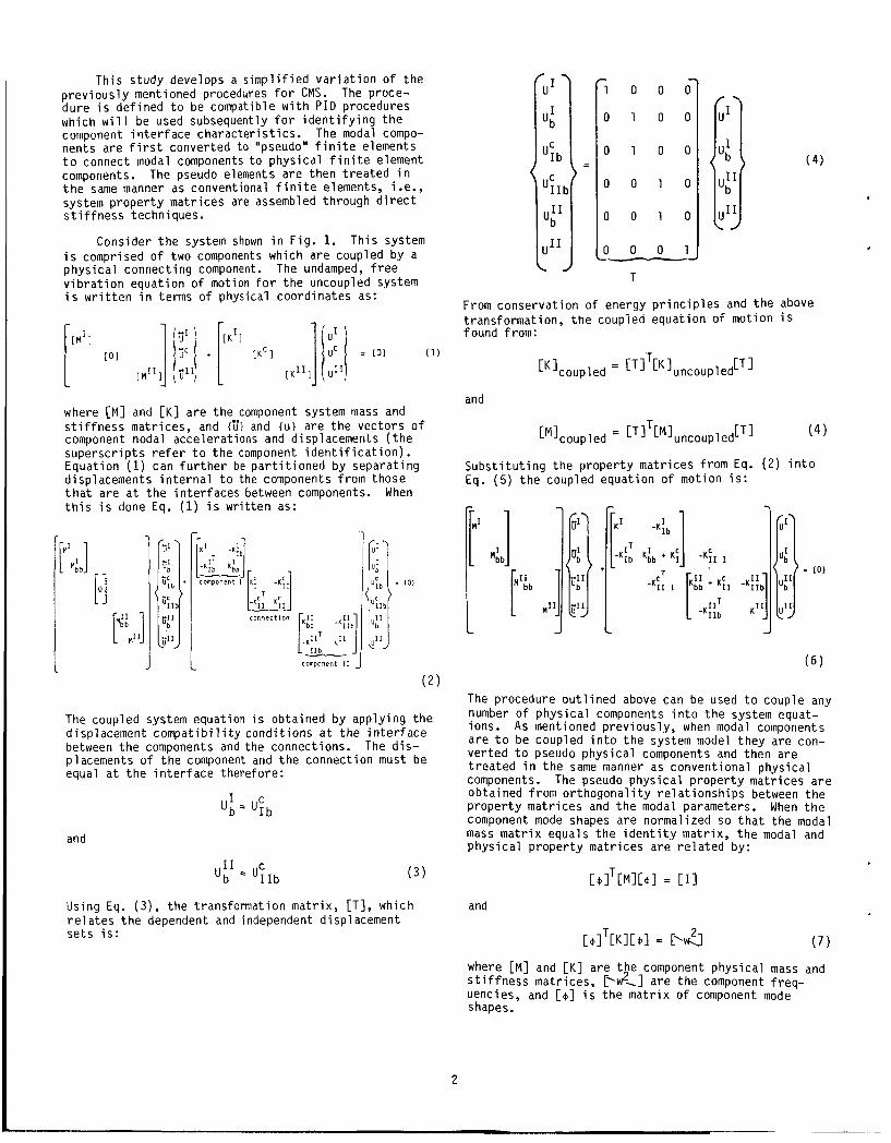
i s comprised o f two components which a re coupled by a p h y s i c a l connect ing component. The undamped, f r e e v i b r a t i o n equat ion o f motion f o r t h e uncoupled system i s w r i t t e n i n terms o f physical coord inates as:

The pseudo elements are then t r e a t e d i n

Consider t h e system shown i n F ig . 1. T h i s system

where [ M I and [ K ] a re t h e component system mass and s t i f f n e s s matr ices, and {:I and {u) are t h e vec to rs of component nodal accelerat ions and displacements ( t h e supersc r ip t s r e f e r t o t h e component i d e n t i f i c a t i o n ) . Equat ion (1) can f u r t h e r be p a r t i t i o n e d by separat ing displacements i n t e r n a l t o the components f rom those t h a t are a t t h e i n t e r f a c e s between components. When t h i s i s done Eq. (1) i s w r i t t e n as:

- (01

component I I J J I ( 2

The coupled system equation i s obta ined by app ly ing t h e d isplacement compat i b i 1 i t y cond i t i ons a t t h e i n t e r f a c e between t h e components and the connections. placements o f t h e component and t h e connect ion must be equal a t t h e i n t e r f a c e therefore:

The d i s -

I C 'b = ' I b

and

( 3 ) I 1

'b = ' i I b

Using Eq. ( 3 ) , t h e t ransformat ion ma t r i x , [TI, which r e l a t e s t h e dependent and independent displacement se ts i s :

"' I - 1 0 0 0

0 1 0 0

0 1 0 0

0 0 1 0

0 0 1 0

0 0 0 1 - T

( 4 )

From conserva t i on o f energy p r i n c i p l e s and t h e above t ransformat ion, t h e coupied equat ion o f moi fu i l i s found from:

[T 1 T [K1coupled = uncoupl ed

and

[T 1 (4) T [M1coupled = [M1uncoupled

S u b s t i t u t i n g t h e p r o p e r t y ma t r i ces f rom Eq. ( 2 ) i n t o Eq. (5 ) t h e coupled equat ion o f mot ion i s :

The procedure o u t l i n e d above can be used t o couple any number of p h y s i c a l components i n t o t h e system equat- ions. As mentioned p rev ious l y , when modal components a r e t o be coupled i n t o t h e system model t h e y a re con- ve r ted t o pseudo p h y s i c a l components and then are t r e a t e d i n t h e same manner as convent ional phys i ca l components. The pseudo p h y s i c a l p r o p e r t y ma t r i ces a r e obta ined f rom o r t h o g o n a l i t y r e l a t i o n s h i p s between t h e p r o p e r t y ma t r i ces and t h e modal parameters. When t h e component mode shapes a re normalized so t h a t t h e modal mass m a t r i x equals t h e i d e n t i t y ma t r i x , t h e modal and p h y s i c a l p r o p e r t y ma t r i ces a re r e l a t e d by:

and

[ t J I T C K l [ o l = [ 4 J ( 7 )

where [ M I and [K ] a re t h e component p h y s i c a l mass and s t i f f n e s s matr ices, [\w?.] a re t h e component f req - uencies, and [ @ ] i s t h e m a t r i x o f component mode shapes.

2

When experimental modal data is used to charac- terize the component, the matrix [$I, containing the component mode shapes may be rectangular. shapes are measured, and the value of the mode shapes are recorded at "n" different physical locations on the component, then the mode shape matrix will be of order n x m. Normally, there will be more measure- ment locations available than there will be modes that can be measured. To obtain a square modal matrix from experimental mode shape data, data at some measurement points can be neglected so that the number of points is equal to the number of modes. ment points is discarded no information is lost as far . as the overall system response is concerned, so long as measurements at the component's interface points are retained. available, the pseudo physical property matrices are related to the modal data by:

If "m" mode

When data at measure-

Once a square mode shape matrix is

and

where [Mp] and [Kp] are the component pseudo mass and stiffness matrices. stiffness matrices are in terms of physical coordinates corresponding to the location and direction where the mode shapes are measured).

pseudo matrices because their physicai interpretation is unlike that of conventional mass and stiffness matrices. Because it is impractical to measure all o f the component modes, the modal data will be incomplete (see (2)) and will not contain all the information required to produce the actual component mass and stiffness matrices. Therefore, although the mass and stiffness matrices computed in Eq. (8) are in terms o f physical rather than modal coordinates, the matri- ces will not necessarily represent the actual physical mass and stiffness characteristics of the component. The mass and stiffness matrices from Eq. (8) will reproduce the measured frequencies and mode shapes, and will be suitable for representing the component in the coupled system model.

nent modes can be used for the component character- ization. correspond to the component when it is in the uncon- strained or free boundary condition. In many situ- ations these modes are more conveniently obtained than the fixed boundary modes. This is particularly true when the modes are measured experimentally, because the component itself does not have to be phys- ically constrained during the experimental testing. In practice, the free boundary condition often is approximated by suspending the component from flexible cords or by supporting it on soft springs.

constraining all of the component's boundary degrees o f freedom while performing the modal testing. Ana- lytically, the fixed modes are computed as easily

(The coefficients of the mass and

The matrices computed in Eq. (8) are designated as

Either the "free" or the "fixed" boundary compo-

The "free" mode shapes are those modes that

The fixed modes are obtained by simultaneously

as the free modes. Experimentally, they are more dif- ficult to obtain, because all of the component's boundary degrees of freedom must be fully constrained during the experiment. To attain this condition requires that elaborate fixtures be attached at the components boundary locations, and in practice, full constraint is never completely achieved. Another dif- ficulty of using fixed boundxy mode shapes is that an additional set of "static" deflection or constraint modes must be added to the set of fixed boundary modes. These modes are required so that the component will have flexibility at its boundary locations where it is connected to adjacent components.

shapes are measured in the translational directions. It is not generally practical to measure the values of the mode shapes in the rotational directions because of limitations in available instrumentation. However, it is sometimes desirable to couple rotational degrees o f freedom between components. mode shapes are not measured in the rotational direc- tions, the pseudo matrices will only have transla- tional degrees of freedom and there will not be means of coupling the rotational connecting stiffnesses. circumvent this difficulty, the rotational values of the mode shapes can be extrapolated from the transla- tional values, either by curve fitting through the translational degrees of freedom and then computing the slope of the curve at the connection location, or by usin an approximate F.E. model of the component (see [d.

Normally, the values of the experimental mode

If the values of the

To

When the rotational values are extrapolated from a curve fit any existing rotttional inertia effects will not be reflected in the values of the rotations. Neglecting the actual independent motion o f the rota- tion implies that there is no rotational inertia and that the rotations are dependent on the translations. Because of this dependence, the combined translational/ rotational mode shapes can not be used directly to compute the pseudo matrices without encountering numer- ical problems during the matrix inversions in Eq. (8). A solution to this difficulty is to initially use only the translational mode shapes to compute the pseudo matrices. Then, a transformation which is based on the dependence between the rotations and translations is used to transform the pseudo matrices from the translational coordinate system to a com- bined translational/rotational system.

shapes can be related to the independent translations by :

The dependent rotational values of the mode

n

(9)

Where U, is the dependent rotation at j , Ubi are

the translations at the independent measurement points, ai translations to the dependent rotations (determined from curve fit, etc.), and n is the number of independent measurement points.

The transformation from the mixed coordinate matrices to the entirely translational pseudo property matrices is:

j

are the coefficients relating the independent

3

where [ T I ] i s the transformation matrix derived from the relationships in Eq. ( 9 ) and { u l ' i s a subset of { u 1 . For each rotational degree o# freedom tha t i s adaed in { u e l , a translational degree of freedom i s removed from { u A ) ' . l a t i ona l degrees of freedom that a re removed i s arbi- t r a ry , and since a translation i s removed f o r each ro ta t ion tha t i s added, both systems will contain the same number of degrees of freedom.

Using the original translational pseudo property matrices from E q . ( 8 ) , the transformation in Eq. ( l o ) ,

matrices are derived in the combined t rans la t iona l / ro ta t iona l coordinate system by:

The selection o f t he trans-

drid principle5 o f conse rva t i on u i oiieryy, L ' - - L l l e pseudo

(111

Once the component pseudo matrices in E q . (11) are computed, they can be inserted into the system equa- t i ons of motion and coupled t o adjacent components using the previously discussed procedures.

t o predict t he overall system dynamic charac te r i s t ics . The frequencies tha t are computed from t h i s equation wi l l correspond t o the overall system resonances. The accuracy of the predicted frequencies will be depend- en t on t he precision with which the connections between components have been modeled. I t has been assumed t h a t t he component modal models have been verified and are accurate, and also, that the proper component modes have been included in the model t o adequately predict system response (see sample problem one).

will correspond t o the physical degrees of freedom included in the system model. translational/rotational model i s used some of the mode shape values will correspond t o t rans la t iona l degrees of freedom and some t o rotations. racy of the mode shapes, l ike the frequencies, will be dependent on the adequacy of the component modal representations and the modeling of the connections.

- Parameter Identification Procedure Once the system equations of motion and t h e i r

corresponding frequencies and mode shapes a re computed, and the experimental system modes have been measured, PI0 can be used t o find an improved s e t of connection parameters t ha t be t te r predict the measured experimen- t a l system data. For t h i s study the Weighted Least Squares method f o r parameter estimation i s used ( 6 ) .

I f { E l and {c ) are vectors containing the measured and computed system frequencies and mode shapes respec- t i ve ly , then the weighted squared difference between t h e predicted and measured charac te r i s t ics i s :

The f ina l coupled system equations can be used

The mode shapes derived f rom the system equations

When the combined

The accu-

where [ W ] i s the weighting matrix and { F > i s a vector of weighted squared differenczs. connection parameters t ha t minimizes the weighted squared differences, the derivative o f I F ) with respect t o the connection parameters i s s e t t o zero. t ha t the predicted charac te r i s t ics { c l , are a f U n C - t ion of t he connection parameters I r l , t he deriva- t i v e of { F I i s written as:

To f ind the s e t of

Noting

Expanding {c ) in a Taylor s e r i e s and truncating higher order terms, {c} i s approximated as:

where t ArJ are the differences between t i l e estiiilaied and actual values f o r the connection parameters. Substi tuting E q . (14) in to E q . ( 1 3 ) and l e t t i ng alc)/a{r}=[S] leads t o :

[W](IC) - I C > e s t - [ S ] I A ~ } ) [ S ] = IO} ( 1 5 )

From Eq. (15) i t i s desired t o solve f o r {Arl so tha t the actual connection parameters can be determined. Solving f o r {At-} can not be iecomplished by simple inversions, however, because in general the number of measured and predicted cha rac t e r i s t i c s will be grea te r than the number of connection parameters, rendering the matrix [SI t o be nonsquare. be olved f o r i f E q . (15) i s f i r s t premultiplied by [S I . When t h i s i s done, { e r ) i s solved as:

The vector {Arl can

il

{At-) = ([s]T[w][s]) -' [slT[W1 ( - {c)EST) (16)

A n updated s e t of connection parameters i s computed by:

I r l = {'IEST + l e r l ( 1 7 )

or by subs t i tu t ing from E q . (16) :

t r} = t r l E S T + ([SI~[WICSI)-'[SI~[WI(~~~ - ICIEST)

(18) Since {c ) i s approximated by a truncated se r i e s ,

the improved connection parameters will be only an approximation t o the f ina l parameters. f i n a l parameters can be obtained by i t e r a t ing on E q . (18).

A d i r e c t approach f o r computing the elements of the sens i t i v i ty matrix [SI i s t o perturb the analyti- ca l model with changes in the connection parameters, and then compute the resu l t ing changes in the system charac te r i s t ics . The elements are then computed by se t t ing T i j equal t o the change in the c i charac- t e r i s t i c divided by the change in the r j connection parameter. Alternative methods f o r computing these der iva t ives have been presented ( see (7)) b u t f o r problems such as the example, with only a small number of connection parameters, the above method i s adequate.

However, the

The selection of the system charac te r i s t ics t h a t a r e used in the estimation procedure i s determined by data acquistion capabili ty. generally eas ie r t o measure frequencies than mode shapes, so in many cases i t may be practical t o include more frequencies t h a n modes shapes.

Experimentally, i t i s

Characterist ics

4

For t h e i n i t i a l a t tempt a t i d e n t i f y i n g t h e con- o t h e r than f requencies and mode shapes a l so can be n e c t i o n p roper t i es , o n l y t h e s imulated system frequen- u t i l i z e d ; i n (81, i t i s suggested t h a t k i n e t i c energy cies from the F.E. model (Table 11) were used in t h e may be a usefuT c h a r a c t e r i s t i c . Once t h e cha rac te r i s - parameter identification routines. It is preferable

t h a t t h e connect ion p r o p e r t i e s be i d e n t i f i e d w i t h o u t t i c s a re chosen, t h e weight t h a t i s placed on each c h a r a c t e r i s t i c must be determined. If one character- having to use system mode shapes because the mode i s t i c i s measured more accu ra te l y than another, then

shapes a re cons ide rab ly more d i f f i c u l t t o experimen- i t can be weighted more heav i l y . t a l l y measure than t h e f requencies. When e i t h e r s i x

When t h e number o f system c h a r a c t e r i s t i c s i s large, t h e s i z e o f t h e we igh t i ng and s e n s i t i v i t y mat- r i c e s increases, and t h e m a t r i x i n Eq. (18) may become ill cond i t i oned f o r i n v e r s i o n (see (2)). procedure o n l y r e q u i r e s a minimum number o f system c h a r a c t e r i s t i c s t o adequately i d e n t i f y t h e connection parameters s i n c e each component has a l ready been ve r i - f i e d . Therefore, t h e s i z e o f t h e ma t r i ces i n Eq. (18) w i l l be kep t smal l and i n v e r s i o n problems w i l l be min- imized. Another problem may a r i s e when t h e a n a l y t i c a l model cannot be e x a c t l y made t o f i t t h e experimental data. When t h i s i s t h e s i t u a t i o n t h e s e t o f connec- t i o n p y a m e t e r s t h a t minimizes t h e d i f f e rences , r a t h e r than e l i m i n a t e s them, must be used. The model may not be ab le t o produce t h e des i red measured system charac- t e r i s t i c s because o f l i m i t a t i o n s i n t h e component modal rep resen ta t i on . Also, i f t h e exper imen ta l l y measured modes a re n o t orthocjanal, p e r f e c t agreement can never be achieved because t h e a n a l y t i c a l model can o n l y produce or thogonal mode shapes.

The P I D

Sample Problem One: Coupled Beams The f o l l o w i n q sample problem i s o f f e r r e d t o dem-

o n s t r a t e t h e component'coupling and parameter i d e n t i - f i c a t i o n procedures. To v e r i f y these procedures s imulated experimental da ta generated from a F.E. model was used. The sample problem (F ig . 2) i s com- p r i s e d o f two s imply supported beams connected a t t h e i r ends. F o r s i m p l i c i t y , bo th beam components were made i d e n t i c a l . I n ac tua l a p p l i c a t i o n s t h e sys- tem can be p a r t i t i o n e d i n t o any s e t o f components t h a t i s des i red. problem a re d i s c r e t i z e d i n t o seven massless, p lana r beam elements. Concentrated t r a n s l a t i o n a l masses are added between t h e elements a t nodes 2 through 7 and 10 through 15. r o t a t i o n a l s p r i n g (K = 10.E5) a t nodes e i g h t and nine. A connect ion a l s o i s made t o ground by a r o t a t i o n a l s p r i n g (K = 10.E5) added t o t h e second component a t node 16.

Each o f t h e components i n t h i s

The components a re connected by a

The accuracy o f t h e computed system frequencies as a f u n c t i o n o f t h e number o f modes used f o r t h e com- ponent rep resen ta t i ons was evaluated w i t h s i x , f ou r , and two component modes (see Table I ) . Both t h e s i x and fou r component mode rep resen ta t i ons produced sys- tem f requenc ies t h a t are i n good agreement w i t h t h e base l i ne F.E. s o l u t i o n . Although t h e r e are o n l y s i x component modes i n t h e F.E. so lu t i on , t h e s i x mode r e p r e s e n t a t i o n does n o t produce exact f requencies because t h e F.E. model has more than 6 degrees of freedom. f i r s t and t h i r d modal frequencies t o be p r e d i c t e d sat- i s f a c t o r i l y b u t does n o t p rov ide enough in fo rma t ion f o r an accurate p r e d i c t i o n o f t h e second and f o u r t h frequencies. so t h a t t h e r e w i l l be a r o t a t i o n a l deqree o f freedom

The two mode rep resen ta t i on a l lows f o r the

A t l e a s t two component modes are requ i red

o r f b u r component mode rep resen ta t i ons were used two p o s s i b l e s o l u t i o n s were found f o r t h e K1 and K2 con- n e c t i n g s t i f f n e s s e s which s a t i s f i e d t h e system f r e - quency c o n s t r a i n t s (see Table 11). was dependent on t h e i n i t i a l s t a r t i n g est imates f o r K1 and K2. Although n e i t h e r s o l u t i o n i s equal t o t h e a c t u a l connect ing s t i f f n e s s e s , t h e f i r s t one i s rea- sonably c l o s e cons ide r ing t h e l i m i t e d number o f system d a t a used and t h e approximation o f t h e component modal rep resen ta t i on . i n p u t i n t o t h e F.E. model t h e y produce system frequen- c i e s t h a t a re ve ry c lose t o t h e exact f requencies. The f i r s t s o l u t i o n does produce a b e t t e r s e t o f system mode shapes. I n an ac tua l app l i ca t i on , w i t h o u t more t h a n system frequency informcit ion, i t would be impos- s i b l e t o determine which o f t h e two s o l u t i o n s i s c l o s e r t o t h e ac tua l values o f t h e connecting s t i f f - nesses. Furthermore, s ince bo th t h e f i v e and two system frequency cases produced s i m i l a r s o l u t i o n s t h e r e i s no advantage t o us ing more than two system f requencies. When two component modes a re used a maximum o f f o u r system f requencies are ava i l ab le , t h e r e f o r e t h e f i v e system frequency case cannot be analyzed. Fo r t h e two component modes and two system f requency case, t h e s o l u t i o n f a i l e d t o converge.

A subsequent attempt, us ing a combination of b o t h system f requencies and made shapes was made w i t h t h e expec ta t i on t h a t t h e i d e n t i f i c a t i o n o f t h e connec- t i o n p r o p e r t i e s would be improved. By adding t h e f i r s t mode shape as a c o n s t r a i n t , along w i t h t h e f i r s t f i v e system frequencies, t h e second m u l t i p l e s o l u t i o n was e l im ina ted . one mode shape was used, t h e problem s t i l l converged t o t h e f i r s t s o l u t i o n rega rd less o f t h e i n i t i a l e s t i - mates f o r t h e connecting s t i f f n e s s e s . o f system da ta i s i d e a l because, w h i l e i t e l i m i n a t e s t h e m u l t i p l e so lu t i on , i t o n l y r e q u i r e s a minimal amount o f experimental data. S i m i l a r r e s u l t s were produced f o r bo th the s i x and f o u r component mode representat ions, w h i l e t h e two mode rep resen ta t i on cont inued t o present d i f f i c u l t i e s .

Sample Problem Two: Once t h e component coup l i ng and parameter i d e n t i -

f i c a t i o n a lgo r i t hms were evaluated w i t h s imulated d a t a (Sample Problem One), i t was decided t o assess t h e procedures us ing ac tua l experimental data. To accom- p l i s h t h i s , t h e RSD (Ro ta t i ng S t r u c t u r a l Dynamics R i g ) a t NASA Lewis Research Center was se lected. The RSD r i g (F ig . 3) i s designed t o s imu la te engine s t r u c t u r e s t o s tudy a c t i v e r o t o r c o n t r o l and system dynamics (component i n t e r a c t i o n ) problems. The r i g components, a l though considerably s imp le r t han a r e a l t u r b i n e engine's, were scaled such t h a t t h e y would s imu la te an ac tua l engine 's s t r u c t u r a l dynamics response c h a r a c t e r i s t i c s .

The chosen s o l u t i o n

When e i t h e r o f t h e s o l u t i o n s are

When o n l y one system frequency and

T h i s combination

RSD R i g V e r i f i c a t i o n

The o b j e c t i v e o f t h e parameter i d e n t i f i c a t i o n was t o determine t h e s t i f f n e s s e s o f t h e s q u i r r e l cage bear- i n g support t h a t connects each end o f t h e r o t o r t o t h e support frame. To accomplish t h i s , t h e RSD r i g was d i v i d e d i n two components; t h e r o t o r suppor t frame, and t h e r o t o r . Each o f these components was charac- t e r i z e d v e r i f i e d exper imenta l ly , so t h a t accurate component rep resen ta t i ons would be a v a i l a b l e f o r t h e

a t each end o f t h e component t h a t i s connected t o ground ( o n l y one mode i s needed f o r t h e o the r compo- nen t ) . I n eve ry case t h e component mode s o l u t i o n produced f requenc ies t h a t are h ighe r than t h e basel ine frequencies. T h i s i s understandable s ince t h e compo- nent mode s o l u t i o n uses a t runca ted s e t o f modes and t h e r e f o r e does n o t i nc lude a l l of t h e component's f l e x i b i l i t y .

5

coupled system model. I n the system model t h e support frame was represented by an exper imenta l ly v e r i f i e d F.E. model w h i l e t h e r o t o r component was represented by experimental modal data. Since b o t h components were exper imen ta l l y v e r i f i e d , any d i f f e r e n c e s t h a t appeared between t h e p r e d i c t e d and measured system charac te r i s - t i c s cou ld be a t t r i b u t e d t o the u n c e r t a i n t i e s i n t h e s q u i r r e l cage connections between components. T h i s approach cons ide rab ly s i m p l i f i e d t h e v e r i f i c a t i o n t a s k by reducing t h e q u a n t i t y of modal da ta requ i red f r o m t h e coupled system.

F ig. 4. p l a t e so g r i d p o i n t s 35 through 39 are f u l l y const ra ined. G r i d p o i n t s 19 and 20, where t h e r o t o r i s attached, were al lowed t o f r e e l y displace. i s r e p r e s e n t a t i v e o f t h e cond i t i ons used d u r i n g t h e modal t e s t s and i s a l s o compatibie w i t h t n e requ i re - ments f o r t h e component coupl ing procedure. The g r i d p o i n t s a re connected wi th beam (bending and a x i a l deformat ions) elements except f o r t h e diagonal elements a t g r i d 35 which are modeled w i t h r o d ( a x i a l deforma- t i o n o n l y ) elements. A l l o f t h e elements a re modeled w i t h A36 s t e e l p r o p e r t i e s . The frame F.E. model was analyzed w i t h NASTRAN, t o compute t h e component f r e - quencies and mode shapes ( F i g . 5 ) . were exper imen ta l l y v e r i f i e d by us ing v i b r a t i o n d a t a obta ined f rom an HP 5423 Dynamic Analyzer. modal rep resen ta t i on was obtained by measuring t h e r o t o r mode shapes i n t h e f r e e boundary cond i t i on . c o n d i t i o n was approximated by hanging t h e r o t o r f rom bungy cords. The component modal c h a r a c t e r i s t i c s were generated f rom t r a n s f e r f u n c t i o n da ta obta ined f rom t h e dynamic analyzer and impact t e s t i n g . A t o t a l o f s i x r o t o r modes were measured (see F ig. 6 ) i n c l u d i n g two r i g i d body and f o u r e l a s t i c modes.

b i n i n g t h e phys i ca l F.E. model o f t h e frame w i t h t h e modal rep resen ta t i on o f t h e r o t o r . For s i m p l i c i t y t h e coupled system model was const ra ined t o mot ion o n l y i n t h e v e r t i c a l plane. T h i s r e s t r i c t i o n al lowed f o r a r e d u c t i o n i n t h e r e q u i r e d number o f degrees o f freedom i n t h e system model and allowed f o r a l l o f t h e system t e s t i n g t o be performed i n one plane. The coupled sys- tem f requencies f o r t h e s i x mode r o t o r rep resen ta t i on a r e p l o t t e d along w i t h t h e measured f requencies i n F ig . 7. The p r e d i c t e d frequencies were computed f o r d i f f e r e n t values o f s q u i r r e l cage s t i f f n e s s t o deter- mine t h e e f f e c t t h a t t h e cages have on t h e system f r e - quencies. To generate these r e s u l t s i t was assumed t h a t b o t h s q u i r r e l cages had i d e n t i c a l s t i f f n e s s e s . Th is was a r a t i o n a l assumption, since bo th cages a r e b u i l t t o t h e same s p e c i f i c a t i o n s . cage s t i f f n e s s was measured as 5050 l b / i n . us ing a s t a t i c l oad ing t e s t . )

The suppor t frame f i n i t e element mesh i s shown i n The frame i s mounted on a r e l a t i v e l y s t i f f base

T h i s f r e e c o n d i t i o n

The f requencies

The r o t o r

Th is

The suppor t frame and r o t o r were coupled by com-

(Subsequent t o t h i s ana lys i s t h e

Only t h e f i r s t t h r e e computed system f requencies a re shown because o n l y th ree f requencies were measured. When a l l t h r e e f requencies a re used t h e cage s t i f f n e s s i s i d e n t i f i e d as 5750 l b / i n . agreement w i t h t h e measured s t i f f n e s s (5050), consider- i n g t h a t o n l y t h r e e system f requencies were used f o r t h e parameter i d e n t i f i c a t i o n . I n F ig . 7 i t i s shown t h a t t h i s amount o f d i f f e r e n c e i n cage s t i f f n e s s does n o t have a s i g n i f i c a n t e f f e c t on t h e system f requencies

T h i s va lue i s i n good

I n a d d i t i o n t o t h e s i x mode r o t o r representat ion, a f o u r and two mode rep resen ta t i on were used t o deter- mine t h e e f f e c t t h a t t h e number o f component modes has on t h e s t i f f n e s s i d e n t i f i c a t i o n . The f o u r mode repre- s e n t a t i o n i d e n t i f i e d t h e same cage s t i f f n e s s as t h e s i x

mode rep resen ta t i on . t i f i e d t h e cage s t i f f n e s s as about 2300 l b / i n . o r o n l y 46 pe rcen t of t h e measured s t i f f n e s s . It was expected t h a t t h e two mode rep resen ta t i on would be i n s u f f i c i e n t f o r i d e n t i f y i n g t h e cage s t i f f n e s s because t h i s repre- s e n t a t i o n i s inadequate f o r accu ra te l y p r e d i c t i n g t h e system modes. I t i s obvious t h a t t h e two mode repre- s e n t a t i o n cannot produce very good r e s u l t s because o n l y r i g i d body modes a re i nc luded i n t h e representa- t i o n , and t h e system modes i n v o l v e e l a s t i c bending i n t h e r o t o r . Although r u l e s o f thumb a re a v a i l a b l e f o r determin ing t h e r e q u i r e d number o f modes, a d d i t i o n a l work i s r e q u i r e d i n t h i s area.

The two mode rep resen ta t i on iden-

CONCLUSION

From t h e two sample problems analyzed i n t h i s s tudy i t was determined t h a t t h e s t i f f n e s s c h a r a c t e r i s t i c s of Luiiipurierit iuiinectiori~ caii be i d e f i t i f j e d i i s i i i g component mode syn thes i s and parameter i d e n t i f i c a t i o n procedures. Furthermore, t h e c h a r a c t e r i s t i c s can be i d e n t i f i e d us ing exper imen ta l l y obta ined component modal r e p r e s e n t a t i o n and a minimal q u a n t i t y o f measured system modal data. I n t h e f i r s t sample problem i t was found t h a t m u l t i p l e s o l u t i o n s are poss ib le , bu t t h a t t h e y can be avoided when system mode shapes are i nc luded i n t h e i d e n t i f i - c a t i o n procedure. I n t h e second problem i t was found t h a t t h e r o t o r f o r a r o t o r l s u p p o r t frame coupled sys- tem cou ld be adequately represented by exper imen ta l l y obta ined modal data. I t was a l s o found t h a t o n l y t h r e e system f requencies had t o be measured f o r t h e connec- t i o n c h a r a c t e r i s t i c s between t h e frame and r o t o r t o b e i d e n t i f i e d . From t h e r e s u l t s obta ined thus f a r , i t i s determined t h a t t h e q u a n t i t y o f da ta r e q u i r e d f o r t h e component rep resen ta t i ons and f o r t h e connect ion char- a c t e r i s t i c i d e n t i f i c a t i o n i s problem dependent. There- fo re , each a p p l i c a t i o n must be t r e a t e d on an i n d i v i d u a l bas is .

REFERENCES

1. Hurty, W.C., 1964, "Dynamic Ana lys i s o f S t r u c t u r a l Systems by Component Mode Synthesis," JPL-TR-32-350,

NASA CR-53057.

2. Craig, R.R. Jr., 1981, S t r u c t u r a l Dynamics, John Wi ley and Sons, New York.

3. Mart inez, D.R., and Gregory, D.L., 1984, "A Com- p a r i s o n o f Free Component Mode Synthes is Tech- n iques Using MSCINASTRAN," SAND 83-0025.

4. Berman, A., and F lanne l l y , W.G., 1971, "Theory o f Incomplete Models of Dynamic St ructures," AIAA Journal Vol. 9, No. E, pp. 1481-1487.

5. Berman, A . , and Nagy, E.J., 1982, Improvement o f a Large Dynamic A n a l y t i c a l Model Using Ground V i b r a t i o n Test Data," A I A A 23rd Structures, St ruc- t u r a l Dynamics and M a t e r i a l s Conference, P a r t 1, A I A A , New York, pp. 301-306.

6. Isenberg, J. , 1979, "Progress ing from Least Squares i n Bayesian Estimation," ASME Paper 79-WA/DSC-16.

7. C o l l i n s , J.D., Hart, G.C., Hasselman, T.K., and Kennedy, E., 1974, " S t a t i s t i c a l I d e n t i f i c a t i o n of St ructures," A I A A Journal, Vol. 12, No. 2,

-3

PP. 185-190.

6

, Wada, B.K., Garba, J.A., and Chen, J.C., 1983, Modal Test and Ana lys i s Cor re la t i on , " Modal T e s t i n g and Model Refinement, AMD-Vo1.rD.F.H. Chu, ed., ASME, New York, pp. 85-99.

425

523

932

9. Hasselman, T.K., 1983, "A Pe rspec t i ve on Dynamic Model V e r i f i c a t i o n , ' ' Modal Tes t i ng and Model Refinement, AMD-Vol. 59, D.F.H. Chu, ed., ASME, New York, pp. 101-117.

+9

t 1

t 1

7 . 1 7 ~ 1 0 6 426

1.09x107 525

3 . 4 4 ~ 1 0 ~ 933

Base 1 i n e f i n l t e - e lement so 1 u t i o n ,

H Z

1.94~105. (112)

.07x106 (165)

1 . 9 9 ~ 1 0 6 (421)

1.12x106 (496)

1 . 3 9 ~ 1 0 ~ (927)

. igenva 1 ue t p e r c e n t

5 . 1 1 ~ 1 0 ~ t2

1 . 2 3 ~ 1 0 ~ * l

1 . 13X1O6 t1

1 .OBx1O7 t l

3 . 4 3 ~ 1 0 '

TABLE 11. - COHPUlEO CONNECTION STIFkNESS

Component mode s y n t h e s i s s o l u t i o n

E igenva lue Frequency, Freq:zncy* I + p e r c e n t 1 Hz

114 5 . 1 2 ~ 1 0 ~ 114

111 I 1.2;:lOb I 180

E i g e n v a l u e + p e r c e n t

5 . 2 5 ~ 1 0 5 t3

1 . 5 1 ~ 1 0 5 +21

7 . 5 4 ~ 1 0 6 t 4

1 . 1 2 ~ 1 0 7

Frequency,

Number of Number o f component modes system

f r e q u e n c l e s

Connect ion s t i f f n e s s

3 . 1 ~ 1 0 5 1 3 . 1 ~ 1 0 5 3 . 6 ~ 1 0 5 1 2 . 5 ~ 1 0 5

6 . 1 ~ 1 0 ~ 1 . 4 ~ 1 0 ~ 4 . 1 ~ 1 0 ~ 1 0 . 8 ~ 1 0 ~

3 . 7 ~ 1 0 5 1 3 . 4 ~ 1 0 5 5 . 4 ~ 1 0 5 8 . 1 ~ 1 0 5

aOnly ( o u r system f r e q u e n c l e s a v a i l a b l e b s o l u t l o n doer n o t converge.

P = 1 . 0

I = 1 . 0 AL = 1 . 0

E = 1x105

K1 = K 2 = 1oX105 K1

I

11 \ L J l " I . u,

FIGURE 1 . - THREE CWONENT SYSTEM.

16

FIGURE 2.- COUPLED SYSTEM (SAWLE PROBLEM ONE).

7

8

1

16

8

16

14 30

36

5

27

39

FIGURE 4 . - SUPPORT FRAME F.E. MODEL.

9

MODE 1: 35 Hz RODE 2: 41 Hz

MODE 3: 61 Hz RODE 4: 72 Hz

RODE 5 : 80 Hz

FIGURE 5.- SUPPORT FRAME RODE SHAPES.

10

MODE 1: 0 Hz

MODE 2: 0 Hz

MODE 3: 141 Hz

MODE 4 : 304 Hz

MODE 5: 609 Hz

MODE 6: 897 Hz FIGURE 6 . - ROTOR HODE SHAPES.

11

MEASURED SYSTEM FREQUENCIES PREDICTED SYSTEM FREQUENCIES

MODE 3 N I

60 V L

MODE 1

30

20 1000 2500 3750 5050 10 000

SQUIRREL CAGE STIFFNESS, LB/IN.

FIGURE 7.- COUPLED FRAME/ROTOR ANALYSIS ( 6 COMPONENT MODES).

12

1. Report No. NASA TM-88960

I 4. Titie and Subtitle

I d e n t i f i c a t i o n o f S t r u c t u r a l I n t e r f a c e Charac te r i s t i cs Using Component Mode Synthesis

2. Government Accession No. 3. Recipient's Catalog No.

5. Report Date

6. Performing Organization Code

505-63-1 1

7. Author(s)

A.A. Huckelbr idge and C. Lawrence 8. Performing Organization Report No.

E-341 5

10. Work Unit No. r

21. No. of pages 9. Security Classif. (of this report) 20. Security Classif ( f this pa e Unc lass i f i ed Uncj as s i ? ed 13

9. Performing Organization Name and Address

Nat iona l Aeronautics and Space Admin is t ra t ion Lewis Research Center Cleveland, Ohio 44135

22. Price' A02

11. Contract or Grant No.

13. Type of Report and Period Covered

I 2. Sponsoring Agency Name and Address

Nat iona l Aeronautics and Space Admin is t ra t ion Washington, D.C. 20546

Tec h n i c a l Memorandum

14. Sponsoring Agency Code 1 5. Supplementary Notes

Prepared f o r the V ib ra t ions Conference, sponsored by t h e American Society o f Mechanical Engineers, Boston, Massachusetts, September 27-30, 1987. A.A. Huckelbridge, Case Western Reserve Un ive rs i t y , Cleveland, Ohio; C. Lawrence, NASA Lewis Research Center.

6. Abstract

The i n a b i l i t y t o adequately model connections has l i m i t e d the a b i l i t y t o p r e d i c t o v e r a l l system dynamic response. Connections between s t r u c t u r a l components a r e o f t e n mechanically complex and d i f f i c u l t t o accura te ly model a n a l y t i c a l l y . Improved a n a l y t i c a l models f o r connections are needed t o improve system dynamic p red ic t i ons . coup l ing s t r u c t u r a l components w i t h Parameter I d e n t i f i c a t i o n procedures f o r improving the a n a l y t i c a l modeling o f the connections. Improvements i n the con- nec t i on proper t ies a re computed i n terms o f phys i ca l parameters so the phys i ca l c h a r a c t e r i s t i c s o f the connections can be b e t t e r understood, i n a d d i t i o n t o pro- v i d i n g improved inpu t f o r the system model. Two sample problems, one u t i l i z i n g s imulated data, the o ther us ing exper imental data f rom a r o t o r dynamic t e s t r i g a re presented.

This study explores combining Component Mode synthes is methods f o r

7. Key Words (Suggested by Author@))

Parameter i d e n t i f i c a t i o n Component mode synthesis S t r u c t u r a l connections

18. Distribution Statement

Unc lass i f i ed - u n l i m i t e d STAR Category 39

I I I

*For sale by the National Technical Information Service, Springfield, Virginia 221 61