ICT WORKSHOP FOR SCIENCE PGCE February … Studio Set-up texts (Feb...ICT WORKSHOP FOR SCIENCE PGCE...

Insight iLOG Studio – Data-logging workshop (Laurence Rogers) 1

ICT WORKSHOP FOR SCIENCE PGCE February 2012

Group work in pairs or triads

DATA LOGGING

Insight iLOG Studio Welcome Wizard:

Click Experiment set-ups and select files on the

My Documents tab.

Physics lab:

Current & voltage current, voltage

Force & acceleration time

Free fall time

Pendulum motion angle

Radioactive decay GM detector

Runaway car time

Thermal conductivity temperature

Walkabout motion

Chemistry Lab:

Antacid neutralisation pH

Boyle’s Law pressure

Cooling liquid to solid temperature

Evaporation temperature

Microclimate temperature

Rate of reaction light

Why do animals huddle? temperature

Page

2

4

6

8

11

14

16

18

20

22

24

26

28

30

32

Choose one experiment,

perform the worksheet

activity as directed and record

the results.

Analyse the skills needed to

perform the activity.

Write brief notes on the

advantages and disadvantages

to learning for the activity.

Demonstrate your chosen

experiment to another pair of

students, highlighting the

potential benefits to learning.

EVALUATION of an activity

For each activity consider these questions and write down your answers.

What are the intended learning outcomes for knowledge, skill and understanding?

What is the special ‘added’ value of using ICT for this activity? (Identify the special

qualities of the ICT based method compared with equivalent conventional methods.)

Follow-up reading and resources Rogers, L.T. (2005) ICT for Measurement: Data-logging. In: Sang, D & Frost, R.

(Eds.) Teaching Secondary Science using ICT. London: Hodder Murray.

Newton, L.R. & Rogers, L.T. (2003) Thinking Frameworks for Planning ICT in

Science Lessons. School Science Review 84(309) pp.113-120.

ICT for IST Project – Training pack; http://ictforist.oeiizk.waw.pl/

Data-logging software; www.insightresources.co.uk/pgce11

http://ictforist.oeiizk.waw.pl/

http://www.insightresources.co.uk/pgce11


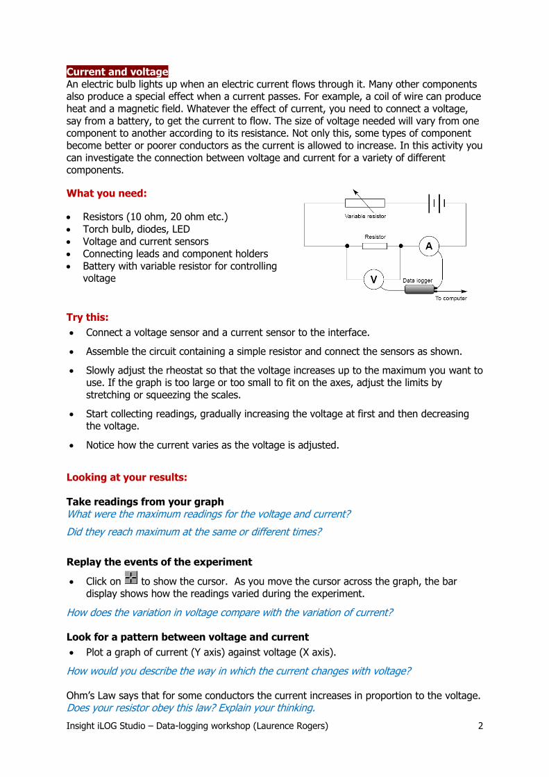
Current and voltage An electric bulb lights up when an electric current flows through it. Many other components also produce a special effect when a current passes. For example, a coil of wire can produce heat and a magnetic field. Whatever the effect of current, you need to connect a voltage, say from a battery, to get the current to flow. The size of voltage needed will vary from one component to another according to its resistance. Not only this, some types of component become better or poorer conductors as the current is allowed to increase. In this activity you can investigate the connection between voltage and current for a variety of different components.

What you need:

Resistors (10 ohm, 20 ohm etc.)

Torch bulb, diodes, LED Voltage and current sensors Connecting leads and component holders Battery with variable resistor for controlling

voltage

Try this:

Connect a voltage sensor and a current sensor to the interface.

Assemble the circuit containing a simple resistor and connect the sensors as shown.

Slowly adjust the rheostat so that the voltage increases up to the maximum you want to use. If the graph is too large or too small to fit on the axes, adjust the limits by stretching or squeezing the scales.

Start collecting readings, gradually increasing the voltage at first and then decreasing the voltage.

Notice how the current varies as the voltage is adjusted.

Looking at your results: Take readings from your graph What were the maximum readings for the voltage and current?

Did they reach maximum at the same or different times?

Replay the events of the experiment

Click on to show the cursor. As you move the cursor across the graph, the bar display shows how the readings varied during the experiment.

How does the variation in voltage compare with the variation of current? Look for a pattern between voltage and current

Plot a graph of current (Y axis) against voltage (X axis).

How would you describe the way in which the current changes with voltage? Ohm’s Law says that for some conductors the current increases in proportion to the voltage. Does your resistor obey this law? Explain your thinking.


More experiments

Comparing two resistors Now do a similar experiment with a different resistor and look out for similarities and differences. If you want to keep the first set of results on the screen, select ‘Overlay’ from the ‘Set up’ menu before you collect another set of results. For further experiments, try combining two similar resistors in series or in parallel. Compare the results and decide what they tell you about how much current flows in each circuit. What conclusions can you draw about the effects of combining resistors? Comparing different components This type of experiment can be used to find out the electrical properties of a range of different components. Try it with a torch bulb and notice how the graph depends upon whether you are increasing or decreasing the voltage. Try also diodes and LEDs for some surprises. Further work Find out about the ‘resistance’

Click on the 'Formula' button and select 'New'.

Type the name Resistance and alter the symbol to ‘R’.

Build the formula 'R = V / I' for the new set of data 'R'. Click OK.

The new graph line 'R' shows the calculations of resistance for each pair of voltage and current readings. How did the resistance vary with the voltage and current?

Repeat this for different resistors and combinations of resistors. What can you learn from comparing the graphs?

Find out about electrical power Components carrying a current convert electrical power. You calculate power by multiplying the voltage by the current. To find out how much power was used in the circuit, create a new set of data as follows:

Click on the 'Formula' button and select 'New'

Type the name ‘Power’ for the new channel and give it the symbol ‘P’.

Build the formula 'P = V * I' for the new set of data 'A'.

Click OK.

The new graph line 'P' shows the calculations of power for each pair of voltage and current readings. How does the power vary with voltage and current?

Investigate the shape of the graph using 'Change' and 'Interval' on the 'Analyse' menu.


Force and acceleration

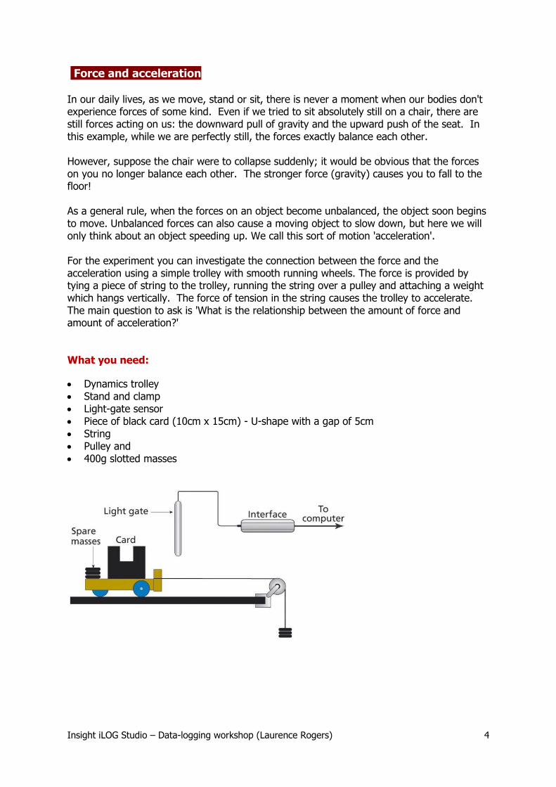
In our daily lives, as we move, stand or sit, there is never a moment when our bodies don't experience forces of some kind. Even if we tried to sit absolutely still on a chair, there are still forces acting on us: the downward pull of gravity and the upward push of the seat. In this example, while we are perfectly still, the forces exactly balance each other. However, suppose the chair were to collapse suddenly; it would be obvious that the forces on you no longer balance each other. The stronger force (gravity) causes you to fall to the floor! As a general rule, when the forces on an object become unbalanced, the object soon begins to move. Unbalanced forces can also cause a moving object to slow down, but here we will only think about an object speeding up. We call this sort of motion 'acceleration'. For the experiment you can investigate the connection between the force and the acceleration using a simple trolley with smooth running wheels. The force is provided by tying a piece of string to the trolley, running the string over a pulley and attaching a weight which hangs vertically. The force of tension in the string causes the trolley to accelerate. The main question to ask is 'What is the relationship between the amount of force and amount of acceleration?' What you need:

Dynamics trolley Stand and clamp Light-gate sensor Piece of black card (10cm x 15cm) - U-shape with a gap of 5cm String Pulley and 400g slotted masses


Preparation

Prepare the card with two accurately cut vertical segments and attach it to the trolley.

Clamp the light-gate sensor so that the card passes through the beam when the trolley moves along the bench.

Clamp the pulley on the edge of the bench, tie one end of the string to the slotted mass holder, run the string over the pulley and attach the other end to trolley.

Try this:

Begin with a falling mass of 100g giving a tension of 1 newton. Place the spare 300g mass on the trolley.

Pull the trolley away from the pulley so that the slotted mass is raised to a point just below the pulley.

Click on START and release the trolley, allowing the mass to fall and the trolley to move along the bench.

Repeat the measurement several times, each time recording the force of 1 newton in the table.

Take one of the 100g masses from the trolley and add it to the falling mass, making the tension force 2 newton. Pull back and release the trolley to make more measurements.

Repeat the process to obtain measurements for 3 and 4 newtons.

Each time you release the trolley, record the string tension in the 'Force' column of the table.

Looking at your results: Look at a bar chart of the results

In the full size Table, click on the heading of the 'Acceleration' column to highlight all

the acceleration values and click on the 'Chart' button .

What does the shape of the chart tell you about the range of results for acceleration?

Look at the graph of acceleration vs. force

Click on to show the cursor. As you move the cursor across the graph, the bar display shows how the acceleration varied during the experiment.

Think about the connection between the acceleration and the force.

Find out what sort of line fits the graph:

Click on the 'Trial fit' button to show the choice of line fitting formulae. Experiment to find out which formula gives the best fit line.

Theory predicts that the acceleration varies in proportion to the applied force. Do your results indicate this?


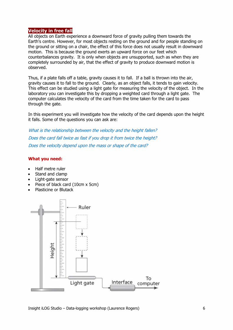
Velocity in free fall All objects on Earth experience a downward force of gravity pulling them towards the Earth's centre. However, for most objects resting on the ground and for people standing on the ground or sitting on a chair, the effect of this force does not usually result in downward motion. This is because the ground exerts an upward force on our feet which counterbalances gravity. It is only when objects are unsupported, such as when they are completely surrounded by air, that the effect of gravity to produce downward motion is observed. Thus, if a plate falls off a table, gravity causes it to fall. If a ball is thrown into the air, gravity causes it to fall to the ground. Clearly, as an object falls, it tends to gain velocity. This effect can be studied using a light gate for measuring the velocity of the object. In the laboratory you can investigate this by dropping a weighted card through a light gate. The computer calculates the velocity of the card from the time taken for the card to pass through the gate. In this experiment you will investigate how the velocity of the card depends upon the height it falls. Some of the questions you can ask are:

What is the relationship between the velocity and the height fallen?

Does the card fall twice as fast if you drop it from twice the height?

Does the velocity depend upon the mass or shape of the card?

What you need:

Half metre ruler Stand and clamp Light-gate sensor Piece of black card (10cm x 5cm) Plasticine or Blutack


Try this:

Assemble the apparatus so that the light-gate sensor is about 20 cm above the bench and the zero mark of the ruler is level with the light-gate.

Prepare the card by drawing a line across the middle and attach a blob of plasticine or Blutack to each lower corner.

Click on START when you are ready to take measurements.

Hold the card so that its mid-point is 10 cm above the sensor. Then release it so that it falls through the light-gate.

Record the height fallen in the 'Height' column of the table.

Drop the card again from the same height and see if the previous result is repeated.

Repeat this process several times, dropping the card from different heights.

Looking at your results: Look at the graph of velocity vs. height

Click on to show the cursor. As you move the cursor across the graph, the bar display shows how the velocity varied during the experiment.

Think about the connection between the velocity and the height fallen.

Find out what sort of line fits the graph

Click on the 'Trial fit' button to show the choice of line fitting formulae. Experiment to find out which formula gives the best fit line. Theory predicts that the velocity varies according to the square root of the height.

Do your results indicate this?

Search for a pattern in the results Test the idea that the velocity varies with the square root of the height like this:

Add a new column to the table and build a formula to calculate the square root of height.

Adjust the horizontal axis to show square root of height.

If you get a straight line, the idea is confirmed. Another test of the connection between velocity and height is to plot velocity squared against height:

Add a new column to the table and build a formula to calculate the square of velocity.

Adjust the axes to show the square of velocity (vertical) against height (horizontal).

If you get a straight line, the pattern is confirmed.


Pendulum motion The pendulum has been used for hundreds of years to help clocks keep time. Many large clocks on churches and town halls still use a pendulum. Some people have a grandfather clock which shows the pendulum swinging inside a tall cabinet, but even small clock such as a cuckoo clock show a pendulum swinging below the clock dial. A pendulum is a simple device. All you need is a weight (the pendulum ‘bob’) suspended on the end of a piece of string, or better still some stiff wire. When you set it swinging, you can measure passing time by counting the number of swings of the bob. You can begin to understand pendulums by using one connected to the computer. Remember that the time for one complete swing of a pendulum, there and back, is called a ‘period’; also, that the size of a swing is called the ‘amplitude’.

The experiment

What you need:

Position/angle sensor 1m of stiff wire supporting a mass of 100g. Stand and clamp

Preparation

Clamp the angle sensor so that it slightly overhangs the bench.

Fix the mass to one end of the stiff wire.

Attach the other end of the wire to the angle sensor so that the bob can swing freely.

Before obtaining measurements, you need to set the scale for the Y axis as follows:

Select ‘Calibration’ from the ‘Setup’ menu. Look at the Signal level gauge and rotate the body of the angle sensor so that the resting position of the pendulum reads about 50%.

Click on the ‘<’ button to define the ‘Low’ signal level, making the physical value ‘0’.


Hold the pendulum at an angle of about 20 degrees to vertical.

Click on the ‘<’ button to define the ‘High’ signal level, making the physical value ‘20’. Then set the axes limits to ‘Upper: 20’ and ‘Lower: -20’ and click on OK.

Try this:

Hold the pendulum to one side so that the angle to vertical is no more than 20.

Start logging and release the pendulum. Notice how the graph records the swings.

When recording stops, wait for a further 10 swings and start logging again. Notice how a new line appears on the graph.

Repeat this to obtain 4 graph lines.

Looking at your results: Replay the events of the experiment

Show just one set of data on the graph.

Click on to show the cursor. As you move the cursor across the graph, the bar display shows the pendulum movements during the experiment.

What points on the graph show the angle of the pendulum at a maximum?

When the pendulum passes through its vertical position, what value for the angle do you expect on the graph?

Now display two sets of data. Notice that one channel shows the pendulum when the swings have died down a little.

Which graph line was recorded first?

Add to the display the other channels. The overlaying graph lines allow you to compare the swings as they die away.

Think about the similarities and differences between the angles as they change. Do the smaller swings last for a shorter time than larger swings?

Does the time for the graph to rise to a peak depend upon the size of swing?

Measure the time of swing

The time between two adjacent peaks is called the ‘period’ of the pendulum.

Display one channel only.

Select ‘Interval’ from the ‘Analyse’ menu and measure the first period.

Make further measurements to find out if the period changes as the swings gradually die away.


Measure the velocity of the pendulum

Display one channel only.

Zoom in to show two peaks and two dips.

The steepness of the line shows the angular velocity of the pendulum. Look at the graph line and predict where the positions of maximum and minimum velocity are.

Check your prediction using the ‘Gradient’ tool on the ‘Analyse’ menu. As you move the cursor, the gradient indicates the velocity at any point.

Plot a graph of velocity You can see how the velocity of the pendulum varies during a complete swing by calculating some new data, as follows:

Display just one channel.

Click the Formula button on the toolbar.

Build a formula which calculates dy/dt for the channel on display.

Describe the similarities and differences between the velocity graph and the angle graph.

Write down a simple rule which describes the connection between the angle and the velocity of the pendulum.


Radioactive decay A special property of a radioactive substance is that it is continually decaying. It gives off invisible radiations which can be detected by a Geiger-Muller counter. The readings give information about the rate of decay and the half life of the substance. In this experiment, radioactive Thorium decays to give Protactinium which can be separated using and organic solvent. The protactinium is also radioactive and its decay can be measured by placing the detector close to the solvent. You will use the computer to record the radiations and measure the ‘half life’ of protactinium. The ‘half life’ of a substance is the time taken for half of the substance to decay.

What you need:

Protactinium source Clamp stand Geiger-Muller detector

Try this:

Connect a radiation detector, such as a Geiger Muller tube, to the interface.

You will use the radioactive substance protactinium in a liquid form in a sealed tube. Place the tube in a vertical position taking care not to mix its contents.

Clamp the detector as close as possible above the tube so that it can record the count rate from the top layer of liquid.

Record the count rate for 5 minutes. Then measure the average count rate using ‘Average’ on the ‘Analyse’ menu and write this down recording it as the ‘background count rate.

When you are ready to start, shake the tube for three seconds and replace it underneath the detector.

Start logging and observe the pattern of results on the graph.



Click on to show the cursor. As you move the cursor across the graph, the bar display shows how the readings varied during the experiment.

How steady were the results during the experiment? Describe the overall trend. Make a smoother graph line Creating a smoother version of the results makes it easier to see the trend.

Select 'Smooth' from the 'Data' menu. In the 'Smooth' dialogue box, select the channel which you want to smooth.

Click on 'Plot' to show the smooth line. If you want a smoother line, click on 'Plot' again.

Does this show the trend in the results any better? Explain why. See if a curve fits your graph

Select 'Zone' from the 'View' menu and click and drag the mouse to draw a Zone box to fit round the points on the graph, omitting the small readings towards the end of the experiment.

Click on the 'Trial fit' button to show the dialogue box:

Click the channel button so that it reads 'Fit to C'.

Click on 'Plot' and each formula in turn to see which give the best fit to the 'C' graph. This is usually an exponential curve.

When you are satisfied with the line, click on 'Store'; the line of best fit data will be stored as a new channel. Find out about the rate of decay Use the curve you have just fitted to your results to study how the rate of decay of the radioactive substance changed during the experiment.

Select ‘Rate’ from the’ Analyse’ menu. Move the cursor so that the vertical line is on a high part of the curve.

Double click the mouse button. This should fix the line at that spot. As you move the cursor a little to the right, the control panel shows how quickly the count rate is reducing.

Repeat this for different starting points on the curve and look for a regular pattern.

What happens to the rate of decay as the experiment proceeds?


Further work Allowing for the background count The detector should be as close as possible to the top of the tube so that it can detect the radiation from the radioactive substance dissolved in the upper layer of liquid. However, some radiation from the lower part of the tube and from the general surroundings is bound to be also picked up by the detector. To correct for this on the graph, you can calculate a new set of data by subtracting the general background value (which you recorded at the very beginning of the experiment) from the results. In the example here, the background count was 5.6.

Click on the 'Formula' button and select 'New'

Type the name ‘Corrected count’ for the new channel.

Build the formula 'A = C - 5.6' for the new set of data 'A'.

Click OK.

The new graph line 'A' shows the calculations for each value of the count rate C. Find the half life of the active substance Use ‘Trial fit’ to plot a smooth curve which shows the underlying trend in the results. Which type of curve best fits the results?

What are the properties of this curve shape?

Use this curve to find the half life of the substance as follows:

Select ‘Ratio’ and ‘Interval’ from the ‘Analyse’ menu. Move the cursor so that the vertical line is on a high part of the curve.

Double click the mouse button. This should fix a line at that spot. As you move the cursor to the right, the ratio between values shows on the control panel.

Adjust the cursor until the ratio shows ‘0.50’. The time interval then gives the half life of the active substance.

Double click to fix a line at a different point on the curve so that you can repeat this again.

What is the half-life? Do you need to take an average of several values?

Why is it better to use the fitted curve than the actual results for finding the half life?


The runaway car ( ((From Insight iLOG Junior – KS3)

The speed of a car (and your mountain bike!) increases as it goes downhill. In this investigation you can use the program to calculate the speed of a model car on a ramp. You can find out how the speed depends on the distance rolled and the angle of the slope.

What you need:

A model car (or several if you want to compare models).

A ramp on which your car can run (about 1m length).

Light gate sensor for timing.

Black card, fixed on the top of the car (see below).

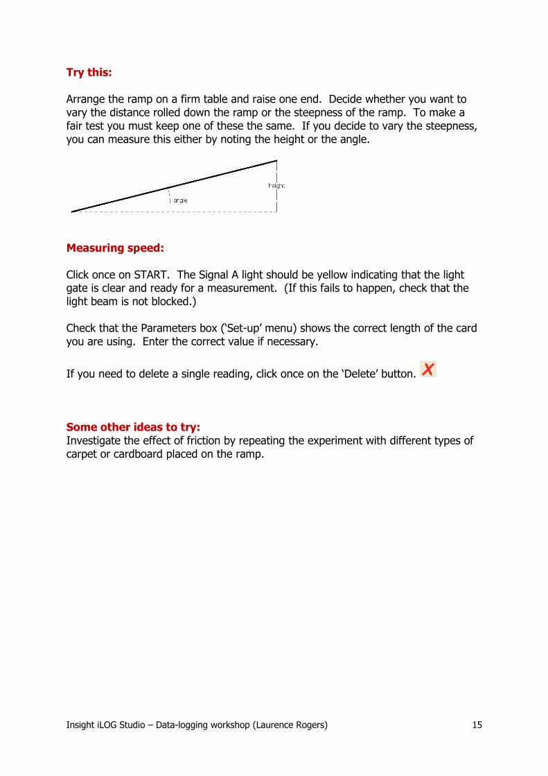
Cut out a piece of card like that shown (black card is best) and fix it on the top of the car. Set up the light gate on the slope so that as the car rolls down the card passes through and cuts the light beam.


Try this: Arrange the ramp on a firm table and raise one end. Decide whether you want to vary the distance rolled down the ramp or the steepness of the ramp. To make a fair test you must keep one of these the same. If you decide to vary the steepness, you can measure this either by noting the height or the angle.

Measuring speed: Click once on START. The Signal A light should be yellow indicating that the light gate is clear and ready for a measurement. (If this fails to happen, check that the light beam is not blocked.) Check that the Parameters box (‘Set-up’ menu) shows the correct length of the card you are using. Enter the correct value if necessary.

If you need to delete a single reading, click once on the ‘Delete’ button. Some other ideas to try: Investigate the effect of friction by repeating the experiment with different types of carpet or cardboard placed on the ramp.


Conduction of heat

The thermal conductivity of four different metals can be compared using a traditional piece of apparatus and a data-logging system.

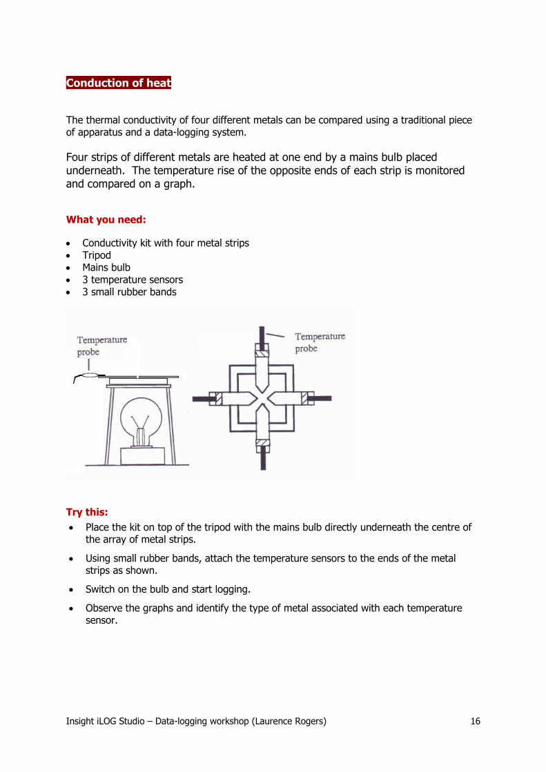
Four strips of different metals are heated at one end by a mains bulb placed underneath. The temperature rise of the opposite ends of each strip is monitored and compared on a graph.

What you need:

Conductivity kit with four metal strips Tripod Mains bulb 3 temperature sensors 3 small rubber bands

Try this:

Place the kit on top of the tripod with the mains bulb directly underneath the centre of the array of metal strips.

Using small rubber bands, attach the temperature sensors to the ends of the metal strips as shown.

Switch on the bulb and start logging.

Observe the graphs and identify the type of metal associated with each temperature sensor.



Click on to show the cursor. As you move the cursor across the graph, the bar display shows how the temperature varied during the experiment.

Which metal showed the fastest rise in temperature?

Take readings from your graph

What was the temperature at the start of the experiment?

What were the temperatures of each metal after 10 minutes?

List the metals in order of thermal conductivity.

Find out how big the change was (Use ‘Change’)

Find out the temperature change for each metal during the experiment.

Find out the rate of change of temperature for each metal (Use ‘Rate’)

How uniform was the rise in temperature for each metal?

Discussion and evaluation: Is conduction along the metals the only way the energy can reach the temperature probes? What questions should be asked about the fairness of the test? Is the position of the bulb important? What results might be expected if the bulb were placed off-centre? You could try this.


Walkabout: Measuring motion

In this experiment you will:

use the motion sensor to obtain distance-time graphs of your motion as you walk in front of the sensor

think about how the shape of the graph is related to your motion

obtain measurements from the graph to find out your speed

plot a speed-time graph of your motion

What you need:

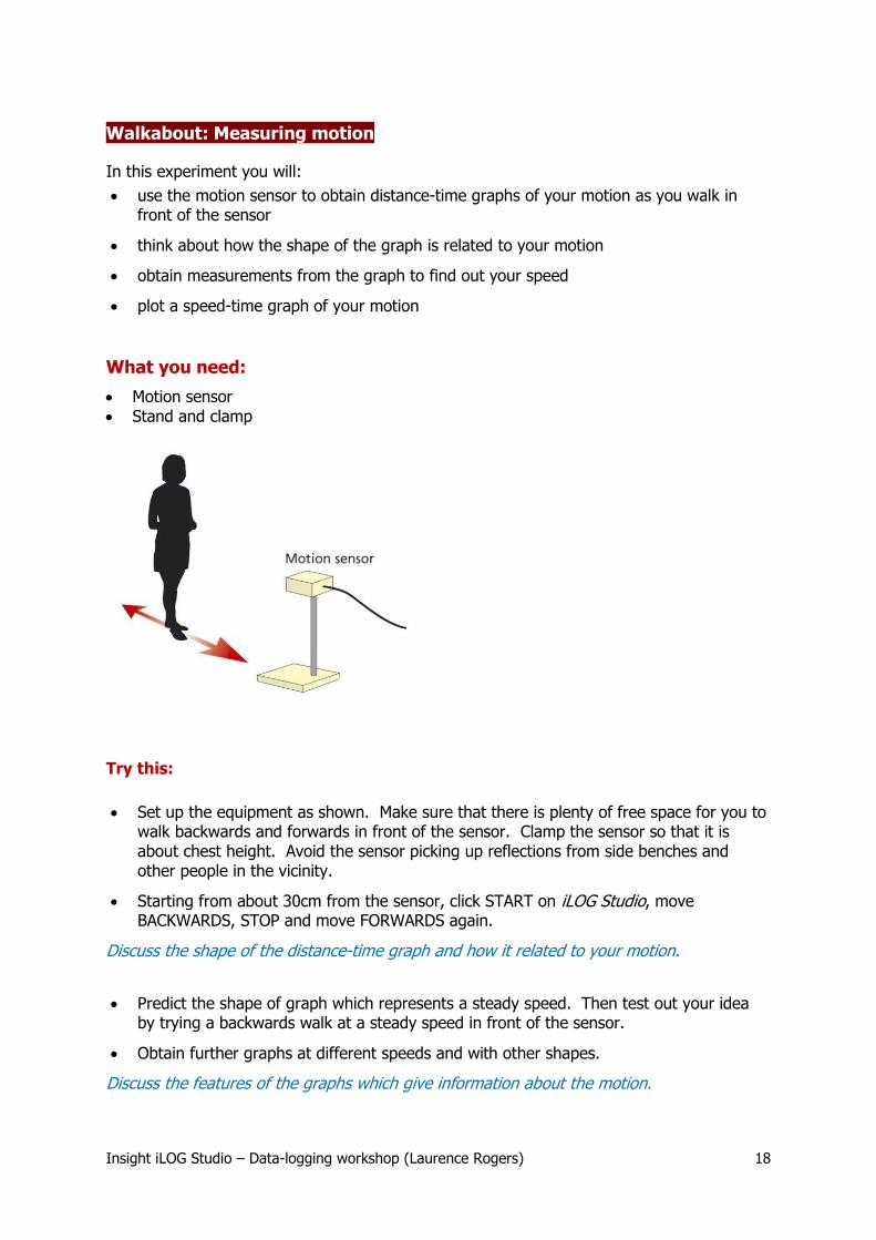
Motion sensor Stand and clamp

Try this:

Set up the equipment as shown. Make sure that there is plenty of free space for you to walk backwards and forwards in front of the sensor. Clamp the sensor so that it is about chest height. Avoid the sensor picking up reflections from side benches and other people in the vicinity.

Starting from about 30cm from the sensor, click START on iLOG Studio, move BACKWARDS, STOP and move FORWARDS again.

Discuss the shape of the distance-time graph and how it related to your motion.

Predict the shape of graph which represents a steady speed. Then test out your idea by trying a backwards walk at a steady speed in front of the sensor.

Obtain further graphs at different speeds and with other shapes.

Discuss the features of the graphs which give information about the motion.


Looking at your results: Taking measurements from the graph

Click on to show the cursor. As you move the cursor across the graph, the bar display shows how you moved during the experiment.

From the graph, find out the furthest distance recorded by the sensor.

Select ‘Change’ and ‘Interval’ and use these to find the distance moved in 1 second at different places on the graph.

How can you use these measurements for calculating speed?

Speed measurements can be calculated directly using ‘Gradient’:

Select ‘Gradient’ on the ‘Analyse’ menu and move the cursor across the graph to measure the gradient at different points. (RIGHT click near the graph line to make the gradient cursor show.)

Find the point on the graph where the velocity is a maximum.

Further work

Show channel V which gives a speed vs. time graph for the motion.

Record a graph for walking at a steady speed, then look carefully at the speed graph for evidence of your reciprocating leg movement whilst walking.


Antacids

It is usual for your stomach to contain dilute acid which helps the body to digest food. However, if there is too much acid present then you may suffer from acid indigestion. A common cure for acid indigestion is to take an antacid which stops acid indigestion by neutralising the acid in the stomach with a mild alkaline substance. In this experiment the acid in the stomach is simulated by cola drink. Using a pH probe you can measure its acidity and then find out how the acidity changes when you add an antacid tablet. It is interesting to compare the effect of crushing the tablet first before adding it to the cola. How do you think it might affect the results?

The experiment

What you need:

Two 100 ml beakers Cola drink Antacid tablets (e.g. Alka Seltzer) ph probe and connector Wash bottle with distilled water

Try this:

Half fill each beaker with cola drink.

Insert the pH probe into one beaker.

Start logging. Then, after 2 minutes drop a tablet into the cola and observe the change of pH as it dissolves.

Wash the pH probe with distilled water, and repeat the experiment with the second beaker of cola, but this time crush the tablet before dropping it into the drink.

Note that the ‘Overlay’ option is ticked on the ‘Set up’ menu so that the results from the second experiment appear on the same graph axes.



Show the data just for the first experiment.

Click on to show the cursor. As you move the cursor across the graph, the bar display shows how the pH value varied during the experiment.

How long did it take the pH probe to show a steady reading?

At what point on the graph was the tablet added?

By how much did the tablet reduce the pH?

Might the tablet be useful for curing stomach pains?

Compare the graphs from the two experiments

Show the data from the second experiment together with the first set. If you wish you can show the data with separate pairs of axes by pressing Ctrl + G.

Compare the two graphs, looking at the time for changes, the rates of change and the overall reduction of pH.

What effects did the crushing of the tablet have on the changes of pH?

Further work:

Investigate the effect of adding a second tablet when the first has dissolved.

Investigate the effect of dissolving the tablet in water first and adding the solution to the Cola.

Try different brands of antacid tablets and powders and compare them to see which are the most effective.


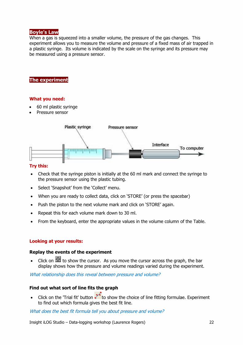
Boyle’s Law When a gas is squeezed into a smaller volume, the pressure of the gas changes. This experiment allows you to measure the volume and pressure of a fixed mass of air trapped in a plastic syringe. Its volume is indicated by the scale on the syringe and its pressure may be measured using a pressure sensor.

The experiment

What you need:

60 ml plastic syringe Pressure sensor

Try this:

Check that the syringe piston is initially at the 60 ml mark and connect the syringe to the pressure sensor using the plastic tubing.

Select ‘Snapshot’ from the ‘Collect’ menu.

When you are ready to collect data, click on ‘STORE’ (or press the spacebar)

Push the piston to the next volume mark and click on ‘STORE’ again.

Repeat this for each volume mark down to 30 ml.

From the keyboard, enter the appropriate values in the volume column of the Table.


Click on to show the cursor. As you move the cursor across the graph, the bar display shows how the pressure and volume readings varied during the experiment.

What relationship does this reveal between pressure and volume?

Find out what sort of line fits the graph

Click on the 'Trial fit' button to show the choice of line fitting formulae. Experiment to find out which formula gives the best fit line.

What does the best fit formula tell you about pressure and volume?


Calculate ‘pressure x volume’

Click on the ‘Formula’ button select ‘New’.

Name the new data ‘P x V’

In the Formula dialogue box, create the formula ‘A = P x V’.

Plot a bar chart of the new column of data. (Click on the column heading, then click

Notice how the values for P x V are very similar. What does this tell you about the pressure and volume?

How is this relationship stated in Boyle’s Law?

Further work As an alternative method of analysing the pattern in the results, calculate values for ‘1 / volume’ and then show their relationship with pressure on a new graph:

Click on the ‘Formula’ button select ‘New’.

Name the new data ‘1 / V’

In the Formula dialogue box, create the formula ‘B = 1 / V’.

Change the horizontal axis to show ‘1 / V’


Change of state

For every substance there is a special temperature at which it changes from solid to liquid. This is called the 'Melting point' and it is a different temperature for each substance. The natural state of the substance depends upon whether its melting point is above or below room temperature: SOLID: the melting point is ABOVE room temperature LIQUID: the melting point is BELOW room temperature The melting point of ice cream is below room temperature, which is why it usually melts when it is taken out of the fridge. In this experiment you will investigate the melting point of a substance which is above room temperature: Stearic acid is normally a white crystalline solid. However, when it is heated up in a bath of boiling water it melts into a liquid. When you let it cool gradually, it becomes solid again. With the aid of the computer you can record the temperature as it cools and display the results in the form of a 'cooling curve' on a graph. To investigate the change between liquid and solid, here are some of the questions you might ask during the experiment: How can you tell from the graph which part shows the liquid state?

Which part showed the solid state?

At what temperature did the liquid start solidifying?

How long did it take for the liquid to solidify?

What does the shape of the graph tell you about the loss of heat by the substance?

The experiment

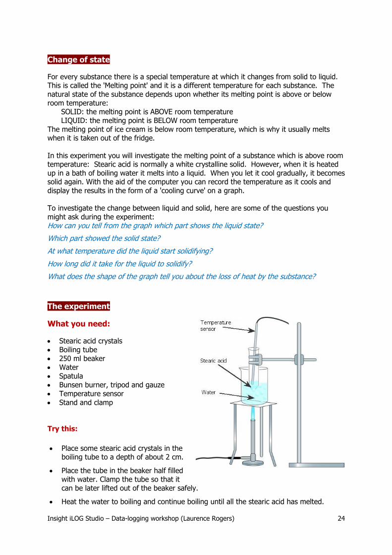
What you need:

Stearic acid crystals Boiling tube 250 ml beaker Water Spatula Bunsen burner, tripod and gauze Temperature sensor

Stand and clamp Try this:

Place some stearic acid crystals in the boiling tube to a depth of about 2 cm.

Place the tube in the beaker half filled with water. Clamp the tube so that it can be later lifted out of the beaker safely.

Heat the water to boiling and continue boiling until all the stearic acid has melted.


Carefully insert the temperature probe into the boiling tube. Boil the water for another half minute.

Start logging (20 minutes), stop heating the water and carefully lift out from the beaker the boiling tube, keeping it in the clamp.

Stir the substance gently as long as possible, using the probe. Look out for interesting changes on the graph as the experiment progresses.



Look for the part of the graph where the temperature hardly changed.

Recall what you saw happening to the stearic acid at this stage of the experiment.

Add captions to your graph

Decide which part of the graph records the liquid state of the substance. Add a caption to the graph to label this part of the graph liquid.

Decide which part of the graph recorded where the substance had changed into the solid state and label that part with a caption solid.

Add another caption to show the change from liquid to solid.

Take readings from your graph What was the highest temperature during the experiment?

What was the lowest temperature?

The temperature indicated by flat part of the graph is called the 'melting point'. What value does your graph show for this? Measure the changes of temperature (Use ‘Change’) Over what range of temperature was the substance in the liquid state?

Measure the time for change (Use ‘Interval’) How long did it take for the substance to make the change from liquid to solid?

Measure the rate of change (Use ‘Gradient) At which part of the experiment did the temperature change at its maximum rate?

Further work

Repeat the experiment with the tube placed in a larger tube containing cold water: Use a second temperature probe to record how quickly the cold water warms up and compare this change with the changes in the temperature of the cooling substance.


Evaporation and cooling

Do you feel cold when you get out of a swimming pool? Does your skin feel cold when you spill after shave or perfume on it? Both these effects are due to evaporation of a liquid from your skin. When a liquid evaporates it causes a cooling in the surface it leaves behind. Evaporation takes place at the surface of a liquid and it consists of the liquid changing into a vapour or gas. Energy is needed to convert a liquid into a vapour, so when the vapour escapes, it carries away thermal energy and leaves the liquid cooler. The purpose of this experiment is to investigate the cooling effect, to find out how different factors affect the amount and rate of cooling. Here are some of the questions you can ask about the process:

How quickly does the liquid cool?

How long does the cooling last?

Do different liquids cool at different rates?

Does the cooling depend on the amount of liquid?

Does the cooling depend upon the temperature of the air?

The experiment

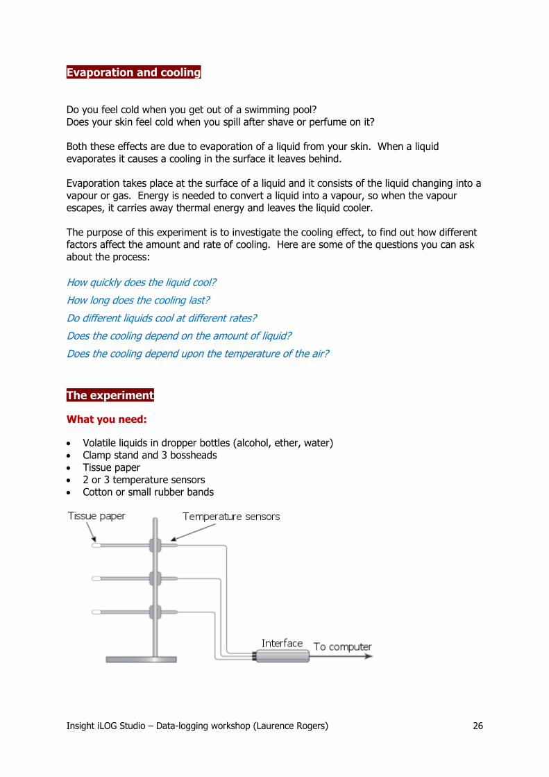
What you need:

Volatile liquids in dropper bottles (alcohol, ether, water) Clamp stand and 3 bossheads Tissue paper 2 or 3 temperature sensors Cotton or small rubber bands


Try this:

Clamp the temperature sensors in a stand as shown.

Wrap a small piece of tissue paper around the tip of each sensor. Secure the paper with some cotton or a staple.

Start logging and use a pipette to add two drops of alcohol on to the tissue paper on one sensor.

Notice how the liquid cools the temperature probe.

Looking at your results: Take readings from your graph

What was the temperature at the start of the experiment?

How low did the temperature go?

Replay the events of the experiment


How did the alcohol affect the temperature of the probe?

Find out how big the change was (Use ‘Change’)

How much did the temperature change during the experiment?

Find out how long the change took to occur (Use ‘Interval’)

How long did it take for the temperature to drop to its lowest point?

Comparing three liquids Now do an experiment to find out which of the three liquids has the greatest cooling effect. To make your experiment a fair test, use the same number of drops of each liquid.


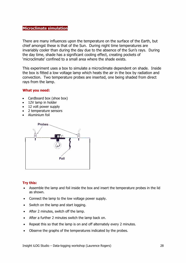
Microclimate simulation

There are many influences upon the temperature on the surface of the Earth, but chief amongst these is that of the Sun. During night time temperatures are invariably cooler than during the day due to the absence of the Sun’s rays. During the day time, shade has a significant cooling effect, creating pockets of ‘microclimate’ confined to a small area where the shade exists. This experiment uses a box to simulate a microclimate dependent on shade. Inside the box is fitted a low voltage lamp which heats the air in the box by radiation and convection. Two temperature probes are inserted, one being shaded from direct rays from the lamp. What you need:

Cardboard box (shoe box) 12V lamp in holder 12 volt power supply 2 temperature sensors Aluminium foil

Try this:

Assemble the lamp and foil inside the box and insert the temperature probes in the lid as shown.

Connect the lamp to the low voltage power supply.

Switch on the lamp and start logging.

After 2 minutes, switch off the lamp.

After a further 2 minutes switch the lamp back on.

Repeat this so that the lamp is on and off alternately every 2 minutes.

Observe the graphs of the temperatures indicated by the probes.



Click on to show the cursor. As you move the cursor across the graph, the bar display shows how the temperatures varied during the experiment.

Which temperature probe showed the greatest variation?

Explain why the temperatures in different parts of the box vary differently.

Take readings from your graph

What were the temperatures indicated at the start of the experiment?

What was the highest temperature indicated by each probe?

Find out about the changes of temperature (Use ‘Change’)

Measure the largest temperature variation for each probe.

Find out about the difference between the two sets of readings (Use ‘Difference’)

Measure the largest temperature difference between the two probes.

Find out the average temperatures (Use ‘Average’)

Measure the average temperature indicated by each probe.

Discussion and evaluation: What factors contributed to the different average temperatures recorded for the two probes? What are the implications of sunlight and shadow on astronauts in space? How do conditions in the experiment differ from those in space? Consider the extremes of temperature that are likely to be recorded. Consider the similarities and differences between the experiment and the climate on Earth during night and day.


Rate of reaction

Some chemical reactions are faster than others and one of the factors which affect this is the concentration of the chemical solutions being mixed. Take the reaction between sodium thiosulphate and hydrochloric acid: When you mix the two clear solutions they form a precipitate of sulphur which makes the solution go cloudy. If you use more concentrated solutions, this happens more quickly. You can measure how quickly this happens by using a light sensor connected to a computer. The precipitate is detected by measuring the amount of light passing through the mixture. You can find out how the rate of reaction is related to the concentration of the two solutions. Here are some of the questions you can ask about the process:

How long does it take for the reaction to start after the solutions are mixed?

Does the reaction proceed at a steady rate?

How do you know when the reaction has finished?

How long does it take the reaction to finish?

If you dilute the solution, how does this affect the reaction time?

The experiment

What you need:

100 cm3 beakers

50 cm3 measuring cylinder 5 cm3 syringe 50 cm3 1M hydrochloric acid 250 cm3 1M sodium thiosulphate solution Distilled water Clamp stand, clamps and electric lamp or torch Light sensor

Try this:

Assemble the equipment as shown.

Place 50 cm3 of sodium thiosulphate in the beaker and draw 5 cm3 into the syringe.

Start logging and use the syringe to add 5 cm3 of acid into the flask. (The squirt action of the syringe usually gives a good stir). Watch the trace on the computer screen as the reactants form a precipitate.

Stop logging when there is no further change.

To show how concentration affects the reaction you will need to repeat the experiment with different dilutions of sodium thiosulphate as follows:

1. Add 10 cm3 distilled water to 40 cm3 sodium thiosulphate. 2. Add 20 cm3 distilled water to 30 cm3 sodium thiosulphate. 3. Add 30 cm3 distilled water to 20 cm3 sodium thiosulphate. 4. Add 40 cm3 distilled water to 10 cm3 sodium thiosulphate.


Between each of your experiments you should save your results on the disk so that you have a series of graphs. You may also put the graphs on the same axis as you do the experiments. You do this by first selecting ‘Overlay’ from the ‘Set up’ menu. Each time you click on START to do a new experiment, a graph will be added to the ones already on the screen.


Click on to show the cursor. As you move the cursor across the graph, the bar display shows how the readings varied during the experiment. Do this showing just one channel at a time and then compare them altogether.

Notice how the rate of change varies during the reaction.

Note also the little dip in the reading which shows when the acid was added.

Which graph line shows the most rapid reaction? Find out how long it took for a change to show


Select 'Interval' from the 'Analyse' menu.

Move to the point on the graph which shows when the acid was added (Look for the dip). Double click the mouse. Then move the cursor to the point where the change just begins to show and note the 'Interval' time.

Repeat this for each graph.

Which graph line shows the most rapid start for the reaction? Find out the maximum rate of change


Select 'Gradient' from the 'Analyse' menu. This measures the steepness of the graph at any point.

Find out the steepest point on the graph where the gradient is a maximum.

Repeat this for each of your graphs.

Which graph line shows the greatest maximum gradient? Find out the average rate of change


Select ‘Rate’ and 'Interval' from the 'Analyse' menu.

Adjust the time interval so that it spans the straight section on the steepest part of the graph line and make a note of the rate of change.

Repeat this for each of your graphs.

How does the rate of change depend upon the dilution of the sodium thiosulphate?


Why do small animals huddle? ((From Insight iLOG Junior – KS3)

Small mammals, such as mice and voles, often remain close together in their nest. Other animals, such as woodlice, also huddle. Do all small animals huddle for the same reasons? You can investigate huddling using a cluster of small tubes containing warm water and kept in close contact with each other by an elastic band. Think of each tube as an ‘animal’.

The experiment

What you need:

7 tubes or plastic drinking cups.

Warm water (from a hot tap; as hot as you can get, without scalding yourself).

A beaker or jug in which to stand your tubes.

2 or 3 temperature sensors. (If only two sensors are available, place one in the

middle tube and the other in the separate tube.)


Try this:

Pour the same volume of warm water into each of the tubes. Place the sensors as shown and start logging. Notice how the different tubes cool at differing rates. Looking at your results: Do your results show that huddling works?

Where is the best place in the huddle?

Some other ideas to try: There are lots of experiments you can try to find out what affects the cooling down of objects: Hot water in containers of different shapes and sizes.

Containers made of different materials.

Containers wrapped in wool, cloth, plastic, bubble-wrap etc.

ICT WORKSHOP FOR SCIENCE PGCE February … Studio Set-up texts (Feb...ICT WORKSHOP FOR SCIENCE PGCE...

Documents

Transcript of ICT WORKSHOP FOR SCIENCE PGCE February … Studio Set-up texts (Feb...ICT WORKSHOP FOR SCIENCE PGCE...