
ICT Call 8elib.dlr.de/98046/1/COLOMBO_D1.1_ScenariosExtensions_v2.4.pdfSmall or medium-scale focused...
57
Small or medium-scale focused research project (STREP) ICT Call 8 FP7-ICT-2011-8 Cooperative Self-Organizing System for low Carbon Mobility at low Penetration Rates Document Information Title Deliverable 1.1 - Scenario Specifications and Required Modifications to Simulation Tools Dissemination Level PU (Public) Version 2.4 Date 15.02.2014 Status Final Version with Review Comments COLOMBO: Deliverable 1.1 Scenario Specifications and Required Modifications to Simulation Tools
Transcript of ICT Call 8elib.dlr.de/98046/1/COLOMBO_D1.1_ScenariosExtensions_v2.4.pdfSmall or medium-scale focused...

Small or medium-scale focused research project (STREP)
ICT Call 8 FP7-ICT-2011-8
Cooperative Self-Organizing System for low Carbon Mobility at low Penetration Rates
Document Information Title Deliverable 1.1 - Scenario Specifications and Required
Modifications to Simulation Tools Dissemination Level PU (Public) Version 2.4 Date 15.02.2014 Status Final Version with Review Comments
COLOMBO: Deliverable 1.1 Scenario Specifications and Required
Modifications to Simulation Tools

COLOMBO: Deliverable 1.1; 2014-02-17
2
Authors Daniel Krajzewicz (DLR), Robbin Blokpoel (PEEK), Wolfgang Niebel (DLR), Jérôme Härri (EURE), Luca Foschini (UNIBO), Paolo Bellavista (UNIBO), Thrasyvoulos Spyropoulos (EURE), Laura Bieker (DLR)

COLOMBO: Deliverable 1.1; 2014-02-17
3
Table of contents
1 Introduction ................................................................................................................................... 5
1.1 Project Context ...................................................................................................................... 5
1.2 Document Objectives ............................................................................................................ 6
1.3 Task/Work Motivation .......................................................................................................... 6
1.4 Task/Work Structure ............................................................................................................. 6
2 State of the Art .............................................................................................................................. 7
2.1 Models and Simulation .......................................................................................................... 7
2.2 Scenario Classification .......................................................................................................... 8
2.3 Publicly Available Scenarios............................................................................................... 10
2.4 Assessment and Evaluation ................................................................................................. 10
2.5 Simulation Guidelines ......................................................................................................... 12
2.6 Scientific Literature ............................................................................................................. 12
3 COLOMBO Performance Indicators .......................................................................................... 15
3.1 Road Network PIs ............................................................................................................... 16
3.2 Intersection PIs .................................................................................................................... 17
3.3 Measurements ...................................................................................................................... 18
3.4 Communication PIs ............................................................................................................. 20
4 COLOMBO Scenarios ................................................................................................................ 25
4.1 Constraints and initial Considerations ................................................................................. 25
4.2 Real-World Scenarios.......................................................................................................... 28
4.2.1 Available Scenarios...................................................................................................... 28
4.2.2 Scenario Comparison ................................................................................................... 36
4.3 Synthetic Scenarios ............................................................................................................. 37
4.3.1 Generating synthetic Networks .................................................................................... 39
4.3.2 Generating synthetic Demands .................................................................................... 44
4.3.3 Further Notes................................................................................................................ 46
4.3.4 Deployment .................................................................................................................. 46
5 Needed Extensions ...................................................................................................................... 48
5.1 SUMO ................................................................................................................................. 48
5.2 ns-3 ...................................................................................................................................... 50
5.3 iCS ....................................................................................................................................... 51
5.4 Application Module ............................................................................................................. 53
6 Summary ..................................................................................................................................... 55
Appendix A – References .................................................................................................................. 56

COLOMBO: Deliverable 1.1; 2014-02-17
4

COLOMBO: Deliverable 1.1; 2014-02-17
5
1 Introduction
1.1 Project Context The COLOMBO project will deliver a set of modern cooperative traffic surveillance and control applications that target at different transport related objectives such as increasing mobility, resource efficiency, and environmental friendliness.
The surveillance applications use information gained via vehicular communication technology at low penetration rates (WP1). The traffic control applications are of self-organizing type using swarm intelligence methods (WP2). They are optimised based on simulations-in-the-loop (WP3). To allow the ex-ante appraisal of the applications’ impacts, the evaluation framework must be defined. It has design interdependencies with the traffic simulation scenarios which trigger modification and extension requirements to existing simulation tools. Once realized they are implemented into a dedicated software suite which is mainly open source (WP5). Since the work takes into consideration the vehicular population in the year 2020, respective adaptations like the inclusion of electrical vehicles is essential (WP4).
Figure 1.1: COLOMBO work packages
While the simulation system itself – the computer applications used to perform the simulations – was already defined in the project’s Description of Work [COLOMBO, 2012] and described in detail in the project’s deliverable D5.1 “Prototype of overall System Architecture and Definition of Interfaces” [COLOMBO D5.1, 2013], the used scenarios as well as the used performance indicators and measures are of similar importance.

COLOMBO: Deliverable 1.1; 2014-02-17
6
1.2 Document Objectives The objectives of this document are to point out the need for a common methodology to appraise and benchmark traffic surveillance and traffic light algorithms, to present the underlying performance indicators (PIs) with their measurements, to show the defined traffic simulation scenarios as part of the experimental design, and to describe how the simulation system must be extended to meet the requirements set by these definitions.
1.3 Task/Work Motivation Modern technology is usually tested and evaluated ex-ante, i.e. before being deployed in the real world, saving deployment costs during (repeated) tests and reducing risks opposed to real world by malfunctioning or not properly designed systems.
As a good and common practice, the presented technology is tested in a single or multiple scenario(s) – a combination set of spatial, temporal, regulatory, behavioural, and technological control parameters. The outcomes are then either benchmarked with the beforehand defined goals or compared to an existing baseline, showing the gains and losses of the new attempt. But bad prepared scenarios can yield in a non-realistic representation of traffic. Also, scenarios can be tailor-made to show benefits for a certain type of application while suppressing unwanted effects. The same counts for the selected measurements, which may not report on disadvantages.
There seems to be a large number of different kinds of scenarios and measurements in literature to benchmark the described algorithms of traffic surveillance or traffic control. Moreover, they are usually incompletely described and thus not reproducible.
Thereof, the motivation of this task is twofold. On a short term, the COLOMBO project shall be equipped with a set of scenarios that allow to measure the performance of the developed solutions. The developed scenarios will be used in subsequent tasks performed in WP1 (traffic surveillance algorithms), WP2 (traffic light controls), and WP4 (emission-optimal driver behaviour and traffic lights). In a long term, the set of scenarios shall be integrated into a well-defined traffic light algorithms evaluation framework that shall introduce a methodology to determine how good an investigated solution works under which circumstances. In addition, it will make evaluations of traffic light algorithms – and other traffic applications as well – comparable, raising the scientific quality of such experiments. This methodology will be developed and coded within the software suite in COLOMBO’s WP 5.3.
Until now the COLOMBO overall simulation system (COSS) supports only the traffic modes of motorized private, public, and freight vehicles. Since multimodal evaluations make more and more their way into the focus, the scenarios must account for this by including pedestrians and bicyclists. This poses additional requirements to the COSS that will be discussed within this report, too.
1.4 Task/Work Structure The document is organised as following. In Chapter 2, the state of the art in evaluating traffic management applications is given, with a focus on traffic lights. Then, the performance indicators that shall be used in later steps of the COLOMBO project are given in Chapter 3. Chapter 4 presents the scenarios generated within the project, including an overview about the real world scenarios that were made available within the project as well as the description of a tool developed within the project that realises the generation of synthetic scenarios. Needed extensions to the involved simulation applications are described in Chapter 5. The document ends with a summary, given in Chapter 6.

COLOMBO: Deliverable 1.1; 2014-02-17
7
2 State of the Art
2.1 Models and Simulation For a large number of approaches to observe and to control traffic described in literature, such investigations are performed using traffic simulation software tools. A simulation always needs a parameterised model for how its objects are (inter-)acting as an abstracted representation of the real world behaviour. On a top level, traffic simulations are conventionally classified by the granularity of the traffic representation. Coarse macroscopic traffic (flow) simulations describe how an aggregated stream of vehicles propagates through a given network. Fine microscopic simulations model each vehicle explicitly and compute the traffic flow’s progression by modelling each vehicle’s speed and lane choice, mostly using discrete time steps of one second or less. Briefly spoken, each participant follows her/his wishes to move forward, avoiding collisions with other traffic participants and following the regulations under different constraints. Further differentiations can be found in literature such as [Laval, n.d.] or [Akcelik, 2007], shown in Figure 2.1 and Figure 2.2.
Figure 2.1: Types of Simulation in Transportation [Laval, n.d.]

COLOMBO: Deliverable 1.1; 2014-02-17
8
Figure 2.2: Road Traffic Models [Akcelik, 2007]
COLOMBO investigations need the microscopic view for different reasons. First, it enables the necessary model extension by simulating the communication in a Mobile Ad Hoc Network (MANet), specifically a Car-to-X (C2X) network. This requires information about the vehicles' positions. The necessity for this model extension lies in the dependency of the vehicles’ behaviour from the communication characteristics and is outlined, e.g., in [Sommer et al., 2008].
Second, the assignment of different equipment rates to vehicles is easier within microscopic simulations. Last, only microscopic simulations represent the acceleration and deceleration of single vehicles, what has a strong impact on the accuracy of emission computation.
To ensure the built model represents the reality accurately enough, it needs to be calibrated and validated with data from reality, i.e. without any implemented application to be evaluated. Respective guidelines are described in sect. 2.5. Once a valid simulation model is ensured, the evaluated traffic management application can be embedded, either by implementing it directly into the used traffic simulation or by influencing the traffic simulation via an API by an external module which replicates the application.
Having each vehicle’s movement at each time step at hand, microscopic traffic simulations are capable to compute a large number of data, among them single vehicles’ speed, acceleration, or position. Usually, these measured data are further processed, e.g., aggregated and transformed into performance indicators (PI). The measurements and PIs used by COLOMBO are presented in detail in chapter 3.
These values are calculated for a given scenario, which is a combination set of spatial, temporal, regulatory, behavioural, and technological control parameters that cannot be changed by the simulation itself. These exogenous parameters can either be static or dynamic, defining the road network layout, a traffic demand, participants’ reactions, technological equipment and physical restrictions.
2.2 Scenario Classification
Constituting Scenario Object Parameters
As the simulated objects need to be parameterised within the different aforementioned parameter classes, a scenario classification can be executed by distinguishing their respective value ranges. Objects do not necessarily contain parameters of all classes.

COLOMBO: Deliverable 1.1; 2014-02-17
9
The most common parameters of the road network and infrastructure objects are of spatial and regulatory kind. Often, the road network is represented as a 2D graph, which nodes represent the road network’s intersections, while edges represent its roads. It might become necessary to include the altitude of nodes and the resulting inclination of edges to form a 3D model. The regulatory parameters comprise speed limits on edges as well as the applied right-of-way-signalisation at junctions including traffic lights. As signal times and plans incur predefined (periodic) changes they have temporal parameters, too. Other infrastructure elements should be considered, depending on the performed research. Traffic demand of the traffic participants has above all spatio-temporal parameters like their origins and destinations which are also time-dependant (the 4th dimension). The demand is often not modelled by listing all vehicles explicitly, but rather by defining “flows” or “streams” consisting of a number of vehicles that share certain technological parameters or their distribution. Nonetheless, special kinds of participants, such as public transport or emergency vehicles are often modelled explicitly. The origin-destination-matrices (O/D) describe how many vehicles move from one area (origin) to another one (destination) during a certain time period. Such demand descriptions are usually used when simulating larger areas, but may be also applied to smaller road networks.
Additionally to the technological parameters of vehicles their drivers are described with behavioural parameters, which often pose a big challenge to the modeller since they represent difficult to observe psychological decisions.
All parameters of the modelled objects must be set in the suitable granularity depending on the needs of the experiment. Amongst them but not all-encompassing are the following:
• Spatial (Network layout) • Number, position and interconnection of nodes, spanning from single intersection to linear
corridors and meshed networks • Number, position and length of lanes • traffic light positions • pedestrian crossings • bus stops • sensors (for calibration and validation)
• Temporal • Start and end time, time of state changes • traffic demand load curves • signal time plans
• Regulatory • speed limits on edges • right-of-way-signalisation • limitations of infrastructure usage to particular vehicle categories
• Technology • vehicle types and categories incl. combustion technology • V2X equipment penetration rate
• Behaviour • Driving style (sub-models for car following, lane change etc.) • Participants’ adherence to regulatory settings and advices
Events or the weather are not direct model parameters but must be converted into the aforementioned ones. Rain for example might lead to slippery roads and reduced sight, leading to decreases in the vehicles’ velocities and a more careful and defensive driver behaviour. Such behavioural changes would be reflected in simulation parameters, such as the driver’s preferred velocities and time headways.

COLOMBO: Deliverable 1.1; 2014-02-17
10
As each vehicle’s movement is individually computed, microscopic traffic simulations are usually very sensible to errors in the spatial and behavioural description. Special care should be taken when defining the number of lanes (including an increment in lane numbers in front of intersections), the speed limits, and the right-of-way and direction-of-drive rules at intersections.
Real World vs. Synthetic Scenarios
Within descriptions of evaluating traffic management applications, one can find two types of used scenarios: a) attempts to replicate a part of a real world network and b) purely synthetic scenarios where the “Manhattan grid” is one well-known example. Almost every time the scenarios are non-disclosed and tailor-made exclusively for the investigation, thus serving only the specific single-usage.
For some investigations, a synthetic road network may have a larger benefit, as it allows to model and concentrate on a certain, well-defined and less complex setting and so to investigate certain behaviour more explicitly. In addition, one has a higher degree of control on a synthetic scenario’s attributes, what again helps in determining the evaluated system’s dynamics. Real-world networks often “blur” the results, by mixing different types of transport and they are usually too complex to easily understand the underlying dynamics.
Evaluations of traffic management applications using complex real-world scenarios allow determining whether the application can handle the real life’s complexity at all. Often, well prepared real-world scenarios include structures that can be rarely found in synthetic scenarios, such as a high variety of public transport modes including their delays, pedestrians, complex intersection geometries, etc.
Finally, one should state that usually every traffic light is planned within a computer simulation explicitly before being deployed in the real world. Here, the real world intersection that shall be later controlled by the designed traffic light is modelled, of course.
2.3 Publicly Available Scenarios Beside the single-usage scenarios which require a lot of setup work for a limited output and hence yield a doubtful effectivity, some yet academic simulation users offer their built scenarios and data sets for disclosed multi-usage by the entire community. As an example this movement the NGSIM (Next Generation SIMulation Community) members can be found, who put the following data sets on the free accessible webpage [NGSIM, 2013]:
• 45 min afternoon peak at Interstate 80 in Emeryville (San Francisco), California • 45 min at U.S. Highway 101 (Hollywood Freeway) in the Universal City neighbourhood of Los
Angeles, California • 30 min morning peak at Lankershim Boulevard in the Universal City neighbourhood of Los
Angeles, California • 30 min at Peachtree Street in the Midtown neighbourhood of Atlanta, Georgia • Sample dataset from ATLAS/University of Arizona • Sample data from University of California at Berkeley Highway Laboratory.
2.4 Assessment and Evaluation A modern and comprehensive project evaluation needs to be planned from the beginning on, as it has heavy design impacts on all levels of the application development and simulation experiment. Briefly described global project objectives need to be broken down into sub-goals, also called criteria. These criteria can be interpreted as the research question if and to which extent the investigated application helps to achieve the initial objectives. Transport-related global objectives can be named as the following six: Mobility, Resource Efficiency, Environmental Impact, Safety,

COLOMBO: Deliverable 1.1; 2014-02-17
11
Security, and User Experience, based on [Transport Canada, 2007] and others. Some of these objectives can also be transferred to evaluate communication networks. Obviously, derived criteria for both fields are different.
Criteria are made operational by defining performance indicators (PIs). According to [FESTA, 2008], a PI is a “[…] quantitative or qualitative measurement, agreed on beforehand, expressed as a percentage, index, rate or other [unit], which is monitored at regular or irregular intervals and can be compared with one or more criteria.”, emphasizing that “A denominator is necessary for a PI. A denominator makes a measure comparable (per time interval/per distance/in a certain location/…).” Measurements finally are the crisp values delivered by sensors in the case of field tests or the direct output of the simulation experiment. Synonymously used are the terms “Measure of Effectiveness” (MOE) [FHWA, 2004] and “Measure of Performance”. The impact assessment and evaluation on the acquired data can be executed with different methods and procedures on different levels of PI transformation, aggregation and synthesis, comprising mono- or multi-criteria approaches with the Cost-Benefit-Analysis being a widespread but challenging occurrence. Within this deliverable, only the PIs and their underlying measurements used within COLOMBO are presented. The evaluation procedures which make use of the PIs will be later described in deliverable D5.3, “Traffic Light Algorithm Evaluation System”. The difference shall be illustrated with a simple example. The average waiting time in seconds per vehicle is a PI, whereas the transformation into a “Level of Service” within the range of [A..F] already inherits an evaluative act. The way how PIs, measures, and the assessment are placed within the design process of experiments is shown in Figure 2.3 [FESTA, 2008]. The same source also contains a comprehensive overview about possible PIs and their measures.
Figure 2.3: FESTA’s V-Model of performing an FOT ([FESTA, 2008])
When evaluating a new traffic management application, usually it is done the relational way by comparing the base case before any alteration against the one after deploying the evaluated application. In a first step, the traffic of a particular period of interest, e.g. an average day, the peak time, or a special event, in a chosen scenario is set up and used for generating chosen measures. Then, the evaluated traffic management application is switched on. The simulation is performed once again, now with the traffic management application under evaluation. The results of both simulation runs are compared.
COLOMBO: Deliverable 1.1; 2014-02-17
12
On the opposite absolute procedures convert specific measures into a Level of Service (LoS) according to established guidelines, e.g., the US-American Highway Capacity Manual HCM [TRB, 2010] or the German Handbuch für die Bemessung von Straßenverkehrsanlagen HBS [FGSV, 2001]. This LoS can serve to evaluate the goodness of each single scenario even without any comparison to a base line.
2.5 Simulation Guidelines To carry out valid simulation studies some work steps have to be followed, including model building, calibration, validation, and statistical testing. They are described in several guidelines like “Traffic Analysis Toolbox Vol. III” (FHWA, 2004), “Simulation model calibration and validation” [VTRC, 2006],”Traffic Modelling Guidelines version 3.0” [TfL, 2010], “The use and application of microsimulation traffic models” [Austroads, 2006], “Hinweise zur mikroskopischen Verkehrsflusssimulation, Grundlagen und praktische Anwendung” [FGSV, 2006], as well as the simulation software manufacturers’ manuals.
Other issues which also might include rather voluntary best practice conformity than obligatory requests can be named according to [Brackstone et al., 2014]:
• Fall back strategies, absence of data, transferability • Relative effect of parameters on output, hierarchy of parameters • indicators to use • Differences in procedure according to scale and purpose • Sensitivity analysis and how to perform it • Definitions • How to structure a project/calibration activity • Warm up • Number of runs • Model specific issues.
2.6 Scientific Literature Currently, a rising awareness for good scientific practices can be observed. An increasing number of publications points out the issue of incompletely described simulation (read: experiment) settings that disallow any comparison of the results to any prior work. A recently conducted web based survey study [Brackstone, 2012] concentrated on questions concerning the size of the model, used simulation software, calibration, and validation.
Survey Design and Outcomes
To complement these “push”-triggered results from mainly commercial users, 40 rather academic publications that evaluate new traffic light algorithms were “pulled” and scanned. The following information was extracted from each of them:
• What kind of scenario (single intersection, corridor, network) was used and if it is properly described, including both the spatial and temporal parameters.
• Which measures and PIs were used and if they are properly defined. • Which traffic simulation software and which therein evaluated algorithm’s paradigm (fuzzy
logic, genetic algorithms, etc.) were used.
Both classifications of the last bullet point are reproduced as they may give hints about the context the publications have been performed within. Looking at the used traffic simulations (see Figure 2.4a), one can find a considerable number of self-developed software programs (10 of 42). Commercially available simulation packages, such as Vissim, CORSIM, Paramics, TRANSYT

COLOMBO: Deliverable 1.1; 2014-02-17
13
(each with multiple occurrence), AIMSUN, MATLAB, and Integration (each with one representation) are used in less than half of the papers. The emphasis on certain techniques from computer science, such as Neural Networks (NN), Q-learning, or genetic algorithms (see Figure 2.4b) is also higher than one would expect. It did not always become clear, whether the quality demands for scientific simulation studies as outlined in section 2.5 were fulfilled.
Figure 2.4: Papers on traffic light evaluation; (a) used traffic simulation; (b) major paradigm for the control
algorithm
Regarding performance indicators within the forty publications, 44 different PIs have been used to monitor the investigated traffic light algorithm. They can be grouped as shown in Figure 2.5 with “waiting time”, “queue size”, “delay”, and “travel time” used most often. Nonetheless, each of these four groups contains figures that differ between raw measurements and computed values, e.g., averages or rates, which are hardly comparable. Beside the fact that computing “delay” requires an interpretable definition of the desired target speed, this group as example is constituted by the following original paper names: “delay”, “average delay per vehicle per second”, “average delay per vehicle”, “delay at intersection”, “total mean delay”, “mean rate of delay“, “total delay”. It should also be mentioned, that only one of the examined publications gave a formula for the used measures – the others just named or described the used ones.
Figure 2.5: Papers on traffic light evaluation; PIs/measures by occurrence
The spatial 2D-scale of the examined scenarios ranges from a single intersection, over a corridor as several intersections in a line, to a road network with at least one. In 8 cases, a single intersection investigation serves as an initial proof before broadening into a corridor or a network. At all, 11 corridor, 20 network, and 19 single intersections scenarios were used. When looking how well the
10
5
4 4
4
4
2
9
own (unique)
undefined
SUMO
Vissim
CORSIM
TRANSYT
Paramics
other (known)
14
7 4 2 2
2
10
own (unique)
genetic / evolutionary
fuzzy logic
Q-learning
NN
game theory
other
02468
101214
none
wai
ting
time
thro
ught
put
queu
e siz
e
dela
y
trav
el ti
me
spee
d
envi
ronm
enta
l
othe
r

COLOMBO: Deliverable 1.1; 2014-02-17
14
scenarios are described, one has to realize that 89% of single intersections could be replicated using the information given in the according paper, but only 36% of corridors, and 20% of the networks. A 3D-model for the inclusion of the altitude could not be observed. The temporal 4th dimension spans between a single peak hour and 16 hours of an average working day.
Conclusion and Interpretation
Given the investigated publications only, it can be summarised that a direct comparison of the performance of the traffic light algorithms between the different underlying research projects is not possible. A clear definition of indicators to use as well as a set of commonly usable scenarios could help, not only for determining which solutions perform better, but also for the developer who could more easily recognize performance problems of her/his solution.
The emphasis on certain techniques from computer science leads to the conclusion that most of the evaluated publications stem rather from computer scientists than from traffic engineers. While this surely does not reflect the common usage of traffic simulations, it fits very well to the scope of COLOMBO: delivering a base system for traffic light algorithms evaluation to a broad, multi-disciplinary community.
The high percentage of uniquely developed software and scenarios likely results in a significant and repeated resource consumption for preparing the experiment rather than its actual execution and evaluation. By using publicly available software like SUMO and validated scenarios researchers could concentrate more on the core of their studies. COLOMBO will also help to bridge this gap.

COLOMBO: Deliverable 1.1; 2014-02-17
15
3 COLOMBO Performance Indicators The work builds upon PI definitions developed within the iTETRIS project [iTETRIS D2.1, 2009], co-funded by the European Commission within the Framework Programme 7. These PI definitions cover the performance from single lanes and intersections up to a road network, based on measurements retrievable from a traffic simulation. At this stage of the project no particular spatio-temporal denominators are defined since they depend on the particular evaluation procedure to be prepared in WP 5.3. Thus the PIs equal the criteria, which are ordered by their respective superordinate objectives according to section 2.4. COLOMBO extends this PI set by additional PIs which describe the MANET communication characteristics between participating vehicles, persons, and infrastructure elements
Since in-silico traffic simulations pursue the same purpose as in-situ Field Operational Tests (FOT), the therefore recommended PIs and measurements of the FESTA project [FESTA, 2008] were checked and where suitable also integrated into the COLOMBO system. Although the FESTA definitions are intended mainly for a single vehicle during its test course, many of them can be calculated also for multiple vehicles by properly aggregating them.
Aggregated values help to get a comprehensive insight into what happens by reducing the data amount and offering statistically understandable figures. The range and type of aggregation depends on the research question and must be defined by the researcher. In principal, it is possible to define for each parameter of a model object its aggregation rules. Commonly used parameters are the simulation time, certain spatial or regulatory boundaries like around a junction, on a highway or for certain origin/destination pairs, and the technological vehicle equipment. Of course, the named aggregation types can be combined, but must always be properly stated within the denominator (cf. section 2.4). This helps to
• track the measures changes over time, • assess the effects considering only vehicles with same driving distance to be passed, and • assess whether equipped vehicles benefit from a strategy differently to those which are not
equipped.
The range of aggregation defines for a particular parameter which values are comprised per aggregated set, e.g., the temporal aggregation by 15 minutes sets puts together all simulated values of the first, second, third, etc. 600 seconds. Types of aggregation can be, inter alia, the total amount, the mean value with its variances, the maxima, or q-quantiles with some meaningful q∈[2,4,10], as well as the Q0.85
Because all simulated vehicles’ measures are aggregated, incidents which affect only a small part of the network or methods for solving such may get invisible, because only affecting a small fraction of a day’s traffic. Additionally, it may happen that effects in opposite directions – like travel time reduction and increase – are not noticed because they cancel each other out. Also, aggregation over a complete simulation execution time removes time-dependent changes of the values.
The following performance indicators were set up focussing on measuring the traffic state within simulations. The distinction between PIs for road networks and PIs for intersections was made as it is not meaningful to apply network metrics to an intersection and vice-versa. For example, the queue length in front of an intersection is an often used PI, but overall queue lengths in a network not. PIs for lanes, streams, and O/D flows can be derived by putting respective spatial denominators. They are not listed explicitly to avoid duplication.
To support users with an easy way of choosing the desired PIs and their aggregation type respective scripts are added to the software in task 5.3.

COLOMBO: Deliverable 1.1; 2014-02-17
16
This chapter is structured as following: at first, the definitions of traffic performance indicators are presented, distinguishing between their spatial scopes of network and intersection, followed by necessary measurements in section 3.3. Communication performance indicators are listed afterwards in section 3.4.
3.1 Road Network PIs The following table contains the definitions of road network PIs as defined within the iTETRIS project and adopted for COLOMBO.
Table 3.1: Road Network PIs used in COLOMBO Criteria / PI Definition / Comments
Objective: Mobility total travel time
∑∈
=vehs
travelabs time,travel
snvvs tP
mean travel time ∑
=
=vehs
1
travelvehs
mean time,travel 1 sn
nn
ss t
nP
mean speed ∑ ∑
∑ = ∈
=
=end
beg vehsend
beg
,vehs,
mean velocity, 1 s
s ss
s
t
tt nvtvt
ttts
s vn
P
total waiting time
∑∈
=vehs
waitingabs time,waiting
snvvs tP
mean waiting time
∑∈
=vehs
waitingvehs
mean time,waiting 1
snvv
ss t
nP
mean number of stops ∑
∈
=vehs
stopsvehs
mean stops, 1
snvv
ss n
nP
(see comment a) total distance travelled
∑∈
=vehs
routeabs distance,
snvvs dP
mean distance travelled ∑
∈
=vehs
routevehs
mean distance, 1
snvv
ss d
nP
Objective: Resource Efficiency
mean fuel consumption ∑ ∑
∑ = ∈
=
=end
beg vehs,
end
beg
fuel,
vehs,
mean n,consumptio fuel 1 s
s tss
s
t
tt nvtvt
ttts
s cn
P
network saturation (I/C-ratio)
∑∈
=onintersecti
saturationonintersecti
saturation 1
snii
ss P
nP
Objective: Environmental Impact
mean exhaust emissions for pollutant x ∑ ∑
∑ = ∈
=
=end
beg vehsend
beg
x,
vehs,
mean emission,exhaust 1 s
s ss
s
t
tt nvtvt
ttts
s en
P
mean noise emissions See comment (b)

COLOMBO: Deliverable 1.1; 2014-02-17
17
Comments and Discussion
(a) Mean Number of Stops For Public Transport Vehicles this measure’s name is ambiguous. Within the simulation its meaning is “being stopped”, where regular stops at stations are counted as well herein. The other meaning in relation to the object of a bus stop location is not meant, since it is an input statistics.
(b) Mean Noise Emissions Please note that the noise produced by a single vehicle must not be summed or aggregated as other values. Plain addition/computation of a mean value does not correspond to the sound perception.
It is recommended not to use sound emissions on a network-wide level, but rather investigate single roads’ sound levels and compare their changes.
3.2 Intersection PIs The following Table 3.2 contains the definitions of intersection PIs as defined within the iTETRIS project and adopted for COLOMBO. Within the project they are used to evaluate controlled intersections, but are not limited to this type of traffic regulation. Only PIs which are calculated as per cycle are not applicable for uncontrolled intersections.
Table 3.2: Intersection PIs used in COLOMBO Criteria / PI Definition / Comments
Objective: Mobility maximum queue length per cycle ))max((max
lanescycleend,
cyclebegin,
queue,
),[
max queue,,
icycleicyclei nl
tlttt
cyclei lP∈∈
=
mean queue length in front of the junction
( ) lanesbegend
queue,
mean queue,
end
beg lanes
iss
t
tt nltl
i ntt
lP
s
s i
⋅−=
∑ ∑= ∈
total waiting time at intersection
∑ ∑= ∈
=end
beg lanes
waiting,
abs time,waitings
s i
t
tt nltli nP
mean waiting time in front of the intersection
( ) lanesbegend
waiting,
mean time,waiting
end
beg lanes
iss
t
tt nltl
i ntt
nP
s
s i
⋅−=
∑ ∑= ∈
(mean) delay between intersections ( )∑
∈
−=vehs
2,1
freeflow2,1,
congested2,1,vehs
2,1
mean delay tl, 1
tltlnvtltlvtltlv
tltli tt
nP
number of stops
∑ ∑= ∈
=end
beg lanes
stopbegin,
abs stops,s
s i
t
tt nltli nP
Objective: Resource Efficiency
mean fuel consumption ∑ ∑
∑ = ∈
=
=end
beg vehsend
beg
fuel,
vehs,
mean n,consumptio fuel 1 s
s is
s
t
tt nvtvt
ttti
i cn
P

COLOMBO: Deliverable 1.1; 2014-02-17
18
junction saturation (I/C-ratio) see comment (a) Objective: Environmental Impact
mean exhaust emissions for pollutant x ∑ ∑
∑ = ∈
=
=end
beg vehsend
beg
x,
vehs,
mean emission,exhaust 1 s
s is
s
t
tt nvtvt
ttti
i en
P
mean noise emissions
∑ ∑= ∈−
=end
beg lanes
noise, 10/
begendmean noise, 10log101 s
s i
tl
t
tt nl
e
ssi tt
P
Comments and Discussion
(a) Junction Saturation The saturation of a (controlled) intersection is the weighted mean of the participating streams’ saturation, where a “stream” is a connection between an incoming and an outgoing road. More than one incoming lanes may contribute into one stream and a single incoming lane may be the origin of more than one stream.
The saturation of a stream is its usage divided by its assumed capacity:
∑=
=end
begstream
streamenter veh,tsaturation
i
i
t
tti capacity
nP
Where streamenter veh,tn is the number of vehicles that approach the stream s (enter one of the lanes that
belong to this stream for example) at time t and streamcapacity is the stream’s capacity – including the reduction done by traffic lights.
3.3 Measurements The following measurements are used for computation of the chosen PIs. It is assumed, they are all available within the traffic simulation.
begst [s] the time at which scenario s begins (its first simulation step)
endst [s] the time at which scenario s ends (its last simulation step)
vehssn - (set of) vehicles simulated within scenario s (number of vehicles
which entered the simulated area during the simulation run) vehs,tsn
- (set of) vehicles within the scenario s at time t
vehsin - (set of) vehicles which were in front of the intersection i during the
simulation’s run (see comment a) vehs,tin
- (set of) vehicles which are in front of the intersection i at time t (see comment a)
vehs2,1 tltln
- (set of) vehicles which pass traffic light tl1 and traffic light tl2 (in this order)
vehsrn - (set of) vehicles which use route r
lanesin - (set of) lanes which end at intersection i

COLOMBO: Deliverable 1.1; 2014-02-17
19
tvehv , [m/s] velocity of vehicle veh at time t
departveht [s] the time at which vehicle veh enters the simulated network
arrivalveht [s] the time at which vehicle veh leaves the simulated network
departarrivaltravelvehvehveh ttt −= [s] the travel time of vehicle veh(see comment b)
routevehd [m] the travelled distance between a vehicle’s starting and ending position
waitingveht [s] the sum of seconds at which vehicle veh was halting (see comment c)
waiting,tln
- the number of vehicles halting on lane l at time t (see comment c)
stopsvehn - the number of stops started by vehicle veh (see comment c)
stopbegin,tln
- the number of vehicles starting to halt on lane l at time t (see comment c)
x,tvehe
Pollutant x emitted by vehicle veh at time t (in [mg/s]; x: CO, CO2, HC, PMx, NOx)
fuel,tvehc
[ml/s] fuel consumption of vehicle veh at time t
noise,tvehe
[dBA] noise emitted by vehicle veh at time t
noise,tlanee
[dBA] noise emitted on lane l at time t
queue,tll
m the length in front of a traffic light tl on lane l at time t(see comment d)
cyclebegin,cytlt
[s] the time at which cycle cy of the traffic light tl starts
cycleend,cytlt
[s] the time cycle cy of the traffic light tl ends
freeflow2,1, tltlveht
[s] the time vehicle veh needs to pass traffic light tl2 counted from the time it passed traffic light tl1 under free flow conditions (no interactions with other vehicles)
congested2,1, tltlveht
[s] the time vehicle veh needs to pass traffic light tl2 counted from the time it passed traffic light tl1 under regarded traffic condition
Comments and Discussion
(a) Vehicles in Front of an Intersection “Vehicles in front of an intersection” denotes all vehicles which current route moves over the regarded intersection. While the first vehicle being counted is the one waiting in front of the stop line of the regarded intersection, the last vehicle is defined to be constrained either:
• by the last signalized intersections located upstream (starting at the beginning of the road behind them) or
• by a certain distance counted from the stop line of the regarded intersection in upstream direction. All roads within this range are counted herein.
The distance has to be chosen carefully depending on the road network layout. Please note that only signalized intersections are covered by this measure.

COLOMBO: Deliverable 1.1; 2014-02-17
20
(b) Travel Time Please note that the travel time is defined only for vehicles which have entered and left the simulated area.
(c) Stopped Vehicles A vehicle is counted as “waiting” or “stopped” if its speed is lower than 5 km/h and the distance to its leading vehicle is less than 5 m. This definition is needed to distinguish between vehicles standing in a jam and vehicles which want to halt. Also, this definition sets a certain threshold for the speed at which a “jam” begins. Please note that “waiting”, “stopped”, and “in jam” are treated equally here. This definition of a jam respects measures used by the Community of Bologna.
(d) Queues in front of Intersections Computing the longest queue in front of an intersection may get not trivial in the case the road network splits. Here, it must be decided whether all incoming streams must be counted or only the maximum one. Because it is assumed that this measure is also used for optimizing traffic lights, it is decided to use the sum of streams that participate.
3.4 Communication PIs The communication characteristics in the C2X network influence the vehicles’ behaviour. C2X communication patterns are mostly based on a message called Cooperative Awareness Message (CAM), periodically transmitted by each vehicle, which is an exchange carrier of position and speed information between vehicles. By receiving CAM, each vehicle therefore becomes ‘aware’ of what or who is around it, as well as its mobility characteristics.
Although initially planned for vehicles (as mobile entity and as communication device), we extend the use of CAM in COLOMBO to pedestrians as well as smartphones. Accordingly, CAM will be the primary communication mean to acquire data for traffic surveillance. CAM being periodically transmitted, an aperiodic reception may either indicate unstable traffic or unstable channel. As our goal is to provide stable traffic data, one key PI related to CAM is to receive CAM at the receiver side in a quasi-periodic way. The periodicity of the reception of CAM messages in Car2X networks is based on a metric knows as the “inter-arrival time”, i.e., the time between the reception of two successive CAM messages. The traffic surveillance solutions developed in COLOMBO will use this metric to assess the state of traffic for Floating Car Data.
Car2X communication characteristics being based on WLAN, the reliability of CAM transmissions strongly dependents on the state and quality of the channel. The higher the number of communicating entities (cars, smartphones, ...), the less likely is the probability to successfully receive CAM messages. The channel quality in Car2X networks is characterised by the Channel Load (i.e. how the channel is ‘loaded’ by bits transmitted by other communicating entities), as well as the received RSSI/RCIP. The traffic surveillance solutions will be based on these two metrics to assess the quality of Car2X communications.
WiFi-Direct will allow any communication entity to spontaneously network with devices in immediate proximity to exchange traffic data. WiFi-Direct technology is capable of becoming ‘aware’ of proximity traffic depending on its capability to discover WiFi-Direct ‘Peers’.
The exchanged traffic data has various quality and usability. Accordingly, data fusion requires to be conducted between communicating entities. WiFI-Direct, as well as any C2X technology when it comes to topology formation, allows to form clusters between which data will be gathered and fused for consolidation, before being disseminated to the traffic lights. For high quality data fusion, we require a technology (WiFi-Direct, C2X) which is capable of quickly forming clusters which could be as stable as possible during the fusion process. We therefore define a set of PI evaluating

COLOMBO: Deliverable 1.1; 2014-02-17
21
such performance (Group Organization (GO) time, GO size, GO stability, as it will be one of the key of high quality consolidated traffic for traffic lights.
Finally, once data has been consolidated, it must still be disseminated to traffic lights. Even if the best consolidated traffic state is obtained but cannot be transmitted to a traffic light efficiently, it will be of no use to the COLOMBO applications. The PIs used to evaluate such efficiency are commonly found in major wireless communication studies. We also added a few PIs, which are there to evaluate the performance of disconnected networks (DTN), as the low penetration of C2X and potentially unwillingness of Smartphone owners to use them for dissemination would force COLOMBO to rely on mobility to ‘bring’ consolidated data to traffic lights in such disconnected networks.
Thus the following communication performance indicators in Table 3.3 were defined and are likely to be used in COLOMBO.

COLOMBO: Deliverable 1.1; 2014-02-17
22
Table 3.3: Communication PIs used in COLOMBO Criteria / PI Definition / Comments
Objective: Wireless Channel Efficiency Channel Load (CL) [8-bit value] (a.k.a Channel Busy Ratio (CBR)) (from IEEE 802.11k-2008)
𝐶𝐿𝑘 = 𝐼𝑁𝑇 ��𝐶𝐵𝑇
(𝑀𝑊) ∙ 1024� ∙ 255�
where: 𝐶𝐵𝑇 = ∑ 𝐵𝑈𝑆𝑌𝑀𝑊 � 𝑃𝐻𝑌 𝐶𝑆
𝑉𝑖𝑟𝑡𝑢𝑎𝑙 𝐶𝑆,
𝐵𝑈𝑆𝑌 = 1,𝑤ℎ𝑒𝑛 𝐸𝑛𝑒𝑟𝑔𝑦𝐶ℎ ≥ 𝐶𝑆𝑡ℎ, 𝐶𝑆𝐷𝑒𝑓𝑇ℎ = −85𝑑𝐵𝑚 𝑀𝑊 = 𝑀𝑒𝑎𝑠𝑢𝑟𝑒𝑚𝑒𝑡𝑛 𝑊𝑖𝑛𝑑𝑜𝑤 ; 𝑀𝑊𝐷𝑒𝑓 = 100𝑚𝑠
Received Channel Power Indicator (RCPI) - [8-bit value] (from IEEE 802.11k-2008 – OFDM)
𝑅𝐶𝑃𝐼𝐷𝐵 = 0 𝑓𝑜𝑟 𝑃𝑤𝑟𝑅𝑋 ≤ −110 𝑑𝐵𝑀 𝑅𝐶𝑃𝐼 = 𝐼𝑁𝑇{(𝑃𝑤𝑟𝑅𝑋 𝑖𝑛 𝑑𝐵𝑚 + 11 −) ∙ 2}
𝑓𝑜𝑟 0 𝑑𝐵𝑚 > 𝑃𝑤𝑟𝑅𝑋 > −110 𝑑𝐵𝑀 𝑅𝐶𝑃𝐼 = 220 𝑓𝑜𝑟 𝑃𝑤𝑟𝑅𝑋 ≥ 0 𝑑𝐵𝑀
where: 𝑃𝑤𝑟𝑅𝑋𝑖𝑠 𝑡ℎ𝑒 𝑅𝑋 𝑅𝐹 𝑝𝑜𝑤𝑒𝑟 𝑤𝑖𝑡ℎ𝑖𝑛 ± 5𝑑𝐵 𝑎𝑐𝑐𝑢𝑟𝑎𝑐𝑦 (95% 𝑐𝑜𝑛𝑓. 𝑖𝑛𝑡𝑒𝑟𝑣𝑎𝑙)
Average RCPI (𝑅𝐶𝑃𝐼)� [8-bit value]
Received Signal-to-Noise Indicator (RSNI) – [8-bit value] (from IEEE 802.11k-2008 – OFDM)
𝑅𝑆𝑁𝐼𝐷𝐵 = �10 ∙ 𝑙𝑜𝑔10 ��𝑅𝐶𝑃𝐼𝑝𝑜𝑤𝑒𝑟 − 𝐴𝑁𝑃𝐼𝑝𝑜𝑤𝑒𝑟�
𝐴𝑁𝑃𝐼𝑝𝑜𝑤𝑒𝑟�
+ 10� ∙ 2
where: ANPI is: and where 𝑅𝐶𝑃𝐼𝑝𝑜𝑤𝑒𝑟 𝑎𝑛𝑑 𝐴𝑁𝑃𝐼𝑝𝑜𝑤𝑒𝑟 are power domain values of the RCPI and ANPI; 𝑅𝑆𝑁𝐼𝐷𝐵 is in 0.5 dB steps from -10 dBm to 117 dBm.
Average RSNI (𝑅𝑆𝑁𝐼)� [8-bit value] (from IEE 802.11k-2008)
Average Noise Power Indicator (ANPI), aka Idle Power Indicator Density (IPI_Density) [8-bit value] (from IEE 802.11k-2008)
𝐴𝑁𝑃𝐼𝑘 =
𝐼𝑁𝑇 �255 ∙ �𝐼𝑃𝐼
�(1024 ∙ 𝑀𝑊) − 𝑇𝐵𝑈𝑆𝑌 − 𝑇𝑅𝑋 − 𝑇𝑇𝑋���
where:
𝐼𝑃𝐼 = 𝐸𝑛𝑒𝑟𝑔𝑦𝐶ℎ,𝑤ℎ𝑒𝑛 𝐼𝐷𝐿𝐸 � 𝑃𝐻𝑌 𝐶𝑆𝑉𝑖𝑟𝑡𝑢𝑎𝑙 𝐶𝑆,
𝐼𝐷𝐿𝐸 = 1,𝑤ℎ𝑒𝑛 𝐸𝑛𝑒𝑟𝑔𝑦𝐶ℎ < 𝐶𝑆𝑡ℎ, 𝐶𝑆𝐷𝑒𝑓𝑇ℎ = −85𝑑𝐵𝑚
Communication Density 𝐶𝐷𝑘 = 𝑉ℎ𝑙𝑑𝑒𝑛𝑠𝑖𝑡𝑦 ∙ 𝑇𝑋𝑅𝑎𝑛𝑔𝑒 ∙ 𝑇𝑋𝑅𝑎𝑡𝑒 ∙ 𝑃𝑘𝑡𝑠𝑖𝑧𝑒 Objective: Traffic Awareness Quality
Inter-Reception Time (IRT) 𝐼𝑅𝑇𝑘: Time interval between two successive received beacons from node k.

COLOMBO: Deliverable 1.1; 2014-02-17
23
Awareness Range 𝐴𝑅𝑘 = 𝑀𝐴𝑋𝑖{𝐸𝐷𝑘𝚤���}, 𝑤ℎ𝑒𝑟𝑒 𝑖 ∈ 𝐿𝑇𝑘 𝑎𝑛𝑑 𝐼𝑅𝑇𝑖 ≤ 1𝑠
and where: 𝐸𝐷𝑘𝚤��� ∶ Euclidian Distance between nodes and k and i
Awareness Density 𝐴𝐷𝑘 = � 1𝑖𝐴𝑅
𝑖∈𝐿𝑇𝑘
,𝑤ℎ𝑒𝑟𝑒 1𝑖𝐴𝑅 = �1 𝑖𝑓 𝑖 ∈ 𝐴𝑅𝑘0 𝑜𝑡ℎ𝑒𝑟𝑤𝑖𝑠𝑒
Where: 𝐿𝑇𝑘 is the location table of k Peer (P2P) Discovery Time 𝑇𝐷𝑖𝑠𝑐𝑜𝑣𝑒𝑟𝑦𝑃2𝑃 = 𝑇𝑓𝑖𝑟𝑠𝑡𝑃𝑟𝑜𝑏𝑒𝑟𝑒𝑝𝑙𝑦 − 𝑇𝑓𝑖𝑟𝑠𝑡𝑃𝑟𝑜𝑏𝑒𝑟𝑒𝑞
Objective: Clustering Efficiency for Fusion of Traffic Awareness Data Group Organization (GO) Time 𝑇𝐺𝑂 = 𝑇𝑓𝑖𝑟𝑠𝑡𝐺𝑂𝑟𝑒𝑝𝑙𝑦 − 𝑇𝑓𝑖𝑟𝑠𝑡𝐺𝑂𝑟𝑒𝑞 Group Size (i of node k)
𝐺𝑆𝑘𝑖 = � 1𝑗𝐺𝑂
𝑗∈𝐿𝑇𝑘
,𝑤ℎ𝑒𝑟𝑒 1𝑗𝐺𝑂 = �1 𝑖𝑓 𝑗 ∈ 𝐺𝑂𝑖0 𝑜𝑡ℎ𝑒𝑟𝑤𝑖𝑠𝑒
where: 𝐺𝑂𝑖:𝑃2𝑃 𝑔𝑟𝑜𝑢𝑝 𝑖 Group Lifetime 𝐺𝑂𝑖
𝑙𝑖𝑓𝑒𝑡𝑖𝑚𝑒
= 𝑀𝐼𝑁�𝑇𝑖𝑚𝑒𝑡𝑜𝑡 𝑤ℎ𝑒𝑟𝑒 𝐺𝑆𝑖 ≥ 2
𝑇𝑖𝑚𝑒𝑡𝑜𝑡 𝑤ℎ𝑒𝑟𝑒 � 𝑃𝑒𝑒𝑟𝑠 >𝐺𝑆𝑖2
𝑙𝑒𝑎𝑣𝑒 𝐺𝑂𝑖
Group Stability 𝐺𝑂𝑖𝑠𝑡𝑎𝑏 =
�∑ 𝑃𝑒𝑒𝑟𝑠𝑒𝑛𝑡𝑒𝑟 𝐺𝑂𝑖 − ∑ 𝑃𝑒𝑒𝑟𝑠𝑙𝑒𝑎𝑣𝑒 𝐺𝑂𝑖 �
𝐺𝑂𝑖𝑙𝑖𝑓𝑒𝑡𝑖𝑚𝑒
Leader Stability 𝐺𝑂𝑖𝑙𝑒𝑎𝑑𝑒𝑟 =
∑ 𝑃𝑒𝑒𝑟𝑙𝑒𝑎𝑑𝑒𝑟𝐺𝑂𝑖
𝐺𝑂𝑖𝑙𝑖𝑓𝑒𝑡𝑖𝑚𝑒
Group Organization Overhead 𝐺𝑂_𝑂𝑣𝑒𝑟ℎ𝑒𝑎𝑑𝑃2𝑃 =
∑𝑃𝑎𝑐𝑘𝑒𝑡𝐺𝑂
∑𝑃𝑎𝑐𝑘𝑒𝑡
where: 𝑃𝑎𝑐𝑘𝑒𝑡𝐺𝑂 is any packet exchanged for the grouping protocol and 𝑃𝑎𝑐𝑘𝑒𝑡 is any exchanged packet
Objective: Dissemination Resource Efficiency Packet Delivery Ratio (PDR)
𝑃𝐷𝑅 =∑ 𝑝𝑘𝑡𝑟𝑐𝑣
∑ 𝑝𝑘𝑡𝑠𝑒𝑛𝑡
End-2-End Delay 𝐷𝑒𝑙𝑎𝑦𝐸2𝐸 = �𝑇𝑝𝑘𝑡𝑑𝑒𝑙𝑖 − 𝑇𝑝𝑘𝑡𝑔𝑒𝑛� where: 𝑇𝑝𝑘𝑡𝑑𝑒𝑙𝑖 is the time a packet has been delivered and
𝑇𝑝𝑘𝑡𝑔𝑒𝑛 is the time a packet has been generated Dissemination Overhead
𝑅𝑒𝑙𝑜𝑣𝑒𝑟ℎ𝑒𝑎𝑑 =∑ 𝑝𝑘𝑡𝑟𝑒𝑙𝑎𝑦𝑒𝑑
∑ 𝑝𝑘𝑡𝑔𝑒𝑛𝑒𝑟𝑎𝑡𝑒𝑑
Gossip Ratio 𝐺𝑜𝑅 =
∑ 𝑝𝑘𝑡𝑟𝑒𝑙𝑎𝑦𝑒𝑑
∑ 𝑝𝑘𝑡𝑐𝑜𝑝𝑖𝑒𝑑
DTN Overhead 𝐶𝑝𝑜𝑣𝑒𝑟ℎ𝑒𝑎𝑑 =
∑ 𝑝𝑘𝑡𝑐𝑜𝑝𝑖𝑒𝑑
∑ 𝑝𝑘𝑡𝑔𝑒𝑛𝑒𝑟𝑎𝑡𝑒𝑑
Total Epidemic Overhead 𝑇𝑜𝑡𝑜𝑣𝑒𝑟ℎ𝑒𝑎𝑑 =
∑ 𝑝𝑘𝑡 + ∑ 𝑝𝑘𝑡𝑐𝑜𝑝𝑖𝑒𝑑𝑟𝑒𝑙𝑎𝑦𝑒𝑑
∑ 𝑝𝑘𝑡𝑔𝑒𝑛𝑒𝑟𝑎𝑡𝑒𝑑

COLOMBO: Deliverable 1.1; 2014-02-17
24
Finally, some estimation metrics, which aim at reproducing the traffic PIs previously described would be used as well to evaluate the performance of communications on COLOMBO applications (Table 3.4).
Table 3.4: Traffic state estimation metrics used in COLOMBO Criteria / PI Definition / Comments Local Density Estimator
�̂�𝑘𝑖 𝑙𝑜𝑐 = � 𝑝𝑒𝑒𝑟𝑗𝑗∈ 𝐿𝑇𝑘 ∩𝑗 ∈𝑍𝑛𝑖
where: 𝑍𝑛𝑖: geographic zone of the ith sensor Average Local Density Estimator
𝐸��̂�𝑘𝑖 𝑙𝑜𝑐� =∑ 𝜂�𝑘
𝑖 𝑙𝑜𝑐𝑁𝑆𝑊
𝑁𝑆𝑊,
where 𝑁𝑆𝑊: number of samples over a sampling window SW
Local Flow Estimator 𝜌�𝑘𝑖 𝑙𝑜𝑐 = � � 𝑝𝑒𝑒𝑟𝑗
𝑗∈ 𝐿𝑇𝑘∩ �𝑗 ∈ 𝑍𝑛𝑖𝑆−1∩ 𝑗 ∉ 𝑍𝑛𝑖
𝑆�
− � � 𝑝𝑒𝑒𝑟𝑗𝑗∈ 𝐿𝑇𝑘∩ �𝑗 ∉ 𝑍𝑛𝑖
𝑆−1∩ 𝑗 ∈ 𝑍𝑛𝑖𝑆�
− � 𝑝𝑒𝑒𝑟𝑗𝑗∉ 𝐿𝑇𝑘∩ 𝑗 ∈ 𝑍𝑛𝑖
𝑆
��
Where: notation 𝑥𝑆 means value at the S sample, 𝑍𝑛𝑖: geographic zone of the ith sensor, and 𝐿𝑇𝑘 is the location table of k
Average Local Flow Estimator
�𝜌�𝑘𝑖 𝑙𝑜𝑐� =∑ 𝜌�𝑘
𝑖 𝑙𝑜𝑐𝑁𝑆𝑊
𝑁𝑆𝑊,
where 𝑁𝑆𝑊: number of samples over a sampling window SW
Maximum Speed
𝑀𝑎𝑥𝑆𝑝𝑒𝑒𝑑𝑖 = 𝑀𝐴𝑋�𝑠𝑝𝑒𝑒𝑑𝑗, 𝑗 ∈ 𝑍𝑛𝑖� where 𝑍𝑛𝑖: zone of the ith sensor
Average Speed 𝐸[𝑠𝑝𝑒𝑒𝑑𝑖] =
∑ 𝑠𝑝𝑒𝑒𝑑𝑗𝑗 ∈𝑍𝑛𝑖∑ 𝑝𝑒𝑒𝑟𝑗𝑗 ∈𝑍𝑛𝑖
where: 𝑍𝑛𝑖: geographic zone of the ith sensor Maximum-Average Speed
𝑀𝑎𝑥𝑆𝑝𝑒𝑒𝑑𝑖 − 𝐸[𝑠𝑝𝑒𝑒𝑑𝑖]
Flow Estimation Error
|𝜌� − 𝜌||𝜌|
Density Estimation Error
|�̂� − 𝜂||𝜂|

COLOMBO: Deliverable 1.1; 2014-02-17
25
4 COLOMBO Scenarios The COLOMBO project shall release “synthetic” scenarios as well as ”real world” scenarios that replicate the traffic situation of an existing area, where the first shall be made available for public use. This chapter outlines at first the conditions and requirements that shape the scenarios to deliver. Then the real-world scenarios and the developed “synthetic scenario generator” are described, respectively. These results are then put against the initially listed requirements.
4.1 Constraints and initial Considerations
Usage Considerations
We assume two use cases for the scenarios:
1. Help during the development of the applications, starting with very simple scenarios and increasing their complexity.
2. Evaluation of the applications within real-world, more complex scenarios for determining whether the algorithm is able to cope with the complexity and how well it performs in such cases.
The first use case shall show the investigated applications’ limits and “where” a developed algorithm performs well, where “where” denotes the simulated scenario including its spatial, temporal, technological, and behavioural characteristics. If possible, the thresholds of a scenario’s attributes (see also section 4.3.1) should be delivered that point the developer to situations where the algorithm begins to perform worse than wished. Such thresholds could only be obtained by iterating over a scenario’s attributes. Section 4.3.1 shows how this is possible using synthetic scenarios.
It would be probably possible to obtain scenarios with a real world complexity – irregular road networks, highly different vehicular and pedestrian demands at the covered roads – by increasing the dimensions along which a synthetic scenario can be parameterized. But trying this, probably only a relatively small fraction of the obtained scenarios would be meaningful. The majority would not resemble realistic settings, would be duplicate due to symmetries in the road network and demands, or would not be interesting, because the modelled traffic would put no major challenges on the evaluated application.
To cover complex situations nonetheless, scenarios based on real-world traffic are assumed to be the right choice. Real-world scenarios are much more irregular and noisier than synthetic scenarios. They may also include some peculiarities specific for the area, often dictated by a chosen long-term traffic management strategy. At best, such scenarios should be chosen by evaluating a given road network and selecting those of its parts that show problems – bottlenecks or high rates of accidents. Also, scenarios used within the development of applications similar to the one under current investigation could be re-used to show the benefits or limits of the new application.
It may also be noted that real-world scenarios are usually found to be more appealing and to convince a viewing person more than synthetic scenarios.
Requirements from COLOMBO Applications
COLOMBO’s deliverable D5.1 “Prototype of overall System Architecture and Definition of Interfaces” includes the following requirements, put on the scenarios by the applications developed in COLOMBO:
• single intersection: both controlled and uncontrolled intersections must be modelled • single intersection: three arms and four arms crossings
COLOMBO: Deliverable 1.1; 2014-02-17
26
• multiple intersections (corridor and net) : both controlled and uncontrolled intersections must be modelled
• net: a scenario with at least five traffic lights • roads should be long enough to cover the communication range • should be based on real-world data • different traffic amounts / situations such as workdays, peak hour, weekend, football match • different vehicle types • different equipment rates of V2X devices • different equipment rates of WiFi-direct devices • inclusion of pedestrians • inclusion of bicycles
The number of vehicles equipped with a certain technology is often a scenario parameter. For this reason, most simulation applications allow to define this attribute in a most user-convenient way. Within COLOMBO's simulation suite, the equipment rate of V2X devices is a parameter given to the iCS component. WiFi-Devices are planned to be implemented in a similar way to the already existing V2X Devices, offering the same configuration possibilities.
The inclusion of pedestrians and bicycles requires extensions to both, the simulator components, as well as to the data that describes scenarios. Regarding scenarios, inclusion of pedestrians requires:
• extensions to the modelled road network by possibly conflicting paths for pedestrians (pedestrian crossings mainly),
• extensions to SUMO’s traffic lights representations by traffic lights for pedestrians, • extensions to the demand for modelling individual pedestrians.
The scenarios described in the following do neither contain pedestrians not bicycles.
These four requirements (“different equipment rates of V2X devices”, “different equipment rates of WiFi-direct devices”, “inclusion of pedestrians”, “inclusion of bicycles”) will not be discussed at later steps of this document. The scenarios delivered by COLOMBO will be put against the remaining requirements in section 4.2.2 of this document.
Data Formats
The implemented scenarios must be set up in a way that allows their usage by all components involved in COLOMBO. The components are described in detail in [COLOMBO D5.1, 2013]. In brief,
• SUMO is a microscopic, open source road traffic flow simulation, • PHEM6 (Passenger Car and Heavy Duty Emission Model) computes the required propelling
power for each driving state of a vehicle and the corresponding pollutant emissions and fuel consumption, using a gear shift model and specific vehicle emission maps,
• PHEMlight as a simplified version of PHEM omits dynamic corrections, temperature influences for after-treatment-systems and the driver gear shift model, to enable its direct implementation into SUMO,
• the iCS (iTETRIS Control System) is an interface interconnecting various modules or simulators via socket APIs, namely SUMO, ns-3 and application modules,
• the tuning toolkit for automatic configuration of optimization algorithms, • the ns-3 (Network Simulator 3) is used for simulating wireless communication for ITS
applications.

COLOMBO: Deliverable 1.1; 2014-02-17
27
Table 4.1 shows which parts of a scenario are read by which of the COLOMBO components. The respectively used formats are also given in this table. Data that may be read by a component but does not belong to a scenario’s description is not listed.
Road networks and the demand are described using formats initially developed for the traffic simulation SUMO, because this simulation application was chosen to be used by the iTETRIS project and COLOMBO uses the system developed in iTETRIS. Most of the SUMO formats are described at the SUMO user pages1 and defined using XML schema definitions2. The inputs needed by a developed application depend on the application itself and the application is responsible for reading them. If the application needs to know the scenario (the road network, e.g.), it should preferably read the according SUMO files.
Table 4.1: Scenario Descriptions read by the COLOMBO components Component Data Comments
SUMO • road networks (SUMO-format) • demand descriptions (SUMO-
format) • infrastructure elements (SUMO-
format)
all files are native to SUMO
PHEM • post-processed SUMO-outputs, see also D4.1 [COLOMBO D4.1, 2013]
• vehicle emission maps (PHEM-format)
obtained by converting SUMO-outputs
PHEMlight • vehicle emission maps (PHEMlight-format)
embedded in SUMO
iCS • road networks (SUMO-format) • a configuration file, native to iCS
vehicles are obtained from SUMO on-line
Tuning Toolkit • a configuration file, native to the tuning tool kit
no scenario information needed
ns-3 • various configuration files in xml format (native to iTETRIS)
• in the case ns-3 is used alone, one configuration file, native to ns-3
When ns-3 is used with iTETRIS, it is configured using native iTETRIS configuration files in XML rather than C++ format.
As a conclusion, the parts of the scenarios that cover traffic aspects – road network, the demand, and the infrastructure – have to be set up as plain SUMO scenarios, whereas the assignment of technologies such as IEEE 802.11-2012 (incorporates the former 802.11p) or WiFi-direction to vehicles / bicycles / pedestrians should be done within the configuration of the iCS. The configuration of ns-3 covers communication settings only, using an iTETRIS-specific XML format. The tuning toolkit is configured in accordance to the evaluated application’s needs. A direct dependency on the scenarios does not exist.
1 http://sumo-sim.org/userdoc/ 2 http://sumo-sim.org/userdoc/Other/File_Extensions.html

COLOMBO: Deliverable 1.1; 2014-02-17
28
Scenario Descriptions
To adapt the classification given in Section 2.2 and within this Section 4.1, a COLOMBO scenario consists mainly of the following objects:
• Spatial • a road network representation in SUMO's network format • optionally representations of other road side structures (inductive loops, bus stops, etc.)
• Temporal • a demand representation in SUMO's routes format, including pedestrians and bicycles when
implemented • optionally own traffic light programs in SUMO's traffic lights format
• Technological • a probability of a vehicle (or pedestrian / bicycle) to be equipped with a device of a certain type • optionally a distribution of the vehicle fleet
• Configuration files for the involved simulators and middleware applications.
4.2 Real-World Scenarios Even though an increasing number of data is available, a large effort is needed to gather, convert and adapt all the data needed to replicate a part of a real road network. Available road networks usually have to be corrected and adapted to the used simulation's paradigms. The demand has to be converted or even generated using given measurements. The measurements must be imported into the simulation system’s architecture to allow the models’ calibration and validation. Additional road side structures must be converted into a proper representation and embedded into the scenario. But it must be stated that a good representation is needed, as it influences the results of the simulation very much, see also section 5.1.
A set of real world scenarios was made available for COLOMBO’s project partners. They are listed in the following. It is hardly possible to give an abstract definition of a complex real-world scenario. Therefore only some basic representations of important attributes are given. The maps used to show the scenarios’ locations use data from http://www.openstreetmap.org. Some comparative statistics can also be found in section 4.2.2. It is planned to release a subset of these scenarios to the public within the project's life time.
The remainder of this section is structured as following. At first, the available scenarios are presented. Then, a comparison is given, also showing whether the scenarios meet the requirements that were formulated in section 4.1.
4.2.1 Available Scenarios
iTETRIS Scenarios: Bologna/Italy
The iTETRIS (“An Integrated Wireless and Traffic Platform for Real-Time Road Traffic Management Solutions”) project, co-funded by the European Commission between 2008 and 2011, was concerned in developing a simulation system for evaluations of large-scale traffic management solutions that work via vehicular communications. A large part of the project was dedicated to the determining and modelling of real-world traffic. Major contribution on this task was performed by the municipality of Bologna who was a project partner in iTETRIS. Besides describing the situation and the problems in Bologna, this group also delivered initial ideas for traffic management applications and additionally a large set of data and simulation scenarios.

COLOMBO: Deliverable 1.1; 2014-02-17
29
Figure 4.1: Location of Bologna
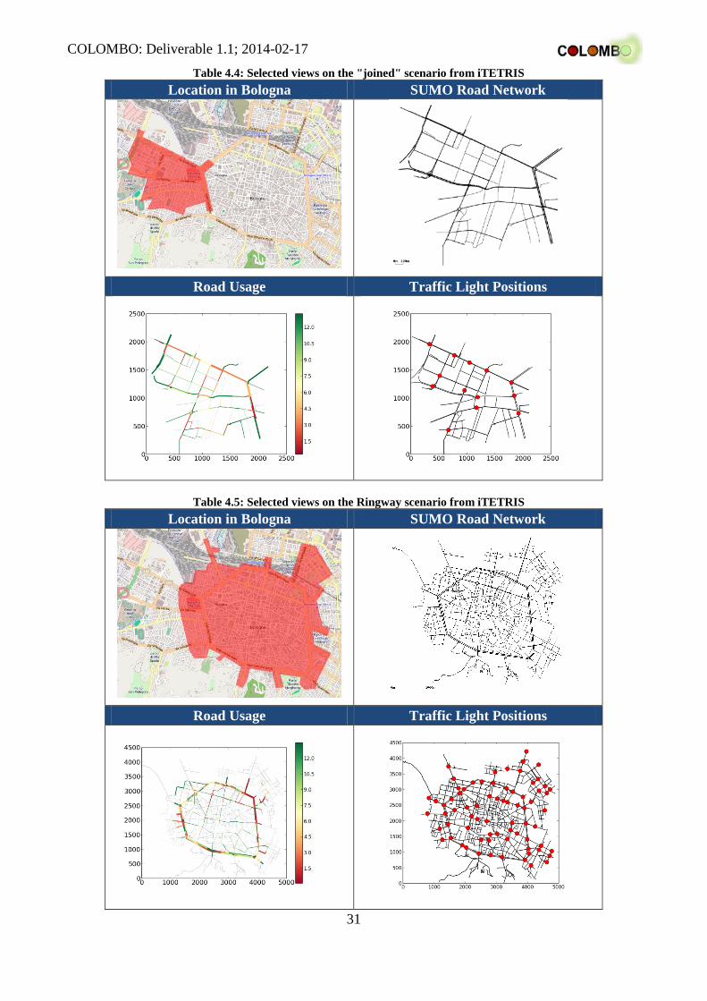
The given data included representations of two smaller parts of the network, namely the areas around the “Andrea Costa” and the “Pasubio” roads, as input files for the commercial microscopic traffic simulation Vissim, a product of PTV AG. Three larger scenarios were given as input files for VISUM, a macroscopic traffic model by PTV AG. Each of the scenarios included the demand for Bologna’s peak hour (8:00am – 9:00am). Additional data sets supported by the municipality of Bologna included positions of traffic lights, traffic light plans, inductive loop positions and measures and many others, the complete list can be found in the iTETRIS deliverable D3.2, “Traffic Modelling: ITS Algorithms” [iTETRIS D3.2, 2010]. A further scenario, “joined”, was implemented within iTETRIS by merging both Vissim scenarios.
Within iTETRIS, the files have been converted into SUMO, partially using newly developed tools, and adapted modified afterwards. An overview of this import process can be found in [iTETRIS D3.2, 2010]. Table 4.4 shows the resulting road networks in the context of the complete city.
The Bologna scenarios have some peculiarities:
1. Some roads are dedicated to public transport. Albeit passenger vehicles are prohibited, one can find them within the inductive loop measures.
2. Bologna uses the UTOPIA traffic light system (see also [COLOMBO D2.1, 2013]). UTOPIA is highly flexible – not only can phase durations be adapted to the current traffic situation, but also optional phases can be inserted or removed. As UTOPIA is proprietary and closed, it is hardly possible to replicate its algorithms within a simulation model. The generated simulations use the original phase plans supported by the municipality of Bologna. The scenario uses fixed-time phases, but the information about the variable phases’ minimum/maximum durations are stored in the scenarios’ traffic light descriptions.
3. The available data includes inductive loop measurements for a day where a football match took place, allowing to model the additional visitors demand.
4. Many of the roads within the inner city are unidirectional.
In their current state, the scenarios from iTETRIS have the following issues:
1. Multi-lane roundabouts are not properly simulated; the simulation cannot handle the real flow at multi-lane roundabouts yielding in unrealistic jams; the issue is currently under investigation (A.Costa, joined),
2. The demand is given for one hour only (all), 3. Public transport is not included (ringway), 4. Pedestrian crossings are not included (all), 5. No information about pedestrian or two-wheeled movements is available.

COLOMBO: Deliverable 1.1; 2014-02-17
30
Table 4.2: Selected views on the A. Costa scenario from iTETRIS Location in Bologna SUMO Road Network
Road Usage Traffic Light Positions
Table 4.3: Selected views on the Pasubio scenario from iTETRIS Location in Bologna SUMO Road Network
Road Usage Traffic Light Positions
COLOMBO: Deliverable 1.1; 2014-02-17
31
Table 4.4: Selected views on the "joined" scenario from iTETRIS Location in Bologna SUMO Road Network
Road Usage Traffic Light Positions
Table 4.5: Selected views on the Ringway scenario from iTETRIS Location in Bologna SUMO Road Network
Road Usage Traffic Light Positions

COLOMBO: Deliverable 1.1; 2014-02-17
32
IMTECH Scenarios: Assen/Netherlands
Table 4.6 shows as scenario the north of the city of Assen (Netherlands). This scenario was converted from a Vissim network and has large traffic streams going north-south and vice versa depending on the time of the day. This is because this network connects between highway on- and off-ramps to the north and the city centre to the south. The area itself is an industrial area, which leads to traffic turning at the intersections as well. The main policy goal for the network is to have a green wave in north-south direction while not causing too much waiting time and long queues for other traffic.
Figure 4.2: Location of Assen
The middle two intersections also have pedestrian and bike crossings that are part of the traffic light control plan. The original plans are semi-dynamic, the main direction has a fixed time green wave, while the other signal groups allow for some flexibility according to demand. In the scenario this is implemented as a completely fixed time plan that approximates the original plan in the best way possible. A problem with this is that the clearance and intergreen times between each signal group pair can be different. This means that the plan, even implemented as completely fixed time, will still be very complex. Therefore, the signal times included in the scenario use an average intergreen time. Later in the project it will be investigated if an interface between SUMO and the original controller can be made, so that the semi-dynamic behaviour can be simulated with the same controller as used in reality. When the interfacing is done the new control method Imflow can be used in this scenario too, which is a state of the art product released in 2011 and is also an adaptive controller like UTOPIA. This is because there are plans to upgrade the controllers in Assen to this new system.

COLOMBO: Deliverable 1.1; 2014-02-17
33
Table 4.6: Selected views on the Assen scenario Location in Assen SUMO Road Network
Road Usage Traffic Light Positions
IMTECH Scenarios: Pickering/ United Kingdom
Table 4.7 shows a scenario from Pickering, North Yorkshire, in the United Kingdom where left-hand driving is ruled.
Figure 4.3: Location of Pickering

COLOMBO: Deliverable 1.1; 2014-02-17
34
This scenario was originally made in Vissim, but is converted to SUMO for the COLOMBO project. Theoretically it should not make a difference for a traffic light controller whether traffic is right- or left-handed, but it is good to have a scenario with left-hand driving as well to be able to verify this. Another challenge on this network is the roundabout to the right. This intersection is not controlled, but can cause small traffic jams that spill back to the single intersection on the left. Therefore, this scenario is a good test case to see how a controller deals with spillback. On a more detailed level, the intersection also contains pedestrian crossings and has partial conflicts between right turning traffic and oncoming traffic that is going straight. The right turning traffic has to wait for a gap in the oncoming traffic before it can leave the intersection. This can again be challenging to the controller as this causes the saturation flow to vary with the turning percentage.
Table 4.7: Selected views on the Pickering scenario Location in Pickering SUMO Road Network
Road Usage Traffic Light Positions
ORINOKO Scenarios: Nuremberg/Germany
ORINOKO (“Operative Regionale Integrierte und Optimierte Korridorsteuerung”) was a national (German) project performed between 2004 and 2008, funded by the German Federal Ministry of Economics and Technology. The project objectives were to design and implement traffic management solutions for a city-wide traffic surveillance, quality assurance, and for traffic lights improvement. The city of Nuremberg was this project’s test site.

COLOMBO: Deliverable 1.1; 2014-02-17
35
Figure 4.4: Location of Nuremberg
One of ORINOKO’s sub-tasks the COLOMBO partner DLR was involved in was the simulative evaluation of daily switch plans – time tables that switch between previously defined traffic light programs – and their switching procedures. For this purpose, a set of simulation scenarios that represent selected parts of the city, all located around the fair trade centre, was implemented. The traffic lights definitions, including weekly switch time plans, were supplied and embedded in the scenarios. By now, a scenario covering a single intersection was made available to COLOMBO project partners. Others, including larger areas are being examined.
Table 4.8: Selected views on the K573 scenario from ORINOKO Location in Nuremberg SUMO Road Network
Road Usage Traffic Light Positions

COLOMBO: Deliverable 1.1; 2014-02-17
36
4.2.2 Scenario Comparison Table 4.9 lists basic object parameters and meta data of the scenarios that were made available within COLOMBO.
Table 4.9: Overview of the iTETRIS Scenarios Scenario Name Parameter / Meta Data A
. Cos
ta
Pasu
bio
join
ed
ring
way
K 5
73
Ass
en
Pick
erin
g
Network
Number of Nodes3 115 65 162 1209 32 153 107 Number of Traffic lights 7 8 13 73 1 5 1 Number of Edges 182 111 271 2208 58 193 110 “Width” [m] ~1817 ~1827 ~2164 ~4891 ~3286 ~640 ~1245 “Height” [m] ~1557 ~1339 ~2123 ~4216 ~4142 ~1206 ~414 Demand Begin Time 8:00 8:00 8:00 8:00 0:00 End Time 9:00 9:00 9:00 9:00 24:00 Vehicle Number 8888 8681 11079 19987 26004 4870 3394 Scenario Origin iTETRIS ORINOKO IMTECH
Enhancement in COLOMBO
Validation of the simulation, corrections and update of the road network (e.g. number of lanes adapted, wrong streets remove), traffic demand updated
Traffic demand and traffic network
Trafic demand, network and infrastructure converted into SUMO format
The scenarios differ in size and complexity, ranging from single intersection scenarios up to complete inner city rings. The scenarios cover areas with peculiar characteristics, such as dedicated bus lanes and edges or weekly switch time plans. This heterogeneity should allow to investigate whether the developed solutions are working as wished in complex situations. Nonetheless, further scenarios would be of benefit.
In their current state, no scenario regards pedestrians or bicyclists. After implementing the according functionalities into SUMO, performed in COLOMBO’s task 5.2, “Traffic Lights for Pedestrians and Bicycles”, the scenarios have to be updated by incorporating the infrastructure used by these groups as well as the according demands.
In Table 4.10, the scenarios are put against the requirements initially formulated in section 4.1. One may note that one certain requirement is not covered sufficiently, namely demands replicating situations. This information was not available in the initial scenarios and has to be computed. A previously implemented attempt to calibrate the demand to given inductive loop measures is being applied, but the results are not yet satisfactory.
3 Please note the number of nodes and the number of edges is influenced by the road network representation. In SUMO, an edge has a constant number of lanes and the lanes have constant widths and maximum velocities along their complete length. As a result, additional lanes in front of intersections have to be modelled using additional edges, increasing the edge number. As an edge connects two nodes in SUMO, this also increases the number of nodes.

COLOMBO: Deliverable 1.1; 2014-02-17
37
Table 4.10: Fulfilling the requirements by scenario
iTE
TR
IS/A
. Cos
ta
iTE
TR
IS/P
asub
io
iTE
TR
IS/jo
ined
iTE
TR
IS/r
ingw
ay
OR
INO
KO
/K 5
73
IMT
EC
H/A
ssen
IMT
EC
H/P
icke
ring
single intersection: both controlled and uncontrolled intersections must be modelled
x x x x x x
single intersection: three arms and four arms crossings
x x x x
multiple intersections (corridor and net) : both controlled and uncontrolled intersections must be modelled
x x x x x x
net: a scenario with at least five traffic lights x x x x x roads should be long enough to cover the communication range
x x x x x x x
should be based on real-world data x x x x x x x
different traffic amounts / situations such as workdays, peak hour, weekend, football match
different vehicle types x x x
4.3 Synthetic Scenarios The biggest problem in defining synthetic scenarios gets already visible when looking at a simple intersection: the large number of possible configurations. We see the following variables:
• per edge • number of lanes: natural (integer) numbers between 1 and 10 • allowed velocity: {30, 40, 50, 60, 70 km/h} • angle at intersection: real number between {-45, 45} in ° • additional lanes at the end of the road: between 0 and 5
• distance of begin to the intersection: real number in meters • direction {left, right}
• per lane • allowed driving directions: {left, straight, right}* • special rules: {none, right-turning is always allowed, partial conflicts}* • allowed vehicle classes {all, hov, public transport, bicycles, pedestrians} • width: real number in meters
• central reservation (width) • pedestrian crossings (width)
Where * denotes that the variable is not completely free, e.g. in case of driving directions, crosses of paths should not occur and partial conflicts only occur between left turning traffic an on-going straight traffic or between pedestrians/bikes and right turning traffic.
The demand at a single intersection is characterised by a variety of attributes. Different possibilities to store demand information, such as turning probabilities or O/D matrices. Extending the

COLOMBO: Deliverable 1.1; 2014-02-17
38
definitions of scenarios in RiLSA ([FGSV, 2010a]), one could obtain the following definition scheme:
• per incoming edge • time line of motorized demand: natural (integer) number of vehicles/h
• choosing a following direction {left, straight, right}, i.e., turning percentage (time line) • (time line of) percentage of heavy duty vehicles: floating point number between 0 % and
100 % • (time line of) percentage of bicycles: floating point number between 0 and 100 % • (time line of) percentage/number of special vehicles: natural (integer) number of vehicles • pedestrians (time line): natural (integer) number of pedestrians/h
One can easily see that – even if a discretization for the few attributes that are defined using floating point numbers would be chosen – the number of possible configurations is huge. As a result, the major issue when developing synthetic scenarios is not to realize them technically, but rather to choose the meaningful ones. Advices that point to meaningful scenarios are not known. The single intersection examples used within the publications evaluated and presented within the state-of-the-art section (Section 2.6) differ in the number of an edge’s lanes, the directions a vehicle may take when being at a certain lane, as well as in the number of additional lanes in front of an intersection. A motivation for choosing a certain parameter set is only seldom given.
In addition, a specific algorithm that shall be benchmarked using these scenarios may be sensitive to certain road network attributes. When choosing road networks a priori, certain combinations that could show the algorithm’s peculiarities would be probably missing.
Therefore, instead of choosing a set of abstract scenarios to implement in COLOMBO, a tool set for building synthetic scenarios was designed and implemented. As described in the following sections, the tool allows to configure both, the road network and the demand along multiple dimensions. Within evaluations of traffic management applications often the demand of two crossing flows is iterated in equidistant steps and the PI for each combination plotted, as shown in Figure 4.5 for the average waiting steps (= time) of a platoon forming vs. a static policy. The implemented scenario generator (SG) extends this approach to road networks. As a result, the SG allows to iterate not only along the demands, but also the road network’s attributes, allowing to take these into account during the evaluation of a traffic management application. This feature will be used in later steps of the COLOMBO project, mainly within the development of the “Traffic Light Algorithms Evaluation Schema”, performed in Task 5.3.
Figure 4.5: Example of evaluating a traffic light by iterating over two flow demands [COLOMBO D2.1, 2013]
The following sub-sections describe the SG in a larger detail. At first, the possibilities to build a large variety of road networks are described. Then, it is shown how demands can be generated that
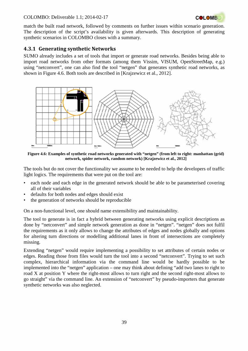
COLOMBO: Deliverable 1.1; 2014-02-17
39
match the built road network, followed by comments on further issues within scenario generation. The description of the script’s availability is given afterwards. This description of generating synthetic scenarios in COLOMBO closes with a summary.
4.3.1 Generating synthetic Networks SUMO already includes a set of tools that import or generate road networks. Besides being able to import road networks from other formats (among them Vissim, VISUM, OpenStreetMap, e.g.) using “netconvert”, one can also find the tool “netgen” that generates synthetic road networks, as shown in Figure 4.6. Both tools are described in [Krajzewicz et al., 2012].
Figure 4.6: Examples of synthetic road networks generated with “netgen” (from left to right: manhattan (grid)
network, spider network, random network) [Krajzewicz et al., 2012]
The tools but do not cover the functionality we assume to be needed to help the developers of traffic light logics. The requirements that were put on the tool are:
• each node and each edge in the generated network should be able to be parameterised covering all of their variables
• defaults for both nodes and edges should exist • the generation of networks should be reproducible
On a non-functional level, one should name extensibility and maintainability.
The tool to generate is in fact a hybrid between generating networks using explicit descriptions as done by “netconvert” and simple network generation as done in “netgen”. “netgen” does not fulfil the requirements as it only allows to change the attributes of edges and nodes globally and options for altering turn directions or modelling additional lanes in front of intersections are completely missing.
Extending “netgen” would require implementing a possibility to set attributes of certain nodes or edges. Reading those from files would turn the tool into a second “netconvert”. Trying to set such complex, hierarchical information via the command line would be hardly possible to be implemented into the “netgen” application – one may think about defining “add two lanes to right to road X at position Y where the right-most allows to turn right and the second right-most allows to go straight” via the command line. An extension of “netconvert” by pseudo-importers that generate synthetic networks was also neglected.

COLOMBO: Deliverable 1.1; 2014-02-17
40
The most flexible way to realise the generation of synthetic scenarios was to implement a Python-API to “netconvert”. The script builds networks as following:
1. set up defaults for nodes / edges 2. build an internal network representation: use an algorithm to put default-typed nodes on a plane
and connect them using default-typed edges 3. override certain nodes’ or edges’ variables or apply other operations on the internal network
representation 4. Write the internal network representation to files readable by “netconvert” 5. Execute “netconvert“ to build the network
The algorithm that puts nodes on the plane resembles the network types; at the current time, the following types are implemented: straight, cross, corridor, grid. Other described algorithms, such as Voronoi networks [Härri, Filali, Bonnet, 2009], or spider and random networks as generated by “netgen” are not implemented.
Figure 4.7: The default grid network (left: complete network, right: focus on a single intersection)
We want to demonstrate this tool capability. The tool is integrated into SUMO’s tool suite. After setting the paths to SUMO libraries via the environment variable PYTHONPATH and starting Python, we may generate a large grid network, as shown in Figure 4.7, using the following commands4: >>> import sumolib.net.generator.grid as generator >>> net = generator.grid() >>> net.build()
Single Intersection Configurations
The script is capable to generate a large variety of road networks. Table 4.11 shows some single intersection configurations, based on examples from literature (scientific papers and guidelines), and including the code needed to generate them. It shows how a single intersection can be influenced. Please note that the pedestrian crossings are still missing in the networks, see also Section 5.1.
4 Please note that the scenario generator is currently in a development phase and that it’s functions and usage may change therefore

COLOMBO: Deliverable 1.1; 2014-02-17
41
Table 4.11: Example Road networks generated using the Scenario Generator Source Original Image As Generated
[Yan, Dridi, El Moudni, 2012]
>>> import sumolib.net.generator.cross as generator >>> from sumolib.net.generator.network import * >>> defaultEdge = Edge(numLanes=3, maxSpeed=13.89, \ lanes=[Lane(dirs="rs"), Lane(dirs="s"), Lane(dirs="l")]) >>> net = generator.cross(None, defaultEdge) >>> net.build()
[FGSV, 2010b], example 1
>>> import sumolib.net.generator.cross as generator >>> from sumolib.net.generator.network import * >>> defaultEdge = Edge(numLanes=1, maxSpeed=13.89) >>> defaultEdge.addSplit(100, 1) >>> defaultEdge.lanes = [Lane(dirs="rs"), Lane(dirs="l")] >>> net = generator.cross(None, defaultEdge) >>> net.build()
[FGSV, 2010b], example 35
>>> import sumolib.net.generator.cross as generator >>> from sumolib.net.generator.network import * >>> defaultEdge = Edge(numLanes=1, maxSpeed=13.89) >>> defaultEdge.addSplit(100, 1) >>> defaultEdge.lanes = [Lane(dirs="rs"), Lane(dirs="l")] >>> net = generator.cross(None, defaultEdge) >>> net.addEdge(Edge("1/0_to_1/1", net.getNode("1/0"), net.getNode("1/1"), \ numLanes=3, maxSpeed=13.89, \ lanes=[Lane(dirs="r"), Lane(dirs="s"), Lane(dirs="l")])) >>> net.build()
5 One may miss the second example from RiLSA; it is currently not possible to build it as it contains a central reservation what is not supported by “netconvert“

COLOMBO: Deliverable 1.1; 2014-02-17
42
[FGSV, 2010b], example 4
>>> import sumolib.net.generator.cross as generator >>> from sumolib.net.generator.network import * >>> defaultEdge = Edge(numLanes=1, maxSpeed=13.89) >>> defaultEdge.addSplit(100, 1) >>> defaultEdge.lanes = [Lane(dirs="rs"), Lane(dirs="l")] >>> net = generator.cross(None, defaultEdge) >>> net.addEdge(Edge("0/1_to_1/1", net.getNode("0/1"), net.getNode("1/1"), \ numLanes=3, maxSpeed=13.89, \ lanes=[Lane(dirs="r"), Lane(dirs="s"), Lane(dirs="l")])) >>> net.build()
And, of course, it is possible to quickly iterate over the values of a road network: >>> import sumolib.net.generator.cross as generator >>> for i in range(1, 5): >>> defaultEdge = Edge(numLanes=i, maxSpeed=13.89) >>> net = generator.cross(defaultEdge) >>> net.build("net_with_%s_lanes.net.xml" % i)
The road networks generated by this script are shown in Figure 4.8.
Figure 4.8: Intersections obtained by iterating over the edges’ lane numbers (from left to right, top to bottom)

COLOMBO: Deliverable 1.1; 2014-02-17
43
Configurations of Multi-Node Networks
More complex networks can be built using other “generators” than the “cross” generator used in the examples above. Besides “cross” that build a single intersection, the following generators currently exist: “straight”, “corridor”, and “grid”. All align the built nodes in a matrix, where corridor and straight have only one horizontal path. The nodes are named by using their x- and y-position within this matrix. Both start at zero. Horizontally they are built from right to left, vertically from bottom to top. As shown in Figure 4.9, node “1/2” is the second from left to right and third from bottom to top, e.g. This clear naming eases the later definition of the demand (see Section 4.3.2) and additionally allows to apply filters to the nodes’ positions or other attributes.
Figure 4.9: The layout of a grid network as generated by the SG
Both nodes and edges are built using the defaults set before the network generator is started. This means that the network’s edges and nodes can be globally altered using the same methods as shown in Table 4.11. After running the generator, the building script can explicitly change an existing edge as shown in the RiLSA4 example in Table 4.11. Edges can be added to as well as removed from the network.
Reproducibility
If a certain generated road networks is used for a research, the small number of needed commands to define it should allow to include its definition in the according report. Of course, a programming language code is not a very well readable kind of definition. A description language could be defined, but this is assumed to be out of scope of this deliverable.
It should be also noted that the SG is currently only working with SUMO. The network descriptions SG generates are native to SUMO’s network building module “netconvert”. It is assumed that extending SG by other export facilities should be easily possible. In addition, “netconvert” allows exporting road networks to MATsim6 and OpenDRIVE7 and could also be extended by other export possibilities. But even if other simulations’ road descriptions could be generated, the resulting networks would differ. This is due to the fact that “netconvert” employs heuristics where certain
6 http://www.matsim.org/ 7 http://www.opendrive.org/

COLOMBO: Deliverable 1.1; 2014-02-17
44
information is missing and SG does not describe the network completely in all cases, see [Krajzewicz et al., 2005]. This means that for replicating a network exactly, not only the descriptions generated by SG, but also algorithms implemented in “netconvert” must be known.
4.3.2 Generating synthetic Demands In contrary to real-world scenarios, where the demand is too complex to be described in an abstract way, the demand in synthetic scenarios should be able to be described using a small number of parameters, mainly for making it replicable. The SG defines the demand by a set of “streams”. Each stream consists of:
• an ID: used to name the generated vehicles • validFrom: the begin of the time interval covered by this model • validUntil: the end of the time interval covered by this model • models for:
• the number of vehicles: determines the number of vehicles (the flow) • the depart edge: determines the edge a vehicle begins its route at • the destination edge: determines the edge a vehicle ends its route at • the vehicle type: determines the ID of a generated vehicle’s type
The following models are currently implemented for the depart edges, the destination edge, and the vehicle type:
• string: the given string is directly used • dict: a map containing the probabilities and the according elements
A very basic example for a stream that uses both models is: >>> demand = Demand() >>> demand.addStream(Stream(None, None, None, 1000, "from", "to", { .2:"hdv", .8:"passenger"})) >>> demand.build(0, 7200)
This builds a static flow of 1000 veh/h that start at edge “from” and end their route at edge “to”. To 20 % of the vehicles the type “hdv” is assigned, while 80 % of the vehicles will have the type “passenger”. This is done by interpreting the parameter used in the above script example as following:
• ID=None: this is a special value for IDs; if no value (“None”) is given, the IDs will be automatically computed using the scheme <FROM_EDGE>_to_<TO_EDGE>_<RUNNING_NUMBER> (where <FROM_EDGE> is the edge the vehicle starts at, <TO_EDGE> is the edge it ends at and <RUNNING_NUMBER> is the number of vehicle within this stream)
• validFrom=None: None denotes here that no time restrictions are valid for this model • validUntil=None: None denotes here that no time restrictions are valid for this model • number of vehicles=1000: 1000 veh / h in this case (used directly) • depart edge=”from”: all vehicles will be inserted into the road network at edge “from” • destination edge=”to”: all vehicles will leave the road network at edge “to” • vehicle type=dict: 20% of the vehicles will have the type “hdv” while 80 % will be of the type
“passenger”
One may note that the number of the vehicles to generate is given an integer value. Iterations along different demands as shown in Figure 4.5 can be easily realised by iterating this value accordingly. But when adaptive traffic lights algorithms are investigated, a time-variable demand is needed to determine the algorithm’s responsiveness to changes in the controlled flows. For this reason, the vehicle number to be inserted can be defined using a larger variety of models:

COLOMBO: Deliverable 1.1; 2014-02-17
45
• integer: the given integer is directly interpreted as vehicle flow in vehs/h; the departure time is chosen randomly from the given time span, respecting the probability dictated by the vehicle flow
• LinearChange: this model is interpreted as a linear change of the demand between two given flow values within a given time interval. It is assumed to be used to measure how fast an algorithm adapts to changes in the demand. The parameters are:
• beginFlow: the flow at beginTime • endFlow: the flow at endTime • beginTime: the begin of the time interval covered by this model • endTime: the end of the time interval covered by this model
• WaveComposition: In [Sohr, Wagner, Brockfeld, 2009], a method for decomposing time lines of velocities was presented. The “WaveComposition” model uses this approach to model time-varying demands using trigonometric functions as components. These components’ values at a given time t are summed to obtain f(t), the flow at this time:
∑=
++++=N
ioboaftf
1iiiiii0 ))(tsin())(tsin()( ϖϖ
where 0f is an average flow level
iΦ= πϖ 2i with iΦ being the frequency of the component
iba ,i are amplitudes of the component
io are time offsets of the component
Figure 4.10 shows the results of using these models to describe flows. As one can see, the “WaveComposition” model allows to model daily flow time lines. The flows shown in Figure 4.10 were defined as following:
static: >>> demand = Demand() >>> demand.addStream(Stream(None, None, None, 800, "from", "to", "passenger"))
linear increase: >>> demand = Demand() >>> demand.addStream(Stream(None, 0, 39600, 400, "from", "to", "passenger")) >>> demand.addStream(Stream(None, 39600, 46800, LinearChange(400, 1200, 39600, 46800), \ "from", "to", "passenger")) >>> demand.addStream(Stream(None, 46800, 86400, 1200, "from", "to", "passenger"))
wave composition: >>> demand = Demand() >>> demand.addStream(Stream(None, None, None, WaveComposition(800, [ [400, 0, .000025, 14400], [200, 0, .00001, 14400] ]), "from", "to", "passenger"))

COLOMBO: Deliverable 1.1; 2014-02-17
46
Figure 4.10: Possibilities to define demands within the SG using different models
4.3.3 Further Notes As the SG knows the IDs of all edges at the generated network’s boundaries, it is easily possible to iterate them and build demands that start at those. This allows to apply a demand to all of a generated network’s feeding edges automatically.
Testing whether the implemented models improve the possibilities to evaluate traffic light algorithms is performed in sub-sequent steps of the projects and will be reported in later deliverables.
Besides the road network and the demand, a scenario usually includes further structures, such as inductive loops, bus stops, RSUs, etc. At the current time, such additional structure may be automatically generated for a given road network, albeit using additional, dedicated scripts. SG will be extended by this functionality.
4.3.4 Deployment
State
Albeit SG’s basic functionality as described is implemented, the currently available version should be stated preliminary (“alpha”). Extensions to both network generators as well as to the demand models are assumed to be needed. Currently, the SG is rather the API only and its execution requires programming skills in the Python programming language.
Availability
The functionality of SG is currently included in the COLOMBO-branch of SUMO, accessible by third parties. It will be moved to SUMO’s official branch as soon as a stable state has been reached and the documentation (see below) is completed.
System Requirements
Being written in Python 2.7.x, the script can be executed on all platforms for which Python is available. That is true for all common platforms, including MS Windows, Linux, and Mac OS. The script directly parses the entries step-by-step, so that no limits arising from memory consumption should be assumed.
static with linear increase wave composistion

COLOMBO: Deliverable 1.1; 2014-02-17
47
User Documentation
Being in an alpha development phase, the SG currently lacks a user documentation.
Tests
Tests set up for being executed every night as a part of SUMO's test suite assure the tool behaves correctly. These tests are currently stored in the COLOMBO-branch of SUMO and will be included in SUMO's official release together with the script itself. Currently, the tool is tested for:
• building single intersections, including the examples from Table 4.11 (5 tests) • building networks using the different generators (corridor, grid, cross, straight) defaults (4 tests)

COLOMBO: Deliverable 1.1; 2014-02-17
48
5 Needed Extensions In the following, the extensions needed to be done on the COLOMBO components are described. They partially extend the requirements formulated in [COLOMBO D5.1, 2013]. A brief introduction of each component can be found in section 4.1.
5.1 SUMO
Pedestrians and Bicycles
COLOMBO puts a large focus on taking pedestrians and bicycles into account. An own task, Task 5.2, “Traffic Lights for Pedestrians and Bicycles”, is dedicated to extending SUMO by according models. Regarding pedestrians, the extensions should resemble pedestrians crossing the road as well as moving along the road. The inclusion of pedestrian crossings into SUMO road networks highly increases the complexity of SUMO’s intersection model. Therefore, different modelling attempts are tested and compared. Despite the implementation of pedestrian traffic lights, crossings, and pathways within the simulation, the network importers as well as the scenario generator presented in this deliverable must be extended so that these structures can be imported or added to the generated scenarios using proper heuristics.
Similar extensions are needed to incorporate bicycles on dedicated lanes, but additional effort is to be put into modelling of a shared use of lanes by both cars and bicycles. The extensions on SUMO performed to simulate pedestrians and bicycles will be reported in COLOMBO’s deliverable 5.2, “Traffic Simulation Extensions”.
Simulation Improvements
Taking the opportunity to explicitly work on traffic light evaluations, SUMO’s quality in representing the behaviour at traffic lights should be revalidated. This should at least include measurements of macroscopic properties, such as the saturation flow. Microscopic trajectories of vehicles may as well be investigated, mainly in conjunction with work performed in Task 4.3 (“Simulation and Optimisation”) where an emission-optimal driver behaviour shall be developed.
Figure 5.1: The same intersection, once not regarding pedestrian crossing areas (left) and once with halting
lines that regard the area of pedestrian crossings (right)
Some first tests proved the assumption that neglecting pedestrian crossings changes the performance of an intersection dramatically as the additional standing place the areas of pedestrian crossings offer is missing. In the following, the first examples scenario from RiLSA ([FGSV, 2010a]) is used. The left side of Figure 5.1 shows the scenarios modelled in the usual way in SUMO – without pedestrian crossings. On the right side of the Figure, the same scenario with

COLOMBO: Deliverable 1.1; 2014-02-17
49
additional edge offsets of 5 m to the intersection is given. These offsets model the halting line at the intersection before a pedestrian crossing. One can already see, that only one left-moving vehicle can enter the network if no pedestrian crossing area is modelled, two if it is given.
Given the same demand, the original scenarios needs 4348 steps to let the modelled flow pass the scenario completely (all vehicles have entered and left the scenario) while the scenario with additional offsets needs 3699 steps. The vehicles insertion times cover one hour (3600 s). As supposed initially, this change is resulting from the additional space left-moving vehicles have on the intersection. The left hand side of Figure 5.2 shows that the jam at the left lane of the stream coming from south is getting longer continuously (dark, broken line) and the average speed sinks accordingly. This is not the case as soon as the additional place vehicle may use to pass the intersection is available, as shown on the right hand side of Figure 5.2.
Figure 5.2: Traffic conditions at the edges coming from north (nm*, light blue) and south (sm*, dark blue); the right lanes are shown using solid, left lanes using broken lines; top: the average jam length over time, bottom:
the average speed over time; left: no pedestrian crossings areas, right: with pedestrian crossing areas
Over the past years, SUMO was extended by different sub-models that realize certain outputs, model passing an intersection by following the leader, let vehicles keep intersections free so that opposite traffic can pass, realize simulation steps below 1 s, etc. Even though these extensions increased SUMO’s quality in reproducing traffic and opened it for a wider range of applications, they negatively influenced the simulation’s execution speed. When working with simple scenarios, such as single cross intersections, some of these sub-models are not necessary. It should be investigated, whether it is possible to disable some of these features at purpose.
Evaluation of traffic lights should always use more than one simulation run for a single setting to obtain statistically valid results. Currently, SUMO’s randomness only affects the car-following model of longitudinal progress of single cars, making them behave slightly different as soon as they are on the road. But the departure time of vehicles should be stochastic, too. The planned extension is meant to vary the given insertion (departure) time of vehicles by a user-defined amount in a stochastic way.

COLOMBO: Deliverable 1.1; 2014-02-17
50
Finally, the simulation model should be extended by special treatments of multi-lane roundabouts, as unrealistic jams arise at such places.
Computation of Performance Indicators
In chapter 3 of this document, the performance indicators used by COLOMBO were listed. In further development steps, it should be assured that they are computable by SUMO. Most of the network-wide PIs can already be computed as defined, but intersections PIs need a revalidation.
5.2 ns-3 The full support of WiFi-Direct in iTETRIS is not required for the purpose of the COLOMBO project. We abstracted the support of WiFi-Direct with three new extensions in ns-3. First, we added the support of the ETSI ITS G5C band at 5.5GHz – 5.7GHz. In the COLOMBO scenarios, WiFi-Direct is assumed to operate in such frequency band (see Figure 5.3) first for proximity reasons with the C2X ETSI ITS G5A and ITS-G5B bands and also for flexibility reasons between ITS services, which could be interchangeably exchanged on C2X on ITS G5B or WiFi-Direct on ITS G5C transparently to the traffic surveillance application.
Figure 5.3: Spectrum Allocation at 5GHz - ITS G5, WiFi 5, and WiFi-Direct
WiFi-Direct operates in the IEEE 802.11 ad-hoc mode, which ns-3 already supports. However, the P2P Discovery procedure is based on a cognitive principle, where the IEEE 802.11 scanning phase is enhanced with a listen-search phase to converge to a rendezvous channel between P2P devices. In ns-3, the scanning functions are part of the ns-3::station_manager, which role is to detect beacons/probe-requests and manage the IBSS. A new ns-3::wifi-direct-station_manager, based on the ns-3::vehicle-station_manager, has been added to the ns-3 stack, with a ns3::wifi-direct-scan_manager handling the enhanced functionalities required for WiFi P2P discovery.
The P2P Group Management is not integrated in ns-3 directly but rather at the application module in order to leave more control to the COLOMBO applications to dynamically join/leave groups based on traffic surveillance requirements. The last extension consists of a ns3::iTETRIS_Service Provider (SP) and a ns3::iTETRIS_Service Consumer (SC) applications. Both SP and SC applications are not tightly connected to a particular access technology (WiFi-Direct, DSRC) or protocol stack (IPv6, C2X), but we linked to WiFi-Direct C2X Stack by default (see Figure 5.4).

COLOMBO: Deliverable 1.1; 2014-02-17
51
Figure 5.4: ns-3 extensions for COLOMBO (in red) - WiFi-Direct support, Service Provider (SP), Service Consumer (SC) as well as C2C Stack on WiFi-Direct. The WiFi-Direct Station Manager implements two new
WiFi-Direct P2P Discovery (Listen/Search phases)
5.3 iCS A major innovation in COLOMBO scenarios is related to pedestrians. They may assist in traffic surveillance, first from their relatively static pace compared to vehicles, but also as they may carry a smartphone, which could interact with vehicles. The iCS implements a station/application manager, which role is to keep track of the number of SUMO vehicles integrated in iTETRIS, the number of vehicles equipped with particular communication interfaces (DSRC, UMTS etc..), and the number of vehicles with a given application. This leaves a large degree of freedom for iTETRIS developers to test their applications in various penetration conditions (see Figure 5.5).
Figure 5.5: iCS Station/Application Manager in iTETRIS
In COLOMBO, the joint availability of smartphones and pedestrians requires the iCS to be extended. Considering vehicles at first, the iCS needs to be able to model a gradual penetration rate of smartphones available either from drivers or passengers. It also has to include two new communication interfaces, namely WiFi-Direct and Bluetooth. Second, pedestrians are now available from SUMO and should be included, with a gradual penetration rate similarly to vehicles. Pedestrians may also experience a gradual penetration rate of smartphones. And last but not least, smartphones may not have all interfaces available (pedestrian might not wish to provide all interfaces, e.g.WiFi-Direct, DSRC, etc.., for energy-saving issues). As such, a gradual penetration of access technologies in smartphones should be included in the station manager of the iCS. Figure 5.6 depicts such required extensions by the iCS.

COLOMBO: Deliverable 1.1; 2014-02-17
52
Figure 5.6: Extension of the iCS for COLOMBO, where a gradual penetration rate of pedestrian, PDA, and
technologies (WiFi-Direct and Bluetooth) must also be considered
Similarly, RSU must also support alternate technologies. In iTETRIS, the available technologies for RSU stations in the iCS station manager is restricted to C2X. This should be extended to support also WiFi-Direct and Bluetooth, so that, RSU may also participate to traffic surveillance on the one hand and on the other hand it may receive traffic reports from WiFi-Direct-equipped smartphones.
All these new extensions should be available in the iCS scenarios in XML format, similarly to what currently exist for pure C2X equipped vehicles in iTETRIS.
The iCS plays the role of interface between the Application module and SUMO or ns-3. The Application module may require actions to be conducted by SUMO or ns3 by invoking ‘Subscriptions’ as illustrated on Figure 5.7.
Figure 5.7: iCS's subscription scheme
When designing traffic surveillance algorithms in the Application module, more than mobility or the reception/loss of packets is required to observe, form groups and fusion traffic data. Communication facilities are not reachable by the iCS in the iTETRIS platform and key channel statistics or received packet statistics required for data fusion, such as channel load, RCPI or RSNI remain in ns-3. This implies for iTETRIS to implement data fusion algorithm in ns-3, but COLOMBO requires it to be done in the Application module. Accordingly, the iCS subscriptions should be extended to be able to provide low-layers channel metrics to the Application module. Also, more flexibility in the technology selection should be allowed and as such, the communication facilities should also become reachable by the Application module through the iCS.
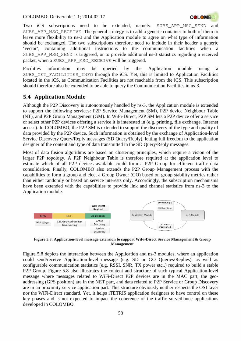
COLOMBO: Deliverable 1.1; 2014-02-17
53
Two iCS subscriptions need to be extended, namely: SUBS_APP_MSG_SEND and SUBS_APP_MSG_RECEIVE. The general strategy is to add a generic container to both of them to leave more flexibility to ns-3 and the Application module to agree on what type of information should be exchanged. The two subscriptions therefore need to include in their header a generic ‘vector’, containing additional instructions to the communication facilities when a SUBS_APP_MSG_SEND is triggered, or to provide additional ns-3 statistics regarding a received packet, when a SUBS_APP_MSG_RECEIVE will be triggered.
Facilities information may be queried by the Application module using a SUBS_GET_FACILITIES_INFO through the iCS. Yet, this is limited to Application Facilities located in the iCS, as Communication Facilities are not reachable from the iCS. This subscription should therefore also be extended to be able to query the Communication Facilities in ns-3.
5.4 Application Module Although the P2P Discovery is autonomously handled by ns-3, the Application module is extended to support the following services: P2P Service Management (SM), P2P device Neighbour Table (NT), and P2P Group Management (GM). In WiFi-Direct, P2P SM lets a P2P device offer a service or select other P2P devices offering a service it is interested in (e.g. printing, file exchange, Internet access). In COLOMBO, the P2P SM is extended to support the discovery of the type and quality of data provided by the P2P device. Such information is obtained by the exchange of Application-level Service Discovery Query/Reply messages (SD Query/Reply), letting full freedom to the application designer of the content and type of data transmitted in the SD Query/Reply messages.
Most of data fusion algorithms are based on clustering principles, which require a vision of the larger P2P topology. A P2P Neighbour Table is therefore required at the application level to estimate which of all P2P devices available could form a P2P Group for efficient traffic data consolidation. Finally, COLOMBO also extends the P2P Group Management process with the capabilities to form a group and elect a Group Owner (GO) based on group stability metrics rather than either randomly or based on service interests only. Accordingly, the subscription mechanisms have been extended with the capabilities to provide link and channel statistics from ns-3 to the Application module.
Figure 5.8: Application-level message extension to support WiFi-Direct Service Management & Group
Management
Figure 5.8 depicts the interaction between the Application and ns-3 modules, where an application could send/receive Application-level message (e.g. SD or GO Queries/Replies), as well as configurable communication statistics (e.g. RSSI, SNR, TX power etc..) required to build a stable P2P Group. Figure 5.8 also illustrates the content and structure of such typical Application-level message where messages related to WiFi-Direct P2P devices are in the MAC part, the geo-addressing (GPS position) are in the NET part, and data related to P2P Service or Group Discovery are in an proximity-service application part. This structure obviously neither respects the OSI layer nor the WiFi-Direct standard. Yet, it helps iTETRIS application designers to have control on these key phases and is not expected to impact the coherence of the traffic surveillance applications developed in COLOMBO.

COLOMBO: Deliverable 1.1; 2014-02-17
54

COLOMBO: Deliverable 1.1; 2014-02-17
55
6 Summary COLOMBO’s Task 1.1 should deliver a set of scenarios that can be used during the development of the traffic management applications in subsequent tasks of the project. This document should present the scenarios as well as additional requirements to the involved simulation applications.
The performed work was extended towards delivering a complete evaluation schema. For this reason, this document starts with a review of the state of the art in evaluating traffic management applications, focussing on traffic lights evaluation. A literature study performed in this context shows that up to date, the results of such evaluations can be hardly compared, as neither common – or well-defined – scenarios nor performance indicators are used.
To improve the comparability of the solutions developed in COLOMBO, the performance indicators to use within the project were defined, first. They are based on prior work done within iTETRIS, an earlier project co-funded by the European Commission. The performance indicators defined in iTETRIS were revisited and a new class of PIs, namely ones for measuring communication performance, was introduced. The work on performance indicators is meant to be continued by implementing functions into COLOMBO’s simulation system that allow computing them.
Different scenarios based on real world data were made available for the project partners. Trying to cover a large variety of scenarios, mainly scenarios set up in past projects have been re-used to avoid the effort needed to import and adapt new external data. The scenarios fulfil most of the requirements, but almost no scenario that covers a complete day exists and no special events are modelled, yet. Solving these issues needs two actions. At first, attempts to generate a time-dependent demand by using the given measurements from the real world should be tested. Secondly, the simulation model should be improved where needed to avoid the generation of unrealistic jams, as the case in multi-lane roundabouts. This is necessary, as otherwise the demand could not be calibrated to the inductive loop measures properly.
Instead of choosing a set of synthetic scenarios and implementing them, the decision to automatically generate such scenarios was taken, mainly for allowing investigations of the influence of the road network and of time-variable flows on adaptive traffic lights. The result of the design and implementation work is a scenario generation script capable to generate a large variety of synthetic scenarios that differ in the complexity of the overall road network, in the characteristics of the edges the road network consists of, and the demands that run through the networks.
The possibility to enumerate the network’s characteristics is assumed to be a major feature that is beyond the state-of-the-art in evaluation scenarios. It allows not only to examine an algorithm’s dependency on the flows, but also how certain intersection or network layouts influence the algorithm’s performance. The script is very light-weight and so easily extensible by further models for network layout or demand generation. The currently implemented features already allow a broader usage for the next tasks to be performed in COLOMBO than the usage of a pre-defined set of scenarios.
Besides adding models for new communication channels the used tool set is not yet capable to simulate, namely WiFi-Direct, the major extensions that have to be performed on the simulation suite regard the inclusion of pedestrians and bicyclists. As soon as models for these type of transport are, the scenarios used in COLOMBO will have to be updated by the according information.
COLOMBO: Deliverable 1.1; 2014-02-17
56
Appendix A – References [Akcelik, 2007] Akçelik, R.: Traffic models. on-line:
http://www.sidrasolutions.com/Resources/Models, last revised 15 July 2007, last accessed 30. October 2013.
[Austroads, 2006] Austroads: The use and application of microsimulation traffic models. Research Report AP-R286/06. Austroads, Australia. ISBN 1 921139 34 X. Available at: https://www.onlinepublications.austroads.com.au/items/AP-R286-06.
[Brackstone et al., 2012] Brackstone, M.; Montanino, M.; Daamen, W.; Buisson, C.; Punzo, V: Use, Calibration and Validation of Traffic Simulation Models in Practice: Results of a Web based Survey. In: Proc. of the 90th Transportation Research Board Annual Meeting. 2012, Paper 12-2606. TRB, Washington, D.C. U.S.A.
[Brackstone et al., 2014] Brackstone, M.; Punzo, V. (Eds.): Traffic Simulation: Case for Guidelines, JRC Science and Policy Report, EUR 26534 EN. European Commission, Luxembourg. 2014. ISBN 978-92-79-35578-3. 4. http://publications.jrc.ec.europa.eu/repository/handle/111111111/30680
[COLOMBO, 2012] COLOMBO consortium: Cooperative Self-Organizing System for low Carbon Mobility at low Penetration Rates – COLOMBO, Annex I – Description of Work, 2012.
[COLOMBO D5.1, 2013] COLOMBO consortium (publisher): COLOMBO project’s Deliverable D5.1: “Prototype of overall System Architecture and Definition of Interfaces”, July 2013.
[COLOMBO D4.1, 2013] COLOMBO consortium (publisher): COLOMBO project’s Deliverable D4.1: “Prototype of overall System Architecture and Definition of Interfaces”, October 2013.
[FESTA, 2008] FESTA consortium (publisher): Field opErational teSt supporT Action (FESTA) Handbook, Version 2. Deliverable D6.4, August 2008. http://www.its.leeds.ac.uk/festa/downloads/FESTA%20Handbook%20v2.pdf.
[FGSV, 2004] Forschungsgesellschaft für Straßen- und Verkehrswesen FGSV (publisher): HBS – Handbuch für die Bemessung von Straßenverkehrsanlagen, FGSV Verlag Köln, ISBN 3937356444, 2001.
[FGSV, 2006] FGSV (publisher): Hinweise zur mikroskopischen Verkehrsflusssimulation - Grundlagen und Anwendung [FGSV Nr. 388], FGSV Verlag Köln, ISBN 3-939715-11-5, 2006.
[FGSV, 2010a] FGSV (publisher): RiLSA: Richtlinien für Lichtsignalanlagen – Lichtzeichenanlagen für den Straßenverkehr, 2010.
[FGSV, 2010b] FGSV (publisher): Beispielsammlung zu den Richtlinien für Lichtsignalanlagen (RiLSA), 2010.
[FHWA, 2004] Federal Highway Administration FHWA (publisher): Traffic analysis toolbox volume III: guidelines for applying traffic microsimulation modelling software. FHWA-FRT-04-040. Washington, DC. Available at: http://ops.fhwa.dot.gov/trafficanalysistools/tat_vol3/vol3_guidelines.pdf.
[Härri, Filali, Bonnet, 2009] Härri, J.; Filali, F.; Bonnet, C.: Mobility models for vehicular ad hoc networks: a survey and taxonomy Communications Surveys & Tutorials, IEEE, 2009, pp. 19-41.
[iTETRIS, 2013] iTETRIS consortium (publisher): iTETRIS project web pages, online: http://www.ict-itetris.eu retrieved on 19 July 2013.
[iTETRIS D2.1, 2009] iTETRIS Consortium (publisher): iTETRIS Deliverable 2.1 – Co-operative traffic management strategies, August 2009.

COLOMBO: Deliverable 1.1; 2014-02-17
57
[iTETRIS D3.2, 2010] iTETRIS Consortium (publisher): iTETRIS Deliverable 3.2 –Traffic Modelling: ITS Algorithms, April 2010.
[Krajzewicz et al., 2005] Krajzewicz, D.; Hertkorn, G.; Ringel, J.; Wagner, P.: Preparation of Digital Maps for Traffic Simulation; Part 1: Approach and Algorithms, in Proceedings of the 3rd Industrial Simulation Conference 2005, pp. 285–290. In: EUROSIS-ETI. 3rd Industrial Simulation Conference 2005, Berlin (Germany), ISBN 90-77381-18-X.
[Krajzewicz et al., 2012] Krajzewicz, D.; Erdmann, J.; Behrisch, M.; Bieker, L.: Recent Development and Applications of SUMO - Simulation of Urban MObility, In: International Journal On Advances in Systems and Measurements, 5 (3&4):128-138, December 2012.
[Laval, n.d.] Laval, J.: Types of Simulation in Transportation. http://en.wikipedia.org/wiki/File:Simulation_Table.JPG, last accessed 30. October 2013.
[NGSIM, 2013] http://ngsim-community.org, last accessed: 30.10.2013.
[Rondinone et al., 2013] Rondinone, Michele; Maneros, Julen; Krajzewicz, Daniel; Bauza, Ramon; Cataldi, Pasquale; Hrizi, Fatma; Gozalvez, Javier; Kumar, Vineet; Röckl, Matthias; Lin, Lan; Lazaro, Oscar; Leguay, Jérémie; Haerri, Jérôme; Vaz, Sendoa; Lopez, Yoann; Sepulcre, Miguel; Wetterwald, Michelle; Blokpoel, Robbin and Cartolano, Fabio: ITETRIS: a modular simulation platform for the large scale evaluation of cooperative ITS applications. Simulation Modelling Practice and Theory. Elsevier. DOI: 10.1016/j.simpat.2013.01.007. ISSN 1569-190X.
[Sohr, Wagner, Brockfeld, 2009] Sohr, A.; Wagner, P.; Brockfeld, E.: Floating Car Data based travel time prediction with Lomb periodogram. Proceedings 16th World Congress on ITS. 16th World Congress on ITS, 21.-25. Sep. 2009, Sweden.
[Sommer et al., 2008] Sommer, Ch.; Yao, Z.; German, R.; Dressler, F.: On the Need for Bidirectional Coupling of Road Traffic Microsimulation and Network Simulation. MobilityModels’08, Hong Kong. http://www.ccs-labs.org/bib/sommer2008need/sommer2008need.pdf
[TfL, 2010] Transport for London: Traffic Modelling Guidelines, TfL Traffic Manager and Network Performance Best Practice. V3.0. Transport for London, London, UK. Available at: http://www.tfl.gov.uk/assets/downloads/traffic-modelling-guidelines.pdf.
[TRB, 2010] Transportation Research Board TRB (publisher): HCM2010 – Highway Capacity Manual, TRB, Washington D.C., 2010.
[VTRC, 2006] Virginia Transportation Research Council: Microscopic Simulation Model Calibration and Validation Handbook, Technical Report VTRC 07-CR6, Traffic Operations Laboratory, Center for Transportation Studies, University of Virginia, Park, B. and Won, J. Available at: http://www.virginiadot.org/vtrc/main/online_reports/pdf/07-cr6.pdf.
[Yan, Dridi, El Moudni, 2012] Yan, F.; Dridi, M.; El Moudni, A.: Combinatorial optimization algorithms for intelligent vehicle sequencing problem at an isolated intersection. In: International Journal of Combinatorial Optimization Problems and Informatics, ISSN 2007-1558, Volume: 3, Issue: 3, pp. 3-, 2012.