IC6501 - CS 2 MARKS WITH ANSWERS.doc

7/26/2019 IC6501 - CS 2 MARKS WITH ANSWERS.doc

http://slidepdf.com/reader/full/ic6501-cs-2-marks-with-answersdoc 1/41

S.A.ENGINEERING COLLEGE

(NBA Accredited, NAAC with ‘A’ grade & ISO 9001 !00"

Certi#ied I$%titti'$

A))r'*ed B+ AICE & A##i-iated t' A$$a $i*er%it+

/ESION BAN

S2ect C'de IC3401

S2ect Na5e CONROL S6SE7SAcade5ic 6ear !014 8 !013 ( O

6ear : Se5 III : ;

S5itted B+ .S.7ARGARE

e)art5e$t EEE

Sig$atre '# the Sta## Sig$atre '# the <O



S.A ENGINEERING COLLEGE

E=AR7EN O> ELECRICAL AN ELECRONICS ENGINEERING

;I SI ON

O BE A LEAER IN ENGINEERING ECAION,

RESEARC< AN O A==L6 <E NO?LEGE =RACICAL6

>OR <E BENE>I O> SOCIE6 GLOBALL6.

7I SSION

O SRI;E >OR =ROCI;E =ARNERS<I= BE?EEN

<E INSR6 AN <E INSIE.

O ENCORAGE AN >ACILIAE >ACL6,

RESEARC<ERS AN SENS O ?OR S6NERGISICALL6

ACROSS ISCI=LINE ?I<O BONRIES.

O >OSER LI>ELONG LEARNING AN E7=O?ER

SENS O BECO7E O7ORRO?’S LEAERS



=R O G R A7 7 E E C A I O N A L O B @ E C I ; E S

1. ' )r'*ide %tde$t% with %'$d #$da5e$ta- $'w -edge

c'5i$ed with g''d )ractica- 'rie$tati'$ %' a% t' ide$ti#+ a$d a))-+

their r'ad $der%ta$di$g ' # the %2ect t' %'-*e rea- ti5e

)r'-e5%

!. ' ri$g a't a$ e##ecti*e teachi$g 8 -ear$i$g )r'ce%% +

which the %tde$t% wi-- gai$ high %e-# c'$#ide$ce with g''d *era-

tech$ica- c'55$icati'$ %i--% a$d i$ter)er%'$a- %i--% $eeded

t' ece- i$ their )r'#e%%i'$a- career a$d ad*a$ce5e$t

. Ece--e$t acade5ic e$*ir'$5e$t '# the i$%titti'$ wi--

)r'*ide the %tde$t% with a %tr'$g ethica- attitde, aware$e%% '#

rece$t de*e-')5e$t% i$ tech$'-'g+, #'r a))r')riate tech$'-'gica-

%'-ti'$% t' c'5)-e )r'-e5% which are the 5'%t reDired i$)re%e$t da+ w'r-d.

. ' )re)are %tde$t% t' e %cce%%#- i$ i$d%tria- career% that

5eet the $eed% '# I$dia$ a$d 5-ti$ati'$a- c'5)a$ie%

4. ' create aware$e%% '$ c'$te5)'rar+ i%%e% thi% wi-- he-) the

%tde$t% t' )artici)ate i$ c'5)etiti*e ea5i$ati'$



=RO GRA 77E OC O 7ES

a. Graduates will demonstrate high fundamental knowledge in applied Science andEngineering

b. Graduates will demonstrate the ability to design, conduct experiments, analyze and

solve practical industrial problems

c. Graduates will have the ability to communicate any complex problems in a

simplified manner

d. Graduates will demonstrate the capability to suit themselves in research teams in their

specialization as w ell as to work on multidisciplinary teams

e. Graduates will demonstrate the ability to identify, formulate and solve Electrical and

Electronics engineering problems

f. Graduates will demonstrate an understanding of their professional and ethical

responsibilities

g. Graduates will be able to communicate effectively in both verbal and written forms

h. Graduates will have the confidence to apply engineering solutions in societal, national

and global contexts

i. Graduates will be capable of advancing their know ledge with cutting edgetechnologies to excel in their career to achieve their desired goals

j. Graduates will be broadly educated and will have an understanding of the impact of

engineering on society and demonstrate awareness of contemporary issues

k. Graduates will be familiar with modern engineering software tools and euipment to

analyze Electrical engineering problems

l. Graduates will posses right attitude to become responsible electrical engineers in the

societym. Graduates will be capable of applying appropriate technologies for real!time problems

n. Graduates will be able to adjust themselves to adhere to the complex environment in

the outside world



COURSE OBJECTIVE(S)

". #o understand the use of transfer function models for analysis physical systems and

introduce the control system components.

$. #o provide adeuate knowledge in the time response of systems and steady state error

analysis.

%. #o accord basic knowledge in obtaining the open loop and closed&loop freuency

responses of systems.

'. #o introduce stability analysis and design of compensators.

(. #o introduce state variable representation of physical systems and study the

effect of state feedback.

COURSE OUTCOME(S)

Student should be able to

1. )dentify the basic elements and structures of feedback control systems, derive linearized

models and their transfer function representations for multi!input multi!output systems

and use signal!flow graphs to derive system*s input!output relations.

2. +orrelate the pole!zero configuration of transfer functions and their time!domain

response to known test inputs, construct and recognize the properties of root!locus for

feedback control systems such as , ), )- modes.

3. +onstruct ode and polar plots for rational transfer functions and analysis of lag lead, lag

&lead compensation. Specify control system performance in the freuency!domain in

terms of gain and phase margins, and design compensators to achieve

the desired performance.

4. /pply 0outh!1urwitz criterion and 2yuist stability criterion to determine the domain of

stability of linear time!invariant systems in the parameter space. /lso understand the

compensator design.

5. /pply the concept of controllability and observability to analyse linear, nonlinear, time &

invariant or time varying systems.



Attai$5e$t '# =r'gra55e Otc'5e%

C'rre-ati'$ etwee$ the C'r%e 'tc'5e% a$d the =r'gra55e 'tc'5e%

C'r%e

'tc'5e%

=r'gra55e '&tc'5e%

a c d e # g h i 2 - 5 $

1 3 4

! 4 3 3 3 4

4 3 3 3 4

4 3 3 3 4

4 4 3 3 3 3 4

3 ! Strong contribution

4 ! 5eak contribution



S6LLABS

IC3401 CONROL S6SE7S L = C

1 0

OB@ECI;ES

• #o understand the use of transfer function models for analysis physical systems andintroduce the control system components.

• #o provide adeuate knowledge in the time response of systems and steady state error analysis.• #o accord basic knowledge in obtaining the open loop and closed&loop freuency responses

of systems.• #o introduce stability analysis and design of compensators• #o introduce state variable representation of physical systems and study the effect

of state feedback NI I S6SE7S AN <EIR RE=RESENAION 9asic elements in control systems & 6pen and closed loop systems & Electrical analogyof mechanical and thermal systems & #ransfer function & Synchros & /+ and -+ servomotors &lock diagram reduction techniues & Signal flow graphs.NI II I7E RES=ONSE 9

#ime response & #ime domain specifications & #ypes of test input & ) and )) order system response & Error coefficients & Generalized error series & Steady state error & 0oot locus construction! Effects of , ), )- modes of feedback control &#ime response analysis.NI III >RE/ENC6 RES=ONSE 97reuency response & ode plot & olar plot & -etermination of closed loop response from open loopresponse ! +orrelation between freuency domain and time domain specifications! Effect of 8ag,lead and lag!lead compensation on freuency response! /nalysis.NI I; SABILI6 AN CO7=ENSAOR ESIGN 9+haracteristics euation & 0outh 1urwitz criterion & 2yuist stability criterion! erformance criteria & 8ag, lead and lag!lead networks & 8ag98ead compensator design using bode plots.NI ; SAE ;ARIABLE ANAL6SIS 9

+oncept of state variables & State models for linear and time invariant Systems & Solution of

state and output euation in controllable canonical form & +oncepts of controllability andobservability & Effect of state feedback.

OCO7ES

OAL (L 4F 14 30 =ERIOS

• /bility to understand and apply basic science, circuit theory, theory control theorySignal processing and apply them to electrical engineering problems.

E BOOS

". :. Gopal, ;+ontrol Systems, rinciples and -esign*, 'th Edition, #ata :cGraw 1ill, 2ew -elhi,$<"$

$. S.=.hattacharya, +ontrol System Engineering, %rd Edition, earson, $<"%.

%. -hanesh. 2. :anik, +ontrol System, +engage 8earning, $<"$.RE>ERENCES". /rthur, G.6.:utambara, -esign and /nalysis of +ontrol> Systems, +0+ ress, $<<?.$. 0ichard +. -orf and 0obert 1. ishop, @ :odern +ontrol SystemsA, earson rentice

1all, $<"$.%. enjamin +. =uo, /utomatic +ontrol systems, Bth Edition, 1), $<"<.'. =. 6gata, ;:odern +ontrol Engineering*, (th edition, 1), $<"$.

(. S.2.Sivanandam, S.2.-eepa, +ontrol System Engineering using :at 8ab, $nd Edition,Cikas ublishing, $<"$.

D. S.alani, /noop. =.airath, /utomatic +ontrol Systems including :at 8ab, Cijay 2icole9 :cgraw1ill Education, $<"%.



NI I H S6SE7S AN <EIR RE=RESENAION

?O 7ARS

". ?hat are the a%ic e-e5e$t% %ed #'r 5'de-i$g 5echa$ica- tra$%-ati'$a- %+%te5.

:ass, spring and dashpot

$. ?hat are the a%ic e-e5e$t% %ed #'r 5'de-i$g 5echa$ica- r'tati'$a- %+%te5

:oment of inertia ,

-ashpot with rotational frictional coefficient

0otations spring with stiffness =.

%. Na5e tw' t+)e% '# e-ectrica- a$a-'g'% #'r 5echa$ica- %+%te5.

#he two types of analogies for the mechanical system are 7orce voltage and

force current analogy.

'. ?hat i% -'c diagra5

/ block diagram of a system is a pictorial representation of the functions performed by

each component of the system and shows the flow of signals. #he basic elements of

block diagram are block, branch point and summing point.

(. ?hat i% the a%i% #'r #ra5i$g the r-e% '# -'c diagra5 redcti'$ tech$iDe

#he rules for block diagram reduction techniue are framed such that any

modification made on the diagram does not alter the input output relation.

D. ?hat i% a %ig$a- #-'w gra)h

/ signal flow graph is a diagram that represents a set of simultaneous algebraic

euations. y taking 8.# the time domain differential euations governing a

control system can be transferred to a set of algebraic euations in s!domain.

B. ?hat i% tra$%5itta$ce

#he transmittance is the gain acuired by the signal when it travels from one node

to another node in signal flow graph.

F. ?hat i% %i$ a$d %'rce

Source is the input node in the signal flow graph and it has only outgoing branches.

Sink is an output node in the signal flow graph and it has only incoming branches.

?. e#i$e $'$ t'chi$g -'').

#he loops are said to be non touching if they do not have commonnodes.



"<. ?rite 7a%'$% Gai$ #'r5-a.

:asons Gain formula states that the overall gain of the system is

# "9 HIk k Hk

k! 2o.of forward paths in the signal flow graph.

k! 7orward path gain of kth forward path

H "!Jsum of individual loop gains K LJsum of gain products of all possible combinations of

two non touching loopsK!Jsum of gain products of all possible combinations of three non

touching loopsKLM

Hk ! H for that part of the graph which is not touching kth forward path.

"". ?rite the a$a-'g'% e-ectrica- e-e5e$t% i$ #'rce *'-tage a$a-'g+ #'r the e-e5e$t%

'# 5echa$ica- tra$%-ati'$a- %+%te5.

7orce!voltage e Celocity v!current i

-isplacement x!charge 7rictional coeff !0esistance 0

:ass :! )nductance 8 Stiffness =!)nverse of capacitance "9+

"$. ?rite the a$a-'g'% e-ectrica- e-e5e$t% i$ #'rce crre$t a$a-'g+ #'r the e-e5e$t%

'# 5echa$ica- tra$%-ati'$a- %+%te5.

7orce!current ) Celocity v!voltage v

-isplacement x!fluxN 7rictional coeff !conductance

"90 :ass :! capacitance + Stiffness =!)nverseof inductance "98

"%. ?rite the #'rce a-a$ce eDati'$ 'h5 idea- 5a%% e-e5e$t.

7 : d$x 9dt$

"'. ?rite the #'rce a-a$ce eDati'$ '# idea- da%h)'t e-e5e$t.

7 dx 9dt

"(. ?rite the #'rce a-a$ce eDati'$ '# idea- %)ri$g e-e5e$t.

7 =x Great efforts are needed to design a stable system"D. ?hat i% %er*'5echa$i%5

#he servomechanism is a feedback control system in which the output is

mechanical position Oor time derivatives of position velocityP



"B. ?hat i% %er*'5't'r

#he motors used in automatic control systems or in servomechanism are

called servomotors. #hey are used to convert electrical signal into angular motion.

"F. ?hat i% %+$chr'

/ synchro is a device used to convert an angular motion to an electrical signal or vice

versa.

"?. ?hat i% %+%te5

5hen a number of elements or components are connected in a seuence to

perform a specific function, the group thus formed is called a system.

$<. ?hat are the 5a2'r t+)e% '# c'$tr'- %+%te5

i.open loop system

ii closed loop system

$". e#i$e ther5a- re%i%ta$ce.

#he thermal resistance for heat transfer between two substances is defined as the ratio

of change in temperature and change in heat flow rate.

$$. i%ti$gi%h etwee$ ')e$ -'') a$d c-'%ed -'') %+%te5.

O)e$ -'') %+%te5 C-'%ed -'') %+%te5

)n accurate and un reliable /ccurate and reliableSimple and economical +omplex and costlier #he changes in output due to

external disturbance are not

#he changes in output due to external

disturbances are corrected

Stable system Qnstable system

$%. ?hat i% -'c diagra5 ?hat are the a%ic c'5)'$e$t% '# -'c diagra5

/ block diagram of a system is a pictorial representation of the functions performed

by each component of the system and shows the flow of signals. #he basic elements of

block diagram are block, branch point, summing point.

!. ?hat i% 5athe5atica- 5'de- '# a %+%te5

7athe5atica- 5'de-i$g of any control system is the process or technique to express the

system by a set of mathematical equations.



!4. ?hat d' +' 5ea$t + %e$%iti*it+ '# the c'$tr'- %+%te5

#he parameters of control system are always changing with change in surrounding

conditions, internal disturbance or any other parameters. #his change can be expressed in

terms of sensitivity. /ny control system should be insensitive to such parameters but

sensitive to input signals only.

!3. ?hat i% c'$tr'- %+%te5

/ c'$tr'- %+%te5 is a system of devices or set of devices, that manages, commands, directs

or regulates the behavior of other deviceOsP or systemOsP to achieve desire results.

!J. ?hat i% -i$ear %+%te5

Li$ear c'$tr'- %+%te5% are those t+)e% '# c'$tr'- %+%te5% which follow the principle of

homogeneity and additivity.

!". ?h+ $egati*e #eedac i% )re#erred i$ c'$tr'- %+%te5%

#he negative feedback results in better stability in steady state and rejects any disturbance

signals.

!9. ?hat are the di##ere$ce% etwee$ %+$chr' tra$%5itter a$d c'$tr'--ed tra$%#'r5er

Sl.2o Synchro transmitter +ontrolled transformer

" #he rotor of transmitter is of

dumb bell shape

#he rotor of control transmitter

is cylindrical.$ #he rotor winding of transmitter

is excited by an /+ voltage.

#he induced emf in the rotor is

used as an output signal.

0. ?hat i% N-- )'%iti'$ i$ S+$chr'

#he 2ull position in Synchro control transmitter in a servo system is that position of its

rotor for which the output voltage on the rotor winding is zero, with the transmitter in its

electrical zero position.



= A R , H B

1. 5rite the differential euations governing the :echanical system shown in fig

".".and determine the transfer function.

!. -etermine the transfer function R$OSP97OSP of the system shown in fig. O"DP

. 5rite the differential euations governing the :echanical rotational system shown in

fig. -raw the #orue!voltage and #orue!current electrical analogous circuits. O"DP



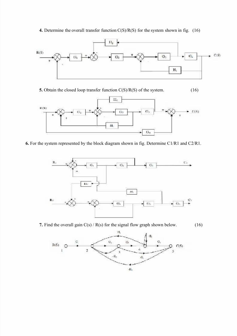
. -etermine the overall transfer function +OSP90OSP for the system shown in fig. O"DP

4. 6btain the closed loop transfer function +OSP90OSP of the system. O"DP

3. 7or the system represented by the block diagram shown in fig. -etermine +"90" and +$90".

J. 7ind the overall gain +OsP 9 0OsP for the signal flow graph shown below. O"DP



". 7ind the overall gain of the system whose signal flow graph is shown in O"DP

11. OiP -erive the transfer function for /rmature controlled -+ motor. OFPOiiP-erive the transfer function for 7ield controlled -+ motor. OFP

1!. OiPExplain -+ servo motor. ODPOiiPExplain the working of /+ servomotor in control systems. O"<P

9. -raw a signal flow graph and evaluate the closed loop transfer function of a system

whose block is shown in fig. O"DP

10. 5rite the differential euations governing the mechanical systems shown below.-raw the force!voltage and force!current electrical analogous circuits and verify bywriting mesh and node euations. O"DP



NI II H I7E RES=ONSE

?O 7ARS

1. ?hat are the 5ai$ ad*a$tage% '# ge$era-iKed err'r c'He##icie$t

iP Steady state is function of time.iiP Steady state can be determined from any type of input

!. ?hat are the e##ect% '# addi$g a Ker' t' a %+%te5

/dding a zero to a system results in pronounced early peak to system response thereby the

peak overshoot increases appreciably.

. StateH7ag$itde criteri'$.

#he magnitude criterion states that ssa will be a point on root locus if for that value of s,

-OsP GOsP 1OsP ". State 8 A$g-e criteri'$.

#he /ngle criterion states that ssa will be a point on root locus for that value of s,

N-OsP NGOsP 1OsP odd multiple of "F<T

4. ?hat i% a d'5i$a$t )'-e

#he dominant pole is a pair of complex conjugate pair which decides the transient response of

the system.

3. Na5e the te%t %ig$a-% %ed i$ c'$tr'- %+%te5

#he commonly used test input signals in control system are impulse step ramp

acceleration and sinusoidal signals.

J. e#i$e BIBO %tai-it+.

/ linear relaxed system is said to have ))6 stability if every bounded input results in a

bounded output.

". ?hat i% the $ece%%ar+ c'$diti'$ #'r %tai-it+

#he necessary condition for stability is that all the coefficients of the characteristic polynomial be positive.

9. ?hat i% the $ece%%ar+ a$d %##icie$t c'$diti'$ #'r %tai-it+

#he necessary and sufficient condition for stability is that all of the elements in the first

column of the routh array should be positive.



10. ?hat i% Dadra$t %+55etr+

#he symmetry of roots with respect to both real and imaginary axis called uadrant

symmetry. 7or a bounded input signal if the output has constant amplitude oscillations then

the system may be stable or unstable under some limited constraints such a system is called

limitedly stable system.

11. ?hat i% %tead+ %tate err'r

#he steady state error is the value of error signal eOtP when t tends to infinity.

1!. ?hat are %tatic err'r c'$%ta$t%

#he =p =v and =a are called static error constants.

1. ?hat i% the di%ad*a$tage i$ )r')'rti'$a- c'$tr'--er

#he disadvantage in proportional controller is that it produces a constant steady state error.1. ?hat i% the e##ect '# = c'$tr'--er '$ %+%te5 )er#'r5a$ce

#he effect of - controller is to increase the damping ratio of the system and so the peak

overshoot is reduced.

14. ?h+ deri*ati*e c'$tr'--er i% $'t %ed i$ c'$tr'- %+%te5

#he derivative controller produces a control action based on rare of change of error signal and

it does not produce corrective measures for any constant error. 1ence derivative controller is

not used in control system13. ?hat i% the e##ect '# =I c'$tr'--er '$ the %+%te5 )er#'r5a$ce

#he ) controller increases the order of the system by one, which results in reducing the

steady state error .ut the system becomes less stable than the original system.

1J. ?hat i% a$ 'rder '# a %+%te5

#he order of a system is the order of the differential euation governing the system. #he order

of the system can be obtained from the transfer function of the given system.

1". e#i$e a5)i$g rati'.

-amping ratio is defined as the ratio of actual damping to critical damping.

19. Li%t the ti5e d'5ai$ %)eci#icati'$%.

#he time domain specifications are i.-elay time ii.0ise time iii.eak time iv.eak

overshoot



!0. e#i$e e-a+ ti5e.

#he time taken for response to reach (<U of final value for the very first time is called delay

time.

!1. e#i$e Ri%e ti5e.

#he time taken for response to rise from <U to "<<U for the very first time is rise time.

!!. e#i$e )ea ti5e.

#he time taken for the response to reach the peak value for the first time is peak time.

!. e#i$e )ea '*er%h''t.

eak overshoot is defined as the ratio of maximum peak value measured from the

:aximum value to final value

!. e#i$e Sett-i$g ti5e.

Settling time is defined as the time taken by the response to reach and stay within specified

error

!4. ?hat i% the $eed #'r a c'$tr'--er

#he controller is provided to modify the error signal for better control /ction

!3. ?hat are the di##ere$t t+)e% '# c'$tr'--er%

roportional controller ) controller

- controller )- controller !J. ?hat i% )r')'rti'$a- c'$tr'--er

)t is device that produces a control signal which is proportional to the input error signal.

!". ?hat i% = c'$tr'--er

- controller is a proportional plus derivative controller which produces an output signal

consisting of two times !one proportional to error signal and other proportional to the

derivative of the signal.

!9. ?hat i% the %ig$i#ica$ce '# i$tegra- c'$tr'--er a$d deri*ati*e c'$tr'--er i$ a =I9

c'$tr'--er

#he proportional controller stabilizes the gain but produces a steady state error. #he integral

control reduces or eliminates the steady state error.



0. ?h+ deri*ati*e c'$tr'--er i% $'t %ed i$ c'$tr'- %+%te5%.

#he derivative controller produces a control action based on the rate of change of error signal

and it does not produce corrective measures for any constant error.

1. e#i$e Stead+ %tate err'r.

#he steady state error is defined as the value of error as time tends to infinity.

!. ?hat i% the drawac '# %tatic c'e##icie$t%

#he main draw back of static coefficient is that it does not show the variation of error with

time and input should be standard input.

. ?hat i% %te) %ig$a-

#he step signal is a signal whose value changes from zero to / at t < and remains constant at

/ for tV<.

. ?hat i% ra5) %ig$a-

#he ramp signal is a signal whose value increases linearly with time from an initial value of

zero at t<.the ramp signal resembles constant velocity.

4. ?hat i% a )ara'-ic %ig$a-

#he parabolic signal is a signal whose value varies as a suare of time from an initial value of

zero at t<.#his parabolic signal represents constant acceleration input to the signal.

3. ?hat are the three c'$%ta$t% a%%'ciated with a %tead+ %tate err'r.ositional error constant, Celocity error constant /cceleration error constant.

J. ?hat are r''t -'ci

#he path taken by the roots of the open loop transfer function when the loop gain is

varied from < to W is called root loci.

%F. ?hat are the 5ai$ %ig$i#ica$ce% '# r''t -'c%.

i. #he main root locus techniue is used for stability analysis.

ii. Qsing root locus techniue the range of values of =, for as table system can be

determined



= A R B

1. (aP -erive the expressions X draw the response of first order system for unit step input. OFP

ObP -raw the response of second order system for critically damped case and when input

is

unit step. OFP

!. -erive the expressions for 0ise time, eak time, eak overshoot, delay timeO"DP

. / positional control system with velocity feedback is shown in fig. 5hat is the response of

the system for unit step input. O"DP

. OiP :easurements conducted on a Servomechanism show the system response to be

cOtP"L<.$ Y!D<t !".$ Y &"< t. when subjected to a unit step. 6btain an expression for closed

loop transfer function. OFP

4. OiP / unity feedback control system has an open loop transfer function GOSP "<9SOSL$P.7indthe rise time, percentage over shoot, peak time and settling time. OFP

OiiP / closed loop servo is represented by the differential euation d$c9dt$ LF dc9dt D' e

5here c is the displacement of the output shaft r is the displacement of the input shaft and e

r!c. -etermine undamped natural freuency, damping ratio and percentage maximum

overshoot for unit step input. OFP

3. 7or a unity feedback control system the open loop transfer function GOSP "<OSL$P9 S$

OSL"P.7ind OaP position, velocity and acceleration error constants.

ObPthe steady state error when the input is 0OSP where 0OSP %9S &$9S$

L"9%S%

O"DP

J. #he open loop transfer function of a servo system with unity feedback system is GOSP "<9

SO<."SL"P. Evaluate the static error constants of the system. 6btain the steady sta0te

e1rror 2of the system when subjected to an input given olynomial rOtP a La t La 9$ t$ O"DP.



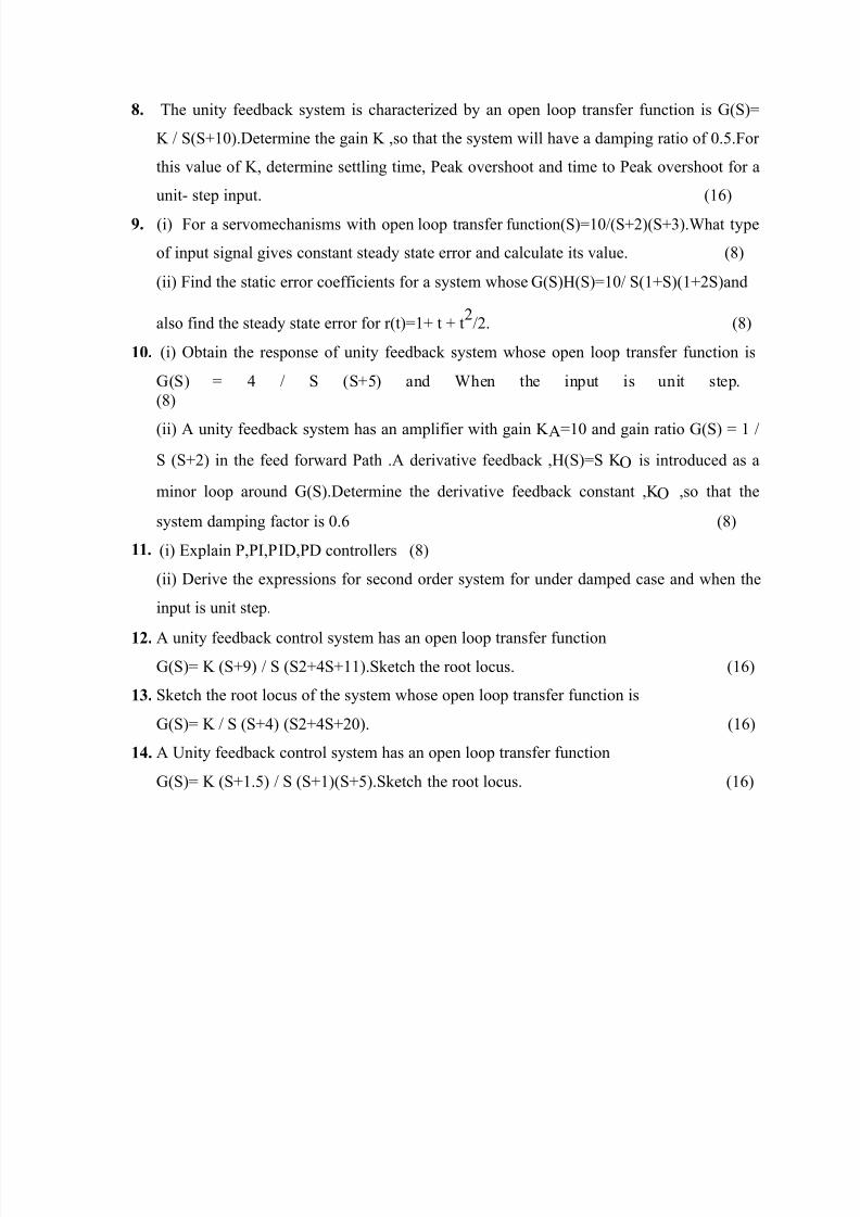
". #he unity feedback system is characterized by an open loop transfer function is GOSP

= 9 SOSL"<P.-etermine the gain = ,so that the system will have a damping ratio of <.(.7or

this value of =, determine settling time, eak overshoot and time to eak overshoot for a

unit! step input. O"DP

9. OiP 7or a servomechanisms with open loop transfer functionOSP"<9OSL$POSL%P.5hat type

of input signal gives constant steady state error and calculate its value. OFP

OiiP 7ind the static error coefficients for a system whose GOSP1OSP"<9 SO"LSPO"L$SPand

also find the steady state error for rOtP"L t L t$9$. OFP

10. OiP 6btain the response of unity feedback system whose open loop transfer function is

GOSP ' 9 S OSL(P and 5hen the input is unit step.OFP

OiiP / unity feedback system has an amplifier with gain = /"< and gain ratio GOSP " 9

S OSL$P in the feed forward ath ./ derivative feedback ,1OSPS = 6 is introduced as a

minor loop around GOSP.-etermine the derivative feedback constant ,= 6 ,so that the

system damping factor is <.D OFP

11. OiP Explain ,),)-,- controllers OFP

OiiP -erive the expressions for second order system for under damped case and when the

input is unit step.

1!. / unity feedback control system has an open loop transfer functionGOSP = OSL?P 9 S OS$L'SL""P.Sketch the root locus. O"DP

1. Sketch the root locus of the system whose open loop transfer function is

GOSP = 9 S OSL'P OS$L'SL$<P. O"DP

1. / Qnity feedback control system has an open loop transfer function

GOSP = OSL".(P 9 S OSL"POSL(P.Sketch the root locus. O"DP



NI III H >R/ENC6 RES=ONSE

?O 7AR0S

1. ?hat i% #reDe$c+ re%)'$%e

/ freuency responses the steady state response of a system when the input to the systemis a sinusoidal signal.

!. ?hat are #reDe$c+ d'5ai$ %)eci#icati'$%

". 0esonant peak '. +ut!off rate

$. 0esonant freuency (. Gain margin

%. andwidth D. hase margin.

. ?hat i% B'de )-'t

#he ode plot is the freuency response plot of the transfer function of a system. )t

consists of two plots!magnitude plot and phase plot. #he magnitude plot is a graph between

magnitude of a system transfer function in db and the freuency Zc . #he phase plot is a graph

between the phase or argument of a system transfer function in degrees and the freuency Z c .

Qsually, both the plots are plotted on a common x!axis in which the freuencies are expressed inlogarithmic scale.

. ?hat i% a))r'i5ate 'de )-'t

)n approximate bode plot, the magnitude plot of first and second order factors are

approximated by two straight lines, which are asymptotes to exact plot. 6ne straight line is at

<db, for the freuency range < to Zc and the other straight line is drawn with a slope of [ $<n

db9dec for the freuency range Zc to Z. 1ere Zc is the corner freuency.

4. ?hat are ad*a$tage% '# B'de )-'t

". #he magnitudes are expressed in db and so a simple procedure is to add magnitude of each

term one by one.



$. #he approximate bode plot can be uickly sketched, and the c\ can be made at corner

freuencies to get the exact plot.

%. #he freuency domain specifications can be easily determined.

'. #he bode plot can be used to analyze both open loop and ck system.

3. ?hat i% the *a-e '# err'r i$ the a))r'i5ate 5ag$itde )-'t '# a #t #act'r at the c'r$er

#reDe$c+

#he error in the approximate magnitude plot of a first order factor at t freuency is[

%mdb, where m is multiplicity factor. ositive error for r factor and negative error for

denominator factor.

J. ?hat i% the *a-e '# err'r i$ the a))r'i5ate 5ag$itde )-'t '# a i #act'r with M- at

the c'r$er #reDe$c+

#he error is [ Ddb, for the uadratic factor with Zl. ositive error for i factorand

negative error for denominator factor.

". e#i$e )ha%e 5argi$.

#he phase margin, is the amount of additional phase lag at the gain cross & over freuency, Zgc

reuired to bring the system to the verge of instability. )t is given by, "F<T L Φ gc, where Φ gc is

the phase of GOjZP at the gain cross over freuency

hase margin, γ = "F<° L Φgc

5her e, Φ gc = /rg J G Ojω PKS

ω

ω gc

9. e#i$e gai$ 5argi$.

#he gain margin, = g is defined as the reciprocal of the magnitude of open loop

transfer function, at phase cross & over freuency, Z pc



"Gain margin, = g

GOP jω ω =ω

pc

5hen expressed in decibels, it is given by, the negative of db magnitude of GO jZ P at phase cross over freuency.

"Gain margin in db $< log GOP j

ω ω =ω

pc

! $< log GOjZP Z Z pc

10.?rite the e)re%%i'$ #'r re%'$a$t )ea a$d re%'$a$t #reDe$c+

#he expression for resonant peak and resonant freuency are

0esonant eak, :r $ζ

"

" − ζ $

G" OP s = pL K

i L = S S

d $0esonant freuency,

K S $ L = S L =

ω r

ω n " − $ζ

d p i

S

11. e#i$e gai$ cr'%% '*er #reDe$c+.

#he gain cross over freuency ω gc is the freuency at which the magnitude of the open

loop transfer function is unity..

1!. e#i$e )ha%e cr'%% '*er #reDe$c+.

#he freuency at which, the phase of open loop transfer functions is called phase cross

over freuency ω pc.

1. e#i$e C'r$er #reDe$c+

#he magnitude plot can be approximated by asymptotic straight lines. #he freuencies

corresponding to the meeting point of asymptotes are called corner freuency. #he slope of the

magnitude plot changes at every corner freuencies.



14. e#i$e 8re%'$a$t =ea

#he maximum value of the magnitude of closed loop transfer function is called resonant

peak.

14. e#i$e 8Re%'$a$t #reDe$c+.

#he freuency at which resonant peak occurs is called resonant freuency.

13. ?hat i% a$dwidth

#he bandwidth is the range of freuencies for which the system gain )s more than %

db.#he bandwidth is a measure of the ability of a feedback system to reproduce the input

signal ,noise rejection characteristics and rise time.

1J. e#i$e CtH'## rate

#he slope of the log!magnitude curve near the cut!off is called cut!off rate. #he cut!off

rate indicates the ability to distinguish the signal from noise.

1". ?hat are 7 a$d N circ-e%

#he magnitude, : of closed loop transfer function with unity feedback will be in the

form of circle in complex plane for each constant value of :. #he family of these circles arecalled : circles.

8et 2 tan Z where a is the phase of closed loop transfer function with unity feedback.

7or each constant value of 2, a circle can be drawn in the complex plane. #he family of these

circles are called 2 circles.

19.?hat are tw' c'$t'r% '# Nich'-% chart

2ichols chart of : and 2 contours, superimposed on ordinary graph. #he : contours arethe magnitude of closed loop system in decibels and the 2 contours are the phase angle locus of

closed loop system.



!0. ?hat i% Nich'-% chart

#he 2ichols chart consists of : and 2 contours superimposed on ordinary graph. /long

each : contour the magnitude of closed loop system, : will be a constant. /long each 2

contour, the phase N of closed loop system will be constant. #he ordinary graph consists ofmagnitude in db, marked on the y!axis and the phase in degrees marked on x!axis. #he 2ichols

chart is used to find the closed loop freuency response from the open loop freuency response

!1. <'w i% the Re%'$a$t =ea(7r, re%'$a$t #reDe$c+(?r , a$d a$d width deter5i$ed

#r'5 Nich'-% chart

iP #he resonant peak is given by the value of µ.contour which is tangent to GOjω P locus.

iiP #he resonant freuency is given by the freuency of GOjω P at the tangency point.

iiiP #he bandwidth is given by freuency corresponding to the intersection point of GOjω P

and &%d :!contour.

!!. ?hat are the ad*a$tage% '# Nich'-% chart

". )t is used to find closed loop freuency response from open loop freuency response.

$. #he freuency domain specifications can be determined from 2ichols chart.

%. #he gain of the system can be adjusted to satisfy the given specification.

!. ?rite a %h'rt $'te '$ the c'rre-ati'$ etwee$ the ti5e a$d #reDe$c+ re%)'$%e

#here exist a correlation between time and freuency response of first or second order

systems. #he freuency domain specification can be expressed in terms of the time domain

parameters N, and N . 7or a peak overshoot in time domain there is a corresponding resonant peak

in freuency domain. 7or higher order systems there is no explicit correlation between time and

freuency response. ut if there is a pair of dominant complex conjugate poles, then the system

can be approximated to second order system and the correlation between time and freuency

response can be estimated.

!. <'w c-'%ed -'') #reDe$c+ re%)'$%e i% deter5i$ed #r'5 ')e$ -'') #reDe$c+ re%)'$%e

%i$g 7 a$d Ncirc-e%

#he GOj ZP locus or the polar plot of open loop system is sketched on the standard : and

2 circles chart. #he meeting point of : circle with GOj ZP locus gives the magnitude of closed



loop system, Othe freuency being same as that of open loop systemP. #he meeting point of GOj

ZP locus with 2!circle gives the value of phase of closed loop system, Othe freuency being same

as that of open loop systemP.

!4. ?hat i% )'-ar )-'t

#he polar plot of a sinusoidal transfer function GOj ZP is a plot of the magnitude of GOj ZP

versus the phase angle9argument of GOj ZP on polar or rectangular coordinates as N is varied

from zero to infinity.

!3. ?hat i% 5i$i55 )ha%e %+%te5

#he minimum phase systems are systems with minimum phase transfer functions. )n

minimum phase transfer functions, all poles and zeros will lie on the left half of s!plane.

!J. ?hat i% A--H=a%% %+%te5%

#he all pass systems are systems with all pass transfer functions. )n all pass transfer

functions, the magnitude is unity at all freuencies and the transfer function will have anti!

symmetric pole zero pattern Oi.e., for every pole in the left half s!plane, there is a zero in the

mirror image position with respect to imaginary axisP.

$F. ?hat are the ad*a$tage% i$ #reDe$c+ d'5ai$ de%ig$

#he advantages in freuency domain design ar e

". #he effect of disturbances, sensor noise and plant uncertainties are easy to visualizeand accesses in freuency domain.

$. #he experimental information can be used for design purposes.

$?. ?hat i% a Nich'-% )-'t

#he 2ichols plot is a freuency response plot of the open loop transfer function of a

system. )t is a graph between magnitude of GOj ZP in db and the phase of GOj ZP in degree,

plotted on a ordinary graph sheet.

%<. <'w the c-'%ed -'') #reDe$c+ re%)'$%e i% deter5i$ed #r'5 the ')e$ -'') #reDe$c+

re%)'$%e %i$g Nich'-% chart

#he GOj ZP locus or the 2ichols plot is sketched on the standard 2ichols chart. #he

meeting point of : contour with GOj ZP locus gives the magnitude of closed loop system and the

meeting point with 2 circle gives the argument9phase of the closed loop system.



=A R B

1. lot the ode diagram for the following transfer function and obtain the gain and phase cross

over freuencies. GOSP "<9 SO"L<.'SP O"L<."SP O"DP

!. #he open loop transfer function of a unity feed back system is GOSP "9 SO"LSP O"L$SP.

Sketch the olar plot and determine the Gain margin and hase margin. O"DP

. Sketch the ode plot and hence find Gain cross over freuency ,hase cross over

freuency, Gain margin and hase margin.

GOSP <.B(O"L<.$SP9 SO"L<.(SP O"L<."SP O"DP

. Sketch the ode plot and hence find Gain cross over freuency, hase cross over


GOSP "<OSL%P9 SOSL$P OS$L'SL"<<P O"DP4. Sketch the polar plot for the following transfer function .and find Gain cross over

freuency ,hase cross over freuency, Gain margin and hase margin.

GOSP "<OSL$POSL'P9 S OS$ !%SL"<P O"DP

3. +onstruct the polar plot for the function G1OSP $OSL"P9 S$. find Gain cross over

freuency ,hase cross over freuency, Gain margin and hase margin. O"DP

J. lot the ode diagram for the following transfer function and obtain the gain and phase

cross over freuencies GOSP =S$ 9 O"L<.$SP O"L<.<$SP.-etermine the value of = for again cross over freuency of $< rad9sec. O"DP

". Sketch the polar plot for the following transfer function .and find Gain cross over

freuency, hase cross over freuency, Gain margin and hase margin.

GOSP '<<9 S OSL$POSL"<P O"DP

9. / unity feed back system has open loop transfer function GOSP $<9 S OSL$POSL(P.Qsing

2ichol*s chart. -etermine the closed loop freuency response and estimate all the freuency

domain specifications. O"DP

10. Sketch the ode plot and hence find Gain cross over freuency, hase cross over


GOSP "<O"L<."SP9 SO"L<.<"SP O"LSP. O"DP



NI I; H SABILI6 AN CO7=ENSAOR

ESIGN ?O 7ARS

1. ?hat are the e##ect% '# addi$g a Ker' t' a %+%te5

/dding a zero to a system increases peak overshoot appreciably.

!. e#i$e Re-ati*e %tai-it+

0elative stability is the degree of closeness of the system, it is an indication of

strength or degree of stability.

. ?hat i% )ha%e 5argi$

#he phase margin is the amount of phase lag at the gain cross over freuency reuired

to bring system to the verge of instability.

. e#i$e Gai$ cr'%% '*er

#he gain cross over freuency is the freuency at which the magnitude of the open

loop transfer function is unity.

4. ?hat i% B'de )-'t

#he ode plot is the freuency response plot of the transfer function of a system. /

ode plot consists of two graphs. 6ne is the plot of magnitude of sinusoidal transfer

function versus log Z.#he other is a plot of the phase angle of a sinusoidal function versus

logZ.

3. ?hat are the 5ai$ ad*a$tage% '# B'de )-'t

#he main advantages are\

iP :ultiplication of magnitude can be in to addition.

iiP / simple method for sketching an approximate log curve is available.

iiiP )t is based on asymptotic approximation. Such approximation is sufficient if

rough information on the freuency response characteristic is needed.

ivP #he phase angle curves can be easily drawn if a template for the phase angle

curves of "L j Z is available.

J. e#i$e C'r$er #reDe$c+

#he freuency at which the two asymptotic meet in a magnitude plot is called corner

freuency.



". ?hat i% a$dwidth

#he bandwidth is the range of freuencies for which the system gain is more than %

db. #he bandwidth is a measure of the ability of a feedback system to reproduce the input

signal, noise rejection characteristics and rise time.

9. e#i$e CtH'## rate

#he slope of the log!magnitude curve near the cut!off is called cut!off rate. #he cut!

off rate indicates the ability to distinguish the signal from noise.

"<. ?hat are the ti5e d'5ai$ %)eci#icati'$% $eeded t' de%ig$ a c'$tr'- %+%te5

". 0ise time, tr $. eak overshoot , :p %. Setting time, ts '.-amping ratio

(. 2atural freuency of oscillation, Nn

11. ?rite the $ece%%ar+ #reDe$c+ d'5ai$ %)eci#icati'$ #'r de%ig$ '# a c'$tr'- %+%te5.

". hase margin $. Gain margin %. 0esonant peak '. andwidth

1!. ?hat i% c'5)e$%ati'$

#he compensation is the design procedure in which the system behavior is altered to

meet the desired specifications by introducing additional device called compensator.

"%. ?hat i% a c'5)e$%at'r

/ device inserted in to the system for the purpose of satisfying the specifications is

called compensator.

1. ?hat are the di##ere$t t+)e% '# c'5)e$%at'r

". 8ag compensator

$. 8ead compensator

%. 8ag & lead compensator.

"(. ?he$ -ag : -ead : -ag 8 -ead c'5)e$%at'r i% e5)-'+ed

#he lag compensator is employed for a stable system for improvement in steady state

performance.

#he lead compensation is employed for stable 9 unstable system for improvement in

transient & state performance.

#he lag & lead compensation is employed for stable 9 unstable system for

improvement in both steady state and transient state performance.



13. e#i$e =ha%e -ag a$d )ha%e -ead

/ negative phase angle is called phase lag.

/ positive phase angle is called phase lead.

1J. ?hat are the tw' t+)e% '# c'5)e$%ati'$ %che5e%

i. +ascade or series compensation

ii. 7eedback compensation or parallel compensation

1". ?hat i% %erie% c'5)e$%ati'$

#he series compensation is a design procedure in which a compensator is introduced in

series with plant to alter the system behaviour and to provide satisfactory performance Oi.e., to

meet the desired specificationsP.

Gc OsP #ransfer function of series compensator

G OsP 6pen loop transfer function of the plant

1 OsP 7eedback path transfer function.

19. ?hat i% #eedac c'5)e$%ati'$

#he feedback compensation is a design procedure in which a compensator is introduced

in the feedback path so as to meet the desired specifications. )t is also called parallel

compensation.

Gc OsP #ransfer function of series compensator,G" OsP G$ OsP 6pen loop transfer function of

the plant 1 OsP 7eedback path transfer function.

!0. ?hat are the #act'r% t' e c'$%idered #'r ch''%i$g %erie% 'r %h$t:#eedac

c'5)e$%ati'$

#he choice between series, shunt or feedback compensation depends on the following\

2ature of signals in the systems. ower levels at various points. +omponents available.

-esigner*s experience. Economic considerations.

!1. ?h+ c'5)e$%ati'$ i% $ece%%ar+ i$ #eedac c'$tr'- %+%te5

)n feedback control systems compensation is reuired in the following situations. 5hen

the system is absolutely unstable, then compensation is reuired to stabilize the system and also

to meet the desired performance. 5hen the system is stable, compensation is provided to obtain

the desired performance.



!!. i%c%% the e##ect '# addi$g a )'-e t' ')e$ -'') tra$%#er #$cti'$ '# a %+%te5.

#he addition of a pole to open loop transfer function of a system will reduce the steady

state error. #he closer the pole to origin lesser will be the steady!state error. #hus the steady!

state performance of the system is improved. /lso the addition of pole will increase the order of

the system, which in turn makes the system less stable than the original system.

!. i%c%% the e##ect '# addi$g a Ker' t' ')e$ -'') tra$%#er #$cti'$ '# a %+%te5.

#he addition of a zero to open loop transfer function of a system will improve the

transient response. #he addition of zero reduces the rise time. )f the zero is introduced close to

origin then the peak overshoot will be larger. )f the zero is introduced far

/way from the origin in the left half of s!plane then the effect of zero on the transient response

will be negligible.

!. ?hat are the ad*a$tage% a$d di%ad*a$tage% i$ #reDe$c+ d'5ai$ de%ig$

#he effect of disturbances, sensor noise and plant uncertainties are easy to visualize and

asses in freuency domain. #he experimental information can be used for design purposes.

#he disadvantages of freuency response design are that it gives the information on

closed loop system*s transient response indirectly.

!4. ?hat are the %e% '# -ead c'5)e$%at'r

• speeds up the transient response

• increases the margin of stability of a system

• increases the system error constant to a limited extent.

!3. ?hat i% -agHc'5)e$%ati'$

#he lag compensation is a design procedure in which a lag compensator is introduced in

the system so as to meet the desired specifications.

$B. ?hat i% a -ag c'5)e$%at'r Gi*e a$ ea5)-e.

/ compensator having the characteristics of lag network is called lag compensator. )f a

sinusoidal signal is applied to a lag compensator, then in steady state the output will have a phase

lag and lead with respect to input.



!". ?hat are the characteri%tic% '# -ag c'5)e$%ati'$ ?he$ -ag c'5)e$%ati'$ i%

e5)-'+ed

#he lag compensation improves the steady state performance, reduces the bandwidth and

increases the rise time. #he increase in rise time results in slower transient response. )f the zero

in the system does not cancel the pole introduced by the compensator, then lag compensator

increases the order of the system by one.

5hen the given system is stable and does not satisfy the steady!state performance

specifications then lag compensation can be employed so that the system is redesigned to satisfy

the steady!state reuirements.

$?. ?hat i% -ead c'5)e$%ati'$

#he lead compensation is a design procedure in which a lead compensator is introduced

in the system so as to meet the desired specifications.

0. ?hat are the characteri%tic% '# -ead c'5)e$%ati'$ ?he$ -ead c'5)e$%ati'$ i%

e5)-'+ed

#he lead compensation increases the bandwidth and improves the speed of response. )t

also reduces the peak overshoot. )f the pole introduced by the compensator is not cancelled by

the zero in the system, then lead compensation increases the order of the system by one. 5hen

the given system is stable9 unstable and reuires improvement in transient state response then

lead compensation is employed.



= A R B

". OiP Qsing 0outh criterion determine the stability of the system whose characteristics

euation is S'LFS%L"FS$L"DSL( <. OFP

OiiP.7OSP SD LS(!$S'!%S%!BS$!'S!' <.7ind the number of roots falling in the 01S

plane and 81S plane. OFP

$. / unity feedback control system has an open loop transfer function

GOSP = 9 S OS$L'SL"%P.Sketch the root locus. O"DP

%. -raw the 2yuist plot for the system whose open loop transfer function is

GOSP= 9 S OSL$POSL"<P. -etermine the range of k for which closed loop system is

stable. O"DP

'. Sketch the 2yuist lot for a system with the open loop transfer functionGOSP 1OSP = O"L<.(SPO"LSP 9 O"L"<SPOS!"P. -etermine the range of k for which closed

loop system is stable. O"DP

(. OiP -etermine the range of = for stability of unity feedback system whose open loop

transfer function is GOsP = 9 s OsL"POsL$P OFP

OiiP #he open loop transfer function of a unity feed back system is given by

GOsP = OsL"P 9 s%Las$L$sL". -etermine the value of = and a so that the system

oscillates at a freuency of $ rad9sec. OFP

D. (iP +onstruct 0outh array and determine the stability of the system represented by the

characteristics euation S(LS'L$S%L$S$L%SL(<.+omment on the location of the roots

of characteristic euation. OFP

OiiP +onstruct 0outh array and determine the stability of the system represented by the

characteristics euation SBL?SDL$'S'L$'S%L$'S$L$%SL"(<comment on the location

of the roots of characteristic euation.

B. 5hat is compensation] 5hy it is need for control system] Explain the types of

compensation] 5hat is an importance of compensation] O"DP

F. 0ealise the basic compensators using electrical network and obtain the transfer

function. O"DP

?. -esign suitable lead compensators for a system unity feedback and having open loop

transfer function GOSP =9 SOSL"P to meet the specifications.OiP #he phase margin of the



system ^ '(_, OiiP Steady state error for a unit ramp input `"9"(, OiiiP #he gain cross over

freuency of the system must be less than B.( rad9sec. O"DP

"<. / unity feed back system has an open loop transfer function GOSP =9 SOSL"P O<.$SL"P.

-esign a suitable phase lag compensators to achieve following specifications =v F

and hase margin '< deg with usual notation. O"DP

"". Explain the procedure for lead compensation and lag compensation O"DP

"$. Explain the design procedure for lag! lead compensation O"DP

"%. +onsider a type " unity feed back system with an 68#7 GOSP =9S OSL"P OSL'P. #he

system is to be compensated to meet the following specifications =v V (sec and : V '%

deg. -esign suitable lag compensators.

"'. -esign a lead compensator for a unity feedback system with open loop transfer function

GOSP =9 SOSL"P OSL(P to satisfy the following specifications OiP =v V (< OiiP hase:argin is V $< . O"DP

"(. -esign a lead compensator for GOSP = 9 S$ O<.$SL"P to meet the following

Specifications OiP/cceleration ka"<> OiiP .:%(. O"DP

"D. -esign a 8ag compensator for the unity feedback system whose closed loop transfer

function +OsP 9 0OsP = 9 Os OsL'P OsLF<P L =P is to meet the following specifications

.: ^%% _. /nd =v ^%<. O"DP

"B. / unity feedback system has an 68#7 GOsP = 9 sOsL$POsLD<P. -esign a 8ead!8agcompensator is to meet the following specifications.

OiP .: is atleast '<_ , OiiP Steady state error for ramp input ` <.<' rad. O"D



1. e#i$e %tate *aria-e.

NI ; H STATE VARIABLE ANALYSIS

?O 7AR0S

#he state of a dynamical system is a minimal set of variablesOknown as state variablesP such

that the knowledge of these variables at t!t< together with the knowledge of the inputs for t V t< ,

completely determines the behavior of the system for t V t<

!. ?rite the ge$era- #'r5 '# %tate *aria-e 5atri.

#he most general state!space representation of a linear system with m inputs, p outputs and n

state variables is written in the following form\

/ L Q

R + L -Q

5here state vector of order n ".

Q input vector of order n ".

/System matrix of order n n.

)nput matrix of order n m

+ output matrix of order p n

- transmission matrix of order p m

. ?rite the re-ati'$%hi) etwee$ KHd'5ai$ a$d %Hd'5ai$.

/ll the poles lying in the left half of the S!plane, the system is stable in S!domain.+orresponding in !domain all poles lie within the unit circle.

. ?hat are the 5eth'd% a*ai-a-e #'r the %tai-it+ a$a-+%i% '# %a5)-ed data c'$tr'- %+%te5

#he following three methods are available for the stability analysis of sampled data control

system

". uri*s stability test.

$. ilinear transformation.

%. 0oot locus techniue.4. ?hat i% the $ece%%ar+ c'$diti'$ t' e %ati%#ied #'r de%ig$ %i$g %tate #eedac

#he state feedback design reuires arbitrary pole placements to achieve the desire performance.

#he necessary and sufficient condition to be satisfied for arbitrary pole placement is that the system is

completely state controllable.



3. ?hat i% c'$tr'--ai-it+

/ system is said to be completely state controllable if it is possible to transfer the system state

from any initial state Ot<P at any other desired state OtP, in specified finite time by a control vector

QOtP.

J. ?hat i% '%er*ai-it+

/ system is said to be completely observable if every state OtP can be completely identified by

measurements of the output ROtP over a finite time interval.

". ?rite the )r')ertie% '# %tate tra$%iti'$ 5atri.

#he following are the properties of state transition matrix

". O<P e/x< ) Ounit matrixP.

$. OtP e/t Oe!/tP!" JO!tPK!".

%. Ot"Lt$P e/Ot"Lt$P Ot"P Ot$P Ot$P Ot"P.

9. e#i$e %a5)-i$g the're5.

Sampling theorem states that a band limited continuous time signal with highest freuency f m,

hertz can be uniuely recovered from its samples provided that the sampling rate 7s is greater than or

eual to $f m samples per second.

10. ?hat i% %a5)-ed data c'$tr'- %+%te5

5hen the signal or information at any or some points in a system is in the form of discrete

pulses, then the system is called discrete data system or sampled data system.11. ?hat i% N+Di%t rate

#he Sampling freuency eual to twice the highest freuency of the signal is called as 2yuist

rate. f s$f m

1!. ?hat i% %i5i-arit+ tra$%#'r5ati'$

#he process of transforming a suare matrix A to another similar matrix B by a transformation

=H1

A= M B is called similarity transformation. #he matrix is called transformation matrix.

1. ?hat i% 5ea$t + diag'$a-iKati'$

#he process of converting the system matrix A into a diagonal matrix by a similarity

transformation using the modal matrix 7 is called diagonalization

1. ?hat i% 5'da- 5atri

#he modal matrix is a matrix used to diagonalize the system matrix. )t is also called

diagonalization matrix.



)f / system matrix.

: :odal matrix

/nd :!"inverse of modal matrix.

#hen :!"/: will be a diagonalized system matrix.

14. <'w the 5'da- 5atri i% deter5i$ed

#he modal matrix : can be formed from eigenvectors. 8et m", m$, m% M. mn be the

eigenvectors of the nth order system. 2ow the modal matrix : is obtained by arranging all the

eigenvectors column wise as shown below.

:odal matrix , : Jm", m$, m% M. mnK.

13. ?hat i% the $eed #'r c'$tr'--ai-it+ te%t

#he controllability test is necessary to find the usefulness of a state variable. )f the state

variables are controllable then by controlling Oi.e. varyingP the state variables the desired outputs of thesystem are achieved.

1J. ?hat i% the $eed #'r '%er*ai-it+ te%t

#he observability test is necessary to find whether the state variables are measurable or not. )f

the state variables are measurable then the state of the system can be determined by practical

measurements of the state variables.

1". State the c'$diti'$ #'r c'$tr'--ai-it+ + Gi-ert’% 5eth'd.

Ca%e (i whe$ the eige$ *a-e% are di%ti$ct

+onsider the canonical form of state model shown below which is obtained by using the

transformation :.

L Q

R L -Q

5here, :!"/:> +: , :!" and : :odal matrix.

)n this case the necessary and sufficient condition for complete controllability is that, the matrix

must have no row with all zeros. )f any row of the matrix is zero then the corresponding state

variable is uncontrollable.

Ca%e(ii whe$ eige$ *a-e% ha*e 5-ti)-icit+

)n this case the state modal can be converted to ordan canonical form shown below

L Q



R L -Q 5here, :!"/:

)n this case the system is completely controllable, if the elements of any row of that correspond to

the last row of each ordan block are not all zero.

19. State the c'$diti'$ #'r '%er*ai-it+ + Gi-ert’% 5eth'd.+onsider the transformed canonical or ordan canonical form of the state model shown below

which is obtained by using the transformation, :

L Q

R L -Q O6rP

L Q

R L -Q where +: and :modal matrix.

#he necessary and sufficient condition for complete observability is that none of the columns of the

matrix be zero. )f any of the column is of has all zeros then the corresponding state variable is not

observable.

!0. State the da-it+ etwee$ c'$tr'--ai-it+ a$d '%er*ai-it+.

#he concept of controllability and observability are dual concepts and it is proposed by kalman as

principle of duality.#he principle of duality states that a system is completely state controllable if and

only if its dual system is completely state controllable if and only if its dual system is completely

observable or viceversa.!1. ?hat i% the $eed #'r %tate '%er*er

)n certain systems the state variables may not be available for measurement and feedback. )n

such situations we need to estimate the unmeasurable state variables from the knowledge of input and

output. 1ence a state observer is employed which estimates the state variables from the input and

output of the system. #he estimated state variable can be used for feedback to design the system by

pole placement.

!!. <'w wi-- +' #i$d the tra$%#'r5ati'$ 5atri, =' t' tra$%#'r5 the %tate 5'de- t' '%er*a-e

)ha%e *aria-e #'r5

• +ompute the composite matrix for observability,<

• -etermine the characteristic euation of the system ) !/ <.

• Qsing the coefficients a",a$,M.an!" of characteristic euation form a matrix, 5.

• 2ow the transformation matrix, < is given by <5 <#.



!. ?rite the '%er*a-e )ha%e *aria-e #'r5 '# %tate 5'de-.

#he observable phase variable form of state model is given by the following euations

/< L <u.

R +< L -u

5here, /< , < and +< J < < M.. < " K

!. ?hat i% the )'-e )-ace5e$t + %tate #eedac

#he pole placement by state feedback is a control system design techniue, in which the state

variables are used for feedback to achieve the desired closed loop poles.

!4. <'w c'$tr'- %+%te5 de%ig$ i% carried i$ %tate %)ace

)n state space design of control system, any inner parameter or variable of a system are used for feedback to achieve the desired performance of the system. #he performance of the system is related to

the location of closed loop poles. 1ence in state space design the closed loop poles are placed at the

desired location by means of state feedback through an appropriate state feedback gain matrix, =.

!3. ?hat are the characteri%tic% 'r )r')ert+ that are i$*aria$t $der a %i5i-arit+ tra$%#'r5ati'$

#he determinant, characteristic euation, eigen values and trace of a matrix are invariant under a

similarity transformation.

!J. ?hat are the ad*a$tage% '# c'$tr'- %+%te5 i$ %tate %)ace

". /ny inner parameters or variables of a system can be defined as state variables and can be used

for feedback.

$. #he closed loop poles may be placed at any desired locations by means of state feedback

through an appropriate state feedback gain matrix, =.

!". ?hat i% the $ece%%ar+ c'$diti'$ t' e %ati%#ied #'r de%ig$ '# %tate '%er*er

#he state observer can be designed only if the system is completely state observable.

!9. ?hat i% c'$tr'- Law

)n control system design using state variable feedback , the euation u r ! = is called controllaw. 5here, u )nput to the plant \ r )nput to the system with state feedback

State vector \ = State feedback gain matrix.

0. ?hat i% ca$'$ica- #'r5 '# %tate 5'de-

)f the system matrix, / is in the form of diagonal matrix then the state model is called canonical

form.



=AR,HB

". 7or

+ompute the state transition matrix e/t using +ayley & 1amilton #heorem. O"DP

$. 7or the system shown in the figure below choose C"OtP and C$OtP as state variables and write down the

state euations satisfied by them. ring these euations in the vector matrix form.

0": ohm, + "7 O"DP

%. / feedback system has a closed loop transfer function,

.

+onstruct three different state models for this system and give block diagram representation for each

state model. O"DP

'. / feedback system is characterized by the closed loop transfer function

.

-raw a suitable signal flow graph and therefrom construct a state model of the system. O"DP

(. Given . +ompute e/t. O"DP



D. 7or a system represented by the state euation. . #he response of .

5hen O<P and . 5hen O<P . -etermine the system matrix / and the

state transition matrix. O"DP

B. / 8#) system is described by the following state model. u.

#ransform this state model into canonical state model and therefrom obtain the explicit solution for the

state vector and output when the control force u is a unit step function and initial state vector is

. O"DP

F. 5rite the state euations of the system shown in figure below in which ", $, and % constitute the

state vector. -etermine whether the system is completely controllable and observable. O"DP

?. +onsider a linear system described by the transfer unction ROsP 9 QOsP "< 9 sOsL"POsL$P.-esign a

feedback controller with a state feedback so thst the closed loop poles are !$, !"L j". O"DP

"<. #he system matrix / of a discrete time system is given by / J< "K

J!$ !%K.

+ompute the state transition matrix /= QS)2G +ayley & 1amilton theorem. O"DP

IC6501 - CS 2 MARKS WITH ANSWERS.doc

Documents

Transcript of IC6501 - CS 2 MARKS WITH ANSWERS.doc