
IC6501-CONTROL SYSTEMS - | Anna University Notes...
49
IC6501-CONTROL SYSTEMS Fatima Michael College of Engineering & Technology Fatima Michael College of Engineering & Technology www.studentsfocus.com
Transcript of IC6501-CONTROL SYSTEMS - | Anna University Notes...

IC6501-CONTROL SYSTEMS
Fatima Michael College of Engineering & Technology
Fatima Michael College of Engineering & Technology
www.studentsfocus.com
Control System
x Control System means any quantity of interest in a machine or mechanism is maintained or altered in accordance with desired manner
x A system which controls the output quantity is called a control system
Definitions:
x Controlled Variable: It is the quantity or condition that is measured & controlled
x Controller: Controller means measuring the value of the controlled variable of the system & applying the manipulated variable to the system to correct or to limit the deviation of the measured value to the desired value.
x Plant: A plant is a piece of equipment, which is a set of machine parts functioning together. The purpose of which is to perform a particular operation. Example: Furnace, Space craft etc.,
x System: A system is a combination of components that works together & performs certain objective.
x Disturbance: A disturbance is a signal that tends to affect the value of the output of a system. If disturbances created inside the system, it is called internal While an external disturbance is generated outside the system.
x Feedback Control: It is an operation that, in the presence of disturbance tends to reduce the difference between the output of a system & some reference input.
x Servo Mechanism: servo mechanism is a feedback controlled system in which the output is some mechanical position, velocity or acceleration.
x Open loop System: In an Open loop System, the control action is independent of the desired output. OR When the output quantity of the control system is not fed back to the input quantity, the control system is called an Open loop System.
x Closed loop System: In the Closed loop Control System the control action is dependent on the desired output, where the output quantity is considerably controlled by sending a command signal to input quantity
3
Basic elements in control systems – Open and closed loop systems – Electrical analogy of Mechanical and thermal systems – Transfer function – Synchros – AC and DC servomotors –Block diagram reduction techniques – Signal flow graphs.
UNIT I SYSTEMS AND THEIR REPRESENTATION
Fatima Michael College of Engineering & Technology
Fatima Michael College of Engineering & Technology
www.studentsfocus.com
4
Classification of Control Systems The Control System can be classified mainly depending upon,
(a) ) Method of analysis & design, as Linear & Non- Linear Systems.
(b)The type of the signal, as Time Varying, Time Invariant, Continuous data, Discrete data systems etc.
(c) The type of system components, as Electro Mechanical, Hydraulic, Thermal, Pneumatic Control systems etc.
(d)The main purpose, as Position control & Velocity control Systems. Linear & Non -Linear Systems:
In a linear system, the principle of superposition can be applied. In non- linear system, principle & homogeneity.
Time Varying & Time Invariant Systems:
x While operating a control system, if the parameters are unaffected by the time, then the system is called Time Invariant Control System.
x Most physical systems have parameters changing with time. If this variation is measurable during the system operation then the system is called Time Varying System.
x If there is no non-linearity in the time varying system, then the system may be called as Linear Time varying System.
Discrete Data Systems:
x If the signal is not continuously varying with time but it is in the form of pulses. Thenthe control system is called Discrete Data Control System.
x If the signal is in the form of pulse data, then the system is called Sampled Data Control System.
x Here the information supplied intermittently at specific instants of time. This has the advantage of Time sharing system.
x On the other hand, if the signal is in the form of digital code, the system is called Digital Coded System.
x Here use of Digital computers, µp, µc is made use of such systems are analyzed by the Z- transform theory.
Continuous Data Systems:
If the signal obtained at various parts of the system are varying continuously with time,then the system is called Continuous Data Control Systems.
Fatima Michael College of Engineering & Technology
Fatima Michael College of Engineering & Technology
www.studentsfocus.com
5
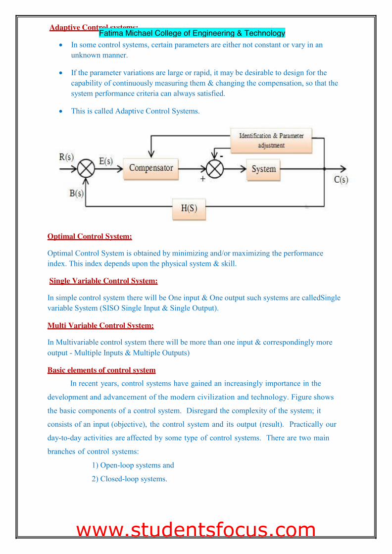
Adaptive Control systems:
x In some control systems, certain parameters are either not constant or vary in an unknown manner.
x If the parameter variations are large or rapid, it may be desirable to design for the capability of continuously measuring them & changing the compensation, so that the system performance criteria can always satisfied.
x This is called Adaptive Control Systems. Optimal Control System:
Optimal Control System is obtained by minimizing and/or maximizing the performance index. This index depends upon the physical system & skill.
Single Variable Control System:
In simple control system there will be One input & One output such systems are calledSingle variable System (SISO Single Input & Single Output).
Multi Variable Control System:
In Multivariable control system there will be more than one input & correspondingly more output - Multiple Inputs & Multiple Outputs)
Basic elements of control system
In recent years, control systems have gained an increasingly importance in the
development and advancement of the modern civilization and technology. Figure shows
the basic components of a control system. Disregard the complexity of the system; it
consists of an input (objective), the control system and its output (result). Practically our
day-to-day activities are affected by some type of control systems. There are two main
branches of control systems:
1) Open-loop systems and
2) Closed-loop systems.
Fatima Michael College of Engineering & Technology
Fatima Michael College of Engineering & Technology
www.studentsfocus.com
6
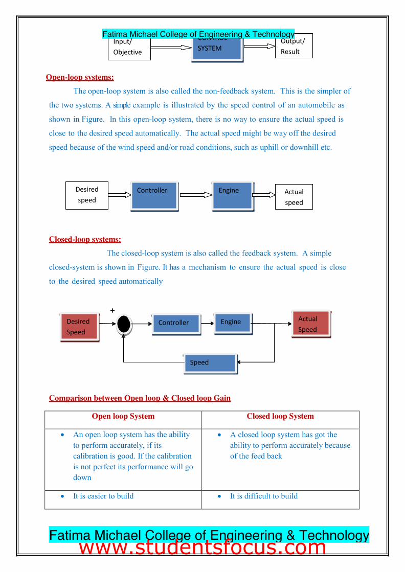
Open-loop systems: The open-loop system is also called the non-feedback system. This is the simpler of
the two systems. A simple example is illustrated by the speed control of an automobile as
shown in Figure. In this open-loop system, there is no way to ensure the actual speed is
close to the desired speed automatically. The actual speed might be way off the desired
speed because of the wind speed and/or road conditions, such as uphill or downhill etc.
Closed-loop systems: The closed-loop system is also called the feedback system. A simple
closed-system is shown in Figure. It has a mechanism to ensure the actual speed is close
to the desired speed automatically
Comparison between Open loop & Closed loop Gain
Open loop System Closed loop System
x An open loop system has the ability to perform accurately, if its calibration is good. If the calibration is not perfect its performance will go down
x A closed loop system has got the ability to perform accurately because of the feed back
x It is easier to build x It is difficult to build
Actual Speed
Desired Speed
Engine Controller
Speed
+
_
Desired speed
Controller Engine Actual speed
CONTROL SYSTEM
Input/ Objective
Output/ Result
Fatima Michael College of Engineering & Technology
Fatima Michael College of Engineering & Technology
www.studentsfocus.com
7
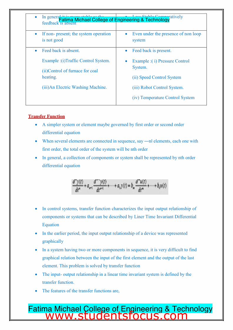
x In general it is more stable as the feedback is absent
x Less Stable Comparatively
x If non- present; the system operation is not good
x Even under the presence of non loop system
x Feed back is absent.
Example :(i)Traffic Control System.
(ii)Control of furnace for coal heating.
(iii)An Electric Washing Machine.
x Feed back is present.
x Example :( i) Pressure Control System.
(ii) Speed Control System
(iii) Robot Control System.
(iv) Temperature Control System
Transfer Function
x A simpler system or element maybe governed by first order or second order
differential equation
x When several elements are connected in sequence, say ―n‖ elements, each one with
first order, the total order of the system will be nth order
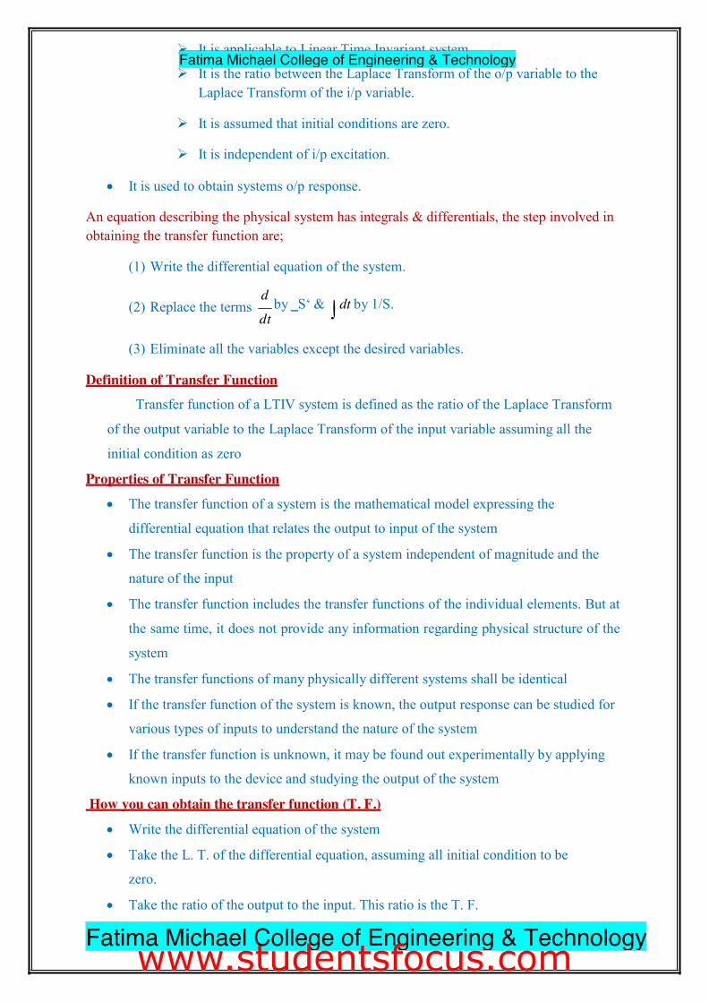
x In general, a collection of components or system shall be represented by nth order
differential equation
x In control systems, transfer function characterizes the input output relationship of
components or systems that can be described by Liner Time Invariant Differential
Equation
x In the earlier period, the input output relationship of a device was represented
graphically
x In a system having two or more components in sequence, it is very difficult to find
graphical relation between the input of the first element and the output of the last
element. This problem is solved by transfer function
x The input- output relationship in a linear time invariant system is defined by the
transfer function.
x The features of the transfer functions are,
Fatima Michael College of Engineering & Technology
Fatima Michael College of Engineering & Technology
www.studentsfocus.com
8
³�
¾ It is applicable to Linear Time Invariant system.
¾ It is the ratio between the Laplace Transform of the o/p variable to the Laplace Transform of the i/p variable.
¾ It is assumed that initial conditions are zero.
¾ It is independent of i/p excitation.
x It is used to obtain systems o/p response. An equation describing the physical system has integrals & differentials, the step involved in obtaining the transfer function are;
(1) Write the differential equation of the system.
(2) Replace the terms d by ‗S‘ & dt by 1/S. dt
(3) Eliminate all the variables except the desired variables. Definition of Transfer Function
Transfer function of a LTIV system is defined as the ratio of the Laplace Transform
of the output variable to the Laplace Transform of the input variable assuming all the
initial condition as zero
Properties of Transfer Function
x The transfer function of a system is the mathematical model expressing the
differential equation that relates the output to input of the system
x The transfer function is the property of a system independent of magnitude and the
nature of the input
x The transfer function includes the transfer functions of the individual elements. But at
the same time, it does not provide any information regarding physical structure of the
system
x The transfer functions of many physically different systems shall be identical
x If the transfer function of the system is known, the output response can be studied for
various types of inputs to understand the nature of the system
x If the transfer function is unknown, it may be found out experimentally by applying
known inputs to the device and studying the output of the system
How you can obtain the transfer function (T. F.)
x Write the differential equation of the system
x Take the L. T. of the differential equation, assuming all initial condition to be
zero.
x Take the ratio of the output to the input. This ratio is the T. F.
Fatima Michael College of Engineering & Technology
Fatima Michael College of Engineering & Technology
www.studentsfocus.com
Mathematical Model of control systems
x A physical system is a collection of physical objects connected together to serve an objective. An idealized physical system is called a Physical model.
x Once a physical model is obtained, the next step is to obtain Mathematical model. When a mathematical model is solved for various i/p conditions, the result represents the dynamic behavior of the system.
x A control system is a collection of physical object connected together to serve an objective. The mathematical model of a control system constitutes a set of differential equation.
Analogous System:
The concept of analogous system is very useful in practice. Since one type of system may be easier to handle experimentally than another. A given electrical system consisting of resistance, inductance & capacitances may be analogous to the mechanical system consisting of suitable combination of Dash pot, Mass & Spring.
The advantages of electrical systems are,
x Many circuit theorems, impedance concepts can be applicable.
x An Electrical engineer familiar with electrical systems can easily analyze the system under study & can predict the behavior of the system.
x The electrical analog system is easy to handle experimentally.
1. Mechanical Translational systems
The model of mechanical translational systems can obtain by using three basic elements
mass, spring and dash-pot. When a force is applied to a translational mechanical system, it is
opposed by opposing forces due to mass, friction and elasticity of the system. The force
acting on a mechanical body is governed by Newton‘s second law of motion. For
translational systems it states that the sum of forces acting on a body is zero.
Translational System:
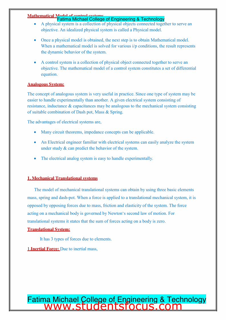
It has 3 types of forces due to elements. 1.Inertial Force: Due to inertial mass,
9 Fatima Michael College of Engineering & Technology
Fatima Michael College of Engineering & Technology
www.studentsfocus.com
Force balance equations of idealized elements
Consider an ideal mass element shown in fig. which has negligible friction and elasticity.
Let a force be applied on it. The mass will offer an opposing force which is proportional to
acceleration of a body.
Let f = applied force
fm =opposing force due to mass d 2 x
Here fm D� M dt 2
ψy Newton‘s second law, f = f m=
d 2 x M
dt 2
2. Damping Force [Viscous Damping]: Due to viscous damping, it is proportional to velocity & is given by,
Damping force is denoted by either D or B or F Consider an ideal frictional element dash-pot shown in fig. which has negligible mass and elasticity. Let a force be applied on it. The dashpot will be offer an opposing force which is proportional to velocity of the body
10 Fatima Michael College of Engineering & Technology
Fatima Michael College of Engineering & Technology
www.studentsfocus.com
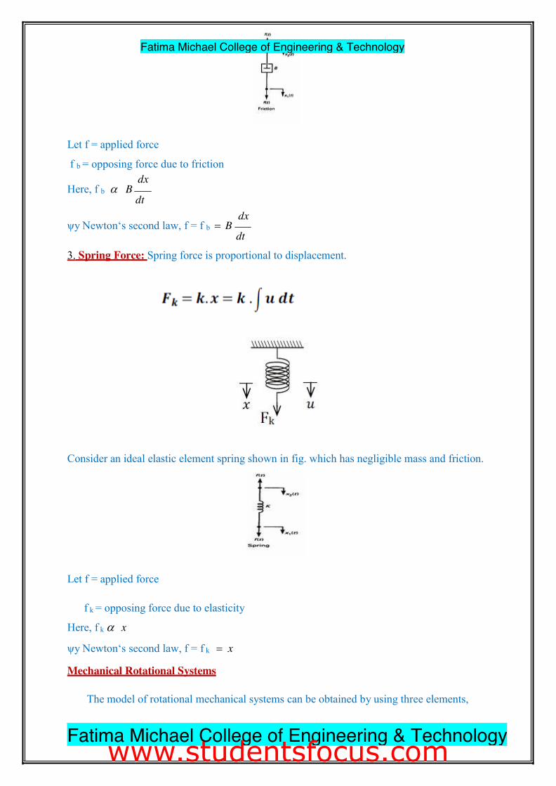
Let f = applied force
f b = opposing force due to friction dx
Here, f b D�� B dt
dx ψy Newton‘s second law, f = f b �B
dt
3. Spring Force: Spring force is proportional to displacement.
Consider an ideal elastic element spring shown in fig. which has negligible mass and friction.
Let f = applied force
f k = opposing force due to elasticity
Here, f k D��x
ψy Newton‘s second law, f = f k � x
Mechanical Rotational Systems
The model of rotational mechanical systems can be obtained by using three elements,
11 Fatima Michael College of Engineering & Technology
Fatima Michael College of Engineering & Technology
www.studentsfocus.com
12
moment of inertia [J] of mass, dash pot with rotational frictional coefficient [B] and torsional
spring with stiffness[k].When a torque is applied to a rotational mechanical system, it is
opposed by opposing torques due to moment of inertia, friction and elasticity of the system.
The torque acting on rotational mechanical bodies is governed by Newton‘s second law of
motion for rotational systems.
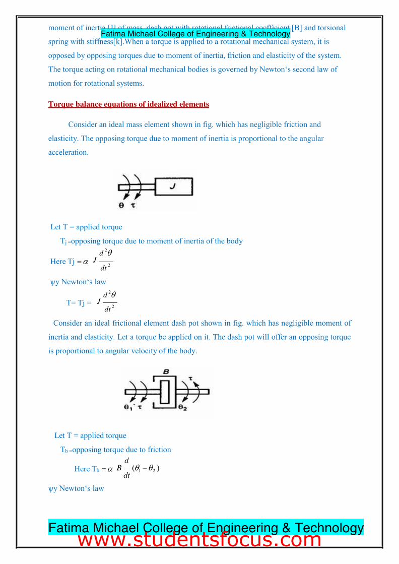
Torque balance equations of idealized elements
Consider an ideal mass element shown in fig. which has negligible friction and
elasticity. The opposing torque due to moment of inertia is proportional to the angular
acceleration.
Let T = applied torque
Tj =opposing torque due to moment of inertia of the body d 2T�
Here Tj �D� J dt 2
ψy Newton‘s law d 2T�
T= Tj = J dt 2
Consider an ideal frictional element dash pot shown in fig. which has negligible moment of
inertia and elasticity. Let a torque be applied on it. The dash pot will offer an opposing torque
is proportional to angular velocity of the body.
Let T = applied torque
Tb =opposing torque due to friction d
Here Tb �D��ψy Newton‘s law
B (T1 ��T2 ) dt
Fatima Michael College of Engineering & Technology
Fatima Michael College of Engineering & Technology
www.studentsfocus.com
13
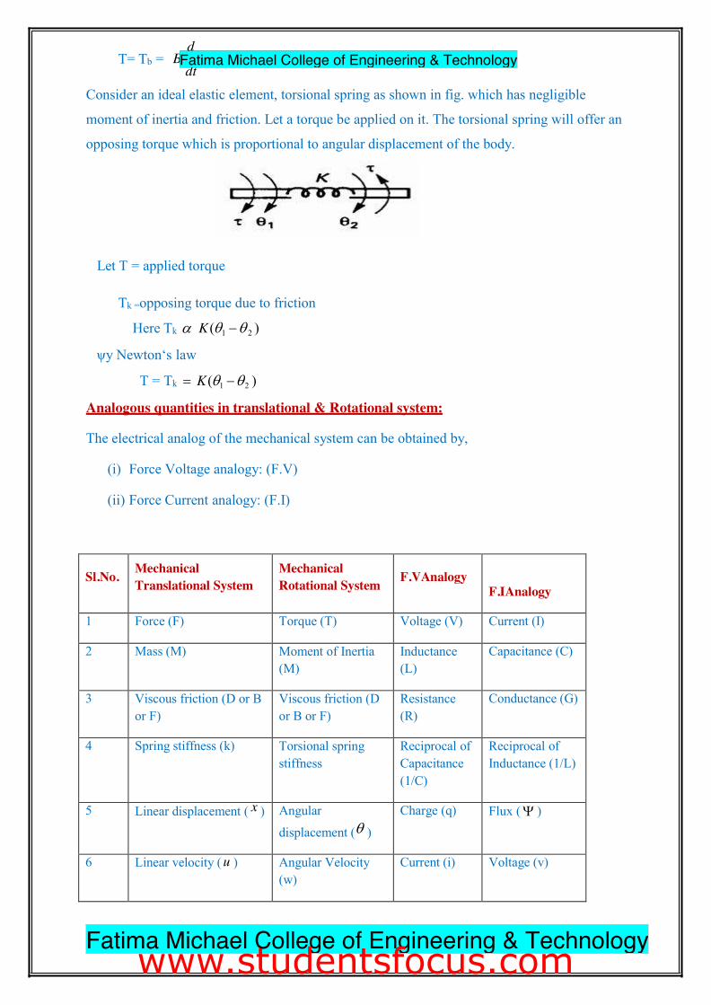
T= Tb = d
B (T1 ��T�2 ) dt
Consider an ideal elastic element, torsional spring as shown in fig. which has negligible
moment of inertia and friction. Let a torque be applied on it. The torsional spring will offer an
opposing torque which is proportional to angular displacement of the body.
Let T = applied torque
Tk =opposing torque due to friction
Here Tk D�
ψy Newton‘s law
K (T1 ��T�2 )
T = Tk �K (T1 ��T2 )
Analogous quantities in translational & Rotational system:
The electrical analog of the mechanical system can be obtained by,
(i) Force Voltage analogy: (F.V)
(ii) Force Current analogy: (F.I)
Sl.No. Mechanical
Translational System Mechanical Rotational System
F.VAnalogy
F.IAnalogy
1 Force (F) Torque (T) Voltage (V) Current (I)
2 Mass (M) Moment of Inertia (M)
Inductance (L)
Capacitance (C)
3 Viscous friction (D or B or F)
Viscous friction (D or B or F)
Resistance (R)
Conductance (G)
4 Spring stiffness (k) Torsional spring stiffness
Reciprocal of Capacitance (1/C)
Reciprocal of Inductance (1/L)
5 Linear displacement ( x ) Angular
displacement (T�) Charge (q) Flux ( <�)
6 Linear velocity ( u ) Angular Velocity (w)
Current (i) Voltage (v)
Fatima Michael College of Engineering & Technology
Fatima Michael College of Engineering & Technology
www.studentsfocus.com
14
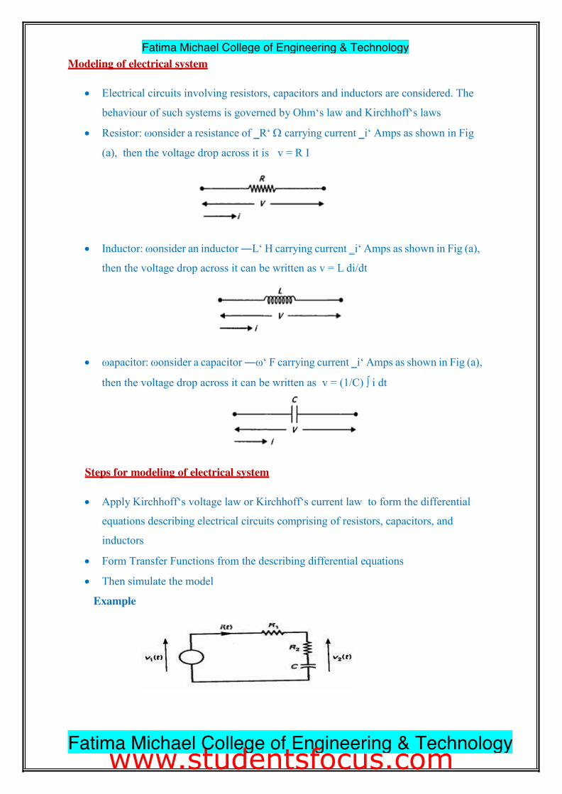
Modeling of electrical system
x Electrical circuits involving resistors, capacitors and inductors are considered. The
behaviour of such systems is governed by Ohm‘s law and Kirchhoff‘s laws
x Resistor: ωonsider a resistance of ‗R‘ :�carrying current ‗i‘ Amps as shown in Fig
(a), then the voltage drop across it is v = R I
x Inductor: ωonsider an inductor ―L‘ H carrying current ‗i‘ Amps as shown in Fig (a),
then the voltage drop across it can be written as v = L di/dt
x ωapacitor: ωonsider a capacitor ―ω‘ F carrying current ‗i‘ Amps as shown in Fig (a),
then the voltage drop across it can be written as v = (1/C) ³�i dt
Steps for modeling of electrical system
x Apply Kirchhoff‘s voltage law or Kirchhoff‘s current law to form the differential
equations describing electrical circuits comprising of resistors, capacitors, and
inductors
x Form Transfer Functions from the describing differential equations
x Then simulate the model
Example
Fatima Michael College of Engineering & Technology
Fatima Michael College of Engineering & Technology
www.studentsfocus.com
c
2
R i(t) ��R i(t) ��1 t i(t)dt �v (t) 1 2 ³ 1
0 t
R i(t) ��1 ³ i(t)dt �v2 (t) c 0
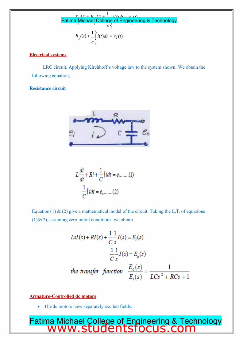
Electrical systems
LRC circuit. Applying Kirchhoff‘s voltage law to the system shown. We obtain the
following equation;
Resistance circuit
Equation (1) & (2) give a mathematical model of the circuit. Taking the L.T. of equations
(1)&(2), assuming zero initial conditions, we obtain
Armature-Controlled dc motors
x The dc motors have separately excited fields.
15 Fatima Michael College of Engineering & Technology
Fatima Michael College of Engineering & Technology
www.studentsfocus.com
x They are either armature-controlled with fixed field or field-controlled with fixed
armature current.
x For example, dc motors used in instruments employ a fixed permanent-magnet field,
and the controlled signal is applied to the armature terminals.
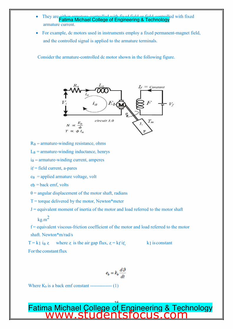
Consider the armature-controlled dc motor shown in the following figure.
Ra = armature-winding resistance, ohms
La = armature-winding inductance, henrys
ia = armature-winding current, amperes
if = field current, a-pares
ea = applied armature voltage, volt
eb = back emf, volts
θ = angular displacement of the motor shaft, radians
T = torque delivered by the motor, Newton*meter
J = equivalent moment of inertia of the motor and load referred to the motor shaft
kg.m2 f = equivalent viscous-friction coefficient of the motor and load referred to the motor
shaft. Newton*m/rad/s
T = k1 ia ȥ where ȥ is the air gap flux, ȥ = kf if, k1 is constant
For the constant flux
Where Kb is a back emf constant -------------- (1)
16 Fatima Michael College of Engineering & Technology
Fatima Michael College of Engineering & Technology
www.studentsfocus.com
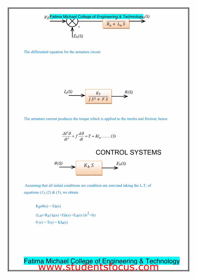
The differential equation for the armature circuit
The armature current produces the torque which is applied to the inertia and friction; hence
CONTROL SYSTEMS
Assuming that all initial conditions are condition are zero/and taking the L.T. of
equations (1), (2) & (3), we obtain
Kpsθ(s) = Eb(s)
(Las+Ra) Ia(s) +Eb(s) =Ea(s) (Js2+fs)
θ (s) = T(s) = KIa(s)
17 Fatima Michael College of Engineering & Technology
Fatima Michael College of Engineering & Technology
www.studentsfocus.com
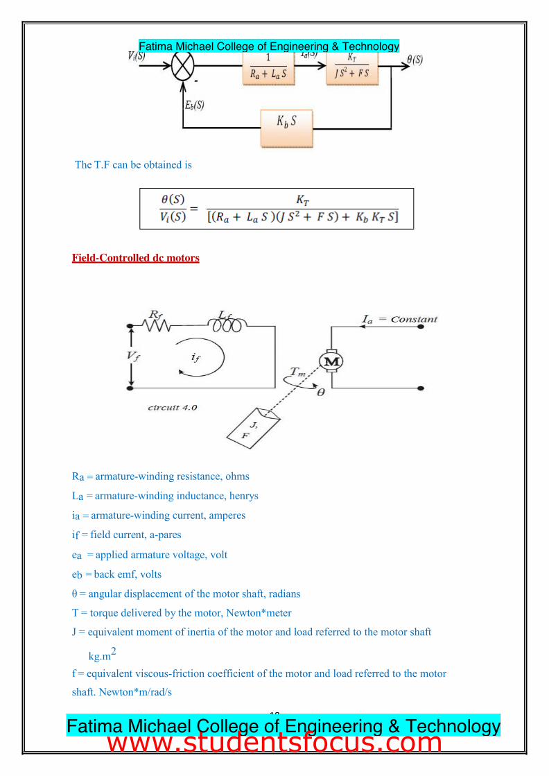
The T.F can be obtained is
Field-Controlled dc motors
Ra = armature-winding resistance, ohms
La = armature-winding inductance, henrys
ia = armature-winding current, amperes
if = field current, a-pares
ea = applied armature voltage, volt
eb = back emf, volts
θ = angular displacement of the motor shaft, radians
T = torque delivered by the motor, Newton*meter
J = equivalent moment of inertia of the motor and load referred to the motor shaft
kg.m2 f = equivalent viscous-friction coefficient of the motor and load referred to the motor
shaft. Newton*m/rad/s
18 Fatima Michael College of Engineering & Technology
Fatima Michael College of Engineering & Technology
www.studentsfocus.com
T = k1 ia ȥ where ȥ is the air gap flux, ȥ = kf if , k1 is constant
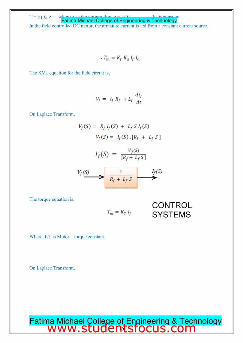
In the field controlled DC motor, the armature current is fed from a constant current source.
The KVL equation for the field circuit is,
On Laplace Transform, The torque equation is,
CONTROL SYSTEMS
Where, KT is Motor – torque constant.
On Laplace Transform,
19 Fatima Michael College of Engineering & Technology
Fatima Michael College of Engineering & Technology
www.studentsfocus.com
2
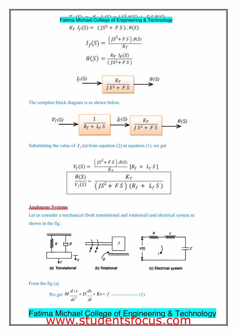
The complete block diagram is as shown below,
Substituting the value of I f (s) from equation (2) in equation (1), we get
Analogous Systems
Let us consider a mechanical (both translational and rotational) and electrical system as
shown in the fig.
From the fig (a)
We get M d x
��D dx ��Kx � f
----------------- (1)
dt 2 dt
20 Fatima Michael College of Engineering & Technology
Fatima Michael College of Engineering & Technology
www.studentsfocus.com
2
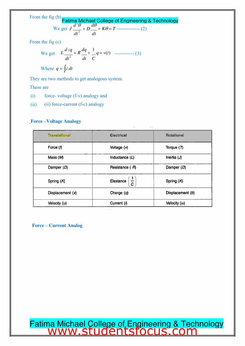
From the fig (b)
We get d 2T dT�
J ��D ��KT� �T -------------- (2) From the fig (c)
dt 2 dt
We get L d q
��R dq ��
1 q �v(t)
------------ (3) dt 2
Where q �³i dt
dt C
They are two methods to get analogous system.
These are
(i) force- voltage (f-v) analogy and
(ii) (ii) force-current (f-c) analogy
Force –Voltage Analogy
Force – Current Analog
21 Fatima Michael College of Engineering & Technology
Fatima Michael College of Engineering & Technology
www.studentsfocus.com
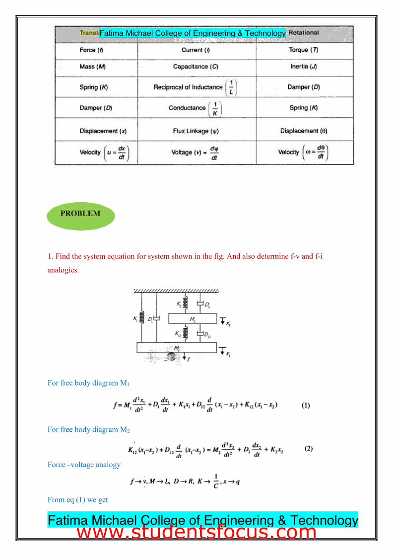
1. Find the system equation for system shown in the fig. And also determine f-v and f-i
analogies.
For free body diagram M1
For free body diagram M2
Force –voltage analogy
From eq (1) we get
22
PROBLEM
Fatima Michael College of Engineering & Technology
Fatima Michael College of Engineering & Technology
www.studentsfocus.com
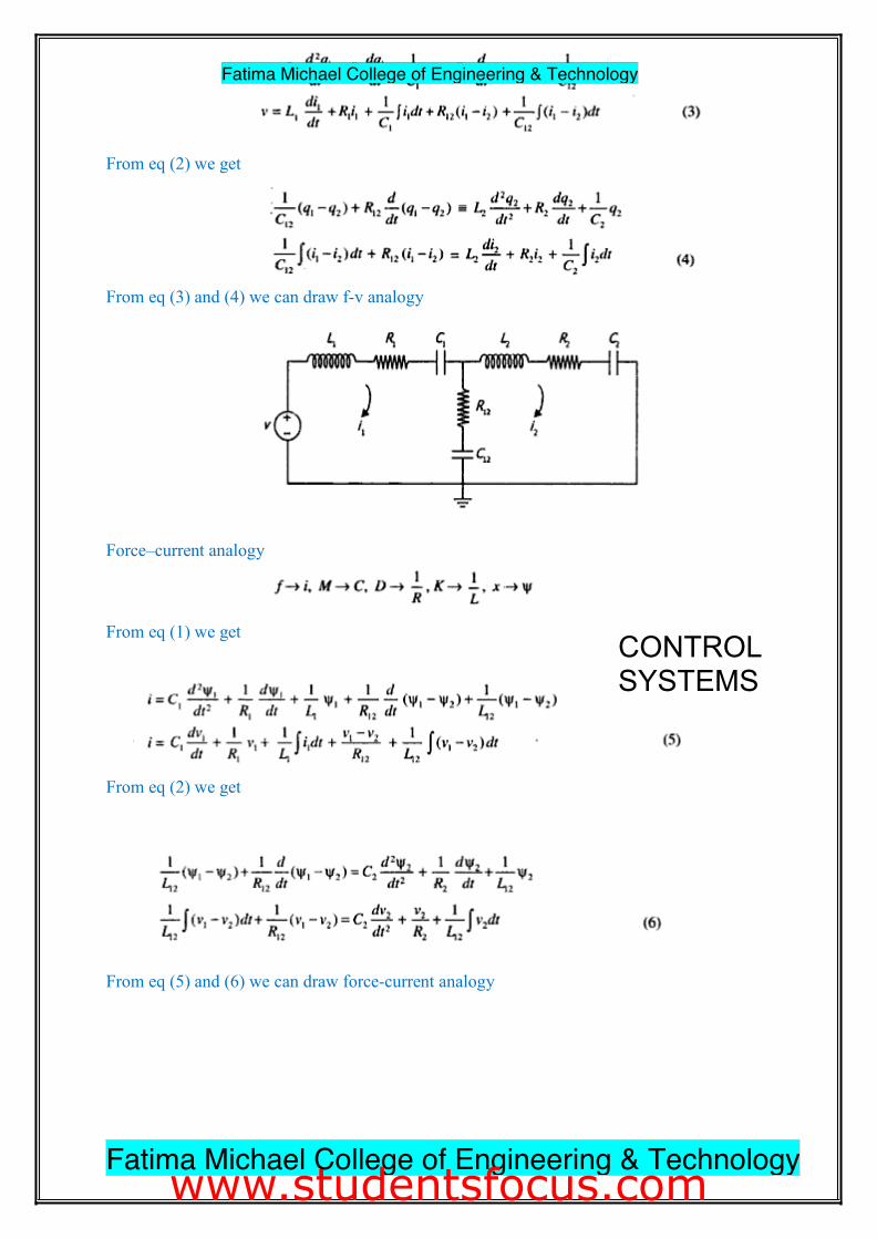
From eq (2) we get
From eq (3) and (4) we can draw f-v analogy Force–current analogy
From eq (1) we get
From eq (2) we get
CONTROL SYSTEMS
From eq (5) and (6) we can draw force-current analogy
23 Fatima Michael College of Engineering & Technology
Fatima Michael College of Engineering & Technology
www.studentsfocus.com
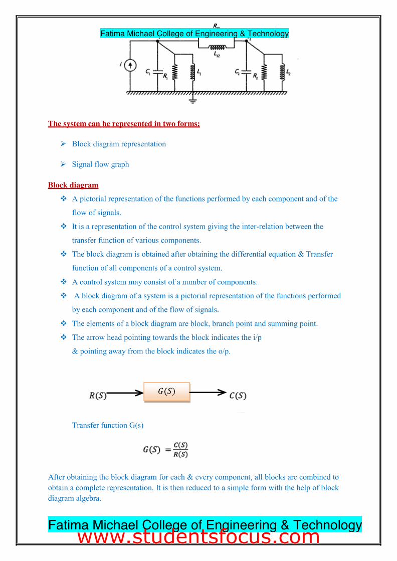
The system can be represented in two forms:
¾ Block diagram representation
¾ Signal flow graph
Block diagram
� A pictorial representation of the functions performed by each component and of the
flow of signals.
� It is a representation of the control system giving the inter-relation between the
transfer function of various components.
� The block diagram is obtained after obtaining the differential equation & Transfer
function of all components of a control system.
� A control system may consist of a number of components.
� A block diagram of a system is a pictorial representation of the functions performed
by each component and of the flow of signals.
� The elements of a block diagram are block, branch point and summing point.
� The arrow head pointing towards the block indicates the i/p
& pointing away from the block indicates the o/p.
Transfer function G(s)
After obtaining the block diagram for each & every component, all blocks are combined to obtain a complete representation. It is then reduced to a simple form with the help of block diagram algebra.
24 Fatima Michael College of Engineering & Technology
Fatima Michael College of Engineering & Technology
www.studentsfocus.com
Basic elements of a block diagram
x Blocks
x Transfer functions of elements inside the blocks
x Summing points
x Take off points
x Arrow
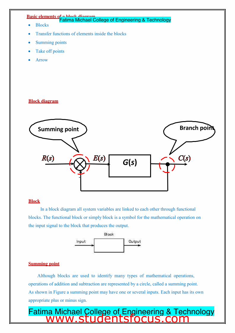
Block diagram
Block
In a block diagram all system variables are linked to each other through functional
blocks. The functional block or simply block is a symbol for the mathematical operation on
the input signal to the block that produces the output.
Summing point
Although blocks are used to identify many types of mathematical operations,
operations of addition and subtraction are represented by a circle, called a summing point.
As shown in Figure a summing point may have one or several inputs. Each input has its own
appropriate plus or minus sign.
25
G(s)
Summing point Branch point
+―
-
Fatima Michael College of Engineering & Technology
Fatima Michael College of Engineering & Technology
www.studentsfocus.com
A summing point has only one output and is equal to the algebraic sum of the
inputs.
A takeoff point is used to allow a signal to be used by more than one block or summing
point.
The transfer function is given inside the block
• The input in this case is E(s)
• The output in this case is ω(s)
• ω(s) = G(s) E(s)
x Functional block – each element of the practical system represented by block with its
T.F.
x Branches – lines showing the connection between the blocks
x Arrow – associated with each branch to indicate the direction of flow of signal
x Closed loop system
x Summing point – comparing the different signals
x Take off point – point from which signal is taken for feed back
Advantages of Block Diagram Representation
x Very simple to construct block diagram for a complicated system
x Function of individual element can be visualized
x Individual & Overall performance can be studied
x Over all transfer function can be calculated easily
26 Fatima Michael College of Engineering & Technology
Fatima Michael College of Engineering & Technology
www.studentsfocus.com
Disadvantages of Block Diagram Representation
x No information about the physical construction
x Source of energy is not shown
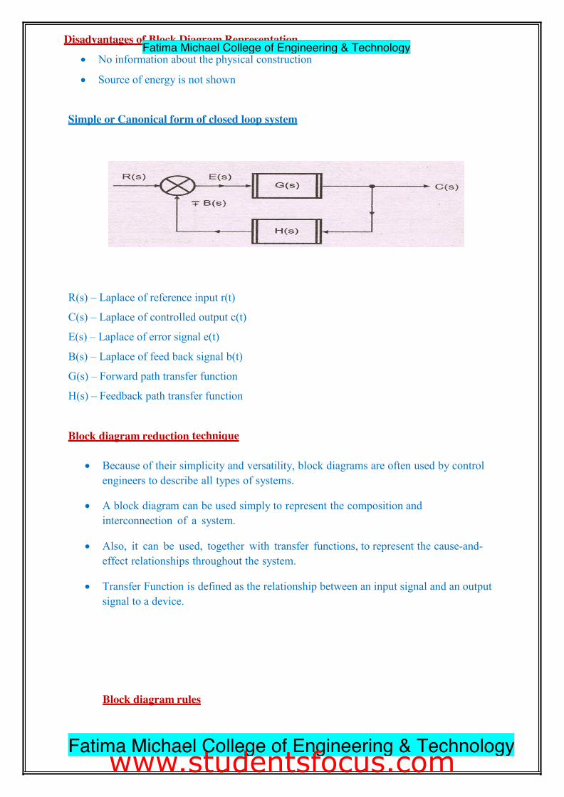
Simple or Canonical form of closed loop system
R(s) – Laplace of reference input r(t)
C(s) – Laplace of controlled output c(t)
E(s) – Laplace of error signal e(t)
B(s) – Laplace of feed back signal b(t)
G(s) – Forward path transfer function
H(s) – Feedback path transfer function
Block diagram reduction technique
x Because of their simplicity and versatility, block diagrams are often used by control engineers to describe all types of systems.
x A block diagram can be used simply to represent the composition and interconnection of a system.
x Also, it can be used, together with transfer functions, to represent the cause-and- effect relationships throughout the system.
x Transfer Function is defined as the relationship between an input signal and an output signal to a device.
Block diagram rules
27 Fatima Michael College of Engineering & Technology
Fatima Michael College of Engineering & Technology
www.studentsfocus.com
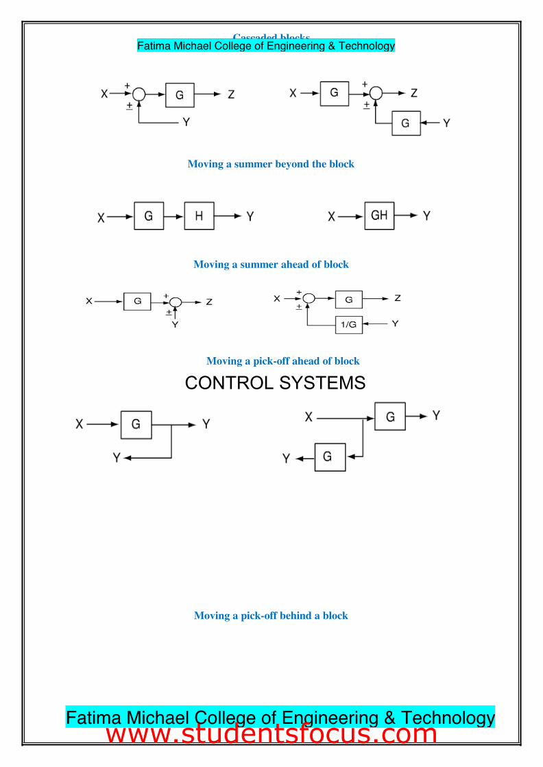
Cascaded blocks
Moving a summer beyond the block
Moving a summer ahead of block
Moving a pick-off ahead of block
CONTROL SYSTEMS
Moving a pick-off behind a block
28 Fatima Michael College of Engineering & Technology
Fatima Michael College of Engineering & Technology
www.studentsfocus.com
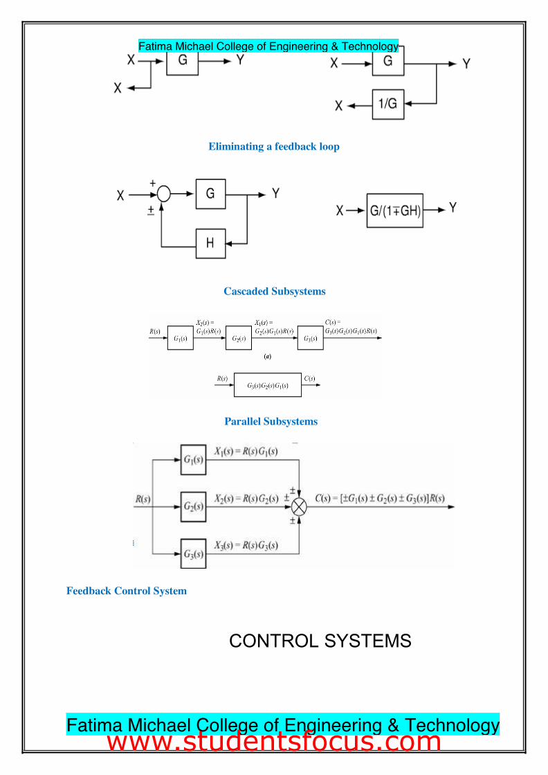
Feedback Control System
Eliminating a feedback loop
Cascaded Subsystems
Parallel Subsystems
CONTROL SYSTEMS
29 Fatima Michael College of Engineering & Technology
Fatima Michael College of Engineering & Technology
www.studentsfocus.com
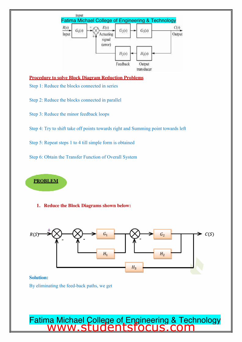
Procedure to solve Block Diagram Reduction Problems
Step 1: Reduce the blocks connected in series
Step 2: Reduce the blocks connected in parallel
Step 3: Reduce the minor feedback loops
Step 4: Try to shift take off points towards right and Summing point towards left
Step 5: Repeat steps 1 to 4 till simple form is obtained
Step 6: Obtain the Transfer Function of Overall System
1. Reduce the Block Diagrams shown below:
Solution: By eliminating the feed-back paths, we get
30
PROBLEM
Fatima Michael College of Engineering & Technology
Fatima Michael College of Engineering & Technology
www.studentsfocus.com
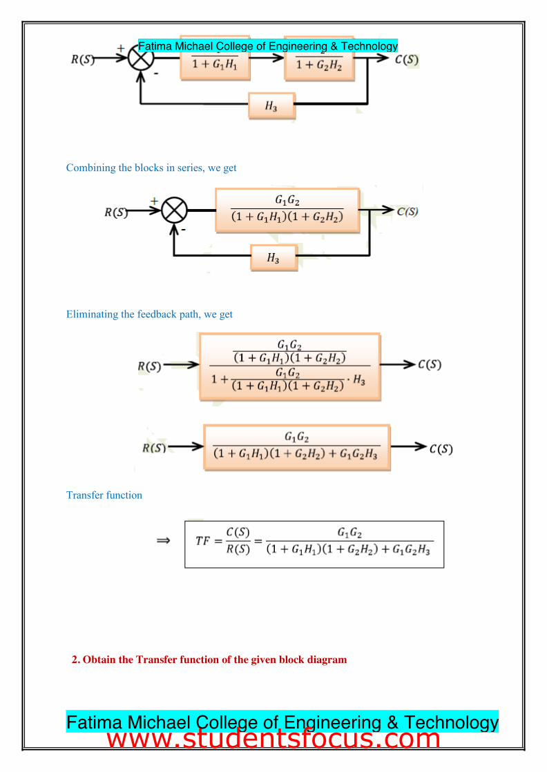
Combining the blocks in series, we get
Eliminating the feedback path, we get
Transfer function
2. Obtain the Transfer function of the given block diagram
31 Fatima Michael College of Engineering & Technology
Fatima Michael College of Engineering & Technology
www.studentsfocus.com
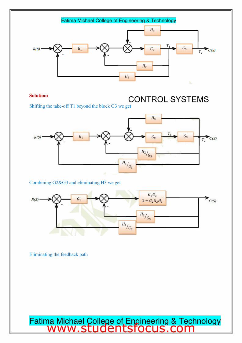
Solution: CONTROL SYSTEMS Shifting the take-off T1 beyond the block G3 we get
Combining G2&G3 and eliminating H3 we get
Eliminating the feedback path
32 Fatima Michael College of Engineering & Technology
Fatima Michael College of Engineering & Technology
www.studentsfocus.com
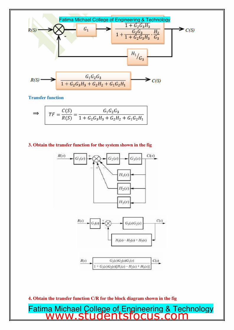
Transfer function
3. Obtain the transfer function for the system shown in the fig
4. Obtain the transfer function C/R for the block diagram shown in the fig
33 Fatima Michael College of Engineering & Technology
Fatima Michael College of Engineering & Technology
www.studentsfocus.com
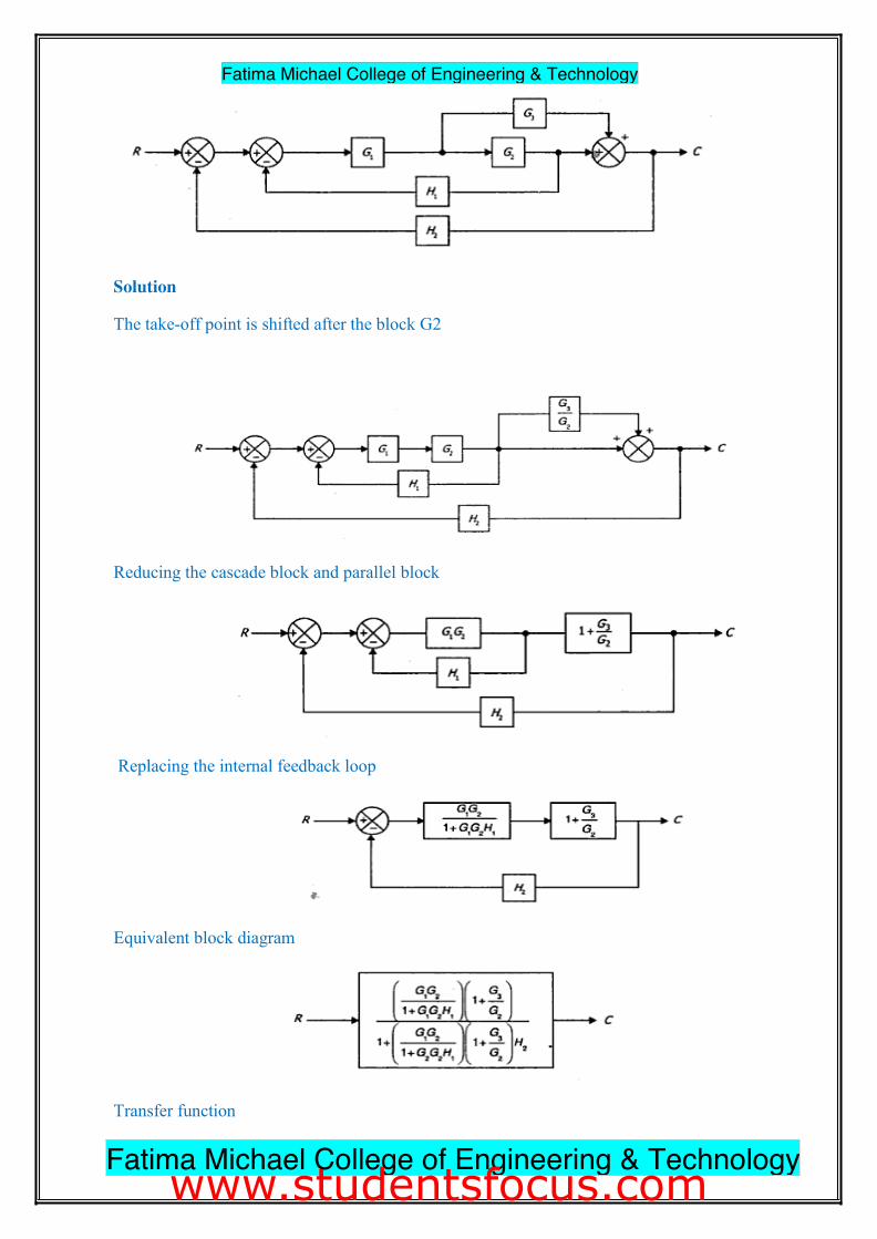
Solution The take-off point is shifted after the block G2
Reducing the cascade block and parallel block
Replacing the internal feedback loop
Equivalent block diagram
Transfer function
34 Fatima Michael College of Engineering & Technology
Fatima Michael College of Engineering & Technology
www.studentsfocus.com
Signal Flow Graph Representation
x Signal Flow Graph Representation of a system obtained from the equations, which
shows the flow of the signal
x For complicated systems, Block diagram reduction method becomes tedious & time consuming. An alternate method is that signal flow graphs developed by S.J. Mason.
x In these graphs, each node represents a system variable & each branch connected between two nodes acts as Signal Multiplier.
x The direction of signal flow is indicated by an arrow.
Signal flow graph
x A signal flow graph is a diagram that represents a set of simultaneous linear
algebraic equations.
x By taking Laplace transfer, the time domain differential equations governing a
control system can be transferred to a set of algebraic equation in s-domain.
x A signal-flow graph consists of a network in which nodes are connected by
directed branches.
x It depicts the flow of signals from one point of a system to another and gives the
relationships among the signals.
Definitions
¾ Node: A node is a point representing a variable.
¾ Transmittance: A transmittance is a gain between two nodes.
¾ Branch: A branch is a line joining two nodes. The signal travels along a branch.
35 Fatima Michael College of Engineering & Technology
Fatima Michael College of Engineering & Technology
www.studentsfocus.com
¾ Input node [Source]: It is a node which has only out going signals.
¾ Output node [Sink]: It is a node which is having only incoming signals.
¾ Mixed node: It is a node which has both incoming & outgoing branches (signals).
¾ Path: It is the traversal of connected branches in the direction of branch arrows. Such that no node is traversed more than once.
¾ Loop: It is a closed path.
¾ Loop Gain: It is the product of the branch transmittances of a loop.
¾ Non-Touching Loops: Loops are Non-Touching, if they do not possess any common node.
¾ Forward Path: It is a path from i/p node to the o/p node w hich doesn‘t cross any node more than once.
¾ Forward Path Gain: It is the product of branch transmittances of a forward path.
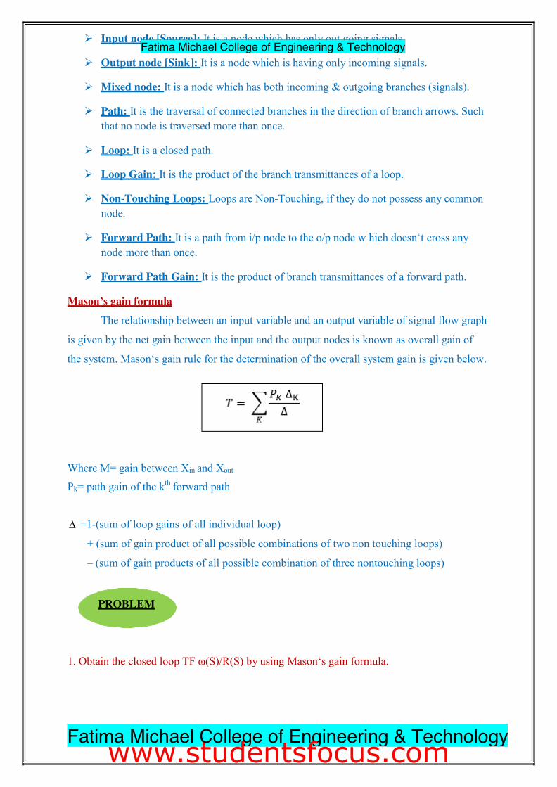
Mason’s gain formula
The relationship between an input variable and an output variable of signal flow graph
is given by the net gain between the input and the output nodes is known as overall gain of
the system. Mason‘s gain rule for the determination of the overall system gain is given below.
Where M= gain between Xin and Xout
Pk= path gain of the kth forward path
'�=1-(sum of loop gains of all individual loop)
+ (sum of gain product of all possible combinations of two non touching loops)
– (sum of gain products of all possible combination of three nontouching loops)
1. Obtain the closed loop TF ω(S)/R(S) by using Mason‘s gain formula.
36
PROBLEM
Fatima Michael College of Engineering & Technology
Fatima Michael College of Engineering & Technology
www.studentsfocus.com
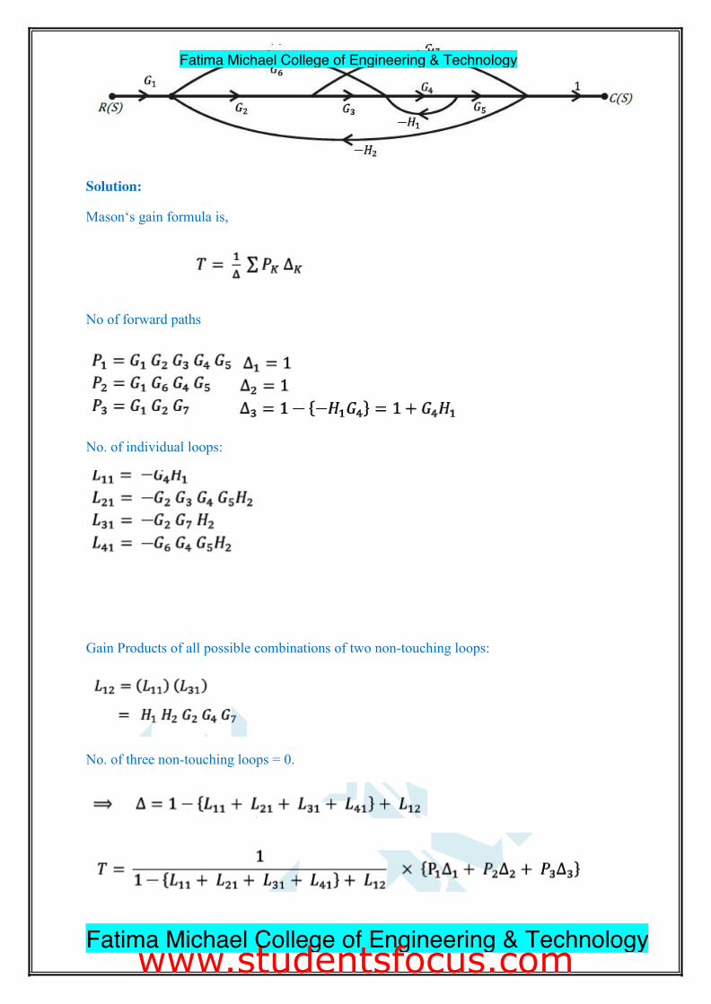
Solution: Mason‘s gain formula is,
No of forward paths
No. of individual loops:
Gain Products of all possible combinations of two non-touching loops:
No. of three non-touching loops = 0.
37 Fatima Michael College of Engineering & Technology
Fatima Michael College of Engineering & Technology
www.studentsfocus.com
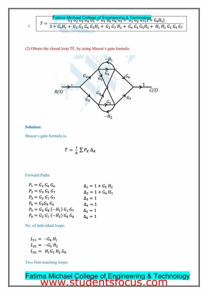
(2) Obtain the closed loop TF, by using Mason‘s gain formula.
Solution:
Mason‘s gain formula is,
Forward Paths:
No. of individual loops:
Two Non-touching loops:
38 Fatima Michael College of Engineering & Technology
Fatima Michael College of Engineering & Technology
www.studentsfocus.com
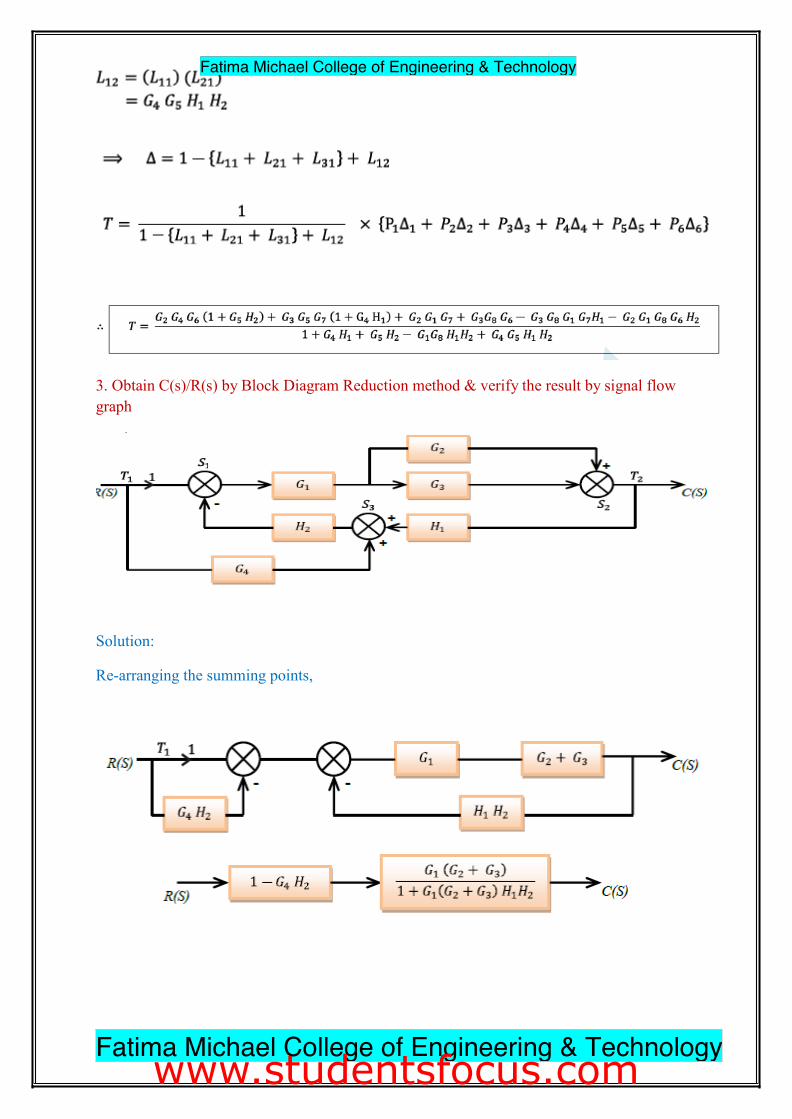
3. Obtain C(s)/R(s) by Block Diagram Reduction method & verify the result by signal flow graph
Solution:
Re-arranging the summing points,
39 Fatima Michael College of Engineering & Technology
Fatima Michael College of Engineering & Technology
www.studentsfocus.com

Signal flow graphs:
No. of forward paths:
No. of individual loops:
Mason‘s gain formula is,
Modeling of Elements of Control Systems
A feedback control system usually consists of several components in addition to the actual process. These are error detectors, power amplifiers, actuators, sensors etc. Let us now discuss the physical characteristics of some of these and obtain their mathematical models.
DC Servo Motor
x A DC servo motor is used as an actuator to drive a load. It is usually a DC motor of low power rating.
40 Fatima Michael College of Engineering & Technology
Fatima Michael College of Engineering & Technology
www.studentsfocus.com
x DC servo motors have a high ratio of starting torque to inertia and therefore they have a faster dynamic response.
x DC motors are constructed using rare earth permanent magnets which have high residual flux density and high coercively.
x As no field winding is used, the field copper losses am zero and hence, the overall efficiency of the motor is high.
x The speed torque characteristic of this motor is flat over a wide range, as the armature reaction is negligible.
x Moreover speed in directly proportional to the armature voltage for a given torque. Armature of a DC servo motor is specially designed to have low inertia.
x In some application DC servo motors are used with magnetic flux produced by field windings.
x The speed of PMDC motors can be controlled by applying variable armature voltage. These are called armature voltage controlled DC servo motors.
x Wound field DC motors can be controlled by either controlling the armature voltage or controlling rho field current. Let us now consider modelling of these two types or DC servo motors.
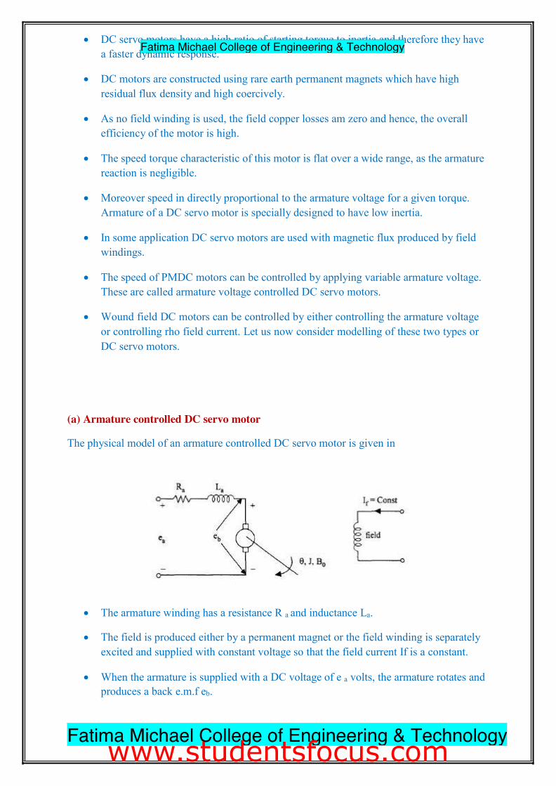
(a) Armature controlled DC servo motor
The physical model of an armature controlled DC servo motor is given in
x The armature winding has a resistance R a and inductance La.
x The field is produced either by a permanent magnet or the field winding is separately excited and supplied with constant voltage so that the field current If is a constant.
x When the armature is supplied with a DC voltage of e a volts, the armature rotates and produces a back e.m.f eb.
41 Fatima Michael College of Engineering & Technology
Fatima Michael College of Engineering & Technology
www.studentsfocus.com
x The armature current ia depends on the difference of eb and en. The armature has a remnant of inertia J, frictional coefficient B0
x The angular displacement of the motor is 8.
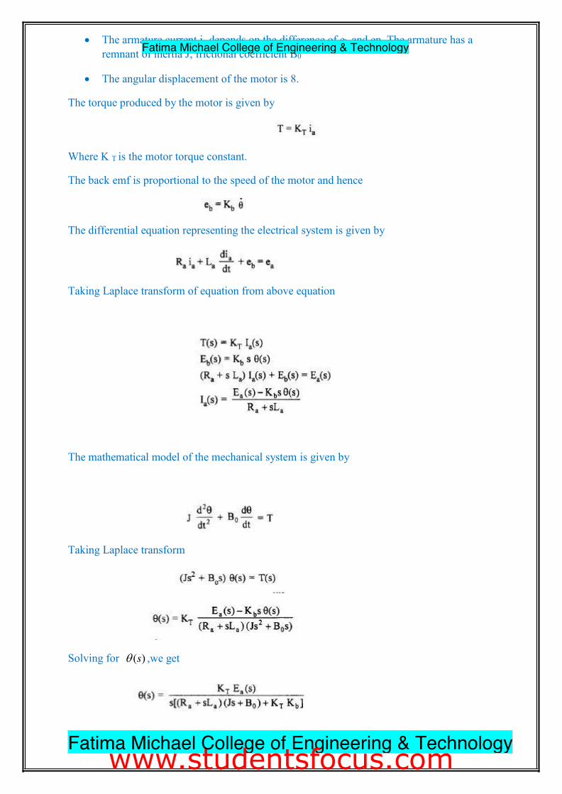
The torque produced by the motor is given by
Where K T is the motor torque constant.
The back emf is proportional to the speed of the motor and hence
The differential equation representing the electrical system is given by
Taking Laplace transform of equation from above equation
The mathematical model of the mechanical system is given by
Taking Laplace transform
Solving for T�(s) ,we get
42 Fatima Michael College of Engineering & Technology
Fatima Michael College of Engineering & Technology
www.studentsfocus.com
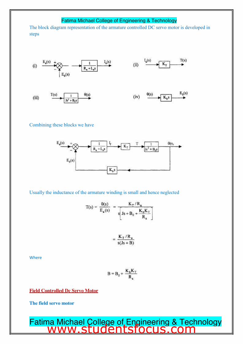
The block diagram representation of the armature controlled DC servo motor is developed in steps
Combining these blocks we have
Usually the inductance of the armature winding is small and hence neglected
Where
Field Controlled Dc Servo Motor
The field servo motor
43 Fatima Michael College of Engineering & Technology
Fatima Michael College of Engineering & Technology
www.studentsfocus.com
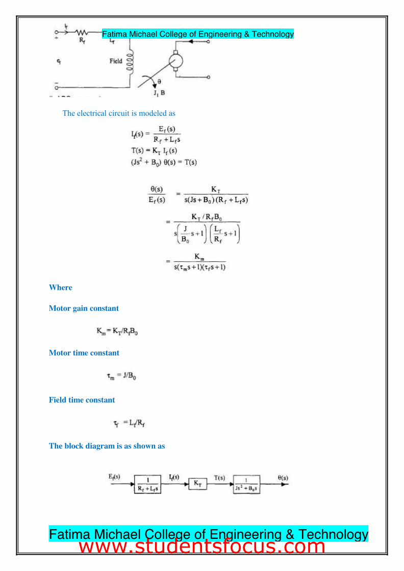
The electrical circuit is modeled as
Where
Motor gain constant
Motor time constant
Field time constant
The block diagram is as shown as
44 Fatima Michael College of Engineering & Technology
Fatima Michael College of Engineering & Technology
www.studentsfocus.com
AC Servo Motors
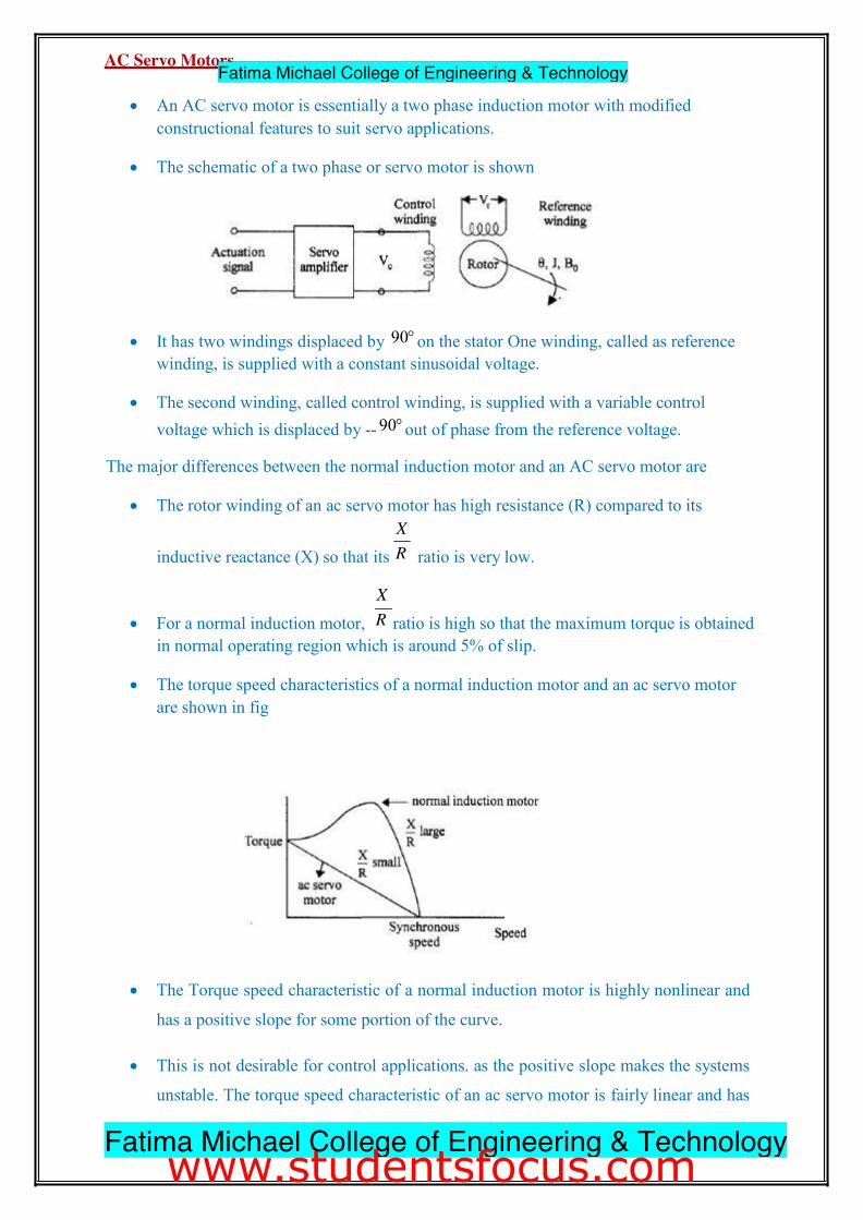
x An AC servo motor is essentially a two phase induction motor with modified constructional features to suit servo applications.
x The schematic of a two phase or servo motor is shown
x It has two windings displaced by 90qon the stator One winding, called as reference winding, is supplied with a constant sinusoidal voltage.
x The second winding, called control winding, is supplied with a variable control voltage which is displaced by -- 90qout of phase from the reference voltage.
The major differences between the normal induction motor and an AC servo motor are
x The rotor winding of an ac servo motor has high resistance (R) compared to its X
inductive reactance (X) so that its R ratio is very low.
X
x For a normal induction motor, R ratio is high so that the maximum torque is obtained in normal operating region which is around 5% of slip.
x The torque speed characteristics of a normal induction motor and an ac servo motor are shown in fig
x The Torque speed characteristic of a normal induction motor is highly nonlinear and
has a positive slope for some portion of the curve.
x This is not desirable for control applications. as the positive slope makes the systems
unstable. The torque speed characteristic of an ac servo motor is fairly linear and has
45 Fatima Michael College of Engineering & Technology
Fatima Michael College of Engineering & Technology
www.studentsfocus.com
negative slope throughout.
x The rotor construction is usually squirrel cage or drag cup type for an ac servo motor.
The diameter is small compared to the length of the rotor which reduces inertia of the
moving parts.
x Thus it has good accelerating characteristic and good dynamic response.
x The supplies to the two windings of ac servo motor are not balanced as in the case of
a normal induction motor.
x The control voltage varies both in magnitude and phase with respect to the constant
reference vulture applied to the reference winding.
x The direction of rotation of the motor depends on the phase (± 90°) of the control
voltage with respect to the reference voltage.
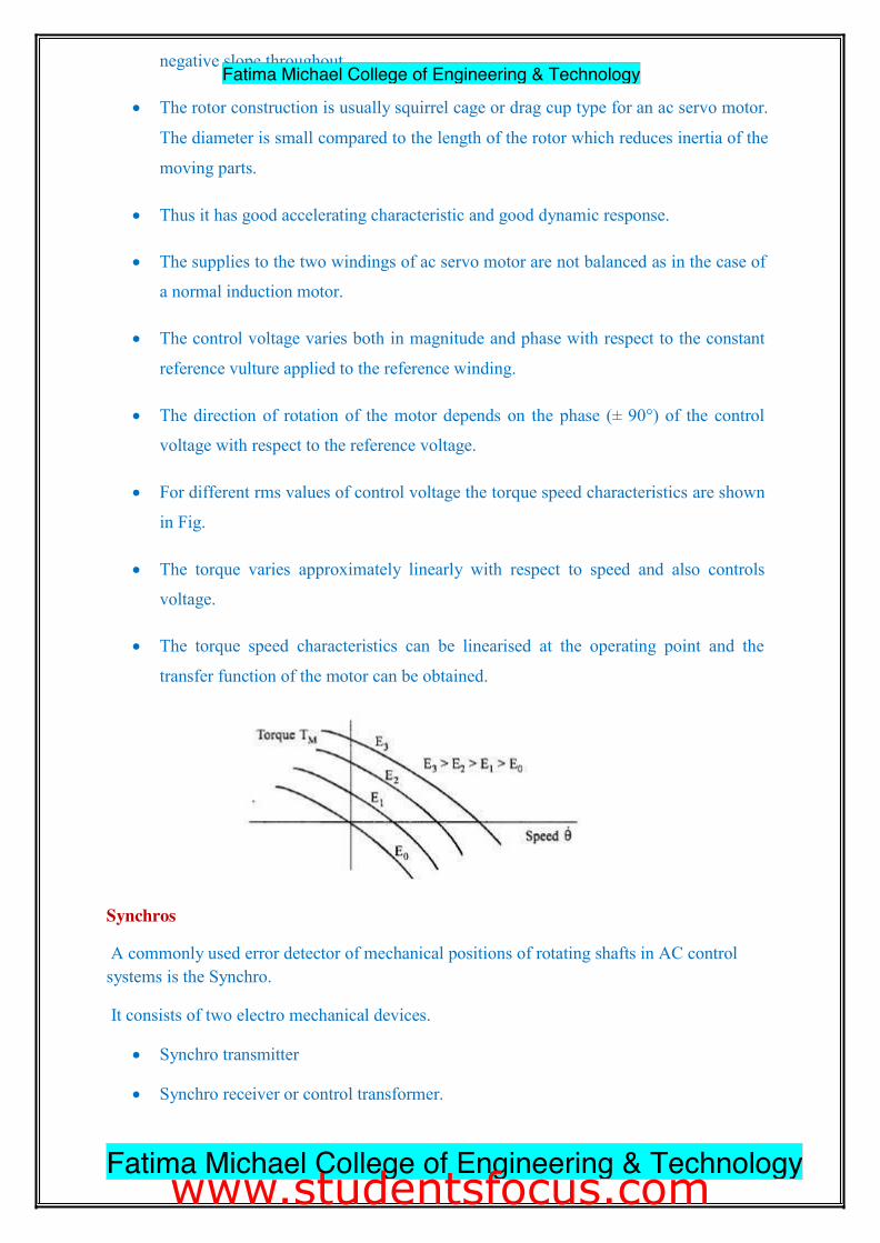
x For different rms values of control voltage the torque speed characteristics are shown
in Fig.
x The torque varies approximately linearly with respect to speed and also controls
voltage.
x The torque speed characteristics can be linearised at the operating point and the
transfer function of the motor can be obtained.
Synchros
A commonly used error detector of mechanical positions of rotating shafts in AC control systems is the Synchro.
It consists of two electro mechanical devices.
x Synchro transmitter
x Synchro receiver or control transformer.
46 Fatima Michael College of Engineering & Technology
Fatima Michael College of Engineering & Technology
www.studentsfocus.com
The principle of operation of these two devices is sarne but they differ slightly in their construction.
x The construction of a Synchro transmitter is similar to a phase alternator.
x The stator consists of a balanced three phase winding and is star connected.
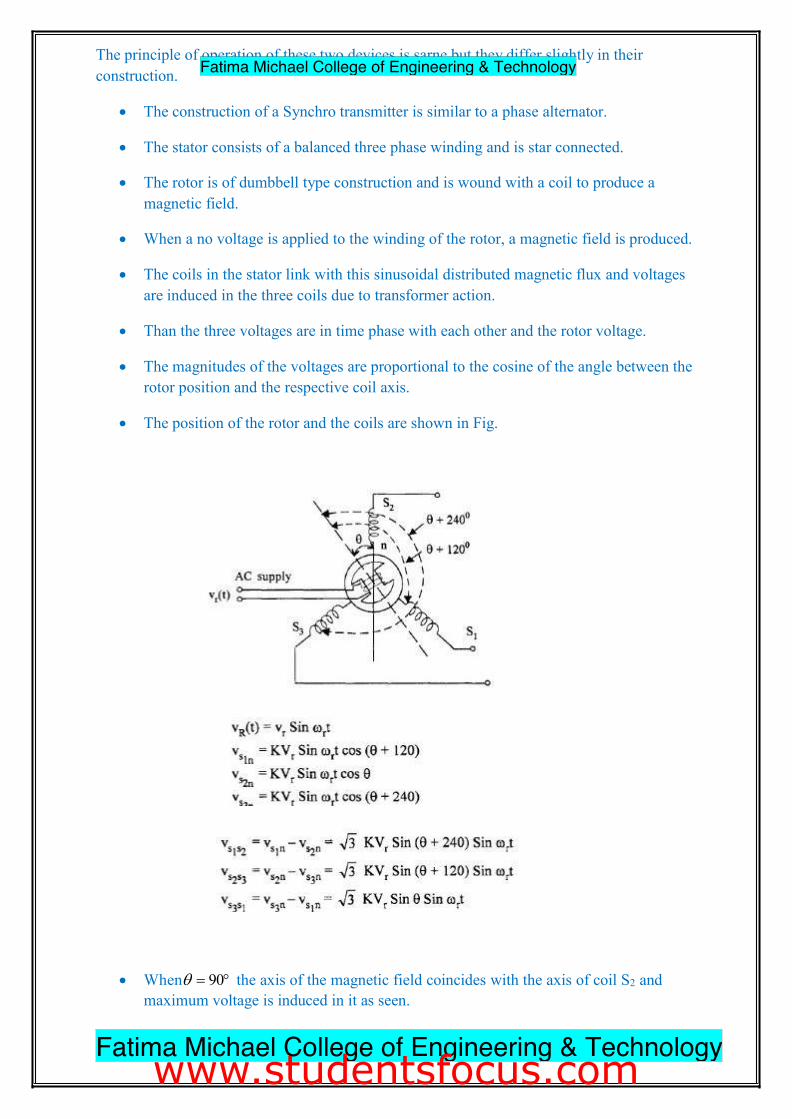
x The rotor is of dumbbell type construction and is wound with a coil to produce a magnetic field.
x When a no voltage is applied to the winding of the rotor, a magnetic field is produced.
x The coils in the stator link with this sinusoidal distributed magnetic flux and voltages are induced in the three coils due to transformer action.
x Than the three voltages are in time phase with each other and the rotor voltage.
x The magnitudes of the voltages are proportional to the cosine of the angle between the rotor position and the respective coil axis.
x The position of the rotor and the coils are shown in Fig.
x WhenT� �90q� the axis of the magnetic field coincides with the axis of coil S2 and maximum voltage is induced in it as seen.
47 Fatima Michael College of Engineering & Technology
Fatima Michael College of Engineering & Technology
www.studentsfocus.com
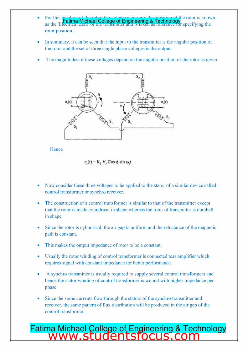
x For this position of the rotor, the voltage c, is zero, this position of the rotor is known as the 'Electrical Zero' of die transmitter and is taken as reference for specifying the rotor position.
x In summary, it can be seen that the input to the transmitter is the angular position of the rotor and the set of three single phase voltages is the output.
x The magnitudes of these voltages depend on the angular position of the rotor as given
Hence
x Now consider these three voltages to he applied to the stator of a similar device called control transformer or synchro receiver.
x The construction of a control transformer is similar to that of the transmitter except that the rotor is made cylindrical in shape whereas the rotor of transmitter is dumbell in shape.
x Since the rotor is cylindrical, the air gap is uniform and the reluctance of the magnetic path is constant.
x This makes the output impedance of rotor to be a constant. x Usually the rotor winding of control transformer is connected teas amplifier which
requires signal with constant impedance for better performance.
x A synchro transmitter is usually required to supply several control transformers and hence the stator winding of control transformer is wound with higher impedance per phase.
x Since the some currents flow through the stators of the synchro transmitter and receiver, the same pattern of flux distribution will be produced in the air gap of the control transformer.
48 Fatima Michael College of Engineering & Technology
Fatima Michael College of Engineering & Technology
www.studentsfocus.com

x The control transformer flux axis is in the same position as that of the synchro transmitter.
x Thus the voltage induced in the rotor coil of control transformer is proportional to the cosine of the angle between the two rotors.
**************************
CONTROL SYSTEM MODELLING
49
UNIT I
Fatima Michael College of Engineering & Technology
Fatima Michael College of Engineering & Technology
www.studentsfocus.com
PART – A 1. What is control system?
2. Define open loop control system.
3. Define closed loop control system.
4. Define transfer function.
5. What are the basic elements used for modeling mechanical rotational system?
6. Name two types of electrical analogous for mechanical system.
7. What is block diagram?
8. What is the basis for framing the rules of block diagram reduction technique?
9. What is a signal flow graph?
10. What is transmittance?
11. What is sink and source?
12. Define non- touching loop.
13. Write Masons Gain formula.
14. Write the analogous electrical elements in force voltage analogy for the elements of
mechanical translational system.
15. Write the analogous electrical elements in force current analogy for the elements of
mechanical translational system.
16. Write the force balance equation of m ideal mass element.
17. Write the force balance equation of ideal dashpot element.
18. Write the force balance equation of ideal spring element.
19. What is servomechanism?
PART – B
1. Write the differential equations governing the Mechanical system shown in fig.
and determine the transfer function. (16)
2. Determine the transfer function Y2(S)/F(S) of the system shown in fig. (16)
50 Fatima Michael College of Engineering & Technology
Fatima Michael College of Engineering & Technology
www.studentsfocus.com

![INDEX [studentsfocus.com]studentsfocus.com/notes/anna_university/IT/4SEM... · cs6412 – microprocessor and microcontroller lab dept of cse 2 expt.no name of the experiment page](https://static.fdocuments.net/doc/165x107/5afd184c7f8b9a323491255e/index-microprocessor-and-microcontroller-lab-dept-of-cse-2-exptno-name.jpg)


