Hyperspectral Remote Sensing of Vegetation Remote Sensing of Vegetation Definition of Hyperspectral...
77
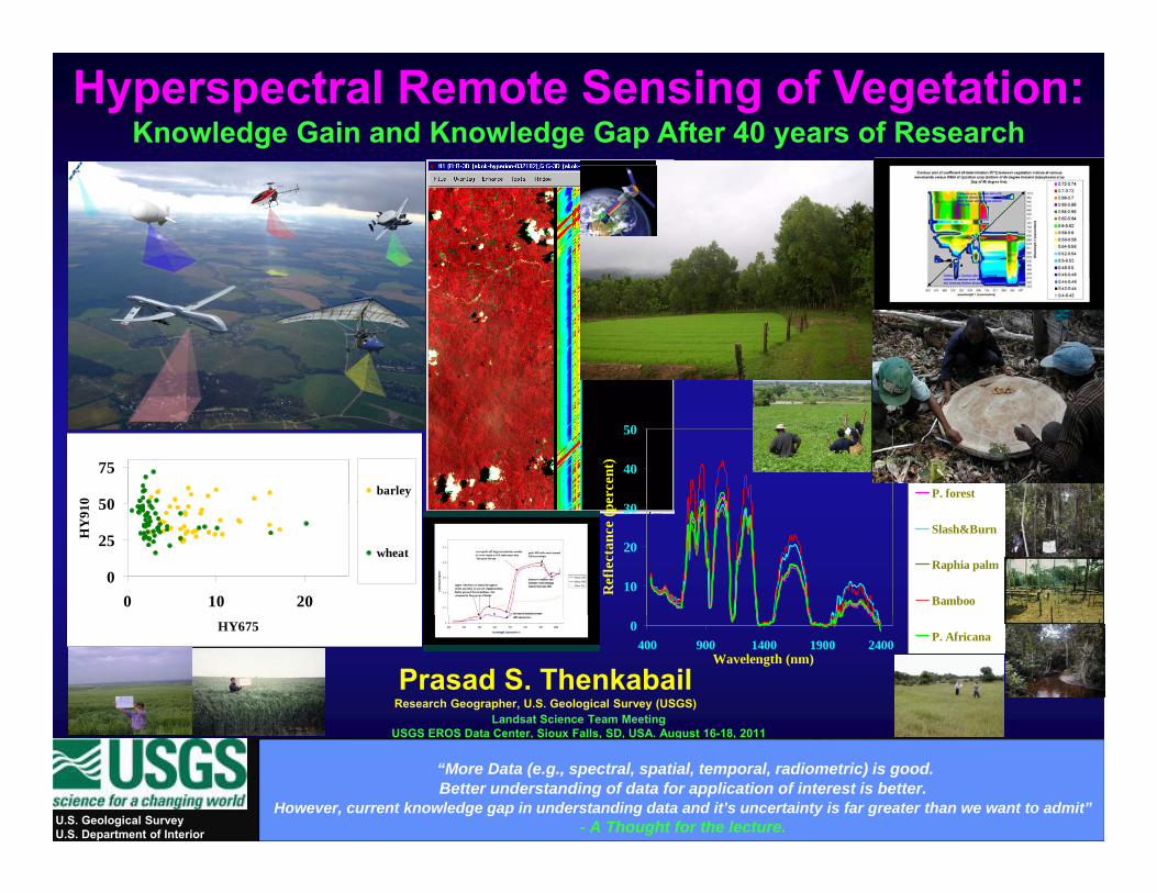
Hyperspectral Remote Sensing of Vegetation: Knowledge Gain and Knowledge Gap After 40 years of Research 40 50 ercent) Y. sec. Forest P. forest 50 75 0 barley 10 20 30 Reflectance (pe Slash&Burn Raphia palm Bamboo 0 25 50 0 10 20 HY910 wheat Prasad S. Thenkabail Research Geographer, U.S. Geological Survey (USGS) Landsat Science Team Meeting 0 400 900 1400 1900 2400 Wavelength (nm) P. Africana HY675 U.S. Geological Survey U.S. Department of Interior USGS EROS Data Center, Sioux Falls, SD, USA. August 16-18, 2011 “More Data (e.g., spectral, spatial, temporal, radiometric) is good. Better understanding of data for application of interest is better. However, current knowledge gap in understanding data and it’s uncertainty is far greater than we want to admit” - A Thought for the lecture.
Transcript of Hyperspectral Remote Sensing of Vegetation Remote Sensing of Vegetation Definition of Hyperspectral...
Hyperspectral Remote Sensing of Vegetation: Knowledge Gain and Knowledge Gap After 40 years of Research
40
50
erce
nt) Y. sec. Forest
P. forest50
75
0
barley
10
20
30
Ref
lect
ance
(pe
Slash&Burn
Raphia palm
Bamboo
0
25
50
0 10 20
HY
910
wheat
Prasad S. Thenkabail Research Geographer, U.S. Geological Survey (USGS)
Landsat Science Team Meeting
0400 900 1400 1900 2400
Wavelength (nm)
P. AfricanaHY675
U.S. Geological SurveyU.S. Department of Interior
USGS EROS Data Center, Sioux Falls, SD, USA. August 16-18, 2011
“More Data (e.g., spectral, spatial, temporal, radiometric) is good. Better understanding of data for application of interest is better.
However, current knowledge gap in understanding data and it’s uncertainty is far greater than we want to admit”- A Thought for the lecture.
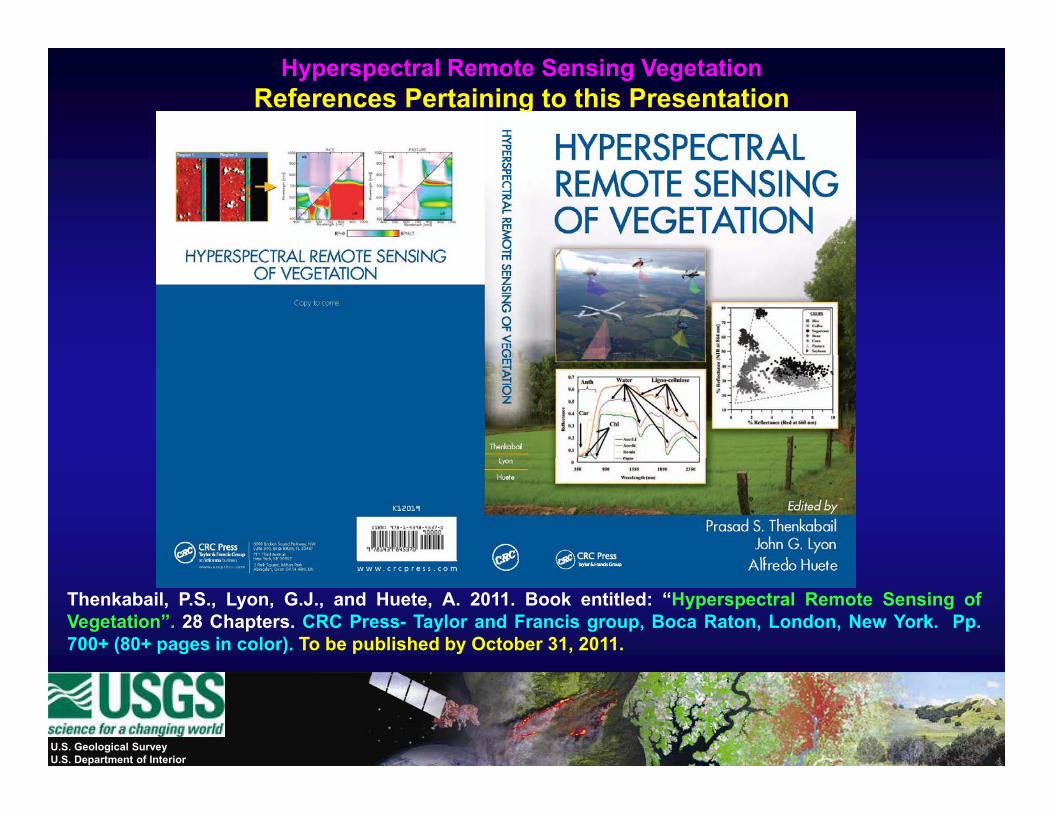
Hyperspectral Remote Sensing Vegetation References Pertaining to this Presentation
Thenkabail, P.S., Lyon, G.J., and Huete, A. 2011. Book entitled: “Hyperspectral Remote Sensing ofVegetation”. 28 Chapters. CRC Press- Taylor and Francis group, Boca Raton, London, New York. Pp.700+ (80+ pages in color). To be published by October 31, 2011.
U.S. Geological SurveyU.S. Department of Interior

Importance of Hyperspectral Sensors (Imaging Spectrometry) inHyperspectral Sensors (Imaging Spectrometry) in
Study of Vegetation
U.S. Geological SurveyU.S. Department of Interior
Hyperspectral Remote Sensing of Vegetation Importance of Hyperspectral Sensors (Imaging Spectroscopy) in Study of Vegetation
More specifically…………..hyperspectral Remote Sensing, originally used for detecting and mapping minerals, is increasingly needed for to characterize, model, classify, and map agricultural crops and , , y, p g pnatural vegetation, specifically in study of:
(a)Species composition (e.g., chromolenea odorata vs. imperata cylindrica); (b)V t ti t ( b )(b)Vegetation or crop type (e.g., soybeans vs. corn);(c)Biophysical properties (e.g., LAI, biomass, yield, density);(d)Biochemical properties (e.g, Anthrocyanins, Carotenoids, Chlorophyll); (e)Disease and stress (e.g., insect infestation, drought), ( ) ( g , , g ),(f)Nutrients (e.g., Nitrogen), (g)Moisture (e.g., leaf moisture), (h)Light use efficiency,(i)Net primary productivity and so on(i)Net primary productivity and so on.
……….in order to increase accuracies and reduce uncertainties in these parameters……..
U.S. Geological SurveyU.S. Department of Interior
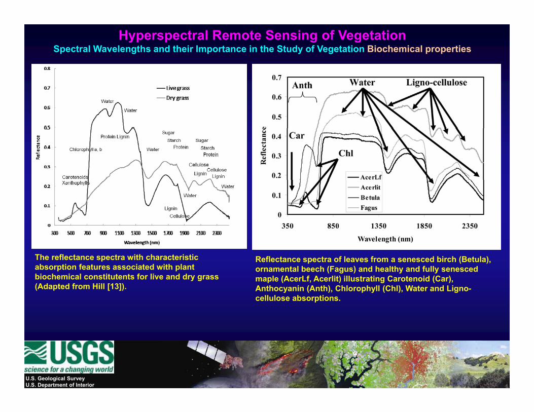
Hyperspectral Remote Sensing of Vegetation Spectral Wavelengths and their Importance in the Study of Vegetation Biochemical properties
Reflectance spectra of leaves from a senesced birch (Betula), ornamental beech (Fagus) and healthy and fully senesced maple (AcerLf, Acerlit) illustrating Carotenoid (Car),
The reflectance spectra with characteristic absorption features associated with plant biochemical constitutents for live and dry grass (Ad t d f Hill [13]) Anthocyanin (Anth), Chlorophyll (Chl), Water and Ligno-
cellulose absorptions.(Adapted from Hill [13]).
U.S. Geological SurveyU.S. Department of Interior
Definition of Hyperspectral Sensors (Imaging Spectrometry) inHyperspectral Sensors (Imaging Spectrometry) in
Study of Vegetation
U.S. Geological SurveyU.S. Department of Interior
Hyperspectral Remote Sensing of Vegetation Definition of Hyperspectral Data
A. consists of hundreds or thousands of narrow-wavebands (as narrow as 1; but generally less than 5 nm) along the electromagnetic spectrum; g p ;
B. it is important to have narrowbands that are contiguous for strict definition of hyperspectral data; and not so much the number of bands alone (Qi et al. in Chapter 3, Goetz and Shippert).
………….Hyperspectral Data is fast emerging to provide practical solutions in characterizing, quantifying, modeling, and mapping
t l t ti d i lt lnatural vegetation and agricultural crops.
30
40
50
e (p
erce
nt)
Y. sec. Forest
P. forest
Slash&Burn30
40
50
(per
cent
) Y. sec. Forest
P. forest
0
10
20
400 460 520 580 640 700 760 820 880 940 1000Wavelength (nm)
Ref
lect
ance
Raphia palm
Bamboo
P. Africana0
10
20
400 900 1400 1900 2400Wavelength (nm)
Ref
lect
ance
(
Slash&Burn
Raphia palm
Bamboo
P. Africana
U.S. Geological SurveyU.S. Department of Interior
Wavelength (nm)
The advantage of airborne, ground-based, and truck-mounted sensors are that they
Hyperspectral Remote Sensing of Vegetation Truck-mounted Hyperspectral sensors
enable relatively cloud free acquisitions that can be acquired on demand anywhere; over the years they have also allowed careful study of spectra in controlled environments to advance the genre.
Truck-mounted Hyperspectral Data Acquisition example
U.S. Geological SurveyU.S. Department of Interior
yp p q p
There are some twenty spaceborne hyperspectral
Hyperspectral Remote Sensing of Vegetation Spaceborne Hyperspectral Imaging Sensors: Some Characteristics
sensors
The advantages of spaceborne systems are their capability to acquire data: (a) continuously, (b) consistently, and (c) over the entire globe. A number y, ( ) gof system design challenges of hyperspectral data are discussed in Chapter 3 by Qi et al. Challenges include cloud cover and large data volumes.
Th 4 f h l b i iThe 4 near future hyperspectral spaceborne missions: 1. PRISMA (Italy’s ASI’s), 2. EnMAP (Germany’s DLR’s), and 3. HISUI (Japanese JAXA);4. HyspIRI (USA’s NASA).4. HyspIRI (USA s NASA). will all provide 30 m spatial resolution hyperspectralimages with a 30 km swath width, which may enable a provision of high temporal resolution, multi-angular hyperspectral observations over the same targets for the hyperspectral BRDF characterization of surfacethe hyperspectral BRDF characterization of surface.
The multi-angular hyperspectral observation capability may be one of next important steps in the field of hyperspectral remote sensing.
Existing hyperspectral spaceborne missions: 1. Hyperion (USA’s NASA), 2. PROBA (Europe’s ESA;’s), and
U.S. Geological SurveyU.S. Department of Interior
y g
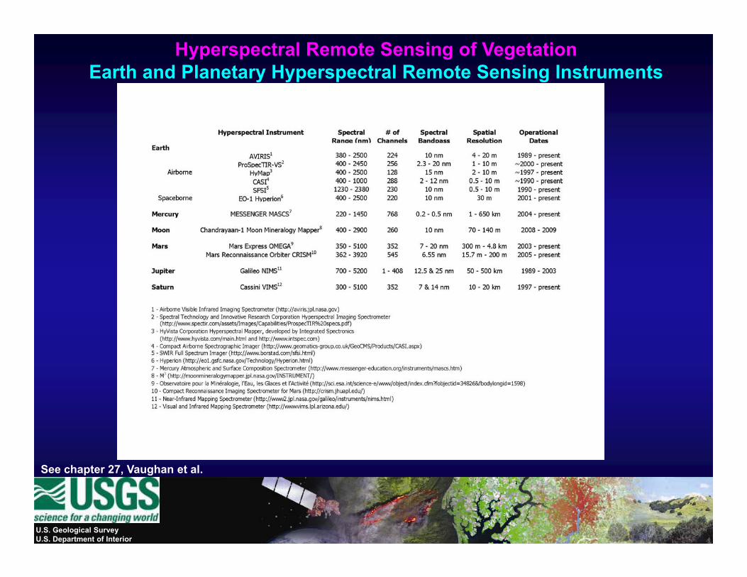
Hyperspectral Remote Sensing of Vegetation Earth and Planetary Hyperspectral Remote Sensing Instruments
See chapter 27 Vaughan et al
U.S. Geological SurveyU.S. Department of Interior
See chapter 27, Vaughan et al.
Satellite/Sensor spatial resolution spectral bands data points
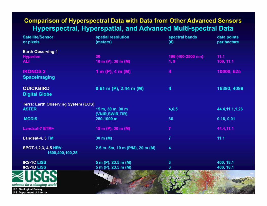
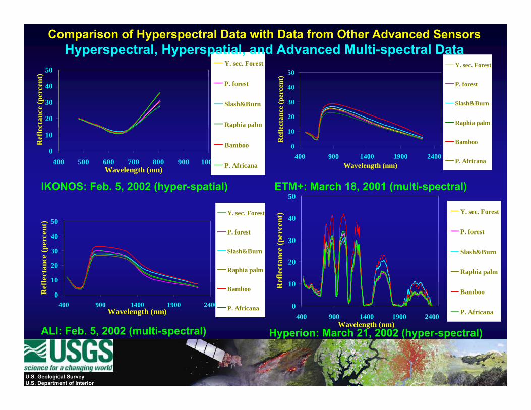
Comparison of Hyperspectral Data with Data from Other Advanced Sensors Hyperspectral, Hyperspatial, and Advanced Multi-spectral Data
Satellite/Sensor spatial resolution spectral bands data points or pixels (meters) (#) per hectare
Earth Observing-1Hyperion 30 196 (400-2500 nm) 11.1ALI 10 m (P), 30 m (M) 1, 9 100, 11.1
IKONOS 2 1 m (P), 4 m (M) 4 10000, 625SpaceImaging
QUICKBIRD 0.61 m (P), 2.44 m (M) 4 16393, 4098QU C 0 6 ( ), ( ) 6393, 098Digital Globe
Terra: Earth Observing System (EOS)ASTER 15 m, 30 m, 90 m 4,6,5 44.4,11.1,1.26
(VNIR,SWIR,TIR)( )MODIS 250-1000 m 36 0.16, 0.01
Landsat-7 ETM+ 15 m (P), 30 m (M) 7 44.4,11.1
Landsat-4, 5 TM 30 m (M) 7 11.1
SPOT-1,2,3, 4,5 HRV 2.5 m. 5m, 10 m (P/M), 20 m (M) 41600,400,100,25
IRS-1C LISS 5 m (P), 23.5 m (M) 3 400, 18.1IRS-1D LISS 5 m (P) 23 5 m (M) 3 400 18 1IRS 1D LISS 5 m (P), 23.5 m (M) 3 400, 18.1
U.S. Geological SurveyU.S. Department of Interior
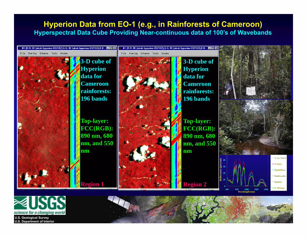
Hyperion Data from EO-1 (e.g., in Rainforests of Cameroon) Hyperspectral Data Cube Providing Near-continuous data of 100’s of Wavebands
3-D cube of Hyperion
3-D cube of Hyperion
data for Cameroon rainforests: 196 bands
data for Cameroon rainforests: 196 bands
Top-layer: FCC(RGB):
Top-layer: FCC(RGB):
890 nm, 680 nm, and 550 nm
890 nm, 680 nm, and 550 nm
40
50
cent
) Y. sec. Forest
P f t
Region 1 Region 2 0
10
20
30
400 900 1400 1900 2400Wavelength (nm)
Ref
lect
ance
(per
c P. forest
Slash&Burn
Raphia palm
Bamboo
P. Africana
U.S. Geological SurveyU.S. Department of Interior
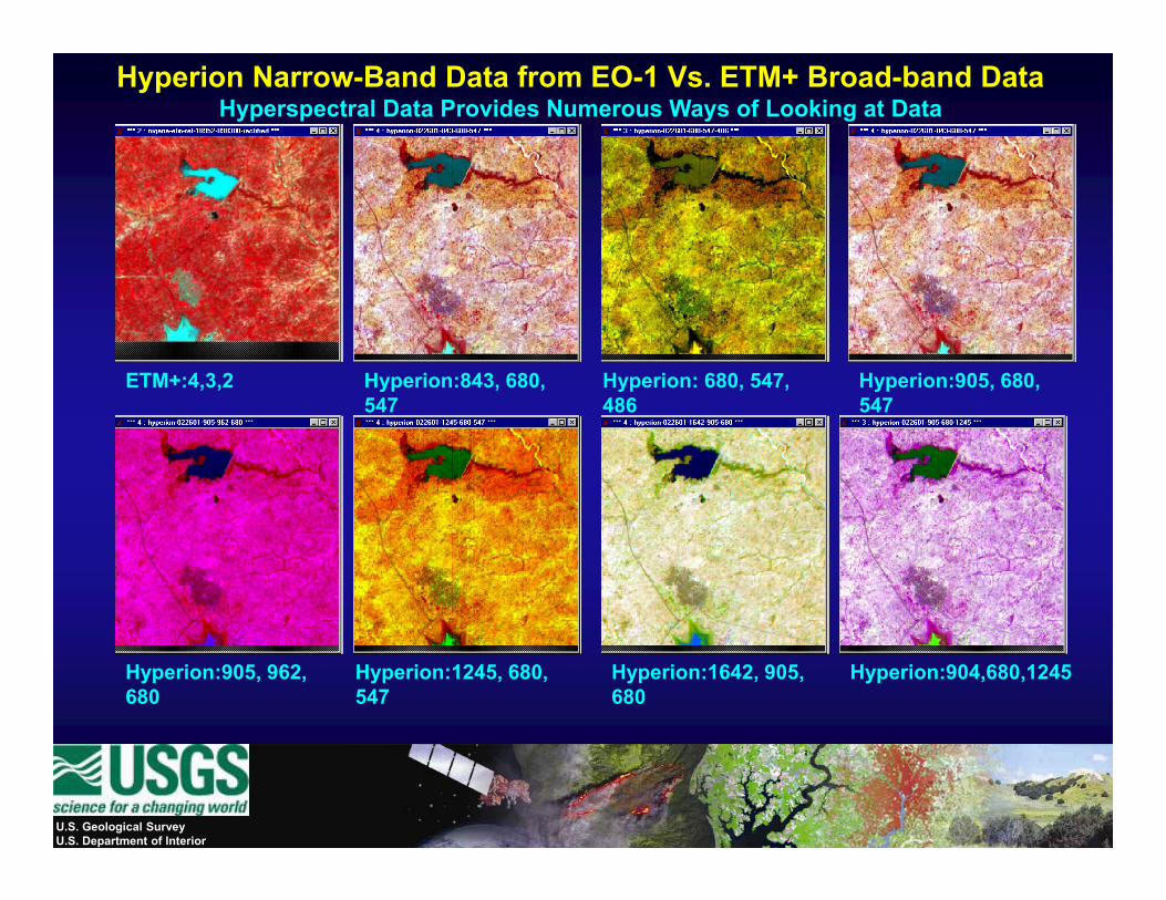
Hyperion Narrow-Band Data from EO-1 Vs. ETM+ Broad-band Data Hyperspectral Data Provides Numerous Ways of Looking at Data
Hyperion:843, 680, ETM+:4,3,2 Hyperion: 680, 547, Hyperion:905, 680, 547 486 547
Hyperion:905, 962, 680
Hyperion:1245, 680, 547
Hyperion:1642, 905, 680
Hyperion:904,680,1245
U.S. Geological SurveyU.S. Department of Interior
50)
Y. sec. Forest50
Y. sec. Forest
Comparison of Hyperspectral Data with Data from Other Advanced Sensors Hyperspectral, Hyperspatial, and Advanced Multi-spectral Data
20
30
40
ctan
ce (p
erce
nt)
P. forest
Slash&Burn
Raphia palm20
30
40
ecta
nce
(per
cent
)
P. forest
Slash&Burn
Raphia palm
0
10
400 500 600 700 800 900 1000Wavelength (nm)
Ref
le
p p
Bamboo
P. Africana
0
10
400 900 1400 1900 2400Wavelength (nm)
Ref
le
Bamboo
P. Africana
50
nt)
Y. sec. Forest
P f t
40
50
rcen
t) Y. sec. Forest
P forest
IKONOS: Feb. 5, 2002 (hyper-spatial) ETM+: March 18, 2001 (multi-spectral)
10
20
30
40
flect
ance
(per
ce P. forest
Slash&Burn
Raphia palm
10
20
30
efle
ctan
ce (p
er P. forest
Slash&Burn
Raphia palm
0400 900 1400 1900 2400
Wavelength (nm)
Ref Bamboo
P. Africana 0
10
400 900 1400 1900 2400Wavelength (nm)
RBamboo
P. Africana
ALI: Feb. 5, 2002 (multi-spectral) Hyperion: March 21 2002 (hyper-spectral)ALI: Feb. 5, 2002 (multi spectral) Hyperion: March 21, 2002 (hyper-spectral)
U.S. Geological SurveyU.S. Department of Interior

Hyperspectral Data Characteristics Spect al Wa elengths and thei Impo tance inSpectral Wavelengths and their Importance in
Vegetation Studies
U.S. Geological SurveyU.S. Department of Interior
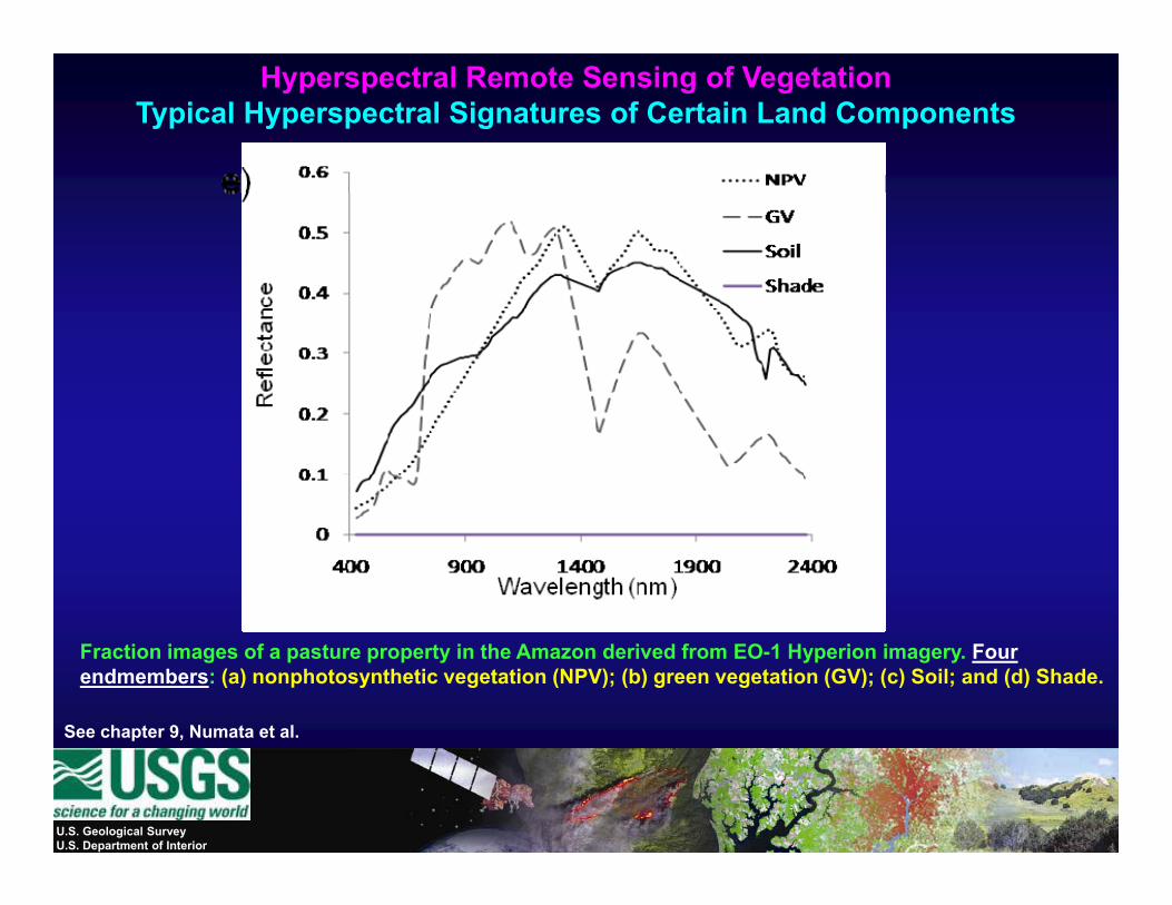
Hyperspectral Remote Sensing of Vegetation Typical Hyperspectral Signatures of Certain Land Components
See chapter 9, Numata et al.
Fraction images of a pasture property in the Amazon derived from EO-1 Hyperion imagery. Four endmembers: (a) nonphotosynthetic vegetation (NPV); (b) green vegetation (GV); (c) Soil; and (d) Shade.
U.S. Geological SurveyU.S. Department of Interior
p ,
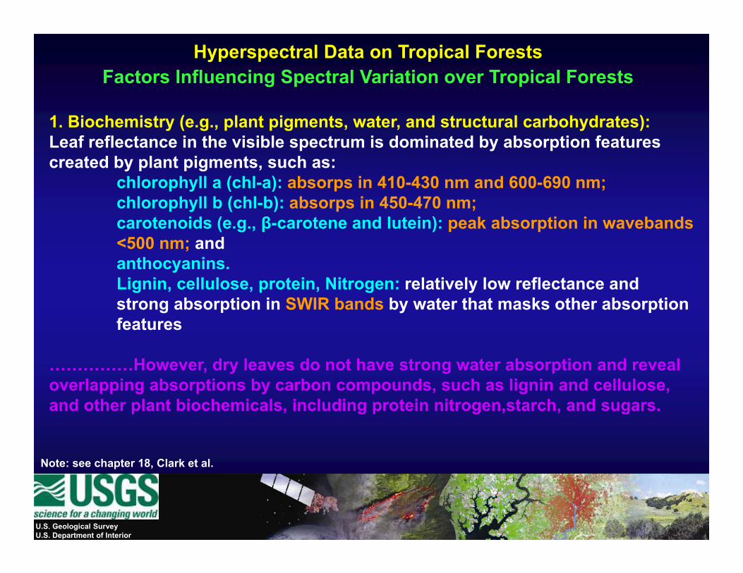
Hyperspectral Data on Tropical ForestsFactors Influencing Spectral Variation over Tropical Forests
1. Biochemistry (e.g., plant pigments, water, and structural carbohydrates): Leaf reflectance in the visible spectrum is dominated by absorption features created by plant pigments, such as:
hl h ll ( hl ) b i 410 430 d 600 690chlorophyll a (chl-a): absorps in 410-430 nm and 600-690 nm; chlorophyll b (chl-b): absorps in 450-470 nm;carotenoids (e.g., β-carotene and lutein): peak absorption in wavebands <500 nm; and;anthocyanins. Lignin, cellulose, protein, Nitrogen: relatively low reflectance and strong absorption in SWIR bands by water that masks other absorption featuresfeatures
……………However, dry leaves do not have strong water absorption and reveal overlapping absorptions by carbon compounds, such as lignin and cellulose,
Note: see chapter 18, Clark et al.
and other plant biochemicals, including protein nitrogen,starch, and sugars.
U.S. Geological SurveyU.S. Department of Interior
p ,
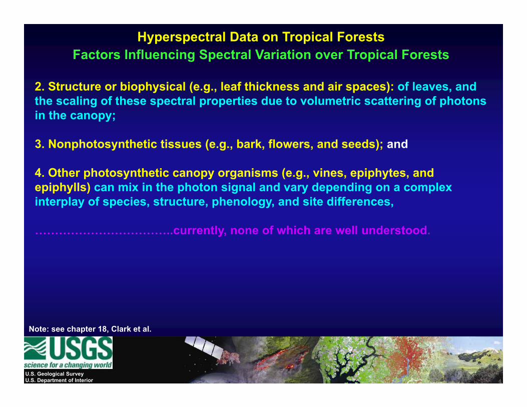
Hyperspectral Data on Tropical ForestsFactors Influencing Spectral Variation over Tropical Forests
2. Structure or biophysical (e.g., leaf thickness and air spaces): of leaves, and the scaling of these spectral properties due to volumetric scattering of photons in the canopy;
3. Nonphotosynthetic tissues (e.g., bark, flowers, and seeds); and
4. Other photosynthetic canopy organisms (e.g., vines, epiphytes, and p y py g ( g , , p p y ,epiphylls) can mix in the photon signal and vary depending on a complex interplay of species, structure, phenology, and site differences,
currently none of which are well understood……………………………..currently, none of which are well understood.
Note: see chapter 18, Clark et al.
U.S. Geological SurveyU.S. Department of Interior
p ,
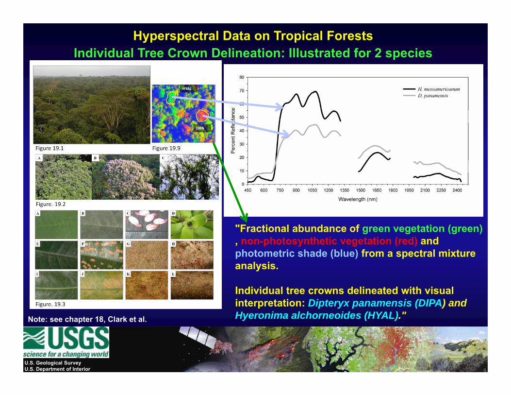
Hyperspectral Data on Tropical ForestsIndividual Tree Crown Delineation: Illustrated for 2 species
"Fractional abundance of green vegetation (green) , non-photosynthetic vegetation (red) and photometric shade (blue) from a spectral mixture analysis.
Note: see chapter 18, Clark et al.
Individual tree crowns delineated with visual interpretation: Dipteryx panamensis (DIPA) and Hyeronima alchorneoides (HYAL)."
U.S. Geological SurveyU.S. Department of Interior
p ,
African savannas d R i f t
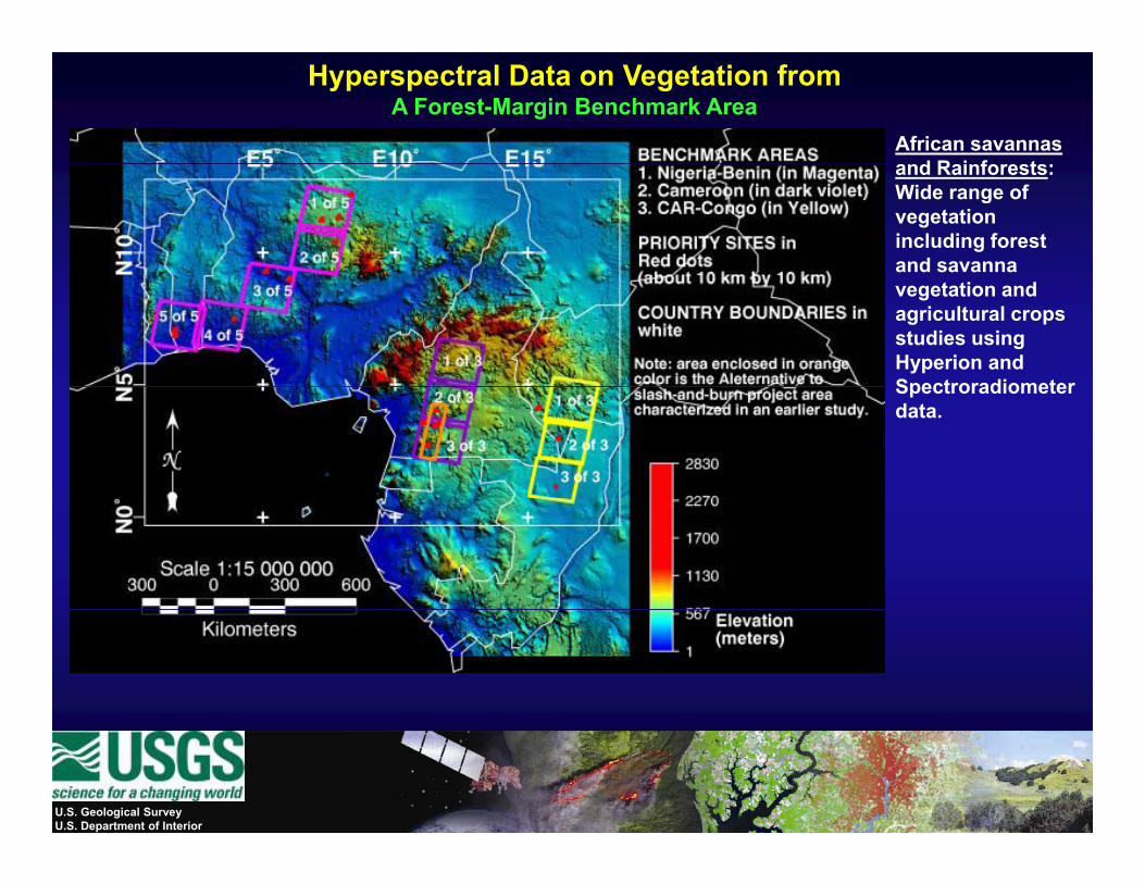
Hyperspectral Data on Vegetation from A Forest-Margin Benchmark Area
and Rainforests: Wide range of vegetation including forest and savanna vegetation and agricultural crops studies using Hyperion and SpectroradiometerSpectroradiometer data.
U.S. Geological SurveyU.S. Department of Interior
M fl t f Ch l d t d I t li d i
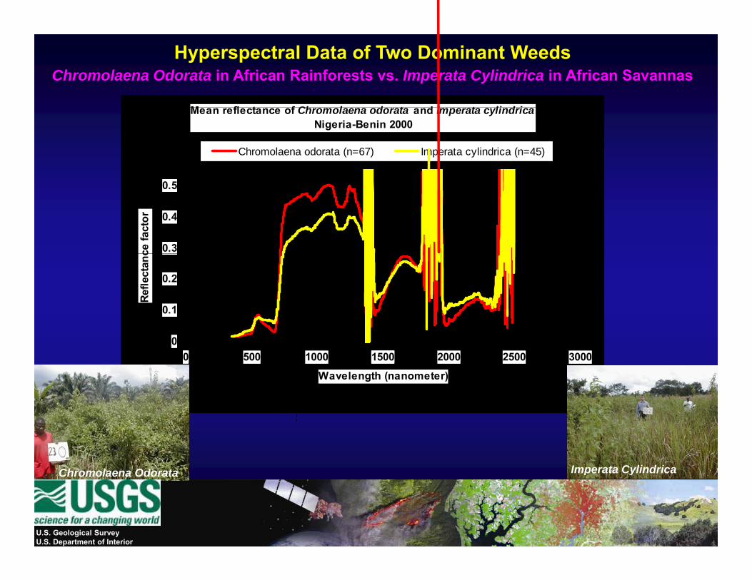
Hyperspectral Data of Two Dominant WeedsChromolaena Odorata in African Rainforests vs. Imperata Cylindrica in African Savannas
Mean reflectance of Chromolaena odorata and Imperata cylindricaNigeria-Benin 2000
Chromolaena odorata (n=67) Imperata cylindrica (n=45)
0.3
0.4
0.5
ce fa
ctor
0.1
0.2
Refle
ctan
c
00 500 1000 1500 2000 2500 3000
Wavelength (nanometer)
Chromolaena Odorata Imperata CylindricaChromolaena Odorata Imperata Cylindrica
U.S. Geological SurveyU.S. Department of Interior
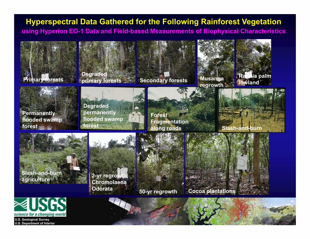
Hyperspectral Data Gathered for the Following Rainforest Vegetationusing Hyperion EO-1 Data and Field-based Measurements of Biophysical Characteristics
R hi lDegradedPrimary forests
D d d
Raphia palm lowland
Musanga regrowth
Secondary forestsDegraded primary forests
Slash-and-burn
Forest Fragmentation along roads
Degraded permanently flooded swamp forest
Permanently flooded swamp forest
Slash-and-burn agriculture
2-yr regrowth; Chromolaena Odorata 50-yr regrowth Cocoa plantations
U.S. Geological SurveyU.S. Department of Interior
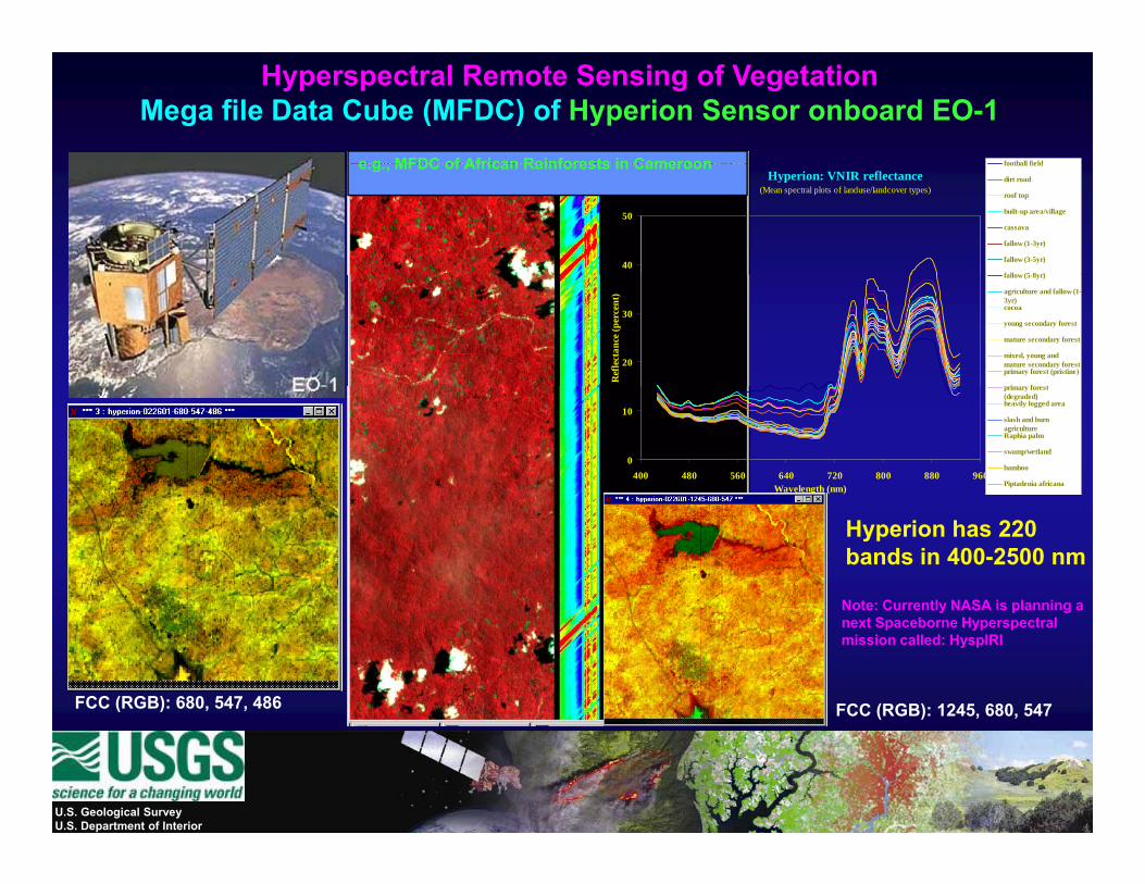
football field
Hyperspectral Remote Sensing of Vegetation Mega file Data Cube (MFDC) of Hyperion Sensor onboard EO-1
e g MFDC of African Rainforests in CameroonHyperion: VNIR reflectance
(Mean spectral plots of landuse/landcover types)
40
50
football field
dirt road
roof top
built-up area/village
cassava
fallow (1-3yr)
fallow (3-5yr)
fallow (5 8yr)
e.g., MFDC of African Rainforests in Cameroon
20
30
Ref
lect
ance
(per
cent
)
fallow (5-8yr)
agriculture and fallow (1-3yr)cocoa
young secondary forest
mature secondary forest
mixed, young andmature secondary forestprimary forest (pristine)
primar forest
0
10
400 480 560 640 720 800 880 960Wavelength (nm)
primary forest(degraded)heavily logged area
slash and burnagricultureRaphia palm
swamp/wetland
bamboo
Piptadenia africana
Hyperion has 220 bands in 400-2500 nm
Note: Currently NASA is planning a
FCC (RGB): 1245, 680, 547FCC (RGB): 680, 547, 486
Note: Currently NASA is planning a next Spaceborne Hyperspectral mission called: HyspIRI
U.S. Geological SurveyU.S. Department of Interior
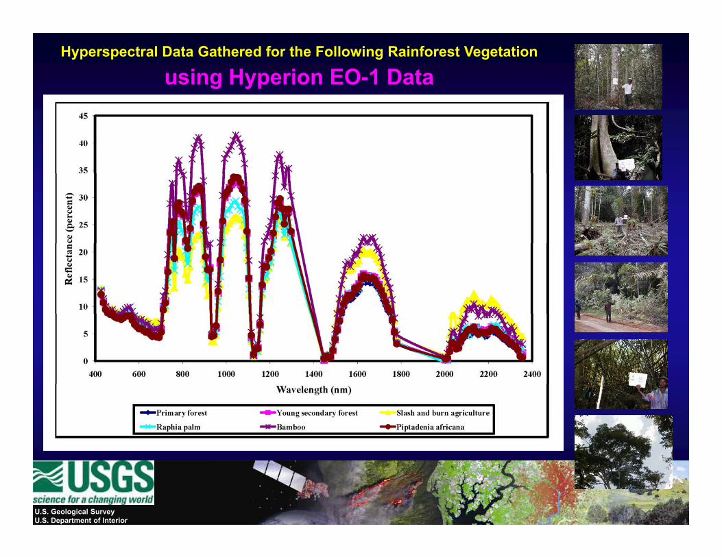
Hyperspectral Data Gathered for the Following Rainforest Vegetation
using Hyperion EO-1 Data
U.S. Geological SurveyU.S. Department of Interior
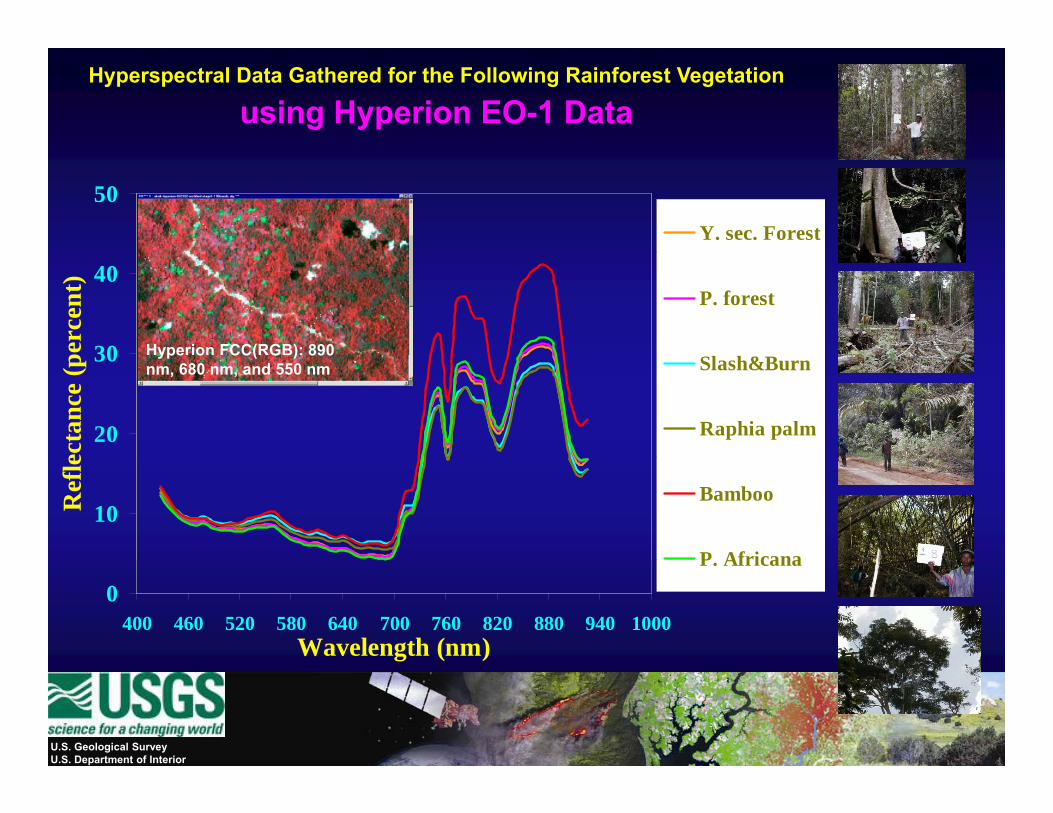
Hyperspectral Data Gathered for the Following Rainforest Vegetation
using Hyperion EO-1 Data
50Y. sec. Forest
30
40
perc
ent) P. forest
Hyperion FCC(RGB): 890
20
30
ecta
nce
(p Slash&Burn
Raphia palm
ype o CC( G ) 890nm, 680 nm, and 550 nm
10Ref
le
Bamboo
P Africana
0400 460 520 580 640 700 760 820 880 940 1000
Wavelength (nm)
P. Africana
U.S. Geological SurveyU.S. Department of Interior
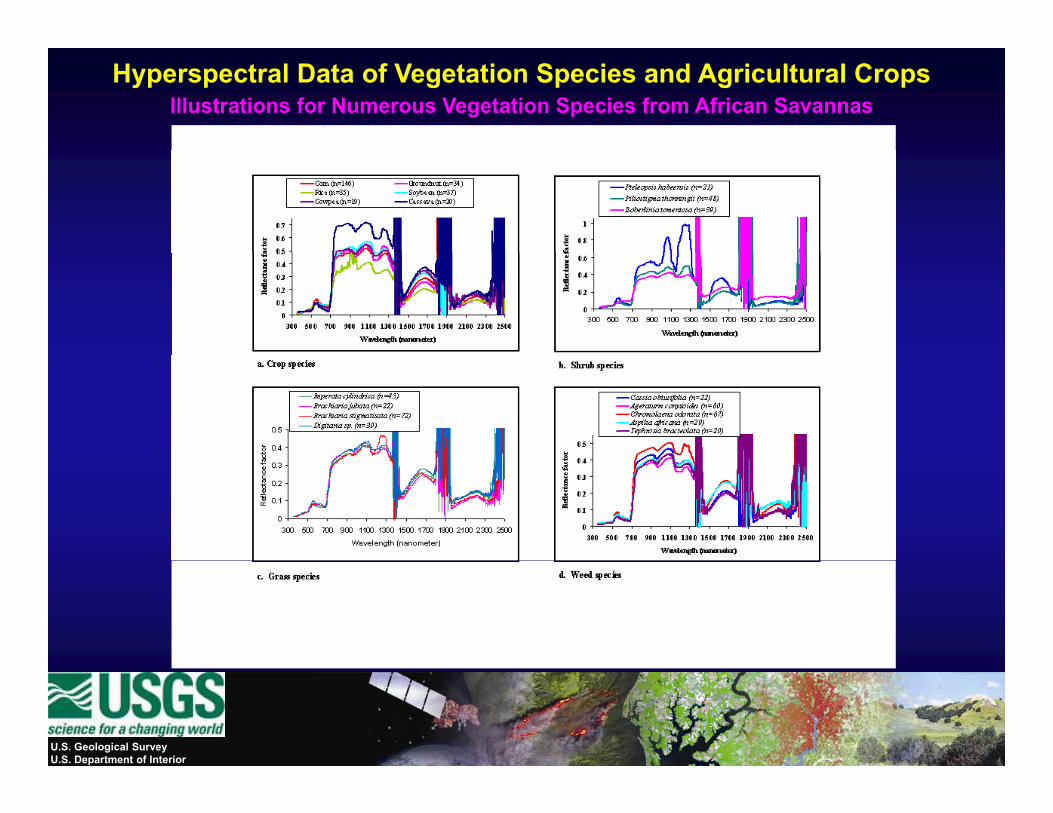
Hyperspectral Data of Vegetation Species and Agricultural CropsIllustrations for Numerous Vegetation Species from African Savannas
U.S. Geological SurveyU.S. Department of Interior
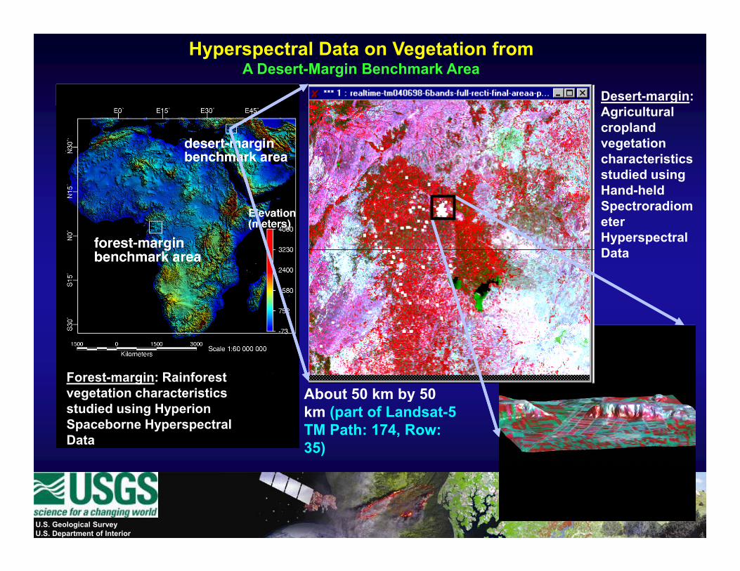
Hyperspectral Data on Vegetation from A Desert-Margin Benchmark Area
Desert-margin: Agricultural cropland vegetation characteristics studied usingstudied using Hand-held Spectroradiometer Hyperspectral D tData
About 50 km by 50Forest-margin: Rainforest vegetation characteristics About 50 km by 50
km (part of Landsat-5 TM Path: 174, Row: 35)
ICARDA research farms within
vegetation characteristics studied using Hyperion Spaceborne Hyperspectral Data
ICARDA research farms within the study area draped over 10-m DEM from Russian TK-350 Camera system
U.S. Geological SurveyU.S. Department of Interior
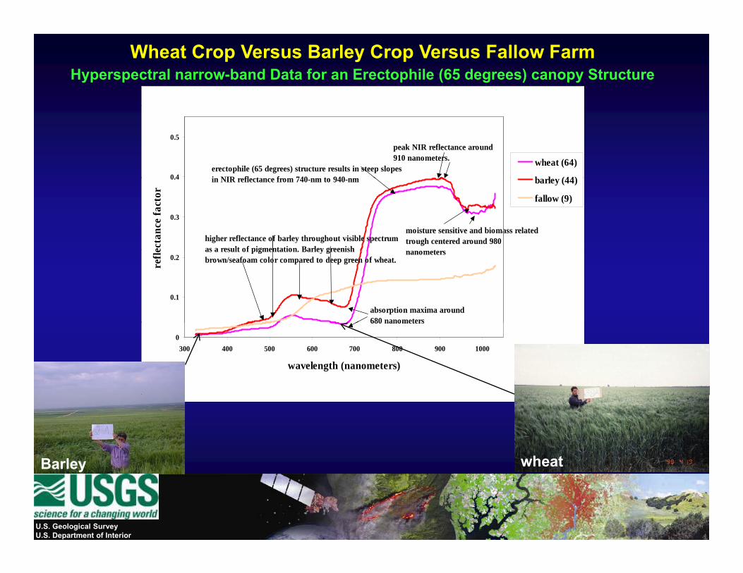
Wheat Crop Versus Barley Crop Versus Fallow FarmHyperspectral narrow-band Data for an Erectophile (65 degrees) canopy Structure
0 4
0.5
wheat (64)
b l (44)
peak NIR reflectance around 910 nanometers.
erectophile (65 degrees) structure results in steep slopes in NIR reflectance from 740 nm to 940 nm
0.3
0.4
ecta
nce
fact
or
barley (44)
fallow (9)
higher reflectance of barley throughout visible spectrum as a result of pigmentation Barley greenish
moisture sensitive and biomass related trough centered around 980
t
in NIR reflectance from 740-nm to 940-nm
0.1
0.2
refle
as a result of pigmentation. Barley greenish brown/seafoam color compared to deep green of wheat.
absorption maxima around680 nanometers
nanometers
0300 400 500 600 700 800 900 1000
wavelength (nanometers)
680 nanometers
wheatBarleyBarley
U.S. Geological SurveyU.S. Department of Interior
0.7 0.8
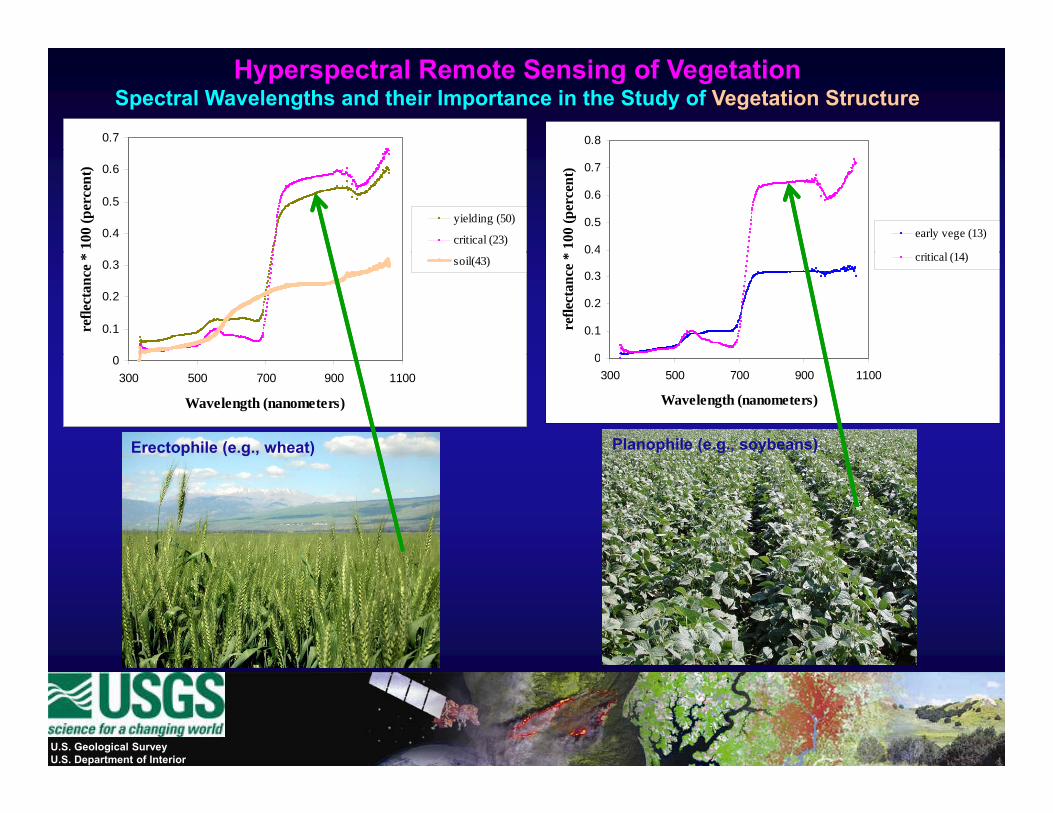
Hyperspectral Remote Sensing of Vegetation Spectral Wavelengths and their Importance in the Study of Vegetation Structure
0.4
0.5
0.6
100
(per
cent
)
yielding (50)
critical (23)0.4
0.5
0.6
0.7
100
(per
cent
)
early vege (13)
i i l (14)
0.1
0.2
0.3
refle
ctan
ce *
soil(43)
0
0.1
0.2
0.3
0.4
refle
ctan
ce * critical (14)
0300 500 700 900 1100
Wavelength (nanometers)
0300 500 700 900 1100
Wavelength (nanometers)
Erectophile (e.g., wheat) Planophile (e.g., soybeans)
U.S. Geological SurveyU.S. Department of Interior
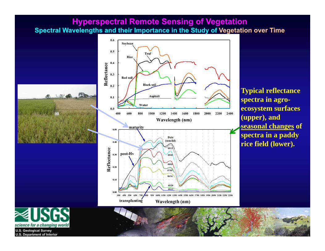
Hyperspectral Remote Sensing of Vegetation Spectral Wavelengths and their Importance in the Study of Vegetation over Time
Typical reflectance spectra in agro-ecosystem surfacesecosystem surfaces (upper), and seasonal changes of spectra in a paddy i fi ld (l )rice field (lower).
U.S. Geological SurveyU.S. Department of Interior

Hyperspectral Remote Sensing of Vegetation Spectral Wavelengths and their Importance in the Study of Vegetation Stress
See chapter 23
U.S. Geological SurveyU.S. Department of Interior
See chapter 23
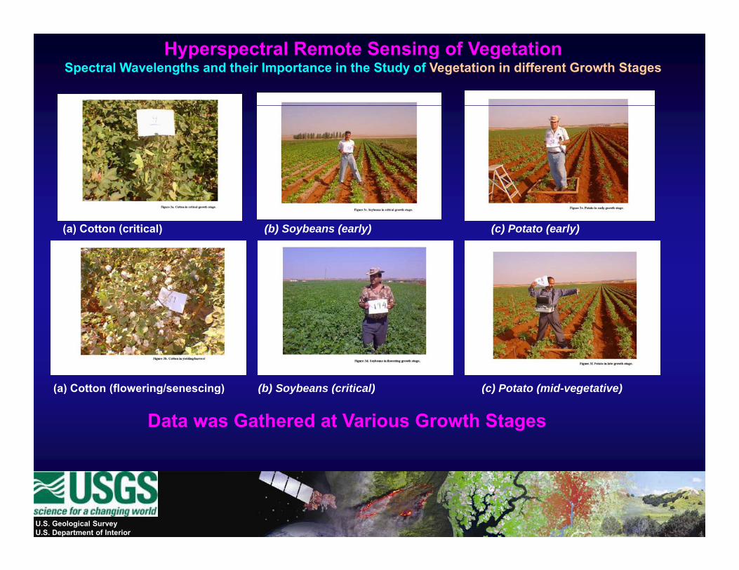
Hyperspectral Remote Sensing of Vegetation Spectral Wavelengths and their Importance in the Study of Vegetation in different Growth Stages
(a) Cotton (critical) (b) Soybeans (early) (c) Potato (early)
(a) Cotton (flowering/senescing) (b) Soybeans (critical) (c) Potato (mid-vegetative)( ) ( g g) ( ) y ( ) ( ) ( g )
Data was Gathered at Various Growth Stages
U.S. Geological SurveyU.S. Department of Interior
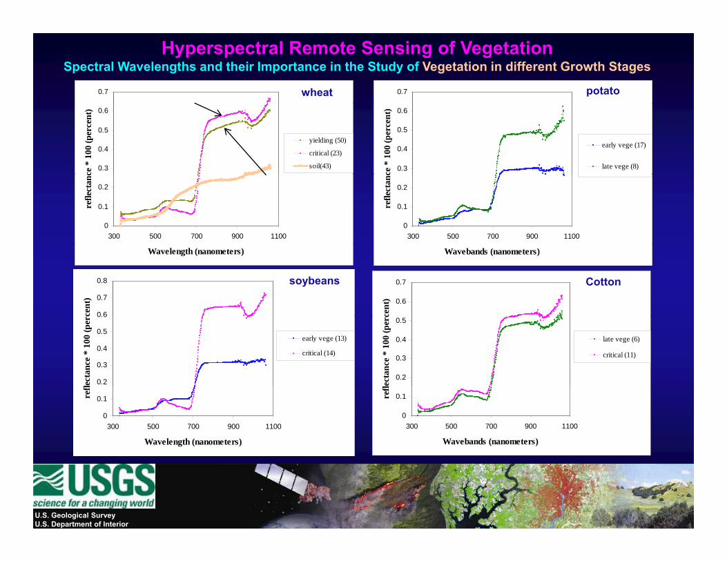
0.7 0.7
Hyperspectral Remote Sensing of Vegetation Spectral Wavelengths and their Importance in the Study of Vegetation in different Growth Stages
wheat potato
0.3
0.4
0.5
0.6
ce *
100
(per
cent
)
yielding (50)
critical (23)
soil(43) 0.3
0.4
0.5
0.6
ce *
100
(per
cent
)
early vege (17)
late vege (8)
0
0.1
0.2
300 500 700 900 1100
refle
ctan
c
0
0.1
0.2
300 500 700 900 1100
refle
ctan
c
Wavelength (nanometers) Wavebands (nanometers)
0 6
0.7
0.8
cent
) 0.6
0.7
cent
)
Cottonsoybeans
0.2
0.3
0.4
0.5
0.6
lect
ance
* 1
00 (p
erc
early vege (13)
critical (14)
0.2
0.3
0.4
0.5
lect
ance
* 1
00 (p
erc
late vege (6)
critical (11)
0
0.1
300 500 700 900 1100
Wavelength (nanometers)
refl
0
0.1
300 500 700 900 1100
Wavebands (nanometers)
refl
U.S. Geological SurveyU.S. Department of Interior
Hughes Phenomenon (or Curse of High Dimensionality of Data) and(or Curse of High Dimensionality of Data) and
overcoming data redundancy through Data Mining
U.S. Geological SurveyU.S. Department of Interior
Hyperspectral Data (Imaging Spectroscopy data) Not a Panacea!
For example, hyperspectral systems collect large volumes of data in a short time. Issues include:
data storage volume;data storage rate;downlink or transmission bandwidth;computing bottle neck in data analysis; andnew algorithms for data utilization (e g atmosphericnew algorithms for data utilization (e.g., atmospheric correction more complicated).
U.S. Geological SurveyU.S. Department of Interior
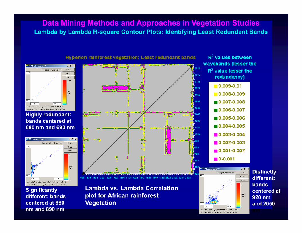
Data Mining Methods and Approaches in Vegetation StudiesLambda by Lambda R-square Contour Plots: Identifying Least Redundant Bands
Highly redundant: bands centered at 680 nm and 690 nm
Significantly
Distinctly different: bands centered atLambda vs. Lambda CorrelationSignificantly
different: bands centered at 680 nm and 890 nm
centered at 920 nm and 2050 nm
Lambda vs. Lambda Correlation plot for African rainforest Vegetation
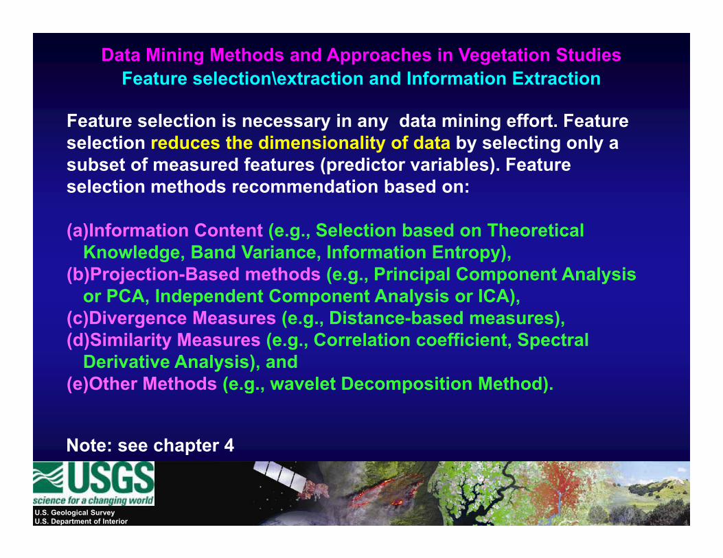
Data Mining Methods and Approaches in Vegetation Studies Feature selection\extraction and Information Extraction
Feature selection is necessary in any data mining effort. Feature selection reduces the dimensionality of data by selecting only a subset of measured features (predictor variables). Feature (p )selection methods recommendation based on:
(a)Information Content (e.g., Selection based on Theoretical Knowledge, Band Variance, Information Entropy),
(b)Projection-Based methods (e.g., Principal Component Analysis or PCA, Independent Component Analysis or ICA),
( )Di M ( Di t b d )(c)Divergence Measures (e.g., Distance-based measures), (d)Similarity Measures (e.g., Correlation coefficient, Spectral
Derivative Analysis), and (e)Other Methods (e g wavelet Decomposition Method)(e)Other Methods (e.g., wavelet Decomposition Method).
Note: see chapter 4
U.S. Geological SurveyU.S. Department of Interior
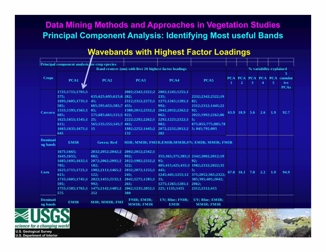
Data Mining Methods and Approaches in Vegetation Studies Principal Component Analysis: Identifying Most useful Bands
Principal component analysis for crop species
PCA PCA PCA PCA PCA5
cumulatCrops
% variability explainedBand centers (nm) with first 20 highest factor loadings
Wavebands with Highest Factor Loadings
PCA1 PCA2 PCA3 PCA4 PCA5 PCA1
PCA2
PCA3
PCA4
PCA5
cumulative
PCAs1725;1715;1705;1575; 1695;1605;1735;1585; 1555;1595;1565;1
635;625;695;615;645; 605;595;655;585;705;
2002;2342;2322;2282; 2312;2312;2272;1455; 1380;2012;2332;2
2002;1245;1255;1235; 1275;1265;1285;1992; 2042;2032;2262;2
2332;2342;2322;1982; 2312;2312;1445;2292;
Crops
Cassava 1555;1595;1565;1685; 1625;1655;1545;1615; 1665;1635;1675;1645
05; 575;685;665;515;525; 565;535;555;545;715
1380;2012;2332;2022; 2222;2292;2262;1465; 1982;2252;1445;2132
2042;2032;2262;2062; 2292;1225;2322;1982; 2072;2232;2012;2282
92; 2022;1992;2262;865; 875;855;775;885;785; 845;795;805
63.9 18.9 5.6 2.6 1.9 92.7
DominatiEMIR Green; Red EMIR; MMIR; FMIRR;EMIR;MMIR;FMR; EMIR; MMIR; FMIRng bands EMIR Green; Red EMIR; MMIR; FMIRR;EMIR;MMIR;FMR; EMIR; MMIR; FMIR
Corn
1675;1665; 1645;1655; 1685;1695;1635;1705; 1625;1715;1725;1615
2032;2052;2042;2082; 2072;2062;2092;2102; 1982;2112;1465;2122
2002;2012;2342;1992; 2022;1982;2332;2322; 2032;2072;1255;1245
355;365;375;385;395; 405;415;425;435;1445; 1245 445 1255 12
2342;2002;2012;1992; 1982;2332;2022;355; 375 2052 365 2322
67.0 16.1 7.8 2.2 1.9 94.9615; 1735;1605;1745;1595; 1755;1585;1765;1575
122; 2022;1455;2132;1992; 1475;2142;1485;2252
245; 2042;1275;1285;1265; 2062;1235;2052;1380
1245;445;1255;1235; 1275;1265;1285;1225; 1135;1455
375;2052;365;2322; 385;395;405;2042; 2062; 2312;2312;415
Dominating bands EMIR EMIR; MMIR; FMIR
FNIR; EMIR; MMIR; FMIR
UV; Blue; FNIR; EMIR
UV; Blue; EMIR; MMIR; FMIRg ; ;
U.S. Geological SurveyU.S. Department of Interior

Methods of Modeling Vegetation Characteristics usingModeling Vegetation Characteristics using
Hyperspectral Vegetation Indices (HVIs)
U.S. Geological SurveyU.S. Department of Interior
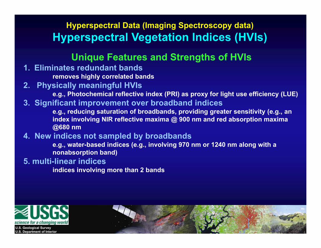
Hyperspectral Data (Imaging Spectroscopy data) Hyperspectral Vegetation Indices (HVIs)
Unique Features and Strengths of HVIs1. Eliminates redundant bands
removes highly correlated bandsremoves highly correlated bands2. Physically meaningful HVIs
e.g., Photochemical reflective index (PRI) as proxy for light use efficiency (LUE)3. Significant improvement over broadband indices
e.g., reducing saturation of broadbands, providing greater sensitivity (e.g., an index involving NIR reflective maxima @ 900 nm and red absorption maxima @680 nm
4. New indices not sampled by broadbandsp ye.g., water-based indices (e.g., involving 970 nm or 1240 nm along with a nonabsorption band)
5. multi-linear indicesindices involving more than 2 bandsindices involving more than 2 bands
U.S. Geological SurveyU.S. Department of Interior
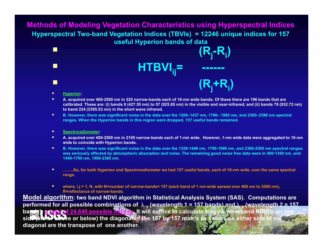
Methods of Modeling Vegetation Characteristics using Hyperspectral IndicesHyperspectral Two-band Vegetation Indices (TBVIs) = 12246 unique indices for 157
useful Hyperion bands of data(Rj-Ri)
HTBVIij= ------(Rj+Ri)
Hyperion: A. acquired over 400-2500 nm in 220 narrow-bands each of 10-nm wide bands. Of these there are 196 bands that are calibrated. These are: (i) bands 8 (427.55 nm) to 57 (925.85 nm) in the visible and near-infrared; and (ii) bands 79 (932.72 nm)to band 224 (2395 53 nm) in the short wave infraredto band 224 (2395.53 nm) in the short wave infrared. B. However, there was significant noise in the data over the 1206–1437 nm, 1790– 1992 nm, and 2365–2396 nm spectral ranges. When the Hyperion bands in this region were dropped, 157 useful bands remained.
Spectroradiometer: A. acquired over 400-2500 nm in 2100 narrow-bands each of 1-nm wide. However, 1-nm wide data were aggregated to 10-nm wide to coincide with Hyperion bands.B. However, there was significant noise in the data over the 1350-1440 nm, 1790-1990 nm, and 2360-2500 nm spectral ranges. was seriously affected by atmospheric absorption and noise. The remaining good noise free data were in 400-1350 nm, and 1440-1790 nm, 1990-2360 nm.
……..So, for both Hyperion and Spectroradiometer we had 157 useful bands, each of 10-nm wide, over the same spectral , yp p , , prange.
where, i,j = 1, N, with N=number of narrow-bands= 157 (each band of 1 nm-wide spread over 400 nm to 2500 nm), R=reflectance of narrow-bands.
Model algorithm: two band NDVI algorithm in Statistical Analysis System (SAS). Computations are f d f ll ibl bi ti f λ ( l th 1 157 b d ) d λ ( l th 2 157performed for all possible combinations of λ 1 (wavelength 1 = 157 bands) and λ 2 (wavelength 2 = 157
bands)- a total of 24,649 possible indices. It will suffice to calculate Narrow-waveband NDVI's on one side (either above or below) the diagonal of the 157 by 157 matrix as values on either side of the diagonal are the transpose of one another.
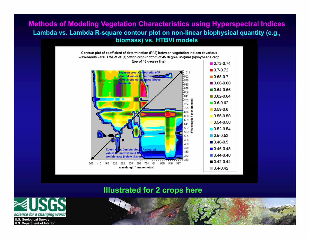
Methods of Modeling Vegetation Characteristics using Hyperspectral IndicesLambda vs. Lambda R-square contour plot on non-linear biophysical quantity (e.g.,
biomass) vs. HTBVI models
Illustrated for 2 crops here
U.S. Geological SurveyU.S. Department of Interior
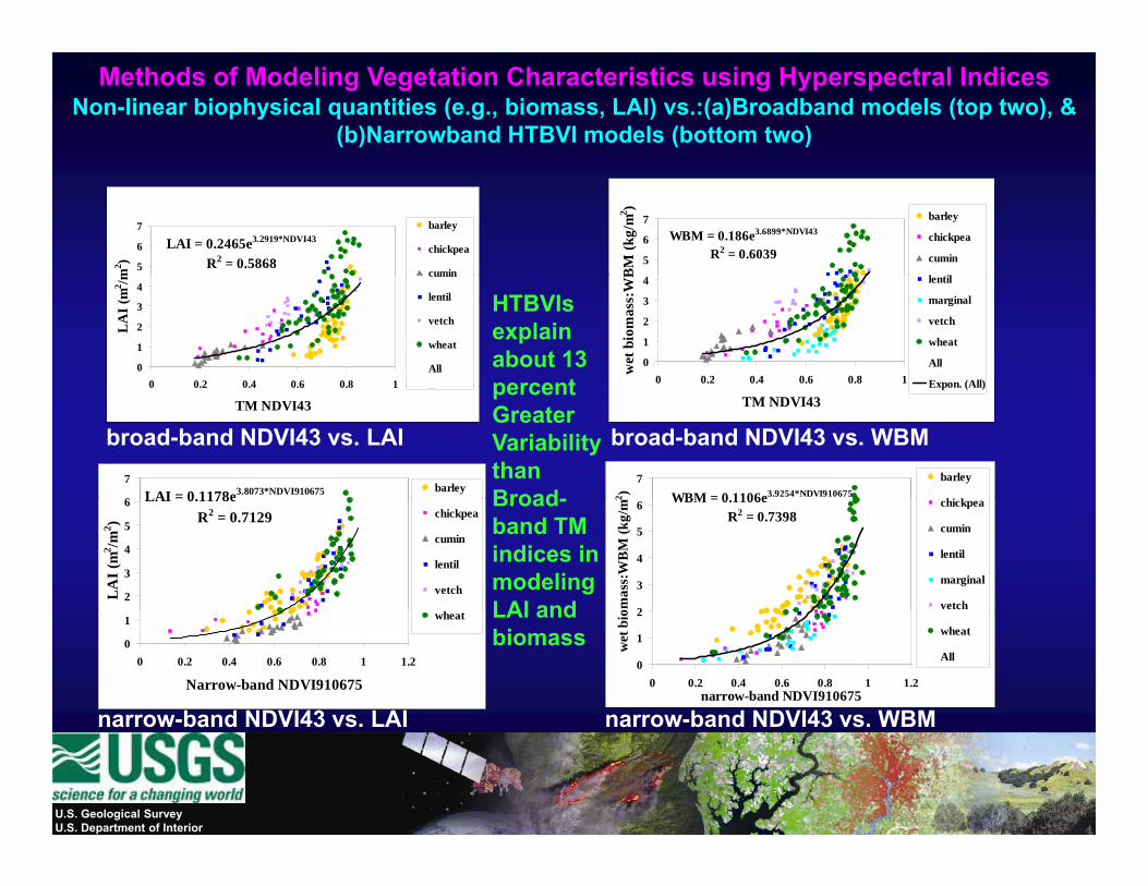
Methods of Modeling Vegetation Characteristics using Hyperspectral IndicesNon-linear biophysical quantities (e.g., biomass, LAI) vs.:(a)Broadband models (top two), &
(b)Narrowband HTBVI models (bottom two)
LAI = 0.2465e3.2919*NDVI43
R2 = 0.58685
6
7
m2 )
barley
chickpea
cumin
WBM = 0.186e3.6899*NDVI43
R2 = 0.60395
6
7
BM
(kg/
m2 )
barley
chickpea
cumin
l il
0
1
2
3
4
0 0.2 0.4 0.6 0.8 1
LA
I (m
2 /m cumin
lentil
vetch
wheat
All 0
1
2
3
4
0 0.2 0.4 0.6 0.8 1
wet
bio
mas
s:W
B lentil
marginal
vetch
wheat
All
Expon. (All)
HTBVIs explain about 13 percent0 0.2 0.4 0.6 0.8 1
TM NDVI43 E
TM NDVI43 Expon. (All)
LAI = 0.1178e3.8073*NDVI9106756
7barley
WBM = 0 1106e3.9254*NDVI9106757
2 )
barley
hi k
broad-band NDVI43 vs. LAI broad-band NDVI43 vs. WBM
percent Greater Variability than Broad-LAI 0.1178e
R2 = 0.7129
2
3
4
5
6
LA
I (m
2 /m2 ) chickpea
cumin
lentil
vetch
WBM = 0.1106eR2 = 0.7398
2
3
4
5
6
omas
s:W
BM
(kg/
m2 chickpea
cumin
lentil
marginal
vetch
Broad-band TM indices in modeling LAI and
0
1
0 0.2 0.4 0.6 0.8 1 1.2
Narrow-band NDVI910675
wheat
0
1
2
0 0.2 0.4 0.6 0.8 1 1.2narrow-band NDVI910675
wet
bio
wheat
All
narrow-band NDVI43 vs LAI narrow-band NDVI43 vs WBM
LAI and biomass
narrow band NDVI43 vs. LAI narrow band NDVI43 vs. WBM
U.S. Geological SurveyU.S. Department of Interior
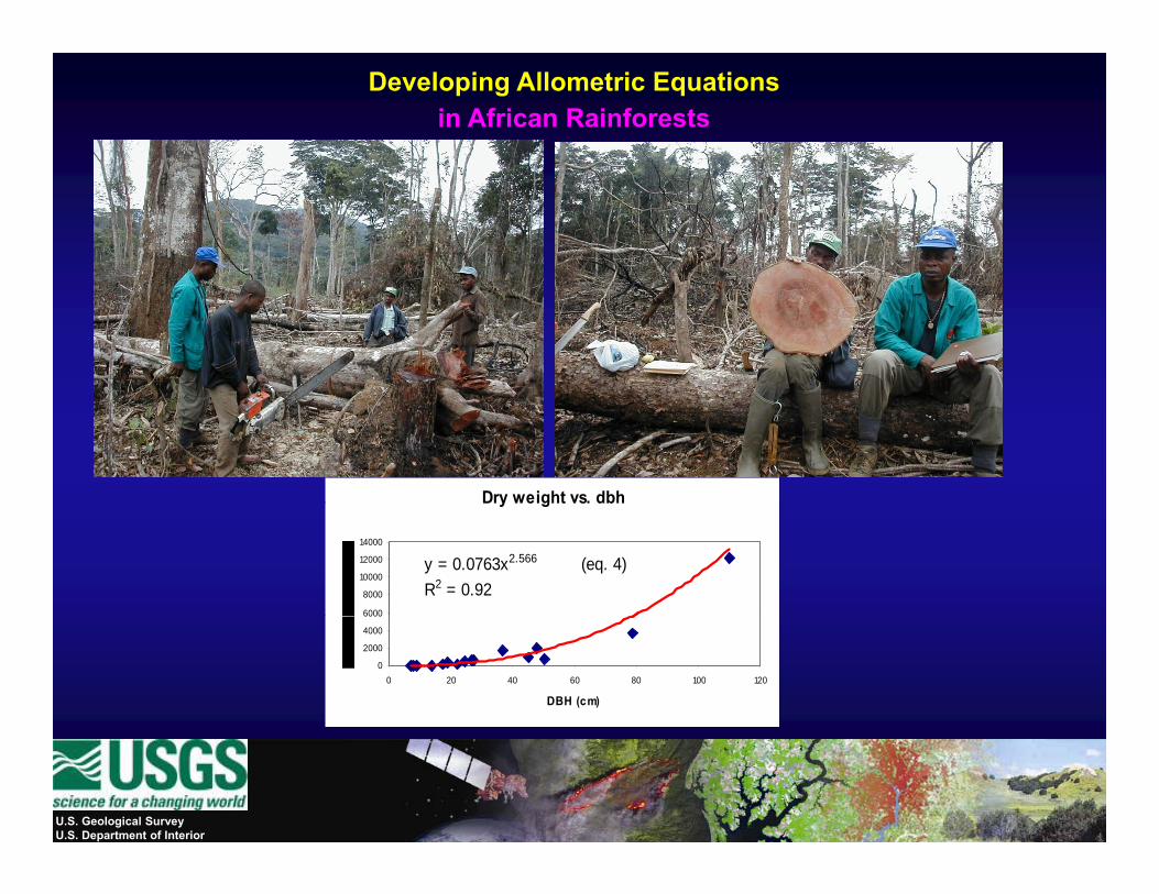
Developing Allometric Equations in African Rainforests
Dry weight vs. dbhy g
y = 0.0763x2.566 (eq. 4)R2 = 0.92
6000
8000
10000
12000
14000
0
2000
4000
6000
0 20 40 60 80 100 120
DBH (cm)
U.S. Geological SurveyU.S. Department of Interior

Methods of Modeling Vegetation Characteristics using Hyperspectral IndicesLambda vs. Lambda R-square contour plot on non-linear biophysical quantity (e.g.,
biomass) vs. HTBVI models
Waveband combinations with greatest R2 values Greater are ranked…….bandwidths can also be
<ths can also be determined.
U.S. Geological SurveyU.S. Department of Interior
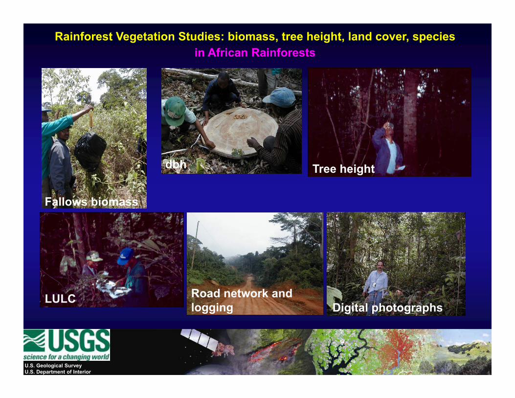
Rainforest Vegetation Studies: biomass, tree height, land cover, species in African Rainforests
Tree heightdbh
Fallows biomass
g
Road network and logging
LULCDigital photographs
U.S. Geological SurveyU.S. Department of Interior
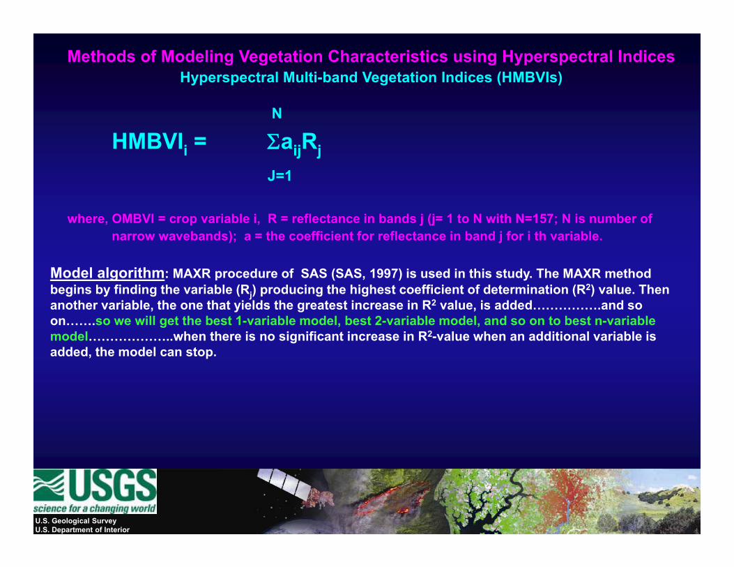
Methods of Modeling Vegetation Characteristics using Hyperspectral IndicesHyperspectral Multi-band Vegetation Indices (HMBVIs)
N
HMBVIi = ΣaijRjJ=1J=1
where, OMBVI = crop variable i, R = reflectance in bands j (j= 1 to N with N=157; N is number of narrow wavebands); a = the coefficient for reflectance in band j for i th variable.
Model algorithm: MAXR procedure of SAS (SAS, 1997) is used in this study. The MAXR method begins by finding the variable (Rj) producing the highest coefficient of determination (R2) value. Then another variable, the one that yields the greatest increase in R2 value, is added…………….and so on so we will get the best 1 variable model best 2 variable model and so on to best n variableon…….so we will get the best 1-variable model, best 2-variable model, and so on to best n-variable model………………..when there is no significant increase in R2-value when an additional variable is added, the model can stop.
U.S. Geological SurveyU.S. Department of Interior
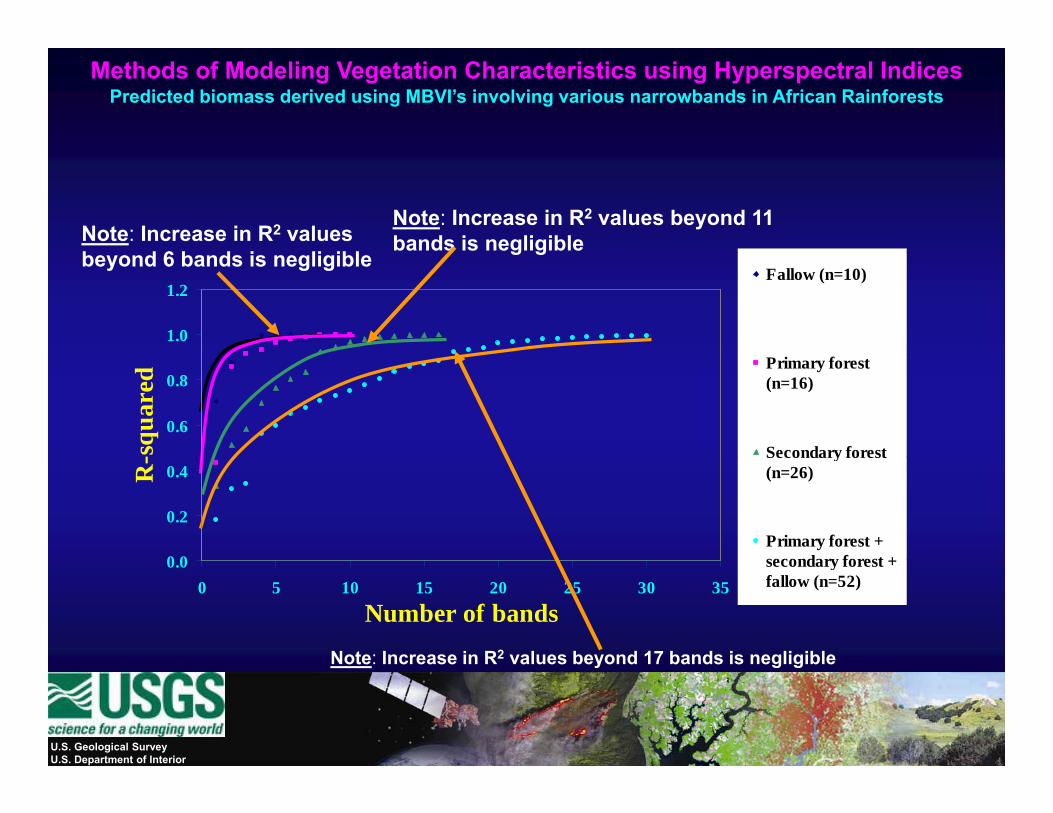
Methods of Modeling Vegetation Characteristics using Hyperspectral IndicesPredicted biomass derived using MBVI’s involving various narrowbands in African Rainforests
Note: Increase in R2 values beyond 11 bands is negligibleNote: Increase in R2 values
b d 6 b d i li ibl
1.0
1.2Fallow (n=10)
g gbeyond 6 bands is negligible
0.6
0.8
-squ
ared
Primary forest(n=16)
Secondary forest
0 0
0.2
0.4R- Seco d y o es
(n=26)
Primary forest +secondary forest +0.0
0 5 10 15 20 25 30 35
Number of bands
secondary forest +fallow (n=52)
Note: Increase in R2 values beyond 17 bands is negligibleNote: Increase in R values beyond 17 bands is negligible
U.S. Geological SurveyU.S. Department of Interior
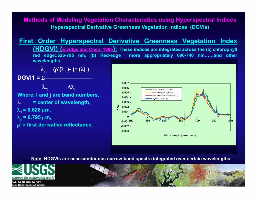
Methods of Modeling Vegetation Characteristics using Hyperspectral IndicesHyperspectral Derivative Greenness Vegetation Indices (DGVIs)
First Order Hyperspectral Derivative Greenness Vegetation Index(HDGVI) (Elvidge and Chen, 1995): These indices are integrated across the (a) chlorophyllred edge:.626-795 nm, (b) Red-edge more appropriately 690-740 nm……and otherwavelengthswavelengths.
λn (ρ′(λi )- (ρ′(λj )DGVI1 = Σ⎯⎯⎯⎯⎯⎯⎯⎯
λ Δλλ1 ΔλIWhere, I and j are band numbers,λ = center of wavelength,λ1 = 0.626 μm,λ1 0 6 6 μ ,λn = 0.795 μm,ρ′ = first derivative reflectance.
Note: HDGVIs are near-continuous narrow-band spectra integrated over certain wavelengths
U.S. Geological SurveyU.S. Department of Interior
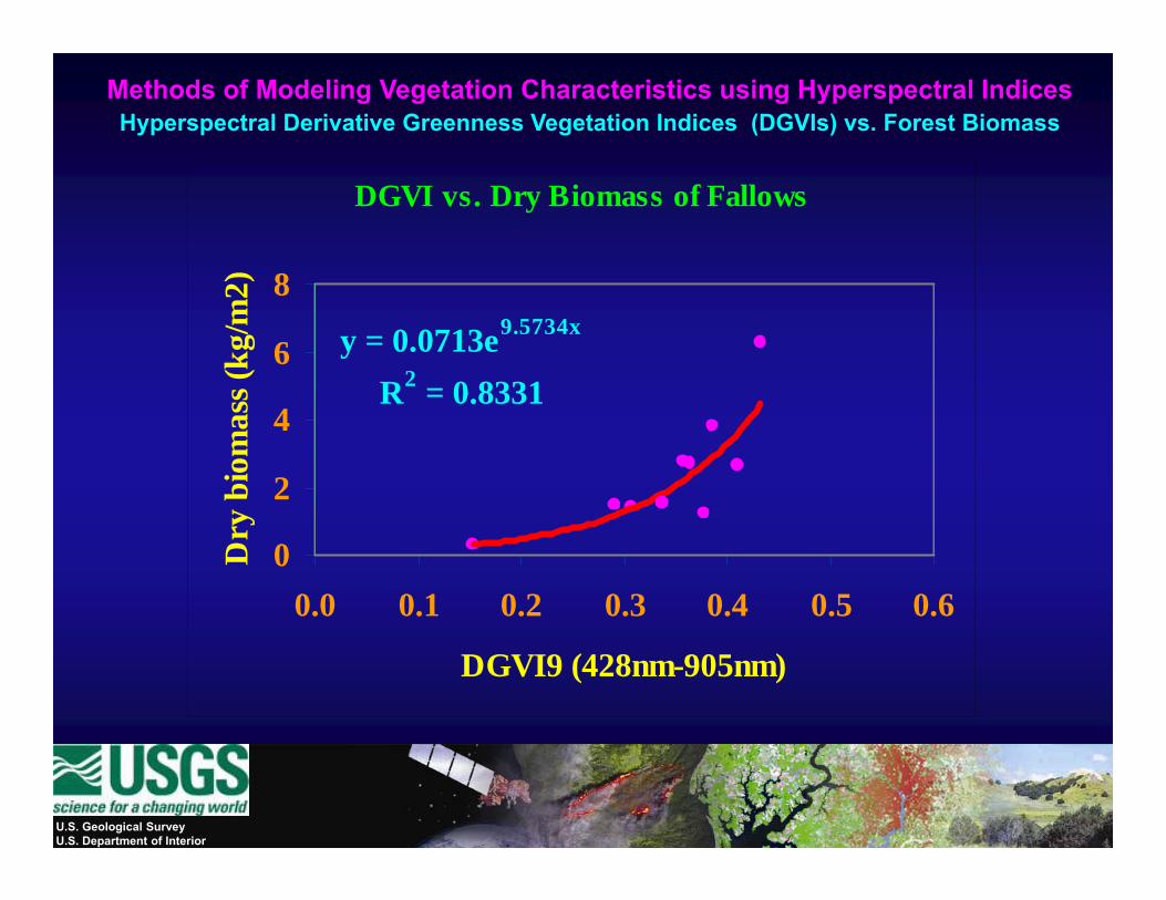
Methods of Modeling Vegetation Characteristics using Hyperspectral IndicesHyperspectral Derivative Greenness Vegetation Indices (DGVIs) vs. Forest Biomass
DGVI vs. Dry Biomass of Fallows
8)
y = 0.0713e9.5734x
R2 = 0 83316
8s (
kg/m
2)
R = 0.8331
2
4
biom
ass
00.0 0.1 0.2 0.3 0.4 0.5 0.6
Dry
DGVI9 (428nm-905nm)
U.S. Geological SurveyU.S. Department of Interior
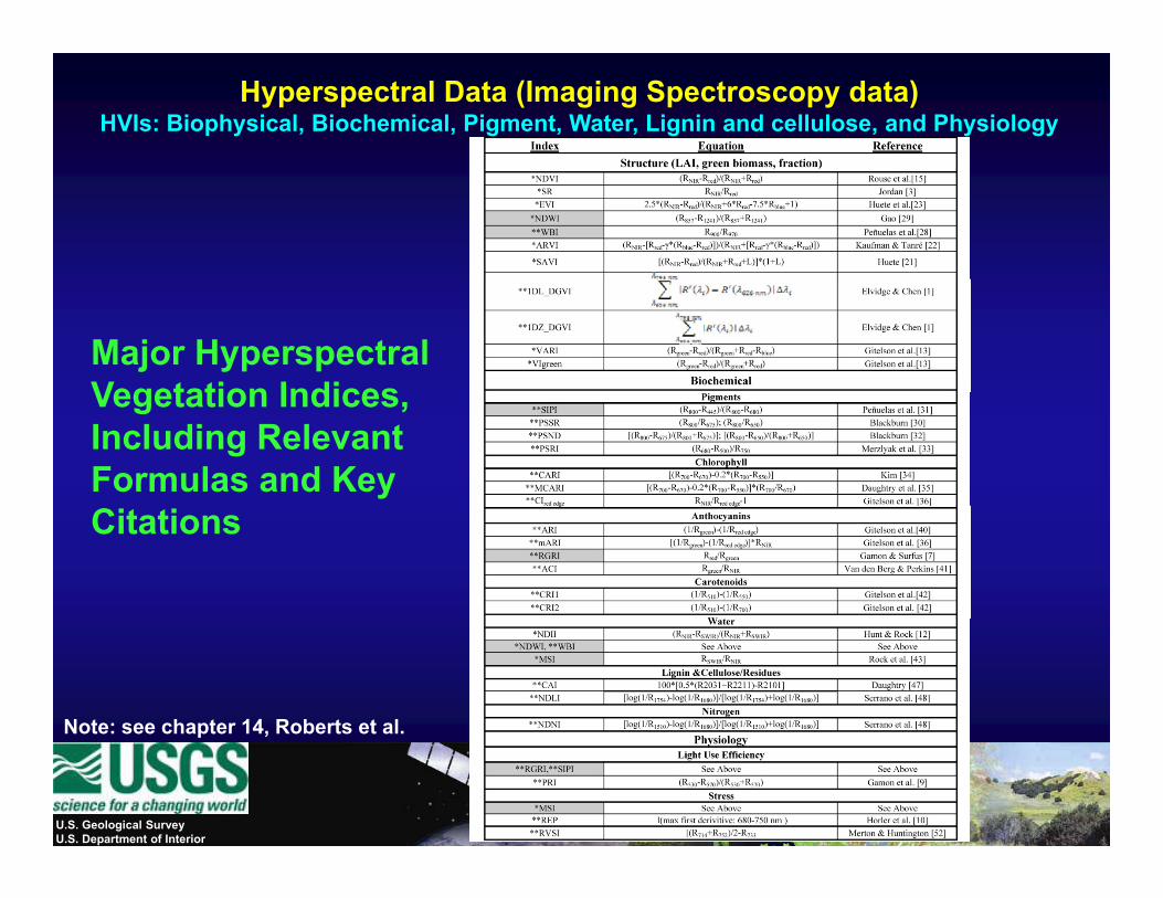
Hyperspectral Data (Imaging Spectroscopy data) HVIs: Biophysical, Biochemical, Pigment, Water, Lignin and cellulose, and Physiology
Major HyperspectralVegetation IndicesVegetation Indices, Including Relevant Formulas and Key Citations
Note: see chapter 14, Roberts et al.
U.S. Geological SurveyU.S. Department of Interior
Note: see chapter 14, Roberts et al.
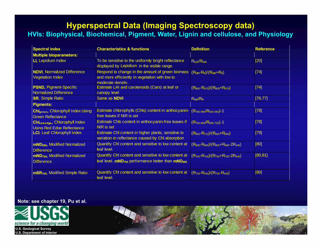
Hyperspectral Data (Imaging Spectroscopy data) HVIs: Biophysical, Biochemical, Pigment, Water, Lignin and cellulose, and Physiology
Spectral index Characteristics & functions Definition ReferenceMultiple bioparameters:LI, Lepidium Index To be sensitive to the uniformly bright reflectance
displayed by Lepidium in the visible range.R630/R586 [20]
NDVI, Normalized Difference Vegetation Index
Respond to change in the amount of green biomass and more efficiently in vegetation with low to
(RNIR-RR)/(RNIR+RR) [74]Vegetation Index and more efficiently in vegetation with low to
moderate density.PSND, Pigment-Specific Normalized Difference
Estimate LAI and carotenoids (Cars) at leaf or canopy level
(R800-R470)/(R800+R470) [74]
SR, Simple Ratio Same as NDVI RNIR/RR [76,77]Pigments:
E ti t hl h ll (Chl ) t t i th i [78]Chlgreen, Chlorophyll Index Using Green Reflectance
Estimate chlorophylls (Chls) content in anthocyanin-free leaves if NIR is set
(R760-800/R540-560)-1 [78]
Chlred-edge, Chlorophyll Index Using Red Edge Reflectance
Estimate Chls content in anthocyanin-free leaves if NIR is set
(R760-800/R690-720)-1 [78]
LCI, Leaf Chlorophyll Index Estimate Chl content in higher plants, sensitive to variation in reflectance caused by Chl absorption
(R850-R710)/(R850+R680) [79]
mND680, Modified Normalized Difference
Quantify Chl content and sensitive to low content at leaf level.
(R800-R680)/(R800+R680-2R445) [80]
mND705, Modified Normalized Difference
Quantify Chl content and sensitive to low content at leaf level. mND705 performance better than mND680
(R750-R705)/(R750+R705-2R445) [80,81]
SR M difi d Si l R ti Quantify Chl content and sensitive to low content at (R R )/(R R ) [80]
Note: see chapter 19, Pu et al.
mSR705, Modified Simple Ratio Quantify Chl content and sensitive to low content at leaf level.
(R750-R445)/(R705-R445) [80]
U.S. Geological SurveyU.S. Department of Interior
p ,
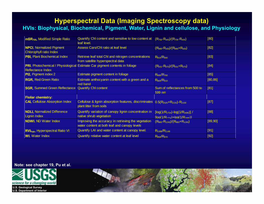
Hyperspectral Data (Imaging Spectroscopy data) HVIs: Biophysical, Biochemical, Pigment, Water, Lignin and cellulose, and Physiology
S M difi d Si l R ti Q tif Chl t t d iti t l t t t (R R )/(R R ) [80]mSR705, Modified Simple Ratio Quantify Chl content and sensitive to low content at leaf level.
(R750-R445)/(R705-R445) [80]
NPCI, Normalized Pigment Chlorophyll ratio Index
Assess Cars/Chl ratio at leaf level (R680-R430)/(R680+R430) [82]
PBI, Plant Biochemical Index Retrieve leaf total Chl and nitrogen concentrations from satellite hyperspectral data
R810/R560 [83]
PRI, Photochemical / Physiological Reflectance Index
Estimate Car pigment contents in foliage (R531-R570)/(R531+R570) [84]
PI2, Pigment index 2 Estimate pigment content in foliage R695/R760 [85]RGR, Red:Green Ratio Estimate anthocyanin content with a green and a
red bandR683/R510 [80,86]
SGR, Summed Green Reflectance Quantify Chl content Sum of reflectances from 500 to [81]SGR, Q y599 nm
[ ]
Floliar chemistry:CAI, Cellulose Absorption Index Cellulose & lignin absorption features, discriminates
plant litter from soils0.5(R2020+R2220)-R2100 [87]
NDLI, Normalized Difference Li i I d
Quantify variation of canopy lignin concentration in ti h b t ti
[log(1/R1754)-log(1/R1680)] / [88]Lignin Index native shrub vegetation [log(1/R1754)+log(1/R1680)]NDWI, ND Water Index Improving the accuracy in retrieving the vegetation
water content at both leaf and canopy levels(R860-R1240)/(R860+R1240) [89,90]
RVIhyp, Hyperspectral Ratio VI Quantify LAI and water content at canopy level. R1088/R1148 [91]
WI, Water Index Quantify relative water content at leaf level R900/R970 [92]
Note: see chapter 19, Pu et al.
U.S. Geological SurveyU.S. Department of Interior
p ,
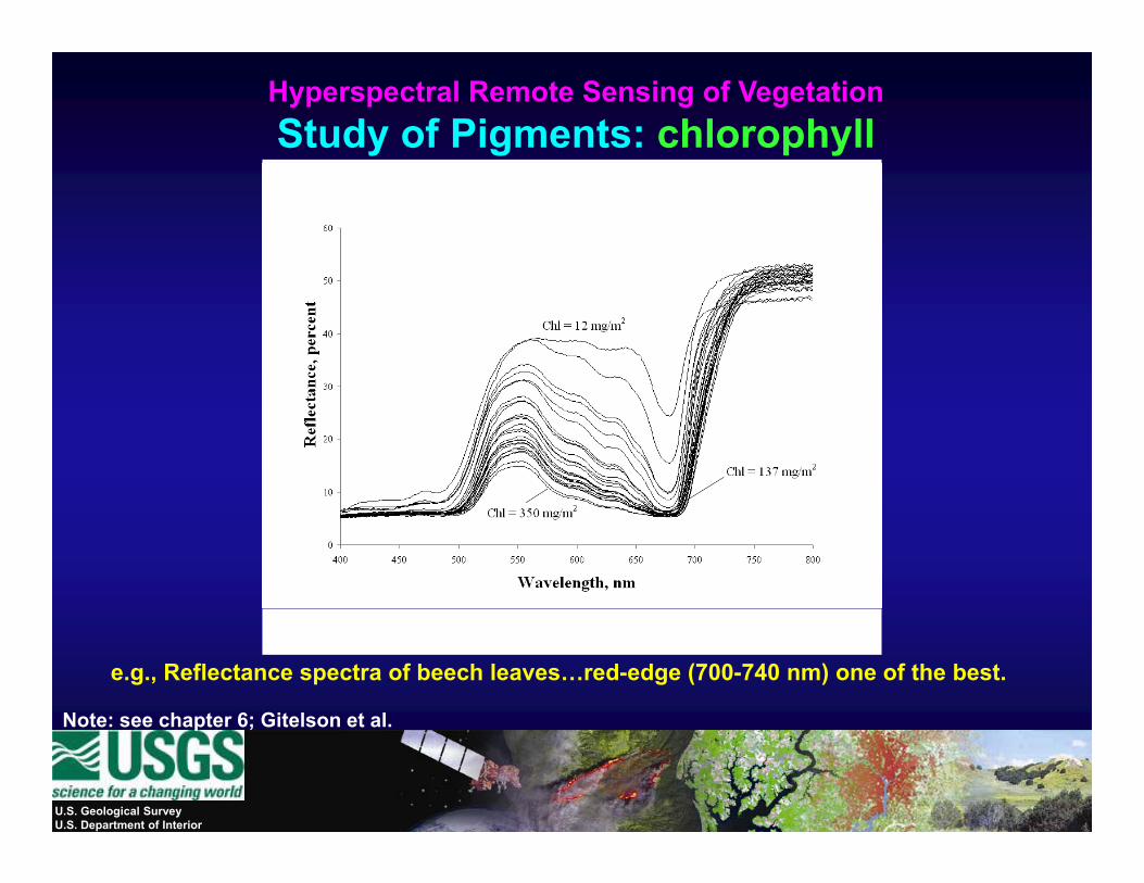
Hyperspectral Remote Sensing of Vegetation Study of Pigments: chlorophyll
Note: see chapter 6; Gitelson et al
e.g., Reflectance spectra of beech leaves…red-edge (700-740 nm) one of the best.
U.S. Geological SurveyU.S. Department of Interior
Note: see chapter 6; Gitelson et al.
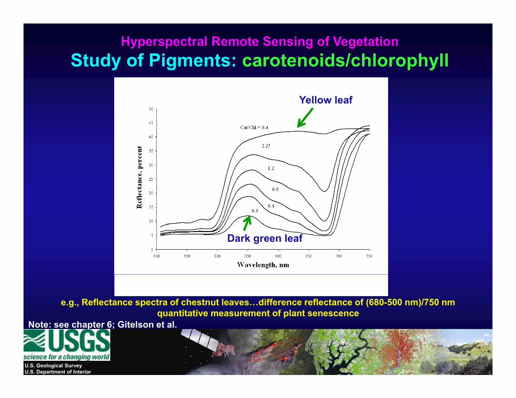
Hyperspectral Remote Sensing of Vegetation Study of Pigments: carotenoids/chlorophyll
Yellow leaf
Dark green leaf
Note: see chapter 6; Gitelson et al
e.g., Reflectance spectra of chestnut leaves…difference reflectance of (680-500 nm)/750 nm quantitative measurement of plant senescence
U.S. Geological SurveyU.S. Department of Interior
Note: see chapter 6; Gitelson et al.

Methods of Classifying Vegetation Classes or categoriesClassifying Vegetation Classes or categories Increased Accuracies over Broadband Data
U.S. Geological SurveyU.S. Department of Interior
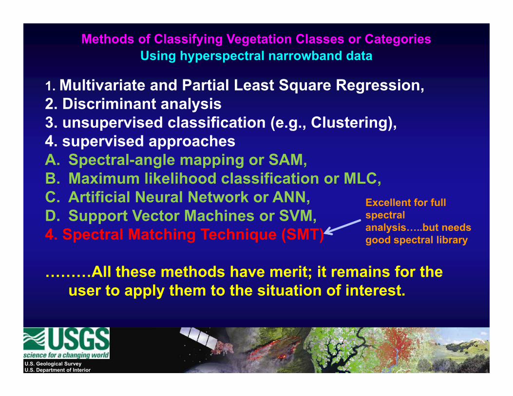
Methods of Classifying Vegetation Classes or Categories Using hyperspectral narrowband data
1. Multivariate and Partial Least Square Regression, 2. Discriminant analysis 3 unsupervised classification (e g Clustering)3. unsupervised classification (e.g., Clustering), 4. supervised approachesA. Spectral-angle mapping or SAM, B M i lik lih d l ifi ti MLCB. Maximum likelihood classification or MLC, C. Artificial Neural Network or ANN, D. Support Vector Machines or SVM,
Excellent for full spectral pp ,
4. Spectral Matching Technique (SMT)
All these methods have merit; it remains for the
analysis…..but needs good spectral library
………All these methods have merit; it remains for the user to apply them to the situation of interest.
U.S. Geological SurveyU.S. Department of Interior
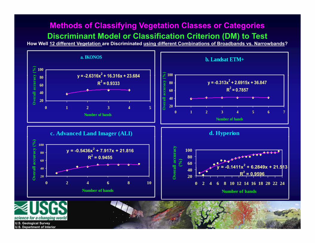
Methods of Classifying Vegetation Classes or CategoriesDiscriminant Model or Classification Criterion (DM) to Test
How Well 12 different Vegetation are Discriminated using different Combinations of Broadbands vs. Narrowbands?
a. IKONOS
y = 2 6316x2 + 16 316x + 23 684100
y (%
)
b. Landsat ETM+
100%)
How Well 12 different Vegetation are Discriminated using different Combinations of Broadbands vs. Narrowbands?
y = -2.6316x + 16.316x + 23.684R2 = 0.9333
20
40
60
80
0 1 2 3 4 5
Ove
rall
accu
racy
y = -0.313x2 + 2.6915x + 36.847R2 = 0.7857
20
40
60
80
100
vera
ll ac
cura
cy (%
0 1 2 3 4 5Number of bands
200 1 2 3 4 5 6 7
Number of bands
Ov
c. Advanced Land Imager (ALI) d. Hyperion
y = -0.5436x2 + 7.917x + 21.816R2 = 0.9455
40
60
80
100
ll ac
cura
cy (%
)
y = -0 1411x2 + 6 2849x + 21 5136080
100
all a
ccur
acy
(%)
20
40
0 2 4 6 8 10
Number of bands
Ove
ral y = -0.1411x + 6.2849x + 21.513
R2 = 0.95962040
0 2 4 6 8 10 12 14 16 18 20 22 24
Number of bands
Ove
ra
U.S. Geological SurveyU.S. Department of Interior

Concluding Thoughts I Hyperspectral (imaging Spectroscopy)Hyperspectral (imaging Spectroscopy) Knowledge Gain in Study of Vegetation
U.S. Geological SurveyU.S. Department of Interior
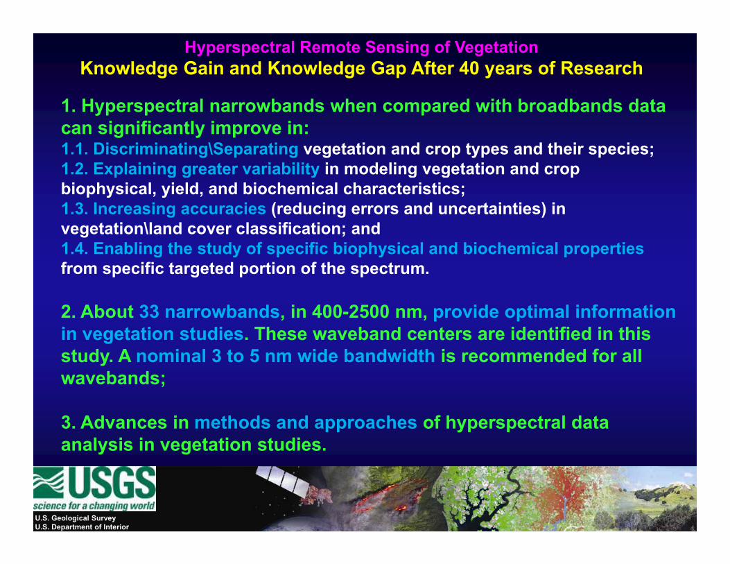
Hyperspectral Remote Sensing of Vegetation Knowledge Gain and Knowledge Gap After 40 years of Research
1 Hyperspectral narrowbands when compared with broadbands data1. Hyperspectral narrowbands when compared with broadbands data can significantly improve in:1.1. Discriminating\Separating vegetation and crop types and their species;1.2. Explaining greater variability in modeling vegetation and crop p g g y g g pbiophysical, yield, and biochemical characteristics; 1.3. Increasing accuracies (reducing errors and uncertainties) in vegetation\land cover classification; and1 4 Enabling the study of specific biophysical and biochemical properties1.4. Enabling the study of specific biophysical and biochemical properties from specific targeted portion of the spectrum.
2. About 33 narrowbands, in 400-2500 nm, provide optimal information2. About 33 narrowbands, in 400 2500 nm, provide optimal information in vegetation studies. These waveband centers are identified in this study. A nominal 3 to 5 nm wide bandwidth is recommended for all wavebands;
3. Advances in methods and approaches of hyperspectral data analysis in vegetation studies.
U.S. Geological SurveyU.S. Department of Interior
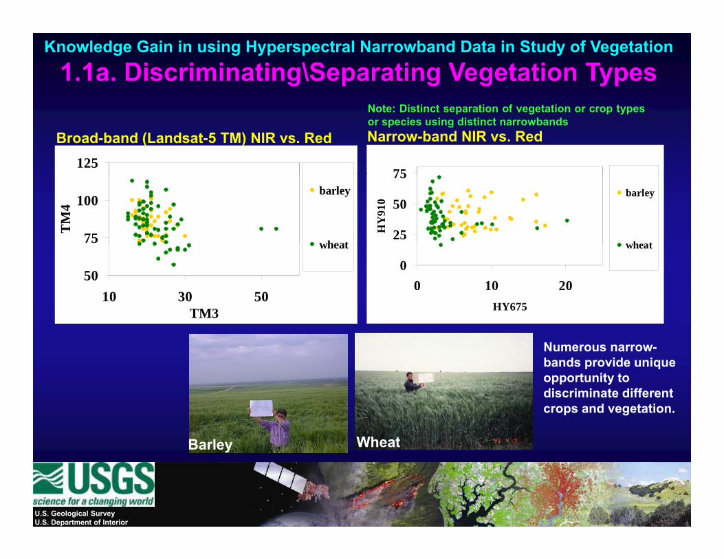
Knowledge Gain in using Hyperspectral Narrowband Data in Study of Vegetation
1.1a. Discriminating\Separating Vegetation Types
12575
Broad-band (Landsat-5 TM) NIR vs. Red Narrow-band NIR vs. Red
Note: Distinct separation of vegetation or crop typesor species using distinct narrowbands
75
100
TM
4
barley
wheat25
50
75
HY
910
barley
wheat
5010 30 50
TM3
wheat
00 10 20
HY675
wheat
TM3
Numerous narrow-bands provide unique opportunity to
WheatBarley
discriminate different crops and vegetation.
U.S. Geological SurveyU.S. Department of Interior
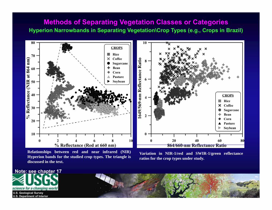
Methods of Separating Vegetation Classes or CategoriesHyperion Narrowbands in Separating Vegetation\Crop Types (e.g., Crops in Brazil)
Note: see chapter 17
Relationships between red and near infrared (NIR)Hyperion bands for the studied crop types. The triangle isdiscussed in the text.
Variation in NIR-1/red and SWIR-1/green reflectanceratios for the crop types under study.
U.S. Geological SurveyU.S. Department of Interior
Note: see chapter 17
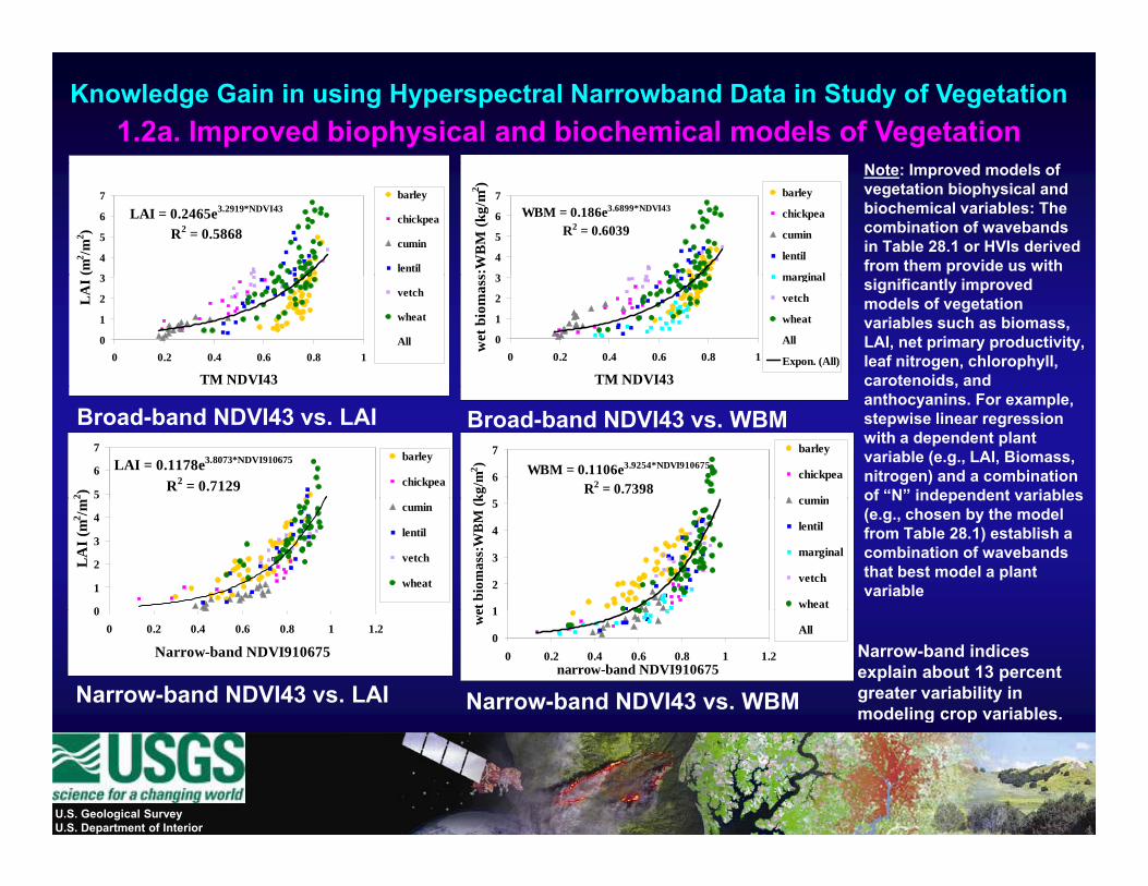
Knowledge Gain in using Hyperspectral Narrowband Data in Study of Vegetation1.2a. Improved biophysical and biochemical models of Vegetation
N I d d l f
LAI = 0.2465e3.2919*NDVI43
R2 = 0.5868
3
4
5
6
7
(m2 /m
2 )
barley
chickpea
cumin
lentil
WBM = 0.186e3.6899*NDVI43
R2 = 0.6039
3
4
5
6
7
s:W
BM
(kg/
m2 )
barley
chickpea
cumin
lentil
marginal
Note: Improved models of vegetation biophysical and biochemical variables: The combination of wavebands in Table 28.1 or HVIs derived from them provide us with
0
1
2
3
0 0.2 0.4 0.6 0.8 1
TM NDVI43
LA
I
vetch
wheat
All
E
0
1
2
3
0 0.2 0.4 0.6 0.8 1
TM NDVI43
wet
bio
mas
s marginal
vetch
wheat
All
Expon. (All)
significantly improved models of vegetation variables such as biomass, LAI, net primary productivity, leaf nitrogen, chlorophyll, carotenoids, and
LAI = 0.1178e3.8073*NDVI910675
R2 = 0.71295
6
7
2 )
barley
chickpeaWBM = 0.1106e3.9254*NDVI910675
R2 = 0.73986
7
kg/m
2 )
barley
chickpea
cumin
Broad-band NDVI43 vs. LAI Broad-band NDVI43 vs. WBM
,anthocyanins. For example, stepwise linear regression with a dependent plant variable (e.g., LAI, Biomass, nitrogen) and a combination of “N” independent variables
0
1
2
3
4
LA
I (m
2 /m cumin
lentil
vetch
wheat
1
2
3
4
5
et b
iom
ass:
WB
M (k cumin
lentil
marginal
vetch
wheat
of N independent variables (e.g., chosen by the model from Table 28.1) establish a combination of wavebands that best model a plant variable
00 0.2 0.4 0.6 0.8 1 1.2
Narrow-band NDVI9106750
1
0 0.2 0.4 0.6 0.8 1 1.2narrow-band NDVI910675
we
All
Narrow-band NDVI43 vs. LAI Narrow-band NDVI43 vs. WBM
Narrow-band indices explain about 13 percent greater variability in modeling crop variables.g p
U.S. Geological SurveyU.S. Department of Interior
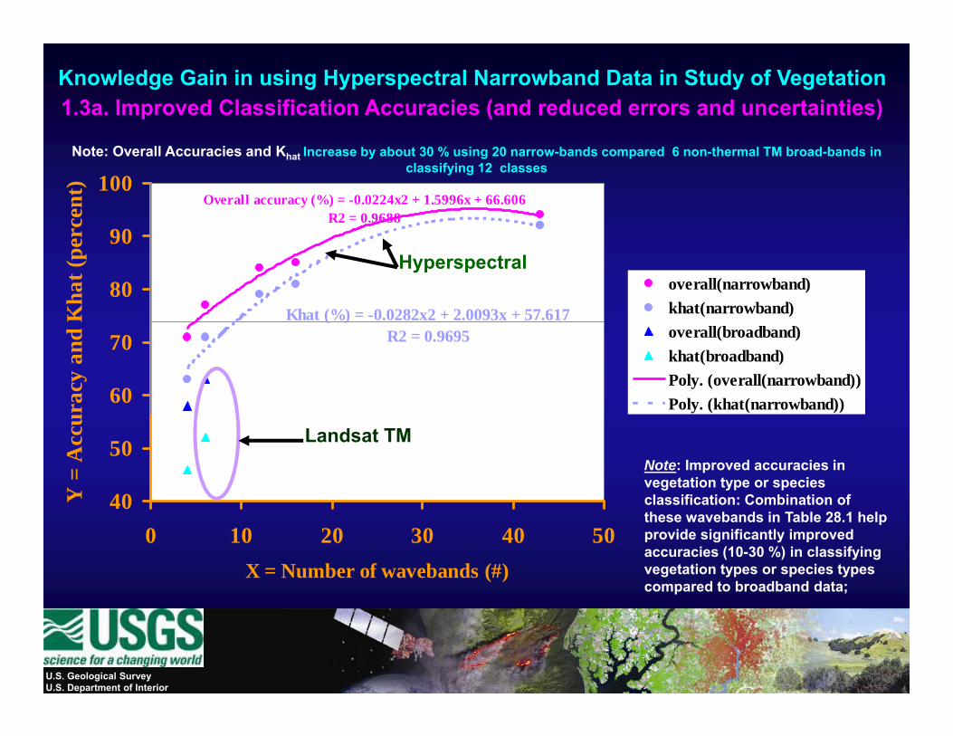
Knowledge Gain in using Hyperspectral Narrowband Data in Study of Vegetation1.3a. Improved Classification Accuracies (and reduced errors and uncertainties)
Note: Overall Accuracies and Khat Increase by about 30 % using 20 narrow-bands compared 6 non-thermal TM broad-bands in classifying 12 classes
Overall accuracy (%) = -0.0224x2 + 1.5996x + 66.606R2 = 0.9688
90
100
rcen
t)
Khat (%) = -0.0282x2 + 2.0093x + 57.61780
90
Kha
t (pe
r
overall(narrowband)khat(narrowband)
Hyperspectral
( )R2 = 0.9695
60
70
urac
y an
d K
overall(broadband)khat(broadband)Poly. (overall(narrowband))Poly. (khat(narrowband))
40
50
Y =
Acc
u
Landsat TMNote: Improved accuracies in vegetation type or species classification: Combination of 40
0 10 20 30 40 50X = Number of wavebands (#)
these wavebands in Table 28.1 help provide significantly improved accuracies (10-30 %) in classifying vegetation types or species types compared to broadband data;
U.S. Geological SurveyU.S. Department of Interior

Knowledge Gain in using Hyperspectral Narrowband Data in Study of Vegetation1.3b. Improved Classification Accuracies (and reduced errors and uncertainties)
0.7
Stepwise Discriminant Analysis (SDA)- Wilks’ Lambda to Test : How Well Different Forest Vegetation are Discriminated from One Another
Lesser the Wilks’ Lambda greater is
0.5
0.6
Fallow
the seperability. Note that beyond 10-20 wavebands Wilks’ Lambda
becomes asymptotic.
0.3
0.4
ilk's
lam
bda
Fallow
Primary forest
1-3 yr vs. 3-5 yr vs. 5-8 yr
Pristine vs. degraded
0.1
0.2
Wi
Secondary forestYoung vs. mature vs. mixed
0
1 4 7 10 13 16 19 22 25Number of bands
Primary + secondaryforests + fallow areas
All above
U.S. Geological SurveyU.S. Department of Interior
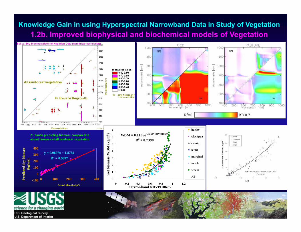
Knowledge Gain in using Hyperspectral Narrowband Data in Study of Vegetation1.2b. Improved biophysical and biochemical models of Vegetation
7 barley
21 bands predicting biomass compared to actual biomass of all rainforest vegetation
y = 0.9697x + 1.8784R2 = 0.9697
200
300
400
biom
ass
2)
WBM = 0.1106e3.9254*NDVI910675
R2 = 0.7398
3
4
5
6
7
ass:
WB
M (k
g/m
2 )
b ey
chickpea
cumin
lentil
marginal
-100
0
100
200
0 100 200 300 400Actual dbm (kg/m2)
Pred
icte
d dr
y (k
g/m
2
0
1
2
0 0.2 0.4 0.6 0.8 1 1.2narrow-band NDVI910675
wet
bio
ma
vetch
wheat
All
U.S. Geological SurveyU.S. Department of Interior
Concluding Thoughts II Hyperspectral (imaging Spectroscopy)Hyperspectral (imaging Spectroscopy)
Potential Products in Study of Vegetation
U.S. Geological SurveyU.S. Department of Interior
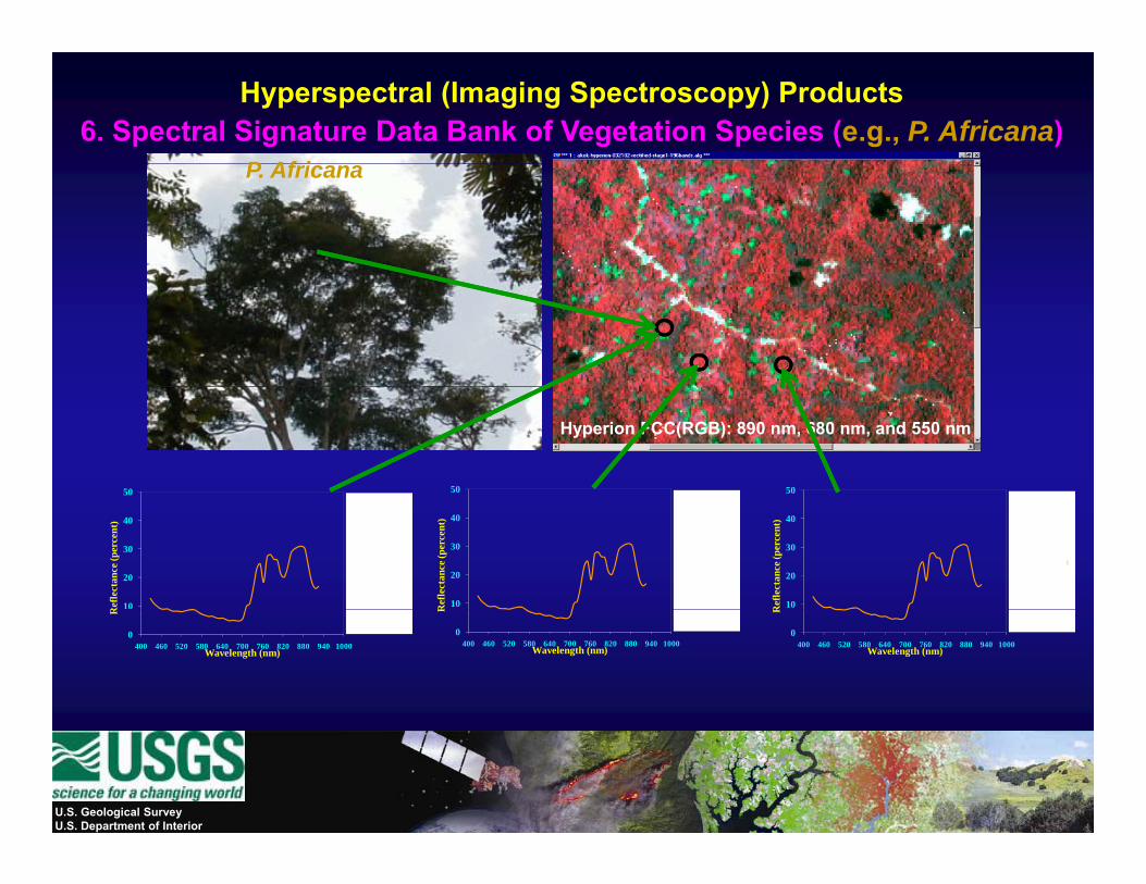
Hyperspectral (Imaging Spectroscopy) Products 6. Spectral Signature Data Bank of Vegetation Species (e.g., P. Africana)
P Af iP. Africana
50
Hyperion FCC(RGB): 890 nm, 680 nm, and 550 nm
50 50
10
20
30
40
Ref
lect
ance
(per
cent
)
Y. sec. Forest
10
20
30
40
Ref
lect
ance
(per
cent
)
Y. sec. Forest
10
20
30
40
Ref
lect
ance
(per
cent
)
Y. sec. Forest
0400 460 520 580 640 700 760 820 880 940 1000
R
Wavelength (nm)
0400 460 520 580 640 700 760 820 880 940 1000
R
Wavelength (nm)
0400 460 520 580 640 700 760 820 880 940 1000
R
Wavelength (nm)
U.S. Geological SurveyU.S. Department of Interior
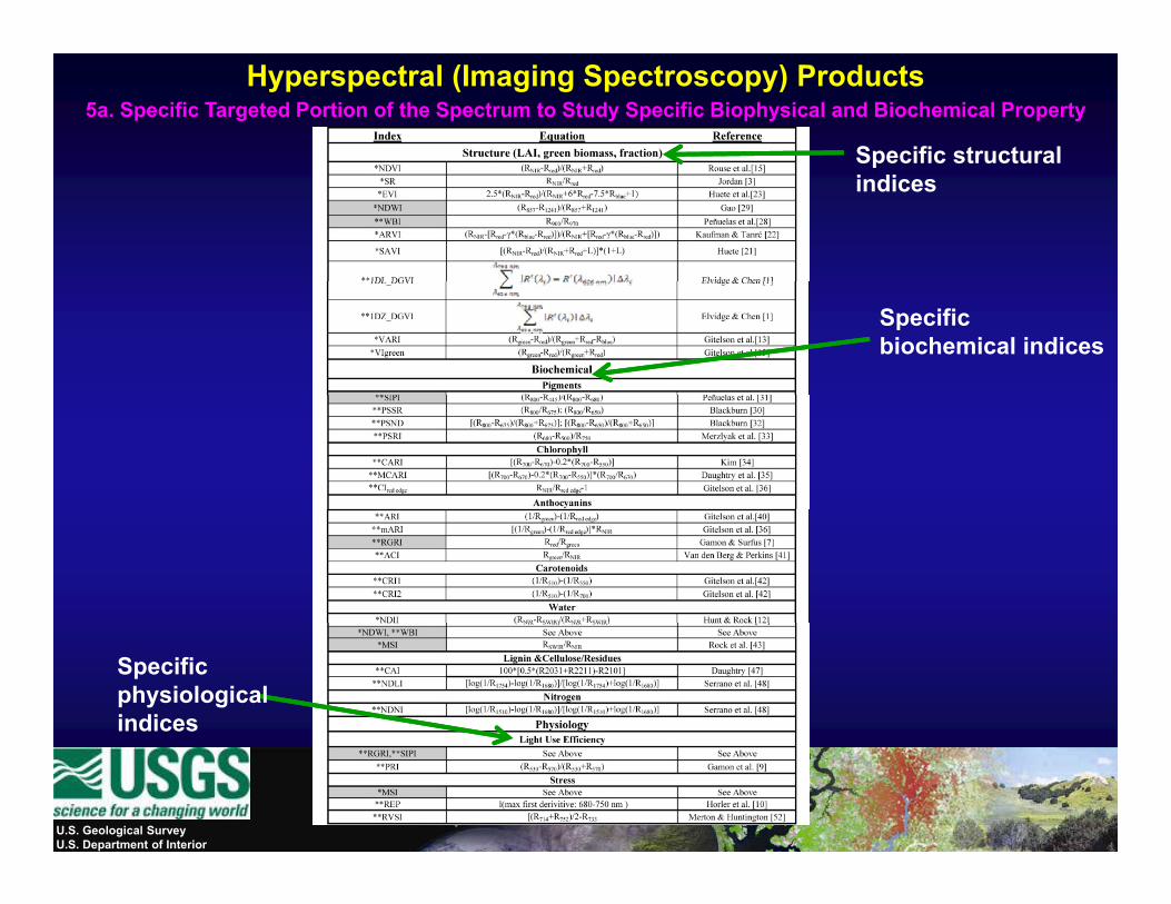
Hyperspectral (Imaging Spectroscopy) Products 5a. Specific Targeted Portion of the Spectrum to Study Specific Biophysical and Biochemical Property
Specific structural pindices
Specific biochemical indices
Specific physiological indices
U.S. Geological SurveyU.S. Department of Interior
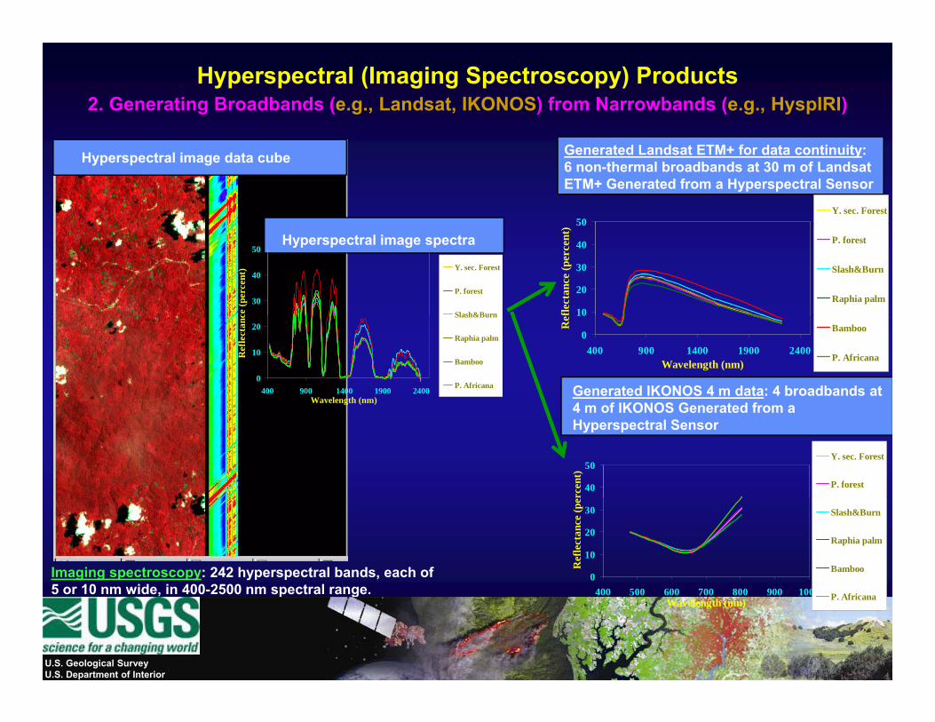
Hyperspectral (Imaging Spectroscopy) Products 2. Generating Broadbands (e.g., Landsat, IKONOS) from Narrowbands (e.g., HyspIRI)
50Y. sec. Forest
Generated Landsat ETM+ for data continuity: 6 non-thermal broadbands at 30 m of Landsat ETM+ Generated from a Hyperspectral Sensor
Hyperspectral image data cube
30
40
50ce
(per
cent
) Y. sec. Forest
P. forest
Slash&Burn 10
20
30
40
50
flect
ance
(per
cent
)
P. forest
Slash&Burn
Raphia palm
Hyperspectral image spectra
0
10
20
400 900 1400 1900 2400Wavelength (nm)
Ref
lect
anc Slash&Burn
Raphia palm
Bamboo
P. Africana
0
10
400 900 1400 1900 2400Wavelength (nm)
Re
Bamboo
P. Africana
Generated IKONOS 4 m data: 4 broadbands at 4 m of IKONOS Generated from a
40
50
rcen
t)
Y. sec. Forest
P. forest
4 m of IKONOS Generated from a Hyperspectral Sensor
0
10
20
30
400 500 600 700 800 900 1000R
efle
ctan
ce (p
er
Slash&Burn
Raphia palm
BambooImaging spectroscopy: 242 hyperspectral bands, each of 5 or 10 nm wide in 400 2500 nm spectral range 400 500 600 700 800 900 1000
Wavelength (nm) P. Africana5 or 10 nm wide, in 400-2500 nm spectral range.
U.S. Geological SurveyU.S. Department of Interior
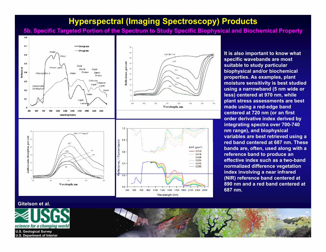
Hyperspectral (Imaging Spectroscopy) Products 5b. Specific Targeted Portion of the Spectrum to Study Specific Biophysical and Biochemical Property
It is also important to know what specific wavebands are most suitable to study particular biophysical and/or biochemical properties. As examples, plantproperties. As examples, plant moisture sensitivity is best studied using a narrowband (5 nm wide or less) centered at 970 nm, while plant stress assessments are best made using a red-edge band centered at 720 nm (or an first order derivative index derived by integrating spectra over 700-740 nm range), and biophysical variables are best retrieved using a red band centered at 687 nm Thesered band centered at 687 nm. These bands are, often, used along with a reference band to produce an effective index such as a two-band normalized difference vegetation index involving a near infrared
Gitelson et al.
g(NIR) reference band centered at 890 nm and a red band centered at 687 nm.
U.S. Geological SurveyU.S. Department of Interior
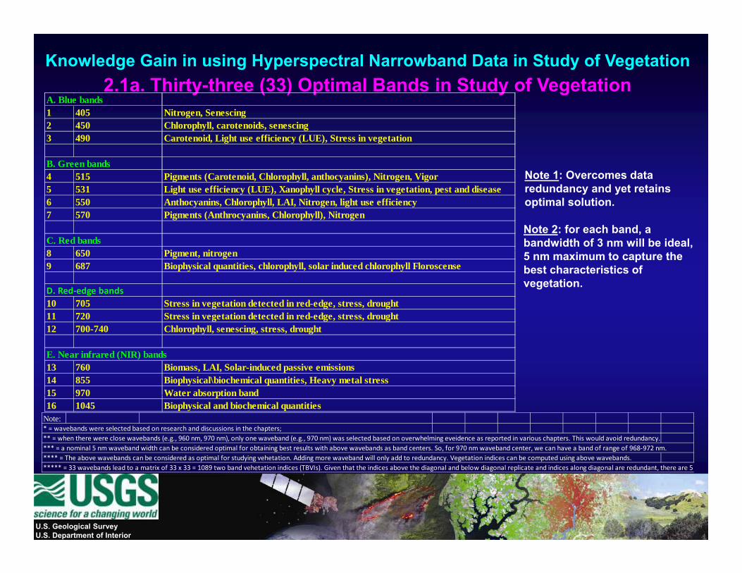
Knowledge Gain in using Hyperspectral Narrowband Data in Study of Vegetation2.1a. Thirty-three (33) Optimal Bands in Study of Vegetation
A. Blue bands1 405 Nitrogen, Senescing2 450 Chlorophyll, carotenoids, senescing 3 490 Carotenoid, Light use efficiency (LUE), Stress in vegetation
B. Green bands4 515 Pigments (Carotenoid, Chlorophyll, anthocyanins), Nitrogen, Vigor Note 1: Overcomes data4 515 Pigments (Carotenoid, Chlorophyll, anthocyanins), Nitrogen, Vigor 5 531 Light use efficiency (LUE), Xanophyll cycle, Stress in vegetation, pest and disease 6 550 Anthocyanins, Chlorophyll, LAI, Nitrogen, light use efficiency7 570 Pigments (Anthrocyanins, Chlorophyll), Nitrogen
C. Red bands8 650 Pi t it
Note 2: for each band, a bandwidth of 3 nm will be ideal,
Note 1: Overcomes data redundancy and yet retains optimal solution.
8 650 Pigment, nitrogen9 687 Biophysical quantities, chlorophyll, solar induced chlorophyll Floroscense
D. Red‐edge bands10 705 Stress in vegetation detected in red-edge, stress, drought11 720 Stress in vegetation detected in red-edge, stress, drought
5 nm maximum to capture the best characteristics of vegetation.
12 700-740 Chlorophyll, senescing, stress, drought
E. Near infrared (NIR) bands13 760 Biomass, LAI, Solar-induced passive emissions14 855 Biophysical\biochemical quantities, Heavy metal stress15 970 Water absorption band15 970 Water absorption band16 1045 Biophysical and biochemical quantities
Note:* = wavebands were selected based on research and discussions in the chapters;** = when there were close wavebands (e.g., 960 nm, 970 nm), only one waveband (e.g., 970 nm) was selected based on overwhelming eveidence as reported in various chapters. This would avoid redundancy.*** = a nominal 5 nm waveband width can be considered optimal for obtaining best results with above wavebands as band centers. So, for 970 nm waveband center, we can have a band of range of 968‐972 nm.**** = The above wavebands can be considered as optimal for studying vehetation. Adding more waveband will only add to redundancy. Vegetation indices can be computed using above wavebands.***** = 33 wavebands lead to a matrix of 33 x 33 = 1089 two band vehetation indices (TBVIs) Given that the indices above the diagonal and below diagonal replicate and indices along diagonal are redundant there are 52***** = 33 wavebands lead to a matrix of 33 x 33 = 1089 two band vehetation indices (TBVIs). Given that the indices above the diagonal and below diagonal replicate and indices along diagonal are redundant, there are 52
U.S. Geological SurveyU.S. Department of Interior
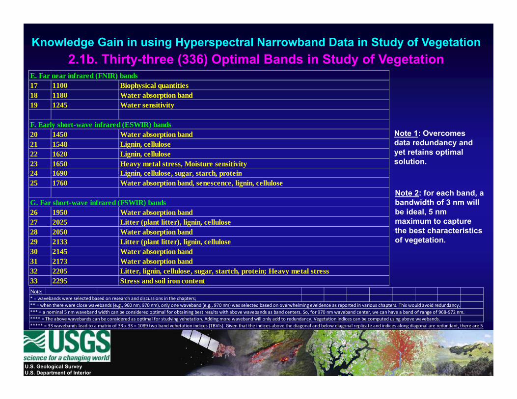
Knowledge Gain in using Hyperspectral Narrowband Data in Study of Vegetation2.1b. Thirty-three (336) Optimal Bands in Study of Vegetation
E F i f d (FNIR) b dE. Far near infrared (FNIR) bands17 1100 Biophysical quantities18 1180 Water absorption band19 1245 Water sensitivity
F Early short wave infrared (ESWIR) bandsF. Early short-wave infrared (ESWIR) bands20 1450 Water absorption band21 1548 Lignin, cellulose22 1620 Lignin, cellulose23 1650 Heavy metal stress, Moisture sensitivity24 1690 Lignin cellulose sugar starch protein
Note 1: Overcomes data redundancy and yet retains optimal solution.
Note 2: for each band, a bandwidth of 3 nm will be ideal, 5 nm maximum to capture
24 1690 Lignin, cellulose, sugar, starch, protein25 1760 Water absorption band, senescence, lignin, cellulose
G. Far short-wave infrared (FSWIR) bands26 1950 Water absorption band27 2025 Litter (plant litter), lignin, cellulose p
the best characteristics of vegetation.
(p ), g ,28 2050 Water absorption band29 2133 Litter (plant litter), lignin, cellulose30 2145 Water absorption band31 2173 Water absorption band32 2205 Litter, lignin, cellulose, sugar, startch, protein; Heavy metal stressg g p y33 2295 Stress and soil iron contentNote:* = wavebands were selected based on research and discussions in the chapters;** = when there were close wavebands (e.g., 960 nm, 970 nm), only one waveband (e.g., 970 nm) was selected based on overwhelming eveidence as reported in various chapters. This would avoid redundancy.*** = a nominal 5 nm waveband width can be considered optimal for obtaining best results with above wavebands as band centers. So, for 970 nm waveband center, we can have a band of range of 968‐972 nm.**** = The above wavebands can be considered as optimal for studying vehetation. Adding more waveband will only add to redundancy. Vegetation indices can be computed using above wavebands.***** = 33 wavebands lead to a matrix of 33 x 33 = 1089 two band vehetation indices (TBVIs) Given that the indices above the diagonal and below diagonal replicate and indices along diagonal are redundant there are 52***** = 33 wavebands lead to a matrix of 33 x 33 = 1089 two band vehetation indices (TBVIs). Given that the indices above the diagonal and below diagonal replicate and indices along diagonal are redundant, there are 52
U.S. Geological SurveyU.S. Department of Interior
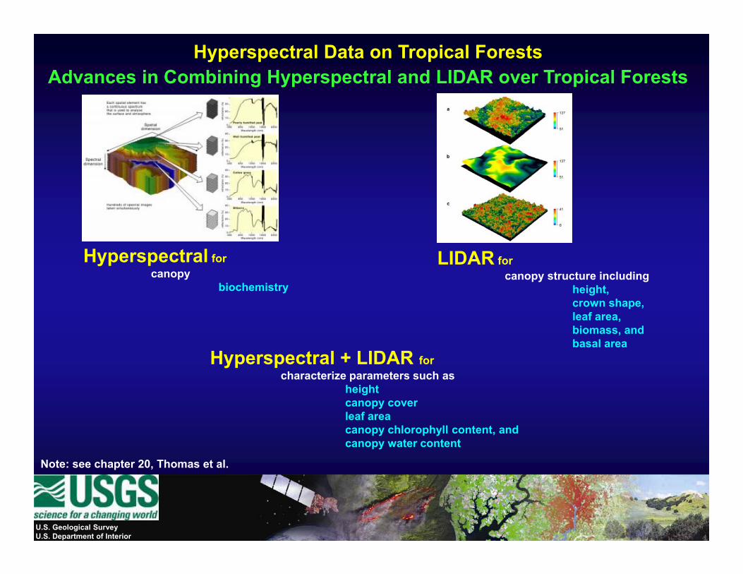
Hyperspectral Data on Tropical ForestsAdvances in Combining Hyperspectral and LIDAR over Tropical Forests
H t l LIDAR forcanopy structure including
height, crown shape, leaf area,
Hyperspectral forcanopy
biochemistry
biomass, and basal area
Hyperspectral + LIDAR forcharacterize parameters such as
height
Note: see chapter 20, Thomas et al.
canopy coverleaf areacanopy chlorophyll content, and canopy water content
U.S. Geological SurveyU.S. Department of Interior
p ,
Publications Hyperspectral Remote Sensing of Vegetation
U.S. Geological SurveyU.S. Department of Interior

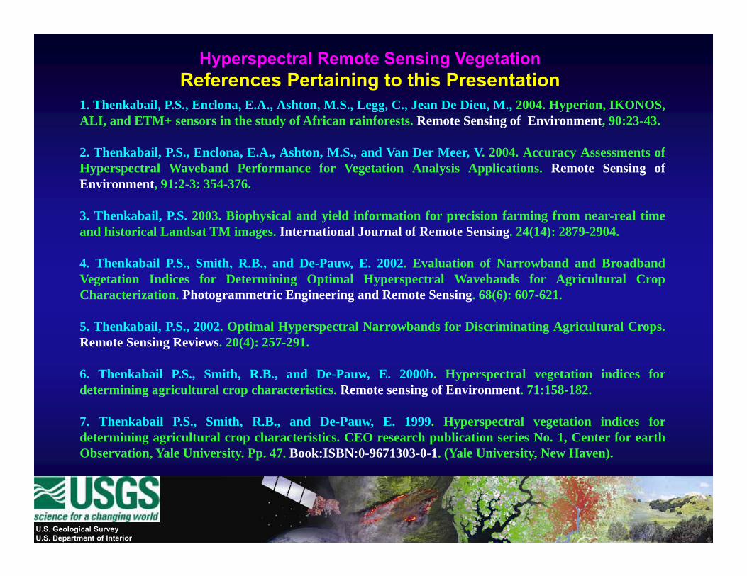
Hyperspectral Remote Sensing Vegetation References Pertaining to this Presentation
Thenkabail, P.S., Lyon, G.J., and Huete, A. 2011. Book entitled: “Hyperspectral Remote Sensing ofVegetation”. 28 Chapters. CRC Press- Taylor and Francis group, Boca Raton, London, New York. Pp.700+ (80+ pages in color). To be published by October 31, 2011.
U.S. Geological SurveyU.S. Department of Interior
Hyperspectral Remote Sensing Vegetation References Pertaining to this Presentation
1 Thenkabail P S Enclona E A Ashton M S Legg C Jean De Dieu M 2004 Hyperion IKONOS1. Thenkabail, P.S., Enclona, E.A., Ashton, M.S., Legg, C., Jean De Dieu, M., 2004. Hyperion, IKONOS,ALI, and ETM+ sensors in the study of African rainforests. Remote Sensing of Environment, 90:23-43.
2. Thenkabail, P.S., Enclona, E.A., Ashton, M.S., and Van Der Meer, V. 2004. Accuracy Assessments ofHyperspectral Waveband Performance for Vegetation Analysis Applications. Remote Sensing ofEnvironment, 91:2-3: 354-376.
3. Thenkabail, P.S. 2003. Biophysical and yield information for precision farming from near-real timeand historical Landsat TM images. International Journal of Remote Sensing. 24(14): 2879-2904.
4. Thenkabail P.S., Smith, R.B., and De-Pauw, E. 2002. Evaluation of Narrowband and BroadbandVegetation Indices for Determining Optimal Hyperspectral Wavebands for Agricultural CropCharacterization. Photogrammetric Engineering and Remote Sensing. 68(6): 607-621.
5 Th k b il P S 2002 O ti l H t l N b d f Di i i ti A i lt l C5. Thenkabail, P.S., 2002. Optimal Hyperspectral Narrowbands for Discriminating Agricultural Crops.Remote Sensing Reviews. 20(4): 257-291.
6. Thenkabail P.S., Smith, R.B., and De-Pauw, E. 2000b. Hyperspectral vegetation indices fordetermining agricultural crop characteristics. Remote sensing of Environment. 71:158-182.
7. Thenkabail P.S., Smith, R.B., and De-Pauw, E. 1999. Hyperspectral vegetation indices fordetermining agricultural crop characteristics. CEO research publication series No. 1, Center for earthObservation, Yale University. Pp. 47. Book:ISBN:0-9671303-0-1. (Yale University, New Haven).
U.S. Geological SurveyU.S. Department of Interior