Hybridization of Harmonic Search Algorithm InTraining Radial Basis Function With Dynamic DecayAdjustment For Condition MonitoringHue Yee CHONG 

University of Malaya: Universiti MalayaShing Chiang TAN 

Multimedia University - Melaka Campus: Multimedia UniversityHwa Jen Yap  ( hjyap737@um.edu.my )

University of Malaya https://orcid.org/0000-0001-7637-9297

Research Article

Keywords: Metaheuristic, Radial Basis Function Network, condition monitoring, Harmony Search,Optimization

Posted Date: April 30th, 2021

DOI: https://doi.org/10.21203/rs.3.rs-174329/v1

License: This work is licensed under a Creative Commons Attribution 4.0 International License.  Read Full License

HYBRIDIZATION OF HARMONIC SEARCH

ALGORITHM IN TRAINING RADIAL BASIS

FUNCTION WITH DYNAMIC DECAY ADJUSTMENT

FOR CONDITION MONITORING

Hue Yee CHONG 1, Shing Chiang TAN 2, and Hwa Jen YAP 1*

( 1Department of Mechanical Engineering, Faculty of Engineering, University Malaya, Kuala Lumpur 50603,

Malaysia

2Faculty of Information Science & Technology, Multimedia University, Melaka 75450, Malaysia)

*Corresponding author

Name: Hwa Jen YAP

Tel: +603-7967 5240 (Office)

Fax: +603-7957 5317

Email address: hjyap737@um.edu.my

Abstract: In recent decades, hybridization of superior attributes of few algorithms was proposed to aid in covering

more areas of complex application as well as improves performance. This paper presents an intelligent system

integrating a Radial Basis Function Network with Dynamic Decay Adjustment (RBFN-DDA) with a Harmony

Search (HS) to perform condition monitoring in industrial processes. An effective condition monitoring can help

reduce unexpected breakdown incidents and facilitate in maintenance. RBDN-DDA performs incremental

learning wherein its structure expands by adding new hidden units to include new information. As such, its training

can reach stability in a shorter time compared to the gradient-descent based methods. By integrating with the HS

algorithm, the proposed metaheuristic neural network (RBFN-DDA-HS) can optimize the RBFN-DDA

parameters and improve classification performances from the original RBFN-DDA by 2.2% up to 22.5% in two

benchmarks and a real-world condition-monitoring case studies. The results also show that the proposed RBFN-

DDA-HS is compatible, if not better than, the classification performances of other state-of-art machine learning

methods.

Keywords: Metaheuristic, Radial Basis Function Network, condition monitoring, Harmony Search, Optimization

Declarations:

Funding: The authors would like to acknowledge the Ministry of Higher Education of Malaysia for the financial support under

the Fundamental Research Grant Scheme (FRGS), Grant No: FP061-2015A and also the Ministry of Education Malaysia for

the financial support under the program myBrain15.

Conflict of Interest: The authors declare that there is no conflict of interests regarding the publication of this paper.

Availability of data and material: NA

Code availability: NA

Authors' contributions: NA

1. Introduction

Maintenance involves carrying out all technical and associated administrative activities to keep all components in

an operational system to perform their function properly [1]. If any equipment breakdown occurs in a well-

maintained operational system, minor problems can be detected and corrected by conducting short daily

inspection, cleaning and lubricating activities. An effective maintenance action requires company-wide

participation and support by every personnel in order to make plant and equipment more reliable [2].

Basically, maintenance can be divided into two types, preventive maintenance and corrective maintenance [3].

Preventive maintenance includes all planned maintenance actions e.g. periodic inspection, condition monitoring

etc. that are implemented to avoid equipment from breaking down unexpectedly. Corrective maintenance includes

all planned and unplanned maintenance actions to rectify failures before restoring equipment back to its

operational condition. Condition monitoring is a major component in predictive maintenance which monitors the

condition and the significant changes of the machinery parameter to perform early detection and eliminate

equipment defects that could cause unplanned downtime or incur unnecessary expenditures [4]. It is essential to

develop efficient condition monitoring techniques for (1) quickly identifying the faulty components before

breakdown. (2) reducing costly repairs caused by unexpected failure. (3) optimizing the scheduling of preventive

and predictive maintenance operations without routine inspections, which may require periodic shutdowns in a

plant. Condition monitoring consists of two sequential processes: feature extraction and condition classification

[5]. Feature extraction requires the use of signal processing and/or post processing techniques; it is a mapping

process from the signal space to the feature space. The condition classification is a process of classifying the

obtained features into different categories. The traditional approach of condition monitoring relies on human

expertise to relate the extracted features to the faults, which is usually time-consuming and unreliable, particularly

when multiple features are referred for fault diagnostics and when the data are affected by noises [6]. Fault

diagnosis coupled with artificial intelligence (AI) can potentially overcome the shortcoming of traditional signal

processing techniques by incorporating the human-like thought abilities such as learning, reasoning and self-

correction [7]. The widely used AI tools in condition monitoring include artificial neural network (ANN), fuzzy

logic system, support vector machine, extreme learning machine and etc. [8]. Literature shows that ANNs with

learning capabilities are useful models for tackling condition based maintenance problems [9]. They learn from

data samples without a requirement for building an exact mathematical model. However, the performance of

ANNs is highly depended on their parameter settings. For this concern, numerous global optimization methods

are introduced and utilized to train ANNs to achieve a better network performance. Many of these global

optimization methods are metaheuristic algorithms, which initiate a search process to explore in the search space

to obtain near optimal solutions. The metaheuristic algorithms are mechanisms that imitate certain strategies

inspired from nature, social behavior, physical laws, etc. Literature showed that many metaheuristic algorithms

have been successfully used to optimize the ANN’s design and the parameters [10]. Many reviews on ANN based

condition monitoring have been presented [11, 12]. Notably, the application of evolutionary ANNs to condition

monitoring is still relatively few. An effective evolutionary ANN-based condition monitoring model is helpful to

reduce the frequency of unexpected breakdown incidents and thus, facilitate in maintenance. Thus, this motivates

a research on developing an autonomous learning model based on the hybridization of an adaptive ANN and a

metaheuristic algorithm for handling condition classification tasks in industries, such as in power systems. In this

paper, a hybrid model of an incremental radial basis ANN and metaheuristic algorithm is developed. A

metaheuristic algorithm (i.e., harmony search (HS) algorithm) is proposed to improve the learning parameters of

the ANN. The research work is aimed at developing an evolutionary ANN for monitoring operating states of a

system more accurately in a power plant.

After Section 1, the Section 2 of this paper will present a review of condition monitoring and fault diagnosis

techniques. In addition, the state of art of ANN and evolutionary ANN models used for performing condition

monitoring and fault detection will be described. The proposed evolutionary ANN model will be described in

Section 3. The details of machine learning components (namely, Radial Basis Function Network with Dynamic

Decay Adjustment (RBFN-DDA), Harmony Search (HS)) will be also presented before describing the proposed

RBFN-DDA-HS in details. Section 4 reports and analyzes results in an experimental study involving condition

monitoring on a circulating water system in a power plant. Finally, Section 5 draws concluding remarks and

suggestions for further work.

2. Related Work

2.1 Condition Monitoring and Fault Detection Techniques

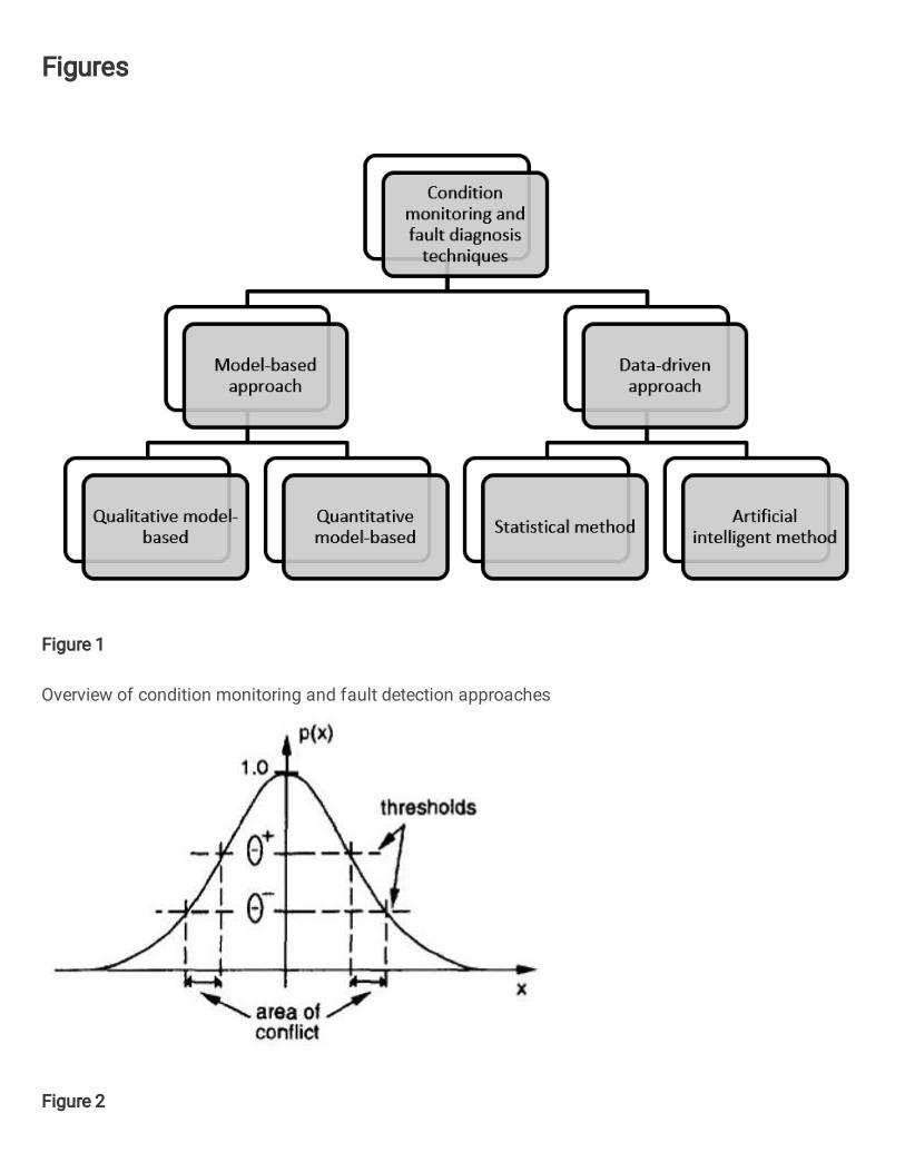
In general, condition monitoring and fault detection techniques can be broadly classified into model-based

approach [13] and data-driven approach [14], which are shown in Figure 1. Many review articles are available to

survey the application of techniques from data-driven and model-based approaches in process monitoring and

fault detection [15-17]. The model-based approach involves a modeling process, which is based on fundamental

understanding about the physics of the process. The model can be either of a qualitative or a quantitative type.

Qualitative modeling [18] relies on the use of qualitative functions centered around different units in a process to

express the relationship between the input and output of the system while quantitative modeling [19] is built by

the use of mathematical function. The performance and reliability of the diagnostic system are assessed by the

accuracy of the model. Thus, these approaches are usually applied only when an accurate analytical model is

available. However, an accurate mathematical model is usually difficult to derive to represent complex mechanical

systems, especially when the machines operate in uncertain and noisy environments [20]. Besides, model-based

approaches also rely on human expertise to relate the extracted features to the faults, which is usually time-

consuming and unreliable, particularly when multiple features are utilized for fault diagnostics and when the data

are affected by noises [6]. Data-driven approach overcomes the above mentioned limitation of the model-based

approaches and is more viable to monitor industrial processes that are inherently automated. Data-driven approach

requires for real data obtained from a data acquisition system to monitor or forecast the process behaviour of the

system under monitoring. The commonly used data-driven methods can be divided into statistical [21] and AI

approaches [8]. Methods under the statistical approach perform condition monitoring / fault detection by

identifying the relationships among the data and these relationships are referred for making classification and

prediction in the future. The commonly used statistical methods such as control chart, principle component

analysis and partial least squares are easy to build and they can provide fast detection on abnormal situations [22].

To further improve the diagnosis performance, fault diagnosis coupled with AI with the human-like thought

abilities such as learning, reasoning and self-correction [7] are extensively developed. Comprehensive reviews on

the use of AI techniques for fault detection and condition monitoring on mechanical components such as induction

machine [11] and planetary gearboxes [12] have been presented. The reviews show AI is useful to enhance the

precision and accuracy of the condition monitoring / fault detection system. AI condition monitoring / fault

detection systems have been developed by using, for examples, ANN, fuzzy logic system, support vector machine,

extreme learning machine and etc. [8]. Among them, ANN is popular due to its capability of identifying the

complex nonlinear relationships among features in a large dataset and hence, it can perform with an accurate

prediction.

Figure 1: Overview of condition monitoring and fault detection approaches

2. 2 ANN and Evolutionary Neural Network Methods for Condition Monitoring and Fault Detection

ANNs have been widely applied as condition classification tool in combination with signal processing techniques

for feature extraction. For example, bearing has been identified as one of the main fault components in rotating

machinery. From the literature, extensive research work on bearing fault detection and diagnosis have been

reported [23]. A single hidden layer feed forward ANN was proposed to perform health diagnostics of ball

bearings in direct-drive motors [24]. The feed forward ANN overcomes the problem of continuous change in

rotational speed of the motor and identifies the health of ball bearing in different speed applications. A singular

spectrum analysis (SSA) is integrated with an ANN based classifier to perform fault detection and diagnosis [25].

Feature extraction by using existing time series methods could be affected by noise and sample sizes, but the

proposed method could overcome the drawback of the existing time series methods and achieve a high

classification rate. A feature extraction method based on empirical mode decomposition (EMD) was appended to

an ANN based classifier to categorize bearing defects [26]. The authors showed that the ANN can perform

degradation assessment on the bearing condition automatically without human intervention. Kankar et.al

compared the effectiveness of ANN and support vector machine (SVM) in detecting faults in a rotor bearing

system [27]. They used statistical methods to extract features that were input to both ANN and SVM classifiers.

Results showed that ANN classifier was able to achieve higher accuracy than SVM. An adaptive algorithm based

on wavelet transform was applied to perform feature extraction and extracted features were input to ANN and

KNN, where ANN showed more effective in classifying bearing faults [28]. Effective condition monitoring

technique is useful to enhance a machining process. Siddhpura et.al presented a review of different classifiers

(such as ANN, fuzzy logic, neurofuzzy, hidden markov model and SVM) used for predicting tool wear in metal

cutting such [29]. Among them, ANN classifier was the most frequently used classifier due to its noise tolerant

and high fault adaptability characteristics. A hybrid machine-learning classifier between Gaussian classifier and

an adaptive resonance theory (ART) neural network was proposed to implement online tool wear monitoring [30].

This hybrid machine-learning classifier could memorize new knowledge in online training and achieve high

classification accuracy. The performance of an ANN classifier was demonstrated to outperform SVM and KNN

[31] in monitoring the condition of tool wear of a retrofitted CNC milling machine.

Although ANN has shown effective in various condition monitoring and fault detection applications, a

drawback is that the performance of ANN is highly relied on the parameters in its architecture such as the number

Condition

monitoring and

fault diagnosis

techniques

Model-based

approach

Qualitative model-

based

Quantitative

model-based

Data-driven

approach

Statistical methodArtificial

intelligent method

of hidden nodes and connection weights. A survey on different combination of ANNs and evolutionary algorithms

(EAs) was first made by Yao [32]. Yao explained that connection weights, learning rules and architecture of

ANNs could be evolved using EAs. After a decade, Azzini and Tettamanzi extended the Yao’s survey by updating

the most recent related literatures [33]. Ding et.al [34] reviewed and presented some of the problems associated

to the integration of ANNs with EAs. In machine learning community, many metaheuristic algorithms have been

introduced to integrate with ANNs to enhance learning for achieving a better generalization performance [35]. On

the other hand, a number of comprehensive reviews on the application of ANNs in condition monitoring and fault

detection are available in the literature; however, the work on integrating ANNs with metaheuristic algorithms for

performing condition monitoring and fault detection is relatively few. Genetic algorithm (GA) is one of the

popular evolutionary algorithms applied to perform fault detection. A Dual GA loop has been applied to optimize

the structure and the connection weights of a three-layered feed-forward ANN for fault detection in power systems

[36]. Besides, GA has been used together with Levenberg-Marquardt (LM) algorithm to train an ANN in an

electrical machine fault detection application. The proposed hybrid method between GA and LM overcame the

weal local search ability of GA [37]. Besides, the performance of various optimization methods including ANN,

fuzzy, GA and Ant Colony Optimization (ACO) and their hybrid models are compared when predicting accidents

caused by repair and maintenance in oil refineries [38]. Among those computing models, ANN-GA outperformed

the rest. Three methods including multi-layer perceptron (MLP) neural network, radial basis function (RBF)

neural network, and KNN were hybridized with GA for detecting gear faults [39]. Result showed that the

performance of hybrid method was better than the single machine learning methods. Apart from evolutionary

algorithm, swarm based metaheuristic algorithms are also always applied to train an ANN in fault detection

applications. For example, particle swarm optimization (PSO) was used to hybridize with ANN in predicting

drilling fluid density [40]. Result showed that PSO-ANN could achieve a better fault detection performance if

compared to fuzzy inference system (FIS) and GA-FIS. PSO was also proposed to optimize the weights and

threshold parameters of a back propagation neural network that was applied for drilling fluid density prediction

[41]. In a fault detection of multilevel inverter, GA and PSO were applied separately to train an ANN in order to

optimize its connection weights. PSO tended to predict more accurately and faster than GA [42]. On the other

hand, four metaheuristic algorithms including PSO, GA, tabu search and cuckoo search have been applied to

optimize the weight and the bias values of an ANN in a multilevel inverter fault diagnosis application [43]. A

modified evolutionary PSO with time varying acceleration coefficient (MEPSO-TVAC) was proposed to optimize

regression coefficient of the ANN before performing transformer fault detection [44]. Fault diagnosis performance

could be enhanced on the use of a feature extraction method in addition to a decision making tool. Kernel linear

discriminant analysis (KLDA) was proposed to extract the optimal features from a fault dataset of analog circuits,

and PSO was applied to tune the ANN parameters and structures [45]. ACO was proposed to optimize the weights

of an ANN in a rolling bearing fault detection application [46]. An improved Gravitational Search Algorithm

(GSA) was to optimize the weights and the bias settings of an ANN trained by back propagation algorithm in

machine vibration [47].

The performance of metaheuristic algorithm could be affected by the exploitation and exploration

characteristics of the algorithm. Ideally, a metaheuristic algorithm should achieve a good balance of search

between exploration and exploitation. One of the ways to tackle this issue is by hybridizing two or more

metaheuristic algorithms in order to achieve such balance between two modes of search. In a rolling bearing fault

detection and diagnosis, a wavelet packet decomposition (WPD) was utilized to extract data features, and a radical

basis function neural network (RBFNN) was used to learn solutions from these data features. A biogeography-

based optimization (BBO) and differential evolution (DE) were combined to improve the solution quality and

convergence speed of the RBFNN [48]. A novel fault diagnosis model for sensor nodes was proposed by

optimizing the weights of a feed forward ANN using a hybrid metaheuristic algorithm of GSA and PSO [49].

3. Methods

3.1 RBFD-DDA

Learning in RBFs is governed by many parameter settings such as the number of nodes in the hidden layers, the

type of activation functions, the center and width of a neuron. Normally, in a fixed architecture, the number of

nodes in the hidden layer must be determined or fixed before training process begins. It is important to determine

the optimized number of neuron since redundant hidden neuron can result in poor generalization and overlearning

situation. On the hand, insufficient number of hidden neuron can result in inadequate of learning information from

data [50]. To enhance the performance of the network by determining optimized number of hidden neuron, the

Dynamic Decay Adjustment (DDA) algorithm is applied. Two unique characteristics of DDA algorithm are the

constructive nature of probabilistic extension of restricted coulomb energy algorithm (P-RCE) [51] a and the

independent adaptation of each prototype by referring to a decay factor. An area of conflict is defined by using

two thresholds including positive thresholds (θ+) and negative thresholds (θ−) during training as shown in Figure

2 [52]. θ+ determines the lower bound of activation value for the training patterns of correct class so that no new

neuron is committed while θ− represents the upper bound of activation value for the neuron tolerating with

neurons of conflicting class. Thus, the area of conflict refers to those sections where neither matching nor

conflicting training patterns are allowed to reside. This algorithm constructs an RBFN structure dynamically

during training process by an idea that new hidden neurons will only be inserted to the hidden layer when

necessary.

Figure 2: The DDA algorithm with two thresholds

With this growing structure during training process, to the RBFN can reach stability in a shorter time

compared to ANNs trained with gradient-descent based methods. Besides, the DDA algorithm computes the decay

factor based on neighbours’ information. An RBFN trained with the DDA Algorithm (RBFN-DDA) consists of

three layers, namely, the input, hidden and output layers (Figure 3). The input layer corresponding to network

input features which represents the dimensionality of the input space and this layer is fully connected to the hidden

layer. Next, the hidden layer of RBFN-DDA network consists of radial Gaussian units as an activation function

and these units will only be added during training when necessary. Each hidden RBF unit is connected to only

one output unit. The number of the output unit is determined by the number of the possible class. The output unit

with the highest activation determines the class value.

Figure 3: The structure of RBFN-DDA [53]

During the DDA-Algorithm training, all RBFs weights are first set to zero to avoid any duplication of the

information about training samples. Then, all training samples are presented to the network. If a new training

sample is classified correctly, then the weight of the RBF unit of correct class is increased by one. On the other

hand, if the training sample is misclassified, a new RBF unit with an initial weight of one is introduced. The

hidden RBF unit is assigned with a reference vector that is the same as the new training instance. The last step of

the algorithm reduces the radii of all conflicting RBF units in a width shrinking process. The DDA algorithm

defines an area of conflict by referring on two thresholds (positive thresholds (θ+) and negative thresholds (θ−)).

In this study, the θ+ and θ− are set to 0.4 and 0.2 . To commit a new RBF unit, the activation of existing RBFs

of the correct class must not be above positive thresholds (θ+) and during shrinking the width of an RBF unit of

a conflicting class must not be above negative thresholds (θ−). Figure 4 shows the RBFN-DDA training in a

single epoch. Usually, the training process of RBFN-DDA involves several epochs before completion. However,

in this study, the center and radius of neuron shall be optimized using EA, thus the ANN training of RBFN-DDA

is run for one epoch only.

% Parameters: pic: ith neuron of class c (k classes) z⃗ic: center of neuron pic r⃗ic: radius of neuron pic wic: weight of neuron pic Ric(x⃗⃗): activation of neuron pic for input x⃗⃗i mc: number of neuron for class c

% Reset Weight:

1: for all neuron pic do

2: wic = 0

3: end

% Weight increment or commit new neuron:

1: for all input x do

2: if Ric(x⃗⃗) ≥ θ+ (for pic) then

3: wic = wic + 1; 4: else

5: mc = mc + 1; 6: wmcc = 1; 7: z⃗mcc = x⃗⃗

8: r⃗mcc = min s ≠ c1 ≤ j ≤ ms {√− ‖z⃗⃗js−z⃗⃗mcc ‖2ln θ− } ; 9: end

% shrink radii of conflicting neurons:

1: for s ≠ c do

2: for j = 1 to ms do

3: r⃗js = min {r⃗js, √− ‖x⃗⃗−z⃗⃗js‖2ln θ− } ; 4: end

5: end

Figure 4: RBFN-DDA Training for one epoch

3.2 Harmony Search (HS)

An interesting musical inspired algorithm called HS algorithm was first introduced to solve optimization problems

[54]. Musicians always search for an ideal state of harmony in their performances. Music improvisation is

executed iteratively to obtain optimal harmony by considering three rules [54]: (1) memory consideration – a new

music is improvised from the existing harmony memory (HM); (2) pitch adjustment – a new music is improvised

by slightly adjusting the pitch; (3) randomization – a new music is improvised on a random basis. HS mimics a

musician’s behavior of searching for an ideal state of harmony for finding the best solution to an optimization

problem. The ability to explore the search space of HS is highly depended on the pitch adjustment and

randomization. Pitch adjustment warrants that new solution is improved from existing good solutions whereas

randomization provides a search for new solution within the search space. Harmony memory size (HMS),

harmony memory considering rate (HMCR), pitch adjusting rate (PAR), and the termination criterion shall be

specified. The ability of HS in finding optimal solution from a search space is highly relied on a harmony memory

acceptance rate. The following HS parameter ranges are recommended to produce an optimal solution [55] 0.70– 0.95 for HMCR, 0.20– 0.50 for PAR, and 10– 50 for HMS. The procedure of HS algorithm is shown in

Figure 5.

% Parameters: 𝑥𝑖 ∶ ith vectors of the harmony memory 𝑥𝑛𝑒𝑤 ∶ new harmony vector 𝐹 ∶ objective function value 𝑥𝐿 ∶ lower limit of harmony vector 𝑥𝑈 ∶ upper boundary of harmony vector 𝑏 ∶ bandwidth of harmony vector 𝑀𝑎𝑥𝐼𝑚𝑝 ∶ Maximum Iteration

% Define objective function and HS parameters

1: define objective function, 𝑓

2: define HMS, HMCR, PAR and b

% Initialization of the harmony memory:

1: for i = 1 to HMS do

2: 𝑥𝑖 = 𝑥𝐿 + (𝑥𝑈 − 𝑥𝐿) × 𝑟𝑎𝑛𝑑(0,1); 3: 𝐹 = 𝑓(𝑥𝑖); 4: end

% Improvisation of new harmony:

1: for j = 1 to MaxImp do

2: If 𝑟𝑎𝑛𝑑(0, 1) < 𝐻𝑀𝐶𝑅

3: 𝑥𝑖 ← 𝑥𝑖 ∈ {𝑥1, 𝑥2, 𝑥3 … , 𝑥𝐻𝑀𝑆}; 4: If 𝑟𝑎𝑛𝑑(0, 1) < PAR

5: 𝑥𝑖 ← 𝑥𝑖 ± b; 6: end

7: else

8: 𝑥𝑖 ← 𝑥𝑖 ∈ rand(0,1) × (𝑥𝑈 − 𝑥𝐿)

9: end

10: If (𝑓(𝑥𝑖) < 𝑓(𝑥𝑤𝑜𝑟𝑠𝑡)) then

11: Include 𝑥𝑖 to the harmony memory

12: Exclude 𝑥𝑤𝑜𝑟𝑠𝑡 from the harmony memory

13: end

14: Return the best harmony vector

Figure 5: The HS algorithm procedure

3.3 The Proposed Hybrid RBFN-DDA-HS

In literature, many training algorithms were proposed to train RBFN, including gradient descent algorithm (GD)

[56] and Kalman filtering (KF) [57]. However, these methods exhibit poor convergence and time consuming

before obtaining optimal solution [58]. Evolutionary algorithm such as GA has been applied to optimize RBFN

[59]. GA could perform a robust search algorithm to avoid itself from being stuck in local minima. However, its

search algorithm is computational expensive to find optimal solution [60]. On the other hand, various global

optimization algorithms based on other metaheuristics have been introduced to train RBFN for dealing with

problems in different application domains. These global optimization algorithms include particle swarm

optimization (PSO) algorithm [50], artificial immune system (AIS) algorithm [61], differential evolution (DE)

algorithm [62], firefly algorithm (FA) [63]. The purpose of applying these algorithms is to find the best settings

of the center and the width of the hidden units in RBFN to achieve optimal network performance [57]. In this

paper, HS is proposed to optimize the center and the width of each hidden unit in a trained RBFN for optimizing

its recognition performance. The reason why HS is adopted in this work is that conventional EA such as GA

utilizes two parental vectors to generate new solution vectors whereas HS involves all existing vectors. Therefore,

HS has a higher ability in obtaining better solutions when compared to those conventional EAs [64]. The training

procedure of RBFN-DDA-HS model can be summarized as follows:

a. RBFN-DDA Training. The proposed model begins with the training of RBFN with the DDA Algorithm

as described in Section 3.1 by using a training data set. After completing the RBFN-DDA training process,

the trained solution vector is formed as a set of center and radius of hidden units (𝑧𝑡𝑟𝑎𝑖𝑛 , 𝑟𝑡𝑟𝑎𝑖𝑛).

b. Defining objective function and setting the HS parameters. The fitness of the solution vector is evaluated

in term of accuracy and hence the objective function is defined as below:

𝐹(𝑧𝑖 , 𝑟𝑖) = 𝐶(𝑧𝑖,𝑟𝑖)𝑁 × 100 (2)

where 𝐶(𝑧𝑖, 𝑟𝑖) = The number of correctly classified training data by (𝑧𝑖 , 𝑟𝑖) (𝑧𝑖 , 𝑟𝑖) = The trained center and radius of a hidden node 𝑁 = The number of training data

The HS parameter settings are listed in Table 1 below:

Table 1: The HS Parameter Settings

Harmony search parameter Value

HMS 10

HMCR 0.9

PAR 0.5

Maximum Improvisation 100

Maximum improvisation is referred to as the largest number of iteration of the evolution in an HS. A

common setting for maximum improvisation of HS is occasionally greater than 10,000 for achieving

high accuracy rates. The reason is, the initial solution of HS is set randomly because prior knowledge

about the problem is not known. A high setting in maximum improvisation is a way adopted by HS to

search for solutions to achieve good accuracy rates. However, in this study, the initial harmony memory

is not randomly set, it explores from a set of knowledge of the problem learned by the RBFN-DDA.

RBFN-DDA that performs incremental learning can absorb information about the problem from the data

and provides high quality initial solution. HS is employed to perform exploration on this solution with

an aim to achieve high performance in terms of accuracy rates. Notably, the number of iteration of the

HS component in RBFN-DDA-HS is set with a small number to avoid overtraining. Another advantage

of RBFN-DDA-HS is that it can shorten computation time as compared to performing search using HS

alone.

c. Forming an initial harmony memory from a trained RBFN. An initial population called harmony memory

(HM) is generated from a set of parameters from a trained RBFN instead of generating this population

randomly. By referring Section 3.2, the HMS is set as 10. Thus, 10 sets of solution vector stored in the

HM matrix rz

, as shown below:

[ z⃗1tz⃗12⋮z⃗19z⃗110

z⃗2tz⃗22⋮z⃗29z⃗210⋯ z⃗m−1tz⃗m−12⋮z⃗m−19z⃗m−110

z⃗mtz⃗m2⋮z⃗m9z⃗m10] and [

r⃗tr⃗2⋮r⃗9r⃗10]

where (𝑧𝑡 , 𝑟𝑡) is respectively the center and radius of RBFN; 𝑚 is the number of hidden units in RBFN.

The other solution vectors (𝑧𝑖, 𝑟𝑖) are developed according to:

(𝑧𝑖 , 𝑟𝑖) = (𝑧𝑡 , 𝑟𝑡) ± 𝑟𝑎𝑛𝑑(0, 1) × 𝑅𝑀𝐹 (1)

A Relative Multiple Factor (RMF) value 1,0 is applied on the trained solution vectors to control the

variation of the developed centre and width. All solution vectors stored in the harmony memory are then

evaluated by using the objective function defined in step (b).

d. Evolving solution vectors. A new solution vector (𝑧𝑛𝑒𝑤 , 𝑟𝑛𝑒𝑤) is generated either by slightly adjusting

the solution candidate from any existing solution candidate in HM or by creating a new solution candidate

on a random basis as described in Session 3.2 The fitness of new solution vector is computed as in step

(b). If the new solution is better than the worst one, then it will be included in the HM while the worst

one will be removed.

e. The procedure is either continued as in step (d) or is terminated if the maximum number of improvisations

has been reached. A flow chart of the RBFN-DDA-HS model is listed in Figure 6.

Figure 6: The flow chart of creating an RBFN-DDA-HS model

4. Experiments and Results

Fault detection is essential to ensure the effectiveness and reliability of machinery. In rotating machinery, bearing

has been identified as one of the main fault components. Hence, fault detection of bearing has attracted a great

attention from researchers. Besides, extensive research have been also focused on a data classification approach

to fault detection in the manufacturing industry such as tool wear monitoring and machining parameter prediction

that are described in Session 2.2. Condition monitoring and fault detection techniques are applied in power

generation industry with an intention to avoid sudden breakdowns which may result in costly repair and machine

unavailability. The effectiveness of the proposed model is evaluated in two benchmark fault detection problems,

which are bearing fault classification and steel plate fault detection problems. This study also involves the

application of the proposed RBFN model to perform condition monitoring in a real case study, which is a

Termination criteria

reached?

Yes

No

RBFN-DDA training

Start

Setting HS parameters and objective

function

Initialization of HS population by trained

RBFN-DDA parameters

Evolution process

Training

data set

Testing

data set Perform Prediction

End

circulating water (CW) system in a power generation plant. The dataset in each problem was randomly divided

into both training and testing dataset. All the attributes in the dataset were normalized between 0 and 1. To

compare classification performances of RBFN-DDA and RBFN-DDA-HS statistically in monitoring the operating

condition of the CW system, a Wilcoxon signed rank test was employed at a level of significance α = 0.05. The classification performance of the proposed RBFNDDA-HS was also compared with other machine learning

methods in all three problems for which the results of these machine learning methods are taken from [20, 65-67]

respectively.

4.1 Fault Detection Applications

4.1.1 Benchmark dataset 1: Bearing data set

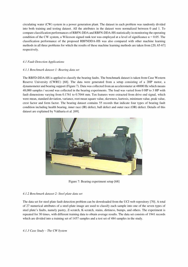
The RBFD-DDA-HS is applied to classify the bearing faults. The benchmark dataset is taken from Case Western

Reserve University (CWRU) [68]. The data were generated from a setup consisting of a 2HP motor, a

dynamometer and bearing support (Figure 7). Data was collected from an accelerometer at 48000 Hz which means

48,000 samples / second was collected in the bearing experiments. The load was varied from 0 HP to 3 HP with

fault dimensions varying from 0.1761 to 0.7044 mm. Ten features were extracted from drive end signal, which

were mean, standard deviation, variance, root mean square value, skewness, kurtosis, minimum value, peak value,

crest factor and form factor. The bearing dataset contains 55 records that indicate four types of bearing fault

condition including health bearing, inner race (IR) defect, ball defect and outer race (OR) defect. Details of this

dataset are explained by Vakharia et al. [69].

Figure 7: Bearing experiment setup [68]

4.1.2 Benchmark dataset 2: Steel plate data set

The data set for steel plate fault detection problem can be downloaded from the UCI web repository [70]. A total

of 27 numerical attributes of a steel-plate image are used to classify each sample into one of the seven types of

steel plate’s faults, namely pastry, Z-scratch, K-scratch, stains, dirtiness, bumps, and others. The experiment is

repeated for 30 times, with different training data to obtain average results. The data set consists of 1941 records

which are divided into a training set of 1457 samples and a test set of 484 samples in the study.

4.1.3 Case Study – The CW System

The proposed RBFN-DDA-HS is applied to perform condition monitoring by learning and classifying a set of real

data collected from a CW system in a power generation plant in Penang, Malaysia. The CW system operates to

provide cooling water continuously to the main turbine condenser to condense steam from the turbine exhaust

[71]. The overall water steam cycle efficiency in power plant is highly relied on the operating condition of the

CW system. Intelligent system such as RBFN-DDA-HS could be helpful to monitor the operating conditions of

the CW system and reduce the frequency of unexpected breakdown. Figure 8 shows an overview of the CW

system. The CW system includes all piping and equipment (such as condensers and drum strainer) between

seawater intake and the outfall where water is returned to the sea. The description of the method of seawater

processing and how it is transferred into the CW system can be referred in [72]. A targeted 80MW power

generation is the fundamental environment to establish the database. For every 5 minutes, an input sample of 12

temperature and pressure measurements was collected at the inlet and outlet points of the condenser. The

operating conditions of the CW system were identified in four classes, which are listed in Table 2. The database

had a total number of 2500 input samples.

Figure 8: The circulating water (CW) system.

Table 2: Operating condition of the CW system

Class Operation Condition

1 Heat transfer in the condenser is efficient and there is no significant

blockage in the piping system

2 Heat transfer in the condenser is not efficient and there is no significant

blockage in the piping system

3 Heat transfer in the condenser is efficient and there is significant blockage

in the piping system

4 Heat transfer in the condenser is not efficient, and there is significant

blockage in the piping system

4.2 Results and Discussion

4.2.1 Performance Comparison between RBFN-DDA and RBFN-DDA-HS

The experiment was conducted by repeatedly training the classifiers using different training and testing data before

computing average classification results. We followed the experimental setup as mentioned in [65], [66] and [20].

In this case, for steel plate [66] problem and CW system case study [20], the experiment was repeated for thirty

and ten times respectively. However, in experiment using the bearing dataset [65] , the number of repetition of

machine learning in training and testing were not mentioned. In our work, we repeat the experiment using RBFN-

DDA and RBFN-DDA-HS for thirty times. All average results of training and testing accuracy of RBFN-DDA

and RBFN-DDA-HS are shown in Table 3. RBFN-DDA-HS performs with higher accuracy rates than RBFN-

DDA in all three dataset. These results signify the performance of RBFN-DDA has been improved after its

learning is integrated with a search and adaptation process by the HS algorithm.

Table 3: Performance comparison between RBFN-DDA and RBFN-DDA-HS

Method

(a) Bearing (b) Steel Plate (c) CW System Case Study

Training

Accuracy

(%)

Testing

Accuracy

(%)

Training

Accuracy

(%)

Testing

Accuracy

(%)

Training

Accuracy (%)

Testing

Accuracy

(%)

RBFN-DDA 65.66 64.35 90.58 68.41 93.16 91.94

RBFN-DDA-HS 80.06 78.81 92.59 69.94 96.56 96.20

A Wilcoxon signed rank test [73] is applied to compare statistically the classification performance between

RBFN-DDA and RBFN-DDA-HS at a level of significance α = 0.05 in all three problems. In this test, the null

hypothesis is that the testing accuracy of RBFN-DDA-HS is the same as that of RBFN-DDA. The alternative

hypothesis is that the testing accuracy of RBFN-DDA-HS is different from RBFN-DDA. By referring to the

results in Table 4, all p-values are smaller than 0.05. This means that the classification performances of RBFN-

DDA and RBFN-DDA-HS in terms of testing accuracy are statistically different. In this regard, RBFN-DDA-HS

achieves better accuracy rates than RBFN-DDA in handling three tasks related to condition monitoring and fault

detection.

Table 4: Results from the Wilcoxon rank tests (at the level of significance α = 0.05)

Dataset p-value

CW System 0.002

Bearing 1.66 X 10-6

Steel Plate 3.86 X 10-6

4.2.2 Performance Comparison with Other Machine Learning Methods

The classification performance of RBFN-DDA-HS is compared with other machine learning methods in all three

problems [65], [66] and [20] from which their accuracy rates are referred. Table 4 shows the results. In bearing

dataset, the result of RBFN-DDA-HS is compared with machine learning classifiers equipped with a feature

selection algorithm (i.e., Random forest and Rotation Forest), and without a feature selection algorithm (i.e., ANN,

SVM, Decision Tree, RBFN-DDA) [65]. The classification accuracy of RBFN-DDA (i.e. 64.35%) is higher than

the classifiers without feature selection such as ANN, SVM and Decision Tree, but is less accurate than classifiers

with feature selection (i.e., Random forest and Rotation Forest). When RBFN-DDA classifier is integrated with

HS, the proposed RBFN-DDA-HS model outperforms all other classifiers by achieving the highest classification

accuracy, i.e., 78.81%.

Next, in steel plate dataset the classification performance of RBFN-DDA-HS is compared with a meta-

heuristic classifier (FAM-GSA) and others single machine learning classifiers (FAM, MLP and RBF) [66]. Based

on the results in Table 4, the testing accuracy of RBFN-DDA is higher than other single machine learning

classifiers. Note that FAM-GSA contributes only a small improvement in testing accuracy, i.e., 0.9% from FAM.

Both FAM-GSA and RBFN-DDA-HS are meta-heuristic classifiers. In comparison, the proposed RBFN-DDA-

HS is more effective than FAM-GSA in detecting steel plat faults. The HS can help improve RBFN-DDA-HS by

a testing accuracy of 2.2% from RBFN-DDA.

The performance of the RBFN-DDA-HS in CW system is compared with fuzzy ARTMAP (FAM) rectangular

basis function network (RecBFN), RBF-based Extreme Learning Machine and RBF-based Constrained

Optimization Extreme Learning Machine (C-ELM). By observing the results in Table 5, the testing accuracy of

RBFN-DDA is the lowest if compared to other machine learning methods. However, when RBFN-DDA is

integrated with the HS algorithm to form the RBFN-DDA-HS, its testing accuracy improves greatly and

outperforms all other machine learning methods. The HS algorithm is effective to search for the optimal parameter

settings.

Table 5: Performance comparison in all three problems

(a) Bearing (b) Steel Plate (c) CW System Case Study

Model

Testing

Accuracy

(%)

Model

Testing

Accuracy

(%)

Model

Testing

Accuracy

(%)

ANN 57.14 FAM 64.84 FAM-RecBFN [20] 95.70

SVM 46.42 FAM-GSA 65.40 ELM (RBF) [67] 94.80

Decision Tree 58.92 MLP 53.50 C-ELM (RBF) [67] 95.89

Random forest 66.07 RBF 59.94 RBFN-DDA 91.94

Rotation Forest 75.00 RBFN-DDA 68.41 RBFN-DDA-HS 96.20

RBFN-DDA 64.35 RBFN-DDA-HS 69.94

RBFN-DDA-HS 78.81

5. Summary

In this study, a hybrid classification model of RBFN-DDA and the HS algorithm is proposed to improve the

RBFN-DDA learning parameters. HS is adopted in the study due to its simplicity, high flexibility and search

efficiency. The effectiveness of the proposed algorithm is demonstrated in the condition monitoring of circulating

water (CW) system and two fault detection benchmark datasets, which are bearing and steel plate. The proposed

RBFN-DDA-HS achieves the highest classification accuracy if compared to other machine learning methods.

Result shows RBFN-DDA-HS can improve classification performance in terms of testing accuracy that has a

range between 2.2% and 22.5% from RBFN-DDA. Besides, the results from the Wilcoxon signed rank test show

that the classification performances of RBFN-DDA and RBFN-DDA-HS are statistically different for all three

condition-monitoring case studies where the latter outperforms the former. HS algorithm is a musical inspired

metaheuristic algorithm. In the future, the classification performances of RBFN-DDA integrated with other types

of metaheuristic algorithm (e.g., from biological, physical or chemical type) would be investigated. In addition,

research may also focus on combining RBFN-DDA with two metaheuristic algorithms. The integration of two

metaheuristic algorithm may explore the search space for optimal solutions more efficiently and effectively.

Acknowledgement

The authors would like to acknowledge the Ministry of Higher Education of Malaysia for the financial support

under the Fundamental Research Grant Scheme (FRGS), Grant No: FP061-2015A and also the Ministry of

Education Malaysia for the financial support under the program myBrain15.

Conflict of Interest: The authors declare that there is no conflict of interests regarding the publication of this

paper.

Reference

1. Stephens, M.P., Productivity and Reliability-Based Maintenance Management. 2010: Purdue University

Press.

2. Waeyenbergh, G. and L. Pintelon, A framework for maintenance concept development. International

Journal of Production Economics, 2002. 77(3): p. 299-313.

3. Blanchard, B.S., Logistics Engineering and Management. 2004: Pearson Prentice Hall.

4. Mohanty, A.R., Machinery Condition Monitoring: Principles and Practices. 2014: CRC Press.

5. Marwala, T. and C.B. Vilakazi, Computational intelligence for condition monitoring. arXiv preprint

arXiv:0705.2604, 2007.

6. Gertler, J., Fault Detection and Diagnosis in Engineering Systems. 1998: Taylor & Francis.

7. Kok, J.N., et al., Artificial intelligence: definition, trends, techniques, and cases. Artificial intelligence,

2009. 1.

8. Ali, Y.H., Artificial Intelligence Application in Machine Condition Monitoring and Fault Diagnosis.

Artificial Intelligence: Emerging Trends and Applications, 2018: p. 275.

9. Tallam, R.M., T.G. Habetler, and R.G. Harley, Stator winding turn-fault detection for closed-loop

induction motor drives. Industry Applications, IEEE Transactions on, 2003. 39(3): p. 720-724.

10. Yao, X., A review of evolutionary artificial neural networks. International journal of intelligent systems,

1993. 8(4): p. 539-567.

11. Singh, G.K. and S.a. Ahmed Saleh Al Kazzaz, Induction machine drive condition monitoring and

diagnostic research—a survey. Electric Power Systems Research, 2003. 64(2): p. 145-158.

12. Lei, Y., et al., Condition monitoring and fault diagnosis of planetary gearboxes: A review. Measurement,

2014. 48: p. 292-305.

13. Isermann, R., Supervision, fault-detection and fault-diagnosis methods — An introduction. Control

Engineering Practice, 1997. 5(5): p. 639-652.

14. Patton, R.J., P.M. Frank, and R.N. Clark, Issues of fault diagnosis for dynamic systems. 2013: Springer

Science & Business Media.

15. Tidriri, K., et al., Bridging data-driven and model-based approaches for process fault diagnosis and

health monitoring: A review of researches and future challenges. Annual Reviews in Control, 2016. 42:

p. 63-81.

16. Miljković, D. Fault detection methods: A literature survey. in 2011 Proceedings of the 34th International

Convention MIPRO. 2011.

17. Ding, S.X., et al., A survey of the application of basic data-driven and model-based methods in process

monitoring and fault diagnosis. IFAC Proceedings Volumes, 2011. 44(1): p. 12380-12388.

18. Venkatasubramanian, V., R. Rengaswamy, and S.N. Kavuri, A review of process fault detection and

diagnosis. Computers & Chemical Engineering, 2003. 27(3): p. 313-326.

19. Venkatasubramanian, V., et al., A review of process fault detection and diagnosis. Computers &

Chemical Engineering, 2003. 27(3): p. 293-311.

20. Tan, S.C., C.P. Lim, and M.V.C. Rao, A hybrid neural network model for rule generation and its

application to process fault detection and diagnosis. Engineering Applications of Artificial Intelligence,

2007. 20(2): p. 203-213.

21. Yin, S., et al., A review on basic data-driven approaches for industrial process monitoring. IEEE

Transactions on Industrial Electronics, 2014. 61(11): p. 6418-6428.

22. Venkatasubramanian, V., et al., A review of process fault detection and diagnosis. Computers &

Chemical Engineering, 2003. 27(3): p. 327-346.

23. Cerrada, M., et al., A review on data-driven fault severity assessment in rolling bearings. Mechanical

Systems and Signal Processing, 2018. 99: p. 169-196.

24. Cocconcelli, M., et al. Diagnostics of ball bearings in varying-speed motors by means of Artificial Neural

Networks. in Proceedings of the 8th International Conference on Condition Monitoring and Machinery

Failure Prevention Technologies. 2011.

25. Muruganatham, B., et al., Roller element bearing fault diagnosis using singular spectrum analysis.

Mechanical Systems and Signal Processing, 2013. 35(1-2): p. 150-166.

26. Ben Ali, J., et al., Application of empirical mode decomposition and artificial neural network for

automatic bearing fault diagnosis based on vibration signals. Applied Acoustics, 2015. 89: p. 16-27.

27. Kankar, P.K., S.C. Sharma, and S.P. Harsha, Vibration-based fault diagnosis of a rotor bearing system

using artificial neural network and support vector machine. International Journal of Modelling,

Identification and Control, 2012. 15(3): p. 185-198.

28. Gunerkar, R.S., A.K. Jalan, and S.U. Belgamwar, Fault diagnosis of rolling element bearing based on

artificial neural network. Journal of Mechanical Science and Technology, 2019. 33(2): p. 505-511.

29. Siddhpura, A. and R. Paurobally, A review of flank wear prediction methods for tool condition

monitoring in a turning process. The International Journal of Advanced Manufacturing Technology,

2013. 65(1-4): p. 371-393.

30. Wang, G., Y. Yang, and Z. Guo, Hybrid learning based Gaussian ARTMAP network for tool condition

monitoring using selected force harmonic features. Sensors and Actuators A: Physical, 2013. 203: p.

394-404.

31. Hesser, D.F. and B. Markert, Tool wear monitoring of a retrofitted CNC milling machine using artificial

neural networks. Manufacturing Letters, 2019. 19: p. 1-4.

32. Xin, Y., Evolving artificial neural networks. Proceedings of the IEEE, 1999. 87(9): p. 1423-1447.

33. Azzini, A. and A.G. Tettamanzi, Evolutionary ANNs: a state of the art survey. Intelligenza Artificiale,

2011. 5(1): p. 19-35.

34. Ding, S., et al., Evolutionary artificial neural networks: a review. Artificial Intelligence Review, 2013.

39(3): p. 251-260.

35. Devikanniga, D., K. Vetrivel, and N. Badrinath. Review of Meta-Heuristic Optimization based Artificial

Neural Networks and its Applications. in Journal of Physics: Conference Series. 2019. IOP Publishing.

36. Bi, T.S., et al. A novel ANN fault diagnosis system for power systems using dual GA loops in ANN

training. in 2000 Power Engineering Society Summer Meeting (Cat. No.00CH37134). 2000.

37. Zaiping, C., et al. Neural network electrical machine faults diagnosis based on multi-population GA. in

2008 IEEE International Joint Conference on Neural Networks (IEEE World Congress on

Computational Intelligence). 2008.

38. Zaranezhad, A., H. Asilian Mahabadi, and M.R. Dehghani, Development of prediction models for repair

and maintenance-related accidents at oil refineries using artificial neural network, fuzzy system, genetic

algorithm, and ant colony optimization algorithm. Process Safety and Environmental Protection, 2019.

131: p. 331-348.

39. Lei, Y., et al., A multidimensional hybrid intelligent method for gear fault diagnosis. Expert Systems

with Applications, 2010. 37(2): p. 1419-1430.

40. Ahmadi, M.A., et al., An accurate model to predict drilling fluid density at wellbore conditions. Egyptian

Journal of Petroleum, 2018. 27(1): p. 1-10.

41. Zhou, H., et al. Effective calculation model of drilling fluids density and ESD for HTHP well while

drilling. in IADC/SPE Asia Pacific Drilling Technology Conference. 2016. Society of Petroleum

Engineers.

42. Sivakumar , M. and R. Parvathi, Application of Neural Network Trained with Metaheuristic Algorithms

on Fault Diagnosis of Muti-level Inverter. Journal of Theoretical & Applied Information Technology,

2014. 61(1).

43. Manjunath, T. and A. Kusagur, Analysis of Different Meta Heuristics Method in Intelligent Fault

Detection of Multilevel Inverter with Photovoltaic Power Generation Source. International Journal of

Power Electronics and Drive Systems, 2018. 9(3): p. 1214.

44. Illias, H.A., X.R. Chai, and A.H. Abu Bakar, Hybrid modified evolutionary particle swarm optimisation-

time varying acceleration coefficient-artificial neural network for power transformer fault diagnosis.

Measurement, 2016. 90: p. 94-102.

45. Xiao, Y. and L. Feng, A novel neural-network approach of analog fault diagnosis based on kernel

discriminant analysis and particle swarm optimization. Applied Soft Computing, 2012. 12(2): p. 904-

920.

46. Shi, H.W., ACO Trained ANN-Based Intelligent Fault Diagnosis. Applied Mechanics and Materials,

2010. 20-23: p. 141-146.

47. Do, Q.H., Predictions of Machine Vibrations Using Artificial Neural Networks Trained by Gravitational

Search Algorithm and Back-Propagation Algorithm. Intelligence, 2017. 15(1): p. 93-111.

48. Zhang, Q., et al., WPD and DE/BBO-RBFNN for solution of rolling bearing fault diagnosis.

Neurocomputing, 2018. 312: p. 27-33.

49. Khilar, P.M. and T. Dash, Multifault diagnosis in WSN using a hybrid metaheuristic trained neural

network. Digital Communications and Networks, 2020. 6(1): p. 86-100.

50. Liu, Y., et al. Training radial basis function networks with particle swarms. in International Symposium

on Neural Networks. 2004. Springer.

51. Hudak, M.J., Rce classifiers: Theory and practice. Cybernetics and System, 1992. 23(5): p. 483-515.

52. Berthold, M.R. and J. Diamond, Constructive training of probabilistic neural networks.

Neurocomputing, 1998. 19(1): p. 167-183.

53. Robnik-Šikonja, M., Data generators for learning systems based on RBF networks. IEEE transactions

on neural networks and learning systems, 2016. 27(5): p. 926-938.

54. Geem, Z.W., J.H. Kim, and G. Loganathan, A new heuristic optimization algorithm: harmony search.

Simulation, 2001. 76(2): p. 60-68.

55. Lee, K.S., et al., The harmony search heuristic algorithm for discrete structural optimization.

Engineering Optimization, 2005. 37(7): p. 663-684.

56. Karayiannis, N.B., Reformulated radial basis neural networks trained by gradient descent. IEEE

Transactions on Neural Networks, 1999. 10(3): p. 657-671.

57. Simon, D., Training radial basis neural networks with the extended Kalman filter. Neurocomputing,

2002. 48(1): p. 455-475.

58. Kurban, T. and E. Beşdok, A comparison of RBF neural network training algorithms for inertial sensor

based terrain classification. Sensors, 2009. 9(8): p. 6312-6329.

59. Barreto, A.M., H.J. Barbosa, and N.F. Ebecken. Growing compact RBF networks using a genetic

algorithm. in Neural Networks, 2002. SBRN 2002. Proceedings. VII Brazilian Symposium on. 2002.

IEEE.

60. Hamadneh, N., et al., Learning logic programming in radial basis function network via genetic

algorithm. Journal of Applied Sciences(Faisalabad), 2012. 12(9): p. 840-847.

61. de Castro, L.N. and F.J. Von Zuben. An immunological approach to initialize centers of radial basis

function neural networks. in Proc. of CBRN’01 (Brazilian Conference on Neural Networks). 2001.

62. Yu, B. and X. He. Training radial basis function networks with differential evolution. in In Proceedings

of IEEE International Conference on Granular Computing. 2006. Citeseer.

63. Horng, M.-H., et al., Firefly meta-heuristic algorithm for training the radial basis function network for

data classification and disease diagnosis. 2012: INTECH Open Access Publisher.

64. Mahdavi, M., M. Fesanghary, and E. Damangir, An improved harmony search algorithm for solving

optimization problems. Applied Mathematics and Computation, 2007. 188(2): p. 1567-1579.

65. Kavathekar, S., N. Upadhyay, and P. Kankar, Fault classification of ball bearing by rotation forest

technique. Procedia Technology, 2016. 23: p. 187-192.

66. Tan, S.C. and C.P. Lim, Evolving an adaptive artificial neural network with a gravitational search

algorithm, in Intelligent Decision Technologies. 2015, Springer. p. 599-609.

67. Wong, S.Y., Novel Extreme Learning Machines For Pattern Classification, Data Regression, And Rules

Generation, in College Of Engineering2015, Universiti Tenaga Nasional: Malaysia.

68. Loparo, K.A., Bearing vibration data set.

69. Vakharia, V., V.K. Gupta, and P.K. Kankar, A comparison of feature ranking techniques for fault

diagnosis of ball bearing. Soft Comput., 2016. 20(4): p. 1601-1619.

70. Lichman, M., UCI Machine Learning Repository, 2013, University of California, Irvine, School of

Information and Computer Sciences.

71. Tenaga Nasional Berhad, System description and operating procedures, 1999: Prai Power Station Stage

3.

72. Tan, S.C. and C.P. Lim, Application of an adaptive neural network with symbolic rule extraction to fault

detection and diagnosis in a power generation plant. IEEE Transactions on Energy Conversion, 2004.

19(2): p. 369-377.

73. Woolson, R., Wilcoxon signed‐rank test. Wiley encyclopedia of clinical trials, 2007: p. 1-3.

Figures

Figure 1

Overview of condition monitoring and fault detection approaches

Figure 2

The DDA algorithm with two thresholds

Figure 3

The structure of RBFN-DDA [53]

Figure 4

RBFN-DDA Training for one epoch

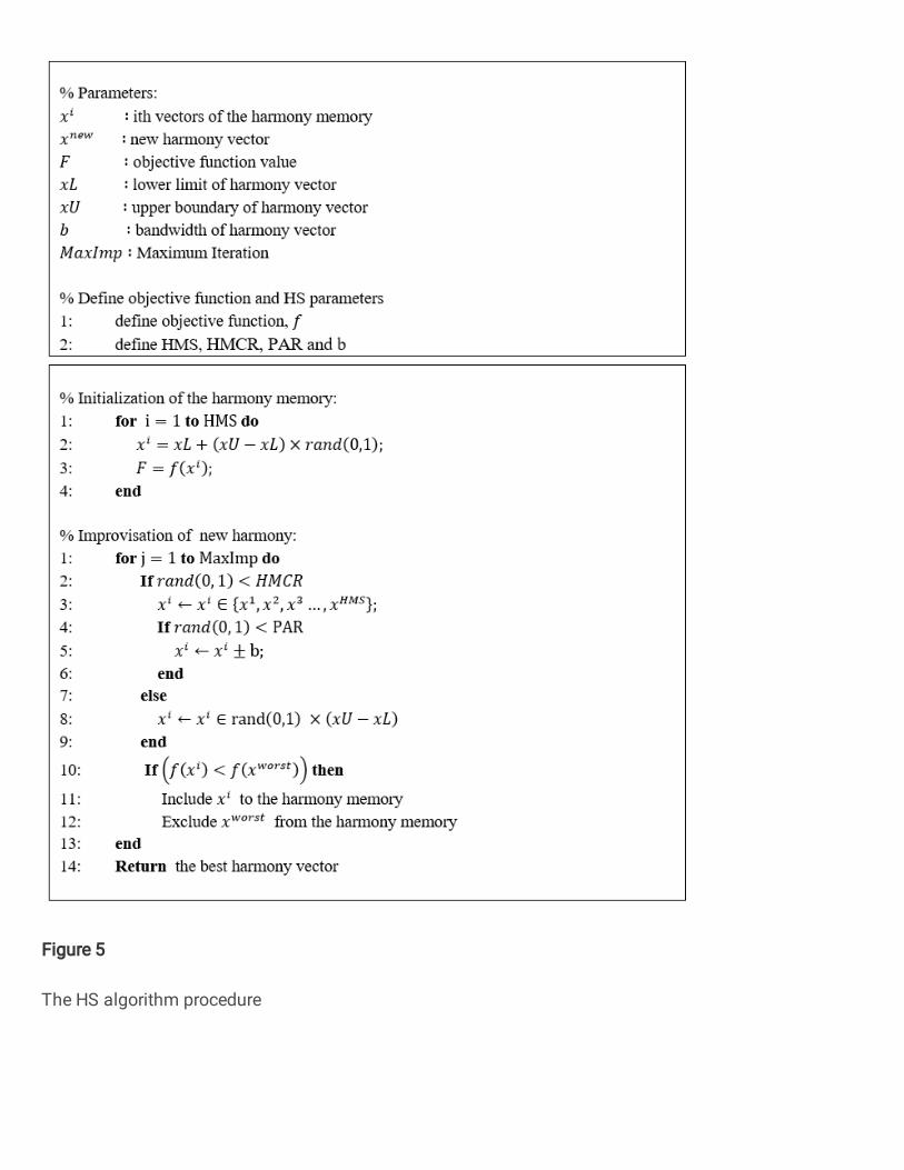
Figure 5

The HS algorithm procedure

Figure 6

The �ow chart of creating an RBFN-DDA-HS model

Figure 7

Bearing experiment setup [68]

Figure 8

The circulating water (CW) system.