Human Capital and Elimination of Rural Poverty: A Case ...kurosaki/ids1999r.pdf · From descriptive...

Human Capital and Elimination of Rural Poverty:A Case Study of

the North-West Frontier Province, Pakistan ∗

Takashi KUROSAKI † and Humayun KHAN ‡

January 2001

Abstract

In this paper, we analyze the interaction of poverty, risk, and human capital atthe household level, in order to obtain insights to an important development issue ofeliminating rural poverty in developing countries. In the recent literature, the potentialof human capital in overcoming two symptoms of poverty—low income and vulnerabilityto income risk—is drawing attention. As an attempt to extend this line of research,we implemented an original, detailed household survey in 1999/2000 in the North-WestFrontier Province, Pakistan. This case study represents a rural region with an adverseland-man ratio and low human development. The 1999/2000 survey was designed as are-survey of households that were investigated in 1996/97, so that we can examine thedynamics of poverty.

From descriptive analysis based on the 1999/2000 survey, it is suggested that, inthe sample villages, human capital, especially education, plays an important role inovercoming the two symptoms of poverty through expanded opportunities of non-farmemployment. Another important implication is that the lack of mechanisms to copewith income risk is likely to result in low accumulation of human capital. A policyimplication of these findings is that provision of primary education and primary healthcare and public interventions to reduce the cost of income risk such as employmentguarantee schemes may yield a large social benefit in the long run.

∗The authors are grateful to the Ministry of Foreign Affairs, Japan, for funding the principal part of thisproject through the FASID’s development research facility 1999/2000. Funding assistance from Seimei-Kai,Tokyo-Mitsubishi Bank, was also used, to which the authors express their gratitude. The views reflected inthis paper, however, are solely the authors’ own and should not be taken to represent any of their sponsors.†Institute of Economic Research, Hitotsubashi University, 2-1 Naka, Kunitachi, Tokyo 186-8603 Japan.

Phone: 81-42-580-8363; Fax: 81-42-580-8333; E-mail: [email protected].‡Institute of Development Studies, N.W.F.P. Agricultural University, Peshawar, Pakistan.

Human Capital and Elimination of Rural Poverty:

A Case Study of the North-West Frontier Province, Pakistan

1 Introduction

Eliminating rural poverty in developing countries remains an important development issue

(World Bank 2000). To understand poverty in developing countries, it is imperative to pay

sufficient attention to the microeconomic mechanism of poverty, such as how a household has

been fallen into poverty, how it will react to changes in external environments including public

policies, and how aggregate measures of poverty will change after households’ reaction. This

paper addresses this issue by analyzing the interaction of poverty, risk, and human capital

at the household level. Key emphasis is laid on the potential of human capital in overcoming

two symptoms of poverty—low income and vulnerability to income risk.

In this paper, we analyze the interaction in a descriptive way using micro household data

collected from rural areas in the North-West Frontier Province (NWFP), Pakistan. We im-

plemented an original household survey in the fiscal year of 1999/20001 in NWFP to collect

detailed information on household demography, consumption, income, production, assets,

and social relations. The study area represents a case with an adverse land-man ratio and

low human development. A distinctive feature of this survey is that we re-surveyed house-

holds that were investigated in 1996/97 (Kurosaki and Hussain 1999). The intertemporal

dimension of the two period panel data enables us to examine the dynamics of poverty.

The motivation of this study is the same as the one adopted in the 1996/97 survey

(Kurosaki and Hussain 1999, pp.3-4). Among important assets whose lack characterizes

poverty, such as land, livestock, financial assets, human capital, etc, our attention is fo-

cused on improving human capital and increasing non-farm income since they are key to the

enhancement of welfare positions of the rural poor in the study region.

Non-farm income and enhanced human capital are linked through the individual motiva-

tion of investment in human capital. When farmers decide to send their children to schools,

they are usually motivated by the desire of finding non-farm, lucrative jobs for their chil-

dren. As a result, investment in human capital in rural areas is likely to be closely related

with non-farm activities and higher economic returns there (Lanjouw 1999; Fafchamps and

Quisumbing 1999; Kurosaki 2000). This phenomenon may lead to diversification of a rural

1The fiscal year of “1999/2000” refers to a period from July 1999 to June 2000.

1

economy. At the same time, in developing countries, it is likely that individual decisions

with respect to job choices are jointly decided at the household level and households’ ability

to smooth consumption might become an important determinant of the diversification of a

household economy (Kurosaki 1998; 2000).

With these issues in mind, we carried out in 1999/2000 a re-survey of sample villages

and sample households that were investigated in 1996/97. The field survey was designed to

obtain insights to this broad issue by sampling three villages that were in sharp contrast

with respect to the stage of development. This paper is prepared as one of the final reports

for the re-survey. Although only two names of the principal authors are on the front page,

we regard this paper as the joint product of all those involved in the project (see Appendix

2 for the full list of project participants).

In the followings, sample villages and sample households are described in Section 2,

with special emphasis on transitions that have happened since the first survey. In Section 3,

household data are analyzed in a descriptive way. Measures of concern are consumption level,

poverty indices, human capital indicators, income sources, labor force allocation, and risk-

coping ability including the use of credit markets. In Section 4, the findings are summarized

with discussion on their policy implications. Details of the household survey and the data

set are given in Appendix.

2 Sample Villages and Sample Households

2.1 NWFP Economy and Poverty Indicators

NWFP is geographically the smallest province among the four provinces in Pakistan, ac-

counting for about 9% of total area and 13% of total population.2 Compared with Punjab,

which is the center of agriculture and related industries, and Sind, where a metropolitan city

of Karachi is located, NWFP could be characterized as an economically backward province.

The share of manufacturing industries in labor force in the province is much smaller than

those in Punjab and Sind. Electricity consumption per capita was only half the level enjoyed

in Punjab and Sind. NWFP’s economy is more dependent on service sectors and remittances

than on commodity sectors including agriculture and manufacturing industries.

In Table 2-1, regional disparity in Pakistan is shown in terms of the World Bank’s es-

timates for consumption poverty measures. It is robustly found regardless of data sources

2These numbers do not include the Federally Administered Tribal Areas on the Afghan border. All thesample villages are in non-tribal, settled areas of the province.

2

that poverty incidence (headcount index: HCI) is higher in rural areas than in urban areas

and that urban Sind has the lowest HCI. On the other hand, the ranking among rural re-

gions, especially the relative ranking of rural NWFP, differs depending on the choice of data

sources. Based on the Pakistan Integrated Household Survey (PIHS) 1991, rural NWFP has

the lowest incidence of poverty among rural areas in Pakistan at around 21%. Based on the

Household Income and Expenditure Survey (HIES) 1990/91, HCI of rural NWFP is 41%,

which is higher than the national average.

Our impression from the field suggests that the real picture is in between. In a relative

sense, HCI of rural NWFP might be lower than those of rural areas of other provinces but

not to the extent shown by the PIHS 1991 data. On the other hand, poverty measures

in Pakistan are sensitive to adjustments for scale economy of household size (Lanjouw and

Ravallion 1995). Since extended family system is common in NWFP and the World Bank’s

estimates do not take into account of the scale economy, the poverty incidence in Table 2-1

might be overestimated for rural NWFP.

In any case, the absolute size of HCI (about 21 to 41 % of people are below the poverty

line in rural NWFP) might be sufficient to justify our locational choice for poverty inves-

tigation. Furthermore, as shown below, the living standards in rural NWFP are likely to

be overvalued if income/consumption measures are used, ignoring the region’s backwardness

in human development. This disparity, i.e., income/consumption poverty is less than hu-

man development poverty, is a notorious characteristic of Pakistan’s economy, to which late

Dr. Mahbubul Haq drew attention in the Human Development Reports. We focus on rural

NWFP because this is the region where this disparity applies the most.

Region-wise human development indicators are shown in Table 2-2. According to PIHS

1991, literacy rates in NWFP were lower than Sind and Punjab. Female literacy rates were

especially low. This phenomenon is related with the prevalence of purdah (social segregation

of women) in the province. NWFP is lagging behind Punjab and Sind in infant mortality

rates also. To examine the robustness, Table 2-3 shows literacy rates estimated from national

census. In 1998, male literacy rate (15 years and older) in NWFP was 51% in contrast to

Punjab’s 57% and Sind’s 56%. For females, the disparity widens: only 17% in NWFP were

literate whereas 31% in Punjab and 33% in Sind were able to read. However, in comparison

with 1981 figures, literacy rates in 1998 have improved substantially in NWFP.

3

2.2 Objectives of the 1999/2000 Survey

The data set used in this paper was compiled from a household sample survey carried out

in three villages in Peshawar District, NWFP, in 1999/2000 as a joint research project (see

Appendix 2). The study area represents a case with an adverse land-man ratio and low

human development.

In 1996/97, we implemented a sample survey with similar motivations. From cross-section

analyses based on the 1996/97 data, we found that development status of the three villages

(income/consumption level and irrigation level), accumulation of human capital (education,

health, labor force), and labor allocation patterns (job diversification, non-farm employment,

household self-employment, etc.) are closely related. The relationship was consistent with

our hypothesis that human capital and non-farm employment are key to the eradication

of rural poverty in an area with an adverse land-man ratio (Kurosaki and Hussain 1999,

pp.22-23).

Strictly speaking, however, it is possible that the empirical findings above were deter-

mined solely by fixed effects of villages and households. In other words, the relations above

could be spurious and imply no structural relationship among human capital, poverty, and

labor allocation. To refute this argument, we need to control fixed effects of villages and

households. For this purpose, we re-surveyed in 1999/2000 households that were investigated

in 1996/97. The intertemporal dimension of the two period panel data enables us not only

to control fixed effects in an econometric sense but also (and more importantly) to examine

the dynamics of poverty.

To summarize, the main objective of this survey was to collect dynamic information

about household economy with respect to demography, labor force, education, agricultural

production, non-agricultural production, household income and consumption, assets, and

social relations. The scope of the survey would enable us to examine the dynamics of poverty

in a multidimensional way. The multidimensional nature of poverty has been emphasized in

the recent literature also (World Bank 2000).

2.3 Survey Design

In choosing sample villages in 1996, we put three major conditions that, first, the village

size be the same in terms of total population and number of households, second, the selected

villages have similar ways of handling their social, political, cultural and economic problems

and they have the same language and ethnic background, and, third, tenancy structure be

4

the same. At the same time, to ensure that the cross section data thus generated would

provide dynamic implications, we carefully chose villages with different levels of economic

development. The first criterion was agricultural technology. One of the three sample vil-

lages would be rain-fed (barani), another semi-irrigated, while the other as fully-irrigated.

Another criterion was that the selected villages be located along the rural-urban continuum

so that it would be possible to decipher the subsistence versus market orientation of farming

communities in the project area.

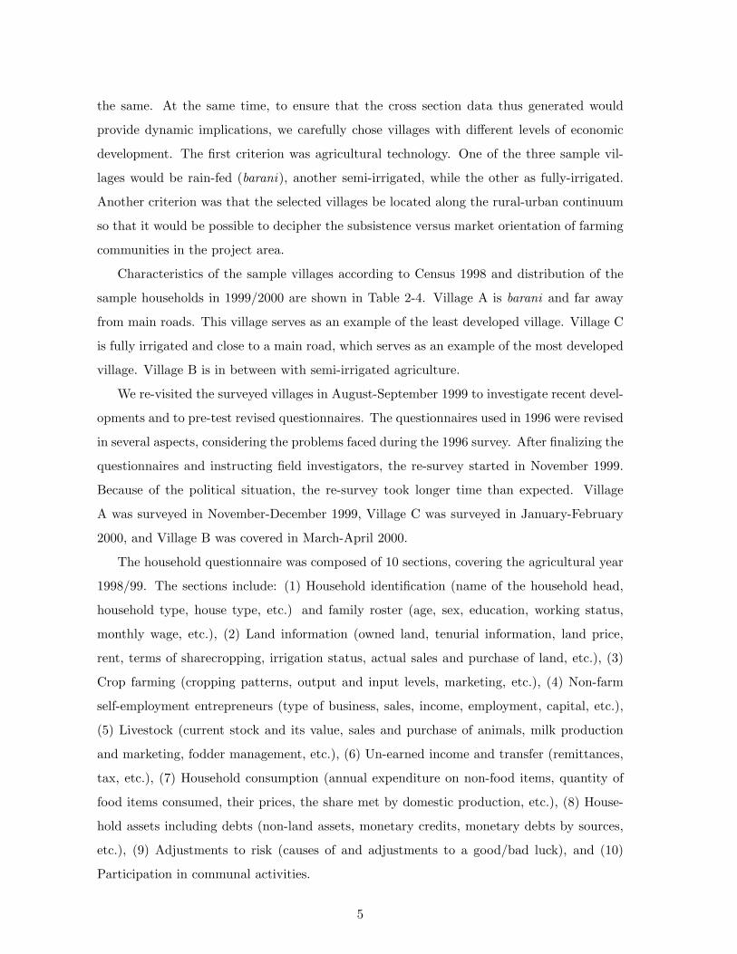
Characteristics of the sample villages according to Census 1998 and distribution of the

sample households in 1999/2000 are shown in Table 2-4. Village A is barani and far away

from main roads. This village serves as an example of the least developed village. Village C

is fully irrigated and close to a main road, which serves as an example of the most developed

village. Village B is in between with semi-irrigated agriculture.

We re-visited the surveyed villages in August-September 1999 to investigate recent devel-

opments and to pre-test revised questionnaires. The questionnaires used in 1996 were revised

in several aspects, considering the problems faced during the 1996 survey. After finalizing the

questionnaires and instructing field investigators, the re-survey started in November 1999.

Because of the political situation, the re-survey took longer time than expected. Village

A was surveyed in November-December 1999, Village C was surveyed in January-February

2000, and Village B was covered in March-April 2000.

The household questionnaire was composed of 10 sections, covering the agricultural year

1998/99. The sections include: (1) Household identification (name of the household head,

household type, house type, etc.) and family roster (age, sex, education, working status,

monthly wage, etc.), (2) Land information (owned land, tenurial information, land price,

rent, terms of sharecropping, irrigation status, actual sales and purchase of land, etc.), (3)

Crop farming (cropping patterns, output and input levels, marketing, etc.), (4) Non-farm

self-employment entrepreneurs (type of business, sales, income, employment, capital, etc.),

(5) Livestock (current stock and its value, sales and purchase of animals, milk production

and marketing, fodder management, etc.), (6) Un-earned income and transfer (remittances,

tax, etc.), (7) Household consumption (annual expenditure on non-food items, quantity of

food items consumed, their prices, the share met by domestic production, etc.), (8) House-

hold assets including debts (non-land assets, monetary credits, monetary debts by sources,

etc.), (9) Adjustments to risk (causes of and adjustments to a good/bad luck), and (10)

Participation in communal activities.

5

As is examined in more detail below, we could not re-survey some of the sample house-

holds covered in 1996/97. In such a case, we replaced them by new samples so that the total

sample size in 1999/2000 be comparable to the size in 1996/97. Replacement samples were

chosen from the same household category (owner farm, owner-cum-tenant farm, pure tenant

farm, and non-farm households). The final sample size in 1999/2000 is comparable to that

in 1996/97 (Table 2-4).

2.4 Changes in the Study Villages

Summary of village questionnaires is given in Table 2-5. Radical changes have not been

observed in the villages since 1996. Several developments in social infrastructure are worth

noting, however.

Like other parts of NWFP, political awareness among the people in the surveyed villages

has increased. Now they ask for their rights. For example during the survey, even the

illiterate people of Village A stressed for their demand to appear in the press, so that the

government come forward to take direct action against the concerned departments. They

were logging complaints about the irregularities in the supply of drinking water and the

shortage of female teaching staff in the school.

Village A, which is close to the tribal areas, is very conservative. The poor infrastructure

of this village has restricted mobility of female children to go to school located away from

the village. Similarly, it is also very difficult for female teachers to come for duty from

other villages of NWFP. This problem restricts the female literacy in the area. The village

community is willing to offer the services of their educated females to be appointed as teacher

at the village female school. The change in the attitude of the people toward female education

and female employment is a promising sign for development in Village A, although it has

not yet changed the overall situation of female education (see Section 3.2). The number of

schools has increased in Village C as well.

The telephone connection facility to Village A is another development worth mentioning.

Although at the time of the survey only one household had a telephone connection, very

soon other people will install a telephone at their house, keeping in view the race in mind

among the village elite for acquiring such facility. Even this single telephone is benefiting a

number of other people in the village. In the rural set-up of NWFP, it is common to receive

messages for other households. Village people working abroad can also use this connection

to pass on their messages to their families or to call their family members and talk on this

6

telephone.

A new institution called “Village Welfare Committee” for resolving local disputes has

been established and becoming popular in Village B. It is replacing the traditional system

of jirga, in which only the elite of the locality were eligible for becoming a member. In this

committee, people voluntarily offer their money, services, and time to resolve disputes at the

village level.

Nursery raising and home making of squashes for markets are considered profitable busi-

nesses in Village C. The number of nurseries has considerably increased and making of

squashes has also become popular in this village.

The long awaited demand of the people in Village C, i.e. the connection of gas supply, has

been fulfilled. The gas, which is comparatively cheaper than firewood, will further develop

the village. Resources that were previously spent on firewood purchase are now spent on

other consumption items, such as health, education, etc. It also helps protect the village

environment.

The common changes that have taken place in all the three villages are as follows:

1. The off-farm business, mainly opening of general shops, has slightly developed.

2. Due to improvement in public transport facility, mobility of people has increased.

3. More agricultural land has been converted into residential areas.

During the three years since the first survey, Pakistan’s economy suffered from macroe-

conomic stagnation. The GDP growth rate wwas slowed down; the inflation rates went up,

especially the prices of essential items. Reflecting this macroeconomic situation, the general

living standard has not improved substantially in the study villages. On the other hand,

when households are hit by a bad luck that is sufficiently severe, a few of them decide to

leave the village; others continue to stay home, sending their working males to urban cities

including those abroad for job. When this happened to some of the 1996 surveyed house-

holds, it became difficult for us to re-survey them during the 1999/2000 survey. Therefore,

before going into the analysis of household data, let us discuss the success rate of re-surveys

and the household level transition.

2.5 Household Transition between the Two Surveys

In Table 2-6, the transition of the sample households is shown for each village. Households

are classified into four types depending on their tenancy status. “Owner Farm Households”

7

are households who operate agricultural land owned by themselves. If farm households

operate both owned and rented land, they are classified as “Owner-cum-Tenant (OCT)

Farm Households.” “Pure Tenant Farm Households” are those who do not own land but

rent in land for cultivation purpose. We define “Non-Farm Households” as those who do

not at all cultivate agricultural land. Therefore, this category includes some households

who are dependent on agriculture-related income sources, such as agricultural wage labor,

animal husbandry, or land rents, as long as they do not operate any farm land. However, the

number of such households is negligible, because the majority of agricultural wage laborer

households, shepherd households, and landlord households either operate some land or earn

their major portion of their income from non-agricultural sources.

A household that was surveyed in 1996 should belong to one of these four categories.

In the 1999/2000 survey, either we were able to re-survey it as a household that belongs to

one of these four categories or unable to re-survey it (“n.a.” in the table). If a household

is re-surveyed and has not changed its tenancy status, it is recorded on the diagonal of

a transition matrix. By analyzing the distribution of sample households in the transition

matrix, we can obtain inferences on social mobility in the study region. If the village society

is highly mobile, the percentage of “off-diagonal” samples is high.

Table 2-6A for a rain-fed, less-developed village (Village A) is more complicated than

those for Villages B and C. This is because two large households surveyed in 1996 were

divided into three households each and all the six households were surveyed in 1999. A

typical joint family used to live together, with a household head owning their family land,

sharing kitchen and household income. Married sons live together with the household head

along with their wives and children. In our survey, such a case is counted as one household.

When the household head dies or becomes older, the land may be distributed among sons,

who start to live separately on that occasion. In our survey when we encounter such cases,

each family of each son is counted as one household. Because of this kind of household

division, two households surveyed in 1996 were re-surveyed in 1999 as six households.

In Village A, 91 out of 117 households surveyed in 1999 are traceable to the 1996 survey

(Table 2-6A, panel “a”). To see it in a reverse way, 87 out of 119 households surveyed in 1996

were re-surveyed in 1999 (Table 2-6A, panel “b”). The re-survey success rate is substantially

lower than the other two villages, because migration of a whole household or all the male

adults is more frequent in Village A than in the other villages.

Transition probabilities of these 87 households are shown in the last rows of Table 2-6A.

8

The off-diagonal percentage of “Owner Farm Households” is relatively low at 32%. This is as

expected since this is likely to be the class with the highest social stability. The off-diagonal

percentage of “Non-Farm Households” is also relatively low at 28%.

In sharp contrast, “OCT Farm Households” and “Pure Tenant Households” have higher

probability of changing their status—the former is likely to change its status into “Owner

Farm Households,” whereas the latter tends to shift to the status of “Non-Farm Households.”

The pattern of OCT farms could be explained by two different tenancy adjustments—when

tenant agriculture becomes lucrative, an OCT farm household might purchase the land under

tenancy to become a owner farm household; when tenant agriculture becomes economically

unattractive, an OCT farm household might give the land under tenancy back to its owner

so that the household becomes a owner farm household. The high mobility of pure tenant

households into non-farm households suggests that it is more likely that they would give up

farming quickly when tenant agriculture becomes economically unattractive. The important

point is that the transition patterns indicate that the four household categories can be

grouped into two: the landed group (owner farm and OCT farm households) and the landless

group (pure tenant farm and non-farm households).

In more irrigated villages, the incidence of migration is less frequent than in the rain-

fed village. In Village B, 111 out of 116 households surveyed in 1996 were re-surveyed in

1999/2000 (Table 2-6B); in Village C, 107 out of 120 households surveyed in 1996 were re-

surveyed in 1999/2000 (Table 2-6C). The failure ratio of re-survey is slightly higher in Village

C than in Village B because several households in Village C, a more urbanized village, have

shifted their life base into the city and have become less cooperative to the village survey.

The overall pattern in the two villages is similar to that in Village A. Non-farm house-

holds, followed by owner farm households, tend to remain in the same category; the mobility

between owner and OCT farm households is relatively high; and the mobility between pure

tenant farm and non-farm households is also high. One difference is that the transition

probability for non-farm households to become farm households (off-diagonal probability for

non-farm households) is low at around 13%, which is approximately the half of the transition

probability in Village A. In other words, the transition from farm households into non-farm

households is more irreversible in the irrigated villages than in the rain-fed, traditional vil-

lage.

9

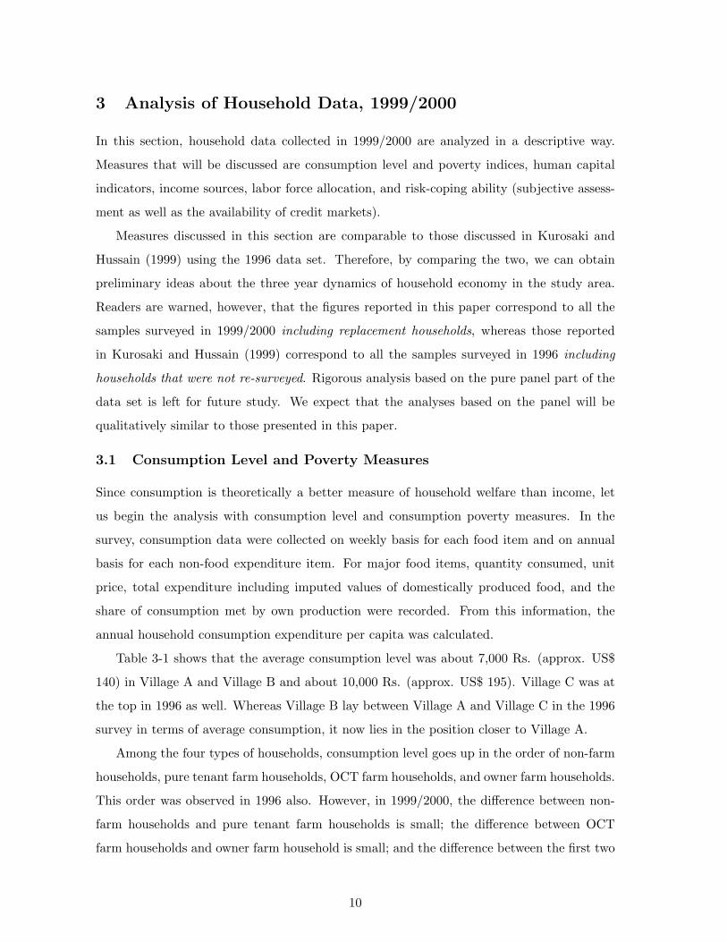
3 Analysis of Household Data, 1999/2000

In this section, household data collected in 1999/2000 are analyzed in a descriptive way.

Measures that will be discussed are consumption level and poverty indices, human capital

indicators, income sources, labor force allocation, and risk-coping ability (subjective assess-

ment as well as the availability of credit markets).

Measures discussed in this section are comparable to those discussed in Kurosaki and

Hussain (1999) using the 1996 data set. Therefore, by comparing the two, we can obtain

preliminary ideas about the three year dynamics of household economy in the study area.

Readers are warned, however, that the figures reported in this paper correspond to all the

samples surveyed in 1999/2000 including replacement households, whereas those reported

in Kurosaki and Hussain (1999) correspond to all the samples surveyed in 1996 including

households that were not re-surveyed. Rigorous analysis based on the pure panel part of the

data set is left for future study. We expect that the analyses based on the panel will be

qualitatively similar to those presented in this paper.

3.1 Consumption Level and Poverty Measures

Since consumption is theoretically a better measure of household welfare than income, let

us begin the analysis with consumption level and consumption poverty measures. In the

survey, consumption data were collected on weekly basis for each food item and on annual

basis for each non-food expenditure item. For major food items, quantity consumed, unit

price, total expenditure including imputed values of domestically produced food, and the

share of consumption met by own production were recorded. From this information, the

annual household consumption expenditure per capita was calculated.

Table 3-1 shows that the average consumption level was about 7,000 Rs. (approx. US$

140) in Village A and Village B and about 10,000 Rs. (approx. US$ 195). Village C was at

the top in 1996 as well. Whereas Village B lay between Village A and Village C in the 1996

survey in terms of average consumption, it now lies in the position closer to Village A.

Among the four types of households, consumption level goes up in the order of non-farm

households, pure tenant farm households, OCT farm households, and owner farm households.

This order was observed in 1996 also. However, in 1999/2000, the difference between non-

farm households and pure tenant farm households is small; the difference between OCT

farm households and owner farm household is small; and the difference between the first two

10

(landless) and the last two (landed) is large. In other words, during the last three years,

landed households did better than the landless. Considering the macroeconomic stagnation

during the period, this observation can be interpreted as the reflection of a decline of returns

to labor (the dominant asset for the landless) relative to returns to land (the dominant asset

for the landed). Agricultural land has a natural hedge function against inflation whereas

un-skilled labor is vulnerable to macroeconomic stagnation and inflation.

Foster-Greer-Thorbecke (FGT) poverty measures were calculated for our sample in 1999/2000

(Foster, Greer, and Thorbecke 1984), with the poverty line at 7,140 Rs. per capita deflated

using rural CPI.3 The FGT measure is defines as:

P (α) =1n

q∑i=1

(z − yiz

)α, (1)

where α is a parameter of the FGT measures, n is the number of individuals, q is the number

of individuals below the poverty line z, and yi is per-capita consumption of individual i which

is below the poverty line.

The expression in equation (1) should be modified when we apply it to our data set where

per-capita consumption is calculated at the household level, which yields

P (α) =1N

Q∑h=1

wh

(z − yhz

)α, (2)

where N is the number of households, Q is the number of households below the poverty line,

wh is household h’s weight defined as nh/n, where nh is the household size of h and n is the

average household size, and yh is per-capita consumption of household h which is below the

poverty line.4

When α = 0, the FGT measure becomes headcount index (HCI), which was estimated

at 87% in Village A, 91% in Village B, and 70% in Village C (Table 3-1). These numbers

are higher than the ratio of households in poverty because larger households are more likely

to be below the poverty line in our case.5 When α = 1, the measure becomes poverty gap

3The figure of 7,140 Rs. for 1996 was obtained from Lanjouw (1996) who estimated poverty lines from1991 Pakistan Integrated Household Survey, using the basic-needs-food-expenditure method. See also WorldBank (1995) for more discussion on poverty lines in Pakistan.

4In Kurosaki and Hussain (1999), we wrongly treat i in equation (1) as a household and n is the numberof households. Since FGT measures are usually defined at the individual level to obtain meaningful povertymeasures, we adopt the standard definition in this paper.

5Our measures of per-capita consumption is a simple division of household consumption by the householdsize. Therefore, we have not taken account of the scale economy of household size. As Lanjouw and Raval-lion (1995) demonstrated, the positive correlation between household size and poverty measures might be a

11

ratio (PGR), estimated at 0.37 (Village A), 0.34 (Village B), and 0.19 (Village C). Squared

poverty gap ratio (SPGR) with α = 2 was estimated at 0.18 (Village A), 0.15 (Village B),

and 0.07 (Village C).

All the poverty measures in Table 3-1 are the lowest in Village C, a fully-irrigated, well-

developed village. This is the same as in 1996 shown in Table 3-2, which is a corrected

version for Kurosaki and Hussain (1999, Table 2). In 1996, Village B had lower poverty

measures than Village A but the difference disappears in 1999/2000—the order of Village A

and Village B changes depending on the choice of poverty measures.

Among household categories, in all the three villages, non-farm and pure tenant house-

holds have higher poverty measures than owner farm and OCT farm households in 1999/2000

(Table 3-1). Here again the disparity between the landed and the landless appears clearly.

Let us compare two tables over time (Table 3-1 and Table 3-2). First, the level of poverty

measures have not changed much over the three year period. In Village A, poverty measures

remain the same, whereas in Village B, most of the measures have worsened. In Village C,

poverty incidence (P (0)) remains the same while poverty depth (P (1)) and poverty severity

(P (2)) have been improved. These patterns are consistent with the authors’ impression in

the field. Especially, a decrease in the ultrapoverty reflected in the reduced value of P (2)

in Village C is worth mentioning. At the same time, relative deprivation of Village B is a

worrying sign.

Second, the disparity between the landed and the landless has become more apparent

after three years. From poverty measures also, it has been demonstrated that landless

households are more vulnerable to macroeconomic stagnation than landed households.

Considering a possibility that the consumption data could be underestimates due to the

omission of less frequently consumed items, a more robust method of stochastic dominance

was applied to the 1999/2000 data also. Results (not shown here) have robustly supported

the pattern discussed above.

To summarize, in the study area, a clear disparity in welfare (both the level in a static

framework and the vulnerability in a dynamic framework) exists depending on the economic

development level of each village and the asset position of each household. In the following

subsections, we investigate how this profile is related with other variables of concern, namely,

human capital, occupational structure, and risk.

spurious product from ignoring the scale economy. It is left for further research to explore this issue for oursample.

12

3.2 Human Capital

As a measure of human capital, we tabulate household size, labor force size, adult literacy

rates, and school enrollment of children. The total number of 3,267 individuals are included

in 352 sample households—the average household size is therefore 9.3, which is the same

as in 1996. This size is not only very large by international standard but also larger than

the national average in Pakistan. Prevalence of extended family system is reflected in this

number.

Table 3-3 shows demographic information by village and by household category. Farm

households are generally larger than non-farm households and households in rain-fed Village

A are generally larger than those in irrigated villages (B and C). This is the same as in

1996. A possible reason for the large household size in Village A is that labor markets in

rain-fed areas are of casual character and hence risky. We can interpret the large size of

a household as a reflection of household strategy to diversify risk or to share risk within

an extended family. Farm households tend to be larger because they can support more

household members through domestic food supply and because family labor is likely to be

more efficient than hired labor in farming so that there is a gain in having more family

workers within a household.

The total number of male members in the sample is 1,687, much larger than that of

female members (1,580). The female-male ratio from our data is 0.937, which is slightly

higher than we observe in 1996 (0.918) but still very low by international standard. Since

NWFP’s economy depends on remittances which are sent by men, a figure higher than the

national average is reasonable. A point to remark is that the low female/male ratio could

be interpreted as a consequence of gender biases against females (Dreze and Sen 1989).

In the survey, individual attributes are recorded in detail, including their age, sex, edu-

cation, working status, monthly wage, etc. The average size of working male members is 2.5

in Village A, 2.0 in Village B, and 2.2 in Village C. The difference is smaller than the case for

the household size. This is because households in Village A send more family members as a

temporary migrant worker than in other villages. Therefore, the ratio of male labor force in

the village household is smaller than in the other two villages.6 Literacy rates of the working

male members are the highest in Village C at 62%, followed by 45% in Village A and 32%

6Note that migrant workers are not defined as household members in this project. However, since theycomprise an indispensable part of the household economy, all individual attributes of these family membersare recorded in the survey in the same format as that for household members in the village (see demographyfiles in Appendix 1).

13

in Village B (Table 3-3). Among the four household categories, owner farm households have

the highest literacy rates among the working male. These patterns are similar to what we

found in 1996 (Kurosaki and Hussain 1999).

Information on working female population is also given in the table. The category of

working female population includes those working domestically. They are engaged not only

in household works such as cooking and child care but also in productive pursuits, including

livestock tending and small crop operations. Because of the prevalence of purdah, male

household heads in the study area do not prefer female family members to work outside; when

the female members work domestically in productive activities, the heads do not recognize

their work as economically productive works unless they are engaged in the marketing stage

also, which is very rare. Therefore, as a second best measure, we recorded these persons as

semi-working population, following the definition and treatment adopted in the 1996 survey.

A striking feature from Table 3-3 is that the majority of these females are illiterate.

Village-wise, literacy rates are the highest in Village C at 15.5% and the lowest in Village

A at 2.2%. As is shown in Tables 2-2 and 2-3, gender disparity in human capital formation

is significant in rural NWFP. In the study village, labor market opportunity for females is

limited—degrading manual labor at the bottom and professionals like teachers and secretaries

on the top but almost nothing in between. Given this structure of labor markets, poor

households have little incentive to send their daughters to primary schools. Prevalence

of a patrilineal and patrilocal kinship system with marriages at early age for females also

contributes to a reduction in private economic incentives for female education. Even if social

rates of returns from primary education are high for females in Pakistan, households cannot

invest in it since private rates of returns are zero or negative in most of the cases.

On the other hand, male education does have positive rates of return even on the private

basis. Preliminary econometric analysis using the 1996 data has shown that male education

significantly increases the level of non-farm income and the probability of obtaining non-farm

income (Kurosaki 2000). In other words, the current situation of education in the study area

reflects a microeconomic rationality with respect to the structure of labor markets. Gender

disparity in education cannot be attributed solely to social aspects.

Then what is the likely situation for the next generation in the study area? In Table

3-4, school enrollment information is tabulated for children in the age 5-10, i.e., the primary

school aged children. Enrollment ratio is strikingly low. Even in the more developed and

more urbanized village (Village C), the enrollment ratio is only 57% for males and only 38%

14

for females. Schooling investment is the lowest in Village B—the enrollment ratio is mere

27% for males and dismally low at 7% for females. The U-shape pattern that Village C

has the highest educational achievement and Village B has the lowest was observed in 1996

also. We gave our interpretation that it could be a reflection of household strategy in a

rain-fed village (Village A) to seek more non-farm jobs outside the village to enhance and

diversify their income through education (Kurosaki and Hussain 1999, p.10). It seems that

this interpretation holds for the 1999/2000 data also (see below)

From comparison with Tables 3-3 and 3-4, it seems likely that the two symptoms of

low level and substantial gender disparity in human development will be re-produced over

generations. Since the re-production is privately incentive compatible (low investment in low

return activities), overcoming the two symptoms requires a comprehensive breakthrough in

both social and economic environments.

3.3 Labor Force Allocation and Income Sources

Table 3-5 reports the percentage of households with each income source regardless of the

absolute amount from each source.7 Agricultural sources are divided into five categories from

“a” to “e.” Income from “a. Crop farming” is available only for farm households by definition.

Income from “b. Livestock farming” is common among the sample households including

non-farm households. In general, Pakistan’s agriculture is characterized by mixed farming

and livestock are indispensable part of its farming system as well as farmers’ consumer life

(Kurosaki 1998, ch.2). The sample households are not exceptional in that aspect. In the

rain-fed village, sheep and goats are important whereas cow and she-buffaloes for milk are

important in the irrigated villages.

The category “c. Casual farm wage work” is an income source for only 4.3% of the

sample households in Village A, 5.2% in Village B, and 13% in Village C. These numbers

are lower than in 1996, partly because of a definitional change. There is a new category

called “k. Wage work, farm and non-farm” in the 1999/2000 survey. This is because some

respondents in 1996 did not distinguish farm and non-farm works as long as they are daily,

casual work. To avoid arbitrary assignment of such cases by investigators into “c. Casual

farm wage work” and “g. Non-farm casual wage labor,” we have added a new category “k.”

This category is an income source for 17.9% of the sample households in Village A, 16.5%

7For “Crop farming,” “Livestock farming,” and “Non-farm, own business,” we count them as an incomesource even if their net income was negative.

15

in Village B, and 12.5% in Village C.

Five categories of purely non-agricultural income sources (“f” to “j”) are listed in Table

3-5. They include non-farm, own business enterprises, casual non-farm wage work, full time

wage/salary work, remittances, and other un-earned income. The overall pattern remains

the same as that found in 1996 (Kurosaki and Hussain 1999, pp.14-15). The percentage

of own business enterprises8 is the lowest in Village A and the highest in Village C. Non-

farm business is not restricted to non-farm households. Rather, owner farm households are

as important as non-farm households in running non-agricultural enterprises. In NWFP’s

agriculture where land-man ratio is low, a typical owner farm household may not be able to

make living from farming only. Our data seem to suggest that such households intentionally

diversify their income sources through entering into non-farm business.

Among the five non-agricultural sources, “h. Full-time, wage/salary work” is the most

important in Villages B and C and the second most important in Village A. This category

brings households the most stable income. In Village A, remittance is more common than

full time non-farm work as a source of household income.

In Table 3-6, income composition is shown as a share of income from each source in

the total household income. The first row also shows average and standard deviation of

household income per capita. Net income of self-employed activities, such as own crop

farming, livestock, and own non-farm business, is calculated by subtracting the sum of

costs actually paid by households from the gross value of output.9 Therefore, it is the

sum of imputed wage to family labor, imputed rent to owned land and other capital, and

operator’s residual profit. In other words, it is the gross value-added minus actually-paid

factor payments. Crop and livestock income include the value of non-marketed food output

consumed domestically.

First, the importance of self-employment in agriculture (“a. Crop farming” and “b.

Livestock farming”) shown in Table 3-6 is lower than indicated by incidence percentage in

Table 3-5. In low-productivity, high-risk Village A, crop income accounts for only 9% of

the total income and livestock accounts for additional 5.4%. Corresponding figures in other

villages are: crops 15.6% and livestock 9.0% in Village B and crops 17.5% and livestock 5.3%

8Non-farm enterprises found in the sample households include three types: traditional, caste-based servicesin rural South Asia such as carpenters, barbers, blacksmiths, etc.; low-capital, low-end jobs such as snackhawkers and shoe polishers; and those require relatively large initial capital such as arms traders, generalshops, wheat mills, nursery shops, sewing machine shops, etc. Transportation service is also common, whichincludes all three types listed above.

9Necessary data were collected at the household level. See notes in HY.WK1 file in Appendix 1.

16

in Village C. Therefore, the common view that associates farming with village economy

interchangeably does not apply to the case of NWFP. This finding is similar to what we

found in 1996 (Kurosaki and Hussain 1999, p.16). Compared with the irrigated agriculture

in Punjab (Kurosaki 1998, ch.3), the economy of agricultural households in NWFP depends

less on livestock.

Second, the share of other income sources shows a pattern similar to that in Table 3-

5. Non-farm business enterprises are more important in Village C. Among all the income

sources, full-time wage/salary work occupies the largest share. In Village A, remittance

income has become much more important during the last three years. All these patterns

indicate a non-agricultural character of those villages.

To investigate labor force allocation from a different angle, the number of jobs per house-

hold and the percentage of households with non-farm income sources are tabulated in Table

3-7. These measures are defined in the same way as in Kurosaki and Hussain (1999, pp.16-

17). The average number of jobs per household was estimated at 2.6 in Village A, 1.9 in

Village B, and 2.1 in Village C. Therefore, in an unirrigated, high-risk village, not only the

number of workers per household but also the number of jobs per household is high, which

helps diversify their income sources. Among household categories, the number of jobs is

lower for non-farm households than for farm households. This is a natural result considering

that farm households can earn income from their own crop farming, which is not available

to non-farm households by definition. The difference is the most significant in Village A,

suggesting that an advantage of farm households with crop income in income diversification

is the most effective in a rain-fed village. In other words, welfare advantage of having land

assets and being an owner farmer is critically important in a risky environment.

The percentage of households with non-farm income sources is shown in the last row of

Table 3-7. It is the highest and close to 100% in Village A, where diversification opportunities

inside the village are limited due to the low-productivity, high-variability nature of farming.

On the other hand, in Village C, the percentage of households with non-farm income sources

is not as high as in Village A. This may reflect the fact that income diversification in this

village is more locally-based, linked with its high productivity farming inside the village.

These patterns are similar to what we found in 1996.

17

3.4 Risk-Coping Ability: Subjective Assessment

As is emphasized in World Bank (2000), vulnerability to risk is an important characteristic

of poverty. Its policy implication is that security against risk should be given high priority

in discussing poverty alleviation strategies. With this perspective in mind, we carefully

collected both qualitative and quantitative information on how households cope with risk.

In the 1999/2000 survey, questions on mutual insurance, use of credit markets, the status

of household diversification, the extent of self-sufficiency, etc. were addressed to the sample

households, as well as subjective assessment of households’ adjustment to risk.

Table 3-8 shows results of subjective assessment by villagers. We asked sample house-

holds about (i) any good/bad year(s) over the period of past three years, (ii) associated

reasons/factors thereof, and (iii) possible adjustments they had to or could make to cope

with the risk, such as consumption adjustments, food storage, accumulation/decumulation

of productive assets (land and livestock), gold and jewelry management, mutual help, etc.

First, reasons and factors of economic shocks are heterogeneous. In Village A, where

farming is risky due to the absence of irrigation, crop harvest risk was ranked by far the

first, followed by the availability of remittances. In contrast, agricultural price risk and wage

labor risk are also important in the irrigated villages (B and C).

Second, adjustments to risk are also heterogeneous, from which we found three interest-

ing patterns. First, the adjustment found in all the villages and among all the household

categories was to adjust consumption (or a lack of ex post consumption smoothing). This

suggests that households found the cost of ex post consumption smoothing higher than the

welfare cost of changing consumption contingent on income shocks. This supports the view

that efficient risk coping mechanisms are lacking in the study area.Second, the number of

adjustment mechanisms cited by households was larger in Village C and larger among owner

farm households. In more developed villages, households can use labor markets and financial

institutions as an ex post consumption smoothing mechanism. In other words, economic de-

velopment is closely associated with the diversity of households’ risk-coping measures. These

two patterns are the same as those found in 1996 (Kurosaki and Hussain 1999, pp.21-22).

Third, adjustments of children’s education was rarely cited in all the three villages. This

could be a simple reflection that there is little room to adjust education since school en-

rollment is very low from the beginning. This might also suggest a possibility that once a

decision is made to send children to school, it is economically rational not to reverse the deci-

18

sion even with a reduction in income. According to Sawada (1997), who rigorously analyzed

the household decision making process with respect to children’s education, adjustment in

education is a function of transitory/permanent nature of shocks and the level of house-

hold assets. Our results seem to correspond to household adjustments to a transitory, small

income shock, rather than to a permanent, large income shock.

3.5 Risk-Coping Ability: Credit Markets

With respect to households’ debt positions, Table 3-9 gives descriptive statistics from the

1999/2000 survey. When a household has an outstanding debt, it implies that the household

had access to credit markets. When it does not have any outstanding debt, it did not need

credit or it did not have access to credit markets. Two sources of credit are available to

households in the survey area, institutional sources and non-institutional sources.

Institutional sources of credit in Pakistan are mainly public sector organizations who ad-

vance loans for the promotion of agricultural sector on national level. They include different

banks (e.g., Agricultural Development Bank of Pakistan, commercial banks, and coopera-

tive banks) and Revenue Departments of the provincial government (Taccavi loans). These

institutions provide loans only for production requirements of farmers. Generally, they ad-

vance large amount and long term loans on subsidized interest rates for various farming

purposes and short term loans to tenant/small farmers for their production requirements.

Large amounts of loans are generally advanced against a collateral, mainly the borrower’s

land; and the short term credit is advanced on providing two guarantors by the borrower

(the guarantors should be wealthy enough to repay the loan in the case of default).

Non-institutional sources of credit in the survey villages were characterized by a diverse

set of moneylenders, such as friends and relatives, landlords, village dealers, and commis-

sion agents. A typical commission agent is located in an urban market center and acts as

intermediary between the farmer or the village dealer who bring produce to him and the

buyer of that produce. He charges both from the buyer and the seller. A village dealer

typically purchases standing crops from the farmer in the village, harvests them, and takes

the produce to the commission agent for sale.

The survey villages are strongly influenced by Islamic norm to prohibit riba’ (interests).

Therefore, informal, (semi-)professional moneylenders are rarely found in the study area,

which is in sharp contrast to situations in India and Bangladesh. Most of informal lending

bears no explicit interests. Traders and landlords (“Informal Sources-I” in Table 3-9) charge

19

interests implicitly through interlinked transactions—they usually link credit with their main

economic activity. For example, the landlord advances loans largely to his tenants, because he

knows that the credit, which he advances to his tenants, can affect his income positively; the

commission agent advances loans mainly to those borrowers who sell their produce through

him and earn income through charging commission from the borrowers.

On the other hand, friends and relatives (“Informal Sources-II” in Table 3-9) usually

charge no interests both explicitly and implicitly (negative real interest rates) because giving

credit is a part of reciprocal arrangements. The principal function of such lending/borrowing

is a provision of insurance service against uncertainties in the future and an intertemporal

money transaction service is only a secondary function. The creditor of today may seek

assistance from the borrower some time in the future.

Table 3-9 shows three characteristics of the credit markets in the study area. First,

overall, financial transactions are the most active in Village C and among farm households.

Both the incidence and average household debts are higher in Village C. Average household

debt is higher for the owner and owner-cum-tenant households.

Second, loans from institutional sources such as banks and cooperative societies are rare

but observed more frequently in 1999/2000 than in 1996. This is the most apparent in Village

B. This might suggest that modern financial institutions are penetrating into the study area

gradually.

Third, reciprocal loans from friends and relatives are commonly found in every village

and in every household category. Even in Village C with more developed credit markets,

such loans are important. However, the average debt of this kind is much smaller than that

of formal institutions.

To sum up, in the study villages, we found neither exploitative informal moneylenders

nor a tradition to borrow money with explicit interest rates in order to run a small scale

business. Reciprocal lending/borrowing is common but its ability to fund large investment

is limited. These findings might indicate a difficulty for a Grameen-Bank-type micro finance

scheme to eradicate poverty efficiently. We will come back to this point in the concluding

section.

About the actual risk that fell on the sample households during the last three years, our

data set has rich information to explore such as land sales/purchase, debt/credit adjustments,

etc. Investigating these variables based on the pure panel part of the data set is left for further

research.

20

4 Conclusion and Policy Implications

In this paper, we have analyzed the interaction of poverty, risk, and human capital at the

household level, in order to obtain insights to an important development issue of eliminating

rural poverty in developing countries. In the recent literature, the potential of human capital

in overcoming two symptoms of poverty—low income and vulnerability to income risk—is

drawing attention. As an attempt to extend this line of research, we implemented an original,

detailed household survey in 1999/2000 in rural NWFP, Pakistan. The case of rural NWFP

represents a developing area with an adverse land-man ratio and low human development.

The 1999/2000 survey was designed as a re-survey of households that were investigated in

1996/97, so that we can examine the dynamics of poverty.

The empirical findings are summarized in five points. First, there is a clear distinction

in terms of social mobility between landed households (owner farm households and owner-

cum-tenant households) and landless households (pure tenant farm households and non-farm

households). Some of the owner farm households in 1996 turned into owner-cum-tenant farm

households in 1999/2000. Some of the tenant farm households in 1996 turned into non-farm

households in 1999/2000. But inter-group transition was observed less frequently.

Second, macroeconomic stagnation during the late 1990s in Pakistan hurt the landless

more. They were found to be more vulnerable to risk.

Third, sample households were found to accumulate human capital more in quantity

(large labor force per household and a high degree of income diversification at the household

level) and less in quality (low educational level), with a significant gender bias against females.

The gender bias in educational achievement is consistent with disparity in private rates

of return from education. Therefore, the current situation of low human development for

females is likely to be reproduced, which is confirmed by the gender disparity in primary

school enrollment.

Fourth, landed households have an advantage in income diversification since they can

utilize family labor in their farms also. Their consumption flow was more stable than that

of landless households. Therefore, they have an advantage in investing in human capital.

Fifth, when hit by a bad economic luck (e.g., bad crop harvests or an injury loss of labor

force), households were forced to cut down their consumption level rather than turning to

consumption smoothing measures. The only popular mechanism to cope with risk ex post is

reciprocity-based informal credits, although their availability is limited.

21

These findings imply that, in the sample villages, human capital, especially education,

plays an important role in overcoming the two symptoms of poverty through expanded

opportunities of non-farm employment. Another important implication is that the lack of

mechanisms to cope with income risk is likely to result in low accumulation of human capital.

A policy implication of these findings is that provision of primary education and primary

health care and public interventions to reduce the cost of income risk may yield large a social

benefit in the long run.

From this perspective, the direction of the Social Action Programme (SAP) of the Gov-

ernment of Pakistan is a welcome one, in which basic education, basic health care, rural

water and sewerage, and population planning are emphasized. Regarding the educational

investment, however, provision of education facilities need to be complemented by efforts

to change the labor market structure in favor of higher rates of return from female edu-

cation. Such efforts might include vocation-oriented education at the primary and middle

level, subsidies to firms employing educated females, lunch programs for primary and middle

education, etc.

Regarding the provision of cheaper mechanisms to cope with risk, Pakistan’s poverty alle-

viation policies including SAP have not been active in employment creation and sustenance.

Employment guarantee schemes (Ravallion 1991) and micro finance schemes (Morduch 1999),

which were successful in other South Asian countries, have not been introduced seriously in

Pakistan. Benefits of these policies should be examined in the light of the theme of this

paper, i.e., the interaction of poverty, risk, and human capital at the household level.

A final note should be added to micro finance schemes. As is demonstrated clearly

in this paper, informal credit markets in the study area are to some extent dominated

by reciprocity-based arrangements among friends and relatives without paying explicit in-

terest rates. Business related credits were also observed (though not so frequently as those

reciprocity-based arrangements), where very high implicit interest rates are charged by other

lenders such as traders. In other words, the tradition of running a private micro business pay-

ing explicit interests is weak. This is the first difficulty in contrast to Bangladesh’s Grameen

Bank experiences. Second, economic positions of females in Pakistan are more segregated

than in Bangladesh from outside markets that were dominated by males. Female labor in

agricultural processing is invisible because marketing is completely in the hands of male

family members. Marketing ability is one of the most critical factors for a micro business to

be successful with funding from micro finance institutions in many developing countries. It

22

needs to be investigated carefully whether or not the conditions for successful performance

of Grameen Bank schemes exist in Pakistan.

23

References

[1] Dreze, Jean, and Amartya Sen (1989). Hunger and Public Action, Clarendon: OxfordUniversity Press.

[2] Fafchamps, M., and Agnes R. Quisumbing (1999). “Human Capital, Productivity, andLabor Allocation in Rural Pakistan,” Journal of Human Resources, 34(2).

[3] Foster, James E., Joel Greer, and Erik Thorbecke (1984). “A Class of DecomposablePoverty Measures.” Econometrica. 52(3): 761-765.

[4] GOP (1999). Economic Survey 1998-99, Statistical Supplement, Islamabad: GOP (Gov-ernment of Pakistan), Ministry of Finance, Economic Adviser’s Wing, November 1999.

[5] GOP (2000). District Census Report of Peshawar, 1998, Islamabad: GOP (Governmentof Pakistan), Population Census Organisation.

[6] Kurosaki, Takashi (1998).Risk and Household Behavior in Pakistan’s Agriculture, Tokyo:Institute of Developing Economies.

[7] —– (2000). “Poverty, Human Capital, and Household-Level Diversification in theN.W.F.P., Pakistan,” Paper presented at the Third Conference of Asian Society ofAgricultural Economists [ASAE], Jaipur, India, October 2000.

[8] Kurosaki, Takashi, and Anwar Hussain (1999). “Poverty, Risk, and Human Capital inthe Rural North-West Frontier Province, Pakistan,” IER Discussion Paper Series BNo.24, March 1999, Hitotsubashi University.

[9] Lanjouw, Peter (1999) “Rural Non-agricultural Employment and Poverty in Ecuador.”Economic Development and Cultural Change, 48(1): 91-122.

[10] Lanjouw, P., and M. Ravallion (1995). “Poverty and Household Size,” Economic Jour-nal, 105: 1415-1434.

[11] Morduch, Jonathan (1999). “The Microfinance Promise,” Journal of Economic Litera-ture, 37(4): 1569-1614.

[12] Ravallion, Martin (1991). “Reaching the Rural Poor through Public Employment: Ar-guments, Evidence, and Lessons from South Asia,” World Bank Research Observer,6(2): 153-175.

[13] Sawada, Yasuyuki (1997). “Human Capital Investment in Pakistan: Implications ofMicro-Evidence from Rural Villages,” Pakistan Development Review. 36(4) Part II: 695-712.

[14] World Bank (1995). Pakistan Poverty Assessment. Report No. 14397-PAK, Sept. 1995.

[15] —– (2000). World Development Report 2000/2001: Attacking Poverty, WashingtonD.C.: the World Bank.

24

Table 2-1: Pakistan’s Regional Poverty Measures Estimated by the World Bank

Population Headcount Index (%)Shares (%) HIES 1990/91 PIHS 1991

Punjab 59.8 35.9 35.6Urban 16.9 29.4 35.7Rural North 26.0 32.4 25.8Rural South 16.9 47.5 48.4

Sind 22.5 27.6 26.6Urban 10.3 24.1 15.6Rural 12.5 30.8 35.7

NWFP 13.5 40.0 19.7Urban 2.1 37.0 13.4Rural 11.4 40.6 20.8

Baluchistan 4.0 22.0 41.2Urban 0.6 26.7 28.7Rural 3.4 20.9 43.2

All Pakistan 100.0 34.0 31.6Urban 29.8 28.0 27.0Rural 70.2 36.9 33.5

Source: World Bank (1995), p.54.

Table 2-2: Pakistan’s Regional Disparity in Human Development Indicators Estimated by theWorld Bank

Literacy Rates (%) Enrollment Rates∗ (%) IMRMale Female Male Female (per 1000)

PunjabUrban 62.9 36.8 81.1 78.5 89Rural North 44.6 13.6 70.8 52.9 111Rural South 34.5 8.9 61.0 31.2 147

SindUrban 61.5 41.3 63.3 63.3 92Rural 43.2 6.6 51.5 24.1 143

NWFPUrban 53.8 20.9 81.3 53.5 154Rural 43.9 5.4 72.2 36.9 128

BaluchistanUrban 52.0 16.5 44.9 34.9 201Rural 29.1 3.2 47.3 19.8 149

All Pakistan 119

Source: World Bank (1995), p.55.Notes: * Net primary school enrollment rates for ages 6-10.(1) Human development indicators are estimated from PIHS 1991.(2) Literacy rates are for 15 years of age and older. IMR (Infant mortality rates) are for ages 0-1.

25

Table 2-3: Pakistan’s Regional Disparity in Adult Literacy Rates (%)

1981 Census 1998 CensusAge 10 years & older Age 10 years & older Age 15 years & older

Male Female Male Female Male FemalePunjab 36.8 16.8 58.7 35.3 57.4 31.3

Urban 55.2 36.7 73.4 57.2 73.1 53.4Rural 29.6 9.4 51.3 25.1 49.2 21.1

Sind 39.7 21.6 56.6 35.4 56.1 32.7Urban 57.8 42.2 72.1 57.1 71.5 54.0Rural 24.5 5.2 39.5 13.1 38.5 11.0

NWFP 25.9 6.5 52.8 21.1 50.6 17.4Urban 47.0 21.9 72.4 42.7 71.4 37.7Rural 21.7 3.8 48.2 16.7 45.4 13.1

Baluchistan 15.2 4.3 36.5 15.0 35.3 12.4Urban 42.4 18.5 62.4 35.3 61.1 30.4Rural 9.8 1.7 27.8 8.8 26.6 7.0

All Pakistan 35.0 16.0 56.5 32.6 55.3 29.0Urban 55.3 37.3 72.6 55.6 72.1 51.9Rural 26.2 7.3 47.4 20.8 45.4 17.3

Source: GOP (1999), p.254.

Table 2-4: Characteristics of Sample Villages and Sample Households

Village A Village B Village C1. Village Characteristics (Census 1998)

Population 2,858 3,831 7,575Adult Literacy Rates (%) 25.8 19.9 37.5Number of Households 293 420 1,004

of which, with water supply 10 5 252of which, with electricity supply 273 332 940

Average Household Size in Numbers 9.75 9.12 7.54Village Areas (acres) 2,045 650 1,244Average Areas per Household (acres) 6.98 1.55 1.24

2. Number of Sample HouseholdsFarm Households

Owner Farm Households 44 33 34Owner-cum-Tenant Farm Households 15 12 15Pure Tenant Farm Households 18 16 18

Non-Farm Households 40 54 53Total 117 115 120

Source: “1. Village Characteristics (Census 1998)” from GOP (2000).“2. Number of Sample Households” from survey results.

26

Table 2-5: Changes in the Sample Villages, 1996-1999

Village A Village B Village C1996 1999 1996 1999 1996 1999

1. InfrastructureDistance to the nearest town(km)

3 3 10 10 12 12

No. of public bus services perday to the town

1 4 10 10 15 25

No. of tubewell in the village 1 2 0 0 2 2Electricity supply to the vil-lage (Yes=1)

1 1 1 1 1 1

Telephone connection to thevillage (Yes=1)

0 1 1 1 1 1

2. Education and HealthNo. of male primary sch. 1 1 1 1 3 3No. of female primary sch. 1 1 1 1 1 1No. of male middle sch. 0 1 0 0 0 1No. of female middle sch. 0 0 0 0 0 0No. of high sch. and above 0 0 0 0 2 2No. of primary health centres 0 0 0 0 0 0No. of MDs in the village 0 0 4 5 0 0No. of medical shops in thevillage

1 1 0 0 2 2

Distance to the nearest hospi-tal (km)

3 3 10 10 12 12

No. of hygienic drinking wa-ter pumps

1 1 0 0 0 0

3. Financial, Commercial,and Marketing FacilitiesPost offices in the village(Yes=1)

0 0 0 0 1 1

If no, distance (km) 5 5 5 5Bank offices in the village(Yes=1)

0 0 0 0 1 1

If no, distance (km) 5 5 10 10No. of general shops in thevillage

2 4 22 30 25 30

No. of agricultural machineryshops in the village

1 1 0 0 0 0

No. of fertilizer shops in thevillage

0 2 3 3 3 3

Distance to the nearest publicmarket (km)

22 22 10 10 7 7

Distance to the nearest sugarmill (km)

32 32 12 12 18 18

27

Table 2-6A: Transition of Sample Households (Village A), 1996-1999

a. Distribution of Households Surveyed in 1999/2000Status in 1999/2000

Status in 1996/97 1 2 3 4 TotalHouseholds Surveyed in 1996/971. Owner Farm Households 29 5 1 6 412. OCT Farm Households 6 5 0 1 123. Pure Tenant Farm Households 1 0 7 5 134. Non-Farm Households 2 1 4 18 25Sub-Total 38 11 12 30 91Replacement Households 6 4 6 10 26Total 44 15 18 40 117

b. Distribution of Households Surveyed in 1996/97

No. of HouseholdsStatus in 1999/2000

Status in 1996/97 1 2 3 4 n.a. Total1. Owner Farm Households 25 5 1 6 11 482. OCT Farm Households 6 5 0 1 5 173. Pure Tenant Farm Households 1 0 7 5 3 164. Non-Farm Households 2 1 4 18 13 38Total 34 11 12 30 32 119

Transition Probability (%)Status in 1999/2000

Status in 1996/97 1 2 3 4 Total Off-Diagonal

1. Owner Farm Households 67.6 13.5 2.7 16.2 100.0 32.42. OCT Farm Households 50.0 41.7 0.0 8.3 100.0 58.33. Pure Tenant Farm Households 7.7 0.0 53.8 38.5 100.0 46.24. Non-Farm Households 8.0 4.0 16.0 72.0 100.0 28.0

(to be continued)

28

Table 2-6B: Transition of Sample Households (Village B), 1996-1999


Status in 1996/97 1 2 3 4 Surveyed n.a. Total1. Owner Farm Households 23 1 0 12 36 2 382. OCT Farm Households 6 9 0 1 16 2 183. Pure Tenant Farm Households 0 0 14 5 19 1 204. Non-Farm Households 3 1 1 35 40 0 40Sub-Total 32 11 15 53 111 5 116Replacement Households 1 1 1 1 4Total 33 12 16 54 115


Status in 1996/97 1 2 3 4 Total Off-Diagonal1. Owner Farm Households 63.9 2.8 0.0 33.3 100.0 36.12. OCT Farm Households 37.5 56.3 0.0 6.3 100.0 43.83. Pure Tenant Farm Households 0.0 0.0 73.7 26.3 100.0 26.3Non-Farm Households 7.5 2.5 2.5 87.5 100.0 12.5

Table 2-6C: Transition of Sample Households (Village C), 1996-1999


Status in 1996/97 1 2 3 4 Surveyed n.a. Total1. Owner Farm Households 24 7 1 6 38 1 392. OCT Farm Households 6 7 1 2 16 0 163. Pure Tenant Farm Households 2 0 12 8 22 2 244. Non-Farm Households 1 1 2 27 31 10 41Sub-Total 33 15 16 43 107 13 120Replacement Households 1 0 2 10 13Total 34 15 18 53 120


Status in 1996/97 1 2 3 4 Total Off-Diagonal1. Owner Farm Households 63.2 18.4 2.6 15.8 100.0 36.82. OCT Farm Households 37.5 43.8 6.3 12.5 100.0 56.33. Pure Tenant Farm Households 9.1 0.0 54.5 36.4 100.0 45.54. Non-Farm Households 3.2 3.2 6.5 87.1 100.0 12.9

Notes: (1) “n.a.” = Not available for re-survey.(2) In part “a.” of Table 2-6A, two households in 1996/97 which were split into three each in 1999/2000are counted as six households. In part “b.”, two households in 1996/97 which were split into threeeach in 1999/2000 are counted as two households.

29

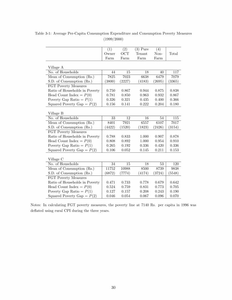
Table 3-1: Average Per-Capita Consumption Expenditure and Consumption Poverty Measures(1999/2000)

(1) (2) (3) Pure (4)Owner OCT Tenant Non- TotalFarm Farm Farm Farm

Village ANo. of Households 44 15 18 40 117Mean of Consumption (Rs.) 7825 7023 6638 6479 7079S.D. of Consumption (Rs.) (3800) (2227) (4183) (2695) (3365)FGT Poverty MeasuresRatio of Households in Poverty 0.750 0.867 0.944 0.875 0.838Head Count Index = P (0) 0.781 0.850 0.963 0.932 0.867Poverty Gap Ratio = P (1) 0.326 0.321 0.435 0.400 0.366Squared Poverty Gap = P (2) 0.156 0.141 0.222 0.204 0.180

Village BNo. of Households 33 12 16 54 115Mean of Consumption (Rs.) 8401 7921 6557 6107 7017S.D. of Consumption (Rs.) (4422) (1520) (1823) (2426) (3154)FGT Poverty MeasuresRatio of Households in Poverty 0.788 0.833 1.000 0.907 0.878Head Count Index = P (0) 0.808 0.892 1.000 0.954 0.910Poverty Gap Ratio = P (1) 0.265 0.192 0.336 0.420 0.336Squared Poverty Gap = P (2) 0.106 0.052 0.145 0.211 0.153

Village CNo. of Households 34 15 18 53 120Mean of Consumption (Rs.) 11752 10988 8500 8739 9838S.D. of Consumption (Rs.) (6872) (7774) (4174) (3724) (5548)FGT Poverty MeasuresRatio of Households in Poverty 0.471 0.733 0.778 0.679 0.642Head Count Index = P (0) 0.524 0.759 0.831 0.773 0.705Poverty Gap Ratio = P (1) 0.127 0.157 0.208 0.243 0.190Squared Poverty Gap = P (2) 0.046 0.054 0.067 0.096 0.070

Notes: In calculating FGT poverty measures, the poverty line at 7140 Rs. per capita in 1996 wasdeflated using rural CPI during the three years.

30

Table 3-2: Average Per-Capita Consumption Expenditure and Consumption Poverty Measures(1996)

No. of ConsumptionHouse- Level FGT Poverty Measuresholds Mean (S.D.) P (H)$ P (0) P (1) P (2)

All Sample Households 354 5858 (2889) 0.740 0.792 0.308 0.143By Village

Village A 119 5243 (2268) 0.807 0.885 0.369 0.174Village B 116 5550 (2656) 0.750 0.796 0.332 0.167Village C 119 6772 (3411) 0.664 0.677 0.214 0.083

By Household Type(1) Owner Farm 125 6338 (3534) 0.704 0.750 0.285 0.133(2) OCT Farm 50 6514 (2796) 0.600 0.721 0.281 0.123(3) Pure Tenant Farm 60 5718 (2448) 0.717 0.767 0.304 0.139(4) Non-Farm 119 5148 (2159) 0.849 0.892 0.352 0.167

Notes: In calculating FGT poverty measures, the poverty line at 7140 Rs. per capita in 1996 wasused. Estimated from 1996 household data described in Kurosaki and Hussain (1999).$ P (H) stands for “Ratio of Households in Poverty.”

31

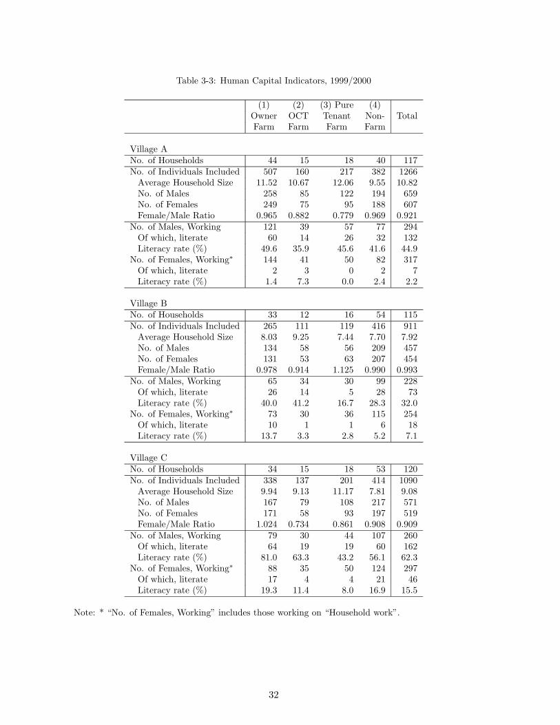
Table 3-3: Human Capital Indicators, 1999/2000

(1) (2) (3) Pure (4)Owner OCT Tenant Non- TotalFarm Farm Farm Farm

Village ANo. of Households 44 15 18 40 117No. of Individuals Included 507 160 217 382 1266

Average Household Size 11.52 10.67 12.06 9.55 10.82No. of Males 258 85 122 194 659No. of Females 249 75 95 188 607Female/Male Ratio 0.965 0.882 0.779 0.969 0.921

No. of Males, Working 121 39 57 77 294Of which, literate 60 14 26 32 132Literacy rate (%) 49.6 35.9 45.6 41.6 44.9

No. of Females, Working∗ 144 41 50 82 317Of which, literate 2 3 0 2 7Literacy rate (%) 1.4 7.3 0.0 2.4 2.2

Village BNo. of Households 33 12 16 54 115No. of Individuals Included 265 111 119 416 911




Village CNo. of Households 34 15 18 53 120No. of Individuals Included 338 137 201 414 1090




Note: * “No. of Females, Working” includes those working on “Household work”.

32

Table 3-4: School Enrollment of Children, 1999/2000

(1) (2) (3) (4) Total

Village ANo. of Households 44 15 18 40 117No. of Males, Age: 5-10 50 11 28 40 129

Of which, enrolled 30 4 10 14 58Enrollment ratio (%) 60.0 36.4 35.7 35.0 45.0

No. of Females, Age: 5-10 46 16 21 45 128Of which, enrolled 11 3 1 2 17Enrollment ratio (%) 23.9 18.8 4.8 4.4 13.3

Village BNo. of Households 33 12 16 54 115No. of Males, Age: 5-10 28 6 10 44 88



Village CNo. of Households 34 15 18 53 120No. of Males, Age: 5-10 27 17 21 26 91



33

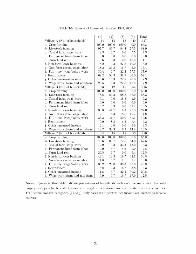
Table 3-5: Sources of Household Income, 1999/2000

(1) (2) (3) (4) TotalVillage A (No. of households) 44 15 18 40 117a. Crop farming 100.0 100.0 100.0 0.0 65.8b. Livestock farming 97.7 86.7 94.4 77.5 88.9c. Casual farm wage work 2.3 6.7 0.0 7.5 4.3d. Permanent hired farm labor 0.0 0.0 0.0 0.0 0.0e. Farm land rent 13.6 13.3 0.0 12.5 11.1f. Non-farm, own business 18.2 13.3 27.8 10.0 16.2g. Non-farm casual wage labor 18.2 33.3 16.7 5.0 15.4h. Full-time, wage/salary work 36.4 6.7 22.2 57.5 37.6i. Remittances 68.2 53.3 38.9 40.0 52.1j. Other unearned income 13.6 13.3 27.8 20.0 17.9k. Wage work, farm and non-farm 20.5 13.3 27.8 12.5 17.9Village B (No. of households) 33 12 16 54 115a. Crop farming 100.0 100.0 100.0 0.0 53.0b. Livestock farming 78.8 83.3 68.8 37.0 58.3c. Casual farm wage work 6.1 0.0 18.8 1.9 5.2d. Permanent hired farm labor 0.0 0.0 0.0 0.0 0.0e. Farm land rent 18.2 8.3 0.0 22.2 16.5f. Non-farm, own business 30.3 41.7 6.3 27.8 27.0g. Non-farm casual wage labor 12.1 8.3 18.8 16.7 14.8h. Full-time, wage/salary work 33.3 41.7 50.0 61.1 49.6i. Remittances 0.0 8.3 6.3 7.4 5.2j. Other unearned income 6.1 0.0 0.0 5.6 4.3k. Wage work, farm and non-farm 18.2 33.3 6.3 14.8 16.5Village C (No. of households) 34 15 18 53 120a. Crop farming 100.0 100.0 100.0 0.0 55.8b. Livestock farming 70.6 86.7 77.8 34.0 57.5c. Casual farm wage work 2.9 13.3 33.3 13.2 13.3d. Permanent hired farm labor 0.0 6.7 5.6 1.9 2.5e. Farm land rent 26.5 6.7 0.0 9.4 12.5f. Non-farm, own business 44.1 13.3 16.7 32.1 30.8g. Non-farm casual wage labor 11.8 6.7 11.1 9.4 10.0h. Full-time, wage/salary work 38.2 20.0 33.3 62.3 45.8i. Remittances 8.8 13.3 16.7 3.8 8.3j. Other unearned income 11.8 6.7 22.2 30.2 20.8k. Wage work, farm and non-farm 5.9 6.7 16.7 17.0 12.5

Notes: Figures in this table indicate percentages of households with each income source. For self-employment jobs (a, b, and f), cases with negative net income are also treated as income sources.For income transfer categories (i and j), only cases with positive net income are treated as incomesources.

34

Table 3-6: Composition of Household Income by Source, 1999/2000

(1) (2) (3) (4) TotalVillage A

Mean per-capita income in Rs. 7950 7947 7133 6611 7366(S.D.) (6385) (5601) (4356) (3822) (5193)

a. Crop farming 9.3 20.1 12.3 0.0 9.0b. Livestock farming 4.0 5.1 11.0 4.4 5.4c. Casual farm wage work 0.1 0.3 0.0 1.4 0.5d. Permanent hired farm labor 0.0 0.0 0.0 0.0 0.0e. Farm land rent 1.2 0.5 0.0 1.1 0.9f. Non-farm, own business 10.1 9.2 13.0 14.8 11.7g. Non-farm casual wage labor 2.6 8.2 8.2 1.3 4.0h. Full-time, wage/salary work 16.3 5.1 13.3 36.2 19.4i. Remittances 51.4 46.7 24.1 27.3 39.9j. Other unearned income 0.4 0.1 3.5 2.5 1.4k. Wage work, farm and non-farm 4.5 4.7 14.6 11.2 7.9Village B


a. Crop farming 27.5 20.4 28.0 0.0 15.6b. Livestock farming 8.3 15.0 11.3 5.8 9.0c. Casual farm wage work 1.2 0.0 7.1 0.7 1.3d. Permanent hired farm labor 0.0 0.0 0.0 0.0 0.0e. Farm land rent 7.7 1.0 0.0 3.7 4.1f. Non-farm, own business 28.2 34.2 6.3 31.4 28.7g. Non-farm casual wage labor 2.3 1.0 5.0 4.2 3.0h. Full-time, wage/salary work 17.1 14.3 37.7 38.7 26.6i. Remittances -0.5 4.8 3.2 5.0 3.0j. Other unearned income -1.1 -1.0 -0.5 0.3 -0.5k. Wage work, farm and non-farm 9.2 10.3 1.9 10.3 9.2Village C


a. Crop farming 21.0 37.4 25.1 0.0 17.5b. Livestock farming 5.3 8.8 6.4 3.2 5.3c. Casual farm wage work 0.3 1.0 5.7 5.7 2.8d. Permanent hired farm labor 0.0 1.4 1.9 0.5 0.6e. Farm land rent 8.9 1.7 0.0 2.7 4.6f. Non-farm, own business 33.5 21.1 15.4 22.7 25.7g. Non-farm casual wage labor 2.5 1.8 2.2 2.4 2.3h. Full-time, wage/salary work 25.0 5.6 23.4 50.6 29.8i. Remittances 2.4 19.9 13.2 0.4 6.1j. Other unearned income 0.4 0.2 1.0 5.8 2.2k. Wage work, farm and non-farm 0.7 1.0 5.5 6.0 3.0

Notes: Figures in this table indicate percentage composition of each income source in the totalhousehold income. Categories a, b, f, i, and j could take negative values. Categories i and j indicatenet values.

35

Table 3-7: Indicators of Household-Level Job Diversification, 1999/2000

(1) (2) (3) (4) Total

Village ANumber of jobs per household 3.20 2.87 2.83 1.60 2.56Percentage of households

engaged in non-farm activities 88.6 93.3 77.8 97.5 90.6

Village BNumber of jobs per household 2.06 2.50 2.19 1.63 1.92Percentage of households


Village CNumber of jobs per household 2.47 1.93 2.56 1.87 2.15Percentage of households


Note: In calculating the “Number of jobs per household,” a self-employed activity (a, b, and f inTables 3-5 and 3-6) is counted as one job regardless of the number of family members involved inthat business; in the case of full-time wage/salary work and remittance senders (h and i), the numberof such workers is added directly. Among agriculture-related activities, casual farm labor (c) andpermanent hired labor (d) are distinguished because their mode of payment is different.

36

Table 3-8A: Adjustment to Economic Risk, Village A, 1999/2000

(1) (2) (3) (4) TotalNo. of Households 44 15 18 40 117Economically best year [1996/97 - 1998/99]

1996/97 3 6 5 8 221997/98 30 6 10 10 561998/99 3 2 1 0 6No best year 8 1 2 21 32

Reason for the best year1. Good crop harvest 34 13 15 4 662. Good prices of farm produce 3 1 0 3 73. More wage income due to wage increases 3 2 0 5 104. More family members obtained jobs 1 1 1 7 105. Increase in remittances 5 2 2 5 146. Inheritance 1 0 0 0 1Adjustment in the best year1. More consumption of food 17 6 9 11 432. More consumption of non-food 1 6 2 0 4 123. Less work outside, more leisure time 1 1 0 3 54. Saved in financial institutions 2 0 0 0 0 05. Purchased gold and jewelry 0 0 1 1 26. Purchased livestock 2 0 2 1 57. Purchased land 0 1 0 0 18. More food storage 27 11 11 4 539. Helped others 3 4 0 2 1 710. More education for children 1 1 1 1 4Economically worst year [1996/97 - 1998/99]

1996/97 7 3 1 3 141997/98 3 6 2 8 191998/99 30 4 11 14 59No worst year 8 1 4 17 30

Reason for the worst year1. Bad crop harvest 35 13 12 6 662. Bad prices of farm produce 2 0 1 1 43. Less wage income due to wage decreases 2 2 0 7 114. Less family members with jobs 4 2 2 8 165. Decrease in remittances 2 0 1 3 66. Inheritance 0 0 0 0 0Adjustment in the worst year1. Less consumption of food 18 7 7 15 472. Less consumption of non-food 1 4 1 1 4 103. More work outside, less leisure time 2 0 0 1 34. Dis-saved in financial institutions 4 0 0 0 0 05. Sold gold and jewelry 0 0 0 0 06. Sold livestock 1 0 2 1 47. Sold land 0 0 0 1 18. Less food storage 29 10 8 4 519. Helped by others 3 10 1 8 10 2910. Less education for children 0 0 1 0 1

37

Table 3-8B: Adjustment to Economic Risk, Village B, 1999/2000


1996/97 4 0 1 2 71997/98 3 4 5 4 161998/99 6 3 4 4 17No best year 21 5 6 44 76


1996/97 2 0 1 2 51997/98 6 2 3 5 161998/99 14 5 9 22 50No worst year 14 5 3 26 48


38

Table 3-8C: Adjustment to Economic Risk, Village C, 1999/2000


1996/97 4 2 1 3 101997/98 6 3 5 9 231998/99 11 7 5 8 31No best year 13 4 7 31 55


1996/97 2 0 2 3 71997/98 5 2 0 5 121998/99 12 5 9 21 47No worst year 11 9 7 17 44


39

Notes to Table 3-8:Figures in this table show the number of households indicating the choices (multiple choices for “Rea-sons” and “Adjustments”).(1) The category of “non-food” consumption includes durable goods such as house building.(2) “Saved in financial institutions” includes cases where households paid back debts from financialinstitutions.(3) “Helped (by) others” includes reciprocity arrangements such as giving informal credit and trans-fers, paying back informal debts, or obtaining informal credit and transfers.(4) “Dis-saved in financial institutions” includes cases where households obtained credit from financialinstitutions.

40

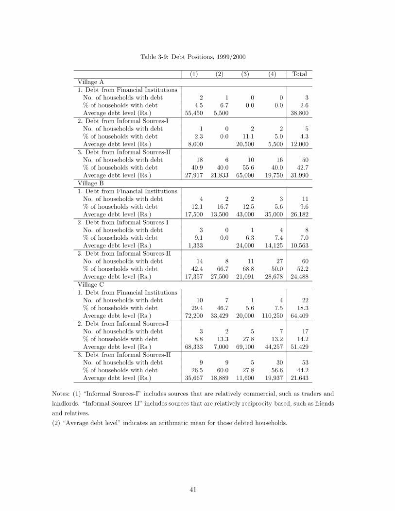
Table 3-9: Debt Positions, 1999/2000

(1) (2) (3) (4) TotalVillage A1. Debt from Financial Institutions

No. of households with debt 2 1 0 0 3% of households with debt 4.5 6.7 0.0 0.0 2.6Average debt level (Rs.) 55,450 5,500 38,800

2. Debt from Informal Sources-INo. of households with debt 1 0 2 2 5% of households with debt 2.3 0.0 11.1 5.0 4.3Average debt level (Rs.) 8,000 20,500 5,500 12,000

3. Debt from Informal Sources-IINo. of households with debt 18 6 10 16 50% of households with debt 40.9 40.0 55.6 40.0 42.7Average debt level (Rs.) 27,917 21,833 65,000 19,750 31,990

Village B1. Debt from Financial Institutions

No. of households with debt 4 2 2 3 11% of households with debt 12.1 16.7 12.5 5.6 9.6Average debt level (Rs.) 17,500 13,500 43,000 35,000 26,182

2. Debt from Informal Sources-INo. of households with debt 3 0 1 4 8% of households with debt 9.1 0.0 6.3 7.4 7.0Average debt level (Rs.) 1,333 24,000 14,125 10,563


Village C1. Debt from Financial Institutions

No. of households with debt 10 7 1 4 22% of households with debt 29.4 46.7 5.6 7.5 18.3Average debt level (Rs.) 72,200 33,429 20,000 110,250 64,409

2. Debt from Informal Sources-INo. of households with debt 3 2 5 7 17% of households with debt 8.8 13.3 27.8 13.2 14.2Average debt level (Rs.) 68,333 7,000 69,100 44,257 51,429


Notes: (1) “Informal Sources-I” includes sources that are relatively commercial, such as traders andlandlords. “Informal Sources-II” includes sources that are relatively reciprocity-based, such as friendsand relatives.(2) “Average debt level” indicates an arithmatic mean for those debted households.

41

Human Capital and Elimination of Rural Poverty: A Case ...kurosaki/ids1999r.pdf · From descriptive...

Documents

Transcript of Human Capital and Elimination of Rural Poverty: A Case ...kurosaki/ids1999r.pdf · From descriptive...