HST hot Jupiter transmission spectral survey: detection of ...showman/publications/... · HST hot...

MNRAS 435, 3481–3493 (2013) doi:10.1093/mnras/stt1536Advance Access publication 2013 September 16

HST hot Jupiter transmission spectral survey: detection of waterin HAT-P-1b from WFC3 near-IR spatial scan observations

H. R. Wakeford,1‹ D. K. Sing,1 D. Deming,2 N. P. Gibson,3 J. J. Fortney,4

A. S. Burrows,5 G. Ballester,6 N. Nikolov,1 S. Aigrain,7 G. Henry,8 H. Knutson,9

A. Lecavelier des Etangs,10 F. Pont,1 A. P. Showman,6 A. Vidal-Madjar10

and K. Zahnle11

1Astrophysics Group, School of Physics, University of Exeter, Stocker Road, Exeter EX4 4QL, UK2Department of Astronomy, University of Maryland, College Park, MD 20742, USA3ESO Karl-Schwarzschild-Strasse 2, D-85748 Garching bei Munchen, Germany4Department of Astronomy and Astrophysics, University of California, Santa Cruz, CA 95064, USA5Department of Astrophysical Sciences, Princeton University, Princeton, NJ 08544-1001, USA6Lunar and Planetary Lab, University of Arizona, Tucson, AZ 85721, USA7Department of Physics, University of Oxford, Denys Wilkinson Building, Keble Road, Oxford OX1 3RH, UK8Tennessee State University, Nashville, TN 37203-3401, USA9Division of Geological and Planetary Sciences, California Institute of Technology, Pasadena, CA 91125, USA10Institut d’Astrophysique de Paris, CNRS, 98 bis Boulevard Arago, F-75014 Paris, France11NASA Ames Research Center, Moffett Field, CA 94035, USA

Accepted 2013 August 14. Received 2013 August 9; in original form 2013 April 4

ABSTRACTWe present Hubble Space Telescope near-infrared transmission spectroscopy of the transitinghot-Jupiter HAT-P-1b. We observed one transit with Wide Field Camera 3 using the G141 low-resolution grism to cover the wavelength range 1.087–1.678 µm. These time series observationswere taken with the newly available spatial-scan mode that increases the duty cycle by nearly afactor of 2, thus improving the resulting photometric precision of the data. We measure a planet-to-star radius ratio of Rp/R∗ = 0.117 09 ± 0.000 38 in the white light curve with the centreof transit occurring at 245 6114.345 ± 0.000 133 (JD). We achieve S/N levels per exposureof 1840 (0.061 per cent) at a resolution of �λ = 19.2 nm (R ∼ 70) in the 1.1173–1.6549 µmspectral region, providing the precision necessary to probe the transmission spectrum ofthe planet at close to the resolution limit of the instrument. We compute the transmissionspectrum using both single target and differential photometry with similar results. The resultanttransmission spectrum shows a significant absorption above the 5σ level matching the 1.4 µmwater absorption band. In solar composition models, the water absorption is sensitive tothe ∼1 m bar pressure levels at the terminator. The detected absorption agrees with thatpredicted by a 1000 K isothermal model, as well as with that predicted by a planetary-averagedtemperature model.

Key words: techniques: spectroscopic – planets and satellites: atmospheres – planetarysystems.

1 IN T RO D U C T I O N

The understanding of exoplanetary atmospheres has advanced con-siderably in the last decade, thanks in part to the spectroscopic ob-servations of transiting exoplanets. During a transit, when a planetpasses between Earth and its host star, a small fraction of the starlightis blocked by the planet; this can then be seen as a characteristic

� E-mail: [email protected]

dip in the transit light curve. Transiting planets offer a unique op-portunity to study their atmospheres through a method called trans-mission spectroscopy. As the starlight passes through their upperatmospheres characteristic spectral signatures are superimposed onthe light as it is absorbed or scattered. The absorption and opti-cal depth of the atmosphere is dependent on wavelength, as is thealtitude at which the planet is opaque to starlight. Features ob-served in the transmission spectrum place strong constraints on thepossible species in the atmosphere (e.g. Seager & Sasselov 2000;Charbonneau et al. 2002).

C© 2013 The AuthorsPublished by Oxford University Press on behalf of the Royal Astronomical Society

at University of A

rizona on October 31, 2013

http://mnras.oxfordjournals.org/

Dow

nloaded from

at University of A



Dow

nloaded from

at University of A



Dow

nloaded from

at University of A



Dow

nloaded from

at University of A



Dow

nloaded from

at University of A



Dow

nloaded from

at University of A



Dow

nloaded from

at University of A



Dow

nloaded from

at University of A



Dow

nloaded from

at University of A



Dow

nloaded from

at University of A



Dow

nloaded from

at University of A



Dow

nloaded from

at University of A



Dow

nloaded from














3482 H. R. Wakeford et al.

A range of atomic and molecular species have been identifiedin exoplanetary atmospheres through transmission spectroscopy,with a majority having been identified in the upper and lower at-mospheres of HD 189733b and HD 209458b, which remain themost studied exoplanets to date. Ground- and space-based obser-vations ranging from the ultraviolet (UV) to the infrared (IR) havebeen able to probe both the lower and extended upper atmosphereof these two exoplanets (for example: Vidal-Madjar et al. 2003,2004; Narita et al. 2005; Pont et al. 2007; Tinetti et al. 2007; Grill-mair et al. 2008; Redfield et al. 2008; Snellen et al. 2008; Swain,Vasisht & Tinetti 2008; Desert et al. 2009; Linsky et al. 2010; Singet al. 2011; Gibson et al. 2012; Lecavelier des Etangs et al. 2012;Ben-Jaffel & Ballester 2013; Deming et al. 2013; Waldmann et al.2013).

H2O is a key molecule for constraining hot-Jupiter atmospheres.It is predicted that the C/O ratio plays a pivotal role in the relativeabundances of H2O and the other spectroscopically important CH4,CO, CO2, C2H4 and HCN molecules in the atmospheres of close-ingiant planets (e.g. Seager & Sasselov 2000; Madhusudhan 2012).Moses et al. (2013) have analysed transit and eclipse observationsof a number of transiting hot Jupiters, finding that some extrasolargiant planets could have unexpectedly low abundance of H2O dueto high C/O ratios. Atmospheres with solar elemental abundancesin thermochemical equilibrium are expected to have abundant watervapour, and disequilibrium processes like photochemistry are notable to deplete water sufficiently in the IR photosphere of these plan-ets to explain the observations (see Moses et al. 2013 and referencesthere in). Extinction from clouds and hazes could also significantlymask absorption signatures of water, however, this would also maskother molecular species making emission spectra appear more likea blackbody (Fortney 2005; Pont et al. 2013).

In this paper, we present the transmission spectrum of HAT-P-1b based on one transit observation between 1.1 and 1.7 µm usingHubble Space Telescope (HST) Wide Field Camera 3 (WFC3) inspatial-scan mode. HST/WFC3 IR observations at 1.1–1.7 µm probeprimarily the H2O absorption band at 1.4 µm. These observationsare among the first results from a large survey with HST probingthe transmission spectra, from the optical to near-IR (NIR), of eighthot-Jupiter exoplanets (GO programme 12473, P.I. D. Sing). HAT-P-1b is a low-density hot Jupiter orbiting a single member of avisual stellar binary (Bakos et al. 2007). HAT-P-1b orbits its hoststar with a period of 4.5 d at a distance of 0.055 au. It has a radiussimilar to that of HD 209458b with a somewhat lower mean densitywith a mass of 0.54 MJ. Spitzer Infrared Array Camera (IRAC)secondary eclipse measurements show that the atmosphere is bestfit with a modest temperature inversion with a maximum daysidetemperature of 1550 K, assuming zero albedo, a uniform temper-ature over the dayside hemisphere, and no transport to the night-side (Todorov et al. 2010). Ks-band secondary-eclipse observationshave also been conducted by the GROUnd-based Secondary Eclipseproject with an estimated brightness temperature of 2136 ± 150 Kand for an eclipse depth of 0.109 ± 0.025 per cent although there arestill visible systematics that remain in the fit (de Mooij et al. 2011).

In Section 2, we outline the observations and the use of spatial-scan mode; in Section 3, we present the analysis of the extractedlight curves; in Section 4, we compare the result with atmosphericmodels and in Section 5, we state our conclusions.

2 O BSERVATIONS

Observations of HAT-P-1 were conducted in the NIR withHST/WFC3. WFC3’s IR channel consists of a 1024 × 1024 pixel

Figure 1. Cut-out of WFC3 G141 grism exposure with the spatial-scanspectra of the HAT-P-1 extraction window outlined in blue (top) and theG0 stellar companion outlined in green (bottom). To the left of HAT-P-1’sspectra is the background subtraction region (outlined in a yellow box).

Teledyne HgCdTe detector that can be paired with any of 15 filtersor two low-resolution grisms (Dressel et al. 2010). Each exposureis compiled from multiple non-destructive reads (NSAMP) at eitherthe full array or a sub-array. Although the standard WFC3 config-uration is not particularly efficient for high S/N time series data,as buffer dumps are long and the point spread function covers veryfew pixels (low S/N per exposure), the instrumental systematics arenoticeably lower than for Near Infrared Camera and Multi-ObjectSpectrometer (NICMOS) as WFC3 does not suffer from strong in-trapixel sensitivities. WFC3 also has a factor of 2 improvement onsensitivity over NICMOS with a much higher throughput and lowerread noise (e.g. WFC3 Instrument Handbook).

The observations started on 2012 July 5th at 15:17 using the IRG141 grism in spatial-scan mode over five HST orbits. We gatheredexposures using 512 × 512 pixel sub-arrays with an NSAMP = 4readout sequence and exposure times of 46.69 s.

HAT-P-1 is the dimmer member of a double G0/G0 star sys-tem, ADS 16402, separated by 11.2 arcsec (Bakos et al. 2011).Both stars are clearly resolved in the 68 arcsec × 68 arcsec field ofview of HST/WFC3’s spatial-scan spectra and are easily extractedseparately in the analysis (see Figs 1 and 2). This provides the op-portunity to perform differential photometry on HAT-P-1 using thecompanion’s signal which can reduce observational systematics inthe data (see Figs 3 and 4).

Figure 2. Top: spectra extracted from HST/WFC3 ‘ima images for HAT-P-1 (blue lower) and its G0 binary companion (green upper). Bottom: theresultant spectrum from differential photometric analysis; the vertical dashedlines define the wavelength range used in the spectroscopic analysis.

Detection of water in HAT-P-1b 3483

Figure 3. The raw white light curve for the reference and target star as wellas the raw differential light curve produced by dividing the target star lightcurve by the reference star light curve. Overplotted in red are the Mandeland Agol (2002) limb-darkened transit models. The different light curveshave been artificially shifted for clarity.

Figure 4. Upper: breathing-corrected light curves for both single targetphotometry (top curve) and differential photometry (bottom curve). Thesub-plot shows the red noise for both single target (blue) and differentialphotometry (black) showing that time correlated noise is decreased whendifferential photometry is performed. Lower: corresponding residuals forboth fits showing the decrease in errors and deviation from the mean whenapplying differential photometry to the data.

2.1 Spatial scanning

We present some of the first results from WFC3 using the spatial-scan mode to observe exoplanetary transits. The WFC3 spatialscanning involves nodding the telescope during an exposure tospread the light along the cross-dispersion axis, resulting in a highernumber of photons by a factor of 10 per exposure while consider-ably reducing overheads. This also increases the time of satura-tion of the brightest pixels, and allows for longer exposure times(McCullough 2011). Our observations were conducted with a scanrate of 1.07 pixels per second, where 1 pixel = 0.13 arcsec and thusspanning ∼50 pixels over each 46.69 s exposure. The duty cycleof the observations improved from 26 per cent in non-spatial-scanmode to 40 per cent.

The raw light curves of some WFC3 non-spatial-scan observa-tions (e.g. Berta et al. 2012) have been dominated by a systematicincrease in intensity during each group of exposures obtained be-tween buffer dumps referred to as the ‘hook’ effect. It has beenfound that the ‘hook’ is, on average, zero when the count rate is

less than about 30 000 electrons per pixel (Deming et al. 2013). Weobserve a maximum raw count rate of 25 000 electrons per pixelin our target star and a rate of ∼30 000 electrons per pixel for thecompanion star with no evidence for a significant ‘hook’ effect inthe reduced data of either star (see Fig. 4).

3 A NA LY SIS

We used the ‘ima’ outputs from WFC3’s Calwf3 pipeline. For eachexposure, Calwf3 conducts the following processes: bad pixel flag-ging, reference pixel subtraction, zero-read subtraction, dark currentsubtraction, non-linearity correction, flat-field correction, as well asgain and photometric calibration. The resultant images are in unitsof electrons per second.

Subsequent data analysis is conducted with the first orbit removed(26 exposures), as it suffers from thermal breathing systematic ef-fects that require time to settle, all previous transit studies have useda similar strategy (Brown et al. 2001; Charbonneau et al. 2002; Singet al. 2011). This leaves 86 exposures over the remaining four or-bits with a total of 30 in transit exposures. The mid-time of eachexposure was converted into BJDTBD for use in the transit lightcurves.

We used a box around each spectral image shown in Fig. 1. Thespectra were extracted using custom IDL procedures, similar to IRAF’sAPALL procedure, using an aperture of ±23 pixels from the centralrow, determined by minimizing the standard deviation across theaperture.

This 47 pixel aperture is slightly shorter than the total heightof the spectrum to utilize pixels having similar exposure levelsto the maximum possible degree. The aperture is traced arounda computed centring profile, which was found to be consistent inthe y-axis within an error of 0.01 pixels. Background subtractionwas applied using the region to the left of the HAT-P-1 spectrum(shown in Fig. 1), because the region above and below each spectrumcontains significant count levels which added noise to the resultantspectrum.

3.1 Wavelength calibration

For wavelength calibration, direct images were taken in the F139Mnarrow band filter at the beginning of the observations for a referenceof the absolute position (Xref, Yref) of the target star. We assumed thatall pixels in the same column have the same effective wavelength,as the spatial scan varied in the Xref by less than one pixel, giving aspectral range of 1.087–1.678 µm.

This wavelength range was later restricted to 1.1173–1.6549 µmfor the spectroscopic light-curve fits as the strongly sloped edgescovered by the grism response exhibit greater wavelength jitterwhere the intensities increase towards the edge of the bandpass (seeFig. 2).

To calculate the wavelength corresponding to each pixel alongthe x-direction, we applied a linear fit to the wavelength solution.The wavelength solution is a function of the Xref and Yref positiongiven by

λ(x) = a0 + a1 × Xref

and

λ(pixel) = λ(x) + (Yref dispersion × XPixel), (1)

where, Xref is taken from the filter image, a0 and a1 are taken fromtable 5 in Kuntschner et al. (2009), and Yref dispersion is found in fig. 6


of Kuntschner et al. (2009) using the Yref position from the filterimage.

The G141 grism images contain both the zeroth-order and thefirst-order spectra for both stars. Each first-order spectrum spans128 pixels with a dispersion of 4.65 nm pixel−1 and the separationbetween the two stellar spectra was 23 pixels in the y-axis and33 pixels in the x-axis (see Fig. 1).

Using the zeroth-order spectrum, we characterized the shift in Yref

over the course of the observations to monitor any shift in wave-length of the spectral trace. We observed a ±0.2 pixel column shiftin the wavelength direction over the whole observing period. Thiscorresponded to 0.001 86 µm or an ∼10 per cent wavelength shiftfor each spectral bin over the span of the observations. We there-fore adjusted the wavelength solution to use the average wavelengthof the visit for each spectral bin. The observations, however, wererelatively insensitive to sub-pixel wavelength shifts while the waterspectral band spans a much larger wavelength range.

Larger wavelength shifts were observed by Deming et al. (2013)over the course of their observations of planetary transits whichalso revealed evidence of undersampling of the grism resolutionby the pixel grid changing gradually and smoothly as a functionof wavelength shift. To determine if our data contained similarundersampling, we compared a number of the spectral lines from thestart and end of the observations (separated by over 3 h) at a numberof positions along the scanned spectra. Unlike the results found byDeming et al. (2013), we see no flattening of the strong Paschen-beta stellar line at 1.28 µm due to an undersampling effect. To helpreduce the effects of any unidentified undersampling, we moderatelybinned our spectra effectively smoothing out any undersamplinginherent in our data.

3.2 Limb darkening

To accurately model the transit light curves, stellar limb darkeninghas to be carefully considered. The light curves were fit using theMandel & Agol (2002) limb-darkened analytic transit model. Wecalculated limb-darkening coefficients from a 3D time-dependenthydrodynamical model (Hayek et al. 2012) over the wavelengthrange 1.1–1.7 µm with the coefficients calculated separately foreach spectral band. We also computed the limb-darkening coef-ficients using Kurucz stellar models for a star at Teff = 6000 K,log g = 4.5 and [Fe/H] = +0.1 (Torres, Winn & Holman 2008).The coefficients were calculated following Sing (2010) using anon-linear limb-darkening law given by

I (μ)

I (1)= 1 −

4∑n=1

cn(1 − μn2 ), (2)

where I(1) is the intensity at the centre of the stellar disc andμ = cos(θ ) is the angle between the line of sight and the emer-gent intensity.

The 3D model shows overall weaker limb darkening comparedto the 1D model (Hayek et al. 2012). The 3D model takes intoaccount convective motions in the stellar atmosphere resulting ina shallower vertical temperature profile. As the strength of limbdarkening is closely related to the vertical atmospheric temperaturegradient near the optical surface, the limb darkening slightly weak-ens for the shallower temperature profile. We find that this leads toan overall common shift in the derived planet-to-star radius ratio,with the shape of the transmission spectrum unaffected. We adoptthe 3D model as it provides an overall better fit between our Space

Telescope Imaging Spectrograph (STIS) and WFC3 data (Nikolovet al. 2013).

3.3 White light-curve fits

Prior to evaluating the transmission spectrum (from transit lightcurves in small spectral bins), we analysed the light curves summedover the entire wavelength range. The white light curve was usedto improve the general system parameters and quantitatively inves-tigate any instrumental systematics.

Systematics in the data that effect both the target and referencestar are partially removed by performing differential photometry,dividing target-star flux by the reference-star flux (see Fig. 3 fora comparison of the raw white light curves) reducing the residualscatter by a factor of 3. Furthermore, systematics present in the data,shown in the differential light curve of Fig. 3, display clear orbit-to-orbit trends of increasing flux within each HST orbit in the rawlight curve, which we attribute to a ‘breathing effect’, caused by thethermal expansion and contraction of HST during its orbit. We fitfor this similarly to Brown et al. (2001) and Sing et al. (2011), usinga seventh-order polynomial fit versus HST orbital phase. To avoidoverfitting the model as a result of adding parameters, we calculatedthe Bayesian Information Criterion (BIC) that adds a penalty termfor the number of parameters in the model, such that the significanceof each new parameter can be estimated. To account for breathingsystematics in the light curve, while avoiding overfitting, correc-tions were applied for a general slope over the entire light curve (acorrection over the HST visit) as well as a seventh-order polynomialin HST phase (a correction per HST orbit). No further trends, suchas the spectral trace position and timing of the central HST orbitalphase, were found to significantly improve the white light-curvefits, we therefore adopt these methods for our final white light fits(Fig. 4). We note a significant reduction, up to 65 per cent, in theparameters computed for the HST ‘breathing effect’ between singletarget and differential photometry showing that the ability to per-form differential photometry is an important aspect of this analysis.We find a decrease in the white light-curve residuals from a standarddeviation of 400 ppm to 160 ppm, placing a meaningful number onthe reference star as a calibrator. Telescope systematic errors affectthe science and calibrator stars in the same way to a precision ofone part per 2400; we address the residual systematics, 3.2 timeslarger than the photon noise in the case of these observations, usingindividual parameter analysis.

Throughout our analysis, we implemented a Levenberg–Marquardt least-squares minimization algorithm (L-M) to deter-mine the best-fitting parameters for both the planetary system andany systematics inherent in the data. This is done by using theMPFIT IDL routine by Markwardt (2009).

To corroborate these results, we also applied a Markov-chainMonte Carlo (MCMC) data analysis (Eastman, Gaudi & Agol2013). While the L-M computes the best-fitting χ2 value of theparameters by estimating the parameter errors from the covariancematrix calculated using numerical derivatives, the MCMC computesthe maximum likelihood of the parameter fit given a prior value andevaluates the posterior probability distribution for each parameterof the model. The MCMC routine uses a simplified quadratic limb-darkening model described by parameters allowed to vary withinthe Kurucz grid of stellar spectra as a function of emergent angle.EXOFAST (a fast exoplanetary fitting suite in IDL) also uses the stel-lar mass–radius relation of Torres et al. (2008) to constrain the stellarparameters, compared to fixed non-linear limb-darkening parame-ters used in the L-M with unconstrained stellar parameters. MCMC


Table 1. Table of constrained system parameters and errors (from Nikolovet al. 2013).

Parameter Value Uncertainties

Inclination (◦) 85.677 0.061Period (d) 4.465 299 74 0.000 000 55

a/R∗ 9.910 0.079Center of transit time (JD) 245 6114.345 307 0.000 18

can be more robust against finding local minima when searchingthe parameter space, where the L-M may get trapped.

Each method produces similar results within the errors with themain small differences arising primarily from the different limb-darkening fitting procedures.

The system parameters and uncertainties for, orbital inclination,orbital period, a/R∗ and centre of transit time were constrained usinga combined MCMC fit with three HST/STIS transit observations,two using G430L and one using G750L, and our WFC3 transit data(see Table 1).

The initial starting values for planetary and system parameterswere taken from Butler et al. (2006), Johnson et al. (2008) andTorres et al. (2008). The best-fitting light curve for the WFC3 transitalong with the uncertainties associated with the computation weredetermined using MPFIT giving a final white-light radius ratio ofRP/R∗ = 0.117 09 ± 0.000 38 (see Fig. 4).

We also fit the white light curve for single target photometry aswell as differential photometry as shown in Fig. 4. Without differ-ential photometry there are systematics in the data that increase theerrors and the deviation from the mean as shown by the residual plotat the bottom of Fig. 4, which shows that the differential photometryreduces the scatter in the residuals by a factor of 3. For both lightcurves the red noise, defined as the noise correlated with time (σ r),is estimated at each time-averaged bin of the light curve containingN points following Pont, Zucker & Queloz (2006),

σN =√

σ 2w

N+ σ 2

r , (3)

where σw is the white uncorrelated noise and σ N is the photonnoise. For our best-fitting light curve, we find σw = 1.49 × 10−4,with σ r = 4.97 × 10−5 using a bin size of N = 10 (see Fig. 4) witha photon noise level of 6.8 × 10−5.

Another method used to empirically correct for repeating sys-tematics between orbits is the divide-oot routine developed by Bertaet al. (2012). Divide-oot uses the out-of-transit orbits to compute aweighted average of the flux evaluated at each exposure within anorbit and divides the in-transit orbits by the template created. Thisrequires each of the in-transit exposures to be equally spaced intime with the out-of-transit exposures being used to correct them,so that each corresponding image has the same HST phase so thatadditional systematic effects are not introduced. Due to this con-straint, we were unable to perform the out-of-transit method as boththe in-transit and out-of-transit orbits contain a different number ofexposures with varied spacing between exposures.

The divide-oot method relies on the cancellation of common-mode systematic errors by operating only on the data themselvesusing simple linear procedures, relying on trends to be similar inthe time domain. A somewhat similar technique was adopted byDeming et al. (2013) for their analysis of WFC3 data relying oncommon trends in the wavelength domain. In Section 3.4.1, weadopt a similar method of subtracting white-light residuals from

each spectroscopic bin to corroborate our results from individualparameter analysis.

3.4 Spectroscopic light-curve fits

In order to understand and monitor the significance of each po-tentially common-mode systematic inherent in the WFC3 data, wedetermine a fit for each separate parameter as well as applyinga general common-mode analysis using the white-light residuals.We construct multiwavelength spectroscopic light curves by bin-ning the extracted spectra into 28 channels that are ∼4 pixels wide(�λ = 0.0192 µm) from 1.1173 to 1.6549 µm, which is close to theresolution of the G141 grism. To measure the transmission spectrumof HAT-P-1b, we conducted individual parameter fitting to each ofthe 28 light curves with a model in which Rp/R∗, a baseline flux anda seventh-order polynomial as a function of HST orbital phase areallowed to vary, and with the orbital inclination, orbital period, a/R∗and the centre of transit time fixed from the white light-curve fitting.To avoid overfitting the data, and to determine the consistency ofthe systematic model used, we computed the BIC number for eachspectroscopic bin. The systematic model with the lowest BIC wasfound to be consistent with that for the white light curve with littlesignificant variation in the computed BIC number between each ofthe spectroscopic bins. For limb-darkening coefficients, we againused the 3D models, fixed for each spectroscopic bin as listed inTable 2.

Similar to the white light curve, the seventh-order HST phasecorrection is used to account for breathing systematics. The fitted

Table 2. Transmission spectrum and limb-darkening coefficients for HAT-P-1b from WFC3/G141 using differential photometry and with common-mode removal of systematic errors (see Fig. 5).

λ Rp/R∗ c1 c2 c3 c4

(µm)

1.1269 0.116 56 ± 0.000 65 0.7301 −0.4003 0.3529 −0.12001.1461 0.116 32 ± 0.000 68 0.7271 −0.3993 0.3497 −0.11861.1653 0.116 43 ± 0.000 73 0.7253 −0.4005 0.3399 −0.11331.1845 0.114 93 ± 0.000 72 0.7192 −0.3703 0.3011 −0.09811.2037 0.116 40 ± 0.000 62 0.7157 −0.3677 0.2922 −0.09391.2229 0.117 15 ± 0.000 62 0.7273 −0.3759 0.2904 −0.09171.2421 0.116 56 ± 0.000 61 0.7315 −0.3769 0.2802 −0.08591.2613 0.115 28 ± 0.000 61 0.7349 −0.3673 0.2553 −0.07431.2805 0.116 39 ± 0.000 64 0.7639 −0.4002 0.2308 −0.05621.2997 0.115 19 ± 0.000 55 0.7470 −0.3724 0.2322 −0.06061.3189 0.116 51 ± 0.000 65 0.7482 −0.3768 0.2326 −0.05991.3381 0.117 44 ± 0.000 62 0.7560 −0.3824 0.2219 −0.05251.3573 0.116 56 ± 0.000 54 0.7710 −0.4064 0.2325 −0.05381.3765 0.117 26 ± 0.000 60 0.7885 −0.4378 0.2473 −0.05531.3957 0.117 16 ± 0.000 69 0.8061 −0.4666 0.2591 −0.05581.4149 0.118 07 ± 0.000 68 0.8292 −0.5034 0.2796 −0.05981.4341 0.117 80 ± 0.000 72 0.8522 −0.5623 0.3265 −0.07351.4533 0.117 19 ± 0.000 68 0.8706 −0.5906 0.3363 −0.07291.4725 0.118 23 ± 0.000 64 0.8915 −0.6199 0.3506 −0.07471.4917 0.117 31 ± 0.000 70 0.9156 −0.6854 0.4058 −0.09171.5109 0.117 98 ± 0.000 76 0.9470 −0.7560 0.4641 −0.10951.5301 0.117 37 ± 0.000 76 0.9788 −0.8295 0.5260 −0.12881.5493 0.116 50 ± 0.000 72 0.9714 −0.8486 0.5619 −0.14511.5685 0.116 05 ± 0.000 88 0.9875 −0.9154 0.6342 −0.17191.5877 0.114 66 ± 0.000 86 1.0501 −1.0948 0.8137 −0.23571.6069 0.116 16 ± 0.000 72 1.1217 −1.2570 0.9557 −0.28201.6261 0.114 74 ± 0.000 81 1.1263 −1.2696 0.9679 −0.28611.6453 0.115 71 ± 0.000 90 1.0649 −1.1631 0.8794 −0.2593


Figure 5. Top: the derived transmission spectrum of HAT-P-1b using differential photometry with individual parameter fitting. Bottom: spectroscopic lightcurve for each wavelength bin plotted vertically below the corresponding spectral depth measurement. The colours are used to guide the eye such that eachRp/R∗ measurement can be more easily matched with the corresponding light curve.

Rp/R∗ for each spectroscopic bin are listed in Table 2 along withthe corresponding limb-darkening parameters. Fig. 5 shows theresultant transmission spectrum as well as the light curves for dif-ferential photometry with individual parameter fitting. The binnedroot mean squared of the residuals for each wavelength-bin canbe seen in Fig. 6 shown relative to the photon noise of a repre-sentative spectral channel. We derived the transmission spectrumof HAT-P-1b for a wide range of wavelength bin sizes to test thefits and determine the achievable level of precision for the finaltransmission spectrum (see Fig. 7). Using differential photometrywith individual parameter fitting, we achieved S/N levels of ∼1840per image at a resolution of �λ = 19.2 nm (R ∼ 70). The result-ing transmission spectrum consists of 28 bins, each measured toa precision of about one planetary scaleheight. This demonstratesWFC3’s ability to measure the transmission spectrum of exoplanetsdown to the resolution of the instrument meaning that fine structurein the NIR spectrum of an exoplanetary atmosphere can potentiallybe measured.

3.4.1 Common-mode systematics

WFC3 exhibits common-mode systematic errors across the detectorthat are predominately not wavelength dependent. Common-mode

systematic trends usually do not highly impact the shape of the trans-mission spectrum, as each spectroscopic light-curve bin is similarlyaffected, and the relative planetary radius information is preserved.The common-mode trends can be seen in Fig. 8, which shows thatmost of the wavelength bins have a common HST coefficient within1σ of the computed white-light coefficients up to the seventh order.Fig. 9 shows this breathing correction for the white light curve over-plotted on the raw data showing the correction of a repeating trendin the data. In addition to the breathing systematic, there is also anon-repeating trend evident in the white-light residuals (see Figs 3and 4), specifically in the third and fourth orbits, that is present ineach wavelength band.

We therefore calculated the transmission spectrum using four dif-ferent methods, testing the effects of individual parameter fitting andthe cancelation of common-mode systematics using simple linearprocedures, for both differential and single-target photometry. Thefour different methods displayed in Fig. 10 show a common struc-ture to the transmission spectrum, indicating the significance of thespectral feature despite the assorted analysis techniques regardingdifferential analysis and common-mode removal of the systematictrends. We choose to quote final values for the transmission spec-tra from the analysis using differential photometry with individualparameter fitting, as it produces the highest quality light curve. The


Figure 6. Binned root mean square of the residuals for each spectroscopic bin (red, blue and green) plotted against the photon noise for the central wavelengthchannel of each plot (black). The residuals are calculated using differential photometry with individual parameter analysis.

Figure 7. Transmission spectrum of HAT-P-1b, derived using differentialphotometry with individual-parameter fitting, for �λ = 19.2 nm resolutionshown as black squares. Overplotted are the transmission spectra for arange of different wavelength resolution bins: �λ = 37.2 nm in green;�λ = 60.4 nm in pink and �λ = 74.4 nm in blue.

mean scatter of the residuals for all of the spectral bins is reducedby 10 per cent from single to differential photometry. In addition, areduction of ∼20 per cent is seen between common-mode removaland individual parameter analysis. There is also a significant re-duction in the red noise from σ r = 1.4 × 10−4 for differentialphotometry with common-mode removal down to σ r = 0.1 × 10−4

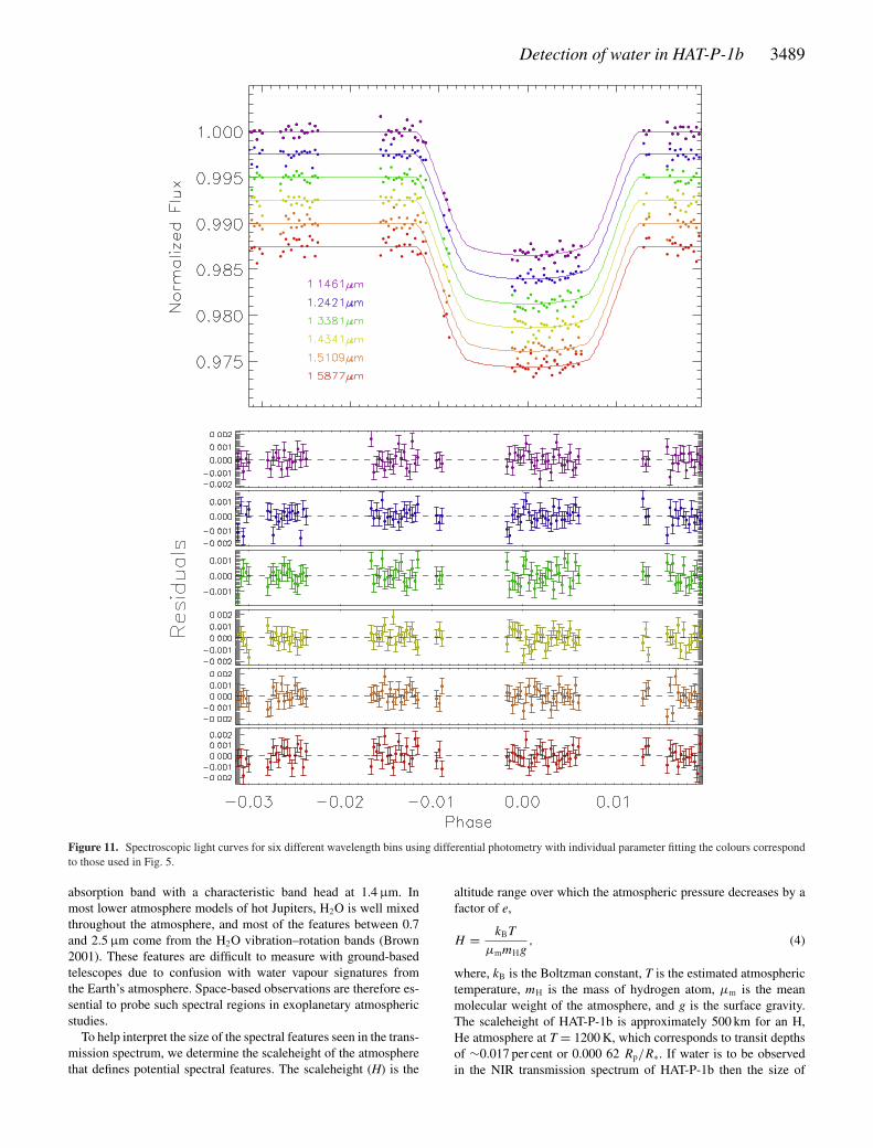
for differential photometry with individual parameter analysis (seeTable 3). In addition, by conducting both differential photometryand individual parameter analysis, we are thus able to better budgetfor the effects of the dominant thermal-breathing systematic on thetransit depths (through the use of the covariance matrix) and to betterunderstand the specific wavelength-dependent systematics inherentin the WFC3 data. While small, these can still potentially affectthe resultant spectrum obtained. We have therefore adopted themethod corresponding to Fig. 10(a) for further analysis and modelfitting. We also perform analysis on the transmission spectrum inFig. 10(b) discussed in Section 4.1.1 to corroborate the absorptionsignificance of the water absorption feature. Fig. 11 shows six ofthe 28 wavelength channels and their corresponding light curves fit-ted with differential photometry and individual parameter analysis;the residuals demonstrate that this method efficiently corrects forthe apparent common-mode trend seen in the white-light residualsin Fig. 4. We compute the transmission spectrum for differentialphotometry over a number of systematic models from fourth-orderpolynomial in HST orbital phase to a seventh-order polynomial inHST orbital phase adopted for this analysis (see Fig. 12). Fig. 12shows that systematic models fitting for HST orbital phase with apolynomial in the order between fourth and seventh do not changethe overall transmission spectrum while the BIC analysis favoursa seventh-order polynomial fit to the data. As we cannot use thedivide-oot routine, there are still some unmodelled systematics in


Figure 8. HST phase coefficients for each of the spectroscopic bins usingdifferential photometry individual parameter fitting. Top: the first- (black),second-order coefficients (red, squares). Middle-Top: the third-order (blackcircles) and fourth-order (red-circles) coefficients showing a near zero vari-ation over each wavelength bin. Middle-bottom: the fifth-order (black-stars)and sixth-order coefficient (red-stars). Bottom: the seventh-order HST phasecoefficient for each bin. Note the y-axis scale for each plot with the corre-sponding white-light coefficient marked as a solid line.

Figure 9. Raw white light curve with the breathing correction functionoverplotted as open squares (red) to show the fit to the orbit-to-orbit trendsevident in the data corresponding to the seventh-order parameter.

the white light-curve data resulting in a precision 2.9 times the pho-ton limit. Though we note that the absolute white-light precisionper exposure is ∼2.3 times better than Berta et al. (2012). Withthe use of optimized scheduling future observations can potentiallytake advantage of divide-oot with spatial scanning to increase thewhite-light performance. Our spectroscopic measurements comeclose to the photon noise limit of the detector with a mean errorwithin 12 per cent of the photon limit and a precision of Rp/R

∗ lessthan 0.0009 per spectral channel similar to that shown by Deminget al. (2013) and Swain et al. (2013).

Finally, to further characterize systematic effects in the data thatmay not have been accounted for, we injected a transit of con-stant depth (Rp/R∗ = 0.1142) into the reference star’s light curveand computed the transmission spectrum over the same wavelength

Figure 10. (a) Transmission spectrum of HAT-P-1b for differential photom-etry individual parameter fitting. (b) Single target photometry individualparameter fitting. (c) Differential photometry with common-mode fitting.(d) Single target photometry with common-mode fitting. While each spectrashow a common spectral shape the method used for figure (a) has lower rednoise and residual scatter for each spectroscopic bin and is therefore adoptedtransmission spectrum for further analysis.

Table 3. Quantitative analysis of each analysis method used to computethe transmission spectra displayed in Fig. 10. This shows the significantdecrease in red noise computed for differential photometry with individualparameter analysis with an additional decrease in the standard deviation ofthe residuals when compared to common-mode removal.

Fig. 10 (a) (b) (c) (d)

Standard deviation 0.000 62 0.000 59 0.000 76 0.000 71of the residualsRed noise 0.000 01 0.000 08 0.000 16 0.000 14(∼8 min bins)σN 0.000 19 0.000 20 0.000 29 0.000 26(∼8 min bins)BIC 131 133 142 150

range with the same bin size. To compute the transmission spec-trum, seventh-order HST orbital phase corrections were applied andno common-mode systematic removal was conducted. The resultanttransmission spectrum shows the wavelength variation in the fluxof the reference star using the same exposures used to measure theplanetary transit, and can be directly compared to the transmissionspectrum of HAT-P-1b computed using single target photometryand individual parameter (i.e. with seventh-order HST orbital phasecorrection and no common-mode systematic removal) (see Fig. 13).

As expected, the computed reference star ‘transit spectrum’ is flat,with no water feature observed at 1.4 µm. This further demonstratesthe reliability of the derived transit spectrum over the whole G141spectral range.

4 D I SCUSSI ON

The transmission spectrum of HAT-P-1b around 1.4 µm is presentedin Fig. 5. We compare the transmission spectrum to theoreticalatmospheric models of HAT-P-1b based on the models from Fortneyet al. (2010) and Burrows (2013).

Over the observed wavelength range sampled by the WFC3G141 grism, the strongest atmospheric feature expected is water


Figure 11. Spectroscopic light curves for six different wavelength bins using differential photometry with individual parameter fitting the colours correspondto those used in Fig. 5.

absorption band with a characteristic band head at 1.4 µm. Inmost lower atmosphere models of hot Jupiters, H2O is well mixedthroughout the atmosphere, and most of the features between 0.7and 2.5 µm come from the H2O vibration–rotation bands (Brown2001). These features are difficult to measure with ground-basedtelescopes due to confusion with water vapour signatures fromthe Earth’s atmosphere. Space-based observations are therefore es-sential to probe such spectral regions in exoplanetary atmosphericstudies.

To help interpret the size of the spectral features seen in the trans-mission spectrum, we determine the scaleheight of the atmospherethat defines potential spectral features. The scaleheight (H) is the

altitude range over which the atmospheric pressure decreases by afactor of e,

H = kBT

μmmHg, (4)

where, kB is the Boltzman constant, T is the estimated atmospherictemperature, mH is the mass of hydrogen atom, μm is the meanmolecular weight of the atmosphere, and g is the surface gravity.The scaleheight of HAT-P-1b is approximately 500 km for an H,He atmosphere at T = 1200 K, which corresponds to transit depthsof ∼0.017 per cent or 0.000 62 Rp/R∗. If water is to be observedin the NIR transmission spectrum of HAT-P-1b then the size of


Figure 12. HAT-P-1b transmission spectrum computed for differential pho-tometry with individual parameter analysis for four different systematicmodels. Seventh-order polynomial in HST orbital phase (black squares),sixth-order polynomial in HST orbital phase (red circles), fifth-order poly-nomial in HST orbital phase (green stars), Fourth-order polynomial in HSTorbital phase (blue triangles).

Figure 13. Plotted in red stars is a transmission spectrum for the referencestar computed after injecting a transit of constant depth (represented by thedashed red line) into the light curve. The black squares show the transmis-sion spectrum of HAT-P-1b using single target photometry and individualparameter systematic fitting. The ‘transit spectrum’ of the reference star israther flat, and does not show the water absorption spectral shape.

absorption features should be approximately two scaleheights ormore in size, which is well within the accuracy of these observations(see Fig. 14).

4.1 Atmospheric models for HAT-P-1b

We compared the derived transit spectrum of HAT-P-1b to two dif-ferent suites of theoretical atmospheric models for the transmissionspectra, one set of models based on the formalism of Burrows et al.(2010) and the other set based on the models by Fortney et al. (2008,2010). The pre-calculated models were compared to the data in aχ2 test, with the base planetary radius as the only free parameterto simply adjust the overall altitude normalization of the modelspectrum. As no interaction is made directly with the model param-eters when making a comparison, such as fitting for the abundanceof TiO/VO, H2O or T-P profile, the d.o.f. for the χ2 test does notchange between models. This analysis aims to distinguish betweena number of the different assumptions used in current models, andto identify any expected spectral features rather than to performspectral retrieval. The transmission spectrum is therefore compared

to previously published models of Burrows et al. (2010) and Fortneyet al. (2008, 2010) calculated for the radius, gravity, orbital distanceand stellar properties of the HAT-P-1 system. This was done forboth isothermal models as well as planetary specific models.

The models based on Fortney et al. (2008, 2010) included aself-consistent treatment of radiative transfer and thermochemicalequilibrium of neutral and ionic species. The models assumed asolar metallically and local thermochemical equilibrium, account-ing for condensation and thermal ionization though no photochem-istry (Lodders 1999, 2002, 2009; Lodders & Fegley 2002, 2006;Visscher, Lodders & Fegley 2006; Freedman, Marley & Lodders2008). In addition to isothermal models, transmission spectra werecalculated using 1D temperature–pressure (T-P) profiles for the day-side, as well as an overall cooler planetary-averaged profile. Modelswere also generated both with and without the inclusion of TiO andVO opacities.

The models based on Burrows et al. (2010) and Howe &Burrows (2012) used a 1D dayside T-P profile with stellar irradia-tion, in radiative, chemical and hydrostatic equilibrium. Chemicalmixing ratios and corresponding opacities assume solar metallic-ity and local thermodynamical chemical equilibrium accounting forcondensation with no ionization, using the opacity data base fromSharp & Burrows (2007) and the equilibrium chemical abundancesfrom Burrows & Sharp (1999) and Burrows et al. (2001).

Isothermal models: comparison of the observed atmospheric fea-tures to those produced by isothermal hydrostatic uniform abun-dance models helps provide an overall understanding of the ob-served features and any departures from them. We used isothermalmodels for Teff = 1500 K (to represent the hotter dayside) for modelatmospheres with and without TiO/VO and for a cooler isothermalmodel at Teff = 1000 K (to represent the cooler terminator). TheNIR transit spectrum is relatively insensitive to the presence of TiOand VO. Models at Teff = 1500 K including or not TiO/VO pro-vided a poor fit with a χ2 value of ∼54.5 for 27 d.o.f. and can berejected with a greater than 3σ confidence. The Teff = 1000 K modelyielded an improved fit with a χ2 value of 35.68 for 27 d.o.f. (seeFig. 14).

HAT-P-1b specific models: we also compared the transit spectrumto the transmission spectra generated by both a planetary averagedT-P profile and a dayside-averaged T-P profile specifically gener-ated for HAT-P-1b. The model using the cooler planetary averagedT-P profile is our best-fitting model giving a χ2 value of 26.89for 27 d.o.f., while the hotter dayside-averaged T-P profile givesa marginally worse fit with a χ2 value of 28.87 for 27 d.o.f.. Wealso compared the HAT-P-1b dayside model without TiO/VO fromBurrows (2013), and found a χ2 value of 37.68 for 27 d.o.f.. Whilethis is a better fit than with the 1500 K isothermal model, the coolerplanetary averaged T-P profile and 1000 K isothermal model have astronger correlation to the data (see Fig. 14).

To determine the overall significance of the model fits, we alsocalculated the fit for a straight line through the average planetaryradius, corresponding to the case where no atmospheric featuresare detected. This gave a χ2 value of 56.71 for 27 d.o.f.. Thus, wecan rule out the null hypothesis at the 5.4 sigma significance level,compared to our best-fitting atmospheric model using a planetaryaveraged T-P profile (see Fig. 15).

4.1.1 Single target model fitting

In addition to the above analysis of the transmission spectrum shownin Fig. 10(a), we apply the χ2 test to compare the pre-calculatedmodels to the transmission spectrum computed using single target


Figure 14. The transmission spectrum of HAT-P-1b, derived using differential photometry with individual parameter fitting (see Fig. 10a). Each theoreticaltransmission spectrum discussed in Section 4.1 is plotted over the data; Orange dashed: hotter dayside-averaged T-P profile model. Dark blue: cooler planetaryaveraged T-P profile. Red long dashed: dayside model without TiO/VO. Green: isothermal 1000 K model. Yellow dot–dashed: isothermal 1500 K with TiO/VO.Pale blue: isothermal 1500 K no TiO/VO.

Figure 15. The transmission spectrum of HAT-P1b, using differential photometry with individual parameter fitting (see Fig. 10a). The full resolutionplanetary-averaged HAT-P-1b specific model is plotted in blue (based on the Fortney et al. 2008, 2010 models).

photometry with individual parameter analysis (Fig. 10b). Fig. 16shows the six models outlined in Section 4.1 fitted to the transmis-sion spectrum for single target photometry, where the only fittingparameter is the base planetary radius, with �Rp/R∗ ∼ 0.001 lowerfor single target photometry.

Similar to the fit in Section 4.1, the two Teff = 1500 K mod-els representing the hotter dayside show a poor fit to the data andcan be rejected with greater than 97 per cent confidence. The re-maining models, including the Teff = 1000 K isothermal modelrepresenting the cooler terminator, show a greater significance of

fit to the data with a significance of 4.4σ over the null hypoth-esis. The model using the cooler planetary-averaged T-P profileis our best-fitting model with a χ2 value of 27.10 for 27 d.o.f.compared to a χ2 value of 46.5 for 27 d.o.f. using a straightline through the average planetary radius representing a featurelessatmosphere.

To further corroborate these results against different analysistechniques, we determined the amplitude of the water feature in thedata for each of the WFC3 transmission spectra shown in Fig. 10.This was determined by scaling our best-fitting atmospheric model


Figure 16. The transmission spectrum of HAT-P-1b, derived using singletarget photometry with individual parameter fitting (see Fig. 10b). Each the-oretical transmission spectrum discussed in Section 4.1 is plotted over thedata; Orange dashed: hotter dayside-averaged T-P profile model. Dark blue:cooler planetary averaged T-P profile. Red long dashed: dayside model with-out TiO/VO. Green: isothermal 1000 K model. Yellow dot–dashed: isother-mal 1500 K with TiO/VO. Pale blue: isothermal 1500 K no TiO/VO.

to each of the four spectra. The fitted scaling factor can change,particularly in analysis (d) where it is lower, although the differ-ence is not significant as there is much higher red noise in the otherthree analysis methods, making them less sensitive to the waterabsorption feature.

4.2 Implications for HAT-P-1b’s structure

Given that transmission spectroscopy is mainly sensitive tothe scaleheight, and therefore the absolute temperature of theatmosphere, we find evidence for a cooler temperature on averageat the planetary limb, compared to the 1500 K dayside brightnesstemperatures measured from Spitzer (Todorov et al. 2010). The1000 K isothermal model and the HAT-P-1b specific T-P profilemodels all show a significant improvement in the fit compared to ahotter 1500 K isothermal model. Therefore, a hotter temperature atlower pressures can be confidently ruled out. This gives evidencethat HAT-P-1b has cooler temperatures close to ∼1000 K at ∼mbarpressures, where the best-fitting model T-P profiles overlap (seeFig. 17).

The identification of atmospheric species is one of the first stepsfor understanding the nature of exoplanetary atmospheres. The pres-ence of key species, or the lack thereof, provides information on theexoplanets composition, chemistry, temperature and atmosphericstructures such as clouds or hazes; thus, helping us place exoplan-ets into sub-categories. Recent 3D hot-Jupiter models have shownthat the warmer dayside temperatures can increase the atmosphericscaleheight and effectively ‘puff-up’ the dayside atmosphere, ob-scuring the cooler planetary limb as well as nightside spectral sig-natures (Fortney et al. 2010). Although there is a difference of 1.5σ

between the warmer dayside-averaged T-P profile and that of thecooler planetary-averaged profile, the hotter model cannot be re-jected with enough confidence to entirely rule it out and determineif the dayside atmosphere is significantly ‘puffed-up’ in the presenceof high stellar irradiation. The derived water feature is expected tobe at a pressure of roughly 20 mbar at solar abundances (see Fig. 17).The derived water feature displays a similar amplitude to that seenin WASP-19b (Huitson et al. 2013) with both planets consistentwith a H2O-dominated atmospheric transmission in the NIR. Theseobservations show a contrast to HD 209458b and XO-1b (Deminget al. 2013), which both appear muted in water absorption, by per-

Figure 17. The temperature–pressure profile for the planetary-averagedprofile (dark blue), the dayside-averaged profile (orange), and verticallines marking the isothermal models at 1000 K (green) and 1500 K (lightblue) (J. Fortney, 2012), and the Burrows dayside model without TiO/VO(red).

haps cloud or haze, demonstrating a range in the presence of waterin hot-Jupiter atmospheres.

5 C O N C L U S I O N

In this paper, we present new measurements of HAT-P-1b’s trans-mission spectrum using HST/WFC3 in spatial-scan mode with pre-cisions of σRp/R∗ � 0.000 69 reached in 28 simultaneously mea-sured wavelength bins. We find evidence for H2O absorption inthe atmosphere at 1.4 µm with a greater than 5σ significance level,with models in favour of a cooler planetary-averaged T-P profileat the limb of the planet near ∼millibar pressures for both singletarget and differential photometry. The amplitude of the derivedwater absorption is consistent with a H2O-dominated atmospherictransmission in the NIR with evidence for a non-inverted T-P profile.The 1000 K isothermal models show a significant improvement overhotter 1500 K isothermal models, however, a ‘puffed-up’ daysidecannot be ruled out.

In our spatially scanned data, we find that performing differentialphotometry with individual parameter fitting of HST phase to theseventh-order and removal of residual white-light common-modetrends produces the best results, though the spectral shape is fairlyindependent of the different data reduction processes. The use ofspatial-scan mode allowed us to take longer exposures therefore in-creasing the number of detected photons before saturation occurs,and reducing the effect of non-linearity and persistence in the IR de-tector. The spatial-scan mode allowed us to obtain the transmissionspectrum of HAT-P-1b at the resolution of the instrument at preces-sions equivalent to about one scaleheight of the planets’ atmosphereper bin. As HAT-P-1 is also a member of a binary star system, wewere also able to use the resolved companion as a reference starto perform differential photometry, removing some systematics andreducing the errors of the observations. This allowed for increasingthe resolution of the measurements without significantly increasingthe errors.


Future observations with our program using WFC3 in spatial-scan mode will be able to better explore the diversity of H2O in theatmospheres of close-in giant planets.

AC K N OW L E D G E M E N T S

HRW and DKS acknowledge support from STFC. All US-basedco-authors acknowledge support from the Space Telescope ScienceInstitute under HST-GO-12473 grants to their respective institu-tions. This work is based on observations with the NASA/ESAHubble Space Telescope. This research has made use of NASAsAstrophysics Data System and components of the IDL astronomylibrary. We thank the referee for their useful comments.

R E F E R E N C E S

Bakos G. A. et al., 2007, ApJ, 656, 552Bakos G. A. et al., 2011, ApJ, 742, 116Ben-Jaffel L., Ballester G. E., 2013, A&A, 553, A52Berta Z. K. et al., 2012, ApJ, 747, 35Brown T. M., 2001, ApJ, 553, 1006Brown T. M., Charbonneau D., Gilliland R. L., Noyes R. W., Burrows A.,

2001, ApJ, 552, 699Burrows A., 2013, Atmospheric Models for the Hot Jupiter Hat-p-1bBurrows A., Sharp C. M., 1999, ApJ, 512, 843Burrows A., Hubbard W. B., Lunine J. I., Liebert J., 2001, Rev. Mod. Phys.,

73, 719Burrows A., Rauscher E., Spiegel D. S., Menou K., 2010, ApJ, 719, 341Butler R. P. et al., 2006, ApJ, 646, 505Charbonneau D., Brown T. M., Noyes R. W., Gilliland R. L., 2002, ApJ,

568, 377de Mooij E. J. W., de Kok R. J., Nefs S. V., Snellen I. A. G., 2011, A&A,

528, A49Deming D. et al., 2013, preprint (arXiv:1302.1141)Desert J.-M., des Etangs A. L., Hebrard G., Sing D. K., Ehrenreich D., Ferlet

R., Vidal-Madjar A., 2009, ApJ, 699, 478Dressel L. et al., 2010, Wide Field Camera 3 Instrument HandbookEastman J., Gaudi B. S., Agol E., 2013, PASP, 125, 83Fortney J. J., 2005, MNRAS, 364, 649Fortney J. J., Shabram M., Showman A. P., Lian Y., Freedman R. S., Marley

M. S., Lewis N. K., 2010, ApJ, 709, 1396Freedman R. S., Marley M. S., Lodders K., 2008, ApJS, 174, 504Gibson N. P. et al., 2012, MNRAS, 422, 753Grillmair C. J. et al., 2008, Nat, 456, 767Hayek W., Sing D., Pont F., Asplund M., 2012, A&A, 539, A102Howe A. R., Burrows A. S., 2012, ApJ, 756, 176Huitson C. M. et al., 2013, preprint (arXiv:1307.2083)

Johnson J. A. et al., 2008, ApJ, 686, 649Kuntschner H., Bushouse H., Kummel M., Walsh J., 2009, WFC3 SMOV

Proposal 11552: Calibration of the G141 Grism. Technical Report,MAST

Lecavelier des Etangs A. et al., 2012, A&A, 543, L4Linsky J. L., Yang H., France K., Froning C. S., Green J. C., Stocke J. T.,

Osterman S. N., 2010, ApJ, 717, 1291Lodders K., 1999, ApJ, 519, 793Lodders K., 2002, ApJ, 577, 974Lodders K., 2009, preprint (arXiv: 0910.0811)Lodders K., Fegley B., 2002, ICARUS, 155, 393Lodders K., Fegley B., Jr, 2006, in Mason J. W., ed., Chemistry of Low

Mass Substellar Objects. Springer Praxis, Berlin, p. 1Madhusudhan N., 2012, ApJ, 758, 36Mandel K., Agol E., 2002, ApJ, 580, L171Markwardt C. B., 2009, in Bohlender D. A., Durand D., Dowler P., eds, ASP

Conf. Ser., Vol. 411, Astronomical Data Analysis Software and SystemsXVIII. Astron. Soc. Pac., San Francisco, p. 251

McCullough P., 2011, WFC Space Telescope Analysis Newsletter 6Moses J., Madhusudhan N., Visscher C., Freedman R., 2013, ApJ, 763, 25Narita N. et al., 2005, PASJ, 57, 471Nikolov N. et al., 2013, MNRAS, submittedPont F., Zucker S., Queloz D., 2006, MNRAS, 373, 231Pont F. et al., 2007, A&A, 476, 1347Pont F., Sing D. K., Gibson N. P., Aigrain S., Henry G., Husnoo N., 2013,

MNRAS, 432, 2917Redfield S., Endl M., Cochran W. D., Koesterke L., 2008, ApJ, 673, L87Seager S., Sasselov D. D., 2000, ApJ, 537, 916Sharp C. M., Burrows A., 2007, ApJS, 168, 140Sing D. K., 2010, A&A, 510, A21Sing D. K. et al., 2011, MNRAS, 416, 1443Snellen I. A. G., Albrecht S., de Mooij E. J. W., Le Poole R. S., 2008, A&A,

487, 357Swain M. R., Vasisht G., Tinetti G., 2008, Nat, 452, 329Swain M. et al., 2013, ICARUS, 225, 432Tinetti G. et al., 2007, Nat, 448, 169Todorov K., Deming D., Harrington J., Stevenson K. B., Bowman W. C.,

Nymeyer S., Fortney J. J., Bakos G. A., 2010, ApJ, 708, 498Torres G., Winn J. N., Holman M. J., 2008, ApJ, 677, 1324Vidal-Madjar A., Lecavelier des Etangs A., Desert J.-M., Ballester G. E.,

Ferlet R., Hebrard G., Mayor M., 2003, Nat, 422, 143Vidal-Madjar A. et al., 2004, ApJ, 604, L69Visscher C., Lodders K., Fegley B., Jr, 2006, ApJ, 648, 1181Waldmann I. P., Tinetti G., Deroo P., Hollis M. D., Yurchenko S. N., Ten-

nyson J., 2013, ApJ, 766, 7

This paper has been typeset from a TEX/LATEX file prepared by the author.

http://arxiv.org/abs/1302.1141

http://arxiv.org/abs/1307.2083

HST hot Jupiter transmission spectral survey: detection of ...showman/publications/... · HST hot...

Documents

Transcript of HST hot Jupiter transmission spectral survey: detection of ...showman/publications/... · HST hot...