How does the large-scale structure bias the Hubble diagram?

University of Cape Town University of the Western Cape

Pierre Fleury

Presentation based on [1611.soon] with C. Clarkson, R. Maartens, and O. Umeh.

10�2 10�1 100

z

�0.4�0.2

0.00.20.4

µ�µ⇤

CD

M

34

36

38

40

42

44

46µ=

m? B�M

(G)+↵

X 1��C

Low-z

SDSS

SNLS

HST

Hubble diagram and inhomogeneities

magnification

pec velocity

Assumption: on average, we recover FLRW

mag

nitu

de

redshift

FLRW

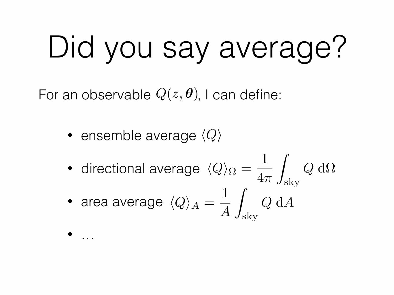
Did you say average?For an observable , I can define: Q(z,✓)

hQi• ensemble average

• directional average

• area average

• …

hQiA =1

A

Z

skyQ dA

hQi⌦ =1

4⇡

Z

skyQ d⌦

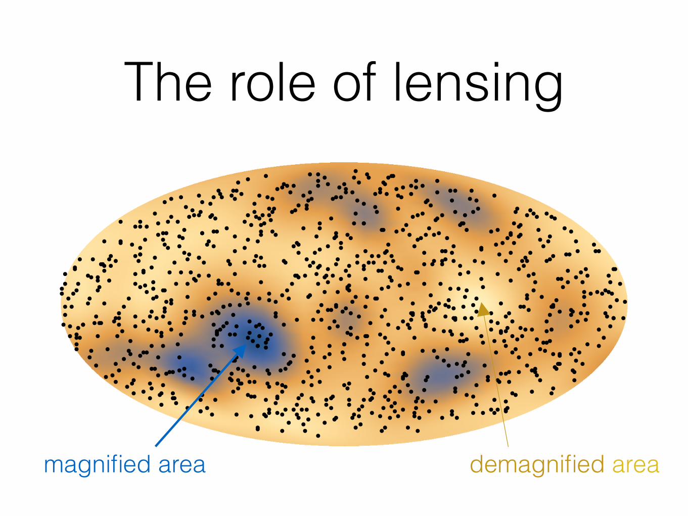
The role of lensing

magnified area demagnified area

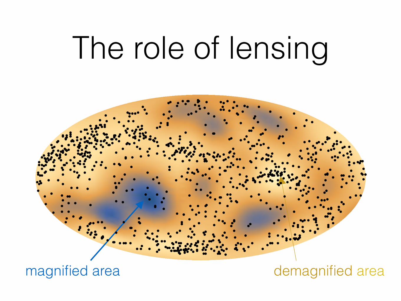
The role of lensing

magnified area demagnified area

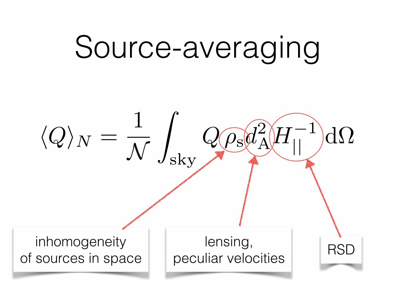
Source-averaging

inhomogeneity of sources in space

lensing, peculiar velocities RSD

hQiN =1

N

Z

skyQ ⇢sd

2AH

�1|| d⌦

Peculiar velocities

observer while R2

has the opposite. Because peculiar velocities add to the Hubble flow,this means that R

1

is actually farther than R2

, dA

(R1

) > dA

(R2

), and thus correspondsto a larger area A

1

> A2

, where potentially more sources are present. This phenomenonis sometimes called “Doppler lensing”, and its cross-correlation with galaxy numbercounts has recently been suggested as a novel cosmological observable [86].

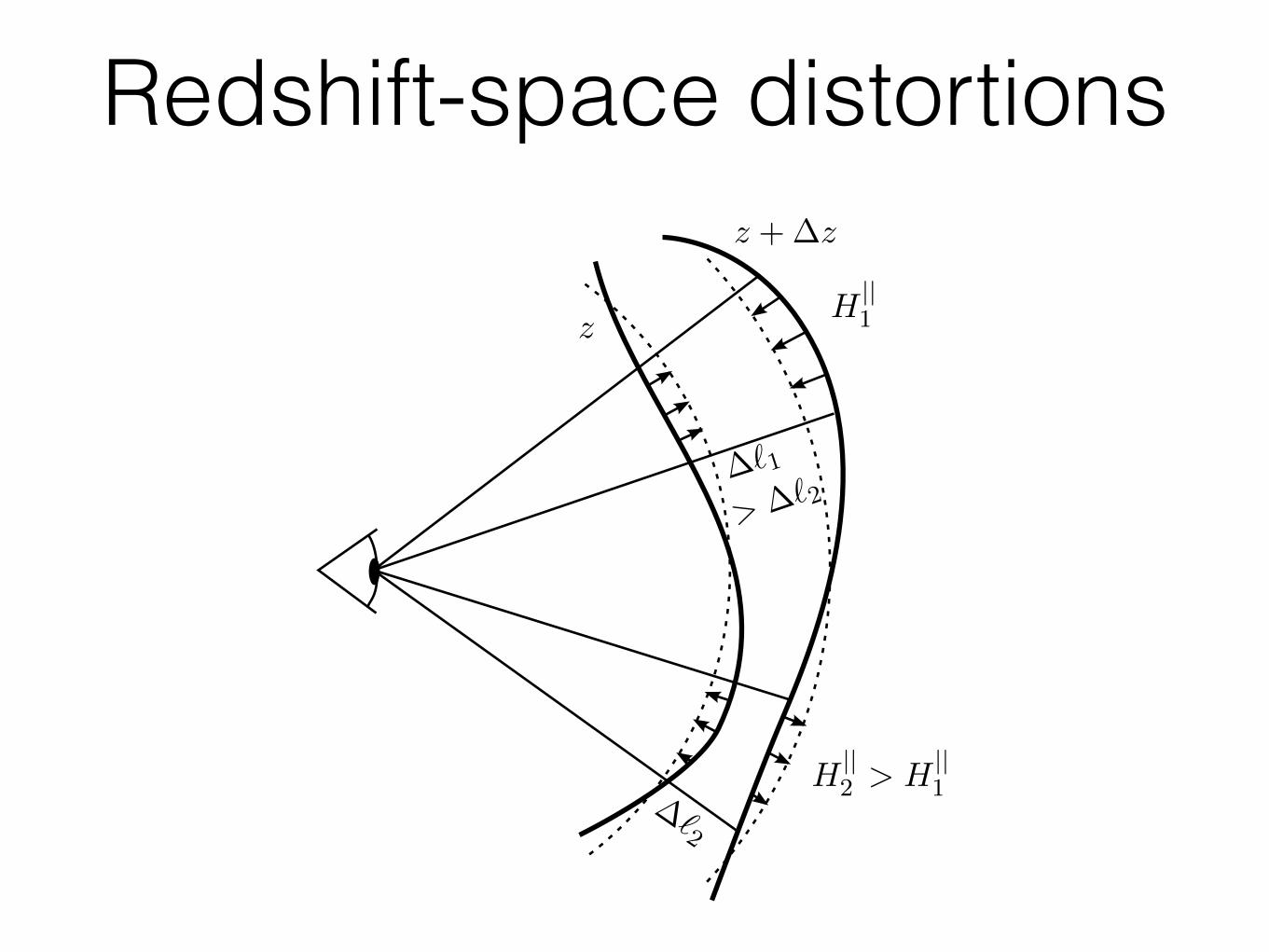
Redshift-space distortions. The physical phenomena a↵ecting redshifts have also an im-pact, via their longitudinal gradient, on the conversion between the redshift width of abin and the corresponding physical depth. This is illustrated in Fig. 4 in the case ofpeculiar velocities: a faster longitudinal expansion H|| implies a larger ratio between theredshift separation �z and distance separation �` of sources. Note that all the othercorrections to the redshift (SW, ISW, . . . ) are also accounted for by H||, because thislocal expansion is defined with respect to the rest frame of the sources, a coordinatesystem for which any e↵ect on the redshift is seen as a velocity.

⌦

z=cst

A1

> A2

A2

H||1

H||2

> H||1

�`1

�2̀

z

z +�z

> �`2

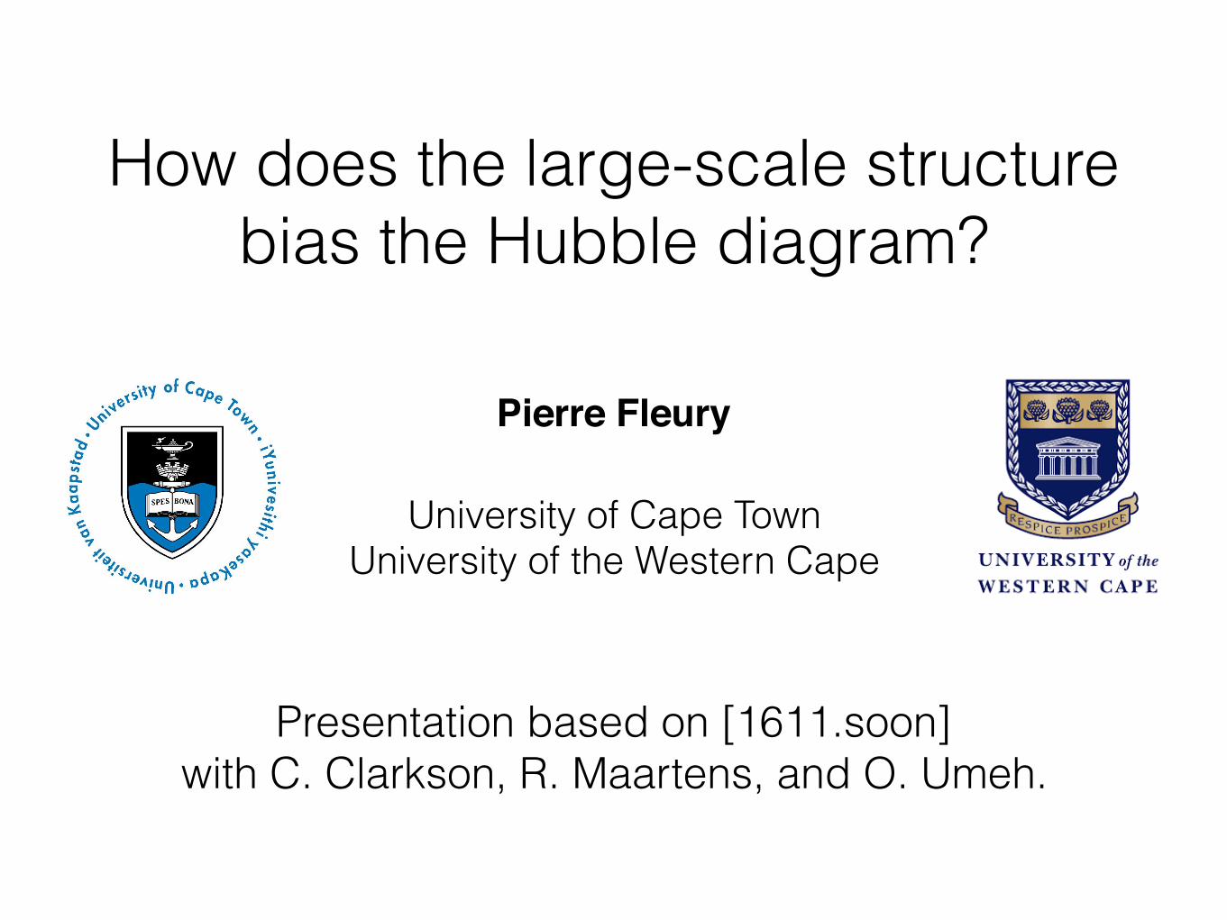
Figure 4: E↵ect of peculiar velocities on the relation between redshift space and physicalspace. Left panel : e↵ect of peculiar velocities on the geometry of an iso-z surface in physicalspace (thick solid line). The dotted line corresponds to an iso-D surface with respect to theobserver, or equivalently to the iso-z surface in a FLRW model. Right panel : idem but fortwo iso-z surfaces, illustrating the relation between the local longitudinal expansion rate H||and the physical thickness �` of a redshift bin �z.

Finally, it is important emphasise the assumed conditions under which the expres-sion (2.12) for hD(z)iN to match the best-fit D⇤(z) of an experimental Hubble diagram.

Unbiased uncertainties. In eq. (2.6) we did not take into account the fact that each datapoint (zi, Di) is weighted by the inverse square of its uncertainty 1/�2

i . This is justifiedif � is a function of z only, which is not necessarily the case. We however still recovereq. (2.6) if the uncertainties are unbiased, i.e. if they do not favour deviations of Dtowards particular a particular direction. Astrophysical phenomena are likely to producesuch a bias.

– 8 –

Redshift-space distortions

observer while R2

has the opposite. Because peculiar velocities add to the Hubble flow,this means that R

1

is actually farther than R2

, dA

(R1

) > dA

(R2

), and thus correspondsto a larger area A

1

> A2

, where potentially more sources are present. This phenomenonis sometimes called “Doppler lensing”, and its cross-correlation with galaxy numbercounts has recently been suggested as a novel cosmological observable [86].

Redshift-space distortions. The physical phenomena a↵ecting redshifts have also an im-pact, via their longitudinal gradient, on the conversion between the redshift width of abin and the corresponding physical depth. This is illustrated in Fig. 4 in the case ofpeculiar velocities: a faster longitudinal expansion H|| implies a larger ratio between theredshift separation �z and distance separation �` of sources. Note that all the othercorrections to the redshift (SW, ISW, . . . ) are also accounted for by H||, because thislocal expansion is defined with respect to the rest frame of the sources, a coordinatesystem for which any e↵ect on the redshift is seen as a velocity.

⌦

z=cst

A1

> A2

A2

H||1

H||2

> H||1

�`1

�2̀

z

z +�z

> �`2

Figure 4: E↵ect of peculiar velocities on the relation between redshift space and physicalspace. Left panel : e↵ect of peculiar velocities on the geometry of an iso-z surface in physicalspace (thick solid line). The dotted line corresponds to an iso-D surface with respect to theobserver, or equivalently to the iso-z surface in a FLRW model. Right panel : idem but fortwo iso-z surfaces, illustrating the relation between the local longitudinal expansion rate H||and the physical thickness �` of a redshift bin �z.

Finally, it is important emphasise the assumed conditions under which the expres-sion (2.12) for hD(z)iN to match the best-fit D⇤(z) of an experimental Hubble diagram.

Unbiased uncertainties. In eq. (2.6) we did not take into account the fact that each datapoint (zi, Di) is weighted by the inverse square of its uncertainty 1/�2

i . This is justifiedif � is a function of z only, which is not necessarily the case. We however still recovereq. (2.6) if the uncertainties are unbiased, i.e. if they do not favour deviations of Dtowards particular a particular direction. Astrophysical phenomena are likely to producesuch a bias.

– 8 –

Bias of distance observables

Comprehensive and balanced sky coverage. The fact that h· · ·iN involves an integralover the whole sky implicitly assumes that the survey to which it is compared alsocovers the whole sky, instead of focusing on a given region as it is currently the case formost SN surveys [6]. In the latter situation, one has to multiply the integration kernelby (d⌧

obs

/d⌦)(✓), representing the fraction of observation time spent in the direction ✓.

Large number of sources. The transition (2.8) from a discrete sum to an integral requiresto have a large number of sources, so that the sky can be safely divided into smallenough patches where the distance-redshift can be considered mostly homogeneous. Theimpact of increasing the size of such patches can be observed in Fig. 5 of ref. [87].

3 Bias of distance observables

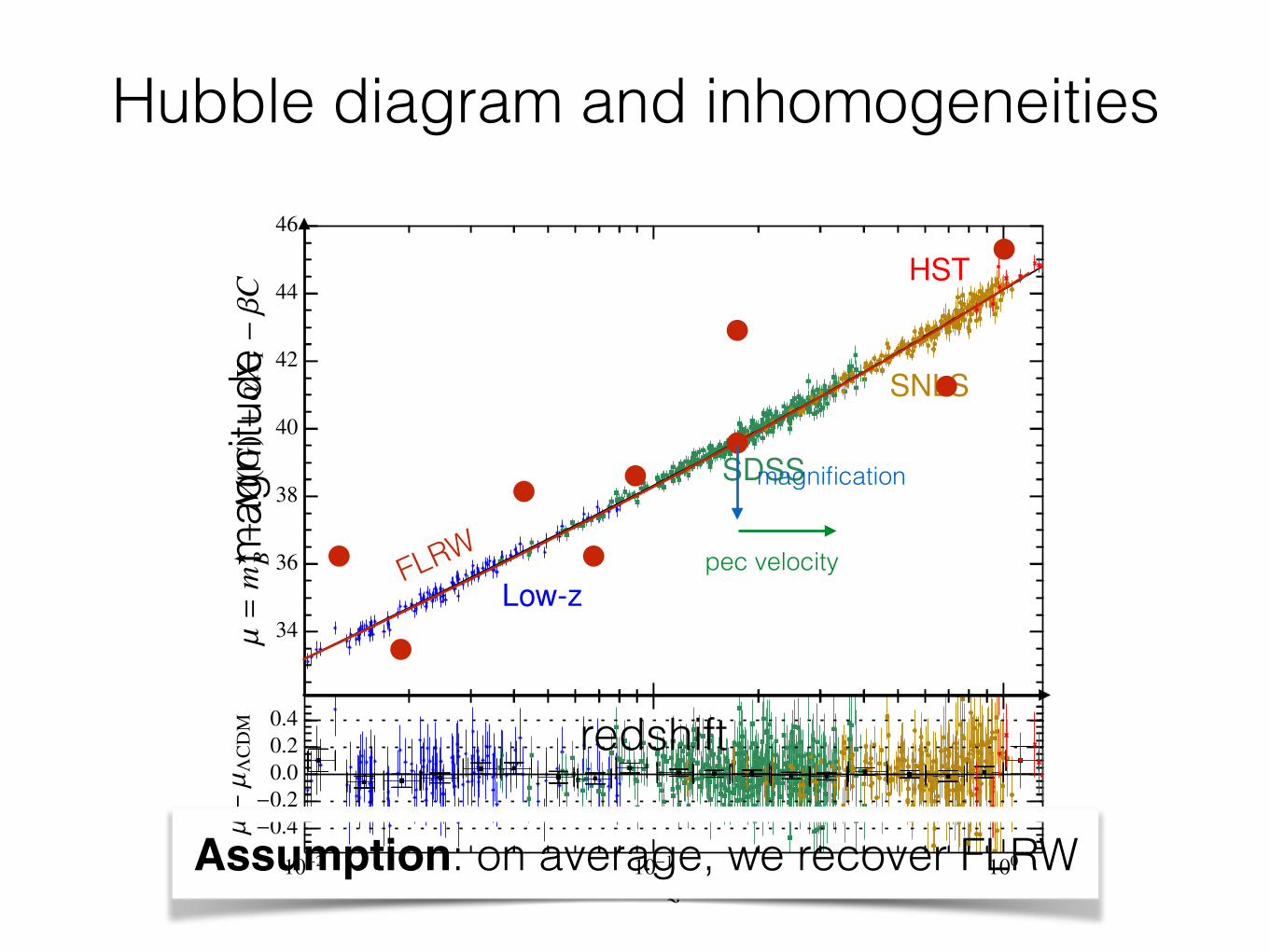
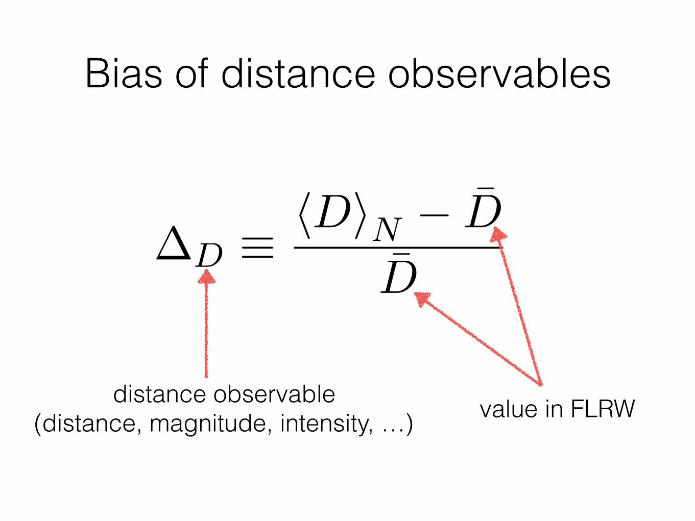
This section is dedicated to the computation of the bias of source-averaged distance indi-cators hDiN at second order in cosmological perturbations. We remind the reader that Dcan stand for angular or luminosity distance, luminous intensity (sometimes called flux), ormagnitude. What we call bias here is the di↵erence between hD(z)iN , i.e. the observedaverage distance-redshift relation, and the standard D̄(z) predicted by an unperturbed FLRWmodel with the same cosmological parameters. In other words, such a bias quantifies the errorthat one makes when fitting the Hubble diagram with the standard relation D̄(z).

In what follows, we will always consider the fractional bias defined as

�D ⌘ hDiN � D̄

D̄=

⌧D � D̄

D̄

�

N

⌘ h�DiN , (3.1)

except when D represents the magnitude m, which is already a logarithmic quantity, so thatwe rather use �m ⌘ m� m̄ and �m ⌘ h�miN in that case. Furthermore, because we do notknow what is the actual spacetime geometry of the Universe but only its statistical properties,the only quantity that we can predict is the ensemble average h�Di of �D, i.e. its averageover multiple realisation of the Universe. Note that, as extensively discussed in ref. [84], it iscrucial to take this ensemble average after source-averaging, since they do not commute ingeneral.

3.1 Calculation at second order

3.1.1 Preliminaries

We aim at using the results of ref. [77, 78], which provided a comprehensive analysis of lightpropagation up to second order in cosmological perturbations, and determined the expressionof the angular distance-redshift relation d

A

(z) at that order. The first step therefore consistsin expressing �D in terms of this result. We thus consider D a function of the angulardistance d

A

, so that, expanding D(d̄A

+ �dA

) at second order yields

�D = ↵�dA

+ �(�dA

)2 (3.2)

with

↵ ⌘ d̄A

D̄

dD

ddA

and � ⌘ 1

2

d̄2A

D̄

d2D

ddA

2

, (3.3)

except, again, when D = m in which case eq. (3.2) still holds but with slightly di↵erentdefinitions for ↵ and � (remove D̄). Table 1 lists the values of ↵ and � associated with themost commonly used distance indicators.

– 9 –

distance observable (distance, magnitude, intensity, …) value in FLRW

Bias of distance observables

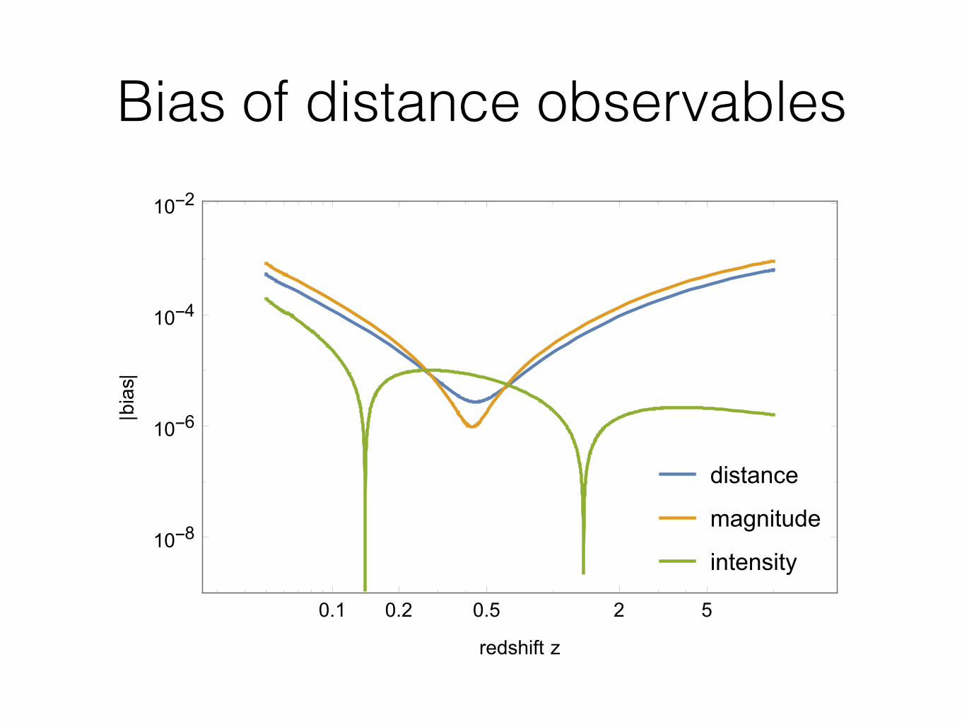
distance

magnitude

intensity

0.1 0.2 0.5 2 5

10-8

10-6

10-4

10-2

redshift z

|bias|

Effective DE EoS

w(z)• In FLRW, the dark-energy equation of state influences the relation

• If you interpret a biased Hubble diagram with FLRW, the bias can translate into a spurious

D(z)

we↵(z)

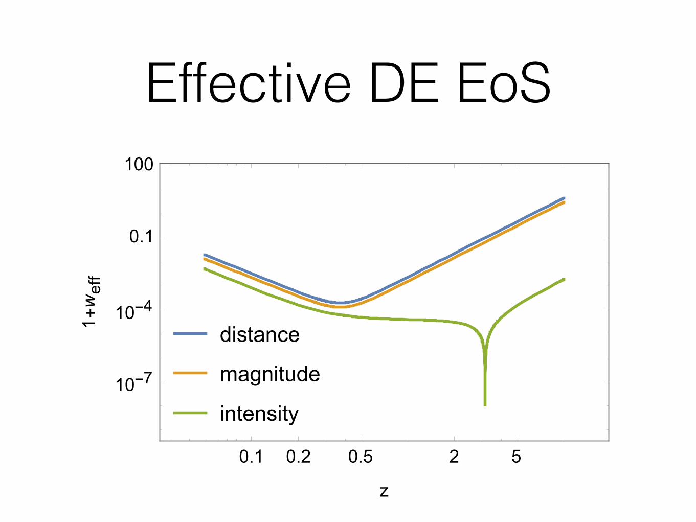
Effective DE EoS

distance

magnitude

intensity

0.1 0.2 0.5 2 5

10-7

10-4

0.1

100

z

1+weff

Question

How is the measurement of cosmological parameters influenced?

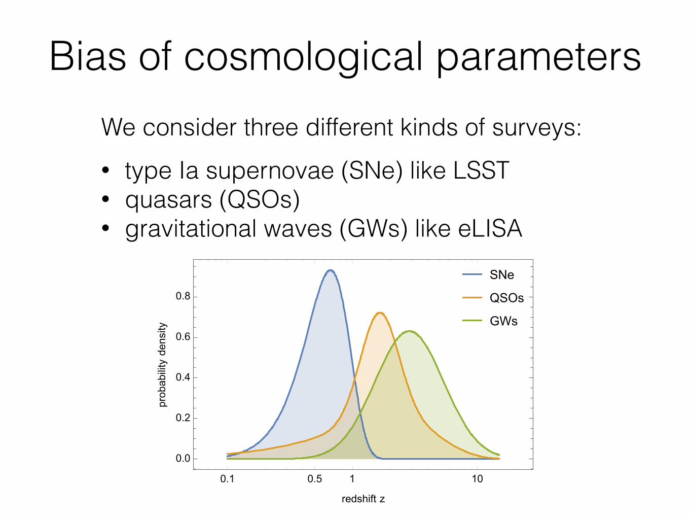
Bias of cosmological parametersWe consider three different kinds of surveys: • type Ia supernovae (SNe) like LSST • quasars (QSOs) • gravitational waves (GWs) like eLISA

SNe

QSOs

GWs

0.1 0.5 1 10

0.0

0.2

0.4

0.6

0.8

redshift z

probabilitydensity

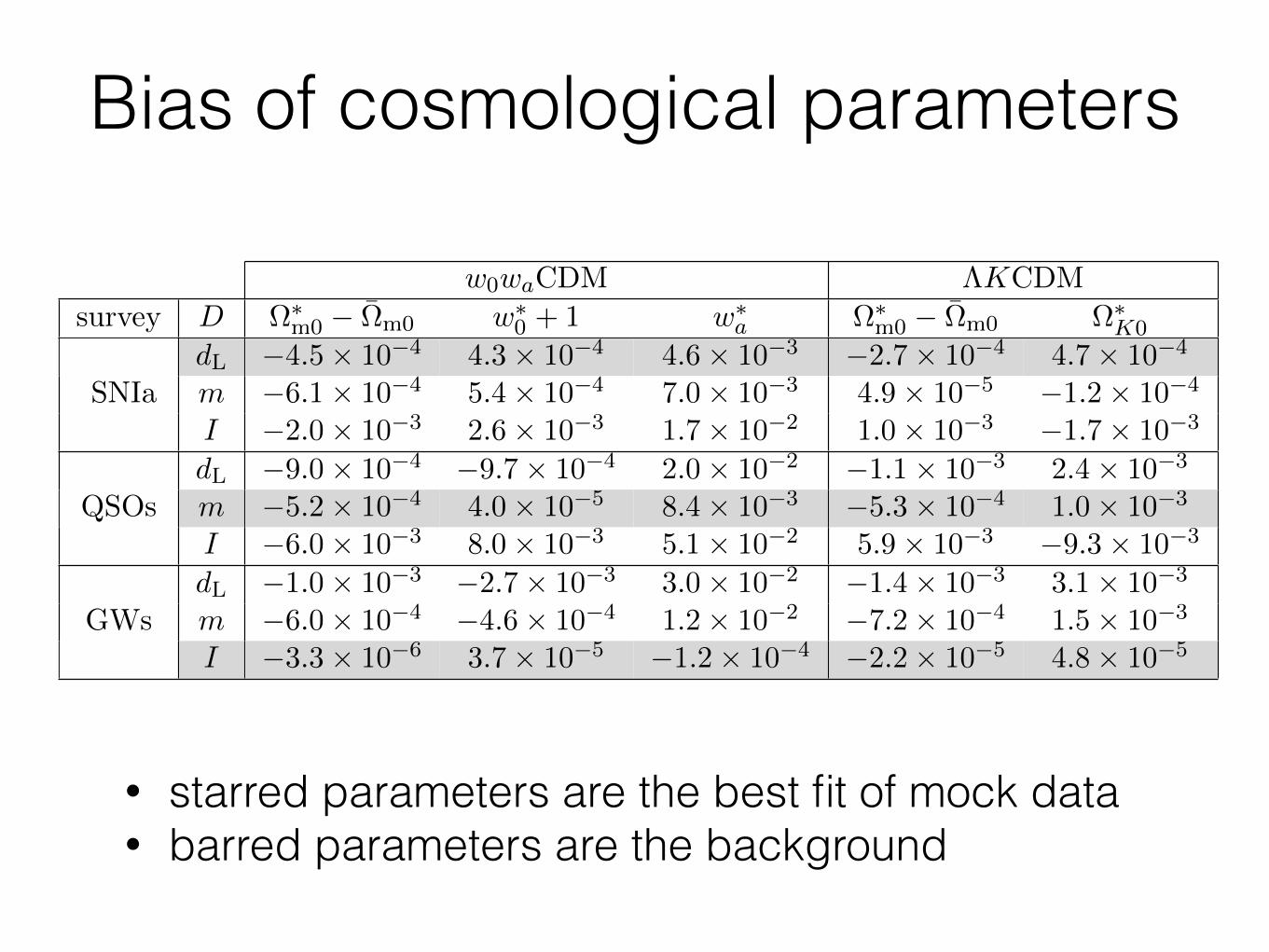
Bias of cosmological parameters

w0

waCDM ⇤KCDMsurvey D ⌦⇤

m0

� ⌦̄m0

w⇤0

+ 1 w⇤a ⌦⇤

m0

� ⌦̄m0

⌦⇤K0

SNIadL

�4.5⇥ 10�4 4.3⇥ 10�4 4.6⇥ 10�3 �2.7⇥ 10�4 4.7⇥ 10�4

m �6.1⇥ 10�4 5.4⇥ 10�4 7.0⇥ 10�3 4.9⇥ 10�5 �1.2⇥ 10�4

I �2.0⇥ 10�3 2.6⇥ 10�3 1.7⇥ 10�2 1.0⇥ 10�3 �1.7⇥ 10�3

dL

�9.0⇥ 10�4 �9.7⇥ 10�4 2.0⇥ 10�2 �1.1⇥ 10�3 2.4⇥ 10�3

QSOs m �5.2⇥ 10�4 4.0⇥ 10�5 8.4⇥ 10�3 �5.3⇥ 10�4 1.0⇥ 10�3

I �6.0⇥ 10�3 8.0⇥ 10�3 5.1⇥ 10�2 5.9⇥ 10�3 �9.3⇥ 10�3

GWsdL

�1.0⇥ 10�3 �2.7⇥ 10�3 3.0⇥ 10�2 �1.4⇥ 10�3 3.1⇥ 10�3

m �6.0⇥ 10�4 �4.6⇥ 10�4 1.2⇥ 10�2 �7.2⇥ 10�4 1.5⇥ 10�3

I �3.3⇥ 10�6 3.7⇥ 10�5 �1.2⇥ 10�4 �2.2⇥ 10�5 4.8⇥ 10�5

Table 2: Cosmological parameters ⌦⇤ fitted from a biased Hubble diagram D(z), dependingon the distance indicator D (luminosity distance d

L

, magnitude m, or intensity I), for threedi↵erent kinds of survey (SNIa, QSOs, GWs), and with two di↵erent cosmological models(w

0

waCDM or ⇤KCDM). We highlighted the least biased distance indicator for each survey.

equation of state can have order-unity departures from w = �1 at high redshift. This apparentdiscrepancy can be understood by noticing that it is impossible to reproduce the redshiftevolution of w

e↵

as seen in Fig. 7 with the parametrisation of eq. (4.10).It is interesting to note that each survey has a di↵erent least biased distance indicator:

luminosity distance for SNIa, magnitude for QSOs (although the di↵erence between distanceand magnitude is very small) and intensity for GWs. It is easy to understand this resultby comparing �D(z) of Fig. 6 with the survey’s redshift distributions p(z) of Fig. 8. Thedistributions of both SNIa and QSOs peak around z = 0.5 � 1, which is contained in thesmall window where |�I | > |�d

A

|, |�m|. On the contrary, the GW distribution peaks atmuch higher redshift, where |�I | < |�d

A

|, |�m| as it is free from gravitational lensing. It wastherefore expected that the biases weighted by the redshift distributions would lead to suchresults.

4.3 How to remove the bias in practice?

Even though this bias of the Hubble diagram due to cosmological perturbations turns out tobe relatively small, it is still a systematic e↵ect that will eventually need to be corrected as theprecision of observations increases. There are in practice two possibilities to get rid of the bias.The brute-force idea consists in calculating it for each distance indicator and systematicallysubtracting it from the observations. This may require to establish fitting formulae for �D

for any set of cosmological parameters, in order to improve computing e�ciency.Another approach, approximate but completely free and less model-dependent, consists

in choosing the right distance indicator to plot and fit the Hubble diagram at hand. As wecan see from table 2, in the case of GW choosing to fit I instead of d

L

allows one reducethe bias by two orders of magnitude, which is a significant gain. More clever choices of thequantities ↵,� can further reduce the bias if needed.

5 Conclusion

In this article, we have investigated how the inhomogeneity of the Universe, modelled by thecosmological perturbation theory, biases the distance-redshift relation probed by the Hubble

– 17 –

• starred parameters are the best fit of mock data • barred parameters are the background

Conclusions• When interpreting data, be careful with the notion

of average that you use

• The bias of the Hubble diagram due to inhomogeneities is smaller than

• The impact on parameter inference is small…

• …but it must absolutely be taken into account for direct measurements of

10�3

w(z)

Thanks Ngiyabonga