How Do Wage Shocks Affect the Labor Supplies of Married

Couples? -Evidence from the Collective Model

Sisi Zhang∗

September 2, 2008

Abstract

This paper examines the link between income volatility and householddecision. I develop a collective model to study how married couples insureagainst each other’s permanent and transitory wage shocks by making jointlabor supply decision. Estimation using SIPP 2001 panel provides someevidence on household insurance. Couples insure against both permanentand transitory wage shocks via household labor supply, while labor responseis larger to the shocks which are permanent. There is little evidence ofinsurance by labor supply for liquidity constrained households, and littleevidence of insurance against high individual wage volatility.

JEL Codes: D12, D13, D81, J22.Keywords: Collective Labor Supply, Permanent Shocks, Transitory

Shocks, Intra-household Allocation, Household Insurance.

∗Department of Economics, Boston College, 140 Commonwealth Ave, Chestnut Hill, MA,02467. Email: zhangse@bc.edu. I am especially grateful to Peter Gottschalk and Shannon Seitzfor invaluable advice. I would also like to thank Susanto Basu, Kit Baum, Kathy Bradbury,Donald Cox, Arthur Lewbel, John Knowles, Jeffery Smith, Bradley Wilson, Bo Zhao, the par-ticipants at SOLE 2008 Annual Meeting poster session, ZEW Workshop on “Gender and theLabour Market” (2008), EEA Annual Meeting (2008), 41st Annual Meeting of the CanadianEconomic Association (2007), International Symposium on Contemporary Labor Economics atXiamen University (2007), seminar participants at the Federal Reserve Bank of Boston for helpfulcomments. I benefit from financial support of CSWEP summer fellowship (2007) from FederalReserve Bank of Boston and Dissertation Fellowship (2007, 2008) from Boston College. Theusual disclaimer applies.

1

1 Introduction

There have been extensive studies that document the significant increase in earn-

ings and household income volatility in the last couple decades (Moffitt and Gottschalk

2008, Haider 2001, Hacker 2006). Such increase in income volatility have been of

concern to policy makers since it is associated with increase in risk and reduction in

welfare. Government insurance programs such as social security or unemployment

benefit help to buffer the welfare loss caused by income volatility. Meanwhile, in-

dividuals who live in the same household could also provide insurance against each

other’s adverse shocks by making joint decisions such as labor supply decision, self-

insurance, durable goods replacement, etc. The goal of this paper is to examine

the link between rising income volatility and household joint labor supply decision.

In particular, this paper looks at whether and how married couples make joint la-

bor supply decisions and intra-household allocations in response to each other’s

permanent and transitory wage shocks. The answer to this question matters for

the following reasons: First, it provides a better understanding of intra-household

insurance in reaction to rising income volatility. Second, if permanent shocks and

transitory shocks do have different impacts on labor supply, public policies that

target on shocks of different durability would have different implications. Third,

the presence of mechanisms that allow households to smooth individual shocks

also has implications on aggregate results such as the link between individual in-

come volatility and household income volatility, or the shifts in the consumption

distribution and income distribution.

Studies on insurance to income shocks has a long history in both macroeco-

nomics and labor economics. In macroeconomic theory, complete market hypoth-

esis assumes that consumption is fully insured against both permanent and transi-

2

tory income shocks. This hypothesis is usually rejected using micro data (Cochrane

1991, Altonji et al. 1992, Townsend 1994). On the other hand, permanent income

hypothesis assumes that consumption depends primarily on permanent income,

since consumers use saving and borrowing to smooth consumption in response to

transitory changes in income. Empirical studies using both aggregate and mi-

cro data show consumption reacts too little to permanent shocks (Attanasio and

Pavoni 2006) or excess sensitive to transitory shocks (Hall and Mishkin 1982). Re-

cent studies by Blundell et al. (2008) do not impose any priori on which of the

above hypothesis is true but allow for partial insurance and estimate the degree

of insurance against permanent or transitory income shocks. Using panel data in

income and imputed non-durable consumption, they find some partial insurance of

permanent income shocks and little evidence against full insurance for transitory

income shocks.

Studies on insurance against income shocks in labor economics mostly focus on

labor supply decision and also find mixed evidence. The “Added Worker Effect”

literature examines temporary change in wives’ labor supply (hours worked or par-

ticipation) in response to husbands’ unemployment or transitory earnings shocks.

Lundberg (1985) has found a small but significant added worker effect from the

Seattle and Denver Income Maintenance Experiments. Juhn and Potter (2007)

use matched March CPS files and find that added worker effect is still important

among a subset of couples but the overall value of marriage as a risk-sharing ar-

rangement has diminished due to the greater positive co-movement of employment

within couples. Garcia-Escribano (2004) finds that the smoothing resulting from

the wives’ labor response is larger for households with limited access to credit

using Panel Study of Income Dynamics (PSID). Most of these studies focus on

wives’ response to husbands’ shocks and mainly unemployment shocks. Yet little

3

is known about how husbands respond to wives’ income shocks at the same time

and whether the response would be different for permanent and transitory shocks.

This paper investigates household insurance via labor supply theoretically and

empirically. I build a theory based on the collective framework first developed by

Chiappori (1988). Such a model starts from a basic assumption that household

members jointly make Pareto efficient decisions. The unobserved intra-household

allocation (sharing rule) can be recovered from the observations of labor supply.

In this paper I allow this sharing rule to depend on permanent and transitory wage

shocks of each agent. It is important to distinguish shocks of different durability

because they are determined by different economic factors thus may have different

policy implications. For instance, the permanent shocks is mainly determined by

changes in skill prices and transitory shocks are usually caused by job instability,

unexpected illness, etc. Another advantage of this model is it does not impose

any priori on how shocks should affect household labor supply. Estimation of this

sharing rule uncovers to what extent joint labor supply insure against husbands

and wives’ wage shocks, both permanent and transitory. I also allow the sharing

rule to switch when one of the partners is not working. The comparison of sharing

rules across employment status sheds light on how couples share resources and

risks when there are unemployment shocks in addition to wage shocks.

Most collective models are static and uses (repeated) cross-sectional data. Maz-

zocco (2004, 2005, 2007) develops a series of intertemporal collective model but

without endogenous labor supply. As permanent shocks are measurement of long-

run wage changes, I extend existing static collective model to a simple dynamic

collective model with labor supply. I make an assumption that savings decision is

made ex-ante according to expectation of future shocks, while labor supply deci-

sion is made ex-post after shocks are realized. Blundell and Walker (1986) proved

4

that by separating savings and labor supply decision into two stages, the second

stage problem only involves within-period leisure and consumption decision taken

first stage intertemporal savings decision as given. This separation between savings

and labor supply decision allows me to directly apply the theory of static collective

labor supply with nonparticipation into the second stage of my dynamic model.

This paper is closely related to the studies on insurance to income shocks, added

worker effect, collective models, and makes the following contributions to exist-

ing literature: First, I build a simple dynamic collective model to study whether

and how household labor supply insure against wage shocks. I allow permanent

shocks and transitory shocks from both husbands and wives to affect labor sup-

ply differently, but do not specify any priori such as full-insurance assumption.

Second, I examine how insurance mechanism changes when one of the partner is

not working. Third, this paper also contributes to empirical collective models by

introducing wage shocks into the sharing rules and first estimating collective labor

supply model both on extensive and intensive margin using U.S. panel data.1

Section 2 presents some stylized facts on income volatility which suggests some

evidence of household insurance via labor supply. In Section 3 I formulate a collec-

tive model that allows for insurance against permanent and transitory shocks and

discuss identification strategy for recovering unobserved sharing rule from observed

labor supply and participation. Section 4 first describes data, then I estimate per-

manent and transitory wage shocks for each individual, and estimate household

labor supply using a regime switching regression and recover sharing rules. Esti-

mation results from high frequency panel data Survey and Income Program Partic-

ipation (SIPP) provide some evidence on household insurance: Couples make joint

1Bloemen (2004) estimate Donni (2003)’s model using Dutch data. Hourriez (2005) estimateDonni (2003)’s model with French data, and only considers female nonparticipation. Vermeulen(2005) estimates discrete choice model for female labor supply with nonparticipation.

5

labor supply decisions and intra-household allocations to insure against both per-

manent and transitory wage shocks, while labor response is larger for permanent

shocks. When the husband is not working, sharing rule changes significantly and

no longer reflects household insurance. There is little evidence of insurance within

liquidity constrained households, and no evidence of insure against high individual

wage volatility. Section 5 concludes.

2 Stylized Facts of Income Volatility and House-

hold Insurance

This section presents the stylized facts of household income volatility and indi-

vidual income volatility. The comparison between income volatility at household

level and individual level and the comparison of household income volatility be-

tween married couples and single individuals suggest some evidence of insurance

against income shocks through household labor supply, which motivates this paper.

Figure 1 compares household earnings volatility with individual earnings volatil-

ity for married households, using PSID 1982-2002.2 I measure earnings volatility

as the variance of transitory component of earnings using Moffitt and Gottschalk

(2008)’s error components model.3 Over the past twenty years household earnings

volatility is always lower than either male or female earnings volatility, which sug-

gests married couples may insure each other against individual earnings volatility

so that income fluctuations at household level are lower. Since earnings depend

on wage and hours worked, labor supply as an insurance mechanism is a plausible

2I focus on labor earnings instead of total income to avoid the issue that some joint assetincome or transfers may not be assigned to individuals properly.

3Let yit = αtµi + νit where νit is transitory component for income or earnings following anARMA(1,1)process.

6

explanation to this figure.

If there exists insurance in multi-person households, then married couples would

behave differently than single individuals. Table 1 compares income volatility for

singles versus married couples using SIPP 2001 panel, the primary data source

in this paper.4 If married couples can insure each other against income shocks,

then their income fluctuation at household level should be smaller than singles

who can not provide such insurance. Since household income for married couples

is the sum of two person individual income, to make it comparable, I calculate

household income volatility for singles by randomly matching single males and

single females and sum up each two agents’ income to get “household income” or

“household earnings”. These random matched individuals do not have household

smoothing behavior while married couples might have. The first two rows of Ta-

ble 1 compares randomly matched singles with married couples household income

or household earnings volatility, married couples have much lower volatility than

randomly matched single individuals (0.141 v.s. 0.092, and 0.135 v.s. 0.085 re-

spectively). However, this may because married couples have lower wage or hours

fluctuations which are the primary component of household income. The bottom

rows shows that on the opposite, married couples actually have higher wage and

hours fluctuations.5 This finding is consistent with the hypothesis that married

couples not only adjust labor supply in response to their own wage shocks, but

also adjust labor supply in response to spouse’s wage shocks.

In short, from PSID and SIPP, two most comprehensive panel data in the

United States, evidence shows that income volatility at household level are much

4Table 1 applies method in Gottschalk and Moffitt (1994), which uses entire sample pe-riod(three years) to compute a single variance. I measure transitory income fluctuations bycalculating variances for each household over time, then take the average across all households.I use the same sample cuts as in estimation section.

5I take logarithm thus the statistics does not include those who do not work.

7

smaller than at individual level for married couples, and married couples have lower

household income volatility than single individuals. These stylized facts suggest

some evidence of household insurance through labor supply, which the following

sections provide both theoretical and empirical investigation.

3 Model

I build theory based on collective models developed by Chiappori (1988), Maz-

zocco (2004) and Donni(2003). Household members jointly make ex-ante savings

decision and ex-post labor supply decision to maximize a weighted sum of indi-

vidual utility function over life-cycle. The unobserved intra-household allocation

mechanism (sharing rule) depends on husbands’ and wives’ permanent wage shocks

and transitory wage shocks, and this sharing rule can be identified from observed

labor supply and participation decision up to a constant. This model provides a

framework to examine how household make joint labor supply decision in respond

to each other’s permanent and transitory wage shocks.

3.1 Basic Setting

3.1.1 Preferences and Household Problem

Consider a two-member household consisting of a husband (m) and a wife (f).

Let hfit and hmit denote f and m’s labor supply between 0 and 1 for household i

in period t. Let cfit and cmit denote f and m’s individual consumption of a private

Hicksian commodity. The price of the consumption good is set to 1. Assume no

home production so that leisure and labor supply sum up to 1.6 Assume individual

6Most empirical studies using collective model make this assumption because most data arelack of information on home production.

8

preferences are “egoistic”, so that utilities can be written as U jit(1 − h

jit, c

jit) (j =

f,m), where U jit is continuously differentiable, strictly monotone, strictly quasi-

concave and intertemporal additive separable over life-cycle.7 Let wfit and wmit

denote f and m’s stochastic wage rate in period t respectively. Let yit denotes

non-labor income, which includes asset income and transfers and Ait denotes net

wealth in period t−1. Household decision process is assumed to be Pareto efficient,

which is the main assumption for collective models, and this implies agents fully

commit to the future allocations of resources. The Pareto problem is to choose

labor supply, consumption and savings to maximize discounted weighted utilities

of two agents over life-cycle:

maxhf

it,cfit,h

mit ,c

mit ,Ai,t+1

E0[T∑t=1

βt−1(µitUfit(1− h

fit, c

fit) + Um

it (1− hmit , cmit ))]

s.t.cfit + cmit + Ai,t+1 ≤ wfithfit + wmit h

mit + yit + Ait ∀t

wfit = wfit + δfit + νfit, wmit = wmit + δmit + νmit

(1)

where the non-negative scalar µit defines the wife’s Pareto weight, which could

depend on both agents’ wage, non-labor income and some distribution factors that

affect outside environment of the household (Chiappori et al. 2002).8 Since wages

are stochastic, I allow µit to depend on both fixed component of wage wfit and wmit ,

as well as stochastic shocks: permanent shocks δfit, δmit and transitory shocks νfit, ν

mit .

Underlying the function µit is some intra-household resource allocation mechanism

that leads to Pareto efficient allocations.

7Chiappori (1992) show that main results for egotistic preference also hold in a more generalcase of “caring” agents, whose preferences are represented by a utility function that dependson both their egotistic utility and their spouses’. For estimation purposes, I focus on egotisticpreferences only.

8Interest income rtAit is already included in yit by definition.

9

3.1.2 Two-Stage Budgeting

Chiappori (1988) and Mazzocco (2004) have shown that under the assumption

of Pareto efficiency, according to the Second Welfare Theorem, a weighted maxi-

mization of household utility function can be decentralized given intra-household

transfers (sharing rule). By entering marriage a husband and a wife first agree

upon a sharing rule to allocate the pooled household resources, then each member

maximize his or her own utility given allocated resources.

Existing collective models are either static (Chiappori 1988, Donni 2003) or

intertemporal but without endogenous labor supply (Mazzocco 2004).9 I extend

the static collective model into a simple dynamic context by making an assumption

that household make savings decision ex-ante and labor supply decision ex-post.

Blundell and Walker (1986) showed that when preferences are intertemporally sep-

arable, decision-making under uncertainty can be viewed as a two-stage budgeting

process: in the first stage the household optimally allocates full life-cycle wealth

over each period to equalize marginal utility of money across periods, and reallo-

cate wealth according to realized shocks in previous period. In the second stage,

current period’s allocation of income net of savings is distributed between con-

sumption and leisure, thus the second stage becomes a within-period decision.10

Incorporating both collective models’ two-step decision and Blundell and Walker

(1986)’s separation between savings and labor supply, I specify a two-stage collec-

9To my knowledge, Mazzocco and Yamaguchi (2006) are the only one who develop dynamiccollective model with endogenous labor supply and participation. They consider three discretechoice of labor supply: full-time, part-time and nonparticipation while I consider continuoushours choice in this paper. They simulate a model to capture the empirical features of laborsupply, saving and marital choices. Although marital status and commitment issue affects laborsupply and savings decision, I focus on intact families only to study their joint decisions inresponse to each other’s wage shocks. Marriage decision is beyond the scope of this paper and isleft to future research.

10Their model are based on single decision maker households, but it can be applied to collectivemodels (Chiappori, Fortin and Lacroix 2002).

10

tive decision process as follows: at the beginning of marriage, a husband and a wife

optimally allocate life-cycle wealth in each period according to their expectation

to the future shocks, and commit to a sharing rule to allocate future resources

conditional on both partners’ wage shocks in each period. The second stage is

a within-period decision: once shocks are realized, the husband and the wife al-

locate non-labor income net of savings according to the sharing rule, and each

agent chooses private consumption and labor supply subject to earnings plus the

allocated non-labor income net of savings:

maxhj

it,cjit

U jit(1− h

jit, c

jit)

s.t. cjit ≤ (wjit + δjit + νjit)hjit + φjit j = f,m ∀t

φfit = φit, φmit = yit − sit − φit

(2)

where φfit is the amount of non-labor income net of savings allocated to the wife,

and φmit is the rest amount allocated to the husband.

3.1.3 Sharing Rule

Sharing rules in existing collective models depend on each agent’s wage, non-

labor income and distribution factors. This paper aims to examine how shocks

affect household joint decision and how shocks at different persistency level affect

joint decision differently. Therefore, I allow both permanent shocks and transitory

shocks of each agent to enter the sharing rule. Wage shocks not only affect labor

supply through household budget constraint but also through this sharing rule. I

specify the sharing rule as a function of husbands’ and wives’ fixed component of

wage, permanent shocks, transitory shocks, non-labor income net of savings and a

11

vector of distribution factors z:

φit = φ(yit − sit, wfit, wmit , δfit, δ

mit , ν

fit, ν

mit , zit) (3)

where sit is active savings in period t. As defined in Equation (2), φit is the

amount of non-labor income net of savings that allocates to the wife. It could be

larger than the total amount of non-labor income net of savings, in which case the

husband not only transfers all the non-labor income but also transfers part of his

own earnings to the wife. This sharing rule can also be a negative value, in which

case the wife transfers some of her earnings to the husband.

3.1.4 Identification of the Sharing Rule when Both Partners Are Work-

ing

When both partners work positive hours, the second stage problem in equation

(2) can be solved by First Order Conditions. I derive Mashallian labor supply as

a function of one’s own wage rate and the sharing rule:

hfit = hfit(wfit, φ(yit − sit, wfit, wmit , δ

fit, δ

mit , ν

fit, ν

mit , z))

hmit = hmit (wmit , yit − sit − φ(yit − sit, wfit, wmit , δ

fit, δ

mit , ν

fit, ν

mit , z))

(4)

From observed labor supply, one can identify the unobserved sharing rule up

to an additive constant (Chiappori 1988). The intuition for identification is that

changes in non-labor income and the wife’s wage and shocks only affect the hus-

band’s labor supply through the sharing rule, and vice versa. In Section 3.2 I

specify functional form for Mashallian labor supply and the sharing rule, these

structural parameters can be recovered as a function of reduced form parameters.

12

3.1.5 Identification of the Sharing Rule When One of the Parters Is

Not Working

The identification strategy described so far does not involve corner solutions. In

this paper I not only look at how couples insure each other’s wage shocks when both

of them are working, but also look at how one agent adjust labor supply when the

spouse is not working. I apply identification strategy from Donni (2003). When

one of the partners does not participate, the sharing rule switches regime from

when both partners participate. Identification comes from the characterization

of the reservation wage by “double indifference”: at the wage when one agent is

indifferent between working and not working, Pareto efficiency requires that the

spouse must be indifferent as well.11 The sharing rule when one of the partners

is not working can still be identified (up to an additive constant) from spousal

continuous labor supply.12

3.2 Specification

For estimation purposes, I specify a log-linear labor supply and a linear sharing

rule. There are two advantages of these specifications: First, linear or log-linear

function is usually assumed in the collective model with nonparticipation and un-

observed heterogeneity (Blundell et al. 2007, Bloemen 2004). Second, I can also

prove the existence of a Pareto weight which is always positive and depends on

wage shocks.

11Suppose not, if the wife is indifferent between working or not, but her participation yieldsa positive gain for her spouse, then she will choose to participate, otherwise the decision is notPareto optimal.

12When neither husband or wife works, sharing rule is not identified as there is no variationsin labor supply.

13

3.2.1 Labor Supply, Sharing Rule and Indirect Utility Functions

I specify a log-linear Mashallian labor supply functions as follows:

loghfit = α0 + α1logwfit + α2φit

loghmit = β0 + β1logwmit + β2(yit − sit − φit)(5)

The log-wage specification is consistent with Mincer model. I do not impose log-

arithm on the sharing rule since in theory it could be negative: when the wife

transfers not only all non-labor income but also some of her earnings. I choose log

hours specification to ensure the corresponding Pareto weight is consistent with

theory. One limitation of this linear functional form is the lack of flexibility since

labor supply curve is upward sloping everywhere.

Following collective literature, I specify a sharing rule as a linear function in

all its arguments and include two distribution factors:

φit = k0+k1(yit−sit)+k2wfit+k3w

mit +k4δ

fit+k5δ

mit +k6ν

fit+k7ν

mit +k8z1i+k9z2i (6)

where z1i and z2i are two distribution factors that affect spouses’ opportunities

outside marriage without affecting their preferences.13

Labor supply functions in equation (5) suggest the following indirect utility

functions, which one can perform intrahousehold welfare analysis of changes in

13The two distribution factors I choose is local sex ratio and divorce law index, both are timeinvariant in the data.

14

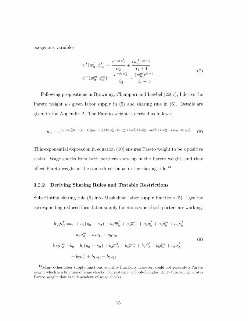
exogenous variables:

vf (wfit, φfit) =

e−α2φfit

α2

+(wfit)

α1+1

α1 + 1

vm(wmit , φmit ) =

e−β2φmit

β2

+(wmit )

β1+1

β1 + 1

(7)

Following propositions in Browning, Chiappori and Lewbel (2007), I derive the

Pareto weight µit given labor supply in (5) and sharing rule in (6). Details are

given in the Appendix A. The Paretio weight is derived as follows:

µit = eα2+β2[(k0+(k1−1)(yit−sit)+k2wfit+k3w

mit +k4δ

fit+k5δ

mit +k6ν

fit+k7ν

mit +k8z1i+k9z2i] (8)

This exponential expression in equation (10) ensures Pareto weight to be a positive

scalar. Wage shocks from both partners show up in the Pareto weight, and they

affect Pareto weight in the same direction as in the sharing rule.14

3.2.2 Deriving Sharing Rules and Testable Restrictions

Substituting sharing rule (6) into Mashallian labor supply functions (5), I get the

corresponding reduced form labor supply functions when both parters are working:

loghfit =a0 + a1(yit − sit) + a2wfit + a3w

mit + a4δ

fit + a5δ

mit + a6ν

fit

+ a7νmit + a8z1i + a9z2i

loghmit =b0 + b1(yit − sit) + b2wfit + b3w

mit + b4δ

fit + b5δ

mit + b6ν

fit

+ b7νmit + b8z1i + b9z2i

(9)

14Many other labor supply functions or utility functions, however, could not generate a Paretoweight which is a function of wage shocks. For instance, a Cobb-Douglas utility function generatesPareto weight that is independent of wage shocks.

15

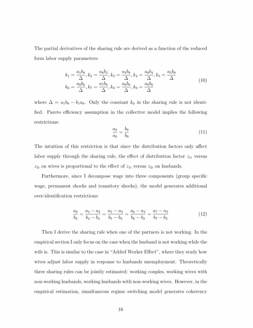
The partial derivatives of the sharing rule are derived as a function of the reduced

form labor supply parameters:

k1 =a1b8∆

, k2 =a8b2∆

, k3 =a3b8∆

, k4 =a8b4∆

, k5 =a5b8∆

k6 =a8b6∆

, k7 =a7b8∆

, k8 =a8b8∆

, k9 =a9b8∆

(10)

where ∆ = a1b8 − b1a8. Only the constant k0 in the sharing rule is not identi-

fied. Pareto efficiency assumption in the collective model implies the following

restrictions:

a8

a9

=b8b9

(11)

The intuition of this restriction is that since the distribution factors only affect

labor supply through the sharing rule, the effect of distribution factor z1i versus

z2i on wives is proportional to the effect of z1i versus z2i on husbands.

Furthermore, since I decompose wage into three components (group specific

wage, permanent shocks and transitory shocks), the model generates additional

over-identification restrictions:

a8

b8=a4 − a2

b4 − b2=a5 − a3

b5 − b3=a6 − a2

b6 − b2=a7 − a3

b7 − b3(12)

Then I derive the sharing rule when one of the partners is not working. In the

empirical section I only focus on the case when the husband is not working while the

wife is. This is similar to the case in “Added Worker Effect”, where they study how

wives adjust labor supply in response to husbands unemployment. Theoretically

three sharing rules can be jointly estimated: working couples, working wives with

non-working husbands, working husbands with non-working wives. However, in the

empirical estimation, simultaneous regime switching model generates coherency

16

problem. As Bloemen (2004) pointed out, without any further restrictions, the

double switching model may generates multiple outcomes for the participation of

husband and wife in a household. Imposing coherency in such model is either

quite complicated or greatly reduces the generality of the model. Therefore, I only

allows for one agent participation status to change.

Donni (2003) proposes a switching model for labor supply of the wife. When

the husband is not working, female labor supply switches regime:

loghfit =A0 + A1(yit − sit) + A2wfit + A3w

mit + A4δ

fit + A5δ

mit + A6ν

fit

+ A7νmit + A8z1i + A9z2i

(13)

When the husband is unemployed, the sharing rule changes because he no longer

brings income into the household and he could not adjust labor supply to insure

against the wife’s shocks either. Denote sharing rule in male nonparticipation set

as φNPit and denote parameters with upper-case:

φNPit = K0+K1(yit−sit)+K2wfit+K3w

mit+K4δ

fit+K5δ

mit +K6ν

fit+K7ν

mit +K8z1i+K9z2i

(14)

Abbreviate male labor supply function in (11) as hm = b′x, female labor supply

when the husband is working as a′x and when the husband is not working as A′x.

Donni (2003) shows the following continuity condition must hold:

A′x = a′x+ s(b′x) (15)

where s is a scalar that can be estimated. When the husband is on the participation

frontier, the last item on the right hand side disappears. The sharing rule also

17

follows a similar continuity condition:

K ′x = k′x+ q(b′x) (16)

The relation between s and q can be derived from (6), (11), (12):

q =sb8∆

(17)

Parameters K’s, which are the partial derivatives of sharing rule on male nonpar-

ticipation set, can be identified via equation (18) and (19).

3.3 Unitary Model

In previous sections I derive restrictions that labor supply functions should satisfy

under the collective setting. The alternative household decision model is called

unitary model, where household decision is made by a single agent. Household

members pool resources together and fully insure against all shocks. Consumption

is not separable into individual consumption, and household problem is represented

by a single utility function instead of weighted sum of individual utility functions.

This unitary model generates different testable restrictions. To be comparable with

collective model, I still assume ex-ante savings decision and ex-post labor supply

decision are separable in two stages. Once couples decide how much to save in the

first stage, the second stage they choose labor supply and joint consumption to

maximize a single household utility:

maxhf

it,hmit ,Cit

U(1− hfit, 1− hmit , Cit)

s.t. Cit ≤ wfithfit + wmit h

mit + yit − sit ∀t

(18)

18

Labor supply functions can still be derived as in equation (9). Slusky symmetry

implies the following restriction:

b8 = −a8 (19)

Another restriction for unitary model comes from nonparticipation. When the

husband does not work, in the collective model, his potential wage still affects the

sharing rule therefore affects labor supply, while in the unitary model, this effect

no longer exists. This implies that the effect of male potential wage on female

labor supply is zero when the husband is not working:

A3 = 0⇒ a3 + sb3 = 0 (20)

4 Data and Empirical Results

4.1 Data

This study uses Survey of Income and Program Participation (SIPP) 2001 panel,

a national representative longitudinal data set in the U.S. To study how short-

run labor supply react to wage shocks, SIPP has substantial advantage over other

panel datasets such as PSID or the Health and Retirement Study (HRS), because

SIPP interviews every other four month, while others are annual or biennial data.15

Another advantage of SIPP is that high frequency interview also gives better qual-

ity of wage data. I further use wage data purged of measurement error as in

15SIPP has monthly data but monthly data has the well-documented seam bias problem. Re-spondents are more likely to report a wage change between interviews instead of within interviewperiod.

19

Gottschalk (2005).16 Under the assumption that nominal wages adjust in discrete

steps while working for the same employer, he identifies the structural breaks in

individual wage series and separates the effect of measurement error from that of

true changes in wages.

SIPP 2001 panel consists of nine waves from December 2000 to February 2003.

The main sample cuts in the estimation include married couples with heads 20 to

59 years old. I also excludes households who have children less than 18 years old

because the model does not account for home production or public consumption

and children is a big part of it. This gives a sample of 4,749 households with 41,622

observations. All income are put into January 2000 CPI-U-RS dollars.17

The dependent variable is total number of hours of work in each wave. The

measure of wage is hourly wage rate, defined as observed hourly wage for hourly

workers or the total wage earnings divided by number of hours of work otherwise.

Household non-labor income includes property income, transfer income and other

income.

Savings variable is constructed by taking the difference between net wealth in

period t and t − 1.18 Information on net wealth is only available in the 3rd, 6th

and 9th wave in SIPP 2001 panel. I use linear interpolation to fill in for the rest

waves.19 This variable is treated as endogenous with measurement error in the

empirical section.

Following Chiappori et al. (2002), I construct two measures of distribution

16I thank Peter Gottschalk for generously providing SIPP data with his correction of mea-surement error in wage.

17The deflator can be found at http://www.census.gov/hhes/www/income/income05/cpiurs.html18I acknowledge savings constructed by this method includes both active and passive savings

while in my model only active savings is needed.19This shortcoming can not be overcome by switching to PSID data since it only has wealth

information every other five years before 1996, and biennial afterwards, and HRS data also onlyhas wealth information every other year.

20

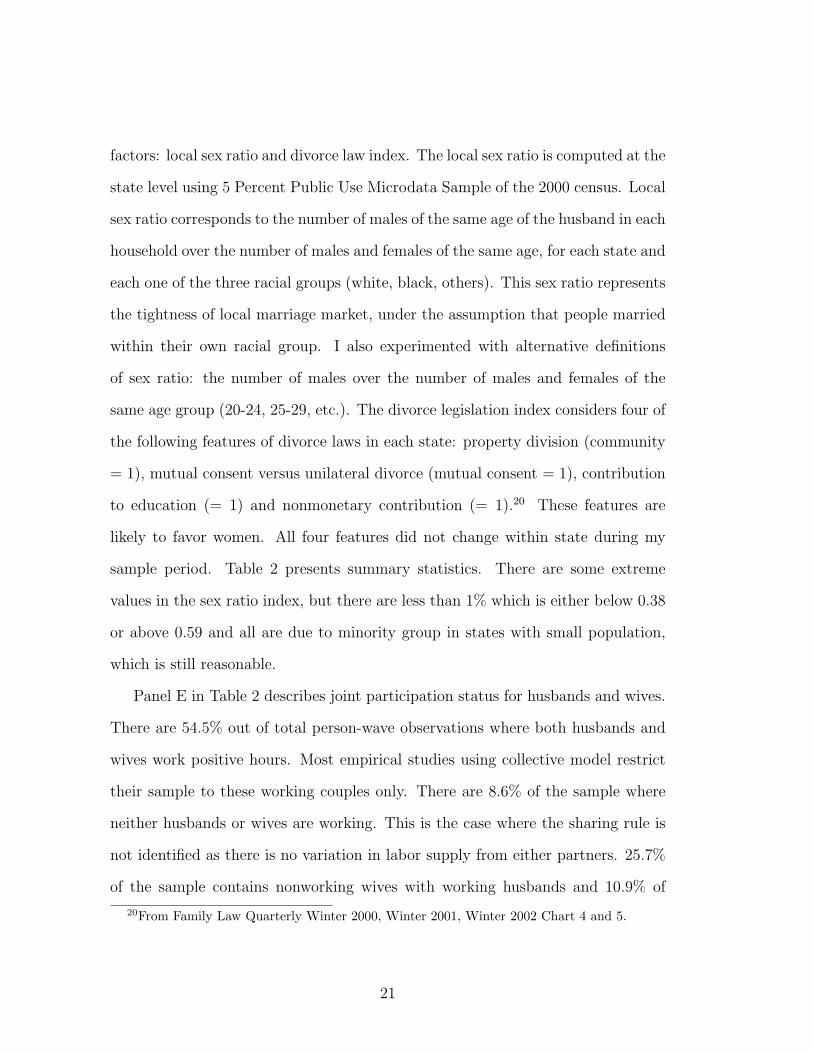
factors: local sex ratio and divorce law index. The local sex ratio is computed at the

state level using 5 Percent Public Use Microdata Sample of the 2000 census. Local

sex ratio corresponds to the number of males of the same age of the husband in each

household over the number of males and females of the same age, for each state and

each one of the three racial groups (white, black, others). This sex ratio represents

the tightness of local marriage market, under the assumption that people married

within their own racial group. I also experimented with alternative definitions

of sex ratio: the number of males over the number of males and females of the

same age group (20-24, 25-29, etc.). The divorce legislation index considers four of

the following features of divorce laws in each state: property division (community

= 1), mutual consent versus unilateral divorce (mutual consent = 1), contribution

to education (= 1) and nonmonetary contribution (= 1).20 These features are

likely to favor women. All four features did not change within state during my

sample period. Table 2 presents summary statistics. There are some extreme

values in the sex ratio index, but there are less than 1% which is either below 0.38

or above 0.59 and all are due to minority group in states with small population,

which is still reasonable.

Panel E in Table 2 describes joint participation status for husbands and wives.

There are 54.5% out of total person-wave observations where both husbands and

wives work positive hours. Most empirical studies using collective model restrict

their sample to these working couples only. There are 8.6% of the sample where

neither husbands or wives are working. This is the case where the sharing rule is

not identified as there is no variation in labor supply from either partners. 25.7%

of the sample contains nonworking wives with working husbands and 10.9% of

20From Family Law Quarterly Winter 2000, Winter 2001, Winter 2002 Chart 4 and 5.

21

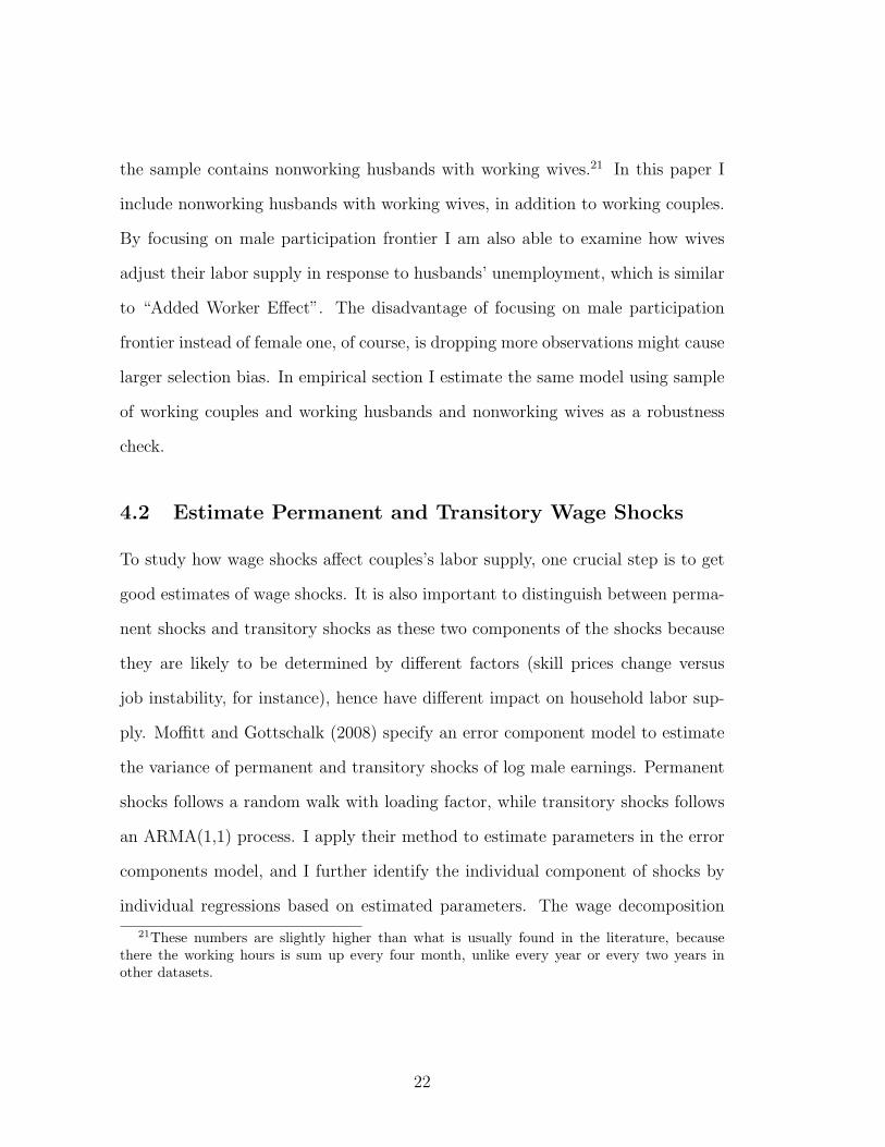
the sample contains nonworking husbands with working wives.21 In this paper I

include nonworking husbands with working wives, in addition to working couples.

By focusing on male participation frontier I am also able to examine how wives

adjust their labor supply in response to husbands’ unemployment, which is similar

to “Added Worker Effect”. The disadvantage of focusing on male participation

frontier instead of female one, of course, is dropping more observations might cause

larger selection bias. In empirical section I estimate the same model using sample

of working couples and working husbands and nonworking wives as a robustness

check.

4.2 Estimate Permanent and Transitory Wage Shocks

To study how wage shocks affect couples’s labor supply, one crucial step is to get

good estimates of wage shocks. It is also important to distinguish between perma-

nent shocks and transitory shocks as these two components of the shocks because

they are likely to be determined by different factors (skill prices change versus

job instability, for instance), hence have different impact on household labor sup-

ply. Moffitt and Gottschalk (2008) specify an error component model to estimate

the variance of permanent and transitory shocks of log male earnings. Permanent

shocks follows a random walk with loading factor, while transitory shocks follows

an ARMA(1,1) process. I apply their method to estimate parameters in the error

components model, and I further identify the individual component of shocks by

individual regressions based on estimated parameters. The wage decomposition

21These numbers are slightly higher than what is usually found in the literature, becausethere the working hours is sum up every four month, unlike every year or every two years inother datasets.

22

model is similar to Moffitt and Gottschalk (2008):

logwjiat = wjit + γjtµji + νjiat j = f,m (21)

where wjit is the group-specific wage component. γjt is loading factor on time

invariant component µi. Loading factor represents aggregate skill price changes on

human capital, it can be considered as a measure of aggregate shock. I allow this

aggregate shock to differ between men and women, thus couples can still insure

each other against this shock. Permanent shocks δmit in equation (2) come from

the product of γt and µi. νit are transitory shocks. Shocks not only move with

calendar time but also move along with age (subscript with a), so that age effect

is also taken into account.

I obtain wjit from predicted value of first stage Mincer regressions in each period.

Dependent variable is log wage rate, and independent variables include age, age

square, four education dummies (high school degree, some college, college degree,

graduate school) and interaction between education dummies with age. These

education-age interactions are excluded in equation (9) thus they are the basic

exclusion restriction in labor supply equations. This implies differences in the

preferences and the sharing rule across education group remain constant over life-

cycle. The identification of labor supply does not rely on the exclusion of education,

instead, it relies on the way that the returns to education have changed.

Transitory shocks νit follow an ARMA(1,1) process:

νjiat = ρjνji,t−1 + ξjiat + θjξjia,t−1 j = f,m (22)

I estimate the parameters γjt , ρj, θj, σξj , σµj using minimum distance estimation

23

following Gottschalk and Moffitt (2008).22 To identify individual component of

permanent and transitory shocks, I run GLS regressions for each individual, al-

lowing errors to follow ARMA(1,1) process. The identification comes from the

assumption that individual permanent component µi is time invariant, so that I

can treat it as a fixed coefficient.23

ejiat = µji γjt + νjiat j = f,m (23)

where γt is independent variable and this regression produces estimated coefficient

µi. Permanent shocks can be computed using predicted value from (23), and tran-

sitory shocks are simply the difference between wage residuals eiat and permanent

shocks µiγt. The estimated permanent shocks and transitory shocks are shown in

Table 3. Shocks are all mean zero subject to small rounding errors. Women has

larger standard deviation and larger range between minimum and maximum in

both permanent shocks and transitory shocks than men, which is consistent with

stylized facts from Figure 1 that women’s wage are more volatile than men’s wage.

4.3 Estimation of Couple’s Labor Supply Functions and

Sharing Rule

This section estimates second stage labor supply decision and recover unobserved

sharing rules. Sharing rule depends on non-labor income net of savings from first

stage. I treat savings as endogenous with measurement error. Savings variable

22Thanks Peter Gottschalk and Robert Moffitt for kindly sharing their program for estimatingthis error components model.

23In Moffitt and Gottschalk (2008) they specify permanent shocks to follow a random walk:µia = µi,a−1 +ωia. In this paper I drop random walk because I need to further identify individualshocks, while identification requires µia to be time invariant. I also estimate the model withrandom walk, it turns out the variance of random walk σω is very small (0.002 for men and 0.007for women), thus dropping it would not affect results much.

24

is instrumented using an indicator for positive net wealth, whether the household

own the house (or apartment), property income with time varying coefficients,

education dummies and quadratic in age for both partners, and interaction term

between education dummies and age.24 Since there is large measurement error in

wealth therefore in savings, in the regression I only use the middle 90% observations

and predict for the entire sample. Table 4 shows estimates of savings regression,

most coefficients are significant. Predicted savings is used in the labor supply

functions. The mean and standard deviation of predicted savings are shown in

Table 2 Panel C.

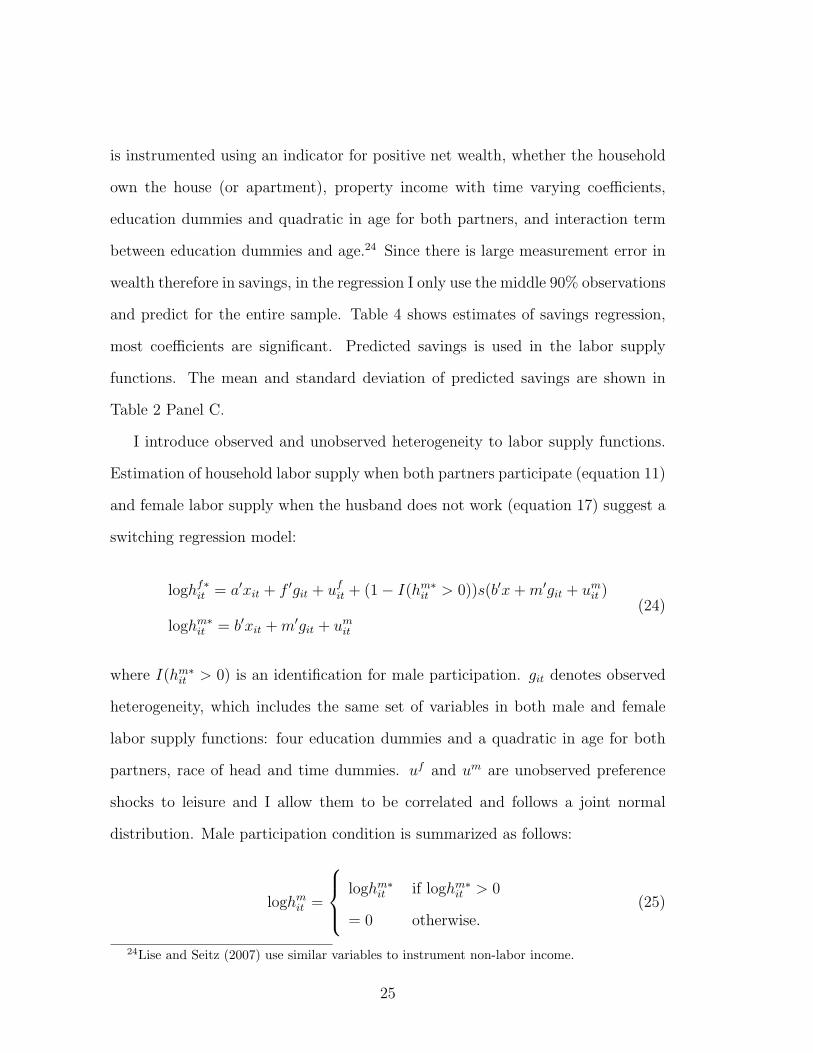
I introduce observed and unobserved heterogeneity to labor supply functions.

Estimation of household labor supply when both partners participate (equation 11)

and female labor supply when the husband does not work (equation 17) suggest a

switching regression model:

loghf∗it = a′xit + f ′git + ufit + (1− I(hm∗it > 0))s(b′x+m′git + umit )

loghm∗it = b′xit +m′git + umit

(24)

where I(hm∗it > 0) is an identification for male participation. git denotes observed

heterogeneity, which includes the same set of variables in both male and female

labor supply functions: four education dummies and a quadratic in age for both

partners, race of head and time dummies. uf and um are unobserved preference

shocks to leisure and I allow them to be correlated and follows a joint normal

distribution. Male participation condition is summarized as follows:

loghmit =

loghm∗it if loghm∗it > 0

= 0 otherwise.(25)

24Lise and Seitz (2007) use similar variables to instrument non-labor income.

25

Equation (24) and (25) are estimated using Full Information Maximum Likelihood

(FIML). Likelihood function is given in Appendix B.

4.3.1 Estimates of Reduced Form Supply Functions

Table 5 presents FIML estimates of reduced form female and male labor supply

functions. One’s wage shocks, either permanent or transitory, have significant

negative effect on spousal labor supply, while permanent shocks have a larger

impact than transitory shocks. When the husband gets a one percent negative

permanent shock in his hourly wage, the wife increases her labor supply by 0.16

percent.25 When his transitory wage drops one percent, on the other hand, the

wife’s labor supply increases by 0.04 percent. Similar effect can be found in male

labor supply functions: a one percent drop in the wife’s permanent wage shock

increases male labor supply by 0.18 percent, while same drop in transitory shock

increases male labor supply by 0.13 percent. This suggests that household members

insure each other by increasing labor supply in response to spousal adverse shocks,

and such insurance effect is stronger for more persistent shocks. The estimate of

ρ is −0.058, which suggests couples’ unobserved preference shocks to leisure are

negatively correlated.

Unlike wage shocks, the predicted wage wjit, has positive effect on spousal labor

supply. One percent increase in wmit tends to increase female labor supply by 0.21

percent, while same increase in wfit tends to increase male labor supply by 0.45

percent.

25Notice both wage rate and labor supply are logarithm, the estimates represent elasticity.

26

4.3.2 Recover Parameters on Mashallian Labor Supply and Sharing

Rules

To find out whether empirical results are consistent with collective hypothesis,

I test the restrictions implied by collective model and unitary model. Testing

restrictions for collective model is stated in equation (11) and (12). Wald statistic

from a joint test is 6.29 with a p-value of 0.279, which suggests that I cannot

reject collective hypothesis at 1%, 5% or even 10% level. Testing restrictions for

unitary model, equation (19) and (20), has a statistic of 11.93 and p-value of

0.0026, which means the unitary model can be significantly rejected at 1 percent

level. Collective model can not be rejected while unitary model can be rejected.

This provide support for the collective hypothesis.

From estimation of reduced form labor supply functions, I recover Mashallian

labor supply of equation (5) up to an additive constant. Table 6 presents female and

male Mashallian labor supply estimates. The income effect is precisely estimated

and is negative for male labor supply, which suggests male leisure is a normal good.

Female income effect is also negative but is not precisely estimated. Both male and

female wage effect are significantly positive. The implied wage elasticity is 0.605 for

female and 1.604 for male at the sample mean. Both male and female Mashallian

labor supplies satisfy Slusky condition of individual utility maximization, which is

a requirement from theory.

Table 7 presents estimates of the two sharing rules, the first one is associated

with when both partners are working, the second one is associated with only the

wife is working but the husband is not.26 Standard errors are computed using

delta method. Some of the estimates are not precisely determined. Looking at

26On male nonparticipation set, transitory wage shock is missing, thus the sharing rule φNPit

does not depend on male transitory shock.

27

equation (10) we may find that each parameter in the sharing rule rely on five

parameters from the reduced form labor supply, and every sharing rule parameter

depends on the estimates of ∆ = a1b8−b1a8. Furthermore, even if each coefficients

are estimated significantly, ∆ still may show up insignificant, especially when a1b8

and b1a8 have the same sign (Bloemen 2004). Thus it is particularly important to

obtain good estimates of nonlabor income to get a1 and b1 and the first distribution

factor to get a8 and b8.27

When both partners are working, a household makes more transfer to the agent

with adverse shocks, and makes larger transfer to the agent with shocks that are

permanent. A $1 negative permanent shock to female hourly log wage, which is

equivalent to a $10 drop in hourly wage or $7,200 drop in her earnings over four

months full-time work, increases her share of non-labor income over four months

by $90.9. Meanwhile, same unit negative transitory shock increases her share of

non-labor income by $63.7. The effects are significant at 1 percent level. When

the husband gets adverse wage shocks, he also gets more pooled income from this

intra-household allocation, but the effects are not significant, with p-value of 0.12

and 0.18 respectively. Estimation of the sharing rule on working couples provides

some evidence on insurance against permanent and transitory shocks by making

intra-household allocation and labor supply.

The increase of female group specific wage wfit or the decrease of male group

specific wage wmit , on the other hand, increases the proportion of household pooled

income allocated to the wife. This result is also found in collective labor supply

estimation in Blundell et al. (2007). Their interpretation is that higher wage

increases one’s bargaining power within household, thus he or she could get more

27Table 7 use local sex ratio as the first distribution factor, I also tried using divorce law indexas the first distribution factor, the results do not change much.

28

resources from intra-household allocation. This effect is precisely determined for

female but not well determined for male.

The sharing rule for a working wife with a nonworking husband is quite different

from the rule for working couples, due to the large value of the estimate of q

in equation (16). When the wife gets an adverse shock, no matter permanent

or transitory, her share of household non-labor income no longer increases. The

intuition behind this result is that now the husband is not able to adjust his

labor supply, therefore even if the wife has adverse shock, the husband could not

provide insurance through labor supply. The estimates of this sharing rule also

suggests that I do not find added worker effect in the data. Added worker effect

suggests when the husband gets unemployed, the wife works more to compensated

for his income loss, which is contrary to what the sharing rule shows. However,

the estimates of this sharing rule are not significant even at 10% level, partly due

to the insignificant estimates of q. The coefficient estimate of non-labor income

has a value of 1.31, which is outside the reasonable range between 0 and 1.28

The distribution factors does not have expected sign on the sharing rule. In-

crease in local sex ratio (the relative scarcity of women) and the change of divorce

law that in favor of women should increase female share of non-labor income, but

I find either no significant effect or opposite effect. I also tried alternative mea-

surement of sex ratio, such as divided into four racial groups instead of three,

or measure the number of men over men plus women within 5-year-old group or

10-year-old group. Results do not change qualitatively. This unexpected sign for

distribution factors is also found in Hourriez (2005). They argue that such effect

28I also perform test to see whether permanent shocks and transitory shocks have the sameimpact on intra-household allocation or labor supply, and whether there is a symmetric responsefrom the husband and the wife. However, since estimates of sharing rule only significant forfemale permanent shocks and transitory shocks when both partners are working, I only test thiseffect and the null hypothesis of equal effect can not be rejected.

29

may be a consequence of home production. When the wife’s options outside mar-

riage become better off, she may want to negotiate both the share of non-labor

income and a reduction in her housework. This explanation is also compatible with

results in Table 7. Increase of scarcity of women decrease male share of non-labor

income when the husband participates in the labor market, as couples may bargain

over housework. The higher bargaining power the husband has, he can negotiate

to get less housework, therefore might increases his labor supply. Such effect of

sex ratio on sharing rule is no longer significant when the husband does not par-

ticipate. This might due to the fact that husband devotes zero hours on market

work therefore his time on home production is almost fixed, thus the wife does not

need to negotiate over home production, then only negotiate on intra-household

allocation. This is why I find a positive effect of distribution factors on sharing

rule when the husband does not participate in labor market.

4.4 Insurance for Liquidity Constrained Households

When households have limited access to borrowing and could not adjust savings

to insure against income shocks, household members may be more likely to adjust

labor supply to smooth consumption. Added worker effect literature have found

mixed evidence on the relationship between the smoothing role of spousal labor

supply and liquidity constraints. Garcia-Escribano (2004) uses data from PSID

and finds that wives’ labor response to transitory shocks in husbands’ earnings is

larger for households with limited access to credit. Dynarski and Gruber (1997)

uses data from the PSID and Consumer Expenditure Survey (CEX) and find that

the sample drawn from the PSID response of spousal labor supply is insignificant,

while in the CEX sample her labor response is not significant for high school

30

dropouts, but significant and even larger effect for higher educated groups, which

seems to contradict the liquidity constraints story. This section explores whether

and how couples adjust labor supply to insure against wage shocks when they face

liquidity constraints.

I define liquidity constraints as households whose net wealth in the third wave

is less than the 50th percentile.29 Table 8 displays results of reduced form labor

supply and Table 9 displays results for the sharing rules. Reduced form estimates

show that one’s permanent shocks have significant effect on spousal labor supply

at 1 percent level, while transitory shocks do not even at 10 percent level. This

is different from estimation over the whole sample, where both permanent shocks

and transitory shocks have significant effect on spousal labor supply at 1 percent

level. In Table 9, parameters on sharing rules are poorly estimated thus I could

not compare it with previous results using entire sample. Alternative measures of

liquidity constraints are also tried as robustness checks: household income in the

first wave is less than the 50th percentile; household head’s education with high

school degree or below, or households with net wealth less than the 50th percentile

and do not own house or apartment. Results do not change qualitatively. These

empirical findings are not exactly consistent with liquidity constraints theory, but

many factors could explain these results: liquidity constrained households are more

likely to have lower income, lower education, which restrict household members’

ability of finding jobs or adjust labor supply in short period. This also explains

why couples with limited liquidity only respond to permanent shock but not to

transitory shock.

29I choose the third wave because this is the first wave that net wealth is observed instead ofinterpolated.

31

4.5 Do Couples Insure against Shocks or Volatility?

Previous sections examine whether and how married couples insure against each

other’s adverse wage shocks. Another question of interest is whether they also

insure against individual wage volatility, which can be measured as the variance

of wage shocks for each individual.

Table 10 displays estimates of sharing rules including individual variance of

wage shocks. Permanent shocks and transitory shocks still affect the sharing rule

in the same direction as in Table 7. The point estimates show that higher indi-

vidual wage volatility causes a lower proportion of non-labor income, both for the

husband and the wife. One explanation is that agent with higher income uncer-

tainty might have lower bargaining power in the household. On the contrary, when

the husband is not working, the higher the variation of his shocks in other periods,

the more resources he will get from intra-household allocation. However, due to

the insignificancy of the effect of female wage volatility on male labor supply, the

sharing rule parameters are not precisely estimated. Recall that the sample only

covers three years data, and the variance of wage shocks over such short period

might not provide a sufficient statistic for actual wage volatility.30 In the mean-

time, as existing studies in marital sorting literature have pointed out, people tend

to search for spouse who has negative income covariance with themselves, or look

for someone who has stable job and stable income. Income volatility might already

be insured via marriage decision, and after getting married there is little we can see

about insurance against this uncertainty. Overall, Table 10 shows little evidence

of household insurance against wage volatility.

30Note that in the section of stylized facts, income volatility is estimated using entire sample,here wage volatility is computed at individual level. These are two different notations and that’swhy I call the latter one “individual wage volatility”.

32

4.6 Comparison with Baseline Model that Does not In-

cluding Shocks

This paper introduces permanent shocks and transitory shocks into the sharing

rule of collective model. In this section I estimate the baseline model in existing

collective literature, which do not distinguish between wage with its stochastic

shocks. Table 11 displays sharing rule estimates which treat wage as single com-

ponent, given everything else same as my main sample and method. The effect of

female wage on sharing rule is significant negative, Chiappori et al. (2002) inter-

pret this result as altruism. Male wage effect is not significant. Two distribution

factors now have the expected positive sign but are still not precisely estimated.

Comparing this result with the main results in Table 7, the effect of wage com-

ponent wit reverses the sign. This shows the importance of distinguish wage and

wage shocks, and distinguish between shocks that are permanent and transitory.

Table 12 displays results that only consider the case when both partners are

working, which is the sample defined in Chiappori et al. (2002). Again female

wage has negative effect on the sharing rule, male wage effect is not significant.

Compare the estimated coefficient of distribution factors in Table 11 and Table 12,

the coefficient reverses sign. This also shows incorporating nonparticipation into

the sharing rule might be important.

4.7 Robustness Check and Further Discussion

As an alternative to including male nonparticipation, I also estimate model includ-

ing continuous labor supply with female nonparticipation only. Table 13 displays

reduced form labor supply estimates and Table 14 displays sharing rule estimates.

Unfortunately all parameters in the sharing rule are poorly determined, mainly

33

due to the imprecise estimates of both distribution factors. The sign of the point

estimators for permanent and transitory shocks of each agent are still the same as

main results in Table 7, where the sample includes nonworking husbands but not

nonworking wives. This provides a robustness check of the main results.

I also estimate the main model using several alternative specifications. First

I redefine the sample to exclude households with children less than 6 years old

instead of excluding households with children less than 18 years old in the main

sample. This gives me a larger sample size but qualitative results do not change.

I use weekly hours worked instead of total hours worked in period t, and the

estimation results do not change either. I also try to estimate the model using

the sample of hourly workers only. This will get rid of the endogeneity problem

caused by imputed wage from earnings. Unfortunately, the parameters are very

poorly estimated, mainly because of very small sample size. In SIPP data the flag

for imputed wage has lots of missing values, and when restrict sample on both

partners who are hourly workers, it only gives me a pool of 886 households, while

the main sample contains 4,749 households. Overall, these specification checks

show that main results are robust to various specifications and sample cuts.

I acknowledge some limitations both from theory and empirical work in this

paper. This model assumes agents can adjust labor supply freely, while in reality

hours might be constrained for a given job, and it takes time to get another job so

that the labor supply adjustments by switching jobs are not reflected in the current

period. Therefore, empirical work might underestimate the effect of wage shocks on

labor supply. On the other hand, a huge negative shock from one partner may leads

to divorce, which drops that households out of my sample. Thus my estimation uses

the most committed families and this tends to overestimate households’ willingness

on insurance. Focusing on married couples without children and excludes sample

34

of nonworking wives may also cause selection bias. Estimation results in this paper

only have policy implications on married couples without children.

Another limitation comes from the estimation of wage shocks. This model takes

wage shocks as given, but some shocks could be endogenous to one’s own labor

supply or spousal labor supply. This limitation can be resolved if I have some

measure of exogenous wage shocks. It is also possible that wage changes because

of location change. If an individual moves from a big city to a small town and

gets a better job, the nominal wage might still drop because the living standard is

much lower in small town, but the agent does not think of it as an adverse shock

and would not response to that.

This model does not consider the interaction between social insurance program

such as unemployment benefit and intra-household insurance.31 For the conve-

nience of estimation, utility functions does not have risk aversion parameters. But

preference to risk could be a factor that influence couples’ willingness to insure.

For instance, more risk averse households may be more likely to insure each other’s

transitory shocks to smooth consumption, or if a husband and a wife have differ-

ent preference for risk, they may respond to spousal shocks differently. Above

discussions in this section suggest some important avenues for future research.

5 Conclusion

The aim of this paper has been to evaluate the link between income volatility

and household decision through the degree of household labor supply insurance

with respect to wage shocks, both permanent and transitory. I develop a life-cycle

collective model, where wage are stochastic and the intra-household allocation de-

31Cullen and Gruber (2000) show that the generous unemployment benefit has a crowd outeffect on spousal labor supply.

35

pends on both permanent and transitory wage shocks. I first estimate permanent

and transitory wage shocks for each individual, then estimate couples labor sup-

plies using SIPP 2001 panel and recover the unobserved intra-household allocation

mechanism. Estimation results provide some evidence on household insurance via

labor supply: married couples making joint labor supply decisions to insure against

both permanent and transitory wage shocks, while labor response is larger when

shocks are permanent. Such household insurance disappears when the husband

gets unemployed and could not adjust his labor supply. There is little evidence

of insurance from labor supply for liquidity constrained households, and little ev-

idence of insurance against high individual wage volatility. This paper not only

provides structural explanation of household insurance through labor supply, but

also contributes to the empirical studies using collective model by using high-

frequency data in the U.S. and incorporating nonparticipation. Estimation and

the comparison with existing collective models shows the importance of stochastic

wage components therefore the importance of developing formal dynamic collective

models with labor supply both on extensive and intensive margin.

The structural analysis of household insurance via labor supply provides an

explanation on why individual income volatility does not completely translate into

household income volatility, as stylized facts have shown. Meanwhile, lacking of

insurance opportunities leads to a greater vulnerability to income shocks. How

well household smooth income shocks also provide an important complement to

the understanding of public insurance policies and redistributive policies.

36

Appendix

A Proof of Existence of Pareto Weight

Browning, Chiappori and Lewbel (2007) prove a dual representation of the house-

hold problem. From their Proposition 1, there exists a shadow price vector and

a scalar valued sharing rule to solve the household problem in equation (2). By

Proposition 2, given the shadow price vector and the sharing rule, there exists a

Pareto weight which can be written as a function of indirect utility functions and

the sharing rule. Let vf and vm denote indirect utility functions for the wife and

the husband. By Roy’s identify:

∂vf (wfit, φfit)/∂w

fit

∂vf (wfit, φfit)/∂φ

fit

= hfit,∂vm(wmit , φ

mit )/∂w

mit

∂vm(wmit , φmit )/∂φ

mit

= hmit (26)

First, from Mashallian labor supply functions in equation (5), the differential

equations above can be integrated out to get the following indirect utilities:

vf (wfit, φfit) =

e−α2φfit

α2

+(wfit)

α1+1

α1 + 1

vm(wmit , φmit ) =

e−β2φmit

β2

+(wmit )

β1+1

β1 + 1

(27)

By Proposition 2 in Browning, Chiappori and Lewbel (2007), the above indirect

utility functions imply the following Pareto weight:

µit = −∂vm(wmit , φ

mit )/∂φit

∂vf (wfit, φfit)/∂φit

=e−β2φm

it

e−α2φfit

= e(α2+β2)φit−β2(yit−sit) (28)

37

Substituting φit with equation (6) we get:

µit = eα2+β2[(k0+(k1−1)(yit−sit)+k2wfit+k3w

mit +k4δ

fit+k5δ

mit +k6ν

fit+k7ν

mit +k8z1i+k9z2i] (29)

B Derivation of Likelihood Function

First assume preference shocks ufit and umit in labor supply functions follows a joint

normal distribution with zero mean and the following covariance matrix:

σ2f ρσfσm

ρσfσm σ2m

The log-likelihood function takes the form:

L =∑i∈P

logLi(hfit, h

mit ) +

∑i∈NP

logLi(hfit) (30)

Likelihood function when both partners are working is straightforward, following

a joint normal distribution:

Li(hfit, h

mit ) =

1

σfσmϕ(ufitσf,umitσm

, ρ) (31)

where ϕ is standard normal distribution function. The likelihood function in male

nonparticipation set NP is different. First, the covariance matrix becomes:

σ2f + 2sρσfσm + s2σ2

m ρσfσm + sσ2m

ρσfσm + sσ2m σ2

m

38

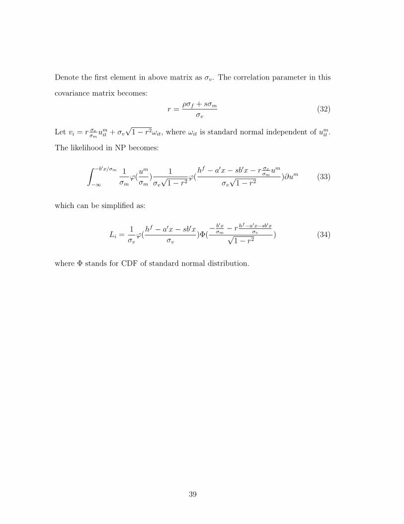
Denote the first element in above matrix as σv. The correlation parameter in this

covariance matrix becomes:

r =ρσf + sσm

σv(32)

Let vi = r σv

σmumit + σv

√1− r2ωit, where ωit is standard normal independent of umit .

The likelihood in NP becomes:

∫ −b′x/σm

−∞

1

σmϕ(um

σm)

1

σv√

1− r2ϕ(hf − a′x− sb′x− r σv

σmum

σv√

1− r2)∂um (33)

which can be simplified as:

Li =1

σvϕ(hf − a′x− sb′x

σv)Φ(− b′xσm− r hf−a′x−sb′x

σv√1− r2

) (34)

where Φ stands for CDF of standard normal distribution.

39

References

Attanasio, O. and N. Pavoni (2007). Risk Sharing in Private Information Models

with Asset Accumulation: Explaining the Excess Smoothness of Consumption.

Number 12944 in NBER Working Paper Series.

Bloemen, H. G. (2004). An Empirical Model of Collective Household Labour Sup-

ply with Nonparticipation. Free University Amsterdam Serie Research Memo-

randa No. 0002.

Blundell, R., P.-A. Chiappori, T. Magnac, and C. Meghir (2007). Collective La-

bor Supply: Heterogeneity and Nonparticipation. Review of Economic Stud-

ies 74 (2), 417–45.

Blundell, R., L. Pistaferri, and I. Preston (2008). Consumption Inequality and

Partial Insurance. American Economic Review (forthcoming).

Blundell, R. and I. Walker (1986). A Life-cycle Consistent Empirical Model of Fam-

ily Labour Supply using Cross-Secion Data. Review of Economic Studies 53 (4),

539–58.

Browning, M., P.-A. Chiappori, and A. Lewbel (2007). Estimating Consumption

Economies of Scale, Adult Equivalence Scales, and Household Bargaining Power.

Number 588 in Boston College Working Paper Series.

Chiappori, P.-A. (1988). Rational Household Labor Supply. Econometrica 56 (1),

63–89.

Chiappori, P.-A. (1992). Collective Labor Supply and Welfare. Journal of Political

Economy 100, 437–67.

Chiappori, P.-A., B. Fortin, and G. Lacroix (2002). Marriage Market, Divorce

Legislation and Household Labor Supply. Journal of Political Economy 110 (1),

37–72.

Cullen, J. B. and J. Gruber (2000). Does Unemployment Insurance Crowd out

Spousal Labor Supply. Journal of Labor Economics 18 (3), 546–72.

Donni, O. (2003). Collective Household Labor Supply: Nonparticipation and In-

come Taxation. Journal of Public Economics 87, 1179–98.

40

Dynarski, S. and J. Gruber (1997). Can Families Smooth Variable Earnings?

Brookings Papers on Economic Activity 1997 (1), 229–303.

Garcia-Escribano, M. (2004). Does Spousal Labor Smooth Fluctuations in Hus-

bands’ Earnings? The Role of Liquidity Constraints. IMF Working Paper

WP/04/20.

Gottschalk, P. (2005). Downward Nominal Wage Flexibility–Real or Measurement

Error? Review of Economics and Statistics .

Gottschalk, P. and R. Moffitt (1994). The Growth of Earnings Instability in the

U.S. Labor Market. Brookings Papers on Economic Activity 1994 (2), 217–72.

Hall, R. and F. Mishkin (1982). The Sensitivity of Consumption to Transitory

Income: Estimates from Panel Data of Households. Econometrica 50 (2), 261–

81.

Hourriez, J.-M. (2005). Estimation of a Collective Model of Labor Supply with

Female Nonparticipation. CREST-INSEE mimeo.

Lise, J. and S. Seitz (2007). Consumption Inequality and Intra-Household Alloca-

tions. Queen’s Economics Department Working Paper No. 1019.

Mazzocco, M. (2004). Saving, Risk Sharing, and Preferences for Risk. American

Economic Review 94 (4), 1169–82.

Mazzocco, M. (2005). Individual Rather Than Household Euler Equations: Iden-

tification and Estimation of Individual Preferences Using Household Data. Uni-

versity of Wisconsin-Madison.

Mazzocco, M. (2007). Household Intertemporal Behaviour: A Collective Char-

acterization and a Test of Commitment. Review of Economic Studies 74 (3),

857–95.

Mazzocco, M. and S. Yamaguchi (2006). Labor Supply, Wealth Dynamics, and

Marriage Decisions. California Center for Population Research Paper CCPR-

065-06.

Moffitt, R. and P. Gottschalk (2008). Trends in the Transitory Variance of Male

Earnings in the U.S., 1970-2004. Mimeo.

41

Vermeulen, F. (2005). A Collective Model for Female Labor Supply with Non-

participation and Taxation. Journal of Population Economics (19), 99–118.

42

0

0.2

0.4

0.6

0.8

1982

1984

1986

1988

1990

1992

1994

1996

1998

2000

2002

Log Household Earnings

Log Male Earnings

Log Female Earnings

Figure 1: Transitory Variances of Log Household Earnings, Log Male Earningsand Log Female Earnings in the U.S., Married Households from PSID 1979-2002

43

Table 1: Comparison of Transitory Variances for Married and Single Agents

Transitory VariancesLog Household Earnings Log Household Income

Singles(random match) 0.141 0.135Married Couples 0.092 0.085

Log Wage rate Log Earnings Log HoursSingle Males 0.044 0.174 0.036Single Females 0.047 0.180 0.040Married Males 0.058 0.169 0.041Married Females 0.074 0.224 0.065

Note: transitory variances are calculated as: var(εit) = 1N

N∑i

1(Ti−1)

Ti∑i

(yit−yi)2

44

Table 2: Descriptive Statistics

StandardMean Deviation Minimum Maximum

A. WomenHours of work 411.1 344.9 0 2,358Hourly wage 12.4 13.66 0.0001 705.7Age 38.8 9.37 20 59Schooling 18.5 5.91 1 26White 0.87 0.33 0 1

B. MenHours of work 613.3 350.2 0 2,592Hourly wage 18.3 15.05 0.003 401.8Age 40.9 9.36 20 59Schooling 18.7 5.95 1 26White 0.88 0.33 0 1

C. Household CharacteristicsNonlabor income 1,154.4 3,004.5 0 90,967Savings (predicted) 6,227.7 5810.2 -46,788 116,815Own living quarters 0.79 0.4 0 1

D. Marriage MarketSex ratio 0.498 0.021 0.227 0.813Divorce index 2.410323 0.718819 1 4

E. Participation StatusWife works Wife not work

Husband works 54.5% 25.7%Husband not work 10.9% 8.6%

Table 3: Summary of Log Wage Decomposition

StandardMean Deviation Minimum Maximum

Female Group Specific Wage (wfit) 2.17 0.368 0.82 2.80Male Group Specific Wage (wmit ) 2.67 0.297 1.73 3.23

Female Permanent Shock (δfit) -0.0002 0.815 -10.57 3.14Male Permanent Shock (δmit ) -0.0008 0.660 -8.60 3.03

Female Transitory Shock (νfit) 0.0002 0.253 -8.26 7.27Male Transitory Shock (νmit ) 0.0001 0.231 -6.09 3.59

45

Table 4: Estimates from Savings Equation

Coefficient Standard ErrorPositive net wealth -10,960.2** 600.3Own house 3,8968*** 426.5Male age 750.8*** 241.1Female age 665.6*** 224.3Male age square -8.61*** 2.76Female age square -6.09*** 2.71Asset income (t=1) -0.108 0.298Asset income (t=2) -0.890** 0.370Asset income (t=3) -0.739** 0.380Asset income (t=4) -0.511 0.470Asset income (t=5) -0.818 0.558Asset income (t=6) 1.584*** 0.470Asset income (t=7) 1.702*** 0.424Asset income (t=8) 2.701*** 0.475

Note: (1)***significant at 1%; **significant at 5%; *significant at 10%. (2)Othervariables: four education dummies, education dummies interact with age for bothpartners.

46

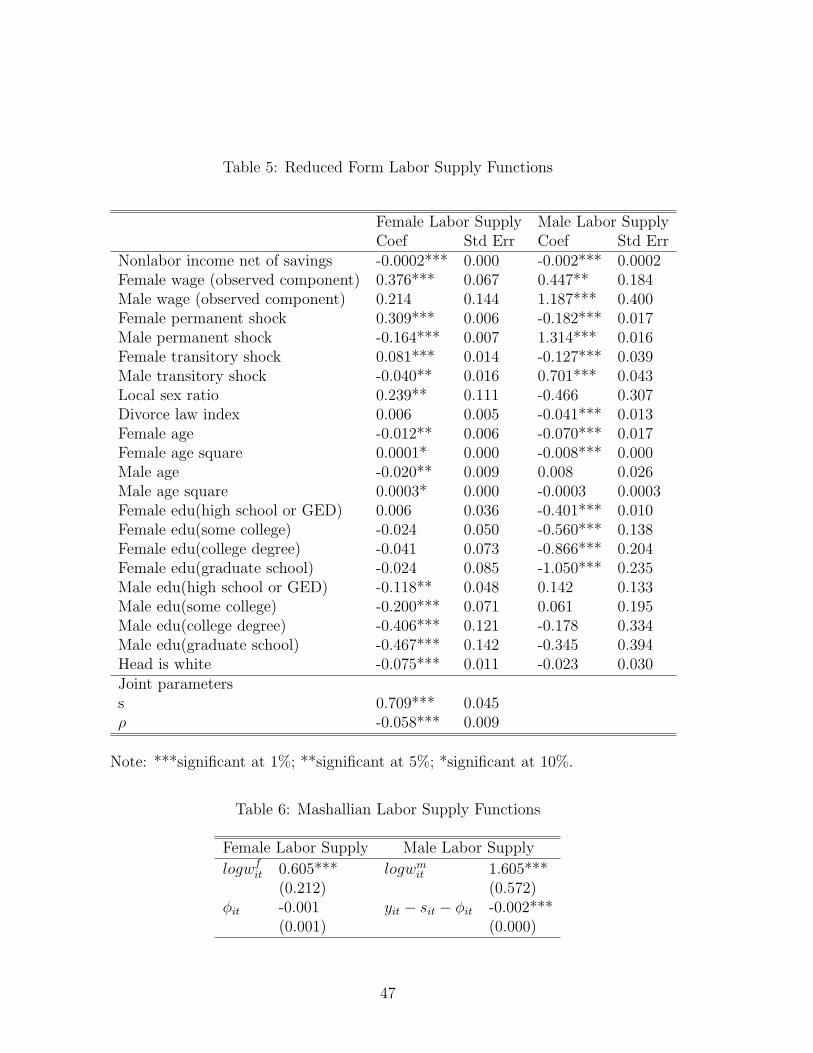
Table 5: Reduced Form Labor Supply Functions

Female Labor Supply Male Labor SupplyCoef Std Err Coef Std Err

Nonlabor income net of savings -0.0002*** 0.000 -0.002*** 0.0002Female wage (observed component) 0.376*** 0.067 0.447** 0.184Male wage (observed component) 0.214 0.144 1.187*** 0.400Female permanent shock 0.309*** 0.006 -0.182*** 0.017Male permanent shock -0.164*** 0.007 1.314*** 0.016Female transitory shock 0.081*** 0.014 -0.127*** 0.039Male transitory shock -0.040** 0.016 0.701*** 0.043Local sex ratio 0.239** 0.111 -0.466 0.307Divorce law index 0.006 0.005 -0.041*** 0.013Female age -0.012** 0.006 -0.070*** 0.017Female age square 0.0001* 0.000 -0.008*** 0.000Male age -0.020** 0.009 0.008 0.026Male age square 0.0003* 0.000 -0.0003 0.0003Female edu(high school or GED) 0.006 0.036 -0.401*** 0.010Female edu(some college) -0.024 0.050 -0.560*** 0.138Female edu(college degree) -0.041 0.073 -0.866*** 0.204Female edu(graduate school) -0.024 0.085 -1.050*** 0.235Male edu(high school or GED) -0.118** 0.048 0.142 0.133Male edu(some college) -0.200*** 0.071 0.061 0.195Male edu(college degree) -0.406*** 0.121 -0.178 0.334Male edu(graduate school) -0.467*** 0.142 -0.345 0.394Head is white -0.075*** 0.011 -0.023 0.030Joint parameterss 0.709*** 0.045ρ -0.058*** 0.009

Note: ***significant at 1%; **significant at 5%; *significant at 10%.

Table 6: Mashallian Labor Supply Functions

Female Labor Supply Male Labor Supply

logwfit 0.605*** logwmit 1.605***(0.212) (0.572)

φit -0.001 yit − sit − φit -0.002***(0.001) (0.000)

47

Table 7: Estimates of the Sharing Rules

Both partners work Wife works, husband notCoef Std Err Coef Std Err

yit − sit 0.19 0.13 1.31 0.83

wfit 223.6** 101.1 -85.7 231.9wmit -209.1 194.0 -1,030.5 725.9

δfit -90.9*** 19.02 34.8 93.35δmit 160.4 103.1 -749.2 484.0

νfit -63.8*** 22.67 24.4 65.87νmit 39.3 29.54 - -Local sex ratio -233.2* 129.9 89.3 288.7Divorce law index -6.12 5.97 22.5 18.1q - - -692.1 446.3

Table 8: Reduced Form Labor Supply Function Estimation for Liquidity Con-strained Households

Female Labor Supply Male Labor SupplyCoef Std Err Coef Std Err

Nonlabor income net of savings -0.0002 0.0002 -0.004*** 0.0005Female wage (observed component) 0.979*** 0.214 0.352 0.564Male wage (observed component) 0.457 0.432 3.597*** 1.134Female permanent shock 0.309*** 0.017 -0.292*** 0.044Male permanent shock -0.097*** 0.024 1.356*** 0.045Female transitory shock 0.188*** 0.042 -0.133 0.111Male transitory shock -0.029 0.042 0.968*** 0.109Local sex ratio -0.424 0.268 -0.305 0.709Divorce law index -0.005 0.014 -0.094*** 0.365

Note: ***significant at 1%; **significant at 5%; *significant at 10%

48

Table 9: Estimates of the Sharing Rule for Liquidity Constrained Households

Both partners work Wife works, husband notCoef Std Err Coef Std Err

yit − sit -0.633 3.072 -0.693 3.300

wfit 1627.2 5,418.58 1,686.42 5,683.19wmit 1523.4 7,190.29 2,128.81 10020

δfit -1349.9 3,929.30 -1,399.03 4131.93δmit -322.60 1,493.23 -94.42 655.92

νfit -616.51 1,856.5 638.92- 1,952.42νmit -98.30 474.72 - -Local sex ratio -1,412.57 6,340.39 -1,463.95 6,766.21Divorce law index -18.14 94.85 -34.02 167.54q - - 168.32 873.60

Table 10: Estimates of the Sharing Rules including Individual Income Volatility

Both partner works Husband works, wife notCoef Std Err Coef Std Err

yit − sit 0.140** 0.056 0.929*** 0.229

wfit 240.34** 102.95 19.73 64.78wmit -120.86 104.71 -580.88** 265.45

δfit -100.60*** 14.726 -8.25 7226δmit 115.10*** 30.83 -530.78*** 146.14

νfit -58.79*** 21.74 -4.82 15.92νmit 25.56** 12.52 - -σνf -41.67*** 10.48 -3.419 10.33σνm 29.60*** 11.40 -86.52*** 29.89local sex ratio -151.87* 85.73 31.96 165.13divorce law index -3.97 3.41 16.13* 8.344q - - -478.20*** 130.32

49

Table 11: Baseline Sharing Rules that Does not Distinguish Wage and Shocks

Both partner works Husband works, wife notCoef Std Err Coef Std Err

yit − sit -0.007 0.27 -0.012 0.031

wfit -57.13*** 10.69 -28.8*** 9.13wmit -29.20 97.82 -47.77 98.37Local sex ratio 52.73 171.3 86.27 169.8Divorce law index 0.906 3.12 1.48 3.28q - - 107.9*** 12.26

Table 12: Baseline Sharing Rules that Does not Distinguish Wage and Shocks andExcludes Nonparticipation

Coef Std erryit − sit 0.091 0.206

wfit -18.11*** 4.826wmit 9.44 21.21Local sex ratio -17.52 38.14Divorce law index -0.54 1.26

Table 13: Reduced Form Labor Supply Function Estimation with Female Nonpar-ticipation

Female Labor Supply Male Labor SupplyCoef Std Err Coef Std Err

Nonlabor income net of savings -0.0015*** 0.0002 -0.0002*** 0.000Female wage (observed component) 2.863*** 0.235 -0.005 0.042Male wage (observed component) 0.245 0.516 0.129 0.092Female permanent shock 1.995*** 0.017 -0.090*** 0.004Male permanent shock -0.488*** 0.025 0.123*** 0.004Female transitory shock 1.006*** 0.050 -0.033*** 0.009Male transitory shock -0.226*** 0.057 0.023*** 0.010Local sex ratio -0.021 0.016 -0.011*** 0.070Divorce law index 0.418 0.392 -0.016 0.003

Note: ***significant at 1%; **significant at 5%; *significant at 10%.

50

Table 14: Estimates of the Sharing Rule with Female Nonparticipation

Both partners work Husband works, wife notCoef Std Err Coef Std Err

yit − sit 0.249 0.796 -1.312 2465

wfit -21.33 175.25 2,890.5 3,119.2wmit -39.71 151.95 209.15 590.41

δfit -374.61 402.62 1,654.5 1,777.5δmit 79.12 252.68 -416.7 781.14

νfit -138.71 153.44 884.5 952.2νmit 36.72 117.62 - -Local sex ratio 3.432 11.32 -18.08 36.77Divorce law index -67.86 220.03 357.4 776.5q - - 1016.92 1092.54

Note: Asymptotic standard errors are computed using delta method.

51