The Effect of News Shocks and Monetary Policy∗

Luca Gambetti†

Universitat Autonomade Barcelona

Dimitris Korobilis‡

University of Essex

John D. Tsoukalas§

University of GlasgowFrancesco Zanetti¶

University of Oxford

September 2017

Abstract

A VAR model estimated on U.S. data before and after 1980 documents systematicdifferences in the response of short- and long-term interest rates, corporate bondspreads and durable spending to news TFP shocks. Interest rates across thematurity spectrum broadly increase in the pre-1980s and broadly decline in thepost-1980s. Corporate bond spreads decline significantly, and durable spendingrises significantly in the post-1980 period while the opposite short-run responseis observed in the pre-1980 period. Measuring expectations of future monetarypolicy rates conditional on a news shock suggests that the Federal Reserve hasadopted a restrictive stance before the 1980s with the goal of retaining controlover inflation while adopting a neutral/accommodative stance in the post-1980period.

Keywords: News shocks, Business cycles, VAR models, DSGE models

JEL Classification: E20, E32, E43, E52

∗We thank Paul Beaudry, Jean-Guillaume Sahuc and seminar participants at the Banque de Franceand the University of Oxford for extremely valuable comments. Some of this work was completed whileJohn Tsoukalas and Francesco Zanetti were visiting scholars at the Banque de France; they would liketo thank the Foundation Banque de France for its support. Financial support from the LeverhulmeTrust Research Project Grant RPG-2014-255 is gratefully acknowledged.†Departament d’Economia i d’Historia Economica, 08193 Bellaterra, Spain.‡Essex Business School, Wivenhoe Park, Colchester, CO4 3SQ, U.K.§Adam Smith Business School, Gilbert Scott Building, Glasgow, G12 8QQ, U.K.¶Department of Economics, Manor Road, Oxford, OX1 3UQ, U.K.

1 Introduction

The effect of anticipated changes in future total factor productivity (TFP)—the so-called

news shocks—on current macroeconomic outcomes has spurred considerable research

interest over the past few years. Several studies find that news shocks exert strong

influence on expectations about future economic conditions and thus lead to sizable

changes in current economic activity.1 This paper establishes new empirical facts about

changes in the transmission and propagation of news shocks over time and finds that

they are tightly linked to systematic changes in the conduct of monetary policy.

To isolate differences in the effect of news shocks across time, we estimate a vector

autoregression (VAR) model on two subsamples of U.S. data, before and after 1980.

We apply the identification approach in Forni et al. (2014), whereby a TFP news shock

best anticipates TFP in the long run without changing current TFP.2 We find that

responses of nominal short- and long-term interest rates to a news TFP shock exhibit

a sign reversal between subperiods. A positive news TFP shock is associated with

a delayed rise in short- and long-term nominal interest rates before the 1980s. By

contrast, the same shock is associated with a fall in these same rates after the 1980s.

We investigate whether these sharp sign reversals in the response of nominal rates are

related to systematic differences in the conduct of monetary policy using the Expectation

Hypothesis as our organizing framework. The Expectation Hypothesis postulates that

long-term interest rates are approximated by an expectation component derived from the

weighted average of current and future short-term interest rates plus an error component

that encapsulates risk premia. The expectation component provides a powerful reading

on the conduct of monetary policy and expectations about the full range of future

policy rates. We find that the sign reversals are echoed by similar shifts in the response

1See Beaudry and Portier (2014) and references therein for a comprehensive review of the literature.2In section 2, we discuss the relationship of our identification method with alternative approaches.

1

of the expectations component in the term structure of policy yields inferred from the

Expectation Hypothesis. The VAR model shows that the expectations component of

long-term rates rises persistently in response to the anticipated increase in TFP in the

pre-1980 period and declines persistently in the post-1980 period. These findings are

robust to alternative maturities of bond yields. Important for the analysis, the residual

component of the long-term interest rates remains statistically unchanged between

subperiods, suggesting that risk premia play no role for the systematic differences in

the response of the term structure of policy yields to the news shock.

These findings consistently point to substantial changes in the systematic response

of monetary policy to anticipated changes in TFP before and after the 1980s. We find

that systematic changes in the response of policy yields, as identified by the expectations

hypothesis, are mirrored by a similar reversal in the response of real interest rates, as

well as real and financial variables to news shocks between subperiods. Real interest

rates broadly maintain the sign reversal of nominal yields; namely, they rise in the

first subperiod and fall in the second subperiod. Current economic activity, hours

worked, investment and consumer durable spending decline on impact and closely track

movements in observed TFP in the pre-1980 period whereas they sharply increase on

impact and anticipate the future rise in TFP several years ahead in the post-1980 period.

These findings are consistent with the logic of the standard Euler equation, where the

entire path of real interest rates is inversely related to spending decisions, especially

for investment and durables spending. Corporate bond spreads, which proxy financial

conditions following an emerging literature, rise somewhat in the first subperiod and

decline in the second subperiod, consistent with the effect of the news shock on real

activity.3

3See Gilchrist and Zakrajsek (2012) for a treatment of financial conditions and relation with corporatebond spreads, Gortz et al. (2016), and Gortz and Tsoukalas (2017) for a discussion of the role of financialmarkets for the propagation of news shocks.

2

What is the explanation for these systematic differences in the response of policy

rates and the consequent changes in the propagation of news shocks across real and

financial variables? A wide range of influential research shows that anchoring inflation

expectations helps the central bank stabilize current inflation without requiring sharp

adjustments in the policy rate.4 To the extent that large and persistent movements

in inflation cannot occur without substantial changes in monetary policy, we can glean

information about variations in the conduct of monetary policy from the differences

in the responses of inflation and inflation expectations to anticipated changes in TFP.

The reaction of inflation expectations to the TFP news shock is significantly different

between subsamples even though the TFP news shock produces a similar impact decline

in actual inflation in both subsamples. In the first subsample, inflation expectations

increase despite a decline in actual inflation. The rise in inflation expectations coincides

with a delayed increase in economic activity generated by the news shock. By contrast,

in the second subsample, the decline in expected inflation resembles the fall in actual

inflation, despite an immediate and strong increase in economic activity. Evidently, the

increase in real activity triggered by the TFP news shock feeds into higher inflation

expectations in the first subperiod but not the second.

The stark change in the response of policy yields is tightly related to the variation in

the remit of monetary policy between subperiods. Policy rates in the pre-1980s closely

track economic activity as a result of the “lean-against-the-wind” stance of chairman

William McChensey Martin who presided over most of this period (1951-1970). During

this time, the Fed was concerned that expansionary movements in economic activity may

generate a sharp rise in inflation given the limited influence over inflation expectations.

By contrast, in the post-1980s, the Fed received a dual mandate to achieve maximum

employment, stable prices, and moderate long-term interest rates, becoming legally

4See Gertler et al. (1999), Svensson (2010) and references therein.

3

liable to maintain stable inflation.5 Under the chairmanships of Volcker, Greenspan

and Bernanke (1979-2014), the Fed effectively anchors inflation expectations, therefore

remaining unconcerned that good news about productivity may generate inflationary

pressures—even though they stimulate economic activity on impact. Our results are in

line with this intuition: the news TFP shock is associated with a persistent and mild fall

in inflation expectations. The response of the Fed, in contrast to the first subperiod, is

not to restrict the immediate rise in economic activity in the aftermath of the news shock

by raising the policy rate. Our findings are consistent with these systematic changes in

the conduct of monetary policy over time. Thus, post-1980s evidence suggests that the

Fed allowed the nominal interest rate to decline in a quest to curb the fall in actual

inflation since it was able to credibly and effectively manage inflation expectations.6

Our analysis relates to several studies focused on the effect of news shocks. Beaudry

and Portier (2004), Karnizova (2010), Fujiwara et al. (2011), Milani (2011), Schmitt-

Grohe and Uribe (2012), Ben Zeev and Khan (2015), Barsky and Sims (2011), Kurmann

and Otrok (2013) and Theodoridis and Zanetti (2016) show that anticipated movements

in future TFP have an important effect on current macroeconomic fluctuations. Our

study is the first to detect temporal variation in the effect of TFP news shocks and

establish that these differences are related to changes in the conduct of monetary policy

over time. In this respect, our analysis also contributes to the large body of research

on the changes of the effect of exogenous shocks on macroeconomic outcomes. Benati

(2004) and Bianchi et al. (2009) detect important time variation in economic performance

5See the Federal Reserve Act (ch. 6, 38 Stat. 251, enacted December 23, 1913, 12 U.S.C. ch.3). In 1977, Congress amended the Federal Reserve Act, directing the Board of Governors of theFederal Reserve System and the Federal Open Market Committee to “...maintain long run growth ofthe monetary and credit aggregates commensurate with the economy’s long run potential to increaseproduction, so as to promote effectively the goals of maximum employment, stable prices and moderatelong-term interest rates.” See Goodfriend and King (2005) for an economic account of the new monetarypolicy framework.

6An influential study by Gertler et al. (1999) shows that monetary policy can effectively influencethe economy by managing inflation expectations in addition to using changes in the policy rate.

4

related to changes in the monetary policy framework across time. Mumtaz and Surico

(2012) show global changes in the persistence and level of inflation since the 1980s

that can be explained by changes in the conduct of monetary policy and the onset of

globalization. Gambetti and Gali (2009) show that important co-movements among

output, hours and productivity significantly changed over the postwar period. Liu

et al. (2017) find important variation in the effect of monetary policy shocks during

the economy transit between different economic regimes. Finally, our results also relate

to the large literature on the effect of monetary policy for macroeconomic fluctuations.

Influential studies by Gertler et al. (1999), Ireland (2000, 2003, 2007), Boivin and

Giannoni (2006) and Castelnuovo (2012) show that the effect of exogenous shocks on the

economy depends on the stance of monetary policy. Our analysis provides novel empirical

evidence on the critical role of monetary policy for the propagation of anticipated changes

in TFP on the economy, which is consistent with changes in the conduct of U.S. monetary

policy over the postwar period.

The remainder of the paper is organized as follows. Section 2 presents data and lays

out the VAR model and the identification strategy. Section 3 discusses new facts on the

propagation of news shocks over time as well as investigates the sources of systematic

differences in the response of interest rates and macroeconomic indicators. Section 4

presents our conclusion.

2 Data and the VAR model

This section describes the data, subperiods and identification methodology.

Data. We estimate the VAR model using quarterly U.S. data for the period

1954:Q3−2013:Q4. We examine several different VAR specifications with the aim of

establishing robust and comprehensive facts about the response of a host of measures

5

of economic activity, interest rates, prices, financial and survey indicators to TFP news

shocks. Each VAR specification features seven variables. A key input is an observable

measure of TFP. For this purpose, we use the aggregate TFP measure in Fernald (2012),

which is based on the growth accounting methodology in Basu et al. (2006) and corrects

for unobserved capacity utilization.7 In addition to the standard macro indicators used

in previous studies—namely, output, consumption, investment, and hours worked—

we incorporate information from three measures of long-term rates, specifically one-

five- and ten-year government bond yields. Our measure of inflation expectations is

the expected one-year-ahead inflation from the Michigan survey. We also use personal

consumption expenditures on durables and the Michigan survey expectations and buying

intention on durables, housing and vehicles. To estimate the model, we apply four lags

with a Minnesota prior and compute confidence bands by drawing from the posterior.

Appendix B provides details on the specification of the prior.

Subperiods. A large number of studies has convincingly noted a significant change

in the dynamic properties of several U.S. macroeconomic variables before and after the

mid-1980s. Moreover, a fundamental change in Federal Reserve policy is widely believed

to have occurred soon after Paul Volcker’s appointment as chairman in August 1979.

Additionally, numerous studies show that monetary policy has become more responsive

to movements in inflation in the post-1980 period. See Taylor (1993) and Clarida et al.

(2000), among others. Following the findings in the literature, the full sample period

is divided into two disjointed subsamples: the first runs from 1954:Q3 through 1979:Q2

and corresponds to the chairmanships of Martin and Burns (and a very short tenure

of Mitchell), and the second runs from 1982:Q3 through 2013:Q4, corresponding to the

chairmanships of Volcker, Greenspan and Bernanke. We remove the period 1979:Q3-

7Throughout the paper, we use the 2015 vintage of TFP that incorporates new updated correctionsin the utilization estimates based on Basu et al. (2010).

6

1982:Q2 from our analysis because of unusual operating procedures that were effective

during that episode.8

Identification methodology. To identify the TFP news shock using the VAR

model, we adopt the identification scheme of Forni et al. (2014). Specifically, we assume

that the news shock does not move TFP on impact and has maximal impact on TFP in

the long run (at the 40-quarter horizon).9 We also explore the robustness of our results

using the alternative approach proposed by Neville et al. (2014), which identifies the

news shock as the shock that maximizes the fraction of the variance in TFP at a specific

long but finite horizon.10

3 Results

Figures 1 and 2 display the impulse response functions (IRFs) to a positive TFP news

shock for the pre- and post-1980 period, respectively. They focus on the IRFs of TFP,

three activity variables: inflation as measured from the GDP deflator, the five-year bond

yield and the three-month T-bill rate. We find a zero impact response of TFP to the news

shock by construction and a gradual increase to a permanently higher level that captures

a permanent diffusion process of technology anticipated by agents in the economy. This

dynamic response is consistent with the original idea of a news shock in Pigou (1926)

and corroborates the recent assessments of the TFP response to a news shock outlined in

8Bernanke and Mihov (1998) provide formal evidence on the idiosyncracy of that period.9Barsky and Sims (2011) propose an alternative identification strategy that considers all shocks

that are orthogonal to the innovation in current productivity. Among these, they select the shockthat maximally explains a weighted average of future levels of productivity. In a subsequent paper,Barsky et al. (2015) report: “The maximization-based identification in Barsky and Sims is not entirelytransparent, and there is an arbitrariness (inherited from Uhlig (2004)) about the weights attachedto the various horizons over which technology shocks are to be explained.” Thus, we prefer to usealternative identification methods.

10These results are qualitatively and quantitatively similar to the results reported in the paper usingForni et al. (2014). We do not report them due to space considerations, but they are available onrequest.

7

Beaudry and Portier (2014). The long-run increase in TFP is approximately 1 percent in

both subperiods. The observation that the response of TFP in the long run to the news

shock is nearly identical across subperiods, is important for our analysis. We interpret

the dynamic response of TFP to the news shock and the strong quantitative similarity in

the medium (beyond the 20-quarter horizon) to long run across subperiods as compelling

evidence that our identification scheme effectively and consistently identifies TFP news

shocks across subperiods.

The short-run response of the two real activity variables—namely, output, and hours

worked—shows a marked difference across subperiods. The impact response of hours

is negative in the first sample. The impact response of output varies significantly

across subperiods, being insignificantly different from zero in the first subsample and

significantly positive in the second subsample. The response of consumption, measured

by consumption expenditures in non-durables and services, is broadly similar across the

two subperiods. But important to our analysis, as we illustrate in section 3, the short-

run response of private investment and consumer durables differs significantly across

subsamples. These differences account, at least qualitatively, for the different short-run

output responses to the news TFP observed across the two subperiods. The response

of inflation is negative in both subperiods. However, inflation picks up and becomes

mildly positive at approximately the three-year horizon in the first subperiod whereas

it quickly returns to zero in the second subperiod. Importantly, the timing in the rise of

inflation during the first sample coincides with the strong increase in output and hours

in that subsample. The response of inflation in the second subperiod is in line with

conventional wisdom: namely, inflation is forward looking and responsive to changes in

real marginal costs brought about the future increase in TFP. This finding generalizes

and corroborates the results in Barsky et al. (2015) and Christiano et al. (2010) that also

detect a strong disinflationary effect of news shocks. However, the behavior of inflation

8

in the first subperiod is difficult to square with this view since the increase in inflation

occurs at a time when TFP is already approaching the new higher long-run level that in

principle stimulates a reduction in inflation. We discuss this issue in more detail when

we examine and contrast the behavior of realized inflation with expectations of inflation.

The transitional dynamics of variables differ across subperiods. In the first subperiod,

output and hours worked closely track the path of TFP beyond the very short run. By

contrast, in the second subperiod, the same variables swiftly respond on impact in the

anticipation of the foreseen increase in TFP, even though the latter begins to increase

beyond two years. Overall, responses of macro aggregates in the second subperiod are

consistent with the traditional view of TFP news shocks, as articulated in Beaudry and

Portier (2006).

Long- and short-term interest rates. The comparison across subperiods

pinpoints some striking and systematic differences in the responses of short- and long-

term interest rates that indicate important differences in the conduct of monetary policy

across subperiods. Figures 1 and 2 display responses to the three-month Treasury bill

rate and five-year government bond yield. In the pre-1980 period, the response in the

short-term nominal interest rate (TB3) tracks the reaction of output closely; that is,

it is statistically indifferent from zero for the initial 12 quarters, gradually rising and

becoming significantly positive thereafter. Importantly, the peak response in the nominal

rate coincides with the peak in the responses of output and hours. The response of the

long-term nominal interest rate (5Y) is similar to the reaction of the short-term nominal

interest rate; that is, it is not statistically different from zero (except a brief period) for

the first 18 quarters and then significantly rises and remains elevated thereafter.11 By

contrast, in the post-1980 period, the median response of the short-term nominal interest

11The significant brief short-run decline in the long-term rate is driven by a decline in the termpremium. See Figures 5 and 6.

9

IRF of TFP

10 20 30 40 50 60

×10-3

-5

0

5

10

15

20IRF of OUT

10 20 30 40 50 60

×10-3

-5

0

5

10

15IRF of CONS

10 20 30 40 50 60

×10-3

0

2

4

6

8

IRF of HRS

10 20 30 40 50 60

×10-3

-4

-2

0

2

4

6

8IRF of INFLATION

10 20 30 40 50 60-0.8

-0.6

-0.4

-0.2

0

0.2

0.4IRF of E5Y

10 20 30 40 50 60-0.15

-0.1

-0.05

0

0.05

0.1

IRF of 3 MONTH TREASURY

10 20 30 40 50 60-0.3

-0.2

-0.1

0

0.1

0.2

Figure 1: First sample (1954:Q3-1979:Q2). The solid line is the median estimated impulseresponse (in percent) to a positive TFP news shock from a seven variable VAR featuringTFP, output, hours, investment, inflation, 5-year bond yield and 3-month T-bill rateestimated with 4 lags. Shaded areas indicate the 16% and 84% confidence bands.

10

IRF of TFP

10 20 30 40 50 60-0.02

-0.01

0

0.01

0.02IRF of OUT

10 20 30 40 50 600

0.002

0.004

0.006

0.008

0.01IRF of CONS

10 20 30 40 50 60

×10-3

0

2

4

6

8

IRF of HRS

10 20 30 40 50 60

×10-3

-5

0

5

10

15IRF of INFLATION

10 20 30 40 50 60-0.5

-0.4

-0.3

-0.2

-0.1

0

0.1IRF of E5Y

10 20 30 40 50 60-0.15

-0.1

-0.05

0

0.05

0.1

0.15

IRF of 3 MONTH TREASURY

10 20 30 40 50 60-0.2

-0.1

0

0.1

0.2

Figure 2: Second sample (1982:Q3-2013:Q4). The solid line is the median estimatedimpulse response (in percent) to a positive TFP news shock from a seven variable VARfeaturing TFP, output, hours, investment, inflation, 5-year bond yield and 3-month T-billrate estimated with 4 lags. Shaded areas indicate the 16% and 84% confidence bands.

11

rate is negative and becomes significant from approximately the 20-quarter horizon. The

response of the long-term nominal interest rate is negative (and statistically significant

after the first 20 quarters) in all horizons.

To investigate whether alternative maturities of short- and long-term rates exhibit

similar differences across subperiods, Figures 3 and 4 display IRFs of several short-

and long-term rates to a positive TFP news shock for the pre- and post-1980 periods,

respectively. The responses are generated from VAR specifications where we condition

the analysis on the same set of variables as those displayed in Figures 1 and 2, but where

we replace the five-year yield with either the one-year or 10-year yield, and where we

replace the three-month Treasury bill rate with the Fed funds rate. The responses of the

one-year, five-year and 10-year yields are consistent with each other in each sub-sample.

Figure 3 shows that in the first subperiod, long-term interest rates exhibit a persistent

rise after a short-lived decline. In the first subsample, the response of the long-term rates

mimics the response of the short rates to a great extent, suggesting that bond markets

expect short rates to stay persistently elevated. The response of short-term interest rates

suggests a restrictive stance adopted by the Fed, which, as explained above, coincides

with the pick-up in real activity documented in Figure 1. Figure 4 by contrast suggests

a distinctively different pattern in the responses of long- and short-term interest rates.

Both short and long rates exhibit a decline beyond the very short run following the news

TFP shock. The median response of five- and ten-year bond yields is negative across all

horizons and becomes statistically significant with a delay. The ten-year short-term rates

captured in the three-month T-bill and Fed funds rate exhibit initially an insignificant

response, followed by a decline that is statistically significant. Overall, the responses of

short- and long-term rates in the second period is consistent with a short-run neutral

interest rate that becomes progressively more accommodative (or looser) policy stance.

Expectation Hypothesis and term premia. The VAR results point to

12

IRF of 1 YEAR YIELD

10 20 30 40 50 60-0.2

-0.1

0

0.1

0.2IRF of 5 YEAR YIELD

10 20 30 40 50 60-0.15

-0.1

-0.05

0

0.05

0.1IRF of 10 YEAR YIELD

10 20 30 40 50 60-0.15

-0.1

-0.05

0

0.05

0.1

0.15

IRF of 3M TREASURY

10 20 30 40 50 60-0.2

-0.1

0

0.1

0.2IRF of FED FUNDS RATE

10 20 30 40 50 60

×10-3

-4

-3

-2

-1

0

1

2

3

Figure 3: First sample (1954:Q3-1979:Q2)—long- and short-term rates. The solid line isthe median estimated impulse response (in percent) to a positive TFP news shock. Shadedareas indicate the 16% and 84% confidence bands.

IRF of 1 YEAR YIELD

10 20 30 40 50 60-0.2

-0.15

-0.1

-0.05

0

0.05

0.1

0.15IRF of 5 YEAR YIELD

10 20 30 40 50 60-0.15

-0.1

-0.05

0

0.05

0.1

0.15IRF of 10 YEAR YIELD

10 20 30 40 50 60-0.15

-0.1

-0.05

0

0.05

0.1

0.15

IRF of 3M TREASURY

10 20 30 40 50 60-0.2

-0.15

-0.1

-0.05

0

0.05

0.1

0.15IRF of FED FUNDS RATE

10 20 30 40 50 60

×10-3

-3

-2

-1

0

1

2

Figure 4: Second sample (1982:Q3-2013:Q4)—long- and short-term rates. The solid line isthe median estimated impulse response (in percent) to a positive TFP news shock. Shadedareas indicate the 16% and 84% confidence bands.

13

systematic changes in a number of different maturity interest rates and some changes

in the reaction of macroeconomic variables—namely, output and hours worked to TFP

news shocks. To investigate whether differences in the responses of interest rates with

different maturities reflect systematic changes in the conduct of monetary policy, we

assess the reaction of the expectations component of the long-term interest rate using

the Expectation Hypothesis of interest rates.

We use the Expectations Hypothesis (EH) to produce a measure of the expected

future conduct of monetary policy. The EH postulates that long-term interest rates

are proxied by a weighted average of current and future short-term interest rates. This

metric provides a powerful reading on expectations about the whole range of future

policy rates and therefore conveys a broad appraisal on the overall expected stance of

monetary policy. We compute a synthetic ten-year long rate from the EH as the weighted

sum of present and expected short-term interest rates.12 Specifically,

i40t = it +1

40

39∑j=0

[(1− j

40)E(∆it+j|Yt)

], (1)

where E(∆it+j|Yt) is the future expected path of interest rates as implied by the VAR

model, based on the information set Yt, where we use the three-month T-bill as our

measure of the short-term rate.13 Equation (1) is only approximate since there are

deviations between the actual and synthetic ten-year rates, which are captured by the

term premium. The term premium is calculated as the difference between the observed

10-year, long-term interest rate and the corresponding 10-year, long-term rate computed

from the EH (denoted LEH) (i.e., term premium = 10-year rate − LEH). Examining

the behavior of the term premium is important. It allows us to establish the extent

12Results are robust to the five-year long rate. An appendix that details robustness of the findings isavailable on request to the authors.

13Results are robust to the use of the Federal Funds rate as the measure of the short-term rate.

14

to which the observed actual response of long-term rates to the news shock is driven

by movements in the systematic conduct of monetary policy vis-a-vis movements in the

term premium.

Figures 5 and 6 display the decomposition of the long-term rate into the response

of the LEH and the term premium. Consistent with results on short- and long-term

interest rates displayed in Figures 3 and 4, the response of the systematic component

of the long-term rate, LEH, differs significantly across the two subperiods. The VAR

model shows that the LEH component rises persistently in response to the anticipated

increase in TFP in the pre-1980 period. By contrast, the LEH component declines

persistently in response to the same anticipated TFP increase in the post-1980 period.

Moreover, as evidenced by the response of the term premium, in the first subperiod,

the short-run decline in the realized ten-year rate is entirely due to the decline in the

former. Interestingly, the decomposition indicates that movements in the term premia

cannot be important drivers of the decline of the long-term rate in the second subsample

since the response of the term premium remains insignificant throughout. But beyond

these short-run movements, the responses of the long-term rate are dominated by the

systematic component of policy as suggested by the EH. Therefore movements in the

term premia cannot account for the differential effects of news shocks on the observed

long-term rates. These distinctive differences in the systematic policy component of the

long-term interest rate indicate the role of monetary policy in the different propagation

of the TFP news shock.

Real interest rates, durables spending and financial variables. The analysis

shows that systematic changes in the response of policy yields are echoed by changes

in the response of real interest rates and real and financial variables to news shocks

between subperiods. Figures 7 and 8 display IRFs to private domestic investment,

consumer durables, the three-month (realized) real interest rate (computed as the three-

15

IRF of INFLATION

10 20 30 40 50 60-0.8

-0.6

-0.4

-0.2

0

0.2

0.4

IRF of REAL 3M RATE

10 20 30 40 50 60-0.15

-0.1

-0.05

0

0.05

0.1

0.15

IRF of 10 YEAR YIELD

10 20 30 40 50 60-0.3

-0.2

-0.1

0

0.1

0.2

IRF of 10Y EH

10 20 30 40 50 60-0.02

0

0.02

0.04

0.06

0.08

0.1

IRF of TERM PREMIUM

10 20 30 40 50 60-0.3

-0.2

-0.1

0

0.1

0.2

Figure 5: First sample (1954:Q3-1979:Q2)–decomposition of interest rates. The solid lineis the median estimated impulse response (in percent) to a positive TFP news shock.Shaded areas indicate the 16% and 84% confidence bands.

16

IRF of INFLATION

10 20 30 40 50 60-0.5

-0.4

-0.3

-0.2

-0.1

0

0.1

IRF of REAL 3M RATE

10 20 30 40 50 60-0.15

-0.1

-0.05

0

0.05

0.1

0.15

IRF of 10 YEAR YIELD

10 20 30 40 50 60-0.2

-0.1

0

0.1

0.2

IRF of 10Y EH

10 20 30 40 50 60-0.12

-0.1

-0.08

-0.06

-0.04

-0.02

0

IRF of TERM PREMIUM

10 20 30 40 50 60-0.1

-0.05

0

0.05

0.1

0.15

0.2

0.25

Figure 6: Second sample (1982:Q3-2013:Q4)–decomposition of interest rates. The solidline is the median estimated impulse response (in percent) to a positive TFP news shock.Shaded areas indicate the 16% and 84% confidence bands.

17

month Treasury bill rate minus actual inflation) and the BAA-AAA corporate bond

spread in the first and second sample, respectively. Private domestic investment includes

spending of consumer durables. However, we plot the IRF of the latter separately

to highlight the different response of this component of consumption relative to the

non-durables component of consumption shown in Figures 1 and 2. The responses of

private domestic investment and corporate spread are obtained from a VAR specification

conditioned on the same information as the one in Figures 1 and 2, except that we drop

the five-year yield and the three-month Treasury bill rate and replace them with the

aforementioned variables. The responses of consumer durables and real interest rate are

generated in the same fashion. Several findings are worth noting. In the first subperiod,

the impact responses of private investment and consumer durables are significantly

negative. These responses eventually turn positive and display a path similar to the

activity indicators shown in Figure 1. By contrast, in the second subperiod, the impact

responses of the same activity variables are strongly positive. In the first subperiod,

the response of the real interest rate is positive for almost 20 quarters before it returns

to zero. In the second subperiod, by contrast, while initially the median response is

positive (though insignificant), it becomes negative from approximately 20 quarters

onwards. The response of the real interest rate in the two subperiods is consistent

with the reaction of the short-term nominal interest rate shown in Figures 1 and 2. The

path of the real rate indicates a restrictive policy stance in the first subperiod and a

neutral and ultimately looser policy stance in the second subperiod. Finally, in the first

subperiod, the impact response of the corporate bond spread is positive (though not

statistically significant), suggesting a mild, initial tightening of financial conditions in

the corporate debt market. In the second subperiod, the response of the corporate spread

is significantly negative, suggesting a relaxation of financial conditions. Models with a

role for financial frictions predict this type of negative correlation between investment

18

and credit spreads.14

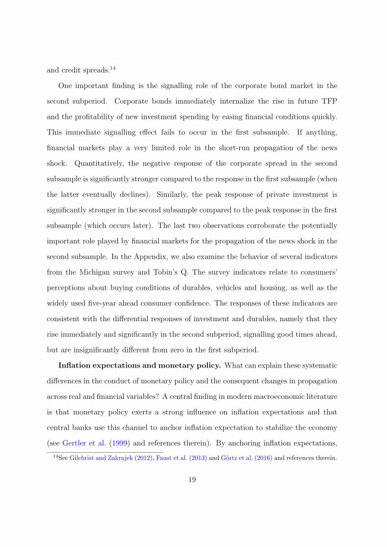
One important finding is the signalling role of the corporate bond market in the

second subperiod. Corporate bonds immediately internalize the rise in future TFP

and the profitability of new investment spending by easing financial conditions quickly.

This immediate signalling effect fails to occur in the first subsample. If anything,

financial markets play a very limited role in the short-run propagation of the news

shock. Quantitatively, the negative response of the corporate spread in the second

subsample is significantly stronger compared to the response in the first subsample (when

the latter eventually declines). Similarly, the peak response of private investment is

significantly stronger in the second subsample compared to the peak response in the first

subsample (which occurs later). The last two observations corroborate the potentially

important role played by financial markets for the propagation of the news shock in the

second subsample. In the Appendix, we also examine the behavior of several indicators

from the Michigan survey and Tobin’s Q. The survey indicators relate to consumers’

perceptions about buying conditions of durables, vehicles and housing, as well as the

widely used five-year ahead consumer confidence. The responses of these indicators are

consistent with the differential responses of investment and durables, namely that they

rise immediately and significantly in the second subperiod, signalling good times ahead,

but are insignificantly different from zero in the first subperiod.

Inflation expectations and monetary policy. What can explain these systematic

differences in the conduct of monetary policy and the consequent changes in propagation

across real and financial variables? A central finding in modern macroeconomic literature

is that monetary policy exerts a strong influence on inflation expectations and that

central banks use this channel to anchor inflation expectation to stabilize the economy

(see Gertler et al. (1999) and references therein). By anchoring inflation expectations,

14See Gilchrist and Zakrajek (2012), Faust et al. (2013) and Gortz et al. (2016) and references therein.

19

IRF of INVESTMENT

10 20 30 40 50 60-0.03

-0.02

-0.01

0

0.01

0.02

0.03IRF of CONS. DURABLES

10 20 30 40 50 60-0.02

-0.015

-0.01

-0.005

0

0.005

0.01

0.015IRF of REAL 3M RATE

10 20 30 40 50 60-0.1

0

0.1

0.2

0.3

0.4

0.5

0.6

0.7IRF of BAA-AAA SPREAD

10 20 30 40 50 60-0.08

-0.06

-0.04

-0.02

0

0.02

0.04

0.06

Figure 7: First sample (1954:Q3-1979:Q2). The solid line is the median estimated impulseresponse (in percent) to a positive TFP news shock. Shaded areas indicate the 16% and84% confidence bands.

IRF of INVESTMENT

10 20 30 40 50 600

0.005

0.01

0.015

0.02

0.025

0.03

0.035

0.04IRF of CONS. DURABLES

10 20 30 40 50 600

0.005

0.01

0.015

0.02

0.025

0.03

0.035IRF of REAL 3M RATE

10 20 30 40 50 60-0.2

-0.1

0

0.1

0.2

0.3

0.4IRF of BAA-AAA SPREAD

10 20 30 40 50 60-0.2

-0.15

-0.1

-0.05

0

0.05

Figure 8: Second sample (1982:Q3-2013:Q4). The solid line is the median estimatedimpulse response (in percent) to a positive TFP news shock. Shaded areas indicate the16% and 84% confidence bands.

the monetary authority retains control on current inflation without having to aggressively

adjust the policy rate. These theoretical insights provide a powerful metric to detect

systematic variations in the conduct of monetary policy across subperiods. To the

extent that large and persistent movements in inflation cannot occur without substantial

changes in monetary policy, we can glean information about variations in the conduct

of monetary policy from the differences in the responses of inflation and inflation

expectations to anticipated changes in TFP.

Figures 9 and 10 show the responses of current inflation and expected inflation—

measured by the one-year-ahead inflation expectations from the Michigan Survey of

Consumers—to the TFP news shock before and after 1980, respectively. It also

displays the IRFs of activity indicators and the Fed Funds rate. Two observations

stand out. First, the responses of inflation expectations across the two subperiods are

20

remarkably different. In the first subperiod, inflation expectations exhibit a decline

in the short run similarly, although smaller in magnitude, to the decline in realised

inflation. However, shortly after this decline, inflation expectations rise, suggesting that

the public expects inflation to rise. Interestingly, the rise in inflation expectations occurs

while realized inflation is still declining (at the 10-quarter horizon). The rise in inflation

expectations coincides with the peak in economic activity, which occurs at the 10-quarter

horizon. Inflation expectations remain consistently high thereafter; as long as activity

remains strong (see the response of output), consumers seem to expect higher inflation.

Interestingly, they seem to expect higher inflation permanently even as the economic

boom subsides in the long run. This finding is interesting since it involves a concurrent

increase in TFP, which could, with other things being equal, keep inflationary pressures

in check. By contrast, in the second subperiod, expected inflation shows a small and

persistent decline that returns to the initial state gradually while the actual inflation

response has returned to zero by around the two-year horizon. The interesting finding

in the second subperiod compared to the first one is that inflation expectations are

decoupled from the boom in economic activity that is strong and immediate following

the news TFP shock. Clearly, in the second subperiod, future growth in TFP is perceived

as being disinflationary.

Changes in the conduct of monetary policy. To better understand these

markedly different results across subperiods, it is important to relate the findings to

the broader historical context of the conduct of monetary policy in the United States.

The first subperiod broadly coincides with the term of governor William McChesney

Martin, chairman of the Board of Governors of the Federal Reserve from April 1951 to

January 1970. During this period, the Fed used independence gained with the Treasury-

Fed Accord to begin a new regime for monetary policy, which chairman Martin described

as “leaning against the wind.” During this period, the FOMC began to use systematic

21

IRF of TFP

10 20 30 40 50 60-0.005

0

0.005

0.01

0.015

0.02

0.025IRF of OUT

10 20 30 40 50 60

×10-3

-5

0

5

10

15IRF of CONS

10 20 30 40 50 600

0.002

0.004

0.006

0.008

0.01

IRF of HRS

10 20 30 40 50 60

×10-3

-4

-2

0

2

4

6

8IRF of INFLATION

10 20 30 40 50 60

×10-3

-8

-6

-4

-2

0

2IRF of FED FUNDS

10 20 30 40 50 60

×10-3

-4

-2

0

2

4

IRF of E(INFLATION)

10 20 30 40 50 60-0.4

-0.3

-0.2

-0.1

0

0.1

0.2

Figure 9: First sample (1954:Q3-1979:Q2). The solid line is the median estimated impulseresponse (in percent) to a positive TFP news shock from a seven variable VAR featuringTFP, output, consumption, hours, inflation, Fed Funds rate, and one-year-ahead Michiganinflation expectations estimated with four lags. Shaded areas indicate the 16% and 84%confidence bands.

22

IRF of TFP

10 20 30 40 50 60

×10-3

-5

0

5

10

15

20IRF of OUT

10 20 30 40 50 600

0.002

0.004

0.006

0.008

0.01IRF of CONS

10 20 30 40 50 60

×10-3

0

2

4

6

8

IRF of HRS

10 20 30 40 50 60

×10-3

-5

0

5

10IRF of INFLATION

10 20 30 40 50 60

×10-3

-5

-4

-3

-2

-1

0

1IRF of FED FUNDS

10 20 30 40 50 60

×10-3

-3

-2

-1

0

1

2

IRF of E(INFLATION)

10 20 30 40 50 60-0.4

-0.3

-0.2

-0.1

0

0.1

Figure 10: Second sample (1982:Q3-2013:Q4). The solid line is the median estimatedimpulse response (in percent) to a positive TFP news shock from a seven variable VARfeaturing TFP, output, consumption, hours, inflation, Fed Funds rate, and one-year-aheadMichigan inflation expectations estimated with four lags. Shaded areas indicate the 16%and 84% confidence bands.

23

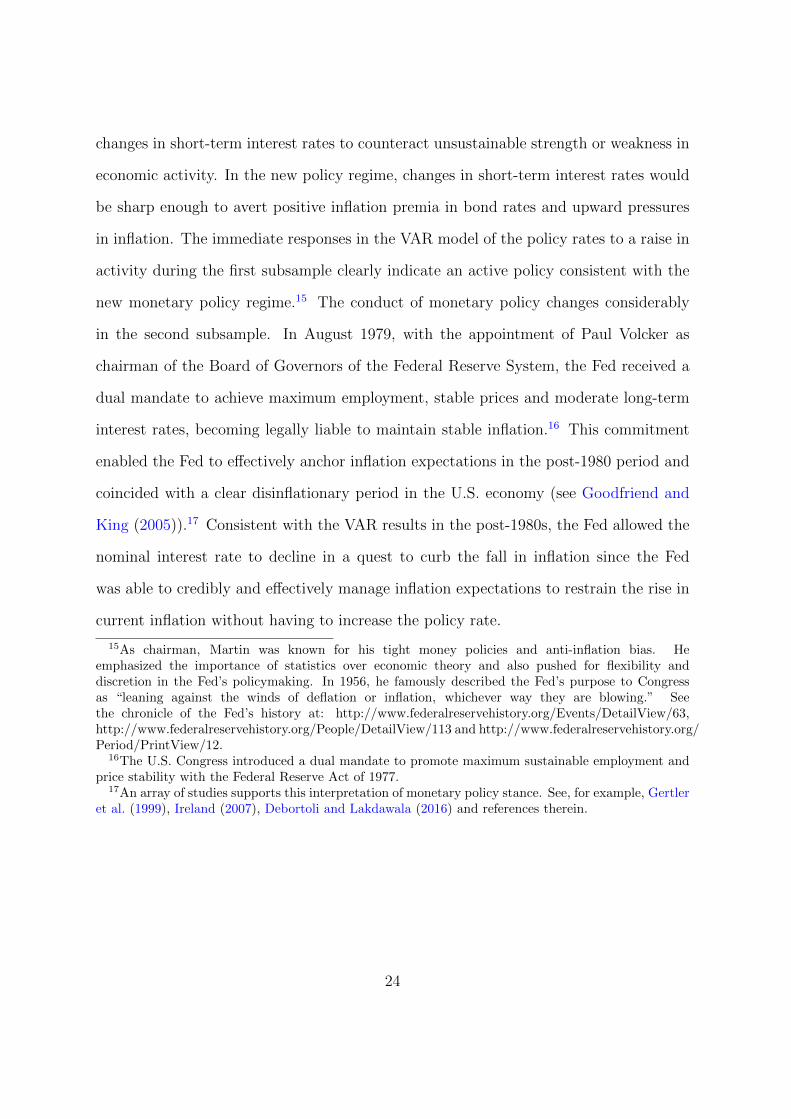
changes in short-term interest rates to counteract unsustainable strength or weakness in

economic activity. In the new policy regime, changes in short-term interest rates would

be sharp enough to avert positive inflation premia in bond rates and upward pressures

in inflation. The immediate responses in the VAR model of the policy rates to a raise in

activity during the first subsample clearly indicate an active policy consistent with the

new monetary policy regime.15 The conduct of monetary policy changes considerably

in the second subsample. In August 1979, with the appointment of Paul Volcker as

chairman of the Board of Governors of the Federal Reserve System, the Fed received a

dual mandate to achieve maximum employment, stable prices and moderate long-term

interest rates, becoming legally liable to maintain stable inflation.16 This commitment

enabled the Fed to effectively anchor inflation expectations in the post-1980 period and

coincided with a clear disinflationary period in the U.S. economy (see Goodfriend and

King (2005)).17 Consistent with the VAR results in the post-1980s, the Fed allowed the

nominal interest rate to decline in a quest to curb the fall in inflation since the Fed

was able to credibly and effectively manage inflation expectations to restrain the rise in

current inflation without having to increase the policy rate.

15As chairman, Martin was known for his tight money policies and anti-inflation bias. Heemphasized the importance of statistics over economic theory and also pushed for flexibility anddiscretion in the Fed’s policymaking. In 1956, he famously described the Fed’s purpose to Congressas “leaning against the winds of deflation or inflation, whichever way they are blowing.” Seethe chronicle of the Fed’s history at: http://www.federalreservehistory.org/Events/DetailView/63,http://www.federalreservehistory.org/People/DetailView/113 and http://www.federalreservehistory.org/Period/PrintView/12.

16The U.S. Congress introduced a dual mandate to promote maximum sustainable employment andprice stability with the Federal Reserve Act of 1977.

17An array of studies supports this interpretation of monetary policy stance. See, for example, Gertleret al. (1999), Ireland (2007), Debortoli and Lakdawala (2016) and references therein.

24

4 Conclusion

This paper documents significant changes in the effect of TFP news shocks on

macroeconomic variables before and after 1980. Short- and long-term nominal interest

rates exhibit a sign reversal in response to a news TFP shock before and after 1980. Using

the Expectations Hypothesis, which conveys a broad appraisal on the overall expected

stance of monetary policy, we document that the sign reversal also is echoed in the term

structure of expected policy rates across subperiods. Specifically, our empirical analysis

shows that the expectations component of long-term rates rises persistently in response

to the anticipated increase in TFP in the pre-1980 period, and it declines persistently in

the post-1980 period, suggesting a restrictive (accommodative) monetary policy stance

in the pre-1980 (post-1980) period in response to the news TFP shock. Several activity

variables also differ in their responses to the news shock across subperiods.

The analysis suggests that the different responses of macroeconomic aggregates to

news shocks between subperiods are related to sharp changes in the conduct of monetary

policy. Systematic policy changes are reflected by the ineffectiveness of the Fed to anchor

inflation expectations in the pre-1980 period and the subsequent strong objective to

achieve stable inflation that leads to a powerful anchoring of inflation expectations in

the post-1980 period. Thus, the Fed’s weak influence over the formation of expectations

in the first subperiod leads to a tightening of monetary policy in response to any initial

increase in economic activity in consequence of the news shock. By contrast, the Fed

adopts a loosening monetary policy in the second subperiod since it can credibly and

effectively manage inflation expectations to restrain the rise in inflation that results from

the increase in real activity generated by the news shock.

Our study offers several interesting directions for future research. It would certainly

be valuable to develop structural models to study the interaction between the formation

25

of expectations and systematic changes in the conduct of monetary policy, which is

a central finding of our analysis. Such models should incorporate imperfect common

knowledge of economic agents that recent studies find capable of generating a reversal

in the response of the economy to aggregate disturbances.18 Disperse information is also

a critical feature to include in the model since it may interact with monetary policy to

explain changes in the propagation of anticipated news shocks, as Melosi (2014) shows

for the propagation of monetary and technology shocks. These important extensions

remain open to future research.

18See Melosi (2016) and references therein for a recent discussion of the issues.

26

References

Barsky, R. B., Basu, S., and Lee, K. (2015). Whither News Shocks? NBER

Macroeconomics Annual, 29(1):225 – 264.

Barsky, R. B. and Sims, E. R. (2011). News shocks and business cycles. Journal of

Monetary Economics, 58(3):273–289.

Basu, S., Fernald, J., Fisher, J., and Kimball, M. (2010). Sector specific technical change.

Mimeo.

Basu, S., Fernald, J., and Kimpball, M. (2006). Are technology improvements

contractionary? American Economic Review, 96(5):1418–1448.

Beaudry, P. and Portier, F. (2004). An exploration into Pigou’s theory of cycles. Journal

of Monetary Economics, 51(6):1183–1216.

Beaudry, P. and Portier, F. (2006). News, stock prices and economic fluctuations. The

American Economic Review, 96(4):1293–1307.

Beaudry, P. and Portier, F. (2014). News-Driven Business Cycles: Insights and

Challenges. Journal of Economic Literature, 52(4):993–1074.

Ben Zeev, N. and Khan, H. (2015). Investment Specific News Shocks and U.S. Business

Cycles. Journal of Money, Credit and Banking, 47(7):1443–1464.

Benati, L. (2004). Evolving post World War II U.K. economic performance. Journal of

Money, Credit and Banking, 36(1):pp. 691–717.

Bianchi, F., Mumtaz, H., and Surico, P. (2009). The Great Moderation of the term

structure of UK interest rates. Journal of Monetary Economics, 56(6):856–871.

27

Boivin, J. and Giannoni, M. P. (2006). Has Monetary Policy Become More Effective?

The Review of Economics and Statistics, 88(3):445–462.

Castelnuovo, E. (2012). Estimating the Evolution of Moneys Role in the U.S. Monetary

Business Cycle. Journal of Money, Credit and Banking, 44(1):23–52.

Christiano, L. J., Ilut, C., Motto, R., and Rostagno, M. (2010). Monetary policy and

stock market booms. Proceedings Economic Policy Symposium Jackson Hole, pages

85–145.

Clarida, R., Gal, J., and Gertler, M. (2000). Monetary policy rules and macroeconomic

stability: evidence and some theory. Quarterly Journal of Economics, 115:147–180.

Debortoli, D. and Lakdawala, A. (2016). How Credible Is the Federal Reserve? A

Structural Estimation of Policy Re-optimizations. American Economic Journal:

Macroeconomics, 8(3):42–76.

Faust, J., Gilchrist, S., Wright, J. H., and Zakrajssek, E. (2013). Credit spreads

as predictors of real-time economic activity: a Bayesian model-averaging approach.

Review of Economics and Statistics, 95(5):1501–1519.

Fernald, J. (2012). A quarterly, utilization–adjusted series on total factor productivity.

Working Paper, (2012-19).

Forni, M., Gambetti, L., and Sala, L. (2014). No News in Business Cycles. Economic

Journal, 124(581):1168–1191.

Fujiwara, I., Hirose, Y., and Shintani, M. (2011). Can news be a major source of

aggregate fluctuations? A Bayesian DSGE approach. Journal of Money, Credit and

Banking, 43(1):1–29.

28

Gambetti, L. and Gali, J. (2009). On the Sources of the Great Moderation. American

Economic Journal: Macroeconomics, 1(1):26–57.

Gertler, M., Gali, J., and Clarida, R. (1999). The Science of Monetary Policy: A New

Keynesian Perspective. Journal of Economic Literature, 37(4):1661–1707.

Gilchrist, S. and Zakrajek, E. (2012). Credit spreads and business cycle fluctuations.

American Economic Review, 102(4):1692–1720.

Gilchrist, S. and Zakrajsek, E. (2012). Credit spreads and business cycle fluctuations.

American Economic Review, 102(4):1692–1720.

Goodfriend, M. and King, R. G. (2005). The incredible Volcker disinflation. Journal of

Monetary Economics, 52(5):981–1015.

Gortz, C. and Tsoukalas, J. (2017). News and financial intermediation in aggregate

fluctuations. Review of Economics and Statistics, 99:514–530.

Gortz, C., Tsoukalas, J. D., and Zanetti, F. (2016). News Shocks under Financial

Frictions. Economics Series Working Papers 813, University of Oxford, Department

of Economics.

Ireland, P. N. (2000). Interest Rates, Inflation, and Federal Reserve Policy since 1980.

Journal of Money, Credit and Banking, 32(3):417–434.

Ireland, P. N. (2003). Endogenous money or sticky prices? Journal of Monetary

Economics, 50(8):1623–1648.

Ireland, P. N. (2007). Changes in the Federal Reserve’s Inflation Target: Causes and

Consequences. Journal of Money, Credit and Banking, 39(8):1851–1882.

29

Karnizova, L. (2010). The spirit of capitalism and expectation-driven business cycles.

Journal of Monetary Economics, 57(6):739–752.

Kurmann, A. and Otrok, C. (2013). News shocks and the slope of the term structure of

interest rates. American Economic Review, 103:2612–2632.

Liu, P., Mumtaz, H., Theodoridis, K., and Zanetti, F. (2017). Changing Macroeconomic

Dynamics at the Zero Lower Bound. Economics Series Working Papers 824, University

of Oxford, Department of Economics.

Melosi, L. (2014). Estimating models with dispersed information. American Economic

Journal: Macroeconomics, 6(1):1–31.

Melosi, L. (2016). Signalling effects of monetary policy. The Review of Economic Studies,

84(2):853–884.

Milani, F. (2011). Expectation shocks and learning as drivers of the business cycle. The

Economic Journal, 121(552):379–401.

Mumtaz, H. and Surico, P. (2012). Evolving International Inflation Dynamics: World

And Country-Specific Factors. Journal of the European Economic Association,

10(4):716–734.

Neville, F., Owyang, M., Roush, J., and DiCecio, R. (2014). A flexible finite-horizon

alternative to long-run restrictions with an application to technology shocks. Review

of Economics and Statistics, 96:638–647.

Pigou, A. C. (1926). Industrial Fluctuations. Macmillan. London.

Schmitt-Grohe, S. and Uribe, M. (2012). What’s news in business cycles? Econometrica,

80(6):2733–2764.

30

Svensson, L. E. (2010). Inflation Targeting. In Friedman, B. M. and Woodford,

M., editors, Handbook of Monetary Economics, volume 3 of Handbook of Monetary

Economics, chapter 22, pages 1237–1302. Elsevier.

Taylor, J. B. (1993). Discretion versus policy rules in practice. Carnegie-Rochester

Conference Series on Public Policy, 39(1):195–214.

Theodoridis, K. and Zanetti, F. (2016). News shocks and labour market dynamics in

matching models. Canadian Journal of Economics, 49(3):906–930.

Uhlig, H. (2004). What moves GNP? Econometric Society 2004 North American Winter

Meetings 636, Econometric Society.

31

Appendix

A Data Sources and Time Series Construction

Table 1 provides an overview of the data used in the analysis. Below we describe

in detail all of the data transformations we made to construct the dataset for the

estimation of the VAR model. We take the data series for aggregate utilization adjusted

TFP to estimate the VARs from John Fernald’s website (www.frbsf.org/economic −

research/economists/jfernald/quarterly tfp.xls), as described in Fernald (2012).

Table 1: Time Series used in the empirical analysis

Time Series Description Units Code Source

Gross domestic product CP, SA, billion $ GDP BEAGross Private Domestic Investment CP, SA, billion $ GPDI BEAReal Gross Private Domestic Investment CVM, SA, billion $ GPDIC1 BEAPersonal Consumption Exp.: Durable Goods CP, SA, billion $ PCDG BEAReal Personal Consumption Exp.: Durable Goods CVM, SA, billion $ PCDGCC96 BEAPersonal Consumption Expenditures: Services CP, SA, billion $ PCESV BEAReal Personal Consumption Expenditures: Services CVM, SA, billion $ PCESVC96 BEAPersonal Consumption Exp.: Nondurable Goods CP, SA, billion $ PCND BEAReal Personal Consumption Exp.: Nondurable Goods CVM, SA, billion $ PCNDGC96 BEACivilian Noninstitutional Population NSA, 1000s CNP160V BLSNon-farm Business Sector: Compensation Per Hour SA, Index 2005=100 COMPNFB BLSNon-farm Business Sector: Hours of All Persons SA, Index 2005=100 HOANBS BLSEffective Federal Funds Rate NSA, percent FEDFUNDS BG3 Month Treasury Bill Rate NSA T-Bill St. Louis FED FRED1 Year, 5 Year, 10 Year government bond Yields NSA Fed BoardAll Employees SA B-1 BLSAverage Weekly Hours SA B-7 BLSE5Y Confidence Indicator Table 29 Michigan SurveyBuy Intentions Durables Table 35 Michigan SurveyBuy Intentions Vehicles 1 Year ahead Table 37 Michigan SurveyBuy Conditions Housing Table 41 Michigan SurveyBAA-AAA corporate spread St. Louis FED FRED

CP = current prices, CVM = chained volume measures (2005 Dollars), SA = seasonally adjusted, NSA = not seasonallyadjusted. BEA = U.S. Department of Commerce: Bureau of Economic Analysis, BLS = U.S. Department of Labor: Bureau ofLabor Statistics and BG = Board of Governors of the Federal Reserve System, IEC = Federal Financial Institutions ExaminationCouncil, FRB = Federal Reserve Board.

Real and nominal variables. Consumption (in current prices) is defined as

32

the sum of personal consumption expenditures on services and personal consumption

expenditures on non-durable goods. The time series for real consumption is constructed

as follows. First, we compute the shares of services and non-durable goods in total

(current price) consumption. Then, total real consumption growth is obtained as the

chained weighted (using the nominal shares above) growth rate of real services and

growth rate of real non-durable goods. Using the growth rate of real consumption, we

construct a series for real consumption using 2005 as the base year. The consumption

deflator is calculated as the ratio of nominal over real consumption. In the VAR model,

we use the log change in the GDP deflator as our inflation measure; however results are

nearly identical when we use the consumption deflator or CPI inflation. Analogously, we

construct a time series for the investment deflator using series for (current price) personal

consumption expenditures on durable goods and gross private domestic investment

and chain weight to arrive at the real aggregate. Real output is GDP expressed in

consumption units by dividing current price GDP with the consumption deflator.

The hourly wage is defined as total compensation per hour. Dividing this series by

the consumption deflator yields the real-wage rate. Hours worked is given by hours of

all persons in the non-farm business sector. All series described above are expressed in

per capita terms using the series of non-institutional population, age 16 and above.

The BAA-AAA spread. The spread is obtained from the Federal Reserve Bank

of St. Louis’ online database FRED (https : //fred.stlouisfed.org.).

Tobin’s Q. Tobin’s Q is the ration of market to book value for the Dow Jones

Industrial Average. This definition is taken directly from Welsh and Goyal (2008), “A

Comprehensive Look at The Empirical Performance of Equity Premium Prediction,”

Review of Financial Studies, 21.

33

B Specification for the Minnesota prior in the VAR

Assume the simple VAR(p) model

yt = v + A1yt−1 + ...+ Apyt−p + εt, (2)

where yt is a n× 1 vector of variables, and εt ∼ N (0,Σ) with Σ the covariance matrix.

The prior for the VAR coefficients A =[v, A′1, ..., A

′p

]′is of the form

vec (A) ∼ N(β, V

),

where β is one for variables that are in log-levels, and zero for rate variables (inflation,

short and long interest rates). The prior variance V is diagonal with elements,

V i,jj =

a1p2

for coefficients on own lags

a2σiip2σjj

for coefficients on lags of variable j 6= i

a3σii for intercepts

. (3)

where, p denotes the number of lags. Here σii is the residual variance from the

unrestricted p-lag univariate autoregression for variable i. The degree of shrinkage

depends on the hyperparameters a1, a2, a3. We set a3 = 100, and we select a1, a2 by

specifying a wide grid of possible values19. We take all possible pairs of a1 and a2 on

these grids, thus, estimating 1540 models with varying degrees of prior informativeness.

The optimal shrinkage pair for a1 and a2 is the one that maximizes the in-sample fit of

the VAR, as measured by the Bayesian Information Criterion. The covariance matrix

has a diffuse prior of the form p(Σ) ∝ |Σ|−(n+1)/2.

19The grids of values we use are: a1 = (1e-5,2e-5,3e-5,4e-5,5e-5,6e-5,7e-5,8e-5,9e-5,1e-4,2e-4,3e-4,4e-4,5e-4,6e-4,7e-4,8e-4,9e-4,0.001,0.002,0.003,0.004,0.005,0.006,0.007,0.008,0.009,0.01,0.02,0.03,0.04,0.05,0.06,0.07,0.08,0.09,0.1,0.2,0.3,0.4,0.5,0.6,0.7,0.8,0.9,1,2,3,4,5,6,7,8,9,10),a2 = (0.01,0.02,0.03,0.04,0.05,0.06,0.07,0.08,0.09,0.1,0.2,0.3,0.4,0.5,0.6,0.7,0.8,0.9,1,2,3,4,5,6,7,8,9,10).

34

C Forward-looking variables

Do responses to forward-looking variables across the two sub-samples show any

systematic change related to the variation in the responses of series of economic activity

and interest rates? Figures 11 and 12 show the responses of several expectation indicators

from the Michigan Survey of Consumers and Tobin’s Q. Tobin’s Q refers to the ratio of

market value to book value of companies in the Dow Jones Industrial average, and it is

a key forward-looking measure of how financial markets assess profitability in modern

investment theory. In the first subperiod, the response of consumer confidence (E5Y)

is insignificant on impact, only becoming significantly positive after one year. In the

second subperiod, by contrast, the response of consumer confidence is strongly and

persistently positive at all horizons, suggesting confidence about expansionary prospects

of the economy. This response is interesting despite some delay in the rise of TFP

(not shown here). We examine the behavior of three other confidence indicators from

the Michigan survey that are highly representative of the consumers’ perception about

future economic conditions, namely buying conditions for consumer durables, housing

and vehicles. In the first subperiod, none of the responses of buying conditions for

consumer durables, housing or vehicles is significantly different from zero. By contrast,

in the second subperiod, the responses are strongly positive and significant, suggesting

that consumers perceive good times ahead. The response of Tobin’s Q also is quite

different quantitatively across subperiods. Tobin’s Q is a key summary statistic for

private investment spending because it incorporates future expectations about corporate

profitability and captures how the stock market values capital of the corporate sector.

While the response of the Tobin’s Q is qualitatively similar across horizons in both

subperiods, the response in the first subperiod is insignificant on impact. By contrast,

the response in the second subperiod is approximately four times larger than the first

35

subperiod.

IRF of E5Y

10 20 30 40 50 60-0.03

-0.02

-0.01

0

0.01

0.02

0.03

0.04IRF of DURABLES BUY CONDITIONS

10 20 30 40 50 60-5

-4

-3

-2

-1

0

1

2IRF of VEHICLES 1 YEAR AHEAD CONDITIONS

10 20 30 40 50 60-6

-4

-2

0

2

4

IRF of HOUSES BUY CONDITIONS

10 20 30 40 50 60-6

-4

-2

0

2

4IRF of TOBINS Q

10 20 30 40 50 60-0.02

0

0.02

0.04

0.06

0.08

Figure 11: First sample (1954:Q3-1979:Q2)–Michigan surveys and Tobin’s Q. The solidline is the median estimated impulse response (in percent) to a positive TFP news shock.Shaded areas indicate the 16% and 84% confidence bands.

36

IRF of E5Y

10 20 30 40 50 60-0.01

0

0.01

0.02

0.03

0.04IRF of DURABLES BUY CONDITIONS

10 20 30 40 50 60-1

0

1

2

3

4IRF of VEHICLES 1 YEAR AHEAD CONDITIONS

10 20 30 40 50 60-1

0

1

2

3

4

5

IRF of HOUSES BUY CONDITIONS

10 20 30 40 50 60-1

0

1

2

3

4

5

6IRF of TOBINS Q

10 20 30 40 50 60-0.05

0

0.05

0.1

0.15

0.2

0.25

0.3

Figure 12: Second sample (1982:Q3-2013:Q4)–Michigan surveys and Tobin’s Q. The solidline is the median estimated impulse response (in percent) to a positive TFP news shock.Shaded areas indicate the 16% and 84% confidence bands.

37