Housing and the Macroeconomy: The Role of ImplicitGuarantees for Government Sponsored Enterprises∗

Karsten JeskeFederal Reserve Bank of Atlanta

Dirk KruegerUniversity of Pennsylvania, CEPR and NBER

March 28, 2007

Abstract

This paper studies the macroeconomic effects of implicit government bailout guaranteesof debt obligations of Government-Sponsored Enterprises such as Fannie Mae and FreddyMac. We construct a model with heterogenous infinitly lived households and competitivehousing and mortgage markets where the government provides households with a mortgageinterest rate subsidy. We use this model to evaluate the aggregate and distributional impactsof this government subsidy to home owners. We find that eliminating the interest ratesubsidy leads to lower equilibrium housing investment, substantially lower mortgage defaultrates and higher aggregate welfare. The welfare effects of removing the subsidy, however,vary substantially across members of the population with different economic characteristics.Keywords: Housing, Mortgage Market, Default RiskJEL codes: E21, G11, R21

∗The authors can be reached at Karsten.Jeske@atl.frb.gov and dkrueger@econ.upenn.edu. We have benefitedfrom helpful comments by seminar participants at the Wharton macro lunch, the Banco de Espana, The HousingConference at the Bank of Canada and the Federal Reserve Bank of Atlanta. Part of this paper was completedwhile Krueger was a research visitor at the European Central Bank

1 Introduction

With close to 70% the United States displays one of the highest home ownership ratios in theworld. Part of the attractiveness of owner-occupied housing stems from a variety of subsidies thegovernment provides to homeowners. Apart from direct subsidies to low-income households viaHUD (need to write this out or explain) programs, three important indirect subsidies exist. Thefirst - and most well known - is the fact that mortgage interest payments (of mortgages up to $1million) are tax-deductible. Second, the implicit income from housing capital (i.e. the imputedrental-equivalent) is not taxable, while other forms of capital income (e.g. interest, dividend andcapital gains income) are being taxed. Gervais (2001) addresses the adverse effects of these twosubsidies within a general equilibrium life-cycle model.The third subsidy arises from the special structure of the US mortgage market. Essentially

all home mortgages in the US are being sold from individual banks to so called GovernmentSponsored Enterprises (GSEs) who in turn refinance themselves via the bond market. A formi-dable summary of the institutional details surrounding GSEs can be found in Frame and Wall(2002a) and (2002b). The three most important GSE are the two privately owned and publiclytraded companies Fannie Mae (Federal National Mortgage Association) and Freddie Mac (Fed-eral Home Loan Mortgage Association), and the FHLB (Federal Home Loan Bank system), apublic and non-profit organization. The close link of GSEs to the federal government createsthe impression that the government provides a guarantee to GSEs shielding them from aggregaterisks, most notably aggregate credit risk which lowers their refinancing cost to below what privateinstitutions would have to pay. The purpose of this paper is to quantify the macroeconomic anddistributional effects of this subsidy; our paper is - to our knowledge - the first attempt to do sowithin a structural dynamic general equilibrium model.According to Frame andWall, GSEs enjoy an array of government benefits, for example being

exempt from state and federal income taxes, a line of credit with the Treasury Department andvery importantly a special status of GSE-issued debt. In particular, GSE securities can serve assubstitutes to government bonds for transactions between public entities that normally requireto be done in Treasuries. The Federal Reserve System also accepts GSE debt as a substitutefor Treasuries in their portfolio of repurchase agreements. While no written federal guaranteefor GSE debt exists, market participants view the special status of GSE debt as an indicationof an implicit guarantee making them almost as safe as Treasury bills. The perception of afederal guarantee is further fueled by the sheer size of the GSE mortgage portfolio amountingto about 3 trillion dollars, 2.4 trillion dollars of which coming from the larger two GSEs, FannieMae and Freddie Mac. Insolvency of any one or both of these companies, say, due to an adverseshock in the real estate market that increases aggregate mortgage delinquency, will cause majordisruptions in the financial system, which is why market participants consider housing GSEs tobe too large to fail. Finally, two previous government bailouts of housing GSEs - Fannie Mae inthe early 1980s and one of the smaller housing GSEs in the late 1980s - are further evidence thata bailout is likely should housing GSEs get into financial trouble.The implicit federal guarantee is more than mere perception; most importantly, it is reflected

in interest rates GSEs pay when borrowing. GSEs can borrow at rates only marginally higherthan the Treasury but about 40 basis points lower than private companies without a governmentguarantee, according to the Congressional Budget Office CBO (2001). This is despite the fact thatGSEs are highly leveraged entities with an equity cushion of only about 3% of their obligations,

1

much lower than the 8.45% in the thrift industry (figures taken from Frame and Wall (2002a)).To the extend that part of the interest advantage of GSEs is passed through to homeowners,there exists a subsidy from the federal government to homeowners.In order to assess the macroeconomic and distributional effects of this subsidy we construct

a heterogeneous agent general equilibrium model with incomplete markets in the tradition ofBewley (1986) and Aiyagari (1994). We add a real estate sector and mortgages, i.e., we allowhouseholds to borrow against their real estate wealth. We also explicitely model mortgage default.In the model we approximate the implicit bailout guarantee with a tax-financed direct subsidy tomortgage interest rates. Our economy would then corrspond to a world in which the governmenttaxes income every period and either saves the proceeds in an effort to smooth out the spendingshock of a potential insolvency of the GSEs, or alternatively, is able to buy insurance fromthe outside world via, say, a market for credit derivatives. Thus, in our model economy thegovernment subsidizes home ownership by reducing effective mortgage interest rates.Notice that it is not clear a priori that this subsidy has negative welfare consequences. This

is due to a second-best argument because our economy has incomplete markets. Specifically,lowering the borrowing cost through a subsidy will reduce the severity of the borrowing constraintof agents with adverse idiosyncratic shocks.Our results can be described as follows. First, the subsidy leads to an increase in investment

in housing assets and an increase in the construction of real estate. Looking at the distributionof housing assets, the mortgage subsidy does not significantly change the share of householdswith positive holdings of real estate. This is because on the one hand the subsidy makes realestate ownership more attractive but on the other hand, through a general equilibrium effect,rental housing becomes cheaper, which discourages homeownership for low-income and low-assethouseholds.Using a steady state utilitarian social welfare functional we find that the aggregate welfare

implications of the subsidy are negative, in the order of 0.32% of consumption equivalent varia-tion. In addition to the adverse aggregate welfare effects the results also suggest that primarilyhouseholds with low wealth prefer to live in an economy without subsidy while high wealthhouseholds benefit strongly from it, indicating adverse distributional effects of the reform.1

The remainder of the paper is organized as follows. Section 2 introduces the model anddefines equilibrium in an economy with a housing and mortgage market. Section 3 characterizesequilibria. Section 4 describes the calibration of our economy. Section 5 details the numericalresults comparing two steady states in economies with and without a mortgage interest subsidy.Section 6 concludes the paper.

2 The Model

The endowment economy is populated by a continuum of measure one of infinitely lived house-holds, a continuum of competitive banks and a continuum of housing construction companies.Households face idiosyncratic endowment and housing depreciation shocks. In what follows wewill immediately proceed to describing the economy recursively, thereby skipping the (standard)sequential formulation of the economy.

1Gruber and Martin (2003) also study the distributional effects of the inclusion of housing wealth in a generalequilibrium model, but do not address the role of government housing subsidies for this question.

2

2.1 Households

Households have idiosyncratic endowment of the perishable consumption good given by y ∈ Y.These endowments follow a finite state Markov chain with transition probabilities π(y0|y) andunique invariant distribution Π(y).Households derive period utility U(c, h) from consumption and housing services h, which

can be purchased at a price pl (relative to the numeraire consumption good). In addition toconsumption and housing services the household can purchase two types of assets, one periodbonds b0 and houses g0. The price of bonds is denoted by Pb and the price of houses by Ph.Whereashouseholds cannot short-sell bonds, they can borrow against their real estate property. Let bym0 denote the size of their mortgage, and by Pm the receipt of resources (the consumption good)for each unit of mortgage issued and to be repaid tomorrow. These receipts will be determinedin equilibrium by competition of banks, and will depend on the characteristics of households aswell as the size of the mortgage m0 and size of the collateral g0. Houses depreciate stochastically;let F (δ0) denote the cumulative distribution function of the depreciation rate δ0 tomorrow, whichhas support D = [δ, δ]. Households possess the option of defaulting on their mortgages, at thecost of losing their housing collateral. They will choose to do so whenever

m0 > Ph(1− δ0)g0.

If there is a government bailout guarantee, then the government obtains general tax revenues bylevying proportional taxes τ on endowments. It will use the receipts from these taxes to bail outpart of the mortgages that private households have defaulted on. Finally let a denote cash athand, that is, after tax endowment plus receipts from all assets brought into the period.The individual state of a household consists of s = (a, y). Let the cross-sectional distribution

over individual states be given by μ. Since we will restrict our analysis to stationary equilibria inwhich μ is constant over time, in what follows the dependence of aggregate prices and quantitieson μ is left implicit.The dynamic programming problem of a household reads as

v(s) = maxc,h,b0,m0,g0≥0

(U(c, h) + β

Xy0

π(y0|y)Z δ

δ

v(s0)dF (δ0)

)(1)

s.t.c+ b0Pb + hPl + g0Ph −m0Pm (g

0,m0) = a+ g0Pl

a0(δ0, y0,m0, g0) = b0 +max{0, Ph(1− δ0)g0 −m0)}+ (1− τ)y0

Note that the budget constraint implies the timing convention that newly purchased real estateg0 can immediately be rented out in the same period. The function T describes the aggregatelaw of motion for the cross-sectional distribution over households’ characteristics.

2.2 The Real Estate Construction Sector

Firms in the real estate construction sector act competitively and face the linear technology

I = AhCh

3

where I is the output of houses of a representative firm, Ch is the input of the consumptiongood and Ah is a technological constant, measuring the amount of consumption goods requiredto build one house. For now we assume that this technology is reversible, that is, real estatecompanies can turn houses back into consumption goods using the same technology. Thus theproblem of a representative firm reads as

maxI,Ch

PhI − Ch (2)

s.t.

I = AhCh

Thus the equilibrium house price necessarily satisfies

Ph =1

Ah.

2.3 The Banking Sector

Let rb denote the risk free interest rate on one-period bonds, to be determined in general equilib-rium. Competitive banks take the refinancing costs Pb =

11+rb

as given. In addition we assumethat issuing mortgages is costly; let rw be the percentage real resource cost, per unit of mortgageissued, to the bank. This cost captures screening costs, administrative costs as well as mainte-nance costs of the mortgage (such as preparing and mailing a quarterly mortgage balance). Asa consequence, the effective net cost of the banking sector for financing one dollar of mortgage,equals rb + rw.Mortgage receipts Pm for a mortgage of sizem0 against real estate of size g0 are determined by

perfect competition in the banking sector, which implies that banks make zero expected profitsfor each mortgage they issue (as in Chatterjee et al. (2005)). Banks take account of the fact thathousehold may default on their mortgage, in which case the bank recovers the collateral valueof the house, which we assume to be a fraction γ ≤ 1 of the value of the real estate. For easeof exposition we assume that the cost of mortgage generation is paid not when the mortgage isissued, but when it repaid, which implies that households defaulting on their mortgage paymentsalso default on paying for the cost of generating the mortgage. Since this cost is fully priced intothe mortgage, this is equivalent to assuming that the resource cost of mortgage issue is due atthe receipt of the mortgage, but makes notation less cumbersome.In order to define a typical banks’ problem we first have to characterize the optimal default

choice of a household. The cut-off level of depreciation, above which a household defaults onher mortgage is given as follows.. Define as κ0 = m0

g0 the leverage (for g0 > 0) of a mortgage m0

backed by real estate g0. Then if the default cut-off δ∗(m0, g0) is in the interior of D = [δ, δ] it isgiven by

m0 = (1− δ∗(m0, g0))Phg0

and thus explicitly

δ∗(m0, g0) = δ∗(κ0) =

⎧⎪⎨⎪⎩δ if 1− κ0

Ph< δ

1− m0

g0Ph= 1− κ0

Phif 1− κ0

Ph∈ [δ, δ]

δ if 1− κ0

Ph> δ

4

Evidently a household that obtains a mortgage m0 > 0 without collateral, i.e. with g0 = 0defaults for sure. The receipt for this mortgage thus necessarily has to equal 0 as well, i.e.Pm(s, g

0 = 0,m0) = 0. For other types of mortgages (m0, g0) with m0 > 0 and g0 > 0, the banks’problem is to choose the price Pm (g

0,m0) to maximize

maxPm(g0,m0)

"−m0Pm (g

0,m0) +1

1 + rb + rw

(m0F (δ∗(κ0)) + γPhg

0Z δ

δ∗(κ0)

(1− δ0)dF (δ0)

)#

= m0 maxPm(g0,m0)

"−Pm (g

0,m0) +

µ1

1 + rb + rw

¶(F (δ∗(κ0)) +

γPh

κ0

Z δ

δ∗(κ0)

(1− δ0)dF (δ0)

)#(3)

In the presence of a government bailout, the government effectively subsidizes mortgages, informs to be specified below.

2.4 The Government

As stated above the government levies endowment taxes τ on households to subsidize mortgages.Subsidies take the form of direct interest rate subsidies.2

Define the interest rate on a mortgage with characteristics (m0, g0) as

rm (g0,m0) =

1

Pm (g0,m0)− 1

where Pm (g0,m0) is the mortgage pricing function without subsidy. Define as rm (g0,m0) and

Pm (s, g0,m0) the corresponding entities with subsidy. Since the subsidy is a mortgage interest

rate subsidy we model it as

rm (g0,m0) = rm (g

0,m0)− sub (g0,m0)

and thus

Pm (s, g0,m0) =

Pm (s, g0,m0)

1− sub (g0,m0) ∗ Pm (s, g0,m0)≥ Pm (s, g

0,m0)

The total subsidy for a mortgage of characteristics (s, g0,m0) is thus

sub (g0,m0) = m0³Pm (s, g

0,m0)− Pm (s, g0,m0)

´= m0Pm (s, g

0,m0)

µsub (g0,m0)Pm (s, g

0,m0)

1− sub (g0,m0)Pm (s, g0,m0)

¶and the total economy-wide subsidy is

Aggsub =

Zsub (g0,m0) dμ

Thus taxes have to satisfy

τ

Zydμ = Aggsub

τ =Aggsub

y(4)

where y is average (aggregate) endowment in the economy.2Other forms of mortgage subsidies can be easily mapped into these interest rate subsidies.

5

2.5 Equilibrium

We are now ready to define a stationary recursive Competitive Equilibrium. Let S = R+ × Ydenote the individual state space.

Definition 1 Given a government subsidy policy sub : R+×R+ → R, a Stationary RecursiveCompetitive Equilibrium are value and policy functions for the households, v, c, h, b0,m0, g0 :S → R, policies for the real estate construction sector I, Ch, prices functions Pl, Ph, Pb, mortgagepricing functions Pm, Pm : R+×R+ → R, a government tax rate τ and an invariant distributionμ such that

1. (Household Maximization) Given prices Pl, Ph, Pb, Pm and government policies the valuefunction solves (1) and c, h, b0,m0, g0 are the associated policy functions.

2. (Real Estate Construction Company Maximization) Given Ph, policies I, Ch solve (2).

3. (Bank Maximization) Given Ph, Pb, the function Pm solves (3)

4. (Government Budget Balance) The tax rate function τ satisfies (4), given the functionsm0, Pm, Pm, sub.

5. (Market Clearing in Rental Market)Zg0(s)dμ =

Zh(s)dμ

6. (Market Clearing in the Bond Market)Zb0(s)dμ =

Zm0(s)dμ

7. (Invariance of Distribution μ). The distribution μ is invariant with respect to the Markovprocess induced by the exogenous Markov process π and the policy functions m0, g0, b0.

When we derive the welfare consequences of removing the mortgage interest subsidy, wemeasure aggregate welfare via a Utilitarian social welfare function in the steady state, defined as

WEL =Z

v(s)μ(ds)

where μ is the invariant distribution.

3 Theoretical Results

In this section we state theoretical properties of our model the use of which makes the computa-tion of the model easier. These results consist of a characterization of the mortgage interest rate,a partial characterization of the solution to the household maximization problem and, finally,bounds on the equilibrium rental price Pl.

6

3.1 Mortgage Interest Rates

From equation (3) and the fact that competition requires profits for all mortgages issued inequilibrium to be zero we immediately obtain a characterization of equilibrium mortgage payoffsas

Pm (g0,m0) =

µ1

1 + rb + rw

¶(F (δ∗(m0, g0)) +

γPh

κ0

Z δ

δ∗(m0,g0)

(1− δ0)dF (δ0)

)

=

µ1

1 + rb + rw

¶(F (δ∗(κ0)) +

γ

Ahκ0

Z δ

δ∗(κ0)(1− δ0)dF (δ0)

)= Pm(κ

0)

with implied interest rates

rm(κ0) =

1

Pm(κ0)− 1

We note the following facts:

1. Mortgages are priced exclusively based on leverage κ0 = m0

g0 , that is Pm(m0, g0) = Pm(κ

0)where it is understood that the optimal choice of κ0 is a function of household characteristicss.

2. Pm(κ0) is decreasing in κ0, strictly so if the household defaults with positive probability.

Thus mortgage interest rates are increasing in leverage κ0.

3. Households that repay their mortgage with probability one have δ∗(κ0) = δ and thus

Pm(κ0) =

³1

1+rb+rw

´, i.e. they can borrow at the rate rb + rw.

4. Since for all δ0 > δ∗(κ0) we have γPhκ0(1−δ0) < 1, households that do default with positive

probability tomorrow receive Pm(κ0) <

³1

1+rb+rw

´today, that is, they borrow with a risk

premium rm(κ0) > rb + rw.

3.2 Simplification of the Household Problem

In the household problem define as

u(c;Pl) = maxc,h≥0

U(c, h)

s.t.

c+ Plh = c

Then the above problem can be rewritten as

v(s) = maxc,b0,m0,g0≥0

(u(c;Pl) + β

Xy0

π(y0|y)Z δ

δ

v(s0)dF (δ0)

)

s.t. c+ b0Pb + g0 [Ph − Pl]−m0Pm(κ0) = a

a0(δ0, h0,m0, g0) = b0 +max{0, Ph(1− δ0)g0 −m0)}+ (1− τ)y0

7

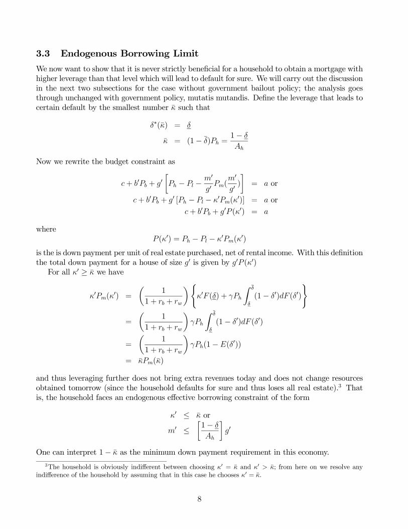
3.3 Endogenous Borrowing Limit

We now want to show that it is never strictly beneficial for a household to obtain a mortgage withhigher leverage than that level which will lead to default for sure. We will carry out the discussionin the next two subsections for the case without government bailout policy; the analysis goesthrough unchanged with government policy, mutatis mutandis. Define the leverage that leads tocertain default by the smallest number κ such that

δ∗(κ) = δ

κ = (1− δ)Ph =1− δ

Ah

Now we rewrite the budget constraint as

c+ b0Pb + g0∙Ph − Pl −

m0

g0Pm(

m0

g0)

¸= a or

c+ b0Pb + g0 [Ph − Pl − κ0Pm(κ0)] = a or

c+ b0Pb + g0P (κ0) = a

whereP (κ0) = Ph − Pl − κ0Pm(κ

0)

is the is down payment per unit of real estate purchased, net of rental income. With this definitionthe total down payment for a house of size g0 is given by g0P (κ0)For all κ0 ≥ κ we have

κ0Pm(κ0) =

µ1

1 + rb + rw

¶(κ0F (δ) + γPh

Z δ

δ

(1− δ0)dF (δ0)

)

=

µ1

1 + rb + rw

¶γPh

Z δ

δ

(1− δ0)dF (δ0)

=

µ1

1 + rb + rw

¶γPh(1−E(δ0))

= κPm(κ)

and thus leveraging further does not bring extra revenues today and does not change resourcesobtained tomorrow (since the household defaults for sure and thus loses all real estate).3 Thatis, the household faces an endogenous effective borrowing constraint of the form

κ0 ≤ κ or

m0 ≤∙1− δ

Ah

¸g0

One can interpret 1− κ as the minimum down payment requirement in this economy.

3The household is obviously indifferent between choosing κ0 = κ and κ0 > κ; from here on we resolve anyindifference of the household by assuming that in this case he chooses κ0 = κ.

8

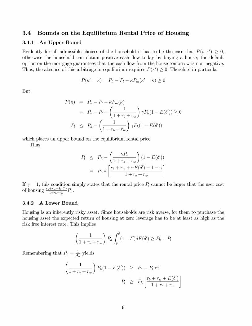
3.4 Bounds on the Equilibrium Rental Price of Housing

3.4.1 An Upper Bound

Evidently for all admissible choices of the household it has to be the case that P (s, κ0) ≥ 0,otherwise the household can obtain positive cash flow today by buying a house; the defaultoption on the mortgage guarantees that the cash flow from the house tomorrow is non-negative.Thus, the absence of this arbitrage in equilibrium requires P (κ0) ≥ 0. Therefore in particular

P (κ0 = κ) = Ph − Pl − κPm(κ0 = κ) ≥ 0

But

P (κ) = Ph − Pl − κPm(κ)

= Ph − Pl −µ

1

1 + rb + rw

¶γPh(1− E(δ0)) ≥ 0

Pl ≤ Ph −µ

1

1 + rb + rw

¶γPh(1−E(δ0))

which places an upper bound on the equilibrium rental price.Thus

Pl ≤ Ph −µ

γPh

1 + rb + rw

¶(1− E(δ0))

= Ph ∗∙rb + rw + γE(δ0) + 1− γ

1 + rb + rw

¸If γ = 1, this condition simply states that the rental price Pl cannot be larger that the user costof housing rb+rw+E(δ

0)1+rb+rw

Ph.

3.4.2 A Lower Bound

Housing is an inherently risky asset. Since households are risk averse, for them to purchase thehousing asset the expected return of housing at zero leverage has to be at least as high as therisk free interest rate. This impliesµ

1

1 + rb + rw

¶Ph

Z δ

δ

(1− δ0)dF (δ0) ≥ Ph − Pl

Remembering that Ph =1Ahyieldsµ1

1 + rb + rw

¶Ph(1−E(δ0)) ≥ Ph − Pl or

Pl ≥ Ph

∙rb + rw +E(δ0)

1 + rb + rw

¸

9

which states that the rental price of housing cannot be smaller than the (expected) user cost ofhousing in equilibrium (otherwise nobody would invest in housing, which cannot be an equilib-rium given strictly positive demand for housing services by consumers).4

In summary, what these theoretical results buy us, besides being interesting in its own right,is a simplified household problem, a concise characterization of the high-dimensional equilibriummortgage interest rate function and bounds for the equilibrium rental price, one of the endogenousprices to be determined in our analysis.

4 Calibration

4.1 Technology

Table 1: Technology Parameters

Parameter Interpretation Value TargetAh Technology Const. in Housing Constr. 1.0 none (normalized)π Transition Matrix for Income see below Tauchen ρ = 0.98, σe = 0.30y Income States see below Tauchen ρ = 0.98, σe = 0.30γ Foreclosure Technology 0.78 Pennington and Cross (2004)

Depreciation process see below BEA, OFHEO data

Housing Technology: We normalize the housing construction constant to Ah = 1.0, and thusthe price of one unit of housing to unity.

Income process: For a continuous state AR(1) process of the form

log y0 = ρ log y + (1− ρ2)0.5ε (5)

E (ε) = 0

E¡ε2¢= σ2e

we can calculate the unconditional standard deviation to be σe and the one-period autocorrelation(persistence) to be ρ. Estimates for ρ in the literature vary somewhat, but center around valuesclose to, but lower than 1. Motivated by the analysis by Storesletten et al. (2004) we selectρ = 0.98. The estimates for the standard deviation range from 0.2 to 0.4 (see Aiyagari (1994) fora discussion), so we choose σε = 0.3.

4With γ = 1 we thus immediately obtain that the rental price of housing Pl equals its user cost

Ph

hrb+rw+E(δ

0)1+rb+rw

i. In fact, what happens in this equilibrium is that households purchase houses, leverage such

that they default for sure tomorrow and the houses end up in the hand of the banks. Since these are risk-neutral,default is fully priced into the mortgage and banks receive the full (depreciated) value of the house, banks ratherthan households (which are risk averse) should and will end up owning the real estate.

10

We approximate the continuous state AR(1) with a 5 state Markov chain using the pro-cedure put forth by Tauchen and Hussey (1991). We get the five labor productivity shocksy ∈ {0.3586, 0.5626, 0.8449, 1.2689, 1.9909} and the following transition matrix:

Π =

⎡⎢⎢⎢⎢⎣0.7629 0.2249 0.0121 0.0001 0.00000.2074 0.5566 0.2207 0.0152 0.00010.0113 0.2221 0.5333 0.2221 0.01130.0001 0.0152 0.2207 0.5566 0.20740.0000 0.0001 0.0121 0.2249 0.7629

⎤⎥⎥⎥⎥⎦which generates the stationary distribution (0.1907, 0.2066, 0.2053, 0.2066, 0.1907) and averagelabor productivity of one.

Foreclosure technology: Pennington-Cross (2004) estimates the default loss parameter γ.This is done by looking at liquidation sales revenue from foreclosed houses and comparing it toa market price constructed via the OFHEO repeat sales index. He finds that on average the lossis 22%. The loss varies only slightly depending on the age of the loan, between 20% for loans16-20 months old to 26% for loans up to 10 months old, so it is safe to assume that in the modelγ = 0.78 for all loans.

The depreciation process: We calibrate the house value depreciation process to attain real-istic levels of default in the model while at the same generating the statistical properties of thehouse price appreciation and depreciation observed in the data.According to the Mortgage Banker Association (MBA (2006)), the quarterly foreclosure rate

has been about 0.4 percent in between 2000 and 2006. Abstracting from the possibility thatone house may go in and out of foreclosure multiple within one given year, this implies that onan annual basis, banks start foreclosure proceedings on about 1.6 percent of their mortgages.The ratio of mortgages in foreclosure that eventually end in liquidation was about 25 percentin 2005, according to MBA (2006). Most homeowners avoid liquidation by either selling theirproperty, refinancing their mortgage or just paying off the arrears. Consequently, only about 0.4percent of mortgages actually end in liquidation the way we model it here. Given the unusuallystrong home price appreciation over the past years, we view this figure as the lower bound onthe foreclosure rate and thus target a default rate of 0.5 percent.We target two data moments of depreciation, the mean and the standard deviation. The mean

depreciation for residential housing according to the Bureau of Economic Analysis was 1.48%between 1960 and 2002 (standard deviation 0.05%), computed as consumption of fixed capital inthe housing sector (Table 7.4.5) divided by the capital stock of residential housing. With regardsto the standard deviation of depreciation we utilize data from the Office of Federal HousingEnterprise Oversight (OFHEO). It models house prices as a diffusion process and estimateswithin-state and within-region annual house price volatility. The technical details can be foundin the paper by Calhoun (1996). The ballpark figure for the eight census regions is 9 − 10%volatility in the years 1998-2004. We use the upper bound σδ = 0.10 to account for the fact thatnationwide volatility is slightly higher than the within-region volatility.We found that using a log-normal distribution for the appreciation of real estate in our model,

i.e., log (1− δ) ∼ N (−μδ, σ2δ) with a mean and standard deviation above, does not generate a

11

sufficient share of foreclosures. Apparently, the right tail of the distribution is too thin. Inorder to get more realistic levels of mortgage default we incorporate a fatter right tail in thedistribution of δ. Specifically, we mix a log-normal distribution with a uniform distribution onδ ∈ [0, δmax] and assign a weight ωU to the Uniform part of the distribution. In other words, theprobability distribution function for depreciation is

f (δ) = (1− ωU)σ−1/2δ φ

µlog (1− δ) + μδ

σδ

¶+ ωUIδ∈[0,δmax]

1

δmax(6)

where φ is the pdf of a standard Normal distribution. We now have four parameters μδ, σ2δ, δ

max, ωU

to pin down three moments, the mean depreciation, the standard deviation and the share of mort-gages in default that the model generates. Because we have one degree of freedom we chose tofix σ2 = 0.08. Setting the remaining three parameters to

ωU = 0.0080

δmax = 0.8000

μδ = 0.0152

we exactly pin down V AR (log (1− δ)) = 0.10, E (δ) = 0.0148 and also attain a realistic shareof foreclosures of 0.55 percent, slightly above the lower bound of 0.40 percent derived above.

4.2 Preferences

Table 2: Preferencs Parameters

Parameter Interpretation Value Targetσ Risk Aversion 2.0000 standardβ Time Discount Factor 0.8870 Net Worth/Incomeθ Share Parameter on Nondur. Cons. 0.8590 Exp. Share in BEA Data

For the utility function we start with a CES functional form:

u (c, h) = (1− β)(θcν + (1− θ)hν)

1−σν − 1

1− σ

Notice that the first order conditions in the intratemporal optimization problem yield the con-dition

h

c=

µPl

θ

1− θ

¶ 1ν−1

which implies that in steady state θ and ν cannot be pinned down separately. We thereforechoose ν = 0, which reduces the period utility function to

u (c, h) =cθ(1−σ)h(1−θ)(1−σ) − 1

1− σ

12

which allows us to easily calibrate θ to the share of housing vs. non-housing consumption. Forthe CRRA parameter we pick σ = 2 as is standard in the literature. See, for example, Attanasio(1999) and Gourinchas and Parker (2002).The time discount parameter is calibrated to match targets in the data using the benchmark

economy. We use data from the 2001 Survey of Consumer Finances and restrict our attention toonly bonds and net real estate, i.e., real estate holdings net of mortgages. We then compute networth to income ratio as a) the unrestricted mean over all households, b) the restricted mean ofall households having a net worth smaller than 50 times median income5 and c) the mean withinthe median net worth bin using 25 equally-sized bins along household net worth. The results arereported in Table 3.

Table 3: Survey of Consumer Finances: Household Portfolio Statistics

unrestricted mean restricted mean median binNet worth / income 2.7733 2.2666 1.2137

One can see from this table that the net worth ratio is affected substantially by extremelyhigh net worth households. Since our model we will have trouble matching the extreme skewnessof the wealth distribution we decided to match the moments at the median household. Usingσ = 2.0 and β = 0.8870 generates a net worth to income ratio of about 1.20, close to the valueobserved in the data.The share of housing in total consumption θ is set to generate a realistic share of housing

in total consumption which has been steady at 14.1% over the last 40 years with a standarddeviation of only about 0.5% according to NIPA data. Hence, we set θ = 0.8590.

4.3 Mortgage Parameters

Table 4: Mortgage Parameters

Parameter Interpretation Value Targetsub Implicit Interest Rate Subsidy 40 BP CBO (2001)rw Mortgage administration fee 20 BP half the subsidy

On the interest rate subsidy we take the view that the pass-through is 100% to make thecase for the GSEs as positive as possible. The subsidy is then chosen to match the estimatedimplicit interest rate differential of around 40 basis points. As a first guess, we pick a mortgageadministration cost rw equal to half the subsidy, which corresponds to an annual cost of $200 fora $100,000 mortgage.

5This would eliminate the top 0.93% of the wealth distribution.

13

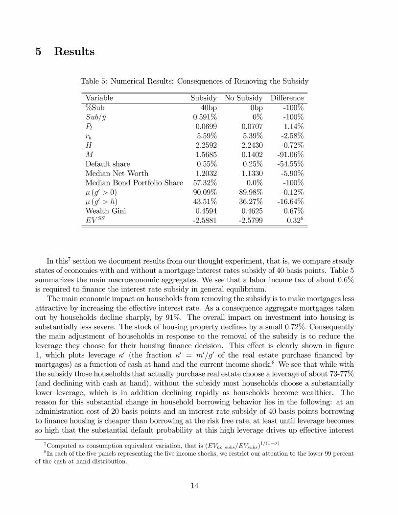
5 Results

Table 5: Numerical Results: Consequences of Removing the Subsidy

Variable Subsidy No Subsidy Difference%Sub 40bp 0bp -100%Sub/y 0.591% 0% -100%Pl 0.0699 0.0707 1.14%rb 5.59% 5.39% -2.58%H 2.2592 2.2430 -0.72%M 1.5685 0.1402 -91.06%Default share 0.55% 0.25% -54.55%Median Net Worth 1.2032 1.1330 -5.90%Median Bond Portfolio Share 57.32% 0.0% -100%μ (g0 > 0) 90.09% 89.98% -0.12%μ (g0 > h) 43.51% 36.27% -16.64%Wealth Gini 0.4594 0.4625 0.67%EV SS -2.5881 -2.5799 0.326

In this7 section we document results from our thought experiment, that is, we compare steadystates of economies with and without a mortgage interest rates subsidy of 40 basis points. Table 5summarizes the main macroeconomic aggregates. We see that a labor income tax of about 0.6%is required to finance the interest rate subsidy in general equilibrium.The main economic impact on households from removing the subsidy is to make mortgages less

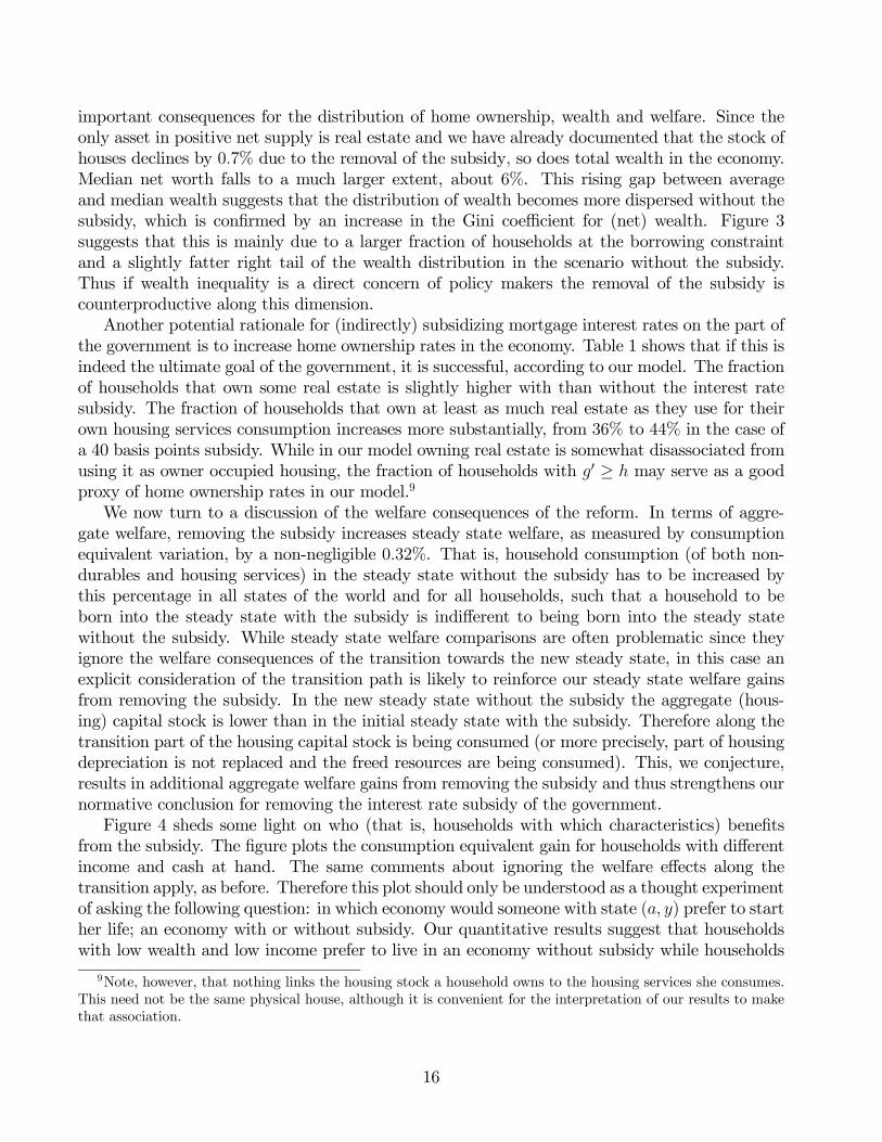
attractive by increasing the effective interest rate. As a consequence aggregate mortgages takenout by households decline sharply, by 91%. The overall impact on investment into housing issubstantially less severe. The stock of housing property declines by a small 0.72%. Consequentlythe main adjustment of households in response to the removal of the subsidy is to reduce theleverage they choose for their housing finance decision. This effect is clearly shown in figure1, which plots leverage κ0 (the fraction κ0 = m0/g0 of the real estate purchase financed bymortgages) as a function of cash at hand and the current income shock.8 We see that while withthe subsidy those households that actually purchase real estate choose a leverage of about 73-77%(and declining with cash at hand), without the subsidy most households choose a substantiallylower leverage, which is in addition declining rapidly as households become wealthier. Thereason for this substantial change in household borrowing behavior lies in the following: at anadministration cost of 20 basis points and an interest rate subsidy of 40 basis points borrowingto finance housing is cheaper than borrowing at the risk free rate, at least until leverage becomesso high that the substantial default probability at this high leverage drives up effective interest

7Computed as consumption equivalent variation, that is (EVno subs/EVsubs)1/(1−σ)

8In each of the five panels representing the five income shocks, we restrict our attention to the lower 99 percentof the cash at hand distribution.

14

rates. Note that since the asset that is being leveraged against, housing, is risky, so even ifhouseholds can borrow at rate lower than the risk free rate, there is no arbitrage opportunityfor them. Without the subsidy taking out mortgages comes at an interest premium of 20 basispoints over the risk-free lending rate because of the administrative costs for mortgages. Thusnot surprisingly the propensity of households to borrow against the house declines substantially,relative to the subsidy.Figure 2 plots the share of net worth a household holds in the risk-free asset (i.e. bonds),

rather than the risky asset (housing). Bond portfolio shares are increasing in a household’s cashat hand, which is especially pronounced with the subsidy. While this behavior of householdsmay sound counterintuitive at first (wealth-poorer households putting a larger share of theirwealth into the risky, rather than the safe asset), it is in line with recent work on portfolio choicebehavior (see Cocco et al. (2005) or Haliassos and Michaelides (2001)). These authors haveargued that it should be households with high cash at hand that hold a higher share of theirportfolio in the save asset. Households with high net worth tend to be people with high financialrelative to human wealth (the present discounted value of future labor income). As such, thesehouseholds expect to finance their current and future consumption primarily with capital income,whereas low cash-at-hand people tend to rely mostly on their labor income. Thus it is relativelymore important for the high cash at hand people not to be exposed to a lot of financial assetreturn risk. In fact, since idiosyncratic labor income shocks and house depreciation shocks areuncorrelated in our model, housing is a good asset for hedging labor income risk (of course thebond is even better in this regard, but has a lower expected return). In addition, bond portfolioshares are substantially lower without the subsidy that with the subsidy. This is plausible inlight of the fact that the real interest rate on the bond is lower without than with the subsidy,but the expected return on the risky asset, housing, rises because of the increase in the rentalrate of houses Pl. As a consequence of this general shift in households’ portfolio composition theshare of bonds in the median net worth households’ portfolio declines substantially; whereas thishousehold holds 57% of its net worth in bonds with the subsidy, this share drops to zero withoutthe subsidy.The behavioral changes induced by a change in the subsidy have significant general equi-

librium price effects. The reduction in the attractiveness of mortgages is also reflected in asubstantial decline in aggregate default rates which fall from 0.55% to 0.25% per year. Notethat since default and foreclosure is costly in terms of real resources, this reduction will be anontrivial factor in the welfare evaluation of the change of the government’s subsidy policy. Sincethe supply of housing declines because of the increase in its financing cost, the equilibrium rentalprice of housing increases, by slightly more than one percent. The equilibrium risk-free interestrate declines by 20 basis points in response to the removal of the subsidy since the demand forloans to finance house purchases collapses. Thus while the reduction of the subsidy increases theeffective interest rate on mortgages, holding leverage constant, by 40 basis points, half of thatincrease is offset by the general equilibrium effect on the interest rate that a reduction in thedemand for loans has. Furthermore, in the aggregate the reduction in the attractiveness of mort-gages is also reflected in a substantial decline in aggregate default rates which fall from 0.55% to0.25% per year. Note that since default and foreclosure is costly in terms of real resources, thisreduction will be a nontrivial factor in the welfare evaluation of the change of the government’ssubsidy policy.Given that the subsidy only benefits home owners one would expect that removing it has

15

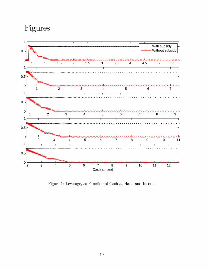
important consequences for the distribution of home ownership, wealth and welfare. Since theonly asset in positive net supply is real estate and we have already documented that the stock ofhouses declines by 0.7% due to the removal of the subsidy, so does total wealth in the economy.Median net worth falls to a much larger extent, about 6%. This rising gap between averageand median wealth suggests that the distribution of wealth becomes more dispersed without thesubsidy, which is confirmed by an increase in the Gini coefficient for (net) wealth. Figure 3suggests that this is mainly due to a larger fraction of households at the borrowing constraintand a slightly fatter right tail of the wealth distribution in the scenario without the subsidy.Thus if wealth inequality is a direct concern of policy makers the removal of the subsidy iscounterproductive along this dimension.Another potential rationale for (indirectly) subsidizing mortgage interest rates on the part of

the government is to increase home ownership rates in the economy. Table 1 shows that if this isindeed the ultimate goal of the government, it is successful, according to our model. The fractionof households that own some real estate is slightly higher with than without the interest ratesubsidy. The fraction of households that own at least as much real estate as they use for theirown housing services consumption increases more substantially, from 36% to 44% in the case ofa 40 basis points subsidy. While in our model owning real estate is somewhat disassociated fromusing it as owner occupied housing, the fraction of households with g0 ≥ h may serve as a goodproxy of home ownership rates in our model.9

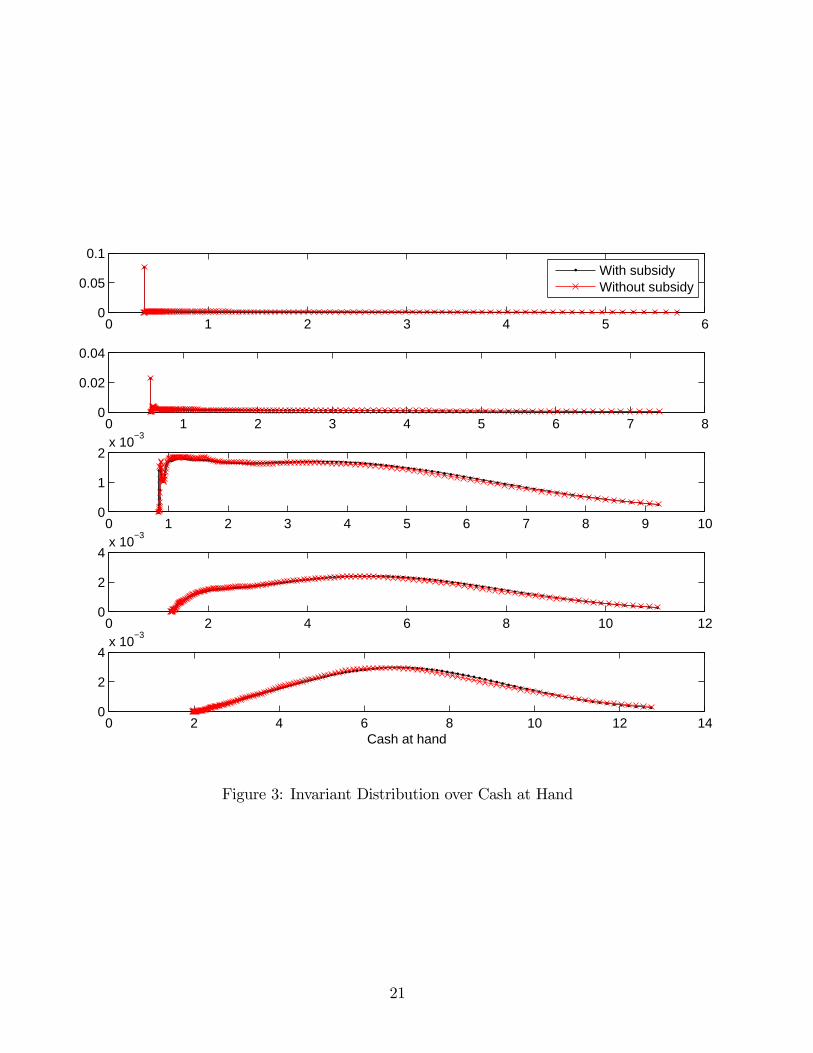
We now turn to a discussion of the welfare consequences of the reform. In terms of aggre-gate welfare, removing the subsidy increases steady state welfare, as measured by consumptionequivalent variation, by a non-negligible 0.32%. That is, household consumption (of both non-durables and housing services) in the steady state without the subsidy has to be increased bythis percentage in all states of the world and for all households, such that a household to beborn into the steady state with the subsidy is indifferent to being born into the steady statewithout the subsidy. While steady state welfare comparisons are often problematic since theyignore the welfare consequences of the transition towards the new steady state, in this case anexplicit consideration of the transition path is likely to reinforce our steady state welfare gainsfrom removing the subsidy. In the new steady state without the subsidy the aggregate (hous-ing) capital stock is lower than in the initial steady state with the subsidy. Therefore along thetransition part of the housing capital stock is being consumed (or more precisely, part of housingdepreciation is not replaced and the freed resources are being consumed). This, we conjecture,results in additional aggregate welfare gains from removing the subsidy and thus strengthens ournormative conclusion for removing the interest rate subsidy of the government.Figure 4 sheds some light on who (that is, households with which characteristics) benefits

from the subsidy. The figure plots the consumption equivalent gain for households with differentincome and cash at hand. The same comments about ignoring the welfare effects along thetransition apply, as before. Therefore this plot should only be understood as a thought experimentof asking the following question: in which economy would someone with state (a, y) prefer to starther life; an economy with or without subsidy. Our quantitative results suggest that householdswith low wealth and low income prefer to live in an economy without subsidy while households

9Note, however, that nothing links the housing stock a household owns to the housing services she consumes.This need not be the same physical house, although it is convenient for the interpretation of our results to makethat association.

16

with high current income y ∈ {y4, y5} and high wealth benefit from the subsidy. This is dueto mainly two reasons: first, the subsidy keeps interest rates on wealthy households’ assets high(because of the stronger mortgage demand), and second, it provides these households (whichinvest and leverage substantially in real estate) with a direct subsidy for this investment strategy.On the other hand, poorer households derive a larger share of their income from labor incomewhich is subject to the tax that finances the mortgage rate subsidy. Thus these householdsbenefit more strongly from removing the subsidy and the tax that comes with it, especially iftheir wealth falls into a region where debt-financed investment into real estate is suboptimal andthus the subsidy does not apply to these households.

6 Conclusions

We constructed a model with competitive housing and mortgage markets where the governmentprovides banks with insurance against an aggregate shock to their solvency. We used this modelto evaluate aggregate and distributional impacts of this implicit government subsidy to housing.Our main findings are that the subsidy policy leads to a higher housing stock and more mortgageswith higher leverage leading to more mortgage delinquencies. The subsidy mostly benefits highincome and mostly high wealth households. The aggregate welfare effect of the subsidy is negativedespite the higher aggregate holdings of the housing asset.

References

[1] Aiyagari, S. R. (1994): “Uninsured Idiosyncratic Risk and Aggregate Saving,” QuarterlyJournal of Economics, 109, 659—684.

[2] Attanasio, O. P. (1999). Consumption. In J. B. Taylor and M. Woodford Eds. Handbook ofMacroeconomics Vol. 11, Amsterdam, North-Holland.

[3] Bewley, T. F. (1986). Stationary Monetary Equilibrium with a Continuum of IndependentlyFluctuating Consumers. In W. Hildenbrand and A. Mas-Colell Eds. Contributions to Math-ematical Economics in Honor of Gerald Debreu, Amsterdam, North-Holland.

[4] Calhoun, Charles A., (1996): “OFHEO House Price Indexes: HPI Technical Description.”OFHEO paper.

[5] Congressional Budget Office (CBO) (2001): Federal Subsidies and the Housing GSEs, Wash-ington, D.C.: GPO.

[6] Chatterjee, S., D. Corbae, M. Nakajima and V. Rios-Rull (2005): “A Quantitative Theoryof Unsecured Consumer Credit with Risk of Default,”Working Paper 05-18, Federal ReserveBank of Philadelphia.

[7] Cocco, J., F. Gomes and P. Maenhout (2005): “Consumption and Portfolio Choice over theLife-Cycle,” Review of Financial Studies, 18(2), 491-533..

17

[8] Frame, Scott and Larry Wall (2002a): “Financing Housing through Government-SponsoredEnterprises” Economic Review, Federal Reserve Bank of Atlanta, First Quarter 2002.

[9] Frame, Scott and Larry Wall (2002b): “Fannie Mae’s and Freddie Mac’s Voluntary Initia-tives: Lessons from Banking”. Economic Review, Federal Reserve Bank of Atlanta, FirstQuarter 2002.

[10] Gervais, M. (2001): “Housing Taxation and Capital Accumulation,” Journal of MonetaryEconomics, 49, 1461-1489.

[11] Gruber, J. and R. Martin (2003): “Precautionary Savings and the Wealth Distribution witha Durable Good,” Interantional Finance Discussion Papers 773, Federal Reserve Board.

[12] Gourinchas, P. and J. A. Parker (2002). Consumption over the Life Cycle. Econometrica,Vol. 70, No. 1, pp. 47-89.

[13] Haliassos, M. and A. Michaelides (2003): “Portfolio Choice and Liquidity Constraints,”International Economic Review, 44, 143-78.

[14] Pennington-Cross, Anthony (2004): “The Value of Foreclosed Property: HousePrices, Foreclosure Laws, and Appraisals,” OFHEO Working Paper 04-1. Available athttp://www.ofheo.gov/media/pdf/workingpaper041.pdf

[15] Storesletten, K., C. Telmer, and A. Yaron (2004): “Consumption and Risk Sharing over theLife Cycle,” Journal of Monetary Economics, 51, 609—633.

[16] Tauchen, G. and R. Hussey (1991): “Quadrature-BasedMethods for Obtaining ApproximateSolutions to Nonlinear Asset Pricing Models,” Econometrica, Vol. 59, No. 2. (Mar., 1991),pp. 371-396.

18

Figures

0.5 1 1.5 2 2.5 3 3.5 4 4.5 5 5.50

0.5

1

1 2 3 4 5 6 70

0.5

1

1 2 3 4 5 6 7 8 90

0.5

1

2 3 4 5 6 7 8 9 10 110

0.5

1

2 3 4 5 6 7 8 9 10 11 120

0.5

1

Cash at hand

With subsidyWithout subsidy

Figure 1: Leverage, as Function of Cash at Hand and Income

19

0 1 2 3 4 5 60

0.5

1

0 1 2 3 4 5 6 7 80

0.5

1

0 1 2 3 4 5 6 7 8 9 100

0.5

1

0 2 4 6 8 10 120

0.5

1

0 2 4 6 8 10 12 140

0.5

1

Cash at hand

With subsidyWithout subsidy

Figure 2: Bond Portfolio Share as Function of Cash at Hand and Income

20

0 1 2 3 4 5 60

0.05

0.1

0 1 2 3 4 5 6 7 80

0.02

0.04

0 1 2 3 4 5 6 7 8 9 100

1

2x 10

−3

0 2 4 6 8 10 120

2

4x 10

−3

0 2 4 6 8 10 12 140

2

4x 10

−3

Cash at hand

With subsidyWithout subsidy

Figure 3: Invariant Distribution over Cash at Hand

21

0 1 2 3 4 5 60

0.005

0.01

0 1 2 3 4 5 6 7 80

0.005

0.01

0 1 2 3 4 5 6 7 8 9 10−0.01

0

0.01

0 2 4 6 8 10 12−0.01

0

0.01

0 2 4 6 8 10 12 14−5

0

5x 10

−3

Cash at hand

Figure 4: Steady State Welfare Consequences of Abolishing the Subsidy

22