Horizontally Explicit and Vertically Implicit (HEVI) Time DiscretizationScheme for a Discontinuous Galerkin Nonhydrostatic Model

LEI BAO

Department of Applied Mathematics, University of Colorado Boulder, Boulder, Colorado

ROBERT KLÖFKORN AND RAMACHANDRAN D. NAIR

National Center for Atmospheric Research,* Boulder, Colorado

(Manuscript received 25 March 2014, in final form 23 October 2014)

ABSTRACT

A two-dimensional nonhydrostatic (NH) atmospheric model based on the compressible Euler system has

been developed in the (x, z) Cartesian domain. The spatial discretization is based on a nodal discontinuous

Galerkin (DG) method with exact integration. The orography is handled by the terrain-following height-

based coordinate system. The time integration uses the horizontally explicit and vertically implicit (HEVI)

time-splitting scheme, which is introduced to address the stringent restriction on the explicit time step size due

to a high aspect ratio between the horizontal (x) and vertical (z) spatial discretization. The HEVI scheme is

generally based on the Strang-type operator-split approach, where the horizontally propagating waves in the

Euler system are solved explicitly while the vertically propagating waves are treated implicitly. As a conse-

quence, the HEVI scheme relaxes the maximum allowed time step to be mainly determined by the horizontal

grid spacing. The accuracy of the HEVI scheme is rigorously compared against that of the explicit strong

stability-preserving (SSP) Runge–Kutta (RK) scheme using several NH benchmark test cases. The HEVI

scheme shows a second-order temporal convergence, as expected. The results of the HEVI scheme are

qualitatively comparable to those of the SSP-RK3 scheme. Moreover, the HEVI DG formulation can also be

seamlessly extended to account for the second-order diffusion as in the case of the standard SSP-RK DG

formulation. In the presence of orography, theHEVI scheme produces high quality results, which are visually

identical to those produced by the SSP-RK3 scheme.

1. Introduction

With an increased amount of supercomputing resources

available to present-daymodelers, it is possible to develop

global atmosphericmodels with horizontal grid resolution

of the order of a few kilometers. At this fine resolution,

the models require a set of nonhydrostatic (NH) govern-

ing equations in order to resolve clouds at a global scale

(Tomita et al. 2008). However, this necessitates the de-

velopment of spatial and temporal discretization schemes

that are capable of facilitating excellent parallel efficiency

on peta-scale computers. Numerical schemes that can ad-

dress these challenges should have computationally desir-

able localproperties such as compact computational stencils,

high on-processor operations, and minimal communica-

tion footprints. There is a renewed interest in developing

newNHmodels based on finite-volume (FV; Ahmad and

Linedman 2007; Norman et al. 2011; Skamarock et al.

2012; Ullrich and Jablonowski 2012; Li et al. 2013) and

Galerkin methods (Giraldo and Restelli 2008; Giraldo

et al. 2013; Brdar et al. 2013), which are designed to ad-

dress these computational challenges to a great extent.

Among the emerging approaches for spatial discretiza-

tion, the discontinuous Galerkin (DG) method stands out

as a strong candidate, owing to its several computationally

attractive features such as local and global conservation,

high-order accuracy, high parallel efficiency, and geo-

metric flexibility. The DG method may be viewed as

a hybrid approach combining the desirable features of

two standard numerical discretization approaches: FV

*The National Center for Atmospheric Research is sponsored

by the National Science Foundation.

Corresponding author address: R. D. Nair, Computational and

Information System Laboratory, National Center for Atmospheric

Research, Boulder, CO 80305.

E-mail: rnair@ucar.edu

972 MONTHLY WEATHER REV IEW VOLUME 143

DOI: 10.1175/MWR-D-14-00083.1

� 2015 American Meteorological Society

and the finite-element (spectral element) methods. The

DG spatial discretization combined with Runge–Kutta

(RK) time integration provides a class of robust algo-

rithms known as the RKDG method for solving con-

servation laws (Cockburn 1997). The application of DG

methods in atmospheric modeling is becoming in-

creasingly popular in both hydrostatic (Nair et al. 2009)

and NH modeling (Giraldo and Restelli 2008; Brdar

et al. 2013). A recent review by Nair et al. (2011) pres-

ents various DG applications in atmospheric science

with an extensive list of references. By virtue of the

aforementioned advantages, we employ a DG method

for the spatial discretization for a NH model based on

the compressible Euler system in two dimensions (2D)

on the x–z plane, under the terrain-following height-

based coordinate system (Gal-Chen and Sommerville

1975); hereafter this is referred to as the DG-NHmodel.

The advantage of explicit time-stepping schemes is

their simplicity and high parallel efficiency, namely, the

minimal interprocessor communication, when evaluat-

ing the equations of motion (see, e.g., Dennis et al.

2012). Explicit strong stability-preserving (SSP)-RK

time integration is typically used together with Pk-DG

methods, which employ a set of polynomials of degree

up to k, but results in a severe Courant–Friedrichs–Lewy

(CFL) stability limit of 1/(2k 1 1); note that this re-

lationship is approximate for k . 1 [see Cockburn

(1997)]. The penalizing drawback of this combination is

that a numerical method that is high order in space re-

quires a smaller time step size than the corresponding

low-order variant with the same grid spacing. Besides,

for the compressible NH system, the physically in-

significant fast-moving sound waves dictate the explicit

time step size, which imposes a stringent stability con-

straint on the whole system and impedes the computa-

tional efficiency. To make matters worse, the vertical

grid spacing is several magnitudes smaller than the

horizontal grid spacing (’1:1000) in a typical global

atmospheric model. The vertical discretization with

small grid spacing permits only a tiny explicit time step

size, and atmospheric models based on this option have

only a limited practical value. There are established

models based on the anelastic or soundproof system of

equations, which eliminates sound waves from the con-

tinuous system (Prusa et al. 2008). Nevertheless, the

solution process of such models involves expensive el-

liptic solvers, and the ultimate efficiency of the model is

tied up with that of the elliptic solvers and associated

preconditioners. A fully implicit time-stepping ap-

proach might be devised to solve the compressible NH

model (St-Cyr andNeckels 2009), but this again requires

expensive implicit solvers. In general, the cost effec-

tiveness (parallel efficiency) of models that rely upon

global elliptic solvers, is not clear in a peta-scale com-

puting environment.

The split-explicit and semi-implicit time stepping

schemes are two possible alternatives that are widely used

in many operational weather forecasting centers. Split-

explicit methods fall into the subcycling category, where

the shorter substeps are used for the faster-moving

acoustic and gravity terms of the governing equations

(Tomita et al. 2008). In semi-implicit models, acoustic and

gravity waves are usually treated implicitly while the ad-

vection parts are solved explicitly (Durran 1999; Simarro

et al. 2013). Consequently, the time step size is relaxed

from the speed of sound and the gravity waves, which

shows relatively better efficiency at the cost of a Helm-

holtz solver. Implicit–explicit (IMEX) schemes, a variant

of semi-implicit schemes, treat the fast time-scale terms

implicitly and the slow time-scale terms explicitly. Restelli

and Giraldo (2009) studied IMEX time integrators used

with the DG spatial discretization to improve the effi-

ciency of the scheme by rewriting the problem in the form

of a pseudo-Helmholtz operator.

The horizontal explicit and vertical implicit (HEVI)

schemes are another type of splitting approach in which

the terms responsible for the horizontal dynamics are

solved explicitly while treating the vertical terms im-

plicitly (Satoh 2002). Note that the HEVI scheme may

be viewed as a framework where the IMEX time in-

tegration schemes can be incorporated. In a recent work,

Weller et al. (2013) give a detailed comparison of pop-

ular options of HEVI time stepping schemes. For HEVI

scheme the maximum time step size is only limited by

the horizontal grid spacing and, this choice of time step

is usually acceptable in the real application as shown in

Skamarock and Klemp (2008) and Tomita et al. (2008).

A linear analysis of various RK HEVI schemes can be

found in Lock et al. (2014). Recently, there is a renewed

interest on the applications of the HEVI schemes for

high-order methods as used in NH modeling. Ullrich

and Jablonowski (2012) examined three RK IMEX

schemes for HEVI splitting of nonhydrostatic solutions

using a FV spatial discretization, which includes the crude-

splitting, Strang-carryover splitting and (Ascher–Ruuth–

Spiteri) ARS(2, 3, 3) of Ascher et al. (1997). A novelty of

Ullrich and Jablonowski (2012) is the recycling of the

solution of the previous time step as the solution for the

first implicit solution for the Strang-carryover scheme.

The computational expense due to the implicit solver is

optimized by using a Rosenbrock-type solver, which is

essentially one Newton iteration. Giraldo et al. (2013)

studied the accuracy and efficiency of IMEX methods,

when discretized with continuous Galerkin methods, in

semi-implicit andHEVI form for nonhydrostatic 3Dflows

(both on the globe and in the limited area).

MARCH 2015 BAO ET AL . 973

In the present work, we investigate the performance

of HEVI time-stepping method with the DG-NHmodel

(hereafter referred to as HEVI-DG) using an operator-

split approach. We also use the explicit SSP-RKmethod

without time splitting for the DG-NH model to provide

results for comparison. To extend the time step size with

explicit RKmethods, we employmoderate orderPk-DG

where k# 4, with exact integration usingGauss–Legendre

quadratures, which is different from the high-order

formulation considered in Giraldo and Restelli (2008).

The parallel version of the model is implemented with

a horizontal domain decomposition that assumes that

the vertical column (z direction) of data is not distrib-

uted across the processors. In this way, the vertical implicit

solver does not need any interprocessor communication.

Furthermore, we can take advantage of the existing

knowledge of the IMEX-RK schemes to generateHEVI-

DG schemes with the desired properties and temporal

accuracy.

Theorganizationof thepaper is as follows. The governing

equations and the computational forms are described

in section 2. The DG spatial discretization is discussed in

section 3, followed by the time integration schemes in

section 4. The numerical results for several benchmark test

cases are presented in section 5. Conclusions and some fu-

turework are described in section 6. The implementation of

the diffusion process is detailed in the appendix.

2. The idealized nonhydrostatic model

The model is designed to simulate two-dimensional

(2D) airflow over a (x, z) Cartesian domain. The com-

pressible nonhydrostatic Euler system of equations can

be written in the following vector form, without speci-

fying the coordinate system:

›r

›t1$ � (ru)5 0, (1)

›ru

›t1$ � (ru5u1 pI)52rgk, and (2)

›ru

›t1$ � (ruu)5 0, (3)

where r is the air density, 5 is the tensor (outer)

product, k is the basis vector in the z direction with unit

length, u5 (u,w)T is the velocity vector with the vertical

component w 5 u � k, p is the pressure, g is the accel-

eration due to gravity, I represents the 2 3 2 identity

matrix, and $ � is the divergence operator. The potentialtemperature u is related to the real temperature T by

u5T( p0/p)Rd/cp . The above system is closed by the

equation of state, p 5 C0(ru)g, where C0 5Rg

dp2Rd/cy0 .

The reference surface pressure p0 5 105 Pa, and the

other thermodynamic constants are given by g 5 cp/cy,

Rd 5 287 J kg21K21, cp 5 1004 J kg21K21, and cy 5717 J kg21K21.

a. Terrain-following height-based coordinate

Accurate representation of terrain is very important

for practical NH modeling where mountain lee waves

are forced by the irregularities (topography) of the

earth’s surface. The height-based vertical coordinate is

popular in many nonhydrostatic global models (Prusa

et al. 2008; Tomita et al. 2008; Skamarock et al. 2012).

The terrain-following height-based coordinate offers

more flexibility and accuracy compared to pressure-

based coordinates, and is free from time-dependent

terrain metrics (Toy and Randall 2009). Although the

DG method is capable of handling complex domain

(Giraldo and Restelli 2008), we prefer to use the clas-

sical terrain-following height coordinates introduced by

Gal-Chen and Sommerville (1975). Recently, more so-

phisticated terrain-following coordinate systems were

developed (Schär et al. 2002; Klemp 2011) and will be

considered for future development.

If h5 h(x) is the prescribed mountain profile and zT is

the top of the model domain, then the vertical z height

coordinate can be transformed to the monotonic z co-

ordinate using the following mapping:

z5zTz2h(x)

zT2h(x), z(z)5h(x)1z

zT2h(x)

zT; h(x)#z#zT .

(4)

This coordinate transformation invariably introduces

tensor quantities and metric terms associated with map-

ping as described in Gal-Chen and Sommerville (1975),

Clark (1977), and Satoh (2002). Following the standard

notations (Satoh 2002), the Jacobian of the trans-

formation is given byffiffiffiffiffiG

pand defined as

ffiffiffiffiffiG

p5

�›z

›z

�x5const

, G13 5

�›z

›x

�z5const

, (5)

where the Jacobian and the metric term G13 are in-

dependent of time. For an arbitrary scalar c, we have the

following relation connecting (x, z) and (x, z) coordinate

systems (Clark 1977),

ffiffiffiffiffiG

p ›c

›z5

›c

›z, (6)

ffiffiffiffiffiG

p �›c

›x

�z5const

5

�›

›x(ffiffiffiffiffiG

pc)

����z5const

1›

›z(ffiffiffiffiffiG

pG13c)

�.

(7)

974 MONTHLY WEATHER REV IEW VOLUME 143

The vertical velocity in the transformed system (x, z) is ~w

and defined as

~w5dz

dt5

1ffiffiffiffiffiG

p (w1ffiffiffiffiffiG

pG13u) . (8)

The divergence operation for a vector field F 5 (Fx, Fz)

under the coordinate transformation takes the following

form:

$ � F51ffiffiffiffiffiG

p�›

›x(ffiffiffiffiffiG

pFx)1

›

›z(Fz1

ffiffiffiffiffiG

pG13Fx)

�. (9)

b. Removal of the hydrostatic balanced state

In the context of atmospheric modeling, it is common

to write the thermodynamic variables as the sum of the

mean state (reference state) (�) and perturbation (�)0(Skamarock and Klemp 2008):

r(x, z, t)5 r(z)1 r0(x, z, t) , (10)

u(x, z, t)5 u(z)1 u0(x, z, t) , (11)

p(x, z, t)5 p(z)1 p0(x, z, t), and (12)

(ru)(x, z, t)5 ru(z)1 (ru)0(x, z, t) , (13)

where the mean state satisfies the hydrostatic balance:

dp

dz52rg . (14)

Themean-state part of the thermodynamic variables is in

hydrostatic balance and makes no contribution to drive the

dynamics. In contrast, the dynamic processes, or the ac-

celerations, are triggered and influenced by the perturba-

tion part (Clark 1977). Besides, the deviations due to the

nonhydrostatic effect from the hydrostatic balance are rel-

atively small, except for certain extreme cases such as tor-

nadoes. Embodying the mean state in the whole system

may introduce some errors in approximating the hydro-

static equilibrium numerically, which may generate some

spurious verticalmomentum.Therefore, the hydrostatically

balanced mean state is removed from the Euler system.

c. Governing equations

Combining the relations (5)–(9) and substituting in

the Euler system (1)–(3) results in the following general

2D Euler system in the transformed (x, z) coordinates:

›U

›t1

›Fx(U)

›x1›Fz(U)

›z5 S(U)

0›U

›t1$ � F(U)5S(U) , (15)

where U is the state vector and U5 [ffiffiffiffiffiG

pr0,

ffiffiffiffiffiG

pru,ffiffiffiffiffi

Gp

rw,ffiffiffiffiffiG

p(ru)0]T, S is the source term, and S5

[0, 0,2ffiffiffiffiffiG

pr0g, 0]T. The variables Fx and Fz are the flux

vectors along x and z directions, respectively, which

have the following forms:

Fx5

2666664

ffiffiffiffiffiG

pruffiffiffiffiffi

Gp

(ru2 1p0)ffiffiffiffiffiG

pruwffiffiffiffiffi

Gp

ruu

3777775, Fz 5

266664

r ~w

ru ~w1ffiffiffiffiffiG

pG13p0

rw ~w1 p0

r ~wu

377775,

S5

266664

0

0

2ffiffiffiffiffiG

pr0g

0

377775 ,

(16)

and F 5 (Fx, Fz). The compressible 2D Euler system in

(15) is the basis for the DG-NH model. Note that in the

absence of topography [h(x) 5 0, z 5 z], we haveffiffiffiffiffiG

p5 1, G13 5 0 and w5 ~w.

3. DG spatial discretization

The DGmethod is usually termed as a hybrid scheme,

combining the best properties of the spectral element

and FV methods. The application of DGmethods in the

atmospheric community is a vigorous research field [see

Nair et al. (2011) for details], and we only provide a brief

outline of theDG discretization process herein.Without

loss of generality, we consider a scalar component of the

Euler system in (15) without orography on a rectangular

Cartesian domain D for DG spatial discretization:

›U

›t1$ � F(U)5S(U), in (0, tT ]3D; " (x, z) 2 D,

(17)

where U 5 U(x, z, t), F is the flux function, and S is the

source term; tT is the prescribed time. Initially, u0(x, z)5u(x, z, t 5 0) and suitable boundary conditions are

imposed.

The DG spatial discretization procedure consists of

partitioning the domainD into nonoverlappingNx 3Nz

regular elements Vij, such that

Vij 5 [xi21/ 2, xi11/ 2]5[zj21/2, zj11/2] ,

i5 1, . . . , Nx, j5 1, . . . , Nz and seeking an approximate

solution Uh for U on each element, which satisfies that

Uh 2 Vkh5 [u 2 L2(D):ujV

i, j2 Pk(Vi,j), " Vi,j 2 D] ,

MARCH 2015 BAO ET AL . 975

where Pk 5 spanfxmzn: 0#m, n# kg. The aforemen-

tioned process is identical on each element, so we con-

sider a generic element Ve herein.

a. Weak Galerkin formulation

Multiplying (17) by a test function uh 2 Vkh and in-

tegrating by parts over Ve leads to the following weak

Galerkin formulation:

›

›t

ðV

e

Uhuh dV2

ðV

e

F(Uh) � $uh dV1

ðGe

F̂(Uh) � nuh dG

5

ðV

e

S(Uh)uh dV ,

(18)

where n is the outward-facing unit normal vector of the

edge Ge, and F̂(Uh) is the numerical flux, which is crucial

to resolve the discontinuity of the interelement solu-

tions. In general, high-order DG schemes employing

polynomials of degree up to k are often referred to as

Pk-DG methods.

In (18), for simplicity and efficiency, the numerical

flux is chosen as Lax–Friedrichs flux (Cockburn 1997):

F̂(U1h ,U2

h )51

2f[F(U2

h )1F(U1h )] � n2lmax(U

1h 2U2

h )g,(19)

where U2h and U1

h are the left and right limits, re-

spectively, of the solution at the interface Ge. For the

Euler system, lmax is the upper bound on the absolute

value of eigenvalues of the flux Jacobian F0(U), which is

a function of the wind speed u and speed of sound waves

c, evaluated at the interface:

lmax5maxfjy2j1 c, jy1j1 cg, c5ffiffiffiffiffiffiffiffiffiffiffiffiffigRdT

q,

y6 5 u6 � n . (20)

b. Nodal basis functions

The integral equation (18) plays a central role in the

DG discretization. The accuracy and efficiency of the

scheme are greatly dependent on the particular choice

for Vkh and the quadrature rules chosen for the surface

and line integrals.

In the current study, we are focusing only onmoderate

order Pk-DG discretization for the DG-NH model with

k# 4. Note that a major limitation of the DG scheme is

the stringent CFL stability constraint associated with the

explicit time stepping. Reducing the order of accuracy

significantly improves the CFL stability restriction with

explicit time stepping and, therefore, allows for imple-

mentation of limiting (positivity preserving) algorithms,

based on those designed for FV methods (Zhang and Nair

2012).

To solve the weak form (18), we introduce an affine

mapping fromeachVe to a reference elementVQ5 [21, 1]2,

which simplifies the integrals in (18):

j52(x2 xi)

Dxi, Dxi 5 (xi11/2 2 xi21/ 2), and (21)

h52(z2 zj)

Dzj, Dzj 5 (zj11/2 2 zj21/2) , (22)

where (j, h) 2 VQ are local independent variables, and

xi 5 (xi11/2 1 xi21/2)/2 and zj 5 (zj11/2 1 zj21/2)/2.

For the computational efficiency, the nodal DG dis-

cretization is employed in the present work. The Lagrange

polynomials fhl(j)gkl50 are adopted as the basis functions,

the roots of which are a set of the chosenGauss quadrature

points (Karniadakis and Sherwin 2005), and they satisfy

the discrete orthogonal properties:

hl(jm)5 dlm, and

ð121

hl(j)hm(j) dj ’ wldlm ,

where wl are the weights associated with the quadrature

rule and dlm is the Kronecker function (dlm 5 0 if l 6¼m,

dlm 5 1 if l 5 m).

There are a range of choices for the quadrature rules,

among which Gauss–Legrendre (GL) and Gauss–

Lobatto–Legrendre (GLL) quadrature rules are the

most popular (Nair et al. 2011). ForPk-DGmethods, the

GL quadrature rule provides the exact integration of

(18), which is suitable for a moderate order (pk, k5 2, 3,

4) of approximation. The GL grid is chosen for the

present development. A schematic plot of the grids with

33 3 and 43 4GL quadrature points is shown in Fig. 1.

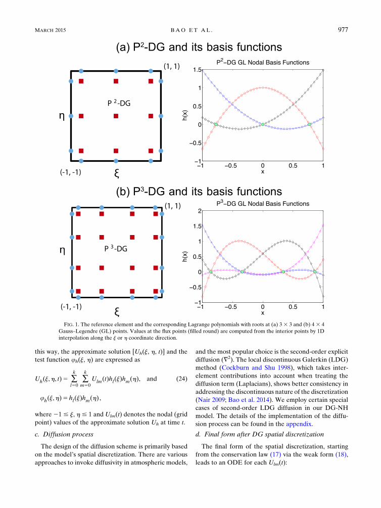
For the GL grid with the quadrature points fjmgkm50, the

Lagrange polynomial fhl(j)gkl50 and the corresponding

weight are given as

hl(j)jGL5Pk11(j)

P 0k11(jl)(j2 jl)

,

wljGL52

(12 j2l )[P0k11(jl)]

2, (23)

where Pk(j) is the kth degree Legendre polynomial and

P0k(j) is its derivative. Figure 1 shows these polynomials

for k 5 2, 3.

For 2D problems, as in the case of the DG-NHmodel,

we use a tensor product of the basis functions, which is

the basis set fhl(j)hm(h)g, where l, m 5 0, 1, . . . , k. In

976 MONTHLY WEATHER REV IEW VOLUME 143

this way, the approximate solution [Uh(j, h, t)] and the

test function uh(j, h) are expressed as

Uh(j,h, t)5 �k

l50�k

m50

Ulm(t)hl(j)hm(h), and (24)

uh(j,h)5 hl(j)hm(h) ,

where21# j, h# 1 and Ulm(t) denotes the nodal (grid

point) values of the approximate solution Uh at time t.

c. Diffusion process

The design of the diffusion scheme is primarily based

on the model’s spatial discretization. There are various

approaches to invoke diffusivity in atmospheric models,

and the most popular choice is the second-order explicit

diffusion (=2). The local discontinuous Galerkin (LDG)

method (Cockburn and Shu 1998), which takes inter-

element contributions into account when treating the

diffusion term (Laplacians), shows better consistency in

addressing the discontinuous nature of the discretization

(Nair 2009; Bao et al. 2014). We employ certain special

cases of second-order LDG diffusion in our DG-NH

model. The details of the implementation of the diffu-

sion process can be found in the appendix.

d. Final form after DG spatial discretization

The final form of the spatial discretization, starting

from the conservation law (17) via the weak form (18),

leads to an ODE for each Ulm(t):

FIG. 1. The reference element and the corresponding Lagrange polynomials with roots at (a) 3 3 3 and (b) 4 3 4

Gauss–Legendre (GL) points. Values at the flux points (filled round) are computed from the interior points by 1D

interpolation along the j or h coordinate direction.

MARCH 2015 BAO ET AL . 977

d

dtUlm(t)5

4

DxiDzjwiwj

[IGrad 1 IFlux1 ISource] , (25)

where the coefficients 4/(DxiDzjwiwj) constitute the in-

verted mass matrix for an element Vij. The term IFlux is

the line integral and, IGrad and ISource are the surface

integrals corresponding to the discretization of the weak

form in (18). Explicit definitions of these terms are given

in Nair et al. (2011). Therefore, the ODE in time cor-

responding to the scalar conservation law (17) is

d

dtUh(t)5L(Uh) , (26)

and for system (15) is

d

dtUh(t)5L(Uh) , (27)

where L (or L) indicates the spatial DG discretization.

4. Time integration procedure

In the construction of high-order RKDG methods

(hereafter, we use DG for RK-DG), the spatial terms

are discretized first, and the resulting ODE system for

the prognostic variables is solved by a proper time in-

tegration scheme. The DG spatial discretization of the

Euler system is fairly standard, which is elaborated on in

section 3; however, the design of an efficient time in-

tegrator is of predominant importance, especially when

we reach the nonhydrostatic scale.

We discuss the time integrator for an ODE system in

the following general form:

U0(t)5 f [U(t), t] in (0, tT ] , (28)

whereU(t) are the coefficients to the DG solutionUh(t)

in (24). For the Euler’s system in (27), the right-hand

side function f is given by

f [U(t), t]5L[Uh(t)] . (29)

In this paper, we investigate a HEVI-type splitting

approach and compare it with commonly used explicit

time stepping methods. All the time integrators con-

sidered in our development may be characterized as

RK-type methods.

a. RK methods

Given the solution Un at time tn, we use an s-stage RK

method toobtain the solution at the next time level t n11. For

a givenUn and some integer s. 0, the coefficientsA 2 Rs3s,

b 2 Rs, and c 2 R

s define the s-stage RK method:

Ki 5 f

tn 1 ciDt,U

n 1Dt �2

j51

AijKj

!, i5 1, . . . , s,

Un115Un1Dt �s

i51

biKi . (30)

The coefficients A5 [Aij], b5 [bi], and c5 [cj] form the

so-called Butcher tableau (Butcher 1987):

c A

bT.

For an explicit RK method, Aij 5 0 for all j $ i, which

corresponds to all entries of A on and above the diagonal

being zero. Some popular examples of explicit SSP-RK

methods (Gottlieb et al. 2001), which are widely used with

the DG discretization (Nair et al. 2011), are as follows:

d Heun’s method (SSP-RK2)

(two-stage second order)

0 0

1 1 0

1

2

1

2

.

d Explicit Runge–Kutta (SSP-RK3)

(three-stage third order)

0 0

1 1 0

1

2

1

4

1

40

1

6

1

6

2

3

.

For implicit RK methods, we consider diagonally im-

plicit RK (DIRK; Alexander 1977) methods. DIRK

methods are characterized by the fact that the coefficients

Aij 5 0 for j . i, in which case, all entries of A above the

diagonal are zero. DIRK methods have the advantage

that the resulting nonlinear systems can be solved one by

one. A popular DIRKmethod is given below (Alexander

1977):

d Crank–Nicholson (DIRK2)

(one-stage second order)

1

2

1

2

1

.

978 MONTHLY WEATHER REV IEW VOLUME 143

For the solution of the nonlinear system for each RK

stage, which arises due to the nonzero diagonal entries ofA

in (30), we apply a Jacobian-free Newton–Krylov (JFNK)

method (Knoll and Keyes 2004). A generalized minimal

residual (GMRES) (Saad and Schultz 1986) solver is ap-

plied for the linear system in each Newton step and the

application of the right-hand-side operator f in each

GMRES iteration is accomplished in amatrix-free fashion.

Explicit time integrators are relatively easy to imple-

ment and usually possess excellent parallel scalability.

However, the general drawback with the application of

explicit SSP-RK methods in DG methods is the severe

time step restrictions (i.e., a CFL number much smaller

than 1 has to be used). For the Pk-DG algorithm,

a heuristic estimation of the CFL number is given by

Cockburn (1997):

CDt

h,

1

2k1 1, (31)

where h 5 minfDx, Dzg, where Dz denotes the grid

spacing in vertical direction and Dx the grid spacing in

horizontal direction, and C 5 maxfjuj 1 c, jwj 1 cg,c5

ffiffiffiffiffiffiffiffiffiffiffiffigRdT

pis the speed of sound. The resulting time

step size for an explicit time integration scheme is usu-

ally very tiny. In contrast, the implicit ODE solver has

a large stability region, which admits a large time step

size, but is expensive to solve in general. The construc-

tion of the implicit solver formultidimensional problems

is usually complicated and requires complex nonlinear

solvers. The overall efficiency may not be competitive

with the explicit solver and the computational scalability

may even be degraded if the nonlinear solver is not

designed properly. The hope of an efficient time in-

tegrator, which enables a large time step size and ex-

cellent computational efficiency, has triggered a vast

research effort into implicit and semi-implicit time in-

tegration methods.

b. Horizontally explicit and vertically implicit(HEVI) scheme via Strang splitting

Apopular approach in atmospheric applications is the

HEVI approach. This is justified by the relatively large

difference of scales in the horizontal and vertical di-

rections (i.e., Dz� Dx). Although a large Dx still resultsin an acceptable CFL restriction for the present study,

the small Dz introduces noticeable difficulties due to the

severe CFL restriction in the vertical direction. As a re-

sult, a splitting approach with an implicit treatment in

the vertical direction stands out as a suitable alternative.

The horizontal direction is still treated explicitly, al-

lowing the usage of the excellent scaling behavior of

explicit methods. For the practical atmospheric appli-

cations, the horizontal CFL condition can be further

relaxed by subcycling or multirate integrations (Tomita

et al. 2008), which is beyond the scope of the present work.

In our development, the domain decomposition for

parallel computations is carried out in the horizontal

direction only, which is broadly embraced in the atmo-

spheric community (Michalakes et al. 2007). Therefore,

all data is locally accessible in the vertical direction and

an implicit treatment in the vertical direction does not

require any communication. As a consequence, we ex-

pect the excellent scaling performance on today’s many

core systems to be maintained.

We split the DG spatial operator L in (27) into

a horizontal (x) and a vertical (z) part such that

L(Uh)5Lx(Uh)1Lz(Uh) , (32)

where Lx and Lz are the DG 1D discretization to (33)

and (34), respectively:

›Uh

›t52

›Fx(Uh)

›x1 Sx, and (33)

›Uh

›t52

›Fz(Uh)

›z1 Sz . (34)

Note that, for thedimensional splitting usedhere, the source

term is decomposed asSx5 0 and Sz5 S. The definitions of

Fx, Fz, and S are given in (16). Instead of solving the full

system (28), we solve the system in the horizontal direction

(33) and the system in the vertical direction (34) separately

in a sequence, via the Strang-type splitting (Strang 1968).

Strang-type splitting has been successfully applied in FV

methods (Norman et al. 2011; Ullrich and Jablonowski

2012) and it also shows promising performances when ap-

plied to semi-Lagrangian DG methods for different geom-

etries by Guo et al. (2014). Given a time interval of size Dtand the solutionUn

h at tn, the corresponding Strang-splitting

scheme has the following steps:

U05Unh , (35)

d

dtU15Lx(U1) in (tn, tn1Dt/2],

U1(tn)5U0 , (36)

d

dtU2 5Lz(U2) in (tn, tn11],

U2(tn)5U1(t

n 1Dt/2) , (37)

d

dtU3 5Lx(U3) in (tn1Dt/2, tn11],

U3(tn 1Dt/2)5U2(t

n11), and (38)

Un11h 5U3(t

n11) . (39)

MARCH 2015 BAO ET AL . 979

This approach requires the solution of the three equa-

tions, (36)–(38), which means that the horizontal part is

solved for twice and the vertical part once (H-V-H). It

would also be possible to solve the system in V-H-V form,

but ideally the more expensive system should only be

solved once. In our choice, we only solve the vertical system

once. We also tested the Strang-carryover scheme (Ullrich

and Jablonowski 2012),which is essentiallyV-H-V,with the

first stage in the vertical is recycled from the previous

time step; however, the solution is found to be degraded,

even for a smooth test case.

Since we usually prefer higher order in the DG spatial

discretization, the time integrator will be the dominant

factor in the numerical error. Strang-type splitting permits

second-order temporal accuracy (Toro 1999), therefore,

we choose SSP-RK3 as the explicit time integrator for the

horizontal direction (33) and we solve the vertical di-

rection (34) either with the explicit RKmethod SSP-RK2,

which leads to an horizontal explicit and vertical explicit

(HEVE) method, for comparison studies, or with an im-

plicit time stepping method DIRK2, which is our HEVI

scheme. Therefore, the time integration schemes studied

in the present paper are given as follows:

HEVI (or HEVE) time integrator

1) Solve (36) via SSP-RK3,

2) Solve (37) via DIRK2 (or SSP-RK2), and

3) Solve (38) via SSP-RK3.

The introduction of the HEVE time integration

scheme is solely for the purpose of validating the idea of

dimensional splitting for DG methods and, in practice,

we would adopt the HEVI scheme for practical appli-

cations. When using an implicit method for the vertical

direction (34), it is observed that the CFL condition for

the whole system may be relaxed to the CFL condition

for the horizontal part only. In other words, Dt for theStrang-splitting can be chosen as the largest possible Dtof (33). In this way, the overall performance can be greatly

accelerated. Nevertheless, the necessity of solving an im-

plicit system introduces an additional overhead. In terms

of the performance of the DIRK methods, usually the

number of Newton iterations is very small (i.e., 1 or 2 and

usually not higher than 5). Therefore, the performance of

the implicit solver is closely related to the number of it-

erations of the linear solver. This can be reduced by proper

preconditioning. However, in the current implementation,

no preconditioning is applied. The construction of a proper

preconditioning method is ongoing work. In addition, be-

cause of our domain decomposition, we obtain an implicit

system for each vertical column,which is decoupled for the

other column systems. Therefore, no communication is

needed for the implicit solvers. Even a direct solver could

be applied since the system for one column is not that

large. This will overcome the need for preconditioning

the iterative solvers used otherwise.

The existing IMEXschemes (Ascher et al. 1997;Giraldo

et al. 2013) can be easily incorporated into the HEVI-DG

framework, which may yield some beneficial properties.

To apply an IMEX time integrator, we first rewrite our

problem such that we distinguish between a part that

should be treated implicitly, here Lim, and a part that

should be treated explicitly, here Lex, such that

d

dtUh 5Lim(Uh)1Lex(Uh) in (tn, tn11] . (40)

For the IMEX RK method, we define f im[U(t), t] 5Lim[U(t)] and f ex[U(t), t]5 Lex[U(t)]. The performance

of IMEX schemes combined with DG spatial dis-

cretization may be revisited in a future study.

5. Numerical experiments

To demonstrate and evaluate theHEVI time integration

scheme in the DG-NHmodel, we choose several standard

benchmark tests from the literature. Before detailing with

each test case, we briefly discuss some common features

such as the grid resolution, boundary conditions, and the

initialization process used in the DG-NH model.

a. Numerical experiments setup

The spatial resolution should take account of the grid

spacing within each element for the nodal DG (RK-DG)

method. For the GL case, the edge points of each ele-

ment are not included as solution points (see Fig. 1);

therefore, we use an approximate procedure to define

the minimum grid spacing for the Pk-DGmethod, which

has k 1 1 degrees of freedom (dof) in each direction.

The average grid spacing is defined in terms of dof as

Dx5Dxi/(k1 1), Dz5Dzj/(k1 1), (41)

where Dxi and Dzj are the element width in the x di-

rection and z direction, respectively [(21) and (22)]. We

employ uniform elements over the whole domain, and

use this convention in (41) as the grid resolution in our

DG-NH model. Note that our definition of grid spacing

is similar to Brdar et al. (2013) but different from that of

Giraldo andRestelli (2008), where they use theGLLgrid.

The DG-NH model, designed for a rectangular domain,

requires suitable boundary conditions for various test

cases. These include no-flux, periodic, and nonreflecting

type boundary specifications.

1) NO-FLUX BOUNDARY CONDITIONS

Essentially, the no-flux (or reflecting) boundary con-

ditions eliminate the normal velocity component to the

980 MONTHLY WEATHER REV IEW VOLUME 143

boundary and only keep the tangential component. For

an arbitrary velocity vector v, the no-flux boundary

condition results in v � n 5 0, where n is the outdrawn

normal vector from the boundary. We denote (yk, y?) asthe parallel (tangential) and perpendicular (normal)

components, respectively, of v along the boundary wall;

let the left and right values at the element edge of v

along the boundary be yL and yR, respectively. Then the

no-flux boundary conditions can be written in the fol-

lowing form:

y?R 52y?L , ykR 5 y

kL . (42)

The same idea is used for the flux vectors along the

boundary.

2) NONREFLECTING BOUNDARY CONDITIONS

The nonreflecting (or transparent) boundary condi-

tions are used to prevent the reflected waves from

reentering the domain, which may interfere or pollute

the flow structure. For the mountain test cases, non-

reflecting boundary conditions are commonly imposed

at the top (zT) and the lateral boundaries, by introducing

the sponge (absorbing) layers of finite width as discussed

in Durran and Klemp (1983). We use a simple damping

function as given below, and the damping terms will act

as an additional forcing to the governing equations in

(15). The prognostic vector U is then damped by relax-

ing to its initial state U0.

In the presence of orography, the governing equations

become

›U

›t5⋯2 t(x, z)(U2U0) , (43)

where t(x, z) is the sponge function, and at the upper

boundary it is defined as (Melvin et al. 2010)

t(x, z)5

8><>:0, if zT2z$zD,

ttop

�sin

�p

2

jzT2zj2zDzD

��4otherwise,

(44)

where ttop is the specified sponge coefficient and zD is

the thickness of the sponge zone from the domain

boundary zT in the z direction. The sponge function is

accountable for the strength of damping over the zone.

Similarly, for the lateral boundaries sponge functions

can be defined with sponge coefficient tlat. In the overlap

region (top corners), we use the maximum of the co-

efficients in the x and z directions. The damping term in

(44) has no effect on the interior part of the domain.

Note that the magnitude of sponge thickness zD, ttop,

and tlat is model dependent, a choice of which is in fact

a trade-off between computational expense and the

quality of the solution.

3) INITIAL CONDITIONS

For the DG-NH model, we use several standard

conversion formulas for model initialization and main-

tain the hydrostatic balance. To initialize the hydrostatic

balance, we obtain a vertical profile for the Exner

pressure p, which is a function of pressure, given as

p5

�p

p0

�Rd/c

p

, (45)

which follows the hydrostatic balance:

dp

dz52

g

cpu. (46)

For some of the tests, a constant Brunt–Väisälä fre-quency Nf is specified and, therefore, u(z) can be com-

puted from the following formula:

N2f 5 g

d

dz(lnu) 0 u(z)5 u0 exp

N2

f

gz

!, (47)

where u0 is a given constant. Once u(z) is known, the

hydrostatically balanced Exner pressure in (45) can be

derived as below:

p(z)5 11g2

cpu0N2f

"exp

2z

N2f

g

!2 1

#

5 12g2

cpN2f

"u(z)2 u0u(z)u0

#. (48)

Another useful formula for computing r fromp by using

the conversion T5 u(z)/p(z) is

r5p0RdT

p(cp/R

d). (49)

For better visualization, the numerical results obtained

from the DG-NH model simulations on the GL grid are

bilinearly interpolated onto a high-resolution uniform

grid.

b. Idealized NH test cases

We consider several NH benchmark test cases with

varying complexities for validating the DG-NH model

with HEVI time stepping. Except for the first test, all

other test cases have no analytical solution and will,

therefore, be evaluated qualitatively.

MARCH 2015 BAO ET AL . 981

1) TRAVELING SINE-WAVE TEST

To study the convergence of the HEVI scheme, we

consider a test case where an analytical solution is

available for the Euler equations. This test case is de-

scribed in Liska andWendroff (2003), but we use a slight

modification for the velocity and pressure suitable for

our application. This test case simulates the traveling of

sine waves at a nonhydrostatic scale on a square domain

[0, 1] 3 [0, 1]m2, where the waves march along the di-

agonal direction. The constant wind fields u 5 (u0, w0)

are defined as

u0(x, z, t)5 sinp

5, w0(x, z, t)5 cos

p

5. (50)

The pressure p is set to be a constant 0.3 Pa, and the

density is given as follows:

r(x, z, t)5

�0:5 if R. 1:0,0:25fcos[pR(x, z, t)]1 1:0g21 0:5 else,

(51)

where R(x, z, t)5 16[(x2 0.52 ut)2 1 (z2 0.52 wt)2].

The initial condition can be obtained by setting t 5 0 s.

Periodic boundary conditions are imposed for all four

boundaries, and the simulation time is tT5 0.1 s. To fit the

governing equations in (15), the hydrostatically balanced

variables (r, p, u) are all set to zero. We neglect the in-

fluence of gravity and set the source term S in (16) to zero.

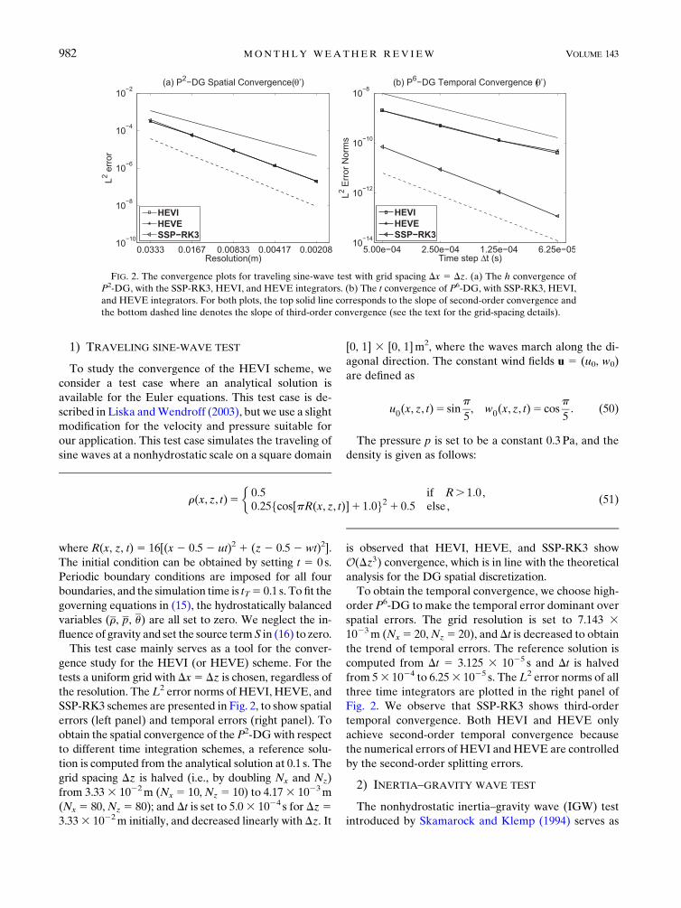
This test case mainly serves as a tool for the conver-

gence study for the HEVI (or HEVE) scheme. For the

tests a uniform grid with Dx5 Dz is chosen, regardless ofthe resolution. TheL2 error norms of HEVI, HEVE, and

SSP-RK3 schemes are presented in Fig. 2, to show spatial

errors (left panel) and temporal errors (right panel). To

obtain the spatial convergence of the P2-DGwith respect

to different time integration schemes, a reference solu-

tion is computed from the analytical solution at 0.1 s. The

grid spacing Dz is halved (i.e., by doubling Nx and Nz)

from 3.333 1022m (Nx 5 10, Nz 5 10) to 4.173 1023m

(Nx 5 80,Nz 5 80); and Dt is set to 5.03 1024 s for Dz53.333 1022m initially, and decreased linearly with Dz. It

is observed that HEVI, HEVE, and SSP-RK3 show

O(Dz3) convergence, which is in line with the theoretical

analysis for the DG spatial discretization.

To obtain the temporal convergence, we choose high-

order P6-DG to make the temporal error dominant over

spatial errors. The grid resolution is set to 7.143 31023m (Nx5 20,Nz5 20), and Dt is decreased to obtain

the trend of temporal errors. The reference solution is

computed from Dt 5 3.125 3 1025 s and Dt is halved

from 53 1024 to 6.253 1025 s. TheL2 error norms of all

three time integrators are plotted in the right panel of

Fig. 2. We observe that SSP-RK3 shows third-order

temporal convergence. Both HEVI and HEVE only

achieve second-order temporal convergence because

the numerical errors of HEVI andHEVE are controlled

by the second-order splitting errors.

2) INERTIA–GRAVITY WAVE TEST

The nonhydrostatic inertia–gravity wave (IGW) test

introduced by Skamarock and Klemp (1994) serves as

FIG. 2. The convergence plots for traveling sine-wave test with grid spacing Dx 5 Dz. (a) The h convergence of

P2-DG, with the SSP-RK3, HEVI, and HEVE integrators. (b) The t convergence of P6-DG, with SSP-RK3, HEVI,

and HEVE integrators. For both plots, the top solid line corresponds to the slope of second-order convergence and

the bottom dashed line denotes the slope of third-order convergence (see the text for the grid-spacing details).

982 MONTHLY WEATHER REV IEW VOLUME 143

a useful tool to check the accuracy of various time step-

ping schemes in a more realistic nonhydrostatic setting.

This test case obtains the grid-converged solution without

the need of a numerical diffusion.We use this experiment

to test the accuracy of theHEVI schemes for ourDG-NH

model under different aspect ratio of grid resolutions.

This test examines the evolution of a potential tempera-

ture perturbation u0, in a channel with periodic boundary

conditions on the lateral boundaries. The initial pertur-

bation (shown in Fig. 3a) radiates to the left and right

symmetrically, while being advected to the right with

a prescribed mean horizontal flow.

The parameters for the test are the same as the NH

test reported in Skamarock and Klemp (1994). The

Brunt–Väisälä frequency is given as Nf 5 0.01 s21, the

upper boundary is placed at zT 5 10km, the perturba-

tion half-width is am 5 5 km, and the initial horizontal

velocity is u 5 20m s21. The inertia–gravity waves are

produced by an initial potential temperature perturba-

tion (u0) of the following form:

u0 5 uca2m sin(pz/hc)

a2m 1 (x2 xc)2, (52)

where uc5 0.01K, hc5 10km, and xc5 100km. The (x, z)

domain is defined to be [0, 300] 3 [0, 10] km2, with no-

flux boundary conditions at the top and bottom of the

domain and periodic on the left and right sides. The

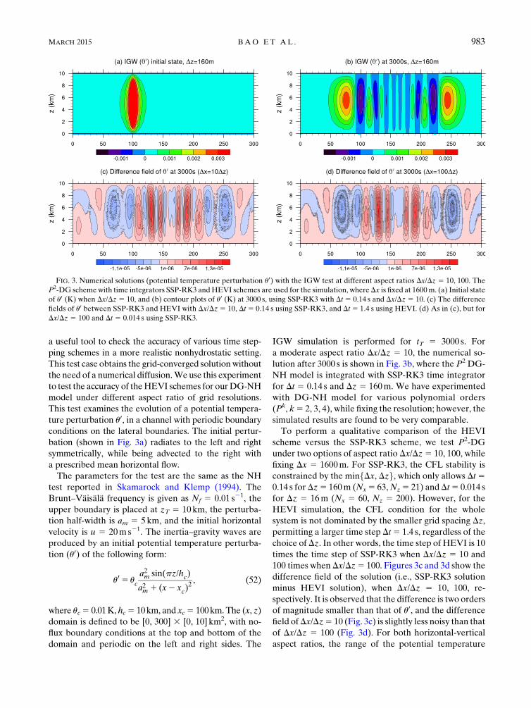
IGW simulation is performed for tT 5 3000 s. For

a moderate aspect ratio Dx/Dz 5 10, the numerical so-

lution after 3000 s is shown in Fig. 3b, where the P2 DG-

NH model is integrated with SSP-RK3 time integrator

for Dt 5 0.14 s and Dz 5 160m. We have experimented

with DG-NH model for various polynomial orders

(Pk, k5 2, 3, 4), while fixing the resolution; however, the

simulated results are found to be very comparable.

To perform a qualitative comparison of the HEVI

scheme versus the SSP-RK3 scheme, we test P2-DG

under two options of aspect ratio Dx/Dz5 10, 100, while

fixing Dx 5 1600m. For SSP-RK3, the CFL stability is

constrained by the minfDx, Dzg, which only allows Dt50.14 s forDz5 160m (Nx5 63,Nz5 21) andDt5 0.014 s

for Dz 5 16m (Nx 5 60, Nz 5 200). However, for the

HEVI simulation, the CFL condition for the whole

system is not dominated by the smaller grid spacing Dz,permitting a larger time step Dt5 1.4 s, regardless of the

choice of Dz. In other words, the time step of HEVI is 10

times the time step of SSP-RK3 when Dx/Dz 5 10 and

100 times when Dx/Dz5 100. Figures 3c and 3d show the

difference field of the solution (i.e., SSP-RK3 solution

minus HEVI solution), when Dx/Dz 5 10, 100, re-

spectively. It is observed that the difference is two orders

of magnitude smaller than that of u0, and the difference

field ofDx/Dz5 10 (Fig. 3c) is slightly less noisy than that

of Dx/Dz 5 100 (Fig. 3d). For both horizontal-vertical

aspect ratios, the range of the potential temperature

FIG. 3. Numerical solutions (potential temperature perturbation u0) with the IGW test at different aspect ratios Dx/Dz 5 10, 100. The

P2-DG schemewith time integrators SSP-RK3 andHEVI schemes are used for the simulation, whereDx is fixed at 1600m. (a) Initial state

of u0 (K) when Dx/Dz 5 10, and (b) contour plots of u0 (K) at 3000 s, using SSP-RK3 with Dt 5 0.14 s and Dx/Dz 5 10. (c) The difference

fields of u0 between SSP-RK3 and HEVI with Dx/Dz5 10, Dt5 0.14 s using SSP-RK3, and Dt5 1.4 s using HEVI. (d) As in (c), but for

Dx/Dz 5 100 and Dt 5 0.014 s using SSP-RK3.

MARCH 2015 BAO ET AL . 983

perturbation is u0 2 [21.523 1023, 2.793 1023]K, which

is fairly close to the results ofGiraldo andRestelli (2008)

and Li et al. (2013).

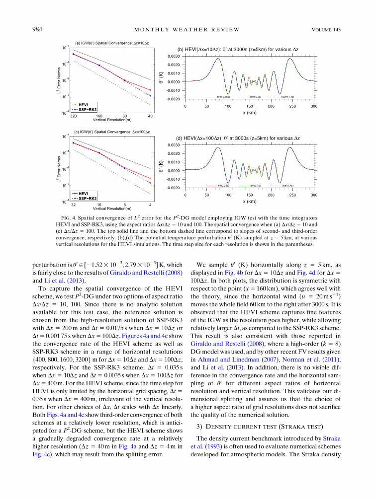
To capture the spatial convergence of the HEVI

scheme, we testP2-DG under two options of aspect ratio

Dx/Dz 5 10, 100. Since there is no analytic solution

available for this test case, the reference solution is

chosen from the high-resolution solution of SSP-RK3

with Dx 5 200m and Dt 5 0.0175 s when Dx 5 10Dz or

Dt5 0.001 75 s whenDx5 100Dz. Figures 4a and 4c showthe convergence rate of the HEVI scheme as well as

SSP-RK3 scheme in a range of horizontal resolutions

f400, 800, 1600, 3200gm for Dx5 10Dz and Dx5 100Dz,respectively. For the SSP-RK3 scheme, Dt 5 0.035 s

when Dx5 10Dz and Dt5 0.0035 s when Dx5 100Dz forDx5 400m. For theHEVI scheme, since the time step for

HEVI is only limited by the horizontal grid spacing, Dt 50.35 s when Dx 5 400m, irrelevant of the vertical resolu-

tion. For other choices of Dx, Dt scales with Dx linearly.

Both Figs. 4a and 4c show third-order convergence of both

schemes at a relatively lower resolution, which is antici-

pated for a P2-DG scheme, but the HEVI scheme shows

a gradually degraded convergence rate at a relatively

higher resolution (Dz 5 40m in Fig. 4a and Dz 5 4m in

Fig. 4c), which may result from the splitting error.

We sample u0 (K) horizontally along z 5 5 km, as

displayed in Fig. 4b for Dx 5 10Dz and Fig. 4d for Dx 5100Dz. In both plots, the distribution is symmetric with

respect to the point (x5 160km), which agrees well with

the theory, since the horizontal wind (u 5 20ms21)

moves the whole field 60km to the right after 3000 s. It is

observed that the HEVI scheme captures fine features

of the IGW as the resolution goes higher, while allowing

relatively largerDt, as compared to the SSP-RK3 scheme.

This result is also consistent with those reported in

Giraldo and Restelli (2008), where a high-order (k 5 8)

DGmodel was used, and by other recent FV results given

in Ahmad and Linedman (2007), Norman et al. (2011),

and Li et al. (2013). In addition, there is no visible dif-

ference in the convergence rate and the horizontal sam-

pling of u0 for different aspect ratios of horizontal

resolution and vertical resolution. This validates our di-

mensional splitting and assures us that the choice of

a higher aspect ratio of grid resolutions does not sacrifice

the quality of the numerical solution.

3) DENSITY CURRENT TEST (STRAKA TEST)

The density current benchmark introduced by Straka

et al. (1993) is often used to evaluate numerical schemes

developed for atmospheric models. The Straka density

FIG. 4. Spatial convergence of L2 error for the P2-DG model employing IGW test with the time integrators

HEVI and SSP-RK3, using the aspect ratios Dx/Dz5 10 and 100. The spatial convergence when (a) Dx/Dz5 10 and

(c) Dx/Dz 5 100. The top solid line and the bottom dashed line correspond to slopes of second- and third-order

convergence, respectively. (b),(d) The potential temperature perturbation u0 (K) sampled at z 5 5 km, at various

vertical resolutions for the HEVI simulations. The time step size for each resolution is shown in the parentheses.

984 MONTHLY WEATHER REV IEW VOLUME 143

current mimics the cold outflow from a convective sys-

tem and tests a model’s ability to control oscillations

when run with numerical viscosity. This test involves

evolution of a density flow generated by a cold bubble in

a neutrally stratified atmosphere. The cold bubble de-

scends to the ground and spreads out in the horizontal

direction, forming three Kelvin–Helmholtz shear in-

stability rotors along the cold front surface. This is a test

case suitable for testing the LDG diffusion option in our

DG-NH model.

The test case uses a hydrostatically balanced basic

state on a uniform potential temperature, u0 5 300K,

and adds the following perturbation in potential

temperature:

u(x, z)5

�u0 , if L(x, z). 1,

u01Du(cos[pL(x, z)]1 1)/2 otherwise,

(53)

where L(x, z)5ffiffiffiffiffiffiffiffiffiffiffiffiffiffiffiffiffiffiffiffiffiffiffiffiffiffiffiffiffiffiffiffiffiffiffiffiffiffiffiffiffiffiffiffiffiffiffiffiffiffiffiffiffiffiffiffiffiffiffi[(x2 x0)/xr]

2 1 [(z2 z0)/zr]2

q, Du 5

215K, (xr, zr) 5 (4, 2) km, and (x0, z0) 5 (0, 3) km. No-

flux boundary conditions are applied for all four bound-

aries. A dynamic viscosity of n5 75m2 s21 is used for the

diffusion (Straka et al. 1993). The diffusion terms are

treated with the LDG approach. The model is integrated

for 900 s on a domain [226.5, 26.5] 3 [0, 6.4] km2.

For an equidistant grid (Dx 5 Dz) there is no partic-

ular advantage for HEVI-DG over RK-DG in terms of

efficiency, unless w . u. The simulated potential tem-

perature u0 (K) after 900 s for the Straka density current

is shown in Figs. 5a–d, with the grid spacings successively

halved from 200 to 25m. The time step is Dt5 0.16 s for

200-m grid resolution and decreases linearly with the

grid spacing. The results shown are with the P2 version

of the DG-NH model. This test was repeated with the

high-order (Pk, k 5 3, 4) spatial discretization with

a similar resolution, and the results were visually in-

distinguishable, showing an acceptable grid conver-

gence. It is observed that three Kelvin–Helmholtz rotors

develop as the grid resolution is refined. The numerical

results are comparable to other published results

(Ahmad and Linedman 2007; Norman et al. 2011; Li

et al. 2013), despite different contour values. This test

verifies the LDG second-order diffusion in an operator-

split configuration.

Figure 5e gives the horizontal profile of the potential

temperature perturbation u0 sampled along z5 1.2 km at

the same set of the grid resolutions as in Figs. 5a–d. The

three valleys in the right panel of Fig. 5e correspond to

the three Kelvin–Helmholtz rotors in Figs. 5a–d. As the

resolution goes higher, more fine features of the current

are captured reflecting the multiscale nature of the flow.

Our results agree well with the multimoment FV

method (Li et al. 2013) and high-order DG method

(Giraldo and Restelli 2008). To compare the perfor-

mance of HEVI and SSP-RK3, the profile of potential

temperature perturbation along z 5 1.2 km for Dz 5100m is shown in Fig. 5f. The result of theHEVI scheme

is visually in line with that of SSP-RK3, which demon-

strates the robustness of the HEVI-DG combined with

the LDG diffusion.

4) SCHÄR MOUNTAIN TEST

We consider the Schär mountain test (Schär et al.2002) to evaluate the performance of our HEVI scheme

in handling complex topography. The Schär mountaintest simulates the generation of gravity waves by a con-stant horizontal flow field in a uniform stratified atmo-sphere impinging on a nonuniform mountain range. Theprofile of the mountain range is given as

h(x)5 h0 exp

2x2

a20

!cos2

pxl

, (54)

where h0 5 250m, a0 5 5000m, and l 5 4000m. The

terrain-following, height-based coordinate in (4) takes

effect in this test case and is shown in Fig. 6a. The gravity

waves are composed of two major spectral components:

the large-scale hydrostatic waves propagate deeply in

the vertical, while the small-scale nonhydrostatic waves

decay rapidly as the altitude increases.

The initial state of the atmosphere has a constant

horizontal flow of u0 5 10ms21 and the Brunt–Väisäläfrequency is Nf 5 0.01 s21. The reference potential

temperature u can be computed from (47) using u0 5280K. The simulation is carried out in the domain of

[225, 25]3 [0, 21] km2. No-flux boundary conditions are

imposed at the bottom boundary and nonreflecting

boundary conditions are used along the top, left, and

right boundaries. The sponge layers are placed in the

region of z$ 9 km with ttop 5 0.28 for the top boundary

and jxj $ 15 km with tlat 5 0.18 for the lateral outflow

boundaries. Here P3-DG is used and the grid resolution

is chosen asDx5 250mandDz5 105m (Nx5 50,Nz5 50),

which leads to Dx/Dz ’ 2. We used a different aspect

ratio than the one used in Li et al. (2013), Ullrich and

Jablonowski (2012), and Giraldo and Restelli (2008),

where Dx/Dz ’ 1, because this makes HEVI scheme

more challenging. The simulation time is tT 5 10h

(36 000 s) with Dt 5 0.125 s for the HEVI scheme and

Dt5 0.065 s for the SSP-RK3 scheme. Figures 6b and 6c

show the contours of the horizontal and vertical wind

fields at 10 h in the region [210, 10] 3 [0, 10] km2 for

visualization. No visually distinguishable difference is

observed between the results of SSP-RK3 scheme and

HEVI scheme. There is no unphysical distorted wave

MARCH 2015 BAO ET AL . 985

pattern shown in the upper level of the domain, and our

results are comparable to the other publications (Li et al.

2013; Ullrich and Jablonowski 2012; Giraldo and Restelli

2008). In addition, our handling of the complex domain

does not introduce spurious noise, as discussed in Klemp

et al. (2003).

To increase the orographic effects, the height of the

mountain in the Schär test is increased to h0 5 750m, so

that the maximum slope for the mountain is about 55%

(Simarro et al. 2013). The purpose of this test is to make

a close comparison between HEVI and SSP-RK3 in a rel-

atively extreme case. The grid resolution and boundary

conditions for this experiment remain the same as in the

Schär test, and themodel is integrated for a short period oft 5 1800 s, with HEVI as well as SSP-RK3 schemes. The

terrain-following coordinate is shown in Fig. 6d, which is

more curved (with sharp gradients) than the case shown in

Fig. 6a. For the HEVI scheme, Dt5 0.125 s, which is twice

FIG. 5. The plots of potential temperature perturbation u0 (K) for the Straka density current test on a uniform grid Dx5Dzwith P2-DG

schemes for 900-s integration. (a)–(d) The contour plots of u0 using HEVI in a range of resolutions from 200 to 25m. Time step Dt5 0.16 s

for 200-m grid resolution, and is otherwise proportional with the grid resolution. The contour values (K) are in the range of [29.5, 0.5] with

an increment 1.0. (e),(f) The sampling of u0 at z5 1.2 km are shown, where (e) shows the plots corresponding to the resolutions as used in

(a)–(d), and the associated time step is given in the parentheses. In (f) HEVI and SSP-RK3 schemes are compared at a resolution of 100m.

986 MONTHLY WEATHER REV IEW VOLUME 143

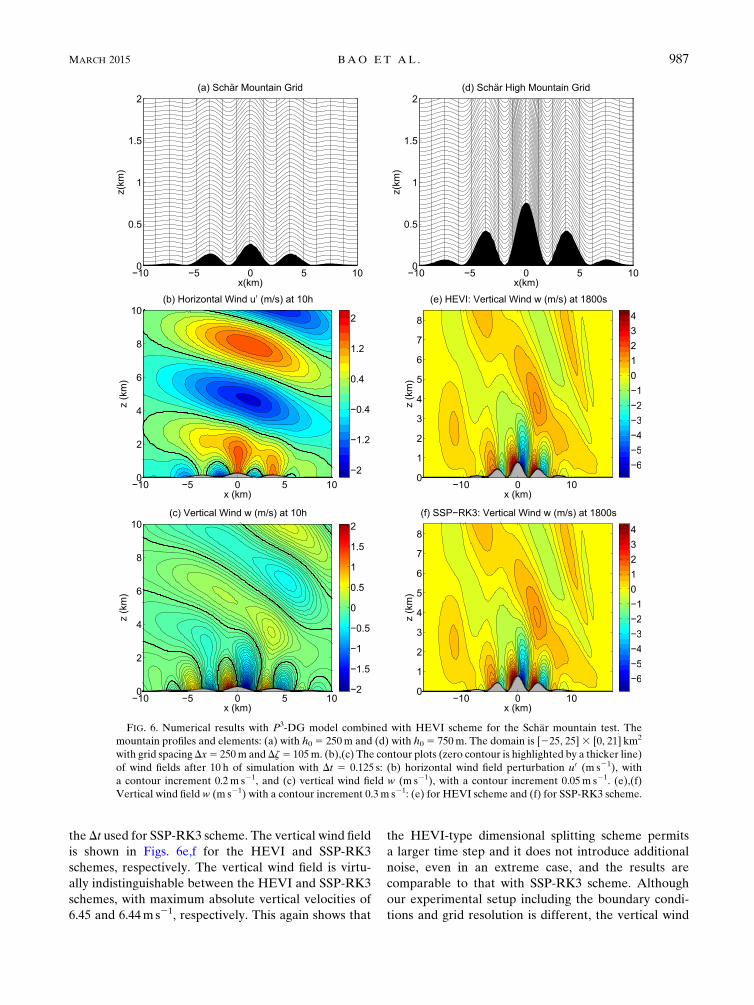
the Dt used for SSP-RK3 scheme. The vertical wind field

is shown in Figs. 6e,f for the HEVI and SSP-RK3

schemes, respectively. The vertical wind field is virtu-

ally indistinguishable between the HEVI and SSP-RK3

schemes, with maximum absolute vertical velocities of

6.45 and 6.44ms21, respectively. This again shows that

the HEVI-type dimensional splitting scheme permits

a larger time step and it does not introduce additional

noise, even in an extreme case, and the results are

comparable to that with SSP-RK3 scheme. Although

our experimental setup including the boundary condi-

tions and grid resolution is different, the vertical wind

FIG. 6. Numerical results with P3-DG model combined with HEVI scheme for the Schär mountain test. Themountain profiles and elements: (a) with h0 5 250m and (d) with h0 5 750m. The domain is [225, 25]3 [0, 21] km2

with grid spacingDx5 250m and Dz5 105m. (b),(c) The contour plots (zero contour is highlighted by a thicker line)

of wind fields after 10 h of simulation with Dt 5 0.125 s: (b) horizontal wind field perturbation u0 (m s21), with

a contour increment 0.2m s21, and (c) vertical wind field w (m s21), with a contour increment 0.05m s21. (e),(f)

Vertical wind field w (m s21) with a contour increment 0.3m s21: (e) for HEVI scheme and (f) for SSP-RK3 scheme.

MARCH 2015 BAO ET AL . 987

fields shown in Figs. 6e,f are similar to the corresponding

Fig. 3 of Simarro et al. (2013).

6. Summary and conclusions

We have proposed a moderate-order discontinuous

Galerkin nonhydrostatic (DG-NH) model based on the

compressible Euler equations in a 2D (x, z) Cartesian

plane, with a simple operator-splitting time integration

scheme. The model uses a terrain-following height-based

coordinate to handle the orography. For the atmospheric

simulation on the nonhydrostatic scale, a high aspect ratio

between the horizontal and vertical spatial discretiza-

tion imposes a stringent restriction on the explicit time

step size for the Euler system. To alleviate the dominant

effect due to large horizontal–vertical aspect ratio, the

so-called horizontally explicit and vertically implicit

(HEVI) scheme via the Strang splitting is proposed and

studied in ourDG-NHmodel. TheHEVI time-integration

scheme avoids the tiny time step limitations, inflicted by

the vertical grid spacing (Dz � Dx), and, therefore, theoverall CFL restriction on the time step is mainly de-

termined by the horizontal grid spacing (Dx).The accuracy of our HEVI DG-NH model is tested

under a suite of NH benchmark test cases. The numer-

ical results, which are in agreement with those in liter-

ature, show that the HEVI scheme is robust and capable

of relaxing the CFL constraint to the horizontal grid

spacing and yields accurate simulations, even though the

vertical grid spacing is greatly smaller than the hori-

zontal (Dx/Dz 5 10, 100). As expected, a second-order

temporal convergence is observed with the HEVI

scheme, and a third-order spatial convergence is obtained

with the HEVI scheme as well as the SSP-RK3 scheme,

which is consistent with the P2-DG discretization. We

have also implemented an LDG-type second-order dif-

fusion in a dimension-split manner to be consistent with

the HEVI formulation. The LDG diffusion effectively

eliminates the small-scale noise for the model and stabi-

lizes the flow field, as is shown in the Straka density

current test. Moreover, in the presence of orography

(Schär mountain test), no spurious wave pattern or noiseis detected from the results of our HEVI scheme, and thenumerical simulation is visually identical to that of theSSP-RK3 scheme.The HEVI scheme is a practical option and competi-

tive approach for global NH atmospheric modeling,

since the existing solver of the horizontal dynamics can

be greatly recycled as done in a typical split-explicit case

when implemented in a full 3D domain. Here we dem-

onstrate that it is a viable option for the high-order DG

method as well. However, the efficiency of the HEVI

scheme mainly depends on the performance of the 1D

implicit solver. Proper preconditioning is a possible

remedy for accelerating the Newton–Krylov Jacobian-

free solver, and work in this direction is progressing. Our

ultimate goal is to implement the HEVI-DG formula-

tion in the High-Order Method Modeling Environment

(HOMME) developed at NCAR, to extend it as a NH

framework. The attractive features of HOMME (ex-

cellent parallel efficiency) can be exploited for the re-

sulting NH dynamical core when HEVI-DG scheme is

implemented. Further investigation will be continued on

the application of the HEVI time-split scheme in the

HOMME framework.

Acknowledgments. The authors thank two anony-

mous reviewers for the insightful comments that

improved the manuscript, and Dr. Michael Toy for

a thorough internal review. The first author would like

to thank Prof. Henry M. Tufo for his support and en-

couragement. RDN would like to thank Dr. Seoleun

Shin and KIAPS, Seoul, South Korea, for their support.

This work was partially supported by the DOE BER

Program under Award DE-SC0006959.

APPENDIX

Diffusion

Consider the following scalar advection-diffusion

equation on an element Ve, with the known (constant)

diffusion coefficient n (m2 s21):

›U

›t1$ � F(U)5 n=2U . (A1)

We summarize the application of LDGdiffusion process

in the following steps. [In the following process the

subscript (�)h is dropped for simplicity.]

1) The key idea of the LDG approach is the introduc-

tion of a local auxiliary variable q 5 n$U, and

rewriting the above problem as a first-order system:

q2 n$U5 0, (A2)

›U

›t1$ � F(U)2$ � q5 0. (A3)

2) For the LDG method, Let the numerical fluxes U*,

q* in (A6) be evaluated in terms of jump [�] and

central f�g fluxes, defined as follows:

U*5 fUg1b � [U], q*5 fqg2b[q]2hk[U],

(A4)

fUg5 (U1 1U2)/2, [U]5 (U2 2U1)n;

fqg5 (q1 1 q2)/2, [q]5 (q22 q1) � n .

988 MONTHLY WEATHER REV IEW VOLUME 143

3) Discretize the above system in (A2) and (A3) using

the weak formulation (Green’s method). This is

done by first multiplying by a vector test function

F 2 Vd(V) (d is the dimension of the problem) in

(A2) and integrating by parts:ðVq �FdV5 n

�ð›V

U*F � n ds2

ðVU$ �FdV

�.

(A5)

4) The final weak formulation for the advection-

diffusion equation (A1) is obtained by using a test

function [u 2 V(V)], the Lax–Friedrichs flux F̂, and

combining (A5):

›

›t

ðVUu dV2

ðVF(U) � $u dV1

ð›V

F̂(U) � nu ds

1 n

ðVq � $u dV2 n

ð›V

q* � nu ds5 0.

(A6)

5) In practice this is done in two stages. First, evaluate q

in (A5) using the above fluxes and then evaluate (A6).

Note that various second-order diffusions can be

formulated by carefully choosing the parameter valuesb

and hk, which are BR2, Bauman–Oden, and ‘‘flip-flop,’’

etc. [see Cockburn and Shu (1998) for multiple variants

of theLDGmethod]. The constantsb5 n/2 andhk5 0 are

set for most test cases considered herein, nevertheless,

other options are available in the DG-NH model.

REFERENCES

Ahmad, N., and J. Linedman, 2007: Euler solutions using flux-

based wave decomposition. Int. J. Numer. Methods Fluids, 54,

47–72, doi:10.1002/fld.1392.

Alexander, R., 1977: Diagonally implicit Runge–Kutta methods

for stiff O.D.E.’s. SIAM J. Numer. Anal., 14, 1006–1021,

doi:10.1137/0714068.

Ascher, U. M., S. J. Ruuth, and R. J. Spiteri, 1997: Implicit-explicit

Runge–Kutta methods for time-dependent partial differential

equations. Appl. Numer. Math., 25, 151–167, doi:10.1016/

S0168-9274(97)00056-1.

Bao, L., R. D. Nair, and H. M. Tufo, 2014: A mass and momentum

flux-form high-order discontinuous Galerkin shallow water

model on the cubed-sphere. J. Comput. Phys., 271, 224–243,

doi:10.1016/j.jcp.2013.11.033.

Brdar, S., M. Baldauf, A. Dedner, and R. Klöfkorn, 2013: Com-

parison of dynamical cores for NWP models: Comparison of

COSMO and Dune. Theor. Comput. Fluid Dyn., 27, 453–472,

doi:10.1007/s00162-012-0264-z.

Butcher, J. C., 1987: The Numerical Analysis of Ordinary Differ-

ential Equations: Runge–Kutta and General Linear Methods.

John Wiley & Sons Inc., 528 pp.

Clark, T. L., 1977: A small-scale dynamics model using a terrain-

following coordinate transformation. J. Comput. Phys., 24,

186–215, doi:10.1016/0021-9991(77)90057-2.

Cockburn, B., 1997: An introduction to the discontinuous-Galerkin

method for convection-dominated problems. Lecture Notes in

Mathematics: Advanced Numerical Approximation of Non-

linear Hyperbolic Equations, A. Quarteroni, Ed., Vol. 1697,

Springer, 151–268.

——, and C.-W. Shu, 1998: The local discontinuous Galerkin for

convection diffusion systems. SIAMJ. Numer. Anal., 35, 2440–

2463, doi:10.1137/S0036142997316712.

Dennis, J. M., and Coauthors, 2012: CAM-SE: A scalable spectral

element dynamical core for the Community Atmosphere

Model. Int. J. High Perform. Comput. Appl., 26, 74–89,

doi:10.1177/1094342011428142.

Durran, D. R., 1999: Numerical Methods for Wave Equations in

Geophysical Fluid Dynamics. Springer, 465 pp.

——, and J. B. Klemp, 1983: A compressible model for the simula-

tion of moist mountain waves.Mon. Wea. Rev., 111, 2341–2361,doi:10.1175/1520-0493(1983)111,2341:ACMFTS.2.0.CO;2.

Gal-Chen, T., and R. C. Sommerville, 1975: On the use of a co-

ordinate transformation for the solution of Navier–Stokes.

J. Comput. Phys., 17, 209–228, doi:10.1016/0021-9991(75)90037-6.

Giraldo, F. X., and M. Restelli, 2008: A study of spectral element

and discontinuous Galerkin methods for the Navier–Stokes

equations in nonhydrostatic mesoscale atmospheric modeling:

Equation sets and test cases. J. Comput. Phys., 227, 3849–3877,

doi:10.1016/j.jcp.2007.12.009.

——, J. F. Kelly, and E. M. Constantinescu, 2013: Implicit-explicit

formulations of a three-dimensional nonhydrostatic unified

model of the atmosphere (NUMA). SIAM J. Sci. Comput., 35,

B1162–B1194, doi:10.1137/120876034.

Gottlieb, S., C.-W. Shu, and E. Tadmor, 2001: Strong stability-

preserving high-order time discretization methods. SIAM

Rev., 43, 89–112, doi:10.1137/S003614450036757X.

Guo, W., R. D. Nair, and J.-M. Qiu, 2014: A conservative semi-

Lagrangian discontinuous Galerkin scheme on the cubed

sphere. Mon. Wea. Rev., 142, 457–475, doi:10.1175/

MWR-D-13-00048.1.

Karniadakis, G. E., and S. Sherwin, 2005: Spectral/hp Element

Methods for Computational Fluid Dynamics. Oxford Univer-

sity Press, 657 pp.

Klemp, J. B., 2011: A terrain-following coordinate with smoothed

coordinate surfaces.Mon.Wea.Rev., 139, 2163–2169, doi:10.1175/MWR-D-10-05046.1.

——,W.C. Skamarock, andO. Fuhrer, 2003:Numerical consistency

of metric terms in terrain-following coordinates. Mon. Wea.

Rev., 131, 1229–1239, doi:10.1175/1520-0493(2003)131,1229:

NCOMTI.2.0.CO;2.

Knoll, D. A., andD. E. Keyes, 2004: Jacobian-free Newton–Krylov

methods: A survey of approaches and applications. J. Comput.

Phys., 193, 357–397, doi:10.1016/j.jcp.2003.08.010.

Li, X., C. Chen, X. Shen, and F. Xiao, 2013: A multimoment con-

strained finite-volume model for nonhydrostatic atmospheric

dynamics. Mon. Wea. Rev., 141, 1216–1240, doi:10.1175/

MWR-D-12-00144.1.

Liska, R., and B.Wendroff, 2003: Comparison of several difference

schemes on 1D and 2D test problems for the Euler equa-

tions. SIAM J. Sci. Comput., 25, 995–1017, doi:10.1137/

S1064827502402120.

Lock, S. J., N. Wood, and H. Weller, 2014: Numerical analyses of

Runge–Kutta implicit-explicit schemes for horizontally explicit,

vertically implicit solutions of atmospheric models. Quart.

J. Roy. Meteor. Soc., 140, 1654–1669, doi:10.1002/qj.2246.

Melvin, T., M. Dubal, N. Wood, A. Staniforth, and M. Zerroukat,

2010: An inherently mass-conserving iterative semi-implicit

MARCH 2015 BAO ET AL . 989

semi-Lagrangian discretization of the non-hydrostatic

vertical-slice equations. Quart. J. Roy. Meteor. Soc., 136,

799–814, doi:10.1002/qj.603.

Michalakes, J., and Coauthors, 2007: WRF nature run. Proc.

2007 ACM/IEEE Conf. on Supercomputing, 2007 (SC’ 07),

Reno, NV, ACM; IEEE, 1–6, doi:10.1145/1362622.1362701.

Nair, R. D., 2009: Diffusion experiments with a global discontin-

uous Galerkin shallow-water model. Mon. Wea. Rev., 137,3339–3350, doi:10.1175/2009MWR2843.1.

——, H.-W. Choi, and H. M. Tufo, 2009: Computational aspects of

a scalable high-order discontinuous Galerkin atmospheric

dynamical core. Comput. Fluids, 38, 309–319, doi:10.1016/

j.compfluid.2008.04.006.

——, M. N. Levy, and P. H. Lauritzen, 2011: Emerging numerical

methods for atmospheric modeling.Numerical Techniques for

Global Atmospheric Models, P. H. Lauritzen et al., Eds., Vol.

80, Springer-Verlag, 189–250.

Norman, M. R., R. D. Nair, and F. H. M. Semazzi, 2011: A low

communication and large time step explicit finite-volume

solver for non-hydrostatic atmospheric dynamics. J. Comput.

Phys., 230, 1567–1584, doi:10.1016/j.jcp.2010.11.022.

Prusa, J., P. Smolarkiewicz, and A. Wyszogrodzki, 2008: EULAG,

a computational model for multiscale flows. Comput. Fluids,

37, 1193–1207, doi:10.1016/j.compfluid.2007.12.001.

Restelli, M., and F. Giraldo, 2009: A conservative discontinuous

Galerkin semi-implicit formulation for the Navier–Stokes

equations in nonhydrostatic mesoscale modeling. SIAM J. Sci.

Comput., 31, 2231–2257, doi:10.1137/070708470.

Saad, Y., andM.H. Schultz, 1986: GMRES:A generalizedminimal

residual algorithm for solving nonsymmetric linear systems.

SIAM J. Sci. Stat. Comput., 7, 856–869, doi:10.1137/0907058.

Satoh, M., 2002: Conservative scheme for the compressible non-

hydrostatic models with the horizontally explicit and vertically

implicit time integration scheme.Mon.Wea. Rev., 130, 1227–1245,doi:10.1175/1520-0493(2002)130,1227:CSFTCN.2.0.CO;2.

Schär, C., D. Leuenberger, O. Fuhrer, D. Luthic, and C. Girard, 2002:

A new terrain-following vertical coordinate formulation for at-

mospheric prediction models. Mon. Wea. Rev., 130, 2459–2480,

doi:10.1175/1520-0493(2002)130,2459:ANTFVC.2.0.CO;2.

Simarro, J., V. Homar, and G. Simarro, 2013: A non-hydrostatic

global spectral dynamical core using a height-based vertical

coordinate.Tellus, 65A, 20270, doi:10.3402/tellusa.v65i0.20270.

Skamarock, W., and J. Klemp, 1994: Efficiency and accuracy of the

Klemp–Wilhelmson time-splitting technique.Mon.Wea. Rev.,

122, 2623–2630, doi:10.1175/1520-0493(1994)122,2623:

EAAOTK.2.0.CO;2.

——, and ——, 2008: A time-split nonhydrostatic atmos-

pheric model for weather research and forecasting applica-

tions. J. Comput. Phys., 227, 3465–3485, doi:10.1016/

j.jcp.2007.01.037.

——, ——, M. G. Duda, L. D. Flower, S.-H. Park, and T. D.

Ringler, 2012: A multiscale nonhydrostatic atmospheric

model using centroidal Voronoi tesselations and C-grid

staggering. Mon. Wea. Rev., 140, 3090–3105, doi:10.1175/

MWR-D-11-00215.1.

St-Cyr,A., andD.Neckels, 2009:A fully implicit Jacobian-free high-

order discontinuous Galerkin mesoscale flow solver. Lecture

Notes in Computer Science, G. Allen et al., Eds., Vol. 5545,

Springer-Verlag, 243–252, doi:10.1007/978-3-642-01973-9_28.

Straka, J.,R.Wilhelmson,L.Wicker, J.Anderson, andK.Droegemeier,

1993: Numerical solutions of a non-linear density current: A

benchmark solution and comparisons. Int. J. Numer. Methods

Fluids, 17, 1–22, doi:10.1002/fld.1650170103.Strang, G., 1968: On the construction and comparison of difference

schemes. SIAM J. Numer. Anal., 5, 506–517, doi:10.1137/

0705041.

Tomita, H., K. Goto, and M. Satoh, 2008: A new approach to

atmospheric general circulation model: Global cloud resolv-

ing model NICAM and its computational performance. SIAM

J. Sci. Comput., 30, 2755–2776, doi:10.1137/070692273.Toro, E. F., 1999: Riemann Solvers and Numerical Methods for

Fluid Dynamics: A Practical Introduction. 2nd ed. Springer-

Verlag, 724 pp.

Toy, M. D., and D. A. Randall, 2009: Design of a nonhydrostatic

atmospheric model based on a generalized vertical co-

ordinate. Mon. Wea. Rev., 137, 2305–2330, doi:10.1175/

2009MWR2834.1.

Ullrich, P., and C. Jablonowski, 2012: Operator-split Runge–

Kutta–Rosenbrock methods for nonhydrostatic atmospheric

models. Mon. Wea. Rev., 140, 1257–1284, doi:10.1175/

MWR-D-10-05073.1.

Weller, H., S.-J. Lock, and N. Wood, 2013: Runge–Kutta IMEX

schemes for the Horizontally Explicit/Vertically Implicit

(HEVI) solution of wave equations. J. Comput. Phys., 252,

365–381, doi:10.1016/j.jcp.2013.06.025.

Zhang, Y., and R. D. Nair, 2012: A nonoscillatory discontinuous

Galerkin transport scheme on the cubed sphere. Mon. Wea.

Rev., 140, 3106–3126, doi:10.1175/MWR-D-11-00287.1.

990 MONTHLY WEATHER REV IEW VOLUME 143