HOMOGENEOUS TRANSCODING OF HEVC (H.265) - … TRANSCODING OF HEVC (H.265) ... MPEG-4 visual and...

HOMOGENEOUS TRANSCODING OF HEVC (H.265)

by

NINAD GOREY

Presented to the Faculty of the Graduate School of

The University of Texas at Arlington in Partial Fulfillment

of the Requirements

for the Degree of

MASTER OF SCIENCE IN ELECTRICAL ENGINEERING

THE UNIVERSITY OF TEXAS AT ARLINGTON

May 2017

ACKNOWLEDGEMENTS

First of all, I am particularly grateful to my advisor Dr. K. R. Rao for his

unwavering support, encouragement and supervision throughout this work. He has

been a constant source of inspiration towards the completion of this research work.

Additionally, I would like to thank Dr. Kambiz Alavi and Dr. Jonathan Bredow

for serving as members of my graduate committee.

I would like to thank my Multimedia Processing Lab mates especially Harsha

for providing valuable suggestions during my research work.

Finally, I would like to thank God, my family members and friends for believing

in me and supporting me in this undertaking. Special thanks to my roommates

Swanand and Pratik for their support and understanding. I wish for their continued

support in future.

April 26, 2017

ABSTRACT

HOMOGENEOUS TRANSCODING OF HEVC (H.265)

Ninad Gorey, MS

The University of Texas at Arlington, 2017

Supervising Professor: K. R. Rao

Video transcoding is an essential tool to promote inter-operability between different

video communication systems. This thesis presents a cascaded architecture for

homogeneous transcoding of High Efficiency Video Coding.

Cascaded Transcoding model decodes the input video sequence and follows

the procedure of reference encoder, with the difference being a higher QP value. The

encoder will code the sequence with the goal of achieving highest coding

performance, and since the encoder is not restricted by any means, it is reasonable to

assume that the coding performance is the best possible transcoding performance.

H.265 is the latest video coding standard which supports encoding videos with

wide range of resolutions, starting from low resolution to beyond High Definition i.e.

4k or 8k. H.265 also known as HEVC was preceded by H.264/AVC which is a very well

established and widely used standard in industry and finds its applications in

broadcast and multimedia telephony.

HEVC achieves high coding efficiency at the cost of increased complexity and

not all devices have complex hardware capable enough to process the HEVC bit

stream. So, to enable HEVC content playing capabilities on heterogeneous device

platforms homogeneous transcoding of HEVC is necessary.

Different transcoding architectures are investigated and architecture with

optimum performance is implemented and studied as part of this research. The

architecture is implemented using existing reference software of H.265. Different

quality metrics (PSNR, Bitrate, Bitrate Ratio, Transcoding time) are measured for the

proposed scheme using different test sequences and conclusions are drawn based on

these results.

Contents ACKNOWLEDGEMENTS ................................................................................................. 3

ABSTRACT ...................................................................................................................... 4

1. Introduction .............................................................................................................. 8

1.1 Thesis Scope ........................................................................................................ 9

1.2 Thesis Organization ............................................................................................. 9

2. Video Coding ........................................................................................................... 10

2.1 Overview of Digital Video ................................................................................. 10

2.2 Need for Video Compression ............................................................................ 12

2.3 Video Coding Basics .......................................................................................... 13

2.3.1 Prediction Model ....................................................................................... 14

2.3.2 Spatial Model ............................................................................................. 15

2.3.3 Statistical Model ........................................................................................ 16

2.4 Video Quality Measurement ............................................................................. 17

2.4.1 Peak Signal-to-Noise Ratio ......................................................................... 17

2.4.2 Bit Rate (R) and Bit Rate Ratio (r) .............................................................. 17

3. Overview of High Efficiency Video Coding .............................................................. 18

3.1 Introduction ...................................................................................................... 18

3.2 Profiles and Levels ............................................................................................ 19

3.3 Encoder and Decoder........................................................................................ 21

3.3.1 Coding Tree Units ....................................................................................... 23

3.3.2 Coding Units ............................................................................................... 23

3.3.3 Prediction Modes ....................................................................................... 24

3.3.4 Prediction Units ......................................................................................... 25

3.3.5 Transform Units ......................................................................................... 26

3.3.6 Motion Compensation ............................................................................... 27

3.3.7 Entropy Coding ........................................................................................... 27

3.3.8 Sample Adaptive Offset ............................................................................. 27

3.4 Summary ........................................................................................................... 28

4. Transcoding ............................................................................................................. 29

4.1 Introduction ...................................................................................................... 29

4.2 Need for Transcoding ........................................................................................ 29

4.3 Video Transcoding Challenges .......................................................................... 30

4.3.1 Distortion ................................................................................................... 30

4.3.2 Computational Complexity ........................................................................ 30

4.4 Video Transcoding Methods ............................................................................. 31

4.4.1 Homogeneous Transcoding ....................................................................... 32

4.4.2 Heterogeneous Transcoding ...................................................................... 33

4.5 Transcoding Architecture .................................................................................. 35

4.5.1 Open-loop Architecture ............................................................................. 36

4.5.2 Closed-loop Architecture ........................................................................... 36

4.5.3 Cascaded pixel domain Architecture ......................................................... 37

4.6 Comparison of Transcoding Architectures ....................................................... 38

4.7 Related Work .................................................................................................... 39

4.8 Proposed Transcoder ........................................................................................ 41

4.9 Summary ........................................................................................................... 42

5. Results ..................................................................................................................... 43

5.1 Quality Metrics for Cascaded Transcoder Implementation ............................. 43

5.2 Peak-Signal-to-Noise-Ratio (PSNR) versus Quantization Parameter (QP) ........ 46

5.3 Bit Rate Ratio (r) vs Quantization Parameter (QP) ........................................... 49

5.4 Transcoding Time (sec) vs Quantization Parameter (QP) ................................. 52

5.5 Rate Distortion (R-D) Plot ................................................................................. 55

5.6 Comparison of Input video frame and transcoded video frame ...................... 56

6. Conclusions ............................................................................................................. 59

6.1 Overview of Transcoder performance .............................................................. 59

6.2 Future Work ...................................................................................................... 59

A. Test Sequences ....................................................................................................... 61

B. Test Environment .................................................................................................... 64

C. Acronyms ................................................................................................................ 65

References .................................................................................................................. 68

1. Introduction

Video content is produced daily through variety of electronic devices, however,

storing and transmitting video signals in raw format are impractical due to its

excessive resource requirement. Today popular video coding standards such as

MPEG-4 visual and H.264/AVC [28] are used to compress the video signals before

storing and transmitting. Accordingly, efficient video coding plays an important role

in video communications. While video applications become wide-spread, there is a

need for high compression and low complexity video coding algorithms that preserve

the image quality.

Standard organizations ISO, ITS, VCEG of ITU-T with collaboration of many

companies have developed video coding standards in the past to meet video coding

requirements of the modern day. The Advanced Video Coding (AVC/H.264) standard

is the most widely used video coding method [29]. AVC is commonly known to be one

of the major standards used in Blue Ray devices for video compression. It is also widely

used by video streaming services, TV broadcasting, and video conferencing

applications. Currently the most important development in this area is the

introduction of H.265/HEVC standard which has been finalized in January 2013 [1].

The aim of standardization is to produce video compression specification that can

compress video twice as effectively as H.264/AVC standard in terms of quality [1].

There are a wide range of platforms that receive digital video. TVs, personal

computers, mobile phones, tablets and iPads each have different computational,

display, and connectivity capabilities, thus video must be converted to meet the

specifications of target platform. This conversion is achieved through video

transcoding. For transcoding, straightforward solution is to decode the compressed

video signal and re-encode it to the target compression format, but this process is

computationally complex. Particularly in real-time applications, there is a need to

exploit the information that is already available through the compressed video bit-

stream to speed-up the conversion [2].

1.1 Thesis Scope

The objective of this thesis is to implement efficient transcoding architecture for

homogeneous transcoding of HEVC. Performing full decode and re-encode of the

incoming bit stream, the transcoded bit stream will be evaluated based on

performance metrics and transcoder performance on various video sequences will be

investigated. The implementation of the transcoding model is developed using the

reference software of HEVC [42].

1.2 Thesis Organization

This thesis is organized as follows:

Chapter 2 presents the general description of video coding. It explains the need for

compression of video signals and video coding basics. It also defines various

performance metrics used in this thesis.

Chapter 3 describes the overview of HEVC, profiles and levels along with some key

features of HEVC coding design.

Chapter 4 describes the need for transcoding, various transcoding architectures and

the proposed homogeneous transcoder.

Chapter 5 presents results and graphs for the different test sequences and

quantization parameters. RD plots are displayed to understand the transcoder

performance for different sequences.

Chapter 6 discusses conclusions that can be drawn from results obtained in chapter 5

and explores future work in the same direction.

2. Video Coding

2.1 Overview of Digital Video

Digital video is a discrete representation of real world images sampled in spatial and

temporal domains. In temporal domain samples are commonly taken at the rate of

25, 30, or more, frames per second. Each video frame is a still image composed of

pixels bounded by spatial dimensions. Typical video spatial-resolutions are 1280 x 720

(HD) or 1920 x 1080 (Full HD) pixels.

A pixel has one or more components per color space. Commonly used color

spaces are RGB and YCbCr. RGB color space describes the relative proportions of Red,

Blue, and Green to define a color in the RGB pixel domain. 8 bits are required for each

of the RGB components which is 24-bits in total. The YCbCr color space is developed

with the human visual system in mind. Human visual perception is less sensitive to

colors compared to brightness, by exploiting this fact the number of chroma samples

are reduced for every luma sample without sacrificing the perceived quality of the

image. This conversion from RGB to YCbCr reduces the number of bits required to

represent the pixel. In YCbCr color space, Y is the luminance and it is calculated as the

weighted average (𝑘𝑟, 𝑘𝑔, 𝑘𝑏) of RGB:

𝑌 = 𝑘𝑟 𝑅 + 𝑘𝑔 𝐺 + 𝑘𝑏 𝐵

The color information is calculated as the difference between Y and RGB:

𝐶𝑟 = 𝑅 − 𝑌

𝐶𝑔 = 𝐺 − 𝑌

𝐶𝑏 = 𝐵 − 𝑌

Observe that since Cr + Cg + Cb is constant, storing Cr and Cb is sufficient. As mentioned

before, YCbCr frames can have pixels sampled with different resolution for luma and

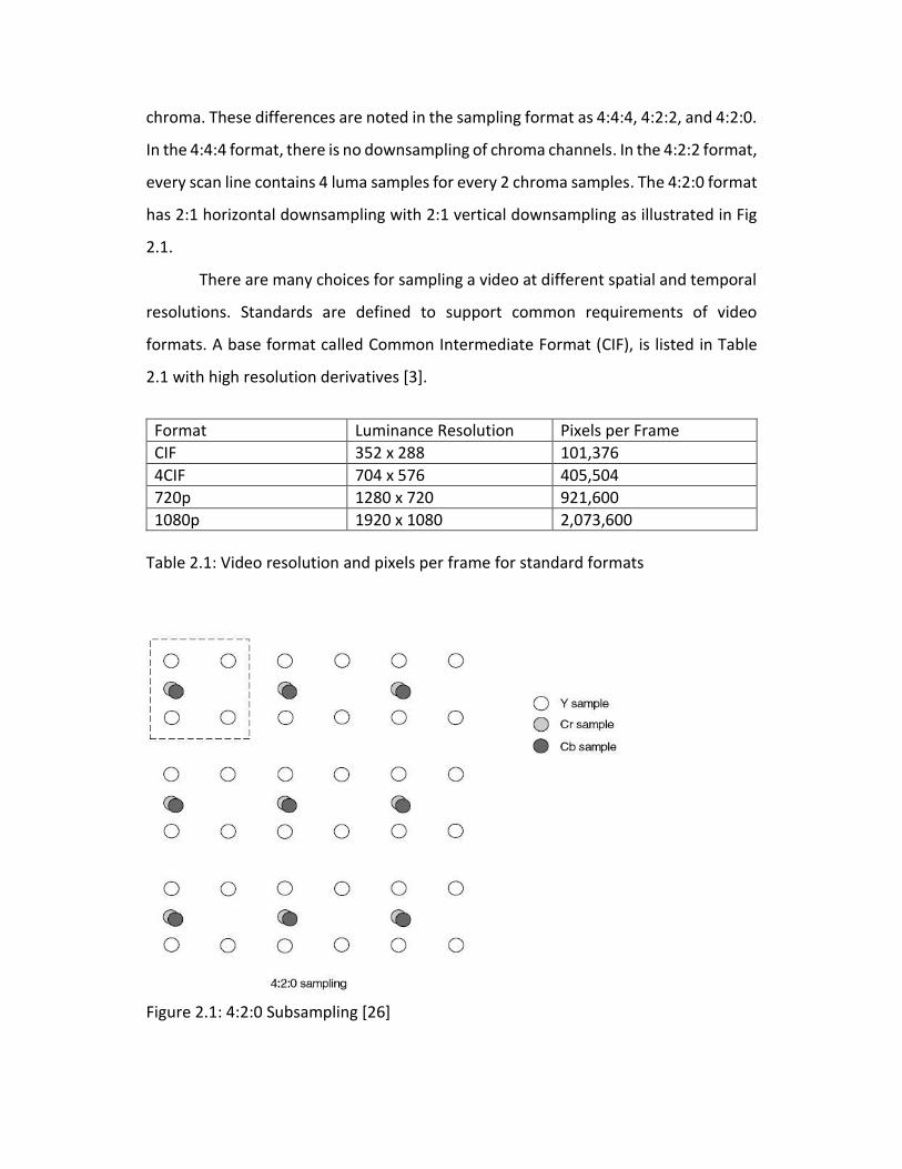
chroma. These differences are noted in the sampling format as 4:4:4, 4:2:2, and 4:2:0.

In the 4:4:4 format, there is no downsampling of chroma channels. In the 4:2:2 format,

every scan line contains 4 luma samples for every 2 chroma samples. The 4:2:0 format

has 2:1 horizontal downsampling with 2:1 vertical downsampling as illustrated in Fig

2.1.

There are many choices for sampling a video at different spatial and temporal

resolutions. Standards are defined to support common requirements of video

formats. A base format called Common Intermediate Format (CIF), is listed in Table

2.1 with high resolution derivatives [3].

Format Luminance Resolution Pixels per Frame

CIF 352 x 288 101,376

4CIF 704 x 576 405,504

720p 1280 x 720 921,600

1080p 1920 x 1080 2,073,600

Table 2.1: Video resolution and pixels per frame for standard formats

Figure 2.1: 4:2:0 Subsampling [26]

2.2 Need for Video Compression

The high bit rates that result from the various types of digital video make their

transmission through their intended channels very difficult. High resolution videos

captured by HD cameras and HD videos on the internet would require bandwidth and

storage space if used in the raw format. Even if high bandwidth technology (e.g. fiber-

optic cable) was in place, the per-byte-cost of transmission would have to be very low

before it would be feasible to use it for transmission of enormous amounts of data

required by HDTV. Finally, even if the storage and transportation problems of digital

video were overcome, the processing power needed to manage such volumes of data

would make the receiver hardware very expensive. Also, because of the growing use

of internet, online streaming services and multimedia mobile devices it is required to

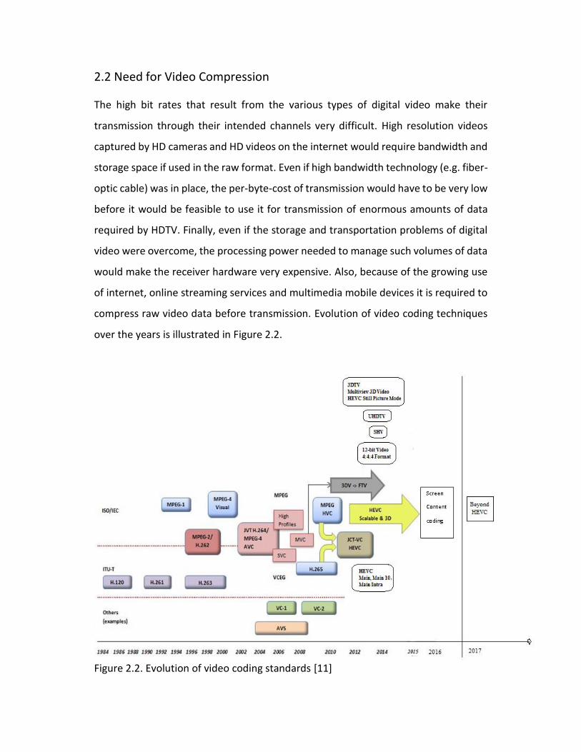
compress raw video data before transmission. Evolution of video coding techniques

over the years is illustrated in Figure 2.2.

Figure 2.2. Evolution of video coding standards [11]

2.3 Video Coding Basics

According to Table 2.1, number of required pixels per frame is huge, therefore storing

and transmitting raw digital video requires excessive amounts of space and

bandwidth. To reduce video bandwidth requirements compression methods are used.

In general, compression is defined as encoding data to reduce the number of bits

required to present the data. Compression can be lossless or lossy. A lossless

compression preserves the original quality so that after decompression the original

data is obtained, whereas, in lossy compression, while offering higher compression

ratio, the decompressed data is not equal to the original data. Video data is

compressed and decompressed with the techniques discussed under the term video

coding, with compressor often denoted as enCOder and decompressor as DECoder,

which collectively form the term CODEC. Therefore, a CODEC is the collection of

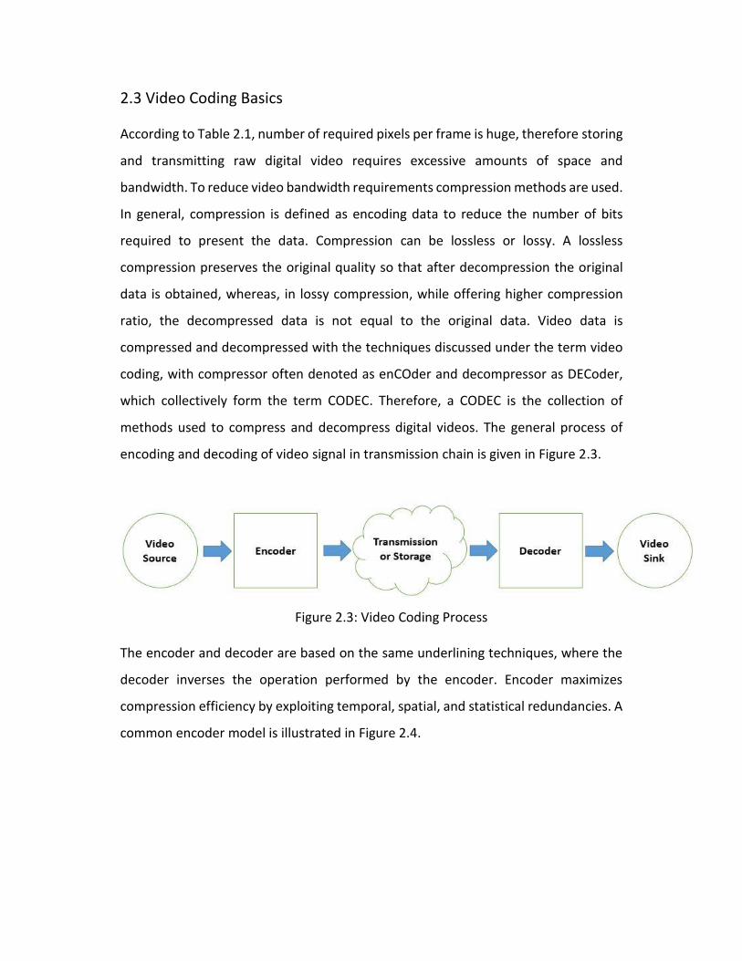
methods used to compress and decompress digital videos. The general process of

encoding and decoding of video signal in transmission chain is given in Figure 2.3.

Figure 2.3: Video Coding Process

The encoder and decoder are based on the same underlining techniques, where the

decoder inverses the operation performed by the encoder. Encoder maximizes

compression efficiency by exploiting temporal, spatial, and statistical redundancies. A

common encoder model is illustrated in Figure 2.4.

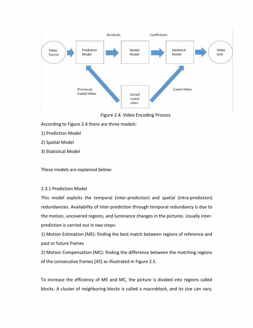
Figure 2.4. Video Encoding Process

According to Figure 2.4 there are three models:

1) Prediction Model

2) Spatial Model

3) Statistical Model

These models are explained below:

2.3.1 Prediction Model

This model exploits the temporal (inter-prediction) and spatial (intra-prediction)

redundancies. Availability of inter-prediction through temporal redundancy is due to

the motion, uncovered regions, and luminance changes in the pictures. Usually inter-

prediction is carried out in two steps:

1) Motion Estimation (ME): finding the best match between regions of reference and

past or future frames

2) Motion Compensation (MC): finding the difference between the matching regions

of the consecutive frames [45] as illustrated in Figure 2.5.

To increase the efficiency of ME and MC, the picture is divided into regions called

blocks. A cluster of neighboring blocks is called a macroblock, and its size can vary.

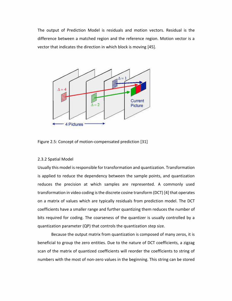
The output of Prediction Model is residuals and motion vectors. Residual is the

difference between a matched region and the reference region. Motion vector is a

vector that indicates the direction in which block is moving [45].

Figure 2.5: Concept of motion-compensated prediction [31]

2.3.2 Spatial Model

Usually this model is responsible for transformation and quantization. Transformation

is applied to reduce the dependency between the sample points, and quantization

reduces the precision at which samples are represented. A commonly used

transformation in video coding is the discrete cosine transform (DCT) [4] that operates

on a matrix of values which are typically residuals from prediction model. The DCT

coefficients have a smaller range and further quantizing them reduces the number of

bits required for coding. The coarseness of the quantizer is usually controlled by a

quantization parameter (QP) that controls the quantization step size.

Because the output matrix from quantization is composed of many zeros, it is

beneficial to group the zero entities. Due to the nature of DCT coefficients, a zigzag

scan of the matrix of quantized coefficients will reorder the coefficients to string of

numbers with the most of non-zero values in the beginning. This string can be stored

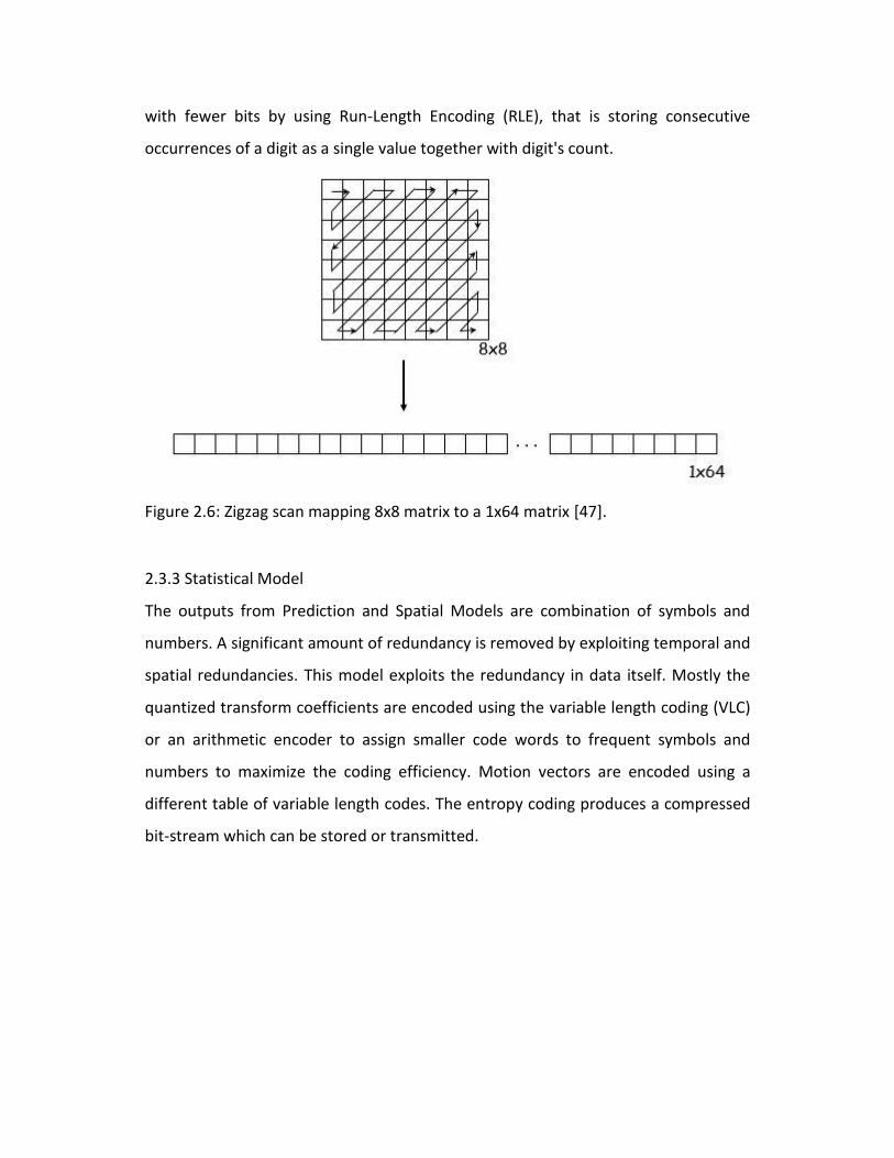
with fewer bits by using Run-Length Encoding (RLE), that is storing consecutive

occurrences of a digit as a single value together with digit's count.

Figure 2.6: Zigzag scan mapping 8x8 matrix to a 1x64 matrix [47].

2.3.3 Statistical Model

The outputs from Prediction and Spatial Models are combination of symbols and

numbers. A significant amount of redundancy is removed by exploiting temporal and

spatial redundancies. This model exploits the redundancy in data itself. Mostly the

quantized transform coefficients are encoded using the variable length coding (VLC)

or an arithmetic encoder to assign smaller code words to frequent symbols and

numbers to maximize the coding efficiency. Motion vectors are encoded using a

different table of variable length codes. The entropy coding produces a compressed

bit-stream which can be stored or transmitted.

2.4 Video Quality Measurement

The best method of evaluating the visual quality of an image or video sequence is

through subjective evaluation, since usually the goal of encoding the content is to be

seen by end users. However, in practice, subjective evaluation is too inconvenient,

time consuming and expensive. Therefore, several objective metrics have been

proposed to perceive quality of an image or a video sequence. In this thesis three

metrics are used: Peak Signal-to-Noise Ratio (PSNR), Bit-rate (R) and Bit rate Ratio (r)

which are discussed in following sections.

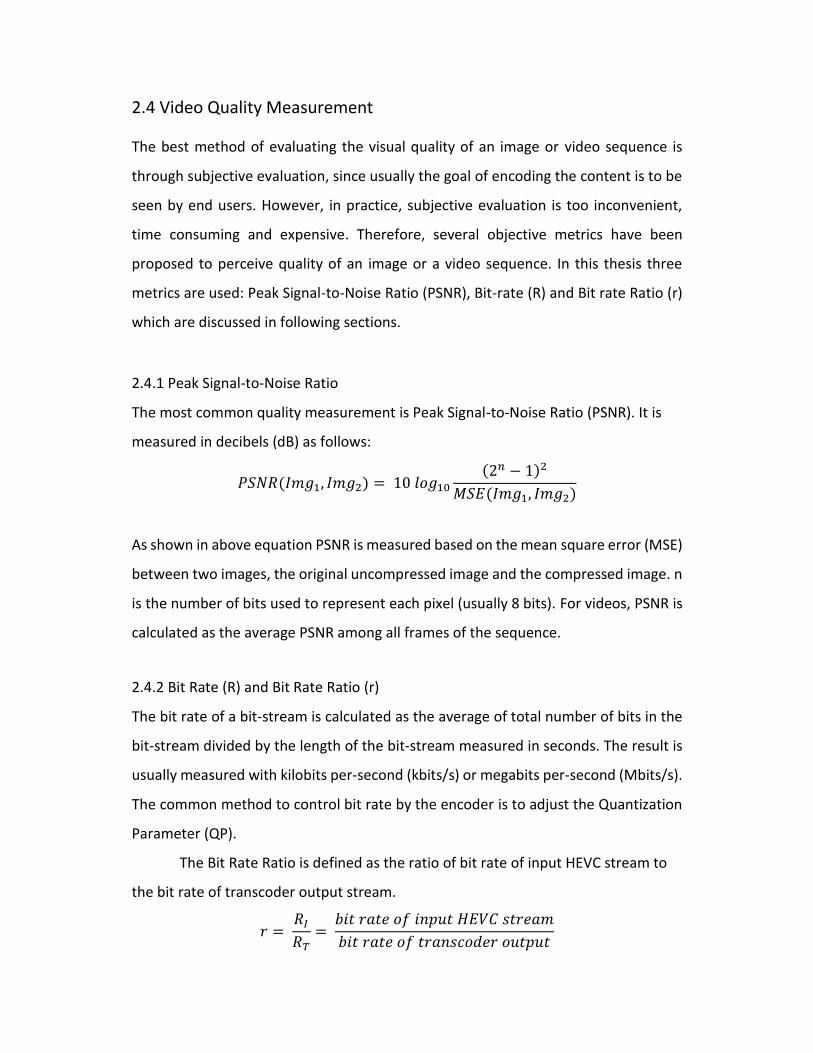
2.4.1 Peak Signal-to-Noise Ratio

The most common quality measurement is Peak Signal-to-Noise Ratio (PSNR). It is

measured in decibels (dB) as follows:

𝑃𝑆𝑁𝑅(𝐼𝑚𝑔1, 𝐼𝑚𝑔2) = 10 𝑙𝑜𝑔10

(2𝑛 − 1)2

𝑀𝑆𝐸(𝐼𝑚𝑔1, 𝐼𝑚𝑔2)

As shown in above equation PSNR is measured based on the mean square error (MSE)

between two images, the original uncompressed image and the compressed image. n

is the number of bits used to represent each pixel (usually 8 bits). For videos, PSNR is

calculated as the average PSNR among all frames of the sequence.

2.4.2 Bit Rate (R) and Bit Rate Ratio (r)

The bit rate of a bit-stream is calculated as the average of total number of bits in the

bit-stream divided by the length of the bit-stream measured in seconds. The result is

usually measured with kilobits per-second (kbits/s) or megabits per-second (Mbits/s).

The common method to control bit rate by the encoder is to adjust the Quantization

Parameter (QP).

The Bit Rate Ratio is defined as the ratio of bit rate of input HEVC stream to

the bit rate of transcoder output stream.

𝑟 = 𝑅𝐼

𝑅𝑇=

𝑏𝑖𝑡 𝑟𝑎𝑡𝑒 𝑜𝑓 𝑖𝑛𝑝𝑢𝑡 𝐻𝐸𝑉𝐶 𝑠𝑡𝑟𝑒𝑎𝑚

𝑏𝑖𝑡 𝑟𝑎𝑡𝑒 𝑜𝑓 𝑡𝑟𝑎𝑛𝑠𝑐𝑜𝑑𝑒𝑟 𝑜𝑢𝑡𝑝𝑢𝑡

3. Overview of High Efficiency Video Coding

3.1 Introduction

High Efficiency Video Coding (HEVC) is the latest global standard on video coding. It

was developed by the Joint Collaborative Team on Video Coding (JCT-VC) and was

standardized in 2013 [1]. HEVC was designed to double the compression ratios of its

predecessor H.264/AVC with a higher computational complexity. After several years

of developments, mature encoding and decoding, solutions are emerging accelerating

the upgrade of the video coding standards of video contents from the legacy

standards such as H.264/AVC [28]. With the increasing needs of ultra-high resolution

videos, it can be foreseen that HEVC will become the most important video coding

standard soon.

Video coding standards have evolved primarily through the development of

the well-known ITU-T and ISO/IEC standards. The ITU-T developed H.261 [5] and

H.263 [6], ISO/IEC developed MPEG-1 [7] and MPEG-4 Visual [8], and the two

organizations jointly developed the H.262/MPEG-2 Video [9] and H.264/MPEG-4

Advanced Video Coding (AVC) [10] standards. The two standards that were jointly

developed have had a particularly strong impact and have found their way into a wide

variety of products that are increasingly prevalent in our daily lives. Throughout this

evolution, continuous efforts have been made to maximize compression capability

and improve data loss robustness, while considering the computational complexity

that were practical for use in products at the time of anticipated deployment of each

standard. The major video coding standard directly preceding the HEVC project is

H.264/MPEG-4 AVC [11]. This was initially developed in the period between 1999 and

2003, and then was extended in several important ways from 2003–2009.

H.264/MPEG-4 AVC has been an enabling technology for digital video in almost every

area that was not previously covered by H.262/MPEG-2 [9] video and has substantially

displaced the older standard within its existing application domains. It is widely used

for many applications, including broadcast of high definition (HD) TV signals over

satellite, cable, and terrestrial transmission systems, video content acquisition and

editing systems, camcorders, security applications, Internet and mobile network

video, Blu-ray Discs, and real-time conversational applications such as video chat,

video conferencing, and telepresence systems.

However, an increasing diversity of services, the growing popularity of HD

video, and the emergence of beyond- HD formats (e.g., 4k × 2k or 8k × 4k resolution),

higher frame rates, higher dynamic range (HDR) are creating even stronger needs for

coding efficiency superior to H.264/ MPEG-4 AVC’s capabilities. The need is even

stronger when higher resolution is accompanied by stereo or multi view capture and

display. Moreover, the traffic caused by video applications targeting mobile devices

and tablets PCs, as well as the transmission needs for video-on-demand (VOD)

services, are imposing severe challenges on today’s networks. An increased desire for

higher quality and resolutions is also arising in mobile applications [11].

HEVC has been designed to address essentially all the existing applications of

H.264/MPEG-4 AVC and to particularly focus on two key issues: increased video

resolution and increased use of parallel processing architectures [23].

3.2 Profiles and Levels

Profiles and levels specify conformance points for implementing the standard in an

interoperable way across various applications that have similar functional

requirements. A profile defines a set of coding tools or algorithms that can be used

in generating a conforming bit stream, whereas a level places constraints on certain

key parameters of the bit stream, corresponding to decoder processing load and

memory capabilities. Figure 3.1, lists the spatial resolutions ranging from SD (NTSC) to

super Hi-Vision/ultra HD video.

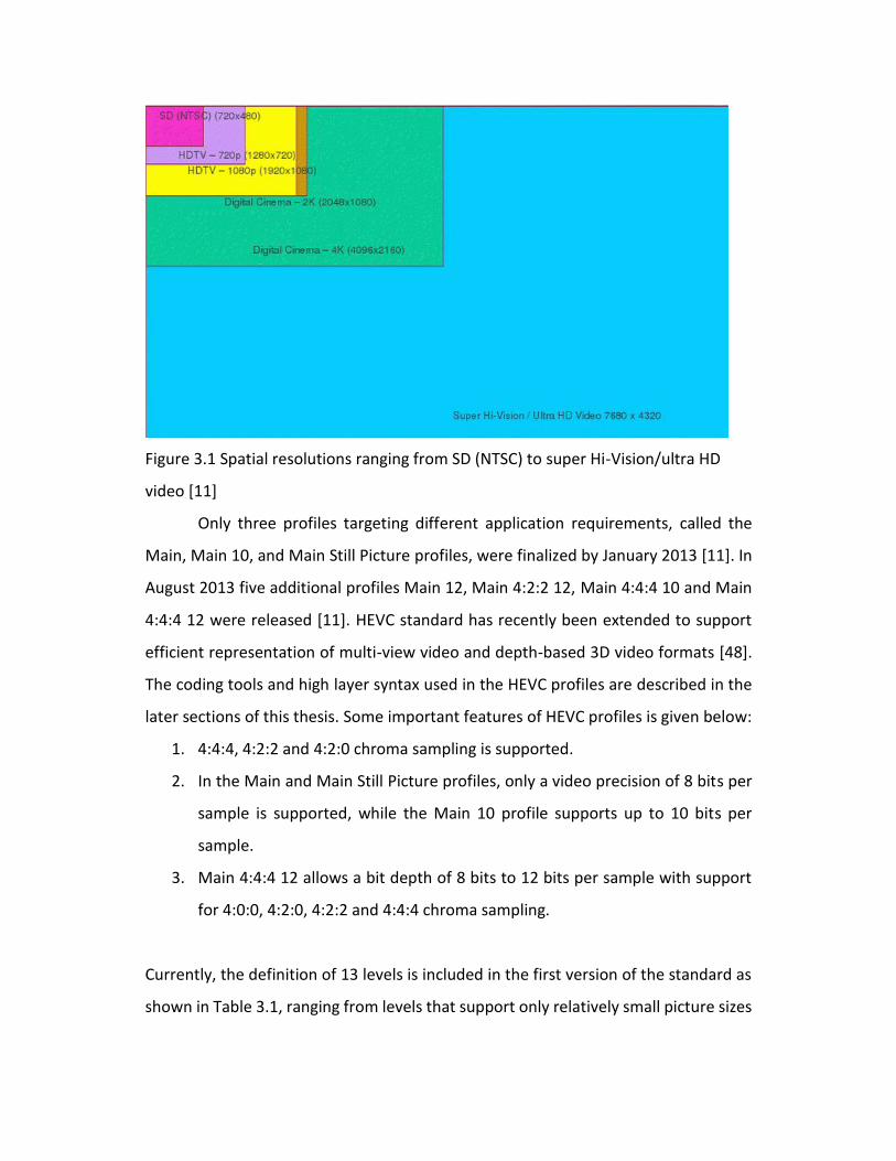
Figure 3.1 Spatial resolutions ranging from SD (NTSC) to super Hi-Vision/ultra HD

video [11]

Only three profiles targeting different application requirements, called the

Main, Main 10, and Main Still Picture profiles, were finalized by January 2013 [11]. In

August 2013 five additional profiles Main 12, Main 4:2:2 12, Main 4:4:4 10 and Main

4:4:4 12 were released [11]. HEVC standard has recently been extended to support

efficient representation of multi-view video and depth-based 3D video formats [48].

The coding tools and high layer syntax used in the HEVC profiles are described in the

later sections of this thesis. Some important features of HEVC profiles is given below:

1. 4:4:4, 4:2:2 and 4:2:0 chroma sampling is supported.

2. In the Main and Main Still Picture profiles, only a video precision of 8 bits per

sample is supported, while the Main 10 profile supports up to 10 bits per

sample.

3. Main 4:4:4 12 allows a bit depth of 8 bits to 12 bits per sample with support

for 4:0:0, 4:2:0, 4:2:2 and 4:4:4 chroma sampling.

Currently, the definition of 13 levels is included in the first version of the standard as

shown in Table 3.1, ranging from levels that support only relatively small picture sizes

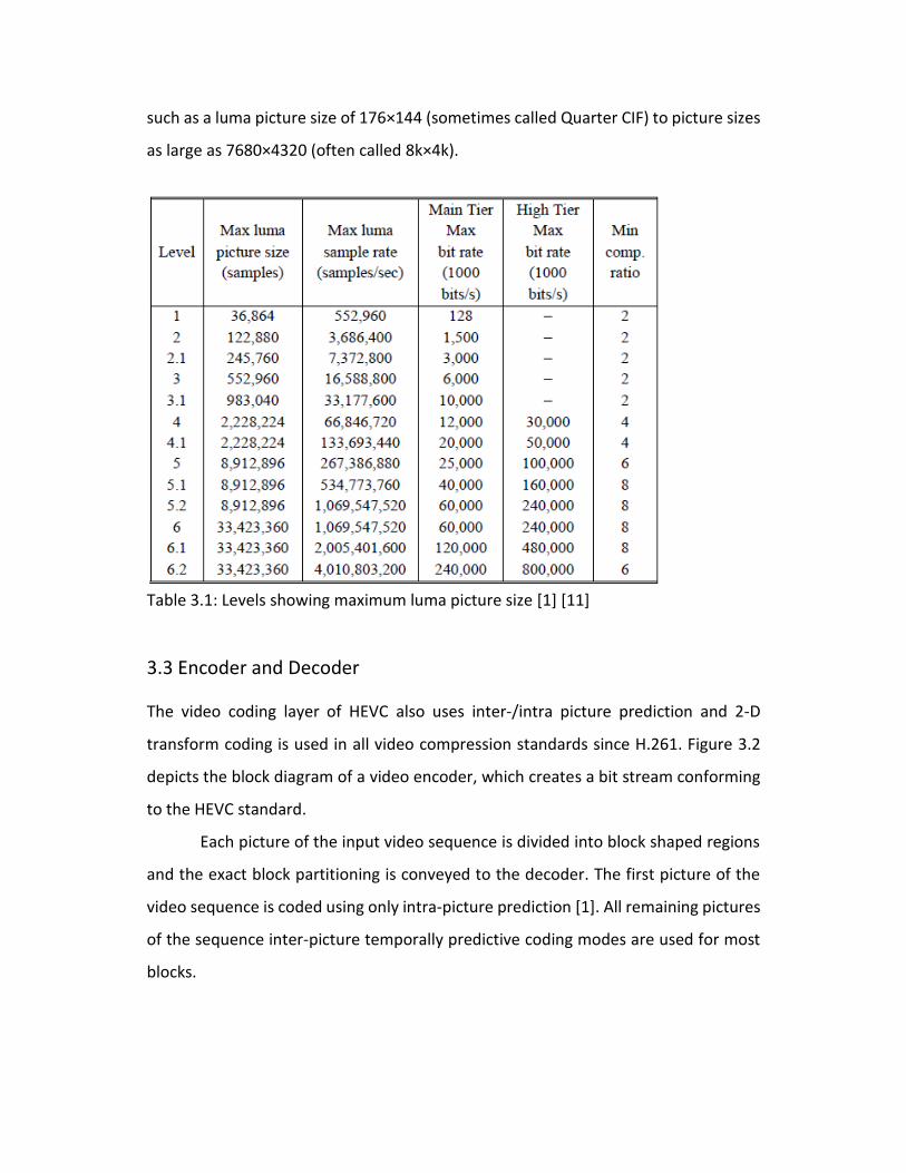
such as a luma picture size of 176×144 (sometimes called Quarter CIF) to picture sizes

as large as 7680×4320 (often called 8k×4k).

Table 3.1: Levels showing maximum luma picture size [1] [11]

3.3 Encoder and Decoder

The video coding layer of HEVC also uses inter-/intra picture prediction and 2-D

transform coding is used in all video compression standards since H.261. Figure 3.2

depicts the block diagram of a video encoder, which creates a bit stream conforming

to the HEVC standard.

Each picture of the input video sequence is divided into block shaped regions

and the exact block partitioning is conveyed to the decoder. The first picture of the

video sequence is coded using only intra-picture prediction [1]. All remaining pictures

of the sequence inter-picture temporally predictive coding modes are used for most

blocks.

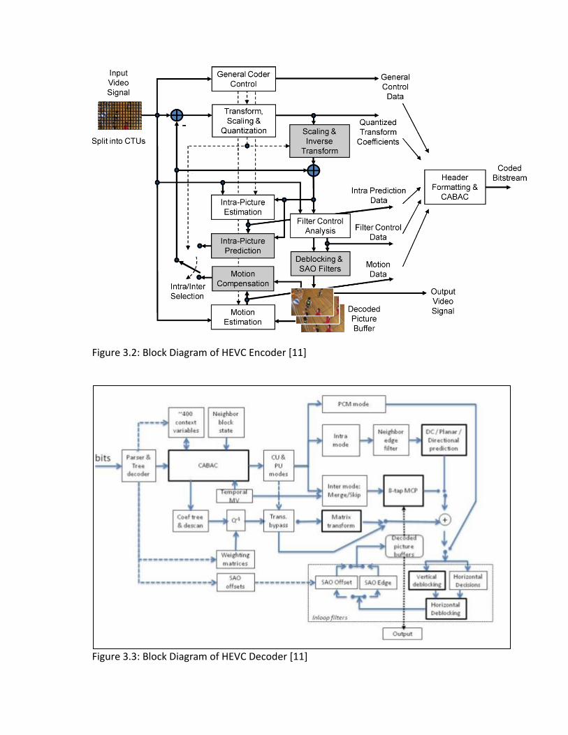
Figure 3.2: Block Diagram of HEVC Encoder [11]

Figure 3.3: Block Diagram of HEVC Decoder [11]

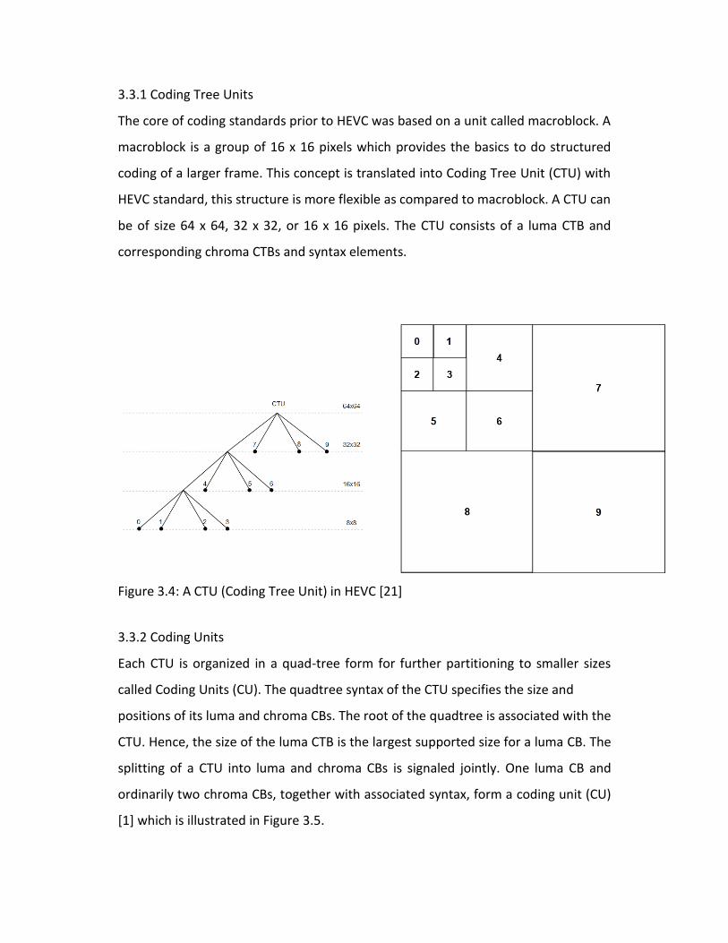
3.3.1 Coding Tree Units

The core of coding standards prior to HEVC was based on a unit called macroblock. A

macroblock is a group of 16 x 16 pixels which provides the basics to do structured

coding of a larger frame. This concept is translated into Coding Tree Unit (CTU) with

HEVC standard, this structure is more flexible as compared to macroblock. A CTU can

be of size 64 x 64, 32 x 32, or 16 x 16 pixels. The CTU consists of a luma CTB and

corresponding chroma CTBs and syntax elements.

Figure 3.4: A CTU (Coding Tree Unit) in HEVC [21]

3.3.2 Coding Units

Each CTU is organized in a quad-tree form for further partitioning to smaller sizes

called Coding Units (CU). The quadtree syntax of the CTU specifies the size and

positions of its luma and chroma CBs. The root of the quadtree is associated with the

CTU. Hence, the size of the luma CTB is the largest supported size for a luma CB. The

splitting of a CTU into luma and chroma CBs is signaled jointly. One luma CB and

ordinarily two chroma CBs, together with associated syntax, form a coding unit (CU)

[1] which is illustrated in Figure 3.5.

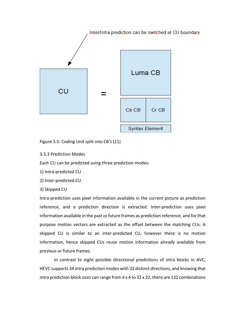
Figure 3.5: Coding Unit split into CB’s [11]

3.3.3 Prediction Modes

Each CU can be predicted using three prediction modes:

1) Intra-predicted CU

2) Inter-predicted CU

3) Skipped CU

Intra-prediction uses pixel information available in the current picture as prediction

reference, and a prediction direction is extracted. Inter-prediction uses pixel

information available in the past or future frames as prediction reference, and for that

purpose motion vectors are extracted as the offset between the matching CUs. A

skipped CU is similar to an inter-predicted CU, however there is no motion

information, hence skipped CUs reuse motion information already available from

previous or future frames.

In contrast to eight possible directional predictions of intra blocks in AVC,

HEVC supports 34 intra prediction modes with 33 distinct directions, and knowing that

intra prediction block sizes can range from 4 x 4 to 32 x 32, there are 132 combinations

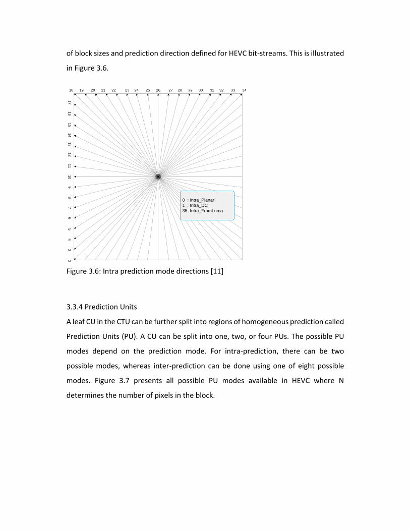
of block sizes and prediction direction defined for HEVC bit-streams. This is illustrated

in Figure 3.6.

17

16

15

14

13

12

11

10

9 8

7 6

5 4

3 2

18 19 20 21 22 23 24 25 26 27 28 29 30 31 32 33 34

0 : Intra_Planar

1 : Intra_DC

35: Intra_FromLuma

Figure 3.6: Intra prediction mode directions [11]

3.3.4 Prediction Units

A leaf CU in the CTU can be further split into regions of homogeneous prediction called

Prediction Units (PU). A CU can be split into one, two, or four PUs. The possible PU

modes depend on the prediction mode. For intra-prediction, there can be two

possible modes, whereas inter-prediction can be done using one of eight possible

modes. Figure 3.7 presents all possible PU modes available in HEVC where N

determines the number of pixels in the block.

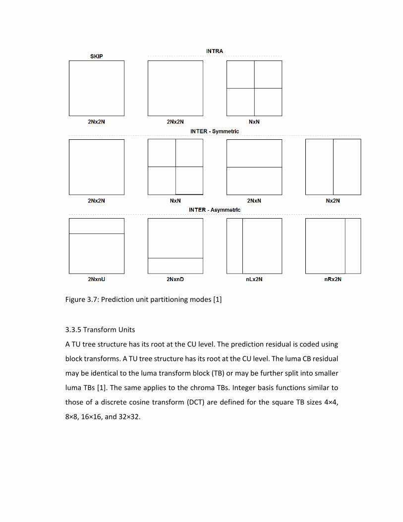
Figure 3.7: Prediction unit partitioning modes [1]

3.3.5 Transform Units

A TU tree structure has its root at the CU level. The prediction residual is coded using

block transforms. A TU tree structure has its root at the CU level. The luma CB residual

may be identical to the luma transform block (TB) or may be further split into smaller

luma TBs [1]. The same applies to the chroma TBs. Integer basis functions similar to

those of a discrete cosine transform (DCT) are defined for the square TB sizes 4×4,

8×8, 16×16, and 32×32.

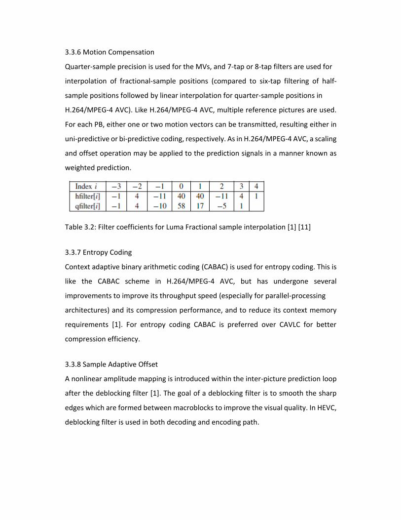
3.3.6 Motion Compensation

Quarter-sample precision is used for the MVs, and 7-tap or 8-tap filters are used for

interpolation of fractional-sample positions (compared to six-tap filtering of half-

sample positions followed by linear interpolation for quarter-sample positions in

H.264/MPEG-4 AVC). Like H.264/MPEG-4 AVC, multiple reference pictures are used.

For each PB, either one or two motion vectors can be transmitted, resulting either in

uni-predictive or bi-predictive coding, respectively. As in H.264/MPEG-4 AVC, a scaling

and offset operation may be applied to the prediction signals in a manner known as

weighted prediction.

Table 3.2: Filter coefficients for Luma Fractional sample interpolation [1] [11]

3.3.7 Entropy Coding

Context adaptive binary arithmetic coding (CABAC) is used for entropy coding. This is

like the CABAC scheme in H.264/MPEG-4 AVC, but has undergone several

improvements to improve its throughput speed (especially for parallel-processing

architectures) and its compression performance, and to reduce its context memory

requirements [1]. For entropy coding CABAC is preferred over CAVLC for better

compression efficiency.

3.3.8 Sample Adaptive Offset

A nonlinear amplitude mapping is introduced within the inter-picture prediction loop

after the deblocking filter [1]. The goal of a deblocking filter is to smooth the sharp

edges which are formed between macroblocks to improve the visual quality. In HEVC,

deblocking filter is used in both decoding and encoding path.

3.4 Summary

This chapter describes the overview of HEVC, Profiles and levels along with some key

features of HEVC coding design. Next chapter describes the need for transcoding,

various transcoding architectures and the proposed homogeneous transcoder.

4. Transcoding

4.1 Introduction

Video transcoding can change the video format or change video characteristics such

as resolution or bit rate. The focus of this thesis is on transcoding for bit rate

reduction. Transcoding is the process that converts from one compressed bit stream

(called the source or incoming bit stream) to another compressed bit stream (called

the target or transcoded bit stream) [2, 12, 13]. Several properties may change during

transcoding: the video format [34, 35], the bitrate of the video [36, 37], the frame

rate, the spatial resolution [38] etc.

4.2 Need for Transcoding There are also several possible application scenarios for transcoding. One example is

to deliver a high-quality video content through a more restricted wireless network to

be accessed by mobile phones. In this case, the spatial and temporal resolutions may

have to be reduced to fit the device playing capabilities and the bitrate may have to

be reduced to suit the network bandwidth. Another example is to broadcast a video

content compressed in H.265/HEVC format through a digital television system that

uses H.264 as the video format. In this case, even though the compression

performance of H.265/HEVC is higher than that of H.264/AVS, the video must be

transcoded to enable communication.

What is common among the application scenario of transcoding is that one or

more characteristics of the video bit stream need to change to allow communication

between the two systems [12]. To allow the inter-operation of multimedia content,

transcoding is needed both within and across different formats.

4.3 Video Transcoding Challenges

Transcoding can have two main issues: transcoding can increase distortion and

complexity [39]. Distortion, in the context of video coding, is the picture quality at a

given bit rate. Complexity refers to processing time and memory requirements.

4.3.1 Distortion Transcoded video sequence is created by decoding and re-encoding the input bit

stream. The transcoded bit stream has lower bit rate which increases distortion in

the frames. The goal of this thesis is to reduce bit rate and provide a transcoded bit

stream having lower distortion. Transcoding of a video sequence that has degraded

input video quality will further reduce its quality.

4.3.2 Computational Complexity When constrained by resources, time complexity introduces delay, and memory

complexity limits the maximum quality. In some applications, such as real-time video

broadcasting, time complexity of transcoding is important and it is required to be

minimized.

4.4 Video Transcoding Methods

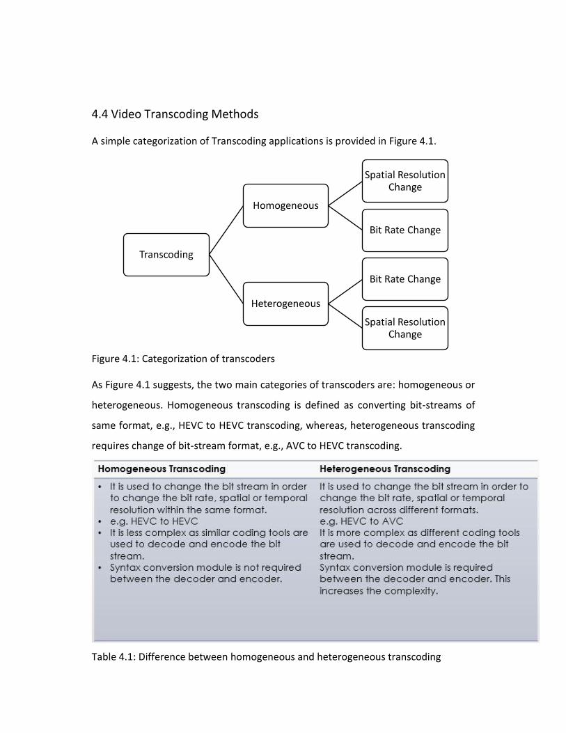
A simple categorization of Transcoding applications is provided in Figure 4.1.

Figure 4.1: Categorization of transcoders

As Figure 4.1 suggests, the two main categories of transcoders are: homogeneous or

heterogeneous. Homogeneous transcoding is defined as converting bit-streams of

same format, e.g., HEVC to HEVC transcoding, whereas, heterogeneous transcoding

requires change of bit-stream format, e.g., AVC to HEVC transcoding.

Table 4.1: Difference between homogeneous and heterogeneous transcoding

Transcoding

Homogeneous

Spatial Resolution Change

Bit Rate Change

Heterogeneous

Bit Rate Change

Spatial Resolution Change

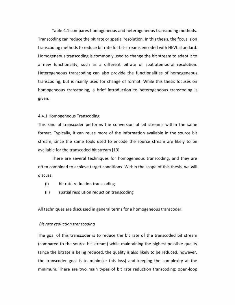
Table 4.1 compares homogeneous and heterogeneous transcoding methods.

Transcoding can reduce the bit rate or spatial resolution. In this thesis, the focus is on

transcoding methods to reduce bit rate for bit-streams encoded with HEVC standard.

Homogeneous transcoding is commonly used to change the bit stream to adapt it to

a new functionality, such as a different bitrate or spatiotemporal resolution.

Heterogeneous transcoding can also provide the functionalities of homogeneous

transcoding, but is mainly used for change of format. While this thesis focuses on

homogeneous transcoding, a brief introduction to heterogeneous transcoding is

given.

4.4.1 Homogeneous Transcoding

This kind of transcoder performs the conversion of bit streams within the same

format. Typically, it can reuse more of the information available in the source bit

stream, since the same tools used to encode the source stream are likely to be

available for the transcoded bit stream [13].

There are several techniques for homogeneous transcoding, and they are

often combined to achieve target conditions. Within the scope of this thesis, we will

discuss:

(i) bit rate reduction transcoding

(ii) spatial resolution reduction transcoding

All techniques are discussed in general terms for a homogeneous transcoder.

Bit rate reduction transcoding The goal of this transcoder is to reduce the bit rate of the transcoded bit stream

(compared to the source bit stream) while maintaining the highest possible quality

(since the bitrate is being reduced, the quality is also likely to be reduced, however,

the transcoder goal is to minimize this loss) and keeping the complexity at the

minimum. There are two main types of bit rate reduction transcoding: open-loop

system and closed-loop system [13]. The former has the advantage of very low

complexity, but it suffers from degraded quality due to drift, while the latter is more

complex, but yields a better performance.

Spatial resolution reduction transcoding In this type of transcoding, the spatial resolution of the transcoded stream is lower

than the resolution of the source stream. This also produces a bit rate reduction. Some

key techniques are the reuse of data at the macroblock level and mapping the motion

estimation to the new spatial resolution [40]. Downsampling in the DCT domain is also

possible.

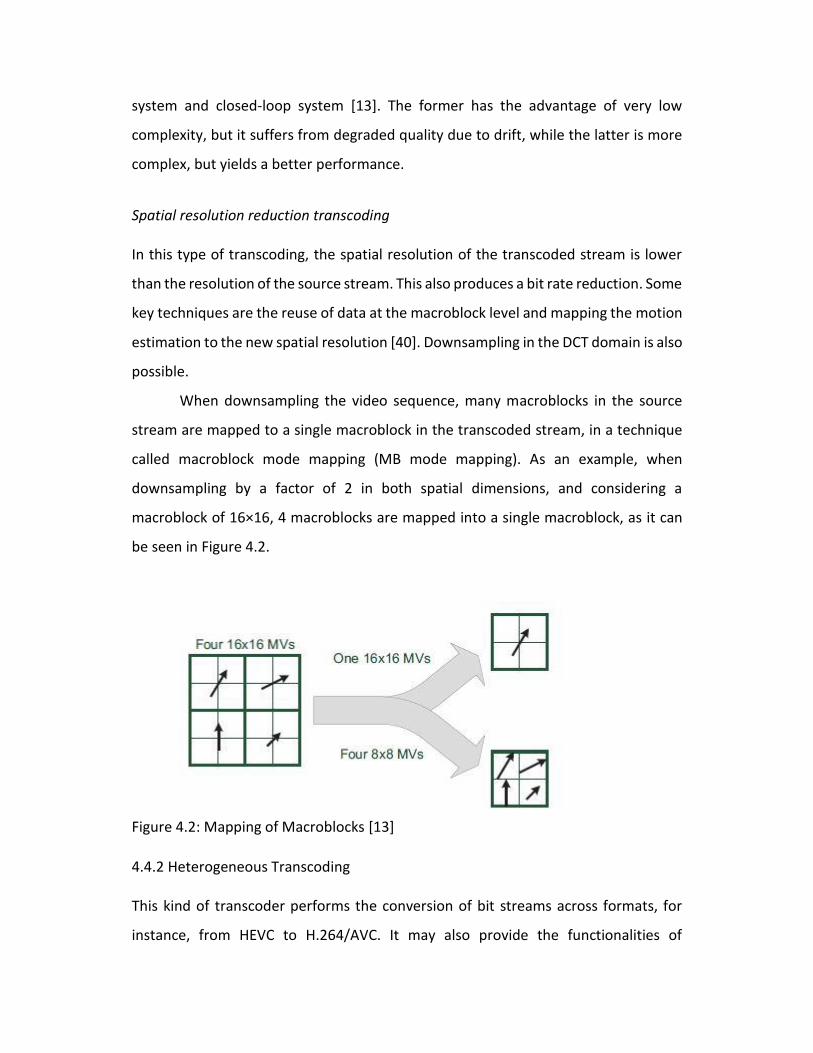
When downsampling the video sequence, many macroblocks in the source

stream are mapped to a single macroblock in the transcoded stream, in a technique

called macroblock mode mapping (MB mode mapping). As an example, when

downsampling by a factor of 2 in both spatial dimensions, and considering a

macroblock of 16×16, 4 macroblocks are mapped into a single macroblock, as it can

be seen in Figure 4.2.

Figure 4.2: Mapping of Macroblocks [13]

4.4.2 Heterogeneous Transcoding This kind of transcoder performs the conversion of bit streams across formats, for

instance, from HEVC to H.264/AVC. It may also provide the functionalities of

homogeneous transcoding, like bit rate reduction and spatial resolution reduction,

and some techniques developed for homogeneous transcoding may also be used

[13, 2].

The biggest difference from the architecture of a homogeneous transcoder to

a heterogeneous transcoder is the presence of a syntax conversion module in the

latter. Also, since the two codecs may use different tools (or may use the same tools

with different settings), the encoder and decoder motion compensation loops in

heterogeneous transcoder are more complex than in homogeneous transcoders [35].

4.5 Transcoding Architecture

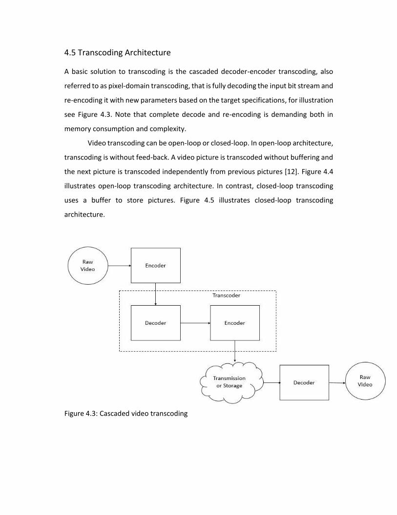
A basic solution to transcoding is the cascaded decoder-encoder transcoding, also

referred to as pixel-domain transcoding, that is fully decoding the input bit stream and

re-encoding it with new parameters based on the target specifications, for illustration

see Figure 4.3. Note that complete decode and re-encoding is demanding both in

memory consumption and complexity.

Video transcoding can be open-loop or closed-loop. In open-loop architecture,

transcoding is without feed-back. A video picture is transcoded without buffering and

the next picture is transcoded independently from previous pictures [12]. Figure 4.4

illustrates open-loop transcoding architecture. In contrast, closed-loop transcoding

uses a buffer to store pictures. Figure 4.5 illustrates closed-loop transcoding

architecture.

Figure 4.3: Cascaded video transcoding

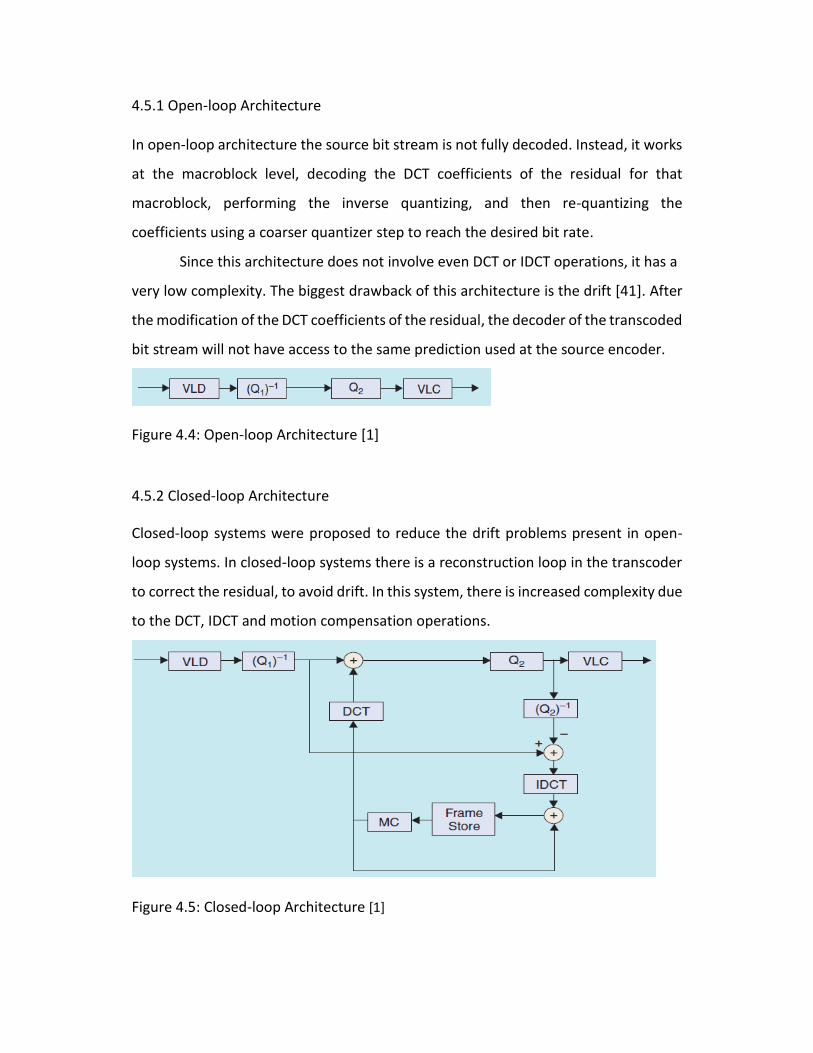
4.5.1 Open-loop Architecture In open-loop architecture the source bit stream is not fully decoded. Instead, it works

at the macroblock level, decoding the DCT coefficients of the residual for that

macroblock, performing the inverse quantizing, and then re-quantizing the

coefficients using a coarser quantizer step to reach the desired bit rate.

Since this architecture does not involve even DCT or IDCT operations, it has a

very low complexity. The biggest drawback of this architecture is the drift [41]. After

the modification of the DCT coefficients of the residual, the decoder of the transcoded

bit stream will not have access to the same prediction used at the source encoder.

Figure 4.4: Open-loop Architecture [1]

4.5.2 Closed-loop Architecture

Closed-loop systems were proposed to reduce the drift problems present in open-

loop systems. In closed-loop systems there is a reconstruction loop in the transcoder

to correct the residual, to avoid drift. In this system, there is increased complexity due

to the DCT, IDCT and motion compensation operations.

Figure 4.5: Closed-loop Architecture [1]

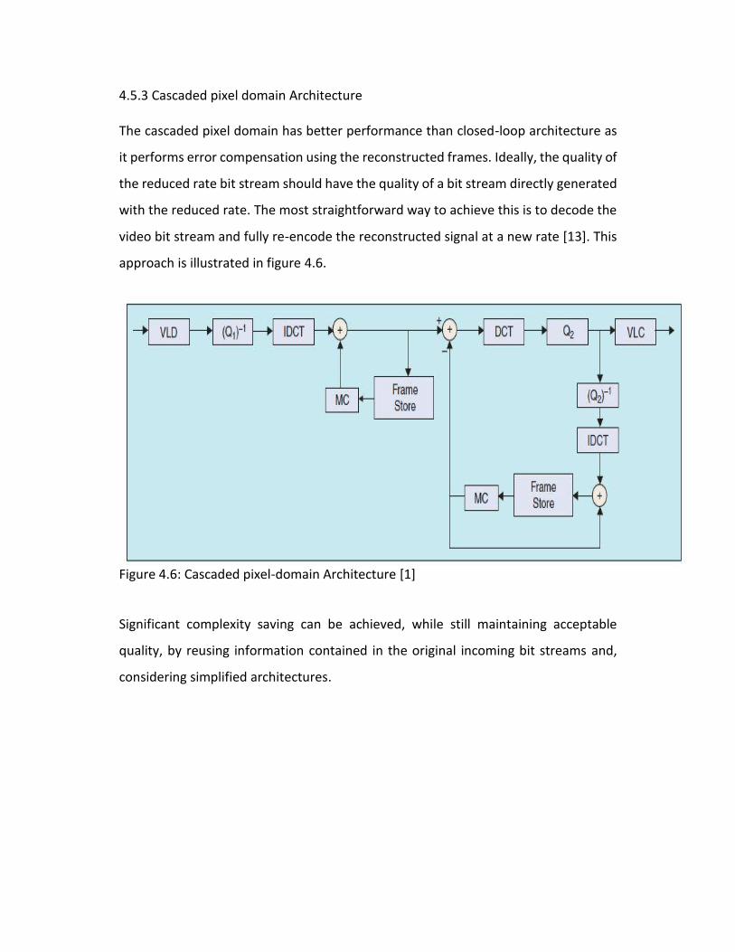
4.5.3 Cascaded pixel domain Architecture The cascaded pixel domain has better performance than closed-loop architecture as

it performs error compensation using the reconstructed frames. Ideally, the quality of

the reduced rate bit stream should have the quality of a bit stream directly generated

with the reduced rate. The most straightforward way to achieve this is to decode the

video bit stream and fully re-encode the reconstructed signal at a new rate [13]. This

approach is illustrated in figure 4.6.

Figure 4.6: Cascaded pixel-domain Architecture [1]

Significant complexity saving can be achieved, while still maintaining acceptable

quality, by reusing information contained in the original incoming bit streams and,

considering simplified architectures.

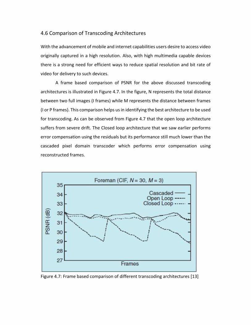
4.6 Comparison of Transcoding Architectures With the advancement of mobile and internet capabilities users desire to access video

originally captured in a high resolution. Also, with high multimedia capable devices

there is a strong need for efficient ways to reduce spatial resolution and bit rate of

video for delivery to such devices.

A frame based comparison of PSNR for the above discussed transcoding

architectures is illustrated in Figure 4.7. In the figure, N represents the total distance

between two full images (I frames) while M represents the distance between frames

(I or P frames). This comparison helps us in identifying the best architecture to be used

for transcoding. As can be observed from Figure 4.7 that the open loop architecture

suffers from severe drift. The Closed loop architecture that we saw earlier performs

error compensation using the residuals but its performance still much lower than the

cascaded pixel domain transcoder which performs error compensation using

reconstructed frames.

Figure 4.7: Frame based comparison of different transcoding architectures [13]

4.7 Related Work

There are quite a few research works on video transcoding between different coding

standards, which is defined as heterogeneous transcoding in [12]. In [13], the authors

discuss some key issues in generic video transcoding process. The authors of [14, 15,

16] provide some thoughts on transcoding among MPEG-2, MPEG-4 and H.264.

After the HEVC standard was finalized, there were more explorations on

transcoding from H.264/AVC to HEVC. Zhang et al [17] proposed a solution where the

number of candidates for the coding unit (CU) and prediction unit (PU) partition sizes

was reduced for the intra-pictures, while for the inter-pictures, a power-spectrum

based rate-distortion optimization model-based power spectrum was used to

estimate the best CU split tree from a reduced set of PU partition candidates

according to the MV information in the input H.264/AVC bit stream. Peixoto et al [18]

proposed a transcoding architecture based on their previous work in [19]. They

proposed two algorithms for mapping modes from H.264/AVC to HEVC, namely,

dynamic thresholding of a single H.264/AVC coding parameter and context modeling

using linear discriminant functions to determine the outgoing HEVC partitions. The

model parameters for the two algorithms were computed using the beginning frames

of a sequence. They achieved a 2.5% – 3.0% speed gain with a BD-rate [20] loss

between 2.95% and 4.42% by the proposed method. Diaz-Honrubia et al [21]

proposed an H.264/AVC to HEVC transcoder based on a statistical NB (Naïve Bayes)

classifier, which decides on the most appropriate quadtree level in the HEVC encoding

process. Their algorithms achieved a speedup of 2.31% on average with a BD-rate

penalty of 3.4%. Mora et al [22] also proposed an H.264/AVC to HEVC transcoder

based on quadtree limitation, where the fusion map generated by the motion

similarity of decoded H.264/AVC blocks is used to limit the quadtree of HEVC coded

frames. They achieved 63% time saving with only a 1.4% bitrate increase. Hingole

analyzed various transcoding architectures for HEVC to H.264 transcoding and

implemented a cascaded heterogeneous transcoder [23] [32].

Because the standardization process of AVS2 is not completed yet, there is

little research work on this new standard [46]. According to the inheritances between

H.264/AVC and HEVC and between AVS1 and AVS2, works on H.264/AVC to AVS

transcoding can be a reference. Wang et al. [24] proposed a fast transcoding algorithm

from H.264/AVC bit stream to AVS bit stream. They used a QP mapping method and

a reciprocal SAD weighted method on intra mode selection and inter MV estimation.

Their algorithms achieved 50% time saving in intra prediction with ignorable coding

performance loss and 40% time saving in inter prediction with minor coding

performance loss.

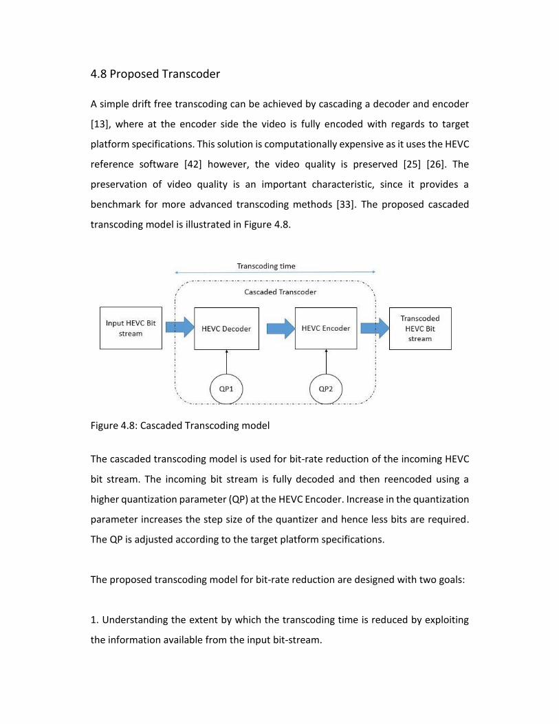
4.8 Proposed Transcoder A simple drift free transcoding can be achieved by cascading a decoder and encoder

[13], where at the encoder side the video is fully encoded with regards to target

platform specifications. This solution is computationally expensive as it uses the HEVC

reference software [42] however, the video quality is preserved [25] [26]. The

preservation of video quality is an important characteristic, since it provides a

benchmark for more advanced transcoding methods [33]. The proposed cascaded

transcoding model is illustrated in Figure 4.8.

Figure 4.8: Cascaded Transcoding model

The cascaded transcoding model is used for bit-rate reduction of the incoming HEVC

bit stream. The incoming bit stream is fully decoded and then reencoded using a

higher quantization parameter (QP) at the HEVC Encoder. Increase in the quantization

parameter increases the step size of the quantizer and hence less bits are required.

The QP is adjusted according to the target platform specifications.

The proposed transcoding model for bit-rate reduction are designed with two goals:

1. Understanding the extent by which the transcoding time is reduced by exploiting

the information available from the input bit-stream.

2. Reducing the bit-rate and producing video quality as close as to the original video

quality.

4.9 Summary Chapter 4 introduces transcoding, describes the two methods of transcoding and

challenges faced while designing a transcoder. It also discusses transcoding

architectures like open-loop, closed-loop and cascaded pixel-domain architectures.

Then, the transcoding architectures are compared as to choose the best transcoding

architecture. In later part of the chapter a detailed description of the proposed

cascaded transcoding architecture is provided. Chapter 5 will show results of

simulations on different test sequences.

5. Results

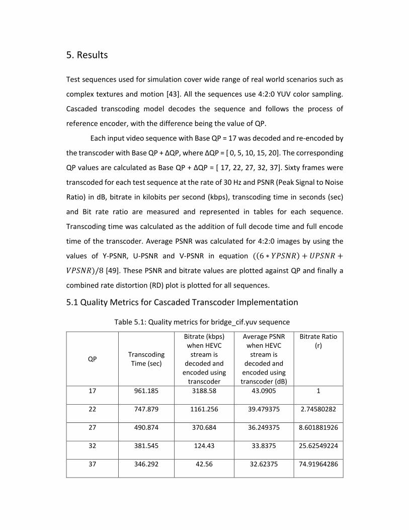
Test sequences used for simulation cover wide range of real world scenarios such as

complex textures and motion [43]. All the sequences use 4:2:0 YUV color sampling.

Cascaded transcoding model decodes the sequence and follows the process of

reference encoder, with the difference being the value of QP.

Each input video sequence with Base QP = 17 was decoded and re-encoded by

the transcoder with Base QP + ΔQP, where ΔQP = [ 0, 5, 10, 15, 20]. The corresponding

QP values are calculated as Base QP + ΔQP = [ 17, 22, 27, 32, 37]. Sixty frames were

transcoded for each test sequence at the rate of 30 Hz and PSNR (Peak Signal to Noise

Ratio) in dB, bitrate in kilobits per second (kbps), transcoding time in seconds (sec)

and Bit rate ratio are measured and represented in tables for each sequence.

Transcoding time was calculated as the addition of full decode time and full encode

time of the transcoder. Average PSNR was calculated for 4:2:0 images by using the

values of Y-PSNR, U-PSNR and V-PSNR in equation ((6 ∗ 𝑌𝑃𝑆𝑁𝑅) + 𝑈𝑃𝑆𝑁𝑅 +

𝑉𝑃𝑆𝑁𝑅)/8 [49]. These PSNR and bitrate values are plotted against QP and finally a

combined rate distortion (RD) plot is plotted for all sequences.

5.1 Quality Metrics for Cascaded Transcoder Implementation

Table 5.1: Quality metrics for bridge_cif.yuv sequence

QP Transcoding Time (sec)

Bitrate (kbps) when HEVC

stream is decoded and

encoded using transcoder

Average PSNR when HEVC


encoded using transcoder (dB)

Bitrate Ratio (r)

17 961.185

3188.58

43.0905

1

22 747.879

1161.256

39.479375

2.74580282

27 490.874

370.684

36.249375

8.601881926

32 381.545

124.43

33.8375

25.62549224

37 346.292

42.56

32.62375

74.91964286

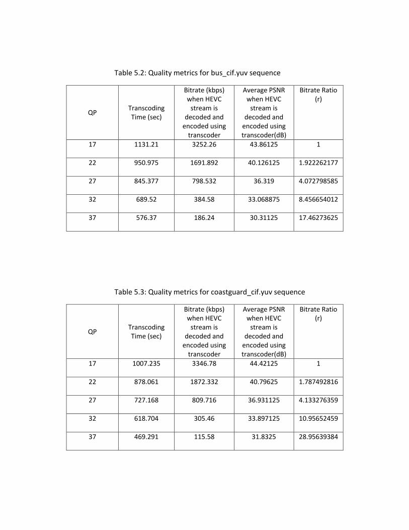
Table 5.2: Quality metrics for bus_cif.yuv sequence







encoded using transcoder(dB)

Bitrate Ratio (r)

17 1131.21

3252.26

43.86125

1

22 950.975

1691.892

40.126125

1.922262177

27 845.377

798.532

36.319

4.072798585

32 689.52

384.58

33.068875

8.456654012

37 576.37

186.24

30.31125

17.46273625

Table 5.3: Quality metrics for coastguard_cif.yuv sequence








Bitrate Ratio (r)

17 1007.235

3346.78

44.42125

1

22 878.061

1872.332

40.79625

1.787492816

27 727.168

809.716

36.931125

4.133276359

32 618.704

305.46

33.897125

10.95652459

37 469.291

115.58

31.8325

28.95639384

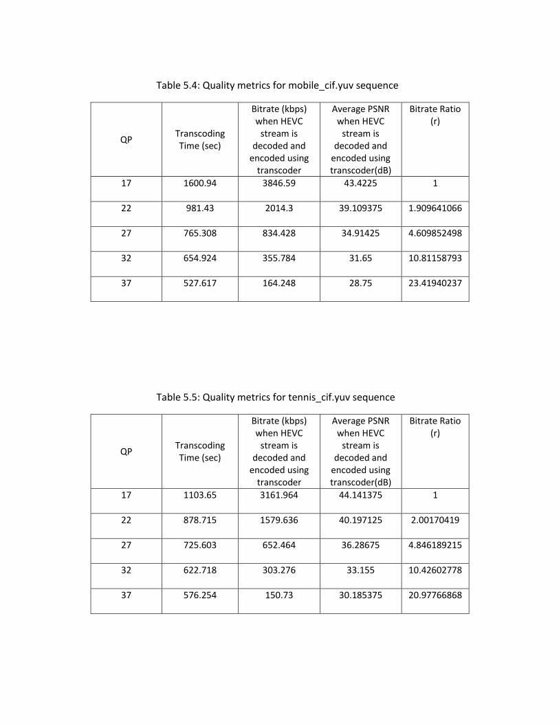
Table 5.4: Quality metrics for mobile_cif.yuv sequence








Bitrate Ratio (r)

17 1600.94

3846.59

43.4225

1

22 981.43

2014.3

39.109375

1.909641066

27 765.308

834.428

34.91425

4.609852498

32 654.924

355.784

31.65

10.81158793

37 527.617

164.248

28.75

23.41940237

Table 5.5: Quality metrics for tennis_cif.yuv sequence








Bitrate Ratio (r)

17 1103.65

3161.964

44.141375

1

22 878.715

1579.636

40.197125

2.00170419

27 725.603

652.464

36.28675

4.846189215

32 622.718

303.276

33.155

10.42602778

37 576.254

150.73

30.185375

20.97766868

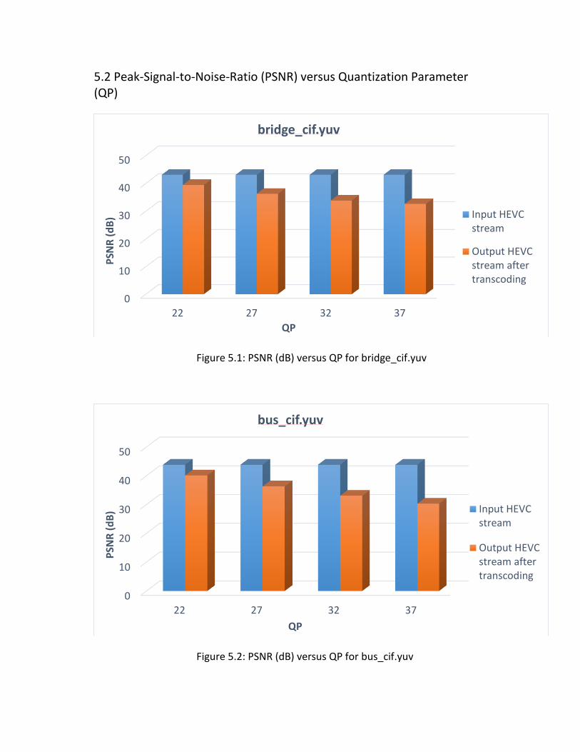
5.2 Peak-Signal-to-Noise-Ratio (PSNR) versus Quantization Parameter (QP)

Figure 5.1: PSNR (dB) versus QP for bridge_cif.yuv

Figure 5.2: PSNR (dB) versus QP for bus_cif.yuv

0

10

20

30

40

50

22 27 32 37

PSN

R (

dB

)

QP

bridge_cif.yuv

Input HEVCstream

Output HEVCstream aftertranscoding

0

10

20

30

40

50

22 27 32 37

PSN

R (

dB

)

QP

bus_cif.yuv

Input HEVCstream


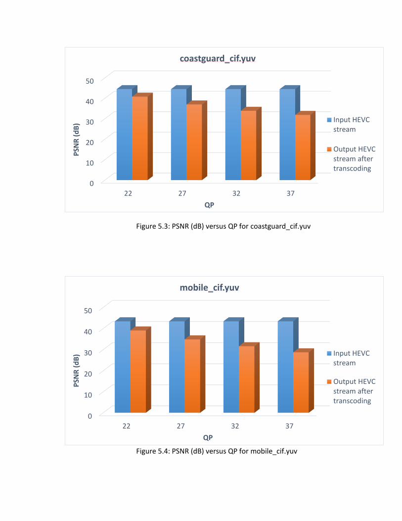
Figure 5.3: PSNR (dB) versus QP for coastguard_cif.yuv

Figure 5.4: PSNR (dB) versus QP for mobile_cif.yuv

0

10

20

30

40

50

22 27 32 37

PSN

R (

dB

)

QP

coastguard_cif.yuv

Input HEVCstream


0

10

20

30

40

50

22 27 32 37

PSN

R (

dB

)

QP

mobile_cif.yuv

Input HEVCstream


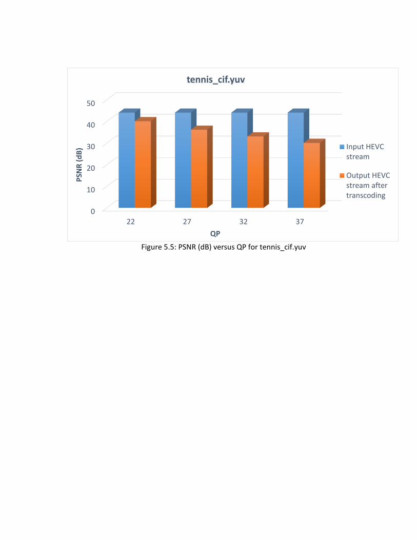
Figure 5.5: PSNR (dB) versus QP for tennis_cif.yuv

0

10

20

30

40

50

22 27 32 37

PSN

R (

dB

)

QP

tennis_cif.yuv

Input HEVCstream


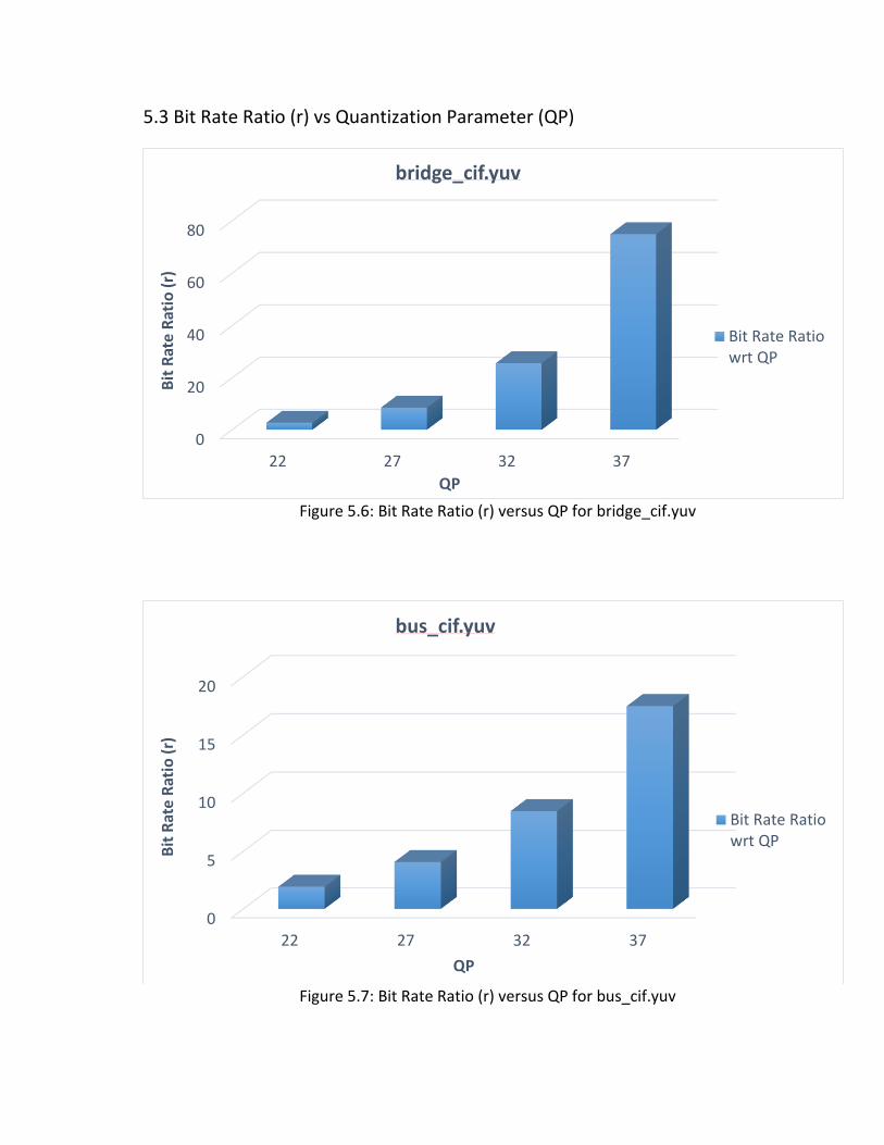
5.3 Bit Rate Ratio (r) vs Quantization Parameter (QP)

Figure 5.6: Bit Rate Ratio (r) versus QP for bridge_cif.yuv

Figure 5.7: Bit Rate Ratio (r) versus QP for bus_cif.yuv

0

20

40

60

80

22 27 32 37

Bit

Rat

e R

atio

(r)

QP

bridge_cif.yuv

Bit Rate Ratiowrt QP

0

5

10

15

20

22 27 32 37

Bit

Rat

e R

atio

(r)

QP

bus_cif.yuv


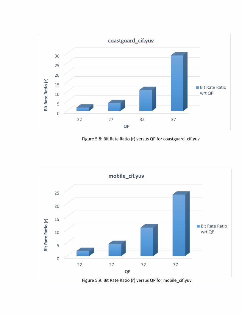
Figure 5.8: Bit Rate Ratio (r) versus QP for coastguard_cif.yuv

Figure 5.9: Bit Rate Ratio (r) versus QP for mobile_cif.yuv

0

5

10

15

20

25

30

22 27 32 37

Bit

Rat

e R

atio

(r)

QP

coastguard_cif.yuv


0

5

10

15

20

25

22 27 32 37

Bit

Rat

e R

atio

(r)

QP

mobile_cif.yuv


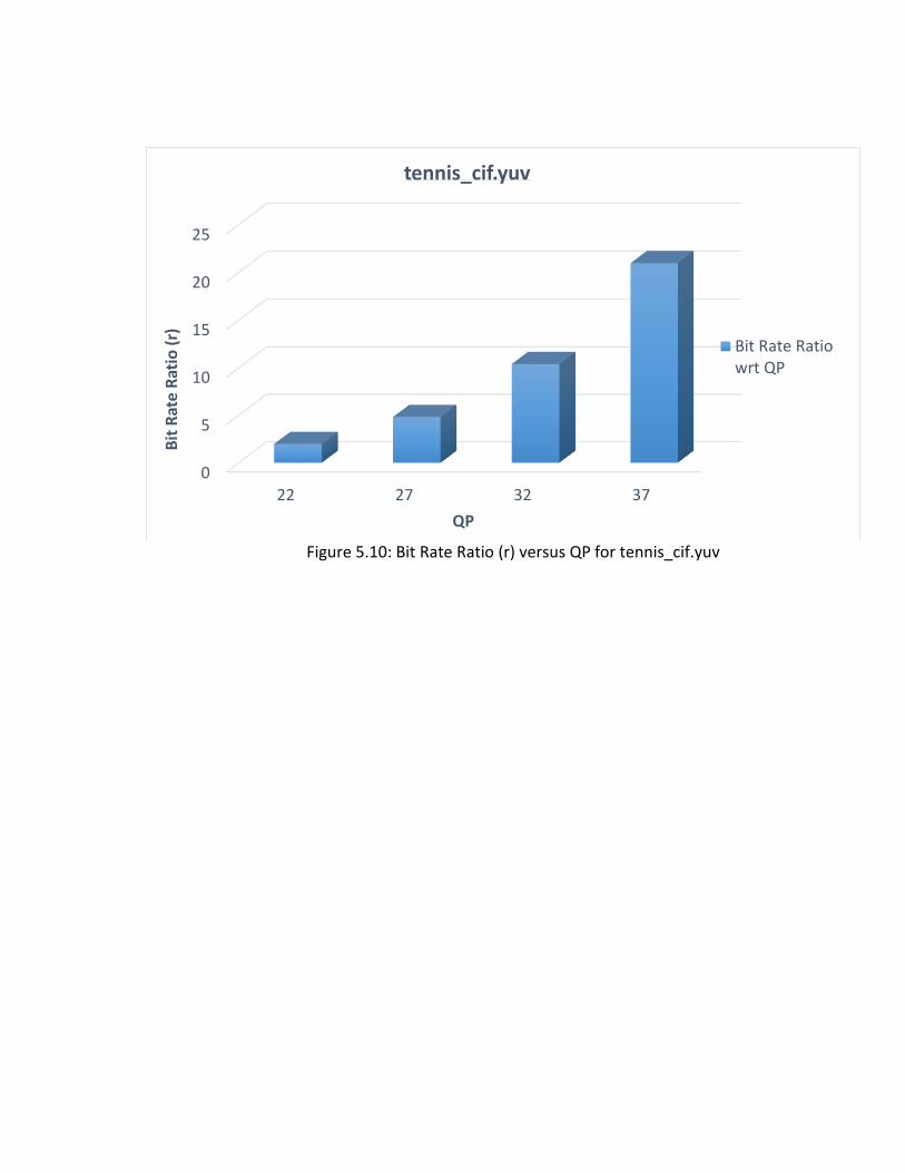
Figure 5.10: Bit Rate Ratio (r) versus QP for tennis_cif.yuv

0

5

10

15

20

25

22 27 32 37

Bit

Rat

e R

atio

(r)

QP

tennis_cif.yuv


5.4 Transcoding Time (sec) vs Quantization Parameter (QP)

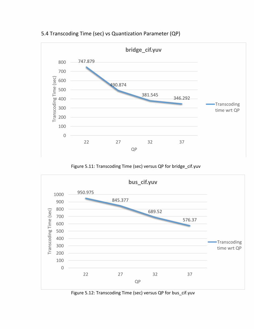
Figure 5.11: Transcoding Time (sec) versus QP for bridge_cif.yuv

Figure 5.12: Transcoding Time (sec) versus QP for bus_cif.yuv

747.879

490.874

381.545346.292

0

100

200

300

400

500

600

700

800

22 27 32 37

Tran

sco

din

g Ti

me

(sec

)

QP

bridge_cif.yuv

Transcodingtime wrt QP

950.975

845.377

689.52

576.37

0

100

200

300

400

500

600

700

800

900

1000

22 27 32 37

Tran

sco

din

g Ti

me

(sec

)

QP

bus_cif.yuv


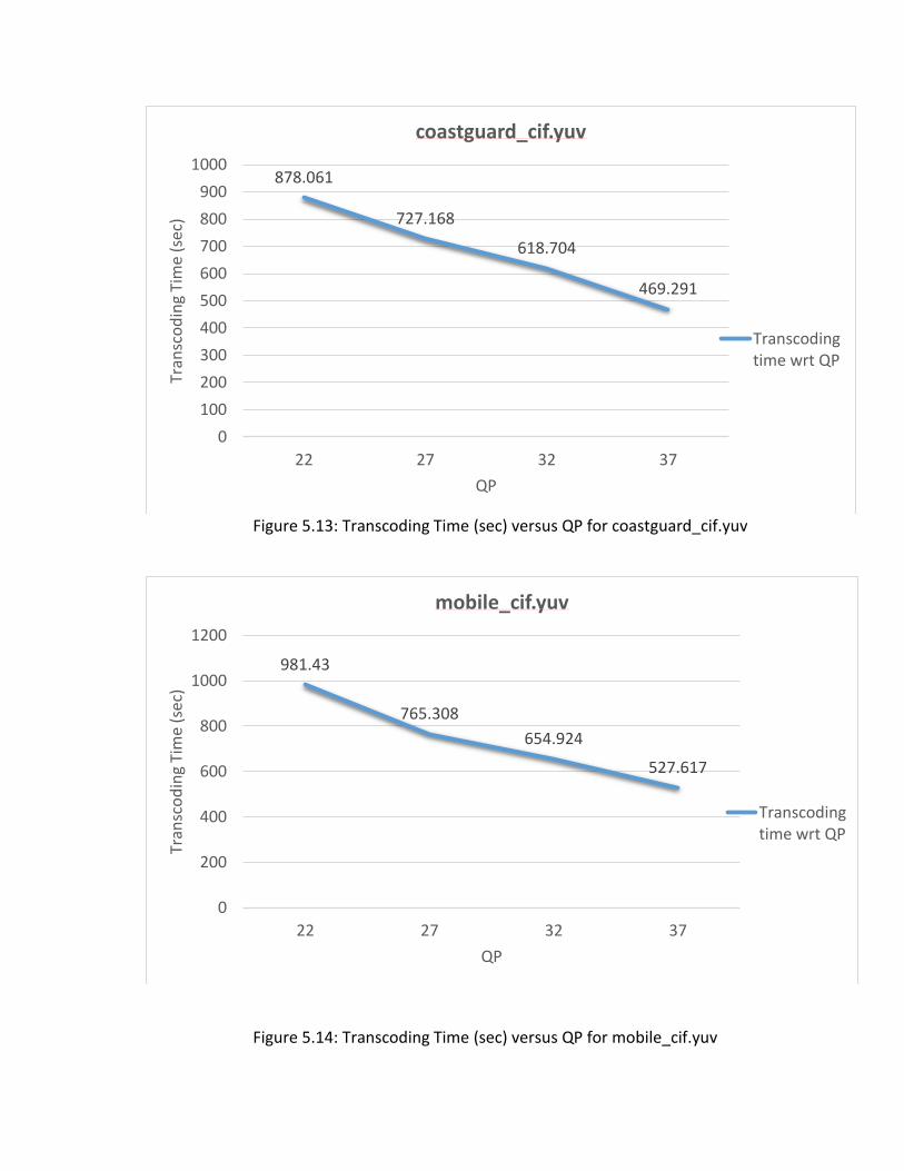
Figure 5.13: Transcoding Time (sec) versus QP for coastguard_cif.yuv

Figure 5.14: Transcoding Time (sec) versus QP for mobile_cif.yuv

878.061

727.168

618.704

469.291

0

100

200

300

400

500

600

700

800

900

1000

22 27 32 37

Tran

sco

din

g Ti

me

(sec

)

QP

coastguard_cif.yuv


981.43

765.308

654.924

527.617

0

200

400

600

800

1000

1200

22 27 32 37

Tran

sco

din

g Ti

me

(sec

)

QP

mobile_cif.yuv


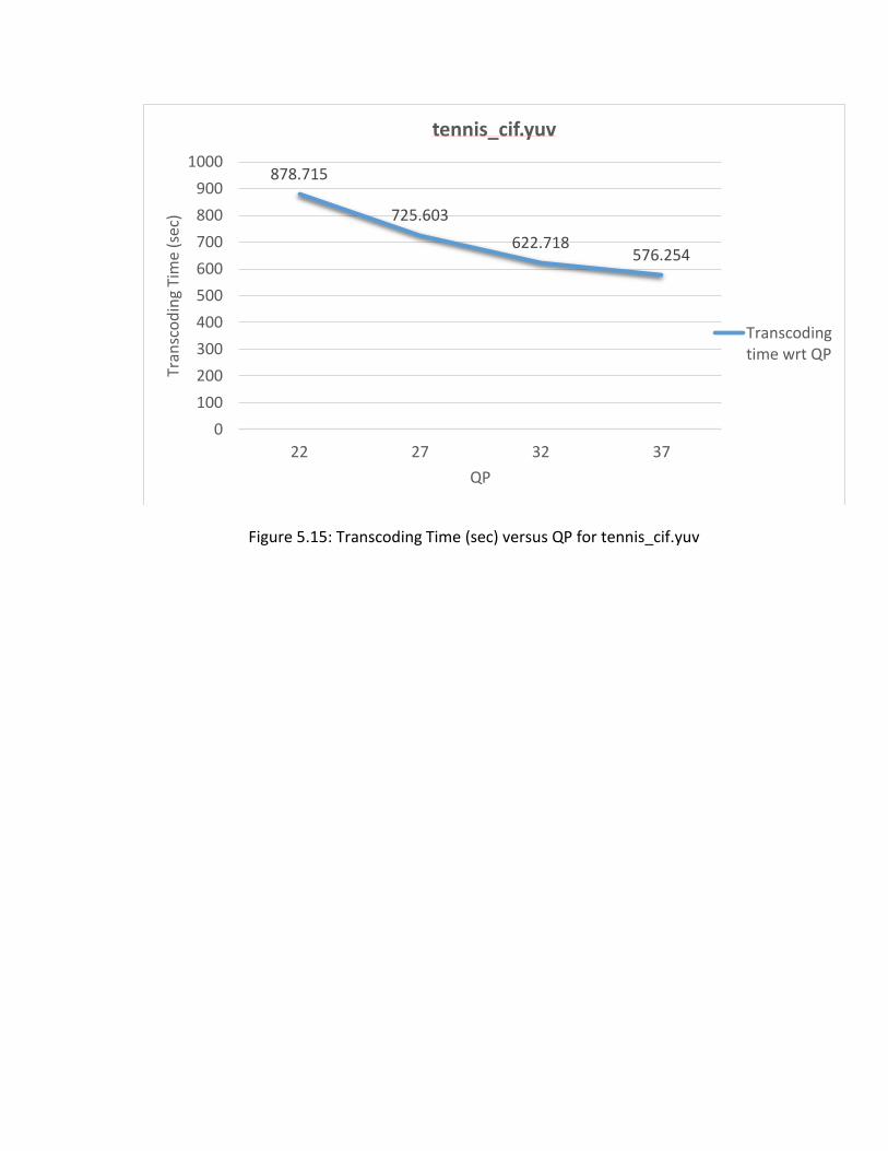
Figure 5.15: Transcoding Time (sec) versus QP for tennis_cif.yuv

878.715

725.603

622.718576.254

0

100

200

300

400

500

600

700

800

900

1000

22 27 32 37

Tran

sco

din

g Ti

me

(sec

)

QP

tennis_cif.yuv


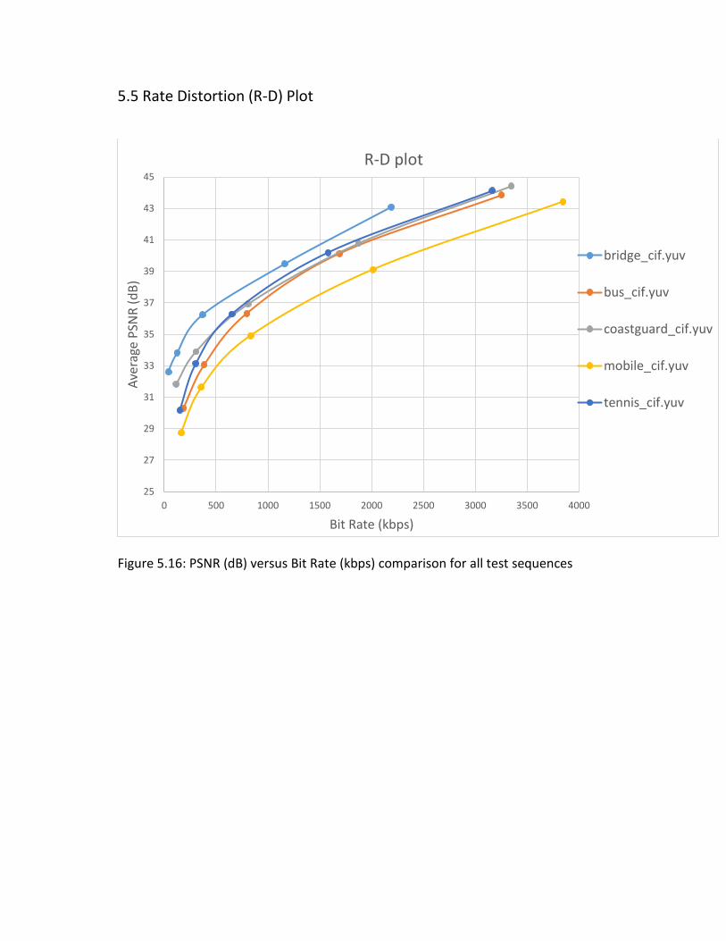
5.5 Rate Distortion (R-D) Plot

Figure 5.16: PSNR (dB) versus Bit Rate (kbps) comparison for all test sequences

25

27

29

31

33

35

37

39

41

43

45

0 500 1000 1500 2000 2500 3000 3500 4000

Ave

rage

PSN

R (

dB

)

Bit Rate (kbps)

R-D plot

bridge_cif.yuv

bus_cif.yuv

coastguard_cif.yuv

mobile_cif.yuv

tennis_cif.yuv

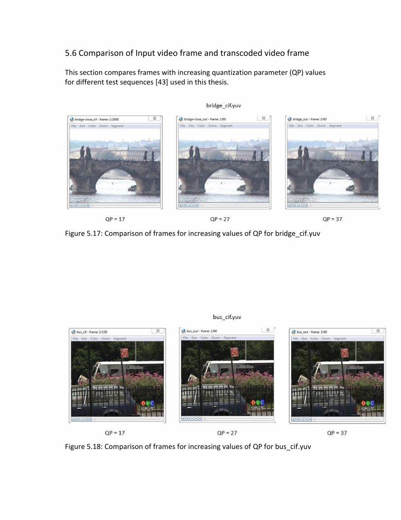
5.6 Comparison of Input video frame and transcoded video frame

This section compares frames with increasing quantization parameter (QP) values for different test sequences [43] used in this thesis.

Figure 5.17: Comparison of frames for increasing values of QP for bridge_cif.yuv

Figure 5.18: Comparison of frames for increasing values of QP for bus_cif.yuv

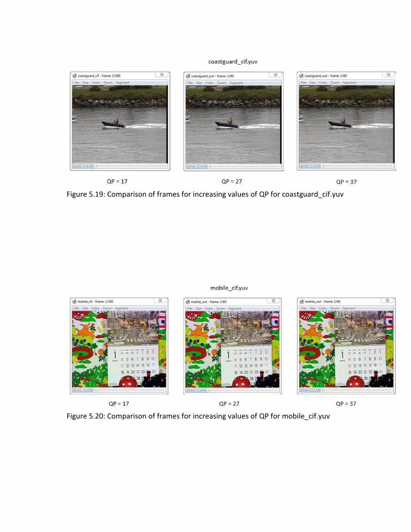
Figure 5.19: Comparison of frames for increasing values of QP for coastguard_cif.yuv

Figure 5.20: Comparison of frames for increasing values of QP for mobile_cif.yuv

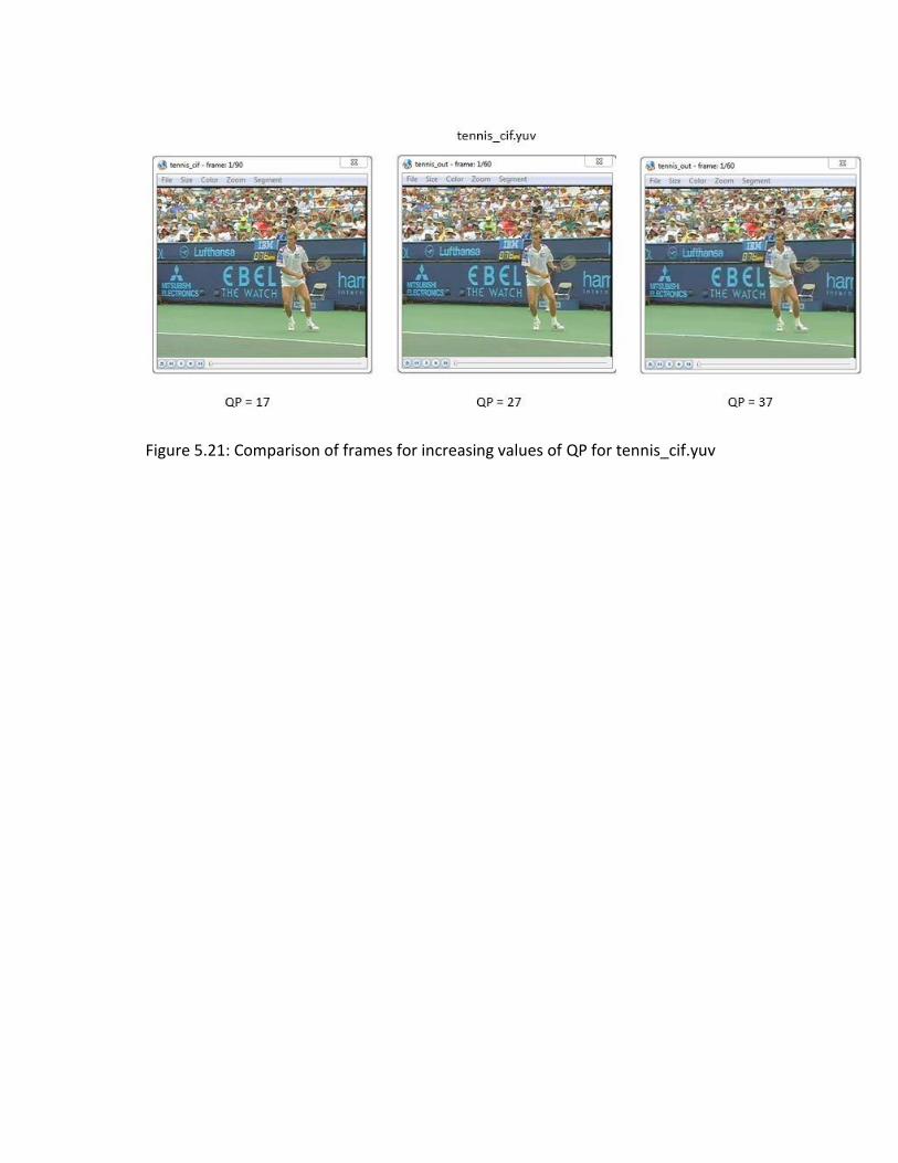
Figure 5.21: Comparison of frames for increasing values of QP for tennis_cif.yuv

6. Conclusions

This thesis focusses on implementing efficient transcoding architecture for

homogeneous transcoding of the new emerging standard: High Efficiency Video

Coding (HEVC) [1, 11]. Transcoding is necessary to enable inter-operability between a

wide range of devices and services used by them. This chapter presents a summary of

the thesis, and explores new research areas that have been identified for further

performance improvement.

6.1 Overview of Transcoder performance

As observed in the results, the cascaded transcoder reduces the transcoding time by

50% when Base QP is increased by 10. The transcoding time is reduced by ~15% to

~26%. Time complexity of this transcoder architecture is high due to full re-encoding

of the bit stream in the transcoder.

It can be observed from the bit rate ratio that the bit rate reduces by ~45% -

~56% for each step increase in the QP value. This bit rate reduction enables HEVC

video stream available for a wide range of devices.

For PSNR values it is observed that there is a reduction in PSNR value with

increase in QP parameter. But, the difference in the PSNR values of the original bit

stream and the transcoded stream is very less and thus indicating that the input and

output video streams are similar. Percentage reduction in average PSNR value is

~8.17% to ~9.72%. For all cases, PSNR values range from 30 dB – 50dB.

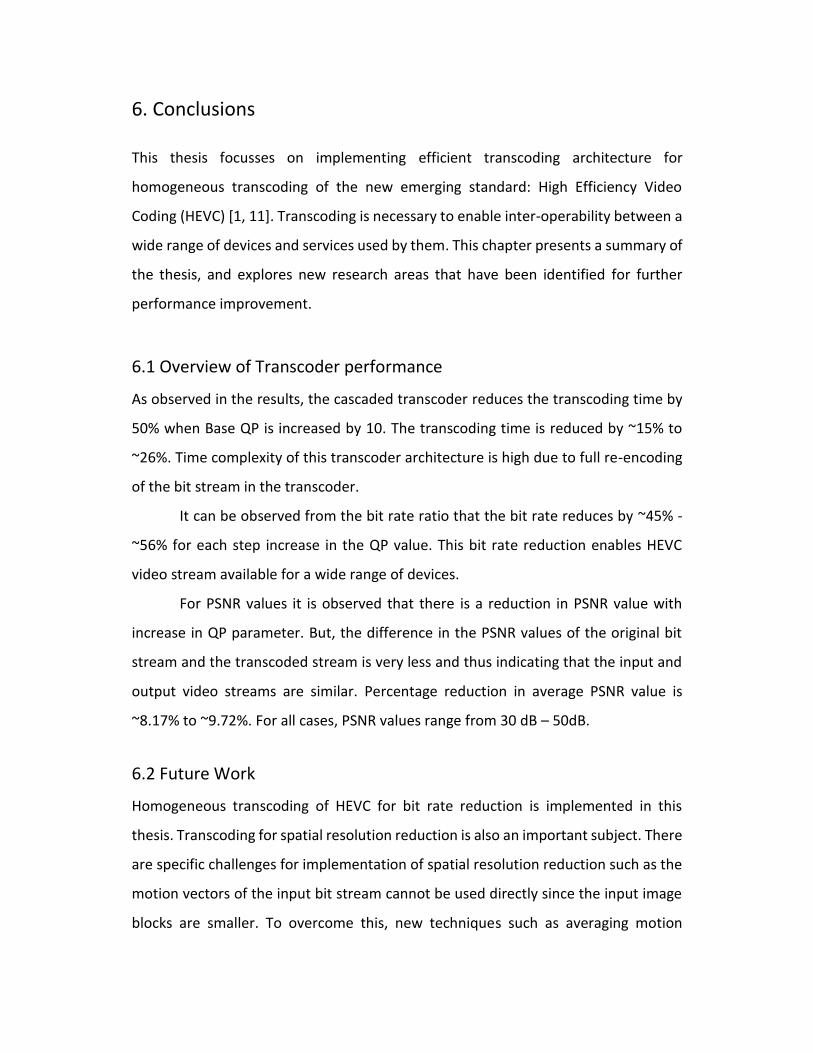
6.2 Future Work

Homogeneous transcoding of HEVC for bit rate reduction is implemented in this

thesis. Transcoding for spatial resolution reduction is also an important subject. There

are specific challenges for implementation of spatial resolution reduction such as the

motion vectors of the input bit stream cannot be used directly since the input image

blocks are smaller. To overcome this, new techniques such as averaging motion

vectors can be developed. Figure 6.1 shows the implementation of spatial resolution

reduction using a downsampler with the proposed transcoder.

The reference implementation of HEVC encoder (HM-11.0) is not meant to

be a real-time encoder. It is interesting to further investigate the performance

implications of using the proposed transcoder models in the real-time encoder

implementations.

Insertion of new information on the video, such as, hidden data, or a layer for

error resilience can also be implemented using this transcoder. Also, this thesis only

studied the effect of transcoding using the low delay main configuration. In HEVC, a

hierarchical configuration (called random access configuration) is also used, due to its

greater rate-distortion efficiency. Implementation of proposed transcoder can be

evaluated with this configuration also.

Figure 6.1: Implementation of spatial resolution reduction using proposed

transcoder.

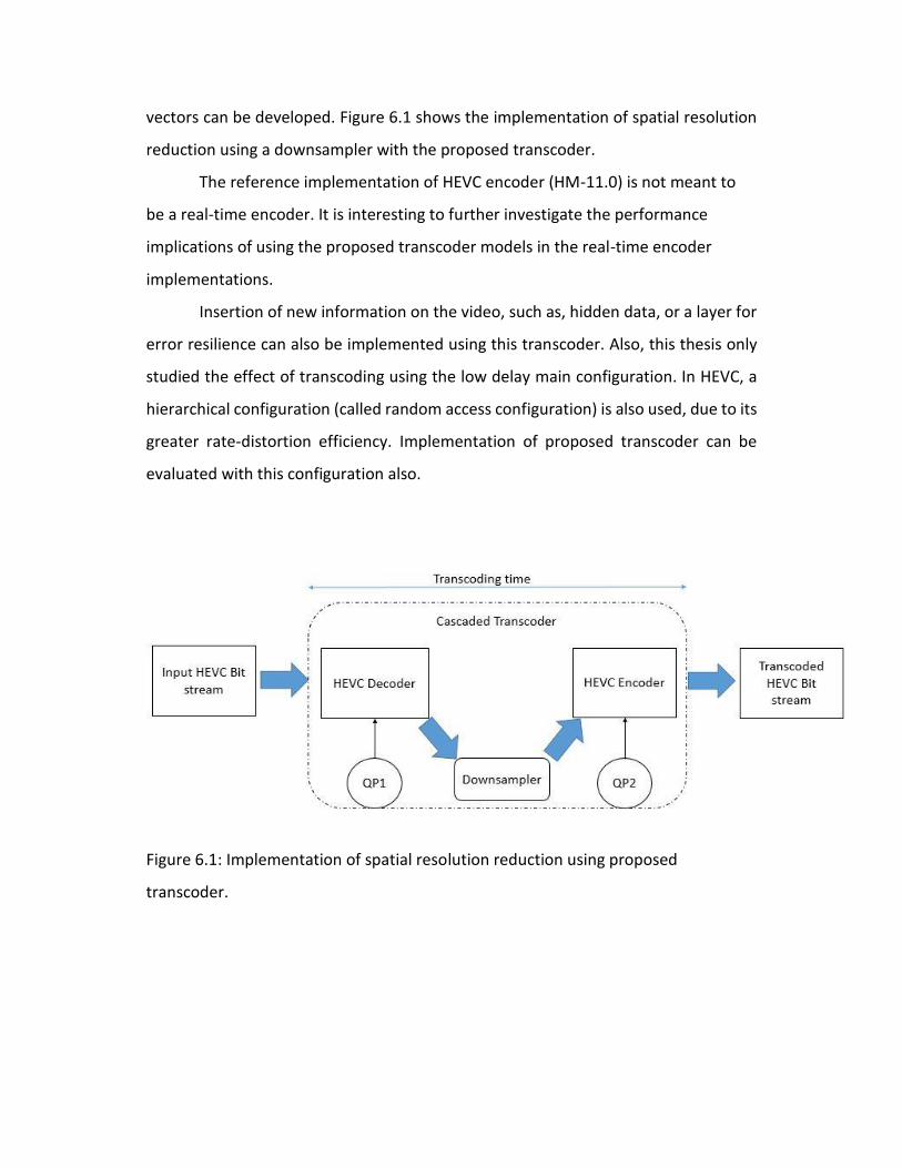
A. Test Sequences

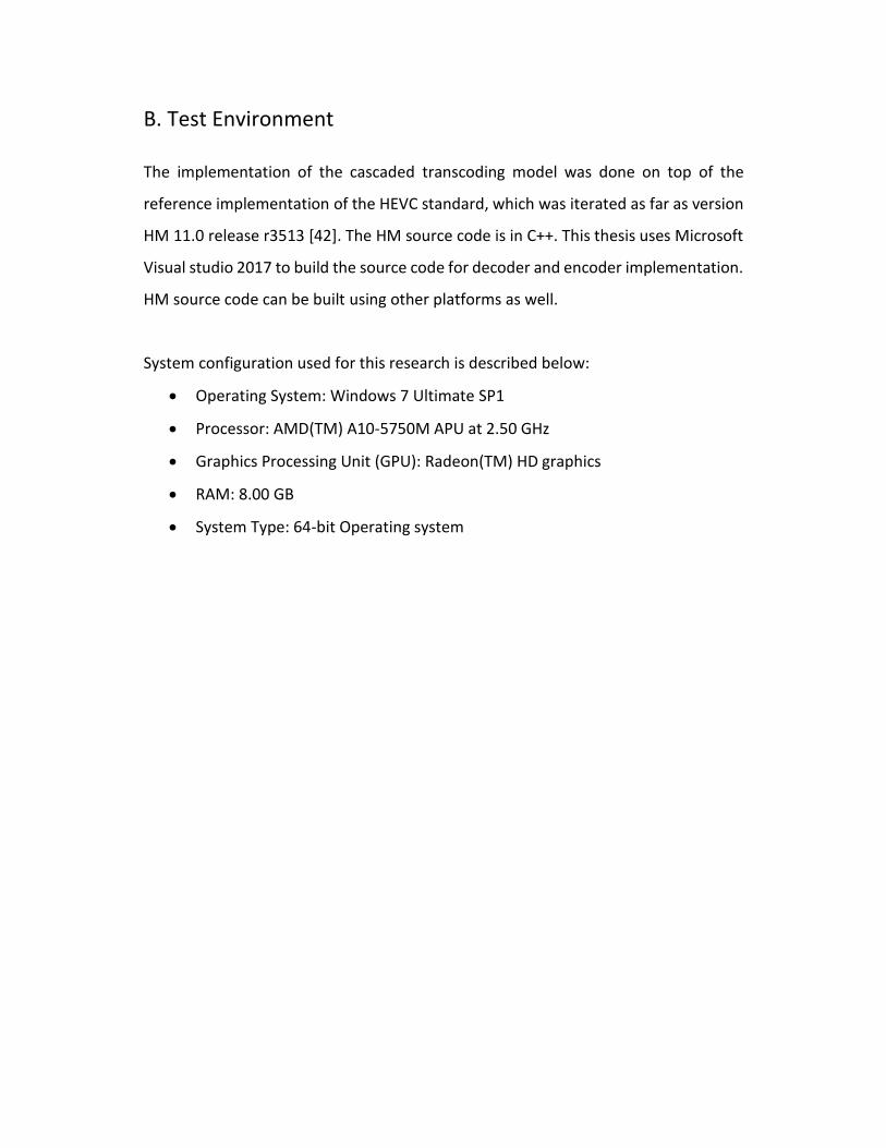
Five test sequences were used for simulation that cover a wide range of real world

scenarios such as complex textures and motion. All the sequences use 4:2:0 YUV color

sampling [43].

Figure A.1: Test sequence bridge_cif.yuv

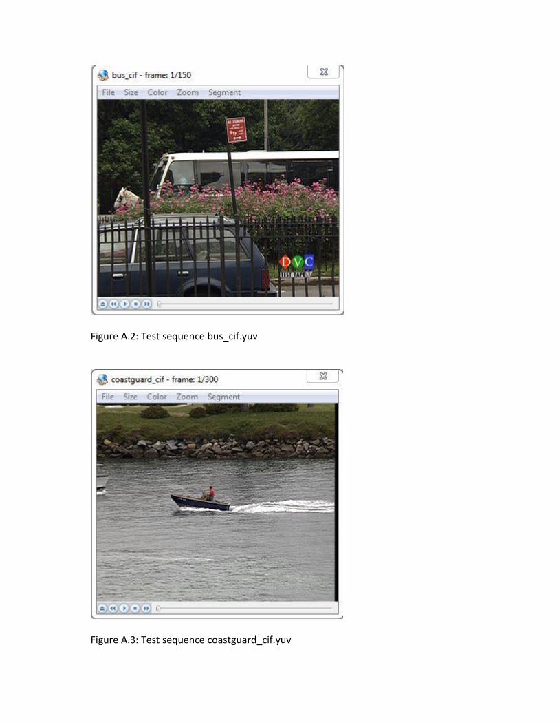
Figure A.2: Test sequence bus_cif.yuv

Figure A.3: Test sequence coastguard_cif.yuv

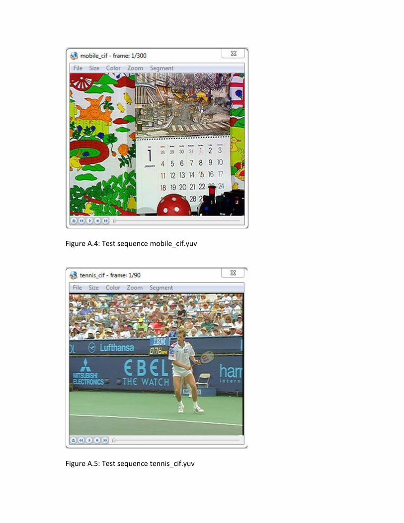
Figure A.4: Test sequence mobile_cif.yuv

Figure A.5: Test sequence tennis_cif.yuv

B. Test Environment

The implementation of the cascaded transcoding model was done on top of the

reference implementation of the HEVC standard, which was iterated as far as version

HM 11.0 release r3513 [42]. The HM source code is in C++. This thesis uses Microsoft

Visual studio 2017 to build the source code for decoder and encoder implementation.

HM source code can be built using other platforms as well.

System configuration used for this research is described below:

Operating System: Windows 7 Ultimate SP1

Processor: AMD(TM) A10-5750M APU at 2.50 GHz

Graphics Processing Unit (GPU): Radeon(TM) HD graphics

RAM: 8.00 GB

System Type: 64-bit Operating system

C. Acronyms

ABR Adaptive Bit rate

AVC Advanced Video Coding

AVS Audio and Video coding Standard

AVS2 Audio and Video coding Standard (Second Generation)

B Frames Bi-directional predicted frames

bpp Bits per pixel

CABAC Context Adaptive Binary Arithmetic Coding

CAVLC Context Adaptive Variable Length Coding

CB Coding Block

CIF Common Intermediate Format

CPU Central Processing Unit

CU Coding Unit

CTB Coding Tree Block

CTU Coding Tree Unit

DCT Discrete Cosine Transform

DF De-blocking Filter

fps Frames per second

GPU Graphics Processing Unit

HD High Definition

HDR High Dynamic Range

HDTV High Definition Television

HE-AAC High Efficiency Advanced Audio Coder

HEVC High Efficiency Video Coding

HHI Heinrich Hertz Institute

I Frames Intra coded frames

ISO International Organization for Standardization

ITS International Telecommunication Symposium

ITU-T Telecommunication Standardization Sector of the

International Telecommunication Union

JCTVC Joint Collaborative Team on Video Coding

JM Joint Model

JPEG Joint Photographic Experts Group

JPEG XR JPEG extended range

JTC Joint Technical Committee

Mbit/s Megabits per second

MC Motion Compensation

ME Motion Estimation

MPEG Moving Picture Experts Group

MSE Mean Square Error

MV Motion Vector

P Frames Predicted frames

PCM Pulse Code Modulation

PSNR Peak-to-peak signal to noise ratio

PU Prediction units

QCIF Quarter Common Intermediate Format

QOE Quality of Experience

QP Quantization Parameter

RAM Random Access Memory

RD Rate distortion

R&D Research and Development

RL Reference Layer

SAO Sample Adaptive Offset

SCC Screen Content Coding

SDCT Steerable Discrete Cosine Transform

SHVC Scalable HEVC

TB Transform Block

TM Trade Mark

TS Test Sequence, Transport Stream

TU Transform Unit

UHD Ultra High Definition

UHDTV Ultra High Definition Television

VC Video Coding

VLC Variable Length Coding

VCEG Visual Coding Experts Group

VQ Vector Quantization

YCbCr Y is the Brightness(luma), Cb is blue minus luma and Cr is red

minus luma

References

1. G. J. Sullivan et al, "Overview of the High Efficiency Video Coding (HEVC)

Standard," in IEEE Trans. on Circuits and Systems for Video Technology, vol. 22, no.

12, pp. 1649-1668, Dec. 2012.

2. J. Xin, C. W. Lin and M. T. Sun, "Digital Video Transcoding," in Proceedings of the

IEEE, vol. 93, no. 1, pp. 84-97, Jan. 2005.

3. ITU-R Recommendation BT.601-6. 601-6 studio encoding parameters of digital

television for standard 4:3 and wide-screen 16:9 aspect ratios. International

Telecommunication Union, 2007.

https://www.itu.int/rec/R-REC-BT.601-7-201103-I/en

4. N. Ahmed, T. Natarajan and K. R. Rao, "Discrete Cosine Transform," in IEEE Trans.

on Computers, vol. C-23, no. 1, pp. 90-93, Jan. 1974.

5. Video Codec for Audiovisual Services at px64 kbit/s, ITU-T Rec. H.261, version 1:

Nov. 1990, version 2: Mar. 1993.

http://www.itu.int/rec/T-REC-H.261/e

6. K. Rijkse, "H.263: video coding for low-bit-rate communication," in IEEE

Communications Magazine, vol. 34, no. 12, pp. 42-45, Dec. 1996.

7. Coding of Moving Pictures and Associated Audio for Digital Storage Media at up to

About 1.5 Mbit/s—Part 2: Video, ISO/IEC 11172-2 (MPEG-1), ISO/IEC JTC 1, 1993.

8. Coding of Audio-Visual Objects—Part 2: Visual, ISO/IEC 14496-2 (MPEG-4 Visual

version 1), ISO/IEC JTC 1, Apr. 1999 (and subsequent editions).

9. Generic Coding of Moving Pictures and Associated Audio Information—Part 2:

Video, ITU-T Rec. H.262 and ISO/IEC 13818-2 (MPEG 2 Video), ITU-T and ISO/IEC JTC

1, Nov. 1994.

10. Advanced Video Coding for Generic Audio-Visual Services, ITU-T Rec. H.264 and

ISO/IEC 14496-10 (AVC), ITU-T and ISO/IEC JTC 1, May 2003 (and subsequent

editions).

11. K. R. Rao, J. J. Hwang and D. N. Kim, “High Efficiency Video Coding and other

emerging standards”, River Publishers 2017.

12. I. Ahmad et al, "Video transcoding: an overview of various techniques and

research issues," in IEEE Trans. on Multimedia, vol. 7, no. 5, pp. 793-804, Oct. 2005.

13. A. Vetro, C. Christopoulos and H. Sun, "Video transcoding architectures and

techniques: an overview," in IEEE Signal Processing Magazine, vol. 20, no. 2, pp. 18-

29, Mar. 2003.

14. J. Xin, M. Sun, K. Chun, “Motion re-estimation for MPEG-2 to MPEG-4 simple

profile transcoding,” in Proceedings of the International Packet Video Workshop,

Pittsburgh, PA, USA, 24–26 Apr. 2002.

15. H. Kalva, “Issues in H.264/MPEG-2 video transcoding,” in Proceedings of the 5th

IEEE Consumer Communications and Networking Conference, pp. 657–659, Las

Vegas, NV, USA, 5–8 Jan. 2004.

16. Z. Zhou et al, “Motion information and coding mode reuse for MPEG-2 to H.264

transcoding,” in Proceedings of the IEEE International Symposium on Circuits and

Systems (ISCAS 2005), Kobe, Japan, pp. 1230–1233, 23–26 May 2005.

17. D. Zhang et al, “Fast Transcoding from H.264 AVC to High Efficiency Video

Coding,” in Proceedings of the IEEE International Conference on Multimedia and

Expo (ICME), Melbourne, Australia, pp. 651–656, 9–13 Jul. 2012.

18. E. Peixoto et al, “H.264/AVC to HEVC Video Transcoder Based on Dynamic

Thresholding and Content Modeling,” in IEEE Trans. Circuits Syst. Video Technology,

pp. 99–112, Jan. 2014.

19. E. Peixoto and E. Izquierdo, “A complexity-scalable transcoder from H.264/AVC

to the new HEVC codec,” in Proceedings of the 19th IEEE International Conference

on Image Processing (ICIP), Orlando, FL, USA, pp. 737–740, 30 Sept. – 3 Oct. 2012.

20. G. Bjontegaard, “Improvements of the BD-PSNR model,” ITU-T SC16/Q6, 35th

VCEG Meeting, Berlin, Germany, Jul. 2008.

21. A.J. Díaz-Honrubia et al, “Adaptive Fast Quadtree Level Decision Algorithm for

H.264 to HEVC Video Transcoding,” in IEEE Trans. on Circuits and Systems for Video

Technology, vol. 26, no. 1, pp. 154-168, Jan. 2016.

22. E.G. Mora et al, “AVC to HEVC transcoder based on quadtree limitation,” in

Multimedia Tools and Applications, pp. 1–25, Springer: Berlin, Germany, 2016.

23. D. Hingole, “H.265 (HEVC) bit stream to H.264 (MPEG 4 AVC) bit stream

transcoder”, M.S. Thesis, EE Dept., University of Texas at Arlington.

http://www.uta.edu/faculty/krrao/dip/


24. B. Wang, Y. Shi, and B. Yin, “Transcoding of H.264 Bitstream to AVS Bitstream,” in

Proceedings of the 5th International Conference on Wireless Communications,

Networking and Mobile Computing, Beijing, China, pp. 1–4, 24–26 Sept. 2009.

25. D. Lefol, D. Bull, and N. Canagarajah, “Performance evaluation of transcoding

algorithms for H. 264,” in IEEE Trans. on Consumer Electronics, vol. 52, no. 1, pp.

215-222, Feb. 2006.

26. B. Bross et al, “High effciency video coding (HEVC) text specification draft 6,” in

ITU-T SG16 WP3 and ISO/IEC JTC1/SC29/WG11, Document JCTVC-H1003, JCT-VC 8th

Meeting, San Jose, CA, USA, pp. 1-10, 2012.

http://phenix.it-sudparis.eu/jct/doc_end_user/current_document.php?id=6465

27. K.L. Cheng, N. Uchihara, and H. Kasai, “Analysis of drift-error propagation in

h.264/avc transcoder for variable bitrate streaming system,” in IEEE Trans. on

Consumer Electronics, vol. 57, no. 2, pp. 888-896, May 2011.

28. S. Kwon, A. Tamhankar, and K. R. Rao, "Overview of the H.264/MPEG-4 part 10,"

in Journal of Visual Communication and Image Representation, vol. 17, is. 9, pp. 186-

216, Apr. 2006.

29. T. Wiegand and G. J. Sullivan, “The H.264 video coding standard”, in IEEE Signal

Processing Magazine, vol. 24, pp. 148-153, Mar. 2007.

30. C. Fogg, “Suggested figures for the HEVC specification”, ITU-T/ISO/IEC Joint

Collaborative Team on Video Coding (JCT-VC) document JCTVC-J0292rl, Jul. 2012.

31. AVC Reference software manual:

http://vc.cs.nthu.edu.tw/home/courses/CS553300/97/project/JM%20Reference%20

Software%20Manual%20(JVT-X072).pdf

32. MPL Website: http://www.uta.edu/faculty/krrao/dip/

33. High Efficiency Video Coding (HEVC) text specification draft 8:


34. P. Kunzelmann and H. Kalva, “Reduced complexity H.264 to MPEG-2 transcoder”,

In IEEE International Conference on Consumer Electronics (ICCE 2007), pp. 1–2, Jan.

2007.

35. T. Shanableh and M. Ghanbari, “Heterogeneous video transcoding to lower

spatio-temporal resolutions and different encoding formats”, in IEEE Trans. on

Multimedia, pp. 101–110, Jun. 2000.

36. H. Sun, W. Kwok, and J.W. Zdepski, “Architectures for MPEG compressed bit-

stream scaling”, in IEEE Trans. on Circuits and Systems for Video Technology,

pp. 191–199, Apr. 1996.

37. P.A.A. Assuncao and M. Ghanbari, “Transcoding of MPEG-2 video in the

frequency domain”, In IEEE International Conference on Acoustics, Speech, and

Signal Processing (ICASSP 1997), volume 4, pp. 2633 –2636, Apr. 1997.

38. P. Yin et al, “Drift compensation for reduced spatial resolution transcoding”, in

IEEE Trans. on Circuits and Systems for Video Technology, volume 12, pp. 1009–1020,

Nov. 2002.



39. Z. Chen and K.N. Ngan, “Recent advances in rate control for video coding”, in

Signal Processing: Image Communication, volume 22, pp. 19-38, Jan. 2007.

40. N. Bjork and C. Christopoulos, “Transcoder architectures for video coding”, in

IEEE Trans. on Consumer Electronics, volume 44, pp. 88–98, Feb. 1998.

41. P. Yin, A. Vetro, B. Liu, and H. Sun, “Drift compensation for reduced spatial

resolution transcoding”, In IEEE Trans. on Circuits and Systems for Video

Technology, volume 12, pp. 1009–1020, Nov. 2002.

42. HEVC reference software link:

https://hevc.hhi.fraunhofer.de/svn/svn_HEVCSoftware/trunk/build/

43. Test sequences link:

http://trace.eas.asu.edu/yuv/index.html

https://media.xiph.org/video/derf/

44. AVC/H.264 reference software link:

http://iphome.hhi.de/suehring/tml/download/

45. V. Sze, M. Budagavi, and G. J. Sullivan. "High efficiency video coding

(HEVC)." Integrated Circuit and Systems, Algorithms and Architectures.

Springer (2014): pp. 1-375.

46. S. Ma, S. Wang, W. Gao, “Overview of IEEE 1857 video coding standard”, In

Proceedings of the IEEE International Conference on Image Processing, Melbourne,

Australia, pp. 1500–1504, 15–18 Sept. 2013.

https://hevc.hhi.fraunhofer.de/svn/svn_HEVCSoftware/trunk/build/

http://trace.eas.asu.edu/yuv/index.html

https://media.xiph.org/video/derf/

http://iphome.hhi.de/suehring/tml/download/

47. University of Texas at Austin (ECE Department):

https://users.ece.utexas.edu/~ryerraballi/MSB/ppts/

48. G. Tech et al, “Overview of the multiview and 3D extensions of high efficiency

video coding”, IEEE Trans. on Circuits and Systems for Video Technology, pp.35-49,

Jan. 2016.

49. J. Zhang et al, “Efficient HEVC to H.264/AVC transcoding with fast intra mode

decision”, In International Conference on Multimedia Modeling, Springer Berlin

Heidelberg, pp. 295-306, Jan. 2013.

Useful Tutorials on Video Processing:

1. http://kohtoomaung.blogspot.com/p/blog-page_10.html

2. https://codesequoia.wordpress.com/2012/11/04/

https://users.ece.utexas.edu/~ryerraballi/MSB/ppts/

http://kohtoomaung.blogspot.com/p/blog-page_10.html

https://codesequoia.wordpress.com/2012/11/04/

HOMOGENEOUS TRANSCODING OF HEVC (H.265) - … TRANSCODING OF HEVC (H.265) ... MPEG-4 visual and...

Documents

Transcript of HOMOGENEOUS TRANSCODING OF HEVC (H.265) - … TRANSCODING OF HEVC (H.265) ... MPEG-4 visual and...