
Holtmann75 / Module Math 75 Holtmann Revised 2015-11-18.pdf
287
p. i Math 75 Linear Algebra Class Notes Prof. Erich Holtmann For use with Elementary Linear Algebra, 7 th ed., Larson Revised 21-Nov-2015
Transcript of Holtmann75 / Module Math 75 Holtmann Revised 2015-11-18.pdf

p. i
Math 75
Linear Algebra
Class Notes
Prof. Erich Holtmann
For use with
Elementary Linear Algebra,
7th
ed., Larson
Revised 21-Nov-2015


p. i
Contents
Chapter 1: Systems of Linear Equations 1
1.1 Introduction to Systems of Equations. 1
1.2 Gaussian Elimination and Gauss-Jordan Elimination. 9
1.3 Applications of Systems of Linear Equations. 15
Chapter 2: Matrices. 19
2.1 Operations with Matrices. 19
2.2 Properties of Matrix Operations. 23
2.3 The Inverse of a Matrix. 27
2.4 Elementary Matrices. 31
2.5 Applications of Matrix Operations. 37
Chapter 3: Determinants. 41
3.1 The Determinant of a Matrix. 41
3.2 Determinants and Elementary Operations. 45
3.3 Properties of Determinants. 51
3.4 Applications of Determinants. 55
Chapter 4: Vector Spaces. 61
8.1 Complex Numbers (Optional). 61
8.2 Conjugates and Division of Complex Numbers (Optional). 67
4.1 Vectors in Rn. 71
4.2 Vector Spaces. 77
4.3 Subspaces of Vector Spaces. 82
4.4 Spanning Sets and Linear Independence. 86
4.5 Basis and Dimension. 97
4.6 Rank of a Matrix and Systems of Linear Equations. 105
4.7 Coordinates and Change of Basis. 117
Chapter 5: Inner Product Spaces. 121
5.1 Length and Dot Product in Rn. 121
5.2 Inner Product Spaces. 129
5.3 Orthogonal Bases: Gram-Schmidt Process. 137
5.4 Mathematical Models and Least Squares Analysis (Optional). 145
5.5 Applications of Inner Product Spaces (Optional). 151
8.3 Polar Form and De Moivre's Theorem. (Optional) 157
8.4 Complex Vector Spaces and Inner Products. 163

p. ii
Chapter 6: Linear Transformations. 169
6.1 Introduction to Linear Transformations. 169
6.2 The Kernel and Range of a Linear Transformation. 175
6.3 Matrices for Linear Transformations. 183
6.4 Transition Matrices and Similarity. 191
6.5 Applications of Linear Transformations. 193
Chapter 7: Eigenvalues and Eigenvectors. 201
7.1 Eigenvalues and Eigenvectors. 201
7.2 Diagonalization. 209
7.3 Symmetric Matrices and Orthogonal Diagonalization. 215
7.4 Applications of Eigenvalues and Eigenvectors. 223
8.5 Unitary and Hermitian Spaces. 223

Chapter 1: Systems of Linear Equations
1.1 Introduction to Systems of Equations.
p. 1
Chapter 1: Systems of Linear Equations
1.1 Introduction to Systems of Equations.
Objective: Recognize and solve mn systems of linear equations by hand using Gaussian
elimination and back-substitution.
a1x1 + a2x2 + … + anxn = b is a linear equation in standard form in n variables xi.
The first nonzero coefficient ai is the leading coefficient. The constant term is b.
Compare to the familiar forms of linear equation s in two variables y = mx + b and x = a.
Example: Linear and Nonlinear Equations
(sin ) x1 – 4x2 = e2
sin x1 + 2x2 – 3x3 = 0
Linear Nonlinear
An mn system of linear equations is a set of m linear equations in n unknowns.
Example: Systems of Two Equations in Two Variables
Solve and graph each 22 system.
a. 2x – y = 1
x + y = 5
b. 2x – y = 1
–4x + 2y = –2
c. 2x – y = 1
–4x + 2y = 5
For a system of linear equations, exactly one of the following is true.
1) The system has exactly one solution (consistent, nonsingular system).
2) The system has infinitely many solutions (consistent, singular system).
Use a free parameter or free variable (or several free parameters) to represent the solution set.
3) The system has no solution (inconsistent, singular system).

Chapter 1: Systems of Linear Equations
1.1 Introduction to Systems of Equations.
p. 2
To solve mn systems of linear equations (when m and n are large) we use a procedure called
Gaussian elimination to find an equivalent system of equations in row-echelon form. Then we
use back-substitution to solve for each variable.
Row-echelon form means that the leading coefficients of 1 (called “pivots”) and the zero terms
below them form a stair-step pattern. You could walk downstairs from the top left. You might
have to move more than one column to the right to reach the next step, but you never have to
step down more than one row at a time.
Row-echelon form
91
841
11
731251
5
54
3
54321
x
xx
x
xxxxx
Row-echelon form
00
00
11
731251
3
54321
x
xxxxx
Not row-echelon form
931
8421
1231
731251
54
543
543
54321
xx
xxx
xxx
xxxxx
The goal of Gaussian elimination is to find an equivalent system that is in row-echelon form. The
three operations you can use during Gaussian elimination are
1) Swap the order of two equations.
2) Multiply an equation on both sides by a non-zero constant.
3) Add a multiple of one equation to another equation.
In Gaussian elimination, you start with Equation 1 (the first equation of your mn system).
1) Find the leading coefficient in the current equation. (Sometimes you need to swap
equations in this step.)
2) Eliminate the coefficients of the corresponding variable in all of the equations below the
current equation.
3) Move down to the next equation and go back to Step 1. Repeat until you run out of
equations or you run out of variables.
Solve using back-substitution: solve the last equation for the leading variable, then substitute into
the preceding (i.e. second-to-last) equation and solve for its leading variable, then substitute into
the preceding equation and solve for its leading variable, etc. Variables that are not leading
variables are free parameters, and we often set them equal to t, s, ….

Chapter 1: Systems of Linear Equations
1.1 Introduction to Systems of Equations.
p. 3
Examples: Gaussian Elimination and Back-Substitution on 33 Systems of Linear Equations.

Chapter 1: Systems of Linear Equations
1.1 Introduction to Systems of Equations.
p. 4
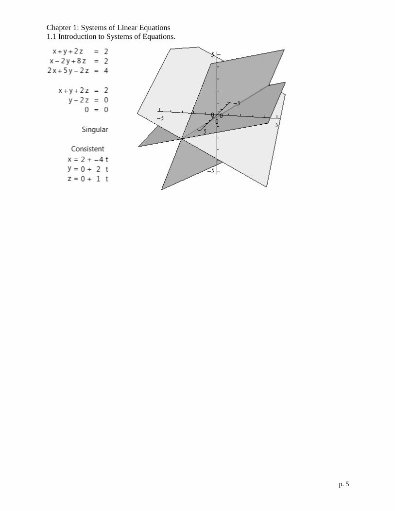
Chapter 1: Systems of Linear Equations
1.1 Introduction to Systems of Equations.
p. 5
Chapter 1: Systems of Linear Equations
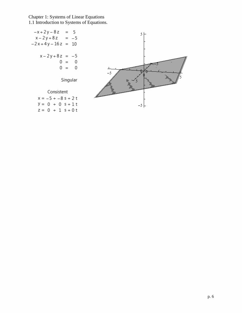
1.1 Introduction to Systems of Equations.
p. 6

Chapter 1: Systems of Linear Equations
1.1 Introduction to Systems of Equations.
p. 7
Example: Chemistry Application
Write and solve a system of linear equations for the chemical reaction
(x1)CH4 + (x2)O2 (x3)CO2 + (x4)H2O
Solution: write a separate equation for each element, showing the balance of that element.
C: 1x1 + 0x2 = 1x3 + 0x4 so 1x1 + 0x2 – 1x3 + 0x4 = 0
H: 4x1 + 0x2 = 0x3 + 2x4 so 4x1 + 0x2 + 0x3 – 2x4 = 0
O: 0x1 + 2x2 = 2x3 + 1x4 so 0x1 + 2x2 – 2x3 – 1x4 = 0


Chapter 1: Systems of Linear Equations
1.2 Gaussian Elimination and Gauss-Jordan Elimination.
p. 9
1.2 Gaussian Elimination and Gauss-Jordan Elimination.
Objective: Use matrices and Gauss-Jordan elimination to solve mn systems of linear equations
by hand and with software.
Objective: Use matrices and Gaussian elimination with back-substitution to solve mn systems
of linear equations by hand and with software.
Use row-echelon form or reduced row-echelon form to determine the number of solutions of a
homogeneous system of linear equations, and (if applicable) the number of free parameters.
A matrix is a rectangular array of numbers, called matrix
entries, arranged in horizontal rows and vertical columns.
Matrices are denoted by capital letters; matrix entries are
denoted by lowercase letters with two indices. In a given
matrix entry aij, the first index i is the row, and the second
index j is the column. The entries a11, a22, a33, … compose the
main diagonal. If m = n then A is called a square matrix.
A linear system
mnmnmmm
nn
nn
bxaxaxaxa
bxaxaxaxa
bxaxaxaxa
332211
22323222121
11313212111
can represented either by a coefficient matrix A and a column vector b
mnmmm
n
n
n
aaaa
aaaa
aaaa
aaaa
A
331
3333231
2232221
1131211
and
mb
b
b
b
3
2
1
b
or by an augmented matrix M, which I will sometimes write as [A | b]
mmnmmm
n
n
n
baaaa
baaaa
baaaa
baaaa
M
331
33333231
22232221
11131211
(The book, Mathematica, and the calculator do not display the dotted vertical line.)
To create M in Mathematica from A and b, type m=Join[a,b,2]
To create M on the TI-89 from A and b, type
Matrixaugment(A
B
M
mnmmm
n
n
n
aaaa
aaaa
aaaa
aaaa
A
321
3333231
2232221
1131211

Chapter 1: Systems of Linear Equations
1.2 Gaussian Elimination and Gauss-Jordan Elimination.
p. 10
In a similar manner to that used for an mn system of linear equations, we can use a Gaussian
elimination on the coefficient side A of the augmented matrix [A | b] to find an equivalent
augmented matrix [U | c] in row-echelon form. Then we use back-substitution to solve for each
variable. U is called an upper triangular matrix because all non-zero entries are on or above the
main diagonal.
row-echelon form row-echelon form not row-echelon form
20000
41000
50100
31251
00000
00000
50100
31251
31000
42100
23100
31251
Example: Use Gaussian elimination and back-substitution to solve. The three elementary row
operations you can use during Gaussian elimination are
1) Swap the two rows.
2) Multiply a row by a non-zero constant.
3) Add a multiple of one row to another row.
2111
3123
8346
zyx
zyx
zyx
2111
3123
8346
2100
210
1
23
34
21
32
1)2()1( so
1)2(2 so 2
2
21
32
34
34
21
32
23
23
xzyx
yzy
z
Steps:

Chapter 1: Systems of Linear Equations
1.2 Gaussian Elimination and Gauss-Jordan Elimination.
p. 11
Instead of using back-substitution, we can take the row-echelon form [U | c] and eliminate the
coefficients above the pivots by adding multiples of the pivot rows. The result [R | d] is called
reduced row-echelon form.
reduced row-echelon form reduced row-echelon form
20000
41000
50100
110051
30000
40000
23100
31051
Example: Use Gauss-Jordan elimination to solve.
2111
3123
8346
zyx
zyx
zyx
2111
3123
8346
2100
210
1
23
34
21
32
2100
1010
1001
2
1
1
z
y
x

Chapter 1: Systems of Linear Equations
1.2 Gaussian Elimination and Gauss-Jordan Elimination.
p. 12
Example Using software to find the Reduced Row-Echelon Form (Exercise 1.2 #39)
Mathematica
Go to the Palettes Menu and open the Basic Math
Assistant. Under Basic Commands, open the Matrix
Tab.
Type a=
and click
Use the Add Row and Add Column buttons to expand
the matrix, so you can enter the augmented matrix
(If you make the matrix to large, use to remove rows and columns.) Press (or
on the number pad) when you are finished entering the augmented matrix.
Another way to enter the augmented matrix is to type (or download) a={{1,-1,2,2,6,6},{3,-2,4,4,12,14},{0,1,-1,-1,-3,-3},{2,-
2,4,5,15,10},{2,-2,4,4,13,13}}
MatrixForm[a]
You can download this matrix from http://holtmann75.pbworks.com. Click on Electronic
Data Sets and open 1133110878_323834.zip/DataSets/Mathematica/0102039.nb (Ch. 01,
Section 02, Problem 039). Notice that A and a are different variables! User-defined variables
should always begin with a lower-case letter, because Mathematica’s built-in fuctions and
commands begin with capital letters. (For example, N and C are already defined by
Mathematica.)
On the Basic Math Assistant palette, click on MatrixForm RowReduce and type a so you have
MatrixForm[RowReduce[a]]
Converting back to a system of linear equations, we have
x1 = 2 x4 = 5
x2 = 2 x5 = 1
x3 = 3

Chapter 1: Systems of Linear Equations
1.2 Gaussian Elimination and Gauss-Jordan Elimination.
p. 13
TI-89: Type
Data/Matrix Editor
New...
Type: Matrix
Folder: main
Variable: A
(A is above . If you type = instead of a, use .
If a already exists, then use Open... on the previous
screen instead of New....)
Use and the
arrow keys to type
in the coefficient matrix
(If you need to insert or delete a row or column, use )
When you are finished, press .
Another way to enter the matrix is to type (from the
home screen) 1,1,2,2,6,6
3,2,4,4,12,14
0,1,1,1,3,3
2,2,4,5,15,10
2,2,4,4,13,13
A
After the matrix is entered, type A
Matrix rref( A
Converting back to a system of linear equations, we have
x1 = 2
x2 = 2
x3 = 3
x4 = 5
x5 = 1

Chapter 1: Systems of Linear Equations
1.2 Gaussian Elimination and Gauss-Jordan Elimination.
p. 14
Mathematica can help you perform row operations. If your augmented matrix is in a, then
a[[2]] is row 2 of the matrix. To view a in the usual format, type
MatrixForm[a]
To swap rows 2 and 3 of a, type a[[{2,3}]]=a[[{3,2}]]
To multiply row 2 of a by 7, type a[[2]]=7*a[[2]]
To add 7 times row 2 to row 1, type a[[1]]=a[[1]]+7*a[[2]]
Mathematica performs operations in the order that you type them in, not as they appear on the
screen. If you go back and edit your work, you can use Evaluate Notebook under the Evaluation
menu to recalculate the notebook in the order on the screen.
The TI-89 can also help you perform row operations. If your augmented matrix is in a, then …
To swap rows 2 and 3 of a and store the result in a1, type
Matrix Row opsrowSwap(A,2,3,)
A1
To multiply row 2 of a1 by 7 and store the result in a2, type
Matrix Row opsmRow(7,A1,2)
A2
To add 7 times row 2 of a2 to row 1 and store the result in a3, type
Matrix Row opsmRowAdd(7,A2,1,3)
A3
About notation:
43
21 and
43
21 are matrices, but
43
21 is a determinant (Ch. 3).
Theorem 1.1. Every homogeneous (constants on right-hand side are all zeroes) system of linear
equations is consistent. The number of free parameters in the solution set is the number of
variables minus the number of pivots (leading coefficients). If there are zero free parameters,
then there is exactly one solution.
Examples:
0112
0201
0511
0121428205
0559211
011150
042511
02131500
0377208
0454156
012352
Solutions:
0000
0310
0201
Chapter 1: Systems of Linear Equations
1.3 Applications of Systems of Linear Equations.
p. 15
1.3 Applications of Systems of Linear Equations.
Objective: Set up and solve a system of equations to fit a polynomial function to a set of data
points.
Objective: Set up and solve a system of equations to represent a network.
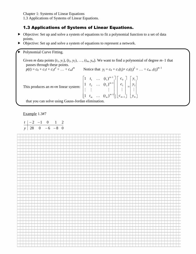
Polynomial Curve Fitting.
Given m data points (t1, y1), (t2, y2), …, (tm, ym). We want to find a polynomial of degree m–1 that
passes through these points.
p(t) = c0 + c1t + c2t2 + … + cmt
m Notice that yj = c0 + c1(tj)+ c2(tj)
2 + … + cm–1(tj)
m–1
This produces an mm linear system:
1
1
22
1
11
)(1
)(1
)(1
m
mm
m
m
tt
tt
tt
1
1
0
mc
c
c
=
my
y
y
2
1
that you can solve using Gauss-Jordan elimination.
Example 1.3#7
086028
21012
y
t

Chapter 1: Systems of Linear Equations
1.3 Applications of Systems of Linear Equations.
p. 16
Example 1.3#9
1275
200820072006
y
t
Network Analysis: write a system of linear equations using Kirchoff’s Laws.
1) Flow into each node (also called vertex) equals flow out.
2) In an electrical network, the sum of the products IR (I = current and R = resistance) around
any closed path of edges (lines) is equal to the total voltage in the loop from the batteries.
A resistor is represented by the symbol Resistance is measured in ohms ().
1 k = 1000
A battery is represented by the symbol If the current flows through the battery
from the short line (–) to the long line
(+), then the voltage is positive.
Current is measure in amps (A). 1 mA = 0.001 A.
Flow into a node is positive. Flow out of a node is negative.
To write a system of equations,
1) Pick a direction (at random) for each current I.
2) For each node, write an equation for the current input and output.
3) For each loop, write the V = IR equation.
I
Chapter 1: Systems of Linear Equations
1.3 Applications of Systems of Linear Equations.
p. 17
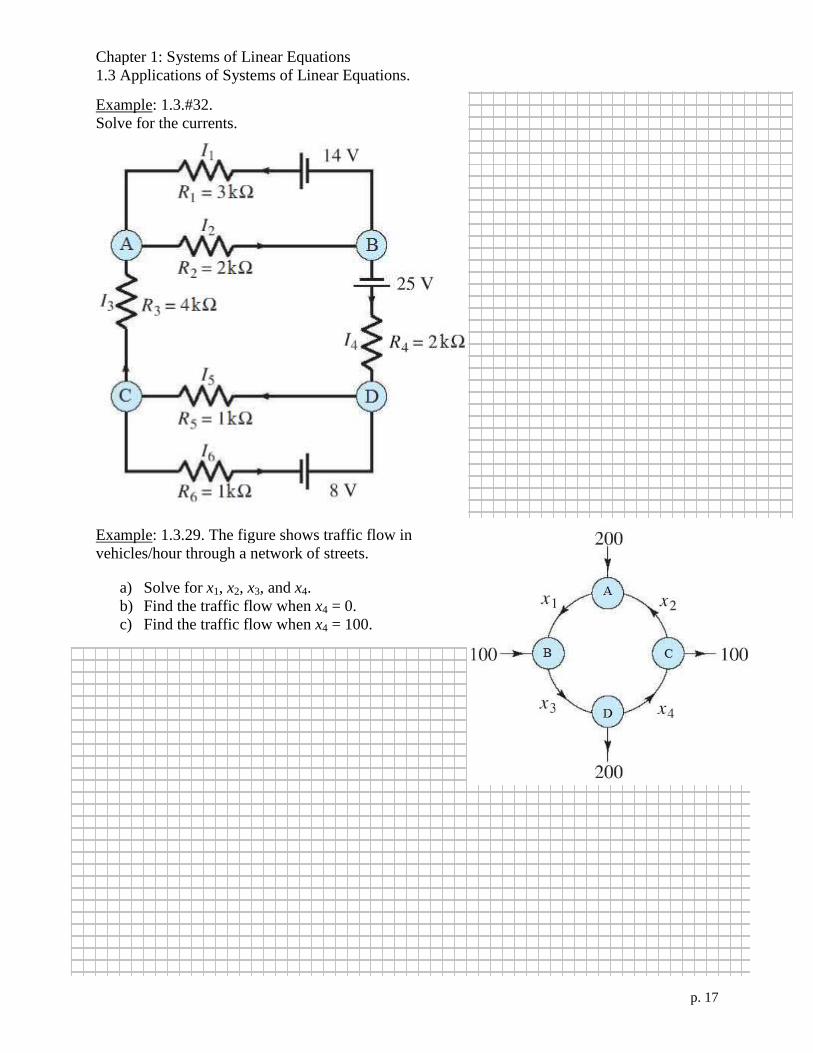
Example: 1.3.#32.
Solve for the currents.
Example: 1.3.29. The figure shows traffic flow in
vehicles/hour through a network of streets.
a) Solve for x1, x2, x3, and x4.
b) Find the traffic flow when x4 = 0.
c) Find the traffic flow when x4 = 100.

Chapter 2: Matrices.
2.1 Operations with Matrices.
p. 19
Chapter 2: Matrices.
2.1 Operations with Matrices.
Objective: Determine whether or not two matrices are equal.
Objective: Add and subtract matrices and multiply a matrix by a scalar.
Objective: Multiply two matrices.
Objective: Write solutions to a system of linear equations in column vector notation.
Objective: Partition a matrix and perform block multiplication.
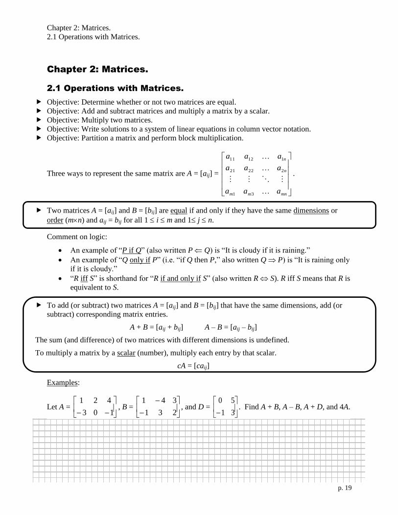
Three ways to represent the same matrix are A = [aij] =
mnmm
n
n
aaa
aaa
aaa
31
22221
11211
.
Two matrices A = [aij] and B = [bij] are equal if and only if they have the same dimensions or
order (mn) and aij = bij for all 1 i m and 1 j n.
Comment on logic:
An example of “P if Q” (also written P Q) is “It is cloudy if it is raining.”
An example of “Q only if P” (i.e. “if Q then P,” also written Q P) is “It is raining only
if it is cloudy.”
“R iff S” is shorthand for “R if and only if S” (also written R S). R iff S means that R is
equivalent to S.
To add (or subtract) two matrices A = [aij] and B = [bij] that have the same dimensions, add (or
subtract) corresponding matrix entries.
A + B = [aij + bij] A – B = [aij – bij]
The sum (and difference) of two matrices with different dimensions is undefined.
To multiply a matrix by a scalar (number), multiply each entry by that scalar.
cA = [caij]
Examples:
Let A =
103
421, B =
231
341, and D =
31
50. Find A + B, A – B, A + D, and 4A.

Chapter 2: Matrices.
2.1 Operations with Matrices.
p. 20
In Mathematica, use a+b, a–b, and 4*a or 4a to add matrices, subtract matrices, and multiply
scalars c by matrices. Remember, you can enter D =
31
50 from the Palettes Menu::Basic
Math Assistant::Basic Commands::Matrix Tab.
On the TI-89, use ab, a b, and ca or 4a to add matrices A and B, subtract matrices,
and multiply scalars c by matrices. Remember, you can enter D =
31
50 from the home screen
as [0,5;-1,3]D or from Data/Matrix Editor. (Be sure to use
Type: Matrix)
Matrix multiplication is defined in a much more complex manner. For a 11 system, we can
write ax = b. We want a definition of matrix multiplication that allows us to write an mn system
mnmnmmm
nn
nn
bxaxaxaxa
bxaxaxaxa
bxaxaxaxa
332211
22323222121
11313212111
as Ax = b,
where A is the coefficient matrix
mnmm
n
n
aaa
aaa
aaa
A
21
22221
11211
,
and x and b are column matrices (or column vectors):
nx
x
x
2
1
x and
mb
b
b
2
1
b .
Observe that each row of A was multiplied by the column x to give the corresponding row of b.
If A = [aij] is an mn matrix and B = [bij] is an np matrix, then the product AB is an mp matrix
A = [cij] where
[cij] =
n
k
kjikba1
= ai1b1j + ai2b2j + ai3b3j + … ainbnj
If the column dimension of A does not match the row dimension of B, then the product is
undefined

Chapter 2: Matrices.
2.1 Operations with Matrices.
p. 21
Examples
52
33
23
32
512
014
In Mathematica, use a.b to multiply matrices.(Do not use a*b)
On the TI-89, use ab multiply matrices.
Example: Write solutions to a system of linear equations in column vector notation.
Solve
2110
1011
3121
4
3
2
1
x
x
x
x
=
0
0
0
4
3
2
1
x
x
x
x
= t
1
1
1
2
Block multiplication on partitioned matrices works whenever the dimensions are OK.
Examples
2221
1211
1200
0001
0010
AA
AAA with
1200
00
00
01
10
2221
1211
AA
AA and
2221
1211
265
134
011
021
BB
BBB with
2
1
65
34
0
0
11
21
2221
1211
BB
BB
Then AB =
2222122121221121
2212121121121111
BABABABA
BABABABA =
2222212211
2211211111
000
000
BABAB
BABBA=
01213
021
011

Chapter 2: Matrices.
2.1 Operations with Matrices.
p. 22
Ax=
mnmm
n
n
aaa
aaa
aaa
21
22221
11211
nx
x
x
2
1
=
nmnmm
nn
nn
xaxaxa
xaxaxa
xaxaxa
2211
2222121
1212111
=n
mn
n
n
mm
x
a
a
a
x
a
a
a
x
a
a
a
2
1
2
2
22
12
1
1
21
11
In block matrix notation, we write [ a1 | a2 | … | an ] =
mnmm
n
n
aaa
aaa
aaa
21
22221
11211
where the ai are
m1 column matrices. The Ax = [ a1 | a2 | … | an ]
nx
x
x
2
1
= a1x1 + a2x2 + … + anxn
Similarly, if B is an lm matrix (so BA is defined), then
BA = B[ a1 | a2 | … | an ] = [ Ba1 | Ba2 | … | Ban ], i.e. the columns of BA are Bai.
Notice that B is lm, ai is m1, Bai is l1, and BA is ln.
On the other hand, we could partition A into 1m row matrices ri
A =
mnmm
n
n
aaa
aaa
aaa
21
22221
11211
=
mr
r
r
2
1
. Then Ax =
mnmm
n
n
aaa
aaa
aaa
21
22221
11211
nx
x
x
2
1
=
mr
r
r
2
1
x =
xr
xr
xr
m
2
1
.
Notice that ri is 1n, x is n1, rix is 11 (i.e. a number), and Ax is m1.
If E =
lmll
m
m
eee
eee
eee
21
22221
11211
=
le
e
e
2
1
then EA =
le
e
e
2
1
A =
A
A
A
le
e
e
2
1
.
Notice that ei is 1m, A is mn, eiA is 1n, and EA is ln
If e = [ e1 | e2 | … | em], then eA = [ e1 | e2 | … | em]
mr
r
r
2
1
= e1r1 + e2r2 + … + emrm
Notice that e is 1m, A is mn, ei is a number, ri is 1n, and eA is 1n.
Chapter 2: Matrices.
2.2 Properties of Matrix Operations.
p. 23
2.2 Properties of Matrix Operations.
Objective: Know and use the properties of matrix operations (matrix addition and subtraction,
scalar multiplication, and matrix multiplication), and of the zero and identity matrices.
Objective: Know which properties of fields do not hold for matrices (commutativity of matrix
multiplication and existence of multiplicative inverses).
Objective: Find the transpose of a matrix and know properties of the transpose.
The real numbers R, together with the operations of addition and multiplication, is an example of
a mathematical field. (The complex numbers C with addition and multiplication is another
example.) Fields and their operations have all of the usual properties.
1) Closure under addition: if a and b R, then a + b R.
2) Addition is associative: (a + b) + c = a + (b + c)
3) Addition is commutative: a + b = b + a
4) Additive identity (zero): R contains 0, which has the property that a + 0 = a for all a.
5) Additive inverses (opposites): every a R. has an opposite –a, such that a + (–a) = 0.
We define subtraction a – b as a + (–b).
6) Closure under multiplication: if a and b R, then ab R.
7) Multiplication is associative: (ab)c = a(bc)
8) Multiplication is commutative: ab = ba
9) Multiplication distributes over addition: a(b + c) = ab +ac
10) Multiplicative identity (one): R contains 1, which has the property that 1a = a for all a.
11) Multiplicative inverses (reciprocals): every a R. has an inverse a–1
, such that aa–1
= 1.
We define division a b as ab–1
.
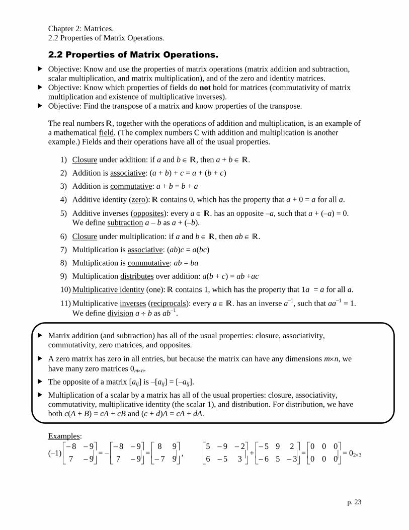
Matrix addition (and subtraction) has all of the usual properties: closure, associativity,
commutativity, zero matrices, and opposites.
A zero matrix has zero in all entries, but because the matrix can have any dimensions mn, we
have many zero matrices 0mn.
The opposite of a matrix [aij] is –[aij] = [–aij].
Multiplication of a scalar by a matrix has all of the usual properties: closure, associativity,
commutativity, multiplicative identity (the scalar 1), and distribution. For distribution, we have
both c(A + B) = cA + cB and (c + d)A = cA + dA.
Examples:
(–1)
97
98= –
97
98=
97
98,
356
295+
356
295=
000
000= 023
Chapter 2: Matrices.
2.2 Properties of Matrix Operations.
p. 24
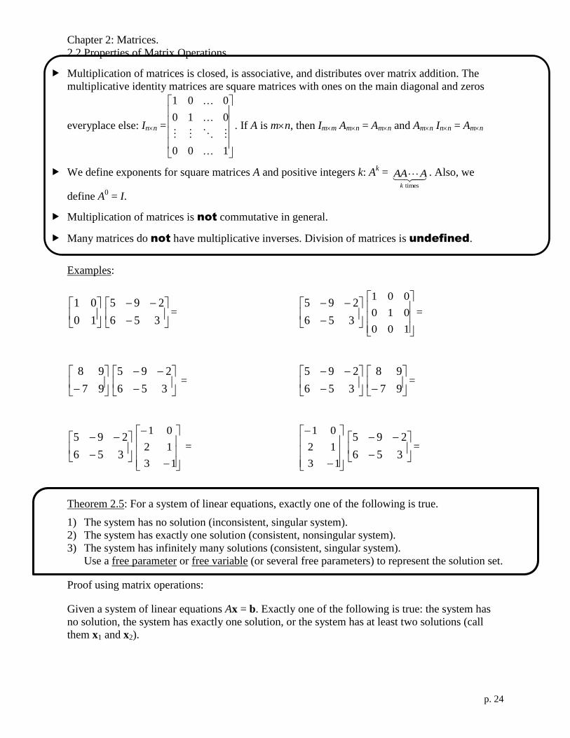
Multiplication of matrices is closed, is associative, and distributes over matrix addition. The
multiplicative identity matrices are square matrices with ones on the main diagonal and zeros
everyplace else: Inn =
100
010
001
. If A is mn, then Imm Amn = Amn and Amn Inn = Amn
We define exponents for square matrices A and positive integers k: Ak =
timesk
AAA . Also, we
define A0 = I.
Multiplication of matrices is not commutative in general.
Many matrices do not have multiplicative inverses. Division of matrices is undefined.
Examples:
10
01
356
295=
356
295
100
010
001
=
97
98
356
295 =
356
295
97
98=
356
295
13
12
01
=
13
12
01
356
295=
Theorem 2.5: For a system of linear equations, exactly one of the following is true.
1) The system has no solution (inconsistent, singular system).
2) The system has exactly one solution (consistent, nonsingular system).
3) The system has infinitely many solutions (consistent, singular system).
Use a free parameter or free variable (or several free parameters) to represent the solution set.
Proof using matrix operations:
Given a system of linear equations Ax = b. Exactly one of the following is true: the system has
no solution, the system has exactly one solution, or the system has at least two solutions (call
them x1 and x2).

Chapter 2: Matrices.
2.2 Properties of Matrix Operations.
p. 25
*
If the system has two solutions, then Ax1 = b and Ax2 = b so
A(x1 – x2) = Ax1 – Ax2 = b – b = 0.
Let xh = x1 – x2, so xh is a nonzero solution to the homogenous equation Ax = 0.
Then for any scalar t, x1 + txh is a solution of Ax = b because
A(x1 + txh) = Ax1 + tAxh = b+ t 0 = b.
Thus, in the last case, the system has infinitely many solutions with a parameter t.
The transpose AT of a matrix A is formed by writing its columns as rows. For example,
if
mnmmm
n
n
n
aaaa
aaaa
aaaa
aaaa
A
321
3333231
2232221
1131211
then
mnnnn
m
m
m
T
aaaa
aaaa
aaaa
aaaa
A
321
3332313
2322212
1312111
.
Equivalently, the transpose of A is formed by writing rows as columns. The ij entry of AT is aji.
Example: Find the transpose of A =
8251
4803
0739
Mathematica: to take the transpose of a matrix, either type Transpose[a] (also available on
the Basic Math Assistant palette) or type a followed by tr (four separate keystrokes).
After the first three keystrokes, you will see atr. After the fourth keystroke, atr will
change to aT. Of course, at the end, type
TI-89: A
MatrixT
Properties of the transpose:
1) (AT)T = A
2) (A + B)T = A
T +B
T
3) (cA) T
=cAT
4) (AB) T
= BTA
T

Chapter 2: Matrices.
2.2 Properties of Matrix Operations.
p. 26
Example of Property #4:
Consider A = and B =
The 32 entry of (AB)T is the 23 entry of AB =
which is a21b13 + a22b23 + a23b33
If we look at AT and B
T, we much reverse the order of multiplication to obtain row column.
BTA
T =
The 32 entry BTA
T is b13a21 + b23a22 + b33a23. You can see that (AB)
T = B
TA
T
A matrix M is symmetric iff MT = M.
Example: M =
525
246
5610
is symmetric. Prove that AAT is symmetric for any matrix A.
Proof:

Chapter 2: Matrices.
2.3 The Inverse of a Matrix.
p. 27
2.3 The Inverse of a Matrix.
Objective: Find the inverse of a matrix (if it exists) by Gauss-Jordan elimination.
Objective: Use properties of inverse matrices.
Objective: Use an inverse matrix to solve a system of linear equations.
A square nn matrix is invertible (or nonsingular) when there exists an nn matrix A–1
such that
AA–1
= Inn and A–1
A = Inn
where Inn is the identity matrix. A–1
is called the (multiplicative) inverse of A. A matrix that does
not have an inverse is called singular (or noninvertible). Nonsquare matrices do not have
inverses.
Theorem 2.7: If A is an invertible matrix, then the inverse is unique.
Proof: let B and C be inverses of A. Then BA = I an AC = I. So
B = BI = B(AC) = (BA)C = IC =C. Therefore, B = C and the inverse of A is unique.
Example: Find the inverse of A =
21
53.
Solution: We need to solve the system AX = I, or
21
53
2221
1211
xx
xx =
10
01,
which gives four equations 121021
053153
22122111
22122111
xxxx
xxxx
To solve these four equations, we take the reduced row echelon forms
021
153
110
201 and
121
053
310
501, so A
–1 = X =
31
52
Since the row operations performed to find the reduced row echelon form depend only on the
coefficient part of the augmented matrix
21
53, we could solve all four equations
simultaneously by using a doubly augmented matrix
[ A | I ] =
1021
0153
3110
5201= [ I | A
–1 ]
To create the doubly augmented matrix in Mathematica from A, type
m=Join[a, IdentityMatrix[2],2]
To create the doubly augmented matrix on the TI-89 from A, type

Chapter 2: Matrices.
2.3 The Inverse of a Matrix.
p. 28
*
Matrix
augment(
A,
Matrix
identity(2))
M
We used IdentityMatrix[2] and identity(2) because we wanted a 22 matrix.
To find the inverse of an nn matrix A by Gauss-Jordan elimination, find the reduced row
echelon form of th n2n augmented matrix [ A | I ]. If the nn block on the left can be reduced to
I, then the nn block on the right is A–1
[ A | I ] [ I | A–1
]
If the nn block on the left cannnot be reduced to I, then A is not invertible.
Example: Invert A =
321
221
111
using Gauss-Jordan elimination.
Example: Invert A =
332
221
111
using Gauss-Jordan elimination.
Example: Invert M =
dc
ba using Gauss-Jordan elimination.
You can also use software. First clear the variables using Clear[a,b,c,d] or
Clear a-z, then type Inverse[m] or
M^1
(also on Basic Math Assistant palette)

Chapter 2: Matrices.
2.3 The Inverse of a Matrix.
p. 29
*
Theorem 2.8 Properties of Inverse Matrices
If A is an invertible matrix, k is a positive integer, and c is a nonzero scalar, then A–1
, Ak, cA, and
AT are invertible, and
1) (A–1
) –1
= A
2) (Ak)–1
= (A–1
)k
3) (cA) –1
= c1 A
–1
4) (AT)–1
= (A–1
)T
Proof:
1)
2) Proof by Induction (see the Appendix)
When k = 1,
If (Ak)–1
= (A–1
)k,
By mathematical induction, we conclude that (Ak)
–1 = (A
–1) for all positive integers k.
3)
4)

Chapter 2: Matrices.
2.3 The Inverse of a Matrix.
p. 30
*
*
*
Theorem 2.9 Inverse of a Product
If A and B are invertible nn matrices, then (AB)–1
= B–1
A–1
.
Proof:
Theorem 2.10 Cancellation Properties
Let C be an invertible matrix.
1) If AC = BC, then A = B. (Right cancellation property)
2) If CA = CB, then A = B. (Left cancellation property)
Theorem 2.11 Systems of Equations with Unique Solutions.
If A is an invertible matrix, then the system Ax = b has a unique solution x = A–1
b.
Review: What is wrong with the following “proof” that if AB = I and CA = I then B = C?
A
CA
A
AB
B = C
What is wrong with the following “proof” that if AB = I and CA = I and A is invertible then B =
C?
AB = CA
A–1
AB = CAA–1
IB = CI
B = C
Chapter 2: Matrices.
2.4 Elementary Matrices.
p. 31
2.4 Elementary Matrices.
Objective: Factor a matrix into a product of elementary matrices.
Objective: Find the PA = LDU factorization of a matrix.
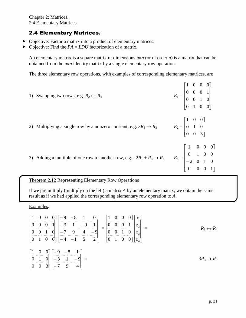
An elementary matrix is a square matrix of dimensions nn (or of order n) is a matrix that can be
obtained from the nn identity matrix by a single elementary row operation.
The three elementary row operations, with examples of corresponding elementary matrices, are
1) Swapping two rows, e.g. R2 R4 E1 =
0010
0100
1000
0001
2) Multiplying a single row by a nonzero constant, e.g. 3R3 R3 E2 =
300
010
001
3) Adding a multiple of one row to another row, e.g. –2R1 + R3 R3 E3 =
1000
0102
0010
0001
Theorem 2.12 Representing Elementary Row Operations
If we premultiply (multiply on the left) a matrix A by an elementary matrix, we obtain the same
result as if we had applied the corresponding elementary row operation to A.
Examples:
0010
0100
1000
0001
2514
9497
1913
0189
=
0010
0100
1000
0001
4
3
2
1
r
r
r
r
= R2 R4
300
010
001
497
913
189
= 3R3 R3

Chapter 2: Matrices.
2.4 Elementary Matrices.
p. 32
1000
0102
0010
0001
2514
9497
1913
0189
= –2R1 + R3 R3
Gaussian elimination can be represented by a product of elementary matrices. For example,
A =
3963
5121
2310
R1 R2 E1 =
100
001
010
3963
2310
5121
3R1+ R3 R3 E2 =
103
010
001
12600
2310
5121
61 R3 R3 E3 =
6/100
010
001
2100
2310
5121
so
2100
2310
5121
= E3(E2(E1A)) =
6/100
010
001
103
010
001
100
001
010
3963
5121
2310
Two nn matrices A and B are row-equivalent when there exist a finite number of elementary
matrices such that B = EnEn–1…E2E1A.

Chapter 2: Matrices.
2.4 Elementary Matrices.
p. 33
A square matrix L is lower triangular if all entries above the main diagonal are zero, i.e. lij = 0
whenever i < j. A square matrix U is upper triangular if all entries below the main diagonal are
zero, i.e. uij = 0 whenever i > j. A square matrix D is diagonal if all entries not on the main
diagonal are zero, i.e. dij = 0 whenever i j.
L =
0
00
U =
00
0 D =
00
00
00
Theorem 2.13+ Elementary Matrices are Invertible
If E is an elementary matrix, then E–1
exists and is an elementary matrix. Moreover, if E is lower
triangular, then E–1
is also lower triangular. And if E is diagonal, then E–1
is also diagonal.
Examples:
E1 =
100
001
010
R1 R2 E1–1
=
100
001
010
R1 R2
E2 =
103
010
001
3R1+ R3 R3 E2–1
=
103
010
001
–3R1+ R3 R3
E3 =
6/100
010
001
61 R3 R3 E3
–1 =
600
010
001
6R3 R3
You can check these using matrix multiplication.
E.g.
103
010
001
103
010
001
=
100
010
001
and
103
010
001
103
010
001
=
100
010
001
.
Theorem 2.14 Invertible Matrices are Row-Equivalent to the Identity Matrix
A square matrix A is invertible if and only if it is row equivalent to the identity matrix:
A = En…E2E1I = En…E2E1
if and only if A is a product of elementary matrices.
Proof of “If A is invertible, then A is a product of elementary matrices”:
Since A is invertible, Ax = b has a unique solution (namely, x = A–1
b). But this means that we
can use row operations to reduce [ A | b ] to [ I | c ] (where c = A–1
b, of course). If the

Chapter 2: Matrices.
2.4 Elementary Matrices.
p. 34
corresponding elementary matrices are E1, E2, …, En, then I = EnEn–1…E2E1A so
A = E1–1
E2–1
… En–1–1
En–1
, which is a product of elementary matrices.
Proof of “If A is a product of elementary matrices, then A is invertible”:
If A = E1E2… En–1En, then A–1
exists and A–1
= En–1
En–1–1
…E2–1
E1–1
because every elementary
matrix is invertible.-
Theorem 2.15 Equivalent Conditions for Invertibility
If A is an n n matrix, then the following statements are equivalent.
1) A is invertible.
2) Ax = b has a unique solution for every n1 column matrix b (namely, x = A–1
b).
3) Ax = 0 has only the trivial solution.
4) A is row-equivalent to Inn.
5) A can be written as a product of elementary matrices.
Returning to our example of Gaussian elimination using elementary matrices, we found the
reduced echelon form of the augmented matrix
3963
5121
2310
2100
2310
5121
=
6/100
010
001
103
010
001
100
001
010
3963
5121
2310
Look just at the 33 coefficient matrix instead of the 34 augmented matrix. We have
U
formechelon -row
100
310
121
=
mRows
6/100
010
001
mRowAdds
103
010
001
swaps row
100
001
010
A
963
121
310
The row-echelon form is upper triangular. In general, we may have more than one mRow
(multiply a row by a nonzero constant) elementary matrix, more than one mRowAdd (add a
multiple of one row to another row) elementary matrix, and more than one row swap matrix. The
product of and arbitrary number of row swap matrices is called a permutation matrix P.
U=
mRows
12 FFFn
mRowAdds
12 EEEm PA
Chapter 2: Matrices.
2.4 Elementary Matrices.
p. 35
ngularlower tria
mRowAdds
11
2
1
1
mEEE
diagonal
mRows
11
2
1
1
nFFF U= PA
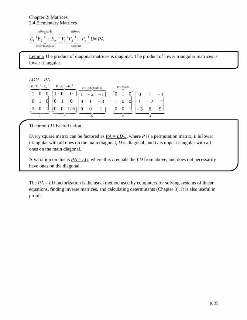
Lemma The product of diagonal matrices is diagonal. The product of lower triangular matrices is
lower triangular.
LDU = PA
L
EEE m11
21
1
103
010
001
D
FFF n11
21
1
6/100
010
001
U
formechelon -row
100
310
121
=
P
swaps row
100
001
010
A
963
121
310
Theorem LU-Factorization
Every square matrix can be factored as PA = LDU, where P is a permutation matrix, L is lower
triangular with all ones on the main diagonal, D is diagonal, and U is upper triangular with all
ones on the main diagonal.
A variation on this is PA = LU, where this L equals the LD from above, and does not necessarily
have ones on the diagonal.
The PA = LU factorization is the usual method used by computers for solving systems of linear
equations, finding inverse matrices, and calculating determinants (Chapter 3). It is also useful in
proofs.

Chapter 2: Matrices.
2.4 Elementary Matrices.
p. 36
*
Example: Find the PA = LDU factorization of A =
632
101
110
Solution: A =
632
101
110
21 RR
632
110
101
3312 RRR
430
110
101
3323 RRR
100
110
101
22 RR
100
110
101
= U
U
100
110
101
=
F
100
010
001
2
130
010
001
E
1
102
010
001
E
P
100
001
010
A
632
101
110
1
1
102
010
001
E
1
2
130
010
001
E
1
100
010
001
F
U
100
110
101
=
P
100
001
010
A
632
101
110
L
132
010
001
D
100
010
001
U
100
110
101
=
P
100
001
010
A
632
101
110

Chapter 2: Matrices.
2.5 Applications of Matrix Operations.
p. 37
drop
A B
*
2.5 Applications of Matrix Operations.
Objective: Write and use a stochastic (Markov) matrix.
Objective: Use matrix multiplication to encode and decode messages.
Objective: Use matrix algebra to analyze and economic system (Leontief input-output model).
Consider a situation in which members of a population occupy a finite number of states {S1, S2,
…, Sn}. For example, a multinational company has $4 trillion in assets (the population). Some of
the money is in the Americas, some in Asia, and the rest is in Europe (the three states). In a
Markov process, at each discrete step in time, members of the population may move from one
state to another, subject to the following rules:
1) The total number of individuals stays the same.
2) The numbers in each state never become negative.
3) The new state depends only on the current state (history is disregarded).
The behavior of a Markov process is described by a matrix
of transition probabilities (or stochastic matrix or Markov
matrix).
pij is the probability that a member of the population will
change from the j th
state to the i th
state. The rules above
become
1) Each column of the transition matrix adds up to one.
2) Every probability entry is 0 ≤ pij ≤ 1.
Example: Stochastic Matrix. A chemistry course is taught in two sections. Every week,41 of the
students in Section A and31 of the students in Section B drop, and
61 of each section transfer to
the other section. Write the transition matrix. At the beginning of the semester, each section has
144 students. Find the number of students in each section and the number of students who have
dropped after one week and after two weeks.
Solution:
P =
1
01
01
31
41
31
61
61
61
61
41
(d)
(B)
(A)
=
1
0
0
31
41
21
61
61
127
.
P
0
144
144
=
84
96
108
(d)
(B)
(A)
. P
84
96
108
=
143
66
79
(d)
(B)
(A)
to
from
2
1
21
22221
11211
21
nnnnn
n
n
n
S
S
S
ppp
ppp
ppp
P
SSS
61
61
31
004
1
127
21
1
61
Chapter 2: Matrices.
2.5 Applications of Matrix Operations.
p. 38
*--
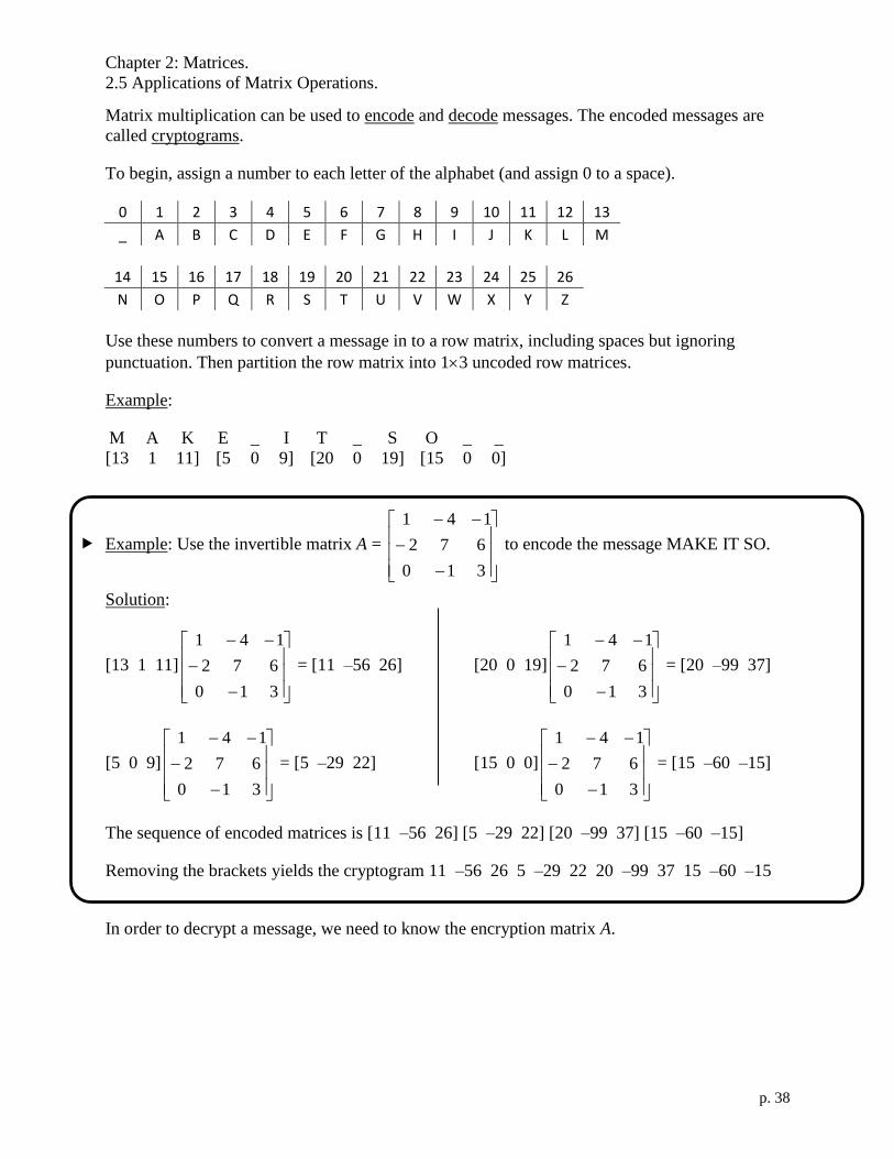
Matrix multiplication can be used to encode and decode messages. The encoded messages are
called cryptograms.
To begin, assign a number to each letter of the alphabet (and assign 0 to a space).
0 1 2 3 4 5 6 7 8 9 10 11 12 13
_ A B C D E F G H I J K L M
14 15 16 17 18 19 20 21 22 23 24 25 26
N O P Q R S T U V W X Y Z
Use these numbers to convert a message in to a row matrix, including spaces but ignoring
punctuation. Then partition the row matrix into 13 uncoded row matrices.
Example:
M A K E _ I T _ S O _ _
[13 1 11] [5 0 9] [20 0 19] [15 0 0]
Example: Use the invertible matrix A =
310
672
141
to encode the message MAKE IT SO.
Solution:
[13 1 11]
310
672
141
= [11 –56 26] [20 0 19]
310
672
141
= [20 –99 37]
[5 0 9]
310
672
141
= [5 –29 22] [15 0 0]
310
672
141
= [15 –60 –15]
The sequence of encoded matrices is [11 –56 26] [5 –29 22] [20 –99 37] [15 –60 –15]
Removing the brackets yields the cryptogram 11 –56 26 5 –29 22 20 –99 37 15 –60 –15
In order to decrypt a message, we need to know the encryption matrix A.

Chapter 2: Matrices.
2.5 Applications of Matrix Operations.
p. 39
*-–-
Example: Use the invertible matrix A =
310
672
141
to decode
–8 26 31 13 –73 50 19 –97 44 16 –64 –16.
Solution:
A–1
=
112
436
171327
[–8 26 31]
112
436
171327
= [2 5 1] [19 –97 44]
112
436
171327
= [19 0 21]
[13 –73 50]
112
436
171327
= [13 0 21] [16 –64 –16]
112
436
171327
= [16 0 0]
[2 5 1] [13 0 21] [19 0 21] [16 0 0]
B E A M _ U S _ U P _ _
In economics, an input-output model (developed by
Leontief) consists of n different industries In, each of
which needs inputs (e.g. steel, food, labor, …) and has
and output. To produce a unit (e.g. $1 million) of output,
an industry may use the outputs of other industries and of
itself. For example, production of steel may use steel,
food, and labor.
Let dij be the amount of output the industry j needs from industry i to produce one unit of output
per year. (We assume the dij are constant, i.e. fixed prices.) The matrix of these coefficients is
called the input-output matrix or consumption matrix D. A column represents all of the inputs to
a given industry. For this model to work, 0 ≤ dij ≤ 1 and the sum of the entries in each column
must be less than or equal to 1. (Otherwise, it costs more than one unit to produce a unit in that
industry.)
Let xi be the total output matrix of industry i, and X = [xi]. If the economic system is closed (self-
sustaining: total output = “intermediate demand,” i.e. what is needed to produce it), then X = DX.
If the system is open with external demand matrix E (e.g. exports) then X = DX + E.
To find what output matrix is needed to produce a given external demand matrix, we solve
(Input)
Supplier
(Output)User
2
1
21
22221
11211
21
nnnnn
n
n
n
I
I
I
ddd
ddd
ddd
D
III
Chapter 2: Matrices.
2.5 Applications of Matrix Operations.
p. 40
*-–-
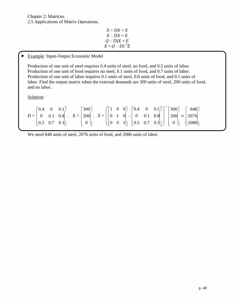
X = DX + E
X – DX = E
(I – D)X = E
X = (I – D)–1
E
Example: Input-Output Economic Model
Production of one unit of steel requires 0.4 units of steel, no food, and 0.5 units of labor.
Production of one unit of food requires no steel, 0.1 units of food, and 0.7 units of labor.
Production of one unit of labor requires 0.1 units of steel, 0.8 units of food, and 0.1 units of
labor. Find the output matrix when the external demands are 300 units of steel, 200 units of food,
and no labor.
Solution:
D =
1.07.05.0
8.01.00
1.004.0
. E =
0
200
300
. X =
1
1.07.05.0
8.01.00
1.004.0
100
010
001
0
200
300
2086
2076
848
We need 848 units of steel, 2076 units of food, and 2086 units of labor.

Chapter 3: Determinants.
3.1 The Determinant of a Matrix.
p. 41
Chapter 3: Determinants.
3.1 The Determinant of a Matrix.
Objective: Find the determinant of a 22 matrix.
Objective: Find the minors and cofactors of a matrix.
Objective: Use expansion by cofactors to find the determinant of a matrix.
Objective: Find the determinant of a triangular matrix.
Every square matrix can be associated with a scalar called its determinant. Historically,
determinants were recognized as a pattern of nn systems of linear equations. The system
2222121
1212111
bxaxa
bxaxa
has the solution
21122211
2122211
aaaa
baabx
and
21122211
2112112
aaaa
abbax
.
The determinant of a 11 matrix A = 11a is det(A) = |A| = a11. The |…| symbols mean
determinant, not absolute value.
The determinant of a 22 matrix A =
2221
1211
aa
aa is det(A) = |A| =
2221
1211
aa
aa = a11a22 – a12a21.
Geometrically, the signed area
of a parallelogram with
vertices at (0, 0), (x1, y1), (x2,
y2), and (x1 + x2, y1 + y2) is
A = 22
11
yx
yx
(The area is positive if the angle from
(x1, y1) to (x2, y2) is counterclockwise;
otherwise, the area is negative.)
Proof:
The area A of the parallelogram is
A = area of large rectangle areas of four triangles areas of two small rectangles
= (x1 + x2)(y1 + y2) 21 x1y1
21 x1y1
21 x2y2
21 x2y2 2x2y1
= x1y1 + x1y2 + x2y1 + x2y2 x1y1 x2y2 2x2y1
= x1y2 x2y1 = 22
11
yx
yx
(x2, y2)
(x1, y1)

Chapter 3: Determinants.
3.1 The Determinant of a Matrix.
p. 42
To define the determinant of a square matrix A of order (dimensions) higher than 2, we define
minors and cofactors. The minor Mij of the entry aij is the determinant of the matrix obtained by
deleting row i and column j of A. The cofactor Cij of the entry aij is Cij = (–1)i+j
Mij. Notice that
(–1)i+j
is a “checkerboard” pattern: (–1)i+j
=
Examples: Finding Cofactors. Let A =
Find C21. Solution: C21 = –3332
1312
aa
aa = –a12a33 + a13a32
Find C22. Solution: C22 = +3331
1311
aa
aa = a11a33 – a13a31
The determinant of an nn matrix A (n ≥ 2) is the sum of the entries in the first row of A
multiplied by their respective cofactors.
det(A) =
n
j
jjCa1
11 = a11C11 + a12C12 + … + a1nC1n
Example:
953
786
433
= 395
78
+ 3
93
76 + 4
53
86
= 3(–72 – 35) +3(54 – 21) + 4(30 + 24) = 3(–107) +3(33) +4(54) = –6
Theorem 3.1 Expansion by Cofactors
Let A be a square matrix of order n. Then the determinant of A is given by an expansion in any
row i
det(A) =
n
j
ijijCa1
= ai1Ci1 + ai2Ci2 + … + ainCin
and also by an expansion in any column j
det(A) =
n
i
ijijCa1
= a1jC1j + a2jC2j + … + anjCnj

Chapter 3: Determinants.
3.1 The Determinant of a Matrix.
p. 43
When expanding, you don’t need to find the cofactors of zero entries, because aijCij = (0)Cij = 0.
The definition of the determinant is inductive, because it uses the determinant of a matrix of
order n – 1 to define the determinant of a matrix of order n.
Example: Expanding by Cofactors to Find a Determinant
= = –1 + 3(– )
= –1(2 +7 ) +3(–2 ) = –1(2(3) + 7(–6)) + 3(–2)(0) = –(6 – 42) = 36
To find a determinant using Mathematica, type Det[a]
(also on Basic Math Assistant, More drop-down menu)
To find a determinant on the TI-89, type
Matrix
det(
A
To find a determinant of a 33 matrix, you can also use the following shortcut. Copy Columns 1
and 2 into Columns 4 and 5. To calculate the determinant, add and subtract the indicated
products.
333231
232221
131211
aaa
aaa
aaa
3231
2221
1211
333231
232221
131211
aa
aa
aa
aaa
aaa
aaa
333231
232221
131211
aaa
aaa
aaa
= a11a22a33 + a12a23a31 + a13a21a32 – a31a22a13 – a32a23a11 – a33a21a12
Example:
851
640
311
51
40
11
851
640
311
so
851
640
311
= 32 + 6 + 0 – 12 – 30 – 0 = –4
subtract
add
32 6 0
12 30 0
Chapter 3: Determinants.
3.1 The Determinant of a Matrix.
p. 44
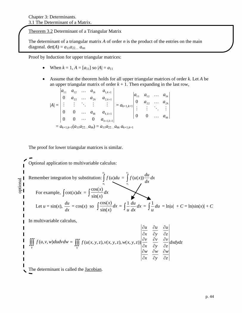
Theorem 3.2 Determinant of a Triangular Matrix
The determinant of a triangular matrix A of order n is the product of the entries on the main
diagonal. det(A) = a11a22… ann
Proof by Induction for upper triangular matrices:
When k = 1, A = [a11] so |A| = a11
Assume that the theorem holds for all upper triangular matrices of order k. Let A be
an upper triangular matrix of order k + 1. Then expanding in the last row,
|A| =
1,1
1,
1,2222
1,111211
000
00
0
kk
kkkk
kk
kk
a
aa
aaa
aaaa
= ak+1,k+1
kk
k
k
a
aa
aaa
00
0 222
11211
= ak+1,k+1(a11a22…akk) = a11a22…akk ak+1,k+1
The proof for lower triangular matrices is similar.
Optional application to multivariable calculus:
Remember integration by substitution: 2
1
)(
u
u
duuf = 2
1
))((
x
x
dxdx
duxuf
For example, dxx)cot( = dxx
x
)sin(
)cos(
Let u = sin(x), dx
du = cos(x) so dx
x
x
)sin(
)cos( = dx
dx
du
u
1 = du
u
1 = ln|u| + C = ln|sin(x)| + C
In multivariable calculus,
V
dudvdwwvuf ),,( =
V
dxdydz
z
w
y
w
x
w
z
v
y
v
x
v
z
u
y
u
x
u
zyxwzyxvzyxuf )),,(),,,(),,,((
The determinant is called the Jacobian.
opti
onal

Chapter 3: Determinants.
3.2 Determinants and Elementary Operations.
p. 45
3.2 Determinants and Elementary Operations.
Objective: Use elementary row operations to evaluate a determinant.
Objective: Use elementary column operations to evaluate a determinant.
Recognize conditions that yield zero determinants.
In practice, we rarely evaluate determinants using expansion by cofactors. The properties of
determinants under elementary operations provide a much quicker way to evaluate determinants.
Theorem 3.9 det(AT) = det(A). [Proof is in Section 3.4]
Theorem 3.3 Elementary Row (Column) Operations and Determinants.
Let A and B be nn square matrices.
a) When B is obtained from A by swapping two rows (two columns) of A, det(B) = –det(A).
b) When B is obtained from A by adding a multiple of one row of A to another row of A (or one
column of A to another column of A), det(B) = det(A).
c) When B is obtained from A by multiplying of a row (column) of A by a nonzero constant c,
det(B) = c det(A).
Theorem 3.4 Conditions that Yield a Zero Determinant.
If A is an nn square matrix and any one of the following conditions is true, then det(A) = 0
a) An entire row (or an entire column) consists of zeros.
b) Two rows (or two columns) are equal.
c) One row is a multiple of another row (or one column is a multiple of another column).
Proof by Induction of 3.3a (for rows):
When k = 2, A =
2221
1211
aa
aa and B =
1211
2221
aa
aa so
det(B) = a21a12 – a22a11 = –(a11a22 – a12a21) = –det(A)
Assume that the theorem holds for all matrices of order k. Let A be a matrix of order k
+ 1 and B be a matrix obtained by swapping two rows of A. To find det(A) and det(B),
expand in any row other than the swapped rows. The respective cofactors are
opposites, because they come from kk matrices that have two rows swapped. Thus,
det(B) = –det(A).
Proof of 3.4a (for rows): Suppose that row i of A is all zeroes. Expand by cofactors in row i.
det(A) =
n
j
ijijCa1
=
n
j
ijC1
0 = 0

Chapter 3: Determinants.
3.2 Determinants and Elementary Operations.
p. 46
Proof of 3.4b: Let B be the matrix obtained from A by swapping the two identical rows
(columns) of A, so det(B) = –det(A). But B = A, so det(A) = –det(A) so det(A) = 0.
Proof of 3.3b (for rows): Suppose B is obtained from A by adding c times row k to row i. Expand
by cofactors in row i. Note that the cofactors of Cij are the same for matrices A and B,
because the matrices are the same everywhere except row i.
det(B) =
n
j
ijijCb1
=
n
j
ijijkj Caca1
)( =
n
j
ijkjCac1
+
n
j
ijijCa1
= c·0 + det(A) = det(A).
because
n
j
ijkjCa1
is the determinant of a matrix with two identical rows (row k and row i).
See Theorem 3.4b.
Another way of writing this is
nnn
inknik
knk
n
aa
acaaca
aa
aa
1
11
1
111
)()(
= c
nnn
knk
knk
n
aa
aa
aa
aa
1
1
1
111
+
nnn
ini
knk
n
aa
aa
aa
aa
1
1
1
111
= c·0 + det(A) = det(A).
Proof of 3.3c (for rows): Suppose B is obtained from A by multiplying row i by a nonzero scalar
c. Expand by cofactors in row i.
det(B) =
n
j
ijijCb1
=
n
j
ijijCca1
= c
n
j
ijijCa1
= c det(A)
Proof of 3.4c: Suppose B is a matrix with two equal rows (or two equal columns), and A is
obtained from B by multiplying one of those rows (or columns) by a nonzero scalar c. Using
3.3c on that row (or column), det(A) = c det(B). Using 3.4b, det(B) = 0. Thus, det(A) = 0.
Geometrically, the signed area of a parallelogram with edges from
(0, 0) to (x1, y1) and from (0, 0) to (x2, y2) has the same properties
as 22
11
yx
yx when you perform an elementary row operation. Also,
the signed area of a parallelepiped with edges from (0, 0) to (x1, y1,
z1), from (0, 0) to (x2, y2, z2), and from (0, 0) to (x3, y3, z3) has the
same properties as
333
222
111
zyx
zyx
zyx
when you perform an elementary
row operation.
Chapter 3: Determinants.
3.2 Determinants and Elementary Operations.
p. 47
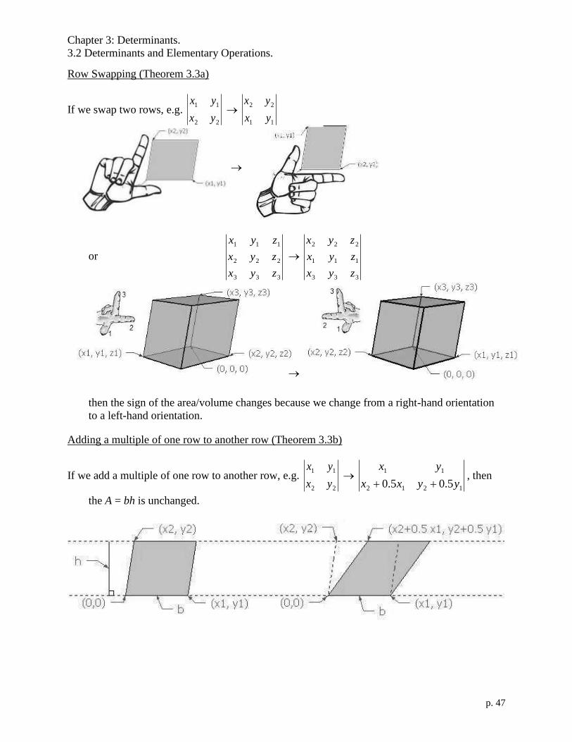
Row Swapping (Theorem 3.3a)
If we swap two rows, e.g. 22
11
yx
yx
11
22
yx
yx
or
333
222
111
zyx
zyx
zyx
333
111
222
zyx
zyx
zyx
then the sign of the area/volume changes because we change from a right-hand orientation
to a left-hand orientation.
Adding a multiple of one row to another row (Theorem 3.3b)
If we add a multiple of one row to another row, e.g. 22
11
yx
yx
1212
11
5.05.0 yyxx
yx
, then
the A = bh is unchanged.
Chapter 3: Determinants.
3.2 Determinants and Elementary Operations.
p. 48
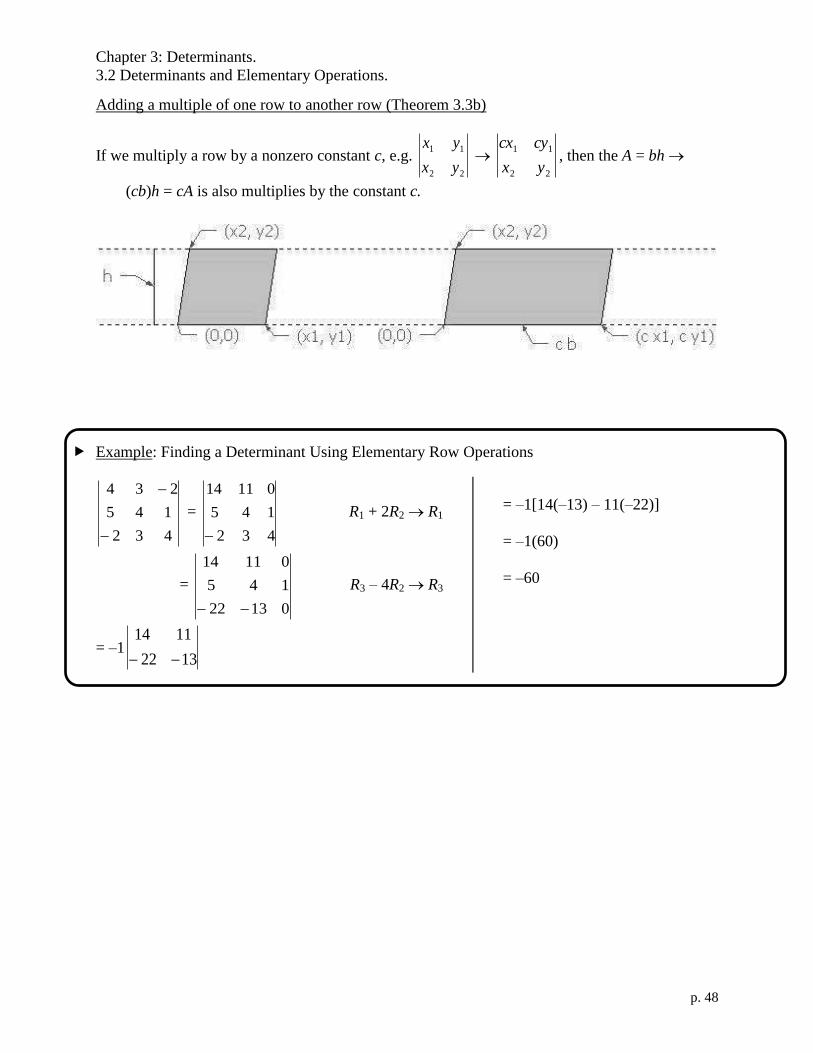
Adding a multiple of one row to another row (Theorem 3.3b)
If we multiply a row by a nonzero constant c, e.g. 22
11
yx
yx
22
11
yx
cycx, then the A = bh
(cb)h = cA is also multiplies by the constant c.
Example: Finding a Determinant Using Elementary Row Operations
432
145
234
=
432
145
01114
R1 + 2R2 R1
=
01322
145
01114
R3 – 4R2 R3
= –11322
1114
= –1[14(–13) – 11(–22)]
= –1(60)
= –60

Chapter 3: Determinants.
3.2 Determinants and Elementary Operations.
p. 49
Example: Finding a Determinant Using Elementary Column Operations
2159
3157
5642
4331
=
______9
______7
______2
0001
44
33
212
____
____
3
CC
CC
CCC
= (__)
______9
______7
____12
0001
22___ CC
= (__)
______9
______7
0012
0001
4
3
__________
__________
C
C
= (__)(__) ______
______
001
= (__)(__)(__) ____
____
=


Chapter 3: Determinants.
3.3 Properties of Determinants.
p. 51
3.3 Properties of Determinants.
Objective: Find the determinant of a matrix product and of a scalar multiple of a matrix.
Find the determinant of an inverse matrix and recognize equivalent conditions for a nonsingular
matrix.
Find the determinant of the transpose of a matrix.
Theorem 3.5 Determinant of a Matrix Product
If A and B are square matrices of the same order, then det(AB) = det(A) det(B).
Proof: To begin, let E be an elementary matrix. By Thm 2.12, EB is the matrix obtained from
applying the corresponding row operation to B. By Thm. 3.3,
det(EB) =
)det(
)det(
)det(
Bc
B
B
if the row operation is
cconstant nonzero aby row a gmultiplyin
another torow one of multiple a adding
rows twoexchanging
Also by Thm 3.3,
det(E) = det(EI) =
c
1
1
if the row operation is
cconstant nonzero aby row a gmultiplyin
another torow one of multiple a adding
rows twoexchanging
Thus, det(EB) = det(E) det(B). This can be generalized by induction to conclude that
|Ek…E2E1B| = |Ek| |…| |E2| |E1| |B| where the Ei are elementary matrices. If A is nonsingular,
then by Thm. 2.14, it can be written as the product A = Ek…E2E1 so |AB| = |A| |B|.
If A is singular, then A is row-equivalent to a matrix with an entire row of zeroes (for example,
the reduced row echelon form). From Thm 3.4, we know |A| = 0. Moreover, because A is
singular, it follows that AB must be singular. (Proof by contradiction: if AB were nonsingular,
then A[B(AB)-1
] = I would show that A is not singular, because A–1
= B(AB)-1
.) Therefore, |AB|
= 0 = |A| |B|.
Comment on Proof by Contradiction: “P implies Q” is equivalent to “not Q implies not P.”
Theorem 3.6 Determinant of a Scalar Multiple of a Matrix
If A is a square matrix of order n and c is a scalar, then det(cA) = cndet(A).
Proof: Apply Property (c) of Thm. 3.3 to each of the n rows of A to obtain n factors of c.
Theorem 3.7 Determinant of an Invertible Matrix
A square matrix A is invertible (nonsingular) if and only if det(A) 0.
Proof: On the one hand, if A is invertible, then AA–1
= I, so . |A| |A–1
| = | I | = 1. Therefore, |A| 0.
On the other hand, assume det(A) 0. Then use Gauss-Jordan elimination to find the reduced
row-echelon form R. Since R is in reduced row-echelon form, it is either the identity matrix or

Chapter 3: Determinants.
3.3 Properties of Determinants.
p. 52
it must have at least one row of all zeroes. The second case is not possible: if R had a row of all
zeroes, then det(R) = 0, but then det(A) = 0 (which contradicts the assumption). Therefore, A is
row-equivalent to R = I, so A is invertible.
Theorem 3.8 Determinant of an Inverse Matrix
If A is an invertible matrix, then det (A–1
) = )det(
1
A
Proof: AA–1
= I, so . |A| |A–1
| = | I | = 1 and |A| 0, so |A–1
| =||
1
A.
Equivalent Conditions for a Nonsingular nn Matrix (Summary)
1) A is invertible.
2) Ax = b has a unique solution for every n1 column matrix b.
3) Ax = 0 has only the trivial solution for the n1 column matrix 0.
4) A is row-equivalent to I.
5) A can be written as a product of elementary matrices.
6) det(A) 0.
Theorem 3.9 Determinant of a the Transpose of a Matrix
If A is a square matrix, then det(AT) = det(A).
Proof: Let A be a square matrix of order n.
From Section 2.4, we know that A can be factored as PA = LDU, where P is a permutation
matrix, L is lower triangular with all ones on the main diagonal, D is diagonal, and U is upper
triangular with all ones on the main diagonal.
L is obtained from I by adding a multiple of the rows containing the diagonal ones to the rows
below the diagonal, so
|L| = |I | = 1
by Thm. 3.3b. Likewise, U is obtained from I by adding a multiple of the rows containing the
diagonal ones to the rows above the diagonal, so
|U| = |I | = 1
by Thm. 3.3b.
By Thm. 3.2,
|D| = d11d22… dnn
i.e. the product of its diagonal elements.
P is a product of elementary row-swap matrices, each of which has determinant –1. So |P| is
the product of some number of –1’s.
|P| = 1 if the number of row swaps is even;
|P| = –1 if the number of row swaps is odd.

Chapter 3: Determinants.
3.3 Properties of Determinants.
p. 53
Let e1 =
0
0
1
, e2 =
0
1
0
, …, en =
1
0
0
be n1 matrices. Then P =
T
i
T
i
T
i
ne
e
e
2
1
where i1, i2, …, in is
some permutation of 1, 2, …, n. Now PT =
niii eee 21
, so
PPT =
nnnn
n
n
i
T
ii
T
ii
T
i
i
T
ii
T
ii
T
i
i
T
ii
T
ii
T
i
eeeeee
eeeeee
eeeeee
21
22212
12111
=
100
010
001
= I,
and by Thm. 3.5, det(P) det(PT
) = det(PPT
) = det(I) = 1.
Then either det(P) = 1 so det(PT) = 1, or det(P) = –1 so det(P
T) = –1. In both cases,
det(P) = det(PT).
So we have PA = LDU which gives us |P| |A| = |L| |D| |U| = (1) |D| (1) =|D|, so
|A| = ||
||
P
D.
Taking the transpose, we have ATP
T = U
TD
TL
T which gives us |A
T| |P
T| = |U
T| |D
T| |L
T|.
Now |PT| = |P|; |D
T| = |D| because
DT = D
since D is diagonal;
|LT| = 1
because LT is upper triangular with all ones on the main diagonal; and
|UT| = 1
because UT is lower triangular with all ones on the main diagonal.
Thus, |AT| |P
T| = |U
T| |D
T| |L
T| becomes |A
T| |P
T| = (1) |D| (1), so
|AT| =
||
||TP
D =
||
||
P
D = |A|.

Chapter 3: Determinants.
3.4 Applications of Determinants.
p. 55
3.4 Applications of Determinants.
Objective: Find the adjoint of a matrix and use it to find the inverse of a matrix.
Objective: Use Cramer’s Rule to solve a system of n linear equations in n unknowns.
Objective: Use determinants to find area, volume, and the equations of lines and planes.
Using the adjoint of a matrix to calculate the inverse is time-consuming and inefficient. In
practice, Gauss-Jordan elimination is used for 33 matrices and larger. However, “adjoint” is
vocabulary you may be expected to know in future classes.
Recall from Section 3.1 that the cofactor Cij of a matrix A is (–1)i+j
times the determinant of the
matrix obtained by deleting row i and column j of A.
The matrix of cofactors of A is
nnnn
n
n
CCC
CCC
CCC
21
22221
11211
.
The adjoint of A is the transpose of matrix of cofactors: adj(A) =
nnnn
n
n
CCC
CCC
CCC
21
22212
12111
Theorem 3.10 The Inverse of a Matrix Given by Its Adjoint
If A is an invertible matrix, then A–1
=)det(
1
Aadj(A).
Proof: Consider A[adj(A)] =
nnnn
kiii
n
n
aaa
aaa
aaa
aaa
21
21
22221
11211
nnjnnn
nj
nj
CCCC
CCCC
CCCC
21
222212
112111
The ij entry of this product is ai1Cj1 + ai2Cj2 + … + ainCjn.
If i = j, this is det(A) (expanded by cofactors in row i). If i j, this is the determinant of the
matrix B, which is the same as A except that row j has been replaced with row i.
opti
onal
Chapter 3: Determinants.
3.4 Applications of Determinants.
p. 56
A =
nnnn
jnjj
kiii
n
n
aaa
aaa
aaa
aaa
aaa
21
21
21
22221
11211
, B[adj(A)] =
nnnn
inii
kiii
n
n
aaa
aaa
aaa
aaa
aaa
21
21
21
22221
11211
nnjnnn
nj
nj
CCCC
CCCC
CCCC
21
222212
112111
The j column of the cofactor matrix is unchanged, because it does not depend on the j row of A
or B. Since two rows of B are the same, the cofactor expansion for i j is zero.
Thus, A[adj(A)] =
)det(00
0)det(0
00)det(
A
A
A
= det(A)I.
det(A) 1 because A is invertible, so we can write A[)det(
1
Aadj(A)] = I, so A
–1 =
)det(
1
Aadj(A).
For 33 matrices and larger, Gauss-Jordan elimination is much more efficient than the adjoint
method for finding the inverse of a matrix.
However, for a 22 matrix A =
dc
ba, adj(A) =
ac
bd so A
–1 =
bcad
1
dc
ba.
Cramer’s Rule to solve n linear equation in n variables is time-consuming and inefficient. In
practice, Gaussian elimination is used to solve linear systems. However, Cramer’s Rule is
vocabulary you may be expected to know in future classes.
Theorem 3.11 Cramer’s Rule
If an nn system Ax = b has a coefficient matrix with nonzero determinant |A| 0, then
)det(
)det( 11
A
Ax ,
)det(
)det( 22
A
Ax , …
)det(
)det(
A
Ax n
n
where Ai is the matrix A but with column i replace by b.

Chapter 3: Determinants.
3.4 Applications of Determinants.
p. 57
Proof:
nx
x
x
2
1
x = A–1
b = )det(
1
Aadj(A)b =
)det(
1
A
nnnn
n
n
CCC
CCC
CCC
21
22212
12111
nb
b
b
2
1
so xi = )det(
1
A(b1C1i + b2C2i + … + bnCni). The sum in parentheses is the cofactor expansion of
det(Ai), so xi = )det(
)det(
A
Ai
Example: Solve 1543
1021
yx
yx using Cramer’s Rule.
Solution: x =
43
21
415
210
= 2
10
= –5; y =
43
21
153
101
= 2
15
=
2
15
Area, Volume and Equations of Lines and Planes:
We already know that the signed area of a parallelogram
is given by a 22 determinant (Section 3.1). A = 22
11
yx
yx
The signed area of a triangle with vertices (x1, y1), (x2, y2), and (x3, y3) is A =
1
1
1
33
22
11
yx
yx
yx
Proof:
The area of a triangle is half of the area of a
parallelogram. So the area of the triangle we want is
21
pos
33
22
yx
yx+
21
neg
11
33
yx
yx+
21
neg
22
11
yx
yx=
1
1
1
2
1
33
22
11
yx
yx
yx
For a triangle the signed area is A =
1
1
1
2
1
33
22
11
yx
yx
yx
If the vertices (x1, y1), (x2, y2), and (x3, y3) are ordered clockwise then the area is positive;
otherwise, it is negative. (The homework asks for the absolute value of the area.)
(x2, y2) (x1, y1)
(x3, y3)

Chapter 3: Determinants.
3.4 Applications of Determinants.
p. 58
The area of the triangle is zero if and only if the three points are collinear.
(x1, y1), (x2, y2), and (x3, y3) are collinear if and only if
1
1
1
33
22
11
yx
yx
yx
= 0
The equation of a line through distinct points (x1, y1) and (x2, y2) is
1
1
1
22
11
yx
yx
yx
= 0
Similarly to the two-dimensional case of a parallelogram,
the signed volume of a parallelepiped is given
by a 33 determinant (Section 3.1). V =
333
222
111
zyx
zyx
zyx
Let’s find the volume of the tetrahedron (pyramid with four triangular faces) with vertices at
(x1, y1, z1), (x2, y2, z2), (x3, y3, z3), and (x4, y4, z4).
The volume of the tetrahedron with vertices at (0, 0, 0), (x1, y1, z1), (x2, y2, z2), and (x3, y3, z3) is 61
times the volume of the parallelepiped, i.e.
333
222
111
6
1
zyx
zyx
zyx
. For the triangle above
(21
1
1
1
33
22
11
yx
yx
yx
), we had 3 sides and the areas of 3 triangles to add/subtract. Now we have 4faces
and the volumes of 4 tetrahedrons to add/subtract. The signed volume of the tetrahedron with
vertices at (0, 0, 0), (x1, y1, z1), (x2, y2, z2), and (x3, y3, z3) is (imagine for the moment that (x4, y4,
z4) in front of the triangle (x1, y1, z1), (x2, y2, z2), (x3, y3, z3)
V =
333
444
111
6
1
zyx
zyx
zyx
+
222
211
444
6
1
zyx
zyx
zyx
+
444
333
222
6
1
zyx
zyx
zyx
+
111
222
333
6
1
zyx
zyx
zyx
For a tetrahedron, the signed volume is
V = –
1
1
1
1
6
1
444
333
222
111
zyx
zyx
zyx
zyx

Chapter 3: Determinants.
3.4 Applications of Determinants.
p. 59
If when you wrap the fingers of your right from
(x1, y1, z1) to (x2, y2, z2) to (x3, y3, z3), your thumb points
toward (x4, y4, z4), then the signed volume is positive.
If when you wrap the fingers of your left from (x1, y1, z1)
to (x2, y2, z2) to (x3, y3, z3), your thumb points toward
(x4, y4, z4), then the signed volume is negative.
(The homework asks for the absolute value of the
volume.)
Four points (x1, y1, z1), (x2, y2, z2), (x3, y3, z3), and (x4, y4, z4) are coplanar if and only if
1
1
1
1
444
333
222
111
zyx
zyx
zyx
zyx
= 0 because that is when the tetrahedron has zero volume.
The equation of a plane through distinct points (x1, y1, z1), (x2, y2, z2), and (x3, y3, z3) is
1
1
1
1
333
222
111
zyx
zyx
zyx
zyx
= 0


Chapter 4: Vector Spaces.
8.1 Complex Numbers (Optional).
p. 61
Chapter 4: Vector Spaces.
8.1 Complex Numbers (Optional).
Objective: Use the Quadratic Formula to find all zeroes of a quadratic polynomial with real
coefficients.
Objective: Add and subtract two complex numbers and multiply a complex number by a real
scalar.
Objective: Graphically represent complex numbers in the complex plane as directed line
segments.
Objective: Multiply two complex numbers.
Objective: Multiply and find determinants of matrices with complex entries.
Objective: Perform Gaussian and Gauss-Jordan elimination on matrices with complex entries.
So far, the scalars we have been using have been real numbers R. However, any mathematical
field can be used as the scalars.
Properties of a Field F
Let a, b, and c be any elements of F. Then F is a field if it has two operations, addition and
multiplication, and it contains two distinct elements 0 and 1, such that the following properties
are true.
1) a + b is an element of F. Closure under addition
2) a + b = b + a Commutative property of addition
3) (a + b) + c = a + (b + c) Associative property of addition
4) a + 0 = a Additive identity property
5) There exists a –a such that a + (–a) = 0 Additive inverse property
6) ab is an element of F. Closure under multiplication
7) ab = ba Commutative property of multiplication
8) (ab)c = a(bc) Associative property of multiplication
9) 1a = a Multiplicative identity property
10) Except for a = 0, there exists an a–1
such that a(a–1
) = 1 Multiplicative inverse property
11) a(b + c) = ab + ac Distributive property
Three familiar examples of fields are the rational numbers Q = ,
the real numbers R, and the complex numbers C.
A familiar set that is not a field is the integers Z = {…, –2, –1, 0, 1, 2, …}. Why not?
We are going to need to use the field of complex numbers as our scalars, because we will need to
solve polynomial equations. All polynomials can be solved using complex numbers (complex
numbers are an “algebraically closed field”), but the same is not true of real numbers.
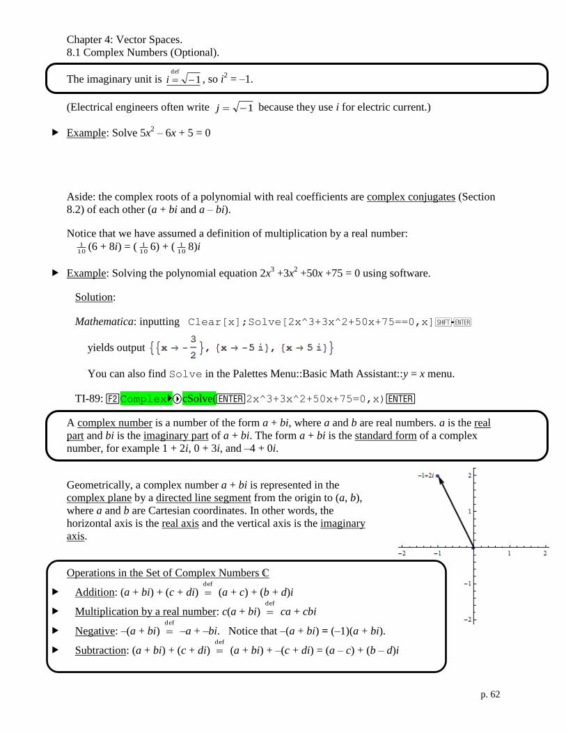
Chapter 4: Vector Spaces.
8.1 Complex Numbers (Optional).
p. 62
The imaginary unit is 1def
i , so i2 = –1.
(Electrical engineers often write 1j because they use i for electric current.)
Example: Solve 5x2 – 6x + 5 = 0
Aside: the complex roots of a polynomial with real coefficients are complex conjugates (Section
8.2) of each other (a + bi and a – bi).
Notice that we have assumed a definition of multiplication by a real number:
101 (6 + 8i) = (
101 6) + (
101 8)i
Example: Solving the polynomial equation 2x3 +3x
2 +50x +75 = 0 using software.
Solution:
Mathematica: inputting Clear[x];Solve[2x^3+3x^2+50x+75==0,x]
yields output
You can also find Solve in the Palettes Menu::Basic Math Assistant::y = x menu.
TI-89: ComplexcSolve(2x^3+3x^2+50x+75=0,x)
A complex number is a number of the form a + bi, where a and b are real numbers. a is the real
part and bi is the imaginary part of a + bi. The form a + bi is the standard form of a complex
number, for example 1 + 2i, 0 + 3i, and –4 + 0i.
Geometrically, a complex number a + bi is represented in the
complex plane by a directed line segment from the origin to (a, b),
where a and b are Cartesian coordinates. In other words, the
horizontal axis is the real axis and the vertical axis is the imaginary
axis.
Operations in the Set of Complex Numbers C
Addition: (a + bi) + (c + di) def
(a + c) + (b + d)i
Multiplication by a real number: c(a + bi) def
ca + cbi
Negative: –(a + bi) def
–a + –bi. Notice that –(a + bi) = (–1)(a + bi).
Subtraction: (a + bi) + (c + di) def
(a + bi) + –(c + di) = (a – c) + (b – d)i

Chapter 4: Vector Spaces.
8.1 Complex Numbers (Optional).
p. 63
Examples
Let z = 2 + 4i and w = –4 + 1i. Illustrate the following graphically.
z, w, z + w, 1.5z, – w, w – z

Chapter 4: Vector Spaces.
8.1 Complex Numbers (Optional).
p. 64
Multiplication of complex numbers is defined using the distributive property and using i 2
= –1.
(a + bi)(c + di) def
(ac – bd) + (ad + bc)i
because (a + bi)(c + di) = ac + adi + bci + bdi 2
= ac + adi + bci + bdi 2
= ac + adi + bci – bd
Warning: When you multiply square roots of negative numbers, convert into standard form
a + bi (not using the square root of a negative number) before you multiply. For example,
1 1 = i·i = –1, not 1 1 = )1)(1( = 1 = 1.
Application (Electrical Engineering): V(t)= I(t)Z, I(t)= current = I0 cos(t) + i I0 sin(t)
V(t) = volatge, Z = impedance = R + Ci
1 + Li ,
R = resistance, C = capacitance, L = inductance
Example: Use software to check that i5
4
5
3 is a zero of the polynomial 5x
2 – 6x + 5.
Solution:
Mathematica: to input the imaginary unit i, denoted by i in Mathematica, type ii (four
separate keystrokes). After the first three keystrokes, you will see ii. After the fourth
keystroke, ii will change to i.
Type x=3/5+4ii/55x^2-6x+5
TI-89: (3/5+4/5)
5x^2-6x+5
Complex matrices
Example: Find the inverse of A =
541
413
i
i by hand. Check your answer by multiplying.
Solution: A–1
=)det(
1
A
341
415
i
i.
det(A) = 5(3) – (–1 + 4i)(–1 – 4i) = 15 – (1 + 4i – 4i + 16) = –2
A–1
=2
1
341
415
i
i

Chapter 4: Vector Spaces.
8.1 Complex Numbers (Optional).
p. 65
Check: AA–1
=
541
413
i
i
2
1
341
415
i
i
=
2
1
1516441205205
1231231644115
iiii
iiii =
2
1
20
02 =
10
01
Example: By hand, find the determinant of
Example: Perform Gauss-Jordan elimination
using row operations to solve
iziyixiw
iziyxiiw
ziyxiw
3)716()62()36(3
31)53(3)42(2
22)2(


392 Chapter 8 Complex Vector Spaces
8.1 Complex Numbers
Use the imaginary unit to write complex numbers.
Graphically represent complex numbers in the complex plane aspoints and as vectors.
Add and subtract two complex numbers, and multiply a complexnumber by a real scalar.
Multiply two complex numbers, and use the Quadratic Formula tofind all zeros of a quadratic polynomial.
Perform operations with complex matrices, and find the determinantof a complex matrix.
COMPLEX NUMBERS
So far in the text, the scalar quantities used have been real numbers. In this chapter, youwill expand the set of scalars to include complex numbers.
In algebra it is often necessary to solve quadratic equations such asThe general quadratic equation is and its
solutions are given by the Quadratic Formula
where the quantity under the radical, is called the discriminant. Ifthen the solutions are ordinary real numbers. But what can you conclude
about the solutions of a quadratic equation whose discriminant is negative? Forinstance, the equation has a discriminant of but there isno real number whose square is To overcome this deficiency, mathematiciansinvented the imaginary unit defined as
where In terms of this imaginary unit,With this single addition of the imaginary unit to the real number system, the
system of complex numbers can be developed.
Some examples of complex numbers written in standard form are and The set of real numbers is a subset of the set of complex
numbers. To see this, note that every real number can be written as a complex number using That is, for every real number,
A complex number is uniquely determined by its real and imaginary parts. So, twocomplex numbers are equal if and only if their real and imaginary parts are equal. Thatis, if and are two complex numbers written in standard form, then
if and only if and b � d.a � c
a � bi � c � di
c � dia � bi
a � a � 0i.b � 0.a
�6i � 0 � 6i.4 � 3i,2 � 2 � 0i,
i��16 � 4��1 � 4i.i2 � �1.
i � ��1
i,�16.
b2 � 4ac � �16,x2 � 4 � 0
b2 � 4ac � 0,b2 � 4ac,
x ��b � �b2 � 4ac
2a
ax2 � bx � c � 0,x2 � 3x � 2 � 0.
i
REMARK
When working with productsinvolving square roots of negative numbers, be sure toconvert to a multiple of beforemultiplying. For instance, consider the following operations.
Correct
Incorrect � 1
� �1
��1��1 � ���1���1�
� �1
� i2
��1��1 � i � i
i
Definition of a Complex Number
If and are real numbers, then the number
is a complex number, where is the real part and is the imaginary part ofthe number. The form is the standard form of a complex number.a � bi
bia
a � bi
ba
9781133110873_0801.qxp 3/10/12 6:52 AM Page 392

THE COMPLEX PLANE
Because a complex number is uniquely determined by its real and imaginary parts,it is natural to associate the number with the ordered pair With this association, complex numbers can be represented graphically as points in a coordinateplane called the complex plane. This plane is an adaptation of the rectangular coordinate plane. Specifically, the horizontal axis is the real axis and the vertical axisis the imaginary axis. The point that corresponds to the complex number is
as shown in Figure 8.1.
Plotting Numbers in the Complex Plane
Plot each number in the complex plane.
a. b. c. d. 5
SOLUTION
Figure 8.2 shows the numbers plotted in the complex plane.
a. b.
c. d.
Figure 8.2
Another way to represent the complex number is as a vector whose horizontal component is and whose vertical component is (See Figure 8.3.) (Notethat the use of the letter to represent the imaginary unit is unrelated to the use of torepresent a unit vector.)
Vector Representation of a Complex Number
Figure 8.3
1
−1
−2
−3
4 − 2iVertical
component
Horizontalcomponent
Realaxis
Imaginaryaxis
iib.a
a � bi
5 or (5, 0)Realaxis
Imaginaryaxis
−1 1 2 3 4 5
−2
1
2
3
4
−3i or (0, −3)
Realaxis
Imaginaryaxis
−1−2−3 1 2 3
−3
−2
−4
1
2
−2 − i
Realaxis
Imaginaryaxis
−1−2−3 1 2 3
−3
−4
1
2
or (−2, −1)
4 + 3ior (4, 3)
Realaxis
Imaginaryaxis
−1−2 1 2 3 4
−2
1
2
3
4
�3i�2 � i4 � 3i
�a, b�,a � bi
�a, b�.a � bi
8.1 Complex Numbers 393
(a, b) or a + bi
Realaxis
Imaginaryaxis
The Complex Plane
a
b
Figure 8.1
9781133110873_0801.qxp 3/10/12 6:52 AM Page 393

394 Chapter 8 Complex Vector Spaces
ADDITION, SUBTRACTION, AND SCALAR
MULTIPLICATION OF COMPLEX NUMBERS
Because a complex number consists of a real part added to a multiple of the operations of addition and multiplication are defined in a manner consistent with therules for operating with real numbers. For instance, to add (or subtract) two complexnumbers, add (or subtract) the real and imaginary parts separately.
Adding and Subtracting Complex Numbers
a.
b.
Using the vector representation of complex numbers, you can add or subtract two complex numbers geometrically using the parallelogram rule for vector addition, asshown in Figure 8.4.
Figure 8.4
Many of the properties of addition of real numbers are valid for complex numbersas well. For instance, addition of complex numbers is both associative and commutative.Moreover, to find the sum of three or more complex numbers, extend the definition ofaddition in the natural way. For example,
� 3 � 3i.
�2 � i� � �3 � 2i� � ��2 � 4i� � �2 � 3 � 2� � �1 � 2 � 4�i
Realaxis
1
1
2
−3
−3 2 3
Imaginaryaxis
w = 3 + i
z = 1 − 3i
z − w = −2 − 4iSubtraction of Complex Numbers
1
−2
−3
−4
−1 2 3 41 65
2
3
4
Addition of Complex Numbersw = 2 − 4i
z + w = 5
z = 3 + 4i
Imaginaryaxis
Realaxis
� �2 � 4i
�1 � 3i� � �3 � i� � �1 � 3� � ��3 � 1�i � 5
�2 � 4i� � �3 � 4i� � �2 � 3� � ��4 � 4�i
i,
Definition of Addition and Subtraction of Complex Numbers
The sum and difference of
and
are defined as follows.
Sum
Difference�a � bi� � �c � di� � �a � c� � �b � d �i
�a � bi� � �c � di� � �a � c� � �b � d �i
c � dia � bi
REMARK
Note in part (a) of Example 2that the sum of two complexnumbers can be a real number.
9781133110873_0801.qxp 3/10/12 6:52 AM Page 394
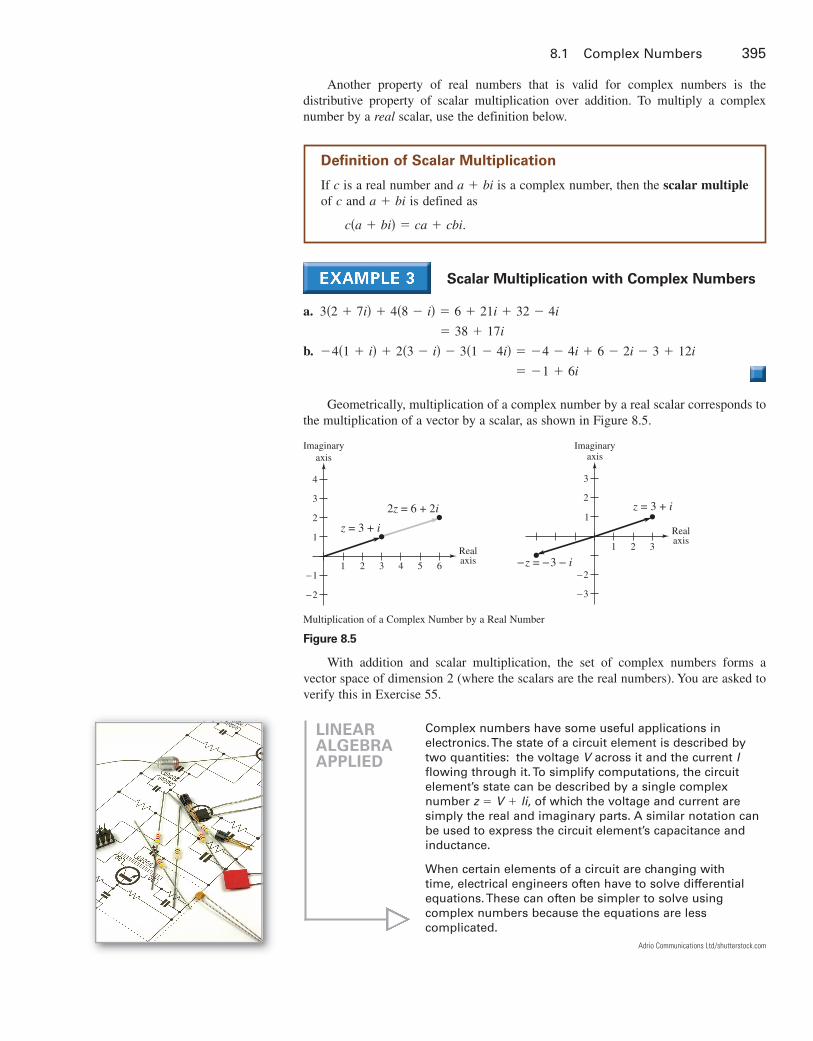
Another property of real numbers that is valid for complex numbers is the distributive property of scalar multiplication over addition. To multiply a complex number by a real scalar, use the definition below.
Scalar Multiplication with Complex Numbers
a.
b.
Geometrically, multiplication of a complex number by a real scalar corresponds tothe multiplication of a vector by a scalar, as shown in Figure 8.5.
Multiplication of a Complex Number by a Real Number
Figure 8.5
With addition and scalar multiplication, the set of complex numbers forms a vector space of dimension 2 (where the scalars are the real numbers). You are asked toverify this in Exercise 55.
Imaginaryaxis
Realaxis
1
1
2
−2
−3
3
2 3
−z = −3 − i
z = 3 + i
Realaxis
z = 3 + i
2z = 6 + 2i
1
1
2
−1
−2
3
4
2 3 4 65
Imaginaryaxis
� �1 � 6i
�4�1 � i� � 2�3 � i� � 3�1 � 4i� � �4 � 4i � 6 � 2i � 3 � 12i
� 38 � 17i
3�2 � 7i� � 4�8 � i� � 6 � 21i � 32 � 4i
8.1 Complex Numbers 395
LINEAR ALGEBRA APPLIED
Complex numbers have some useful applications in electronics. The state of a circuit element is described bytwo quantities: the voltage across it and the current flowing through it. To simplify computations, the circuit element’s state can be described by a single complex number of which the voltage and current aresimply the real and imaginary parts. A similar notation canbe used to express the circuit element’s capacitance andinductance.
When certain elements of a circuit are changing with time, electrical engineers often have to solve differentialequations. These can often be simpler to solve using complex numbers because the equations are less complicated.
z � V � li,
IV
Definition of Scalar Multiplication
If is a real number and is a complex number, then the scalar multipleof and is defined as
c�a � bi� � ca � cbi.
a � bica � bic
Adrio Communications Ltd/shutterstock.com
9781133110873_0801.qxp 3/10/12 6:52 AM Page 395
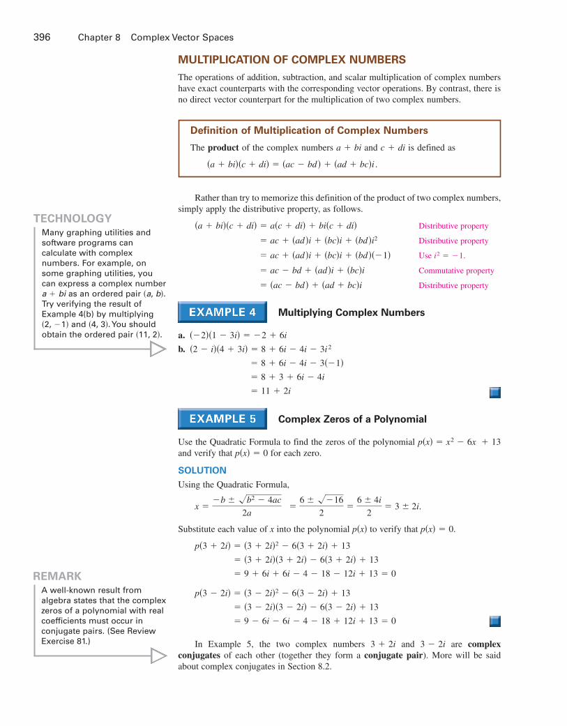
396 Chapter 8 Complex Vector Spaces
MULTIPLICATION OF COMPLEX NUMBERS
The operations of addition, subtraction, and scalar multiplication of complex numbershave exact counterparts with the corresponding vector operations. By contrast, there isno direct vector counterpart for the multiplication of two complex numbers.
Rather than try to memorize this definition of the product of two complex numbers,simply apply the distributive property, as follows.
Distributive property
Distributive property
Use
Commutative property
Distributive property
Multiplying Complex Numbers
a.
b.
Complex Zeros of a Polynomial
Use the Quadratic Formula to find the zeros of the polynomial and verify that for each zero.
SOLUTION
Using the Quadratic Formula,
Substitute each value of into the polynomial to verify that
In Example 5, the two complex numbers and are complex conjugates of each other (together they form a conjugate pair). More will be saidabout complex conjugates in Section 8.2.
3 � 2i3 � 2i
� 0 � 9 � 6i � 6i � 4 � 18 � 12i � 13
� �3 � 2i��3 � 2i� � 6�3 � 2i� � 13
p�3 � 2i� � �3 � 2i�2 � 6�3 � 2i� � 13
� 0 � 9 � 6i � 6i � 4 � 18 � 12i � 13
� �3 � 2i��3 � 2i� � 6�3 � 2i� � 13
p�3 � 2i� � �3 � 2i�2 � 6�3 � 2i� � 13
p�x� � 0.p�x�x
�6 � ��16
2�
6 � 4i
2� 3 � 2i. x �
�b � �b2 � 4ac
2a
p�x� � 0p�x� � x2 � 6x � 13
� 11 � 2i
� 8 � 3 � 6i � 4i
� 8 � 6i � 4i � 3��1� �2 � i��4 � 3i� � 8 � 6i � 4i � 3i2
��2��1 � 3i� � �2 � 6i
� �ac � bd � � �ad � bc�i � ac � bd � �ad �i � �bc�i
i2 � �1. � ac � �ad �i � �bc�i � �bd ���1� � ac � �ad �i � �bc�i � �bd �i2
�a � bi��c � di� � a�c � di� � bi�c � di�TECHNOLOGY
Many graphing utilities andsoftware programs can calculate with complex numbers. For example, onsome graphing utilities, youcan express a complex number
as an ordered pair Try verifying the result ofExample 4(b) by multiplying
and You shouldobtain the ordered pair �11, 2�.
�4, 3�.�2, �1�
�a, b�.a � bi
Definition of Multiplication of Complex Numbers
The product of the complex numbers and is defined as
�a � bi��c � di� � �ac � bd � � �ad � bc�i .
c � dia � bi
REMARK
A well-known result from algebra states that the complexzeros of a polynomial with realcoefficients must occur in conjugate pairs. (See ReviewExercise 81.)
9781133110873_0801.qxp 3/10/12 6:52 AM Page 396

COMPLEX MATRICES
Now that you are able to add, subtract, and multiply complex numbers, you can applythese operations to matrices whose entries are complex numbers. Such a matrix iscalled complex.
All of the ordinary operations with matrices also work with complex matrices, asdemonstrated in the next two examples.
Operations with Complex Matrices
Let and be the complex matrices
and
and determine each of the following.
a. b. c. d.
SOLUTION
a.
b.
c.
d.
Finding the Determinant of a Complex Matrix
Find the determinant of the matrix
SOLUTION
� �8 � 26i
� 10 � 20i � 6i � 12 � 6
� �2 � 4i��5 � 3i� � �2��3�
det�A� � �2 � 4i3
25 � 3i�
A � �2 � 4i3
25 � 3i�.
� � �27 � i
�2 � 2i3 � 9i�
� � �2 � 0�1 � 2 � 3i � 4i � 6
2i � 2 � 0i � 1 � 4 � 8i�
BA � �2ii
01 � 2i��
i2 � 3i
1 � i4�
A � B � � i2 � 3i
1 � i4� � �2i
i0
1 � 2i� � � 3i2 � 2i
1 � i5 � 2i�
�2 � i�B � �2 � i��2ii
01 � 2i� � �2 � 4i
1 � 2i0
4 � 3i�
3A � 3� i2 � 3i
1 � i4� � � 3i
6 � 9i3 � 3i
12�
BAA � B�2 � i�B3A
B � �2ii
01 � 2i�A � � i
2 � 3i1 � i
4�BA
8.1 Complex Numbers 397
Definition of a Complex Matrix
A matrix whose entries are complex numbers is called a complex matrix.
TECHNOLOGY
Many graphing utilities andsoftware programs can performmatrix operations on complexmatrices. Try verifying the calculation of the determinantof the matrix in Example 7. You should obtain the sameanswer, ��8, �26�.
9781133110873_0801.qxp 3/10/12 6:52 AM Page 397

398 Chapter 8 Complex Vector Spaces
8.1 Exercises
Simplifying an Expression In Exercises 1–6, determinethe value of the expression.
1. 2. 3.
4. 5. 6.
Equality of Complex Numbers In Exercises 7–10,determine such that the complex numbers in each pairare equal.
7.
8.
9.
10.
Plotting Complex Numbers In Exercises 11–16, plotthe number in the complex plane.
11. 12. 13.
14. 15. 16.
Adding and Subtracting Complex Numbers InExercises 17–24, find the sum or difference of the complex numbers. Use vectors to illustrate your answer.
17. 18.
19. 20.
21. 22.
23. 24.
Scalar Multiplication In Exercises 25 and 26, use vectors to illustrate the operations geometrically. Be sureto graph the original vector.
25. and , where
26. and , where
Multiplying Complex Numbers In Exercises 27–34,find the product.
27. 28.
29. 30.
31. 32.
33. 34.
Finding Zeros In Exercises 35–40, determine all thezeros of the polynomial function.
35. 36.
37. 38.
39. 40.
Finding Zeros In Exercises 41–44, use the given zeroto find all zeros of the polynomial function.
41. Zero:
42. Zero:
43. Zero:
44. Zero:
Operations with Complex Matrices In Exercises45–54, perform the indicated matrix operation using thecomplex matrices and
and
45. 46.
47. 48.
49. 50.
51. det 52. det
53. 54.
55. Proof Prove that the set of complex numbers, with theoperations of addition and scalar multiplication (withreal scalars), is a vector space of dimension 2.
57. (a) Evaluate for and 5.
(b) Calculate
(c) Find a general formula for for any positive integer
58. Let
(a) Calculate for and 5.
(b) Calculate
(c) Find a general formula for for any positive integer
True or False? In Exercises 59 and 60, determinewhether each statement is true or false. If a statement istrue, give a reason or cite an appropriate statement fromthe text. If a statement is false, provide an example thatshows the statement is not true in all cases or cite anappropriate statement from the text.
59. 60.
61. Proof Prove that if the product of two complex numbersis zero, then at least one of the numbers must be zero.
���10�2 � �100 � 10��2��2 � �4 � 2
n.An
A2010.
n � 1, 2, 3, 4,An
A � �0i
i0�.
n.in
i2010.
n � 1, 2, 3, 4,in
BA5AB
�B��A � B�
14iB2iA
12B2A
B � AA � B
B � �1 � i�3
3i�i�A � � 1 � i
2 � 2i1
�3i�B.A
x � 3ip�x� � x3 � x2 � 9x � 9
x � 5ip�x� � 2x3 � 3x2 � 50x � 75
x � �4p�x� � x3 � 2x2 � 11x � 52
x � 1p�x� � x3 � 3x2 � 4x � 2
p�x� � x4 � 10x2 � 9p�x� � x4 � 16
p�x� � x2 � 4x � 5p�x� � x2 � 5x � 6
p�x� � x2 � x � 1p�x� � 2x2 � 2x � 5
�2 � i��2 � 2i��4 � i��1 � i�3
�a � bi��a � bi��a � bi�2
�4 � �2 i��4 � �2 i ���7 � i���7 � i��3 � i�� 2
3 � i��5 � 5i��1 � 3i�
u � 2 � i�32u3u
u � 3 � i2u�u
�2 � i� � �2 � i��2 � i� � �2 � i��12 � 7i� � �3 � 4i�6 � ��2i�i � �3 � i��5 � i� � �5 � i��1 � �2 i� � �2 � �2 i��2 � 6i� � �3 � 3i�
z � 1 � 5iz � 1 � 5iz � 7
z � �5 � 5iz � 3iz � 6 � 2i
��x � 4� � �x � 1�i, x � 3i
�x2 � 6� � �2x�i, 15 � 6i
�2x � 8� � �x � 1�i, 2 � 4i
x � 3i, 6 � 3i
x
��i�7i 4i 3
��4��4�8��8��2��3
56. Consider the functions and
(a) Without graphing either function, determinewhether the graphs of and have -intercepts.Explain your reasoning.
(b) For which of the given functions is azero? Without using the Quadratic Formula, find theother zero of this function and verify your answer.
x � 3 � i
xqp
q�x� � x2 � 6x � 10.p�x� � x2 � 6x � 10
9781133110873_0801.qxp 3/10/12 6:52 AM Page 398
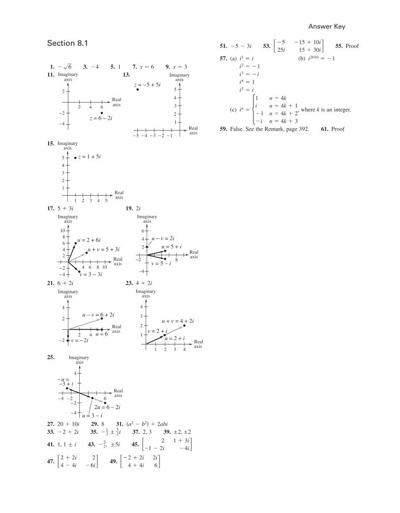
Section 8.1
1. 3. 5. 1 7. 9.11. 13.
15.
17. 19.
21. 23.
25.
27. 29. 8 31.33. 35. 37. 2, 3 39.
41. 43. 45.
47. 49.
51. 53. 55. Proof
57. (a) (b)
(c) , where is an integer.
59. False. See the Remark, page 392. 61. Proof
kin � �1i�1�i
n � 4kn � 4k � 1n � 4k � 2n � 4k � 3
i5 � ii4 � 1i3 � �ii2 � �1
i2010 � �1i1 � i
��525i
�15 � 10i15 � 30i��5 � 3i
��2 � 2i4 � 4i
2i6��2 � 2i
4 � 4i 2
�6i�� 2�1 � 2i
1 � 3i�4i��
32, ±5i1, 1 ± i
±2, ±2�12 ± 3
2i�2 � 2i�a2 � b2� � 2abi20 � 10i
4
Imaginary axis
−u = −3 + i
u = 3 − i
2u = 6 − 2i−2
−2
−4
−4 6
Realaxis
1
2
3
4
1 2 3 4
Realaxis
Imaginaryaxis
u = 2 + iv = 2 + i
u + v = 4 + 2i
4
2
−22 4
Realaxisu = 6
v = −2i
u − v = 6 + 2i
Imaginaryaxis
4 � 2i6 � 2i
Realaxis
Imaginaryaxis
−2
−4
2
4
6
8v = 5 − i
u − v = 2i
u = 5 + i
24
4
68
10
Imaginaryaxis
−2−4
6 8 10
u = 2 + 6i
v = 3 − 3i
u + v = 5 + 3i
Realaxis
2i5 � 3i
Realaxis
axis
1
2
3
4
5
1 2 3 4 5
z = 1 + 5i
Imaginary
Realaxis
axis
1
2
3
4
5
−1−2−3−4−5
z = −5 + 5i
Imaginary
2
−2
−4
axis
Realaxis
z = 6 − 2i
2 4 6
Imaginary
x � 3x � 6�4��6
Answer Key
9781133110873_08_ANS.qxd 3/10/12 6:58 AM Page A1
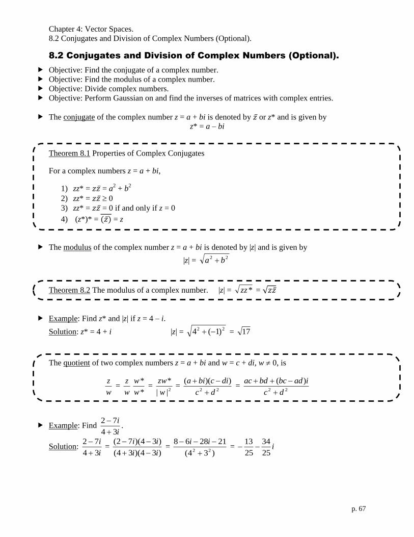
Chapter 4: Vector Spaces.
8.2 Conjugates and Division of Complex Numbers (Optional).
p. 67
8.2 Conjugates and Division of Complex Numbers (Optional).
Objective: Find the conjugate of a complex number.
Objective: Find the modulus of a complex number.
Objective: Divide complex numbers.
Objective: Perform Gaussian on and find the inverses of matrices with complex entries.
The conjugate of the complex number z = a + bi is denoted by 𝑧̅ or z* and is given by
z* = a – bi
Theorem 8.1 Properties of Complex Conjugates
For a complex numbers z = a + bi,
1) zz* = 𝑧𝑧̅ = a2 + b
2
2) zz* = 𝑧𝑧̅ 0
3) zz* = 𝑧𝑧̅ = 0 if and only if z = 0
4) (z*)* = (𝑧̅) = z
The modulus of the complex number z = a + bi is denoted by |z| and is given by
|z| = 22 ba
Theorem 8.2 The modulus of a complex number. |z| = *zz = √𝑧𝑧̅
Example: Find z* and |z| if z = 4 – i.
Solution: z* = 4 + i |z| = 22 )1(4 = 17
The quotient of two complex numbers z = a + bi and w = c + di, w 0, is
w
z =
w
z
*
*
w
w =
2||
*
w
zw =
22
))((
dc
dicbia
=
22
)(
dc
iadbcbdac
Example: Findi
i
34
72
.
Solution: i
i
34
72
=
)34)(34(
)34)(72(
ii
ii
=
)34(
21286822
ii = i
25
34
25
13
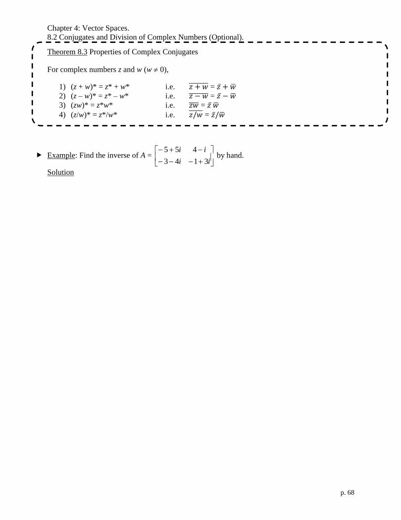
Chapter 4: Vector Spaces.
8.2 Conjugates and Division of Complex Numbers (Optional).
p. 68
Theorem 8.3 Properties of Complex Conjugates
For complex numbers z and w (w 0),
1) (z + w)* = z* + w* i.e. 𝑧 + 𝑤̅̅ ̅̅ ̅̅ ̅̅ = 𝑧̅ + �̅�
2) (z – w)* = z* – w* i.e. 𝑧 − 𝑤̅̅ ̅̅ ̅̅ ̅̅ = 𝑧̅ − �̅�
3) (zw)* = z*w* i.e. 𝑧𝑤̅̅ ̅̅ = 𝑧̅ �̅�
4) (z/w)* = z*/w* i.e. 𝑧/𝑤̅̅ ̅̅ ̅ = 𝑧̅/�̅�
Example: Find the inverse of A =
ii
ii
3143
455 by hand.
Solution

Chapter 4: Vector Spaces.
8.2 Conjugates and Division of Complex Numbers (Optional).
p. 69
Example: Perform Gaussian elimination using row operations to solve
iziiyxi
iziiyix
iziyixi
10057)1615(20)55(
5767)1012(72
452)39()48()3(
Solution:

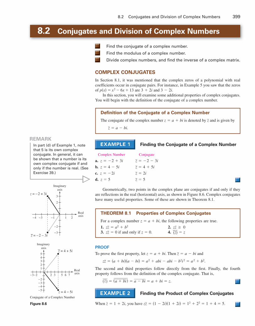
8.2 Conjugates and Division of Complex Numbers 399
8.2 Conjugates and Division of Complex Numbers
Find the conjugate of a complex number.
Find the modulus of a complex number.
Divide complex numbers, and find the inverse of a complex matrix.
COMPLEX CONJUGATES
In Section 8.1, it was mentioned that the complex zeros of a polynomial with real coefficients occur in conjugate pairs. For instance, in Example 5 you saw that the zerosof are and
In this section, you will examine some additional properties of complex conjugates.You will begin with the definition of the conjugate of a complex number.
Finding the Conjugate of a Complex Number
Complex Number Conjugate
a.
b.
c.
d.
Geometrically, two points in the complex plane are conjugates if and only if theyare reflections in the real (horizontal) axis, as shown in Figure 8.6. Complex conjugateshave many useful properties. Some of these are shown in Theorem 8.1.
PROOF
To prove the first property, let Then and
The second and third properties follow directly from the first. Finally, the fourth property follows from the definition of the complex conjugate. That is,
Finding the Product of Complex Conjugates
When you have zz � �1 � 2i��1 � 2i� � 12 � 22 � 1 � 4 � 5.z � 1 � 2i,
� a � bi � a � bi � z.� �a � bi��z�
zz � �a � bi��a � bi� � a2 � abi � abi � b2i2 � a2 � b2.
z � a � biz � a � bi.
z � 5z � 5
z � 2iz � �2i
z � 4 � 5iz � 4 � 5i
z � �2 � 3iz � �2 � 3i
3 � 2i.3 � 2ip�x� � x2 � 6x � 13
Definition of the Conjugate of a Complex Number
The conjugate of the complex number is denoted by and is given by
z � a � bi.
zz � a � bi
REMARK
In part (d) of Example 1, notethat 5 is its own complex conjugate. In general, it can be shown that a number is itsown complex conjugate if andonly if the number is real. (SeeExercise 39.)
Conjugate of a Complex Number
Figure 8.6
Realaxis2 3−2
−2−3−4−5
−3 5 6 7
12345
z = 4 − 5i
z = 4 + 5i
Imaginary axis
Realaxis
z = −2 − 3i
z = −2 + 3i
2
−2
−3
−3−4 −1 1 2
3
Imaginaryaxis
THEOREM 8.1 Properties of Complex Conjugates
For a complex number the following properties are true.
1. 2.3. if and only if 4. �z� � zz � 0.zz � 0
zz � 0zz � a2 � b2
z � a � bi,
9781133110873_0802.qxp 3/14/12 8:23 AM Page 399

400 Chapter 8 Complex Vector Spaces
THE MODULUS OF A COMPLEX NUMBER
Because a complex number can be represented by a vector in the complex plane, itmakes sense to talk about the length of a complex number. This length is called themodulus of the complex number.
Finding the Modulus of a Complex Number
For and determine the value of each modulus.
a. b. c.
SOLUTION
a.
b.
c. Because you have
Note that in Example 3, In Exercise 41, you are asked to prove that this multiplicative property of the modulus always holds. Theorem 8.2 states that themodulus of a complex number is related to its conjugate.
PROOF
Let then and zz � �a � bi��a � bi� � a2 � b2 � �z�2.z � a � biz � a � bi,
�zw� � �z� �w�.
�zw� � �152 � 162 � �481.
zw � �2 � 3i��6 � i� � 15 � 16i,�w� � �62 � ��1�2 � �37�z� � �22 � 32 � �13
�zw��w��z�w � 6 � i,z � 2 � 3i
Definition of the Modulus of a Complex Number
The modulus of the complex number is denoted by and is given by
�z� � �a2 � b2.
�z�z � a � bi
LINEAR ALGEBRA APPLIED
Fractals appear in almost every part of the universe. Theyhave been used to study a wide variety of applications suchas bacteria cultures, the human lungs, the economy, andgalaxies. The most famous fractal is called the MandelbrotSet, named after the Polish-born mathematician BenoitMandelbrot (1924–2010). The Mandelbrot Set is based onthe following sequence of complex numbers.
The behavior of this sequence depends on the value of thecomplex number For some values of the modulus ofeach term in the sequence is less than some fixed number
and the sequence is bounded. This means that is in theMandelbrot Set, and its point is colored black. For other values of the moduli of the terms of the sequence becomeinfinitely large, and the sequence is unbounded. This meansthat is not in the Mandelbrot Set, and its point is assigned a color based on “how quickly” the sequence diverges.
c
c,
cN,zn
c,c.
zn � �zn�1�2 � c, z1 � c
REMARK
The modulus of a complexnumber is also called theabsolute value of the number.In fact, when is a real number,
�z� � �a2 � 02 � �a�.z
THEOREM 8.2 The Modulus of a Complex Number
For a complex number �z�2 � zz.z,
Andrew Park/Shutterstock.com
9781133110873_0802.qxp 3/10/12 6:57 AM Page 400
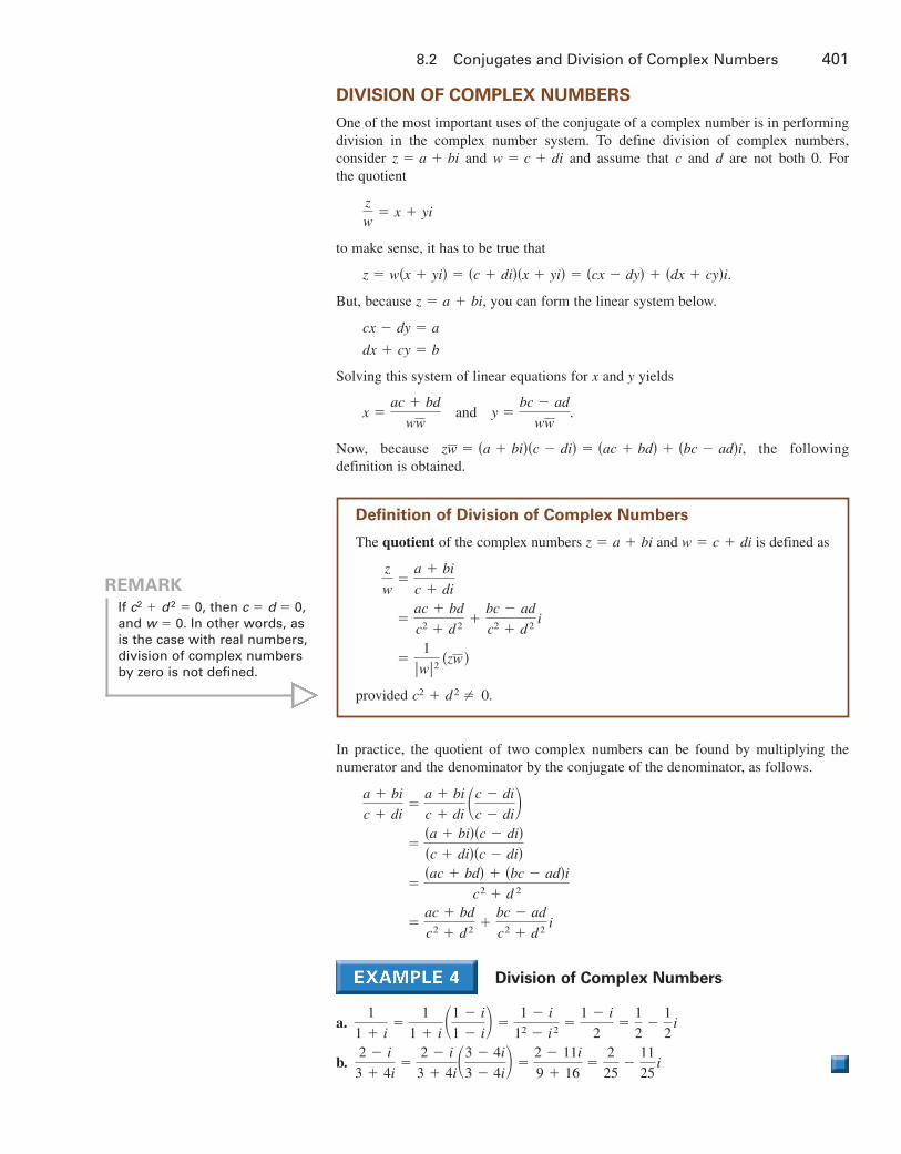
8.2 Conjugates and Division of Complex Numbers 401
DIVISION OF COMPLEX NUMBERS
One of the most important uses of the conjugate of a complex number is in performingdivision in the complex number system. To define division of complex numbers,consider and and assume that and are not both 0. For the quotient
to make sense, it has to be true that
But, because you can form the linear system below.
Solving this system of linear equations for and yields
and
Now, because the following definition is obtained.
In practice, the quotient of two complex numbers can be found by multiplying thenumerator and the denominator by the conjugate of the denominator, as follows.
Division of Complex Numbers
a.
b.2 � i
3 � 4i�
2 � i
3 � 4i�3 � 4i
3 � 4i� �2 � 11i
9 � 16�
2
25�
11
25i
1
1 � i�
1
1 � i �1 � i
1 � i� �1 � i
12 � i2�
1 � i
2�
1
2�
1
2i
�ac � bd
c2 � d2�
bc � ad
c2 � d2i
��ac � bd� � �bc � ad�i
c2 � d 2
��a � bi��c � di��c � di��c � di�
a � bi
c � di�
a � bi
c � di �c � di
c � di�
zw � �a � bi��c � di� � �ac � bd� � �bc � ad�i,
y �bc � ad
ww.x �
ac � bd
ww
yx
dx � cy � b
cx � dy � a
z � a � bi,
z � w�x � yi� � �c � di��x � yi� � �cx � dy� � �dx � cy�i.
zw
� x � yi
dcw � c � diz � a � bi
Definition of Division of Complex Numbers
The quotient of the complex numbers and is defined as
provided c2 � d2 � 0.
�1
�w�2 �zw �
�ac � bd
c2 � d2�
bc � ad
c2 � d2i
z
w�
a � bi
c � di
w � c � diz � a � bi
REMARK
If then and In other words, asis the case with real numbers,division of complex numbersby zero is not defined.
w � 0.c � d � 0,c2 � d2 � 0,
9781133110873_0802.qxp 3/10/12 6:57 AM Page 401
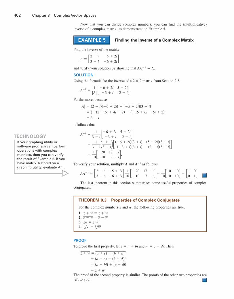
402 Chapter 8 Complex Vector Spaces
Now that you can divide complex numbers, you can find the (multiplicative)inverse of a complex matrix, as demonstrated in Example 5.
Finding the Inverse of a Complex Matrix
Find the inverse of the matrix
and verify your solution by showing that
SOLUTION
Using the formula for the inverse of a matrix from Section 2.3,
Furthermore, because
it follows that
To verify your solution, multiply and as follows.
The last theorem in this section summarizes some useful properties of complexconjugates.
PROOF
To prove the first property, let and Then
The proof of the second property is similar. The proofs of the other two properties areleft to you.
� z � w.
� �a � bi� � �c � di� � �a � c� � �b � d �i
z � w � �a � c� � �b � d�i
w � c � di.z � a � bi
� �10
01�
110�
100
010 AA�1 � �2 � i
3 � i�5 � 2i�6 � 2i
110
��20�10
17 � i7 � i
A�1A
�110�
�20�10
17 � i7 � i.
�1
3 � i�1
3 � i����6 � 2i��3 � i���3 � i��3 � i�
�5 � 2i��3 � i��2 � i��3 � i�
A�1 �1
3 � i ��6 � 2i�3 � i
5 � 2i2 � i
� 3 � i
� ��12 � 6i � 4i � 2� � ��15 � 6i � 5i � 2� �A� � �2 � i���6 � 2i� � ��5 � 2i��3 � i�
A�1 �1
�A� ��6 � 2i�3 � i
5 � 2i2 � i.
2 � 2
AA�1 � I2.
A � �2 � i
3 � i
�5 � 2i
�6 � 2i
TECHNOLOGY
If your graphing utility or software program can performoperations with complex matrices, then you can verifythe result of Example 5. If youhave matrix stored on agraphing utility, evaluate A�1.
A
THEOREM 8.3 Properties of Complex Conjugates
For the complex numbers and the following properties are true.
1.2.3.4. zw � zw
zw � z wz � w � z � wz � w � z � w
w,z
9781133110873_0802.qxp 3/10/12 6:57 AM Page 402

8.2 Exercises 403
8.2 Exercises
40. Consider the quotient
(a) Without performing any calculations, describehow to find the quotient.
(b) Explain why the process described in part (a)results in a complex number of the form
(c) Find the quotient.
a � bi.
1 � i6 � 2i
.
Finding the Conjugate In Exercises 1–6, find the complex conjugate and geometrically represent both
and
1. 2.
3. 4.
5. 6.
Finding the Modulus In Exercises 7–12, find the indicated modulus, where and
7. 8.
9. 10.
11. 12.
13. Verify that where and
14. Verify that where and
Dividing Complex Numbers In Exercises 15–20,perform the indicated operations.
15. 16.
17. 18.
19. 20.
Operations with Complex Rational Expressions InExercises 21–24, perform the operation and write theresult in standard form.
21. 22.
23. 24.
Finding Zeros In Exercises 25–28, use the given zero tofind all zeros of the polynomial function.
25. Zero:
26. Zero:
27. Zero:
28. Zero:
Powers of Complex Numbers In Exercises 29 and 30,find each power of the complex number
(a) (b) (c) (d)
29. 30.
Finding the Inverse of a Complex Matrix In Exercises31–36, determine whether the complex matrix has aninverse. If is invertible, find its inverse and verify that
31. 32.
33. 34.
35. 36.
Singular Matrices In Exercises 37 and 38, determineall values of the complex number for which is singular. (Hint: Set and solve for )
37. 38.
39. Proof Prove that if and only if is real.
41. Proof Prove that for any two complex numbers andeach of the statements below is true.
(a)
(b) If then
42. Graphical Interpretation Describe the set ofpoints in the complex plane that satisfies each of thestatements below.
(a) (b)
(c) (d)
43. (a) Evaluate for 1, 2, 3, 4, and 5.
(b) Calculate and
(c) Find a general formula for for any positiveinteger
44. (a) Verify that
(b) Find the two square roots of
(c) Find all zeros of the polynomial x4 � 1.
i.
�1 � i�2 �2
� i.
n.�1i�n
�1i�2010.�1i�2000
n ��1i�n
2 � �z� � 5�z � i� � 2�z � 1 � i� � 5�z� � 3
�zw� � �z��w�.w � 0,�zw� � �z��w�
w,z
zz � z
A � �2
1 � i1
2i1 � i
0
1 � iz0A � � 5
3iz
2 � i
z.det�A� � 0Az
A � �100
01 � i
0
00
1 � iA � �i00
0i0
00i
A � �1 � i0
21 � iA � �1 � i
12
1 � i
A � �2i3
�2 � i3iA � � 6
2 � i3ii
AA�1 � I.A
A
z � 1 � iz � 2 � i
z�2z�1z3z2
z.
�1 � 3ip�x� � x3 � 4x2 � 14x � 20
�3 � �2 ip�x� � x4 � 3x3 � 5x2 � 21x � 22
�3 � ip�x� � 4x3 � 23x2 � 34x � 10
1 � �3 ip�x� � 3x3 � 4x2 � 8x � 8
1 � i
i�
3
4 � i
i
3 � i�
2i
3 � i
2i
2 � i�
5
2 � i
2
1 � i�
3
1 � i
3 � i
�2 � i��5 � 2i��2 � i��3 � i�
4 � 2i
5 � i
4 � i
3 � �2 i
3 � �2 i
1
6 � 3i
2 � i
i
v � �2 � 3i.z � 1 � 2i�zv2� � �z��v2� � �z��v�2,
w � �1 � 2i.z � 1 � i�wz� � �w��z� � �zw�,
�zv2��v��wz��zw��z2��z�
v � �5i.w � �3 � 2i,z � 2 � i,
z � �3z � 4
z � 2iz � �8i
z � 2 � 5iz � 6 � 3i
z.zz
9781133110873_0802.qxp 3/10/12 6:57 AM Page 403

Section 8.2 1. 3.
5. 4
7. 9. 11. 513.
15. 19.
21. 23. 25.
27.29. (a) (b) (c) (d)
31. 33. Not invertible
35. 37.
39. Proof 41. (a) and (b) Proofs43. (a)
(b)
where k is an integer(c) �1�i�n � �1
�i�1
i
n � 4k n � 4k � 1n � 4k � 2n � 4k � 3
,
�1�i�1 � 1�i � �i, �1�i�2 � �1, �1�i�3 � i,�1�i�4 � 1, �1�i�5 � �i�1�i�2000 � 1, �1�i�2010 � �1
53� �
103 iA�1 � �
�i00
0�i
0
00
� i�
A�1 � �13� i
�2 � i�3i
6�325 �
425i2
5 �15i2 � 11i3 � 4i
1, 2, �3 ± �2 i
23� , 1 ± �3i1
10 �910i�
12
52� i
13
10�
9
10i
71 � 2i 17.
11�
6�2
11 i
wz � �3 � i � �10
wz � �5�2 � �10
zw � �3 � i � �10
�65�5
1
2
3
−1
−2
31 2 4 5
z and z = 4Realaxis
Imaginaryaxis
4
8
84−4
−4
−8
−8
z = 8i
z = −8i
Imaginaryaxis
642
2
4
z = 6 − 3i
z = 6 + 3i
Realaxis
Imaginaryaxis
−2
−4
8i6 � 3i
Answer Key

Chapter 4: Vector Spaces.
4.1 Vectors in Rn.
p. 71
4.1 Vectors in Rn.
Objective: Represent a vector in the plane as a directed line segment.
Objective: Perform basic vector operations in R2 and represent them graphically.
Objective: Perform basic vector operations in Rn.
Prove basic properties about vectors and their operations in Rn.
In physics and engineering, a vector is an object with magnitude and direction and represented
graphically by a directed line segment. In mathematics we have a much more general definition
of a vector.
Geometrically, a vector in the plane is represented by a directed line segment with its initial point
at the origin and its terminal (final) point at (x1, x2). The same ordered pair used to represent the
terminal point is used to represent the vector. That is, x = (x1, x2). The coordinates x1 and x2 are
called the components of the vector x. Two vectors u = (u1, u2) and v = (v1, v2) are equal iff u1 =
v1 and u2 = v2.
Vector operations in R2
Vector Addition: u + v = (u1, u2) + (v1, v2)def
(u1 + v1, u2 + v2).
Scalar Multiplication: cu = c(u1, u2)def
(cu1, cu2).
Negative: –udef
(–u1, –u2). Notice that –u = (–1)u.
Subtraction: u – vdef
u + (–v) = (u1, u2) + (–v1, –v2) = (u1 – v1, u2 – v2).
The zero vector in R2 is 0 = (0, 0).

Chapter 4: Vector Spaces.
4.1 Vectors in Rn.
p. 72
Examples
Let u = (2, 4) and v = (–4, 1). Illustrate the following graphically.
u, v, u + v, 1.5u, – v, v – u

Chapter 4: Vector Spaces.
4.1 Vectors in Rn.
p. 73
Theorem 4.1 Properties of Vector Addition and Scalar Multiplication in the Plane (R2)
Let u, v, and w be vectors in R2, and let c and d be scalars.
1) u + v is a vector in R2. Closure under addition
2) u + v = v + u Commutative property of addition
3) (u + v) + w = u + (v + w) Associative property of addition
4) u + 0 = u Existence of additive identity
5) u + (–u) = 0 Existence of additive inverses
6) cv is a vector in R2. Closure under scalar multiplication
7) c(u + v) = cu + cv Distributive property over vector addition
8) (c + d)u = cu + du Distributive property over scalar addition
9) c(du) = (cd)u Associative property
10) 1u = u Multiplicative identity property
Proof of (3): Associative property of addition
(u + v) + w = [(u1, u2) + (v1, v2)] + (w1, w2)
=
=
= Assoc. prop. of addition of real numbers
=
=
= u + (v + w)

Chapter 4: Vector Spaces.
4.1 Vectors in Rn.
p. 74
Proof of (8): Distributive property of scalar multiplication over real number addition
(c + d)u = (c + d)(u1, u2)
=
= Distributive property of real numbers
=
=
= cu + du
To add (1, 4) + (2, –2) in Mathematica, type {1,4}+{2,-2}
You can also assign a variable by typing u={1,4}
You can perform scalar multiplication by 3u or 3*u
To add (1, 4) + (2, –2) on the TI-89, you can type 1,4
+
2,-2
or 1
4
+
2
-2
You can also assign a variable by typing 1,4
U
You can perform scalar multiplication by 3u or 3u
Vector operations in Rn
We can generalize from the 2-dimensional plane R2 to an n-space Rn
of ordered n-tuples. For
example, R1 = R = set of all real numbers; R2
= 2-space = set of all ordered pairs of real
numbers; R3 = 3-space = set of all ordered triples of real numbers.\
An n-tuple (x1, x2, …, xn) can be viewed as a point in Rn with the xi as its coordinates, or as a
vector with the xi as its components.
The standard vector operations in Rn are
Vector Addition: u + v = (u1, u2, …, un) + (v1, v2, …, vn) def
(u1 + v1, u2 + v2, …, un + vn).
Scalar Multiplication: cu = c(u1, u2, …, un) def
(cu1, cu2, …, cun).
Negative: –u def
(–u1, –u2, …, –un). Notice that –u = (–1)u.
Subtraction: u – v def
u + (–v) = (u1, u2, …, un) + (–v1, –v2, …, –vn)
= (u1 – v1, u2 – v2, …, un – vn).
The zero vector in Rn is 0 = (0, 0, …, 0).

Chapter 4: Vector Spaces.
4.1 Vectors in Rn.
p. 75
Theorem 4.2 Properties of Vector Addition and Scalar Multiplication in the Plane (Rn)
Let u, v, and w be vectors in Rn, and let c and d be scalars.
1) u + v is a vector in Rn. Closure under addition
2) u + v = v + u Commutative property of addition
3) (u + v) + w = u + (v + w) Associative property of addition
4) u + 0 = u Existence of additive identity
5) u + (–u) = 0 Existence of additive inverses
6) cv is a vector in Rn. Closure under scalar multiplication
7) c(u + v) = cu + cv Distributive property over vector addition
8) (c + d)u = cu + du Distributive property over scalar addition
9) c(du) = (cd)u Associative property
10) 1u = u Multiplicative identity property
The vector 0 is called the additive identity in Rn and –v is the additive inverse of v.
Theorem 4.3 Properties of Vector Addition and Scalar Multiplication in Rn
Let v be a vector in Rn and let c be a scalar. Then
1) The additive identity is unique. That is, if v + u = v, then u = 0.
2) The additive inverse of v is unique. That is, if v + u = 0, then u = –v.
3) 0v = 0
4) c0 = 0
5) If cv = 0, then c = 0 or v = 0.
6) –(–v) = v
Proof of (1): Uniqueness of the additive identity
v + u = v Given
(v + u) + (–v) = v + (–v) Add –v to both sides
= v + (–v)
= v + (–v)
= 0
u = 0

Chapter 4: Vector Spaces.
4.1 Vectors in Rn.
p. 76
Proof of (2): Uniqueness of the additive inverse
v + u = 0 Given
(–v) + (v + u) = (–v) + 0
= (–v) + 0
= (–v) + 0
= (–v) + 0
u = –v

Chapter 4: Vector Spaces.
4.2 Vector Spaces.
p. 77
*
*
4.2 Vector Spaces.
Objective: Define a vector space and recognize some important examples of vector spaces.
Objective: Show that a given set is not a vector space. (Optional)
Theorem 4.2 listed ten properties of vector addition and scalar multiplication in Rn. However,
there are many other sets (Cn, sets of matrices, polynomials, functions) besides Rn
that can be
given suitable definitions of vector addition and scalar multiplication so that they too satisfy the
same ten properties. Hence, one branch of mathematics, linear algebra, can study all of these.
Definition of a Vector Space
Let V be a set on which two operations (vector addition and scalar multiplication) are defined. If
the axioms listed below are satisfied for every u, v, and w in V and every scalar c and d in a
given field F (usually, F = R or F = C), then V is called a vector space over F.
1) u + v is in V. Closure under addition
2) u + v = v + u Commutative property
3) (u + v) + w = u + (v + w) Associative property
4) V has a zero vector 0 such that Existence of additive identity
for every u in V, u + 0 = u
5) For every u in V, there is a vector Existence of additive inverses (opposites)
denoted by –u such that u + (–u) = 0
6) cv is a vector in V. Closure under scalar multiplication
7) c(u + v) = cu + cv Distributive property over vector addition
8) (c + d)u = cu + du Distributive property over scalar addition
9) c(du) = (cd)u Associative property
10) 1u = u Scalar identity
Notice that a vector space actually consists of four entities: a set V of vectors, a field F of
scalars, and two defined operations (vector addition and scalar multiplication). Be sure all four
entities are clearly understood. (For example, I could keep the set V of vectors, the field F of
scalars, the same definition of scalar multiplication, but change the definition of how to add
vectors and end up with a different vector space, or end up with something that is no longer a
vector space.)
Examples of Vector Spaces. (Unless otherwise stated, assume the field is R.)
R2 with the standard operations
u + v = (u1, u2) + (v1, v2)def
(u1 + v1, u2 + v2). cu = c(u1, u2) def
(cu1, cu2).
0 = (0, 0) –u = (–u1, –u2)
Rn with the standard operations. Note that this includes R2
, which is just R with the usual
addition and multiplication.
Cn over the field C with the standard operations
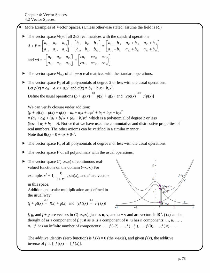
Chapter 4: Vector Spaces.
4.2 Vector Spaces.
p. 78
.
More Examples of Vector Spaces. (Unless otherwise stated, assume the field is R.)
The vector space M2,3of all 23 real matrices with the standard operations
A + B =
232221
131211
aaa
aaa +
232221
131211
bbb
bbb =
232322222121
131312121111
bababa
bababa
and cA = c
232221
131211
aaa
aaa =
232221
131211
cacaca
cacaca
The vector space Mm,n of all mn real matrices with the standard operations.
The vector space P2 of all polynomials of degree 2 or less with the usual operations.
Let p(x) = a0 + a1x + a2x2 and q(x) = b0 + b1x + b2x
2.
Define the usual operations (p + q)(x) def
p(x) + q(x) and (cp)(x) def
c[p(x)]
We can verify closure under addition:
(p + q)(x) = p(x) + q(x) = a0 + a1x + a2x2 + b0 + b1x + b2x
2
= (a0 + b0) + (a1 + b1)x + (a2 + b2)x2 which is a polynomial of degree 2 or less
(less if a2 + b2 = 0). Notice that we have used the commutative and distributive properties of
real numbers. The other axioms can be verified in a similar manner.
Note that 0(x) = 0 + 0x + 0x2.
The vector space Pn of all polynomials of degree n or less with the usual operations.
The vector space P of all polynomials with the usual operations.
The vector space C(–,) of continuous real-
valued functions on the domain (–,) For
example, x2 + 1,
21
8
x, sin(x), and e
x are vectors
in this space.
Addition and scalar multiplication are defined in
the usual way.
(f + g)(x) def
f(x) + g(x) and (cf )(x) def
c[f (x)]
f, g, and f + g are vectors in C(–,), just as u, v, and u + v and are vectors in Rn. f (x) can be
thought of as a component of f, just as ui is a component of u. u has n components: u1, u2, …,
un. f has an infinite number of components: …, f (–2), …, f (32 ), …, f (0), …, f ( ), ….
The additive identity (zero function) is f0(x) = 0 (the x-axis), and given f (x), the additive
inverse of f is [–f ](x) = –[ f (x)].

Chapter 4: Vector Spaces.
4.2 Vector Spaces.
p. 79
.
Another Example of a Vector Spaces
The vector space C[a, b] of continuous real-valued functions on the domain [a, b] over the
field R.
The most important reason for defining an abstract vector space using the ten axioms above is
that we can make general statements about all vector spaces. I.e. the same proof can be used for
Rn and for C[a, b].
Theorem 4.4 Properties of Vector Addition and Scalar Multiplication
Let v be a vector in Vn and let c be a scalar. Then
1) 0v = 0
2) c0 = 0
3) If cv = 0, then c = 0 or v = 0.
4) –1v = –v
Proof of (2): c0 = 0
c0 = 0 Given
c0 = c(0 + 0) Additive identity
c0 =
c0 + –( c0)
c0 + –( c0) =
0 = c0 Additive inverse
Proof of (3): If cv = 0, then c = 0 or c 0. If c 0, then
cv = c0 Given
c–1
cv = c–1
0 Multiply both sides by Multiplicative
inverse in R

Chapter 4: Vector Spaces.
4.2 Vector Spaces.
p. 80
.() V =
c(c–1
)v = c–1
0 Commutative property of multiplication
1v = c–1
0 Multiplicative inverse in R
v c–1
0 Scalar identity
v = 0 Theorem 4.3(2) – just proved
Thus, either c = 0 or v = 0.
Examples that are not Vector Spaces
Z2 (ordered pair of integers) over the field R. Z2
is not closed under scalar multiplication, for
example 21 (1, 2) = (
21 , 1) Z2
.
Aside on notation: 1 Z means “1 is an element of (is a member) of the set of integers.
21 Z means “1 is not an element of the set of integers.
Although Z2 satisfied Axioms 1–5 and 10 of a vector space, it is not a vector space because not
all axioms are satisfied.
The set of second-degree polynomials is not a vector space because it is not closed under
addition. For example, let p(x) = x2 and q(x) = –x
2 + x + 1. Then p(x) + q(x) = x + 1 is a first
degree polynomial.
Let V = R2 with the standard vector addition but nonstandard scalar multiplication defined by
c(u1, u2) = (cu1, 0). Show that V is not a vector space.
It turns out that the only axiom that is not satisfied in this case is (10) Scalar identity. For
example, 1(2, 3) = (2, 0) (2, 3).
opti
onal

Chapter 4: Vector Spaces.
4.2 Vector Spaces.
p. 81
.
Another Example that is not a Vector Spaces
Rotations in three dimensions represented as arrows using the right-hand rule.
The direction of the arrow represents the direction of the rotation, via
the right-hand rule, while the length of the arrow represents the
magnitude of the direction in degrees. Scalar multiplication is the
standard operation (stretching the arrow, or reversing the direction if
the scalar is negative). “Vector addition” (e.g. ) is the first rotation followed by
the second. This is not a vector space because “vector addition” is not commutative.
(In Chapter 6, we will see that rotations can be represented not as vectors, but as matrices.)
opti
onal


Chapter 4: Vector Spaces.
4.3 Subspaces of Vector Spaces.
p. 82
.() V =
.() V =
4.3 Subspaces of Vector Spaces.
Objective: Determine whether a subset W of a vector space V is a subspace of V.
Objective: Determine subspaces of Rn.
Many vector spaces are subspaces of larger spaces.
A nonempty subset W of a vector space V is a called a subspace of V when is a vector space
under the operations of vector addition and scalar multiplication defined in V.
Theorem 4.5 Test for a Subspace
If W is a nonempty subset of V, then W is a subspace of V if and only if the following
conditions hold.
0) W is not empty.
1) If u and v are in W, then u + v is in W. Closure under addition
2) If u is in W and c is a scalar, then cu is in W. Closure under scalar multiplication
Proof:
If W is a subspace of V, then W is a vector space satisfying the closure axioms, so
u + v is in W and cu is in W.
On the other hand, assume W is closed under vector addition and scalar multiplication. By
assumption, two axioms are satisfied.
1) u + v is in W. Closure under addition
6) cv is a vector in W. Closure under scalar multiplication
Then if u, v, and w are in W then they are also in V, so the following axioms are
automatically satisfied.
2) u + v = v + u Commutative property
3) (u + v) + w = u + (v + w) Associative property
7) c(u + v) = cu + cv Distributive property over vector addition
8) (c + d)u = cu + du Distributive property over scalar addition
9) c(du) = (cd)u Associative property
10) 1u = u Scalar identity
Because W is closed under scalar multiplication, we know that for any v in W, 0v and (–1)v
are also in W. From Thm. 4.4, we know that 0v = 0 and (–1)v = –v so the remaining axioms
are also satisfied.
4) W contains the zero vector 0. Additive identity
5) For every v in W, W contains –v. Additive inverse (opposite)

Chapter 4: Vector Spaces.
4.3 Subspaces of Vector Spaces.
p. 83
*
Examples of Subspaces and Sets that are not Subspaces.
Show that the set W = {(v1, 0, v3): v1 and v3 are real numbers} is a subspace
of R3 with the standard operations.
Graphically, W is the x-z plane in R3. W is nonempty, because it contains (0,
0, 0). W is closed under addition because if u, v W, then u + v = (u1, 0, u3)
+ (v1, 0, v3) = (u3 + v1, 0, u3 + v3) W. W is closed under scalar
multiplication because if c is a scalar and v W, then cv = c(v1, 0, v3) = (cv1,
0, cv3) W.
Is Z2 (ordered pair of integers) with the standard operations a subspace of
R2?
Z2 is closed under addition. But as we saw in 4.2, Z2
is not closed under
scalar multiplication, for example 21 (1, 2) = (
21 , 1) Z2
. So Z2 is not a
subspace of R2.
Show that the set W = {(v1, v2): v1 = 0 or v2 = 0} with the standard
operations is not a subspace of R2.
W is closed under scalar multiplication, but W is not closed under addition.
For example, (1, 0) + (0, 1) = (1, 1) W.
Is that the set W = {(v1, v2): v1 0 and v2 0} with the standard operations a
subspace of R2?
W is closed under addition, but W is not closed under scalar multiplication
when c < 0 and v 0. For example, (–1)(2, 3) = (–2, –3) W.
In general, a subspace is “straight” (line) or “flat” (plane or higher-dimensional object), is
“infinite” in all directions, has no “holes,” and contains the origin.
Let W be the set of all symmetric 22 matrices. Show that W is a subspace of M2,2 with the
standard operations.
“A is symmetric” means that A = AT. W is nonempty, because it contains
00
00. W is closed
under addition because if A, B W, then (A + B)T = A
T + B
T = A + B, so A + B is symmetric.
W is closed under scalar multiplication because if c is a scalar and A W, then (cA)T = c(A
T)
cA, so cA is symmetric.
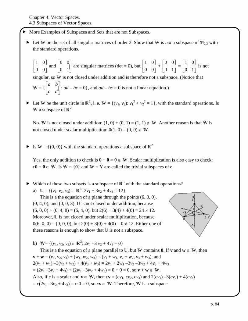
Chapter 4: Vector Spaces.
4.3 Subspaces of Vector Spaces.
p. 84
More Examples of Subspaces and Sets that are not Subspaces.
Let W be the set of all singular matrices of order 2. Show that W is not a subspace of M2,2 with
the standard operations.
00
01 and
10
00 are singular matrices (det = 0), but
00
01 +
10
00 =
10
01 is not
singular, so W is not closed under addition and is therefore not a subspace. (Notice that
W = {
dc
ba: ad – bc = 0}, and ad – bc = 0 is not a linear equation.)
Let W be the unit circle in R2, i. e. W = {(v1, v2): v1
2 + v2
2 = 1}, with the standard operations. Is
W a subspace of R2
No. W is not closed under addition: (1, 0) + (0, 1) = (1, 1) W. Another reason is that W is
not closed under scalar multiplication: 0(1, 0) = (0, 0) W.
Is W = {(0, 0)} with the standard operations a subspace of R2
Yes, the only addition to check is 0 + 0 = 0 W. Scalar multiplication is also easy to check:
c0 = 0 W. Is W = {0} and W = V are called the trivial subspaces of c.
Which of these two subsets is a subspace of R3 with the standard operations?
a) U = {(v1, v2, v3) R3: 2v1 + 3v2 + 4v3 = 12}
This is a the equation of a plane through the points (6, 0, 0),
(0, 4, 0), and (0, 0, 3). U is not closed under addition, because
(6, 0, 0) + (0, 4, 0) = (6, 4, 0), but 2(6) + 3(4) + 4(0) = 24 12.
Moreover, U is not closed under scalar multiplication, because
0(6, 0, 0) = (0, 0, 0), but 2(0) + 3(0) + 4(0) = 0 12. Either one of
these reasons is enough to show that U is not a subspace.
b) W= {(v1, v2, v3) R3: 2v1 –3 v2 + 4v3 = 0}
This is a the equation of a plane parallel to U, but W contains 0. If v and w W, then
v + w = (v1, v2, v3) + (w1, w2, w3) = (v1 + w1, v2 + w2, v3 + w3), and
2(v1 + w1) –3(v2 + w2) + 4(v3 + w3) = 2v1 + 2w1 –3v2 –3w2 + 4v3 + 4w3
= (2v1 –3v2 + 4v3) + (2w1 –3w2 + 4w3) = 0 + 0 = 0, so v + w W.
Also, if c is a scalar and v W, then cv = (cv1, cv2, cv3) and 2(cv1) –3(cv2) + 4(cv3)
= c(2v1 –3v2 + 4v3) = c·0 = 0, so cv W. Therefore, W is a subspace.

Chapter 4: Vector Spaces.
4.3 Subspaces of Vector Spaces.
p. 85
.() V =
More Example of Subspaces.
P[0, 1] is the set of all real-valued polynomial funtions on the domain [0, 1].
C1[0, 1] is the set of all real-valued, continuously differentiable functions on the domain [0, 1].
C0[0, 1], also written as C[0, 1], is the set of all real-valued, continuous functions on the
domain [0, 1].
Let W be the set of all real-valued, integrable functions on the interval [0, 1].
Let V be the set of all real-valued functions on the interval [0, 1].
If we take the usual definitions of vector addition and scalar multiplication, and we use R as
the field of scalars, then V is a vector space, and the other four sets are subspaces of V. In fact,
P[0, 1] is a subspace of C1[0, 1], which is is a subspace of C
0[0, 1], which is is a subspace of
W, which is is a subspace of V.
Theorem 4.6 The Intersection of Two Subspaces is a Subspace.
If V and W are both subspaces of a vector space U, then the interaction of V and W (denoted
V W) is also a subspace of U. (Note: V W is the set of all vectors that are in both V W.)
Proof:
Because V and W are both subspaces of U, we know that they both
contain 0, so V W contains 0 and is not empty. To show that
V W is closed under addition, let u1 and u2 be two vectors in
V W. Because u1 and u2 are both in V, and—being a subspace—V
is closed, u1 + u2 is also in V. Likewise, u1 + u2 is also in W. Since
u1 + u2 is in both V and W, u1 + u2 is in V W, so V W is closed
under vector addition. A similar argument shows that V W is
closed under scalar multiplication, so V W is a subspace of U.
U
V
W
V W

Chapter 4: Vector Spaces.
4.4 Spanning Sets and Linear Independence.
p. 86
4.4 Spanning Sets and Linear Independence.
Objective: Write a vector as a linear combination of other vectors in a vector space V.
Objective: Determine whether a spanning set S of vectors in a vector space is a spanning set of
V.
Objective: Determine whether a set of vectors in a vector space V is linearly independent.
Objective: Prove results about spanning sets and linear independence.
A vector v in a vector space V is called a linear combination of the vectors u1, u2, …, uk in V if
and only if v can be written in the form
v = c1u1 + c2u2 + … + ckuk
where c1, c2, …, ck are scalars.
Example: Write the vector v = (–1, –2, 2) as a linear combination of the vectors in the set
S = {(2, –1, 3), (5, 0, 4)} (if possible).
Solution: We need to solve v = c1u1 + c2u2 for the scalars ci. Substituting in the given vectors, we
have
(–1, –2, 2) = c1(2, –1, 3) + c2(5, 0, 4)
(–1, –2, 2) = (2c1, –1c1, 3c1) + (5c2, 0c2, 4c2)
(–1, –2, 2) = (2c1 + 5c2, –1c1 + 0c2, 3c1 + 4c2)
which gives the system
243
201
152
21
21
21
cc
cc
cc
or
2
2
1
43
01
62
2
1
c
c
Solve this system by finding the reduced row-echelon form (using software)
243
201
162
000
110
201
or
0
1
2
00
10
01
2
1
c
c so c1 = 2 and c2 = –1.
Answer: (–1, –2, 2) = 2(2, –1, 3) – 1(5, 0, 4).
Example: Write the vectors v = (–3, 15, 18) and w = (31 ,
34 ,
21 ) as linear combinations of the
vectors in the set S = {(2, 0, 7), (2, 4, 5), (2, –12, 13)} (if possible).
Solution: We need to solve

Chapter 4: Vector Spaces.
4.4 Spanning Sets and Linear Independence.
p. 87
.
Example: Write the vector v =
2057
4824 as linear combinations of the vectors in the set
S = {
45
21,
26
72,
1211
94,
54
56} (if possible).
Solution:
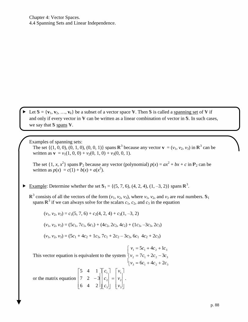
Chapter 4: Vector Spaces.
4.4 Spanning Sets and Linear Independence.
p. 88
Let S = {v1, v2, …, vk} be a subset of a vector space V. Then S is called a spanning set of V if
and only if every vector in V can be written as a linear combination of vector in S. In such cases,
we say that S spans V.
Examples of spanning sets:
The set {(1, 0, 0), (0, 1, 0), (0, 0, 1)} spans R3 because any vector v = (v1, v2, v3) in R3
can be
written as v = v1(1, 0, 0) + v2(0, 1, 0) + v3(0, 0, 1).
The set {1, x, x2} spans P2 because any vector (polynomial) p(x) = ax
2 + bx + c in P2 can be
written as p(x) = c(1) + b(x) + a(x2).
Example: Determine whether the set S1 = {(5, 7, 6), (4, 2, 4), (1, –3, 2)} spans R3.
R3 consists of all the vectors of the form (v1, v2, v3), where v1, v2, and v3 are real numbers. S1
spans R3 if we can always solve for the scalars c1, c2, and c3 in the equation
(v1, v2, v3) = c1(5, 7, 6) + c2(4, 2, 4) + c3(1, –3, 2)
(v1, v2, v3) = (5c1, 7c1, 6c1) + (4c2, 2c2, 4c2) + (1c3, –3c3, 2c3)
(v1, v2, v3) = (5c1 + 4c2 + 1c3, 7c1 + 2c2 – 3c3, 6c1 4c2 + 2c3)
This vector equation is equivalent to the system
3213
3212
3211
246
327
145
cccv
cccv
cccv
or the matrix equation
3
2
1
3
2
1
246
327
145
v
v
v
c
c
c
.

Chapter 4: Vector Spaces.
4.4 Spanning Sets and Linear Independence.
p. 89
This equation can always be solved for c1, c2, and c3, because 0
246
327
145
, so the matrix is
invertible. (To be precise, the determinant is –32.) Therefore, S1 spans R3.
Example: Determine whether the set S2 = {(5, 7, 6), (3, 2, 4), (1, –3, 2)} spans R3.
only this number has changed.
Solution:
Geometrically, the vectors in S2 all lie in the same plane (a “2-dimensional” object), while the
vectors in S1 do not. We need a “3-dimensional” space to contain S1.
S1 S2.

Chapter 4: Vector Spaces.
4.4 Spanning Sets and Linear Independence.
p. 90
*
If S = {v1, v2, …, vk} is a set of vectors in a vector space V, then the span of S is the set of all
linear combinations of the vectors in S.
span(S) = {c1v1 + c2v2 + …+ ckvk: c1, c2, … ck, are scalars}
We sometimes write span{v1, v2, …, vk} instead of span(S).
Another notation for span(S)—which we will avoid because it will be confusing later—is
v1, v2, …, vk.
Theorem 4.7 Span(S) is a Subspace of V
If S = {v1, v2, …, vk} is a set of vectors in a vector space V, then span(S) is a subspace of V.
Moreover, span(S) is the smallest subspace of V that contains (S), in the sense that every
subspace that contains S must also contain span(S).
Proof
First, we want to show that span(S) is a subspace of V.
So we need to show that
Let c be a scalar and let u and w be any vectors in span(S). Then
Next, we want to show that every subspace that contains S must also contain span(S). This is
Lab Problem 4.4.55.

Chapter 4: Vector Spaces.
4.4 Spanning Sets and Linear Independence.
p. 91
Sometimes, one vector can be written “in terms of” other vectors. For example, in S2 = {(5, 7, 6),
(3, 2, 4), (1, –3, 2)} from above, (3, 2, 4) = 2
)2,3,1()6,7,5( . We could say that (3, 2, 4) “is
dependent” upon (5, 7, 6) and (1, –3, 2). But we could just as easily solve for (5, 7, 6); there is
no good reason to treat (3, 2, 4) as special. A more equitable equation is
1(5, 7, 6) – 2(3, 2, 4) + 1(1, –3, 2) = (0, 0, 0).
In fact, there are an infinite number of solutions to c1(5, 7, 6) + c2(3, 2, 4) + c3(1, –3, 2) = 0.
c1 = t, c2 = –2t, c3 = t. (This includes c1 = c2 = c3 = 0.)
On the other hand, for S1 = {(5, 7, 6), (4, 2, 4), (1, –3, 2)}, the only solution to
c1(5, 7, 6) + c2(4, 2, 4) + c3(1, –3, 2) = (0, 0, 0) or
0
0
0
246
327
145
3
2
1
c
c
c
is
0
0
0
0
0
0
246
327
1451
3
2
1
c
c
c
. This is called the trivial solution.
If S = {v1, v2, …, vk} is a set of vectors in a vector space V, then S is called linearly independent
if and only if the equation
c1v1 + c2v2 + …+ ckvk = 0
has only the trivial solution c1 = c2 = …= ck = 0. S is called linearly dependent if and only if
there are also nontrivial solutions.
Examples #1-4: Let w1 = (7, 3, –5), w2 = (1, 4, 6), w3 = (9, 11, 7), w4 = (12, –5, –4), and
w5 = (–6, 5, 8).
Example #1: Is {w1, w2} linearly independent? Does {w1, w2} span R3?
Solution:
To decide linear independence, we want to solve c1w1 + c2w2 = 0.
To decide spanning R3, we want to solve c1w1 + c2w2 = (v1, v2, v3) for arbitrary v1, v2, and v3.
Both equations look like c1(7, 3, –5) + c2(1, 4, 6) = (v1, v2, v3).
(For linear independence, the right-hand side is v1 = v2 = v3 = 0.)
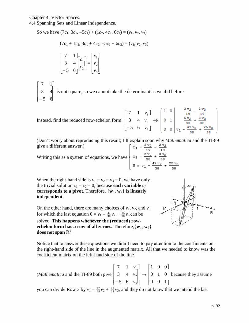
Chapter 4: Vector Spaces.
4.4 Spanning Sets and Linear Independence.
p. 92
So we have (7c1, 3c1, –5c1) + (1c2, 4c2, 6c2) = (v1, v2, v3)
(7c1 + 1c2, 3c1 + 4c2, –5c1 + 6c2) = (v1, v2, v3)
3
2
1
2
1
65
43
17
v
v
v
c
c
65
43
17
is not square, so we cannot take the determinant as we did before.
Instead, find the reduced row-echelon form:
3
2
1
65
43
17
v
v
v
(Don’t worry about reproducing this result; I’ll explain soon why Mathematica and the TI-89
give a different answer.)
Writing this as a system of equations, we have
When the right-hand side is v1 = v2 = v3 = 0, we have only
the trivial solution c1 = c2 = 0, because each variable ci
corresponds to a pivot. Therefore, {w1, w2} is linearly
independent.
On the other hand, there are many choices of v1, v2, and v3
for which the last equation 0 = v1 – 3847 v2 +
3825 v3 can be
solved. This happens whenever the (reduced) row-
echelon form has a row of all zeroes. Therefore,{w1, w2}
does not span R3.
Notice that to answer these questions we didn’t need to pay attention to the coefficients on
the right-hand side of the line in the augmented matrix. All that we needed to know was the
coefficient matrix on the left-hand side of the line.
(Mathematica and the TI-89 both give
3
2
1
65
43
17
v
v
v
100
010
001
because they assume
you can divide Row 3 by v1 – 3847 v2 +
3825 v3, and they do not know that we intend the last

Chapter 4: Vector Spaces.
4.4 Spanning Sets and Linear Independence.
p. 93
column to be on the right-hand side of the equation. However, the right-hand column is not
important to deciding linear independence and spanning.)
Example #2: Is {w1, w2, w3} linearly independent? Does {w1, w2, w3} span R3?
Solution:
To decide linear independence, we want to solve c1w1 + c2w2 + c3w3 = 0.
To decide spanning R3, we want to solve c1w1 + c2w2 + c3w3 = v for arbitrary v.
Using block multiplication notation, we write [ w1 | w2 | w3 ]
3
2
1
c
c
c
=
3
2
1
v
v
v
so
765
1143
917
3
2
1
c
c
c
=
3
2
1
v
v
v
.
765
1143
917
is singular (not invertible) because its
determinant (found using software) is zero. This tells us that
sometimes we cannot solve c1w1 + c2w2 + c3w3 = v, so {w1,
w2, w3} does not span R3. This also tells us that c1w1 + c2w2 + c3w3 = 0 has an infinite number
of solutions, so {w1, w2, w3} is linearly dependent.
For another perspective, the reduced row-echelon form of
765
1143
917
is
000
210
101
.
To investigate linear independence, we set the right-hand side equal to zero. The third column
in the matrix, which doesn’t have a pivot, gives us a free parameter. (Fewer pivots than
variables.)
0000
0210
0101
321
321
321
ccc
ccc
ccc
has the solutions
tc
tc
tc
1
2
3
2 where t is a free parameter.
Since we have non-trivial solutions, {w1, w2, w3} is linearly dependent.
To investigate spanning, we set the right-hand side equal to arbitrary numbers. The third row of
all zeroes in the matrix gives us 0c1 + 0c2 + 0c3 = #, which does not have a solution when the
right-hand side is not zero. (Fewer pivots than equations.) Therefore, {w1, w2, w3} does not
span R3.
Example #3: Is {w1, w2, w4} linearly independent? Does {w1, w2, w4} span R3?
Solution:
To decide linear independence, we want to solve c1w1 + c2w2 + c4w4 = 0.
To decide spanning R3, we want to solve c1w1 + c2w2 + c4w4 = v for arbitrary v.
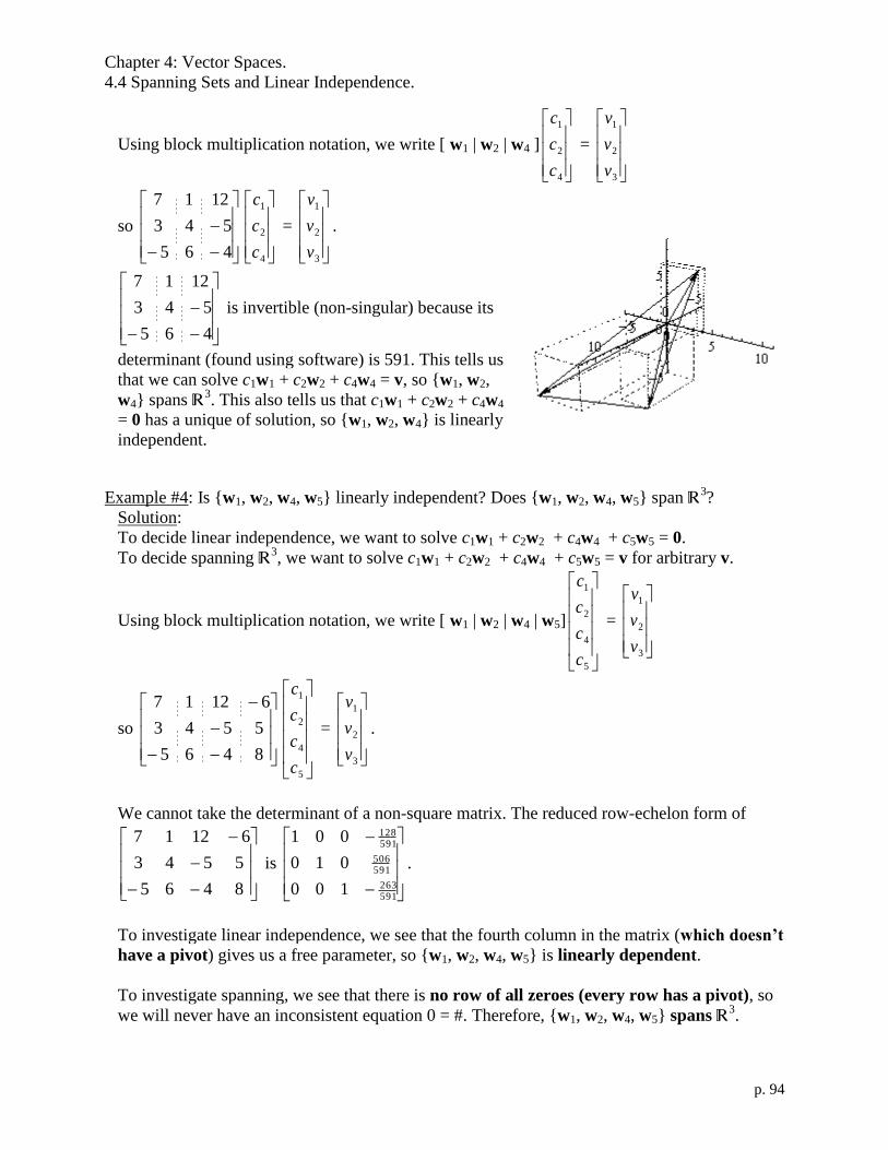
Chapter 4: Vector Spaces.
4.4 Spanning Sets and Linear Independence.
p. 94
Using block multiplication notation, we write [ w1 | w2 | w4 ]
4
2
1
c
c
c
=
3
2
1
v
v
v
so
465
543
1217
4
2
1
c
c
c
=
3
2
1
v
v
v
.
465
543
1217
is invertible (non-singular) because its
determinant (found using software) is 591. This tells us
that we can solve c1w1 + c2w2 + c4w4 = v, so {w1, w2,
w4} spans R3. This also tells us that c1w1 + c2w2 + c4w4
= 0 has a unique of solution, so {w1, w2, w4} is linearly
independent.
Example #4: Is {w1, w2, w4, w5} linearly independent? Does {w1, w2, w4, w5} span R3?
Solution:
To decide linear independence, we want to solve c1w1 + c2w2 + c4w4 + c5w5 = 0.
To decide spanning R3, we want to solve c1w1 + c2w2 + c4w4 + c5w5 = v for arbitrary v.
Using block multiplication notation, we write [ w1 | w2 | w4 | w5]
5
4
2
1
c
c
c
c
=
3
2
1
v
v
v
so
8465
5543
61217
5
4
2
1
c
c
c
c
=
3
2
1
v
v
v
.
We cannot take the determinant of a non-square matrix. The reduced row-echelon form of
8465
5543
61217
is
591263
591506
591128
100
010
001
.
To investigate linear independence, we see that the fourth column in the matrix (which doesn’t
have a pivot) gives us a free parameter, so {w1, w2, w4, w5} is linearly dependent.
To investigate spanning, we see that there is no row of all zeroes (every row has a pivot), so
we will never have an inconsistent equation 0 = #. Therefore, {w1, w2, w4, w5} spans R3.

Chapter 4: Vector Spaces.
4.4 Spanning Sets and Linear Independence.
p. 95
*
*
Summary:
{w1, …, wk} in Rn is linearly independent if and only if the reduced row-echelon form of the
matrix [w1 | … | wk ] has as many pivots as columns (variables).
{w1, …, wk} spans Rn if and only if the reduced row-echelon form of the matrix
[w1 | … | wk ] has as many pivots as rows (equations), i.e. no rows of all zeroes.
Theorem 4.8 A Property of Linearly Dependent Sets
A set S = {v1, v2, …, vk}, k 2, is linearly dependent if and only if at least one of the vectors vj
can be written as a linear combination of the other vectors in S.
Proof
To prove “only if (),” assume set S is linearly dependent and k 2.
Then
Because one of the coefficients must be nonzero, we can assume without loss of generality
(WOLOG) that c1 0. Then
Conversely (which means changing to ), suppose v1 is a linear combination of the other
vectors in S. Then
v1 =
0 =
Thus, {v1, v2, …, vk} is linearly dependent because
Example: Given that {w1, w2, w4, w5} is linearly dependent, and that
c1w1 + c2w2 + c4w4 + c5w5 = 0 has the solutions
tc
tc
tc
tc
509128
2
509506
2
509263
4
5
, write w2 as a linear
combination of the other vectors in the set.

Chapter 4: Vector Spaces.
4.4 Spanning Sets and Linear Independence.
p. 96
*
*
Solution:
509128 tw1 –
509506 tw2 +
509263 tw4 + tw5 = 0
so 128w1 + 263w4 + 509w5 = 506w2
so w2 = 506128 w1 +
506263 w4 +
506509 w5
Theorem 4.9 Corollary
Two vectors v1 and v2 in a vector space V are linearly dependent if and only if one is a scalar
multiple of the other.
Proof: From the proof of Theorem 4.8,
Theorem
Any set S = {0, v1, v2, …, vk}, containing the zero vector is linearly dependent.
Proof: 10 + 0v1 + 0v2 + … + 0vk = 0.
Since not all coefficients are zero, S is linearly dependent.


Chapter 4: Vector Spaces.
4.5 Basis and Dimension.
p. 97
4.5 Basis and Dimension.
Objective: Recognize bases in the vector spaces Rn, Pn, and Mm,n.
Objective: Find the dimension of a vector space.
Objective: Prove results about spanning sets and linear independence.
A set of vectors S = {v1, v2, …, vk} in a vector space V is called a basis for V when
1) S spans V, and
2) S is linearly independent.
“S spans V” says that the set S is not too small to be a basis; “S is linearly independent” says
that the set S is not too big to be a basis. (The plural of “basis” is “bases.”)
In the diagram on the left, you can see that S1 = {u1, u2} is too small to span R3. For example, v
is outside of span(S1). In the figure on the right, you can see that S1 = {u1, u2, u3} is large
enough to span R3. For example, you can see the linear combination that gives v. Finally, In the
figure on the right, you can see that S3 = {u1, u2, u3, v} is large to be linearly independent,
because v is a linear combination of u1, u2, and u3.

Chapter 4: Vector Spaces.
4.5 Basis and Dimension.
p. 98
*
*
Example. The standard basis for R3: Show that {(1, 0, 0), (0, 1, 0), (0 0, 1)} is a basis for R3
.
Solution:
To decide linear independence, we want to solve c1(1, 0, 0) + c2(0, 1, 0) + c3(0 0, 1) = 0.
To decide spanning R3, we want to solve c1(1, 0, 0) + c2(0, 1, 0) + c3(0 0, 1) = v for arbitrary v.
These equations are
100
010
001
3
2
1
c
c
c
=
0
0
0
and
100
010
001
3
2
1
c
c
c
=
3
2
1
v
v
v
The first equation has only the trivial solution, and the second equation always has a solution, so
{(1, 0, 0), (0, 1, 0), (0 0, 1)}is linearly independent and it spans R3. Therefore, {(1, 0, 0),
(0, 1, 0), (0 0, 1)} is a basis for R3.
The standard basis in Rn is
1,,0,0
0,,1,0
0,,0,1
2
1
ne
e
e
Example: Show that {(7, –2, 5), (–3, –9, –1), (1, 7, –7)} is a basis for R3.
Solution:
To decide linear independence, we want to solve
.
To decide spanning R3, we want to solve
As matrix equations, we obtain
The matrix is invertible (its determinant is 474). Because of this, the first equation has only the
trivial solution, and the second equation always has a solution, so {(7, –2, 5), (–3, –9, –1),
(1, 7, –7)} is linearly independent and it spans R3. Therefore, {(7, –2, 5), (–3, –9, –1),
(1, 7, –7)} is a basis for R3.

Chapter 4: Vector Spaces.
4.5 Basis and Dimension.
p. 99
*
The standard basis for Pn is {1, x, x2, …, x
n}.
The standard basis for M2,3 is {
00
00
01
,
00
00
10
,
00
01
00
,
00
10
00
,
01
00
00
,
10
00
00
}.
Theorem 4.9 Uniqueness of a Basis Representation
If S = {v1, v2, …, vk} is a basis for a vector space V, then every vector in V, can be written in
one and only one way as a linear combination of vectors in S.
Proof: Let u be an arbitrary vector in V,
u can be written in at least one way as a linear combination of vectors in S because
Now suppose that u can be written as a linear combination of vectors in S in two ways:
u = b1v1 + b2v2 + …+ bkvk and u = c1v1 + c2v2 + …+ ckvk
Subtracting these two equations gives
Since S is linearly independent,
Thus, u can be written as a linear combination of vectors in S in only one way.
Example: Using the basis {(7, –2, 5), (–3, –9, –1), (1, 7, –7)} for R3 from the previous example,
find the unique representation of u = (u1, u2, u3) using this basis. In other words, find the unique
solution for the constants c1, c2, c3 in the equation
u = c1(7, –2, 5), + c2(–3, –9, –1), + c3(1, 7, –7)}

Chapter 4: Vector Spaces.
4.5 Basis and Dimension.
p. 100
Solution: As a matrix equation, we obtain
Lemma 4.9½ Dimension of Spanning Sets and Linearly Independent Sets
If S1 = {v1, v2, …, vn} spans a vector space V and S2 = {u1, u2, …, um} is a set of m linearly
independent vectors in V, then m n.
Proof by contradiction:
Suppose m > n. To show that S2 is linearly dependent (a contradiction), we need to find scalars
k1, k1, …, km (not all zero) such that
k1u1 + k2u2 + … + kmum =
1
1
11
mm
mmkk
u
u
= 0
Because S1 spans V, each ui is a linear combination of vectors in S1:
1
1
1
1
nn
nm
mm
C
v
v
u
u
i.e.
nmnmm
nn
CC
CC
vvu
vvu
...
...
11
11111
Substituting into the first equation gives
1
1
11
nn
nmmm Ckk
v
v
= 0
Now consider
11
1
0
0
][
nmm
mn
T
k
k
C
This is n equations for m unknowns (ki), with n < m, so we have (infinitely many) nontrivial
(non-zero) solutions (k1, k2, …, km). Taking the transpose, we have a non-zero solution to

Chapter 4: Vector Spaces.
4.5 Basis and Dimension.
p. 101
*
*
*
n1
00 = nmmn Ckk 11
Therefore, we have a non-zero solution to
0 =
1
1
11
nn
nmmm Ckk
v
v
=
1
1
11
mm
mmkk
u
u
This says that S2 = {u1, u2, …, um} is linearly dependent, which contradicts the premise, thus
completing the proof by contradiction.
Theorem 4.10 Bases and Linear Dependence
If S = {v1, v2, …, vn} is a basis for a vector space V,
then every set containing more than n vectors in linearly dependent.
Proof:
S = {v1, v2, …, vn} spans V so by Lemma 4.9½, any set of m linearly independent vectors in V
has m n. Therefore, any set of m vectors in V where m > n must be linearly dependent.
Note: the last step is true because “P Q” is logically equivalent to its contrapositive “(not Q)
(not P)”.
Theorem 4.11 Bases and Linear Dependence
If a vector space V has one basis with n vectors, then every basis for V has n vectors.
Proof:
Let S1 = {u1, u2, …, un} be one basis for Vand let S2 = {v1, v2, …, vm} be another basis for V.
Because S1 is a basis, and S2 is linearly independent, Thm. 4.10 tells us that m < n. Similarly,
because S2 is a basis, and S1 is linearly independent, Thm. 4.10 tells us that n < m. Therefore,
m = n.
If a vector space V has basis consisting of n vectors, then the number n is called the dimension of
V, denoted by dim(V) = n. We define the dimension of the trivial vector space {0} to be n = 0.
The dimension of a vector space is well-defined (unambiguous) because of Thm. 4.11.

Chapter 4: Vector Spaces.
4.5 Basis and Dimension.
p. 102
.
Examples:
dim(Rn) = n
dim(Pn) = n + 1
dim(Mm,n) = mn
Example: Find the dimension of the subspace of R3 given by W= {(2a, a –3b, a + b): a and b are
real numbers}.
Solution:We can write (2a, a –3b, a + b) = a(2, 1, 1) + b(0, –3, 1), so W is spanned by S =
{(2, 1, 1), (0, –3, 1)}. Moreover, S is linearly independent, because the reduced row echelon
form of
11
31
02
is
00
10
01
(every column has a pivot). The only solution to
00
10
01
b
a =
0
0
0
is a = b = 0. So S is a basis, and dim(W) = 2.
Example: Find the dimension of the subspace W of P4 spanned by
S = {–3 – 5x + x2 + 2x
4,
–5x – 4x2 + 4x
3,
–12 – 10x + 11x2 – 12x
3 + 11x
4,
3 + 10x + 4x2 – 5x
4}
Solution: S spans W, but it might not be linearly independent. To decide linear independence, we
solve
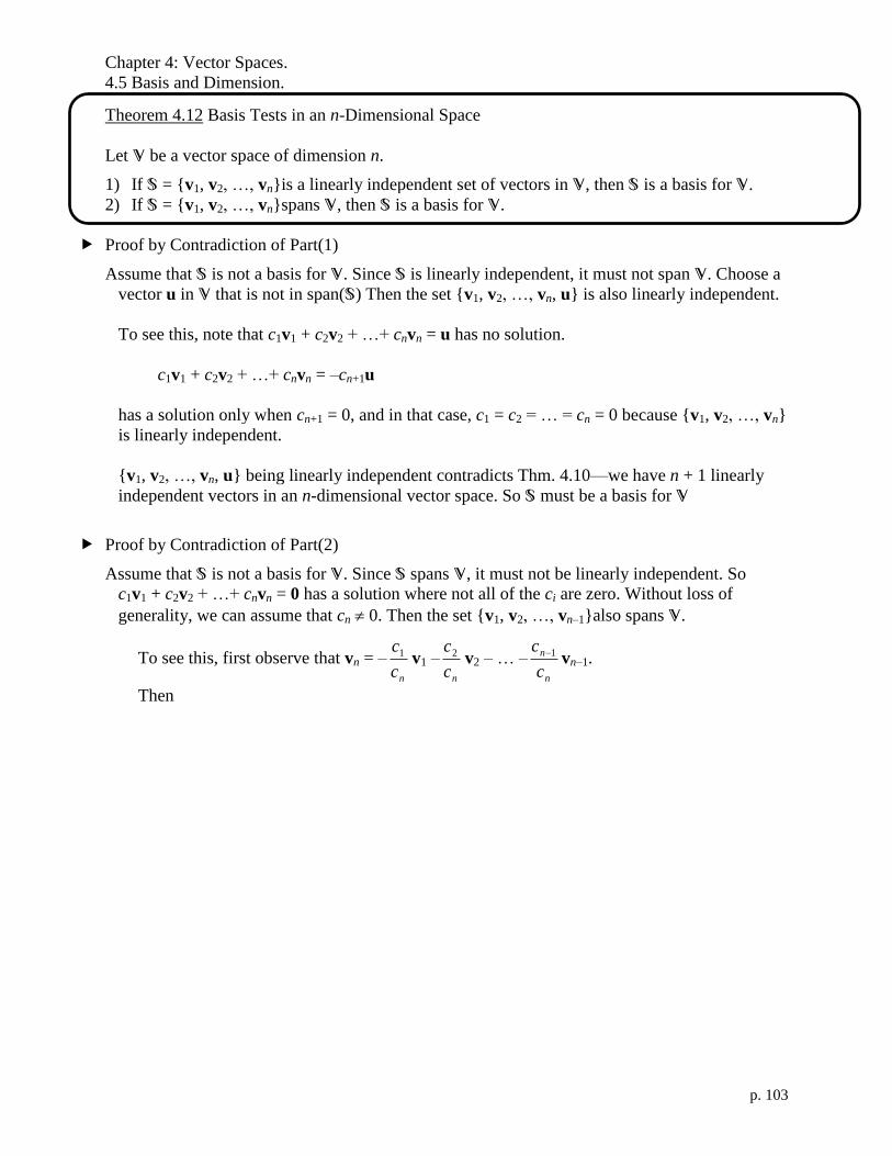
Chapter 4: Vector Spaces.
4.5 Basis and Dimension.
p. 103
*
Theorem 4.12 Basis Tests in an n-Dimensional Space
Let V be a vector space of dimension n.
1) If S = {v1, v2, …, vn}is a linearly independent set of vectors in V, then S is a basis for V.
2) If S = {v1, v2, …, vn}spans V, then S is a basis for V.
Proof by Contradiction of Part(1)
Assume that S is not a basis for V. Since S is linearly independent, it must not span V. Choose a
vector u in V that is not in span(S) Then the set {v1, v2, …, vn, u} is also linearly independent.
To see this, note that c1v1 + c2v2 + …+ cnvn = u has no solution.
c1v1 + c2v2 + …+ cnvn = –cn+1u
has a solution only when cn+1 = 0, and in that case, c1 = c2 = … = cn = 0 because {v1, v2, …, vn}
is linearly independent.
{v1, v2, …, vn, u} being linearly independent contradicts Thm. 4.10—we have n + 1 linearly
independent vectors in an n-dimensional vector space. So S must be a basis for V
Proof by Contradiction of Part(2)
Assume that S is not a basis for V. Since S spans V, it must not be linearly independent. So
c1v1 + c2v2 + …+ cnvn = 0 has a solution where not all of the ci are zero. Without loss of
generality, we can assume that cn 0. Then the set {v1, v2, …, vn–1}also spans V.
To see this, first observe that vn = –nc
c1 v1 –nc
c2 v2 – … –n
n
c
c 1 vn–1.
Then

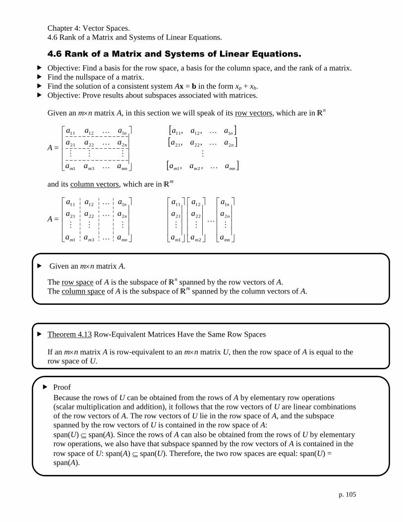
Chapter 4: Vector Spaces.
4.6 Rank of a Matrix and Systems of Linear Equations.
p. 105
.(
.(
4.6 Rank of a Matrix and Systems of Linear Equations.
Objective: Find a basis for the row space, a basis for the column space, and the rank of a matrix.
Find the nullspace of a matrix.
Find the solution of a consistent system Ax = b in the form xp + xh.
Objective: Prove results about subspaces associated with matrices.
Given an mn matrix A, in this section we will speak of its row vectors, which are in Rn
A =
mnmm
n
n
aaa
aaa
aaa
31
22221
11211
mnmm
n
n
aaa
aaa
aaa
,,
,,
,,
21
22221
11211
and its column vectors, which are in Rm
A =
mnmm
n
n
aaa
aaa
aaa
31
22221
11211
mn
n
n
mm a
a
a
a
a
a
a
a
a
2
1
2
22
12
1
21
11
Given an mn matrix A.
The row space of A is the subspace of Rn spanned by the row vectors of A.
The column space of A is the subspace of Rm spanned by the column vectors of A.
Theorem 4.13 Row-Equivalent Matrices Have the Same Row Spaces
If an mn matrix A is row-equivalent to an mn matrix U, then the row space of A is equal to the
row space of U.
Proof
Because the rows of U can be obtained from the rows of A by elementary row operations
(scalar multiplication and addition), it follows that the row vectors of U are linear combinations
of the row vectors of A. The row vectors of U lie in the row space of A, and the subspace
spanned by the row vectors of U is contained in the row space of A:
span(U) span(A). Since the rows of A can also be obtained from the rows of U by elementary
row operations, we also have that subspace spanned by the row vectors of A is contained in the
row space of U: span(A) span(U). Therefore, the two row spaces are equal: span(U) =
span(A).

Chapter 4: Vector Spaces.
4.6 Rank of a Matrix and Systems of Linear Equations.
p. 106
.(
Theorem 4.14 Basis for the Row Space of a Matrix
If a matrix A is row-equivalent to a matrix U in row-echelon form, the then the nonzero row
vectors of U form a basis for the row space of A.
Example: Show that the nonzero rows of
00000
10000
31000
26410
34291
(a matrix in row-echelon form)
are linearly independent.
Solution: We want to solve 00000 =
10000
31000
26410
34291
4
3
2
1
c
c
c
c
The first column of the right-hand side sum is c1, so c1 = 0. The second column of the right-
hand side sum is –9c1 + c2 = 0 + c2, so c2 = 0. The fourth column of the right-hand side sum is
0 + 0 + c3 (because c1 = c2 = 0), so c3 = 0. Finally, the fifth column of the right-hand side sum
is 0 + 0 + 0 + c4 (because c1 = c2 = c3 = 0), so c4 = 0. Therefore the nonzero rows are linearly
independent.
Alternate Solution: The transpose of 00000 =
10000
31000
26410
34291
4
3
2
1
c
c
c
c
is
0
0
0
0
0
= c1 1
3
4
2
9
1
+ c2
2
6
4
1
0
+ c3
3
1
0
0
0
+ c4
1
0
0
0
0
=
1323
0164
0042
0019
0001
4
3
2
1
c
c
c
c
.
Solving this by “forward substitution” (first row down to the last row) yields
4
3
2
1
c
c
c
c
=
0
0
0
0
.

Chapter 4: Vector Spaces.
4.6 Rank of a Matrix and Systems of Linear Equations.
p. 107
Example: Find a basis for the row space of
303240
52113769
4576374
2244334
4981
Solution: The row-echelon form is
0000
0000
1000
6810
4981
, so a basis for the row space is
{[1, –8, –9, 4], [0, 1, 8, –6], [0, 0, 0, 1]}.
You could also take the reduced row-echelon form
0000
0000
1000
0810
05501
to obtain the basis
{[1, 0, 55, 0], [0, 1, 8, 0], [0, 0, 0, 1]}.
Example: Find a basis for the subspace of R3 spanned by {[1, –6, 3], [1, –5, 7], [–7, 38, –37]}.
Solution:
Lemma: The pivot columns of a matrix U in row-echelon form (or reduced row-echelon form)
are linearly independent.

Chapter 4: Vector Spaces.
4.6 Rank of a Matrix and Systems of Linear Equations.
p. 108
.(
Example: U =
0000000
100000
1000
100
1
x
xxx
xxxx
xxxxxx
. If we look only at the pivot columns and solve
0000
1000
100
10
1
x
xx
xxx
4
3
2
1
c
c
c
c
=
0
0
0
0
0
, we see by back substitution that the unique solution is
4
3
2
1
c
c
c
c
=
0
0
0
0
, so the pivot columns of U are linearly independent.
Lemma: The pivot columns of a matrix U in row-echelon form (or reduced row-echelon form)
span the column space of U.
Example: U =
0000000
100000
1000
100
1
x
xxx
xxxx
xxxxxx
. The column space of U is the subset of R5 consisting
of vectors whose fifth component is zero (because we are taking linear combinations of vectors
whose fifth component is zero).
If we look only at the pivot columns, we can always solve
0000
1000
100
10
1
x
xx
xxx
4
3
2
1
c
c
c
c
=
0
4
3
2
1
v
v
v
v
, by back
substitution so the pivot columns of U span the column space of U.
Theorem Basis for the Column Space of a Matrix
Given an mn matrix A and its row-echelon (or reduced row-echelon) form U. Then the columns
of A that correspond to the pivot columns of U form a basis for the column space of A.
Proof: by combining the two preceding lemmas, we know that the pivot columns of U form a
basis for the column space of U. Let ai be the column vectors of A and ui be the column
vectors of U, so A = [a1| …| an ] and U = [u1| …| un ]. We can factor PA = LU, so Pai = Lui
for each column vector,
ui = L–1
Pai, and ai = P–1
Lui. (essential idea)
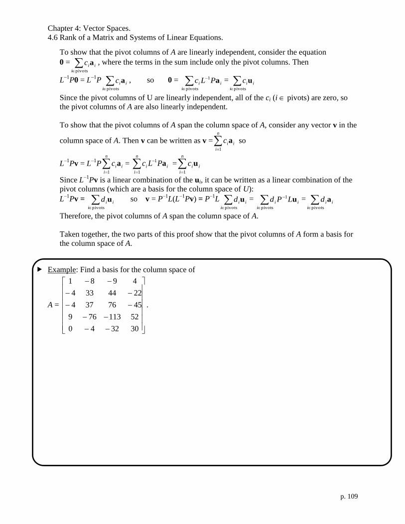
Chapter 4: Vector Spaces.
4.6 Rank of a Matrix and Systems of Linear Equations.
p. 109
.(
To show that the pivot columns of A are linearly independent, consider the equation
0 = pivotsi
iic a , where the terms in the sum include only the pivot columns. Then
L–1
P0 = L–1
P pivotsi
iic a , so 0 =
pivots
1
i
ii PLc a = pivotsi
iic u
Since the pivot columns of U are linearly independent, all of the ci (i pivots) are zero, so
the pivot columns of A are also linearly independent.
To show that the pivot columns of A span the column space of A, consider any vector v in the
column space of A. Then v can be written as v =
n
i
iic1
a so
L–1
Pv = L–1
P
n
i
iic1
a =
n
i
ii PLc1
1a =
n
i
iic1
u
Since L–1
Pv is a linear combination of the ui, it can be written as a linear combination of the
pivot columns (which are a basis for the column space of U):
L–1
Pv = pivotsi
iid u so v = P–1
L(L–1
Pv) = P–1
L pivotsi
iid u =
pivots
1
i
ii LPd u = pivotsi
iid a
Therefore, the pivot columns of A span the column space of A.
Taken together, the two parts of this proof show that the pivot columns of A form a basis for
the column space of A.
Example: Find a basis for the column space of
A =
303240
52113769
4576374
2244334
4981
.

Chapter 4: Vector Spaces.
4.6 Rank of a Matrix and Systems of Linear Equations.
p. 110
.(
.(
.(
Theorem 4.15 Row Space and Column Space have the Same Dimension.
If A is an mn matrix, then the row space and column space of A have the same dimension.
Proof: The dimension of the row space and the dimension of the column space are both equal to
the number of pivots in the row-echelon form (or in the reduced row echelon form) of A.
The rank r = rank(A) of a matrix is the dimension of its row space, the dimension of its column
space, and the number of pivots in the row-echelon form (or in the reduced row echelon form).
Theorem 4.16 Solutions to a Homogeneous System Ax = 0
If A is an mn matrix, then the set of all solutions to the homogeneous system of linear equations
Ax = 0 is a subspace of Rn.
Proof: Because A is mn, x is n1, so the set of all solutions to the homogeneous system of
linear equations Ax = 0 is a subset of Rn. We will call this subset N. N is not empty because it
contains 0: A0 = 0. Now we must show …
If A is an mn matrix, the subspace of Rn consisting of all solutions to the homogeneous system
Ax = 0 is a called the nullspace of A and is denoted by N(A). We sometimes call N(A) the
solution space of Ax = 0. The dimension of N(A) is called the nullity of A, and is sometimes
written as (the Greek letter nu).

Chapter 4: Vector Spaces.
4.6 Rank of a Matrix and Systems of Linear Equations.
p. 111
.(
Theorem 4.17+ Solutions of a Homogeneous System Ax = 0
If A is an mn matrix of rank r and nullity , then the dimension of the solution space of Ax = 0,
i.e. N(A), is = n – r. That is, n = rank(A) + nullity(A), or the number of variables = number of
pivot variables + number of free variables.
Moreover, the solution set to the homogeneous system Ax = 0 is the same as the solution set to
the reduced row-echelon form Rx = 0. This solution has the form
xh = t1x1 + t2x2 + … + tx
where the ti are free parameters, one for each free (non-pivot) variable, and {x1, x2, …, x} is a
basis for N(A).
Proof
Ax = 0 and Rx = 0 have the same solution set, i.e. N(A) = N(R), because A and R are row-
equivalent.
Ax = 0
iff En…E2E1Ax = En…E2E10
iff Rx = 0
Each column of R is multiplied by a component of x. R has r pivots, corresponding to r pivot
variables in x. The remaining n – r variables are free variables, which we can replace with free
parameters t1, t2, …, tn–r. Now we can solve r equations (on for each row of R that has a pivot,
and is therefore not all zeroes) for r pivot variables by back-substitution. The set of these
solutions xh is N(A). If we collect like terms in ti, and factor out the ti, we have
xh = t1x1 + t2x2 + … + tx
so N(A) is spanned by {x1, x2, …, x}. Moreover, {x1, x2, …, x} is linearly independent,
because the solution to 0 = t1x1 + t2x2 + … + tx = xh is 0 = xfree(i) = ti and for each free variable
and 0 = xpivot(j) = (some linear combination of the ti) for each pivot variable. Since all of the ti
are 0, {x1, x2, …, x} is linearly independent, so {x1, x2, …, x} is a basis for N(A), and N(A)
has dimension = nullity(A) = n – r. That is, the number of variables = number of pivot
variable. + number of free variables.
Example: Find a basis for nullspace of
A =
41394
22273
01152
00121
.
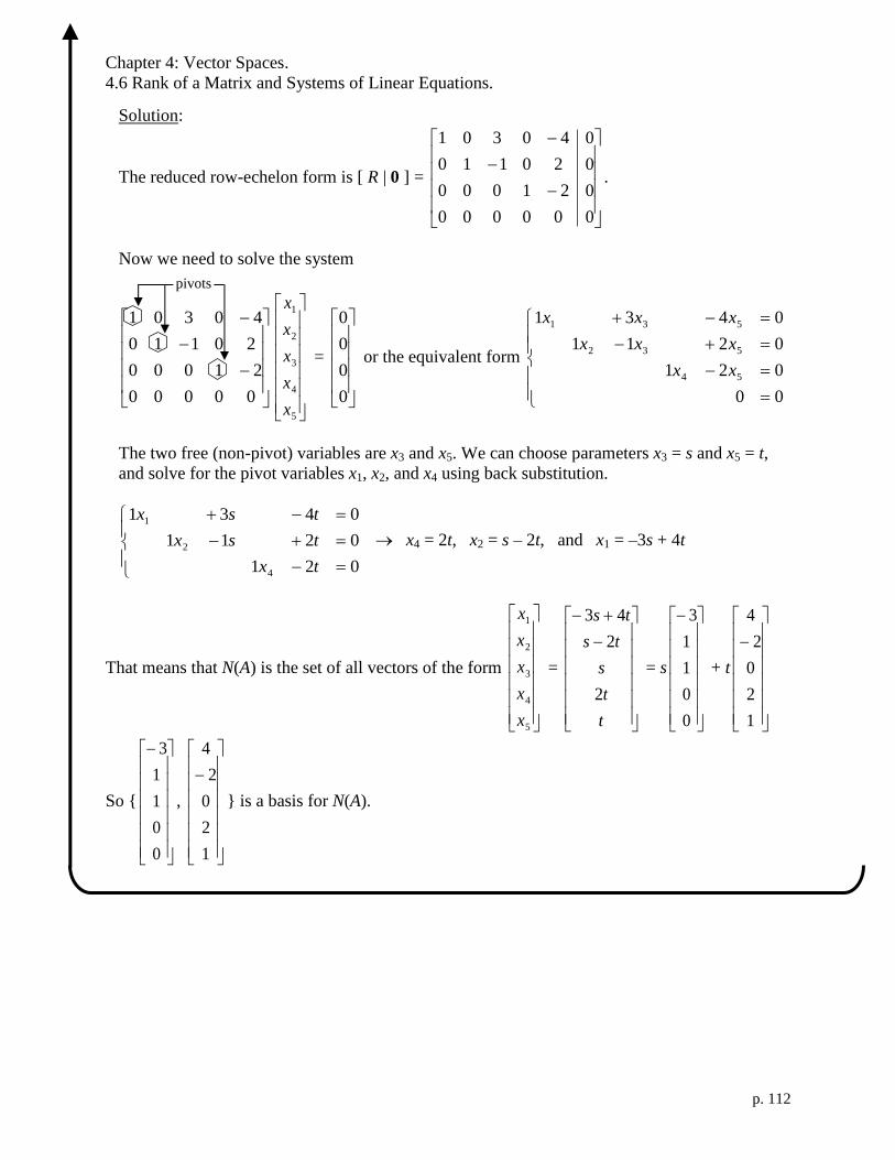
Chapter 4: Vector Spaces.
4.6 Rank of a Matrix and Systems of Linear Equations.
p. 112
Solution:
The reduced row-echelon form is [ R | 0 ] =
000000
021000
020110
040301
.
Now we need to solve the system
00000
21000
20110
40301
5
4
3
2
1
x
x
x
x
x
=
0
0
0
0
or the equivalent form
00
021
0211
0431
54
532
531
xx
xxx
xxx
The two free (non-pivot) variables are x3 and x5. We can choose parameters x3 = s and x5 = t,
and solve for the pivot variables x1, x2, and x4 using back substitution.
021
0211
0431
4
2
1
tx
tsx
tsx
x4 = 2t, x2 = s – 2t, and x1 = –3s + 4t
That means that N(A) is the set of all vectors of the form
5
4
3
2
1
x
x
x
x
x
=
t
t
s
ts
ts
2
2
43
= s
0
0
1
1
3
+ t
1
2
0
2
4
So {
0
0
1
1
3
,
1
2
0
2
4
} is a basis for N(A).
pivots

Chapter 4: Vector Spaces.
4.6 Rank of a Matrix and Systems of Linear Equations.
p. 113
S*
.(
Example: Find a basis for nullspace of
A =
2482
1110
1241
.
Solution:
Now that we have solved Ax = 0, let us consider Ax = b, where b 0. We have already seen (Ch.
1.2) that Ax = b has an infinite number of solutions if there are more variables than equations (n
> m). And since you can’t have more pivots than rows, m r, so n > r, or > 0.
Theorem 4.18 Solutions of a Nonhomogeneous System Ax = b
If xp is a particular solution to the nonhomogeneous equation Ax = b, then every solution of this
system can be written in the form x = xp + xh, where xh is a solution of the corresponding
homogeneous system Ax = 0, i.e. xh is in N(A). The general solution of Ax = b, parameterized by
the free parameters t1, t2, …, t is
x = xp + t1x1 + t2x2 + … + t x
Proof
Let x be any solution of Ax = b. Then (x – xp) is a solution of the homogeneous system Ax = 0,
because
A(x – xp) = Ax – Axp = b – b = 0
If we let xp = x – xp, then x = xp + xh.
(For ease of calculation, we usually find xp by solving Ax = b when all of the free variables are
set to zero.)
From Thm. 4.17+ we know that xh = t1x1 + t2x2 + … + tx.

Chapter 4: Vector Spaces.
4.6 Rank of a Matrix and Systems of Linear Equations.
p. 114
.(
Example: Find the general solution (the set of all solutions) of the system of linear system.
21521
145322
85533105
052
54321
54321
54321
54321
xxxxx
xxxxx
xxxxx
xxxxx
Solution:
2151121
1453221
85533105
051121
rref
000000
341000
260100
150021
To find xp, set the free variables x2 = 0, x5 = 0.
3)0(41
2)0(61
1)0(5)0(21
4
3
1
x
x
x
So x4 = –3, x3 = 2, x1 = 1. xp =
0
3
2
0
1
To find xh, set x2 = s, x5 = t. Ax = 0
041
061
0521
4
3
1
tx
tx
tsx
So x4 = –4t, x3 = –6t, x1 = –2s + 5t. xh =
t
t
t
s
ts
4
6
52
= s
0
0
0
1
2
+ t
1
4
6
0
5
x =
0
3
2
0
1
+ s
0
0
0
1
2
+ t
1
4
6
0
5

Chapter 4: Vector Spaces.
4.6 Rank of a Matrix and Systems of Linear Equations.
p. 115
Example: Find the general solution (the set of all solutions) of the system of linear system.
82
12143
293272
18103
zyx
zyx
zyx
zyx
Solution:
Example: Find the general solution (the set of all solutions) of the system of linear system.
822
29225
5426
19483
zyx
wzx
wzy
zyx
Solution:
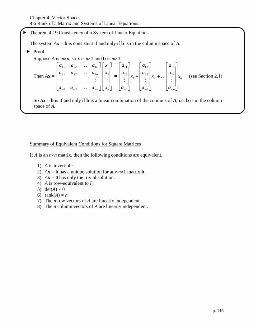
Chapter 4: Vector Spaces.
4.6 Rank of a Matrix and Systems of Linear Equations.
p. 116
S*
Theorem 4.19 Consistency of a System of Linear Equations
The system Ax = b is consistent if and only if b is in the column space of A.
Proof
Suppose A is mn, so x is n1 and b is m1.
Then Ax =
mnmm
n
n
aaa
aaa
aaa
21
22221
11211
nx
x
x
2
1
= n
mn
n
n
mm
x
a
a
a
x
a
a
a
x
a
a
a
2
1
2
2
22
12
1
1
21
11
(see Section 2.1)
So Ax = b is if and only if b is a linear combination of the columns of A, i.e. b is in the column
space of A.
Summary of Equivalent Conditions for Square Matrices
If A is an nn matrix, then the following conditions are equivalent.
1) A is invertible.
2) Ax = b has a unique solution for any n1 matrix b.
3) Ax = 0 has only the trivial solution.
4) A is row-equivalent to In.
5) det(A) 0
6) rank(A) = n
7) The n row vectors of A are linearly independent.
8) The n column vectors of A are linearly independent.
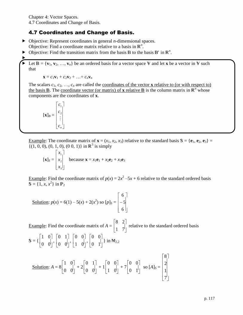
Chapter 4: Vector Spaces.
4.7 Coordinates and Change of Basis.
p. 117
S*
4.7 Coordinates and Change of Basis.
Objective: Represent coordinates in general n-dimensional spaces.
Objective: Find a coordinate matrix relative to a basis in Rn.
Objective: Find the transition matrix from the basis B to the basis B in Rn.
Let B = {v1, v2, …, vn} be an ordered basis for a vector space V and let x be a vector in V such
that
x = c1v1 + c2v2 + …+ cnvn
The scalars c1, c2, …, cn are called the coordinates of the vector x relative to (or with respect to)
the basis B. The coordinate vector (or matrix) of x relative B is the column matrix in Rn whose
components are the coordinates of x.
[x]B =
nc
c
c
2
1
Example: The coordinate matrix of x = (x1, x2, x3) relative to the standard basis S = {e1, e2, e3} =
{(1, 0, 0), (0, 1, 0), (0 0, 1)} in R3 is simply
[x]S =
3
2
1
x
x
x
because x = x1e1 + x2e2 + x3e3
Example: Find the coordinate matrix of p(x) = 2x2 –5x + 6 relative to the standard ordered basis
S = {1, x, x2} in P2
Solution: p(x) = 6(1) – 5(x) + 2(x2) so [p]S =
6
5
6
Example: Find the coordinate matrix of A =
71
28 relative to the standard ordered basis
S = {
00
01,
00
10,
01
00,
10
00} in M2,2
Solution: A = 8
00
01 + 2
00
10 + 1
01
00 + 7
10
00 so [A]S =
7
1
2
8

Chapter 4: Vector Spaces.
4.7 Coordinates and Change of Basis.
p. 118
Example 1: Given that the coordinate matrix of x in R2 relative to the nonstandard ordered basis
B = {v1, v2} = {(1, 0), (1, 2)} is
[x]B =
2
3
Find the coordinate matrix of x relative to the standard basis B = {u1, u2} = {(1, 0), (0, 1)} =
S.
Solution: [x]B =
2
3 means that x = 3v1 + 2v2 = 3(1, 0) + 2(1, 2) = (5, 4).
Now (5, 4) = 5(1, 0) + 4(0, 1) = 5u1 + 4u2 so [x]B=S =
4
5.
Another method is to take the coordinate matrices relative to B of
x = 3v1 + 2v2 =
21 vv
2
3 to obtain [x]B=S =
'2'1 ][][ BB vv
2
3 =
20
11
2
3 =
4
5.
This procedure is called a change of basis from B to B. Given [x]B, we found [x]B using an
equation of the form
[x]B = P1
[x]B where P–1
=
'2'1 ][][ BB vv .
The matrix P–1
is called the transition matrix from B to B.
Example 2: Given that the coordinate matrix of x in R3 relative to the standard ordered basis
B = S = {e1, e2, e3} is
[x]B =
1
2
1
.
Find the coordinate matrix of x relative to the nonstandard ordered basis B = {u1, u2, u3} =
{(1, 0, 1), (0, –1, 2), (2, 3, –5)}.

Chapter 4: Vector Spaces.
4.7 Coordinates and Change of Basis.
p. 119
S*
Solution: Write x as a linear combination of the vectors in B:
x = c1u1 + c2u2 + c3u3=
321 uuu
3
2
1
c
c
c
= [x]B =
BBB ][][][ 321 uuu
3
2
1
c
c
c
Since B = S,
1
2
1
=
521
310
201
3
2
1
c
c
c
so
3
2
1
c
c
c
=
1
521
310
201
1
2
1
=
2
8
5
.
Thus we have [x]B=S =
3
2
1
c
c
c
=
2
8
5
.
Moreover, we found that [x]B =
BBB ][][][ 321 uuu [x]B
Comparing to [x]B = P1
[x]B after Example 1above, we must have
[x]B = P[x]B where P =
BBB ][][][ 321 uuu .
The matrix P is called the transition matrix from B to B.
Given nonstandard bases B = {v1, v2, …, vn}, B = {u1, u2, …, un}, and the standard basis S =
{e1, e2, …, en} of Rn. Define matrices
BBS =
SnSS ][][][ 21 vvv and (B)BS =
SnSS ][][][ 21 uuu .
(B and B are square, invertible matrices.) B is the transition matrix from B to S; B is the
transition matrix from B to S. To get P–1
, the transition matrix from B to B, first apply BBS,
then apply (B)–1
SB.
P–1
= (B)–1
B or (P–1
)BB = (B)–1
SB BBS
The inverse is
P = B–1
B or PBB = (B–1
)SB (B)BS
Chapter 4: Vector Spaces.
4.7 Coordinates and Change of Basis.
p. 120
Example: Given B = {v1, v2, v3} = {(1, 0, 1), (1, 1, 0), (0, 1, 1)} and [x]B =
1
3
2
. Find [x]S
Solution:
Example: Given B = {u1, u2, u3} = {(8, 11, 0), (7, 0, 10), (1, 4, 6)} and x =(3, 19, 2). Find [x]B
Solution:
Example: Given B = {v1, v2, v3} = {(1, 0, 2), (0, 1, 3), (1, 1, 1)},
B = {u1, u2, u3} = {(2, 1, 1), (1, 0, 0), (0, 2, 1)}, and [x]B =
1
2
1
.
Find the transition matrix P from B to B the transition matrix P–1
from B to B, and [x]B.
Solution:

Chapter 5: Inner Product Spaces.
5.1 Length and Dot Product in Rn.
p. 121
S*
Chapter 5: Inner Product Spaces.
5.1 Length and Dot Product in Rn.
Objective: Find the length of a vector and find a unit vector.
Objective: Find the distance between two vectors.
Objective: Find a dot product and the angle between two vectors, determine orthogonality, and
verify the Cauchy-Schwarz Inequality, the triangle inequality, and the Pythagorean Theorem.
Objective: Use a matrix product to represent a dot product.
From the Pythagorean Theorem, we know that the length, or norm, of a vector v in R2 is
||v|| =2
2
2
1 vv . Also from the Pythagorean Theorem, in R3 we have
||v|| = 2
3
22
2
2
1 vvv
=
2
3
2
2
2
1 vvv .
In Rn we define the length or norm of v to be ||v|| =
22
2
2
1 nvvv
Notice that
|v|| 0
||v|| = 0 if and only if v = 0.
A unit vector is a vector whose length is one. In R2 and R3
alternate notation is sometimes used
for the standard unit vectors
i = (1, 0), j = (0, 1) in R2
i = (1, 0, 0), j = (0, 1, 0) , k = (0, 0, 1) in R3
Two nonzero vectors u and v are parallel when one of them is a scalar multiple of the other:
u = cv. If c > 0, then u and v have the same direction. If c < 0, then u and v have opposite
directions.
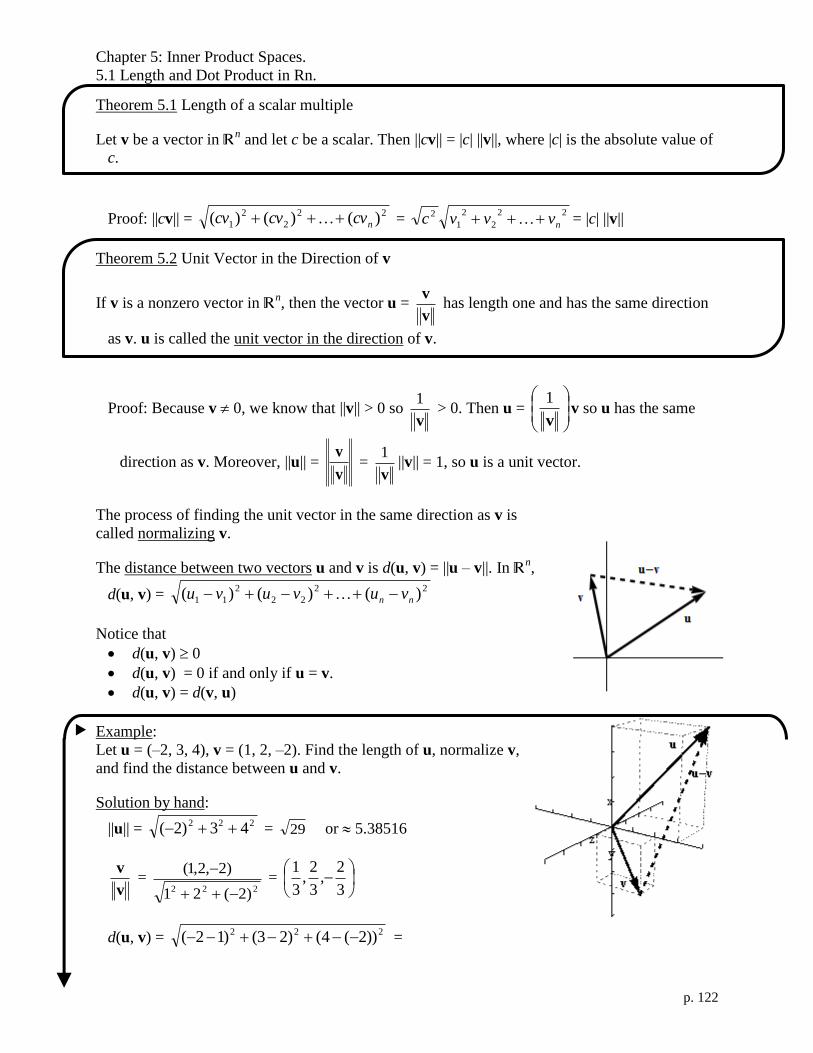
Chapter 5: Inner Product Spaces.
5.1 Length and Dot Product in Rn.
p. 122
Theorem 5.1 Length of a scalar multiple
Let v be a vector in Rn and let c be a scalar. Then ||cv|| = |c| ||v||, where |c| is the absolute value of
c.
Proof: ||cv|| = 22
2
2
1 )()()( ncvcvcv = 22
2
2
1
2
nvvvc = |c| ||v||
Theorem 5.2 Unit Vector in the Direction of v
If v is a nonzero vector in Rn, then the vector u =
v
v has length one and has the same direction
as v. u is called the unit vector in the direction of v.
Proof: Because v 0, we know that ||v|| > 0 so v
1 > 0. Then u =
v
1v so u has the same
direction as v. Moreover, ||u|| = v
v =
v
1||v|| = 1, so u is a unit vector.
The process of finding the unit vector in the same direction as v is
called normalizing v.
The distance between two vectors u and v is d(u, v) = ||u – v||. In Rn,
d(u, v) = 22
22
2
11 )()()( nn vuvuvu
Notice that
d(u, v) 0
d(u, v) = 0 if and only if u = v.
d(u, v) = d(v, u)
Example:
Let u = (–2, 3, 4), v = (1, 2, –2). Find the length of u, normalize v,
and find the distance between u and v.
Solution by hand:
||u|| = 222 43)2( = 29 or 5.38516
v
v =
222 )2(21
)2,2,1(
=
3
2,
3
2,
3
1
d(u, v) = 222 ))2(4()23()12( =

Chapter 5: Inner Product Spaces.
5.1 Length and Dot Product in Rn.
p. 123
S*
222 61)3( = 46 = 6.78233
Solution using Mathematica:
u={-2,3,4} Out = {-2,3,4}
Norm[u] Out =
v={1,2,-2} Out = {1,2,-2}
Normalize[v] Out =
Norm[u-v] Out =
Solution using TI-89: [-2,3,4]
U
[1,2,-2]V
MatrixNorms norm(U)
MatrixVector ops unitV(V)
MatrixNorms norm(U-
V)
To find the angle between to vectors in Rn, we start with the Law of
Cosines in R2.
||u – v||2 = ||u||
2 + ||v||
2 – 2||u|| ||v|| cos( )
(u1 – v1)2 + (u2 – v2)
2 = u1
2 + u2
2 + v1
2 + v2
2 – 2||u|| ||v|| cos( )
u12 –2u1v1 + v1
2 + u2
2 –2u2v2 + v2
2 = u1
2 + u2
2 + v1
2 + v2
2 – 2||u|| ||v|| cos( )
–2u1v1 –2u2v2 = – 2||u|| ||v|| cos( )
u1v1 + u2v2 = ||u|| ||v|| cos( )
This equation leads us to the following definitions.
The dot product between two vectors u = (u1, u2, …, un) and v = (v1, v2, …, vn) in Rn
u•v = u1v1 + u2v2 + … + unvn
The angle between two nonzero vectors u and v in Rn is =
vu
vuarccos , 0 .
u
v
u – v

Chapter 5: Inner Product Spaces.
5.1 Length and Dot Product in Rn.
p. 124
Two vectors u and v in Rn are orthogonal (perpendicular) when u•v = 0. (Notice that the 0 vector
is orthogonal to every vector.)
We often represent a vectors u = (u1, u2, …, un) and v = (v1, v2, …, vn) in Rn by their coordinate
matrices relative to the standard basis {e1, e2, …, en}
u =
nu
u
u
2
1
and v =
nv
v
v
2
1
We then write uTv for u•v because u
Tv = [u1v1 + u2v2 + … + unvn].
Warning: In our formulas, we will be sloppy and pretend that uTv is equal to the scalar u•v.
However, Mathematica and the TI-89 know that uTv is a 11 matrix, and will not let you use it
as a scalar.
Example: Using u = (–2, 3, 4), v = (1, 2, –2) from the previous
example, find u•v and the angle between u and v.
Solution by hand:
u•v = (–2)(1) + (3)(2) + (4)(–2) = –4
||u|| = 222 43)2( = 29 or 5.38516
||v|| = = 222 )2(21 = 3
=
293
4arccos 1.821 or 104.3
Solution using Mathematica:
u.v Out = 4
ArcCos[u.v/Norm[u]/Norm[v]] Out =
Out = 1.82099
Solution using TI-89:
MatrixVector ops
dotP(U,
V)
MatrixVector ops dotP(u, v)
MatrixNorms norm(u)
MatrixNorms norm(v))
MatrixVector ops dotP(u, v)
period, not
asterisk

Chapter 5: Inner Product Spaces.
5.1 Length and Dot Product in Rn.
p. 125
MatrixNorms norm(u)
MatrixNorms norm(v))
To obtain a decimal approximation instead of an exact formula, use N[...] in Mathematica or
instead of on the TI-89. You can change modes between degrees and radians on
the TI-89 using Angle……… DEGREE
Theorem 5.3 Properties of the Dot Product
If u, v, and w are vectors in Rn and c is a scalar, then
1) u•v = v•u
2) u•(v + w) = u•v + u•w
3) c(u•v) = (cu)•v = u•(cv)
4) v•v = ||v||2
5) v•v 0 and v•v = 0 if and only if v = 0.
Proof of 5.3.2:
u•(v + w) =
Rn combined with the usual operations of vector addition, scalar multiplication, vector length,
and the dot product is called Euclidean n-space.
(Optional aside: non-Euclidean spaces include elliptic space, which is curved, cannot be
smoothly mapped Rn and a has a different definition of distance; hyperbolic space, which is
curved and has different definition of distance; and Minkowski space, used in Einstein’s special
relativity, which replaces the non-negative dot product with an “interval” that can be negative.)
opti
onal
opti
on
al

Chapter 5: Inner Product Spaces.
5.1 Length and Dot Product in Rn.
p. 126
S*
S*
Theorem 5.4 The Cauchy-Schwarz Inequality
If u and v are vectors in Rn, then |u•v| ||u|| ||v||, where |u•v| is the absolute value of u•v.
Proof
If u = 0, then equality holds, because
|u•v| = |0•v| = |0| = 0, and ||u|| ||v|
= ||0|| ||v|| = 0 ||v|| = 0.
If u 0, then let t be any real number and consider the vector tu + v. Then
0 || tu + v ||2 =
The left-hand side is a quadratic function f (t) = at2 + bt + c, where
a = , b = , c =
The quadratic formula is 𝑡 =−𝑏±√𝑏2−4𝑎𝑐
2𝑎
Because f (t) 0, we have either one or zero roots, so 𝑏2 − 4𝑎𝑐 ≤ 0
Theorem 5.5 The Triangle Inequality
If u and v are vectors in Rn, then ||u + v|| ||u|| + ||v||.
Proof
||u + v||2 =

Chapter 5: Inner Product Spaces.
5.1 Length and Dot Product in Rn.
p. 127
S*
Theorem 5.6 The Pythagorean Theorem
If u and v are vectors in Rn, then u and v are orthogonal if and only if ||u + v||
2 = ||u||
2 + ||v||
2.
Proof
By definition, u and v are orthogonal if and only if
||u + v||2 =
The conclusion follows from these two equations.

Chapter 5: Inner Product Spaces.
5.2 Inner Product Spaces.
p. 129
*
5.2 Inner Product Spaces.
Objective: Determine whether a function defines an inner product.
Objective: Find the inner product of two vectors in Rn, Mm,n, Pn, and C[a,b].
Objective: Use the inner product to find angles between two vectors and determine whether two
vectors are orthogonal.
Objective: Find an orthogonal projection of a vector onto another vector in an inner product
space.
The inner product is an extension of the concept of the dot product from Rn to a general vector
space. The standard dot product, also called the Euclidean inner product, on Rn is written as u•v,
while the general inner product on a vector space V is written as u, v.
Definition of Inner Product
Let u, v, and w be vectors in a vector space V, and let c be any scalar. An inner product on V is a
function that associates a real number u, v with each pair of vectors u and v. and satisfies the
following axioms.
1) u, v = v, u Symmetric
2) u, v + w = u, v + u, w
3) cu, v = cu, v
4) v, v 0 and v, v = 0 if and only if v = 0. Nonnegative
A vector space V with an inner product is called an inner product space.
Example: Consider R2. Let u =
2
1
u
u and v =
2
1
v
v. Instead of the Euclidean inner product
uTv, let u, v = u
T
31
12v = 2u1v1 – u1v2 – u2v1 + 3u2v2. Show that u, v is an inner
product.
Solution:
1) v, u = vT
31
12u = 2v1u1 – v1u2 – v2u1 + 3v2u2 = u, v
2) Let A =
31
12. We know that for matrix multiplication, u, v + w = u
TA(v + w) =
(uTA)(v + w) = (u
TA)v + (u
TA)w = u
TAv + u
TAw = u, v + u, w.
3) We know that for matrix multiplication, cu, v = c(uT
31
12v) = (cu
T)
31
12v =
= cu, v.

Chapter 5: Inner Product Spaces.
5.2 Inner Product Spaces.
p. 130
4) v, v = 2v12 – 2v1v2 + 3v2
2 = v1
2 + 2v2
2 + v1
2 – 2v1v2 + v2
2 = v1
2 + 2v2
2 + (v1 – v2)
2 0,
and v, v = if and only if v1 = 0, v2 = 0, and v1 – v2 = 0 if and only if v = 0.
Example: Consider R4. Let u =
z
y
x
t
u
u
u
u
and v =
z
y
x
t
v
v
v
v
. Instead of the Euclidean inner product
uTv, let u, v = u
T
1000
0100
0010
0002c
v, where c is a positive constant (the speed of light), so
u, v = –c2utvt + uxvx + uyvy + uzvz. Show that u, v is not an inner product. (Optional aside: u,
v is called the spacetime interval.)
Solution:
4) v, v = –c2vt
2 + vx
2 + vy
2 + vz
2 which can be less than zero, for example when v =
0
0
0
1
.
Note: Axioms 2 and 3 are satisfied because of the rules of matrix multiplication. Axiom 1 is
satisfied because the matrix is symmetric (AT = A).
Theorem 5.7 Properties of Inner Products
If u, v, and w are vectors in an inner product space V “over the real numbers” and c is a scalar,
then
1) 0, v = v, 0 = 0
2) u + v, w = u, w + v, w
3) u, cv = cu, v
Proof of 5.7.1: 0, v = 0v, v = 0v, v = 0. By the symmetric property, v, 0 = 0, v = 0
Proof of 5.7.2: u + v, w = w, u + v Symmetry
= w, u + w, v Axiom 2
= u, w + v, w Symmetry
Proof of 5.7.3: u, cv = cv, u Symmetry
= cv, u Axiom 3
= cu, v Symmetry
opti
onal

Chapter 5: Inner Product Spaces.
5.2 Inner Product Spaces.
p. 131
*
Together with the inner product axioms, Thm 5.7 says that the inner product is linear in each of
its arguments (we will study linear operators much more in Chapter 6.) Linearity is
essentially the same as distributivity:
Dot product: (2u + 3v)•(5x + 7y) = 10(u•x) + 14(u•y) + 15(v•x) + 21(v•y)
General inner product: 2u + 3v, 5x + 7y = 10u, x + 14u, y + 15v, x + 21v, y
Let u and v be vectors in an inner product space V.
The length, or norm, of u is ||u|| = uu, .
The distance between two vectors u and v is d(u, v) = ||u – v||.
The angle between two nonzero vectors u and v is given by =
vu
vu,arccos , 0 .
Two vectors u and v in Rn are orthogonal (perpendicular) when u, v = 0. (Notice that the 0
vector is orthogonal to every vector.)
If ||u|| = 1 then u is called a unit vector. If v is any nonzero vector, then u = v
v is the unit vector
in the direction of v. Notice that the definition of angle presumes that –1 vu
vu, 1. This is
guaranteed by the Cauchy-Schwarz Inequality (Theorem 5.8.1).
Properties of Length
1) ||u|| 0
2) ||u|| = 0 if and only if u = 0.
3) ||cu|| = |c| ||u||
These follow from the axioms in the definition of inner product and the definition of norm.
Properties of Distance
1) d(u, v) 0
2) d(u, v) = 0 if and only if u = v.
3) d(u, v) = d(v, u)
These follow from the axioms in the definition of inner product and the definition of distance.

Chapter 5: Inner Product Spaces.
5.2 Inner Product Spaces.
p. 132
.(
Example: Let A =
2221
1211
aa
aa and B =
2221
1211
bb
bb be two matrices in M2,2 and define the inner
product A, B = a11b11 + a12b12 + a21b21 + a22b22.
Let I =
10
01, R =
01
10 and L =
45
43
43
45
.
a) Find the norm of I =
10
01.
Solution:
b) Find the inner product of and angle between R and L. Are they orthogonal?
Solution:
c) Find the inner product of and angle between I and L. Are they orthogonal?
Solution:

Chapter 5: Inner Product Spaces.
5.2 Inner Product Spaces.
p. 133
.(
Example: Let p and q be two polynomials in P and define the inner product
p, q =
1
1
)()( dxxqxp
a) Find the norm of p(x) = 1. (Sometimes we will just say “Find the norm of 1.”)
Solution:
b) Find the inner product of p(x) = 1 and q(x) = x. Are they orthogonal?
Solution:
c) Find the angle between 1 and x2. Are they orthogonal?
Solution:
Theorem 5.8
Let u and v be vectors in an inner product space V.
1) Cauchy-Schwarz Inequality: | u, v | ||u|| ||v||
2) Triangle inequality: ||u + v|| ||u|| + ||v||
3) Pythagorean Theorem: u and v are orthogonal if and only if ||u + v||2 = ||u||
2 + ||v||
2.
The proofs are the same as the proofs of Theorems 5.4, 5.5, and 5.6, except that we replace u•v
with u, v. A result such as the triangle inequality, which seems intuitive in R2 and R3
, can be
generalized through linear algebra to some less obvious statements about functions in
C[a, b].

Chapter 5: Inner Product Spaces.
5.2 Inner Product Spaces.
p. 134
Example: Consider f (x) = cos(x) and g(x) = 2
4
(/2 – x)(/2 + x) in C[–/2, /2] with the inner
product f , g =
2/
2/
)()(
dxxgxf . Verify the triangle inequality by direct calculation.
Solution: The triangle inequality is || f + g || || f || + || g ||.
|| f ||2 =
|| g ||2 =
|| f + g ||2 =
|| f + g || =
|| f || + || g || =
Orthogonal Projections: Let u and v be two vectors in R2. If v is nonzero,
then u can be orthogonally projected onto v. This projection is denoted by
projv u. Because projv u is a scalar multiple of v, we can write
projv u = av
v
(Recall that v
v is the unit vector in the direction of v.)
Then a = ||u|| cos = ||u|| vu
vu =
v
vu
projv u = vv
vu2
= v
vv
vu
projv u v
u

Chapter 5: Inner Product Spaces.
5.2 Inner Product Spaces.
p. 135
*
.(
Let u and v be vectors in a general inner product space V. The orthogonal projection of u onto v
is
proj𝐯 𝐮 = ⟨𝐮, 𝐯⟩
⟨𝐯, 𝐯⟩ 𝐯
Example: Use the Euclidean inner product find the orthogonal projection of u = (1, 0, 0) onto
v = (1, 1, 1) and of v onto u .
Solution:
projv u =
projv u =

Chapter 5: Inner Product Spaces.
5.2 Inner Product Spaces.
p. 136
.(
Theorem 5.9 Orthogonal Projection and Distance
Let u and v be two vectors in an inner product
space V such that v 0. Then
d(u, projv u) < d(u, cv) whenever c vv
vu
,
,
That is to say, the orthogonal projection projv u is the vector parallel to v that is closest to u.
Proof: Let b = vv
vu
,
,, c
vv
vu
,
,, p = cv – bv, q = u – bv, and t = u – cv.
The p is orthogonal to q, because
p, q = cv – bv, u – bv
= cv, u – cbv, v – bv, u + b2v, v
= cu, v – cvv
vu
,
,v, v –
vv
vu
,
,u, v +
2
2
,
,
vv
vuv, v
= cv, u – cv, u – vv
vu
,
,2
+ vv
vu
,
,2
= 0.
So the Pythagorean Theorem tells us ||t||2 = ||p||
2 + ||q||
2 > ||q||
2 because p 0 because c b.
Therefore, d(u, projv u) = ||q|| < ||t|| = d(u, cv).
Example: Consider C[–, ] with the inner product f , g =
dxxgxf )()( .
Find the projection of f (x) = x onto g(x) = sin(x).
Solution:
projg f = )(,
,xg
gg
gf.
cv v
u
d(u, cv)
projv u v
u
d(u, projv u)
u
t = u – cv q
bv
p = (c – b)v
Chapter 5: Inner Product Spaces.
5.3 Orthogonal Bases: Gram-Schmidt Process.
p. 137
S*
S*
5.3 Orthogonal Bases: Gram-Schmidt Process.
Objective: Show that a set of vectors is orthogonal and forms an orthonormal basis.
Objective: Represent a vector relative to an orthonormal basis.
Objective: Apply the Gram-Schmidt orthonormalization process.
Although a vector space can have many different bases, some bases may be easier to work with
than others. For example, in R3, we often use the standard basis S = {e1, e2, e3} = {(1, 0, 0),
(0, 1, 0), (0 0, 1)}. Two properties that make the standard basis desirable are that
1) The vectors are normalized, i.e. each basis vector is a unit vector: ||ei|| = 1 for i = 1, 2, 3.
2) The vectors are mutually orthogonal: ei•ej = 0 whenever i j, i.e.
e1•e2 = 0,
e1•e3 = 0,
e2•e3 = 0
A set S of vectors in an inner product space V, is called orthogonal when every pair of vectors in
S is orthogonal. If, in addition, each vector in the set is a unit vector, then S is called
orthonormal.
If S = {v1, v2, …, vn} then these definitions can be written as
S is orthogonal if and only if vi•vj = 0 whenever i j.
S is orthonormal if and only if vi•vj = 0 whenever i j, and ||ei|| = 1 for i = 1, 2, …, n.
Example: Show that S = {(cos, sin, 0)}, (–sin, cos, 0), (0, 0, 1)} is an orthonormal set.
Solution: S is orthogonal, because
(cos, sin, 0) • (–sin, cos, 0) = – cos sin + sin cos = 0
(cos, sin, 0) • (0, 0, 1) = 0
and (–sin, cos, 0) • (0, 0, 1) = 0
S is normalized, because
||(cos, sin, 0)|| = 222 0sincos = 1
||(–sin, cos, 0)|| = 222 0cossin = 1

Chapter 5: Inner Product Spaces.
5.3 Orthogonal Bases: Gram-Schmidt Process.
p. 138
||(0, 0, 1)|| = 222 100 = 1
Theorem 5.10 Orthogonal Sets are Linearly Independent
If S = {v1, v2, …, vn} is an orthogonal set of nonzero vectors in an inner product space V, then S
is linearly independent.
Proof: suppose c1v1 + c2v2 + …+ cnvn = 0
Then (c1v1 + c2v2 + …+ cnvn), vi = 0, vi for each of the vi
We can distribute the inner product on the left-hand side to obtain
Because S is orthogonal, when j i,
so equation becomes
Because vi 0,
Example: Consider C[0, 2] with the inner product f , g = 2
0
)()( dxxgxf .
Show that the set {1, cos(x), sin(x), cos(2x), sin(2x), …, cos(nx), sin(nx)} is a linearly
independent orthogonal set.
Solution: We use software to integrate the following expressions, and we use these identities to
evaluate the results:
1)2cos(
0)2sin(
k
k
whenever k is an integer
1, sin(nx) = 2
0
)sin(1 dxnx =
2
0
)cos(
n
nx =
nn
11 = 0
1, cos(nx) = 2
0
)cos(1 dxnx =
2
0
)sin(
n
nx = 0 – 0 = 0

Chapter 5: Inner Product Spaces.
5.3 Orthogonal Bases: Gram-Schmidt Process.
p. 139
S*
S*
sin(mx), sin(nx) when m n is
2
0
)sin()sin( dxnxmx =
2
0)(2
))sin((
)(2
))sin((
nm
xnm
nm
xnm = (0 – 0) – (0 – 0) = 0
cos(mx), cos(nx) when m n is
2
0
)cos()cos( dxnxmx =
2
0)(2
))sin((
)(2
))sin((
nm
xnm
nm
xnm = (0 + 0) – (0 + 0) = 0
cos(mx), sin(nx) when m n is
2
0
)sin()cos( dxnxmx =
2
0)(2
))cos((
)(2
))cos((
nm
xnm
nm
xnm =
)(2
1
)(2
1
)(2
1
)(2
1
nmnmnmnm = 0
cos(nx), sin(nx) = 2
0
)sin()cos( dxnxnx =
2
0
2
2
)(cos
n
nx =
nn 2
1
2
1 = 0
Corollary Orthogonal Bases
If V is an inner product space of dimension n, then any orthogonal set of n nonzero vectors in V
is a basis for V.
Example: Show that S = {(0, 1, 0, 1), (–1, –1, 2, 1), (2, –1, 0, 1), (2, 2, 3, –2)} is an orthogonal
basis of R4.
Solution: S is orthogonal, because
(0, 1, 0, 1)•(–1, –1, 2, 1) = 0 – 1 + 0 + 1 = 0
(0, 1, 0, 1)•(2, –1, 0, 1) = 0 –1 + 0 – 1 = 0
(0, 1, 0, 1)•(2, 2, 3, –2) = 0 + 2 + 0 – 2 = 0
(–1, –1, 2, 1)•(2, –1, 0, 1) = –2 + 1 + 0 + 1 = 0
(–1, –1, 2, 1)•(2, 2, 3, –2) = –2 – 2 + 3 – 2 = 0
and (2, –1, 0, 1)•(2, 2, 3, –2) = 4 – 2+ 0 – 2 = 0
By the Corollary to Theorem 5.10, S is an orthogonal basis for R4.

Chapter 5: Inner Product Spaces.
5.3 Orthogonal Bases: Gram-Schmidt Process.
p. 140
S*
Theorem 5.11 Coordinates Relative to an Orthonormal Basis
If B = {v1, v2, …, vn} is an orthonormal basis for an inner product space V, then the coordinate
representation of a vector w relative to B is
w = w, v1v1 + w, v2 v2 + … +w, vn vn
Proof: Because B is a basis for V, there are unique scalars c1, c2, …, cn such that
w = c1v1 + c2v2 + …+ cnvn
Taking the inner product with vi of both sides of the equation gives
w, vi = (c1v1 + c2v2 + …+ cnvn), vi
We can distribute the inner product on the left-hand side to obtain
Because S is orthonormal, when
so equation becomes
so
The coordinates of w relative to an orthonormal basis B are called the Fourier coefficients of w
relative to B. The corresponding coordinate matrix is
[w]B =
nc
c
c
2
1
=
nvw
vw
vw
,
,
,
2
1
Note: contrast Thm 5.11 with [w]B =
1
21 ][][][
SnSS vvv [w]S
from Section 4.7 for a general, non-orthonormal basis B.

Chapter 5: Inner Product Spaces.
5.3 Orthogonal Bases: Gram-Schmidt Process.
p. 141
S*
S*
Example: Find the coordinate matrix of w = (–2, 6, 5) relative to the orthonormal basis
B = {(2
1,
2
1, 0), (–
6
2,
6
2,
3
22), (
3
2, –
3
2,
3
1)} of R3
.
Solution:
so the coordinate matrix is
Given any basis for a vector space, we can construct an orthonormal basis using a procedure
called the Gram-Schmidt Orthonormalization.
Theorem 5.12(Alt) (Alternative) Gram-Schmidt Orthonormalization Process
Let B = {v1, v2, …, vn} be a basis for an inner product space V.
Let B = {u1, u2, …, un}, where ui is given by
w1 = v1, ...........................................................................................................u1 = 1
1
w
w
w2 = v2 – v2, u1u1, ........................................................................................u2 = 2
2
w
w
w3 = v3 –v3, u1u1 – v3, u2u2,......................................................................u3 = 3
3
w
w
…
wn = vn – vn, u1u1 – vn, u2u2 – … – vn, u n–1un–1, ...................................un = n
n
w
w
Then B is an orthonormal basis for V. Moreover, span{ u1, u2, …, uk} = span{ v1, v2, …, vk} for
k = 1, 2, …, n.
Proof: First, B is normalized, since all of the ui are unit
vectors: ||ui||= 1. Second, observe that the terms of the form
vj, uiui are projections onto ui: vj, uiui = jivuproj
When we subtract jivuproj from vj, the resultant vector is
orthogonal to ui

Chapter 5: Inner Product Spaces.
5.3 Orthogonal Bases: Gram-Schmidt Process.
p. 142
S*
Now we prove by induction that B is also an orthonormal set.
If n =1, then there are no pairs of vectors in B, so there is nothing to prove.
If {u1, u2, …, uk–1} is an orthonormal set, then consider uk = k
k
w
w where
wk = vk – vk, u1u1 – vk, u2u2 – … – vk, ujuj – … – vk, uk–1uk–1.
Let j = 1, 2, …, k – 1. Then
uk, uj = nw
1(vk – vk, u1u1 – vk, u2u2 – … – vk, ujuj – … vk, uk–1uk–1), uj
=nw
1 (vk, uj – vk, u1u1, uj – vk, u2u2, uj – … – vk, ujuj, uj – …
– vk, uk–1uk–1, uj)
=nw
1 (vk, uj – vk, u1(0) – vk, u2(0) – … – vk, uj(1) – … – vk, uk–1(0))
=nw
1 (vk, uj – vk, uj) = 0
So {u1, u2, …, uk} is also an orthonormal set. By mathematical induction, B is orthonormal, and
since it has n vectors in an n-dimensional space, B is an orthonormal basis.
Example: Use the Gram-Schmidt orthonormalization process to construct an orthonormal basis
from B = {(1, 2, 2), (–1, –1,0), (1, 0, 0)}.
Solution:
w1 = (1, 2, 2) u1 = )2,2,1(
)2,2,1( = (
31 ,
32 ,
32 )
w2 = (–1, –1,0) – ((–1, –1,0)•(31 ,
32 ,
32 ))(
31 ,
32 ,
32 )
= (–1, –1,0) – (–1)(1, 2, 2)
= (–32 , –
31 ,
32 ) u2 =
),,(
),,(
32
31
32
32
31
32
= (–
32 , –
31 ,
32 )
w3 =
u3 =

Chapter 5: Inner Product Spaces.
5.3 Orthogonal Bases: Gram-Schmidt Process.
p. 143
Example: Use the Gram-Schmidt orthonormalization process to construct an orthonormal basis
from B = {1, x, x2} in P2 with the inner product p(x), q(x) =
1
1
)()( dxxqxp .
Solution: Let v1 = 1, v2 = x, and v3 = x2.
w1 = 1
u1 = 1
1
||1||2 =
1
1
11 dx = 1
1x = 2
u1 = 2
1
w2 =
u2 =


Chapter 5: Inner Product Spaces.
5.4 Mathematical Models and Least Squares Analysis (Optional).
p. 145
5.4 Mathematical Models and Least Squares Analysis (Optional).
Objective: Find the orthogonal complement of a subspace.
Objective: Solve a least squares problem.
In this section, we consider inconsistent systems of linear equations, and we find the “best
approximation” to a solution.
Example: Given a table of data. We want to find the
coefficients c0 and c1 of the line y = c0 + c1t
that “best fits” these points.
Solution: The system of linear equations that we
have to solve comes from plugging the three points
(ti, yi) into the equation c0 + c1ti = yi
33
12
01
10
10
10
cc
cc
cc
or
3
1
0
31
21
11
1
0
c
c. Let A =
31
21
11
, b =
3
1
0
, and x =
1
0
c
c
The system is inconsistent: reduced row-echelon form is
100
010
001
. (We also knew that there
would be no solution because the three points in the graph are not collinear.) But what is the
“best approximation”?
Recall that Ax = 10
3
2
1
1
1
1
cc
is always in the column space of A. But since Ax = b has no
solution, b is not in the column space of A. We want to find an x that gives the Ax that is
closest to b.
Least Squares Problem: Given an mn
matrix A and a vector b in Rm, find x in
Rn, such that ||Ax – b||
2 is minimized.
This gives the Ax that is closest to b. It is
customary to minimize ||Ax – b||2 instead
of ||Ax – b|| because ||Ax – b|| involves a
square root. Intuitively, we see that
Ax – b is orthogonal to the column space
of A.
t y
1 0
2 1
3 3
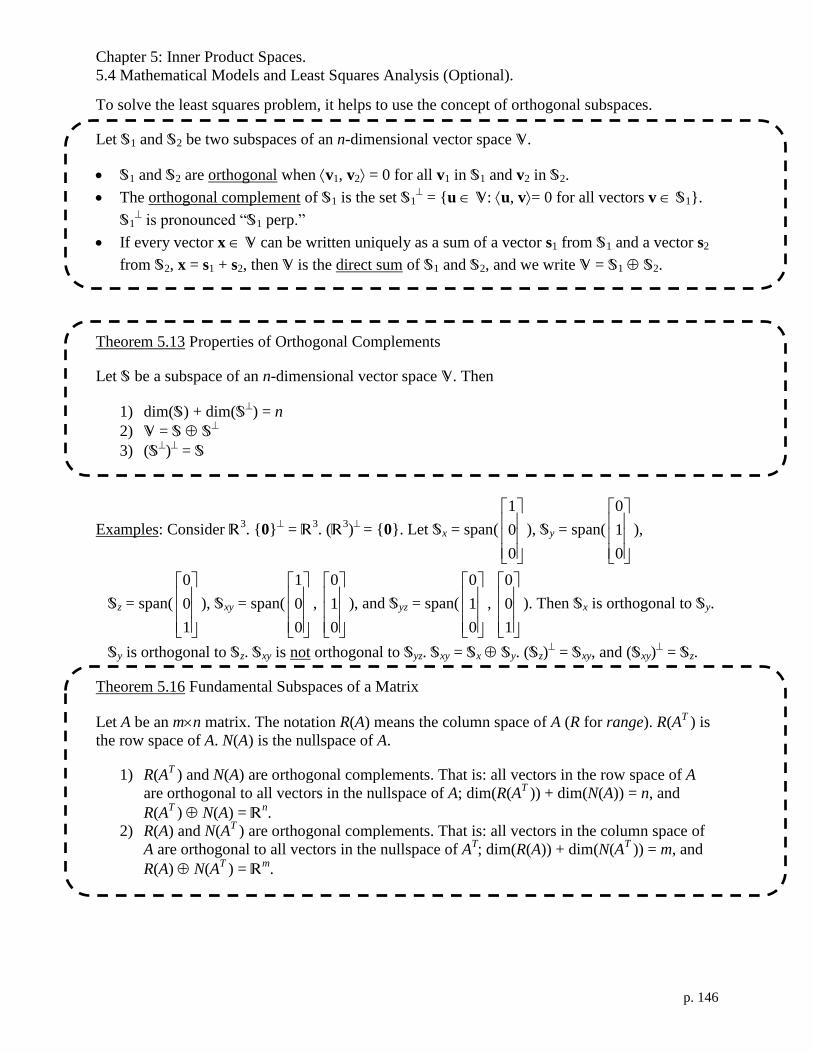
Chapter 5: Inner Product Spaces.
5.4 Mathematical Models and Least Squares Analysis (Optional).
p. 146
To solve the least squares problem, it helps to use the concept of orthogonal subspaces.
Let S1 and S2 be two subspaces of an n-dimensional vector space V.
S1 and S2 are orthogonal when v1, v2 = 0 for all v1 in S1 and v2 in S2.
The orthogonal complement of S1 is the set S1 = {u V: u, v= 0 for all vectors v S1}.
S1 is pronounced “S1 perp.”
If every vector x V can be written uniquely as a sum of a vector s1 from S1 and a vector s2
from S2, x = s1 + s2, then V is the direct sum of S1 and S2, and we write V = S1 S2.
Theorem 5.13 Properties of Orthogonal Complements
Let S be a subspace of an n-dimensional vector space V. Then
1) dim(S) + dim(S) = n
2) V = S S
3) (S) = S
Examples: Consider R3. {0}
= R3
. (R3)
= {0}. Let Sx = span(
0
0
1
), Sy = span(
0
1
0
),
Sz = span(
1
0
0
), Sxy = span(
0
0
1
,
0
1
0
), and Syz = span(
0
1
0
,
1
0
0
). Then Sx is orthogonal to Sy.
Sy is orthogonal to Sz. Sxy is not orthogonal to Syz. Sxy = Sx Sy. (Sz) = Sxy, and (Sxy)
= Sz.
Theorem 5.16 Fundamental Subspaces of a Matrix
Let A be an mn matrix. The notation R(A) means the column space of A (R for range). R(AT
) is
the row space of A. N(A) is the nullspace of A.
1) R(AT
) and N(A) are orthogonal complements. That is: all vectors in the row space of A
are orthogonal to all vectors in the nullspace of A; dim(R(AT
)) + dim(N(A)) = n, and
R(AT
) N(A) = Rn.
2) R(A) and N(AT
) are orthogonal complements. That is: all vectors in the column space of
A are orthogonal to all vectors in the nullspace of AT; dim(R(A)) + dim(N(A
T )) = m, and
R(A) N(AT
) = Rm.

Chapter 5: Inner Product Spaces.
5.4 Mathematical Models and Least Squares Analysis (Optional).
p. 147
Sketch of the proof:
1) N(A) ={x Rn: Ax = 0} shows that the nullspace is orthogonal to the row space, because the
null vector x is orthogonal to each row of A.
Ax = 0 is equivalent to
0) of row(
0) of 2 row(
0) of 1 row(
x
x
x
Am
A
A
dim(R(AT
)) + dim(N(A)) = n is rank + nullity = n, which we already know.
The basis vectors of R(AT
)) are linear independent of the basis of N(A) because they are
orthogonal to the basis of N(A), so the union of a basis of R(AT
)) and a basis of N(A) is a basis
of Rn, so R(A
T ) N(A) = Rn
.
2) Replace A with AT in Part (1), and use (A
T )T = A. When we replace A with A
T, we must
interchange m and n.
Example: Find the orthogonal complement of S = span(
0
0
2
1
,
1
0
1
0
).
Solution: S is the column space R(A), where A =
10
00
12
01
, so S = N(A
T).
To find N(A), solve Ax = 0
01010
00021rref
01010
02001
so 1x1 + 0x2 + 0s – 2t = 0
and 0x1 + 1x2 + 0s + 1t = 0
so x2 = –t and x1 = 2t
x =
t
s
t
t2
= s
0
1
0
0
+ t
1
0
1
2
so S = N(A
T) = span(
0
1
0
0
,
1
0
1
2
)
If S is a subspace of an n-dimensional vector space V and v is a vector in V, then v can be
written uniquely as the sum of a vector from S and a vector from S
v = s1 + s2, where s1 S and s2 S
because V = S S. Then s1 S is the orthogonal projection of v onto S, written vSproj

Chapter 5: Inner Product Spaces.
5.4 Mathematical Models and Least Squares Analysis (Optional).
p. 148
Theorem: v – vSproj is orthogonal to every vector in S.
Proof: v can be written uniquely as v = vSproj + s2, where s2 = v – vSproj S. Since
v – vSproj S, v – vSproj is orthogonal to every vector in S.
Theorem 5.15 Orthogonal Projection and Distance
Let S be a subspace of an n-dimensional vector space V and v be a vector in V. Then for all u
S, u vSproj , ||v – vSproj || < ||v – u||.
In other words, vSproj is the vector in S that is closest to v.
Proof: Let all u S, u vSproj so
v – u = (v – vSproj ) + ( vSproj – u)
Now v – vSproj is orthogonal to ( vSproj – u), so
by the Pythagorean Theorem,
||v – u||2 = ||v – vSproj ||
2 + || vSproj – u||
2
where || vSproj – u|| > 0 because u vSproj .
Therefore, ||v – u||2 > ||v – vSproj ||
2
||v – u|| > ||v – vSproj ||
To solve the least squares problem, we
need Ax – b (R(A)) = N(A
T ), so
AT(Ax – b) = 0, or
ATAx = A
Tb “Normal equations”
Solution to Least Squares Problem
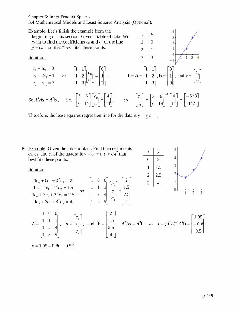
Chapter 5: Inner Product Spaces.
5.4 Mathematical Models and Least Squares Analysis (Optional).
p. 149
Example: Let’s finish the example from the
beginning of this section. Given a table of data. We
want to find the coefficients c0 and c1 of the line
y = c0 + c1t that “best fits” these points.
Solution:
33
12
01
10
10
10
cc
cc
cc
or
3
1
0
31
21
11
1
0
c
c. Let A =
31
21
11
, b =
3
1
0
, and x =
1
0
c
c
So ATAx = A
Tb , i.e.
146
63
1
0
c
c=
11
4, so
1
0
c
c =
1
146
63
11
4 =
2/3
3/5.
Therefore, the least-squares regression line for the data is y = 23 t –
35
Example: Given the table of data. Find the coefficients
c0, c1, and c2 of the quadratic y = c0 + c1t + c2t2 that
best fits these points.
Solution:
4331
5.2221
5.1111
2001
2
2
10
2
2
10
2
2
10
2
2
10
ccc
ccc
ccc
ccc
so
931
421
111
001
2
1
0
c
c
c
=
4
5.2
5.1
2
A =
931
421
111
001
, x =
2
1
0
c
c
c
, and b =
4
5.2
5.1
2
. ATAx = A
Tb so x = (A
TA)
–1A
Tb =
5.0
8.0
95.1
y = 1.95 – 0.8t + 0.5t2
t y
1 0
2 1
3 3
t y
0 2
1 1.5
2 2.5
3 4


Chapter 5: Inner Product Spaces.
5.5 Applications of Inner Product Spaces (Optional).
p. 151
5.5 Applications of Inner Product Spaces (Optional).
Objective: Find the nth
-order Fourier approximation of a function.
Objective: Given a subspace with an orthogonal or orthonormal basis, find the projection of a
vector onto that subspace.
Objective: Find the cross product of two vectors in R3.
Recall from Thm. 5.15 that vSproj is the unique vector in S that is closest to v.
Theorems 5.14 & 5.19 Projection onto a Subspace & Least Squares Approximation
If {u1, u2, …, un} is an orthonormal basis for a subspace S of a vector space V, and v V, then
vSproj = v, u1u1 + v, u2u2 + … + v, unun
If V is a space of functions, e.g. V = C[a, b] (so the ui are functions), then
fSproj = f, u1u1 + f, u2u2 + … + f, unun
is the least-squares approximating function of f with respect to S.
Proof: we will show that vSproj = v, u1u1 + v, u2u2 + … + v, unun by showing that v can be
written uniquely as the sum of a vector from S and a vector from S
v = s1 + s2, where s1 S and s2 S. Then by definition, vSproj = s1.
Let s1 = v, u1u1 + v, u2u2 + … v, unun
and s2 = v – v, u1u1 – v, u2u2 – … – v, unun
Then s1 S because it is a linear combination of vectors in S.
For each basis vector ui of S
ui, s2 = ui, (v – v, u1u1 – v, u2u2 – … – v, uiui – … – v, unun)
= ui, v – v, u1ui, u1 – v, u2ui, u2 – … – v, uiui, ui – … – v, unui, un
= ui, v – 0 – 0 – … – v, ui (1) – … – 0
= 0
Since all vectors in S are linear combinations of the {ui}, s2 is orthogonal to all vectors in S,
so s2 S.
Example: we know from 5.3 that set {1, cos(x), sin(x), cos(2x), sin(2x), …, cos(nx), sin(nx)} is a
an orthogonal set using the inner product f , g = 2
0
)()( dxxgxf . Let’s normalize the set.

Chapter 5: Inner Product Spaces.
5.5 Applications of Inner Product Spaces (Optional).
p. 152
||1||2 =
2
0
)1)(1( dx = 2.
For n 0, ||cos(nx)||2 =
2
0
)cos()cos( dxnxnx =
2
02
)cos()sin(
2
xn
nxnxx =
and ||sin(nx)||2 =
2
0
)sin()sin( dxnxnx =
2
02
)cos()sin(
2
xn
nxnxx =
So {2
1 ,
1 cos(x),
1 sin(x),
1 cos(2x),
1 sin(2x), …,
1 cos(nx),
1 sin(nx)} is an
orthonormal set.
The nth
-order Fourier approximation of a function f on the interval [0, 2] is the projection of f
onto span {2
1 ,
1 cos(x),
1 sin(x),
1 cos(2x),
1 sin(2x), …,
1 cos(nx),
1 sin(nx)}.
Fourier approximations are useful in modeling periodic functions such as sound waves, heart
rhythms, and electrical signals.
Example: Find the second-order Fourier approximation to
the periodic function
f (x) = – x for x [0, 2 ), and f (x + 2) = f (x)
Solution: g(x) = f, 2
1 2
1
+ f,
1 cos(x)
1 cos(x) + f,
1 sin(x)
1 sin(x)
+ f,
1 cos(2x)
1 cos(2x) + f,
1 sin(2x)
1 sin(2x)
Using software to evaluate the integrals, we find
f, 2
1 2
1 = 21
2
0
1 )( dxx = 0
f,
1 cos(x)
1 =
2
0
1 )cos()( dxxx = 0
f,
1 sin(x)
1 =
2
0
1 )sin()( dxxx = 2
f,
1 cos(2x)
1 =
2
0
1 )2cos()( dxxx = 0
f,
1 sin(2x)
1 =
2
0
1 )2sin()( dxxx = 1
So the 2nd
order Fourier approximation is g2(x) = 2sin(x) + sin(2x)

Chapter 5: Inner Product Spaces.
5.5 Applications of Inner Product Spaces (Optional).
p. 153
See http://www.falstad.com/fourier/e-sawtooth.html
It is common notation with Fourier series to write the coefficients as
a0 =
2
0
1 )( dxxf ak =
2
0
1 )cos()( dxkxxf bk =
2
0
1 )sin()( dxkxxf
so that the nth
-order Fourier approximation is
gn(x) = 2
0a + a1cos(x) + b1sin(x) + a2cos(2x) + b2sin(2x) + … + ancos(nx) + bnsin(nx)
Example: Given that S = {(–6
2,
6
2,
3
22), (
3
2, –
3
2,
3
1)} is an orthonormal set in R3
. Find
the projection of v = (1, 0, 0) onto span{(–6
2,
6
2,
3
22), (
3
2, –
3
2,
3
1)}.
Solution:
vSproj = ((1, 0, 0)•(–6
2,
6
2,
3
22))(–
6
2,
6
2,
3
22)
+ ((1, 0, 0)• (3
2, –
3
2,
3
1))(
3
2, –
3
2,
3
1)
= –6
2(–
6
2,
6
2,
3
22) +
3
2(
3
2, –
3
2,
3
1) = (
2
1, –
2
1, 0)
In R3, the cross product of two vectors u = (u1, u2, u3) = u1i + u2j + u3k and v = (v1, v2, v3)
= v1i + v2j + v3k is
uv = (u2v3 – u3v2)i + (u3v1 – u1v3)j + (u1v2 – u2v1)k = =
321
321
vvv
uuu
kji
where the right-hand side is a “determinant” containing the vectors i, j, and k. The cross product
is undefined for vectors in vector spaces other than R3.
Theorem 5.17 Algebraic Properties of the Cross Product
If u, v, and w are vectors in R3 and c is a scalar, then

Chapter 5: Inner Product Spaces.
5.5 Applications of Inner Product Spaces (Optional).
p. 154
1) uv = –vu
2) u(v + w) = uv + uw
3) c(uv) = (cu)v = u(cv)
4) u0 = 0u = 0
5) uu = 0
6) u•(vw) = (uv)•w =
321
321
321
www
vvv
uuu

Chapter 5: Inner Product Spaces.
5.5 Applications of Inner Product Spaces (Optional).
p. 155
Theorem 5.18 Geometric Properties of the Cross Product
If u, v, and w are nonzero vectors in R3, then
1) uv is orthogonal both u and v
2) The angle between u and v is given by ||uv|| = ||u|| ||v|| sin( )
3) u and v are parallel if and only if uv = 0
4) The parallelogram having u and v as adjacent sides has an area of ||uv||
5) The parallelepiped having u, v, and w as edges has a volume of ||u•(vw)||
Example: Find the area of the parallelogram with vertices at (5, 2, 0), (3, –6, 7), (7, –2, 8), and
(5, –10, 15)
Solution: area = ||uv||. uv =
842
782
kji
= –36 + 30j + 24k
||–36i + 30j + 24k || = 222 )24()30()36( = 6 77 52.6498
Example: Find a vector orthogonal to u = (–4, 3, –4) and v = (4, 7, 1).
Solution: uv =
174
434
kji
= 31i – 12j – 40k


8.3 Polar Form and De Moivre's Theorem. (Optional)
p. 157
8.3 Polar Form and De Moivre's Theorem. (Optional)
Objective: Determine the polar form of a complex number and convert between the polar form
and the standard form of a complex number.
Objective: Determine the exponential polar form of a complex number and convert between the
exponential polar form and the standard form of a complex number using Euler’s formula.
Objective: Multiply and divide complex numbers in polar form and in exponential polar form.
Objective: Use DeMoivre’s Theorem to find powers of numbers in polar form and in exponential
polar form.
Multiplication, division, and powers of complex number are tedious to calculate in standard
form. However, when complex numbers are written in polar form, multiplication, division, and
powers become easy to calculate and interpret.
The polar form of a nonzero complex number z = a + bi is given by
z = r (cos + i sin )
where a = r cos, b = r sin, r = 22 ba = |z|, and tan = b/a.
The number r is the modulus of z and is the argument of z.
There are infinitely many choices for the argument, because cosine and sine have a period of 2.
Usually, we choose the principal argument, which satisfies < 2.
The principal argument = Arg(z) of a nonzero complex number z = a + bi is given by
tan = b/a and – <
Example: Graph and find the polar form (using the
principal argument) of
a) –3 b) –4 – 3i c) 2 – 2 i
Solution: Real axis
Imag
inar
y a
xis
Arg(z) = tan–1(b/a) Arg(z) = tan–1(b/a) +
Arg(z) = tan–1(b/a) Arg(z) = tan–1(b/a) –
Arg(z) = Arg(z) = 0
Arg(z) = /2
Arg(z) = – /2
b)
c)
a)

8.3 Polar Form and De Moivre's Theorem. (Optional)
p. 158
a) –3 = 3(cos + i sin)
b) r =22 )3()4( = 25 = 5
Arg(z) = + tan–1
(43
) 3.3785
–4 – 3i 5(cos(3.3785) + i sin(3.3785))
c) r =22 )2()2( = 4 = 2 Arg(z) = tan
–1(
2
2 ) = 4
2 – 2 i = 2(cos(4 ) + i sin(
4 ))
Example: Find the standard form of 10 (cos(6 ) + i sin(
6 ))
Solution: 10 (cos(6 ) + i sin(
6 )) = 10
i
2
1
2
3 = i535
Theorem. Euler’s Formula
cos + i sin = ei
where e is Euler’s number, e 2.71828
Proof: From calculus, we know that the Maclaurin series (the Taylor series expansion around
zero) of a function f is
f (x) = !0
1f (0) +
!1
1 f (0) x +
!2
1f (0) x
2 +
!3
1f (0) x
3 +
!4
1f
(4)(0) x
4 +
!5
1f
(5)(0) x
5 + …
Therefore, the Maclaurin series for ex is
...!7
1
!6
1
!5
1
!4
1
!3
1
!2
1
!1
11 765432 xxxxxxxe x
Substitute x = i. Note that i2 = –1, i
3 = –i, i
4 = 1, i
5 = i, etc. So
...!7
1
!6
1
!5
1
!4
1
!3
1
!2
1
!1
11 765432 iiiiei
Therefore, the Maclaurin series for cos and sin are
...0!6
10
!4
10
!2
101)cos( 642
...!7
10
!5
10
!3
10
!1
10)sin( 753

8.3 Polar Form and De Moivre's Theorem. (Optional)
p. 159
Comparing the series for ei
, cos, sin, we see that ei
= cos + i sin
Example: Graph and find the polar form (using the
principal argument) of
a) –i b) 1 – 3 i c) 3 + 2i
Solution
a) –i = e–i /2
b) r =22 )3(1 = 4 = 2
= tan–1
(– 3 /1) = – /3
1 – 3 i = 2 e–i /3
c) r =22 23 = 13 3.606
= tan–1
(2/3) 0.588
3 + 2i = 3.606 e0.588i
d) Example: Graph and find the polar form (using the
principal argument) of
a) –i b) 1 – 3 i c) 3 + 2i
Example: Find the standard form of 3e5i/4
Solution: 3e5i/4
= 3 (cos
4
5+ i sin
4
5) = 3
i
2
2
2
2 = i
2
23
2
23
Theorem 8.4 Product and Quotient of Two Complex Nubmers
1
1
ier 2
2
ier = )(
2121 i
err )sin(cos)sin(cos 222111 irir = )]sin()[cos( 212121 irr
2
1
2
1
i
i
er
er =
)(
2
1 21 ie
r
r
)sin(cos
)sin(cos
222
111
ir
ir
= )]sin()[cos( 2121
2
1 ir
r, z2 0
Proof: The exponential formulas follow directly from the laws of exponents. The polar forms
follow from the exponential polar forms and Euler’s formula.
Example: Sketch and simplify.
a) 2ei/3
3ei/2
= 2(cos3 + i sin
3 )3(cos
2 + i sin
2 ) b)
)]sin()[cos(4
)]sin()[cos(3
4
3
43
434/3
i
i
e
ei
i
a)
b)
c)

8.3 Polar Form and De Moivre's Theorem. (Optional)
p. 160
P
Solution:
a) 2ei/3
3ei/2
= (2)(3)ei(/3+/2)
= 6ei5/6
2(cos3 + i sin
3 )3(cos
2 + i sin
2 )
= 6[cos( 65 ) + i sin(
65 )]
/2 = 90, /3 = 60, 65 = 150
b) 4/34
3
i
i
e
e
= ))4/3((
4
3 ie = 4/7
4
3 ie
= )4/72(
4
3 ie = 4/
4
3 ie
)]sin()[cos(4
)]sin()[cos(3
43
43
i
i
)]sin()[cos(4
347
47 i
)]4/sin()4/[cos(4
3 i
Theorem 8.5 DeMoivre’s Theorem
(rei
)n = r
ne
in
[r (cos + i sin )]n = r
n [cos(n ) + i sin(n )]
Proof: The exponential formula follows directly from the laws of exponents. The polar forms
follow from the exponential polar forms and Euler’s formula.
– /4 = 2 – 7 /4
4
3
¾
–3 /4
7 /4 = –(–3 /4)
7 /4
5 /6 = /2 + /3
/2 /3
6
2
3
/3

8.3 Polar Form and De Moivre's Theorem. (Optional)
p. 161
Example: Sketch and simplify.
a) ei2k/3
for k = –1, 0, 1, 2, 3, 4
b) eik/2
for k = –2, –1, 0, 1, 2, 3, 4, 5
Solution
a) ei(–1)/3
= –21 –
2
3 i = e–i/3
ei(0)/3
= 1 = e0
ei(1)/3
= –21 +
2
3 i = ei/3
ei(2)/3
= –21 –
2
3 i = e–i/3
ei(3)/3
= 1 = e0
ei(4)/3
= –21 +
2
3 i = ei/3
b) ei(–2)/2
= e–i
= –1 = ei
ei(–1)/2
= –i = e–i/2
ei(0)/2
= 1 = e0
ei(1)/2
= i = ei/2
ei(2)/2
= –1 = ei
ei(3)/2
= –i = e–i/2
ei(4)/2
= 1 = e0
ei(5)/2
= i = ei/2


404 Chapter 8 Complex Vector Spaces
8.3 Polar Form and DeMoivre’s Theorem
Determine the polar form of a complex number, convert betweenthe polar form and standard form of a complex number, and multiply and divide complex numbers in polar form.
Use DeMoivre’s Theorem to find powers and roots of complexnumbers in polar form.
POLAR FORM OF A COMPLEX NUMBER
At this point you can add, subtract, multiply, and divide complex numbers. However,there is still one basic procedure that is missing from the algebra of complex numbers.To see this, consider the problem of finding the square root of a complex number suchas When you use the four basic operations (addition, subtraction, multiplication, anddivision), there seems to be no reason to guess that
That is,
To work effectively with powers and roots of complex numbers, it is helpful to use apolar representation for complex numbers, as shown in Figure 8.7. Specifically, if
is a nonzero complex number, then let be the angle from the positive real axisto the radial line passing through the point and let be the modulus of This leads to the following.
So, from which the polar form of a complex number is obtained.
Because there are infinitely many choices for the argument, the polar form of a complex number is not unique. Normally, the values of that lie between and are used, although on occasion it is convenient to use other values. The value of thatsatisfies the inequality
Principal argument
is called the principal argument and is denoted by Arg( ). Two nonzero complex numbers in polar form are equal if and only if they have the same modulus and the same principal argument.
z
�� < � � �
�����
a � bi � �r cos �� � �r sin ��i,
r � �a2 � b2
b � r sin �
a � r cos �
a � bi.r�a, b��a � bi
�1 � i�2 �2
� i.
�i �1 � i�2
.
i.
Definition of the Polar Form of a Complex Number
The polar form of the nonzero complex number is given by
where and The numberis the modulus of and is the argument of z.�z
rtan � � b�a.a � r cos �, b � r sin �, r � �a2 � b2,
z � r�cos � � i sin ��
z � a � bi
REMARK
The polar form of is expressed as
where is any angle.�
z � 0�cos � � i sin ��,
z � 0
Imaginaryaxis
Realaxis
br
a 0
θ
θ θ Standard Form: a + bi
Polar Form: r(cos + i sin )
(a, b)
Figure 8.7
9781133110873_0803.qxp 3/10/12 6:54 AM Page 404

Finding the Polar Form of a Complex Number
Find the polar form of each of the complex numbers. (Use the principal argument.)
a. b. c.
SOLUTION
a. Because and which implies thatFrom and
and
So, and
b. Because and then which implies that So,
and
and it follows that So, the polar form is
c. Because and it follows that and so
The polar forms derived in parts (a), (b), and (c) are depicted graphically in Figure 8.8.
a. b.
c.
Figure 8.8
z � 1�cos �
2� i sin
�
2�
Imaginaryaxis
Realaxis
θ
z = i1
1
z � �13 cos�0.98� � i sin�0.98�z � �2 �cos���
4� � i sin���
4��
Realaxis1 2
4
3
2
1θ
z = 2 + 3i
Imaginaryaxis
Imaginaryaxis
Realaxis
−1−1−2
1
2
2
−2
θ
z = 1 − i
z � 1�cos �
2� i sin
�
2�.
� � ��2,r � 1b � 1,a � 0
z � �13 �cos�0.98� � i sin�0.98��.
� � 0.98.
sin � �b
r�
3�13
cos � �a
r�
2�13
r � �13.r2 � 22 � 32 � 13,b � 3,a � 2
z � �2 �cos ���
4� � i sin���
4��.
� � ���4
sin � �b
r� �
1�2
� ��2
2 .cos � �
a
r�
1�2
��2
2
b � r sin �,a � r cos �r � �2.b � �1, then r2 � 12 � ��1�2 � 2,a � 1
z � iz � 2 � 3iz � 1 � i
8.3 Polar Form and DeMoivre’s Theorem 405
9781133110873_0803.qxp 3/10/12 6:54 AM Page 405

406 Chapter 8 Complex Vector Spaces
Converting from Polar to Standard Form
Express the complex number in standard form.
SOLUTION
Because and obtain the standard form
The polar form adapts nicely to multiplication and division of complex numbers.Suppose you have two complex numbers in polar form
and
Then the product of and is expressed as
Using the trigonometric identities and you have
This establishes the first part of the next theorem. The proof of the second part is left toyou. (See Exercise 75.)
z1z2 � r1r2 cos��1 � �2� � i sin��1 � �2�.
sin ��1 � �2� � sin �1 cos �2 � cos �1 sin �2,cos��1 � �2� � cos �1 cos �2 � sin �1 sin �2
� r1r2 �cos �1 cos �2 � sin �1 sin �2� � i �cos �1 sin �2 � sin �1 cos �2�. z1z2 � r1r2�cos �1 � i sin �1��cos �2 � i sin �2�
z2z1
z2 � r2�cos �2 � i sin �2�.z1 � r1�cos �1 � i sin �1�
z � 8�cos���
3� � i sin���
3�� � 8�12
� i�32 � � 4 � 4�3i.
sin����3� � ��3�2,cos����3� � 1�2
z � 8�cos���
3� � i sin���
3��
LINEAR ALGEBRA APPLIED
Elliptic curves are the foundation for elliptic curve cryptography (ECC), a type of public key cryptography forsecure communications over the Internet. ECC has gainedpopularity due to its computational and bandwidth advantages over traditional public key algorithms.
One specific variety of elliptic curve is formed usingEisenstein integers. Eisenstein integers are complex
numbers of the form where
and and are integers. These numbers can be graphed as intersection points of a triangular lattice in the complexplane. Dividing the complex plane by the lattice of allEisenstein integers results in an elliptic curve.
ba
� � �12
��32
i,z � a � b�,
THEOREM 8.4 Product and Quotient of Two Complex Numbers
Given two complex numbers in polar form
and
the product and quotient of the numbers are as follows.
Product
Quotientz1z2
�r1r2
cos��1 � �2� � i sin��1 � �2�, z2 0
z1z2 � r1r2 cos��1 � �2� � i sin��1 � �2�
z2 � r2�cos �2 � i sin �2�z1 � r1�cos �1 � i sin �1�
thumb/Shutterstock.com
9781133110873_0803.qxp 3/10/12 6:54 AM Page 406

Theorem 8.4 says that to multiply two complex numbers in polar form, multiply moduli and add arguments. To divide two complex numbers, divide moduli and subtractarguments. (See Figure 8.9.)
Figure 8.9
Multiplying and Dividing in Polar Form
Find and for the complex numbers
and
SOLUTION
Because and are in polar form, apply Theorem 8.4, as follows.
multiply
add adddivide
subtract subtract
Use the standard forms of and to check the multiplication in Example 3. For instance,
To verify that this answer is equivalent to the result in Example 3, use the formulas forand to obtain
and sin�5�
12� � sin��
6�
�
4� ��6 ��2
4.cos�5�
12� � cos��
6�
�
4� ��6 ��2
4
sin �u � v�cos �u � v�
�53 �
�6 � �24
��6 � �2
4i�.
�5�6 � 5�2
12�
5�6 � 5�212
i
z1z2 � �5�22
�5�2
2i���3
6�
16
i� �5�612
�5�212
i �5�612
i �5�212
i2
z2z1
z1
z2
�5
1�3 �cos��
4�
�
6� � i sin��
4�
�
6�� � 15�cos �
12� i sin
�
12�
z1z2 � �5��1
3� �cos��
4�
�
6� � i sin��
4�
�
6�� �5
3 �cos 5�
12� i sin
5�
12�
z2z1
z2 �13�cos
�
6� i sin
�
6�.z1 � 5�cos�
4� i sin
�
4�z1�z2z1z2
Imaginaryaxis
Realaxis
z1z2
r1r2
r2
r1
z1 z2
θ1θ1
θ 2
θ 2−
1 2To divide z and z :Divide moduli and subtract arguments.
Imaginaryaxis
Realaxis
z1z2
r1r2
r2r1
z1
z2
θ1
θ1
θ 2
θ 2+
1 2To multiply z and z :Multiply moduli and add arguments.
8.3 Polar Form and DeMoivre’s Theorem 407
REMARK
Try verifying the division inExample 3 using the standardforms of and z2.z1
9781133110873_0803.qxp 3/10/12 6:54 AM Page 407

DEMOIVRE’S THEOREM
The final topic in this section involves procedures for finding powers and roots of complex numbers. Repeated use of multiplication in the polar form yields
and
Similarly,
and
This pattern leads to the next important theorem, named after the French mathematicianAbraham DeMoivre (1667–1754). You are asked to prove this theorem in Review Exercise 85.
Raising a Complex Number
to an Integer Power
Find and write the result in standard form.
SOLUTION
First convert to polar form. For
and
which implies that So,
By DeMoivre’s Theorem,
� 4096.
� 40961 � i�0�� 4096�cos 8� � i sin 8��
� 212�cos 12�2��
3� i sin
12�2��3 �
��1 � �3 i�12� �2�cos
2�
3� i sin
2�
3 ��12
�1 � �3 i � 2�cos 2�
3� i sin
2�
3 �.
� � 2��3.
tan � ��3
�1� ��3r � ���1�2 � ��3�2 � 2
�1 � �3 i,
��1 � �3 i�12
z5 � r 5�cos 5� � i sin 5��.
z4 � r4�cos 4� � i sin 4��
� r3�cos 3� � i sin 3��. z3 � r �cos � � i sin ��r2 �cos 2� � i sin 2��
� r2�cos 2� � i sin 2�� z2 � r �cos � � i sin ��r �cos � � i sin �� z � r �cos � � i sin ��
408 Chapter 8 Complex Vector Spaces
THEOREM 8.5 DeMoivre’s Theorem
If and is any positive integer, then
zn � rn�cos n� � i sin n��.
nz � r�cos � � i sin ��
9781133110873_0803.qxp 3/10/12 6:54 AM Page 408
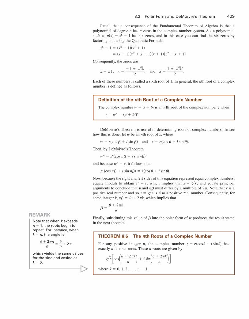
Recall that a consequence of the Fundamental Theorem of Algebra is that a polynomial of degree has zeros in the complex number system. So, a polynomialsuch as has six zeros, and in this case you can find the six zeros by factoring and using the Quadratic Formula.
Consequently, the zeros are
and
Each of these numbers is called a sixth root of 1. In general, the th root of a complexnumber is defined as follows.
DeMoivre’s Theorem is useful in determining roots of complex numbers. To seehow this is done, let be an th root of where
and
Then, by DeMoivre’s Theorem
and because it follows that
Now, because the right and left sides of this equation represent equal complex numbers,equate moduli to obtain which implies that and equate principal arguments to conclude that and must differ by a multiple of Note that is apositive real number and so is also a positive real number. Consequently, forsome integer which implies that
Finally, substituting this value of into the polar form of produces the result statedin the next theorem.
w
�� � 2�k
n .
k, n � � � 2�k,s � n�r
r2�.n�s � n�r ,sn � r,
sn �cos n � i sin n� � r�cos � � i sin ��.
wn � z,
wn � sn�cos n � i sin n�
z � r�cos � � i sin ��.w � s�cos � i sin �
z,nw
n
x �1 ± �3 i
2.x �
�1 ± �3i2
,x � ±1,
� �x � 1��x2 � x � 1��x � 1��x2 � x � 1� x6 � 1 � �x3 � 1��x3 � 1�
p�x� � x6 � 1nn
8.3 Polar Form and DeMoivre’s Theorem 409
REMARK
Note that when exceedsthe roots begin to
repeat. For instance, whenthe angle is
which yields the same valuesfor the sine and cosine ask � 0.
� � 2�nn
��
n� 2�
k � n,
n � 1,k
Definition of the nth Root of a Complex Number
The complex number is an th root of the complex number when
z � wn � �a � bi�n.
znw � a � bi
THEOREM 8.6 The nth Roots of a Complex Number
For any positive integer the complex number has exactly distinct roots. These roots are given by
where k � 0, 1, 2, . . . , n � 1.
n�r �cos�� � 2�kn � � i sin�� � 2�k
n ��nn
z � r �cos � � i sin ��n,
9781133110873_0803.qxp 3/10/12 6:54 AM Page 409

The formula for the th roots of a complexnumber has a nice geometric interpretation, asshown in Figure 8.10. Because the th roots allhave the same modulus (length) they lie on acircle of radius with center at the origin.Furthermore, the roots are equally spacedaround the circle, because successive th rootshave arguments that differ by
You have already found the sixth roots of 1 byfactoring and the Quadratic Formula. Try solvingthe same problem using Theorem 8.6 to get theroots shown in Figure 8.11. When Theorem 8.6 isapplied to the real number 1, the th roots have aspecial name—the th roots of unity.
Finding the nth Roots of a Complex Number
Determine the fourth roots of
SOLUTION
In polar form,
so Then, by applying Theorem 8.6,
Setting and 3,
as shown in Figure 8.12.
Figure 8.12
Imaginaryaxis
Realaxis
13π
π8
π8
9π8
813π
8
9π8cos + i sin
5π8
5π8cos + i sin
cos + i sin
cos + i sin
z4 � cos 13�
8� i sin
13�
8
z3 � cos 9�
8� i sin
9�
8
z2 � cos 5�
8� i sin
5�
8
z1 � cos �
8� i sin
�
8
k � 0, 1, 2,
� cos��
8�
k�
2 � � i sin��
8�
k�
2 �.
i1�4 � 4�1 �cos���24
�2k�
4 � � i sin���24
�2k�
4 ��r � 1 and � � ��2.
i � 1�cos �
2� i sin
�
2�
i.
nn
2��n.n
n
n�r
n�r,n
n
410 Chapter 8 Complex Vector Spaces
rn
2π
2π
n
n
The nth Roots of aComplex Number
Realaxis
Imaginaryaxis
Figure 8.10
Imaginaryaxis
Realaxis
The Sixth Roots of Unity
1−1
1
1
1
1
2
2
2
2
2
2
2
2
3
3
3
3
+
−
+
−
i
i
i
i
−
−
Figure 8.11
REMARK
In Figure 8.12, note that wheneach of the four angles
and ismultiplied by 4, the result is ofthe form ���2� � 2k�.
13��8��8, 5��8, 9��8,
9781133110873_0803.qxp 3/10/12 6:54 AM Page 410

8.3 Exercises 411
8.3 Exercises
Converting to Polar Form In Exercises 1–4, expressthe complex number in polar form.
1. 2.
3. 4.
Graphing and Converting to Polar Form In Exercises5–16, represent the complex number graphically, andgive the polar form of the number. (Use the principalargument.)
5. 6.
7. 8.
9. 10.
11. 7 12. 4
13. 14.
15. 16.
Graphing and Converting to Standard Form InExercises 17–26, represent the complex number graphically, and give the standard form of the number.
17.
18.
19.
20.
21. 22.
23. 24.
25. 26.
Multiplying and Dividing in Polar Form In Exercises27–34, perform the indicated operation and leave theresult in polar form.
27.
28.
29.
30.
31.
32.
33.
34.
Finding Powers of Complex Numbers In Exercises35–44, use DeMoivre’s Theorem to find the indicatedpowers of the complex number. Express the result instandard form.
35. 36.
37. 38.
39.
40.
41.
42.
43.
44.
Finding Square Roots of a Complex Number InExercises 45–52, find the square roots of the complexnumber.
45. 46.
47. 48.
49. 50.
51. 52. 1 � �3 i1 � �3 i
2 � 2i2 � 2i
�6i�3i
5i2i
�5�cos 3�
2� i sin
3�
2 ��4
�2�cos �
2� i sin
�
2��8
�cos 5�
4� i sin
5�
4 �10
�3�cos 5�
6� i sin
5�
6 ��4
�5�cos �
9� i sin
�
9��3
�1 � �3i�3
��3 � i�7��1 � i�10
�2 � 2i�6�1 � i�4
9cos�3��4� � i sin�3��4�5cos����4� � i sin����4�
12cos���3� � i sin���3�3cos���6� � i sin���6�
cos�5��3� � i sin�5��3�cos� � i sin�
2cos�2��3� � i sin�2��3�4[cos�5��6� � i sin�5��6�]
�3�cos �
3� i sin
�
3���1
3 �cos
2�
3� i sin
2�
3 ��0.5�cos� � i sin�� 0.5�cos�� � i sin���
�3
4 �cos �
2� i sin
�
2���6�cos �
4� i sin
�
4���3�cos
�
3� i sin
�
3���4�cos �
6� i sin
�
6��
9�cos � � i sin ��7�cos 0 � i sin 0�
6�cos 5�
6� i sin
5�
6 �4�cos 3�
2� i sin
3�
2 �
8�cos �
6� i sin
�
6�15
4 �cos �
4� i sin
�
4�
3
4 �cos
7�
4� i sin
7�
4 �
3
2 �cos 5�
3� i sin
5�
3 �
5�cos 3�
4� i sin
3�
4 �
2�cos �
2� i sin
�
2�
5 � 2i�1 � 2i
2�2 � i3 � �3 i
�2i6i
52��3 � i ��2�1 � �3i �2 � 2i�2 � 2i
Imaginaryaxis
Realaxis
3i
1
1−1
2
3
Imaginaryaxis
Realaxis
−6 1
2
−2
−2−3−4−5−6
−3
3
Imaginaryaxis
Realaxis
1 + 3i
1 2
1
2
3
−1
Imaginaryaxis
Realaxis
1
−1
−2
2
2 − 2i
9781133110873_0803.qxp 3/10/12 6:54 AM Page 411

412 Chapter 8 Complex Vector Spaces
Finding and Graphing nth Roots In Exercises 53–64,(a) use Theorem 8.6 to find the indicated roots, (b) represent each of the roots graphically, and (c) expresseach of the roots in standard form.
53. Square roots:
54. Square roots:
55. Fourth roots:
56. Fifth roots:
57. Square roots:
58. Fourth roots:
59. Cube roots:
60. Cube roots:
61. Cube roots: 8
62. Fourth roots:
63. Fourth roots: 1
64. Cube roots: 1000
Finding and Graphing Solutions In Exercises 65–72,find all the solutions of the equation and represent yoursolutions graphically.
65. 66.
67. 68.
69. 70.
71. 72.
73. Electrical Engineering In an electric circuit, theformula relates voltage drop current andimpedance where complex numbers can representeach of these quantities. Find the impedance when thevoltage drop is and the current is
75. Proof When provided with two complex numbersand
with prove that
76. Proof Show that the complex conjugate ofis
77. Use the polar forms of and in Exercise 76 to findeach of the following.
(a)
(b)
78. Proof Show that the negative of is
79. Writing
(a) Let
Sketch and in the complex plane.
(b) What is the geometric effect of multiplying a complex number by What is the geometriceffect of dividing by
80. Calculus Recall that the Maclaurin series for sin and cos are
(a) Substitute in the series for and show that
(b) Show that any complex number can beexpressed in polar form as
(c) Prove that if then
(d) Prove the formula
True or False? In Exercises 81 and 82, determinewhether each statement is true or false. If a statement istrue, give a reason or cite an appropriate statement fromthe text. If a statement is false, provide an example thatshows the statement is not true in all cases or cite anappropriate statement from the text.
81. Although the square of the complex number is givenby the absolute value of the complex number is defined as
82. Geometrically, the th roots of any complex number are all equally spaced around the unit circle centered atthe origin.
zn a � bi � �a2 � b2.z � a � bi
�bi�2 � �b2,bi
ei� � �1.
z � re�i�.z � rei�,
z � rei�.z � a � bi
ei� � cos � � i sin �.exx � i�
cos x � 1 �x 2
2!�
x4
4!�
x6
6!� . . . .
sin x � x �x 3
3!�
x5
5!�
x7
7!� . . .
ex � 1 � x �x 2
2!�
x3
3!�
x4
4!� . . .
xx,ex,
i?zi?z
z�iiz,z,
z � r�cos � � i sin �� � 2�cos �
6� i sin
�
6�.
�z � rcos�� � �� � i sin�� � ��.
z � r�cos � � i sin ��z�z, z 0
zz
zz
z � rcos���� � i sin����.z � r�cos � � i sin ��
z1z2
�r1r2
cos��1 � �2� � i sin��1 � �2�.
z2 0,z2 � r2�cos �2 � i sin �2�,z1 � r1�cos �1 � i sin �1�
2 � 4i.5 � 5i
Z,I,V,V � I � Z
x4 � i � 0x 3 � 64i � 0
x4 � 81 � 0x5 � 243 � 0
x3 � 27 � 0x 3 � 1 � 0
x4 � 16i � 0x4 � 256i � 0
81i
�4�2 �1 � i��
1252 �1 � �3i�
625i
�25i
32�cos 5�
6� i sin
5�
6 �
16�cos 4�
3� i sin
4�
3 �
9�cos 2�
3� i sin
2�
3 �
16�cos �
3� i sin
�
3�
74. Use the graph of the roots of acomplex number.
(a) Write each of the roots in trigonometric form.
(b) Identify the complex number whose roots aregiven. Use a graphing utility to verify your results.
(i) (ii)
Realaxis
Imaginaryaxis
45°45°
45°45°
3 3
3 3
30°30°
−11
Realaxis
Imaginaryaxis
2 2
2
9781133110873_0803.qxp 3/10/12 6:54 AM Page 412

Answer Key
Section 8.3
1. 3.
5.
7.
9.
11.
13.
15.
17.
19.
21.
15�2
8�
15�2
8i
123 θ = 4
r = 3.75
1 2 3−2−2−3
Realaxis
Imaginaryaxis
π
3
4�
3�3
4i
1
2
θ = 53
Realaxis
Imaginaryaxis
−2
−2 1 2
32r =
π
2i
1
θ = π2
−1−1
r = 2Realaxis
Imaginaryaxis
1
�5 cos��2.0344� � i sin��2.0344��
1 43
1
34
z = −1 − 2i
−1−3
−4
Realaxis
Imaginaryaxis
2�3�cos �
6� i sin
�
6
1 2 4
12
4z = 3 + 3 i
−1−4−2
−4
Realaxis
Imaginaryaxis
7�cos 0 � i sin 0�
3
6
z = 7
Realaxis
3 6−3−3
−6
Imaginaryaxis
6�cos �
2� i sin
�
2
2
4
Realaxis
Imaginaryaxis
z = 6i
−4
−4
−2 2 4
4�cos��2�
3 � i sin��2�
3 �
123
Realaxis
1 2 3−2−2−3
−3
z = −2 − 2 3 i
Imaginaryaxis
�8�cos��3�
4 � i sin��3�
4 �
1
2
1 2
Realaxis
z = −2 − 2i
Imaginaryaxis
6�cos � � i sin ��8�cos���
4 � i sin���
4 �
9781133110873_08_ANS.qxd 3/10/12 6:58 AM Page A2

23.
25.
7
27. 29.
31.
33. 35. 37.
39. 41. 43. 256
45.
Square roots:
47.
Square roots:
49.
Square roots:
51.
Square roots:
53. (a)
(b)
(c)
55. (a)
(b)
(c)
�3 � i�1 � �3 i��3 � i1 � �3 i
1r = 2
θθ
θ
θ
==
=
=
5
11
4
36
6
3
12
4
3
−1−1
1
Realaxis
Imaginaryaxis
π π
π
π
2�cos 11�
6� i sin
11�
6
2�cos 4�
3� i sin
4�
3
2�cos 5�
6� i sin
5�
6
2�cos �
3� i sin
�
3 �2�3 � 2i2�3 � 2i
2θ
θ
=
= 7
6
6
1
2
−2−2
r = 4Realaxis
Imaginaryaxis
π
π
4�cos 7�
6� i sin
7�
6 4�cos
�
6� i sin
�
6
�2�cos7�
6� i sin
7�
6 � ��62
��22
i
�2�cos�
6� i sin
�
6 ��62
��22
i
1 � �3i � 2�cos�
3� i sin
�
3
81�4�cos15�
8� i sin
15�
8 � 1.554 � 0.644i
81�4�cos7�
8� i sin
7�
8 � �1.554 � 0.644i
2�2i � 2�2�cos7�
4� i sin
7�
4
�3�cos7�
4� i sin
7�
4 ��62
��62
i
�3�cos3�
4� i sin
3�
4 � ��62
��62
i
�3i � 3�cos3�
2� i sin
3�
2
�2�cos5�
4� i sin
5�
4 � �1 � i
�2�cos�
4� i sin
�
4 � 1 � i
2i � 2�cos�
2� i sin
�
2 �
81
2�
81�3
2 i�8
�32i�44�cos �
6� i sin
�
6
12 �cos��
�
6 � i sin���
6 �
0.25�cos 0 � i sin 0�12�cos �
2� i sin
�
2
24 θ = 0
r = 7Realaxis
2 4 6−2−4−4−6
Imaginaryaxis
�4i
1 2 3
123
θ = 32
r = 4
−2−2−1−3
−3
Realaxis
Imaginaryaxis
π
Answer Key
9781133110873_08_ANS.qxd 3/10/12 6:58 AM Page A3

Answer Key
57. (a)
(b)
(c)
59. (a)
(b)
(c)
61. (a)
(b)
(c) 2
63. (a)
(b)
(c) 1
65.
67.
1
1
θ
θ
θ
=
=
=
π
5π
π
3
3
2
3
1
−1
Realaxis
Imaginaryaxis
r = 1
cos 5�
3� i sin
5�
3
cos � � i sin �
cos �
3� i sin
�
3
θ
θ
θ
θ
=
=
=
=
13
5
9
8
8
8
8
4
2
3
1
Realaxis
Imaginaryaxis
r = 42
2−2−2
π
π
π
π
4�cos13�
8� i sin
13�
8 4�cos
9�
8� i sin
9�
8 4�cos
5�
8� i sin
5�
8 4�cos
�
8� i sin
�
8 �i�1i
1
1
θ
θ
θ
θ
= 0
=
=
= π 32
2
1
4
2
3
r = 1
−1
Realaxis
Imaginaryaxis
π
π
cos 3�
2� i sin
3�
2
cos � � i sin �
cos �
2� i sin
�
2
cos 0 � i sin 0
�1 � �3 i�1 � �3 i
1θ
θ
θ
= 0
=
=
4
2
3
3
1
3
2
r = 2
−1−1 1
Realaxis
Imaginaryaxis
π
π
2�cos 4�
3� i sin
4�
3
2�cos 2�
3� i sin
2�
3 2�cos 0 � i sin 0�3.83 � 3.21i�4.70 � 1.71i0.868 � 4.92i
2
4
6 θ
θθ
1
32
=
==
4
1610
9
99
2 4 6−2
−4
−6
r = 5Realaxis
Imaginaryaxis
π
ππ
5�cos 16�
9� i sin
16�
9
5�cos 10�
9� i sin
10�
9
5�cos 4�
9� i sin
4�
9
5�2
2�
5�2
2 i
�5�2
2�
5�2
2 i
2
4
6θ
θ
1
2
=
=
3
7
4
4
2 4 6−2−6
−4
−6
r = 5Realaxis
Imaginaryaxis
π
π
5�cos 7�
4� i sin
7�
4
5�cos 3�
4� i sin
3�
4
9781133110873_08_ANS.qxd 3/10/12 6:58 AM Page A4

69.
71.
73. 75. Proof77. (a) (b)79. (a)
(b) Counterclockwise rotation of clockwise rotation of
81. True
�
2�
2;
−1−2
−2
−3
−3 1 2 3
Realaxis
Imaginaryaxis
z /i = 1 − 3 i
z = 3 + i
iz =−1 + 3 i
cos�2�� � i sin�2��r2
32 �
12i
θ
θ
θ=
=
=
11
76
2
6
3
1
2
−2−2
2
2
r = 4Realaxis
Imaginaryaxis
π
π
π
4�cos 11�
6� i sin
11�
6
4�cos 7�
6� i sin
7�
6
4�cos �
2� i sin
�
2
1 2
2 θθ
θ
θθ
1
2
3
5
4
=
=
= π
==
3
9
7
5
5
5
5
−2
−2 −1
r = 3Realaxis
Imaginaryaxis
π
π
π
π
3�cos 9�
5� i sin
9�
5
3�cos 7�
5� i sin
7�
5 3�cos � � i sin ��
3�cos 3�
5� i sin
3�
5
3�cos �
5� i sin
�
5
Answer Key
9781133110873_08_ANS.qxd 3/10/12 6:58 AM Page A5


8.4 Complex Vector Spaces and Inner Products.
p. 163
8.4 Complex Vector Spaces and Inner Products.
Objective: Represent a vector in Cn by a basis.
Objective: Find the row space and null space of a matrix.
Objective: Solve a system of linear equations.
Objective: Find the Euclidean inner product, Euclidean norm, and Euclidean distance in Cn
A complex vector space is a vector space in which the scalars are complex numbers. The
complex version of Rn is the complex vector space Cn
consisting of ordered n-tuples of complex
numbers
v = (a1 + b1i, a2 + b2i, … an + bni)
We also represent vectors in Cn by their coordinate matrices relative to the standard basis
e1 = (1, 0, 0, …, 0), e2 = (0, 1, 0, …, 0), …, en = (0, 0, 0, …, 1),
v =
iba
iba
iba
nn
22
11
As in of Rn, the operations of vector addition and scalar multiplication in Cn
are performed
component by component.
The dimension of Cn is n. A basis of a subspace V of Cn
is any linearly independent set of vectors
that spans V. If V has dimension d, then any linearly independent set of d vectors in V is a basis
of V. Also, any set of d vectors that spans V is a basis of V.
Example: Is R2 a subspace of the complex vector space C2
over C?
Solution: R2 is a subset of C2
because R2 ={(a1 + b1i, a2 + b2i) where b1 = b2 = 0}. Moreover,

8.4 Complex Vector Spaces and Inner Products.
p. 164
Example: Show that S1 = {v1, v2, v3} = {(i, 2, 0), (2, i, 0), (1 + i, 0, 1 – i)} is a basis for C3.
Solution: Because the dimension of C3 is 3, the set S1 will be a basis if it is linearly
independent.
So we must check that
Example: Write u = (2 – i, 8 – 2i, 5 – i) as a linear combination of the vectors in the set S1 = {v1,
v2, v3} = {(i, 2, 0), (2, i, 0), (1 + i, 0, 1 – i)}, i.e. the same set as in the previous example.
Solution:
Example: Find the dimension of and a basis for
S2 = span{(–2 – 2i, –3i, –9 – 6i), (–1 – i, – 3, –3), (–3 – 2i, –1 + 3i, –6 – 5i)}.
Solution: S2 = the column space of

8.4 Complex Vector Spaces and Inner Products.
p. 165
Example: Find the rank, nullity, and bases for the row space and null space of
Solution:

8.4 Complex Vector Spaces and Inner Products.
p. 166
Example: Solve
Solution:
Let u and v be vectors in Cn. The Euclidean inner product of u and v is given by
u•v = u1v1* + u2v2* + … + unvn* = 𝑢1𝑣1̅̅ ̅ + 𝑢2𝑣2̅̅ ̅ + ⋯ + 𝑢𝑛𝑣𝑛̅̅ ̅
Theorem 8.7 Properties of the Euclidean inner product
Let u, v, and w be vectors in Cn and let k be a complex scalar. Then
1) u•v = (v•u)* = v∙u̅̅ ̅̅ Different from Rn!
2) (u + v)•w = u•w + v•w
3) (k u)•v = k (u•v)
4) u•(k v) = k*(u•v) = �̅�(u∙v) Different from Rn!
5) u•u 0 (This also says that u•u is real.)
6) u•u = 0 if and only if u = 0

8.4 Complex Vector Spaces and Inner Products.
p. 167
The Euclidean norm of u in Cn is ||u|| = uu
The Euclidean distance between u and v in Cn is d(u, v) = ||u – v||
To find a dot product u•v on the TI-89, use
MatrixVector opsdotP(u,v)
To find a dot product u•v in Mathematica, use u.vconj which displays as u.v*
To find a dot product u•v in PocketCAS, use dot(v,u) (PocketCAS takes the complex conjugate of the first vector, rather than the second.)
To find a norm ||v|| on the TI-89, use
MatrixNormsnorm(v)
To find a norm ||v|| in Mathematica, use Norm[v]
To find a norm ||v|| in PocketCAS, use l2norm(v) or norm(v)
Example: Let u = (i, 1, 0), v = (–i, 1, 0), and w = (–2 + 3i, –5 + i, –4 – 6i).
Find ||u||
Find ||w||
Find u•v
Find v•w
Find d(u, w)

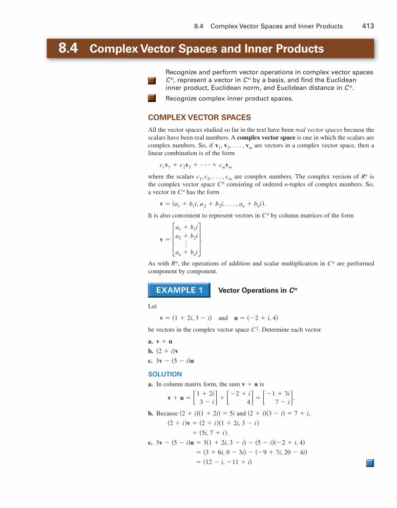
8.4 Complex Vector Spaces and Inner Products 413
8.4 Complex Vector Spaces and Inner Products
Recognize and perform vector operations in complex vector spacesrepresent a vector in by a basis, and find the Euclidean
inner product, Euclidean norm, and Euclidean distance in
Recognize complex inner product spaces.
COMPLEX VECTOR SPACES
All the vector spaces studied so far in the text have been real vector spaces because thescalars have been real numbers. A complex vector space is one in which the scalars arecomplex numbers. So, if are vectors in a complex vector space, then alinear combination is of the form
where the scalars are complex numbers. The complex version of is the complex vector space consisting of ordered -tuples of complex numbers. So,a vector in has the form
It is also convenient to represent vectors in by column matrices of the form
As with the operations of addition and scalar multiplication in are performedcomponent by component.
Vector Operations in
Let
and
be vectors in the complex vector space Determine each vector.
a.
b.
c.
SOLUTION
a. In column matrix form, the sum is
b. Because and
c.
� �12 � i, �11 � i� � �3 � 6i, 9 � 3i� � ��9 � 7i, 20 � 4i�
3v � �5 � i�u � 3�1 � 2i, 3 � i� � �5 � i���2 � i, 4� � �5i, 7 � i �.
�2 � i�v � �2 � i��1 � 2i, 3 � i ��2 � i��3 � i� � 7 � i,�2 � i��1 � 2i� � 5i
v � u � �1 � 2i3 � i� � ��2 � i
4� � ��1 � 3i7 � i�.
v � u
3v � �5 � i�u�2 � i�vv � u
C2.
u � ��2 � i, 4�v � �1 � 2i, 3 � i�
Cn
CnRn,
v � �a1 � b1ia2 � b2i...an � bni
�.
Cn
v � �a1 � b1i, a2 � b2i, . . . , an � bni�.
CnnCn
Rnc1, c2, . . . , cm
c1v1 � c2v2 � � � � � cmvm
v1, v2, . . . , vm
Cn.CnCn,
9781133110873_0804.qxp 3/10/12 6:56 AM Page 413
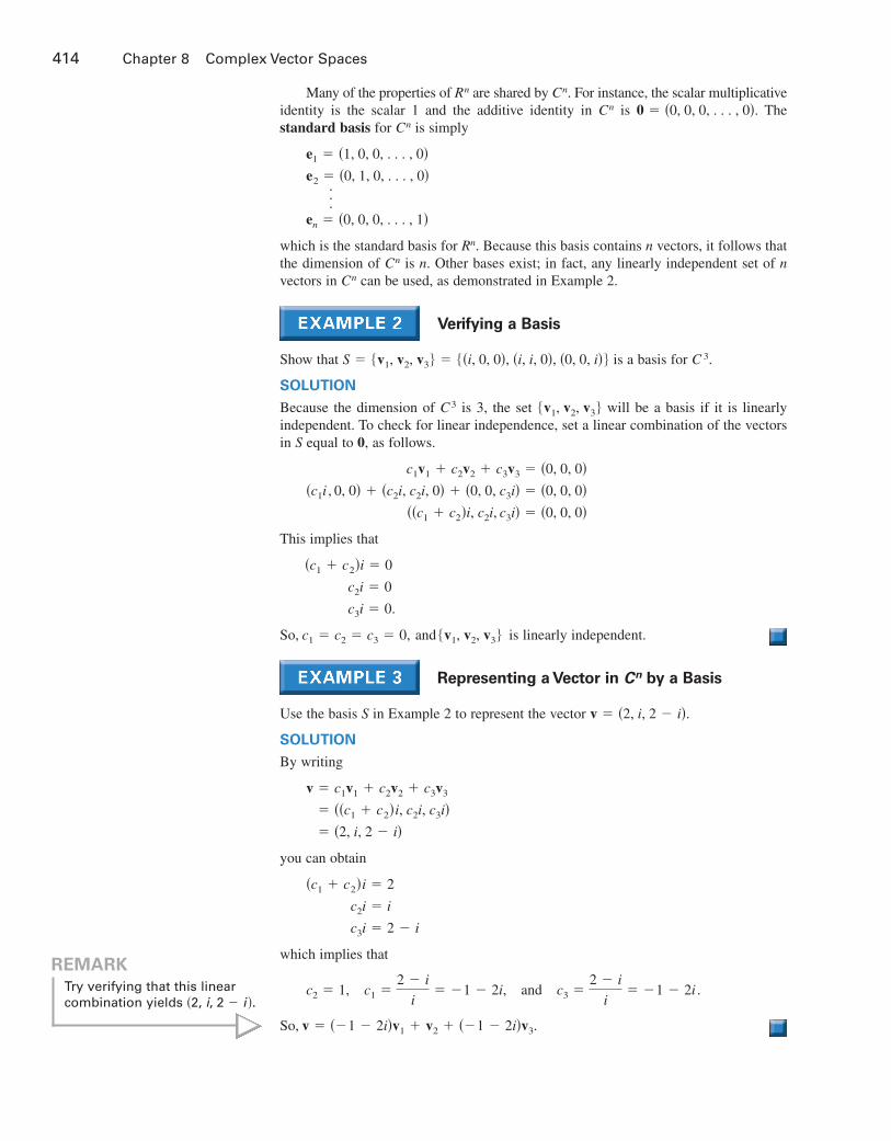
Many of the properties of are shared by For instance, the scalar multiplicativeidentity is the scalar 1 and the additive identity in is The standard basis for is simply
which is the standard basis for Because this basis contains vectors, it follows thatthe dimension of is Other bases exist; in fact, any linearly independent set of vectors in can be used, as demonstrated in Example 2.
Verifying a Basis
Show that is a basis for
SOLUTION
Because the dimension of is 3, the set will be a basis if it is linearly independent. To check for linear independence, set a linear combination of the vectorsin equal to as follows.
This implies that
So, and is linearly independent.
Representing a Vector in by a Basis
Use the basis in Example 2 to represent the vector
SOLUTION
By writing
you can obtain
which implies that
and
So, v � ��1 � 2i�v1 � v2 � ��1 � 2i�v3.
c3 �2 � i
i� �1 � 2i .c1 �
2 � i
i� �1 � 2i,c2 � 1,
c3i � 2 � i
c2i � i
�c1 � c2�i � 2
� �2, i, 2 � i�� ��c1 � c2�i, c2i, c3i�
v � c1v1 � c2v2 � c3v3
v � �2, i, 2 � i�.S
Cn
�v1, v2, v3�c1 � c2 � c3 � 0,
c3i � 0.
c2i � 0
�c1 � c2�i � 0
��c1 � c2�i, c2i, c3i� � �0, 0, 0� �c1i , 0, 0� � �c2i, c2i, 0� � �0, 0, c3i� � �0, 0, 0�
c1v1 � c2v2 � c3v3 � �0, 0, 0�
0,S
�v1, v2, v3�C3
C 3.S � �v1, v2, v3� � ��i, 0, 0�, �i, i, 0�, �0, 0, i��
Cnnn.Cn
nRn.
en � �0, 0, 0, . . . , 1�
.
.
.e2 � �0, 1, 0, . . . , 0�e1 � �1, 0, 0, . . . , 0�
Cn0 � �0, 0, 0, . . . , 0�.Cn
Cn.Rn
414 Chapter 8 Complex Vector Spaces
REMARK
Try verifying that this linearcombination yields �2, i, 2 � i �.
9781133110873_0804.qxp 3/10/12 6:56 AM Page 414
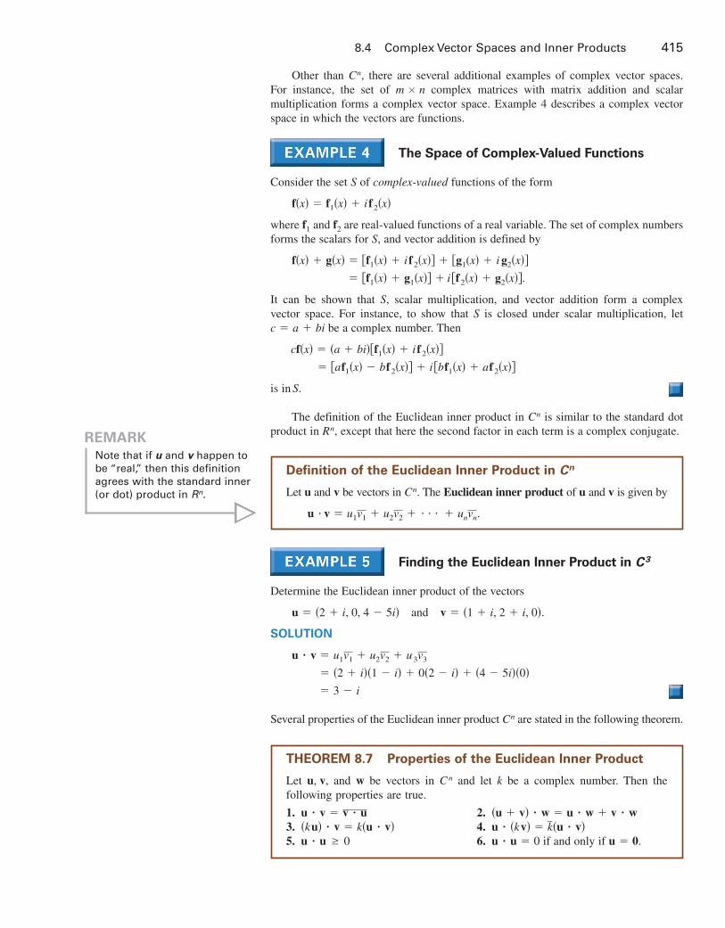
Other than there are several additional examples of complex vector spaces. For instance, the set of complex matrices with matrix addition and scalar multiplication forms a complex vector space. Example 4 describes a complex vectorspace in which the vectors are functions.
The Space of Complex-Valued Functions
Consider the set of complex-valued functions of the form
where and are real-valued functions of a real variable. The set of complex numbersforms the scalars for and vector addition is defined by
It can be shown that scalar multiplication, and vector addition form a complex vector space. For instance, to show that is closed under scalar multiplication, let
be a complex number. Then
is in
The definition of the Euclidean inner product in is similar to the standard dotproduct in except that here the second factor in each term is a complex conjugate.
Finding the Euclidean Inner Product in
Determine the Euclidean inner product of the vectors
and
SOLUTION
Several properties of the Euclidean inner product are stated in the following theorem.Cn
� 3 � i
� �2 � i��1 � i� � 0�2 � i� � �4 � 5i��0� u � v � u1v1 � u2v2 � u3v3
v � �1 � i, 2 � i, 0�.u � �2 � i, 0, 4 � 5i�
C3
Rn,Cn
S.
� �af1�x� � bf2�x� � i�bf1�x� � af2�x� cf�x� � �a � bi��f1�x� � if2�x�
c � a � biS
S,
� �f1�x� � g1�x� � i�f2�x� � g2�x�. f�x� � g�x� � �f1�x� � if2�x� � �g1(x� � i g2�x�
S,f2f1
f�x� � f1�x� � if2�x�
S
m � nCn,
8.4 Complex Vector Spaces and Inner Products 415
REMARK
Note that if and happen tobe “real,” then this definitionagrees with the standard inner(or dot) product in Rn.
vu
THEOREM 8.7 Properties of the Euclidean Inner Product
Let and be vectors in and let be a complex number. Then the following properties are true.
1. 2.3. 4.5. 6. if and only if u � 0.u � u � 0u � u � 0
u � �kv� � k�u � v��ku� � v � k�u � v��u � v� � w � u � w � v � wu � v � v � u
kCnwu, v,
Definition of the Euclidean Inner Product in
Let and be vectors in The Euclidean inner product of and is given by
u � v � u1v1 � u2v2 � � � � � unvn.
vuCn.vu
Cn
9781133110873_0804.qxp 3/10/12 6:56 AM Page 415
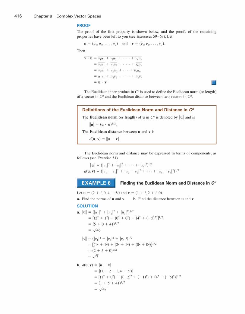
416 Chapter 8 Complex Vector Spaces
Definitions of the Euclidean Norm and Distance in
The Euclidean norm (or length) of in is denoted by and is
The Euclidean distance between and is
d�u, v� � u � v .
vu
u � �u � u�1�2.
uCnu
Cn
PROOF
The proof of the first property is shown below, and the proofs of the remaining properties have been left to you (see Exercises 59–63). Let
and
Then
The Euclidean inner product in is used to define the Euclidean norm (or length)of a vector in and the Euclidean distance between two vectors in .
The Euclidean norm and distance may be expressed in terms of components, asfollows (see Exercise 51).
Finding the Euclidean Norm and Distance in
Let and
a. Find the norms of and b. Find the distance between and
SOLUTION
a.
b.
� �47
� �1 � 5 � 41�1�2
� ��12 � 02� � ���2�2 � ��1�2� � �42 � ��5�2�1�2
� �1, �2 � i, 4 � 5i� d�u, v� � u � v
� �7
� �2 � 5 � 0�1�2
� ��12 � 12� � �22 � 12� � �02 � 02�1�2
v � � v1 2 � v2 2 � v3 2�1�2
� �46
� �5 � 0 � 41�1�2
� ��22 � 12� � �02 � 02� � �42 � ��5�2�1�2
u � � u1 2 � u2 2 � u3 2�1�2
v.uv.u
v � �1 � i, 2 � i, 0�.u � �2 � i, 0, 4 � 5i�
Cn
d�u, v� � � u1 � v1 2 � u2 � v2 2 � . . . � un � vn 2�1�2
u � � u1 2 � u2 2 � . . . � un 2�1�2
CnCnCn
� u � v.
� u1v1 � u2v2 � � � � � unvn
� v1u1 � v2u2 � . . . � vnun
� v1u1 � v2u2 � . . . � vnun
v � u � v1u1 � v2u2 � . . . � vnun
v � �v1, v2, . . . , vn �.u � �u1, u2, . . . , un �
9781133110873_0804.qxp 3/10/12 6:56 AM Page 416

COMPLEX INNER PRODUCT SPACES
The Euclidean inner product is the most commonly used inner product in . On occasion,however, it is useful to consider other inner products. To generalize the notion of aninner product, use the properties listed in Theorem 8.7.
A complex vector space with a complex inner product is called a complex inner product space or unitary space.
A Complex Inner Product Space
Let and be vectors in the complex space Show that thefunction defined by
is a complex inner product.
SOLUTION
Verify the four properties of a complex inner product, as follows.
1.
2.
3.
4.
Moreover, if and only if
Because all the properties hold, is a complex inner product.�u, v�
u1 � u2 � 0.�u, u� � 0
�u, u� � u1u1 � 2u2u2 � u1 2 � 2 u2 2 � 0
�ku, v� � �ku1�v1 � 2�ku2�v2 � k�u1v1 � 2u2v2 � � k �u, v� � �u, w� � �v, w�� �u1w1 � 2u2w2 � � �v1w1 � 2v2w2 �
�u � v, w� � �u1 � v1�w1 � 2�u2 � v2�w2
� u1v1 � 2u2v2 � �u, v�v1u1 � 2v2u2�v, u� �
�u, v� � u1v1 � 2u2v2
C2.v � �v1, v2�u � �u1, u2�
Cn
8.4 Complex Vector Spaces and Inner Products 417
Definition of a Complex Inner Product
Let and be vectors in a complex vector space. A function that associates and with the complex number is called a complex inner product whenit satisfies the following properties.
1.2.3.4. and if and only if u � 0.�u, u� � 0�u, u� � 0
�ku, v� � k�u, v��u � v, w� � �u, w� � �v, w��u, v� � �v, u�
�u, v�vuvu
LINEAR ALGEBRA APPLIED
Complex vector spaces and inner products have an importantapplication called the Fourier transform, which decomposes a function into a sum of orthogonal basis functions. The givenfunction is projected onto the standard basis functions for varying frequencies to get the Fourier amplitudes foreach frequency. Like Fourier coefficients and the Fourier approximation, this transform is named after the Frenchmathematician Jean-Baptiste Joseph Fourier (1768–1830).
The Fourier transform is integral to the study of signal processing. To understand the basic premise of this transform, imagine striking two piano keys simultaneously.Your ear receives only one signal, the mixed sound of thetwo notes, and yet your brain is able to separate the notes.The Fourier transform gives a mathematical way to take asignal and separate out its frequency components.
Eliks/Shutterstock.com
9781133110873_0804.qxp 3/10/12 6:56 AM Page 417
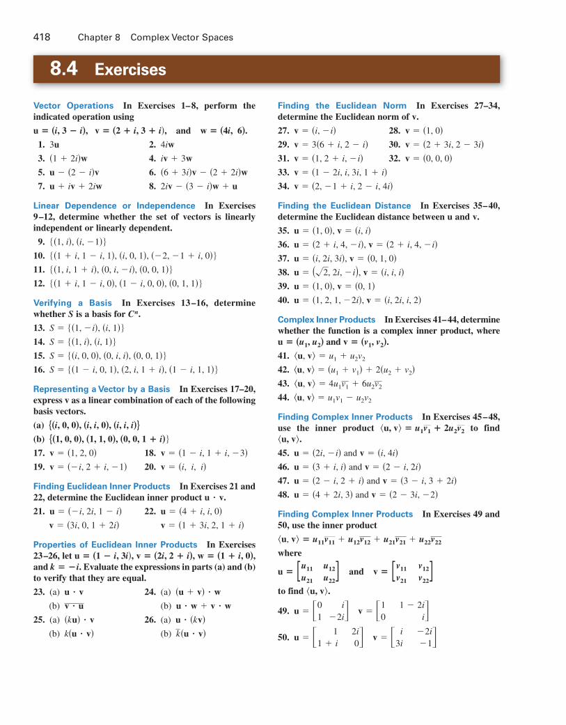
418 Chapter 8 Complex Vector Spaces
8.4 Exercises
Vector Operations In Exercises 1–8, perform the indicated operation using
and
1. 2.
3. 4.
5. 6.
7. 8.
Linear Dependence or Independence In Exercises9–12, determine whether the set of vectors is linearlyindependent or linearly dependent.
9.
10.
11.
12.
Verifying a Basis In Exercises 13–16, determinewhether is a basis for
13.
14.
15.
16.
Representing a Vector by a Basis In Exercises 17–20,express as a linear combination of each of the followingbasis vectors.
(a)
(b)
17. 18.
19. 20.
Finding Euclidean Inner Products In Exercises 21 and22, determine the Euclidean inner product
21. 22.
Properties of Euclidean Inner Products In Exercises23–26, let and Evaluate the expressions in parts (a) and (b)to verify that they are equal.
23. (a) 24. (a)
(b) (b)
25. (a) 26. (a)
(b) (b)
Finding the Euclidean Norm In Exercises 27–34,determine the Euclidean norm of
27. 28.
29. 30.
31. 32.
33.
34.
Finding the Euclidean Distance In Exercises 35–40,determine the Euclidean distance between and
35.
36.
37.
38.
39.
40.
Complex Inner Products In Exercises 41–44, determinewhether the function is a complex inner product, where
and
41.
42.
43.
44.
Finding Complex Inner Products In Exercises 45–48,use the inner product to find
45. and
46. and
47. and
48. and
Finding Complex Inner Products In Exercises 49 and50, use the inner product
where
and
to find
49.
50. v � � i3i
�2i�1�u � � 1
1 � i2i0�
v � �10
1 � 2ii�u � �0
1i
�2i��u, v�.
v � [v11
v21
v12
v22]u � [u11
u21
u12
u22]
�u, v� � u11v11 � u12v12 � u21v21 � u22v22
v � �2 � 3i, �2�u � �4 � 2i, 3�v � �3 � i, 3 � 2i�u � �2 � i, 2 � i�
v � �2 � i, 2i�u � �3 � i, i�v � �i, 4i�u � �2i, �i�
�u, v�.�u, v� � u1v1 � 2u2v2
�u, v� � u1v1 � u2v2
�u, v� � 4u1v1 � 6u2v2
�u, v� � �u1 � v1� � 2�u2 � v2��u, v� � u1 � u2v2
v � �v1, v2�.u � �u1, u2�
u � �1, 2, 1, �2i�, v � �i, 2i, i, 2�u � �1, 0�, v � �0, 1�u � ��2, 2i, �i�, v � �i, i, i�u � �i, 2i, 3i�, v � �0, 1, 0�u � �2 � i, 4, �i�, v � �2 � i, 4, �i�u � �1, 0�, v � �i, i�
v.u
v � �2, �1 � i, 2 � i, 4i�v � �1 � 2i, i, 3i, 1 � i�
v � �0, 0, 0�v � �1, 2 � i, �i�v � �2 � 3i, 2 � 3i�v � 3�6 � i, 2 � i�v � �1, 0�v � �i, �i�
v.
k�u � v�k�u � v�u � �kv��ku� � v
u � w � v � wv � u
�u � v� � wu � v
k � �i.w � �1 � i, 0�,v � �2i, 2 � i�,u � �1 � i, 3i�,
v � �1 � 3i, 2, 1 � i�v � �3i, 0, 1 � 2i�u � �4 � i, i, 0�u � ��i, 2i, 1 � i�
u � v.
v � �i, i, i�v � ��i, 2 � i, �1�v � �1 � i, 1 � i, �3�v � �1, 2, 0�
{�1, 0, 0�, �1, 1, 0�, �0, 0, 1 � i��{�i, 0, 0�, �i, i, 0�, �i, i, i�}
v
S � ��1 � i, 0, 1�, �2, i, 1 � i�, �1 � i, 1, 1��S � ��i, 0, 0�, �0, i, i�, �0, 0, 1��S � ��1, i�, �i, 1��S � ��1, �i�, �i, 1��
Cn.S
��1 � i, 1 � i, 0�, �1 � i, 0, 0�, �0, 1, 1����1, i, 1 � i�, �0, i, �i�, �0, 0, 1����1 � i, 1 � i, 1�, �i, 0, 1�, ��2, �1 � i, 0����1, i�, �i, �1��
2iv � �3 � i�w � uu � iv � 2iw
�6 � 3i�v � �2 � 2i�wu � �2 � i�viv � 3w�1 � 2i�w4iw3u
w � �4i, 6�.u � �i, 3 � i�, v � �2 � i, 3 � i�,
9781133110873_0804.qxp 3/10/12 6:56 AM Page 418
8.4 Exercises 419
51. Let
(a) Use the definitions of Euclidean norm and Euclideaninner product to show that
(b) Use the results of part (a) to show that
53. Let and If and the set is not a basis for what doesthis imply about and
54. Let and Determine a vectorsuch that is a basis for
Properties of Complex Inner Products In Exercises55–58, verify the statement using the properties of acomplex inner product.
55.
56.
57.
58.
Proof In Exercises 59–63, prove the property, whereand are vectors in and is a complex number.
59.
60.
61.
62.
63. if and only if
64. Writing Let be a complex inner product and letbe a complex number. How are and
related?
Finding a Linear Transformation In Exercises 65 and66, determine the linear transformation thathas the given characteristics.
65.
66.
Finding an Image and a Preimage In Exercises 67–70,the linear transformation is shown by
Find the image of and the preimage of
67.
68.
69.
70.
71. Find the kernel of the linear transformation in Exercise 68.
72. Find the kernel of the linear transformation in Exercise 69.
Finding an Image In Exercises 73 and 74, find theimage of for the indicated composition, where
and are the matrices below.
and
73. 74.
75. Determine which of the sets below are subspaces of thevector space of complex matrices.
(a) The set of symmetric matrices.
(b) The set of matrices satisfying
(c) The set of matrices in which all entries arereal.
(d) The set of diagonal matrices.
76. Determine which of the sets below are subspaces ofthe vector space of complex-valued functions (seeExample 4).
(a) The set of all functions satisfying
(b) The set of all functions satisfying
(c) The set of all functions satisfying
True or False? In Exercises 77 and 78, determinewhether each statement is true or false. If a statement istrue, give a reason or cite an appropriate statement fromthe text. If a statement is false, provide an example thatshows the statement is not true in all cases or cite anappropriate statement from the text.
77. Using the Euclidean inner product of and in
78. The Euclidean norm of in denoted by is�u � u�2.
uCnu
u � v � u1v1 � u2v2 � . . . � unvn.Cn,vu
f�i� � f��i�.f
f �0� � 1.f
f�i� � 0.f
2 � 2
2 � 2
�A�T � A.A2 � 2
2 � 2
2 � 2
T1 � T2T2 � T1
T2 � [�ii
i�i]T1 � [0
ii0]
T2T1
v � �i, i�
w � �1 � i1 � i
i�v � �250�,A � �
0i0
1 i i
1�1 0�,
w � �2
2i3i�v � � 2 � i
3 � 2i�,A � �1ii
00i�,
w � �11�v � �
i0
1 � i�,A � �0i
i0
10�,
w � �00�v � �1 � i
1 � i�,A � �1i
0i�,
w.vT�v� � Av.T : Cm → Cn
T�0, i� � �0, �i�T�i, 0� � �2 � i, 1�T�0, 1� � �0, �i�T�1, 0� � �2 � i, 1�
T : Cm → Cn
�u, kv��u, v�k�u, v�
u � 0.u � u � 0
u � u � 0
u � �kv� � k�u � v��ku� � v � k�u � v��u � v� � w � u � w � v � w
kCnwu, v,
� k�u, v��u, kv��u, v� � �u, v� � �v, 2u��u, 0� � 0
�u, kv � w� � k�u, v� � �u, w�
C3.�v1, v2, v3�v3
v2 � �1, 0, 1�.v1 � �i, i, i�z3?z1, z2,
C3,�v1, v2, v3�v3 � �z1, z2, z3�v2 � �i, i, 0�.v1 � �i, 0, 0�
� . . . � un � vn 2�1�2.
d�u, v� � � u1 � v1 2 � u2 � v2 2
u � � u1 2 � u2 2 � . . . � un 2�1�2.
u � �a1 � b1i, a2 � b2i, . . . , an � bni�.
52. The complex Euclidean innerproduct of and is sometimes called the complex dot product. Compare the properties ofthe complex dot product in and those of the dotproduct in
(a) Which properties are the same? Which propertiesare different?
(b) Explain the reasons for the differences.
Rn.Cn
vu
9781133110873_0804.qxp 3/10/12 6:56 AM Page 419

Section 8.4 1. � 3.5. 7.9. Linearly dependent 11. Linearly independent
13. is not a basis for 15. is a basis for17. (a)
(b)
19. (a)
(b)
21.23. (a)
(b)The expressions are equal.
25. (a)(b)The expressions are equal.
27. 29. 31. 33. 35.37. 39. 41. Not a complex inner product43. A complex inner product 45. 47.49. 51. (a) and (b) Proofs53. and z2 can be any complex numbers.55.
57.
59–63. Proofs 65.
67. � , � 69.
71. where
73. 75. (a), (b), and (d) are subspaces.
77. False.u � v � u1v1 � u2v2 � . . . � unvn
�0
0� t � R�ker�T� � ��0, t, �ti�,
�2 � i
1 � 2i
�1 � 5i�, �2
1�1 � i
2i� �00
Tu�u1
2� � �2 � i
10
�i u��u1
2�
� �v, u � u� � �v, 2u�
�u, v� � �u, v� � �v, u� � �v, u�
� k�u, v� � �u, w� �u, kv � w� � �u, kv� � �u, w�z3 � 0, z1
�4 � i23 � 3i�6
�2�15�3�17�73�42�2
4 � i4 � i
1 � 4i1 � 4i
�4 � 3i
12
12 �� � i��0, 0, 1 � i�
�2 � i��1, 1, 0� �
�1 � 3i��i, i, 0� � i�i, i, i� ��i, 2 � i, �1� � ��2 � 2i��1, 0, 0� �
��i, 2 � i, �1� � ��2 � 2i��i, 0, 0� �
�1, 2, 0� � i�i, 0, 0� � 2i�i, i, 0� � 0�i, i, i��1, 2, 0� � ��1, 0, 0� � 2�1, 1, 0� � 0�0, 0, 1 � i�
C 3.S C 2.S
��9 � 3i, 2 � 14i���5 � i, �4���8 � 4i, 6 � 12i��3i, 9 3i�
Answer Key

Chapter 6: Linear Transformations.
6.1 Introduction to Linear Transformations.
p. 169
S*
And T()*
Chapter 6: Linear Transformations.
6.1 Introduction to Linear Transformations.
Objective: Find the image and preimage of a function
Objective: Show that a function is a linear transformation.
Recognize and describe some common linear transformations.
A function T: V W maps a vector space V to a W. V is the domain and W is the codomain of
T. If v V and w W such that T (v) = w then w is the image of v under T. The set of all
images of vectors in V is called the range of T. The set of all vectors in V such that T (v) = w is
the preimage of w.
preimage domain v V
image range codomain w range W
Let V and W be vector spaces. Then the function (or map) T : V W is a linear transformation
when the following two properties are true for all v V and w W and for any scalar c.
1) T(u + v) = T(u) + T(v)
2) T(cu) = c T(u)
A linear transformation is “operation preserving” because applying an operation in V (before T )
gives the same result as applying the corresponding operation in W (after T ).
T(u + v) = T(u) + T(v) T(cu) = c T(u)
Example: Show that T : R2 R2
given by T(v1, v2) = (v1 – v2, v1 + v2) is a linear transformation,
find the image of (13, –4), and find the preimage of (2, 8). [Note: technically, we should write
T((v1, v2)) because v = (v1, v2).]
addition
in Vaddition
in W
scalar
multiplication
in W
scalar
multiplication
in V
T T T T

Chapter 6: Linear Transformations.
6.1 Introduction to Linear Transformations.
p. 170
S*
S*
Solution: T(u + v) = T(u1 + v1, u2 + v2)
= ((u1 + v1) – (u2 + v2), (u1 + v1) + (u2 + v2))
= (u1 – u2, u1 + u2) + (v1 – v2, v1 + v2)
= T(u) + T(v)
T(cu) = T(cv1, cv2)
(cv1 – cv2, cv1 + cv2)
(c(v1 – v2), c(v1 + v2))
c (v1 – v2, v1 + v2)
=c T(u)
Image of (13, –4):
T(13, –4) = (13 + (–4), 13 – (–4)) = (9, 17)
Preimage of (2, 8): T(v1, v2) = (v1 – v2, v1 + v2) = (2, 8)
v1 – v2 = 2 2 v1 = 10
v1 + v2 = 8 –2 v2 = –6
(v1, v2) = (5, 3)
Example: Show that f : R R given by f (x) = x2 is not a linear transformation.
Solution: f (x + y) = (x + y)2 = x
2 + 2xy + y
2.
Usually, this is not equal to f (x) + f (y) = x2 + y
2.
In particular, a specific counterexample is f (1 + 1) = 4, but f (1) + f (1) = 2.
Example: Show that f : R R given by f (x) = x + 1 is not a linear transformation.
Solution: f (x + y) = x + y + 1, which is never equal to f (x) + f (y) = x + 1 + y + 1.
[However, f (x) = x + 1 is a linear function, because its graph is a straight line.]
Two simple linear transformations are the zero transformation T : V W, T(v) = 0 for all v V
and the identity transformation T : V V, T(v) = v for all v V.
Theorem 6.1 Properties of Linear Transformations
Let T: V W be a linear transformation, and u and v be vectors in V. Then
1) T(0) = 0
2) T(–v) = –T(v)
3) T(u – v) = T(u) – T(v)
4) If v = c1v1 + c2v2 + …+ cnvn then
T(v) = T(c1v1 + c2v2 + …+ cnvn) = c1T(v1) + c2T(v2) + …+ cnT(vn)

Chapter 6: Linear Transformations.
6.1 Introduction to Linear Transformations.
p. 171
Proof:
1) T(0) =
2) T(–v) =
3) T(u – v) =
4) Prove T(c1v1 + c2v2 + …+ cnvn) = c1T(v1) + c2T(v2) + …+ cnT(vn) by induction:
T(c1v1) = c1T(v1) by the second property of linearity
Suppose T(c1v1 + c2v2 + …+ cnvn) = c1T(v1) + c2T(v2) + …+ cnT(vn).
Then T(c1v1 + c2v2 + …+ cnvn + cn+1vn+1)
= T(c1v1 + c2v2 + …+ cnvn) + T(cn+1vn+1) by the first property of linearity
= c1T(v1) + c2T(v2) + …+ cnT(vn) + T(cn+1vn+1) by supposition
= c1T(v1) + c2T(v2) + …+ cnT(vn) + cn+1T(vn+1) by the second property of linearity
Property 4 of Theorem 6.1 tells us that a linear transformation is completely determined by its
action on a basis for V. In other words, if {v1, v2, …, vn} is a basis for V and if T(v1), T(v2), …,
T(vn) are known, then T(v) is determined for any v V.
Example: Let T: R3 R3
be a linear transformation such that
T(1, 0, 0) = (3, 1, 4) T(0, 1, 0) = (1, 5, 9) T(0, 0, 1) = (2, 6, 5)
Find T(2, 7, 1).
Solution: T(2, 7, 1) = 2 T(1, 0, 0) + 7 T(0, 1, 0) + 1 T(0, 0, 1)
= 2(3, 1, 4) + 7(1, 5, 9) + 1(2, 6, 5)
= (17, 46, 51)

Chapter 6: Linear Transformations.
6.1 Introduction to Linear Transformations.
p. 172
Example: Let T: R2 R3
the function such that
T(v) = Av =
76
34
57
2
1
v
v
Show that T is a linear function. Find T(1, 0) and T(0, 1).
Solution:
For any u and v in R2, T(u + v) = A(u + v) = Au + Av = T(u) + T(v).
Also, for any v in R2 and any scalar c, T(cv) = A(cv) = c(Av) = cT(v).
T(1, 0) =
76
34
57
0
1 =
6
4
7
= (7, –4, –6)
and
T(0, 1) =
76
34
57
1
0 =
7
3
5
= (5, –3, –7)
Notice that T(1, 0) and T(0, 1) are just the two columns of A.
Theorem 6.2: The Linear Transformation Given by a Matrix
Let A be an mn matrix. The function T: Rn Rm
the defined by T(v) = Av is a linear
transformation. Vectors in Rn are represented by n1 (column) matrices and vectors in Rm
are
represented by m1 (column) matrices.
T(v) =
nmmnmm
n
n
aaa
aaa
aaa
21
22221
11211
1
2
1
nnv
v
v
=
12211
2222121
1212111
mnmnmm
nn
nn
vavava
vavava
vavava
Example: Rotation. We show that the linear transformation T: R2 R2
represented by the
matrix
A =
)cos()sin(
)sin()cos(
rotates every vector in R2
counterclockwise by an angle about the
origin.
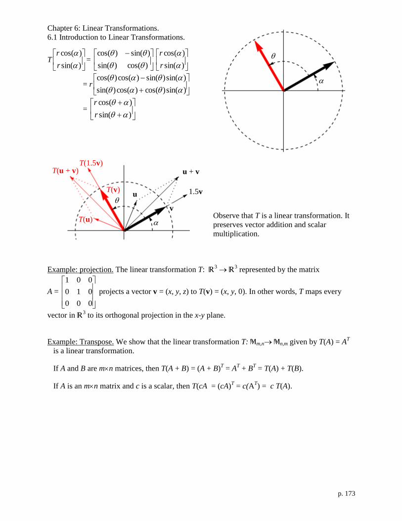
Chapter 6: Linear Transformations.
6.1 Introduction to Linear Transformations.
p. 173
T
)sin(
)cos(
r
r=
)cos()sin(
)sin()cos(
)sin(
)cos(
r
r
= r
)sin()cos()cos()sin(
)sin()sin()cos()cos(
=
)sin(
)cos(
r
r
Observe that T is a linear transformation. It
preserves vector addition and scalar
multiplication.
Example: projection. The linear transformation T: R3 R3
represented by the matrix
A =
000
010
001
projects a vector v = (x, y, z) to T(v) = (x, y, 0). In other words, T maps every
vector in R3 to its orthogonal projection in the x-y plane.
Example: Transpose. We show that the linear transformation T: Mm,n Mn,m given by T(A) = AT
is a linear transformation.
If A and B are mn matrices, then T(A + B) = (A + B)T = A
T + B
T = T(A) + T(B).
If A is an mn matrix and c is a scalar, then T(cA = (cA)T = c(A
T) = c T(A).
u
v
1.5v
u + v
T(u)
T(v)
T(1.5v) T(u + v)
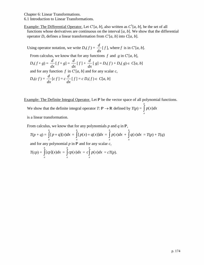
Chapter 6: Linear Transformations.
6.1 Introduction to Linear Transformations.
p. 174
Example: The Differential Operator. Let C[a, b], also written as C1[a, b], be the set of all
functions whose derivatives are continuous on the interval [a, b]. We show that the differential
operator Dx defines a linear transformation from C[a, b] into C[a, b].
Using operator notation, we write Dx( f ) = dx
d[ f ], where f is in C[a, b].
From calculus, we know that for any functions f and g in C[a, b],
Dx( f + g) = dx
d[ f + g] =
dx
d[ f ] +
dx
d[ g] = Dx( f ) + Dx( g) C[a, b]
and for any function f in C[a, b] and for any scalar c,
Dx(c f ) = dx
d[c f ] = c
dx
d[ f ] = c Dx( f ) C[a, b]
Example: The Definite Integral Operator. Let P be the vector space of all polynomial functions.
We show that the definite integral operator T: P R defined by T(p) = b
a
dxxp )(
is a linear transformation.
From calculus, we know that for any polynomials p and q in P,
T(p + q) =
b
a
dxxqp )]([ =
b
a
dxxqxp )]()([ = b
a
dxxp )( + b
a
dxxq )( = T(p) + T(q)
and for any polynomial p in P and for any scalar c,
T(cp) = b
a
dxxcp )]([ = b
a
dxxcp )( = b
a
dxxpc )( = cT(p).

Chapter 6: Linear Transformations.
6.2 The Kernel and Range of a Linear Transformation.
p. 175
S*
6.2 The Kernel and Range of a Linear Transformation.
Objective: Find the kernel of a linear transformation.
Objective: Find a basis for the range, the rank, and the nullity of a linear transformation.
Objective: Determine whether a linear transformation is one-to-one or onto.
Objective: Prove basic results about one-to-one and/or onto linear transformations.
Objective: Determine whether vector spaces are isomorphic.
Let T: V W be a linear transformation. Then the set of all vectors v in V such that T(v) = 0 is
the kernel of T and is denoted by ker(T).
Remember that for any linear transformation, T(0) = 0, so ker(T) always contains 0.
Example Find the kernel of the projection T: R3 R3
defined by T(x, y, z) = (x, y, 0).
Solution: The solution to T(x, y, z) = (0, 0, 0) is x = 0, y = 0. So ker(T) = {(0, 0, z): z R}
Example Find the kernel of the zero transformation T: V W defined T(v) = 0.
Solution: T(v) = 0 is true for all v V so ker(T) = V
Example Find the kernel of the identity transformation T: V V defined T(v) = v.
Solution: T(v) = 0 means v = 0 so ker(T) = {0}.
Example Find the kernel of the linear transformation T: R3 R2
defined by
T(x1, x2, x3) = (5x1 – 4x2 – 6x3, 4x2 –8x3).
Solution: T(x1, x2, x3) = (0, 0) yields the system
084
0645
32
321
xx
xxx
0840
0645rref
0210
0015
14
which has the solution x3 = t, x2 = 2t, x1 = t5
14 so ker(T) = {( t5
14 , 2t, t): t R}
Theorem 6.3: The Kernel of T: V W is a Subspace of V
The kernel of a linear transformation T: V W is a subspace of the domain V.
Proof: 0 ker(T) so ker(T) is not empty.
If u, v ker(T), then T(u) = 0 and T(v) = 0
so T(u + v) = T(u) + T(v) = 0 so u + v ker(T)
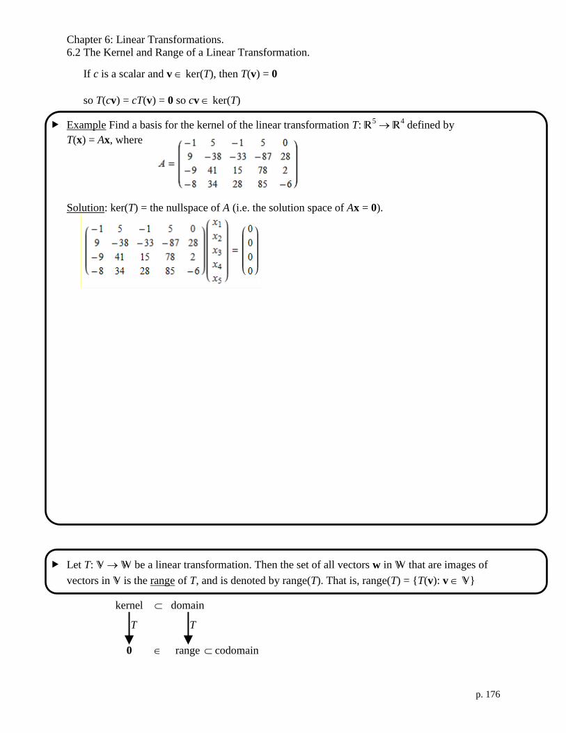
Chapter 6: Linear Transformations.
6.2 The Kernel and Range of a Linear Transformation.
p. 176
S*
S*
If c is a scalar and v ker(T), then T(v) = 0
so T(cv) = cT(v) = 0 so cv ker(T)
Example Find a basis for the kernel of the linear transformation T: R5 R4
defined by
T(x) = Ax, where
Solution: ker(T) = the nullspace of A (i.e. the solution space of Ax = 0).
Let T: V W be a linear transformation. Then the set of all vectors w in W that are images of
vectors in V is the range of T, and is denoted by range(T). That is, range(T) = {T(v): v V}
kernel domain
0 range codomain
T T

Chapter 6: Linear Transformations.
6.2 The Kernel and Range of a Linear Transformation.
p. 177
S*
S*
Theorem 6.4: The Range of T: V W is a Subspace of W
The range of a linear transformation T: V W is a subspace of the codomain W.
Proof: 0 range(T) because T(0) = 0, so range(T) is not empty.
If T(u) and T(v) are vectors in range(T), then u and v are vectors in V. V is closed under
addition, so u + v V, so T(u + v) range(T). T(u + v) = T(u) + T(v), so
T(u) and T(v) range(T) implies that T(u) + T(v) range(T).
Let c be a scalar and T(v) range(T) Then v V. Since V is closed under scalar
multiplication, cv V, so T(cv) range(T). T(cv) = cT(v), so
Let c be a scalar and T(v) range(T) implies that cT(v) range(T).
so T(cv) = cT(v) = 0 so cv ker(T)
Example Find a basis for the range of the linear transformation T: R5 R4
defined by
T(x) = Ax, where
Solution: range(T) = the column space of A.
Let T: V W be a linear transformation. The dimension of the kernel of T is called the nullity
of T and is denoted by nullity(T), the dimension of the range of T is called the rank of T and is
denoted by rank(T).

Chapter 6: Linear Transformations.
6.2 The Kernel and Range of a Linear Transformation.
p. 178
S*
S*
S*
Theorem 6.5: The Sum of Rank and Nullity
Let T: V W be a linear transformation from the n-dimensional vector space V into a vector
space W. Then
rank(T ) + nullity(T ) = n
i.e. dim(range(T )) + dim(kernel(T )) = dim(domain(T ))
Example Find the rank and nullity of the linear transformation T: R8 R5
defined by
T(x) = Ax, where
Solution:
A function T: V W is one-to-one (injective) if and only if every vector in the range of T has a
single (unique) preimage. An equivalent definition is that T is one-to one if and only if T(u) =
T(v) implies that u = v.
A function T: V W is onto (surjective) if and only if the range of T is W (the codomain of T ).
And equivalent definition is that that T is one-to one if and only if every element in W has a
preimage in V.
Example: T: R2 R3
defined by T(x, y) = (x, y, x) is one-to-one
but not onto (points with z x have no preimage).
Example: The projection T: R3 R2
defined by T(x, y, z) = (x, y) is onto
but not one-to-one.

Chapter 6: Linear Transformations.
6.2 The Kernel and Range of a Linear Transformation.
p. 179
S*
Example: The projection T: R2 R2
defined by T(x, y) = (x – 2y, 3x – 6y) = (x – 2y) (1, 3)
is neither one-to-one (because there are many different (x, y) pairs that give the same value of x –
2y ) nor onto (because points with y 3x are not in the range of T).
Example: The transformation T: Rn R n
defined by T(v) = Av, where A is an invertible
matrix, is one-to-one and onto.
T is one-to-one because T(u) = T(v) implies Au = Av. Since A is invertible, we can pre-multiply
by A–1
to obtain A–1
Au = A–1
Av or u = v.
T is onto because the rank of an invertible nn matrix (namely, A) is n. So we also have
rank(T ) = n. By Theorem 6.7 (below), T is onto because its rank equals the dimension of its
codomain.
Theorem 6.6: One-to-One Linear Transformations
Let T: V W be a linear transformation. Then T is one-to-one if and only if ker(T ) = {0}.
Proof
If T is one-to-one, then T(v) = 0 has only one solution, namely, v = 0. Thus, ker(T ) = {0}.
Conversely, suppose ker(T ) = {0} and T(u) = T(v). Because T is a linear transformation,
T(u – v) =
so u – v = because
Therefore,

Chapter 6: Linear Transformations.
6.2 The Kernel and Range of a Linear Transformation.
p. 180
S*
S*
Theorem 6.7: Onto Linear Transformations
Let T: V W be a linear transformation, where W is finite dimensional. Then T is onto if and
only rank(T ) = dim(W).
Proof
Let T: V W be a linear transformation.
If T is onto, then W is equal to the range of T, so rank(T ) = dim(range(T)) = dim(W).
Let dim(W) = n. If rank(T ) = n, then there are n linearly independent vectors T(v1), T(v2), …,
T(vn) in the range of T. Since the range of T is in W, the vectors T(v1), T(v2), …, T(vn) are
linearly independent W. By Thm. 4.12 (n linearly independent vectors in an n-dimensional
space form a basis), the vectors T(v1), T(v2), …, T(vn) form a basis for W. So any vector w
W can be written as a linear combination
w = c1T(v1) + c2T(v2) + … + cnT(vn) = T(c1v1 + c2v2 + … + cnvn),
which is in the range of T. Therefore, T is onto.
Theorem 6.8: One-to-One and Onto Linear Transformations
Let T: V W be a linear transformation, where vector spaces V and W both have dimension n.
Then T is one-to-one if and only if it is onto.
Proof
If T is one-to-one, then by Thm 6.6, ker(T ) = {0}, and dim(ker(T )) = 0. By Thm 6.5,
dim(range(T)) =
Therefore, by Thm 6.7, T is onto.
Conversely, if T is onto, then dim(range(T)) = dim(W) = n
so by Thm 6.5, dim(ker(T)) =
Therefore, ker(T ) = {0}, and by Thm 6.6, T is one-to-one.

Chapter 6: Linear Transformations.
6.2 The Kernel and Range of a Linear Transformation.
p. 181
S*
Example: Consider the linear transformations Let T: V W represented by T(x) = Ax. Find the
rank and nullity of T, and determine whether T is one-to-one or onto. (Notice that all of the
matrices are in row-echelon form.)
a) A =
100
410
531
b) A =
00
10
31
c) A =
410
531 d) A =
000
410
531
dim(codomain)
m
dim(domain)
n
dim(range)
r = rank(T)
dim(kernel)
= nullity(T)
One-to-one?
Onto?
a)
b)
c)
d)
A function that is both one-to-one (injective) and onto (surjective) is called bijective. A bijective
function is invertible.
A linear transformation T: V W that is one-to-one and onto is called an isomorphism. If V and
W are vector spaces such that there exists an isomorphism from V to W, then V and W are said
to be isomorphic to each other.
Chapter 6: Linear Transformations.
6.2 The Kernel and Range of a Linear Transformation.
p. 182
S*
Theorem 6.9: Isomorphic Spaces and Dimension
Two finite-dimensional vector spaces V and W are isomorphic if and only if they are of the same
dimension.
Proof
Assume V is isomorphic to W, and V has dimension n. Then there exists a linear
transformation T: V W that is one-to-one and onto. Because T is one-to-one,
dim(ker(T)) = , so dim(range(T)) =
Moreover, because T is onto, dim(W) =
so V and W are of the same dimension.
Conversely, assume V and W both have dimension n. Let {v1, v2, … vn} be a basis for V, and
{w1, w2, … wn} be a basis for W. Then an arbitrary vector v V can be uniquely written as
v = c1v1 + c2v2 + … + cnvn. Define the linear transformation T: V W by
T(v) = c1w1 + c2w2 + … + cnwn.
Then T is one-to-one: If T(v) = 0,
so ker(T ) = {0}, and by Thm 6.6, T is one-to-one.
Also, T is onto: Since
the basis {w1, w2, … wn} is contained in the range of T, which is contained in W.
Thus, rank(T ) = n and Thm 6.7, T is onto.

Chapter 6: Linear Transformations.
6.3 Matrices for Linear Transformations.
p. 183
S*
6.3 Matrices for Linear Transformations.
Objective: Find the standard matrix for a linear transformation.
Objective: Find the standard matrix for the composition of linear transformations and find the
inverse on an invertible linear transformation.
Objective: Find the matrix for a linear transformation relative to a nonstandard basis.
Objective: Prove results in linear algebra using linearity.
Recall Theorem 6.1, Part 4: If v = c1v1 + c2v2 + …+ cnvn then
T(v) = T(c1v1 + c2v2 + …+ cnvn) = c1T(v1) + c2T(v2) + …+ cnT(vn)
This says that a linear transformation T: V W is completely determined by its action on a
basis of V. In other words, if {v1, v2, …, vn} is a basis of V and T(v1), T(v2), …, T(vn) are
given, then T(v) is determined for any v in V. This is the key to representing T by a matrix.
Recall that the standard basis for Rn in column vector notation is
S = {e1, e2, …, en} =
1
0
0
,,
0
1
0
,
0
0
1
Theorem 6.10: Standard Matrix for a Linear Transformation
Let T: Rn Rm
be a linear transformation such that for the standard basis vectors ei of Rn,
T(e1) =
1
21
11
ma
a
a
, T(e2) =
2
22
12
ma
a
a
, …, T(en) =
mn
n
n
a
a
a
2
1
.
Then the mn matrix whose n columns correspond to T(ei)
A =
mnmm
n
n
aaa
aaa
aaa
31
22221
11211
is such that T(v) = Av for every v in Rn. A is called the standard matrix for T.
Proof
Choose any v = v1e1 + v2e2 + …+ vnen in R n.
Then T(v) = T(v1e1 + v2e2 + …+ vnen) = v1 T(e1) + v2 T(e2) + …+ vn T(en)

Chapter 6: Linear Transformations.
6.3 Matrices for Linear Transformations.
p. 184
S
On the other hand, in column vector notation, v =
nv
v
v
2
1
Av =
mnmm
n
n
aaa
aaa
aaa
31
22221
11211
nv
v
v
2
1
=
nmnmm
nn
nn
vavava
vavava
vavava
2211
2222121
1212111
= v1
1
21
11
ma
a
a
+ v2
2
22
12
ma
a
a
+ … + vn
mn
n
n
a
a
a
2
1
= v1 T(e1) + v2 T(e2) + …+ vn T(en).
Example Find the standard matrix for the linear transformation T(x, y) = (2x – 3y, x – y, y – 4x).
Solution: . T: R2 R3
.
Example Find the standard matrix A for the linear transformation T that is the reflection in the
line y = x in R2, use A to find the image of the vector v = (3, 4) and sketch the graph of v and its
image T(v).
Solution:
A = [T(e1), T(e2)]
=
T(v) = T(3, 4)
=

Chapter 6: Linear Transformations.
6.3 Matrices for Linear Transformations.
p. 185
S*
S*
The composition of T1: Rn Rm
with T2: Rm Rp
is defined by T(v) = T2(T1(v)) where v is a
vector in Rn. This composition is denoted by T2 ◦ T1.
Theorem 6.11: Compostion of Linear Transformations
Let T1: Rn Rm
with T2: Rm Rp
be linear transformations with standard matrices A1 and A2,
respectively. The composition T: Rn Rm
, defined by T(v) = T2(T1(v)), is a linear
transformation. Moreover, the standard matrix A for T is given by the matrix product A = A2A1.
Proof
To show that T is a linear transformation, let u and v be vectors in R n and let c be a scalar.
Then T(u + v) = T2(T1(u + v)) =
T2(T1(u) + T1(v)) = T2(T1(u)) + T2(T1(v))
= T(u) + T(v)
Also, T(cv) = T2(T1(cv)) =
T2(cT1(v)) = cT2(T1(v))
= cT(v)
To show that A2A1 is the standard matrix for T,
T(v) = T2(T1(v)) = T2(A1v)
= A2(A1v)
= (A2A1)v using the associative property of matrix multiplication
Composition is not commutative because matrix multiplication is not commutative. We can
generalize to compositions of three or more linear transformations. For example, T = T3 ◦ T2 ◦ T1
is defined by T(v) = T3(T2(T1(v))) and is represented by A3A2A1.
Chapter 6: Linear Transformations.
6.3 Matrices for Linear Transformations.
p. 186
S
S
Example Given the linear transformations T1: R3 R2
with T2: R2 R3
defined by
T1
3
2
1
x
x
x
=
011
201
3
2
1
x
x
x
and T1
2
1
x
x =
01
20
11
2
1
x
x
Find the standard matrix for T = T2 ◦ T1.
Solution:
A linear transformation T1: Rn Rn
is invertible if and only if there exists a linear
transformation T2: Rn Rn
such that for every v in Rn,
T2(T1(v)) = v and T1(T2(v)) = v
T2 is the inverse of T1. When the inverse exists, it is unique, and we denote it by T1–1
.
Theorem 6.12 Existence of an Inverse Transformation
Let T: Rn Rn
be a linear transformation with a standard matrix A. Then the following
conditions are equivalent.
1) T is invertible.
2) T is an isomorphism.
3) A is invertible.
If T is invertible with standard matrix A, then the standard matrix for T–1
is A–1
.
Example Given the linear transformations T: R3 R3
defined by
T(x1, x2, x3) = (x1, 2x1 + x2, 3x1 + x2 + x3). Show that T is invertible, and find its inverse.
Solution:

Chapter 6: Linear Transformations.
6.3 Matrices for Linear Transformations.
p. 187
S0
Let V be an n-dimensional vector space with basis B = {v1, v2, …, vn}and W be an m-
dimensional vector space with basis B = {w1, w2, …, wn}. Let T: V W is a linear
transformation such that
[T(v1)]B =
1
21
11
ma
a
a
, [T(v2)]B =
2
22
12
ma
a
a
, …, [T(vn)]B =
mn
n
n
a
a
a
2
1
,
i.e. T(v1) = a11w1 + a21w2 + … + am1wm
T(v2) = a12w1 + a22w2 + … + am2wm
⁞ ⁞ ⁞ ⁞
T(vn) = a1nw1 + a2nw2 + … + amnwm
Then the mn matrix whose n columns correspond to [T(vi)]B
A =
mnmm
n
n
aaa
aaa
aaa
31
22221
11211
is such that [T(v)]B = A[v]B for every v in V. A is called the matrix of T relative to the bases
B and B.
Example Let Dx: P3 P2 be the differential operator that maps a polynomial p of degree 3 or
less to its derivative p. Find the matrix for Dx using the bases B = {1, x, x2, x
3} and B =
{1, x, x2}.
Solution: The derivatives of the basis vectors in B are
[Dx(1)]B = [0]B = [0(1) + 0x + 0x2]B =
0
0
0
[Dx(x)]B =

Chapter 6: Linear Transformations.
6.3 Matrices for Linear Transformations.
p. 188

Chapter 6: Linear Transformations.
6.3 Matrices for Linear Transformations.
p. 189
S0
Example Let B = B = {1, cos(x), sin(x), cos(2x), sin(2x)} and let Dx: span(B) span(B) be the
differential operator that maps a function f of to its derivative f . Find the matrix for Dx using
the bases B and B.
Solution: The derivatives of the basis vectors in B are
[Dx(1)]B = [0]B = [0(1) + 0cos(x) + 0sin(x) + 0cos(2x) + 0sin(2x)]B =
0
0
0
0
0
;


Chapter 6: Linear Transformations.
6.4 Transition Matrices and Similarity.
p. 191
S0
S0
6.4 Transition Matrices and Similarity.
Objective: Find and use a matrix for a linear transformation relative to a basis.
Objective: Use properties of similar matrices and diagonal matrices.
In 6.3 we saw that the matrix for a linear transformation T: V W depends on the choice of
basis B1 for V and B2 for W. Oftentimes, we can find bases that give a very simple matrix for a
given linear transformation. In this section, we will consider linear transformations T: V V
and we will use the same basis for the domain as for the codomain. We will find matrices
relative to different bases. (In Chapter 7, we will learn how to find the bases that give us simple
matrices.)
The matrix for T: V V relative to the basis B = {v1, v2, …, vn} is A, where [T(x)]B = A[x]B
The matrix for T: V V relative to the basis B = {v1, v2, …, vn} is A, where [T(x)]B = A[x]B
The transition matrix from B to B is PBB =
BnBB ][][][ 21 vvv , so P[x]B = [x]B
The transition matrix from B to B is P–1
, so P–1
[x]B = [x]B
So we have [T(x)]B = A[x]B
and we also have
[T(x)]B = P–1
BB A PBB [x]B
Therefore,
A = P–1
AP
Example: Let T: R3 R3
which has the standard matrix A =
1360
25620
826
. Find the matrix A
for T relative to the basis B = {(1, 3, –2), (2, 7, –3), (3, 10, –4)}.
Solution: A is the matrix relative to the standard basis S.
PBS =
A [T(x)]B
[T(x)]B
[x]B
[x]B A
P P –1
Chapter 6: Linear Transformations.
6.4 Transition Matrices and Similarity.
p. 192
Diagonal matrices: Observe that A2 =
200
010
004
200
010
004
=
2
2
2
)2(00
0)1(0
00)4(
and Ak+1
=
k
k
k
)2(00
0)1(0
00)4(
200
010
004
=
1
1
1
)2(00
0)1(0
00)4(
k
k
k
.
Also, AT = A.
If D =
nd
d
d
000
000
000
000
2
1
is a diagonal matrix and none of the diagonal elements are zero,
then D–1
=
nd
d
d
/1000
000
00/10
000/1
2
1
Two square matrices A and B are similar if and only there is an invertible matrix P such that
B = P–1
AP. For example, the matrix representations of a linear transformation relative to two
different bases are similar.
Theorem 6:13: Properties of Similar Matrices
Let A, B, and C be square matrices. Then
1) A is similar to A.
2) If A is similar to B, then B is similar to A.
3) If A is similar to B and B is similar to C, then A is similar to C.

Chapter 6: Linear Transformations.
6.5 Applications of Linear Transformations.
p. 193
6.5 Applications of Linear Transformations.
Objective: Identify linear transformations defined by reflections, expansions, contractions, or
shears in R2.
Objective: Use a linear transformation to rotate a figure in R3.
Reflections in R2.
Reflection in y-axis Reflection in x-axis
Horizonal reflection Vertical reflection
T(x, y) = (–x, y) T(x, y) = (x, –y)
The matrix A for Tv = Av is A = [ Te1 | Te2 ]

Chapter 6: Linear Transformations.
6.5 Applications of Linear Transformations.
p. 194
Reflection in the line y = x T(x, y) = (y, x)
T(x, y) = (y, x)
The matrix A for Tv = Av is A = [ Te1 | Te2 ]
Expansions and Contractions in R2.
Horizonal expansion Vertical expansion
T(x, y) = (kx, y) for k > 1 T(x, y) = (x, ky) for k > 1
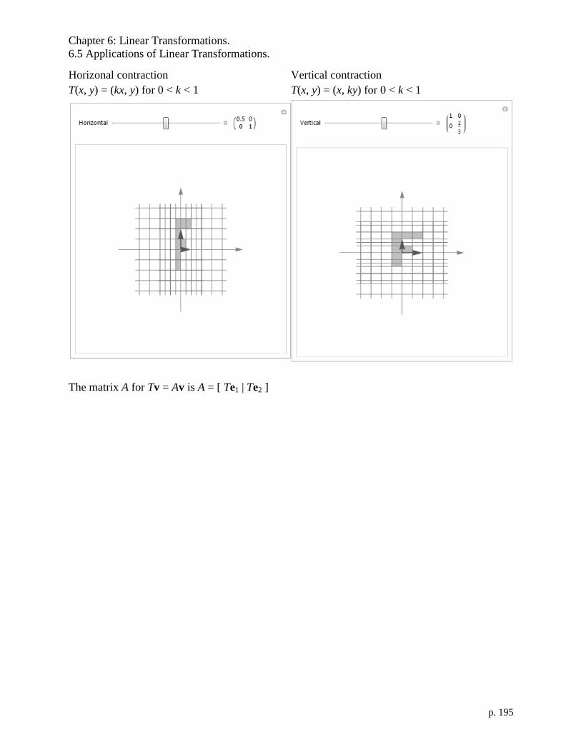
Chapter 6: Linear Transformations.
6.5 Applications of Linear Transformations.
p. 195
Horizonal contraction Vertical contraction
T(x, y) = (kx, y) for 0 < k < 1 T(x, y) = (x, ky) for 0 < k < 1
The matrix A for Tv = Av is A = [ Te1 | Te2 ]

Chapter 6: Linear Transformations.
6.5 Applications of Linear Transformations.
p. 196
Shears in R2.
Horizonal shear Vertical shear
T(x, y) = (–x, y) T(x, y) = (x, –y)
The matrix A for Tv = Av is A = [ Te1 | Te2 ]

Chapter 6: Linear Transformations.
6.5 Applications of Linear Transformations.
p. 197
Rotation in R2.
T(x, y) = (x cos( ) – y sin( ), x sin( ) + y cos( ))

Chapter 6: Linear Transformations.
6.5 Applications of Linear Transformations.
p. 198
Rotation in R3.
The matrix A for Tv = Av is A = [ Te1 | Te2 | Te3 ]
Rotation about x-axis by /6 rad = 30 counterclockwise (right-hand rule).

Chapter 6: Linear Transformations.
6.5 Applications of Linear Transformations.
p. 199
Rotation about y-axis by /6 rad = 30 Rotation about y-axis by /6 rad = 30
The matrix A for Tv = Av is A = [ Te1 | Te2 | Te3 ]


Chapter 7: Eigenvalues and Eigenvectors.
7.1 Eigenvalues and Eigenvectors.
p. 201
S*
Chapter 7: Eigenvalues and Eigenvectors.
7.1 Eigenvalues and Eigenvectors.
Objective: Prove properties of eigenvalues and eigenvectors.
Objective: Verify eigenvalues and corresponding eigenvectors.
Objective: Find eigenvalues and corresponding eigenspaces.
Objective: Use the characteristic equation to find eigenvalues and eigenvectors.
Objective: Use software to find eigenvalues and eigenvectors.
Recall the example A =
01
10 from Section 6.5. Then Ae1 =
01
10
0
1 =
1
0 = e2
and Ae2 =
01
10
1
0 =
0
1 = e1
Let x1 =
5.1
5.1. Then Ax1 =
01
10
5.1
5.1 =
5.1
5.1 = 1x1
Let x2 =
5.1
5.1. Then Ax2 =
01
10
5.1
5.1 =
5.1
5.1 = –1x2
Given square matrix A, if we have a nonzero vector x and a scalar (“lambda”) such that
Ax = x
then x is an eigenvector of A with the corresponding eigenvalue .
Example:
01
10 has eigenvectors x1 =
5.1
5.1, x2 =
5.1
5.1 with eigenvalues 1= 1, 2 = –1.
“Eigen” is German
for “particular.”

Chapter 7: Eigenvalues and Eigenvectors.
7.1 Eigenvalues and Eigenvectors.
p. 202
S*
S*
Example Show that
2
1 is an eigenvector of
60.030.0
05.065.0 , and find the corresponding
eigenvalue.
Solution:
Theorem 7.1: Eigenvectors of Form a Subspace
If A is an nn matrix with an eigenvalue , then the set of all eigenvectors of , together with the
zero vector
{x: x is an eigenvector of } {0} = {x: Ax = x}
is a subspace of Rn.
Proof:
{x: Ax = x} is not empty because it contains the zero vector.
{x: Ax = x} is closed under scalar multiplication because
for any vector x {x: Ax = x} and for any scalar c, A(cx) = c(Ax) = c(x) = (cx)
{x: Ax = x} is closed under addition because for any vectors x1, x2 {x: Ax = x},
A(x1 + x2) = Ax1 + Ax2 = x1 + x2 = (x1 + x2)
To find an eigenvalue of a matrix A, we start with the equation Ax = x.
Ax = x
Ax = Ix
0 = Ix – Ax
0 = (I – A)x
I – A is singular
det(I – A) = 0
Chapter 7: Eigenvalues and Eigenvectors.
7.1 Eigenvalues and Eigenvectors.
p. 203
S*
Theorem 7.2: Eigenvalues and Eigenvectors of a Matrix
Let A be an nn matrix.
1) An eigenvalue of A is a scalar such det(I – A) = 0.
2) The eigenvectors of A corresponding to are the nonzero solutions of (I – A)x = 0
i.e. the nullspace of I – A.
Proof:
A has an eigenvector x 0 with eigenvalue if and only if
if and only if A – I is singular (so its determinant is zero) and x is in the nullspace of A – I.
det(I – A) = 0 is called the characteristic equation of A. The characteristic polynomial
det(I – A) is an nth
-degree polynomial in .
The Fundamental Theorem of Algebra states that an nth
-degree polynomial has exactly n roots
(i.e. an nth
-degree polynomial equation has exactly n solutions). In other words, we will always
have
det(I – A) = ( – 1) ( – 2) … ( – n)
where the n constants 1, 2, …, n are the eigenvalues of A. Note that some i may be complex
or some i may be repeated, for example 1 = 2.
Example Find the eigenvalues and corresponding eigenvectors of A =
13
21.
Solution by hand: 0 = det(
Chapter 7: Eigenvalues and Eigenvectors.
7.1 Eigenvalues and Eigenvectors.
p. 204
so 1 =2 =
Eigenvector for 1 =
Eigenvector for 2 =
Example Find the eigenvalues and corresponding eigenvectors of A =
01
10.
Solution: 0 = det(
so 1 = 2 =
Chapter 7: Eigenvalues and Eigenvectors.
7.1 Eigenvalues and Eigenvectors.
p. 205
Eigenvector for 1 =
Eigenvector for 2 =
Example Find the eigenvalues and corresponding eigenvectors of A =
2.18.04.0
8.02.14.0
8.08.06.1
.
Solution: 0 = det(
so 1 = 2 = 3 =
Eigenvector for 1 =

Chapter 7: Eigenvalues and Eigenvectors.
7.1 Eigenvalues and Eigenvectors.
p. 206
Using rref we find which has a solution x =
E’vector for 2 = 3 =

Chapter 7: Eigenvalues and Eigenvectors.
7.1 Eigenvalues and Eigenvectors.
p. 207
Using rref we find which has solution
Note that this eigenvalue, which has multiplicity two, has two linearly independent
eigenvectors.
Example Find the eigenvalues and corresponding eigenvectors of A =
a
ba
0 where b 0.
Solution: 0 = det(
so 1 = 2 =
Eigenvector for 1 =
Eigenvector for 2 =
Note that this eigenvalue has multiplicity two but has only one linearly independent
eigenvector.
Using software to find eigenvalues and eigenvectors. Let A =
23
41 and B =
01
10.
TI-89: Use
MatrixeigVl(A)
and
MatrixeigVc(A)
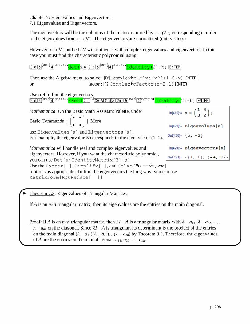
Chapter 7: Eigenvalues and Eigenvectors.
7.1 Eigenvalues and Eigenvectors.
p. 208
S*
The eigenvectors will be the columns of the matrix returned by eigVc, corresponding in order
to the eigenvalues from eigVl. The eigenvectors are normalized (unit vectors).
However, eigVl and eigV will not work with complex eigenvalues and eigenvectors. In this
case you must find the characteristic polynomial using
Matrixdet(x
Matrixidentity(2)-b)
Then use the Algebra menu to solve: ComplexcSolve(x^2+1=0,x)
or factor : ComplexcFactor(x^2+1)
Use rref to find the eigenvectors:
Matrixrref(
Matrixidentity(2)-b)
Mathematica: On the Basic Math Assistant Palette, under
Basic Commands |
| More
use Eigenvalues[a] and Eigenvectors[a].
For example, the eigenvalue 5 corresponds to the eigenvector (1, 1).
Mathematica will handle real and complex eigenvalues and
eigenvectors. However, if you want the characteristic polynomial,
you can use Det[x*IdentityMatrix[2]-a]
Use the Factor[ ], Simplify[ ], and Solve[lhs ==rhs,var]
funtions as appropriate. To find the eigenvectors the long way, you can use MatrixForm[RowReduce[ ]]
Theorem 7.3: Eigenvalues of Triangular Matrices
If A is an nn triangular matrix, then its eigenvalues are the entries on the main diagonal.
Proof: If A is an nn triangular matrix, then I – A is a triangular matrix with – a11, – a22, …,
– ann on the diagonal. Since I – A is triangular, its determinant is the product of the entries
on the main diagonal ( – a11)( – a22)…( – ann) by Theorem 3.2. Therefore, the eigenvalues
of A are the entries on the main diagonal: a11, a22, …, ann.

Chapter 7: Eigenvalues and Eigenvectors.
7.2 Diagonalization.
p. 209
S*
7.2 Diagonalization.
Objective: Prove properties of eigenvalues and eigenvectors.
Objective: Find the eigenvalues of similar matrices, determine whether a matrix is
diagonalizable, and find a matrix P such that P–1
AP is diagonal.
Objective: Find, for a linear transformation T: V V a basis B for V such that the matrix for T
relative to B is diagonal.
An nn matrix A is diagonalizable when there exists an invertible matrix P such that D = P–1
AP
is a diagonal matrix.
Recall from Section 6.4 that two square matrices A and B are similar if and only there is an
invertible matrix P such that B = P–1
AP. So we can also say that A is diagonalizable when it it
similar to a diagonal matrix D.
Theorem 7.4: Similar Matrices Have the Same Eigenvalues
If A and B are similar nn matrices, then they have the same eigenvalues.
Proof: Because A and B are similar, there exists an invertible matrix P such that B = P–1
AP, so
|I – B| = | P–1
IP – P–1
AP | = |P–1
(I – A)P| = |P–1
| |(I – A)| |P| =||
1
P |(I – A)| |P| = |(I – A)|
Since A and B have the same characteristic polynomial, they must have the same eigenvalues.
Theorem 7.5: Condition for Diagonalization
An nn matrix A is diagonalizable if and only if it has n linearly independent eigenvectors.
Proof:
First, assume A is diagonalizable. Then there exists an invertible matrix P such that D = P–1
AP
is a diagonal matrix. Then PD = AP. Let the column vectors of P be p1, p2, …, pn and the main
diagonal entries of D be 1, 2, …, n.
Now PD = [ p1 | p2 | … | pn ]
n
000
00
00
2
1
= [ 1p1 | 2p2 | … | npn ]
and AP = A[ p1 | p2 | … | pn ] = [ Ap1 | Ap2 | … | Apn ]

Chapter 7: Eigenvalues and Eigenvectors.
7.2 Diagonalization.
p. 210
Since PD = AP, we have Api = ipi for each of the n column vectors of P. Since P is invertible,
the n column vectors are also linearly independent. So A has n linearly independent
eigenvectors.
Conversely, assume A has n linearly independent eigenvectors p1, p2, …, pn with
corresponding eigenvalues 1, 2, …, n. Let P be the matrix whose columns are the n
eigenvectors: P = [ p1 | p2 | … | pn ]. Then
AP = A[ p1 | p2 | … | pn ] = [ Ap1 | Ap2 | … | Apn ] = [ 1p1 | 2p2 | … | npn ]
= [ p1 | p2 | … | pn ]
n
000
00
00
2
1
Thus, AP = PD, where D =
n
000
00
00
2
1
is a diagonal matrix. Since the pi are linearly
independent, P is invertible, so D = P–1
AP and A is diagonalizable.
Example Diagonalize A =
020
200
123
by finding an invertible matrix P and a diagonal matrix D
such that D = P–1
AP. Use the characteristic polynomial to find the eigenvalues and the reduced
row-echechelon function of your software to find the eigenvectors.
Solution: 0 = det(
=
so 1 = 2 = 3 =

Chapter 7: Eigenvalues and Eigenvectors.
7.2 Diagonalization.
p. 211
Eigenvector for 1 =
Eigenvector for 2 =
Eigenvector for 3 =
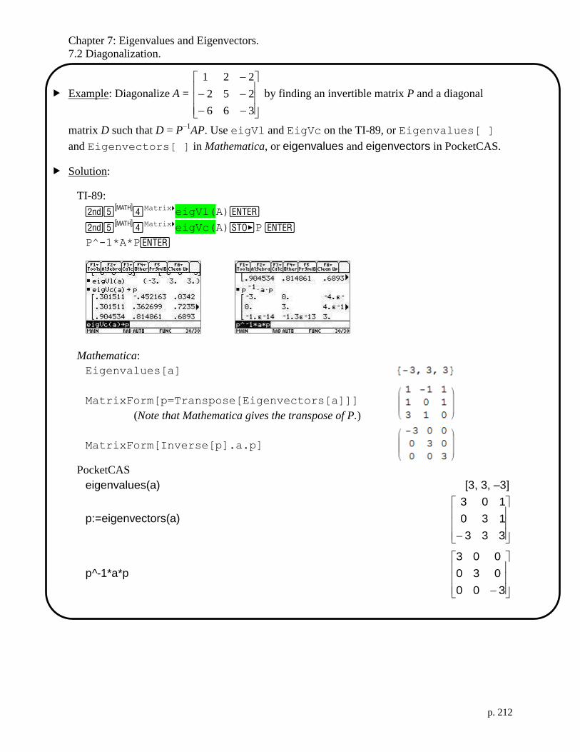
Chapter 7: Eigenvalues and Eigenvectors.
7.2 Diagonalization.
p. 212
S*
Example: Diagonalize A =
366
252
221
by finding an invertible matrix P and a diagonal
matrix D such that D = P–1
AP. Use eigVl and EigVc on the TI-89, or Eigenvalues[ ]
and Eigenvectors[ ] in Mathematica, or eigenvalues and eigenvectors in PocketCAS.
Solution:
TI-89:
MatrixeigVl(A)
MatrixeigVc(A)P
P^-1*A*P
Mathematica:
Eigenvalues[a]
MatrixForm[p=Transpose[Eigenvectors[a]]]
(Note that Mathematica gives the transpose of P.)
MatrixForm[Inverse[p].a.p]
PocketCAS
eigenvalues(a) [3, 3, –3]
p:=eigenvectors(a)
333
130
103
p^-1*a*p
300
030
003

Chapter 7: Eigenvalues and Eigenvectors.
7.2 Diagonalization.
p. 213
Example: Try to diagonalize A =
201
121
001
Use eigVl and EigVc on the TI-89, or
Eigenvalues[ ] and Eigenvectors[ ] in Mathematica, or eigenvalues and
eigenvectors in PocketCAS.
Solution:
TI-89:
MatrixeigVl(A)
MatrixeigVc(A)P
P^(-1)*A*P Error: Singular Matrix
Mathematica:
Eigenvalues[a]
MatrixForm[p=Transpose[Eigenvectors[a]]]
(Note that Mathematica gives the transpose of P.)
MatrixForm[Inverse[p].a.p]
PocketCAS
eigenvalues(a) [2, 2, 1]
p:=eigenvectors(a) Not diagonalizable at eigenvalue 2


Chapter 7: Eigenvalues and Eigenvectors.
7.3 Symmetric Matrices and Orthogonal Diagonalization.
p. 215
S*
S*
7.3 Symmetric Matrices and Orthogonal Diagonalization.
Objective: Recognize, and apply properties of, symmetric matrices.
Objective: Recognize, and apply properties of, orthogonal matrices.
Objective: Find an orthogonal matrix P that orthogonally diagonalizes a symmetric matrix A.
A square matrix A is symmetric when A = AT.
Theorem 7.7: Properties of Symmetric Matrices
If A is a symmetric nn matrix, then
1) A is diagonalizable.
2) All eigenvalues of A are real.
3) If is an eigenvalue of A with multiplicity k, then has k linearly independent eigenvectors.
That is, the eigenspace of has dimension k.
The proof will be deferred until Ch. 8.5
Theorem 7.9: Property of Symmetric Matrices
Let A be an nn symmetric matrix. if 1 and 2 are distinct eigenvalues of A, then their
corresponding eignevectors x1 and x2 are orthogonal.
Proof:
Let 1 and 2 are distinct eigenvalues of A with corresponding eignevectors x1 and x2, so
Ax1 = 1x1 and Ax2 = 2x2. Recall that we can write x1•x2 = x1Tx2. Then
1 (x1•x2) = (1x1)•x2
= (Ax1)•x2
= 2(x1•x2)
Therefore, (1 – 2)(x1•x2) = 0. Since 1 – 2 0, we must have x1•x2 = 0 so x1 and x2 are
orthogonal.

Chapter 7: Eigenvalues and Eigenvectors.
7.3 Symmetric Matrices and Orthogonal Diagonalization.
p. 216
Example: Find the eigenvalues and eigenvectors of
011
101
110
. Are the eigenvalues real? What
are the dimensions of the eigenspaces? Find the angles between the eigenvectors.
Solution:
0 = det(
100
010
001
–
011
101
110
)
(using the calculator to take the determinant and factor it.)
1 = 2, 2 = –1, 3 = –1. All eigenvalues are real.
Solve (1I –
011
101
110
)x1 = 0 using rref.
Write x1=
3
2
1
. 3 = t is a free variable. We solve for 1 = t and 1 = t.
The solution is
t
t
t
= t
1
1
1
so x1 =
1
1
1
.
The eigenspace of = 2 (multiplicity = 1) is one-dimesional.
Solve (2I –
011
101
110
)x2 = 0 and
Solve (3I –
011
101
110
)x3 = 0 using rref. (Note 2 = 3.)
2 = s and 3 = t are free variables. We solve for 1 = –s – t.
The solution is
t
s
ts
= s
0
1
1
+ t
1
0
1
so x2 =
0
1
1
and x3 =
1
0
1
.
is the
Greek letter
xi
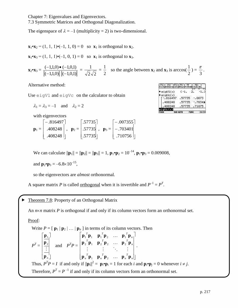
Chapter 7: Eigenvalues and Eigenvectors.
7.3 Symmetric Matrices and Orthogonal Diagonalization.
p. 217
S*
The eigenspace of = –1 (multiplicity = 2) is two-dimensional.
x1•x2 = (1, 1, 1)•(–1, 1, 0) = 0 so x1 is orthogonal to x2.
x1•x3 = (1, 1, 1)•(–1, 0, 1) = 0 so x1 is orthogonal to x3.
x2•x3 = )1,0,1()0,1,1(
)1,0,1()0,1,1(
=
22
1 =
2
1 so the angle between x2 and x3 is arccos(
2
1) =
3
.
Alternative method:
Use eigVl and eigVc on the calculator to obtain
1 = 3 = –1 and 2 = 2
with eigenvectors
p1 =
408248.
408248.
816497.
, p2 =
57735.
57735.
57735.
, p3 =
710756.
703401.
007355.
We can calculate ||p1|| = ||p2|| = ||p3|| = 1, p1•p2 = 10–14
, p1•p3 = 0.009008,
and p2•p3 = –6.810–15
,
so the eigenvectors are almost orthonormal.
A square matrix P is called orthogonal when it is invertible and P–1
= PT.
Theorem 7.8: Property of an Orthogonal Matrix
An nn matrix P is orthogonal if and only if its column vectors form an orthonormal set.
Proof:
Write P = [ p1 | p2 | … | pn ] in terms of its column vectors. Then
PT =
np
p
p
2
1
and PTP =
n
T
n
T
n
T
n
n
TTT
n
TTT
pppppp
pppppp
pppppp
21
22212
12111
.
Thus, PTP = I if and only if ||pi||
2 = pi•pi = 1 for each i and pi•pj = 0 whenever i j.
Therefore, PT = P
–1 if and only if its column vectors form an orthonormal set.

Chapter 7: Eigenvalues and Eigenvectors.
7.3 Symmetric Matrices and Orthogonal Diagonalization.
p. 218
S*
Because of this theorem, it would have been better if orthogonal matrices had been called
“orthonormal matrices.” but we are stuck with the name “orthogonal.”
Theorem 7.10: Fundamental Property of an Symmetric Matrices
Let A be a real nn matrix. Then A is orthogonally diagonalizable and has real eigenvalues if and
only if A is symmetric.
Proof:
Suppose A is orthogonally diagonalizable and real, so there exists a real, orthogonal matrix P
such that D = P –1
AP is diagonal and real. Then
= PDP –1
= PDPT
so
AT = (PDP
T)
T
= (PT)TD
TP
T
= PDPT
= A
Conversely, Theorems 7.7 and 7.9 together tell us that all symmetric matrices are orthogonally
diagonalizable with real eigenvalues.
An nn symmentric matrix has n eigenvalues, counting multiplicity. Because the dimension
of each eigenspace equals the multiplicity of the corresponding eigenvalue, we have n
linearly independent eigenvectors, so the matrix is diagonalizable (Theorem 7.5).
Eigenvectors with different eigenvalues are orthogonal. Within each eigenspace, we can use
the Gram-Schmidt process to find orthonormal eigenvectors. The set of all of the
orthonormal eigenvectors from all of the eigenspaces make up the columns of an orthogonal
matrix P, such that
D = P –1
AP
is diagonal.
Example (continued): Diagonalize
011
101
110
using…
1) the characteristic equation and rref
2) eigVl and eigVc on the TI-89
3) Eigenvalues[ ] and Eigenvectors[ ] in Mathematica
4) eigenvalues and eigenvectors in PocketCAS
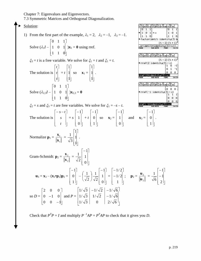
Chapter 7: Eigenvalues and Eigenvectors.
7.3 Symmetric Matrices and Orthogonal Diagonalization.
p. 219
Solution:
1) From the first part of the example, 1 = 2, 2 = –1, 3 = –1.
Solve (1I –
011
101
110
)x1 = 0 using rref.
3 = t is a free variable. We solve for 1 = t and 1 = t.
The solution is
t
t
t
= t
1
1
1
so x1 =
1
1
1
.
Solve (2,3I –
011
101
110
)x2,3 = 0
2 = s and 3 = t are free variables. We solve for 1 = –s – t.
The solution is
t
s
ts
= s
0
1
1
+ t
1
0
1
so x2 =
0
1
1
and x3 =
1
0
1
.
Normalize p1 = 1
1
x
x =
1
1
1
3
1.
Gram-Schmidt: p2 = 2
2
x
x =
0
1
1
2
1
u3 = x3 – (x3•p2)p2 =
1
0
1
–
2
1
0
1
1
2
1 =
1
2/1
2/1
; p2 = 2
2
u
u =
2
1
1
6
1
so D =
100
010
002
and P =
6/203/1
6/12/13/1
6/12/13/1
Check that PTP = I and multiply P
–1AP = P
TAP to check that it gives you D.

Chapter 7: Eigenvalues and Eigenvectors.
7.3 Symmetric Matrices and Orthogonal Diagonalization.
p. 220
2) TI-89: Use eigVl and eigVc to obtain
D =
100
020
001
and P =
710756.57735.408248.
703401.57735.408248.
077355.57735.816497.
Check PTP =
.115E8.6009008.
15E8.6.114E.1
009008.14E.1.1
so P is almost orthogonal.
By looking at the ratios between components, it appears that
p1 = unitV([-2,1,1]) = 6/66/63/6
p2 = unitV([1,1,1]) = 3/33/33/3
p3 = unitV([0,-1,1]) = 2/22/20
Try a new P =
2/23/36/6
2/23/36/6
03/33/6
p gives
707107.57735.408248.
707107.57735.408248.
057735.816497.
Check that PTP = I and multiply P
–1AP = P
TAP to check that it gives you D.
3) Mathematica: Eigenvalues[a] yields {2,-1,-1} so D =
100
010
002
Eigenvalues[a] gives {{1,1,1},{-1,0,1},{-1,1,0}} so
x1 =
1
1
1
, x2 =
1
0
1
, x3 =
0
1
1
Warning: MatrixForm[Eigenvalues[a]] gives
which has the eigenvectors in the rows (instead of in
the columns)!

Chapter 7: Eigenvalues and Eigenvectors.
7.3 Symmetric Matrices and Orthogonal Diagonalization.
p. 221
Orthogonalize[Eigenvalues[a]] gives the orthonormal basis
so P =
6/12/13/1
3/203/1
6/12/13/1
Warning: MatrixForm[Orthogonalize[Eigenvalues[a]]] gives PT, not P!
Check that PTP = I and multiply P
–1AP = P
TAP to check that it gives you D.
4) PocketCAS: Computing M T
M shows in the off-diagonal
elements that the vectors are orthogonal,
and the diagonal elements give the norm
squared of each vector.
so D =
100
010
002
gramschmidt( ) will construct an eigenvectors( ) orthonormal basis from the rows of a matrix,
gives orthogonal, so use gramschmidt(transpose(p)) to
but unnormalized obtain PT.
eigenvectors.
so P =
6/12/13/1
6/203/1
6/12/13/1
Check that PTP = I and multiply P
–1AP = P
TAP to check that it gives you D.

Chapter 7: Eigenvalues and Eigenvectors.
7.3 Symmetric Matrices and Orthogonal Diagonalization.
p. 222
Example: Diagonalize
444
422
422
.

Chapter 7: Eigenvalues and Eigenvectors.
8.5 Unitary and Hermitian Matrices.
p. 223
8.5 Unitary and Hermitian Matrices.
Objective: Find the conjugate transpose (Hermitian conjugate) of a complex matrix A.
Objective: Determine if a matrix A is unitary.
Objective: Find the eigenvalues and eigenvectors of a Hermitian matrix, and diagonalize a
Hemitian matrix.
In order to prove the theorems in Section 7.4 about real symmetric matrices, we must consider
complex “Hermitian” matices.
The conjugate transpose (or Hermitian conjugate) of a complex matrix A, denoted by A† or A
H or
A*, is given by A† = (𝐴 ̅)𝑇 = 𝐴𝑇̅̅̅̅ . That is, Take the complex conjugate of each of entry of A, and
transpose the matrix.
Notice that if A is real (all entries are real), then A† = A
T.
A is Hermitian if and only if A† = A. Notice that if A is real, then Hermitian is the same as
symmetric.
To take the Hermitian conjugate A† on the TI-89, use a
Matrix
T
To take the Hermitian conjugate A† in Mathematica, use act
To take the Hermitian conjugate A† in PocketCAS, use trn(a)
A is unitary if and only if A† = A
–1. Notice that if A is real, then unitary is the same as orthogonal.
Example: Classify the following matrices as Hermitian, unitary, both, or neither.
1) A =
0
0
i
i: A
† =
0
0
i
i. A
† = A so A is Hermitian. AA
† = I so A is also unitary.
2) B = : B† = . B
† B so B is not Hermitian.
BB† = I so B is unitary.
3) C =
523
234
7
1
i
i: C
† =
523
234
7
1
i
i. C
† = C so C is Hermitian.
CC† = I so C is not unitary.

Chapter 7: Eigenvalues and Eigenvectors.
8.5 Unitary and Hermitian Matrices.
p. 224
S*
4) D =
i0
01: D
† =
i0
01. D
† D so D is not Hermitian. D
†D =
10
01 I so D is not
unitary.
Theorem 8.8: Properties of the Hermitian Conjugate (Complex Transpose)
If A, B, and C complex matrices with dimensions mn, mn, and np respectively, and k is a
complex number, then the following properties are true.
1) (A†)† = A
2) (A + B)† = A
† + B
†
3) (kA)† = �̅�A
†
4) (AC)† = C
†A
†
Theorem 8.9: Unitary Matrices
An nn complex matrix U is unitary if and only if its row vectors form an orthonormal set in Cn
using the Euclidean inner product.
Proof:
Recall that the Euclidean inner product of u and v in Cn is given by
u•v = 𝑢1𝑣1̅̅ ̅ + 𝑢2𝑣2̅̅ ̅ + ⋯ + 𝑢𝑛𝑣𝑛̅̅ ̅
Note that if we write u and v as row vectors, then u•v = u v†
||u|| = uu and u is orthogonal to v if and only if u•v = 0.
Write A =
nu
u
u
2
1
in terms of its row vectors. Then
AT = [ u1
† | u 2
† | … | un
† ] and AA
† =
nnnn
n
n
uuuuuu
uuuuuu
uuuuuu
21
22212
12111
.
Thus, AA† = I if and only if ||ui||
2 = ui•ui = 1 for each i and ui•uj = 0 whenever i j.
Therefore, A† = A
–1 if and only if its row vectors form an orthonormal set.
Theorem 8.9.1: A is unitary if and only if A† is unitary.

Chapter 7: Eigenvalues and Eigenvectors.
8.5 Unitary and Hermitian Matrices.
p. 225
Corollary 8.9.2: Unitary Matrices
An nn complex matrix A is unitary if and only if its column vectors form an orthonormal set in
Cn using the Euclidean inner product.
Theorem 8.10: The Eigenvalues of a Hermitian Matrix
If H is a Hermitian matrix, then its eigenvalues are real.
Proof:
Let be an eigenvalue of H and let v 0 be its corresponding eigenvalue, so Hv = v.
Then (v†Hv)
† = v
†H
†(v
†)† = v
†Hv
Now v†Hv = v
†(Hv) = v
†(v) = (v
†v) = ||v||
2
So (v†Hv)
† = ‖𝐯‖2̅̅ ̅̅ ̅̅ ̅̅ = ̅||v||
2 because ||v|| is real.
Since ||v|| 0 and ||v||2 = ̅||v||
2, must be real.


420 Chapter 8 Complex Vector Spaces
8.5 Unitary and Hermitian Matrices
Find the conjugate transpose of a complex matrix
Determine if a matrix is unitary.
Find the eigenvalues and eigenvectors of a Hermitian matrix, anddiagonalize a Hermitian matrix.
CONJUGATE TRANSPOSE OF A MATRIX
Problems involving diagonalization of complex matrices and the associated eigenvalueproblems require the concepts of unitary and Hermitian matrices. These matricesroughly correspond to orthogonal and symmetric real matrices. In order to define unitary and Hermitian matrices, the concept of the conjugate transpose of a complexmatrix must first be introduced.
Note that if is a matrix with real entries, then * . To find the conjugatetranspose of a matrix, first calculate the complex conjugate of each entry and then takethe transpose of the matrix, as shown in the following example.
Finding the Conjugate Transpose
of a Complex Matrix
Determine * for the matrix
SOLUTION
Several properties of the conjugate transpose of a matrix are listed in the followingtheorem. The proofs of these properties are straightforward and are left for you to supply in Exercises 47–50.
A* � AT � �3 � 7i0
�2i4 � i�
A � �3 � 7i2i
04 � i� � �3 � 7i
�2i0
4 � i�
A � �3 � 7i2i
04 � i�.
A
� ATAA
A
A.A*
Definition of the Conjugate Transpose of a Complex Matrix
The conjugate transpose of a complex matrix denoted by *, is given by
*
where the entries of are the complex conjugates of the corresponding entriesof A.
A
� A TA
AA,
THEOREM 8.8 Properties of the Conjugate Transpose
If and are complex matrices and is a complex number, then the followingproperties are true.
1. 2.3. 4. �AB�* � B*A*�kA�* � kA*
�A � B�* � A* � B*�A*�* � A
kBA
9781133110873_0805.qxp 3/10/12 6:55 AM Page 420

UNITARY MATRICES
Recall that a real matrix is orthogonal if and only if In the complex system, matrices having the property that * are more useful, and such matricesare called unitary.
A Unitary Matrix
Show that the matrix is unitary.
SOLUTION
Begin by finding the product *.
Because
it follows that So, is a unitary matrix.
Recall from Section 7.3 that a real matrix is orthogonal if and only if its row (or column) vectors form an orthonormal set. For complex matrices, this property characterizes matrices that are unitary. Note that a set of vectors
in (a complex Euclidean space) is called orthonormal when the statements below are true.
1.
2.
The proof of the next theorem is similar to the proof of Theorem 7.8 presented inSection 7.3.
i � jvi � vj � 0,
�vi� � 1, i � 1, 2, . . . , m
Cn
�v1, v2, . . . , vm�
AA* � A�1.
AA* � �10
01� � I2
� �10
01�
�14�
40
04�
AA* �12�
1 � i1 � i
1 � i1 � i�
12 �
1 � i1 � i
1 � i1 � i�
AA
A �12 �
1 � i1 � i
1 � i1 � i�A
A�1 � AA�1 � AT.A
8.5 Unitary and Hermitian Matrices 421
Definition of Unitary Matrix
A complex matrix is unitary when
A�1 � A*.
A
THEOREM 8.9 Unitary Matrices
An complex matrix is unitary if and only if its row (or column) vectorsform an orthonormal set in Cn.
An � n
9781133110873_0805.qxp 3/10/12 6:55 AM Page 421
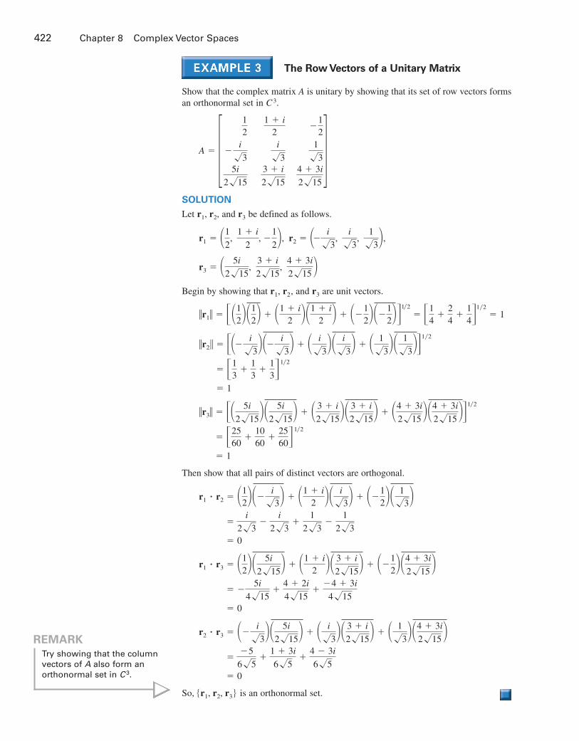
The Row Vectors of a Unitary Matrix
Show that the complex matrix is unitary by showing that its set of row vectors formsan orthonormal set in
SOLUTION
Let and be defined as follows.
Begin by showing that and are unit vectors.
Then show that all pairs of distinct vectors are orthogonal.
So, is an orthonormal set.�r1, r2, r3�
� 0
��5
65�
1 � 3i
65�
4 � 3i
65
r2 � r3 � �i
3�5i
215� � i3�
3 � i
215� � 13�
4 � 3i
215 � � 0
� �5i
415�
4 � 2i
415�
�4 � 3i
415
r1 � r3 � 12�
5i
215� � 1 � i2 � 3 � i
215� � �12�
4 � 3i
215 � � 0
�i
23�
i
23�
1
23�
1
23
r1 � r2 � 12��
i3� � 1 � i
2 � i3� � �
12�
13�
� 1
� �2560
�1060
�2560�
1�2
�r3� � � 5i
215�5i
215� � 3 � i
215�3 � i
215� � 4 � 3i
215 �4 � 3i
215 ��1�2
� 1
� �13
�13
�13�
1�2
�r2� � �� i3��
i3� � i
3�i
3� � 13�
13��
1�2
�r1� � �12�
12� � 1 � i
2 �1 � i2 � � �
12��
12��
1�2
� �14
�24
�14�
1�2� 1
r3r2,r1,
r3 � 5i
215,
3 � i
215,
4 � 3i
215 �
r2 � � i3
, i
3,
13�,r1 � 1
2,
1 � i
2, �
1
2�,
r3r1, r2,
A � �12
�i
35i
215
1 � i2i
33 � i
215
�12
13
4 � 3i
215
�C3.
A
422 Chapter 8 Complex Vector Spaces
REMARK
Try showing that the columnvectors of also form anorthonormal set in C3.
A
9781133110873_0805.qxp 3/10/12 6:55 AM Page 422

HERMITIAN MATRICES
A real matrix is symmetric when it is equal to its own transpose. In the complex system, the more useful type of matrix is one that is equal to its own conjugatetranspose. Such a matrix is called Hermitian after the French mathematician CharlesHermite (1822–1901).
As with symmetric matrices, you can recognize Hermitian matrices by inspection.To see this, consider the matrix
The conjugate transpose of has the form
If is Hermitian, then So, must be of the form
Similar results can be obtained for Hermitian matrices of order In other words,a square matrix is Hermitian if and only if the following two conditions are met.
1. The entries on the main diagonal of are real.
2. The entry in the th row and the th column is the complex conjugate of theentry in the th row and the th column.
Hermitian Matrices
Which matrices are Hermitian?
a. b.
c. d.
SOLUTION
a. This matrix is not Hermitian because it has an imaginary entry on its main diagonal.
b. This matrix is symmetric but not Hermitian because the entry in the first row andsecond column is not the complex conjugate of the entry in the second row and firstcolumn.
c. This matrix is Hermitian.
d. This matrix is Hermitian because all real symmetric matrices are Hermitian.
��1
23
20
�1
3�1
4��3
2 � i3i
2 � i0
1 � i
�3i1 � i
0�� 0
3 � 2i3 � 2i
4�� 1
3 � i
3 � i
i �
ijaji
jiaij
A
An � n.
A � � a1
b1 � b2ib1 � b2i
d1�.
AA � A*.A
� �a1 � a2ib1 � b2i
c1 � c2id1 � d2i
�.
� �a1 � a2i
b1 � b2i
c1 � c2i
d1 � d2i� A* � AT
A
A � �a1 � a2ic1 � c2i
b1 � b2id1 � d2i
�A.2 � 2
8.5 Unitary and Hermitian Matrices 423
Definition of a Hermitian Matrix
A square matrix is Hermitian when
A � A*.
A
9781133110873_0805.qxp 3/10/12 6:55 AM Page 423

One of the most important characteristics of Hermitian matrices is that their eigenvalues are real. This is formally stated in the next theorem.
PROOF
Let be an eigenvalue of and let
be its corresponding eigenvector. If both sides of the equation are multipliedby the row vector then
Furthermore, because
it follows that * is a Hermitian matrix. This implies that * is a real number, so is real.
To find the eigenvalues of complex matrices, follow the same procedure as for realmatrices.
Finding the Eigenvalues of a Hermitian Matrix
Find the eigenvalues of the matrix
SOLUTION
The characteristic polynomial of is
So, the characteristic equation is and the eigenvalues of are and �2.�1, 6,
A�� � 1��� � 6��� � 2� � 0,
� �� � 1��� � 6��� � 2�. � �3 � 3�2 � 16� � 12
� ��3 � 3�2 � 2� � 6� � �5� � 9 � 3i� � �3i � 9 � 9��� 3i �1 � 3i� � 3�i�
� �� � 3���2 � 2� � ��2 � i� ��2 � i�� � �3i � 3��
��I � A� � � � � 3�2 � i
�3i
�2 � i�
�1 � i
3i�1 � i
� �A
A � �3
2 � i3i
2 � i0
1 � i
�3i1 � i
0�A.
�Avv1 � 1Avv
�v*Av�* � v*A*�v*�* � v*Av
v*Av � v*��v� � ��v*v� � ��a12 � b1
2 � a22 � b2
2 � . . . � an2 � bn
2�.
v*,Av � �v
v � �a1 � b1i
a2 � b2i
..
.
an � bni�
A�
424 Chapter 8 Complex Vector Spaces
THEOREM 8.10 The Eigenvalues of a Hermitian Matrix
If is a Hermitian matrix, then its eigenvalues are real numbers.A
REMARK
Note that this theorem impliesthat the eigenvalues of a realsymmetric matrix are real, asstated in Theorem 7.7.
9781133110873_0805.qxp 3/10/12 6:55 AM Page 424
To find the eigenvectors of a complex matrix, use a procedure similar to that usedfor a real matrix. For instance, in Example 5, to find the eigenvector corresponding tothe eigenvalue substitute the value for into the equation
to obtain
Solve this equation using Gauss-Jordan elimination, or a graphing utility or softwareprogram, to obtain the eigenvector corresponding to which is shown below.
Eigenvectors for and can be found in a similar manner. They are
and respectively.�1 � 3i
�2 � i
5�,�
1 � 21i
6 � 9i
13�
�3 � �2�2 � 6
v1 � ��1
1 � 2i
1�
�1 � �1,
��4
�2 � i�3i
�2 � i�1
�1 � i
3i�1 � i
�1��v1
v2
v3� � �
000�.
�� � 3
�2 � i�3i
�2 � i�
�1 � i
3i�1 � i
���
v1
v2
v3� � �
000�
�� � �1,
8.5 Unitary and Hermitian Matrices 425
LINEAR ALGEBRA APPLIED
Quantum mechanics had its start in the early 20th centuryas scientists began to study subatomic particles and light.Collecting data on energy levels of atoms, and the rates oftransition between levels, they found that atoms could beinduced to more excited states by the absorption of light.
German physicist Werner Heisenburg (1901–1976) laid amathematical foundation for quantum mechanics usingmatrices. Studying the dispersion of light, he used vectors torepresent energy levels of states and Hermitian matrices torepresent “observables” such as momentum, position, andacceleration. He noticed that a measurement yields preciselyone real value and leaves the system in precisely one of a setof mutually exclusive (orthogonal) states. So, the eigenvaluesare the possible values that can result from a measurementof an observable, and the eigenvectors are the correspondingstates of the system following the measurement.
Let matrix be a diagonal Hermitian matrix that representsan observable. Then consider a physical system whosestate is represented by the column vector To measure thevalue of the observable in the system of state you canfind the product
Because is Hermitian and its values along the diagonalare real, is a real number. It represents the average of the values given by measuring the observable on asystem in the state a large number of times.u
Au*Au
A
� �u1u1�a11 � �u2u2�a22 � �u3u3�a33.
u*Au � u1 u2 u3��a11
00
0a22
0
00
a33��
u1
u2
u3�
u,Au.
A
TECHNOLOGY
Some graphing utilities andsoftware programs have built-inprograms for finding the eigenvalues and correspondingeigenvectors of complex matrices.
Jezper/Shutterstock.com
9781133110873_0805.qxp 3/10/12 6:55 AM Page 425

426 Chapter 8 Complex Vector Spaces
Just as real symmetric matrices are orthogonally diagonalizable, Hermitian matrices are unitarily diagonalizable. A square matrix is unitarily diagonalizablewhen there exists a unitary matrix such that
is a diagonal matrix. Because is unitary, *, so an equivalent statement is that is unitarily diagonalizable when there exists a unitary matrix such that *is a diagonal matrix. The next theorem states that Hermitian matrices are unitarily diagonalizable.
PROOF
To prove part 1, let and be two eigenvectors corresponding to the distinct (andreal) eigenvalues and Because and you have the equations shown below for the matrix product *
* *A* * * *
* * * *
So,
because
and this shows that and are orthogonal. Part 2 of Theorem 8.11 is often called theSpectral Theorem, and its proof is left to you.
The Eigenvectors of a Hermitian Matrix
The eigenvectors of the Hermitian matrix shown in Example 5 are mutually orthogonalbecause the eigenvalues are distinct. Verify this by calculating the Euclidean inner products and For example,
The other two inner products and can be shown to equal zero in a similar manner.
The three eigenvectors in Example 6 are mutually orthogonal because they correspond to distinct eigenvalues of the Hermitian matrix . Two or more eigenvectorscorresponding to the same eigenvalue may not be orthogonal. Once any set of linearlyindependent eigenvectors is obtained for an eigenvalue, however, the Gram-Schmidtorthonormalization process can be used to find an orthogonal set.
A
v2 � v3v1 � v3
� 0.
� �1 � 21i � 6 � 9i � 12i � 18 � 13
� ��1��1 � 21i� � �1 � 2i��6 � 9i� � 13
v1 � v2 � ��1��1 � 21i� � �1 � 2i��6 � 9i� � �1��13�
v2 � v3.v1 � v3,v1 � v2,
v2v1
�1� �2 v1*v2 � 0
��2 � �1�v1*v2 � 0
�2v1*v2 � �1v1*v2 � 0
v2�1v2 � �1v1v2 � v1v2 � ��1v1��Av1�v2�2v2 � �2v1Av2 � v1v2 � v1v2 � v1�Av1�
v2.�Av1�Av2 � �2v2,Av1 � �1v1�2.�1
v2v1
APPPAP�1 � PP
P�1AP
PA
THEOREM 8.11 Hermitian Matrices and Diagonalization
If is an Hermitian matrix, then
1. eigenvectors corresponding to distinct eigenvalues are orthogonal.2. is unitarily diagonalizable.A
n � nA
9781133110873_0805.qxp 3/10/12 6:55 AM Page 426
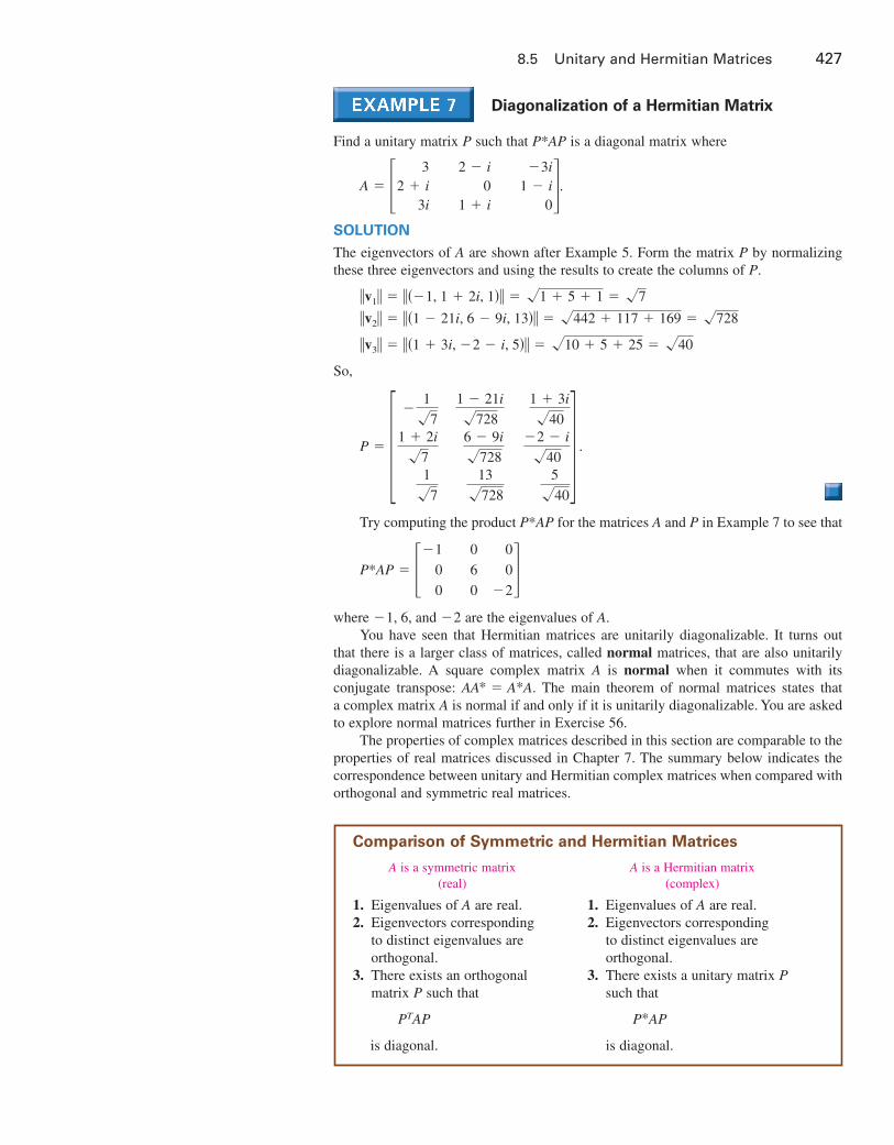
Diagonalization of a Hermitian Matrix
Find a unitary matrix such that * is a diagonal matrix where
SOLUTION
The eigenvectors of are shown after Example 5. Form the matrix by normalizingthese three eigenvectors and using the results to create the columns of
So,
Try computing the product * for the matrices and in Example 7 to see that
*
where and are the eigenvalues of You have seen that Hermitian matrices are unitarily diagonalizable. It turns out
that there is a larger class of matrices, called normal matrices, that are also unitarilydiagonalizable. A square complex matrix is normal when it commutes with its conjugate transpose: The main theorem of normal matrices states that a complex matrix is normal if and only if it is unitarily diagonalizable. You are askedto explore normal matrices further in Exercise 56.
The properties of complex matrices described in this section are comparable to theproperties of real matrices discussed in Chapter 7. The summary below indicates thecorrespondence between unitary and Hermitian complex matrices when compared withorthogonal and symmetric real matrices.
AAA* � A*A.
A
A.�2�1, 6,
AP � ��1
0
0
0
6
0
0
0
�2�P
PAAPP
P � ��
17
1 � 2i7
17
1 � 21i7286 � 9i728
13728
1 � 3i40
�2 � i40
540
� .
�v3� � ��1 � 3i, �2 � i, 5�� � 10 � 5 � 25 � 40
�v2� � ��1 � 21i, 6 � 9i, 13�� � 442 � 117 � 169 � 728
�v1� � ���1, 1 � 2i, 1�� � 1 � 5 � 1 � 7
P.PA
A � �3
2 � i3i
2 � i0
1 � i
�3i1 � i
0�.
APPP
8.5 Unitary and Hermitian Matrices 427
Comparison of Symmetric and Hermitian Matrices
A is a symmetric matrix A is a Hermitian matrix(real) (complex)
1. Eigenvalues of are real. 1. Eigenvalues of are real.2. Eigenvectors corresponding 2. Eigenvectors corresponding
to distinct eigenvalues are to distinct eigenvalues are orthogonal. orthogonal.
3. There exists an orthogonal 3. There exists a unitary matrix matrix such that such that
is diagonal. is diagonal.
P*APPTAP
PP
AA
9781133110873_0805.qxp 3/10/12 6:55 AM Page 427

428 Chapter 8 Complex Vector Spaces
8.5 Exercises
Finding the Conjugate Transpose In Exercises 1–4,determine the conjugate transpose of the matrix.
1. 2.
3. 4.
Finding the Conjugate Transpose In Exercises 5 and6, use a software program or graphing utility to find theconjugate transpose of the matrix.
5.
6.
Non-Unitary Matrices In Exercises 7–10, explain whythe matrix is not unitary.
7. 8.
9.
10.
Identifying Unitary Matrices In Exercises 11–16,determine whether is unitary by calculating *.
11. 12.
13. 14.
15.
16.
Row Vectors of a Unitary Matrix In Exercises 17–20,(a) verify that is unitary by showing that its rows areorthonormal, and (b) determine the inverse of
17. 18.
19.
20.
Identifying Hermitian Matrices In Exercises 21–26,determine whether the matrix is Hermitian.
21. 22.
23. 24.
25.
26.
Finding Eigenvalues of a Hermitian Matrix InExercises 27–32, determine the eigenvalues of the matrix
27. 28.
29. 30.
31. A � �100
4i0
1 � i3i
2 � i�A � � 0
2 � i2 � i
4�A � � 31 � i
1 � i2�
A � � 3�i
i3�A � � 0
�ii0�
A.
�1
2 � i5
2 � i2
3 � i
53 � i
6�� 1
2 � i2 � i
23 � i3 � i�
�0
2 � i0
ii1
100��
02 � i
1
2 � ii0
101�
� i0
0�i�� 0
�ii0�
A � �0
�1 � i6
26
1
0
0
01 � i3
13
�A �
1
22 �3 � i
3 � i
1 � 3 i
1 � 3 i�
A � �1 � i
2
1 2
�1 � i
2
1 2
�A � ��45
3 5
3 5
4 5
i
i�A.
A
A � ��
i2
i2
0
i3
i3
i3
i6
i6
�i
6
�
A � ��45
35
i
35
45
i�A � �
i2
i2
i2
�i
2�A � ��i
00i�
A � �1 � i1 � i
1 � i1 � i�A � �1 � i
1 � i1 � i1 � i�
AAA
A � �12
�i
3
�12
�12
13
12
1 � i2i
3
�1 � i
2�
A � �1 � i2
0
0
1
� i 2
0�A � �1
i
i
�1�A � � i
0
0
0�
�2 � i
0i
1 � 2i
12 � i2 � i
4
�12i
�i0
2i1 � i
1�2i
��1 � i2 � i1 � i
i
01i
2 � i
102
�1
�i2i4i0�
�250
i3i
6 � i��0
5 � i�2 i
5 � i64
2i43�
�1 � 2i1
2 � i1�� i
2
�i
3i�
9781133110873_0805.qxp 3/10/12 6:55 AM Page 428

8.5 Exercises 429
32.
Finding Eigenvectors of a Hermitian Matrix InExercises 33–36, determine the eigenvectors of thematrix in the indicated exercise.
33. Exercise 27 34. Exercise 30
35. Exercise 31 36. Exercise 28
Diagonalization of a Hermitian Matrix In Exercises37–41, find a unitary matrix that diagonalizes thematrix
37. 38.
39.
40.
41.
43. Show that is unitary by computing
44. Let be a complex number with modulus 1. Show thatthe matrix is unitary.
Unitary Matrices In Exercises 45 and 46, use the result ofExercise 44 to determine and such that is unitary.
45. 46.
Proof In Exercises 47–50, prove the formula, where and are complex matrices.
47. 48.
49. 50.
51. Proof Let be a matrix such that Provethat is Hermitian.
52. Show that det where is a matrix.
Determinants In Exercises 53 and 54, assume that theresult of Exercise 52 is true for matrices of any size.
53. Show that
54. Prove that if is unitary, then
55. (a) Prove that every Hermitian matrix can be written asthe sum where is a real symmetricmatrix and is real and skew-symmetric.
(b) Use part (a) to write the matrix
as the sum where is a real symmetricmatrix and is real and skew-symmetric.
(c) Prove that every complex matrix can bewritten as where and areHermitian.
(d) Use part (c) to write the complex matrix
as the sum where and areHermitian.
56. (a) Prove that every Hermitian matrix is normal.
(b) Prove that every unitary matrix is normal.
(c) Find a matrix that is Hermitian, but not unitary.
(d) Find a matrix that is unitary, but notHermitian.
(e) Find a matrix that is normal, but neitherHermitian nor unitary.
(f) Find the eigenvalues and corresponding eigenvectorsof your matrix in part (e).
(g) Show that the complex matrix
is not diagonalizable. Is this matrix normal?
� i0
1i�
2 � 2
2 � 2
2 � 2
CBA � B � iC,
A � � i2 � i
21 � 2i�
CBA � B � iC,An � n
CBA � B � iC,
A � � 21 � i
1 � i3�
CBA � B � iC,
A
�det�A�� � 1.A
det�A*� � det�A�.
2 � 2A�A� � det�A�,iA
A* � A � O.A
�AB�* � B*A*�kA�* � kA*
�A � B�* � A* � B*�A*�* � A
n � nBA
A �12 �a
b
6 � 3i45
c�A �
12 �
�1b
ac�
Aca, b,
A �12�
ziz
z�iz�
Az
AA*.A � In
A � ��1
00
0�1
�1 � i
0�1 � i
0�A � � 4
2 � 2i2 � 2i
6�
A � �2
i2
�i
2
�i
2
2
0
i2
0
2�
A � � 02 � i
2 � i4�A � � 0
�ii0�
A.P
A � �2
i2
�i
2
�i
2
2
0
i2
0
2�
42. Consider the following matrix.
(a) Is unitary? Explain.
(b) Is Hermitian? Explain.
(c) Are the row vectors of orthonormal? Explain.
(d) The eigenvalues of are distinct. Is it possible to determine the inner products of the pairs ofeigenvectors by inspection? If so, state thevalue(s). If not, explain why not.
(e) Is unitarily diagonalizable? Explain.A
A
A
A
A
A � ��2
3 � i4 � i
3 � i1
1 � i
4 � i1 � i
3�
9781133110873_0805.qxp 3/10/12 6:55 AM Page 429
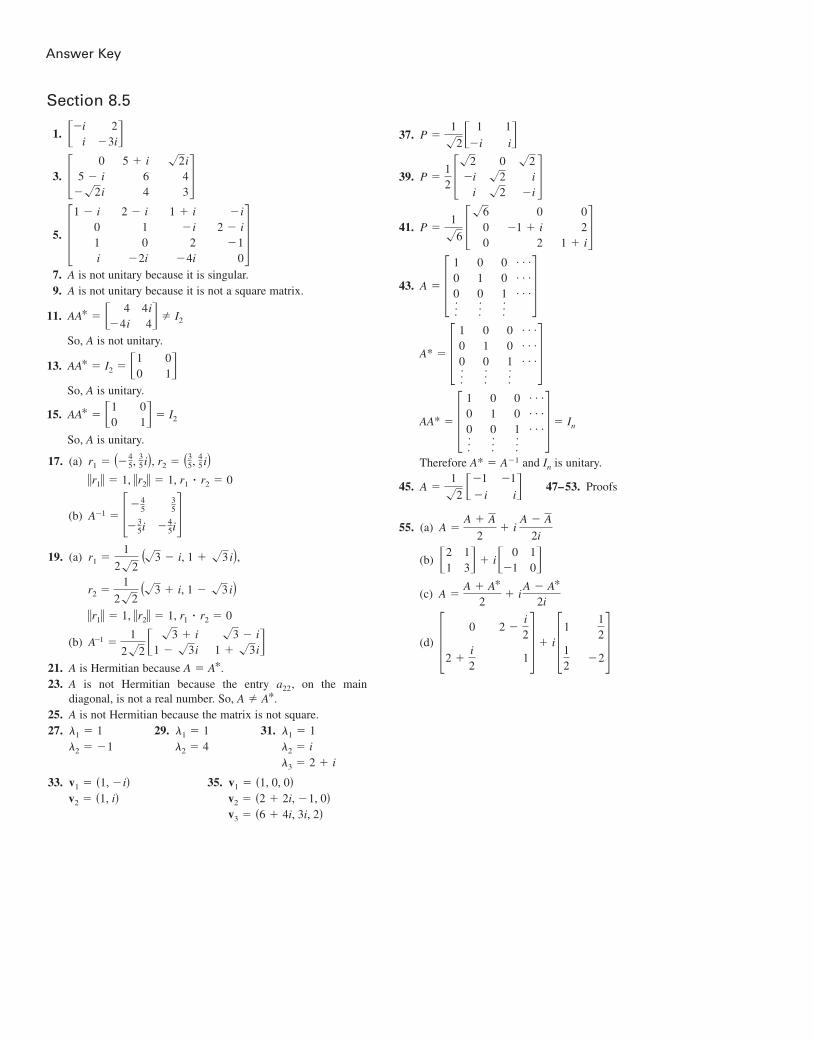
Answer Key
17. (a)
(b)
19. (a)
(b)
21. is Hermitian because 23. is not Hermitian because the entry on the main
diagonal, is not a real number. So,25. is not Hermitian because the matrix is not square.27. 29. 31.
33. 35.
37.
39.
41.
43.
Therefore and is unitary.
45. 47–53. Proofs
55. (a)
(b)
(c)
(d) � i �1
12
12
�2�� 0
2 �i2
2 �i2
1�A �
A � A*
2� i
A � A*
2i
�21
13� � i� 0
�110�
A �A � A
2� i
A � A
2i
A �1�2 ��1
�i
�1
i�InA* � A�1
AA* � �100...
010...
001...
. . .. . .. . .� � In
A* � �100...
010...
001...
. . .. . .. . .�
A � �100...
010...
001...
. . .. . .. . .�
P �1�6 �
�600
0�1 � i
2
02
1 � i�
P �12 �
�2�i
i
0�2�2
�2i
�i�
P �1�2�
1
�i
1
i�
v3 � �6 � 4i, 3i, 2�v2 � �2 � 2i, �1, 0�v2 � �1, i�v1 � �1, 0, 0�v1 � �1, �i�
3 � 2 � i2 � i2 � 42 � �11 � 11 � 11 � 1
AA � A*.
a22,AA � A*.A
A�1 �1
2�2 ��3 � i
1 � �3i�3 � i
1 � �3i��r1� � 1, �r2� � 1, r1 � r2 � 0
r2 �1
2�2��3 � i, 1 � �3 i�
r1 �1
2�2��3 � i, 1 � �3 i�,
A�1 � ��45
�35i
35
�45i�
�r1� � 1, �r2� � 1, r1 � r2 � 0
r1 � ��45, 35i�, r2 � �3
5, 45i�
9781133110873_08_ANS.qxd 3/10/12 6:58 AM Page A6
Section 8.5
1.
3.
5.
7. is not unitary because it is singular.9. is not unitary because it is not a square matrix.
11.
So, A is not unitary.
13.
So, A is unitary.
15.
So, A is unitary.
AA* � �10
01� � I2
AA* � I2 � �10
01�
AA* � � 4�4i
4i4� � I2
AA
�1 � i
01i
2 � i10
�2i
1 � i�i
2�4i
�i2 � i
�10�
�0
5 � i��2i
5 � i64
�2i43�
��ii
2�3i�

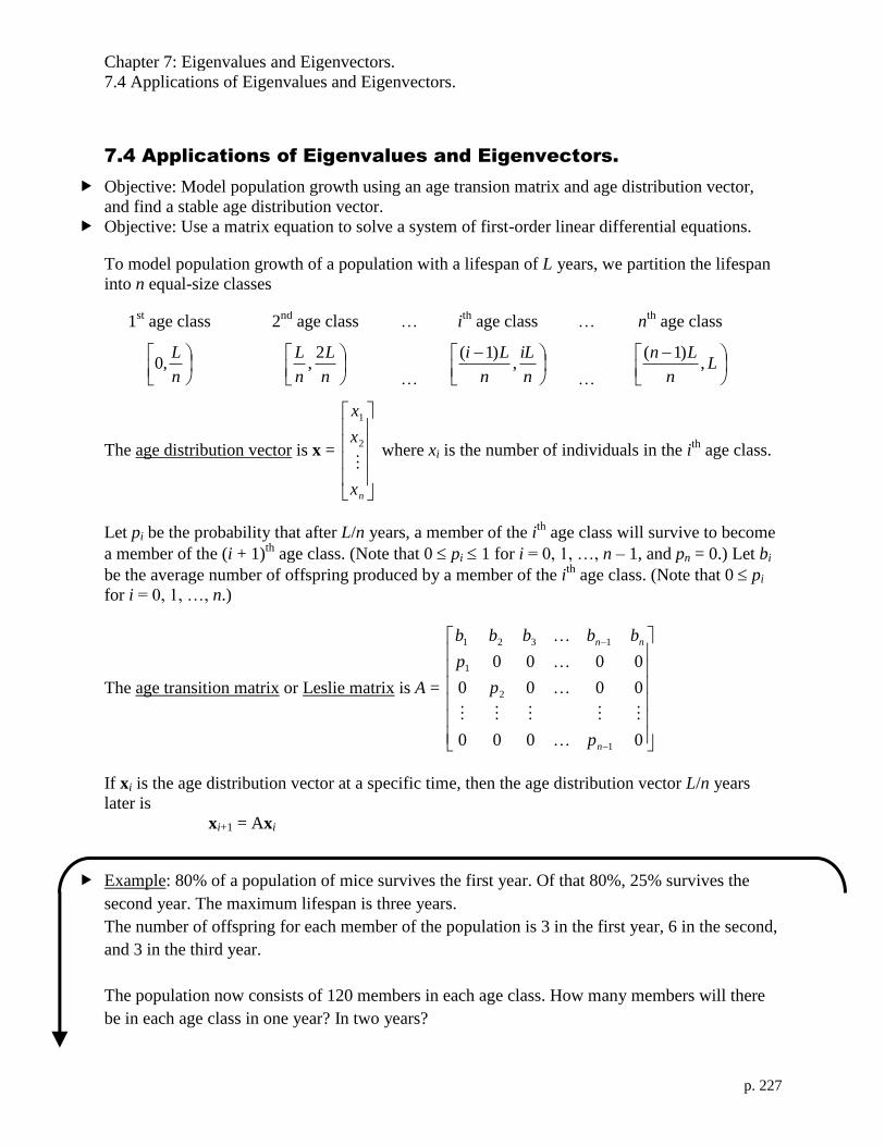
Chapter 7: Eigenvalues and Eigenvectors.
7.4 Applications of Eigenvalues and Eigenvectors.
p. 227
7.4 Applications of Eigenvalues and Eigenvectors.
Objective: Model population growth using an age transion matrix and age distribution vector,
and find a stable age distribution vector.
Objective: Use a matrix equation to solve a system of first-order linear differential equations.
To model population growth of a population with a lifespan of L years, we partition the lifespan
into n equal-size classes
1st age class 2
nd age class … i
th age class … n
th age class
n
L,0
n
L
n
L 2,
…
n
iL
n
Li,
)1(
…
L
n
Ln,
)1(
The age distribution vector is x =
nx
x
x
2
1
where xi is the number of individuals in the ith
age class.
Let pi be the probability that after L/n years, a member of the ith
age class will survive to become
a member of the (i + 1)th
age class. (Note that 0 pi 1 for i = 0, 1, …, n – 1, and pn = 0.) Let bi
be the average number of offspring produced by a member of the ith
age class. (Note that 0 pi
for i = 0, 1, …, n.)
The age transition matrix or Leslie matrix is A =
0000
0000
0000
1
2
1
1321
n
nn
p
p
p
bbbbb
If xi is the age distribution vector at a specific time, then the age distribution vector L/n years
later is
xi+1 = Axi
Example: 80% of a population of mice survives the first year. Of that 80%, 25% survives the
second year. The maximum lifespan is three years.
The number of offspring for each member of the population is 3 in the first year, 6 in the second,
and 3 in the third year.
The population now consists of 120 members in each age class. How many members will there
be in each age class in one year? In two years?
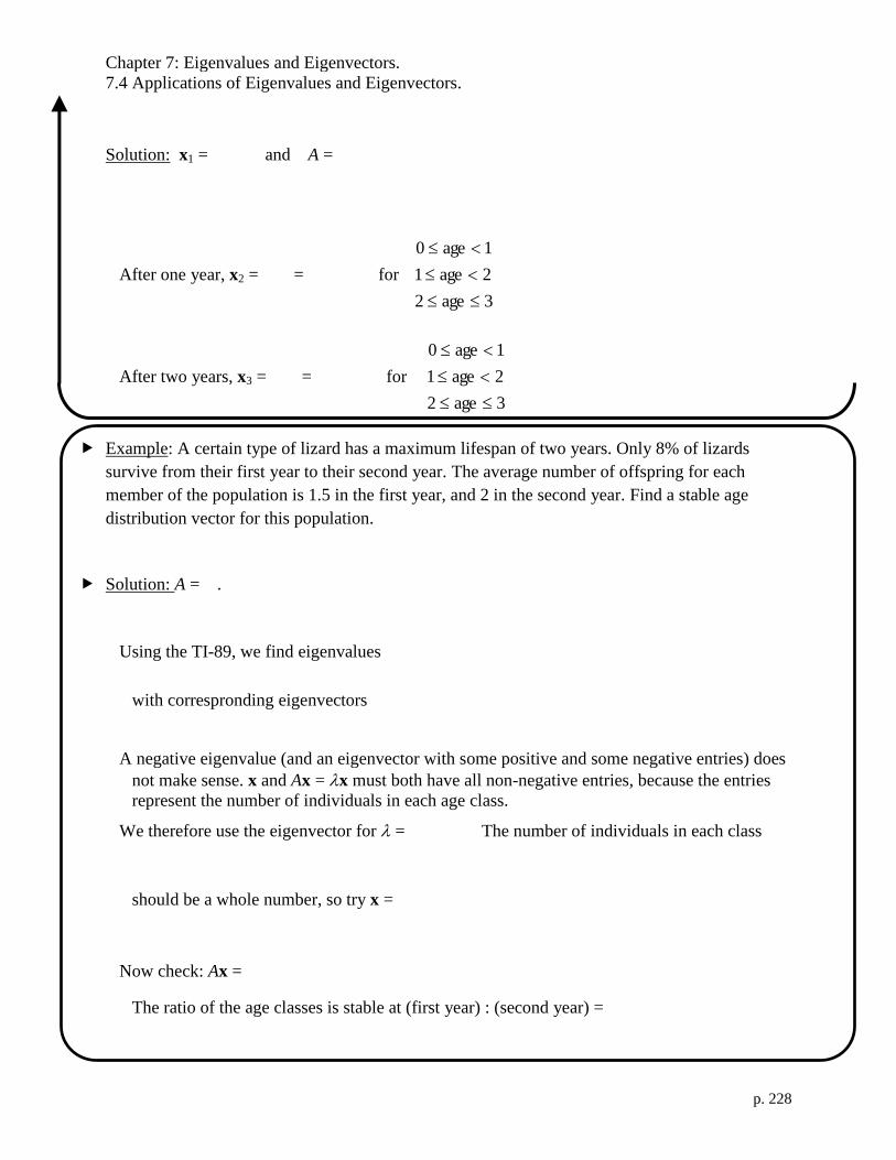
Chapter 7: Eigenvalues and Eigenvectors.
7.4 Applications of Eigenvalues and Eigenvectors.
p. 228
Solution: x1 = and A =
After one year, x2 = = for
3age2
2age1
1age0
After two years, x3 = = for
3age2
2age1
1age0
Example: A certain type of lizard has a maximum lifespan of two years. Only 8% of lizards
survive from their first year to their second year. The average number of offspring for each
member of the population is 1.5 in the first year, and 2 in the second year. Find a stable age
distribution vector for this population.
Solution: A = .
Using the TI-89, we find eigenvalues
with correspronding eigenvectors
A negative eigenvalue (and an eigenvector with some positive and some negative entries) does
not make sense. x and Ax = x must both have all non-negative entries, because the entries
represent the number of individuals in each age class.
We therefore use the eigenvector for = The number of individuals in each class
should be a whole number, so try x =
Now check: Ax =
The ratio of the age classes is stable at (first year) : (second year) =

Chapter 7: Eigenvalues and Eigenvectors.
7.4 Applications of Eigenvalues and Eigenvectors.
p. 229
A system of first-order linear differential equations has the form
nnnnnn
nn
nn
yayayay
yayayay
yayayay
2211
22221212
12121111
with initial conditions
nn Cy
Cy
Cy
)0(
)0(
)0(
22
11
Where each iy is a function of t and dt
dyy i
i .
This is a linear system because the y′ =
ny
y
y
2
1
is a linear transformation of y =
ny
y
y
2
1
.
y′(t) = Ay(t), where A is a matrix of constants.
These are first-order differential equations because they contain first (and not higher)
derivatives.
Example: Solve the system
33213
32212
32111
00
00
00
yyyy
yyyy
yyyy
with initial conditions
33
22
11
)0(
)0(
)0(
Cy
Cy
Cy
Solution:
From calculus, we know that the general solution to y′(t) = ky(t) is y(t) = Cekt.
So the solution to the system (with a diagonal matrix) is t
eCty 1
11 )(
t
eCty 2
22 )(
t
eCty 3
33 )(
Example: Solve the system
313
212
3211 2
yyy
yyy
yyyy
with initial conditions
2)0(
1)0(
4)0(
3
2
1
y
y
y

Chapter 7: Eigenvalues and Eigenvectors.
7.4 Applications of Eigenvalues and Eigenvectors.
p. 230
Solution:
y′(t) = Ay(t), where A =
101
011
112
and y(0) =
2
1
4
Try a substitution y(t) = Pw(t), where P is some invertible constant matrix.
Then y′(t) = Pw′(t) and P–1
y′(t) = w′(t) so
y′(t) = A y(t)
P–1
y′(t) = P–1
A y(t)
w′(t) = P–1
A(Pw(t))
w′(t) = (P–1
AP)w(t)
If is P–1
AP diagonal, i.e. P–1
AP = D =
3
2
1
00
00
00
, then w(t) =
t
t
t
eB
eB
eB
3
2
1
3
2
1
for unknown
constants B1, B2, B3.
Using the TI-89 to find the eigenvalues and eigenvectors of A, we find
P =
707107.057735.0408248.0
707107.057735.0408248.0
057735.0816497.0
and D =
100
000
003
So w(t) =
t
t
eB
B
eB
3
2
3
1
, y(t) = Pw(t) = P
t
t
eB
B
eB
3
2
3
1
, and
y(0) =
2
1
4
= P
3
2
1
B
B
B
, so
3
2
1
B
B
B
= P–1
2
1
4
=
0.707107
0.57735
4.49073
Then y(t) = Pw(t) = P
t
t
e.
.
e.
7071070
577350
490734
=
t
t
t
e
e
e
3
3
3
833.15.03333.0
833.15.03333.0
667.33333.0
=
t
t
t
e
e
e
3
611
21
31
3
611
21
31
3
311
31
Other software may yield other P and D matrices, but w(t) will always be the same.
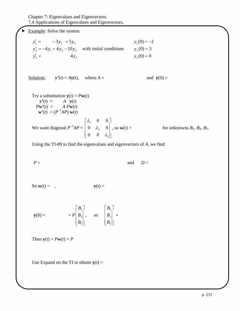
Chapter 7: Eigenvalues and Eigenvectors.
7.4 Applications of Eigenvalues and Eigenvectors.
p. 231
Example: Solve the system
33
3212
321
4
1044
53
yy
yyyy
yyy
with initial conditions
0)0(
3)0(
2)0(
3
2
1
y
y
y
Solution: y′(t) = Ay(t), where A = and y(0) =
Try a substitution y(t) = Pw(t)
y′(t) = A y(t)
Pw′(t) = A Pw(t)
w′(t) = (P–1
AP) w(t)
We want diagonal P–1
AP =
3
2
1
00
00
00
, so w(t) = for unknowns B1, B2, B3.
Using the TI-89 to find the eigenvalues and eigenvectors of A, we find
P = and D =
So w(t) = , y(t) =
y(0) = = P
3
2
1
B
B
B
, so
3
2
1
B
B
B
=
Then y(t) = Pw(t) = P
Use Expand on the TI to obtain y(t) =

Chapter 7: Eigenvalues and Eigenvectors.
7.4 Applications of Eigenvalues and Eigenvectors.
p. 232
An example from continuum mechanics of a
symmetric matrix is the stress tensor
T =
333231
232221
131211
.
The figure uses the notation that T: R3 R3
is the linear transformation iTi eTe
)(
ij is the force per unit area on the plan
perpendicular to ei, in the ej direction.
ii is is a pressure or normal stress. ij is a
shearing stress for i j. T is symmetric
because of conservation of angular
momentum.
Example: Let T =
103
014
341
.
Use the TI-89 to diagonalize T: P =
8042426404242640
6056568505656850
070710707071070
.. .
...
..
=
54
25
3
25
3
53
25
4
25
4
25
5
25
5 0
and D =
100
060
0011
The mutually orthogonal vectors p1 =
4242640
5656850
7071070
.
.
.
, p1 =
4242640
5656850
7071070
.
.
.
, and p3 =
80
6.0
0
.
are called the principal directions, where the stress vector )( ip
T is parallel to pi and where
there are no shear stresses dij for i j. The three stresses 1= 11, 2=6, and 3= 1, are called
principal stresses.

Chapter 7: Eigenvalues and Eigenvectors.
7.4 Applications of Eigenvalues and Eigenvectors.
p. 233
Example (multivariable calculus): The Hessian matrix H of a function of several variables is
symmetric.
If f (x, y): R2 R is a (not necessarily linear) function of two variables, then
H =
2
22
2
2
2
y
f
xy
f
yx
f
x
f
has orthogonal eigenvectors. Near a critical point, the level curves of
f (x, y) = constant are ellipses if the eigenvalues of H have the same sign, a straight lines if
one eigenvalue is zero, or hyperbolas if the eigenvalues have opposite signs. See the text
for more discussion.
f (x, y) = 13x2 –8 xy + 7y
2 – 45
Eigenvalues = 5, 15
Eigenvectors =
1
2,
2
1
f (x, y) = 2𝑥2 + 4𝑥𝑦 + 2𝑦2 + 4√2𝑥 + 4√2𝑦 + 45
Eigenvalues = 0, 4
Eigenvectors =
1
1,
1
1
f (x, y) = 17x2 + 32xy – 7y
2 – 75
Eigenvalues = 25, –15
Eigenvectors =
1
2,
2
1


![[DRAFT] Revised · RE: Revised K-5 Math Curriculum During the 2016-17 and 2017-18 school years, the elementary math committee engaged in a comprehensive review of potential math resources](https://static.fdocuments.net/doc/165x107/5ed71c570066f831634a2dd9/draft-revised-re-revised-k-5-math-curriculum-during-the-2016-17-and-2017-18-school.jpg)


