
HIGH-FIELD EFFECTS IN A METALLIC … EFFECTS IN A METALLIC FERROMAGNET ON ... DOCTOR OF PHILOSOPHY...
248
HIGH-FIELD EFFECTS IN A METALLIC FERROMAGNET ON THE FEMTOSECOND TIMESCALE A DISSERTATION SUBMITTED TO THE DEPARTMENT OF APPLIED PHYSICS AND THE COMMITTEE ON GRADUATE STUDIES OF STANFORD UNIVERSITY IN PARTIAL FULFILLMENT OF THE REQUIREMENTS FOR THE DEGREE OF DOCTOR OF PHILOSOPHY Sara Jean Gamble March 2010
-
Upload
duongkhanh -
Category
Documents
-
view
213 -
download
0
Transcript of HIGH-FIELD EFFECTS IN A METALLIC … EFFECTS IN A METALLIC FERROMAGNET ON ... DOCTOR OF PHILOSOPHY...

HIGH-FIELD EFFECTS IN A METALLIC FERROMAGNET ON
THE FEMTOSECOND TIMESCALE
A DISSERTATION
SUBMITTED TO THE DEPARTMENT OF APPLIED PHYSICS
AND THE COMMITTEE ON GRADUATE STUDIES
OF STANFORD UNIVERSITY
IN PARTIAL FULFILLMENT OF THE REQUIREMENTS
FOR THE DEGREE OF
DOCTOR OF PHILOSOPHY
Sara Jean Gamble
March 2010

iv

Abstract
The dynamics initiated when a magnetic system is excited out of its equilibrium
position are influenced by the strength of the fields driving the excitation and the
timescales over which those fields are applied. This thesis explores dynamics induced
in relatively simple magnetic systems by extremely strong fields applied on ultrafast
timescales. Here, “strong” describes magnetic fields of tens of tesla and electric fields
of gigavolts per meter, and “ultrafast” describes timescales faster than 100 picoseconds
(1 picosecond = 1·10−12 seconds).
Specifically, we look at the process of magnetic switching initiated by strong, true
half-cycle field pulses with temporal durations of either a few picoseconds or a few
hundred femtoseconds (1 femtosecond = 1·10−15 seconds). The experiment utilizes
a single shot technique to initiate the switching which relies on the electromagnetic
fields created by relativistic electron bunches at the SLAC National Accelerator Lab-
oratory. The femtosecond duration pulses have peak magnetic and electric fields of
60T and 20GV/m respectively and coherent frequency spectra which extend into
the terahertz (1 terahertz = 1·1012 Hz). These intense pulses are unique to SLAC
and thus provide us with a novel set of conditions with which to study ultrafast
magnetization dynamics.
While traditional magnetic switching experiments rely on magnetic fields alone to
initiate the switching, the first part of the thesis will discuss a new type of switching
mechanism which utilizes a combination of magnetic and electric fields. We will show
that the 20GV/m electric field of the femtosecond duration electron bunch acts to
create a new, transient magnetic anisotropy axis through a distortion of valence elec-
tron states and that this new anisotropy axis dramatically affects the magnetization
v

switching dynamics induced by the accompanying magnetic field. We will show that
this hybrid switching mechanism triggers a deterministic reversal of the magnetiza-
tion on the timescale of 100’s of femtoseconds, and that the experiment acts as a
proof of principle demonstration for an all electric field induced magnetic switching
technique. While electric fields have been used to manipulate magnetization before,
there has never been a clear demonstration of a technique which would actually use
an electric field to switch. The second part of the thesis will address the rather sur-
prising observation that passage of these ultrafast high-field pulses through our thin
film sample leaves it remarkably damage free, in striking contrast to lower field, longer
pulses which leave signatures of heating. This latter result is particularly encouraging
for potential future applications.
In short, this thesis includes three contributions to the fields of ultrafast magne-
tization dynamics and high-field physics:
1. We observe a new type of transient, all electric field induced magnetic anisotropy
caused by a pure electronic distortion of the valence electron states in a thin film
metallic ferromagnet. This magnetoelectronic anisotropy saturates at a value larger
than any other magnetic anisotropy previously observed in a magnetic metal.
2. We demonstrate the first clear path for an all electric field induced magnetiza-
tion switching technique viable for normal thin film metallic ferromagnets at room
temperature.
3. We show that it is possible to deposit the energy necessary to induce such effects
in a thin film and dissipate it before it can cause appreciable heating of the sample.
We propose coherent transition radiation as the possible dissipation channel.
vi

Acknowledgements
When I consider the people most important to me as family, friends, mentors, or some
combination thereof, there are very few of them whom did not either influence the
path that lead to me attending graduate school or contribute to the (in retrospect
somewhat unbelievable) time I have had completing it. With this in mind, it is
impossible to condense all of the acknowledgements I would like to compose down to
a few paragraphs. Thus, before I say anything specific, I want to say thank you to my
family who always encouraged me to do anything I wanted, my friends who told me
I owned one too many pieces of science fiction paraphernalia to do anything except
physics, and the teachers who showed me how to go about doing it to good end. It
was a delicate balance between all of these that lead to the completion of this thesis
and in that sense I really am a bit indebted to everyone.
I want to first give a joint thank you to my advisor Joachim Stohr and my unofficial
co-advisor Hans Christoph Siegmann. When I arrived at Stanford I was far from set on
studying one particular area of physics and was definitely shopping for a thesis field. It
was with this impressionable mind-set that I started attending the weekly Stohr group
meetings. While I can now say without shame that I had absolutely no idea what was
going on during those first months, two things were obvious. First, it was clear that Jo
and Hans were more excited to spend hours discussing everything from fundamental
physics to the next great idea than any other people I had ever encountered. Second,
it was apparent that either by deliberate or self selection (I’m still not sure) the group
filled with people carrying the same genuine outward enthusiasm for physics. In that
type of situation it is inevitable that the science become appealing. So my first thank
you is to Jo and Hans for assembling the environment that convinced me there is
vii

nothing more exciting to study than magnetism.
My second thank you is to Jo is for the years of not just specific advice but also
general guidance on how to select and approach the right problems. I truly believe
that this thesis is an ideal combination of big picture physics and painstaking detail
and in retrospect both of those have been essential to my education. I also want to
thank Jo for the countless small things he has done over the years to make graduate
school’s rougher points a bit easier. Whether it was bringing Mark and me that space
heater for those long nights in the meat-locker of the FFTB control room, or writing
me e-mails in ludicrously large fonts when I had that bout of iritis, all of those little
things are remembered and appreciated.
I honestly do not know how to begin properly acknowledging Hans. At a basic
level he provided the idea and drive behind this project and was always happy and
enthusiastic to begin a day of work. He taught me how to carefully walk through
a physics problem, he taught me when it was ok to get frustrated (often with the
appropriate German swear words), and, in retrospect most importantly, he taught
me how to have confidence in my work and results. I imagine he would also be upset
if I did not include in this list that he taught me under very certain (and very stacked)
circumstances Swiss truffles can beat Belgian pralines in a coffee time taste test. He
also always provided perspective. Sometimes it was perspective on how to handle
the ten sides of a project in the air at once, sometimes it was perspective on how to
compose a well rounded life, and sometimes it was perspective on how to do both
of these previous things simultaneously. He could always distill any problem down
to basic physics and often astounded me by reducing several of my most difficult
questions down to concepts covered in his freshman physics lectures. This is a skill
I am still working on and know I will continue to apply long after graduate school.
I had the privilege of working with Hans everyday, and he truly made every day a
joy. Every time I walk into building 137 I still find that my head instinctively turns
to the left to look down the hallway to his office to see if his door is open. I wish he
could have seen me finish my graduate work, but I can say (with confidence!) that
he would have been happy with the way things worked out.
I also want to thank our wonderful collaborators on this project as without them
viii

this thesis would not have been possible. Alexander Kashuba was invaluable in both
the interpretation and modeling of the data. It is in large part due to his ideas and
help that this thesis exists. Rolf Allenspach spent countless hours imaging our samples
and discussing the results. He has always been unbelievably patient and meticulous
in both answering all of my questions and reviewing drafts of papers and chapters
of this thesis. Like all experiments, this one would not have been possible without
samples, and for that I thank Stuart Parkin for making our beautiful single crystalline
films. I also want to thank Mark Burkhardt for being there with me during those cold
nights in the FFTB and for being a wonderful help during the early stages of the data
interpretation. I also want to thank Ioan Tudosa for passing on the graduate student
role in this project, Gerry Collet for help building our sample chamber, and Clive
Field and Rick Iverson for help focusing and measuring the profile of the electron
beam.
I am unbelievably indebted to everyone in Stohr group. Current and former
members in a mix of chronological and alphabetical order with whom I have been
lucky enough to work with are: Scott Andrews, Ioan Tudosa, John Paul Strachan, Bill
Schlotter, Venkatesh Chembrolu, Xiaowei Yu, Mark Burkhardt, Ramon Rick, David
Bernstein, Diling Zhu, Benny Wu, Cat Graves, Roopali Kukreja, Tianhan Wang,
Yves Acremann, Bjorn Brauer, Hermann Durr, Suman Hossain, Hendrik Ohldag,
Shampa Sarkar, Andreas Scherz, and Ashwin Tulapurkar. They have all taught me
that science is (at least relatively) easy when you are surrounded by the right people. I
also need to thank all of them for putting up with my paper party hats for every group
birthday, listening to countless stories about munchkins and bunnies, and always
being wonderful lunch and coffee time companions.
Without an amazing administrative staff my hybrid Stanford/SLAC existence
would not have been possible. For that I am grateful to Paula Perron, Claire Nicholas,
Michelle Montalvo, Jennifer Prindiville, Irene Hu, and Amita Gupta. I have also
spent more than my fair share of time talking with all of them in their offices and
have enjoyed every minute of it.
I also want to thank Malcolm Beasley and Philip Bucksbaum for reading this
thesis and always being excited about the project and results.
ix

I have also been lucky to meet several truly wonderful friends during my time at
Stanford. Whether we were partying into the late evening hours or doing problem
sets until the early morning ones, we were always having fun. I specifically want to
thank Guillaume Chabot-Couture, Ann Erickson, Chad Giacomozzi, Ginel Hill, Praj
Kulkarni, Stephanie Majewski, Jamie Mak, Mike Minar, Eugene Motoyama, Matthew
Wheeler, and Tommer Wizansky for a great first six years of friendship. I can assure
you, and everyone else that I don’t have space to name, that you are not getting rid
of me after graduation. I also want to thank Reba Abraham, Shanna Crankshaw,
Steve Harsany, and Stacey Yoder for always being there through good times and bad,
and often through several time zones.
Finally, and most importantly I want to thank my family. Mommy and Daddy,
I am so lucky to have had you as parents. You taught me how to work right and
how to love right and you would not believe how important both of those have been
in getting through graduate school. So much of this is owed to you. Julie, you have
been a wonderful sister and wonderful friend. Even though I know the only reason
you ever walked through the UF physics building was because it was a shortcut with
air conditioning, I hope you still enjoy flipping through this thesis (there’s lots of pink
in it)! E-Ma, thank you for always being so proud of me, and always asking when
I’m coming home. Geert, you know I love you more than anything and I hope you
know how much you have helped me get to this point. I cannot count the things I am
grateful to you for, but they span the gamut from being my best friend to somehow
always knowing how to do the integral I’ve come home with a headache over. I also
want to thank you for sharing your wonderful family with me, and thank the Vrijsens
for being just as excited about my graduation as I am. And, finally, to Bessie, Bub-
bles, Nacho Supreme, and Con Queso, thank you for being my favorite four legged
friends and always bringing a smile to my face with your ceaseless nose wiggles and
binkies.
Sara Jean Gamble
March 10, 2010
x

Contents
Abstract v
Acknowledgements vii
1 Motivation and Introduction 1
2 Introduction to Magnetic Switching Dynamics 5
2.1 Principles of Magnetic Switching . . . . . . . . . . . . . . . . . . . . 5
2.2 Precessional Magnetic Switching . . . . . . . . . . . . . . . . . . . . . 8
2.3 The Landau-Lifshitz-Gilbert Equation . . . . . . . . . . . . . . . . . 9
2.4 Magnetic Anisotropies . . . . . . . . . . . . . . . . . . . . . . . . . . 14
2.5 The Three-Step Model . . . . . . . . . . . . . . . . . . . . . . . . . . 17
2.6 Switching with Electron Pulses . . . . . . . . . . . . . . . . . . . . . 25
3 Previous Work and Simple Calculations 33
3.1 Previous Picosecond Pulse Work . . . . . . . . . . . . . . . . . . . . . 33
3.2 First Models for Switching Behavior . . . . . . . . . . . . . . . . . . . 37
3.2.1 Simple Hand Calculations . . . . . . . . . . . . . . . . . . . . 37
3.2.2 Breakdown of the Simple Model - Damping . . . . . . . . . . 39
3.3 Spin Wave Instability Modeling . . . . . . . . . . . . . . . . . . . . . 42
3.3.1 General Modeling . . . . . . . . . . . . . . . . . . . . . . . . . 42
3.3.2 Spin Wave Instability Modeling and the Present Experiment . 43
3.4 Precession During the Excitation Pulse . . . . . . . . . . . . . . . . . 44
xi

4 Experimental Set-up 47
4.1 The Stanford Linear Accelerator . . . . . . . . . . . . . . . . . . . . . 47
4.2 Experimental Set-up . . . . . . . . . . . . . . . . . . . . . . . . . . . 52
4.3 Electromagnetic Field of an Electron Bunch . . . . . . . . . . . . . . 59
4.4 Relativistic Electromagnetic Field Contraction . . . . . . . . . . . . . 63
5 Experimental Results 69
5.1 Sample Characterization . . . . . . . . . . . . . . . . . . . . . . . . . 69
5.2 Spin-Polarized Scanning Electron Microscopy . . . . . . . . . . . . . 70
5.3 Experimental Data . . . . . . . . . . . . . . . . . . . . . . . . . . . . 77
6 Electric Field Induced Magnetoelectronic Anisotropy 85
6.1 Manipulating Magnetic Anisotropy . . . . . . . . . . . . . . . . . . . 86
6.2 Qualitative Data Analysis . . . . . . . . . . . . . . . . . . . . . . . . 89
6.3 Symmetry Considerations and Simple Modeling . . . . . . . . . . . . 97
6.4 Quantitative Data Analysis . . . . . . . . . . . . . . . . . . . . . . . 100
6.5 Quantitative Analysis - Estimation Method . . . . . . . . . . . . . . . 106
6.6 On All Electric Field Induced Magnetic Switching . . . . . . . . . . . 111
7 Single Electron Energy Loss Mechanisms 115
7.0.1 Motivation for Consideration of the Heating Problem . . . . . 115
7.0.2 Framing of the Energy Loss Problem . . . . . . . . . . . . . . 116
7.1 Introduction to Energy Loss Concepts . . . . . . . . . . . . . . . . . 117
7.2 Collision and Radiative Stopping Powers . . . . . . . . . . . . . . . . 120
7.3 Monte Carlo Methods . . . . . . . . . . . . . . . . . . . . . . . . . . 124
7.4 EGS5 Simulation Procedure . . . . . . . . . . . . . . . . . . . . . . . 126
7.5 Restricted Stopping Powers . . . . . . . . . . . . . . . . . . . . . . . 134
7.6 EGS5 Simulation Results . . . . . . . . . . . . . . . . . . . . . . . . . 135
7.7 General Discussion of Simulation Results . . . . . . . . . . . . . . . . 138
7.8 Time Dependence and EGS Simulations . . . . . . . . . . . . . . . . 140
xii

8 Coherent Effects: Excitations & Radiations 141
8.1 The Method of Virtual Photons . . . . . . . . . . . . . . . . . . . . . 142
8.2 Incoherent Virtual Photon Spectrum . . . . . . . . . . . . . . . . . . 145
8.2.1 Incoherent Spectrum Calculation . . . . . . . . . . . . . . . . 145
8.2.2 Incoherent Spectrum Discussion . . . . . . . . . . . . . . . . . 151
8.3 Coherent Virtual Photon Spectrum . . . . . . . . . . . . . . . . . . . 155
8.3.1 Coherent Spectrum Calculation . . . . . . . . . . . . . . . . . 155
8.3.2 Coherent Spectrum Discussion . . . . . . . . . . . . . . . . . . 158
8.4 Total Virtual Photon Spectrum . . . . . . . . . . . . . . . . . . . . . 161
8.5 Terahertz Science - A Brief Introduction . . . . . . . . . . . . . . . . 165
8.6 Traditional THz Sources vs. the SLAC Beam . . . . . . . . . . . . . 171
8.7 Possible Resolution of the Heating Dilemma . . . . . . . . . . . . . . 174
8.7.1 High-Field Excitations in a Band Model . . . . . . . . . . . . 177
8.7.2 Coherent THz Transition Radiation . . . . . . . . . . . . . . . 184
8.7.3 Coherent Effects and Heating . . . . . . . . . . . . . . . . . . 203
9 Conclusions 211
A Dielectric Constants & Transition Radiation 215
Bibliography 221
xiii

xiv

List of Tables
3.1 Example Experiment Parameters . . . . . . . . . . . . . . . . . . . . 38
4.1 Characteristics of Non-SLAC Magnetic and Electric Fields . . . . . . 62
7.1 NIST Stopping Powers for Co70Fe30 . . . . . . . . . . . . . . . . . . . 122
7.2 EGS Energy Deposition Results for Co70Fe30 On MgO . . . . . . . . 137
7.3 EGS Energy Deposition Results for Free Co70Fe30 Film . . . . . . . . 138
8.1 Times to Cross the Brillouin Zone for Different Electric Fields . . . . 180
8.2 Summary of Energies for Different Coherent Processes . . . . . . . . . 204
A.1 Coherent Transition Radiation Emitted from a Finite ε Radiator . . . 219
xv

xvi

List of Figures
2.1 Modern Hard Drive Image . . . . . . . . . . . . . . . . . . . . . . . . 6
2.2 Schematic of Switching Requirements . . . . . . . . . . . . . . . . . . 7
2.3 Precession of a Magnetic Moment Without Damping . . . . . . . . . 11
2.4 Precession of a Magnetic Moment With Damping . . . . . . . . . . . 13
2.5 Sample Anisotropy Diagram . . . . . . . . . . . . . . . . . . . . . . . 16
2.6 Three-Step Model: First Step . . . . . . . . . . . . . . . . . . . . . . 19
2.7 Three-Step Model: Second Step, No Damping . . . . . . . . . . . . . 20
2.8 Three-Step Model: Second Step, With Damping . . . . . . . . . . . . 22
2.9 Three-Step Model: Third Step . . . . . . . . . . . . . . . . . . . . . . 23
2.10 Three-Step Model: Summary . . . . . . . . . . . . . . . . . . . . . . 24
2.11 Principle of the Experiment . . . . . . . . . . . . . . . . . . . . . . . 26
2.12 In-Plane Electromagnetic Field Components . . . . . . . . . . . . . . 28
2.13 Example In-Plane Uniaxial Switching Pattern . . . . . . . . . . . . . 31
3.1 First In-Plane Data . . . . . . . . . . . . . . . . . . . . . . . . . . . . 35
3.2 Prior Angular Momentum Dissipation Data . . . . . . . . . . . . . . 40
3.3 Energy Dissipation With Precession Angle . . . . . . . . . . . . . . . 41
3.4 Spin Wave Instability Simulation . . . . . . . . . . . . . . . . . . . . 45
4.1 Accelerator Overview . . . . . . . . . . . . . . . . . . . . . . . . . . . 48
4.2 Accelerator Schematic . . . . . . . . . . . . . . . . . . . . . . . . . . 49
4.3 Bunch Compression Process . . . . . . . . . . . . . . . . . . . . . . . 51
4.4 Sample Manipulator and Support . . . . . . . . . . . . . . . . . . . . 53
4.5 Set-up in the FFTB . . . . . . . . . . . . . . . . . . . . . . . . . . . . 54
xvii

4.6 Sample Fork . . . . . . . . . . . . . . . . . . . . . . . . . . . . . . . . 55
4.7 Wire Scanners . . . . . . . . . . . . . . . . . . . . . . . . . . . . . . . 56
4.8 Samples in Experimental Chamber . . . . . . . . . . . . . . . . . . . 57
4.9 E and B Peak Fields for the Short and Long Bunches . . . . . . . . . 61
4.10 Reference Frames for Field Transformations . . . . . . . . . . . . . . 64
4.11 Spatial Contraction of Relativistic Fields . . . . . . . . . . . . . . . . 66
4.12 Set-up Summary . . . . . . . . . . . . . . . . . . . . . . . . . . . . . 67
5.1 SEMPA Microscope . . . . . . . . . . . . . . . . . . . . . . . . . . . . 72
5.2 Mott Technique . . . . . . . . . . . . . . . . . . . . . . . . . . . . . . 75
5.3 Magnetic Contrast Data . . . . . . . . . . . . . . . . . . . . . . . . . 78
5.4 Femtosecond Data Asymmetry . . . . . . . . . . . . . . . . . . . . . . 79
5.5 Topographic Data . . . . . . . . . . . . . . . . . . . . . . . . . . . . . 81
5.6 Zoomed Picosecond Topographic Data . . . . . . . . . . . . . . . . . 82
6.1 Moving Atoms to Manipulate Anisotropy . . . . . . . . . . . . . . . . 87
6.2 Changing Electronic Orbits to Manipulate Anisotropy . . . . . . . . . 88
6.3 Possible Easy Axes Created by the Electric Field . . . . . . . . . . . 92
6.4 Electric Field Induced Effective Magnetic Fields . . . . . . . . . . . . 93
6.5 Motion of M in Electric Field Induced Heff . . . . . . . . . . . . . . 94
6.6 Motion of M Induced by the True B Field . . . . . . . . . . . . . . . 95
6.7 Possible Combined Effects of E and B Fields . . . . . . . . . . . . . . 96
6.8 Symmetries of the B and E Field Torques . . . . . . . . . . . . . . . 98
6.9 Simple Outline of the First Switch . . . . . . . . . . . . . . . . . . . . 99
6.10 Simulated Magnetic Patterns . . . . . . . . . . . . . . . . . . . . . . 102
6.11 Enhanced Damping at Large Angle Precession . . . . . . . . . . . . . 104
6.12 Hand Calculation for Anisotropy Strength, Step 1 . . . . . . . . . . . 107
6.13 Hand Calculation for Anisotropy Strength, Step 2 . . . . . . . . . . . 109
7.1 Co70Fe30 Stopping Power . . . . . . . . . . . . . . . . . . . . . . . . . 121
7.2 Basic EGS Transport Mechanics . . . . . . . . . . . . . . . . . . . . . 129
7.3 Modified Random Hinge Transport Mechanics . . . . . . . . . . . . . 132
xviii

8.1 Concept of Virtual Photons . . . . . . . . . . . . . . . . . . . . . . . 143
8.2 Incoherent and Coherent Fields . . . . . . . . . . . . . . . . . . . . . 147
8.3 Incoherent Virtual Photon Spectrum . . . . . . . . . . . . . . . . . . 152
8.4 Incoherent Virtual Photons vs. Distance . . . . . . . . . . . . . . . . 154
8.5 Coherent Addition of Electron Bunch Fields . . . . . . . . . . . . . . 156
8.6 Coherent Virtual Photon Spectrum . . . . . . . . . . . . . . . . . . . 160
8.7 Coherent Virtual Photons vs. Distance . . . . . . . . . . . . . . . . . 162
8.8 Total Virtual Photon Spectrum . . . . . . . . . . . . . . . . . . . . . 164
8.9 Virtual Photon Spectra for Short and Long Pulses . . . . . . . . . . . 166
8.10 The Electromagnetic Spectrum and its Applications . . . . . . . . . . 167
8.11 Spatial Profile of Coherent THz Virtual Photons . . . . . . . . . . . . 173
8.12 First Brillouin Zone of a 1-d Metal . . . . . . . . . . . . . . . . . . . 177
8.13 Electron Response to a Half-Cycle Pulse . . . . . . . . . . . . . . . . 185
8.14 Schematic for Transition Radiation Production . . . . . . . . . . . . . 186
8.15 Coherent Transition Radiation From a Metal with a Finite Dielectric
Constant . . . . . . . . . . . . . . . . . . . . . . . . . . . . . . . . . . 190
8.16 Form Factor for a Symmetric Gaussian Bunch vs. Frequency . . . . . 192
8.17 Qualitative Sample Response to a THz Half-Cycle Pulse . . . . . . . 195
8.18 Correction Factor For a Finite Sized Radiating Disk . . . . . . . . . . 197
8.19 Coherent Transition Radiation for a 1 cm Radiator and τ =70 fs Bunch 198
8.20 Coherent Transition Radiation for a 1 cm Radiator and τ =2.3 ps Bunch200
8.21 Coherent Transition Radiation for a 100 µm Radiator and τ =70 fs Bunch201
8.22 Coherent Transition Radiation for a 100 µm Radiator and τ =2.3 ps
Bunch . . . . . . . . . . . . . . . . . . . . . . . . . . . . . . . . . . . 202
A.1 Real and Imaginary Dielectric Constants for Cobalt in the Infrared . 218
xix

xx

Chapter 1
Motivation and Introduction
The field of magnetization dynamics is one which nearly everyone is familiar with on
some level. On a slow timescale it encompasses everyday activities such as watching
a compass needle move and watching the poles of bar magnets attract or repel each
other. On a faster timescale magnetization dynamics is utilized by anyone clicking
“save” on their computer as their data will be written by appropriately changing the
magnetization of a series of magnetic bits in their hard drive. On an even faster
timescale pulsed magnetic fields provide a mechanism for exploring new regimes of
physics. The timescales of these different processes span some 15 orders of mag-
nitude and this gives the field of magnetization dynamics a plethora of interesting
fundamental phenomena and diversified applications.
This thesis explores magnetization dynamics in the regime of ultrastrong fields on
ultrafast timescales. Specifically, we consider dynamics induced by magnetic fields in
excess of several tens of tesla applied for either a few picoseconds or a few hundred fem-
toseconds (1 picosecond=1·10−12 seconds and 1 femtosecond=1·10−15 seconds). This
is a largely unexplored realm of magnetization dynamics because common sources of
magnetic fields cannot produce such strong, pulsed fields. Here, we utilize a truly
unique source to conduct our experiment: the Stanford Linear Accelerator. This
three kilometer long electron accelerator gives us access to an unprecedented set of
experimental conditions by accelerating tightly focused bunches of 1010 electrons to
1

2 CHAPTER 1. MOTIVATION AND INTRODUCTION
near the speed of light. These bunches of fast moving charge act as a pulsed cur-
rent source with magnetic fields several times stronger than those of conventional
superconducting magnets and three to four orders of magnitude faster than those of
conventional current carrying wires.
To explore this high-field, ultrafast regime of magnetization dynamics we have
chosen to study how a relatively simple magnetic system “switches” when exposed
to these extreme conditions. To understand the concept of the experiment we thus
need to understand what we mean by “simple” and what we mean by “switches.” We
start with “switches.”
Magnetic switching is like switching for any two-state system. If a system can only
be “off” or “on” or can only be “up” or “down” it is a two-state system and the act
of going from one of these states to the other is a switch. Magnetic switching occurs
when the magnetization rotates by 180 and this can be visualized simply in terms of
bar magnets. If a bar magnet is initially oriented with its north pole pointing to the
left and it is rotated such that its north pole then points to the right, it has switched.
A much more through (and scientific) discussion is contained in chapter two, but this
is the key idea.
Now we can discuss what we mean by “simple.” In this experiment we use a sample
composed of what is essentially an array of bar magnets, each of which is a two-state
system. Prior to the experiment we magnetize the sample so all of the magnets point
in the same direction. We then expose the sample to one of the pulses from the linear
accelerator. The pulse excites the magnetization dynamics and, after it has passed,
the magnets will each ultimately settle into one of their two stable states: each will
either be realigned in the original direction or aligned in the direction 180 opposite
to it. Thus, each magnet will have either switched or not switched. One extremely
elegant aspect of this experiment is that we will be able to elucidate the ultrafast
dynamics which occurred during the pulse by only looking at the final, recorded
switching pattern. In this way we can probe dynamics down to the femtosecond
timescale days or even weeks after the dynamics have occurred. How this is done will
be described in detail in the first chapters of the thesis.
When we pass the current pulse through the sample the magnitude and direction

3
of the applied magnetic field will vary depending on each point’s location relative to
the center of the bunch. This means we will actually excite a range of magnetization
dynamics with a single shot and, consequently, that the final switching pattern will
contain a great deal of information. As we will see, each single shot exposure actually
gives us of the order of 105 data points.
While all of our data comes from single shots, we have access to pulses of two dif-
ferent temporal lengths and hence can compare the dynamics induced by two different
excitations. Our “long” pulse has a duration of a few picoseconds and our “short”
pulse has a duration of about 100 femtoseconds. Each of these pulses contains the
same number of electrons but, due to their variable widths, the field strengths are
different. The shorter pulse has the higher peak magnetic field (65T) which, not
surprisingly, induces interesting magnetization dynamics. We will also see that with
the short pulse, but not with the long, the strong electric field inextricably linked
with this magnetic field begins to play a role in the magnetization dynamics. The
electric field of this short pulse reaches 20GV/m and we will see that it induces a
transient, pure electronic structure alteration of the valence electron orbitals of the
sample. This alteration, in turn, produces a novel type of all electric field induced
magnetic anisotropy. This is the first observation of such an anisotropy, it is the
strongest anisotropy of any kind ever observed in a magnetic metal, and its existence
provides us with the first clear path for an all electric field induced magnetic switch-
ing mechanism viable for normal thin film ferromagnetic metals at room temperature.
These results make up the primary contribution of this thesis.
Alongside these magnetic effects we will also show and discuss results pertaining
to the heating and damage of the sample induced by the passage of the pulses. The
passage of the lower field, long pulse leads to some heating and damage of the sample
near the point of bunch impact, while the passage of the higher field, short pulse does
not. We know the sample absorbs energy from short pulse, as its electric field induces
the observed anisotropy, but this energy is somehow dissipated before it can heat the
lattice to produce any observable effects. We will propose and discuss a coherent
radiative effect as a possible explanation for this result.
The thesis is organized a follows: chapters two and three include an introduction

4 CHAPTER 1. MOTIVATION AND INTRODUCTION
to ultrafast magnetic switching and a discussion of previous pertinent experimental
and theoretical work. The details of the experimental set-up at the linear accelera-
tor are discussed in chapter four. Chapter five describes our microscopy technique
and shows our experimental data. At the end of this chapter we outline the two
central questions which arise from the data, and the rest of the thesis is focused on
answering these questions. Chapter six deals with the electric field induced magneto-
electronic anisotropy, and chapters seven and eight deal with the anomalous heating
observations. Chapter nine contains our conclusions.

Chapter 2
Introduction to Magnetic
Switching Dynamics
2.1 Principles of Magnetic Switching
When a ferromagnet switches the orientation of its magnetization reverses by 180.
The process of this reversal not only contains interesting physics, but also holds a great
deal of technological value. Two state systems form the basis of binary information
storage, and in particular modern hard drives use the switching of magnetic states to
retain such information. After the translation of data into its corresponding series of
ones and zeros, the hard drive writes the information in a corresponding series of “up”
and “down” bits. To store any information thus requires the ability to switch bits
from an “up” to a “down” (or “down” to “up”) orientation. A picture of a hard drive
appears in figure 2.1 alongside an example display of adjacent, oppositely magnetized
bits.
The switching process involves the transfer of energy and angular momentum.
Prior to the switch, a ferromagnetic system resides in one stable minimum energy
configuration with some initial value of angular momentum. During the switch, an
external stimulus such as a magnetic field pulse excites the system with enough energy
to overcome the energy barrier separating the initial stable state from the final stable
state (∆ E) and enough angular momentum to rotate the magnetization by 180 (h per
5

6 CHAPTER 2. INTRODUCTION TO MAGNETIC SWITCHING DYNAMICS
Figure 2.1: A Hitachi hard drive is shown on the left of the figure and a depic-tion of adjacent bits’ magnetization is shown on the right. The arm which extendsover the hard drive can switch the direction of the bits by applying a magneticfield. In today’s hard drives, this writing process occurs at ∼1 bit per nanosecond(1 nanosecond =10−9 seconds).
spin). The system then remains in the new stable state in the switched configuration.
Figure 2.2 shows a schematic of the switching process which contains the key ideas of
supplying energy to overcome a potential barrier, and angular momentum to change
the system’s spin.
In practice three primary methods for applying the external stimulus to initiate
switching exist. In the first method an Oersted field supplies the energy and angular
momentum, which makes this method of switching perhaps the most intuitive. It tra-
ditionally involves applying a magnetic field, H, antiparallel to the original direction
of magnetization, M. While a completely antiparallel orientation would not result in
a torque on the magnetization because of the torque’s dependence on the sine of the
angle between M and H, in practice thermal fluctuations tip the magnetization out
of any completely antiparallel configuration and thereby create a finite torque. After
this occurs the magnetization precesses (circles) about the applied and internal fields
and eventually settles parallel to the applied field. The concepts involved in Oersted
switching arise in the specific switching mechanism employed in this thesis, and so
form the bulk of the following discussion.
We do not utilize the remaining two methods, but they are switching by spin
injection and switching by all optical techniques. In spin injection a spin polarized

2.1. PRINCIPLES OF MAGNETIC SWITCHING 7
spin = /2h spin = - /2h
DE
Figure 2.2: For a system to switch it must absorb both energy and angular mo-mentum. Above, the initial configuration of the system is represented by the leftpotential well and the final state by the right. The two wells represent the two stableenergy states and the blue arrows the respective orientation of the spins which differin angular momentum by h.
current passes through the magnetic sample. The relative orientation between the
spin polarization and initial magnetization of the sample can enable the current to
create a torque on the magnetization and transfer the necessary angular momentum
to switch it [1–7]. All optical switching methods are largely still in the theoretical
stages of development. The ideas utilize laser pulses of precisely chosen frequencies,
polarizations, and durations to manipulate the energy and angular momentum of the
magnetic system [8–11]. One experimental realization utilized circularly polarized
light as the angular momentum source but relied on a heating effect, here inextrica-
bly, linked with the laser pulse to switch. Typically circularly polarized laser pulses
cannot carry enough angular momentum to actually switch the magnetization. In this
experiment it is believed that the laser heating brought the system to its Curie point
and the angular momentum supplied by the laser was then enough to tip the system
into the switched configuration as it cooled [12]. While we have not performed any all
optical experiments, the concept of an all electric field induced switching technique is
introduced in chapter six. What we will actually demonstrate with the experiment in

8 CHAPTER 2. INTRODUCTION TO MAGNETIC SWITCHING DYNAMICS
this thesis is a hybrid switching technique which utilizes both magnetic and electric
fields. The effects, however, are separable, demonstrating the feasibility of a pure
electric field induced switching mechanism.
2.2 Precessional Magnetic Switching
To induce the switching in the experiments described in this thesis we use an Oersted
method called precessional switching. There are actually two types of precessional
switching. The first type, which we do not employ, describes a coherent switching
process like that which would occur when a magnetic field is applied antiparallel to
the initial direction of the magnetization. This is the process which was mentioned in
the previous section (for example, see [13]). We use the second type which describes
the switching process when one applies the magnetic field perpendicular to the mag-
netization [14–18]. This is actually the fastest and most efficient way to switch the
direction of the magnetization and we will discuss the process in detail below. During
that discussion and we will see that the method’s effectiveness depends critically on
the duration of the applied field pulse. This means that pulses of the same polarity
and magnitude can potentially result in several switches of the magnetization, de-
pending on their temporal duration. This is in stark contrast to the first technique
in which the switching dynamics cease after the magnetization has rotated into the
direction of the applied field.
To understand how either of these precessional methods work one needs to un-
derstand the basic equation of magnetization dynamics, the Landau-Lifshitz-Gilbert
(LLG) equation so we will introduce it in the next section. In the section following
that, we will describe the sources and characteristics of the magnetic anisotropies
which play a role in how our samples react to an ultrafast field pulse. We will then
describe the switching process by breaking up the dynamics into three steps: dy-
namics during the excitation pulse, dynamics following the pulse, and the eventual
settling of the magnetization into its new stable state. The chapter will conclude
with a section devoted to how this switching process works specifically with ultrafast
magnetic field pulses delivered by the Stanford Linear Accelerator’s electron beam.

2.3. THE LANDAU-LIFSHITZ-GILBERT EQUATION 9
2.3 The Landau-Lifshitz-Gilbert Equation
We need to start the discussion about dynamics by briefly summarizing the units
used in this thesis.
In short, we adopt the units and definitions of the SI system. More specifically,
we measure the magnetic field, H, in [A/m]. We will often convert the units of [A/m]
to Oersteds [Oe] where 1Oersted= 1000 /(4 π) [A/m]=79.59 [A/m]. We measure the
magnetic induction, B, in units of Tesla [T= Vs/m2]. H and B are related in vacuum
by the permeability of free space, µ0 =4π · 10−7 [Vs/Am]. Thus, in vacuum, B=1T
corresponds to H=104 Oe.
The relation between B and H changes as soon as the field permeates a material
and the proportionality constant µ0 alone no longer suffices. To adequately describe
the fields in matter, we need a third field vector, the magnetization M. The units of
M, unfortunately, are not consistently defined between different major texts, despite
the consistent use of SI units. Here, we will strictly use the relation where M has
the same units as B: [T]. Equation 2.1 gives the full relation of the field vectors in
matter:
B = µ0H + M (2.1)
We also need to define the magnetic moment, m. We use it as representing the
magnetization M multiplied by the volume of the sample. Equation 2.2 shows this,
and gives us the units of m as [Vsm].
m = MV (2.2)
In our convention m and the Bohr magneton, µB, have the same units. Specifically,
µB =eµ0h / 2me =1.17 · 10−29 [Vms], which means 1Vms =0.855 · 1029 µB.
The above units and relations combined with the use of energy densities with
units [J/m3] make up the bulk of what we will need to discuss everything contained
in this thesis. We will describe any other quantities as the need arises.
The discussion of dynamics begins with considering the behavior of a magnetic

10 CHAPTER 2. INTRODUCTION TO MAGNETIC SWITCHING DYNAMICS
dipole moment in a homogeneous magnetic field. With respect to forces, the moment
experiences equal but opposite ones on each magnetic pole so no net force acts upon
it. The moment will, however, experience a torque given by equation 2.3:
T = m×H (2.3)
Since torque on a system causes that system’s angular momentum to change, we can
then write this relation as:dL
dt= T = m×H (2.4)
We can also use the empirical relationship of the magnetic moment’s source with a
rotating charge to directly relate the magnetic moment to its angular momentum.
Equation 2.5 gives this relation:
m = γ L (2.5)
Here, γ is known as the gyromagnetic ratio and it has the value of:
γ =qgµ0
2me
(2.6)
where q is the charge of the particle, g the g-factor (which will take values near 2
for all of the samples used here), and me the mass of the electron. We can see from
equation 2.6 that the sign of γ depends on the sign of the charge of the particle. As a
result, for the negative charge of the electron the magnetic moment and the angular
momentum point in opposite directions.
Combining equations 2.4 and 2.5 we arrive at the equation of motion for a magnetic
moment in a magnetic field:dm
dt= γ m × H (2.7)
Equation 2.7 tells us the moment moves around the applied field with a constant
frequency:
ω = γ H (2.8)

2.3. THE LANDAU-LIFSHITZ-GILBERT EQUATION 11
Figure 2.3: Precession of a magnetic moment in a homogeneous magnetic field, H,applied at an initial angle θ. The motion is perpendicular to both M and H andthus sweeps out a cone in time. The radius of the sphere is 1 indicating that themagnitude of the moment is conserved during the precessional motion.
This ω (in [rad/s]) is the Larmor frequency, and this motion is known as Larmor pre-
cession. The Larmor precession frequency plays an important role in magnetization
dynamics as it sets one of the primary timescales of motion. To get an idea of its
magnitude we can use equations 2.6 and 2.8 to find that one spin will precess one full
revolution in a field of 1T in 36 picoseconds (1 ps= 10−12 s). This precessional motion
is shown in figure 2.3.
Equation 2.7 is a general description of the motion of magnetization in an applied
field and it is the first term in the Landau-Lifshitz-Gilbert equation. This equation
cannot form a complete picture of the dynamics of a moment in an applied field,
however, because we know from practical experience that a magnet will eventually
turn into the direction of the applied field. For this to happen there must be an
additional torque perpendicular to both the precessional torque and to m. We call
this the damping torque. For its equation we introduce a phenomenological constant
which we treat like a coefficient of friction in classical physics. Physically, this means
that there is a dissipation mechanism where angular momentum is transferred from

12 CHAPTER 2. INTRODUCTION TO MAGNETIC SWITCHING DYNAMICS
the magnetic system, making the analogy of a magnetic friction quite appropriate.
Equation 2.9 gives the formula for this damping torque with a dissipation constant
C:
Tdamping = C
(m × dm
dt
)(2.9)
The constant C carries dimensions of [Coulomb/(meter·magnetic moment)]. To find
the total torque exerted on a moment, we can add the precessional torque term to
this damping torque term:
Ttotal = (m × H) + C
(m × dm
dt
)(2.10)
Using again the relation of torque to a change in the total angular momentum and the
proportionality of the magnetic moment to an angular momentum we easily arrive
at:
dm
dt= γ (m × H) + C γ
(m × dm
dt
)(2.11)
The second term in equation 2.10 tells us that the influence of the damping torque
is proportional to the the rate of motion of the magnetic moment. The precessional
torque causes this original motion, and this enables us to rewrite equation 2.11 as:
dm
dt= γ (m × H) + C γ2 [m × (m × H)] (2.12)
A simplification of the C γ2 units in front of the second term yields a term we can
write as (new dimensionless constant · γ /m). We call the new dimensionless constant
α. That enables us to rewrite the previous equation as:
dm
dt= γ (m × H) + α
γ
m[m × (m × H)] (2.13)
Now we have a largely complete picture of the dynamics in a constant applied
magnetic field. This means we can describe the precessional motion of the moment
around the field and the damping of that motion into the direction of the field.

2.3. THE LANDAU-LIFSHITZ-GILBERT EQUATION 13
Figure 2.4: The full precession of a magnetic moment in a homogeneous magneticfield with damping is shown. The radius of the sphere is still 1 as in the previousfigure, indicating that the magnitude of the moment is still conserved.
An important caveat of these equations is that they assume the magnitude of the
magnetic moment remains constant. We will discuss a set of conditions that does not
preserve this assumption in the next chapter.
In practice, we often rewrite equation 2.13 with a coefficient of (1 + α2) pre-
ceding the dm/dt term. Typical systems have small damping values which makes
this term negligible. We can nonetheless incorporate it and we finally arrive at the
Landau-Lifshitz-Gilbert (LLG) equation to describe the motion of magnetic moments
in magnetic fields:
dm
dt= γ m × H +
α
m·
[m ×
(m × dm
dt
)](2.14)
For a proof of this final step, see [19]. A plot of the motion determined by equation
2.14 is shown in figure 2.4. From it we can see both the influences of precession and
damping as the moment eventually spirals into the direction of the applied field.

14 CHAPTER 2. INTRODUCTION TO MAGNETIC SWITCHING DYNAMICS
2.4 Magnetic Anisotropies
The H used in equation 2.14 is an “effective field.” Using this term allows us to com-
bine the separate influences of external applied fields and inherent magnetic properties
of the sample into one term, but we have to know how to do this combination. Our
external applied field comes from the linear accelerator through a process covered in
chapter four. This section describes the inherent magnetic properties of our samples
which generate their own fields. The section begins with a discussion of important en-
ergy scales and barriers in the sample and then relates these to the effective magnetic
fields they create.
A combination of influences determine the magnetic properties of a sample. These
include, for example, shape, bonding configuration, mechanical stresses, and strains.
These influences give the magnetization a preferred orientation by making it energet-
ically favorable to lie in a certain plane or along a certain axis. Here, we refer to the
energy difference between this favored (lowest energy) plane or axis and the unfavored
(highest energy) plane or axis as the magnetic anisotropy energy. We call the favored
orientation the easy plane or easy axis, and the unfavored the hard plane or hard axis.
As a result of the easy orientation being a plane or an axis, the energy associated
with the anisotropy must be an even function of the angular difference between the
easy orientation and the magnetization. For instance, if the x axis is the easy axis
then the energy of the magnetic system should be a minimum of the same magnitude
if M is oriented along the +x or −x direction. Correspondingly, the energy should be
at a maximum 90 away from this axis. The same logic is valid for the easy plane. To
satisfy this requirement mathematically we use a series expansion which is an even
function of the angle enclosed by the easy axis (or easy plane) and M. We call this
angle β. We also give each term in the expansion a constant which has dimensions of
[J/m3], making the quantity of interest an energy density. Equation 2.15 shows such
an expansion.
Eani = K1 sin2(β) + K2 sin4(β) + K3 sin6(β)... (2.15)
We use uniaxial thin films here, which means they have one predominant easy axis.

2.4. MAGNETIC ANISOTROPIES 15
In the coordinate system we will use throughout this thesis our easy axis is the x axis,
so our energetically favorable orientations for the magnetization are along the +x and
−x directions. The source of this uniaxial anisotropy is the crystalline structure of
our thin film, so it is a magnetocrystalline anisotropy. Chapter five will contain the
specific strength of the uniaxial anisotropy energy barrier for our sample. Our samples
also have one easy plane. It is the sample plane which, in our coordinate system, is
the x− y plane. The shape of the sample creates this anisotropy so it is simply called
a shape anisotropy. Again, chapter five contains our specific parameters. For now, we
just want to establish the type of anisotropies which play a role in the magnetization
dynamics. Figure 2.5(a) shows a simple picture of the relationship between our sample
plane, easy axis, easy plane, and coordinate system. For additional information about
the sources of magnetic anisotropies see reference [19].
Our ultimate goal is to be able to describe the magnetization dynamics using the
LLG equation, but the LLG equation only allows us to input magnetic fields, not
energies. Thus, to be able to incorporate the effects of magnetic anisotropy energies
in our dynamics equation we need a way of describing these energies in terms of
effective magnetic fields. After doing this, we will be able to use the LLG equation to
describe the dynamics under the influence of both externally applied magnetic fields
and internal anisotropy fields as we will simply be able to add the two together.
To understand the logic behind how to equate these energies to fields we begin with
a situation where the magnetization is in an unstable excited state with respect to the
preferred orientations. This simply means that the magnetization is not lying either
along the easy axis or in the easy plane. Due to the energy minimization principle
these moments will want to relax back to a stable ground state. Relating this energy
minimization problem to one containing a magnetic field is the key to arriving at
an effective magnetic field expression. To describe the relaxation mathematically we
recall that the derivative of an energy with respect to angle gives a torque. Again
using the generic angle β from equation 2.15, and taking terms only up to second
order we have:
∂ Eani
∂ β= 2 K1 sin(β) cos(β) (2.16)

16 CHAPTER 2. INTRODUCTION TO MAGNETIC SWITCHING DYNAMICS
M
Easy Axis AngleEasy Plane Angle
a
b
Uniaxial Magnetocrystalline Anisotropy (x axis)
Shape Anisotropy Easy Plane (x-y plane)
xy
z
xy
z
Figure 2.5: A schematic displaying the two types of anisotropy present in our sampleis shown. Part (a) illustrates that the x axis is the easy axis and the x − y planethe easy plane. The orientations are shown with respect to the sample plane andthe chosen coordinate system. Part (b) shows a possible excited state configurationof the magnetization and the corresponding angles between the magnetization andthe easy plane (pink) and the magnetization and the easy axis (green). These angleswould be used as the respective βs in anisotropy energy density expressions.

2.5. THE THREE-STEP MODEL 17
We can now make a logical connection between this “effective field” torque and
the torque induced by a real field H. Recalling that we can rewrite the cross product
with a sine, we have:
M × H = M H sin(β) (2.17)
where M is the saturation magnetization of the sample. Combining equations 2.16
and 2.17 gives us:
Hani =2 K1
Mcos(β) (2.18)
If the angle between the magnetization and the easy plane and the magnetization
and the easy axis is the same (for example if the magnetization just moved away from
the x axis perfectly into the x − z plane), the angle β is the same for both effective
fields. This gives the K1 term two contributions: the uniaxial anisotropy, Ku, and
the shape anisotropy, Ks. To obtain K1 we simply sum them.
We now have the physical picture necessary to understand the various influences
on the magnetization dynamics and can move on to combining these ideas into a
physical model for the switching process.
2.5 The Three-Step Model
This experiment ultimately switches the magnetization in a process which can be
described in three steps. First, we excite a premagnetized sample with a magnetic
field pulse. Second, we terminate the field pulse and let the magnetization precess
in its excited state. It is in this step that the magnetization can cross the hard axis
barrier (the y axis in our geometry) and thus switch. Third, we let the magnetization
fully relax in the internal anisotropy fields. This section explains each of these steps
in detail by using a “textbook” switching scenario, which is largely identical to the
actual experiment.
We first set up the geometry. As in the previous section, our easy axis is the
x axis and our easy plane the x − y plane. We will also take the sample as pre-
magnetized along the −x direction. The premagnetization is a key step because we

18 CHAPTER 2. INTRODUCTION TO MAGNETIC SWITCHING DYNAMICS
need to know the initial ground state of the system. We apply the exciting mag-
netic field pulse, which we take as square, along the +y axis. We also give the
field pulse a magnitude much greater than the maximum inherent anisotropy fields
of the sample (ie, the anisotropy field values near the hard axis and hard plane
where β ∼ 90). This means none of the inherent anisotropy fields can apprecia-
bly affect the magnetization dynamics while the external field is present. This is
a good assumption as a typical ratio can reach ∼ 30:1, and it allows us to truly
break the dynamics into three distinct steps. We should also note, however, that
while this assumption is a valid one for pulses in the femtosecond range of this thesis
(1 femtosecond=1 ·10−15 seconds), we will also discuss long pulse experiments (where
“long” means picosecond, 1 picosecond=1 ·10−12 seconds) where the assumption is
not valid. This topic is treated in the next chapter.
We also make the assumption that on the femtosecond timescale of the pulsed
excitation we can neglect the damping of the precession. This is also a reasonable
assumption as the magnetization typically will not even precess 1/4 of a full revolution
during the pulse. Correspondingly, the damping during the pulse is quite negligible.
Damping will be accounted for in steps two and three.
With these assumptions in hand we can focus on the dynamics during the field
pulse. We know a magnetic moment will precess in the applied field and by using the
right hand rule we can easily find the direction of this precession. For our configuration
of the moments premagnetized along −x and field applied along +y the torque is in
the −z direction and the motion in the +z direction (because the angular momentum
and magnetic moment point in opposite directions). Thus, the moment will rise out of
the x− y plane and into the positive portion of the x− z plane. In our idealized case,
the moment will precess perfectly without damping until the square pulse terminates.
We call the angle of precession β and we can determine it by using equation 2.8 and
the temporal width of the square pulse, t:
β = ω · t =eµ0
me
Happlied · t (2.19)
Figure 2.6 shows the dynamics through step one.
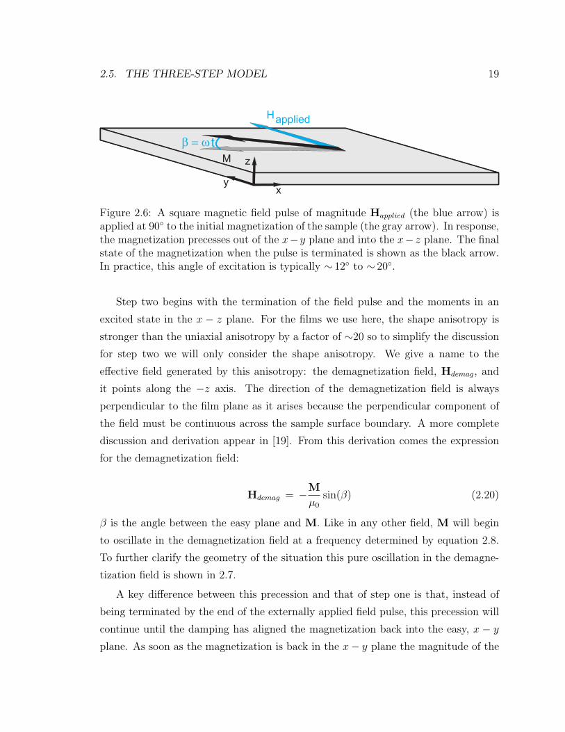
2.5. THE THREE-STEP MODEL 19
M
Happlied
b = w t
xy
z
Figure 2.6: A square magnetic field pulse of magnitude Happlied (the blue arrow) isapplied at 90 to the initial magnetization of the sample (the gray arrow). In response,the magnetization precesses out of the x−y plane and into the x− z plane. The finalstate of the magnetization when the pulse is terminated is shown as the black arrow.In practice, this angle of excitation is typically ∼ 12 to ∼ 20.
Step two begins with the termination of the field pulse and the moments in an
excited state in the x − z plane. For the films we use here, the shape anisotropy is
stronger than the uniaxial anisotropy by a factor of ∼20 so to simplify the discussion
for step two we will only consider the shape anisotropy. We give a name to the
effective field generated by this anisotropy: the demagnetization field, Hdemag, and
it points along the −z axis. The direction of the demagnetization field is always
perpendicular to the film plane as it arises because the perpendicular component of
the field must be continuous across the sample surface boundary. A more complete
discussion and derivation appear in [19]. From this derivation comes the expression
for the demagnetization field:
Hdemag = −M
µ0
sin(β) (2.20)
β is the angle between the easy plane and M. Like in any other field, M will begin
to oscillate in the demagnetization field at a frequency determined by equation 2.8.
To further clarify the geometry of the situation this pure oscillation in the demagne-
tization field is shown in 2.7.
A key difference between this precession and that of step one is that, instead of
being terminated by the end of the externally applied field pulse, this precession will
continue until the damping has aligned the magnetization back into the easy, x − y
plane. As soon as the magnetization is back in the x− y plane the magnitude of the

20 CHAPTER 2. INTRODUCTION TO MAGNETIC SWITCHING DYNAMICS
M
H demag
xy
z
Figure 2.7: If the demagnetization field is the dominant field and the damping isnegligible, the precession of the moments would sweep out a cone like that shownabove.
demagnetization field is zero.
Determining the location in the x− y plane where the magnetization settles given
a certain amount of initial energy involves considering three separate influences: (1)
the strength of the demagnetization field, (2) the strength of the damping, and (3) the
amount of energy a moment must have to cross the hard axis barrier (which we can
think of as extending entirely over the plane x=0). We need to include the influence
of the hard axis barrier as it still takes energy to overcome this energy barrier even
when the moment is out of plane.
We already incorporated the strength of the demagnetization field as it gives us our
precessional frequency. We next add the damping, which ensures the magnetization
will settle back into the x−y plane. The damped motion in the demagnetization field
is shown in figure 2.8. At this point it is useful to recall what we need to know to
determine if the moment switches: the location of this settling relative to the hard, y
axis. Recalling that we premagnetized the film along the −x direction, if the moments
lie on the x > 0 side of the hard axis after step two they switched, and if they lie on

2.5. THE THREE-STEP MODEL 21
the x < 0 side they have effectively not switched.
Thus, we cannot determine the final placement relative to the hard axis by only
including the damping because we need to also account for the energy required in
the magnetic system to overcome the hard axis barrier in each damped precession in
the demagnetization field. Thus, to determine the final placement, we need to know
how much energy we started with. To determine how much energy is deposited in
the magnetic system from the excitation field pulse we can use equation 2.15 along
with the β we obtained from step one. Taking terms to second order, the energy is:
Epulse = (Ku + Ks) sin2(β) (2.21)
To obtain a typical number for our samples, we can take a total anisotropy energy
density of ∼1×10⁶ J/m3 and angle of excitation of ∼12=0.21 rad to get Epulse ≈0.2MJ/m3. For comparison, a typical uniaxial anisotropy energy density for the
samples in this experiment is ∼0.07MJ/m3.
The constraint the energy places on the dynamics is that the moments can only
precess until the damping takes the total energy density to a value below the uniaxial
anisotropy energy density. At that point, there is not enough energy to fully complete
another revolution and the moment will remain on whichever side of the hard axis it
is when this occurs. Notice that figure 2.8 shows the dynamics only up to the point
where the demagnetization field is zero and consequently the energy due to the shape
anisotropy is also zero (because the angle between the magnetization and the easy
plane is zero). This means that the only energy the moment has when it crosses the
easy plane is that of the uniaxial anisotropy, ie Ku times the sine of the angle between
it and the (+ or−)x axis. Since this value will always be smaller than Ku (or equal to
it if this occurs directly along the y axis) the moment will never be able to cross the
hard axis again. At this point the dynamics pertinent to the switching have ceased
and we can commence step three.
Step three commences with the magnetization in the easy plane, but not necessar-
ily along the easy axis. Figure 2.8 shows a possible configuration of the magnetization
when it intercepts the easy plane for the first time. The moment’s exact trajectory

22 CHAPTER 2. INTRODUCTION TO MAGNETIC SWITCHING DYNAMICS
-1 -0.5 0 0.5 1-1
0
1-1
-0.8
-0.6
-0.4
-0.2
0
0.2
0.4
0.6
0.8
1
xy
z
y
a
b
Figure 2.8: The moment precesses in the demagnetization field with an energy muchgreater than it needs to overcome the hard axis created by the uniaxial anisotropy.The motion of step two stops when the moment has reached the easy plane. Part(a) of the figure shows the motion on the sphere of Poincare and part (b) the samemotion with respect to the experiment geometry.

2.5. THE THREE-STEP MODEL 23
-1 -0.5 0 0.5 1
-1
0
1-1
-0.8
-0.6
-0.4
-0.2
0
0.2
0.4
0.6
0.8
1
b
a
xy
zeasy axis
easy axis
Figure 2.9: The moment precesses in the internal anisotropy fields of the sample.The ratio of the major to minor axes of the elliptical trajectory is the same as theratio of the shape and uniaxial anisotropy, here roughly 20:1. Part (a) of the figureagain shows the motion on the sphere of Poincare and part (b) the same motion withrespect to the experiment geometry.

24 CHAPTER 2. INTRODUCTION TO MAGNETIC SWITCHING DYNAMICS
MM
Hanix
y
zM
Happliedb = wt
xy
z
Hdemag
xy
z
1 2 3
Figure 2.10: The figure shows the three distinct steps of the three-step model. Instep one the magnetization is excited by an external field pulse, in step two themagnetization precesses in the demagnetization field and (here) crosses the hard axisbarrier, and in step three the magnetization settles along one orientation of the easy,x axis.
from this point onward depends on the ratio of the shape and uniaxial anisotropy
and on how much energy the moment has when it intercepts the easy plane. Figure
2.9 shows one possible trajectory. We can determine the moment’s initial trajectory
direction immediately after it intercepts the easy plane with the right hand rule. Tak-
ing the magnetization on the positive side of the x axis and the anisotropy field along
the +x axis, we arrive at a torque in the −z direction and thus motion in the +z
direction. The moment will thus move out of the easy plane, as shown in the figure.
As soon as the moment moves out of the easy plane, however, the influence of the
demagnetization field reappears. The result of this interplay is an elliptical trajectory
with the ratio of the major to minor axes being the ratio of the shape to uniaxial
anisotropy, here roughly 20:1. This elliptical motion and its associated damping is
that depicted in figure 2.9. The magnetization ultimately spirals into the easy axis
and at this point all dynamics cease.
For clarity, figure 2.10 depicts the three steps in the switching process side by side.
Here, the magnetization absorbs enough energy to cross the hard axis barrier once
and ultimately settles in the switched configuration.
Now we can understand both why the precessional switching process with the
field applied perpendicular to the original magnetization is the most efficient type of
switching, and why pulses of the same polarity can lead to multiple switches of the
magnetization. The efficiency arises because the torque is at a maximum when m
2.6. SWITCHING WITH ELECTRON PULSES 25
and H are orthogonal to each other. The multiple switches arise because the angle β
by which the moments initially precess out of the x−y plane depends on the duration
of the pulse. Since this determines the amount of energy left in the system, it also
determines how many times the moments will have enough energy to cross the hard-
axis barrier. A slightly longer or shorter pulse can thus make the difference between
an additional switch or the lack thereof.
Here we should note a possible point of confusion with the timescales used in
this thesis. We will refer to “picosecond” (long) and “femtosecond” (short) pulses
and their associated switching patterns. The picosecond or femtosecond timescale,
however, refers ONLY to the duration of the exciting pulse. The actual switching takes
place in step two of this three-step process and it lasts much longer (often far into the
picoseconds) depending on how much energy was deposited and the strength of the
sample’s anisotropy fields. When we refer to our switching process as “ultrafast” we
mean that the amount of time we must apply the external stimulus is ultrafast. This
is also the timescale which is important in technology. For instance, when writing
bits in a hard drive, the write time is the time for which the write head must apply
the magnetic field over the bit. The head can leave this position as soon as the final
orientation of the magnetization is determined. This means the magnetization can
still be precessing when the external field is removed.
2.6 Switching with Electron Pulses
The validity of breaking up the switching dynamics into the three distinct steps
described in the previous section hinges on the external field in step one having a
magnitude strong enough such that it dwarfs internal anisotropy fields. In other
words, the precession time induced by the internal anisotropy fields to make one full
revolution must be substantially longer than that induced by the excitation pulse
for the three-step model to be valid. We can quantify this by finding the precession
frequency in a typical anisotropy field by using equations 2.18 and 2.8. For the
samples considered here, a shape anisotropy energy density of 1.5 MJ/m3 is typical.
This yields a time of 19 ps for one full revolution. Thus, if we have an excitation

26 CHAPTER 2. INTRODUCTION TO MAGNETIC SWITCHING DYNAMICS
~40 mµ
e-beam
28 GeV
140fs - 4.66ps
E
-
BM
Figure 2.11: A bunch of electrons traveling at near the speed of light impacts thesample at normal incidence. The magnetic field excites the moments and the switchingpattern is retained via the principle of magnetic recording.
pulse that causes precession on a comparable picosecond timescale the assumption of
independent pulse driven dynamics in step one would not be a valid one to make. In
this section we will qualitatively and quantitatively discuss the process of switching
with an electron beam. The majority of the work contained in this thesis utilized
electron pulses with durations in the ∼100s of femtoseconds and fields in the 10s of
tesla yielding precession times in the 0.1 - 1 ps range, making the separation of the
three independent steps valid.
Figure 2.11 illustrates the basic principle of the experimental set-up used to switch
a sample with an electron bunch. The techniques for generating the bunches, the
methods we use to characterize them, and the detailed overall set-up are presented
in chapter four. Here, we want to establish the method of excitation in the sample
for which figure 2.11 is sufficient. In the figure an electron bunch moves at near
the speed of light towards the sample. The charged electrons making up this bunch
carry with them both magnetic and electric fields. The directions of these fields are
represented by the red and blue arrows in the figure respectively. Their orientation is
not surprising given that we can think of the bunch as a current pulse traveling down a
normal wire with an Oersted field circling it and an electric field pointing towards the
negative charges. The bunch impacts the premagnetized sample at normal incidence
and thus exposes the moments to the associated fields.

2.6. SWITCHING WITH ELECTRON PULSES 27
The profile of the electromagnetic field of the bunch is “pancake” like, which
means the fields are transverse to the direction of propagation of the bunch. When
the fields reach the sample they consequently lie entirely in the x − y plane of the
film. This feature arises because the bunch is traveling near the speed of light, which
relativistically contracts the profile into the pancake like shape. The equations that
describe this contracted profile are discussed in chapter four. Here we will simply take
the magnetic field as parallel to the surface of the sample at the time of impact and
also assume it penetrates our thin film (for reasons which will also later be discussed).
Elucidating the dynamics which occur while the pulse is inside the sample requires
a combination of the ideas of the previous section and the knowledge of the magnetic
field strength and direction characteristics as a function of the location of the center
of the beam. The full expression for the field generated by the bunch is discussed
in chapter four. Here, however, we can simply leave the field in the generic terms of
Ampere’s law [19]:
H = I
[yr, x
r, 0
]
2π r(2.22)
We can now take the field profile and put it in the context of the experimental
geometry. Figure 2.12 shows the the direction of the fields generated by the beam in
the plane of the sample.
Since we also know we preset the magnetization along the −x direction we can
write the initial magnetization vector as M=[-Ms,0,0]. Here Ms is the saturation
magnetization of the sample, which is the maximum value of magnetization per unit
volume a material can have when all the moments are fully aligned. In our units we
measure this saturation magnetization in tesla, and for our samples it has a value
of 2T. We now take the torque as the cross product of M and H to see that there
is only one component of the torque which emerges to influence the dynamics, that
coming from Hy. Thus,
T = Ms Hy (2.23)
We know Hy because we know the profile of the current creating the magnetic field.

28 CHAPTER 2. INTRODUCTION TO MAGNETIC SWITCHING DYNAMICS
B
EM
a
b
Figure 2.12: The relationship between the sample plane and the magnetic and electricfields generated by the bunch is shown. The fields are in-plane and the directions arefrom the perspective of an observer looking in the direction of bunch propagation. Inour geometry this is into the −z direction. Part (a) of the figure illustrates the fielddirections looking in the −z direction and shows the direction of premagnetizationused in the experiment. Part (b) superimposes the field lines on a 3-d rendering ofour sample geometry to emphasize that the field lines are in truly in-plane.

2.6. SWITCHING WITH ELECTRON PULSES 29
With this we can again use equation 2.8 integrated over time to find the total angle
of precession out of plane of a moment during the field pulse:
β =
∫ ∞
−∞ω dt =
∫ ∞
−∞γ H dt (2.24)
Now we need to substitute the appropriate value of H, which we get from equation
2.22. Taking this along with the knowledge that only the Hy component contributes
to the torque we rewrite equation 2.24 as:
β =
∫ ∞
−∞γ
I(t)
2 π r
x
rdt (2.25)
The integration of this equation is actually much simpler than may be immediately
obvious because the actual task is to integrate the current in the pulse over all time.
This simply yields the total charge in the bunch, or simply the number of electrons
in the bunch, Ne, times the electronic charge. We are then left with:
β = γNe e x
2 π r2(2.26)
or substituting in γ with a g-factor of 2
β =µ0 e2 Ne x
me 2 π r2(2.27)
Keeping in mind that this precession angle β lies entirely in the x − z plane we
can immediately see its relation to the energy absorbed by the sample during the
pulse as E = K1 sin2(β). Thus, equation 2.27 not only describes the location of
moments with a certain out of plane precession angle, but it also describes the lines
of equal energy deposition from the pulse. Since the energy absorbed in step one
of the switching process determines how many revolutions a moment can make in
the demagnetization field in step two, it also determines which side of the hard axis
barrier the moment will lie upon when its energy is below the value needed to cross
the hard axis barrier again. This means that if we plot these lines of equal energy
deposition we will obtain the shape of the regions which ultimately switch. This
process is described in detail in [19].

30 CHAPTER 2. INTRODUCTION TO MAGNETIC SWITCHING DYNAMICS
Before we plot these lines, it is also important to notice that equation 2.27 is
independent of both the shape and temporal duration of the pulse. Both of these
characteristics fall out in the integration over time. According to equation 2.27 the
crucial parameter of the pulse is the number of electrons in it. This becomes critically
important later when we observe striking differences between patterns created with the
same number of electrons but different temporal durations.
We can now take equation 2.27 and look for its solutions when β is constant (ie
the solutions for constant energy deposition). The only variables in the expression
are x and r. This makes the problem equivalent to solving β ∝ x / r2. After some
simple algebra this leaves us with the following expression:
(x − ai
ai
)2
+
(y
ai
)2
= 1 (2.28)
Graphically, the solutions are circles with radii R = ai with centers shifted along
the ± x axis by ai. While the solution set itself is continuous, the pattern we observe
recorded on our thin film will have a more distinct character. Before we show the
solution we can reason that there will be a point on the x axis some distance away
from the center of the beam which will absorb just enough energy from the pulse to
switch once. From equation 2.28 we see that this point is only one on a circular curve
of points which have absorbed the same amount of energy. A point slightly closer to
the beam on the x axis will correspondingly have absorbed slightly more energy and
thus also have enough to switch. As we move closer and closer to the origin, however,
we will reach a point where the moments have absorbed not just enough energy to
switch once, but twice, then three times etc. Each of these points is a member of a
circular curve of solutions. Thus, we can expect a figure-eight type of pattern with
regions of ultimately switched and un-switched points (where the inner un-switched
regions have actually switched two, four, six, etc times leaving them in their original
state).
Figure 2.13 shows what a pattern might look like. The colors here do not represent
a pattern which would be visible to the eye and instead represent a pure magnetic

2.6. SWITCHING WITH ELECTRON PULSES 31
Initial M direction
H
MM
M
H
H
M
H
M
H
H
M
Figure 2.13: A pattern recorded in an in-plane uniaxial thin film might look like theabove. The conditions of the initial magnetization and orientation of the magneticfield are identical to the actual experiment.
contrast. The switched and un-switched circles are shown in pink and white respec-
tively. The imaging technique we use to obtain magnetic contrast images is explained
in chapter five. The conditions shown in the figure are identical to our actual experi-
mental set-up: the magnetization is initially along the −x direction, and the magnetic
field lines circle the origin of our coordinate system in the counter clockwise direction
looking towards the −z axis.
Up to this point we have discussed an ideal switching experiment with minimal
quantitative results. A discussion of how to actually calculate the radii of the circles
is included in the next chapter. Discussions about the influences which cause the

32 CHAPTER 2. INTRODUCTION TO MAGNETIC SWITCHING DYNAMICS
recorded patterns to deviate from this ideal behavior are discussed throughout the
rest of this thesis.

Chapter 3
Previous Work and Simple
Calculations
In the last chapter we described magnetic switching under “textbook” conditions, for
which we had to make some assumptions. We assumed that the switching motion
is deterministic, the damping of precessing moments is constant in time, and the
dynamics after an ultrafast field pulse can be separated into three distinct steps. In
this chapter we are going to discuss deviations from this ideal behavior. We begin by
discussing previous work done to investigate ultrafast switching at the SLAC National
Accelerator Laboratory (SLAC). Considering these results leads us naturally into a
discussion of deviations from the expected behavior. The first two sections deal with
this previous data, and the last three discuss in detail the physical sources of the
deviations. These topics are treated here, as opposed to later in the thesis, because
they are crucial to understanding the shape of the switching patterns, but do not
relate to the specific electric field induced effects which are the new results in this
thesis. We want to discuss these effects now to isolate the new observed effects later.
3.1 Previous Picosecond Pulse Work
Magnetic switching experiments at SLAC have been ongoing since 1995. The earli-
est work utilized 6 ps pulses to generate changes in magnetization in both in-plane
33

34 CHAPTER 3. PREVIOUS WORK AND SIMPLE CALCULATIONS
and perpendicular samples (perpendicular samples have the easy direction of their
magnetization perpendicular to the film plane) [14]. This experiment verified that it
is possible to record magnetic patterns with electron pulses in both types of media,
that the sample suffers some beam damage in the center near the point of impact of
the bunch, and that the perpendicular media can experience a relative spread in the
minimum required switching field of up to thirty percent.
Later work repeated this first experiment on the ps timescale with the perpendic-
ular films and successfully further quantified the early results. This second paper is
reference [20]. The quantification was accomplished by varying both the pulse dura-
tion and internal anisotropy fields of the samples. The authors demonstrated that,
even in films with high exchange coupling, a simple Landau-Lifshitz model which
neglects both the exchange and dipolar coupling can explain the switching behav-
ior. They also found a broadening of the transition region similar to the spread in
switching fields observed in [14]. They conclude the spread is the result of not only
the initial film quality but also inherent physical properties of the system, specifically
phonons.
The work with perpendicular media was continued in [21]. Here, ps pulses were
again used and this time the effect of passing multiple bunches of electrons through the
same location on the films was investigated in detail. A primary result was that the
switching process is not a fully deterministic one, but is actually stochastic. Several
different types of samples were used and all showed the same stochastic switching
behavior. The authors concluded that stochastic switching is a general feature of
ultrafast precessional magnetization switching and that a possible source of the initial
randomness is thermal fluctuation within the magnetic grains of the sample. These
fluctuations include higher order modes where the spins are not parallel to each other.
When the sharp rising edge of the field pulse interacts with the modes, the pre-existing
thermal randomness is amplified and leads to the stochastic behavior.
While the work with perpendicular samples is valuable to the overall understand-
ing of the ultrafast switching process, the work of this thesis utilizes only in-plane
samples so we will now leave the perpendicular media and focus only on in-plane
uniaxial samples.

3.1. PREVIOUS PICOSECOND PULSE WORK 35
Figure 3.1: The figure shows in-plane data from reference [15]. The left side of thefigure shows the experimental magnetic contrast image. The darker regions are theones where the magnetization has switched under the influence of the electron pulse,while the white regions are ones that have not switched from the original directionof premagnetization. The figure-eight pattern is clearly visible as predicted withthe three-step model in chapter two. The right side of the figure shows a patterncalculated with the LLG equation. While the gross features are reproduced, thereare differences which are discussed in detail in reference [15]. The figure is takenfrom [15]. Reprinted with permission from AAAS.
The Science paper in reference [15] treated the behavior of in-plane films in greater
detail than reference [14]. An important difference between these in-plane samples
and the perpendicular ones of the previous papers was that the fields required to
induce a switch were much lower. The perpendicular media required ∼2.5T with a
pulse length of a few picoseconds, while the in-plane media could switch with a field of
only ∼0.25T. This experiment verified that switching is possible in uniaxial thin film
samples with ps pulses. It also introduced the three-step model treated in the previous
chapter. While the expected overall shape of the figure-eight pattern proposed is
observed, it was also found that the inner switches are not well reproduced with a
simple LLG simulation. This is a feature also observed in later experiments, and also
in the new data in this thesis. A set of data from this paper and its corresponding LLG
simulation are shown in figure 3.1. Two main discrepancies are obvious. First, the
calculated pattern shows many more switches towards the center than the recorded
data. Second, the radii of the switched regions are not the same.

36 CHAPTER 3. PREVIOUS WORK AND SIMPLE CALCULATIONS
Reference [15] discusses the discrepancies between the observed data and calcu-
lated pattern at length, so here we only summarize the conclusion: the details of
the inner structure of the patterns cannot be reproduced with a LLG simulation in-
cluding material parameters which do not vary in time. The authors propose a time
dependence of the damping parameter α, and two different mechanisms which would
lead to this dependance are proposed: an excitation of magnons and electron-electron
scattering.
Following the Science paper in 1999, a PRL in 2005 further explored the source of
the unexplained behavior of the switching near the center of the figure-eight pattern in
the high magnetic field regime [22]. The paper deals specifically with the dissipation of
spin angular momentum during the switching process. This dissipation is inherently
linked with α in the LLG equation because the value of α dictates the rate that
angular momentum is transferred from the uniform rotation mode in the spin system.
As mentioned in the paragraph above, usual simulations of magnetization dynamics
utilizing the LLG equation take α as a constant. The value of the constant is usually
taken as that obtained from ferromagnetic resonance (FMR) experiments. FMR often
provides a good value for the damping parameter as it uses small angle excitations
to measure it, and small angle excitations are usually the ones employed in dynamics
studies. Because of the use of the extremely strong field pulses of the SLAC beam,
however, this small angle excitation limitation is far surpassed. Near the edge of
the beam (so near the center of the figure-eight recorded pattern) the magnetization
can be substantially excited out of the easy plane. With the ∼60T fields obtained
with the fs duration pulses the precession angles even approach 90. This opens the
question of whether in this high angle excitation regime an additional pathway for
angular momentum dissipation opens.
The Stamm PRL uses arguments proposed in reference [23] to suggest the in-
creased damping observed in the center of the patterns is caused by the opening of a
dissipation channel from the uniform magnetization precession mode to higher spin
wave (magnon) modes (for an introduction to spin waves see [24]). This channel
is delayed compared to that which transfers angular momentum directly to the lat-
tice, and is thus not observed in experiments which only switch once. In the single

3.2. FIRST MODELS FOR SWITCHING BEHAVIOR 37
switch experiments, there is no time to transfer the momentum into the higher spin
wave modes because the magnetization settles into its easy orientation before the
dissipation can take place.
Before discussing further any results, it is useful to take a moment to go through
a hand calculation which enables us to physically calculate the size of the figure-
eight patterns using only the material parameters of the sample and the number of
electrons in the bunch. After going through this calculation the conclusion reached in
the Stamm PRL regarding increased damping in the high-field regime will logically
follow.
3.2 First Models for Switching Behavior
3.2.1 Simple Hand Calculations
Equation 2.15 from the last chapter gives us the energy deposited in a sample by
an electron beam pulse. In this section we will start from this equation and use the
material parameters of the sample along with the number of electrons in the bunch
to calculate the location of the first switch of an in-plane sample along the x axis.
For the calculation we will take all of the energies as energy densities in [J/m3].
This simplifies obtaining the numbers used in the calculations as all anisotropies are
typically measured as energy densities.
We can take equation 2.15 to second order and arrive at an expression for the
energy density deposited in the sample by the pulse:
Epulse = (Ku + Ks) sin2(β) (3.1)
Using the values from table 3.1 we obtain Epulse = 1.58 sin2(β) MJ/m3.
The energy required to switch once is simply that of the uniaxial anisotropy,
because the hard axis must be crossed once. This is using the assumption of chapter
two that any damping is negligible for the first switch. So, to switch once we can
equate Ku with Epulse:

38 CHAPTER 3. PREVIOUS WORK AND SIMPLE CALCULATIONS
1.6 10·Number of electrons in bunch, N
2g factor (dimensionless)
2 TSaturation Magnetization (Ms)
1.5 MJ/m3Shape Anisotropy (K s)
0.08 MJ/m3Uniaxial Anisotropy (K u)
Number of electrons in bunch, N
2g factor (dimensionless)
2 TSaturation Magnetization (Ms)
1.5 MJ/m3Shape Anisotropy (K s)
0.08 MJ/m3Uniaxial Anisotropy (K u)
e10
Table 3.1: Above are material and beam parameters with values typical for the SLACexperiments with in-plane films. These are the values used in the sample calculationfor the first switch.
Ku = Epulse = 0.08 · 106 = 1.58 · 106 sin2(β) (3.2)
Now we can solve for β. We know for the first switch the angle of elevation is small,
so we will take a small angle approximation. Also, all of these equations have been
derived for angles in radians, so this leaves us with:
β =
√Ku
Epulse
= 0.23 rad (3.3)
This value of β can now be used in equation 2.27:
0.23 =µ0 e2 Ne x
me 2 π r2(3.4)
Since we know the solutions to equation 2.27 are circles shifted along the x axis,
and we are solving for the location of the first switch along the x axis, we can simply
take r as equal to x. This simplifies the above expression to include the term 1/x
instead of x/r2.
0.23 =µ0 e2 Ne
me 2 π x(3.5)
This can simply be solved for x, which is then the diameter of the first switch

3.2. FIRST MODELS FOR SWITCHING BEHAVIOR 39
along the x axis: 367µm. Recalling the overall figure-eight shape of the pattern this
gives a size of ∼740µm along the x axis and ∼370µm along the y axis. This is a very
reasonable size for the in-plane media we use here.
3.2.2 Breakdown of the Simple Model - Damping
While this is a very useful technique for calculating the location of the first switch,
it does not work as well for the inner switches. While the use of the small angle
approximation contributes to the discrepancy, the approach becomes less accurate
primarily because of the neglect of damping. While the moments precess in the
demagnetization field they need energy to not only overcome the hard axis barrier
but also to give up to damping. For the first switch this amount lost to damping is
so small that it can be safely neglected, as we have done above. Repeating the above
calculation for the second switch, however, yields incorrect results showing that the
damping is, by that point, appreciable. Thus, to accurately predict the location of
the higher order switches we need to incorporate the damping. We know this is not a
trivial matter, however, because the experimental data indicates the damping is time
dependent.
It is specifically at this junction that the Stamm PRL begins to address the prob-
lem. The magnetic switching pattern obtained in the experiment is shown in figure
3.2 along with a zoomed image of some of the switching boundaries. Again we see
the overall figure-eight pattern, and again the location of the first switch can be ac-
curately determined with the α from FMR. The approach followed to analyze the
data is the following: Taking data points along the x axis the location of each switch-
ing boundary is determined. The locations were specifically selected using the fitted
circles visible in figure 3.2. We can then take these observed switches along the x
axis and use them in equation 2.27 to solve for the angle necessary to complete each
switch, βi. We can then plot the increase of damping towards the center of the pat-
tern in a meaningful way by saying the energy required for each switch after the first
is the uniaxial anisotropy plus some amount lost to damping, which we will call δ.
We can write the expression as this:

40 CHAPTER 3. PREVIOUS WORK AND SIMPLE CALCULATIONS
(a)
(b)
Figure 3.2: One of the magnetic contrast patterns from reference [22] is shown. Part(a) of the figure shows the entire pattern while part (b) shows a zoomed in view of theboxed portion in (a). The fitted circles shown in white in (b) are used to derive theenergy needed to complete a switch, as discussed in the text. The rather large spotin the center of the pattern with no visible switches is attributed to beam damage,and the left and lower portions of the pattern in part (a) have been disturbed bydomain wall motion after exposure to the beam which results in the black coloring.Reprinted figure with permission from [22]. Copyright 2005 by the American Phys-ical Society. Readers may view, browse, and/or download material for temporarycopying purposes only, provided these uses are for noncommercial personal purposes.Except as provided by law, this material may not be further reproduced, distributed,transmitted, modified, adapted, performed, displayed, published, or sold in whole orpart, without prior written permission from the American Physical Society. Originalmaterial: http://prl.aps.org/abstract/PRL/v94/i19/e197603

3.2. FIRST MODELS FOR SWITCHING BEHAVIOR 41
Figure 3.3: The increase in energy dissipation with time is shown with the uniaxialanisotropy energy density as a scaling factor. This figure comes from reference [22]and the data is shown for the pattern in figure 3.2. This film is 15 monolayers thickand its data points are shown as circles. Additionally shown are data points for a 10monolayer thick film (squares), which is not discussed here. The figure also includessimulation results incorporating the Suhl instability which is discussed in the textas the source of the increased damping as a function of time. Reprinted figure withpermission from [22]. Copyright 2005 by the American Physical Society. Originalmaterial: http://prl.aps.org/abstract/PRL/v94/i19/e197603
Ku + δ = (Ku + Ks) sin2(βi) (3.6)
Here, βi signifies the angle of inclination for switch i which has already been deter-
mined from equation 2.27. We can rearrange this energy expression to yield:
δ
Ku
=
(1 +
Ks
Ku
)sin2(βi) − 1 (3.7)
By simply plugging in the β values for each switch we can quantify the δ/Ku term.
This is a useful way to quantify the energy increase because it puts it in terms of the
uniaxial anisotropy energy density which is a meaningful material property.
A plot of δ/Ku vs the angle of precession is shown in figure 3.3 for both the
data in figure 3.2 (the data plotted as circles) and a sample not shown here but

42 CHAPTER 3. PREVIOUS WORK AND SIMPLE CALCULATIONS
included in the paper (a thinner film, which is shown as the squares). The damping
clearly increases with time (or equivalently precession angle) and the authors point
out that this is a characteristic of the Shul instability. This instability describes the
transfer of energy from the uniform precession mode with a wave vector of k =0 to
higher spin wave modes with k 6= 0 [25]. This instability grows exponentially with
time, and correspondingly the number of excited non-uniform spin waves also grows
exponentially with time. The authors use a quantitative theory for the dissipation
put forth by one of the coauthors in [23]. The inset of figure 3.3 illustrates the growth
of the instabilities by showing the fracture of the uniform magnetization with time
after the pulse and its subsequent recovery. The solid line which remains at 1 has no
magnon growth. The other two lines incorporate magnon growth: the thinner film is
the dotted line (for the sample not shown here) and the thicker film is the dashed.
This model is also used to plot the energy consumed as a function of precession angle
in the main part of the graph. From this it is obvious that the simulation falls short
by a factor of ∼2 to fully account for all of the energy dissipated.
3.3 Spin Wave Instability Modeling
3.3.1 General Modeling
While the simulation for the dissipation of spin angular momentum set forth in ref-
erence [22] achieves modeling the overall features of the figure-eight pattern, it still
does not obtain the correct values of the increase of dissipation with time. In 2006
a different model was proposed to reproduce the instabilities in the switching pro-
cess [26]. This paper shows that the equation of motion for magnetization precession
is always unstable and is always accompanied by a growing spin wave instability. The
author describes this process as a feedback effect of spin waves on the precession of
the uniform mode. This feedback is described in terms of a damping constant which
depends on the state of the spin wave modes as they grow exponentially in time.
The analysis which leads to this interpretation is, qualitatively, similar to devel-
oping a more sophisticated LLG model. The process begins by taking a unit vector

3.3. SPIN WAVE INSTABILITY MODELING 43
for the local magnetization in a precessional state. This unit vector is described as
a combination of spin wave fields. At the commencement of motion only the uni-
form k = 0 mode is present. This approach is in contrast to how the LLG equation
approaches the description of magnetization. In that picture the motion is always
coherent and the magnetization vector is always equal to one. The description we
are now going to give, therefore, is the one that breaks the condition of the one unit
vector for M mentioned in the previous chapter.
The next step in the analysis is to project the normal Larmor equation onto two
different spin wave mode equations: one equation for the development of the uniform
precessional mode, and another one which represents the non-uniform modes. This
projection is then expanded in the weakly excited spin wave modes. This projection
yields an equation of the LLG form, but with a damping parameter that is dependent
on time, G(t). The use of G in the notation is chosen because of T. L. Gilbert’s
influence on the original description of damping. After this LLG-like equation has
been derived, it can be solved for the sign of G(t) at the extremums of the anisotropy
energy with the assumption that the spin wave amplitudes grow in time. At this
point three types of solutions are possible. First G(t) could be positive and this leads
to the number of excited spin wave modes approaching a minimum. Second, G(t)
could be negative in which case the spin wave modes approaches a maximum. This
type of solution is the most important for our analysis as the real eigenvalue solutions
of these equations give rise to instable spin wave modes with amplitudes that grow
exponentially in time. These are the exponentially growing modes that influence our
dynamics. The third type of solution yields a saddle point and a possible development
of spin wave instabilities.
3.3.2 Spin Wave Instability Modeling and the Present Ex-
periment
The author of this paper, Alexander Kashuba, is a collaborator on the interpretation
of the new data in this thesis, and he has applied his description of the damping
described in detail in [26] to our specific parameters. The instabilities developed for

44 CHAPTER 3. PREVIOUS WORK AND SIMPLE CALCULATIONS
our uniaxial thin films can be described as:
α(t) = α + cK2
u
K2s
eγ|φ(t)−φ0| (3.8)
Here, γ is a dimensionless increment of the instability, φ(t) is the precession angle
(assumed to be a monotonic function of t) in the field Hdemag about the sample
normal, and Ks is the shape anisotropy. The pre-exponential factor is proportional
to the axial symmetry breaking anisotropy Ku according to Fermi’s golden rule for
the probability to excite a spin wave in second order perturbation. The dependence
of c on the state of precession M(t) can be determined only in a detailed microscopic
model of the spin wave instability that is unavailable for our film. We assume c is
constant, and suppose it is small due to the small volume of the instability phase
space.
The actual derivation of equation 3.8 is beyond the scope of this thesis. For the
remainder of the work discussed here, we will simply use it as the model for spin
wave instabilities in our experiments as it enables us to fit our data accurately. As
we discuss the actual data we will give values to the specific fit parameters. Here,
however, we will include two simulations to illustrate the magnitude of the effect of
the spin wave instabilities on the recorded patterns: the first simulation uses a pure
LLG equation and the second one uses the more sophisticated model. These are
shown in figure 3.4.
3.4 Precession During the Excitation Pulse
The last deviation from the ideal behavior of the last chapter comes from the assump-
tion that the motion of excited moments can truly be broken up into three distinct
steps. As discussed in chapter two, the assumption that the steps can be truly de-
coupled with excitation pulses of femtosecond duration is valid because of the ratio
of the external magnetic fields generated by the pulse to the internal anisotropy fields
of the sample. With longer pulses of picosecond duration, however, this is not the
case as the fields approach comparable values.

3.4. PRECESSION DURING THE EXCITATION PULSE 45
Figure 3.4: Two simulated switching patterns are shown. The upper figure is aresult of a simple LLG equation analysis and neither produces the correct numberof switches nor the correct widths with respect to actual data. The lower part ofthe figure shows a simulation with a damping factor which accounts for a growingspin wave instability. This second simulation reproduces actual recorded data nearthe center of the pattern much better than the simple LLG model. The gray circlesin the very center of the pattern indicate the locations and approximate size of theelectron beam spot.

46 CHAPTER 3. PREVIOUS WORK AND SIMPLE CALCULATIONS
The inclusion of precession in the internal fields while the external pulse is present
is not difficult to do with a LLG simulation. The internal fields are simply added
into the effective field during the pulse. Simulations of this type were carried out
in reference [27]. This precession in the internal anisotropy fields while the pulse is
present is also included in all of the analysis for the present experiment to ensure the
most accurate fits to the data.

Chapter 4
Experimental Set-up
This chapter describes the experimental set-up at the SLAC National Accelerator
Laboratory. It includes an overview of the linear accelerator and a brief description
of the bunch compression technique which enabled us to obtain pulses of different tem-
poral durations. The set-ups and techniques are, however, widely used at SLAC and
hence the descriptions here will only include the information necessary to understand
this experiment. More detailed information is available elsewhere, especially on the
web by searching http://www.slac.stanford.edu/pubs/fastfind.html for the particular
subject of interest.
The latter part of the chapter will include details regarding the experimental
configuration particular to this project. Specifically, it will describe our vacuum
chamber, sample holding apparatus, and data taking techniques. It also treats the
exact Gaussian beam electromagnetic field profiles generated in both time and space
by the electron bunches used to excite the samples.
4.1 The Stanford Linear Accelerator
An arial photograph of the accelerator is shown in figure 4.1. The linear portion of
the accelerator is three kilometers long and its source is in the hills toward the back
of the photo. After the beam traverses its linear path, it is directed towards a beam
dump at the end of the accelerator, near the two large concrete buildings towards
47

48 CHAPTER 4. EXPERIMENTAL SET-UP
Final Focus
Test Beam
Final Focus
Test Beam
Figure 4.1: An aerial photograph of the linac gives a perspective of its size. Thevisible linear portion is three kilometers long. The facility used in this experiment,the Final Focus Test Beam is indicated by the arrow [28].
the front of the photo. This experiment took place in the final experimental facility
before the beam dump, in the section of the accelerator labeled as the Final Focus
Test Beam (FFTB) in the figure.
A schematic of the accelerator is shown in figure 4.2 [29]. The beam is generated
at the electron gun, shown in the far left portion of the figure. This corresponds to a
building in the hills in the top of figure 4.1. The gun uses a laser to excite electrons
from a target and a large voltage subsequently accelerates the electrons away from
their source. The electrons are then injected into the linear accelerator and at this
point have approximately 10MeV of energy, or are equivalently traveling at 99.9%
the speed of light. The spatial profile of the bunches of electrons is, at this point,
spread in the direction perpendicular to their direction of travel. This spread needs
to be eliminated to obtain the finely focused bunches required for this experiment.
The reduction in spread is accomplished in the accelerator’s damping rings. When
the electrons are directed along these circular paths they lose energy to synchrotron
radiation. In this process the motion of the electrons in the perpendicular direction is
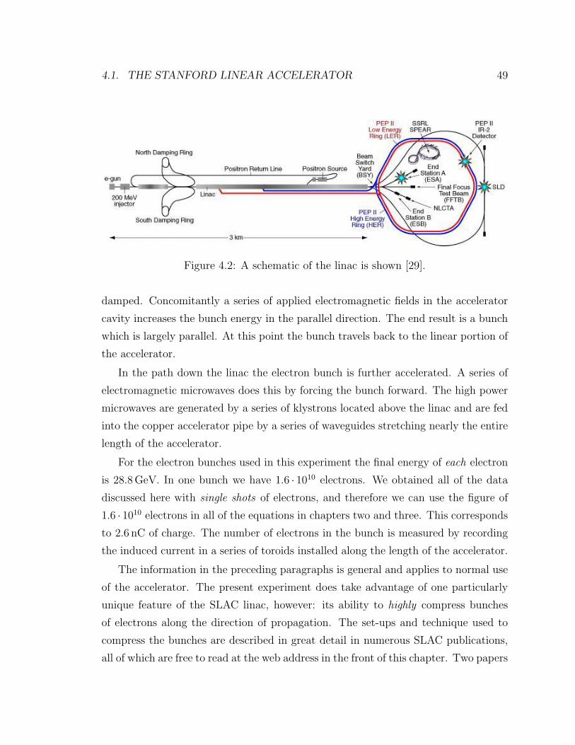
4.1. THE STANFORD LINEAR ACCELERATOR 49
Figure 4.2: A schematic of the linac is shown [29].
damped. Concomitantly a series of applied electromagnetic fields in the accelerator
cavity increases the bunch energy in the parallel direction. The end result is a bunch
which is largely parallel. At this point the bunch travels back to the linear portion of
the accelerator.
In the path down the linac the electron bunch is further accelerated. A series of
electromagnetic microwaves does this by forcing the bunch forward. The high power
microwaves are generated by a series of klystrons located above the linac and are fed
into the copper accelerator pipe by a series of waveguides stretching nearly the entire
length of the accelerator.
For the electron bunches used in this experiment the final energy of each electron
is 28.8 GeV. In one bunch we have 1.6 · 1010 electrons. We obtained all of the data
discussed here with single shots of electrons, and therefore we can use the figure of
1.6 · 1010 electrons in all of the equations in chapters two and three. This corresponds
to 2.6 nC of charge. The number of electrons in the bunch is measured by recording
the induced current in a series of toroids installed along the length of the accelerator.
The information in the preceding paragraphs is general and applies to normal use
of the accelerator. The present experiment does take advantage of one particularly
unique feature of the SLAC linac, however: its ability to highly compress bunches
of electrons along the direction of propagation. The set-ups and technique used to
compress the bunches are described in great detail in numerous SLAC publications,
all of which are free to read at the web address in the front of this chapter. Two papers

50 CHAPTER 4. EXPERIMENTAL SET-UP
in particular which provide insight into the process yet are still quite readable for a
non-accelerator physicist are [30] and [31]. Because the ability to expose the samples
in this experiment to pulses of two different temporal lengths is crucial, however, the
compression process is very briefly summarized here.
The compression takes place in three stages. The first stage is in a section of the
accelerator called the “Ring to Linac” (RTL) beamline compressor. It is composed of
a short radio frequency section with a series of bends which shorten the bunch from
roughly 6mm (or equivalently ∼ 20 ps) to roughly 0.5mm (1.7 ps). In this stage the
bunch is also further tuned to shape it for a more linear energy correlation in the
next accelerator section.
This next section is a new chicane, which is the specific instrument that enables the
extreme bunch compression. Physically, the chicane consists of four dipole magnets.
Each of them is 1.8 m long and has a field of 1.6 T. Prior to entering the chicane the
bunch is given an energy “chirp,” which is the accelerator physicists term for a cor-
related energy spread. In more transparent words, it means that as the bunch exists
in space, its different frequency (or equivalently energy) components have different
locations. Thus, the bunch has a time dependence of its instantaneous frequency at
one location. The spread comes from a combination of the wakefields in the linac and
an induced acceleration of the beam offset from the crest of the RF coming from the
klystrons. The first part of figure 4.3 illustrates what this means. After the chirp,
the energy spread σE/E0 is 1.6% rms and the bunch is ready to enter the chicane.
The chicane’s magnets serve the purpose of rotating the bunch in longitudinal space.
Here longitudinal space means time, or equivalently position, so a rotation in longi-
tudinal space means the spread of energy in time (position) changes. This process is
shown in parts (b) and (c) of figure 4.3 which illustrate this rotation process nicely.
In the above cited papers the final length of the bunch after the chicane compression
is 50µm (or 167 fs rms).
The final stage of bunch compression is in the actual beamline in the FFTB. This
beamline has sextupole magnets to chromatically correct for a small spot size, and
these magnets also very weakly further compress the bunch. The energy spread is
further reduced by the actual wakefield in the accelerator itself. For the compressed

4.1. THE STANFORD LINEAR ACCELERATOR 51
E-Field
Bending Magnets
Energy
Timeor
position
(a)
(b)
(c)
Figure 4.3: Part (a) shows the first stage of the compression process. The electronbunch is accelerated by the RF wave generated in the klystrons and the value of itsenergy varies with position. The graph shows this spatial variation, as the front ofthe bunch has an energy lower than that of the back. This is the generation of theenergy “chirp,” or spread, of the electron bunch. (b) shows the four bending magnetchicane which rotates the bunch by 90. This is accomplished because the higherenergy electrons in the back of the bunch have a shorter path length through themagnets than the lower energy electrons in the front of the bunch. (c) shows thebunch emerging from the chicane. Its length in longitudinal space is reduced, but theenergy spread has increased.

52 CHAPTER 4. EXPERIMENTAL SET-UP
bunches in this experiment the longitudinal spread is reduced to 21 µm (or 70 fs rms)
in this final compression stage. 20 µm is our spread in the transverse direction of the
bunch (the x-y plane cross section), making our final bunch almost spherical, rather
than ellipsoidal, in shape.
4.2 Experimental Set-up
All of the work utilizing the linear accelerator must be done in vacuum because
any particles in the beam pipe would lead to disastrous scattering of the electron
beam before any experiment could take place. Additionally, the plasma that would
be created by the ionized gas in the beamline would heat and damage the sample.
For this experiment the vacuum was on the order of 10−7 to 10−8 torr. We insert
a vacuum compatible six-way cross into the beamline. The location of the cross is
chosen such that it lies at the point of the tightest focus of the electron beam in the
FFTB tunnel. Two of the ports on the cross are attached to flanges on the linac
beampipe and permit the electron beam to enter and exit the cross. A third port is
used as an attachment for a baseplate to bolt the chamber to an optical table in the
FFTB tunnel and correspondingly fix the chamber at the appropriate height for the
beam to pass. Two ports have windows which allow us to see inside, and the final
port is used to attach the sample manipulator to the cross. A picture of the six-way
cross outside of the FFTB facility is shown in figure 4.4 (a).
We also use a vacuum compatible sample manipulator for the experiment. The
manipulator consists of a rigid arm inside a bellows and the accompanying motors to
move the arm to ensure correct placement of the samples with respect to the beam.
The manipulator has an Omniax translator with an XY table. We attached two
stepper motors to the translator to control the motion of the samples along the x
and y axes in our geometry. The stepper motors attached to the translator have
20,000 steps per revolution which means one full rotation moves the rigid arm 1mm
in the desired direction. These are the two degrees of freedom we need while doing
the experiment and, since the FFTB facility must be evacuated when the beam is
on for safety reasons, these two motors have to be controlled remotely. We use a

4.2. EXPERIMENTAL SET-UP 53
a b
Figure 4.4: The six-way cross which supports our sample manipulator is shown in(a). (b) shows the sample manipulator itself. When the experiment takes place themanipulator is rotated such that the bellows are on top. Within the vacuum-can seenon the left side of (b) is our sample fork, described below. This fork is inserted intothe six-way cross and the samples are thereby accessible to the beam.
Compumotor controller attached via an Ethernet cable to an outside computer to do
this. We interface with the controller by using a Labview program. We can also move
the rigid arm the the z direction of the experiment, but we set this position prior
to turning on the beam. Thus, this degree of freedom does not need to be remotely
controlled. It is driven by a screw which has 5 rotations per millimeter of movement.
A picture of the manipulator outside of the FFTB facility is shown in figure 4.4 (b).
In this picture the manipulator is horizontal, while during the actual experiment it
is vertical. The bellows on the right of the picture are at the top in the experimental
configuration.
The assembly of the six-way cross and the sample manipulator in the beamline at
the FFTB is shown in figure 4.5. Also visible in this picture are the motors, power
cables, and associated remote control cables.
Within the vacuum-can visible on the left side of figure 4.4 (b) is the fork which
holds our samples. A picture of this fork is shown in figure 4.6. The fork holds ten
1 cm by 1 cm samples at a time, as shown in the figure. The samples are held on the
fork by the curved metal fingers on the sides (they are yellow in the photo). These
fingers also serve the purpose of grounding the sample, which is essential to prevent

54 CHAPTER 4. EXPERIMENTAL SET-UP
Figure 4.5: The set-up of the six-way cross and sample manipulator in the FFTBbeamline is shown.

4.2. EXPERIMENTAL SET-UP 55
Figure 4.6: The sample fork, samples, grounded holding fingers, and wire scannersare shown. Each sample is 1 cm by 1 cm large.
its charging from any secondary electrons produced when the beam passes through it.
Additionally, the fingers hold the samples with the curved sides towards the sample
surface to avoid any sharp point contacts between the metal fingers and the metallic
samples.
Also visible on the left end of the fork are two sets of wire scanners. These wires
are used to determine the size of the beam in the x and y directions. The scanner
shown on the top (wires parallel to the vertical direction of the page) measure the
focus in the y direction and the scanner shown on the bottom (wires perpendicular
to the vertical direction of the page) measure the focus in the x direction. This is
accomplished by moving the scanners through the beam with the motor controllers.
When the beam is incident upon one of the wires, gamma rays are produced in
scattering events. These rays are subsequently detected several meters more down
the beamline. By moving the scanner in increments smaller than the width of the
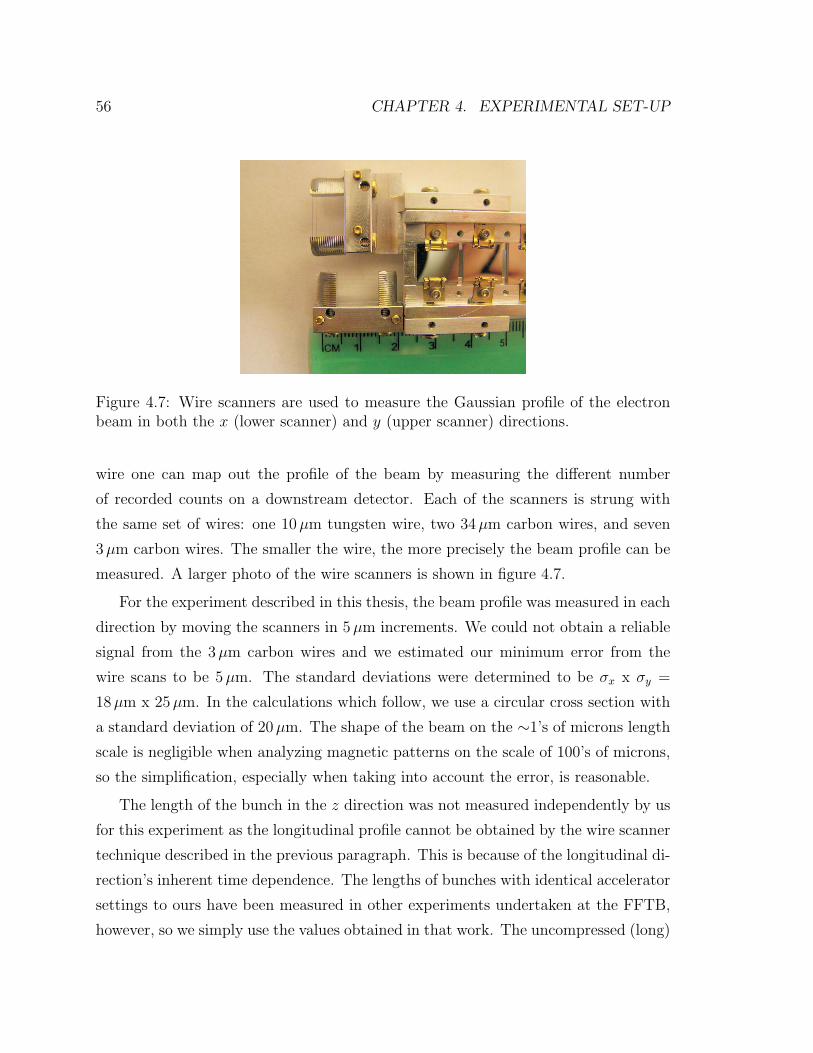
56 CHAPTER 4. EXPERIMENTAL SET-UP
Figure 4.7: Wire scanners are used to measure the Gaussian profile of the electronbeam in both the x (lower scanner) and y (upper scanner) directions.
wire one can map out the profile of the beam by measuring the different number
of recorded counts on a downstream detector. Each of the scanners is strung with
the same set of wires: one 10 µm tungsten wire, two 34 µm carbon wires, and seven
3µm carbon wires. The smaller the wire, the more precisely the beam profile can be
measured. A larger photo of the wire scanners is shown in figure 4.7.
For the experiment described in this thesis, the beam profile was measured in each
direction by moving the scanners in 5 µm increments. We could not obtain a reliable
signal from the 3µm carbon wires and we estimated our minimum error from the
wire scans to be 5 µm. The standard deviations were determined to be σx x σy =
18µm x 25µm. In the calculations which follow, we use a circular cross section with
a standard deviation of 20 µm. The shape of the beam on the ∼1’s of microns length
scale is negligible when analyzing magnetic patterns on the scale of 100’s of microns,
so the simplification, especially when taking into account the error, is reasonable.
The length of the bunch in the z direction was not measured independently by us
for this experiment as the longitudinal profile cannot be obtained by the wire scanner
technique described in the previous paragraph. This is because of the longitudinal di-
rection’s inherent time dependence. The lengths of bunches with identical accelerator
settings to ours have been measured in other experiments undertaken at the FFTB,
however, so we simply use the values obtained in that work. The uncompressed (long)

4.2. EXPERIMENTAL SET-UP 57
Figure 4.8: A head on view of the samples from the perspective of an electron beamtraveling down the beamline is shown. The beam impacts the sample at normalincidence, as discussed in chapter two.
bunch we use has a length of 690 µm which corresponds to a temporal length of 2.3 ps.
The compressed (short) bunch we use has a length of 21 µm which corresponds to a
temporal length of 70 fs.
In the final figure of this section, we show the sample fork actually inserted into
the six-way cross. Figure 4.8 shows the actual orientation of the experiment from the
perspective of the beam traveling down the beamline. This completes the mechanical
description of the experiment, and clarifies the cartoon schematic of the experiment
shown in figure 2.11
A note can be made about the actual steps taken during the exposure of the
samples. The experiment begins with the sample manipulator above the beam path.
The beam position stays fixed throughout the experiment, so the sample manipulator
is first lowered with the motors to measure the beam profile on the wire scanners. Here
we need to mention how we know where the beam is with respect to the sample fork.
We are actually blind to the position of the sample fork during the entire experiment
as there are no cameras inside the beampipe. Because of this we take a photograph
of the sample fork with all of the samples in place before we install everything at the
FFTB. Once everything is in place at the FFTB and the accelerator is on, we move
the sample fork with the LabView program in very small increments until we see

58 CHAPTER 4. EXPERIMENTAL SET-UP
counts on the downstream gamma ray detector generated by the beam hitting either
the wires or wire scanner mounts. We then continue these very small movements of
the beam over the wire scanners and their mounts until we are confident we know
exactly where the beam is with respect to the scanners. We also know exactly where
the scanners are with respect to the samples because of the photograph. Thus, after
the initial orientation we must keep track of where we are based on this initial point
and the distances on the photo.
After measuring the beam profile, the sample fork is aligned with respect to the
beam such that the beam passes directly below the left side of the bottom-most sample
on the manipulator. The experiment is done by first taking all of the short pulse
exposures by moving the manipulator arm down through the beam. The manipulator
arm is then moved over 3mm (to the left in figure 4.8) so the beam is aligned with the
right side of the samples. The accelerator is then tuned to the long bunch settings.
We then move the manipulator arm back up through the beam to take the long
bunch exposures. Thus, on the samples we have one line of exposures towards the
left side composed only of compressed bunch patterns and one line on the right of
uncompressed bunch patterns.
Mechanically the actual exposure (so not the initial alignment) is accomplished
by running a specific LabView program to automatically control the motors. For
measuring the beam profile we use the LabView program to simply move the motors
up and down and left and right as we need. When we actually expose the samples,
however, the accelerator runs at 1Hz and we thus use a LabView script to automat-
ically move the y axis motor in 1 mm steps also at 1Hz. Leaving a sample in the
path of the beam for longer than 1 sec would lead to multiple shots and destroy our
desired data. In practicality we only expose one sample at a time with the automated
LabView program and pause with the beam in the empty space between the samples.
This is done so we can make sure we are aligned on the edge of each sample before we
move it through the beam (for instance by moving over the very edge of the sample
to make sure we see downstream gamma ray counts).
After the exposures we can turn the beam off and re-enter the tunnel to remove
the samples. After the removal, we transport the samples in a magnetically shielded

4.3. ELECTROMAGNETIC FIELD OF AN ELECTRON BUNCH 59
desiccator to the SEMPA (SEM with Polarization Analysis) microscope facility to do
the imaging. The imaging process is described in the next chapter. We have extensive
experience showing that there is no damage of the patterns either in the transport or
in the imaging process.
Before closing the section, we can briefly mention the relative size scales of the
experiment. The samples are 1 cm x 1 cm. Our recorded patterns are ∼1mm by
0.5mm. The beam has a radius of 20 µm in the x-y plane. This means that the
beam is much smaller than the patterns and the patterns are much smaller than the
sample. Thus, on each sample we actually pass the beam through several times for
each pulse length. A typical number is ∼5 exposures of each length which means that
each sample would have 10 patterns total, separated by 3 mm in the x direction, as
explained above.
4.3 Electromagnetic Field of an Electron Bunch
The electron bunches used in this experiment are Gaussian in both space and time.
We will first consider the field profile generated by this bunch at locations outside
the bunch itself to develop an understanding of the general profile of the beam. At
distances outside the bunch cross section, the electromagnetic field profile is the same
as the profile of a current carrying wire, as the bunch of charged electrons traveling
down a vacuum pipe is analogous to a current flowing down a metallic wire. We can
thus write the magnetic field simply as [19]:
B(r, t) =µ0I(t)
2π r(4.1)
Including the Gaussian current profile yields:
B(r, t) =µ0Nee
(2π)3/2τ rexp
[t2
2τ 2
](4.2)
Here, τ is the standard deviation of the bunch in the z direction (time).
A complete description of the field must also, however, include the field profile
within the beam itself. At the very center of the bunch the field profile must go to

60 CHAPTER 4. EXPERIMENTAL SET-UP
zero as no electrons would be enclosed by an Amperian loop there. The field must
then rise as more and more electrons are included and contribute to the field. At large
r, an equation describing the field must recover the values given by equation 4.2. The
general equation describing the field created by our Gaussian distribution is: [19]:
B(r, t) =µ0Nee
(2π)3/2τr
[1− exp
(− r2
2σ2r
)]exp
[t2
2τ 2
](4.3)
Here, σr is the standard deviation of the bunch in the x− y plane. As stated in the
previous section, our σr =20µm.
The latter part of this thesis deals not only with the effects of ultrashort magnetic
fields on samples, but also the effects of ultrashort electric fields. Since the electric
field will be such an important quantity, we require an expression similar to equation
4.3 for the electric field as well. For pure electromagnetic fields the relationship
between B and E fields is simply:
B = (v × E)/c2 (4.4)
While the fields generated by the SLAC electron bunches are not pure electromagnetic
fields, the distinction is small, as discussed in detail in chapter eight. The near
indistinguishability arises because of the extreme relativistic factor, γ, of the bunch.
γ depends only on the energy of the electrons in the bunch which is the same for
our 28.8 GeV short and long pulses. 28.8GeV is equivalent to a γ factor of 5.64 · 104.
In practice this means that the fields of the bunch are highly compressed in the
longitudinal direction (as will be shown in the next section) giving them the pure
transverse profile of pure electromagnetic waves. Thus, for all practical purposes,
the bunch travels at the speed of light, c, and we can insert 4.3 into equation 4.4 to
describe the E field.
A plot of the peak magnitudes for the compressed τ =70 fs bunch and uncom-
pressed τ =2.3 ps bunch is shown in figure 4.9. The plot is obtained with equation
4.3 at t=0 (ie, it takes the peak of the Gaussian curve centered at t=0). The magni-
tudes are shown as a function of the distance away from the center of the beam, and
the fields are radially symmetric about the bunch. One can see from the figure that

4.3. ELECTROMAGNETIC FIELD OF AN ELECTRON BUNCH 61
0 100 200 300 400 500 6000
10
20
30
40
50
60
70
Distance (µm)
Mag
net
ic F
ield
(T
esla
)
Compressed vs. Uncompressed Bunch Field Strengths
0
0.5
1
1.5
2
x 1010
Electric F
ield (V
/m)
Compressed Bunch τ = 70 fs Uncompressed Bunch τ = 2.3 ps
Beam Parameters:
N = 1.6*1010
Energy = 28.8 GeVGamma = 5.6*104
σr = 20 µm
Figure 4.9: The peak field magnitudes for the compressed τ =70 fs bunch and uncom-pressed τ =2.3 ps bunch are shown as a function of distance away from the center ofthe beam. The peak electric and magnetic fields for the short bunch are 19.7GV/mand 65.9T respectively, while the peak fields for the long bunch are 0.6GV/m and1.98T.

62 CHAPTER 4. EXPERIMENTAL SET-UP
Magnetic Field Strength Values
average value104Exchange field
average value107Neutron Star
~ 10-6 seconds~103Pulsed coils
~ 10-13 seconds~102SLAC experiment
average value1Permanent magnets
minutes to hours~0.5Sun – spot
average value~ 5*10-3Sun – dipole field
average value~ 5*10-5Earth – dipole field
average value10-3Milky Way
milliseconds10-11Heart activity
milliseconds10-13Brain activity
Source of Field Strength (T) Duration
Electric Field Strength Values
constant108electrolyte (applied to a thin film)
1.3*1018Spontaneous pair production in ideal
vacuum (Schwinger pair production)
140 fs to 5 ps20*109SLAC experiment
107“Vacuum” breakdown (millitorr)
bunched strikes last ~ 500 ms
to 1 sec
106Lightning (in cloud, dry)
sometimes pulsed at µs to
avoid sample heating
106AlGaAs/GaAs quantum wells
average103Neutron star
strike is ~200 ms, usually 4
200 ms strikes per discharge
103lightning (cloud to ground)
constant1.4*1032 electrons, 1 µm apart
constant100 – 150Between the Ionosphere and the
Earth
constant1.4*10-92 electrons, 1 m apart
Source of Field Strength (V/m) Duration
Table 4.1: Sources, strengths, and durations of magnetic and electric fields are shown.The ultrafast and ultrastrong fields accessible with the SLAC compressed electronbunches are remarkable when compared to other experimental facilities, and enableus to study the effects of extreme conditions on magnetic materials.

4.4. RELATIVISTIC ELECTROMAGNETIC FIELD CONTRACTION 63
the maximum field strength is inversely proportional to the standard deviation of the
pulse width. As a result, it is not surprising that the ∼33 times shorter compressed
bunch has a peak field nearly 33 times stronger than the uncompressed bunch.
The peak fields shown in figure 4.9 are actually quite remarkable and not easily
accessible in either nature or other types of experimental facilities. To underscore
the impressive magnitude of the fields available at SLAC, table 4.1 shows ranges of
typical electric and magnetic field values from both natural and man-made sources.
Also included is the typical duration of the field when its value is appropriate. The
table clearly shows that the fields accessible with the compressed electron bunches at
SLAC are unique, and as a result they open up an exciting new realm of experiments
in high-field, ultrafast extreme conditions.
4.4 Relativistic Electromagnetic Field Contraction
The Lorentz transformations provide the relationship between space and time coor-
dinates in different inertial reference frames. The transformations rely on the fact
that the speed of light, c, is a constant independent of the motion of its own source.
For instances where objects or charges move slowly with respect to the speed of light,
the effects of the Lorentz transformations and special relativity can usually be safely
neglected. For the experiments described here, however, the speed of the electron
bunches is so close to the speed of light that a discussion of special relativity is neces-
sary. As stated in the previous section, the γ factor of the SLAC 28.8GeV electrons
is 5.64 · 104, where γ =1/√
1− (vc)2.
A full discussion of the role of special relativity in electrodynamics is quite beyond
the scope of this thesis. The goal of this section is simply to arrive at an expression
for the electromagnetic field of the SLAC relativistic electron bunch in the stationary
inertial frame of the observer (ie, us and the sample). We begin with the Lorentz
transformation equations to go from a stationary frame K to a frame K′moving at
some velocity v relative to K. For a detailed discussion of these equations, see [32],
chapter 11.

64 CHAPTER 4. EXPERIMENTAL SET-UP
x
xx
x
x
x
1
1
22
3 3’
’
’
r
vt q
P
angle = y
v
b
Figure 4.10: The inertial reference frames for the transformation of the electromag-netic field of a relativistic electron are shown. The electron of charge q is in frameK′which is moving to the right at velocity v with respect to K. It passes a station-
ary observer at point P in stationary frame K at time t=0. This figure follows thegeometry also used in reference [32].
E′
= γ(E + β × cB) − γ2
γ + 1β(β · E) (4.5)
B′
= γ(B − β × 1
cE) − γ2
γ + 1β(β · B) (4.6)
In the above equations β =v/c. For our problem of interest we are in the frame
K and consider a point charge q moving in a straight line path with a velocity v.
Supposing that the charge is moving in the positive x direction, the observer is at
point P , and the distance of closest approach between the observer and the charge is
b we have a geometry like that shown in figure 4.10.
We need to evaluate the E and B fields at point P . From the perspective of the
charge q the point P has coordinates x′1 = −vt, x
′2 = b, x
′3 = 0 and is at a distance
r′
=√
b2 + (vt′)2. Since r′is defined in the moving frame K
′we need to transform
it into our frame K. Because x1 = 0 for P in K we only need to transform t′
to

4.4. RELATIVISTIC ELECTROMAGNETIC FIELD CONTRACTION 65
accomplish this:
t′
= γ[t − (v/c2)x1] = γt (4.7)
We now need to write down the field components in the rest frame of the charge,
K′
so we can do the transformation of the fields into our frame K. Since q is not
moving in K′this is easy, and there are only two non-zero components of the E-field:
E′1 = − 1
4πε0qvt
′/r
′3 and E′2 = 1
4πε0qb/r
′3. Inserting the above expressions for t′and
r′yields:
E′1 = − 1
4πε0
qvtγ
(b2 + γ2v2t2)3/2(4.8)
E′2 =
1
4πε0
qb
(b2 + γ2v2t2)3/2(4.9)
Because we are going from the K′frame to the K frame, we actually require the
inverse of equations 4.5 and 4.6. This is also done in [32] and the only non-zero field
components are:
E1 = E′1 = − 1
4πε0
qvtγ
(b2 + γ2v2t2)3/2(4.10)
E2 = γE′2 =
1
4πε0
qbγ
(b2 + γ2v2t2)3/2(4.11)
B3 =1
cγβ E
′2 =
1
cβ E2 (4.12)
This formally completes our task of arriving at an expression for the fields in the
frame of an observer as a function of time. A more helpful way to visualize the fields,
however, is to take a snapshot of them in time and examine their spatial profile. By
algebraically eliminating b, v, and t from the above equations in favor of r and the
angle ψ (shown in figure 4.10), the E field as a function of the source charge’s present
position is [32]:
E =1
4πε0
qr
r3γ2(1 − β2 sin2 ψ)(3/2)(4.13)

66 CHAPTER 4. EXPERIMENTAL SET-UP
e-
Static Quasi-relativistic Ultra-relativistic
e-e-
Static Quasi-relativistic Ultra-relativistic
Figure 4.11: The spatial profile of the E field of an electron is shown for three cases.On the left is the spherically symmetric field of a stationary charge. In the center isthe profile of a charge moving at a velocity approaching c. The shape is contractedalong the direction of motion and enhanced in the direction transverse. In the ultra-relativistic limit, the field has become truly “pancake” like. The magnitude of thefield is enhanced by a factor of γ in the transverse direction and diminished by 1/γ2
in the direction parallel to the motion. In this case the E and B fields are nearlycompletely perpendicular to the direction of propagation of the charge and nearlycompletely perpendicular to each other.
From equation 4.13 we can see that the field is only isotropic when β =0, ie, when
the charge is not moving and we have a familiar spherically symmetric Coulomb field.
As soon as the charge starts to move, the field strength along the direction of motion
is scaled down by a factor of 1/γ2. This is in contrast to the direction transverse to
the direction of motion where the field is enhanced by a factor of γ. This scaling is
shown schematically in figure 4.11.
For our experiment’s γ the field is diminished by a factor of 3·10−10 in the lon-
gitudinal direction and enhanced by a factor of 5.6·104 in the transverse direction.
This is noteworthy because the longitudinal field component is virtually zero, which
is typically not a characteristic of electromagnetic fields generated by charge carriers.
It is, however, typically associated with pure electromagnetic fields propagating in
vacuum. Thus, for an observer located outside the radius of the bunch itself, it is
virtually impossible to distinguish if the field is coming from a charged particle or a
photon field. This indistinguishability between the charged particle field and a pure
photon field is a subject of chapter eight.

4.4. RELATIVISTIC ELECTROMAGNETIC FIELD CONTRACTION 67
Figure 4.12: (a) A Gaussian shaped electron bunch of 28GeV and indicated stan-dard deviations traverses a thin metallic ferromagnetic film perpendicular to the sur-face. (b) The E and B fields are confined to a flat disk perpendicular to the beamand lie entirely in the x − y plane. This is a portion of a figure originally con-tained in [33], copyright 2009 by the American Physical Society, original material:http://prl.aps.org/abstract/PRL/v102/i21/e217201
A final, summary, figure showing the overall experimental set-up and the complete
in-plane orientation of the electromagnetic field is shown in figure 4.12.

68 CHAPTER 4. EXPERIMENTAL SET-UP

Chapter 5
Experimental Results
This chapter begins with a description of the sample used in this experiment and
continues with a section on the microscopy technique utilized to obtain the magnetic
and topographic contrast images of the sample after exposure to the SLAC beam.
It concludes by showing both the magnetic contrast images and their topographic
counterparts. It is a relatively brief chapter, as the analysis and interpretation of the
data are the subjects of the rest of the text.
5.1 Sample Characterization
This experiment took place over the course of two runs in the FFTB facility. One of
these runs unfortunately experienced problems with the accelerator which prevented
us from obtaining the finely focused beam necessary to produce our patterns. The
remaining run was successful, and two samples from it yielded good quality magnetic
patterns from the femtosecond pulse exposures. One sample was a mixture of cobalt
and iron, and the other was pure cobalt. As discussed in chapter two, however,
the crucial point of this experiment is the comparison between patterns obtained
with femtosecond pulse exposures and patterns obtained with picosecond exposures.
Unfortunately, the pure cobalt sample did not have reliable picosecond data. Thus,
we have one cobalt-iron sample with good quality short and long pulse exposures.
Included in this chapter are femtosecond and picosecond data from that cobalt-iron
69

70 CHAPTER 5. EXPERIMENTAL RESULTS
sample.
The cobalt-iron metallic sample was fabricated by our collaborator Stuart S. P.
Parkin at IBM Almaden. It is a single crystalline uniaxial 10 nm thick ferromagnetic
film of Co70Fe30. It has a saturation magnetization at room temperature of M = 2T
corresponding to a shape anisotropy Ks = M2/(2µ0) = 1.59MJm−3, where µ0 is the
vacuum permeability. The sample has an in-plane uniaxial anisotropy energy density
of Ku = 0.076MJm−3. This is the energy density that must be overcome to switch.
The thin film is epitaxially deposited onto a 0.5mm thick [110]-MgO substrate with
intervening buffer layers consisting mainly of 30 nm Cr80Mg20. It is the [110]-MgO
substrate and buffer layers that give the sample its uniaxial anisotropy along the x
direction. The buffer layers also ensure a homogeneous deposition of the Co70Fe30
layer. Finally, the film is capped with a 1.5 nm thick layer of Pt to prevent corrosion.
5.2 Spin-Polarized Scanning Electron Microscopy
A complete analysis of our recorded magnetic patterns has two requirements. First,
we need a surface sensitive magnetic contrast technique to provide us with an image
of the alternating domain figure-eight pattern we anticipate. Second, we need a
topographically sensitive technique to provide us with an image of the actual sample
surface. Structural surface deformations can play a role in magnetic behavior and
also give us information about possible heating of the sample during exposure so the
condition of the surface must be observed.
The measurement technique we use to meet these two needs is spin-polarized
scanning electron microscopy. The technique is colloquially known as either spin-
SEM or SEMPA (for SEM with Polarization Analysis). As in conventional SEM
microscopy, a focused beam of high energy electrons is scanned across a sample. At
the sample surface the incident electrons are predominantly inelastically scattered
by the sample electrons, which causes a transfer of some of the incident energy to
the sample. The scattering often occurs more than once as the primary electron
continues to inelastically scatter and the newly excited sample electrons also scatter
off of, and in turn excite, more sample electrons. The end result is a cascade of excited

5.2. SPIN-POLARIZED SCANNING ELECTRON MICROSCOPY 71
secondary electrons. Many of these travel back to the surface and are ejected into
the vacuum chamber of the microscope. The angle at which they emerge depends on
the curvature of the sample surface. This is what gives the SEM the ability to image
sample topography [34].
If a ferromagnetic sample is excited by one of these high energy electron beams
the secondary electrons will be spin polarized [19]. The orientation of the spin is
preferentially in the opposite direction to that of the magnetization vector, because
of the negative sign of the electron (see equations 2.5 and 2.6). Thus, if one can
determine the orientation of the spin polarization, the direction of the magnetization
is simultaneously obtained. A conventional SEM, however, has no way to determine
the polarization state of the emitted electrons and they are all counted the same.
A SEMPA microscope is a SEM with a polarization analyzer in the detector which
provides a map of the magnetization. An illustration of the microscope is shown in
figure 5.1.
The number of SEMPA microscopes in use is significantly less than the number
of SEMs. In 2000 there were only eight microscopes in the world, and they differed
in the types of spin detectors they used and their ability to modify the sample during
measurement, ie to heat it, apply a magnetic field, etc [34]. The microscope we used
is run by our collaborator Dr. Rolf Allenspach at IBM Research, Zurich Research
Laboratory, Switzerland. His spin detector is of the Mott-type. Mott scattering is
described in detail in [19] and the references therein. We summarize the technique
below, however, and also provide the specifications for the microscope used to collect
our data.
The first step in the detection process is accelerating the beam of incident un-
polarized electrons and focusing it onto the sample. Choosing a beam energy is a
compromise between obtaining a high resolution and obtaining a high yield of polar-
ized secondary electrons. The best resolution is obtained at the highest beam energy,
which for our system is 25 keV. The polarized electron yield for metals, however,
peaks around ∼1-3 keV. In this energy range the polarization of the excited electrons
does not depend on the incoming beam energy and the collected electrons reflect the
spin imbalance in the energy bands. This lack of dependence occurs because the

72 CHAPTER 5. EXPERIMENTAL RESULTS
Incoming unpolarizedelectron beam
Polarizedsecondaryelectrons
Mottdetector
Figure 5.1: In spin-polarized scanning electron microscopy an unpolarized beam ofhigh energy electrons is incident upon a magnetic surface. The emitted secondaryelectrons are spin polarized and thus carry information about the magnetization of thesample. The electrons are collected in a detector with the ability to spatially separatethe spin states and count the electrons of each spin. From this information a map ofthe magnetization is obtained. A topographic image of the sample is simultaneouslyobtained by summing the counts on the two different spin detectors.

5.2. SPIN-POLARIZED SCANNING ELECTRON MICROSCOPY 73
electrons of interest come from the entire d-band. On their way to the surface all
of these electrons undergo so many multiple scattering events that the distinction
between electrons originating from the top and those from the bottom of the band is
lost. What is important is that the spin imbalance of the empty states in the sample
leads to different scattering probabilities for the spin up and spin down electrons as
they scatter towards the surface, and thereby enables us to probe the imbalance in
the bands. For this experiment we find a good compromise between resolution and
spin polarization at 5 keV.
In the first step one also needs to select an appropriate incoming beam size for
the incident electrons. The size depends on the apertures in the beam’s path to the
sample, and in choosing the size a compromise must again be made. Large apertures
enable one to obtain a lot of electrons and hence lead to shorter measuring times.
A large beam, however, means poorer resolution. In practice the best size one can
reasonably obtain and use is about 5 nm. For this experiment, however, ultrahigh
resolution was not a priority because we are imaging patterns 100’s of microns across.
Our final spot size was chosen with a high regard for collection efficiency and was
about 20 nm.
The resolution we obtain with our setup is determined by our image size and pixel
spacing. We take a field of view large enough to image the entire pattern at once.
This means our resolution is limited by our pixel to pixel distance, which is 1.8 µm.
This resolution is more than adequate to image our ∼1mmx0.5 mm patterns.
The second step is to collect the secondary electrons. In our microscope they
are transferred from the sample to the spin detector by a series of electron-optical
methods. They are first accelerated away from the sample with an energy of a few
hundred eV. Second they go through a deflector of 90 which is part of a cylindrical
mirror analyzer. The mirror analyzer selects the low energy electrons we are interested
in, where low means emitted from the sample with an energy less than ∼20 eV. Third,
the electrons are accelerated in stages to 3 keV, 12 keV, and finally 100 keV before they
are incident on the target of the Mott detector. All of these steps are tuned to collect
the largest possible angle of secondary electrons while still maintaining a good focus
of the beam on the detector.

74 CHAPTER 5. EXPERIMENTAL RESULTS
The third step is measuring the spin polarization, which is the step that uses the
Mott detector. In short, the Mott works by scattering the incident spin-polarized
electrons off of a thin target composed of heavy atoms. The target in our microscope
is a ∼100 nm thick gold foil. The scattering technique works to spatially separates the
two different spin states and then detect the two signals on two separated detectors.
In our microscope there are two pairs of detectors arranged in the same backward
scattering orientation shown in 5.1 (only one pair of detectors is shown in the figure).
The detectors are at ∼120 with respect to the forward direction. The angle is chosen
because this is the scattering angle at which the spin asymmetry is the highest. For
us, the first set of detectors measures the magnetization along the x axis and the
second set measures the magnetization component perpendicular to the surface. This
component for us is virtually zero as our sample is uniaxial, with the preferred axis
lying in the sample plane.
The Mott physically works as follows: When the high energy electrons are scat-
tered off of the gold they experience the intense Coulomb field of the heavy atom’s
positively charged nucleus. In the rest frame of the incident electron, this moving elec-
tric Coulomb field creates a magnetic field. The positive charge is moving towards
the electron in its frame, so from its perspective the magnetic field curls around
the positive nucleus in a counter-clockwise fashion. As the electron approaches this
inhomogeneous field, it will feel a magnetic force due to the gradient of the field.
This setup produces four possible scenarios. A magnetic moment up or a magnetic
moment down electron (corresponding to a spin down or up, respectively) could pass
to either the left or right of the scattering nucleus. To determine the behavior we
recall the force on a magnetic dipole in an inhomogeneous field is:
F = ∇(m · H) (5.1)
If a magnetic moment up electron passes to the right of the nucleus, m and H are
aligned, so equation 5.1 tells us the force on the electron will be in the direction of
the field gradient, so to the left. If a magnetic moment up electron passes to the left
of the nucleus, m and H are antiparallel, so the electron is forced in opposition to

5.2. SPIN-POLARIZED SCANNING ELECTRON MICROSCOPY 75
H
v
+
m
m
Figure 5.2: The concept of Mott scattering, as described in the text, is illustrated.There will be a force arising from the spin-orbit interaction as long as there is acomponent of m parallel or antiparallel to H.
the field gradient which is also to the left. Thus a magnetic moment up electron will
always be deflected to the left. By symmetry, the magnetic moment down electrons
will all be deflected to the right. An illustration of this is shown in figure 5.2.
In our microscope, the degree of spin polarization is determined by the difference
in the number of counts to the left and right in the Mott detector. The ability to
actually count single electrons is not, however, universal, and so the measurement of
asymmetry in the left and right detectors is given in terms of current. The expression
is normalized and defined as:

76 CHAPTER 5. EXPERIMENTAL RESULTS
A =Iright − Ileft
Iright + Ileft
(5.2)
This normalization ability gives spin-polarized scanning electron microscopy a sig-
nificant advantage over other magnetic contrast imaging techniques. The advantage
comes about because the normalization removes the effect of fluctuations of the incom-
ing beam current and emitted secondary electrons. This is confirmed by the analysis
of magnetic images and their simultaneously obtained topographic counterparts (the
topographic image is obtained by summing the electrons collected in the counters).
Features visible in the topographic images do not appear in the magnetic images,
thus making the magnetic contrast images truly pure magnetic information. [34].
Using the SEMPA technique is not, however, without challenges and the effect
arising from the magnetic moment interacting with the magnetic field of the scattering
nucleus is not the only effect to which the incoming electrons are subject. Namely
the effect of normal Rutherford scattering is still present, and it heavily influences the
trajectory of the electrons. Thinking back to the description of the Mott technique,
the Coulomb field responsible for Rutherford scattering will pull the incoming electron
in the opposite direction to that dictated by its spin orientation 50% of the time.
Ultimately, the difference in counts between the two polarization states is quite small
and the entire detection scheme is of relatively low efficiency.
There is a formal way to calculate how strong a spin asymmetry function is for a
spin polarized beam incident on a particular kind of target which takes into account
the effect of Rutherford scattering. The calculation is based in atomic physics and it
gives you the difference in signal current, A, you would expect purely from the spin
polarization of the secondary electrons, P , on your two detectors. The inputs to the
calculation are the characteristics of the target, the incoming energy of the beam,
and the angle of the detectors with respect to the incoming beam. The output of the
calculation is known as the Sherman function, S [19]:
A = S P (5.3)
Here, P is normalized, just as A:

5.3. EXPERIMENTAL DATA 77
P =N ↑ −N ↓N ↑ + N ↓ (5.4)
Ideally, one would think that a 100% spin polarized beam would yield a 100%
spin asymmetry on the detectors. In actuality, the asymmetry is around 0.2. For
the SEMPA system we used, the Sherman function value is 0.22. This means, for
instance, if we have a incoming beam of 200 electrons polarized at P =+/-20% we
would count 109 electrons in one detector and 91 in the other.
Now that we understand how the images are obtained, we are prepared to look at
them.
5.3 Experimental Data
We first show two magnetic contrast images from the Co70Fe30 sample in figure 5.3.
The only difference between the experimental conditions present when pattern
(a) of figure 5.3 was created from those of pattern (b) is the temporal length of
the bunch. Part (a) shows an image resulting from the τ =2.3 ps bunch and part
(b) shows an image resulting from the τ =70 fs bunch. The patterns were created
on the same sample, the short and long bunches had identical numbers of electrons
(Ne =1.6·1010), and the field of view for both images is the same (902 µm x 451µm).
Following the logic presented in this thesis until this point would lead us to predict
that these patterns should be the same, but as one can see they are markedly different
(even after taking into account the deviations from ideal behavior discussed in chapter
three). There are three primary differences in the patterns and we can begin the
discussion about them by stating that the picosecond pattern has the characteristics,
both magnetically and topographically, that we would predict. The magnetic pattern
looks like a (largely) symmetric figure-eight, and the topographic pattern, which is
shown later in this section, displays a small area of damage where the beam passed
through it. Upon a cursory examination of the femtosecond data, however, one can
see that neither the magnetic pattern nor the topographic condition of the sample is
what we would anticipate.

78 CHAPTER 5. EXPERIMENTAL RESULTS
a
b
100 µm
M
Figure 5.3: Two magnetic contrast images are shown. Part (a) shows an imageresulting from the τ =2.3 ps bunch and part (b) shows an image resulting from theτ =70 fs bunch. The direction of premagnetization is to the left, as shown. The fieldof view for both images is the same: 902 µmx 451µm. Both exposure are from thesame Co70Fe30 sample described in the first section of this chapter. Both exposureswere also made with beams containing identical numbers of electrons: Ne =1.6·1010.According to the calculations carried out in chapters two and three, the patternsshould be identical, but they are obviously not. Discrepancies still exist even aftertaking into account the deviations from ideal behavior discussed in chapter three. Part(b) of this figure originally appeared in [33], copyright 2009 by the American PhysicalSociety, original material: http://prl.aps.org/abstract/PRL/v102/i21/e217201

5.3. EXPERIMENTAL DATA 79
100 µm
Figure 5.4: Two circles are superimposed on the femtosecond data to illustrate themagnitude of the up-down asymmetry in the pattern. Our theory predicts the patternshould be fit by circles and be symmetric.
The first magnetic difference is a pronounced spatial asymmetry present in the
femtosecond pattern but not in the picosecond. The picosecond pattern is symmetric
from top to bottom, as predicted by the calculations in chapter two. The femtosecond
pattern is not. There is a remarkable flattening of the femtosecond pattern
on the top extending out at an angle of ∼+/- 45 from the origin about the
+y axis. There is no obvious reason why this up-down asymmetry on the
femtosecond pattern should exist. This same flattening was observed on the the
pure cobalt sample mentioned in the beginning of this chapter. In order to illustrate
the difference between the recorded femtosecond shape and the expected circular one,
two circles are superimposed on the pattern in figure 5.4
The second magnetic discrepancy is a pronounced difference in the domain be-
havior at the center of the patterns. The picosecond pattern exhibits stripe domains,
while the femtosecond pattern does not. The presence of the domains indicate that
the sample heated above its Curie point, Tc =1200 K, over the region where the do-
mains are visible. This region extends ∼100µm away from the beam impact site. The

80 CHAPTER 5. EXPERIMENTAL RESULTS
heating destroyed the magnetic information encoded in the sample by the pulse, and,
long after the pulse had passed, the sample cooled and re-magnetized with the stripe
domain pattern. A similar destruction of magnetic data is also visible in figure 3.2.
We will discuss at length later why this heating is not surprising with the picosec-
ond pulse but the lack of any observable heating effects in the femtosecond
image is unexpected and requires an explanation.
Here we should also note that while the picosecond pattern is largely symmetric
from left to right, the symmetry is not perfect. We are not confident as to the source of
this asymmetry, but similar distortions appeared in other picosecond patterns formed
on this same sample. Three possible explanations have been considered, but more
experiments are needed to draw any conclusions. First, the asymmetric distortion
could be the result of a slightly off center elliptical beam. The effect of elliptical beam
shapes has been explored as a possible solution to the asymmetry in the femtosecond
patterns and this work shows that distortions of the beam will manifest themselves
as left-right distortions of the pattern. Second, the effect might arise because of a
slight variation of material properties across the film within a few percent. This is,
however, unlikely as the same distortion is observed on patterns spatially separated.
Third, the distortion could be the result of the metal fingers holding the sample to the
fork as shown in figure 4.6. Due to experimental constraints, this pattern was taken
quite close to the right edge of the 1 cmx 1 cm sample, and hence close to the fingers.
We know that secondary electrons are created when the beam passes through the
samples, and this process is discussed in the following chapters. The purpose of the
metal fingers is to ground the samples so they do not remain statically charged after
the beam has passed. A static discharge may have occurred at the metal finger by
the right side of the picosecond pattern and disturbed the predicted behavior. This
is also, however, unlikely as the distortion is visible on patterns with varying distance
to the fingers.
The topographic images simultaneously obtained with the magnetic contrast im-
ages are shown in figure 5.5.
The right panels in figure 5.5 appear to reveal that the beam has left visible
damage in the picosecond bunch exposure while the femtosecond one is remarkably

5.3. EXPERIMENTAL DATA 81
100 mm
Picosecond Images
Femtosecond Images
Figure 5.5: Since topographic images of samples exhibiting magnetic contrast are noteasy to immediately orient oneself on, magnetic images are shown on the left of thefigure to provide a point of reference. The top row of the figure shows the picoseconddata and the bottom the femtosecond. All images are the same size and scale. Thepicosecond topographic image reveals a small area of ablation and/or change in thework function of the sample roughly equal to the size of the beam, while there is notopographic modification caused by the femtosecond pulse.

82 CHAPTER 5. EXPERIMENTAL RESULTS
100 mm10 mm
Figure 5.6: The figure shows a zoomed topographic image of the picosecond exposure.The portion of the magnetic contrast image enclosed in the box is the portion shownin the zoomed topographic image on the right. The zoomed image confirms that therehas been either a small ablation of the surface and/or a change in the work functionof the atoms at the surface where the bunch passed. There is no similar alterationvisible on the femtosecond exposure.
damage free. To obtain a clearer picture of the alteration of the sample where the
picosecond length bunch passed we show a second set of further zoomed images in
figure 5.6.
We believe we ablated ∼1 monolayer of the sample where the picosecond length
bunch passed, but strictly speaking we cannot give an exact number for the level of
ablation in the sample. This is because what is visible in the microscope image is
actually a combination of topographic and chemical contrast. The source of the chem-
ical contrast is that the maximum intensity and the shape of the secondary electron
spectrum depends on the material under investigation. This comes primarily from

5.3. EXPERIMENTAL DATA 83
the difference in work functions of different materials. Thus, what we can strictly
say is that we have either ablated the material in the beam impact spot, changed it
from its surroundings significantly enough to alter its work function, or accomplished
some combination thereof. There is no similar alteration, however, visible in the fem-
tosecond data. Why the femtosecond pattern remains topographically or chemically
unmarked by the beam is not immediately obvious, but we can conjecture that the
source of the damage is most likely connected with the same effects which produced
the heating of the sample as well.
To summarize, before looking at the data we would assume that patterns created
by either picosecond or femtosecond duration pulses would be identical (or at least
predictable after taking into account the deviations from ideal behavior discussed in
chapter three) as long as the number of electrons used to create each pattern is the
same. When we look at the data created by pulses which are identical in every aspect
except for their temporal duration, however, we find this is not the case (even after
taking the chapter three considerations into account). Two primary differences exist:
1. The picosecond pattern fits the expected circular shape of our calculations, while
the femtosecond pattern is markedly flattened in its upper portion.
2. The picosecond pattern heats above the Curie point in a region ∼100µm around
the beam impact site. The femtosecond pattern does not heat above Tc. Addition-
ally, the picosecond pattern has a small area of ablation and/or chemical change at
the point of beam impact.
Over the next three chapters we will discuss the sources of these differences. These
explanations form the bulk of the thesis work.

84 CHAPTER 5. EXPERIMENTAL RESULTS

Chapter 6
Electric Field Induced
Magnetoelectronic Anisotropy
In chapter five we showed the magnetic contrast images from the picosecond and
femtosecond length electron bunch exposures and noted that a primary difference
between the images is that the picosecond exposure fits the expected circular shape
while the femtosecond exposure is markedly flattened in its upper portion. In this
chapter we discuss the source of this difference. The following two chapters will
discuss the heating and damage anomalies.
In short, the flattening of the femtosecond pattern is due to a new type of transient
all electric field induced magnetic anisotropy in our thin film metallic ferromagnet.
The strong (∼ 109 V/m) and short (τ =70 fs) electric field pulse created by the fem-
tosecond electron bunch creates the anisotropy and, hence, it is only present during
the passage of the pulse. Generating an anisotropy in this way is truly unique as the
electric field is strong enough to distort the valence charge distribution of the metal,
yet too brief to alter any of the atomic positions. The work discussed here is the first
observation of a pure electronic structure alteration generating such an anisotropy in
a metallic ferromagnet.
While this magnetoelectronic anisotropy is present it strongly influences the mag-
netization dynamics of our sample and, since it is the record of the dynamics which is
85

86CHAPTER 6. ELECTRIC FIELD INDUCED MAGNETOELECTRONIC ANISOTROPY
ultimately captured in the final switching pattern, we have a diagnostic tool to qual-
ify and quantify the anisotropy’s effects. The fact that the record of the all electric
field induced anisotropy is present immediately indicates that its magnitude rivals
that of the magnetic field of the beam of tens of tesla, which is already a remarkable
observation.
Before we begin the detailed explanation of the observations it is useful to note
that while electric fields have been used to manipulate magnetization before [35–37],
there has yet to be a demonstration of a technique which utilizes only an external
electric field to actually switch the magnetization. The experiments and ideas detailed
in this thesis and also published in [33] and [38] provide the first clear path towards
an all electric field induced switching mechanism viable for normal ferromagnetic thin
film metals at room temperature. This, in some respects, is one of the primary goals
of modern magnetism research as it is not only of fundamental interest, but also of
practical importance as an all electric field switching mechanism could usher in a new
generation of binary magnetic recording devices.
6.1 Manipulating Magnetic Anisotropy
As discussed in chapter two, the magnetic anisotropy energy of a system is the energy
it takes to move the magnetization of the system from its easy to its hard axis. It is
typically quoted in terms of an energy density and the units we use in this thesis are
MJm−3, as employed in chapter five when we described the inherent shape and uni-
axial anisotropy of our Co70Fe30 sample. Magnetic behavior in general is determined
by three competing anisotropies determined by shape, internal strain, and crystal-
lographic structure of the sample. When magnetic anisotropy is determined by the
crystalline structure of the magnetic material, it is done so via the bonding configu-
ration. An anisotropic ligand field creates anisotropic orbits for the electrons making
up the solid, and this anisotropic bonding configuration influences the preferred ori-
entation of the magnetization through the spin-orbit interaction. For a thorough
discussion of magnetocrystalline anisotropy see [19].
If one wants to manipulate the magnetic anisotropy, an immediately obvious way

6.1. MANIPULATING MAGNETIC ANISOTROPY 87
to do so is thus to change the bonding configuration of the solid by changing the
position of the atoms. By creating a new atomic arrangement with a different orbital
overlap pattern on adjacent lattice sites one changes the orbits of the electrons and,
again through the spin-orbit interaction, the magnetic anisotropy. An example of this
scheme of manipulation is shown in figure 6.1.
Compress
Figure 6.1: One possible method of manipulating magnetic anisotropy is shown. Thebonding configuration on the left has a preferred axis for the magnetization along thevertical direction of the page. If the structure is compressed, for example, the physicalbonding lengths and potentially the orientation of the orbitals are altered and thisrearrangement affects the spin system through the spin-orbit interaction. After thecompression the new favored energetic minimum for the magnetization is along theaxis horizontal to the page.
A second and perhaps not as immediately obvious way to manipulate the anisotropy
is to leave the atomic positions unchanged and strictly alter the electronic orbits of
the electrons of the atoms. This could be accomplished through the application of a
strong electric field, where “strong” means of a magnitude rivaling that of the ligand
field. For the type of magnetic solid used here, the ligand field is on the order of
1V per atomic spacing, or equivalently ∼10V/nm ∼10GV/m. This type of manip-
ulation is shown in figure 6.2 assuming the presence of a unipolar pulse, like that of
the SLAC beam. A similar manipulation could be accomplished with a bipolar field
pulse where the orientation of the valence electron cloud distortion changes by 180
halfway through the pulse.
While changing either the atomic positions of a magnetic system or its valence
electron distribution will potentially change the magnetic anisotropy of the solid,

88CHAPTER 6. ELECTRIC FIELD INDUCED MAGNETOELECTRONIC ANISOTROPY
Electric
Field
Figure 6.2: A second possible method of manipulating magnetic anisotropy is shownhere. The atomic cores are represented by the black dots and the electronic valencecharge distribution by the pink clouds. The electronic configuration on the left ofthe figure gives an anisotropy axis along the vertical direction of the page. If oneapplies an electric field to the atoms which rivals the strength of the ligand fieldand is only present as a pulse with a temporal width comparable to the timescale ofelectronic motion one can solely change the valence charge distribution of the system.This redistribution of charge, but not atoms as the pulse is too short, will be felt bythe spin system through the spin-orbit interaction and hence can ultimately affectthe preferred orientation of the magnetization. In this illustrative example the newpreferred orientation is horizontal to the page.
the timescales over which each of these methods can produce an effect differ greatly
and this needs to be considered to correctly interpret our experimental results. If
one wants to move the atoms in a crystal they are limited by the phonon frequencies
supported by the crystal. These frequencies typically correspond to atomic motion on
picosecond timescales. The femtosecond duration field pulse which we pass through
our sample is thus approximately two orders of magnitude faster than the shortest
typical disturbance which can propagate through a crystal lattice and the atoms
simply cannot respond to it. A pure electronic distortion of valence electron orbits,
however, is not limited by the supported phonon modes, and the orbiting electrons
of a magnetic system can respond to a pure electric field distortion on the timescale
of the distortion, here in the 100’s of femtoseconds.

6.2. QUALITATIVE DATA ANALYSIS 89
6.2 Qualitative Data Analysis
The previous section outlined the two basic requirements for inducing a magnetoelec-
tronic anisotropy with a pure electric field:
1. One needs an electric field with a magnitude comparable to the ligand field of the
solid. Here, this is equivalent to ∼10GV/m.
2. One needs this field to have a duration short enough such that the atomic positions
remain unchanged so only the valence electronic orbits are distorted.
The characteristics of the femtosecond length SLAC electron pulses are in line
with both of these above requirements. However, the challenge is actually inserting
this electric field into a metallic ferromagnetic sample. Here, we have a unique set
of circumstances that allow us to circumvent this usual hurdle. As discussed in the
final section of chapter four, while a stationary electron has a spherically symmetric
Coulomb field, an electron moving with relativistic speeds experiences a field compres-
sion so that the field is a flat radially symmetric sheet perpendicular to the direction
of motion. Similarly, a bunch of relativistic electrons will have a field perpendicular
to the beam direction. When such a normally incident bunch traverses a thin metal
film the large electric field of the bunch is simply inserted into the metal film with
the boundary condition E‖out = E
‖in [19, 32, 33]. The same logic also tell us that no
screening of the bunch field can take place prior to the electrons’ arrival at the sample
surface because the magnitude of the field is all in the transverse component. It is
the longitudinal component which could potentially generate an image charge in the
sample prior to the bunch’s arrival and here that component is absent. In short, the
entire magnitude of the electric field is in the parallel component, it is this component
which is inserted into the metal, and none of the field has been pre-screened before
its arrival at the sample surface.
These points are crucial to the experiment, as if we were not able to insert this
ultrastrong, ultrafast field pulse into our sample it would be impossible to distort the
valence states of the electrons and manipulate the magnetism. Combining this with
the fact that the 10 nm thickness of the film is smaller than the material’s skin depth

90CHAPTER 6. ELECTRIC FIELD INDUCED MAGNETOELECTRONIC ANISOTROPY
of ∼50 nm, we know that the strong electric and magnetic fields are both present
inside the sample [33].
After we are assured that we do have strong fields inside our sample, we can
progress onto studying the effects that these fields produce. To interpret the pattern
recorded in our sample by the femtosecond bunch it is necessary to separate effects
generated by the B field from those induced by the E field. The behavior of the
magnetization under the influence of the B field has already been extensively discussed
in chapters two and three so we can move directly to a discussion of the E field
induced behavior. Before continuing it is helpful to note that all of the dynamics
which will be discussed here take place during the passage of the τ = σt = 70 fs
pulse, as the electric field induced effect is a purely transient phenomenon which
exists only while the pulse is present. While the electric field only directly affects the
magnetization during the pulse, we will show that the effects produced during this
time subsequently determine the course of the dynamics after the pulse has passed,
while the magnetization is settling in the internal anisotropy fields of the sample. This
is identical to the case of the dynamics induced by the magnetic field of the pulse in
the three-step model, as the beam field excites the magnetization out of the plane
and after the pulse has passed the moments precess purely in the internal anisotropy
fields.
Before introducing an explicit model for the behavior of the magnetization dynam-
ics in the strong electric field, it is helpful to discuss a “toy” picture for the electric
field induced effect. In this way we can develop a full qualitative understanding of
what the electric field can potentially do, and this will in turn greatly facilitate the
quantitative analysis of the data later in the chapter. For our toy picture we will start
by showing the two possible orientations for the preferred anisotropy axis created by
the electric field. Prior to an examination of the experimental data we do not know
which of these two possible orientations will be the one ultimately actualized. We will
then discuss how each of these possible anisotropy axes can be looked at as creating
an effective magnetic field for the magnetization of the sample while it is present.
The relation of the anisotropy axis to an effective magnetic field is a key step in
the qualitative analysis of the data because as soon as an effective field exists the

6.2. QUALITATIVE DATA ANALYSIS 91
magnetization will precess around it in a relatively simple way. We can thus see how
the magnetization would precess for each of the two possible cases and subsequently
how this precession will influence the following relaxation of the magnetization in
the internal anisotropy fields. By comparing the results of this qualitative exercise
to the experimental data, we will see we can determine the actual orientation of the
anisotropy axis created by the electric field during the femtosecond pulse.
To develop our toy model we first use the fact that the electric field can create
only a preferred axis for the magnetization, not a direction. Symmetry considerations
tell us that these preferred axes can be either along the axes defined by the electric
field lines or perpendicular to them, but from pure symmetry considerations alone we
cannot deduce which of these will be the preferred configuration. Figure 6.3 shows
the two possible orientations for the anisotropy axes created by the electric field. On
the left is the case where the electric field creates an easy axis, meaning that the
magnetization will want to align along the electric field lines. On the right is the case
where the electric field creates a hard axis, meaning that the magnetization will want
to align perpendicular to the electric field lines. The geometry in the figure is set up
such that it exactly reproduces the experimental conditions. The figure is looking at
the plane of the sample and the electron bunch would be propagating into the page.
The center of the coordinate system represents the location at which the bunch passes
through the sample and the electric field lines point towards this point of impact as
shown in figure 4.12.
When an anisotropy axis exists it provides a preferred axis for the magnetization
to align with, and by combining the orientation of this axis with the direction of the
magnetization we can move to a picture where the anisotropy creates an effective
magnetic field. Then, just like in any other field, the magnetization will precess. This
correspondence between an anisotropy axis and an effective magnetic field is discussed
in section 2.4 and is quite important because as soon as we have a magnetic field we
can predict the character of the dynamics of the magnetization in that field. The
important distinction is that, in contrast to the anisotropy axis, the effective field will
have a direction given by the projection of the magnetization onto the axis at any
point. Taking this last consideration, we can modify figure 6.3 to include the direction

92CHAPTER 6. ELECTRIC FIELD INDUCED MAGNETOELECTRONIC ANISOTROPY
x
y
Case 1: E field createsan easy axis - preferred
orientation is along E
Case 2: E field createsa hard axis - preferred
orientation isperpendicular to E
x
y
x
y
Figure 6.3: The figure shows the two possible configurations for the easy axis createdby the electric field. The geometry shown is that of the actual experiment - theelectron bunch would propagate into the page at the center of the coordinate systemand its associated electric field lines would point towards the origin. In case 1 theelectric field creates an easy axis along the electric field lines. This easy axis isrepresented by the pink arrows in each quadrant. In case 2 the electric field createsa hard axis, with an easy axis correspondingly perpendicular to the field line. Thisperpendicular configuration for the easy axis is again shown by the pink arrows ineach quadrant.
of the initial magnetization and associated projection of that magnetization onto the
proposed easy axes in each quadrant. This gives us the direction of the effective field,
Heff . This projection is shown in figure 6.4.
After determining the direction of the effective magnetic field in each quadrant we
can determine the direction of the associated torque on the magnetization and corre-
spondingly what dynamics will follow. As an example we will take case 1, quadrant
1. Equation 2.3 tells us that the torque on M from Heff will be out of the page in
the +z direction and equation 2.7 tells us that the associated movement of the mag-
netization will be into the page in the −z direction. We can do this same exercise for
all of the quadrants for each of the two cases to determine whether the magnetization
in each quadrant will move either in to or out of the page. These results are shown
in figure 6.5.

6.2. QUALITATIVE DATA ANALYSIS 93
x
y
Initial Orientation of M
Case 1: E field createsan easy axis
Case 2: E field createsa hard axis
x
y
x
y
Heff
Heff
Heff
Heff
Heff
Heff
Heff
Heff
Figure 6.4: The black arrows show the direction of the premagnetization along the−x direction in each quadrant. When the strong electric field is present during thefemtosecond pulse the anisotropy axis it induces creates an effective magnetic field,Heff , in which the magnetization will precess. The orientation of Heff is given by theprojection of the magnetization onto the anisotropy axis. This projection is shown forboth possible cases in all four quadrants by the orange dotted line and the associatedeffective field by the orange arrow.
While at this point we still do not know whether case 1 or case 2 is the experi-
mentally realized situation, we have exhausted the information which we can gather
from looking at the electric field induced effect alone. To determine whether the E
field creates an easy or hard axis we have to also use the information we have about
the B field induced effect. We go about this by looking at the torque and motion of
the magnetization under the influence of the B field of the pulse and combining this
with the information we have about the torque/motion induced by the E field for
each of the two cases in each of the four quadrants. We do this because we want to
see whether the motions induced by the E and B fields are in the same or opposite
directions in each quadrant. If the torques/motions add to each other we know that
the magnetization will have a larger out of plane angle with respect to the sample
plane than it would have if only the B field had acted upon it. This, in turn, means
that the magnetization has more energy after the pulse passes and thus can precess
through a larger angle before settling along one direction of the easy axis in step

94CHAPTER 6. ELECTRIC FIELD INDUCED MAGNETOELECTRONIC ANISOTROPY
x
y
Initial Orientation of M
Case 1: E field createsan easy axis
Case 2: E field createsa hard axis
x
y
x
y
Heff
Heff
Heff
Heff
Heff
Heff
Heff
Heff
Motion of inM Heff
Out of page
Into page
Into page
Out of page
Into page
Into page
Out of page
Out of page
Figure 6.5: As soon as the direction of Heff is determined for each quadrant in eachof the two cases one can easily determine the direction of the induced torque andassociated movement of the magnetization in the field. Here these directions aregiven for each quadrant where motion out of the page corresponds to a movementin the +z direction and motion into the page corresponds to a movement in the −zdirection.
two of the three-step model introduced in chapter two. In this situation it becomes
“easier” for the magnetization to switch. If the torques/motions subtract from each
other, however, the magnetization will have a smaller out of plane angle with respect
to the sample plane than it would have if only the B field had acted upon it. This,
in turn, means the magnetization has less energy and will correspondingly precess
through a smaller angle before settling along one direction of the easy axis. In this
situation it becomes “harder” for the magnetization to switch. Figure 6.6 shows the
motion of M induced in each quadrant by the B field of the electron pulse and figure
6.7 shows the appropriate addition or subtraction of the motions in each quadrant
for the two possible cases.
From simply looking at the addition and subtraction information provided in the
bottom right portion of figure 6.7 we can immediately see that the electric field creates
an easy axis for the magnetization while it is present. A look back at figure 5.4 shows
that in the upper part of the figure an ideal circular switching pattern would have a

6.2. QUALITATIVE DATA ANALYSIS 95
x
y
x
yMotion of inM B
Initial Orientation of M
Into page
Into page Out of page
Out of page
Figure 6.6: Using the same principles as we did to arrive at the direction of motionfor M under the influence of the effective field induced by the electric field we canarrive at the direction of motion induced by the pure B field of the SLAC pulse. Herethe direction of premagnetization is still shown by the black arrows and the directionof the B field is shown in blue for each quadrant. The resultant motion is againindicated by the words.

96CHAPTER 6. ELECTRIC FIELD INDUCED MAGNETOELECTRONIC ANISOTROPY
Magnetization
B field
E field inducedeffective field
Initial orientation of M
Motion of inM B
Do and field inducedmotions add to or
subtract from each other?
B E
Case 1: E field createsan easy axis
Heff
Heff
Heff
Heff
Out of page
Into page
Into page
Out of page
Case 2: E field createsa hard axis
Heff
Heff
Heff
Heff
Into page
Into page
Out of page
Out of page
AddAdd
AddAdd
SubtractSubtract
SubtractSubtract
Motion of M in Heff
x
y
x
y
Initial Orientation of M
Into page
Into page Out of page
Out of page
Figure 6.7: Here we undertake a completely qualitative exercise where we determinewhether the motions induced independently by the E and B fields add to or subtractfrom each other for our two possible cases of E field induced behavior. The columnon the right represents this combination and we can immediately see after comparingthis column to the experimental data that the electric field does in fact create an easyaxis for the magnetization while it is present.

6.3. SYMMETRY CONSIDERATIONS AND SIMPLE MODELING 97
switched (black) domain extending up to the boundary of the superimposed circle.
This is a region of moments which “should” have switched under the influence of a
magnetic field, but do not when the magnetic field dynamics are considered with the
additional electric field induced ones. This means that the moments in this region
effectively absorbed less energy than they would have under the sole influence of the
B field; ie, the motions subtracted from each other. This subtraction in the upper
part of the pattern will only exist if the electric field has created an easy axis, as
shown in figure 6.7. Thus, the E field must create an easy, rather than a hard, axis.
We should also note that the circles in figure 5.4 are only to guide the eye. What
they slightly obscure (and what our fits will show) is that the magnetization does
in fact switch at a larger radius in quadrants 3 and 4 than it would be expected to
under only the B field influence. Thus, the torques/motions are in fact enhancing
each other in the lower part of the pattern.
6.3 Symmetry Considerations and Simple Model-
ing
Before delving into a full quantitative analysis of our data we can make one more,
still largely qualitative, observation about the symmetry of the electric field induced
effect. By looking at figure 6.5 we can see immediately that the effect has a four
fold symmetry pattern which is distinctly different from the two fold, figure-eight
like symmetry induced by the magnetic field torque. Figure 6.8 shows two Matlab
plots which illustrate this point. We know what the equitorque/equienergy deposition
lines created by the magnetic field will look like by use of equations 2.27 and 2.28.
Sample lines are shown in grayscale on the left side of the figure calculated using the
maximum magnetic field value obtained during the pulse, ie the figure is a snapshot
of what the torques would look like at one point during the pulse. Here, white
represents a torque into the page (or motion out of the page) and black represents a
torque out of the page (or motion into the page). We also know this torque will fall
off like 1/r2. Prior to a quantitative analysis we do not know what the strength of

98CHAPTER 6. ELECTRIC FIELD INDUCED MAGNETOELECTRONIC ANISOTROPY
Magnetic Field Electric Field
Figure 6.8: The characteristics of the torques on the magnetization induced by theB (left) and E (right) fields are shown. The magnetic field torque falls off as 1/r2
while the electric field torque falls off as 1/r3 because the effect must go as E2, asdiscussed in the text. Here, white represents a torque into the page (or equivalentlymotion out of the page) and black represents a torque out of the page (or equivalentlymotion into the page). Since we do not know the strength of the electric field inducedeffect without a full quantitative analysis, an arbitrary scaling factor has been usedwith respect to the magnetic field torque to make the magnitude of the electric fieldtorque reasonable over the scope of the plot.
the electric field induced torque is. What we do know, however, is that because the
effect must go as E2 (because the E field provides only the preferred axis and not the
preferred direction), the torque the effect induces will fall off like 1/r3. We also know
the angular dependance of the torque by taking the projection of the magnetization
onto the electric field vector at each point. We use this information and an arbitrary
scaling factor with respect to the magnetic field to make the torques reasonable over
the scope of the plot to arrive at the plot shown on the right of figure 6.8. For the
plot on the right side white again represents a torque into the page and black out of
the page.
We can take this analysis one step further to arrive at a rough fit for the first switch
of the pattern with the inclusion of the electric field effect. This is accomplished by
tuning the arbitrary factor mentioned in the preceding paragraph to arrive at a value
for the electric field torque and adding (or subtracting) this to the value for the
magnetic field torque over the scope of the pattern. The arbitrary factor is tuned
until the overall shape of the actual data is reproduced. Figure 6.9 shows the data
with two fits superimposed upon it. The blue line shows what the expected first

6.3. SYMMETRY CONSIDERATIONS AND SIMPLE MODELING 99
switch outline would look like with only the influence of the magnetic field and the
red shows what the expected first switch outline looks like with the combined influence
of the magnetic and electric fields. Both of these outlines were plotted on the same
coordinate system, which means that the downward shift of outline including the
electric field effect is in fact real. The detraction of energy in quadrants 1 and 2 is
clearly visible as is the enhancement of the switching in quadrants 3 and 4. While
figure 6.9 reproduces fully the qualitative features of the first switch, any quantitative
information we could garner from it is slightly opaque as we have used this arbitrary
scaling factor. A rigorous quantitative analysis is undertaken in the next section and
a very nice order of magnitude calculation is presented in the section after that which
enables us to arrive at a good estimate for the strength of the electric field effect in
terms of energy density.
Figure 6.9: The figure shows two equitorque/equienergy deposition outlines selectedto match the first switch of the pattern. The blue line shows where the first switchwould lie if only the B field were influencing the dynamics. The red dots show themodified outline of the first switch including the E field induced magnetic anisotropy.A good agreement with the outer switching boundary is achieved, as explained inthe text. Both plots are on the same coordinate system with the same origin so theflattening of the pattern on the top and the enhancement of the switching on thebottom are in fact genuine.

100CHAPTER 6. ELECTRIC FIELD INDUCED MAGNETOELECTRONIC ANISOTROPY
6.4 Quantitative Data Analysis
Now that we have a solid qualitative picture of what to expect for the behavior of the
electric field induced magnetoelectronic anisotropy we can undertake a more rigorous
quantitative approach. Before presenting the results we should note that, apart from
the flattening at the top of the pattern, there are three other departures from the ideal
circular shape visible. First, the domains close to the point of impact between the two
ring systems are asymmetric. This is most likely due to magnetic aftereffects, such
as the migration of a domain wall [39]. Also present is a small left-right asymmetry
which can be attributed to a bunch with a slightly elliptical cross section. Finally, a
blurring of the boundary between switched and un-switched regions is observed due
to the formation of zig-zag domain walls, as noted in previous work [15, 22]. These
effects are not related to the electric field induced magnetoelectronic anisotropy, and
so do not play a role in the remainder of the discussion.
As stated in the first part of this chapter, the E field does not act on the magneti-
zation directly but can modify the charge distribution and then affect the magnetism
through the spin-orbit coupling. The expansion of such an E field induced anisotropy
energy density EE must only contain even exponents to satisfy the symmetry require-
ments and has the general form
EE = ε0 + KE = ε0 − ε2 cos2 ϕ− ... (6.1)
where ε0 is isotropic and ϕ is the angle enclosed by E and M. KE is the anisotropic
spin-orbit energy density created by the E-field distortion of the orbits. For our
definition, KE ≤ 0 and ε2 ≥ 0 [33]. The sign of KE here assumes EE is at a minimum
when M is aligned parallel with E, as we found to be the case in the previous section.
If the perpendicular orientation were the favored one, fitting our experimental data
to equation 6.1 would simply produce reversed signs for the constants.
As in our toy model, the creation of a new E field induced anisotropy axis generates
a torque on M. This torque has a magnitude:
|TE| = |∂EE/∂ϕ| = |2ε2 sin ϕ cos ϕ| (6.2)

6.4. QUANTITATIVE DATA ANALYSIS 101
and it acts on M as long as the E field is present, hence its aforementioned transient
nature.
Like the torque on the magnetization due to the B field, TE causes M to move out
of the plane of the film by an angle which varies with the distance r from the beam
center and the angle of E with M. We do not, however, know a priori what effect
this new torque will have, so we use the same approach as with the toy model and
say that since we know what pattern a B field alone produces, we can observe any
variations from the expected pattern to elucidate the effect of the transient anisotropy
introduced by E [33].
To illustrate how this is accomplished quantitatively we show three simulated
patterns in figure 6.10. All three patterns are calculated with the LLG equation
discussed in chapter two and in [19]. Simulation (a) is calculated with the regular
LLG equation including only the torque from the B field and with a damping constant
α = 0.015. This is the same simulation procedure as used in [15, 27]. Simulation (a)
also includes the aforementioned precession in the sample’s anisotropy fields during
the pulse [27]. This simulation can account solely for the width of the outermost two
black rings. Both the total number of rings and the overall shape are incorrect [33].
Thus, we modify our simulation to try to adequately reproduce the data.
The first modification we make is due to the fact that the LLG equation in its
original form does not account for spin wave instabilities occurring in the large angle
precession of M about the demagnetizing field after the field pulse. This effect was
introduced in chapter three and is discussed in detail in [22,23,26]. Reference [26] in-
cludes a much more detailed treatment of the subject and shows that in the equation
of motion for magnetization precession the precession is always unstable and is ac-
companied by a growing spin wave instability, as was also mentioned in the discussion
in chapter three. Here, we will summarize the important points for this experiment
and provide the parameters used in our model.
The feedback effect of spin waves on the precession of the uniform mode can be
described in terms of a Gilbert damping constant which depends on the state of the
spin wave modes which grow exponentially with time. In slightly plainer language, in
the large angle excitation regime the probability is high for the uniform precessional

102CHAPTER 6. ELECTRIC FIELD INDUCED MAGNETOELECTRONIC ANISOTROPY
Figure 6.10: The figure shows three magnetic patterns calculated with the Landau-Lifshitz-Gilbert equation. Part (a) assumes that only a B field is inside the sample andthat the damping of the precession is constant in time. Part (b) also only uses the Bfield but includes a damping factor which increases exponentially with time to accountfor spin wave instabilities. Part (c) includes the time dependent damping and both theB and E field effects. Pattern (c) reproduces the main features of the experiment.This figure originally appeared in [33], copyright 2009 by the American PhysicalSociety, original material: http://prl.aps.org/abstract/PRL/v102/i21/e217201

6.4. QUANTITATIVE DATA ANALYSIS 103
mode to fracture into multiple higher order spin wave modes. The effects of this
fracture on the magnetization dynamics can be incorporated into a LLG equation
analysis by modifying the usual constant Gilbert damping parameter, α, so that it
varies depending on the spin wave modes present and their temporal evolution. In
practicality, these higher order modes work to return the system to an equilibrium
position faster than the uniform mode would and thus effectively increase the damp-
ing. This is the same behavior shown in chapter three, figure 3.3. We also show a
similar plot to 3.3 for this experiment in figure 6.11 where the exponential increase in
damping is again clear as the precession time (or equivalently total precession angle)
increases.
As also first mentioned in chapter three, our collaborator Alexander Kashuba (who
is also the author of [26]) models the spin wave instability for this experiment by a
local Gilbert constant αin(t, ~r) that grows exponentially with time, t, according to:
dαin/dt = γ|M z(t, ~r)/M0|αin(t, ~r). This comes from the second term of equation 3.8
and γ is still the dimensionless increment of the instability. The instability growth
rate is proportional to the local precession frequency in the field HD ∼ M z(t, ~r) about
the sample normal- hence, no precession means no instability growth, as one would
intuitively expect. The integration constant is determined according to Fermi’s golden
rule for the probability to excite a spin wave in second order perturbation. The total
dissipation term is the sum of the intrinsic and the instability terms: α(t) = α0+αin(t)
(again, from equation 3.8). The parameters used in the simulation of patterns (b)
and (c) in figure 6.10 are g = 2, Ku/Ks = 0.041, γ = 1.46, and the intrinsic Gilbert
dissipation constant α0 = 0.017. As one final remark about the spin wave instabilities,
we note that the instabilities develop on a time scale ≥ 100 ps, that is long after the
bunch has passed. These dynamics thus take place after the generation of the electric
field induced anisotropy. Their inclusion accounts for the observed number of rings
and their variable widths [33].
Simulation (b) does not, however, capture the deviation of the pattern from a
circular shape. This can only be obtained if one also considers the effect of the E
field according to equation 6.1. A simulation including TE and assuming the parallel
configuration between E and M is favored is shown in figure 6.10 (c). It shows TE

104CHAPTER 6. ELECTRIC FIELD INDUCED MAGNETOELECTRONIC ANISOTROPY
0 20 40 60 80 100 120 140 1601
2
3
4
5
6
7
Precession Time (ps)
Sw
itch
ing
En
erg
y (E
/Ku)
Switching Energy vs Total Precession Time For the 140 Femtosecond Length Pulse
Left side of the patternRight side of the pattern
Figure 6.11: A plot of the total switching energy (scaled by the uniaxial anisotropyenergy density) vs. switching time is shown for both the left and right sides of theswitching pattern. The damping increases as one enters the large angle of precessionregime due to the exponential growth of spin wave instabilities. The growth of theseinstabilities is included in the simulations of our data in parts (b) and (c) of 6.10. Theslight discrepancy between the left and right sides of the pattern could be attributedto a slightly asymmetric beam, as mentioned in the text.

6.4. QUANTITATIVE DATA ANALYSIS 105
is opposed to the torque TH in the upper part of the pattern and adds to it in the
lower part, which matches the observations. This shows the induced anisotropy axis
is indeed parallel to E, as we anticipated from our toy model. The deviation of the
experimental pattern from the circular shape is thus direct evidence for the existence
of a transient anisotropy inside the metallic sample during the field pulse [33].
To quantify the transient anisotropy energy density KE in equation 6.1 from the
experimental pattern we investigated various approximations. We obtain the best
fit of the data by representing the transient anisotropy as a series expansion of the
Legendre spherical harmonics about the direction of the E field. We retain only L = 2
and L = 4 harmonics in our model:
KE = −ε2(E) cos2 ϕ− ε4(E) cos4 ϕ (6.3)
We approximate the two transient anisotropies (the easy-axis and the fourth-order)
by two rational functions:
ε2(E) = E0(b2E2 + c2E4)
(1 + E4)(6.4)
and
ε4(E) = E0b4E4
(1 + E4)(6.5)
Here b2, c2, b4 are adjustable parameters of the model, and the anisotropy energy
density E0 = ME0/µ0c and normalized field E = E/E0 account for that fact that
ε2(E) and ε4(E) saturate near the bunch. In our best fit: b2 = 0.74, c2 = 0.78,
b4 = 0.41 and E0 = E(r = 120 µm) [33].
Here is an ideal point at which to reinforce the enormity of this electric field in-
duced magnetoelectronic anisotropy. As mentioned in the start of the chapter, before
doing any calculation we know that the value of the energy density induced by the
electric field must be appreciable because we can see its effects in the recorded pattern,
meaning the effect rivals that produced by the magnetic field of tens of tesla. This
fit, however, corresponds to a time-averaged saturation anisotropy around 40MJm−3
which is not only large but, to our knowledge, is the largest magnetic anisotropy

106CHAPTER 6. ELECTRIC FIELD INDUCED MAGNETOELECTRONIC ANISOTROPY
observed so far in a magnetic metal. It is significantly larger than the static mag-
netic anisotropy energy density of 17MJm−3 of hexagonal SmCo5 [40] and larger
anisotropies have so far been observed only for isolated Co atoms and clusters on a
Pt(111) surface [41] [33].
The reason why this electric field induced effect is not observable in the picosec-
ond length exposure or in any other previous work utilizing the SLAC electron beam
is also now quite evident. This effect scales predominantly as E2 and the picosec-
ond bunch’s electric field is ∼33 times weaker than the femtosecond’s. This means
that the anisotropy generated by the electric field of the picosecond length bunch is
∼1089 times weaker than that created by the femtosecond bunch, and thus completely
obscured by the dynamics induced by the magnetic field.
6.5 Quantitative Analysis - Estimation Method
We used the first portion of this chapter to develop a qualitative understanding of
the magnetoelectronic anisotropy and the second portion to describe a more rigorous
mathematical model. In this section we approach a middle ground and introduce
a “by hand” calculation method to arrive at the correct order of magnitude of the
electric field induced anisotropy for the first switch. The technique is limited to the
first switch because it is not sophisticated enough to account for the energy lost to
the damping of the precession, and for the first switch the influence of damping is
negligible. The key idea will be that we can use the previously understood behavior of
the magnetic field effect to calibrate the scale of the dynamics induced by the electric
field effect. The approach is somewhat graphical and uses the principles described in
chapter two section six and chapter three section two.
We will limit our discussion to the dynamics in the first quadrant, as the same
technique can be applied anywhere across the scope of the pattern. We will also take
the same geometry as the actual experiment with a sample premagnetized along the
−x direction. Since the spirit of the approach is to use the magnetic field effects to
scale the electric field ones, we begin by drawing the outline of the first switch which
we would expect if we had only magnetic field induced switching. This is simply

6.5. QUANTITATIVE ANALYSIS - ESTIMATION METHOD 107
a semicircle. We know, however, that in the first quadrant with a sample initially
magnetized along −x the torques created by the magnetic and electric fields oppose
each other, and thus that the actual first switching boundary will fall inside this
semicircle. For simplicity, we take just one line drawn out at 30 to the +x axis
and will concentrate on the dynamics along it. Knowing that the torques subtract,
we make a point on the 30 line which represents a possible location of the outer
boundary of the first switch when the electric field plays a role. This sketch, with
letters assigned to key points, is shown in figure 6.12
x
y
B
C
A
Figure 6.12: The figure shows the expected semicircular outer switching boundary oneobtains if only the magnetic field influences the magnetization dynamics. We know,however, that when the electric field plays a role in the first quadrant the resultingtorques work to pull the magnetization in opposite directions and effectively make itharder for the moments to switch. This results in a switching boundary at a smallerradius than we would have if the magnetic field acted alone. We concentrate on thedynamics along one line, which we have selected to be at 30 to the +x axis. Threeimportant points are marked on the figure: A denotes the location of the intersectionbetween the circular switching boundary and our line, B denotes the intersectionof this same boundary with the x axis, and C denotes a possible location of theoutermost switching boundary when the electric field plays a role.
We need to take a moment to discuss the significance of some of the points in figure
6.12, specifically the distance between points A and C as this distance represents the
amount of torque effectively “taken away” by the electric field effect. We know that
some minimum amount of torque must be exerted on a magnetic moment for it to
precess out of the plane enough to ultimately switch. Correspondingly, the equitorque

108CHAPTER 6. ELECTRIC FIELD INDUCED MAGNETOELECTRONIC ANISOTROPY
line represented by the outermost switching boundary always represents the moments
on which just enough torque has been exerted such that they can eventually overcome
the uniaxial anisotropy energy density and switch. When only the B field effect is
present, this torque has been provided solely by the B field. When the E field
effectively takes torque away from the amount bestowed by the B field, this first line
is still an equitorque line equivalent to the amount of torque required to switch once,
but it now has a smaller radius corresponding to the vector sum of the torques from
the B and E fields. This smaller radius corresponds to a higher B field value required
to switch because the E field has effectively detracted torque.
We can now devise a method to quantify the strength of the E field effect. While
we do not know a priori what shape the switching pattern generated with the influence
of the E field will be, we do know that a set of data recorded under the influence of a
strong E field will pass through a point similar to C and the exact point indicated by
B. We know the first switching boundary would pass through B because the electric
field will not have an influence on the magnetization dynamics when the direction of
the field is either parallel or antiparallel to the initial direction of M. This means that
along the x axis no E field induced effects are observable, and the pattern develops
solely under the influence of the B field. The derivation hinges on the fact that from
the inherent anisotropies of a sample (Ku and Ks) and the knowledge of how much
angular precession a moment at any point on the sample will be subjected to from the
application of the B field, we can find the angle through which the E field has caused
the moment to precess. Since we know the length of the pulse which has created this
anisotropy we can find the (average) effective magnetic field required to induce such
a precession (here we will make the simplification of a square field pulse in lieu of
the actual Gaussian shape used in the experiment). This effective field can then be
related to an energy density.
As the first step in the derivation, we draw a semicircle on our sketch which passes
through the origin, point C and a point on the +x axis, which we label D. Recalling
that the lines of equitorque exerted by the magnetic field are circles, we can use the
location of the intersection between this semicircle and the x axis to find the magnetic
field’s contribution to the switching at point C. The modified sketch is shown in figure

6.5. QUANTITATIVE ANALYSIS - ESTIMATION METHOD 109
6.13
x
y
BD
C
A
Figure 6.13: The figure shows a semicircle passing through C and the x axis. Thisis a line of equitorque (and so also equienergy deposition) for the magnetic field.Finding the magnetic contribution to the switching at point D therefore also tells usthe contribution at point C. Since we also know what angle of elevation it takes toswitch once, if we know point C lies on the outer most switching boundary we canultimately find the energetic contribution of the magnetoelectronic anisotropy.
We continue by using the expression for the angle of elevation required to switch
once from the discussion in chapter three section two.
αswitch = sin−1
(√Ku
Ku + Ks
)(6.6)
To switch, αswitch must be equal to the angle of precession induced by the B field
minus the angle of precession induced by the E field, because the induced torques
subtract from each other in the upper part of the pattern. This enables us to write:
αswitch = αB − αE (6.7)
Where αB and αE are the angles induced by the B and E field torques respectively.
We already have an expression for αB in terms of experimental parameters (chapter
two section six):
αB =e2 Nµ0
me2π
x
r2(6.8)

110CHAPTER 6. ELECTRIC FIELD INDUCED MAGNETOELECTRONIC ANISOTROPY
This enables us to write an expression for αE:
αE =e2 Nµ0
me2π
x
r2− sin−1
(√Ku
Ku + Ks
)(6.9)
Here we should be careful to note that x and r represent locations with respect to
point C or D. This is because we want to find the contribution from the magnetic field
to the total torque where the moments have actually switched, and this contribution
is the same at C and D because they lie on the same semicircle. It will be the
difference between this magnetic field contribution and the angle actually required to
switch that is attributed to the electric field induced effect.
To ultimately obtain the desired expression for an energy density we need to use
αE in an expression for the effective magnetic field generated by the E field. We can
do this because we know that the entire angle of precession αE was passed through
while the electric field was present inside the sample, ie over a time roughly equal to
2σt. We then simply have an angular frequency of
ωE =αE
2σt
(6.10)
This can be related to an effective (time averaged) magnetic field:
ωE =eµ0 HE,eff
me
(6.11)
Combining the above two equations yields:
HE,eff =αE me
2σt e µ0
(6.12)
This expression can then be directly related to an expression for the anisotropy energy
density induced by the E field, KE
HE,eff =2 KE
Mcos(ϕ) (6.13)
Where ϕ is the angle between the magnetization and its projection onto the easy axis
created by the E field, here this is 30. This finally yields:

6.6. ON ALL ELECTRIC FIELD INDUCED MAGNETIC SWITCHING 111
KE =αE me M
2σt eµ0 2 cos(ϕ)(6.14)
KE =
(e2 Nµ0
me2πxr2 − sin−1
(√Ku
Ku + Ks
))me M
2σt eµ0 2 cos(ϕ)(6.15)
We will now use this expression with some reasonable numbers to arrive at an
actual value for an electric field induced magnetic anisotropy energy density. Taking
the location of point D as 200·10−6 m from the origin (to solve the problem you
need either the location of point D or the coordinates of point C, we take D), e as
1.602·10−19 C, N as 1.6·1010, µ0 as 4π · 10−7 mkg/(s2A2), me as 9.11·10−31 kg, Ku as
0.076MJ/m3, Ks as 1.59MJ/m3, M as 2T, and 2σ as 140 · 10−15 sec, we arrive at:
KE = 8.79 MJm−3 (6.16)
The value of 8.79MJm−3 arrived at here is already large, and, since this is the
value at a distance of ∼200µm from the center of the pattern and the energy density
increases as E2, we know that closer to the center the effect will be much stronger.
As discussed in the previous section, fits to the actual data show a saturation of the
magnetoelectronic anisotropy energy density at about 40MJm−3 at E fields higher
than∼7.3 GV/m, which is the largest magnetic anisotropy ever observed in a magnetic
metal.
6.6 On All Electric Field Induced Magnetic Switch-
ing
In today’s modern storage devices magnetic bits are switched by the application of a
magnetic field generated by current flow through wires. These coils are often bulky,
however, and the Ohmic heating they generate provides a major pathway for energetic
loss. An additional drawback to magnetic field switching techniques is that the write
time for data is currently limited to about 1 bit per nanosecond due to inductive effects

112CHAPTER 6. ELECTRIC FIELD INDUCED MAGNETOELECTRONIC ANISOTROPY
in the wires used to generate the fields. An all electric field switching technique could
potentially improve data storage capabilities in all of these areas as one would only
need to apply an electric field instead of a current and, as demonstrated through this
experiment, electric field induced effects can manipulate the magnetization on the
femtosecond, rather than the nanosecond, timescale.
Using an electric field to induce magnetic switching is not, however, completely
straightforward. The reason is rooted in the same symmetry property discussed
in this chapter which enables the electric field to create only a preferred axis for
the magnetization and not a direction. Thinking back to the technique we used to
determine the direction of the effective magnetic field created by the electric field, one
can easily see that the direction of the magnetization could never be moved through
an angle greater than 90 by the application of a pure electric field. Thus, one needs
to use some sort of trick if they want to actually switch the magnetization through
180 without applying an additional external magnetic field.
The necessary trick is that demonstrated through the work in this thesis. What we
have shown here is that it is possible to use the electric field to create a preferred axis
for the magnetization, and that the effective magnetic field simultaneously created in
this process will cause the magnetization to precess into an excited state with respect
to the internal anisotropy fields of the sample. Thus, we need to use the electric field
only to put the magnetization into an excited state which will later deterministically
decay into the switched configuration [38]. This emphasizes the point that in this
experiment we do not use any external fields to actually switch. Both the applied
magnetic and electric fields generated by the SLAC electron bunch act to excite the
magnetization, but it is always the demagnetization field created by the internal
anisotropy fields which actually does the switching. We need the external fields to
simply prepare the magnetization into a state from which its decay is deterministic.
It is this trick of letting the demagnetization field actually switch the magnetization
that lets us overcome the symmetry problem. It is this same trick which also enables
us to potentially push the writing time of bits with an electric field technique down
into the femtosecond regime, as the external electric field only needs to be applied
long enough to put the magnetization in the appropriate excited state. In this sense

6.6. ON ALL ELECTRIC FIELD INDUCED MAGNETIC SWITCHING 113
the writing time is distinctly different from the switching time, and it is only the
write time which is actually important for technological applications [38].
While the data presented in this thesis shows a hybrid switching technique in
which both the magnetic and electric fields play a role in exciting the magnetization
out of the plane of the sample, the fundamental demonstration of the feasibility of
an all electric field induced switching technique is clear. This is because the only
criterion for switching is the induction of a sufficient in-plane anisotropy density KE,
so that the associated torque rotates M out-of-plane by a sufficient angle during
the pulse such that it can later precess around the demagnetization field across the
hard in-plane axis [38]. As long as the electric field is strong enough to create a
sufficient anisotropy through the spin-orbit coupling and the field is applied for a short
enough time such that only the valence orbital are disturbed, all electric field induced
switching should be possible. The concept of all electric field induced switching is
not limited, however, to the valence electron distortion technique discussed here.
Using the concepts from the beginning of the chapter we arrived at the idea of a
picosecond duration manipulation of the atomic positions in a magnetic crystal also
altering the magnetic anisotropy. A sufficiently strong voltage pulse could accomplish
this and thus provide a second pathway to all electric field induced switching [38].
This could most likely be accomplished on a picosecond timescale with a ferroelectric
material [38].
We have one final interesting point to address, which moves the discussion away
from the unipolar pulses used here. Since the anisotropy energy is an even function of
E, mostly ∝ E2, it should be possible to use a linearly polarized photon pulse instead
of the DC pulse used here to switch. This technique has the advantage that the
linear B field effects will cancel over a full wave cycle, thereby opening the possibility
for true all electric field control of the magnetization of a normal metal at room
temperature. Using such a method would, however, require that one have a source
with an appropriate frequency. This frequency has two requirements: First, one needs
an oscillation time on the scale of electron dynamics, and second one needs to avoid
exciting interband transitions which would lead to potentially catastrophic heating of
the magnetic material. Conveniently, a source in the low terahertz meets both of these

114CHAPTER 6. ELECTRIC FIELD INDUCED MAGNETOELECTRONIC ANISOTROPY
requirements. Inconveniently, however, no tabletop terahertz source currently exists
which also has an electric field approaching the required GV/m regime. Thus, for
the present, a true demonstration of pure all electric field induced magnetic switching
remains elusive.

Chapter 7
Single Electron Energy Loss
Mechanisms
7.0.1 Motivation for Consideration of the Heating Problem
At this point our magnetic deformation problem is solved, and so the first question
at the center of the thesis is also resolved. What remains then, is to determine why
the picosecond bunch heats the sample at the point of impact while the femtosecond
one does not. The next two chapters will deal with this effect.
Before we begin, however, we need to emphasize the true importance of this
problem in the context of the rest of the experiment. At a first glance it might
seem that the magnetic problem and the heating problem are disconnected from each
other, when in actuality they are not. In the previous chapter we showed that our
sample absorbs an enormous amount of energy from the incident field pulse, as it is
not trivial to induce the strong distortion of the valence electron orbitals which we
observed. After the magnetic effect has been induced, the important question then
becomes how do we get that energy out of the system before the sample is destroyed?
Also, to truly begin at the beginning, how exactly did the sample actually absorb the
energy in the first place?
We know that in the femtosecond pulse case the sample absorbs energy and is
able to expel enough of it to not have it leave any trace of its presence (outside of the
115

116 CHAPTER 7. SINGLE ELECTRON ENERGY LOSS MECHANISMS
recorded magnetic effects). We know that in the picosecond pulse case, even though
the sample has heated to the Curie Point, it did survive the pulse which means either
the sample did not absorb an appreciable amount of energy or there was also some
dissipation channel present for it. In this way, the magnetic problem and the heating
problem are inextricably linked.
In these next two chapters we explore the heating problem with the above in mind.
In this chapter we discuss the interactions which take place between the individual
electrons making up the electron bunches and the sample to see if they provide any
insight to the absorption question or to our discrepancy between the short and long
pulse heating effects. In the next chapter we treat the collective effects of the total
electrons’ fields on the sample.
7.0.2 Framing of the Energy Loss Problem
When a high energy electron beam passes through solid matter it will lose a portion
of its incident energy. The interactions which govern the amount of energy lost
are numerous and their analysis is complicated by the inherent statistical nature of
the problem. For example, if one were to project a focused monoenergetic beam of
electrons at a thin target, the beam would emerge with a distribution of energies
and trajectories because each electron experiences a unique path, associated energy
loss, and corresponding deflection as a result of the different probabilities associated
with each interaction. This statistical process is important for the present experiment
because interactions between high energy electrons and our sample could potentially
contribute to the observed damage with the picosecond exposure.
The problem and discussion are immediately complicated, however, by the fact
that none of the high energy interactions considered in this chapter are time depen-
dent. The calculations performed simply use the cross sections for interaction between
a single high energy electron and a sample of identical composition and thickness to
our actual film. This means that, even before we undertake a single simulation, we
can already predict that direct beam damage will not play a significant role in solving
our larger damage problem, as any of this direct damage should be also visible in the

7.1. INTRODUCTION TO ENERGY LOSS CONCEPTS 117
magnetic and/or topographic femtosecond data. Rather, if the simulations show that
there should be appreciable energy deposition by the electron beam in our film, we
know that there must have been a dissipation channel for that energy to leave the
sample in the case of the femtosecond pulse before any appreciable heating of the
lattice could take place. This dissipation channel would have, correspondingly, been
blocked in the case of the picosecond pulse. This means that if the simulations show
we do deposit energy we can turn our discussion to the nature of this dissipation
mechanism, and if the simulations show we do not deposit energy we can turn our
discussion to the collective effects of the pulses’ electromagnetic fields.
In the first portion of the chapter we will discuss the two primary pathways
through which an electron beam loses energy when it passes through matter: col-
lisions and radiation. In the second portion we will discuss the subtler question of
where the energy lost by the beam in these processes actually goes. The answer to
this question is not transparent and it is also not one which can be feasibly solved
by hand for reasons which will also be discussed. We will show that a more realistic
way to approach the problem is to use a Monte Carlo simulation, and the chapter
concludes with a presentation of such calculations set up to specifically reproduce the
high energy interactions between the SLAC beam and our metallic thin film sample.
7.1 Introduction to Energy Loss Concepts
While many of the ideas presented below are common to multiple types of interactions,
we are only dealing with electrons so we will tailor our discussion to them.
There are three primary classifications of interactions which can take place be-
tween an energetic electron and a dense medium. Which of these occur depends on
the energy of the incident electron and on the distance of closest approach between
the electron and the target atom (the impact parameter). The three possible types
of interactions are [42]:
1. Collision of the incident electron with a target atom as a whole - This occurs when

118 CHAPTER 7. SINGLE ELECTRON ENERGY LOSS MECHANISMS
the impact parameter is large compared to atomic dimensions, and results in an ex-
citation or ionization of the target atom. The Coulomb force is primarily responsible
for dictating the course of the interaction. This type of collision is called a “soft
collision.”
2. Collision of the incident electron with an electron of a target atom - This occurs
when the impact parameter is of the order of atomic dimensions, and the result is the
ejection of an electron from the target atom with a great deal of energy. This type
of collision is known as a “knock-on” process, or a “hard collision.”
3. Radiative interaction between the incident electron and the target (bremsstrahlung
processes) - This occurs when the impact parameter is smaller than the atomic ra-
dius. At this distance the electric field of the nucleus produces the dominant force
on the incident electron and it causes an acceleration/deflection of the electron. This
deflection results in radiative energy losses (ie it is bremsstrahlung radiation). The
radiation has a broad spectrum and is cutoff only by the kinetic energy of the incident
electron. In some instances there are also radiative losses caused by acceleration in
the electric field of the electron cloud of the target atom. This interaction is different
from the nuclear one because the effective charge and mass of an electron cloud differ
from the charge and mass of the nucleus.
All of the above processes have the outcome of the primary electron beam losing
energy, and thus can potentially generate heat in the sample and cause damage. To
determine how much damage can be reasonably inflicted on the sample, we need to
calculate how much energy is lost by the beam. To calculate this, we need to know
how much energy an electron loses per unit path length as it traverses the material
due to each of the above interactions. This energy loss per unit path length is known
as the the target material’s stopping power. It is quoted for a material in one of two
ways, either as the linear stopping power which has units of [Energy/length] or as
the mass stopping power which is the linear stopping power divided by the density
of the material. This is the more common value and has units of [Energy/(length
* density)] or [MeV cm2/g]. Whichever convention is used, the stopping power is
customarily separated into two components: collision stopping power and radiative

7.1. INTRODUCTION TO ENERGY LOSS CONCEPTS 119
stopping power. Interactions of type 1 and 2 above contribute to the collision stopping
power, and type 3 the radiative. Both are functions of the incident electron’s energy.
In the low energy regime (up to ∼ 1-10MeV for our material) collision interactions
dominate, and in the high energy regime radiative processes primarily dictate the
rate of loss.
Determining the stopping power of a material is a theoretical problem and is tra-
ditionally handled by undertaking separate calculations for each of the three types
of interactions above, all as functions of energy. Generally speaking, the problem is
simply to integrate over the cross sections for inelastic collisions resulting in some
energy transfer away from the incident particle (so the cross sections are functions
of the amount of energy transferred) or the cross sections for emission of a photon
of some energy due to an interaction between the incident electron and the target
material. In practice, however, this problem is quite difficult. The complications dif-
fer for the collision and radiative stopping powers and also vary as a function of the
incident electron’s energy. For instance, in calculating the collision stopping power,
one necessarily has to include a value for a target material’s mean excitation en-
ergy, which is an average of the excitation energies of the target weighted by their
corresponding oscillator strengths. This is a non-trivial quantity to obtain for ele-
ments, and so also for compounds. In some cases one must also consider a reduction
of collision stopping power due the incident charged electrons polarizing the target
medium and consequently screening a portion of the incident charged particle field.
This density effect parameter depends on the material properties of the target, the
incident electron energy, and the depth of penetration of the incident electron in
nontrivial ways. Another problem arises when one considers collisions involving only
very low energy transfers as those cross sections begin to diverge in un-physical ways
(the infrared catastrophe). Radiative calculations are not any easier, as in attempt-
ing to obtain accurate bremsstrahlung cross sections one must accurately account for
Coulomb screening effects, correctly calculate electron correlation effects, have accu-
rate models for atomic potentials, and rely on interpolation methods for intermediate
energy regions where neither high nor low energy approximation methods are valid.
Full theoretical explorations of these topics are thus, not surprisingly, quite beyond

120 CHAPTER 7. SINGLE ELECTRON ENERGY LOSS MECHANISMS
the scope of this thesis. Physicists who work in this field have largely come to a con-
sensus on appropriate methods and approximations to use, however, and the agreed
upon methods, formulas, and selected tables of values are included in a International
Commission on Radiation Units and Measurements (ICRU) report [43]. This is an
extensive report and the references therein include comprehensive theoretical discus-
sions of both derivations and appropriate approximations. For this thesis, we use the
results in this report as our starting point.
7.2 Collision and Radiative Stopping Powers
The National Institute of Standards and Technology (NIST) has compiled a database
containing the same stopping power information as [43] for a verity of target materials
as a function of incident electron energy. The database is available online and includes
all elements up to atomic number 98 along with many common compounds [44]. It also
enables the input of a non-standard material if the user provides the material’s density
and relative weights of its constituent elements. The energy range of the database
is from 1 keV to 10 GeV. Even though our experiment takes place at 28.8GeV, it is
useful to look at the database output for our Co70Fe30 compound because by 10GeV
the collision losses are dwarfed by the massive radiative losses, and the radiative loss
as a function of energy is well behaved. Thus, a reasonable picture of the stopping
power behavior at 28.8GeV can be obtained from looking at the 10GeV results.
Figure 7.1 shows this NIST result as a function of electron energy up to 10GeV.
It is useful to discuss the stopping powers shown in figure 7.1 in some more mean-
ingful units, and to develop an idea for how much energy the stopping power values
tell us would be lost by a 10GeV beam passing through our 10 nm sample. To do
this, we first take the density of Co70Fe30 as 8.71 g/cm3 and convert the values from
the graph to linear stopping powers. We then recall that this is the stopping power
per electron so we need to multiply this value by the 1.6·1010 electrons in our bunch
to obtain the total stopping power. Multiplying by the thickness of the film then
yields the total energy lost by the beam. These calculations are shown in the first
three rows of table 7.1.

7.2. COLLISION AND RADIATIVE STOPPING POWERS 121
Figure 7.1: The collision and radiative stopping powers for our Co70Fe30 compound areshown up to 10GeV as calculated from the information in the NIST ESTAR database[44]. In the higher energy regime the cross sections for radiative loss dominate overthose of collision loss. Extrapolating values from these curves out to 28.8GeV tellsus that in the higher energy range radiative losses due to bremsstrahlung will makeup the primary pathway for energy loss of the beam.

122 CHAPTER 7. SINGLE ELECTRON ENERGY LOSS MECHANISMS
TotalRadiativeCollision
~ 20 eV/atom~ 20 eV/atom~ 0.05 eV/atomEstimated total energy
deposited per atom in the
beam spot
~ 75,000 Kelvin~ 75,000 Kelvin~ 200 KelvinEstimated inducedtemperature increase in beam
spot
1.023•108 MeV1.02•108 MeV2.81•105 MeVEnergy lost in 10 nm thick
sample by a beam of
1.6x10¹⁰ electrons
6.387•10-3 MeV6.37•10-3 MeV1.754•10-5 MeVEnergy lost in 10 nm thicksample by 1 electron
733.314 MeV cm2 g-1731.3 MeV cm2 g-12.014 MeV cm2 g-1Stopping Power
of 1 electron at 10 GeV
Table 7.1: Shown above are both the collision and radiative stopping powers forCo70Fe30 at 10 GeV as calculated from the NIST database ESTAR [44]. Also shownare the energy losses by the beam in our 10 nm sample derived from the stoppingpowers, the estimated energy left to each sample atom by this loss, and the corre-sponding estimated induced temperature increase in the beam spot. The temperatureincrease estimate is quite crude as we have taken a constant room temperature valuefor the heat capacity. Nonetheless, the estimated temperature rise of ∼ 75,000Kelvinis obviously not experimentally observed, as an increase that dramatic would havecompletely obliterated our sample. Instead we see only local heating with the pi-cosecond bunch exposure and no evidence of heating above the Curie point with thefemtosecond bunch.

7.2. COLLISION AND RADIATIVE STOPPING POWERS 123
To put the stopping powers and associated energy loss in the context of our damage
problem, however, it is much more useful to put these numbers in terms of an energy
lost to each atom in our beam spot. This involves some estimation on our part,
however, as we need to divide the energies by the total number of atoms exposed to
our Gaussian beam. Here, we will take a very conservative estimate for this total
number (meaning a large spot size) to obtain a conservative estimate for the amount
of energy imparted to each atom. For this, we take the beam spot as elliptical and
use the standard deviations for the spot size found by the wire scanning technique
discussed in chapter four. We take two standard deviations in both the x and y
directions to calculate half of both the major and minor ellipse axes. Using these
numbers, the thickness of our film, and the density of Co70Fe30 we arrive at 5.29 ·1012
atoms in the spot. Using that value we calculate the numbers shown in row four of
table 7.1. We can then make a further gross estimation of the temperature increase
in the sample due to this energy deposition using a room temperature heat capacity
value for the sample of 0.429 J/(gK). This constant value produces a very crude
estimate as the heat capacity actually increases as a function of temperature. These
temperature values are shown in the last row of 7.1.
A look at the last two rows of table 7.1 is quite alarming. The Curie point of cobalt
is only 0.1 eV/atom, and clearly a deposition of 20 eV/atom would have obliterated
the sample over the entire beam spot. This number would be even higher with the
proper calculation at 28.8GeV. Thus, there must be something our calculation is not
taking into account as our data show only local heating from the picosecond bunch
exposure and no signatures of heating above the Curie point from the femtosecond
bunch exposure.
The source of the discrepancy is that the stopping power is a measure of the
energy lost by the beam as it traverses a material. This is not necessarily, however,
the same value as the energy deposited in the sample. The total stopping power
numbers give us the amount of energy an electron will lose in the processes of exciting
or ionizing sample atoms and in creating bremsstrahlung photons. These excited
electrons or photons are not necessarily trapped within the surface barrier potential
of our sample and may have adequate energy to escape back into the vacuum of the

124 CHAPTER 7. SINGLE ELECTRON ENERGY LOSS MECHANISMS
accelerator tunnel. To obtain a reasonable estimate for the actual energy deposited
in our sample, we need a modified, more sophisticated, method.
7.3 Monte Carlo Methods
To arrive at the actual amount of energy absorbed by the sample we can use the basic
stopping power formulas which were employed to arrive at the values in the previous
section, but we need to exclude any energy escaping from the sample itself. This is a
much more complicated problem than that considered above where we were interested
only in the total, or unrestricted, stopping power values. To arrive at unrestricted
stopping power values one needs to have accurate cross sections for interactions, but
the properties of the product of the excitation, be it an additional excited electron
or a photon, do not matter. All of the energy is simply added together as a net loss
to the incident electron’s energy. To arrive at a value for energy left in the sample,
however, the identity, energy, and trajectory of these products are all important. High
energy photons can go on to excite or ionize more target atoms, and these high energy
electrons can go on to create more photons or excited electrons in a multiplicative
process known as an electromagnetic cascade shower. Some of these electrons and
photons will have enough energy to create more excited electrons and photons and
still escape the target while others will be of such low energy that they are trapped
within the potential of the target atoms. The sum of this trapped energy is the
actual value we need, and it is known as the restricted stopping power. Formally,
this is the mean energy loss per unit pathlength involving interactions which result
in energy transfers which are smaller than some pre-chosen cutoff energy, where the
cutoff energy represents a reasonable value of the minimum energy an electron or
photon would require to leave the sample.
How many of these products we have after the beam traverses the sample depends
on the manner in which the shower process develops. If one attempts to calculate the
products by hand, the process usually starts with a set of coupled integro-differential
equations which quickly become prohibitively difficult to solve unless one starts to
both limit the interactions one takes into account and use severe approximations for

7.3. MONTE CARLO METHODS 125
them [45]. These calculations are usually only attempted in the direction parallel
to beam propagation, which means that the spread in the shower is lost in the two
transverse directions. Because of these limiting complications, a Monte Carlo simu-
lation technique is a good way to attempt to solve the shower problem as a computer
can take all of the interactions into account and also model any arbitrary target and
shower geometry with relative ease. Additionally, with a Monte Carlo technique one
can run the simulation several times to see how the intrinsic random nature of the
shower influences the outcome. Depending on what the coder is interested in, they
can use the average of the output values of several runs or study the spread in the
different results to obtain probabilities of certain outputs given certain initial condi-
tions [45]. A Monte Carlo method is thus the preferred way to attack most shower
problems.
Researchers in many fields are interested in shower calculations as they hold value
for applications ranging from medical radiation therapies to high energy physics. The
Monte Carlo package we have used in this thesis work is EGS5, which is the 5th re-
lease of the Electron-Gamma Shower (EGS) code system originally developed largely
at SLAC. A history of the code’s evolution and (ongoing) improvement along with
its user manual are included in reference [45]. The code system simulates coupled
transport of electrons and photons in any arbitrary geometry defined by the user for
incident particle energies ranging from a few keV up to several hundred GeV. In doing
this, it takes into account all of the interactions which contribute to both collision
and radiative losses. These are:
· Bremsstrahlung production - Radiation is produced in an interaction between the
incident electrons and target nuclei
· Electron-positron annihilation - An electron and positron collide resulting in the
production of two photons
· Moliere multiple scattering - An electron scatters elastically from nuclei through the
Coulomb interaction (the trajectory of the electron changes while the energy does
not)
· Møller scattering - The incident electron scatters off a target electron (depending

126 CHAPTER 7. SINGLE ELECTRON ENERGY LOSS MECHANISMS
on the energy transferred this interaction can be either hard or soft)
· Bhabha scattering - The incident electron scatters off a positron
· Pair production - A photon creates an electron-positron pair
· Compton scattering - A photon scatters off target matter inelastically and transfers
energy to the scatterer
· Rayleigh scattering - A photon scatters off target matter elastically and changes
trajectory
· Photoelectric effect - An incident photon is absorbed by the target material which
subsequently emits excited electrons
As we will see in the remainder of this chapter, very few of these processes ac-
tually play a role in our experiment. The relatively high energy of our incident
electrons means that the radiative bremsstrahlung processes will dominate over the
others, but, because our film is so thin compared to the radiation lengths associated
with bremsstrahlung production, the probability for an interaction becomes negligi-
bly small. As a final general comment about EGS5 before we continue, we note that
all of the collision and radiative stopping powers used by the system conform to the
aforementioned ICRU report [43]. Additionally, all of the simulations run at 28.8GeV
were run with identical target compositions and geometries and unrestricted stopping
powers at 10GeV to check those results against those of the NIST database to ensure
the simulations were set up correctly. All of those results agreed.
7.4 EGS5 Simulation Procedure
We will now briefly describe how the EGS5 code works. This section is a (very)
condensed version of the 433 page reference [45], and is composed to give the essential
ideas behind the Monte Carlo code as they pertain to our experiment without going
into the actual mathematics or coding algorithms. More complete discussions, details,
and particularly specifics about the EGS5 coding can all be found in [45].
One of our EGS simulations begins with a single incident electron with energy

7.4. EGS5 SIMULATION PROCEDURE 127
28.8GeV. Prior to starting the simulation, we write a code which describes the geom-
etry of the problem and includes all of the material properties of the target. During
the simulation, the electron is transported from vacuum through this target geometry
until one of three things happens: an interaction takes place, the electron’s energy
drops below our pre-set cutoff energy (at which point the energy is counted as de-
posited in the target/sample), or the electron travels a distance such that it leaves
the target/region of interest. If an interaction takes place, the product particle with
the lowest energy is put on top of the simulation “stack” and it is then transported.
The reason for taking the lowest energy particle and completing its “history” first is
that it assures the number of particles backed up for the program to simulate is kept
in check. When the energy of this particle falls below our cutoff or leaves the target,
the simulation of that particular particle’s history is complete and the program moves
to the next particle down on the stack. When the stack is clear, the simulation is
complete.
To run a simulation and transport particles accurately, we need to know two
things: where do the interactions take place, and what are the properties of the
resultant particles. In other words, how does the simulation invoke the appropriate
interactions at the appropriate steps along the particle’s track through the target, and
how do we know how much energy these interactions involve and what the trajecto-
ries of the product particles are? None of these values are deterministic, which is the
reason the Monte Carlo approach is so appealing. The first step EGS takes to assign
appropriate values is to separate interactions which only change trajectory from inter-
actions which involve energy transfers. This means the code handles the calculations
of the trajectories of the incident particles and their products separately from the cal-
culations of the interactions which result in redistributions of energy. This separation
has been shown to be a valid one because we are considering a problem where our
electron is incident on a target with multiple scatterer atoms. Previous work (original
formulation [46], comprehensive review [47]) has shown that the aggregate effects on
particle trajectory induced by elastic scattering from multiple targets can be accu-
rately modeled by bundling several of these energy conserving collisions together into
large “steps,” and assigning this large step a single longitudinal translation, lateral

128 CHAPTER 7. SINGLE ELECTRON ENERGY LOSS MECHANISMS
displacement, and scattering angle taken from an appropriately calculated “multi-
ple scattering” distribution function. A multiple scattering distribution function is
a function which represents the possible final scattering angles for a particle after it
has undergone several single scattering events, where the probability for each angle
is weighted appropriately. The trajectory changes induced by inelastic collisions are
so much smaller than these multiple scattering induced elastic collision changes that
the former are simply “washed out” by the latter.
We can thus find an appropriate trajectory for a particle independent of energy loss
considerations, and can include several single elastic scattering events into one mul-
tiple scattering step. This means that in the EGS algorithm a particle is transported
through physical distance steps independent of being transported through energy loss
steps. We will now address how EGS selects these multiple scattering steps and sep-
arately determines appropriate energy loss step sizes. We will then discuss how these
steps are combined in the full transport algorithm.
The first step in devising an algorithm to obtain appropriate multiple scattering
step sizes is to consider the unavoidable accuracy/speed trade off in selecting step
sizes in any computer algorithm: smaller step sizes will increase accuracy, but also
increase computing times. The goal is to arrive at an algorithm which replicates
actual observed distributions of particle displacement in a reasonable amount of real
world computing time.
Before we discuss how EGS finds this appropriate step size, we need to define what
we specifically mean by a particle displacement, or transport, “step.” In one “step,”
we take a particle propagating in the z direction through some distance s, where s
is parallel to z. Previous scattering events will have deflected the particle such that
it is not traveling completely parallel to z, but rather at some angle with respect
to it. Thus, in traversing s the particle will have actually traveled a total distance
t, undergone lateral displacements equal to ∆ x and ∆ y, and will be traveling at
some direction specified by the angles Θ and φ where Θ is the scattering angle φ
is the azimuthal angle. This means that a particle’s final position after a transport
step will be (∆ x, ∆ y, s) and it will have a direction vector given by (sin Θ cos φ,
sin Θ sin φ, cos Θ). Θ is the angle which has been taken from the multiple scattering

7.4. EGS5 SIMULATION PROCEDURE 129
distribution and, in the transport mechanics used here, φ is always assumed to be
uniformly distributed. Figure 7.2 shows such a transport step [45].
Figure 7.2: A basic transport step in the EGS algorithm is shown. The particleis displaced a distance s along the propagation direction but also undergoes lateraldeflections and is scattered through an angle Θ. The figure is taken from [45].
The EGS step size selection algorithm uses a method which ultimately finds the
largest step size, t, which still produces converged results. Before we qualitatively
discuss how EGS does this, it is helpful to go through a simpler example of selecting
a t. This approach uses the mean free path of a particle, where the mean free path is
defined in terms of the total macroscopic cross section, Σt, according to:
λ =1
Σt
=M
Naρσt
(7.1)
where Na is Avogadro’s number, ρ is the density of the target, M is the molecular
weight of the target, and σt is the total cross section per target molecule. The
probability of an interaction over a distance dx is then given by:
Pr(interaction over distance dx) = dx/λ (7.2)
We can then define the number of mean free paths traversed as:

130 CHAPTER 7. SINGLE ELECTRON ENERGY LOSS MECHANISMS
Nλ =
∫ x
x0
dx
λ(x)(7.3)
where the mean free path has become a function of x to account for possible changes
in its value along the track which could be the result of, for instance, energy loss or a
change in sample composition. For a Monte Carlo simulation, we would let Nλ be a
random variable denoting the number of mean free paths from a given point until the
next interaction. Nλ then has a distribution function defined in terms of Nλ, and we
can use random numbers and a sampling method to sample Nλ and correspondingly
obtain a t, the distance to the next interaction.
The general algorithm we use to find the distance to the multiple scattering point
is similar to this in spirit. It takes a set of all possible termination points for particle
transport before a multiple scattering event and includes them within a sphere of
radius t. It then breaks this distance into two parts: one ζ t and one (1-ζ)t where ζ is
a random number between 0 and 1. The particle is transported the distance ζ t along
the trajectory from the previous step, and at ζ t its trajectory updated by sampling
the multiple scattering distribution. Thus, the trajectory is updated with the new
scattering angle at this intermediate point and not at the end of the step. It then
travels the remainder of the distance (1-ζ)t. This intermediate distance, ζ t, is known
as a multiple scattering “hinge.”
While this method is not inherently flawed in any way, previous work (discussed
in [45]) has shown that the accuracy of simulations can be improved by not using t
directly as the standard for step size selection. A superior method uses the “scatter-
ing strength”(defined below) and multiplies it by the random number to obtain the
distance to the hinge. The scattering strength method still uses the successful hinge
approach, it is simply that the hinge, and corresponding distance to the multiple scat-
tering step, is obtained by originally considering a different quantity. The scattering
strength, K, is the integral over space, t, of the first transport cross section, G(t):
K(t) =
∫ t
0
dt′G(t′) (7.4)
The above expression is in practice divided by the density of the material making

7.4. EGS5 SIMULATION PROCEDURE 131
actual measures of K(t) dimensionless. The transport cross section G(t) takes into
account a measure of the average angular deflection of an incident particle per unit
path length traversed, and it inherently depends on the energy of the incident par-
ticle. In this way the transport cross section scales the distance an electron must
travel before its momentum in the initial direction of motion is appreciably reduced.
Quantitatively it is determined by the elastic scattering cross section and its associ-
ated Legendre moments. As a result of the dependence on the elastic cross section,
the transport cross section depends on t because the elastic cross section depends
on the energy of the incident particle which is decreasing with increasing t due to
processes contributing to energy loss. In selecting an efficient step size for a transport
algorithm, the transport cross section (or similarly the transport mean free path) is
often a more valuable quantity than the traditional cross section (or mean free path)
because the angular scattering of a particle is of critical importance in a transport
simulation. By integrating G(t) over t to obtain K(t) one obtains a measure of the
deflection of a particle over a portion of its trajectory.
The problem of finding an appropriate step size is thus actually the problem of
obtaining an appropriate value for K. The simulations in this thesis have been set up
such that EGS finds K for us based on the characteristic dimensions of our problem’s
geometry (recall we program the geometry before we start the actual simulation).
The process EGS uses to find the right value for K relies on the fact that spatial en-
ergy deposition profiles produced by electron-target interactions are essentially maps
of electron track lengths in the target. This means EGS can use a reference geometric
volume with a comparable length scale and target composition as the actual problem
to obtain a good standard scattering strength/step size for the simulation given a
starting energy. In other words, before EGS starts simulating our actual experiment
it can choose an appropriate K based on data tables included in the system for repre-
sentative elements, length scales, and energies. To find the value appropriate for our
problem, EGS simply interpolates these data tables. The method the programmers
of EGS used to obtain these tables along with a description of interpolation methods
are all included in [45]. Figure 7.3 is a modified version of figure 7.2 which shows this
“modified random hinge” approach to selecting the distances to multiple scattering

132 CHAPTER 7. SINGLE ELECTRON ENERGY LOSS MECHANISMS
Figure 7.3: A modified random hinge transport step is shown. The particle is trans-ported a distance which is a function of the scattering strength of the material andits trajectory then updated. The particle travels the remainder of the distance t withthe new trajectory. The figure is taken from [45].
hinges.
After we have K, the solution to the multiple scattering portion of the transport
problem is, in principle, solved. This leaves us with how to select the appropriate
step size for energy loss increments. The energy loss steps in EGS serve the primary
purpose of ensuring that energy dependent quantities (such as scattering strength
and stopping power) are correct. If these quantities and their associated integrals are
tabulated correctly, then all of the corresponding tallies of the quantities we want to
determine (such as energy deposition, for example) will also be correct. Complete
accurate numeric integration of such quantities is, however, too computational ex-
pensive to undertake at every simulation step. Thus, to select appropriate energy
loss steps for a simulation, EGS takes the time prior to starting the simulation to ac-
curately numerically integrate stopping powers, scattering powers and hard collision
cross sections over the range of energies the problem will cover. It then compares
these accurate values to more approximate values obtained using simpler trapezoid-
rule integration. EGS finds the largest energy loss steps which it can take such that
the accurate integration and the trapezoid-rule integration results agree to within

7.4. EGS5 SIMULATION PROCEDURE 133
0.1%. This comparison only needs to be conducted at a few select energies. EGS
then takes these maximum step sizes and uses them in the actual simulation as the
quantities to be multiplied by a random number to finally arrive at the location of
an energy loss hinge.
It is at these energy hinge steps that inelastic and radiative processes can take
place. When it is determined that an energy loss hinge has occurred, EGS evaluates
the probability for each type of interaction to take place based on the branching ratios
of the individual cross sections and the total cross section for interaction. Then, in
accordance with the Monte Carlo approach, EGS determines which interaction to
apply based on these ratios and random numbers. Once the type of interaction has
been selected, the properties of the product particle are also determined by a random
appropriately weighted sampling technique. Again, reference [45] contains the details
of how this is implemented.
Now that we know how step sizes are obtained, we can re-examine what exactly
we meant above when we said, “electrons are transported until one of three things
happens...” because we can now understand what we mean by “transported.” The
simulation of the transport of one particle along its track commences by considering
four possible events. The first two possibilities are the occurrence of either a multiple
scattering hinge or an energy hinge. The third possibility is the occurrence of a hard
collision. This is specified by a randomly sampled number of mean free paths using
the cross sections for hard collisions, where a hard collision is a Møller scattering
collision where the energy acquired by the secondary electron is so large compared
with the binding energy that the process can be looked at as a collision between two
free electrons. This calculation requires no additional input from the user beyond
the incident energy of the electrons and target properties. The final possibility is the
occurrence of a boundary crossing, which is specified solely by the target geometry.
When a particle’s transport is commenced, the distances to each of these possible
events is computed using the appropriate stopping power, scattering power, total cross
sections, and region geometry, and the particle is transported through the shortest
of those four distances. At that point, the appropriate process is applied and values
for the stopping power, scattering power, cross sections, and boundary positions are

134 CHAPTER 7. SINGLE ELECTRON ENERGY LOSS MECHANISMS
updated and new values of the distances to the various events are calculated. The
transport then moves forward to the next nearest event. In this respect there are
actually four transport processes occurring simultaneously in an EGS simulation.
7.5 Restricted Stopping Powers
We are now equipped to discuss the particular issue of how EGS incorporates the
restricted stopping powers to arrive at the value of the energy actually deposited in
our sample. In short, EGS carries out a simulation in the manner described above
until the energies of the products fall beneath our pre-selected cutoff energy (or leave
the target). At this point, the appropriate energy is added to the count of the total
energy deposited. We actually define two different cutoff energies, one for electrons
and one for photons, and here we want to discuss how the simulations incorporate the
cutoff values. In general, the cutoff energies signify not only the value of energy below
which a particle will be trapped in the sample, but also the threshold value at which
interactions are either treated as discrete events or as aggregated “soft” interactions.
All particles produced from soft interactions below the cutoff value contribute to what
EGS models as a continuous process of energy loss. Physically, these soft interactions
are due primarily to low energy interactions with atomic electrons or the emission of
soft bremsstrahlung photons. EGS thus calculates the continuous loss, which is the
same quantity as restricted stopping power, with two components:
−(
dE
dx
)Total
Continuous
= −(
dE
dx
)Soft
Bremsstrahlung
−(
dE
dx
)Sub−Cutoff
AtomicElectrons
(7.5)
The first term on the right is calculated in EGS by integrating over the bremsstrahlung
cross section from zero energy up to our chosen photon cutoff energy. This is a
straightforward calculation for the program to do. The second term on the right is
more difficult because the integral necessarily involves the mean excitation energy
calculation mentioned at the start of this chapter in a crucial way, as we are now ex-
plicitly interested in energy transfers on the order of atomic excitation energies. Here
we should also point out that the electron cutoff energy is just one variable that must

7.6. EGS5 SIMULATION RESULTS 135
be incorporated into the necessary integral, and so makes up just one part of the the
problem of correctly calculating energy deposition from sub-cutoff atomic electron
interactions. Several references discuss the difficulties in calculating this integral (for
instance see [42,43,45,48,49]). EGS employs the formulas recommended in [49] with
the values for mean excitation energies as recommended in [43]. Because the idea
of a restricted stopping power is such an important component in the resolution of
our damage problem, however, we state the formula from [49] which EGS employs to
calculate the restricted losses from sub-cutoff atomic electron interactions. No ma-
nipulation of this formula will be used directly, we simply want to include it so the
interested reader can see its form.
(−dE
dx
)Sub−Cutoff
AtomicElectrons
=n 2π r2
0m
β2
[ln
2(τ + 2)
(Iadj/m)+ F (τ, ∆)− δ
](7.6)
Here, E is the incident electron energy (MeV), n is the electron density (electrons/cm3),
r0 is the classical electron radius (cm), m is the electron rest energy (MeV), β is v/c,
τ is (γ−1) where γ is (1−β2)(−1/2), I is the average adjusted mean excitation energy,
δ is the density effect correction, ∆ is the restricted cutoff for electrons, and F (τ, ∆)
is:
F (τ, ∆) = −1− β2 + ln[(τ −∆)∆] + τ/(τ −∆) +
[∆2
2+ (2τ + 1)ln
(1− ∆
τ
)]/γ2
(7.7)
To run a simulation, the user needs to input values for the desired electron and
photon cutoff energies, and then EGS then does all of the necessary calculations
independently. We will discuss the numeric cutoffs used in our simulations in the
next section.
7.6 EGS5 Simulation Results
In this section we will present the results of the EGS simulations. We will present two
results, one which simulates electron and photon transport in the Co70Fe30 film on the

136 CHAPTER 7. SINGLE ELECTRON ENERGY LOSS MECHANISMS
MgO substrate and one which simulates transport in a free standing Co70Fe30 film.
In this way, we can investigate energy deposited in the magnetic film from forward
moving electrons and photons from energy deposited in backscattering events.
Simulation 1
The first simulation we show reproduces the experimental geometry in full. We have
28.8 GeV electrons incident on a 10 nm thick Co70Fe30 film placed on a 0.5mm thick
MgO substrate. We ran the simulation a total of 100,000 times, where each time
replicates an entire electron history. The output for the simulation is formatted so it
pre-averages the deposition results in bundles of 1,000 histories each. This means our
results are written to an output file which has 100 deposition results. Within these
results, the total energy deposition is divided into energy deposited in the Co70Fe30
film and energy deposited in the MgO substrate. This means the energy deposited
in the Co70Fe30 film is the sum of that deposited by any forward moving electrons or
photons and any backscattered electrons or photons from the MgO as well.
The restricted cutoff energies for this simulation are 512 keV for electrons and
1 keV for photons. The 512 keV corresponds to a cutoff of 1 keV above the electron
rest mass energy, meaning as soon as an electron has come to within 1 keV of rest its
transport in the simulation ceases, and the energy is deposited in the sample. The
photon cutoff has been chosen based on the recommendation of the original authors of
the EGS code as the lowest reliable limit of the code to reproduce converged results.
We should state here that if any electrons or photons with less than 1 keV of energy
leave the sample in the actual experiment they will still be counted as deposited in the
simulation. In practicality, electrons with ∼ 1 keV of energy would almost certainly
leave the sample, given that our surface barrier potential is ∼ 5 eV. In this way, the
simulation provides an upper limit for the actual energy deposited. As we will see,
this will not produce a problem. The simulation results are shown in table 7.2.
Table 7.2 also contains an estimated spread of energy deposited by the beam to
each atom in the beam spot. The spread has been calculated by taking the largest
reasonable spot size (2σ for the major and minor axes of the beam’s elliptical shape)

7.6. EGS5 SIMULATION RESULTS 137
3295.62 eV
0.97 eV
Standard
Deviation of
average
deposition
4.41•1015 eV
1.40•1011 eV
Deposition from
a 1.6x10¹⁰
electron bunch
0.028 - 0.108eV/atom
275,616 eV
Energy Deposited in
0.5mm thick
MgO
0.026 – 0.101
eV/atom
8.78 eVEnergy Deposited in
10nm thick Co70Fe30
Estimated energy
deposited per
atom in beam
spot
Deposition from one
28.8 GeV electron
averaged over
100,000 histories
Table 7.2: The results for 100,000 runs of the EGS code simulating 28.8GeV electronson a 10 nm thick Co70Fe30 film on a 0.5 mm MgO substrate are shown. Restrictedcutoffs are used for electron and photon transport, and are set to 512 keV and 1 keVrespectively. These cutoff energies are in actuality unreasonably large for our samplebut have been used due to the constraints of the EGS program. This means thatin the actual experiment any deposition result approaching the Curie point is reallyquite unlikely.
and the smallest reasonable spot size (1 σ for the major and minor axes of the el-
lipse). The energy deposited per atom for MgO has been calculated with a density
of 3.58 g/cm3 and a molecular weight of 40.31 g/mol.
A complete discussion of these results is left for the next section, but already we
can see that the EGS results incorporating the restricted stopping power cutoff energy
are much more reasonable than those produced in our previous unrestricted stopping
power calculation, and that only the most liberal estimate of the amount of energy
deposited per atom in the CoFe begins to approach the Curie point of 0.1 eV/atom.
We should also keep in mind that the cutoff energies we have used are unreasonably
large for our actual sample due to the constraints of the program. This means that
in the actual experiment any deposition result approaching the Curie point is really
quite unlikely.
Simulation 2
The second simulation we show has been run with a free standing Co70Fe30 film.
Again 100,000 histories have been run and pre-averaged in 1,000 history bundles, and

138 CHAPTER 7. SINGLE ELECTRON ENERGY LOSS MECHANISMS
0.86 eV
Standard
Deviation of
average
deposition
1.33•1011 eV
Deposition from
a 1.6x10¹⁰
electron bunch
0.025 – 0.96
eV/atom
8.32 eVEnergy Deposited in
10nm thick Co70Fe30
Estimated energy
deposited per
atom in beam
spot
Deposition from
one 28.8 GeV
electron averaged
over 100,000
histories
0.86 eV
Standard
Deviation of
average
deposition
1.33•1011 eV
Deposition from
a 1.6x10¹⁰
electron bunch
0.025 – 0.96
eV/atom
8.32 eVEnergy Deposited in
10nm thick Co70Fe30
Estimated energy
deposited per
atom in beam
spot
Deposition from
one 28.8 GeV
electron averaged
over 100,000
histories
Table 7.3: The results for 100,000 runs of the EGS code simulating 28.8GeV electronsincident on a 10 nm thick free standing Co70Fe30 film are shown. Restricted cutoffsare again 512 keV for electrons and 1 keV for photons and, again, these cutoff energiesare unreasonably large for our actual sample due to the constraints of the program.This means that in the actual experiment any deposition result approaching the Curiepoint is really quite unlikely.
the electron and photon cutoff energies are 512 keV and 1 keV respectively. Com-
paring these results with the results from the first simulation enables us to separate
energy which is deposited in the magnetic film from forward propagating electrons
and photons from ones which have been backscattered in the MgO. Table 7.3 shows
these results.
7.7 General Discussion of Simulation Results
We begin our discussion of the simulation results by comparing the results for energy
deposition in the Co70Fe30 film on the substrate with those of the free standing film.
The simulation of a free standing Co70Fe30 film is particularly insightful because,
in addition to keeping track of the total energy deposited in the sample, EGS also
keeps a tally of the types of interactions which have lead to the deposition. After
the simulation, the user can look at the tallies to see how many times each of the
interactions occurred. This tally is aggregate, however, meaning that it does not
discriminate between interactions which took place in the Co70Fe30 thin film and
interactions which took place in the MgO substrate. Comparing the deposition results
from simulation 1 with simulation 2 for Co70Fe30 tells us that the energy deposition
in both cases is quite similar, which most likely means the majority of the deposition

7.7. GENERAL DISCUSSION OF SIMULATION RESULTS 139
in the Co70Fe30 comes from forward interactions between the target and electrons or
photons. This, in turn, means we can look at the interaction tallies from the isolated
film simulation to see which type of interactions take place.
Considering figure 7.1, one would most likely draw the conclusion that the ma-
jority of the interactions which take place between the 28.8GeV electron beam and
the target are bremsstrahlung interactions. Because the bremsstrahlung spectrum is
continuous from zero up to the energy of the incident electron, it is reasonable to
think there is a range in energy of the photons produced, some in the low energy (soft
bremsstrahlung) region which contribute to energy deposition and some in the high
energy (hard bremsstrahlung) regime which have enough energy to leave the sam-
ple. Looking at the tally of interactions, however, tells us that this is not completely
correct for the case of our extremely thin film. During the 100,000 electron histories
compiled to create simulation 2, the hard bremsstrahlung interaction sub-program
was not even called once. This means that every time EGS came to an energy hinge
and selected the most likely interaction from the sample of cross sections, the hard
bremsstrahlung interaction was never selected. This can be understood by consid-
ering the radiation length, X0, of Co70Fe30, which is the distance over which a high
energy electron will lose all but 1/e of its energy to bremsstrahlung production. The
value EGS uses for Co70Fe30 is X0=1.59 cm. Our 10 nm thick film is thus only ∼10−7
radiation lengths, making the probability of actually having a hard bremsstrahlung
interaction take place within it negligibly small.
This negligibly small probability of interaction over the extremely thin film is not
unique to bremsstrahlung. Out of the 100,000 particle histories simulated, there are
actually only 82 hard interactions invoked, and they are all Møller electron-electron
scattering. These electron-electron scattering events, on average, contribute only
0.32 eV to the total 8.32 eV deposited. This tells us that the majority of the energy
deposited comes not from discrete interactions which produce particles which even-
tually trickle down in energy enough to be trapped, but instead from the continuous
loss given by equation 7.5. In other words, our film is too thin to have any discrete
interactions produce ultimately low energy particles. This means it is the low energy
tail of the bremsstrahlung spectrum and its associated continuous soft interactions

140 CHAPTER 7. SINGLE ELECTRON ENERGY LOSS MECHANISMS
which solely contribute to the energy deposition.
Not surprisingly, there are more discrete interactions which take place in the MgO
substrate, but we can see from table 7.2 that the energy deposited per atom from the
combination of these hard interactions and the soft interactions are still not enough
to appreciably heat the film.
Thus, the largest qualitative result we can take from the EGS simulations is that
most of hard interactions which take place produce particles of sufficient energy to
leave the sample, and it is the continuous, soft, forward, interactions which ultimately
contribute to energy deposition. Additionally, since the restricted cutoff energies
we have used are unrealistically large for our actual experimental conditions due
to the constraints of the program, we have also overestimated the contribution to
energy deposition due to these soft interactions. Thus, any chance of our sample
actually approaching the Curie point due to interactions with the direct beam is in
fact negligible.
7.8 Time Dependence and EGS Simulations
As mentioned in the beginning of the chapter, the EGS code transports a single
particle at a time on the basis of multiple scattering and energy loss hinges, and has
no explicit time dependence. Thus, we are still left with the original problem of why
the picosecond bunch exposure has damaged the sample while the femtosecond one
has not. Because an EGS simulation transports one electron at a time, interactions
between electrons in a “bunch” do not exist because a “bunch” does not exist in
EGS. Consequently, what our simulation actually enables us to conclude is that no
direct beam effects directly contribute to either heating or damage of our film. This
means that any heating and damage we observe must be the result of a collective
effect caused by the field of the bunch of electrons outside of the direct beam spot.
The femtosecond bunch’s field is ∼33x stronger than the picosecond’s, and it is this
difference that must be the source of the difference in the effect of the two bunches.

Chapter 8
Coherent Effects: Excitations &
Radiations
From the analysis presented in chapter six we ascertained that the large electric
field of the electron bunch penetrates into our thin film to a degree strong enough
to influence the magnetization dynamics. From the analysis presented in chapter
seven we ascertained that the collisional and radiative losses which a single high
energy electron experiences upon traversing the thin film are not appreciable enough
to produce any effects which would be detectable with our post-exposure SEMPA
microscopy technique. In other words, we know that the bunch of electrons creates a
large electric field which drastically affects our film’s electronic structure and we know
that the individual electrons do not drastically effect anything. From these two pieces
of information we can hypothesize that the solution to our remaining heating/damage
problem and our resolved magnetic deformation problem might not be too dissimilar,
and that both of the explanations lie in considering the collected field effects of all
the individual electrons in the bunch.
This chapter deals with these collective bunch effects to develop a likely explana-
tion to our heating problem. To begin, we need to develop a more complete picture of
the nature of the fields of the electron bunch. At this point we know the magnitude
and direction of the electric and magnetic field profiles as a function of distance away
from the bunch and as a function of time at one point in space. What we have not
141

142 CHAPTER 8. COHERENT EFFECTS: EXCITATIONS & RADIATIONS
yet considered is that our electromagnetic field pulse will have a decomposition in
frequency space. Knowing the frequency characteristics of both of our pulses will
enable us to conjecture some of the possible differences in the effects they produce on
the sample.
To obtain the frequency spectrums of the Gaussian bunches we start with the
information from chapter four that the electromagnetic field of an individual rela-
tivistic electron is compressed by a factor of 1/γ2 along the direction of motion and
enhanced by a factor of γ perpendicular to it. Not surprisingly, when we compress
several of these electrons into a bunch, all of these fields will superimpose upon one
another to form the collective field. We already accomplished this superposition for
the aggregate field magnitude in real space in chapter four by using the Gaussian
bunch distribution to solve for the profile. When when we move into frequency space,
however, the problem becomes more complicated. The main difficulty arises because
one must distinguish between incoherent and coherent additions of the frequency
spectrums of the individual electrons. The first part of this chapter deals with how
to appropriately treat this superposition problem and utilizes the method of virtual
photons to do so. The second part of the chapter will use these results to frame a
discussion about the possible explanation for why we do not see any damage with the
femtosecond bunch exposure.
8.1 The Method of Virtual Photons
The method of virtual photons has its roots in a relatively simple idea which is
illustrated in figure 8.1.
The concept behind the method is as follows: When a relativistic charged parti-
cle propagates the fields it carries along with it are nearly perfectly transverse and
extend out to distances much greater than that covered by the particle. If we are the
experimentalists who generated the particle and gave it its trajectory we know the
source of the fields, but if we are an observer placed in the path of the fields the situ-
ation is not so clear. An observer would detect electric and magnetic fields which are
orthogonal to each other and (nearly) transverse with respect to the direction of their

8.1. THE METHOD OF VIRTUAL PHOTONS 143
|v|~c
B
E Do I see fields fromparticles, or trueelectromagnetic
waves?
Figure 8.1: When a bunch of relativistic electrons propagates its fields extend outto distances much larger than the actual bunch volume. As a result of this and thenearly pure transverse nature of the fields, it will not be immediately obvious to anobserver if the fields he/she sees are coming from a bunch of passing particles orare pure electromagnetic waves. This near indistinguishability between relativisticparticle fields and true electromagnetic waves is the basis for the method of virtualphotons. In the method, superpositions of the fields of the individual charged particlesare treated as a field of photons with appropriate frequency components.
propagation, in other words, the signatures of true electromagnetic waves. This near
indistinguishability is the basis for the method of virtual photons, where the fields of
the charged particle are treated as the fields of photons with appropriately calculated
frequency components. C. F. Weizsacker and E. J. Williams originally developed the
method independently of each other in 1934, and Fermi used nearly the same idea ten
years prior to this development [32,50–53]. In the literature, the method is commonly
referred to as the “method of virtual photons” or the “Weizsacker-Williams method
of virtual quanta.” The “pseudo-photon method” name is also occasionally used.
In practice, two important differences between real electromagnetic fields and our
virtual photon fields exist. First, a true electromagnetic wave has no DC component
to its frequency spectrum while a half-cycle unipolar field pulse created by a passing
charged particle does. Second, a true half-cycle pulse cannot be created by true
electromagnetic waves as those pulses will always have a negative component to their

144 CHAPTER 8. COHERENT EFFECTS: EXCITATIONS & RADIATIONS
cycle which extends as a long, low amplitude tail in time [27]. A virtual photon pulse,
however, is truly half-cycle in nature.
Traditionally, the primary benefit of the method of virtual photons has been tied to
one of the primary problems discussed in the previous chapter: that the computations
of radiative losses in high energy charged particle collisions are often prohibitively
complicated. The benefit is that historically the cross sections for interaction between
a particle and a photon of some given frequency have been known with much better
accuracy than the cross sections for interaction between two particles. Thus, if the
attributes of one of the particles participating in an event could be accurately cast into
attributes of a photon field, the products and trajectories of the daughter particles
of the interaction could be much better calculated. In practice, it is not always the
virtual photon field of the high energy particle in the rest frame which is used, as the
calculations can be preformed with comparable ease in the frame of the high energy
particle using the virtual photon field of the struck particle. Results can then simply
be transformed back into the rest frame [54].
Some of the most common processes to which the virtual photon method is applied
include: bremsstrahlung production in electron-nuclear collisions, collisional ioniza-
tion of atoms in distant collisions, production of pions in electron-nuclear collisions,
synchrotron radiation (where virtual photons are converted into synchrotron radiation
upon interacting with a magnetic field), transition radiation (where virtual photons
are converted into radiation while traversing a dielectric boundary), and Cerenkov
radiation (where the virtual photons are converted into radiation when the particle
outruns its attached fields) [32,53]. The key idea in all of these processes is that the
spectrum of virtual photons can be converted into real radiation upon interacting
with a real system (a particle, a field etc). It is this radiation which one is actually
interested in, as the spectrum of virtual photons is just that, virtual. For example,
after calculating the virtual photon spectrum of a fast particle one can take a photon
from this spectrum and scatter it off a particle at rest. This procedure will result in
a real secondary photon. The virtual photon used in the interaction would then be
removed from the virtual photon spectrum. In this case, the particle at rest receives
the recoil from the collision and the real photon is emitted as bremsstrahlung.

8.2. INCOHERENT VIRTUAL PHOTON SPECTRUM 145
The first goal of a virtual photon calculation is thus be to arrive at the spectrum
of equivalent photons of a fast particle of charge q and velocity v∼ c passing a system
S at impact parameter b. The heart of the idea is that a field pulse of half width
τ corresponds to an angular frequency ω. This enables one to move away from a
picture of moving electrons to a picture where there is a pulsed velocity field with
an approximate maximum frequency of ω = 1/τ . This frequency represents the
approximate highest frequency accessible to the problem, hence a photon spectrum
could exist composed mostly of photons up to this characteristic cutoff value. One
simply needs to know how to compose this spectrum.
A typical calculation would start by taking the expressions for the fields of a rela-
tivistic particle derived in chapter four, equations 4.10, 4.11, and 4.12. The essential
idea is to replace these fields, as functions of r and t, with their Fourier transforms,
functions of r and ω. After taking the transforms, one then takes the energy per unit
area per unit bandwitdh of the electromagnetic field and equates it to the energy per
unit area stored by a photon field made of up of photons each of energy hω. Here,
the frequencies correspond to those of the Fourier transform. The calculation can
also be done by taking the Poynting vector of the field and then equating it to a pho-
ton intensity. Since we will be interested in total energy values, we opt for the first
approach. Either way, one always uses the Fourier transform to obtain the spectral
decomposition of the photon field [32].
8.2 Incoherent Virtual Photon Spectrum
8.2.1 Incoherent Spectrum Calculation
As can be conjectured from the preceding discussion, common applications of the
method of virtual photons involve the equivalent photon field of one fast particle. In
this experiment, however, we have roughly 1010 fast particles making up our Gaussian
bunch. Consequently we need to figure out how to appropriately add up the frequency
spectrums of all of the individual electrons making up our bunch.
At first one might think that the individual frequency spectrums simply add up
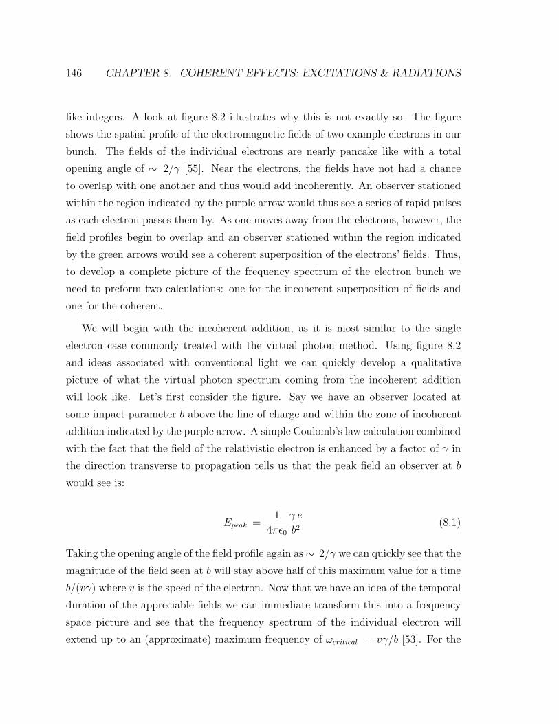
146 CHAPTER 8. COHERENT EFFECTS: EXCITATIONS & RADIATIONS
like integers. A look at figure 8.2 illustrates why this is not exactly so. The figure
shows the spatial profile of the electromagnetic fields of two example electrons in our
bunch. The fields of the individual electrons are nearly pancake like with a total
opening angle of ∼ 2/γ [55]. Near the electrons, the fields have not had a chance
to overlap with one another and thus would add incoherently. An observer stationed
within the region indicated by the purple arrow would thus see a series of rapid pulses
as each electron passes them by. As one moves away from the electrons, however, the
field profiles begin to overlap and an observer stationed within the region indicated
by the green arrows would see a coherent superposition of the electrons’ fields. Thus,
to develop a complete picture of the frequency spectrum of the electron bunch we
need to preform two calculations: one for the incoherent superposition of fields and
one for the coherent.
We will begin with the incoherent addition, as it is most similar to the single
electron case commonly treated with the virtual photon method. Using figure 8.2
and ideas associated with conventional light we can quickly develop a qualitative
picture of what the virtual photon spectrum coming from the incoherent addition
will look like. Let’s first consider the figure. Say we have an observer located at
some impact parameter b above the line of charge and within the zone of incoherent
addition indicated by the purple arrow. A simple Coulomb’s law calculation combined
with the fact that the field of the relativistic electron is enhanced by a factor of γ in
the direction transverse to propagation tells us that the peak field an observer at b
would see is:
Epeak =1
4πε0
γ e
b2(8.1)
Taking the opening angle of the field profile again as ∼ 2/γ we can quickly see that the
magnitude of the field seen at b will stay above half of this maximum value for a time
b/(vγ) where v is the speed of the electron. Now that we have an idea of the temporal
duration of the appreciable fields we can immediate transform this into a frequency
space picture and see that the frequency spectrum of the individual electron will
extend up to an (approximate) maximum frequency of ωcritical = vγ/b [53]. For the

8.2. INCOHERENT VIRTUAL PHOTON SPECTRUM 147
IncoherentSuperposition
CoherentSuperposition
CoherentSuperposition
Figure 8.2: The figure shows two sample electrons from our Gaussian bunch and theirassociated, nearly transverse, field profiles. A look at the field profiles reveals whyone cannot simply add the virtual photon fields of the individual electrons to arriveat the virtual photon field of the entire bunch. In the vicinity of the electrons, thefields do not interfere with one another and would add incoherently. As one movesaway from the electrons, however, the field profiles spatially overlap and thus need tobe added coherently.
the energies used in this experiment and for reasonable impact parameters (discussed
quantitatively below) this incoherent spectrum extends into the hard x-ray regime.
We can now consider the ideas associated with adding photons of conventional
light and extend them to apply to the virtual photons coming from our charge. Con-
ventional incoherent addition of fields leads to a total field proportional the square
root of the number of photons contributing, so here we have a total field proportional
to the square root of the number of charges contributing√
NE. We correspondingly
have an intensity proportional to NE2. Thus, before doing any actual calculation we

148 CHAPTER 8. COHERENT EFFECTS: EXCITATIONS & RADIATIONS
can ascertain that the incoherent contribution to the virtual photon spectrum will
extend into the hard x-ray regime and have an intensity proportional to the number
of electrons in our bunch.
To obtain the virtual photon spectrum we need to take the Fourier transform
of the transverse component of a single electron field, given by equation 4.11. The
result of the transform is given in [32] and here we simply state it, having done the
appropriate SI unit conversions and taken v = c:
E⊥(b, ω) =e
(2π)3/2ε0 b c
bω
cγK1
(bω
cγ
)(8.2)
Here, K1 is a modified Bessel function of the second kind. As discussed in the first
portion of the chapter, the essence of the virtual photon method is to replace the
energy stored in the real electromagnetic field with that stored in a field of equivalent
photons each of energy hω. We first write down the total energy stored in the real
field:
U =
∫
V
ε0 E2⊥(r) dV =
∫
A
∫ +∞
−∞c ε0 E2
⊥(r, t)dt dA =
∫
A
∫ +∞
0
2 cε0 E2⊥(r, ω)dω dA
(8.3)
The integral over A represents the area over which the fields extend (we will see later
that this is roughly over the beam spot). The factor of c is introduced to account for
the change in variable from a spatial to a time coordinate.
Now we need an expression for the energy stored in virtual photons of frequency
ω per unit area per unit frequency so we can equate it to the energy stored in the real
electromagnetic field given by equation 8.3. Taking Nph(ω) as the number of photons
at frequency ω we can write down:
d2U
dAdω= 2 cε0 E2
⊥(r, ω) = hωd2Nph(ω)
dAdω(8.4)
We can divide by h to rewrite the expression on the right in terms of a bandwidth:
d2Nph(ω)
dAdhωhω
=2 cε0 E2
⊥(r, ω)
h(8.5)

8.2. INCOHERENT VIRTUAL PHOTON SPECTRUM 149
Now we simply need to make the substitution with the Fourier transform of the field
to obtain the virtual photon spectrum of a single electron. At this point we can also
replace r with b:
d2Nph(ω)
dA dhωhω
=2 cε0
h
(e
(2π)3/2ε0 b c
bω
cγK1
(bω
cγ
))2
(8.6)
The above expression can be slightly simplified by using the fine structure constant,
αf = e2/(h c 4πε0):
d2Nph(ω)
dA dhωhω
=αfω
2
c2π2γ2K2
1
(bω
cγ
)(8.7)
Equation 8.7 tells us that, due to the properties of the Bessel function, the spec-
trum falls off as ω grows larger than cγ/b, as we already qualitatively ascertained
with our simple argument above. Equation 8.7 also tells us that for any given fre-
quency the number of virtual photons of that frequency decreases with increasing b.
This makes sense in the context of figure 8.2 if we consider only one electron because,
as b increases, the observation cone widens and the observer is thereby exposed to
a temporally longer (and so equivalently lower frequency) pulse. Correspondingly,
there will be fewer high energy photons contributing to the overall spectral density
at that point.
To obtain the total virtual photon spectrum we need to integrate equation 8.7 over
our desired range of impact parameters. Obviously the upper limit of this integration
can go to infinity as there is nothing physically limiting the extent of the photon field.
We can also see that this will immediately be quantitatively checked as the Bessel
function goes to zero at infinity and so automatically limits our spectrum. The lower
limit of integration, or the minimum impact parameter, is not as easy to determine,
however. The minimum impact parameter will determine the maximum observable
frequency (and correspondingly energy) in the virtual photon spectrum according to
the ωmax ∼ cγ/bmin relationship where we have again taken v ∼ c. In practice,
bmin differs depending on the physical process which the virtual photon field will be
used to help describe. For bremsstrahlung, bmin is related to the maximum possible
momentum transfer in the process and is given by h/(2me v) [32]. For collisional

150 CHAPTER 8. COHERENT EFFECTS: EXCITATIONS & RADIATIONS
ionization of atoms it is given by the atomic radius [32]. Since these are the two
processes we are most interested in here we will limit our discussion to them, but
reference [32] has a chart including several of the physical processes discussed in the
chapter seven and their associated appropriate minimum impact parameters.
For the moment we will keep the expression in terms of a generic bmin to finally
arrive at the expression for the total incoherent virtual photon spectrum of a single
relativistic electron:
∫ ∞
bmin
d2 Nph(ω)
dA dhωhω
2π b db =2αfω
2
c2γ2π
∫ ∞
bmin
bK21
(bω
cγ
)db (8.8)
The integral in equation 8.8 does have a closed form solution [56]:
∫xK2
1(ax) dx =1
2x2
(K2
1(ax) − K0(ax) K2(ax))
(8.9)
where for us a would be equal to ω/(cγ). This leaves us the problem of the limits
of integration. Since the modified Bessel functions of the second kind go to zero at
infinity we can take the upper limit as also going to zero. The lower limit will have
a value which we can obtain by substituting bmin. Preforming this substitution and
inserting the appropriate negative sign finally yields our expression for the number of
incoherent virtual photons per unit bandwidth:
dNph(ω)
dhω/hω= − αfω
2
π c2γ2b2min
(K2
1
(bminω
cγ
)− K0
(bminω
cγ
)K2
(bminω
cγ
))(8.10)
To obtain the total spectrum from all of the electrons in our bunch we simply need
to multiply this expression by N .
dNph(ω)
dhω/hω incoherent
= −Nαfω2
π c2γ2b2min
(K2
1
(bminω
cγ
)− K0
(bminω
cγ
)K2
(bminω
cγ
))
(8.11)

8.2. INCOHERENT VIRTUAL PHOTON SPECTRUM 151
8.2.2 Incoherent Spectrum Discussion
Now that we have a calculation for the incoherent spectrum, we want to highlight
some of its characteristics. We will do this for both appropriate minimum impact
parameters, h/(2me v) for bremsstrahlung and a0 (the Bohr radius) for collisional
ionization. Figure 8.3 shows the virtual photon spectra for both bremsstrahlung pro-
duction and collisional ionization, calculated with equation 8.11. For bremsstrahlung
we have used bmin = h/(2me v) = h/(2me c) which is numerically equal to 2·10−13 m.
For collisional ionization we have used a0 = 0.53 A.
We can see from figure 8.3 that the incoherent spectrum extends well into the
hard x-ray and even the gamma ray regime. What this tells us is that there is a
chance for high energy interactions between the individual electrons in the beam
and the sample. This high energy attribute of the spectrum is not surprising, as we
already had the qualitative picture of the spectrum at the beginning of this section
when we stated that the maximum frequency of one electron would be approximately
equal to cγ/b. What the analysis following this simple conclusion gave us is the
information regarding the total number of photons available over a range of these high
energy frequencies. Figure 8.3 shows us that we actually have billions of these high
energy photons accessible to potentially participate in high energy bremsstrahlung
production, collisional ionization, or a myriad of other high energy interactions.
What this begs then, is the question of whether or not this enormous potential
for interaction is actually important for our experiment. The method of virtual pho-
tons, as we have used up to this point, only provides a description of the photons
available for interaction, as we have not actually described any interactions. To carry
the method forward and use it in an actual high energy process we need the cross
sections for photon interaction at each of these energies and, of course, a description
of the sample. Actually preforming these calculations would, however, be fruitless
as we already have the results from the work presented in the last chapter. Before
undertaking the analysis in the this chapter we already knew that bremsstrahlung
production would be a dominant consideration in the energy range of one 28.8GeV
electron, and we already knew that, given our sample composition and thickness, this
production would in practicality be negligible. Carrying out the calculations with the

152 CHAPTER 8. COHERENT EFFECTS: EXCITATIONS & RADIATIONS
100
102
104
106
108
1010
1012
100
102
104
106
108
1010
Photon Energy (eV)
Inco
here
nt V
irtua
l Pho
tons
/ B
andw
idth
Incoherent Virtual Photons per Bandwidth vs. Energy
Bremsstrahlung spectrum, bmin
= 2*10−13 m
Collisional ionization spectrum, bmin
= 0.53*10−10m
Beam Parameters:
N = 1.6*1010 electronsEnergy = 28.8 GeVGamma = 5.6*104
Figure 8.3: The incoherent virtual photon spectra for both bremsstrahlung produc-tion and collisional ionization are shown. The high energy tails of the spectra differbecause of the different minimum impact parameters important for each process.In bremsstrahlung production the interaction can potentially take place at a muchcloser distance than it could for collisional ionization. Numerically bremsstrahlungproduction can occur on distance scales well below the angstrom level while the ion-ization process typically occurs at distances of the order of the atomic radius. Thecloser proximity between the colliding partners in bremsstrahlung leads to the higherfrequency spectrum.

8.2. INCOHERENT VIRTUAL PHOTON SPECTRUM 153
virtual photon spectrum would simply yield identical results.
This is not, however, to say that the virtual photon calculation is without impor-
tance. As was also pointed out in the last chapter, the effects we have considered
thus far only apply to single electrons interacting with the sample. What we have
accomplished is determining that these single electrons can not interact with the sam-
ple to appreciably affect it. This simply means that the information provided by the
incoherent portion of the spectrum is not useful given our larger question of why the
fast pulse leaves the sample damage free and the slow pulse heats it. The inability of
the incoherent portion of the spectrum to help us answer the damage problem is also
underscored by the fact that neither the total pulse length nor the aggregate electric
field value were required as an input to any of the above calculations. It is the in-
formation provided by the coherent virtual photon spectrum, which does incorporate
these factors, which will help us answer the damage question.
Before we leave the topic of the incoherent superposition we want to consider one
final point which illustrates the spatial extent of the effects of the incoherent virtual
photon fields. Figure 8.4 shows the number of virtual photons generated by one
electron vs distance for both bremsstrahlung production and collisional ionization.
The plot shows only the photons at the cutoff frequency (energy) for the particular
process, 5.5·1010 eV for bremsstrahlung and 2.1·108 eV for collisional ionization. The
x-axis is scaled in the units of bmin so we can immediately see that these fields are
extremely short range. Thus, in practice, the hard x-rays do not extend appreciably
outside the spatial extent of the electron bunch, as expected.
At this point we have exhausted the discussion of individual electron effects. It is
clear that the hard x-rays being carried along with our electron bunch could poten-
tially generate significant amounts radiation or free electrons, but, given the results of
the previous chapter, we know this is not the case. Thus, we are ready for a discussion
about the true collective effects of the electron bunch.

154 CHAPTER 8. COHERENT EFFECTS: EXCITATIONS & RADIATIONS
1 1.5 2 2.5 3 3.5 4 4.5 50
1
2
3
4
5
6
7
8x 10
−4
Distance (in units of bmin
)
Inco
here
nt V
irtua
l Pho
tons
Fro
m O
ne E
lect
ron
at
ωc
Incoherent Virtual Photons Produced by One Electron vs. Distance
Bremsstrahlung photons, bmin
= 2*10−13m
Collisional ionization photons, bmin
= 0.53*10−10m
Electron Parameters:Energy = 28.8 GeVGamma = 5.6*104
Each plot is generated with the bmin
and associated cut off frequency ω
c = (γ c)/b
min appropriate for
the physical process.
Figure 8.4: The number of incoherent virtual photons of frequency ωc vs. distance isshown for both bremsstrahlung production and collisional ionization. The distanceaxis is scaled in units of minimum impact parameter, which is different for eachprocess. The number of virtual photons falls off rapidly in each case, and so in bothsituations the field is of extremely short range. In practice, the high frequency fieldsdo not extend appreciably beyond the spatial extent of the bunch itself.

8.3. COHERENT VIRTUAL PHOTON SPECTRUM 155
8.3 Coherent Virtual Photon Spectrum
8.3.1 Coherent Spectrum Calculation
Composing the coherent portion of the virtual photon spectrum is actually quite easy
if one has already has the incoherent spectrum. For the incoherent calculation we
had to go from an expression for the field of an individual electron as a function of
space and time and transform it to a function of space and frequency. We then knew
the frequencies from any individual electron would add to the frequencies of others
only incoherently, so the calculation was essentially complete.
We begin the coherent spectrum calculation with a look back at figure 8.3 which
shows us that the frequency spectrum for each individual electron does extend down
to much lower energies and wavelengths than the hard x-ray regime. We know that
it is these lower energy, longer wavelengths which can potentially add up coherently
over a long range. A look back at figure 8.4 reminds us that this is impossible for
the shorter wavelength, shorter range hard x-ray photons. We thus now just have to
figure out how to appropriately undertake this coherent addition.
Before doing any math, we can use a pictorial argument to ascertain what wave-
lengths will make up the coherent virtual photon spectrum. Figure 8.5 shows electron
bunches of two temporal lengths and so approaches the problem from a slightly dif-
ferent perspective. On the left side of the figure is an electron bunch where the bunch
length is much greater than the emitted wavelength. In this case the emitted radi-
ation is out of phase and consequently adds incoherently. On the right is a bunch
where the emitted radiation’s wavelength is of the order of the bunch length. This
enables the radiation to be coherent, as the electron fields add in phase. The idea
we need here is the same: wavelengths comparable to and longer than the bunch
length will add up coherently and wavelengths shorter than the bunch length will
add up incoherently. We can now again use the idea of a pulse width defining a
characteristic frequency to see that a pulse 70 fs in duration will correspond to a co-
herent frequency spectrum extending into the terahertz, specifically 2.3THz, where
1THz =1012 Hz. 1THz corresponds to the far infrared wavelength of 300 µm and a
photon energy of 4.14meV. We will discuss the attributes of terahertz at length at

156 CHAPTER 8. COHERENT EFFECTS: EXCITATIONS & RADIATIONS
Bunch lengththan
wavelength
longer
incoherent fields®
Bunch lengththan
wavelength
shorter
coherent fields®
Figure 8.5: The length of an electron bunch in space relative to the wavelength of itselectrons determines if the bunch will radiate coherently. On the left side of the figurethe electron’s wavelength is smaller than the extent of the bunch and the electronsfields hence add out of phase. On the right side of the figure the wavelength iscomparable to the bunch length and the electrons can add up coherently.
the end of the chapter, as its features play an important role in the elucidating the
(lack of) heating effects observed with the compressed bunch. At this point it is also
valuable to mention the uniqueness of the SLAC compressed electron bunches. Before
the introduction of the special chicane discussed in chapter four the electron bunches
could not be compressed into the femtosecond regime, and consequently it was im-
possible for them to produce coherent radiation in the THz band. It is thanks to the
relatively new advancements in accelerator physics that such a coherent addition is
possible [30]. Our longer, 2.3 ps electron bunch will have a coherent spectrum which
lies at longer (microwave) wavelengths and this will also be discussed.
For a final, qualitative, point we can again appeal to the addition of light waves
and ascertain that for coherent fields the total field will be proportional to NE and
the intensity to (NE)2.
Taking the above discussion into account, we see that we can actually begin the co-
herent virtual photon calculation with the end of the incoherent one: we already have
the Fourier transforms of the individual electron fields, we now just need to mathe-
matically ascertain which of those frequency components will superimpose coherently.

8.3. COHERENT VIRTUAL PHOTON SPECTRUM 157
The coherent enhancement due to electron bunching was first predicted in [57] and
the theoretical derivation of coherent radiation emitted from bunched electron beams
was carried out in [58]. A nice summary and slightly more transparent formulation
of the problem are also given in [59]. Here we will simply go through the qualitative
logic and state the mathematical results pertinent for our Gaussian bunch.
The superposition calculation can be done for a discrete distribution of electrons,
but in practice the positions of the 1010 electrons within our small bunch volume are
indistinguishable in the rest frame of the laboratory so we are justified in taking the
electron distribution as a smooth Gaussian in each direction. We can then define a
position vector from any point in the distribution to an observer who, for the moment,
we will leave with a generic position. The observer will have some distance from the
center of the distribution and also an associated angle of observation. We will take the
angle of observation as θ and assign on-axis observation as θ = 0. This means that if
the observer is along the z axis in our geometry θ = 0. We are going to construct our
coherent spectrum in analogy with our incoherent one which here means θ = 0. At
first it might seem like we should choose π/2 given our earlier discussion and figure
8.1 but this is not so because of how we are going to add up the fields: The total
number of photons from the bunch measured at the point of the observer will be
the integral over all of the electric field contributions from the charge distribution,
each with an appropriate phase factor. It is the phase factor which will give us our
coherence at any certain frequency. This means that if we have an on-axis observer
the integral will sweep out a symmetric Gaussian ellipsoid like shape over the bunch
volume, and correspondingly collect all of the phase information symmetrically. Off
axis observation would destroy this symmetry. We will see mathematically below that
this symmetry in the geometry also allows the transverse distribution of electrons to
drop out of the calculation.
Preforming this integral over space actually gives you two terms. The first repre-
sents the spectrum of a single electron multiplied by the number of electrons in the
bunch. Hence, it the incoherent spectrum which we already already obtained through
different means and showed in equation 8.11. The second term is the coherent term,
and it is represented as a function of the incoherent spectrum:

158 CHAPTER 8. COHERENT EFFECTS: EXCITATIONS & RADIATIONS
d2Nph(ω)
dhω/hω coherent
=d2Nph(ω)
dhω/hω incoherent
N f(ω, θ) (8.12)
Here f(ω, θ) is the bunch “form factor.” It is the Fourier transform of the three di-
mensional bunch distribution in real space, and so takes into account the longitudinal
electron distribution which dictates our level of coherent superposition. The form
factor also takes the transverse distribution into account to accurately capture the
interference effects over the continuous bunch distribution. For a Gaussian bunch the
form factor is:
f(ω, θ) = exp(−(ωσr sin(θ)/c)2
)exp
(−(ωσz cos(θ)/c)2)
(8.13)
Since we are formulating our problem with θ = 0, the sin(θ) term drops out and the
form factor reduces to:
f(ω) = exp(−(ωσz/c)
2)
(8.14)
this is the aforementioned elimination of the transverse distribution in the formulation
of the coherent spectra. We can also immediately see that, since our incoherent
spectrum scaled with N , our coherent spectrum scales with N2 as we already guessed
from the analogy with light.
This finally yields our expression for the coherent virtual photon spectrum of our
bunches:
dNph(ω)
dhω/hω coherent
=dNph(ω)
dhω/hω incoherent
N exp(−(ωσz/c)
2)
(8.15)
8.3.2 Coherent Spectrum Discussion
We can now discuss some features of the coherent virtual photon spectrum. We start
by obtaining the virtual photon spectrum for a verity of different pulse widths by
changing the value of σz in equation 8.15. For the calculation we have used the impact
parameter appropriate for bremsstrahlung production. Before we show the plot, we
do need to address this last point about the impact parameter being important for

8.3. COHERENT VIRTUAL PHOTON SPECTRUM 159
the coherent calculation. It would at first seem that the parameter necessary to
characterize the high energy interactions of the bunch (which have their source in the
incoherent photons) should not be important for the coherent calculation which is
more concerned with the overall distribution of electrons in the bunch as a collective
pulse. The tie becomes necessary because of energy considerations. We of course have
to ensure that the total energy contained in the virtual photon spectra does not exceed
the energy of the original electron bunch (N ·28.8GeV). This former number is the sum
of the coherent and incoherent parts. A smaller impact parameter for the high energy
processes allocates more energy to the incoherent spectrum and so, in accordance with
equation 8.15 also allocates more energy to the coherent spectrum. The total energy
contained in each portion of the spectrum will be addressed later in the chapter, but
for each case, whether we take bmin for bremsstrahlung or collisional ionization, we
have total energies contained in the virtual photon spectra which are smaller than
the total energy of the bunch. Physically, this reflects the fact that there are simply
no processes (which we are considering here) which can liberate the extremely high
energy photons carried along with the electron bunch. It is actually this energy
transfer cutoff which sets the impact parameter, as discussed in the beginning of the
chapter. This most definitely does not, however, mean that we can take the impact
parameter down to zero to recover the total energy in the bunch. Mathematically,
this is because the Bessel functions in all of our expressions diverge at the origin.
Physically, this tells us that it is the energy of the individual electrons which actually
sets the upper frequency limit of the available photons. Taking any impact parameter
which gives energies higher than this is not physical and will yield incorrect results.
While this seems like it could be a point of complication, we will see later that the
coherent excitations and radiations we consider in relation to the coherent spectrum
do not liberate as much real energy as we have the potential to liberate from the
virtual spectrum, even with the collisional ionization bmin, so the problem becomes
largely moot and will not be considered any further.
The coherent spectrum is shown in figure 8.6 and there are a few important points
we should highlight. First, we see that the number of high energy photons decreases
as the pulse width increases, which is not surprising. Second, we see that the number

160 CHAPTER 8. COHERENT EFFECTS: EXCITATIONS & RADIATIONS
10−4
10−3
10−2
10−1
104
106
108
1010
1012
1014
1016
1018
1020
Photon Energy (eV)
Coh
eren
t Virt
ual P
hoto
ns /
Ban
dwid
th
Coherent Virtual Photons vs. Energy
τ = 70 fsτ = 500 fsτ = 2.3 ps
Pulse Length:
Beam Parameters:N = 1.6*1010
Energy = 28.8 GeVGamma = 5.6*104
Figure 8.6: The coherent virtual photon spectrum is shown for three different bunchlengths. The number of high energy photons is reduced as the pulse width gets longerin time, which is not surprising. The most important feature of the plot is the energyrange over which the photons span. For the short, τ = 70 fs pulse, the spectrumextends well into the terahertz.
8.4. TOTAL VIRTUAL PHOTON SPECTRUM 161
of coherent virtual photons per bandwidth is approximately 10 orders of magnitude
higher than the number for the incoherent spectrum, which reflects the coherent
spectrum’s N2 dependence. Again this is not surprising. The most important feature
of the plot is the energy range over which the photons span. For the short, τ = 70 fs
pulse, the spectrum extends into the terahertz. This is actually quite remarkable as
intense sources of terahertz radiation are quite rare, and this topic will be treated
later in the chapter. It should also be noted that the plot contains the number of
coherent photons included in both our τ = 70 fs electron bunch and our τ = 2.3 ps
electron bunch.
To continue to mirror the discussion of the incoherent spectrum, we now consider
the spatial extent of the coherent spectrum. We cannot do this in exact analogy
with the incoherent photons, however, as with the incoherent photons we were free
to only look at how the field decreased from one electron. Here, we need to take the
coherence effects into account. To do this, we use equation 8.15 and integrate it over
all frequencies for several, increasingly large minimum impact parameters. What this
actually gives us is the number of virtual photons of all frequencies which would be
produced taking that impact parameter as bmin. Physically, this means we obtain
the number of virtual photons that would be present outside that bmin. Thus, what
is actually plotted is the number of photons present outside each radial distance. In
this way the overall information about the distance dependence of the spectrum is
maintained. It is actually quite convenient that we do not have to worry about setting
the limits of integration exactly right, as the form factor will handle the appropriate
coherence effects for us. The plot is shown in figure 8.7
Now that we have both the incoherent and coherent virtual photon spectrums
and their spatial characteristics we are equipped to discuss the total virtual photon
spectrum of the beam.
8.4 Total Virtual Photon Spectrum
We can now piece together the incoherent and coherent virtual photon spectra to
look at the total spectrum of photons carried by the electron bunch. To obtain the

162 CHAPTER 8. COHERENT EFFECTS: EXCITATIONS & RADIATIONS
0 1 2 3 4 5 6 7 8 9 101.6
1.7
1.8
1.9
2
2.1
2.2
2.3
2.4
2.5x 10
22
Distance (R) (millimeters)
Nu
mb
er o
f C
oh
eren
t P
ho
ton
s o
f A
ll F
req
uen
cies
Ou
tsid
e R
Spatial Profile of the Coherent Virtual Photon Spectrum
Beam Parameters:
N = 1.6*1010
σz = 21 µm (τ = 70 fs)
Figure 8.7: The spatial profile of the coherent virtual photon spectrum is shown.What is plotted is not the number of photons vs. distance, but rather the numberof photons present outside each distance, as explained in the text. The fact that wehave included all frequencies means that we are seeing the THz photons and photonsof lower energies as well. The plot simply shows everything which is coherent. The xaxis is in millimeters, showing that these photons are of quite long range.

8.4. TOTAL VIRTUAL PHOTON SPECTRUM 163
total spectrum we simply need to sum the incoherent and coherent parts, with one
small modification. We have used the incoherent spectrum to obtain the coherent
one, which means that if we simply added them we would double count those low
energy photons. We thus simply need to remove them. This makes the expression
for the total virtual photon spectrum:
dNph(ω)
dhω/hω full
=dNph(ω)
dhω/hω incoherent
(1 + (N − 1)exp
(−(ωσz/c)2))
(8.16)
The total spectrum for the compressed τ = 70 fs electron bunch is shown in figure
8.8 for two cases. The spectrum shown by the dashed blue line is calculated with a bmin
appropriate for bremsstrahlung production and the solid pink line is calculated with
a bmin appropriate for collisional ionization. The coherent portion of the spectrum is
also calculated using the appropriate impact parameters.
The most important feature of figure 8.8 is that the number of coherent photons
dwarfs the number of incoherent photons by approximately 10 orders of magnitude.
This is not surprising as we already knew that the number of coherent photons would
scale with N2 while the incoherent would scale only as N before we started the exact
calculation of the spectra. Because we have of the order of 1010 electrons in our
bunch we would expect such a difference. The other difference in the spectra which
should be reemphasized at this point is that the incoherent spectrum depends on the
impact parameter and on the energy of the individual electrons in the bunch while the
coherent spectrum depends on both of these and the longitudinal bunch distribution.
Before we move on it is useful to point out one of the practical differences be-
tween the frequency spectra which we just derived and that of a conventional half-
cycle pulse. The electric field frequency spectrum of the unipolar half-cycle pulse
produced by the charged particle bunch has a DC component. This is evident be-
cause the Fourier transform of the entire Gaussian bunch has a DC component. This
correspondingly means the magnetic field also has a zero frequency component and
this fact is of key importance as we use this component to initiate our magnetic field
switching. If we had the type of half-cycle pulse created by true electromagnetic waves

164 CHAPTER 8. COHERENT EFFECTS: EXCITATIONS & RADIATIONS
10−4
10−2
100
102
104
106
108
1010
1012
1012
106
108
1010
1012
1014
1016
1018
1020
Photon Energy (eV)
Tot
al V
irtua
l Pho
tons
/ B
andw
idth
Total Number of Virtual Photons vs. Photon Energy
Incoherent bmin
for bremsstrahlung production
Incoherent bmin
for collisional ionization
Beam Parameters:
Ne = 1.6*1010
Energy = 28.8 GeVGamma = 5.6*104
τ = 70*10−15 sec
The plot shows the total number of virtual photonsas a function of photon energy. The dashed blue curve represents the total spectrum when the incoherent portion is calculated with a b
min appropraite for
bremsstrahlung production and the solid pink curve the total spectrum with a b
min appropraite for collisional ionization.
Figure 8.8: The total virtual photon spectrum for a τ = 70 fs electron bunch is shown.Two cases are calculated, the spectrum shown by the dashed blue line represents abmin appropriate for bremsstrahlung production and the solid pink line represents abmin appropriate for collisional ionization. The coherent portion of the spectrum isalso calculated with the appropriate impact parameters. The most important featureof the spectrum is that the total number of coherent terahertz photons is higher thanthe total number of high energy incoherent x-ray photons by roughly 10 orders ofmagnitude.

8.5. TERAHERTZ SCIENCE - A BRIEF INTRODUCTION 165
(ie no DC component and a long, low-amplitude negative tail) this would mean we
would eventually have a magnetic field of opposite polarity to that which we started
with and the total time integral of the magnetic field would be zero. This could mean
that the sample would “switch back” during the negative tail of the pulse. There is a
possibility (probability) that this second reversal would not be observable, however,
because as just noted this tail is usually very long and of very low amplitude (see
especially reference 36 in [27]). If there is not enough energy present in the sample at
one point in time to overcome the inherent anisotropy barriers the sample could not
switch again, even though the overall integral of the field is still zero. Additionally,
this entire consideration could be dwarfed if the E field is strong enough to initiate
switching, as that effect goes as E2 as described at the end of chapter six.
Before concluding our discussion, we include one final plot which shows the total
virtual photon spectra for both the τ =70 fs and τ =2.3 ps electron bunches. We can
see that the incoherent, high energy portions of the spectra overlap as expected. For
the lower energy, coherent spectra we can see that the 70 fs pulse has photons of a
higher, THz energy contributing to its spectrum while the 2.3 ps bunch has a lower
frequency cutoff. Figure 8.9 shows the plot.
This completes our discussion of the virtual photon description of the beam and
enables us to move onto a discussion of how the THz photons produced by the col-
lective effects of the bunch can affect our sample. One more look at figure 8.7 tells
us that the spatial extent of these photons will reach beyond well beyond 500 µm.
This means the THz photons can potentially drastically change the character of our
sample on distances scales clearly observable over the scope of our switching pattern.
8.5 Terahertz Science - A Brief Introduction
Before we can have a discussion about how the THz photons produced by the collective
effects of the beam affect our sample we need to have a short discussion about the
features of THz radiation in general. THz radiation falls in between the infrared
and microwave frequency bands and, while the exact width of the band varies in the
literature, it is generally accepted to fall between ∼ 100GHz and ∼ 10-30THz [60,61].

166 CHAPTER 8. COHERENT EFFECTS: EXCITATIONS & RADIATIONS
10−5
100
105
1010
106
108
1010
1012
1014
1016
1018
1020
Photon Energy (eV)
Virt
ual P
hoto
ns /
Ban
dwid
th
Virtual Photons vs. Energy for Short and Long Bunches
τ = 2.3 psτ = 70 fs
Pulse Length
Beam Parameters:
N = 1.6*1010
Energy = 28.8 GeVGamma = 5.6*104
Figure 8.9: The total virtual photon spectrum for the τ = 70 fs and τ =2.3 ps elec-tron bunches are shown. Both have been calculated with the bmin appropriate forbremsstrahlung production. The most important features are that the high energy,incoherent spectra overlap while the lower energy, coherent spectra differ. The sourceof the difference is the variable longitudinal distribution of the respective electronbunches, as discussed in the text.
Figure 8.10 shows the THz portion of the spectrum and specifically highlights its
placement between the more historically comfortable regions of electronics (beneath)

8.5. TERAHERTZ SCIENCE - A BRIEF INTRODUCTION 167
and photonics (above). Until recently the frequency band has been characterized
as the “Terahertz Gap” due to its inability to be accessed with either conventional
microwave electronics or typical photonic techniques. This name is currently fading
as numerous approaches are now making the frequencies more accessible [62].
Figure 8.10: The figure shows the entire electromagnetic spectrum and highlightsthe terahertz region, lying between ∼ 100GHz and ∼ 10-30THz. Historically thefrequency bands on each side of the THz window have been readily harnessed inboth academic and industrial applications. The THz region, however, representsfrequencies too short to be accessed with conventional microwave electronics andtoo long to be within the grasp of typical photonic techniques. Until recently, thefrequency band has been thus characterized as the “Terahertz Gap” but this name isfading as numerous techniques are now making the frequencies more accessible [62].Figure reprinted by permission from Macmillan Publishers Ltd: Nature Materials [60],copyright 2002, http://www.nature.com/nmat/index.html
Historically, the primary utilization of THz radiation has been in spectroscopic
studies undertaken by chemists and astronomers. This work focused on THz emit-
ters, as it was mainly concerned with characterizing rotational and vibrational reso-
nances and thermal-emission lines of simple molecules. Empirically these studies were
not well funded due to the difficulty of dealing with high atmospheric absorption of
the emission lines. Over the course of the past two decades, however, the field has
taken a new direction and a good deal of research has been dedicated to building
and using THz sources. These new sources and applications span the fields of pure

168 CHAPTER 8. COHERENT EFFECTS: EXCITATIONS & RADIATIONS
research, semiconductor devices, medical applications, quality control in manufactur-
ing, homeland security, space science, defense, and many more [60]. Some of the most
exciting scientific applications include studying small molecule rotations, collisions of
molecules in the gas phase, collective vibrational modes of proteins, intermolecular
vibrations in molecular crystals, intra-exciton and intra-impurity transitions in semi-
conductors, and various excitations in superconductors [62,63]. Additionally, the po-
tential for THz spectroscopy is rapidly expanding as Fourier transform spectroscopy,
narrowband spectroscopy, and THz time-domain spectroscopy techniques are all in-
creasing in sophistication [60, 61]. The information and communication technology
sectors are also beginning to see the benefits of THz through wireless communication,
high-speed data processing, and satellite communications [61].
From both pure scientific and application standpoints, there are two main prop-
erties of THz which make it appealing. First, it is non-ionizing due to its relatively
low energy (recall that 1THz corresponds to 4.14meV). This makes it particularly
well suited for biological imaging and testing applications as it will not damage liv-
ing tissue [64], and particularly well suited for some classes of materials studies as it
does not have enough energy to excite common interband transitions. Second, while
THz wavelengths readily penetrate common materials such as clothing and packaging,
there are several absorption lines in the band which correspond to biological materi-
als of interest, such as water and common tissues, and several absorption lines which
correspond to common illegal drugs and plastic explosive material. This combination
of features is why practical THz technology is of keen interest to both the medical
community and the department of homeland security [65].
The reason we do not see tremendous numbers of THz applications at work is
simply because the existence of high powered and either broadband or tuneable nar-
rowband sources of THz radiation have empirically been extremely limited, hence
the previous “Terahertz Gap” comment. Currently there are a few sources commer-
cially available, but most of the progress in THz production has come from academic
laboratories.
A common way to classify the available THz sources is by the type of radiation
they produce. There are three. First, there are incoherent thermal sources, such as

8.5. TERAHERTZ SCIENCE - A BRIEF INTRODUCTION 169
black body radiators, which produce broadband continuous emission. While these
radiators, such as filament lamps and fluorescent sources, are typically good emitters
of high frequency radiation (ultraviolet, visible, and infrared) it is difficult to obtain
significant power levels of THz from them. A typical output is of the order of 1 nW
per wave number [66]. A recent experiment using a heated rod of silicon carbide as
the emitter did, however, achieve a total power of 120 µW below 1THz [67].
Second, there are broadband pulsed sources. Most of these are based on the exci-
tation of a material with an ultrashort laser pulse. Some of the most popular methods
use lasers to accelerate photocarriers in photoconducting antennas, generate second-
order non-linear effects in electro-optic crystals (as in optical rectification), or generate
plasma oscillations. These sources are also troubled by low output powers. Typical
conversion efficiencies of the techniques yield THz beam powers in only the nW to µW
range when starting with optical sources of about 1W. In general the output powers
of the photoconductive emitters have slightly higher powers and smaller bandwidths
(up to 40µW and 4THz) than optical rectification techniques (bandwidths of 50 THz
with tunable center wavelengths) [60] (and references therein).
Thirdly, there are narrowband continuous wave sources. These sources can rely on
either upconversion of typical radio frequency sources or downconversion of optical
sources. The upconversion techniques will typically yield powers less than 100 µW
[60]. Gas lasers provide another narrowband source when they act as a pump of a low-
pressure gas cavity which then lases at the gas molecules’ emission-line frequencies.
These sources are not smoothly tunable, but they can provide output powers up
to 30 mW. Non-linear photomixing is another technique where two continuous wave
laser sources with slightly different center frequencies are mixed in a material with
strong second-order optical non-linearities to produce THz via interference. Finally,
parametric generators and oscillators can be utilized. These and a verity of other
continuous wave optical techniques can generate output powers in excess of 100mW if
they are run in a pulsed mode [60]. Perhaps the best known narrowband THz sources
are semiconductor lasers, particularly the quantum cascade laser. The cascade lasers
have continuous wave output powers up to tens of milliwatts [61], but they historically
have operated only at low temperatures, below ∼ 178K [68]. A recent experiment has

170 CHAPTER 8. COHERENT EFFECTS: EXCITATIONS & RADIATIONS
broken this barrier however, and has an operational cascade laser at a temperature
of 225K [69]. The group estimates their output power to be in the 1-2mW range.
There are also several “non-conventional” sources of THz. For instance, solid
state electronic devices now contribute at the extremely low end of the THz fre-
quency window [61] (and references therein). There is also a continually expanding
list of new sources including, for example, resonant tunneling diodes and plasma-wave
photomixers [61]. Other methods of generation currently under investigation include
subjecting crystalline polarizable materials to shock wave excitations which can gener-
ate weak but narrow-band temporally coherent radiation in the 1-100THz range [70]
and using difference-frequency mixing of two parametrically amplified pulse trains
from a single white-light seed to generate tunable pulses with amplitudes exceeding
100MV/cm [71].
There are also two increasingly common generation mechanism which we have al-
ready hinted at: synchrotron radiation from a compressed electron bunch generated
when the bunch passes through a bending magnet [72–74] and transition radiation
created when an electron bunch passes through the interface between media of differ-
ent refractive indices [75–77]. The former has seen peak output powers of up to 106 W
and can also generate either continuous or pulsed waves [60]. For the latter, electrons
accelerated in a typical accelerator such as SLAC or Jefferson Lab’s are not necessary
as laser wakefield accelerators are now producing electrons which can subsequently
generate THz of high peak powers [75]. The output energies of these laser acceler-
ator sources are high, with some reaching into the microjoules of output per pulse.
Another group has developed a technique to produce tunable, coherent, broadband
terahertz radiation by modulating electrons in a storage ring with a femtosecond laser
pulse [78, 79]. These techniques are obviously limited by the magnitude and cost of
the facilities needed to produce them.
The above look at typical THz sources and characteristics is by no means meant
to be a comprehensive review of the field, as that is well beyond the scope of this
thesis. The goal of this section was to simply introduce the field to give a context for
comparison between these sources and the SLAC beam. This comparison is the topic
of the next section.

8.6. TRADITIONAL THZ SOURCES VS. THE SLAC BEAM 171
8.6 Traditional THz Sources vs. the SLAC Beam
As is likely obvious after reading the previous section, most groups who work in THz
generation characterize their source by its output power, and these typically range
from the milliwatts to microwatts for the tabletop sources and upwards of megawatts
for some of the accelerated-electron based sources. The quantities of greater interest
for this thesis, however, are the total THz energy emitted and the magnitude of the
electric field, as we have framed a large portion of our discussion around the energy
contained in the coherent virtual photon field of the SLAC bunch or the strength of
the electric field we need to appreciably distort the valence states of our material. We
will correspondingly move forward in two directions. First we will characterize the
SLAC beam in terms of output THz power, and second we will consider the electric
fields produced by the THz sources discussed in the previous section.
Before we look at the coherent THz output power of the SLAC beam (a broadband
pulsed source) it is useful to look at two other numbers. The first is the total power
carried by the compressed τ = 70 fs bunch and the second is the portion of that
power contained in the total coherent portion of the spectrum. We first find the total
power by using the fact that we have 1.6·1010 electrons in the bunch each at 28.8GeV.
Converting this to Joules and taking the full pulse width as 140 fs we obtain:
Ptotal = 28.8 · 109 · 1.6 · 1010 · 1.602 · 10−19 · 1
140 · 10−15= 5.3 · 1014 Watts (8.17)
To obtain the portion of this power carried by the coherent virtual photons we can
integrate the full coherent spectrum shown in figure 8.6. This yields 2.97·1017 eV and
a corresponding power of:
Pcoherent = 2.97 · 1017 · 1.602 · 10−19 · 1
140 · 10−15= 3.40 · 1011 Watts (8.18)
Finally we can take only the portion of the spectrum shown in 8.6 above ∼100GHz
to obtain the total THz power:

172 CHAPTER 8. COHERENT EFFECTS: EXCITATIONS & RADIATIONS
Pcoherent THz = 9.77 · 1016 · 1.602 · 10−19 · 1
140 · 10−15= 1.12 · 1011 Watts (8.19)
This number is obviously much higher than any of the values quoted in the previous
section. Even though the SLAC compressed electron bunches are a stronger source
of THz than any of the sources treated in the last section, this is still somewhat of
an unfair comparison for two reasons. First, and most trivially, some of the powers
quoted in the previous section are average powers, and we have quoted a peak power
from a pulsed source. Second, and more importantly, at this point our electron beam
is still only a source of virtual THz photons. To be a source of true THz radiation
the virtual photon field has to be liberated from the electron bunch in some fashion,
be it through transition radiation by passing through a foil or synchrotron radiation
by going through a bending magnet etc. The calculation we have performed has only
given us the upper limit on the THz radiation our electron bunch could produce. This
is in contrast to the THz sources discussed in the previous section as they are emitting
true electromagnetic radiation. We will revisit this point later in the chapter.
Consequently this is an ideal point to frame the comparison in the context of
electric fields. We know the compressed SLAC pulse has a peak electric field of
20GV/m just outside the edge of the bunch, and that the number of incoherent x-ray
photons falls off quickly as we move away from the central distribution of electrons.
What this tell us is that, outside the confines of the electron bunch, we can look at the
electric field seen by our sample’s atoms as coherent and lying at least partially in the
THz. In other words, it is fair to say that an appreciable portion of the short pulse
field represented by figure 4.9 outside of the bunch radius is coherent and near the
THz band. This means that all of the sample atoms along one line radially outward
from the point of impact of the bunch (ie, along an electric field line) will experience
the in phase addition of photon fields yielding an extremely strong THz pulse. To
underscore this point, figure 8.11 shows the spatial profile of only the THz virtual
photons generated by the τ = 70 fs electron bunch. By comparing this figure to
figure 8.7 we immediately see that outside the bunch an appreciable portion of the

8.6. TRADITIONAL THZ SOURCES VS. THE SLAC BEAM 173
virtual photon energy is contained within the THz frequency band.
0 1 2 3 4 5 6 7 8 9 102
2.5
3
3.5
4
4.5
5
5.5
6x 10
21
Distance (R) (millimeters)
Nu
mb
er o
f C
oh
eren
t P
ho
ton
s o
f T
Hz
Fre
qu
enci
es O
uts
ide
R
Spatial Profile of the Coherent THz Virtual Photon Spectrum
Beam Parameters:
N = 1.6*1010
σz = 21 µm (τ = 70 fs)
Only frequencies above 100 GHz are used to obtain the plot
Figure 8.11: The figure shows the spatial profile of the THz virtual photons generatedby the τ = 70 fs electron bunch. This figure is generated in the same way as figure8.7, which means that at each point the graph’s value reflects the number of coherentTHz photons present outside that radius. By comparing these numbers to those infigure 8.7 we see that an appreciable portion of the coherent virtual photon energycarried by the bunch is in the THz band.
This leaves us with characterizing the electric fields produced by the THz sources

174 CHAPTER 8. COHERENT EFFECTS: EXCITATIONS & RADIATIONS
summarized in the previous section. In the literature it is common to see plots of the
peak electric field from a THz emitter, but it is commonly scaled in arbitrary units
making a quantitative comparison impossible. The general problem is to define a spot
size over which the power is collected. We will not discuss this point, however, because
reasonable estimates for the spot size quickly tell us that the typically observed THz
fields for most of the tabletop sources discussed early in the previous section are several
orders of magnitude off of what we can obtain with the SLAC electron bunches. For
example, both photoconductive antennas and quantum cascade laser sources have
typical peak fields in the kilovolt per meter range [80, 81]. Optical rectification does
begin to reach into the high field regime as it can obtain the megavolt per meter
limit [82] and under certain circumstances achieve 108 V/m [83]. There is also the
technique which achieved 100MV/cm =10GV/m mentioned in the last section [71]
which does rival our field. For the electron based sources there is also the difficulty
of extracting a true peak electric field value. A Brookhaven group has quoted a value
of the order of 107 V/m [77].
What we can confidently say about our relativistic electron bunches as sources of
coherent THz radiation is that they are on the upper cusp of the accessible energy,
power, and electric fields of any of the sources available today and thus provide us
with a unique opportunity to study their influence on our metallic magnetic system.
8.7 Possible Resolution of the Heating Dilemma
The goal of this section is to propose a possible explanation for the observed discrep-
ancy in the heating effects induced by our varying bunch lengths. As the discussion
progresses, we will see that this heating problem is inextricably linked with the ques-
tion of how the energy of pulse was originally absorbed by the sample. Before we
propose the explanation it is helpful to review what we already know:
1. The analysis of the magnetic data in chapter six confirmed that the strong electric
field of the compressed electron bunch penetrates our metallic sample. This is due
8.7. POSSIBLE RESOLUTION OF THE HEATING DILEMMA 175
to the combination of the field being ultra relativistic (and thereby preventing any
pre-screening) and the film being thinner than its 50 nm skin depth. We can also sur-
mise that the smaller electric field of the uncompressed τ =2.3 ps bunch most likely
penetrates our sample because those electrons have the same relativistic γ factor as
those of the compressed bunch and thus will also not be screened before their arrival
at the sample surface. We do not have the same direct physical evidence of this,
however, as we have with the compressed pulse as the transient magnetoelectronic
anisotropy (ie the conclusive evidence for the presence of the electric field) goes pre-
dominantly as E2 which makes it impossible to observe with the ∼ 33x weaker field
of the uncompressed bunch. What we have observed, however, is the heating of the
sample and this most likely has its source in an electronic excitation of some kind
which thereby necessitates the presence of at least some electric field inside the sample.
2. The Monte Carlo simulations discussed in chapter seven tell us that the direct elec-
tron beam does not deposit enough energy in the sample to produce any detectable
heating or ablation and that it largely passes through the sample unperturbed. These
simulations considered the interaction between one high energy electron and the sam-
ple at a time, meaning they were not time dependent and did not take into account
any collective beam effects. This means that the results are applicable for both the
compressed and uncompressed bunches. The incoherent virtual photon spectrum de-
rived in this chapter agrees with this interpretation, as it tells us the energy spectrum
from the direct beam is incoherent and lies in the x-ray regime. Since x-rays have a
negligible chance of interacting with our thin material it is not surprising that they
largely pass through it without depositing any energy.
3. The compressed femtosecond bunch has a corresponding coherent frequency spec-
trum which extends into the THz due to the bunch length being comparable to THz
wavelengths. This is a collective effect due to all of the electrons and so will not be
the same for the longer, uncompressed bunch. We also know that the uncompressed
picosecond bunch carries with it a coherent portion of its spectrum, but that it will
be of longer, microwave wavelengths as 1/(2 π · 2.3 ps)= 6.9·1010 Hz.

176 CHAPTER 8. COHERENT EFFECTS: EXCITATIONS & RADIATIONS
4. THz (and microwave) wavelengths are too low in energy to excite any interband
transitions in our transition metal film. While we do not have the exact band struc-
ture for our sample, typical transition metals have their lowest interband transition
energies lying upward of 700meV [84]. This means a single half cycle pulse of THz
or microwave radiation will not deposit any energy in the electron gas through this
channel.
The proposed solution to why the picosecond length pulse heats the sample and
why the femtosecond one does not begins with a simple physical principle: when you
apply an electric field to a metal it will generate a current. One typically expects
that this current will increase linearly with the applied field in accordance with Ohm’s
law and that the current flow will lead to a deposition of energy and corresponding
heating of the sample. This is normal Joule heating. The energy density deposited
in a sample from a Gaussian current pulse is given by:
Energy Density =
∫ ∞
−∞σ E2(r, t) dt =
√πσ E2(r)τ (8.20)
where σ is the conductivity of the material and τ is the pulse width. We take σ
as 107 A/(Vm) and do this calculation for our field profile at a distance of 100 µm
from the center of the bunch. For the compressed bunch this yields an energy density
deposited of 9·103 eV/atom and for the uncompressed bunch an energy density of
281 eV/atom. Here we have used a density of 9.04·1022 atoms/cm3 calculated from
the 8.71 g/cm3 density of Co70Fe30. Clearly, we do not observe an energy deposition
anywhere close to these values even with the longer picosecond bunch, as this is
enough energy to completely obliterate the sample. For comparison, the Curie point
of our sample is equivalent to 0.1 eV/atom.
The calculation is inaccurate simply because it relies on the linear relationship
inherent in Ohm’s law, which is not always valid and specifically breaks down in the
high electric field regime [85]. While we consequently cannot take anything quantita-
tive from the calculation we can consider the original principle that when an electric

8.7. POSSIBLE RESOLUTION OF THE HEATING DILEMMA 177
field is applied to a metal a current flows which will ultimately produce heat. We can
also add that this heat is produced in scattering events between the conduction elec-
trons, phonons, impurities, and defects in the conductor. To arrive at the difference
between the observed heating effects with our two pulse widths we thus need to look
how the excitations applied to our conductor in this non-linear regime differ in each
case and how those excitations will affect the mechanisms for heat generation.
8.7.1 High-Field Excitations in a Band Model
We can begin with a simple model where we look at one dimensional conduction in a
row of atoms equally spaced and oriented along a line parallel to the applied electric
field, E. This gives us a simple periodic potential and a band structure like that
shown in figure 8.12. The figure shows the first Brillouin zone of the one dimensional
lattice with lattice spacing a. The band is shown as half filled, as would be typical
for a metal.
k
E
p
ap
a
Figure 8.12: The first Brillouin zone of a simple 1-d metal with crystalline spacing ais shown. The band is half filled as is typical for a metal.
An electric field applied along the direction of the 1-d crystal in real space would,
in general, cause the electrons to start to move. There are three conditions that must

178 CHAPTER 8. COHERENT EFFECTS: EXCITATIONS & RADIATIONS
be met for this motion to follow the linear Ohm’s law [86]:
1. The electrons must be close to a parabolic band minimum, meaning they can be
ascribed a constant effective mass determined by the reciprocal of the curvature of
the band.
2. The electrons stay in this extremum and do not move away from it.
3. The electrons are subject to relaxation processes significantly before they reach a
substantial energy compared to the energy they have before the field is applied.
In commonplace, low field, transport electrons rarely achieve a k vector very
far from the one they begin with. This is a result of the electrons undergoing low
momentum transfer scattering events which ultimately contribute to macroscopic
resistivity. This means that the half filled band picture depicted in figure 8.12 remains
(roughly) valid during the transport. In high-field transport, however, the situation
can be drastically different and the above conditions violated. Suppose, for instance,
one could apply a field so intense that electrons are ballistically transported all the
way up to the band edge before any scattering events take place. If, for example,
E is applied such that the electrons move towards the band edge at at k = π/a,
and reach it before appreciable scattering, they will be Bragg-reflected and re-enter
the first Brillouin zone from the opposite side with the opposite momentum, ie at
k = −π/a. Physically this means that the electrons will preform oscillations in
space, but will not move on average. The onset of the oscillations is accompanied by
a decrease in current as there is no longer a net motion of electrons. Hence, after the
band edge has been reached the net flow of current ceases as there is no longer a net
movement of charge.
The existence of such oscillations was predicted by Felix Bloch in 1928 and they
are now correspondingly referred to as “Bloch oscillations” [87]. They have largely,

8.7. POSSIBLE RESOLUTION OF THE HEATING DILEMMA 179
however, been treated as a theoretical construct with little practical physical impor-
tance as band widths are typically so large that electrons are inevitably scattered
before they can reach the zone boundary at reasonable field values [86]. This was
altered, however, with the successful fabrication of semiconductor heterostructures
in which band structures can be successfully engineered. Specifically the semicon-
ductor superlattice provided quasi-1-d lattices with band widths small enough for
electrons to reach the band edge at field values attainable in the laboratory. The
Fourier transform of these oscillations in time corresponds to a periodicity in energy
states, specifically discrete and equally spaced “ladder” states in a static field. The
energies of these states form a “Wannier-Stark ladder,” which is now a common topic
in semiconductor literature [86] (and references therein).
What we would now like to do is see if we can apply this idea to our high field
experiment. The idea is the following: We look at our crystal as a quasi 1-d system
only along the linear direction of the applied E field from the electron bunch. We first
want to calculate the amount of time it would take one electron to cross the Brillouin
zone when it is accelerated by the high E field, and then want to compare that time
to the shortest scattering time we have for our system. The shortest scattering time
will be that for electron-electron scattering which takes place on the femtosecond
timescale for metals [88].
This will largely be a gedanken experiment as we are obviously making several
simplifications, the most important of which is that we (obviously) do not have a
one dimensional system with a simple band structure. In actuality, we do not know
the band structure of our material at all, as band structures of transition metals are
notoriously complex to calculate and sometimes the calculations even produce quite
incorrect results [19]. Additionally, this toy model will make the assumption that the
band structure is constant in the strong pulsed field and that only the electrons are
affected by the field’s presence. In reality, it is unclear what kind of effect such a
drastically high field pulse would have on the underlying electronic structure, but we
can surmise it will do something as we saw it drastically alter our valence electron
states in chapter six. However, our goal here is to simply develop a line of thinking
which could possibly determine why our faster, higher field pulse does not damage

180 CHAPTER 8. COHERENT EFFECTS: EXCITATIONS & RADIATIONS
2.0 fs
(E = 8.8 GV/m)
0.9 fs
(E = 19.7 GV/m)
Compressed Bunch
t = 70 fs
67.9 fs
(E = 0.27 GV/m)
29.8 fs
(E = 0.60 GV/m)
Uncompressed Bunch
t = 2.3 ps
Time to Cross the
Brillouin Zone with
the peak field at r = 100 µm
Time to Cross the
Brillouin Zone with
the peak E field value
2.0 fs
(E = 8.8 GV/m)
0.9 fs
(E = 19.7 GV/m)
Compressed Bunch
t = 70 fs
67.9 fs
(E = 0.27 GV/m)
29.8 fs
(E = 0.60 GV/m)
Uncompressed Bunch
t = 2.3 ps
Time to Cross the
Brillouin Zone with
the peak field at r = 100 µm
Time to Cross the
Brillouin Zone with
the peak E field value
Table 8.1: The time it takes one electron to fully cross the Brillouin zone is calculatedfor various E field strengths according to equation 8.21. As the field increases thetime to cross the zone decreases as the k vector changes linearly with the appliedfield.
the sample and for this purpose the simplified assumptions are adequate.
As our starting point we will put one electron at k = 0 in our simple band
and instantaneously turn on our high field to its peak value. According to Bloch’s
formulation the k vector of the electron will change linearly with the applied electric
field E according to [87]:
hdk
dt= eE (8.21)
Qualitatively this means the electron will move in its band with increasing momentum
from its k = 0 ground state. The width of our Brillouin zone is 2π/a where a is the
lattice spacing which we will take as 0.23 nm, the lattice constant for fcc CoFe. Using
these numbers equation 8.21 reduces to t = 1.80 · 10−5/E, and to calculate the time
to cross the zone we only need the field values. We will take four field values, the
maximum fields and the peak fields at a distance of 100 µm from the bunch center for
both the uncompressed and compressed bunch lengths. We selected 100 µm as it is
the radius up to which the uncompressed bunch exposure has visibly heated to above
TC . The results are shown in table 8.1.
The numbers in table 8.1 are actually somewhat surprising as there is a clear
bright-line between the times to cross the Brillouin zone once for the uncompressed
and compressed bunches set by the electron-electron scattering time. Both of the

8.7. POSSIBLE RESOLUTION OF THE HEATING DILEMMA 181
transversal times for the uncompressed bunch are longer than the ∼ 1 fs scattering
time and both of the transversal times for the compressed bunch are either shorter
or comparable [88]. The first point we can take from this is that the electrons accel-
erated by the field of the uncompressed bunch will definitely undergo some electron-
electron scattering events, and these scattering events will ultimately lead to some
(un-quantified) energy dissipation. Additionally, since the time it takes the entire
picosecond long bunch to traverse the sample is also longer than the electron-phonon
relaxation time of a few picoseconds (see [88]) any energy directly deposited into the
electron gas could trickle down to the phonon system and begin heating the lattice
to produce the observed effects while the field is still present inside the sample.
The second point we will take from this is more subtle and for it we need to move
away from the single electron basis of the toy model and return to the half filled band
picture of figure 8.12. Before we apply the field each k state in the band will be doubly
occupied with electrons, one of spin up and one of spin down. When we turn on the
field the electrons begin to move up to the band edge and so begin to populate high k
states which were previous unoccupied. After the first electrons reach the band edge
and are Bragg-reflected they begin to populate the high k states of the opposite sign.
If the band starts at exactly half full, what this process will ultimately produce is a
situation where every k state is singly occupied with either a spin up or spin down
electron. Even if the filling does not start at exactly 1/2 there will still be a uniform
redistribution of the present electrons over the available k-space states. Again, this is
a grossly simplified model of our complex magnetic material, but the qualitative result
is that after the band is uniformly filled and the Bloch oscillations fully developed we
would see a drop in the current as any net flow of electrons disappears. With the high
electric fields of the compressed bunch, it might be possible for this to occur before
any significant electron-electron scattering events take place.
To summarize up to this point, we have a situation where the electric field of
the uncompressed bunch generates a current which, despite its likely non-linear de-
pendance on the applied field, would most likely lead to some Joule heating of the
sample. The electric field of the compressed bunch, however, is so strong that it could
potentially produce a redistribution of the electrons’ k states and a truncation of the

182 CHAPTER 8. COHERENT EFFECTS: EXCITATIONS & RADIATIONS
current on the timescale of a few femtoseconds. This could potentially form the first
part of the answer to why the uncompressed field heats while the compressed one
does not.
What we have done up to this point is only half of the problem, as the pulses
ultimately have to leave the sample. We can in principle table the discussion of the
uncompressed bunch, however, as it will still experience a current flow during the
decline of the E field and be correspondingly subjected to further Joule heating. In
short, it is not surprising that the uncompressed bunch heats in this band picture.
We cannot table the discussion of the compressed pulse situation, however. When the
appreciable fields of the compressed pulse have left the sample approximately 140 fs
will have passed and the electron gas will be in a highly excited state. 140 fs is still
shorter than the electron-phonon equilibration time (a few picoseconds) so we can
safely assume that, while some of the energy may have left the electronic reservoir
and trickled to the phonon system (because the electron-phonon collision time can
be as short as a few femtoseconds [88]), the great majority of the energy has not. We
can somewhat quantify what we mean by “highly excited” by again appealing to the
band picture. A typical band width of a transition metal is ∼ 2eV. If we end up with
a band where, in k space, every state is occupied by one electron this means that,
in real space, we have deposited a net energy of 1/2 the bandwidth, or ∼ 1eV, per
lattice site. This is a lot of energy. Recall that TC is only 0.1 eV/atom. Thus, if the
picture we are developing is reasonable, we must have a dissipation mechanism for
all of this energy before it trickles down to the phonon system and catastrophically
destroys the sample.
A good first guess as to how the energy might be quickly expelled is through
radiation. A hot electron gas will radiate and thus potentially pass energy into the
vacuum nondestructively. To begin to test this we can make a gross assumption and
take our sample as a black body. In going through a simple black body radiation
calculation, however, it quickly becomes obvious that we cannot expel near enough
energy through this process to preserve the sample and that this is an unreasonable
path to go down.
Before going any further, however, we need to ask ourselves if we are actually

8.7. POSSIBLE RESOLUTION OF THE HEATING DILEMMA 183
thinking about a reasonable physical problem. A Bloch oscillation in practicality is
extremely difficult to actualize in a metal due to the high probability of scattering
[24, 86, 89]. While our argument above casts our situation in a light which makes it
seem reasonable for us to possibly observe one, we should remember that to calculate
the times to cross the first Brillouin zone above we not only assumed the peak electric
field values, but we also assumed that we turned on that extremely high field as a step
function. In actuality, our Gaussian pulse exposes the sample first to low field values
which are not substantial enough to accelerate an electron across the Brillouin zone
in times less than the electron-electron scattering time. To illustrate the complication
this introduces let’s consider a point 100 µm away from the point of bunch impact.
Our Gaussian pulse will in actuality have appreciable field values at times much longer
than 2τ . For example, 210 fs before the compressed bunch attains its peak E field
value, the point 100µm away from the center will see an E field of 0.49 GV/m. This
is in the range of the field values we used to calculate the time to cross the Brillouin
zone for the picosecond bunch in table 8.1 and so would also produce a situation
where an electron could not make it across the Brillouin zone before electron-electron
scattering occurs. This is important because our entire ∼ 140 fs pulse is longer than
the electron-electron scattering time. This means that long before we see the effects
of the peak field values some electron-electron scattering will have inevitably taken
place. Thus, we are much more likely see electron-electron scattering events before a
Bloch oscillation could ever onset.
What we should actually take from the above calculation is that, if we keep the
assumption that the electric field is not appreciably affecting the band structure, the
maximum amount of energy we could possibly impart in the most ideal circumstances
is approximately half of the bandwidth per lattice site if we do not excite any interband
transitions.
We also know that the sample does absorb a substantial amount of energy be-
cause we can see its effects in the manifestation of the electric field induced magnetic
anisotropy. How then, could this energy, however much it actually is, be dissipated so
quickly? The answer perhaps lies, perhaps not surprisingly at this point, with the co-
herent virtual photons of the bunch and a process which we have already mentioned:

184 CHAPTER 8. COHERENT EFFECTS: EXCITATIONS & RADIATIONS
transition radiation.
8.7.2 Coherent THz Transition Radiation
The origin of transition radiation is actually quite simple. When a metal (or any
dielectric) is struck by a charged particle, the constituent electrons of the metal will
respond to the particle’s field. They will be accelerated by the field and, after it
is gone, be restored to their equilibrium position. As the electron accelerates and
decelerates it will emit radiation, and it is this radiation which is transition radiation.
In a metal this process helps expel the energy of the incident electromagnetic field
and, correspondingly, the radiation is emitted largely over the spatial extent of the
skin depth.
More formally, transition radiation is the radiation emitted when a charged parti-
cle passes from a medium with one dielectric constant to a medium with another, and
its existence can be understood by considering the properties of the charged particle
in the bulk of medium one and two. In the bulk, the particle will move and carry with
it fields appropriate for the dielectric constant of that medium. Even if the motion
of the particle is uniform across the boundary of the two mediums, the fields must
change there to accommodate for these differing electromagnetic properties. This re-
organization of fields takes place at (or near) the interface and it is in this adjustment
that some of the fields are “shaken off” as transition radiation [32]. If one had a
perfect metal with an infinite dielectric constant (and infinite conductivity) all of the
emission would take place perfectly at the interface between the two mediums. It is
in dealing with real metals that one must start to take into account the skin depth
as the extent of the radiators. The radiation was first suggested to exist by Ginsburg
and Frank in 1945 [90].
To illustrate the source of the effect, a possible electronic response to a half-cycle
pulse is shown in figure 8.13. The response is immediate so the first half-cycle of
the curve follows the temporal width of the half-cycle excitation. After the pulse is
gone the electron begins the process of returning to its equilibrium, here with damped
oscillations. It is this process of continual acceleration that produces the transition

8.7. POSSIBLE RESOLUTION OF THE HEATING DILEMMA 185
radiation. The exact waveform of the emitted radiation will be discussed later in the
chapter.
0
0
Time
Ele
ctr
on
Resp
on
se
Electronic Response to a Half-Cycle Pulse
Half-cycle pulse width
Figure 8.13: A possible electronic response to a half-cycle pulse excitation is shown.Initially the electron follows the electric field of the pulse so the wave form of the firsthalf-cycle of the excitation follows the half-cycle of the pulse. After this, the fieldpulse has passed and the electron begins to return to its equilibrium position, herewith damped oscillations. During this process the electron is continually acceleratingand this acceleration is the basis for the formation of transition radiation. The waveform of the radiation will be discussed later in the section.
Numerous textbook treatments of transition radiation exist (for example [32]) so
we will not go through the detailed derivation here and instead only summarize its
ideas and results. In the simplest formulation of the problem, an electron propagat-
ing in vacuum is normally incident on an infinite, perfectly conducting slab. One
can place an image charge in the conductor and then solve the for the emitted radia-
tion intensity and profile by looking at the situation as an electron-electron collision
problem. The implications for relativistic electrons are immediately obvious as with

186 CHAPTER 8. COHERENT EFFECTS: EXCITATIONS & RADIATIONS
extremely relativistic electrons this image charge will not exist prior to the electrons
arrival at the surface of the conductor due to the reduction the longitudinal com-
ponent of the field. This leads to a very rapid readjustment of the fields and quite
intense transition radiation. An illustration of the process creating transition radia-
tion is shown in figure 8.14 for a single electron. The radiation is shown as the pink
lobes and its intensity peaks at an angle of 1/γ from the original trajectory of the
electron. The radiation is azimuthally symmetric, meaning it is actually emitted in
cone with a peak in intensity at an opening angle of 1/γ. The figure simply shows a
cut-away of the intensity pattern.
sample vacuum
2/γelectron
Figure 8.14: When an electron traverses the interface between materials of differentdielectric constants transition radiation is shaken off in the process to adjust the fieldsto their new electromagnetic constraints. Here, a single electron is normally incidentfrom vacuum onto a metal with infinite conductivity and the transition radiation isemitted in the backward direction.
We ultimately want to undertake a calculation of the transition radiation appro-
priate for both our compressed and uncompressed bunches to see how much energy
we can absorb and expel through this process to see if it can help us clarify our
heating dilemma. We start with a (relatively) simple formula for the spectral energy
density emitted per solid angle for transition radiation for a single electron normally

8.7. POSSIBLE RESOLUTION OF THE HEATING DILEMMA 187
incident from vacuum onto a metal surface of infinite extent and infinite conductiv-
ity [32,59,91]:
d2ε
dω dΩ=
1
4πε0
e2
π2 c
β2 sin2(θ)
(1− β2 cos2(θ))2(8.22)
Here ε represents an energy in Joules and θ is the angle between the incoming electron
trajectory and the propagation direction of the emitted radiation. For instance, in
figure 8.14 θ is equal to 1/γ.
The assumption of infinite conductivity for our metallic film is actually not a bad
one, as “good” conductors such as silver, gold, and aluminum do have extremely large
dielectric constants in the far-infrared regime [59]. While the optical properties of the
3−d transition metals in the terahertz have not been thoroughly studied, fits to Drude
theory suggest that the dielectric constants are around four orders of magnitude above
unity for cobalt and iron [92]. In [59] it is discussed how a dielectric constant four
orders of magnitude above one is a reasonable cutoff for treating a metal as having
infinite conductivity for the purpose of calculating transition radiation, as above this
cutoff the effect of finite conductivity on the result is negligible. Thus, here we
will proceed with the formulation of transition radiation which assumes an infinite
dielectric constant of the metal. This assumption has two implications. First, and
most importantly, it means we are neglecting the lossy part of the dielectric function.
The implication of this is that, in actuality, we would not emit as much transition
radiation as the calculations below tell us we will, as there will be some losses in
the metal. It is for materials with dielectric constants ∼four orders of magnitude
above unity, however, that this difference is negligible. Appendix A contains a more
detailed discussion of the dielectric properties of cobalt in the far infrared and their
incorporation into the transition radiation calculation. The results of the appendix
reaffirm that it is reasonable to neglect the finite conductivity of our film so the
results are not discussed here. The second implication of our assumption is that we
artificially emit all of the radiation identically at the vacuum-metal interface when in
reality it would be emitted from electrons extending through the skin depth of the
metal. This will be illustrated below. With these considerations simply in mind, we

188 CHAPTER 8. COHERENT EFFECTS: EXCITATIONS & RADIATIONS
move on. This implication is discussed again at the end of this section within the
context of the derived results.
We will be interested in the total energy emitted over all solid angles in the right
half-space of figure 8.14, as we want to know how much energy our sample can absorb
and subsequently dissipate back to the vacuum through the mechanism of transition
radiation. We can thus integrate equation 8.22 to obtain the total energy emitted as
a function of frequency [59]:
dε
dω=
∫ 2π
0
dφ
∫ π/2
0
d2ε
dω dΩsin(θ) dθ =
1
4πε0
e2
2π cβ
((1 + β2)ln
(1 + β
1− β
)− 2β
)
(8.23)
Equation 8.23 is the energy emitted by one electron only, however, and we have
a bunch which must be treated properly. In exact analogy with the virtual photon
calculation, coherent transition radiation can be emitted for wavelengths comparable
to the bunch length producing it [59, 75, 76, 91] (all with several references therein).
Qualitatively this is not surprising as the bunch profile represents, in our case, a
coherent THz excitation. As the electrons on the sample surface are exposed to
this field they respond coherently and will correspondingly radiate coherently. This
coherent transition radiation also, like the coherent virtual photon spectrum, will
scale with the number of electrons in the bunch squared.
To illustrate the creation of coherent transition radiation in our finite dielectric
constant metal which has a thickness less than the metal’s skin depth we can appeal
to figure 8.15. We show this figure for qualitative purposes, as all of our calculations
assume a film of perfect conductivity. There are two differences between figure 8.14
and figure 8.15. First, we now consider the radiation emitted from a bunch of elec-
trons, rather than one single electron. This leads to the existence of several radiation
cones. Second, we have included the qualitative effect of a having a metal with a finite
dielectric constant. This means that the radiation will not be emitted identically at
the surface of the metal, but instead over a length comparable to the appropriate
skin depth. In the upper part of figure 8.15 we show the profile of the incoming half-
cycle pulse incident on our thin metal film. The illustration is a simplification as it

8.7. POSSIBLE RESOLUTION OF THE HEATING DILEMMA 189
shows the full magnitude of the pulse present even after some thickness of metal has
been traversed. In reality the fields will be increasingly damped the farther into the
metal they propagate. The figure is only meant to help with the visualization of the
process. In the lower portion of the figure we show the sample electrons’ response.
As the pulse makes its way through the film, cones of radiation are emitted which
will add up coherently for frequencies comparable to or longer than the bunch length.
This is the source of the coherent transition radiation.
The coherent transition radiation spectrum could be obtained from either equation
8.22 or equation 8.23 by multiplying by N2 and the bunch form factor [76]. This is
the same form factor which appeared in the calculation of the coherent virtual photon
spectrum. Mathematically we can write [91]:
dε
dω dΩ coherent=
dε
dω dΩone electronN2 f(ω, θ) (8.24)
Since we are now interested in radiation emitted over all angles we will have to return
to the rigorous, original definition of the form factor for a Gaussian bunch [91]:
f(ω) = exp(−(ωσr sin(θ)/c)2
)exp
(−(ωσz cos(θ)/c)2)
(8.25)
Because the form factor includes the angle θ it is now obvious why we might need
the un-integrated equation 8.22. The form factor acts to convolute the radiation
spectra of the single electrons with the bunch distribution to accurately capture the
coherence effects. This integral is done over all space in the sense that it captures
what an infinite number of observers would see. Physically, this means we want
to capture what a perfect detector which covers all solid angles to the right half of
our metallic plate would capture. Since we ultimately want the coherent radiation
emitted from both the compressed and uncompressed bunches we will ultimately have
to use equation 8.22 with the rigorous form factor equation 8.25. Before doing this,
however, we can exploit the fact that for the compressed bunch σz ≈ σr = 20 µm
to simplify the form factor and obtain a good estimate of the amount of coherent
transition radiation given off by the compressed bunch using equation 8.23. This
exploitation simplifies equation 8.25 immensely as now the angular term drops out

190 CHAPTER 8. COHERENT EFFECTS: EXCITATIONS & RADIATIONS
sample vacuumsample
Sample electrons’response to bunchE field
vacuumsample
Skin Depth
BunchE Field
Skin Depth
Figure 8.15: This figure modifies figure 8.14 to include the coherent effects observablewhen a bunch of electrons is incident on a metal rather than a single electron, andthe effect of these electrons being incident on a metal with a finite dielectric constant.The latter means that the radiation will not be emitted identically at the vacuum-metal interface and that there will be some losses in the metal. The upper portionof the figure shows the profile of the incoming half-cycle pulse incident on the thinmetal film. The arrows point towards the location of the electron bunch as it isnegatively charged. This is a simplified version of the process as in actuality themagnitude of the fields will be lessened over the skin depth and we have depictedthe full field magnitude at a finite depth in the film. The lower portion of the figuredepicts the sample electrons’ response to the field. Cones of transition radiation areemitted as the electron bunch traverses the film and this radiation will be coherentfor wavelengths comparable to or longer than the bunch length. Here, our film isthinner than the skin depth, meaning a complete liberation of the radiation will nottake place. We show this figure for qualitative purposes as our calculations assume afilm of infinite conductivity.
8.7. POSSIBLE RESOLUTION OF THE HEATING DILEMMA 191
leaving us with:
f(ω)σz = σr = exp
(−ω2σ2
c2
)(8.26)
The form factor is the only component of our spectrum which is frequency de-
pendant so we can plot it to immediately see the dependence of the energy emitted
on frequency. Since we know the bunch will only emit coherently for wavelengths
comparable to or longer than itself, we know before plotting the form factor that it
should fall off rapidly above a few THz. The plot is shown in figure 8.16, and the
form factor does start to fall off at about 1THz.
Here we know our bunch distribution before exposing it to our metal film, but it is
often the case that a method for characterizing a beam needs to be devised. Coherent
transition radiation is becoming an increasingly popular method of choice for this.
Radiated energy from the bunch is collected and from the intensity pattern one can
work backwards to ultimately arrive at the form factor and the information about
the bunch distribution [59,91,93]. This method will only work for coherent transition
radiation because any incoherent transition radiation will not depend on the bunch
profile in the same way the incoherent virtual photon spectrum is independent of the
bunch shape.
We now want to find the total energy, ε, emitted coherently by the bunch:
ε =1
4πε0
e2
2π cβ
((1 + β2)ln
(1 + β
1− β
)− 2β
)N2
∫ ∞
0
exp
(−ω2σ2
c2
)dω (8.27)
Equation 8.27 integrates to 17.7 mJ or equivalently 1.10·1017 eV. Before we discuss
this result, however, we should emphasize that it is an estimate because of our sim-
plification of the form factor. Later in the chapter we will use the rigorous result,
which is smaller due to the longitudinal distribution of the bunch being slightly larger
than 20·10−6 m.
A liberation of 1.1·1017 eV is not a trivial feat, and we should compare this number
to the one arrived at for the total energy contained in the coherent part of the virtual
photon spectra derived at the beginning of this section: 2.97·1017 eV. This means that

192 CHAPTER 8. COHERENT EFFECTS: EXCITATIONS & RADIATIONS
106
108
1010
1012
1014
0
0.2
0.4
0.6
0.8
1
Frequency (Hz)
Gau
ssia
n B
un
ch F
orm
Fac
tor
Form Factor For a Symmetric Gaussian Distribution with σ = 20 µm
Form factor calculated for a symmetricGaussian bunch having:
σ = 20 µm
Figure 8.16: The form factor for a Gaussian bunch where σr = σz = 20 · 10−6
is shown. The transition radiation emitted by the bunch will only be coherent forwavelengths comparable to or longer than the bunch length, and it is the form factorwhich carries this information.
37% of the coherent virtual photon spectrum is converted into real photons and shed
off as coherent transition radiation in the backward direction as our bunch enters our
thin film. This is quite remarkable and is only possible due to the coherent effects
made possible by the compressed bunch length.

8.7. POSSIBLE RESOLUTION OF THE HEATING DILEMMA 193
This is also an appropriate time to mention that the radiation value we are cal-
culating is actually only half of that produced by the electron bunch. The process
of the emission of transition radiation is inherently symmetric and this means that
there are actually two identical cones of radiation emitted when the electrons cross
the boundary from vacuum to metal. Up to now, we have neglected the forward
radiation as we do not know what happens to it inside the film. It could be absorbed
as it excites other radiators along its forward path, it could be reflected at subsequent
interfaces, etc. By only considering the backward moving radiation we obtain a safe,
lower limit of the amount of radiation clearly liberated from the sample. With this
consideration in mind, we can do a check of our calculation as should be able to
double the calculated transition radiation energy and have it still be less than the
energy contained in the virtual photon spectrum, which we can do.
Before putting this result in the context of our heating problem we want to see
what effect our assumption of the infinite transverse extent of our radiator might have
on it to see if it remains a valid number under realistic circumstances.
A look back at figure 8.7 reminds us that the range of the coherent photons is
much larger than our actual sample, which for our purposes here, is our radiator.
To correspondingly radiate all of the coherent energy away as coherent transition
radiation we would need a radiator of several meters transverse spatial extent, which
we obviously do not have. Qualitatively we can guess that this finite size experimental
constraint might not have a large impact on the amount of radiation emitted as we
know it is only the extremely low energy photons that will have the largest range.
Additionally, we know that finite size effects will only affect wavelengths of emitted
radiation comparable to or larger than the size of the radiator. Quantitatively, the
finite size effects have been worked out for a select few, highly symmetric cases.
Specifically the correction term for a radiator of a finite disk of radius a has been
calculated [94]:
T (γ, ω a, θ) =ω a
cβγJ0
(ω a sin(θ)
c
)K1
(ω a
cβγ
)+
ω a
cβ2γ2 sin(θ)J1
(ω a sin(θ)
c
)K0
(ω a
cβγ
)
(8.28)

194 CHAPTER 8. COHERENT EFFECTS: EXCITATIONS & RADIATIONS
Where J and K are the appropriate Bessel functions of the first kind and modified
Bessel functions respectively. This correction factor modifies equation 8.22 for the
single electron case:
d2ε
dω dΩfinite disk=
1
4πε0
e2
π2 c
β2 sin2(θ)
(1− β2 cos2(θ))2(1 − T (γ, ω a, θ))2 (8.29)
For our coherent situation it modifies equation 8.22 multiplied by N2 and the form
factor in accordance with equation 8.24 to yield the total expression for the coherent
transition radiation energy generated by a Gaussian bunch of electrons per bandwidth
per solid angle for a finite disk:
d2ε
dω dΩfinite disk=
1
4πε0
e2
π2 c
β2 sin2(θ)
(1− β2 cos2(θ))2N2 f(ω, θ) (1 − T (γ, ω a, θ))2 (8.30)
Before we numerically evaluate equation 8.30 we want to qualitatively ascertain
what the radiated energy per unit bandwidth will look like. We can start with the
known response of our radiator to the half-cycle excitation and then include the form
factor of the bunch to account for the coherence effects and the finite size correction
to account for the extent of the observable low frequency components. We know
the form factor will limit the coherent response of the sample so it will eliminate
the high frequency response and only preserve wavelengths comparable to or longer
than the bunch length. We know the effect of the finite size our our radiator will
be to limit the low frequency response as no wavelengths larger than the size scale
of our radiator will be emitted. Combining these two effects qualitatively enables us
to guess that the measurable frequency response will be a pulse near the THz band
which is cutoff on both the low and high frequency sides. Quantitatively the response
function will be a convolution of the effects. A cartoon qualitative picture of the
effects of the original half-cycle pulse of the electrons, the correction factors, and the
final observable response is shown in figure 8.17.
We can now undertake the actual calculation of both the energy radiated per unit

8.7. POSSIBLE RESOLUTION OF THE HEATING DILEMMA 195
frequency
Form Factor
1013
frequency
Finite Size Correction Factor
1010
1013
101010
0
0
Time
Ele
ctr
on
Resp
on
se
Electronic Response to a Half-Cycle Pulse
time
Original Electron Response
Corrections
Observed Response
time frequency
1013
1010
Figure 8.17: The top of the figure depicts a possible electronic response to a half-cyclepulse. This response is not the observed one, however, because of the corrections in-troduced by bunch form factor and the finite extent of the radiator. The former limitsthe high frequency coherent response and the latter the low frequency. Convolvingthe effects gives us a qualitative picture of what our observed response would be.

196 CHAPTER 8. COHERENT EFFECTS: EXCITATIONS & RADIATIONS
bandwidth and the total energy taking into account both the form factor and the
finite extent of the radiator. The plot of the form factor vs frequency was already
shown in figure 8.16 for a symmetric bunch and since our compressed bunch is largely
symmetric (σz = 21µm) we do not show the plot again. Our calculation, however,
does take the asymmetry into account by using the full equation 8.25.
We thus begin with a plot of the correction factor (1−T (γ, ω a, θ))2 as a function
of frequency. This is shown in figure 8.18 where the calculation has been done for a
disk of radius 1 cm and the expression 8.28 has already been integrated over θ. We
selected a radiator of 1 cm here because it is comparable to our actual sample, which
is square and measures 1 cm on each side.
We can now calculate 8.30 to find the total energy emitted as coherent THz from
the τ = 70 fs electron bunch incident on a perfect conductor of finite transverse ex-
tent. We first integrate 8.30 over the solid angle to produce figure 8.19 which shows
the total emitted radiation as a function of frequency (in Hz). As we would expect
from the above discussion of the form factor and finite size correction, both the ex-
tremely high and extremely low frequencies disappear from the observable spectrum.
An integration of the spectrum yields a total emitted energy collected over all solid
angles of 5.74·1016 eV. We can now also go back and integrate equation 8.22 with
the rigorous form factor to obtain the coherent transition radiation which would be
emitted without the finite size correction for the 70 fs bunch. This yields 8.18·1016 eV.
That the numbers are so close is not surprising as we already knew most of the energy
is concentrated in an area much smaller than a 1 cm radius from the beam from the
virtual photon calculation.
We can now also still safely double the amount of energy emitted coherently
and stay within the total amount of coherent energy contained within our bunch:
2.97·1017 eV with bmin for bremsstrahlung production as quoted earlier and 2.42·1017 eV
for collisional ionization.
We can now easily do the same calculation for our uncompressed τ = 2.3 ps
bunch. Figure 8.20 shows the coherent transition radiation which would be emitted
from a perfect conductor of radius 1 cm when it is struck with the uncompressed
pulse. An integration of the curve yields a total energy emitted of 1.74·1015 eV. This

8.7. POSSIBLE RESOLUTION OF THE HEATING DILEMMA 197
1010
1012
1014
1016
0
0.2
0.4
0.6
0.8
1
1.2
1.4
1.6
1.8
2
Frequency (Hz)
Fin
ite S
ize
Cor
rect
ion
Fac
tor
Finite Size of Radiator Correction Factor vs. Frequnecy
The factor plotted represents the accessible frequenciesfor a radiating disk with a radius of 1 cm. The factor isequal to (1−T) 2 where T is defined in the text.
Figure 8.18: The figure shows the correction factor to account for the non-infiniteextent of our radiating body. The calculation shows the full factor (1− T (γ, ω a, θ))2
where T has been calculated with a= 1 cm and already integrated over θ. As expected,the correction factor cuts off any extremely low frequency response and goes to 1 forlarge frequencies (meaning at large frequencies it will not affect equation 8.30).

198 CHAPTER 8. COHERENT EFFECTS: EXCITATIONS & RADIATIONS
108
109
1010
1011
1012
1013
1014
0
1
2
3
4
5
6
7x 10
−16
Frequency (Hz)
Ene
rgy
(Jou
les)
/ B
andw
idth
Coherent Transition Radiation Emitted From a Finite Disk of R = 1 cm For a 70 fs Pulse
The calculation uses a disk ofinfiniteconductivity and radius R = 1 cm
σr = 20 µm
σz = 21 µm (τ = 70 fs)
The total integrated energy is:0.0092 J = 5.7428*1016 eV
Figure 8.19: The figure shows the energy emitted per bandwidth from the coherenttransition radiation produced by the τ =70 fs electron bunch incident on a 1 cm diskof perfect conductivity. As would be expected from the effects of the form factor andthe finite sized radiator the emitted spectrum is truncated on both the low and highfrequency sides.

8.7. POSSIBLE RESOLUTION OF THE HEATING DILEMMA 199
number can be compared with the total energy in the coherent spectrum for the long
pulse, 1.01·1016 eV with a bmin for bremsstrahlung production and 8.42·1015 eV for
collisional ionization.
We elected to do the above calculations with a 1 cm radiator as it is similar in size
to our actual sample, which is square and 1 cm on each side. The only definitive claim
we can make about the heating of our sample, however, is that it rose to at least the
Curie point in an area about 100 µm in radius around the point of bunch impact for
the 2.3 ps pulse. Consequently, it would be useful to know how much energy could
be liberated from a 100µm disk through the emission of coherent transition radiation
for our forthcoming discussion. With this in mind, figure 8.21 and 8.22 show the
radiation emitted from a 100 µm disk for each pulse. The total emitted energies are
1.06·1016 eV for the 70 fs bunch and 3.19·1014 eV for the 2.3 ps bunch. These numbers
in particular will, however, need to be considered with great care for reasons discussed
in the next section.
All of the above results will be compared and put in context in the next section.
Now we want revisit one of the implications of our assumption of the infinite conduc-
tivity for our radiator. As was already discussed, this assumption means that all of
the transition radiation is technically radiated at the surface of the metal, whereas in
reality the radiation is emitted over a thickness of the metal comparable to the skin
depth. In practical transition radiation work the foils used to generate the radiation
are simply made thicker than the skin depth so this point does not have to be consid-
ered. In the present case, however, we have a film which is comparable in thickness
to the skin depth. This effectively reduces the number of radiators we have and effec-
tively limits the amount of transition radiation we can actually produce. To quantify
this effect, however, is quite difficult. We could attempt to model the effect by giving
our metal an artificially decreased dielectric constant which would effectively reduce
the polarizations of the metal and compensate for the loss of radiators. At this point,
it is not known how to accurately undertake this, especially as we do not have good
values for the dielectric properties of our transition metal in the far infrared to begin
with, as we already discussed. There is, however, an additional question of whether
or not such a complicated undertaking would be worth the effort. The 50 nm value

200 CHAPTER 8. COHERENT EFFECTS: EXCITATIONS & RADIATIONS
108
109
1010
1011
1012
1013
1014
0
0.5
1
1.5
2
2.5
3
3.5x 10
−16
Frequency (Hz)
Ene
rgy
(Jou
les)
/ B
andw
idth
Coherent Transition Radiation Emitted From a Finite Disk of R = 1 cm From a 2.3 ps Pulse
The calculation uses a disk ofinfiniteconductivity and radius R = 1 cm
σr = 20 µm
σz = 690 µm (τ = 2.3 ps)
The total integrated energy is:2.7865*10−4 J = 1.7394*1015 eV
Figure 8.20: The figure shows the energy emitted per bandwidth from the coherenttransition radiation produced by the τ =2.3 ps electron bunch incident on a 1 cm diskof perfect conductivity. We see that the radiation has the same overall dependenceas it did for the shorter pulse, but the included frequencies have shifted down.

8.7. POSSIBLE RESOLUTION OF THE HEATING DILEMMA 201
108
109
1010
1011
1012
1013
1014
0
0.5
1
1.5x 10
−16
Frequency (Hz)
Ene
rgy
(Jou
les)
/ B
andw
idth
Coherent Transition Radiation Emitted From a Finite Disk of R = 100 µm From a 70 fs Pulse
The calculation uses a disk of infinite conductivity and radius R = 100 µm
σr = 20 µm
σz = 21 µm (τ = 70 fs)
The total integrated energy is:0.0017 J = 1.0612*1016 eV
Figure 8.21: The figure shows the energy emitted per bandwidth from the coherenttransition radiation produced by the τ =70 fs electron bunch incident on a 100 µmdisk of perfect conductivity.

202 CHAPTER 8. COHERENT EFFECTS: EXCITATIONS & RADIATIONS
108
109
1010
1011
1012
1013
1014
0
1
2
3
4
5
6x 10
−18
Frequency (Hz)
Ene
rgy
(Jou
les)
/ B
andw
idth
Coherent Transition Radiation Emitted From a Finite Disk of R = 100 µm From a 2.3 ps Pulse
The calculation uses a disk of infinite conductivity and radius R = 100 µm
σr = 20 µm
σz = 690 µm (τ = 2.3 ps)
The total integrated energy is: 5.1033*10−5 J = 3.1856*1014 eV
Figure 8.22: The figure shows the energy emitted per bandwidth from the coherenttransition radiation produced by the τ =2.3 ps electron bunch incident on a 100 µmdisk of perfect conductivity.

8.7. POSSIBLE RESOLUTION OF THE HEATING DILEMMA 203
we have been using was calculated for a frequency of 1 THz and has not been mea-
sured. As we extend into the higher frequency regime the skin depth will most likely
decrease possibly placing it on equal footing with our 10 nm thick film, meaning that
we would in fact be able to liberate the large majority of the full coherent transition
radiation energy. At that point, the fact that the the radiation is emitted over the
skin depth and not at the surface merely becomes a largely inconsequential feature
of the emission process. With this simply noted, we leave the discussion of the skin
depth and move on to the final detailed discussion of our heating dilemma.
8.7.3 Coherent Effects and Heating
Before we begin the discussion of our results, we summarize them in table 8.2
In a general way, the most interesting rows of table 8.2 are second and third, as
they give the total amount of energy carried along with the coherent virtual photons
and the total amount of that energy which can be converted and carried away by real
photons in the process of emitting coherent transition radiation. For the short bunch
27.5% of the energy is converted and emitted in the backward direction and we know
from the above discussion that this is only half of the energy actually emitted in the
process as we have neglected the forward moving radiation. This means that in total
55.1% of the energy contained in the virtual photon spectrum can be converted into
real photons in the transition radiation emission process. For the long bunch the
numbers are not drastically different, 34.9% and 69.7% respectively. These numbers
give us a feeling for the extraordinary magnitude of the coherent radiation process,
but do not help us frame our heating problem. The goal of this section is to arrive
at a plausible explanation for why the uncompressed pulse heats the sample and the
compressed pulse does not and for that purpose the most interesting rows of the table
are the fifth and the seventh.
For the remainder of the discussion we will concentrate on the energy in the
coherent virtual photon spectrum within 1 cm of the bunch center and the amount of
coherent transition radiation emitted from a perfectly conducting R = 1 cm disk, and
the energy in the coherent virtual photon spectrum within 100 µm of the bunch center

204 CHAPTER 8. COHERENT EFFECTS: EXCITATIONS & RADIATIONS
6.04 • 10151.98 • 1017Coherent virtual photons
contained within R = 100µm
of the bunch
3.52 • 10158.18 • 1016Coherent transition radiation
emitted from an infinite size radiator
when struck by the bunch
3.19 • 10141.06 • 1016Coherent transition radiation
emitted from a R = 100µm radiator
when struck by the bunch
1.74 • 10155.74 • 1016Coherent transition radiation
emitted from a R = 1 cm radiator
when struck by the bunch
7.43 • 10152.45 • 1017Coherent virtual photons
contained within R = 1 cm
of the bunch
1.01 • 10162.97 • 1017Coherent virtual photons
contained within the bunch
3.83 • 10183.83 • 1018Incoherent virtual photons
contained within the bunch
Energies for the
uncompressed t = 2.3 ps
pulse (in eV)
Energies for the
compressed t = 70 fs
pulse (in eV)
Table 8.2: The important numeric results from the chapter are summarized. All of thetransition radiation values are only for radiation emitted in the backward directioninto vacuum and all assume a radiator of perfect conductivity.

8.7. POSSIBLE RESOLUTION OF THE HEATING DILEMMA 205
and the amount of coherent transition radiation emitted from a perfectly conducting
R = 100 µm disk. Here we should note that to calculate the energy in the virtual
photon spectrum we took the difference between the energy in the entire spectrum
and all of the energy outside R = 1 cm or R = 100 µm, so it is the actual amount
of energy contained within the spot.
We will treat the 1 cm radiator first. The percentage of the energy converted in
the transition radiation process for both the short and long bunch incident on the
1 cm radiator is 23.4. This is still the number for the backward direction only. Since
the orders of magnitude we are dealing with are so large, this does still leave an
incredible amount of energy in coherent virtual photons. What we thus need to ask
ourselves is what number is actually important. When we introduced the method
of virtual photons in the beginning of this chapter we said that the virtual photons
are just that, virtual. There needs to be some physical process that converts them
into real photons in order for an observer to ever see their effects and realize their
existence. The creation of the transition radiation gives us the real, measurable,
energy liberated from the bunch. It is this energy and the fields associated with it
which actually interact with the sample and perturb its atoms producing all of our
observed effects. Thus, it is this amount of energy around which we need to center
our discussion.
The importance of this last point should not be overlooked. For this experiment
to work at all, we need the electric and magnetic fields present inside our metallic
sample. It is tempting to simply gloss over the point and say that since the film is
thinner than the skin depth we have fields and leave the discussion at that. What
the coherent transition radiation calculation does, however, is describe for us exactly
how, at least some, of that energy is absorbed by the sample and how the pulse itself
is changed in the process of interacting with it. Thus, this amount of energy liberated
from the virtual spectrum as real energy is actually, at least a portion, of the energy
we need for the experiment to be possible at all.
The important comparison then becomes the not the difference in the amount
of energy emitted through coherent radiation between the short and long pulses (in
each case this is still an astronomical amount of energy) but rather what else happens

206 CHAPTER 8. COHERENT EFFECTS: EXCITATIONS & RADIATIONS
during the timescale over which this emission occurs in each case. In this sense, the
transition radiation calculation gives us the amount of energy we can “play” with and
the timescale over which we have to do it. We know that the emission of the transition
radiation will happen on the timescale of the pulse, so hundreds of femtoseconds for
the compressed bunch and a few picoseconds for the uncompressed bunch. During
this time in each case the electrons in the sample are responding to the applied
fields and emitting radiation as they accelerate. This process alone will not leave
any energy in the system, because, as we have formulated the transition radiation
problem, everything which is absorbed is emitted. Thus, to get to the answer to our
heating problem, we must consider what else the electrons are doing during this time.
This must be where the answer to our heating problem lies.
Since we know the electron-electron collision time is of the order of femtoseconds
we know that, inevitably, some collisions will take place while both the short and
long bunches are inside the sample. This means that with each pulse the electron gas
will be excited to some degree. Physically, this means that a portion of the coherent
response of the sample to the pulse is destroyed as the electrons which have collided
will no longer radiate in phase with those which have not. We also know that as
soon as we have destroyed the coherence of the response, the subsequent events will
be similar in the case of the long and short pulses as in each case we simply have
an excited electron gas. These excited electrons will continue to collide with other
electrons and with phonons. This process will ultimately deposit some energy in the
lattice causing some heating. Thus, any measurable difference in the final state of
the sample must have its source in the events taking place while the pulse is inside
the sample, ie in how the electron gas responds to the excitation of the pulse.
Again, we now have a situation where the response of the sample in the case of
the long pulse makes sense. While the pulse is inside the sample electrons collide with
each other and there are enough of these collisions to deposit a sufficient amount of
energy to ultimately heat the lattice to the Curie point. We can actually calculate
how much energy we need to remove from the coherent transition radiation spectrum
to accomplish this. From our magnetic pattern we know the sample heated to the
Curie point in a radius of R = 100 µm from the center of the bunch. The Curie point

8.7. POSSIBLE RESOLUTION OF THE HEATING DILEMMA 207
of our sample is 0.1 eV per atom in the lattice. To obtain this 0.1 eV per atom in the
lattice we have to deposit 0.3 eV in the electron gas as the heat capacity of the lattice
is 3 times that of the electron gas in accordance with the law of Dulong-Petit. The
volume of our sample is V = π(100 µm)2 · 10 · 10−9 = 3.14 · 10−16 m3 and the density
of atoms is 9.04·1028atoms/m3. Since we need 0.3 eV per atom this means we need to
deposit 8.52·1012 eV. This is an incredibly small 0.5% of the energy which could be
liberated through coherent transition radiation for the uncompressed bunch. Thus, it
is reasonable to imagine this much energy could be trapped through electron-phonon
collisions/equlibration over a few picoseconds.
What then, is different with the compressed bunch? Since the compressed bunch
is still a few hundred times longer than a typical electron-electron collision time it
is also reasonable to assume we destroy a detectable amount of the coherent sample
response to the incident pulse through electron-electron collisions. Thus we must start
thinking about the problem from the point of view of having an excited electron gas.
At this point, to the best of our knowledge, two plausible possibilities exist. First,
these excited electrons could still emit radiation, it would simply be incoherent. This
would still expel the energy directly from the electron gas, it would simply be through
an incoherent, and hence much less efficient process than the coherent radiative one.
Second, as with the long pulse, this energy could trickle down to the phonon system
through electron-phonon collisions after the pulse has left the sample and heat the
lattice on a picosecond timescale.
At this point we thus need to appeal to the experimental data. Because we do not
see heating in the case of the short bunch, we can reasonably conclude that any energy
trapped in the sample through the coherence destroying process of electron-electron
collisions is either emitted incoherently or trickles to the phonons, but not in a large
enough amount to heat the lattice to the Curie point. This essentially means three
things could be happening. First, there could be fewer electron-electron collisions in
the case of the short bunch excitation than in the case of the long bunch excitation.
This removes less energy from the coherent spectrum and simply means the energy
is emitted coherently. Second, the energy removed from the coherent spectrum could
be emitted incoherently to an extent sufficient enough to remove the possibility of

208 CHAPTER 8. COHERENT EFFECTS: EXCITATIONS & RADIATIONS
heating the lattice to the Curie point. And third, there could be a combination of
these two effects. We cannot say with any confidence, how much of the energy from
excitation is removed through electron-electron collisions, how much of that energy
is emitted incoherently, or how much of that energy ultimately resides in the lattice.
All we can say is that not enough energy is deposited within the phonons to raise the
sample to the Curie point.
Thus, in short, in the case of the long bunch the electron-electron collisions ex-
perienced during the coherent radiative process are extensive enough to remove a
sufficient amount of energy from the coherent radiation spectrum to heat the lattice
to the Curie point. In the case of the short bunch, while there still could be an appre-
ciable destruction of the coherence, it is simply not enough to ultimately detectably
heat the lattice because the energy is either expelled incoherently or is simply not
trapped in the electron gas in the first place.
We can now turn our attention to the 100 µm radiator case. Before we discuss any
numbers, however, we need to take a moment to consider the reasonability of repeating
the analysis above. The idea behind carrying out the 100 µm radiator calculations was
to consider the energies being liberated over the region of our sample where we can
definitively say we reached the Curie point. The calculation of the emission of coherent
transition radiation, however, never explicitly incorporates the spatial distribution of
the emission of the radiation with respect to the radiator. For instance, the (relatively)
long wavelength transition radiation comes from (relatively) long wavelength coherent
excitations. These are the excitations and radiations which extend up to the size scale
of the sample. For these excitations and radiations, you thus need all of the sample
electrons participating. Our sample physically does extend over an approximate 1 cm
size scale which makes the above 1 cm radiator analysis completely valid from the
perspective of us considering the total coherent transition radiation which can be
emitted over all wavelengths. When we artificially cut our sample size at 100 µm,
however, we artificially eliminate these longer wavelength modes which the electrons
near the center of the sample will actually be participating in. Hence, the calculated
numbers for the total coherent transition radiation emitted are artificially low. None
the less, we can still consider the calculated energies as the longer wavelength modes

8.7. POSSIBLE RESOLUTION OF THE HEATING DILEMMA 209
are the lowest energy ones, but this point is not one which should not be completely
overlooked.
With the above in mind, we can look at table 8.2 to see that with the uncompressed
2.3 ps pulse we can liberate 3.19·1014 eV through coherent transition radiation from
the 100µm radiator. Still taking 8.52·1012 eV as the amount of energy we need to
reach the Curie point, we see we would still only need the incredibly small amount of
2.7% of this energy to trickle down to the phonon system during the pulse to produce
the observed effects.
To summarize, both the short and the long pulses will coherently excite the sample
to some degree. The energy deposited in this excitation is the energy which leads to
such effects as our transient electric field induced magnetoelectronic anisotropy. In
the case of the long bunch, enough of this coherence is destroyed through electron-
electron collisions such that the lattice ultimately heats to the Curie point. In the
case of the short bunch, either the coherence is preserved, or the electrons sufficiently
incoherently radiate the energy.
The analysis discussed in this section actually combines two key ideas. First, we
have an unprecedented set of field strengths which can affect our sample in dramatic,
highly nonlinear ways. Second, these unprecedented fields are present only on ultra-
fast timescales which overlap with fundamental timescales such as electron-electron
scattering and electron-phonon equilibration. The compressed electron bunch with
its standard deviation of 70 fs and its field strength in the GV/m regime appears
to sit in an extremely unique place in the phase space of possible interactions. The
field is strong enough to distort the valence electron orbitals and put the electrons
in a highly excited state, yet short enough ensure that at least the majority of that
energy can be radiated away. Any disturbance of this balance would have destroyed
the effect. We should also stress, however, that this analysis is simply speculative and
still does not provide a complete explanation for the observed behavior. Exactly why
the femtosecond exposure does not heat, at this point, remains an intriguing puzzle.

210 CHAPTER 8. COHERENT EFFECTS: EXCITATIONS & RADIATIONS

Chapter 9
Conclusions
In the first chapters of this thesis we discussed magnetization dynamics excited by
magnetic fields. On timescales down to the nanoseconds and with the magnetic field
strengths accessible with bar magnets, superconducting magnets, or current carrying
wires this description is usually adequate. While the work in this thesis accesses
timescales in the femtosecond regime and magnetic field strengths stronger than those
typically available, it is interestingly not the magnetic field effects which make up the
most important results of this thesis, but rather the electric field ones.
The combination of the unprecedented electric field carried along with the com-
pressed bunch, the short temporal duration of this field, and the presence of it in
our thin film metallic ferromagnet produced an extremely unique convergence of ef-
fects which enabled us to observe truly novel physics. The relativistic compression
of the pulse and the sub-skin depth thickness of our film enabled us to insert this
strong electric field into our metallic ferromagnet. The coherent terahertz excitation
this pulse produced was not high enough in frequency to excite destructive interband
transitions but was high enough to access the timescales of electronic motion. The
field strength of this terahertz pulse was comparable to the ligand field strength of
our sample, making it possible to create a pure valence electron orbital distortion
which could subsequently drastically effect the magnetic behavior. And, finally, the
pulse was short enough such that the energy necessary to produce these novel mag-
netic effects could be dissipated through (most likely) a coherent radiative channel
211

212 CHAPTER 9. CONCLUSIONS
before leaving any permanent mark on the sample. An alteration of any one of these
attributes of the experiment would have destroyed the delicate balance which was
necessary to produce our results.
Despite the fact that this delicate balance was necessary for this experiment, it is
most definitely not necessary to use our results. We have successfully demonstrated
that a strong, short electric field can induce a magnetoelectronic anisotropy strong
enough to influence magnetization dynamics. The only requirements for inducing
such an anisotropy are that you do not excite any destructive interband transitions
in your material, you rival the ligand field, and you only subject the material to the
pulse on a sub-picosecond timescale. With the increasing sophistication of terahertz
sources such as those discussed in chapter eight, such excitations could soon be readily
available. Further we have proposed the concept of an analogous electric field induced
anisotropy onset by a picosecond duration distortion of atomic positions. This could
be accomplished through the application of a strong voltage pulse. We have also
demonstrated the viability of an all electric field induced magnetic switching technique
which could be experimentally demonstrated with a strong, multi-cycle terahertz
source. Finally, we have shown that the energy necessary to induce these effects can
be effectively dissipated (most likely) through coherent radiative channels without
permanently damaging the sample. All of these results are quite general.
We can now summarize the results new to this thesis:
1. We observed a new type of transient all electric field induced magnetic anisotropy
caused by a pure electronic distortion of the valence electron states in a thin film
metallic ferromagnet. This magnetoelectronic anisotropy saturates at a value larger
than any other magnetic anisotropy previously observed in a magnetic metal
2. We demonstrated the first clear path for an all electric field induced magnetiza-
tion switching technique viable for normal thin film metallic ferromagnets at room
temperature.
3. We have shown that it is possible to deposit the energy necessary to induce such
effects in the thin film sample and dissipate it before it can cause any appreciable
heating of or damage to the sample. We propose coherent transition radiation as the

213
possible dissipation channel.

214 CHAPTER 9. CONCLUSIONS

Appendix A
Dielectric Constants & Transition
Radiation
In section 8.7.2 we stated that a metal must have a dielectric constant four orders of
magnitude above unity in order to be treated as infinitely conducting in transition
radiation calculations. We then stated that fits to the Drude model for cobalt and
iron in the far infrared show that their dielectric constants are of the order of 104,
and consequently assumed we could proceed with the equations valid for perfect
conductors without losing accuracy. In this appendix we want to test the validity
of this assumption. To do this we first look at how the equation for the emission
of transition radiation changes when we introduce a radiator with a finite dielectric
constant. Second, we use this result in conjunction with the Drude model fit for
cobalt to calculate the coherent transition radiation emitted from an infinitely large
sheet of cobalt with real dielectric properties when it is struck by our short and long
electron bunches. We finally compare these numbers to the energy emitted by an
infinitely large sheet of perfectly conducting metal when struck by the two electron
bunches to put the effect of the finite dielectric constant in perspective.
We begin by showing the full equation for the transition radiation spectral energy
density emitted per solid angle for a single electron normally incident from a medium
of dielectric constant ε1 onto an infinite medium of dielectric constant ε2 [59]:
215

216 APPENDIX A. DIELECTRIC CONSTANTS & TRANSITION RADIATION
d2ε
dωdΩ=
1
4πε0
e2√ε1β2 sin2(θ) cos2(θ)
π2 c×
∣∣∣∣∣∣(ε2 − ε1)
(1− β2ε1 + β
√ε2 − ε1 sin2(θ)
)
(1− β2ε1 cos2(θ))(1 + β
√ε2 − ε1 sin2(θ)
) (ε2 cos(θ) +
√ε1ε2 − ε2
1 sin2(θ))
∣∣∣∣∣∣
2
(A.1)
In the case of an electron originating in vacuum (so ε1 =1) and striking an infinite
sheet of infinite conductivity (so ε2 =∞), equation A.1 reduces to equation 8.22 [59].
Since our electrons originate in vacuum, we can immediately simplify equation A.1 by
setting all of the ε1 terms equal to 1. To determine ε2 we need the dielectric properties
of our transition metal film in the infrared and far infrared. Before we discuss this, we
should also note that equation A.1 describes the full transition radiation spectrum,
not the coherent spectrum. As before, we will multiply by N2 and the form factor to
obtain the coherent transition radiation spectrum.
The dielectric properties of the transition metals in the infrared and far infrared
are not well known, but Drude model fits for the dielectric constants of some of
the metals as functions frequency were undertaken in [92]. In this paper, the authors
provide the frequency dependence for both the real and imaginary dielectric constants
for iron and cobalt. Here we will use their results for cobalt.
The Drude model expressions for the real, εr, and imaginary, εi, parts of the
dielectric constant as a function of angular frequency ω are:
εr = 1− ω2p
ω2 + ω2t
(A.2)
εi =ωt ω
2p
ω (ω2 + ω2t )
(A.3)
Here, ωp is the plasma frequency and ωt is the damping frequency which corresponds
to the Drude relaxation time τ according to ωt =2π/τ . In [92] ωp and ωt are given
in units of cm−1. For our calculations we convert these to typical angular frequencies
using the conversion:

217
ωx [cycles/second] = 2π c · 100 · ωx[cm−1] (A.4)
As always, ω = 2πν where ν is the frequency in the units of Hertz. Applying this
conversion, [92] gives the following values for cobalt:
ωp = 6.03 · 1015 (A.5)
ωt = 5.56 · 1013 (A.6)
We can use these values to plot the real and imaginary components of the dielectric
constant as a function of frequency. This plot is shown in figure A.1, and one can
immediately see from it that at the frequencies of interest for this thesis (≤∼ 2THz)
the values are at least 104.
Now that we know the frequency dependence of the dielectric properties, we want
to see how these properties affect the production of coherent transition radiation. To
begin, we can simply combine εr and εi above into one expression for use in equation
A.1:
ε2 = εr + iεi (A.7)
To obtain the full coherent transition radiation spectrum we need to multiply
A.1 by N2 and the bunch form factor and then integrate over the solid angles in
the backward (emission) direction. We can subsequently integrate this spectrum as
a function of frequency to obtain the total energy emitted as coherent transition
radiation. This is the same procedure as was used in chapter eight to calculate the
transition radiation assuming the film had an infinite conductivity. The results of this
calculation are shown in the first row of table A.1. In the second row of the table we
show the total energy emitted through coherent transition radiation by an infinitely
large infinitely conducting sheet for comparison. These latter numbers are the same
as those shown in table 8.2.
By comparing the numbers of table A.1 one can immediately see that, while the

218 APPENDIX A. DIELECTRIC CONSTANTS & TRANSITION RADIATION
108
109
1010
1011
1012
1013
1014
100
101
102
103
104
105
106
107
108
109
1010
Frequency (Hz)
−εr a
nd ε
i
Real and Imaginary Dielectric Constants for Cobalt
− εr
εi
Figure A.1: The Drude fits for the real and imaginary dielectric constants for cobaltas functions of frequencies in Hz are shown according to reference [92]. One canimmediately see that at the frequencies of interest for this thesis (≤∼ 2THz) thevalues are at least 104 which [59] sets as the cutoff for treating a metal as having aninfinite dielectric constant for the purpose of calculating transition radiation.
inclusion of the finite dielectric constant does detectably change the energy emitted,
the change is not dramatic. For the short bunch the amount of energy decreases by
1.6% and for the long bunch by 3.1%. As these numbers are (relatively) small, our
assumption of using the infinite dielectric constant for the more complex calculations
in chapter eight is justified.

219
3.41 • 10158.05 • 1016Coherent transition radiation emitted
from an infinitely large radiator with
the dielectric properties of cobaltwhen struck by the bunch
3.52 • 10158.18 • 1016Coherent transition radiation
emitted from an infinitely large,
infinitely conducting radiator when
struck by the bunch
Energies for the
uncompressed t = 2.3 ps
pulse (in eV)
Energies for the
compressed t = 70 fs
pulse (in eV)
Table A.1: The table shows the coherent transition radiation emitted from an infiniteradiator with the far infrared dielectric properties of cobalt for both the short and longbunches (row one). For comparison, the energies emitted from an infinite radiatorwith an infinite dielectric constant are also shown (row two).

220 APPENDIX A. DIELECTRIC CONSTANTS & TRANSITION RADIATION

Bibliography
[1] J. C. Slonczewski. Current-driven excitation of magnetic multilayers. Journal of
Magnetism and Magnetic Materials, 159:L1–L7, 1996.
[2] L. Berger. Emission of spin waves by a magnetic multilayer traversed by a
current. Physical Review B, 54:9353–9358, 1996.
[3] Y. Acremann, J.P. Strachan, V. Chembrolu, S.D. Andrews, T. Tyliszczak, J.A.
Katine, M.J. Carey, B.M. Clemens, H.C. Siegmann, and J. Stohr. Time-resolved
imaging of spin transfer switching: Beyond the macrospin concept. Physical
Review Letters, 96:217202, 2006.
[4] M. R. Pufall, W. H. Rippard, and T. J. Silva. Materials dependence of the spin-
momentum transfer efficiency and critical current in ferromagnetic metal/Cu
multilayers. Applied Physics Letters, 83:323, 2003.
[5] J.Z. Sun, D.J. Monsma, D.W. Abraham, M.J. Rooks, and R.H. Koch. Batch-
fabricated spin-injection magnetic switches. Applied Physics Letters, 81:2202,
2002.
[6] J.-E. Wegrowe, A. Fabian, Ph. Guittienne, X. Hoffer, D. Kelly, J.-Ph. Ansermet,
and E. Olive. Exchange torque and spin transfer between spin polarized current
and ferromagnetic layers. Applied Physics Letters, 80:3775, 2002.
[7] F.J. Albert, N.C. Emley, E.B. Myers, D.C. Ralph, and R.A. Buhrman. Quan-
titative study of magnetization reversal by spin-polarized current in magnetic
multilayer nanopillars. Physical Review Letters, 89:226802, 2002.
221

222 BIBLIOGRAPHY
[8] G.P. Zhang and W. Hubner. Laser-induced ultrafast demagnetization in ferro-
magnetic metals. Physical Review Letters, 85:3025, 2000.
[9] R. Gomez-Abal and W. Hubner. Simple model for laser-induced electron dy-
namics. Physical Review B, 65:195114, 2002.
[10] R. Gomez-Abal and W. Hubner. The role of spin-orbit coupling in optically in-
duced ultrafast magnetization dynamics. Journal of Physics: Condensed Matter,
15:S709, 2003.
[11] R. Gomez-Abal, O. Ney, K. Satitkovitchai, and W. Hubner. All-optical subpi-
cosecond magnetic switching in NiO(001). Physcial Review Letters, 92:227402,
2004.
[12] C.D. Stanciu, F. Hansteen, A.V. Kimel, A. Kirilyuk, A. Tsukamoto, A. Itoh,
and Th. Rasing. All-optical magnetic recording with circularly polarized light.
Physical Review Letters, 99:047601, 2007.
[13] W.K. Hiebert, G.E. Ballentine, and M.R. Freeman. Comparison of experimental
and numerical micromagnetic dynamics in coherent precessional switching and
modal oscillations. Physical Review B, 65:140404, 2002.
[14] H.C. Siegmann, E.L. Garwin, C.Y. Prescott, J. Heidmann, D. Mauri, D. Weller,
R. Allenspach, and W. Weber. Magnetism with picosecond field pulses. Journal
of Magnetism and Magnetic Materials, 151:L8–L12, 1995.
[15] C.H. Back, R. Allenspach, W. Weber, S.S.P. Parkin, D. Weller, E.L. Garwin, and
H. C. Siegmann. Minimum field strength in precessional magnetization reversal.
Science, 285:864–867, 1999.
[16] Th. Gerrits, H.A.M. van den Berg, J. Hohlfeld, L. Bar, and Th. Rasing. Ultrafast
precessional magnetization reversal by picosecond magnetic field pulse shaping.
Nature, 418:509, 2002.
[17] S. Kaka and S. E. Russek. Precessional switching of submicrometer spin valves.
Applied Physics Letters, 80:2958, 2002.

BIBLIOGRAPHY 223
[18] H.W. Schumacher, C. Chappert, P. Crozat, R.C. Sousa, P.P. Freitas, J. Miltat,
J. Fassbender, and B. Hillebrands. Phase coherent precessional magnetization
reversal in microscopic spin valve elements. Physical Review Letters, 90:017201,
2003.
[19] J. Stohr and H.C. Siegmann. Magnetism: From Fundamentals to Nanoscale
Dynamics. Springer Series in Sold-State Sciences, Springer, New York, 2006.
[20] C.H. Back, D. Weller, J. Heidmann, D. Mauri, D. Guarisco, E.L. Garwin, and
H.C. Siegmann. Magnetization reversal in ultrashort magnetic field pulses. Phys-
ical Review Letters, 81:3251–3254, 1998.
[21] I. Tudosa, C. Stamm, A.B. Kashuba, F. King, H.C. Siegmann, J. Stohr, G. Ju,
B. Lu, and D. Weller. The ultimate speed of magnetic switching in granular
recording media. Nature, 428:831, 2004.
[22] C. Stamm, I. Tudosa, H.C. Siegmann, J. Stohr, A.Yu. Dobin, G. Woltersdorf,
B. Heinrich, and A. Vaterlaus. Dissipation of spin angular momentum in mag-
netic switching. Physical Review Letters, 94:197603, 2005.
[23] A.Yu. Dobin and R.H. Victora. Intrinsic nonlinear ferromagnetic relaxation in
thin metallic films. Physical Review Letters, 90:167203, 2003.
[24] C. Kittel. Introduction to Solid State Physics. Wiley and Sons, New York, 1996.
[25] H. Suhl. The theory of ferromagnetic resonance at high signal powers. Journal
of Physics and Chemistry of Solids, 1:209–227, 1957.
[26] A. Kashuba. Domain instability during magnetization precession. Physical Re-
view Letters, 96:047601, 2006.
[27] Ioan Tudosa, Ph.D. dissertation, Stanford University, Stanford, CA (2005), avail-
able on website http://www-ssrl.slac.stanford.edu/stohr.
[28] Web address: http://today.slac.stanford.edu/images/2009/slac-arial.jpg.

224 BIBLIOGRAPHY
[29] Information avaliable at the SLAC Virtual Visitor Center:
http://www2.slac.stanford.edu/vvc/.
[30] P. Emma, R. Iverson, P. Krejcik, P. Raimondi, and J. Safranek. Femtosecond
electron bunch lengths in the SLAC FFTB beamline. In Proceedings of the IEEE
Particle Accelerator Conference, page 4038, Piscataway, NJ, 2001. IEEE.
[31] P. Krejcik, F.-J. Decker, P. Emma, K. Hacker, L. Hendrickson, C.L. O’Connell,
H. Schlarb, H. Smith, and M. Stanek. Commissioning of the SPPS linac bunch
compressor. SLAC-PUB-9858, 2003.
[32] John David Jackson. Classical Electrodynamics. Wiley, New York, 1999.
[33] S.J. Gamble, Mark H. Burkhardt, A. Kashuba, Rolf Allenspach, Stuart S.P.
Parkin, H.C. Siegmann, and J. Stohr. Electric field induced magnetic anisotropy
in a ferromagnet. Physical Review Letters, 102:217201, 2009.
[34] R. Allenspach. Spin-polarized scanning electron microscopy. IBM Journal of
Research and Development, 44:553–570, 2000.
[35] M. Weisheit, S. Fahler, A. Marty, Y. Souche, C. Poinsignon, and D. Givord. Elec-
tric field-induced modification of magnetism in thin-film ferromagnets. Science,
315:349–351, 2007.
[36] Y.-H. Chu, L.W. Martin, M.B. Holcomb, M. Gajek, S.-J. Han, Q. He, N. Balke,
C.-H. Yang, D. Lee, W. Hu, Q. Zhan, P.-L. Yang, A. Fraile-Rodrıguez, A. Scholl,
S.X. Wang, and R. Ramesh. Electric-field control of local ferromagnetism using
a magnetoelectric multiferroic. Nature Materials, 7:478–482, 2008.
[37] D. Chiba, M. Sawicki, Y. Nishitani, Y. Nakatani, F. Matsukura, and H. Ohno.
Magnetization vector manipulation by electric fields. Nature, 455:515, 2008.
[38] J. Stohr, H.C. Siegmann, A. Kashuba, and S.J. Gamble. Magnetization switching
without charge or spin currents. Applied Physics Letters, 94:072504, 2009.

BIBLIOGRAPHY 225
[39] S. Chikazumi and C.D. Graham. Physics of Ferromagnetism. Oxford University
Press, 1997.
[40] R. Skomski. Nanomagnetics. Journal of Physics: Condensed Matter, 15:R841,
2003.
[41] P. Gambardella, S. Rusponi, M. Veronese, S.S. Dhesi, C. Grazioli, A. Dallmeyer,
I. Cabria, R. Zeller, P.H. Dederichs, K. Kern, C. Carbone, and H. Brune. Giant
magnetic anisotropy of single cobalt atoms and nanoparticles. Science, 300:1130–
1133, 2003.
[42] Kenneth R. Kase and Walter R. Nelson. Concepts of Radiation Dosimetry. Perg-
amon Press, New York, Toronto, Oxford, Sydney, Frankfurt, and Paris, 1978.
[43] International Commission on Radiation Units and Measurements Report 37.
Stopping powers for electrons and positrons. ICRU Report 37, 1984.
[44] Web address: http://physics.nist.gov/PhysRefData/Star/Text/contents.html.
[45] H. Hirayama, Y. Namito, A.F. Bielajew, S.J. Wilderman, and W.R. Nelson. The
EGS5 code system. SLAC Report number: SLAC-R-730, KEK Report number:
2005-8, 2006.
[46] H.A. Bethe. Moliere theory of multiple scattering. Physical Review, 89:1256–
1266, 1953.
[47] William T. Scott. The theory of small-angle multiple scattering of fast particles.
Reviews of Modern Physics, 35:231–313, 1963.
[48] International Commission on Radiation Units and Measurements Report 16. Lin-
ear energy transfer. ICRU Report 16, 1970.
[49] M.J. Berger and S.M. Seltzer. Tables of energy losses and ranges of electrons
and positrons. Report NASA-SP-3012, 1964.
[50] C.F. von Weizsacker. Ausstrahlung bei Stoßen sehr schneller elektronen. Z.
Phys., 88:612, 1934.

226 BIBLIOGRAPHY
[51] E.J. Williams. Correlation of certain collision problems with radiation theory.
Kgl. Danske Videnskab. Selskab Mat.-fys. Medd., 13, 1935.
[52] E. Fermi. U die theorie des stobes zwischen atomen und elektrisch geladenen
teilchen. Z. Phys., 29:315, 1924.
[53] Max S. Zolotorev and Kirk T. McDonald. Classical radiation processes in the
Weizsacker-Williams approxmiation. arXiv:physics/0003096v6, 1999.
[54] W. Heitler. The Quantum Theory of Radiation. Dover, New York, 1984.
[55] J. Stohr and H.C. Siegmann. Magnetism: From Fundamentals to Nanoscale Dy-
namics, Second Editon. Springer, to be published.
[56] The Wolfram Research company has an excellent resource for both indefinite and
definite integrals powered by Matehmatica and avaliable for free on the web at
http://www.wolframalpha.com/.
[57] H. Motz. Applications of the radiation from fast electron beams. Journal of
Applied Physics, 22:527, 1951.
[58] John S. Nodvick and David S. Saxon. Suppression of coherent radiation by
electrons in a synchrotron. Physical Review, 96:180–184, 1954.
[59] Hung-chi Lihn. Stimulated Coherent Transition Radiation. Ph.D thesis, Stanford
University, and avaliable as a SLAC Publication SLAC-R-480, Stanford, CA,
1996.
[60] Bradley Ferguson and Xi-Cheng Zhang. Materials for terahertz science and
technology. Nature Materials, 1:26–33, 2002.
[61] Masayoshi Tonouchi. Cutting-edge terahertz technology. Nature Photonics, 1:97–
105, 2007.
[62] Klaus Reimann. Terahertz radiation: A table-top source of strong pulses. Nature
Photonics, 2:596–597, 2008.

BIBLIOGRAPHY 227
[63] Edited by Lori Tamura, Arthur Robinson, Elizabeth Moxon, and Julie McCul-
lough. Advanced Light Source Activity Report 2006. Ernest Orlando Lawrence
Berkeley National Laboratory, University of California, Berkeley, California,
2007.
[64] P. Mukherjee and B. Gupta. Terahertz (THz) frequency sources and antennas -
a brief review. International Journal of Infrared and Millimeter Waves, 29:1091–
1102, 2008.
[65] Luis Martin-Moreno. Terahertz technology: Mind the gap. Nature Photonics,
3:131–132, 2009.
[66] Eric R. Mueller. Terahertz radiation sources for imaging and sensing ap-
plications. Photonics Spectra, 2006. The article appeared in the Novem-
ber edition of the magazine, and the publication is avaliable on the web at
http://www.photonics.com/Content/ReadArticle.aspx?ArticleID=27186.
[67] S. Hargreaves and R.A. Lewis. Terahertz imaging: materials and methods. Jour-
nal of Materials Science: Materials in Electronics, 18 Supplement 1:299–303,
2007.
[68] Carlo Sirtori. Quantum cascade lasers: Breaking energy bands. Nature Photon-
ics, 3:13–15, 2009.
[69] A. Wade, G. Fedorov, D. Smirnov, S. Kumar, B.S. Williams, Q. Hu, and J.L.
Reno. Magnetic-field-assisted terahertz quantum cascade laser operating up to
225 K. Nature Photonics, 3:41–45, 2009.
[70] Evan J. Reed, Michael R. Armstrong, Kiyong Kim, Marin Soljacic, Richard Gee,
James H. Glownia, and John D. Joannopoulos. Terahertz radiation from shocked
materials. Materials Today, 10:44–50, 2007.
[71] Alexander Sell, Alfred Leitenstorfer, and Rupert Huber. Phase-locked generation
and field-resolved detection of widely tunable terahertz pulses with amplitudes
exceeding 100 MV/cm. Optics Letters, 33:2767–2769, 2008.

228 BIBLIOGRAPHY
[72] G.L. Carr, Michael C. Martin, Wayne R. McKinney, K. Jordan, George R. Neil,
and G.P. Williams. High-power terahertz radiation from relativistic electrons.
Nature, 420:153, 2002.
[73] J.M. Byrd, W.P. Leemans, A. Loftsdottir, B. Marcelis, Michael C. Martin, W.R.
McKinney, F. Sannibale, T. Scarvie, and C. Steier. Observation of broadband
self-amplified spontaneous coherent terahertz synchrotron radiation in a storage
ring. Physical Review Letters, 89:224801, 2002.
[74] M. Abo-Bakr, J. Feikes, K. Holldack, G. Wustefeld, and H.-W. Hubers. Steady-
state far-infrared coherent synchrotron radiation detected at BESSY II. Physical
Review Letters, 88:254801, 2002.
[75] W.P. Leemans, C.G.R. Geddes, J. Faure, Cs. Toth, J. van Tilborg, C.B.
Schroeder, E. Esarey, G. Fubiani, D. Auerbach, B. Marcelis, M.A. Carnahan,
R.A. Kaindl, J. Byrd, and M.C. Martin. Observation of terahertz emission from
a laser-plasma accelerated electron bunch crossing a plasma-vacuum boundary.
Physical Review Letters, 91:074802, 2003.
[76] Y. Shibata, K. Ishi, T. Takahashi, T. Kanai, M. Ikezawa, K. Takami, T. Mat-
suyama, K. Kobayashi, and Y. Fujita. Observation of coherent transition radia-
tion at millimeter and submillimeter wavelengths. Physical Review A, 45:R8340–
R8343, 1992.
[77] Y. Shen, T. Watanabe, D.A. Arena, C.-C. Kao, J.B. Murphy, T.Y. Tsang, X.J.
Wang, and G.L. Carr. Nonlinear cross-phase modulation with intense single-cycle
terahertz pulses. Physical Review Letters, 99:043901, 2007.
[78] J.M. Byrd, Z. Hao, M.C. Martin, D.S. Robin, F. Sannibale, R.W. Schoenlein,
A.A. Zholents, and M.S. Zolotorev. Tailored terahertz pulses from a laser-
modulated electron beam. Physical Review Letters, 96:164801, 2006.

BIBLIOGRAPHY 229
[79] J.M. Byrd, Z. Hao, M.C. Martin, D.S. Robin, F. Sannibale, R.W. Schoenlein,
A.A. Zholents, and M.S. Zolotorev. Laser seeding of the storage-ring microbunch-
ing instability for high-power coherent terahertz radiation. Physical Review Let-
ters, 97:074802, 2006.
[80] S. Winnerl, M. Krenz, A. Dreyhaupt, D. Stehr, T. Dekorsy, and M. Helm. High-
intensity THz radiation pulses from a scalable large-aperture emitter. IEEE
Conference on Lasers and Electro-Optics (CLEO) May 2005, 3:1939–1941, 2005.
[81] Josef Kroll, Juraj Darmo, Sukhdeep S. Dhillon, Xavier Marcadet, Michel Cal-
ligaro, Carlo Sirtori, and Karl Unterrainer. Phase-resolved measurements of
stimulated emission in a laser. Nature, 449:698, 2007.
[82] C Kubler, R Huber, and A Leitenstorfer. Ultrabroadband terahertz pulses:
generation and field-resolved detection. Semiconductor Science and Technology,
20:S128, 2005.
[83] K. Reimann, R.P. Smith, A.M. Weiner, T. Elsaesser, and M. Woerner. Direct
field-resolved detection of terahertz transients with amplitudes of megavolts per
centimeter. Optics Letters, 28:471–473, 2003.
[84] A.P. Lenham. Absorption of low-energy photons in the transition metals. Journal
of the Optical Society of America, 57:473–476, 1967.
[85] David J. Griffiths. Introduction to Electrodynamics, 3rd Edition. Prentice Hall,
Upper Saddle River, New Jersey 07458, 1999.
[86] Karl Leo. High-Field Transport in Semiconductor Superlattices. Springer Tracts
in Modern Physics, Springer Berlin / Heidelberg, 2003.
[87] Felix Bloch. Uber die quantenmechanik der elektronen in kristallgittern. Z.
Physik, 52:555, 1928.
[88] B. Rethfeld, A. Kaiser, M. Vicanek, and G. Simon. Ultrafast dynamics of
nonequlibrium electrons in metals under femtosecond laser irridation. Physical
Review B, 65:214303, 2002.

230 BIBLIOGRAPHY
[89] N. W. Ashcroft and N. D. Mermin. Solid State Physics. Holt, Rinehart and
Winston, Philadelphia, 1976.
[90] V. Ginsburg and I. Frank. Radiation of a uniformly moving electron due to its
transition from one medium into another. Journal of Physics, 9:353, 1945.
[91] Chitrlada Settakorn. Generation and Use of Coherent Transition Radiation from
Short Electron Bunches. Ph.D thesis, Stanford University, and avaliable as a
SLAC Publication SLAC-R-576, Stanford, CA, 2001.
[92] M.A. Orda, Robert J. Bell, R.W. Alexander, Jr, L.L. Long, and M.R. Querry.
Optical properties of fourteen metals in the infrared and far infrared: Al, Co,
Cu, Au, Fe, Pb, Mo, Ni, Pd, Pt, Ag, Ti, V, and W. Applied Optics, 24:4493,
1985.
[93] D. Mihalcea, C.L. Bohn, U. Happek, and P. Piot. Longitudinal electron bunch
diagnostics using coherent transition radiation. Physical Review Special Topics
- Accelerators and Beams, 9:082801, 2006.
[94] S. Casalbuoni, B. Schmidt, P. Schmuser, V. Arsov, and S. Wesch. Ultrabroad-
band terahertz source and beamline based on coherent transition radiation. Phys-
ical Review Special Topics - Accelerators and Beams, 12:030705, 2009.


