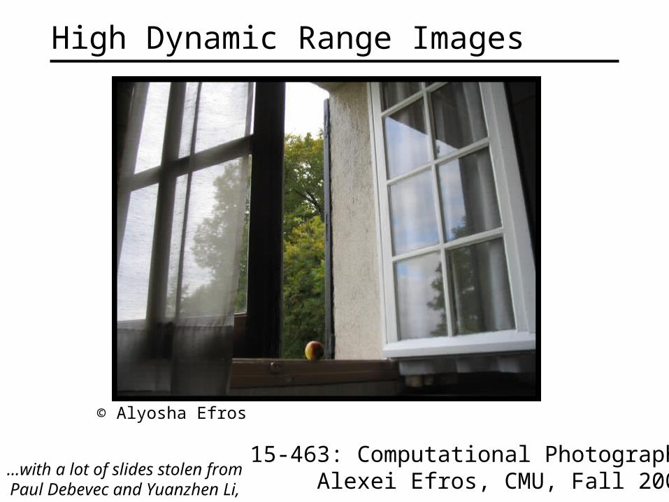
High Dynamic Range Images

15-463: Computational PhotographyAlexei Efros, CMU, Fall 2005

…with a lot of slides stolen from Paul Debevec and Yuanzhen Li,

© Alyosha Efros

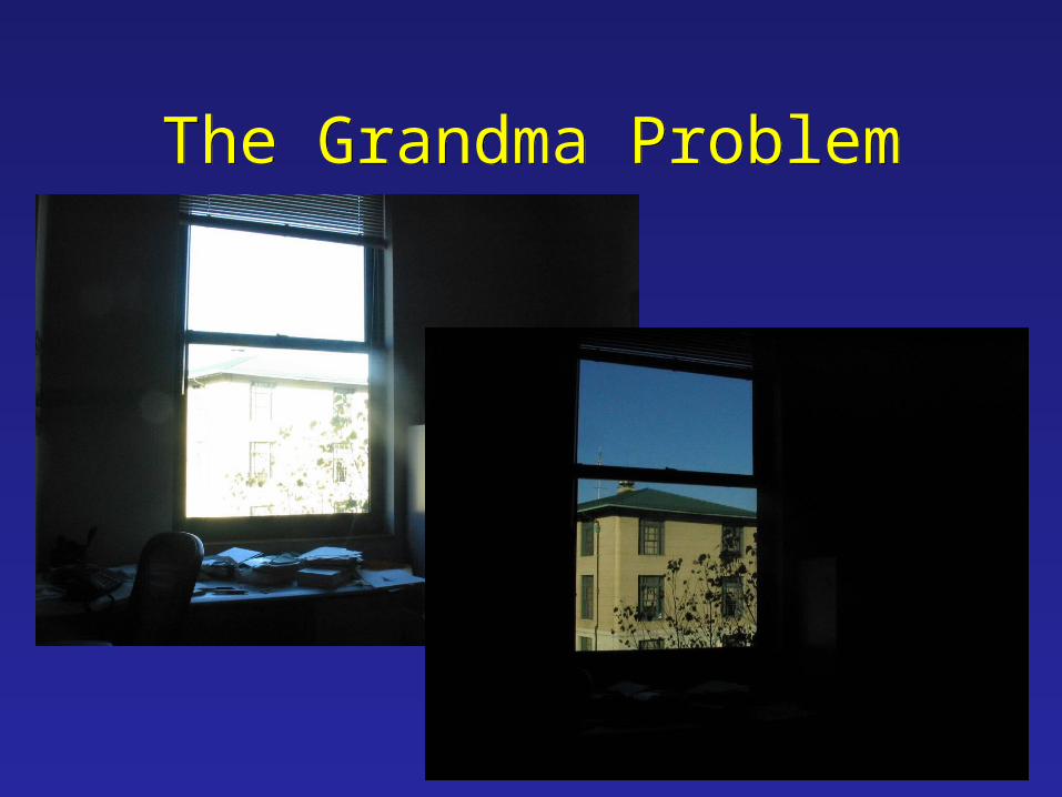
The Grandma ProblemThe Grandma Problem

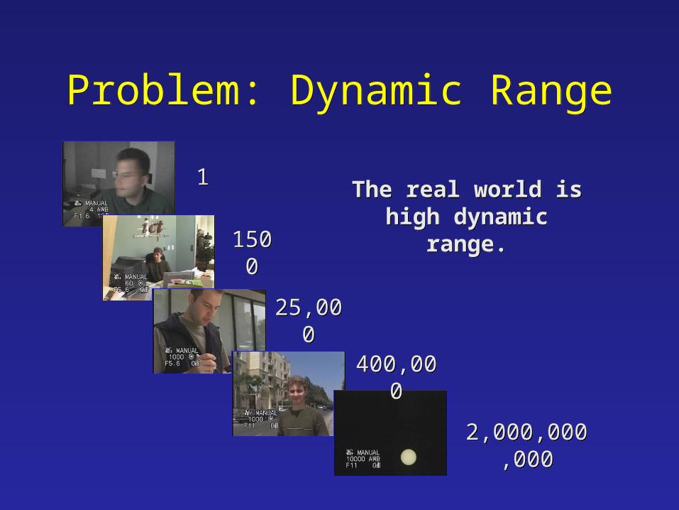
Problem: Dynamic RangeProblem: Dynamic Range

15001500

11

25,00025,000

400,000400,000

2,000,000,0002,000,000,000

The real world ishigh dynamic

range.

The real world ishigh dynamic

range.

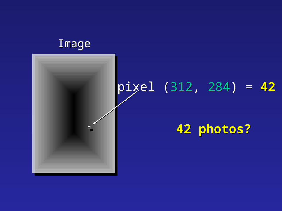
pixel (312, 284) = 42pixel (312, 284) = 42

ImageImage

42 photos?42 photos?

Long ExposureLong Exposure

10-6 106

10-6 106

Real world

Picture

0 to 255

High dynamic range

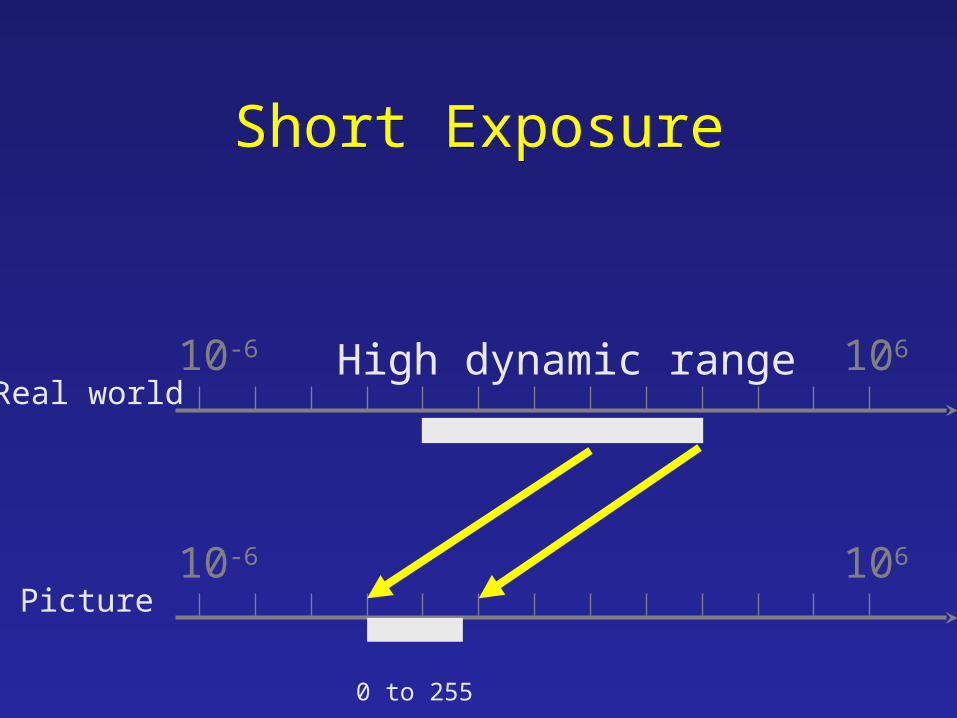
Short ExposureShort Exposure

10-6 106

10-6 106

Real world

Picture

High dynamic range

0 to 255

Camera CalibrationCamera Calibration

• Geometric– How pixel coordinates relate to directions in the

world

• Photometric– How pixel values relate to radiance amounts in

the world

• Geometric– How pixel coordinates relate to directions in the

world

• Photometric– How pixel values relate to radiance amounts in

the world

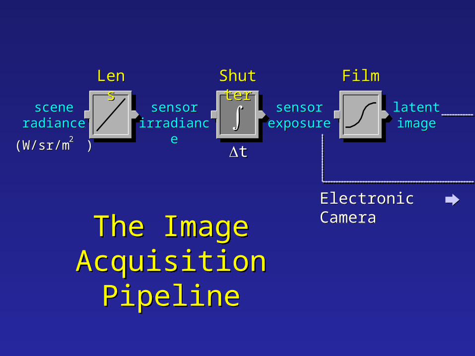
The ImageAcquisition Pipeline

The ImageAcquisition Pipeline

sceneradiance

(W/sr/m )

sceneradiance

(W/sr/m )

sensorirradiance

sensorirradiance

sensorexposuresensor

exposurelatentimagelatentimage

LensLens ShutterShutter FilmFilm

Electronic CameraElectronic Camera

22

tt

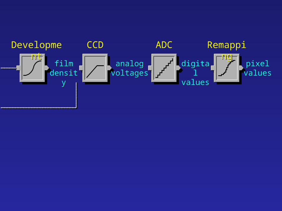
filmdensity

filmdensity

analogvoltagesanalog

voltagesdigitalvaluesdigitalvalues

pixelvaluespixel

values

DevelopmentDevelopment CCDCCD ADCADC RemappingRemapping

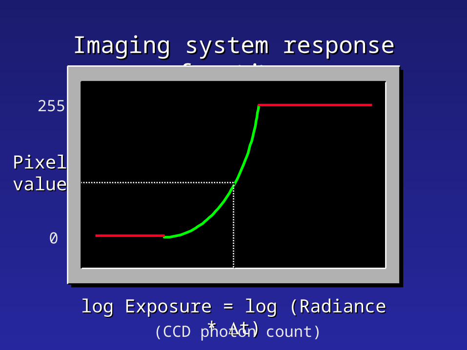
loglog Exposure = Exposure = loglog (Radiance (Radiance * * t)t)

Imaging system response functionImaging system response function

PixelPixelvaluevalue

0

255

(CCD photon count)

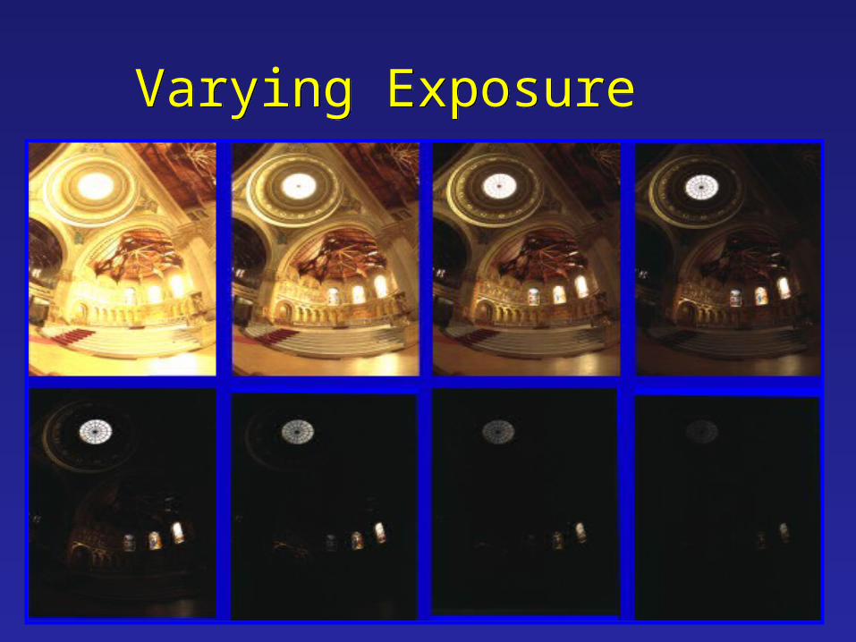
Varying ExposureVarying Exposure

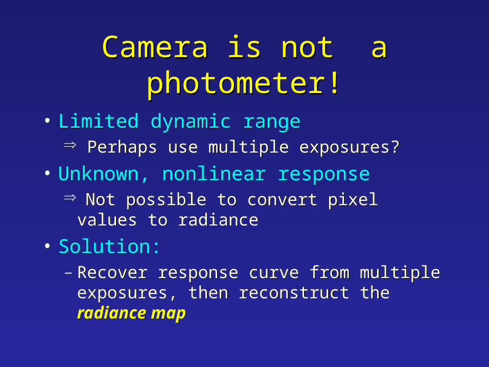
Camera is not a photometer!Camera is not a photometer!

• Limited dynamic range Perhaps use multiple exposures?

• Unknown, nonlinear response Not possible to convert pixel values to

radiance

• Solution:– Recover response curve from multiple

exposures, then reconstruct the radiance map

• Limited dynamic range Perhaps use multiple exposures?

• Unknown, nonlinear response Not possible to convert pixel values to

radiance

• Solution:– Recover response curve from multiple

exposures, then reconstruct the radiance map

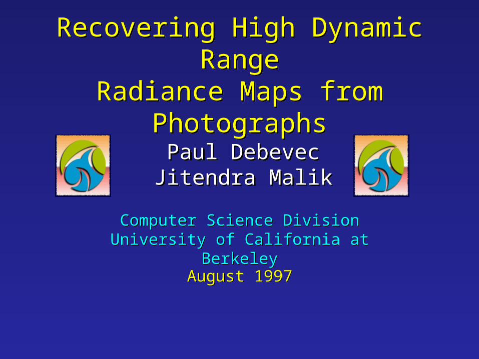
Recovering High Dynamic RangeRadiance Maps from PhotographsRecovering High Dynamic RangeRadiance Maps from Photographs

Paul DebevecJitendra MalikPaul DebevecJitendra Malik

August 1997August 1997

Computer Science DivisionUniversity of California at Berkeley

Computer Science DivisionUniversity of California at Berkeley

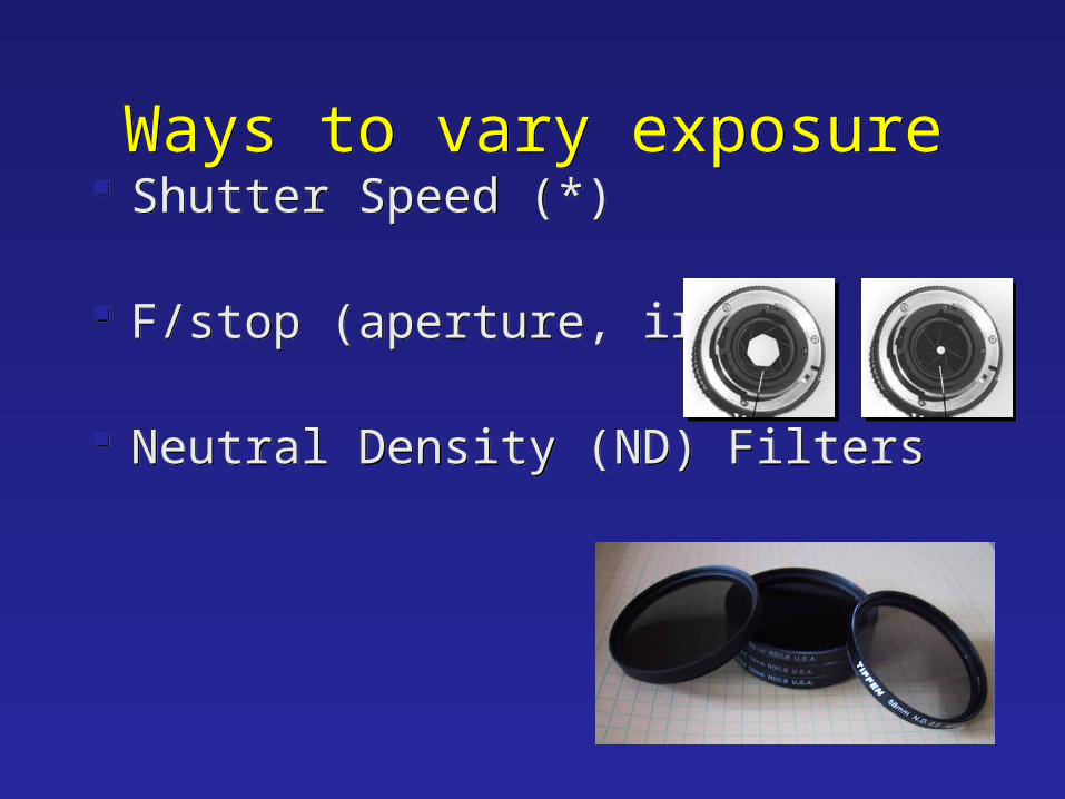
Ways to vary exposureWays to vary exposure Shutter Speed (*)

F/stop (aperture, iris)

Neutral Density (ND) Filters

Shutter Speed (*)

F/stop (aperture, iris)

Neutral Density (ND) Filters

Shutter SpeedShutter Speed

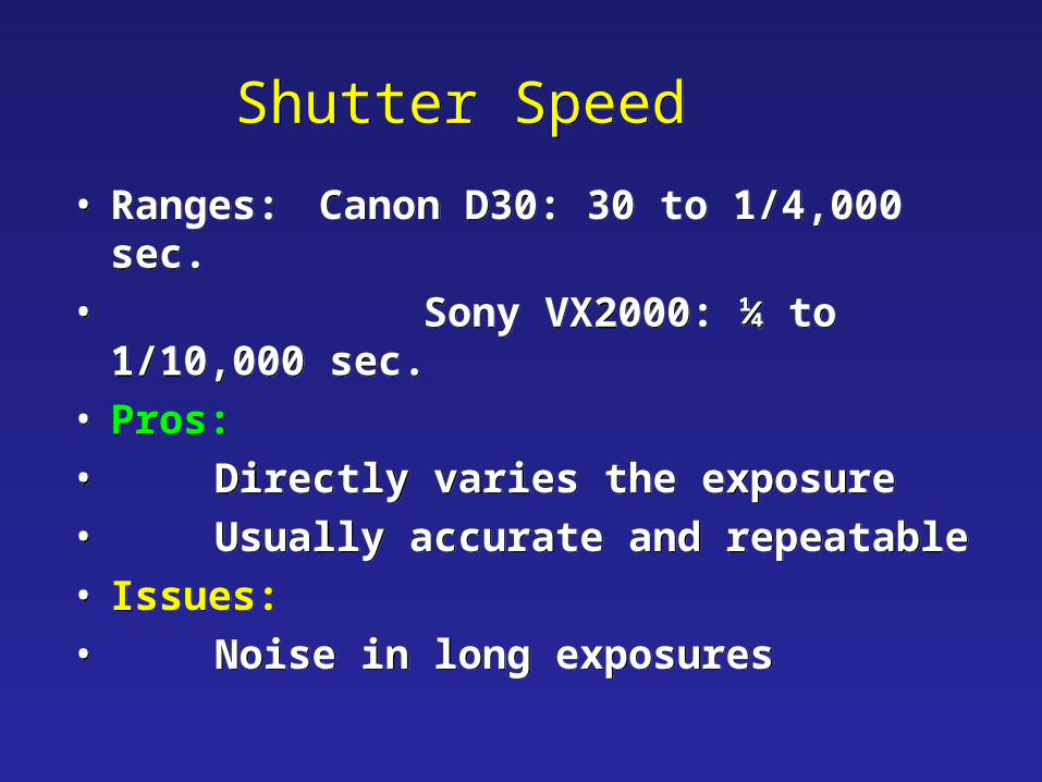
• Ranges: Canon D30: 30 to 1/4,000 sec.• Sony VX2000: ¼ to 1/10,000

sec.• Pros:• Directly varies the exposure• Usually accurate and repeatable• Issues:• Noise in long exposures

• Ranges: Canon D30: 30 to 1/4,000 sec.• Sony VX2000: ¼ to 1/10,000

sec.• Pros:• Directly varies the exposure• Usually accurate and repeatable• Issues:• Noise in long exposures

Shutter SpeedShutter Speed

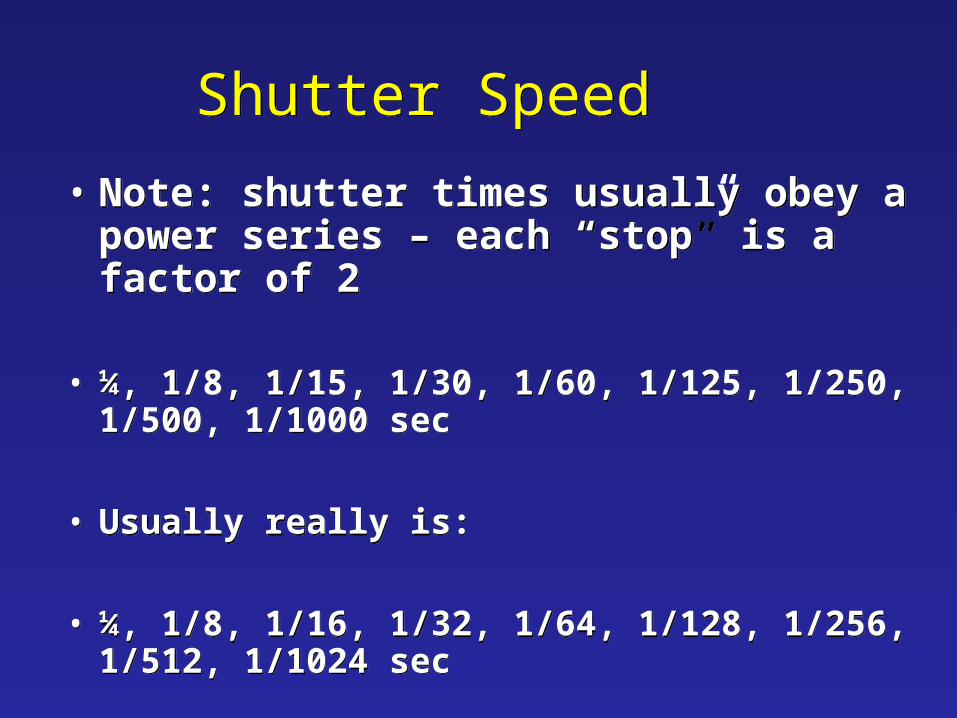
• Note: shutter times usually obey a power series – each “stop” is a factor of 2

• ¼, 1/8, 1/15, 1/30, 1/60, 1/125, 1/250, 1/500, 1/1000 sec

• Usually really is:

• ¼, 1/8, 1/16, 1/32, 1/64, 1/128, 1/256, 1/512, 1/1024 sec

• Note: shutter times usually obey a power series – each “stop” is a factor of 2

• ¼, 1/8, 1/15, 1/30, 1/60, 1/125, 1/250, 1/500, 1/1000 sec

• Usually really is:

• ¼, 1/8, 1/16, 1/32, 1/64, 1/128, 1/256, 1/512, 1/1024 sec

• • 33• • 33

• • 11• • 11 • •

22• • 22

t =t =11 sec sec

• • 33• • 33

• • 11• • 11 • •

22• • 22

t =t =1/16 1/16 secsec

• • 33• • 33

• • 11• • 11

• • 22• • 22

t =t =44 sec sec

• • 33• • 33

• • 11• • 11 • •

22• • 22

t =t =1/64 1/64 secsec

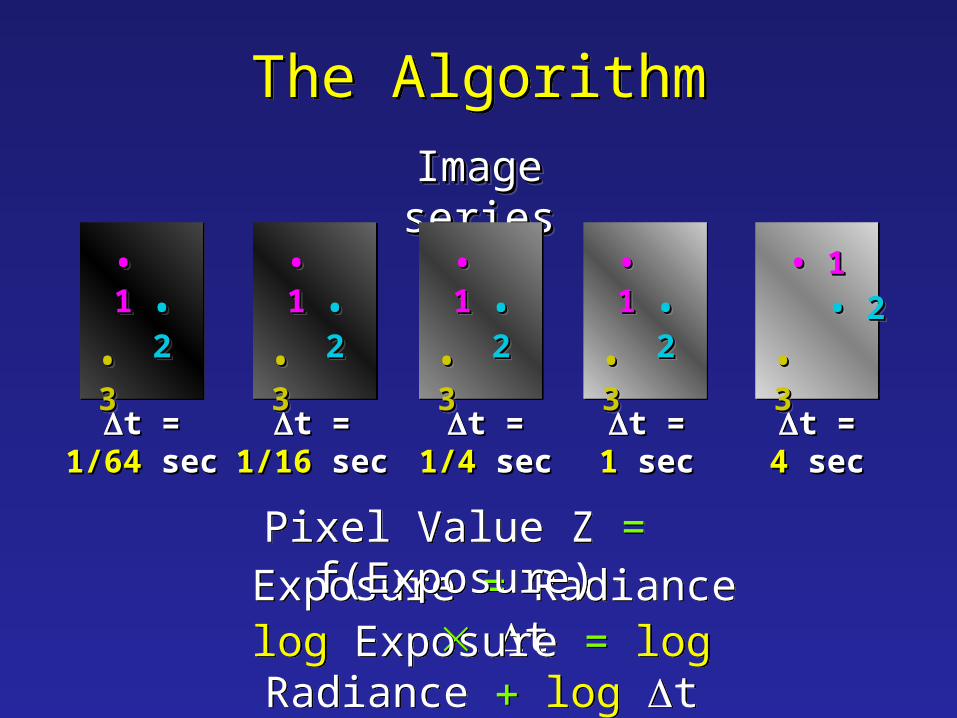
The AlgorithmThe Algorithm

Image seriesImage seriesImage seriesImage series

• • 33• • 33

• • 11• • 11 • •

22• • 22

t =t =1/4 1/4 secsec

Exposure = Radiance tExposure = Radiance tlog Exposure = log Radiance log tlog Exposure = log Radiance log t

Pixel Value Z = f(Exposure)Pixel Value Z = f(Exposure)

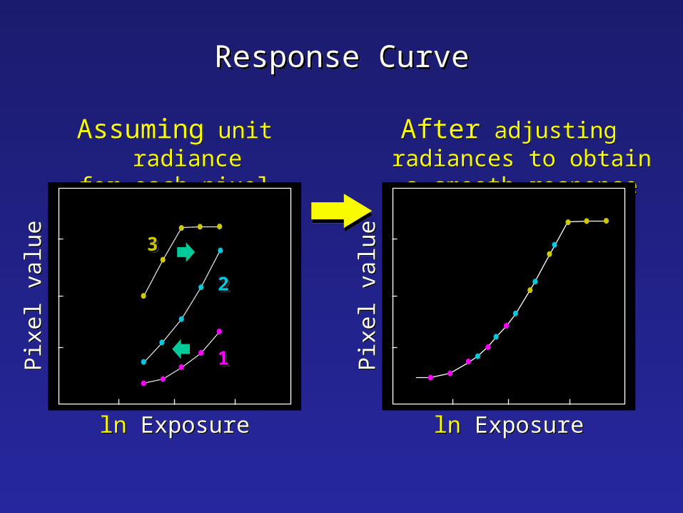
Response CurveResponse Curve

ln Exposureln Exposure

Assuming unit radiancefor each pixel

Assuming unit radiancefor each pixel

After adjusting radiances to obtain a smooth response

curve

After adjusting radiances to obtain a smooth response

curve

Pix

el v

alue

Pix

el v

alue

3333

1111

2222

ln Exposureln Exposure

Pix

el v

alue

Pix

el v

alue

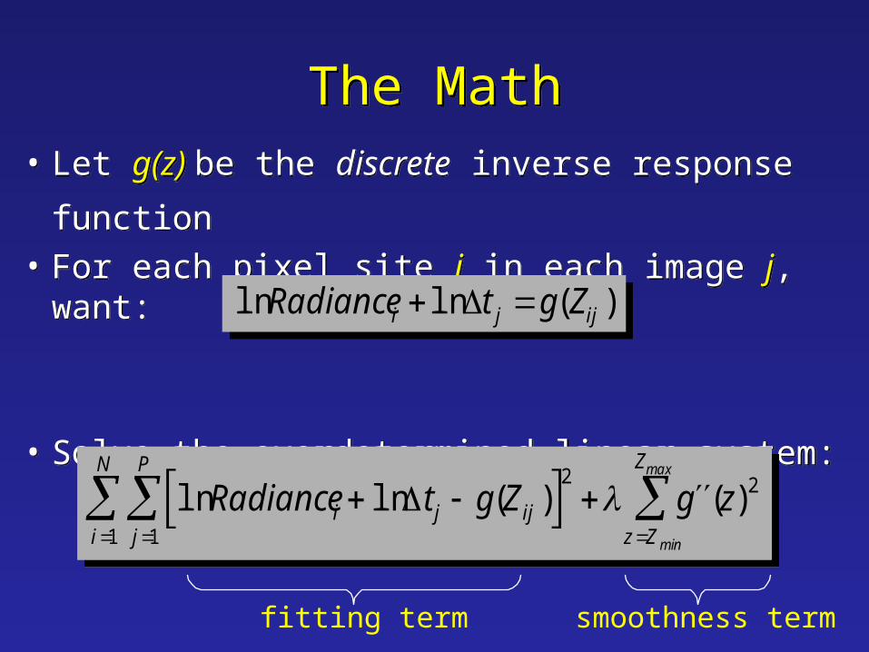
The MathThe Math

• Let g(z) be the discrete inverse response function

• For each pixel site i in each image j, want:

• Solve the overdetermined linear system:

• Let g(z) be the discrete inverse response function

• For each pixel site i in each image j, want:

• Solve the overdetermined linear system:

fitting term smoothness term

ln Radiance i ln t j g(Zij ) 2j 1

P

i 1

N

g (z)2

z Z min

Zmax

ln Radiance i ln t j g(Zij )

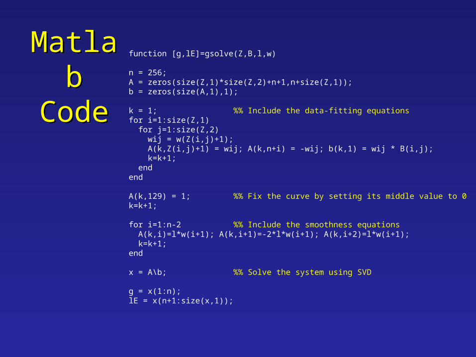
MatlabCode

MatlabCode

function [g,lE]=gsolve(Z,B,l,w)

n = 256;A = zeros(size(Z,1)*size(Z,2)+n+1,n+size(Z,1));b = zeros(size(A,1),1);

k = 1; %% Include the data-fitting equationsfor i=1:size(Z,1) for j=1:size(Z,2) wij = w(Z(i,j)+1); A(k,Z(i,j)+1) = wij; A(k,n+i) = -wij; b(k,1) = wij * B(i,j); k=k+1; endend

A(k,129) = 1; %% Fix the curve by setting its middle value to 0k=k+1;

for i=1:n-2 %% Include the smoothness equations A(k,i)=l*w(i+1); A(k,i+1)=-2*l*w(i+1); A(k,i+2)=l*w(i+1); k=k+1;end

x = A\b; %% Solve the system using SVD

g = x(1:n);lE = x(n+1:size(x,1));

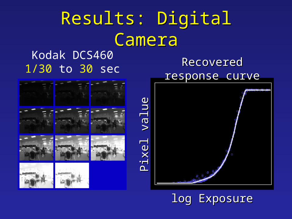
Results: Digital CameraResults: Digital Camera

Recovered response Recovered response curvecurve

log Exposurelog Exposure

Pix

el v

alue

Pix

el v

alue

Kodak DCS4601/30 to 30 sec

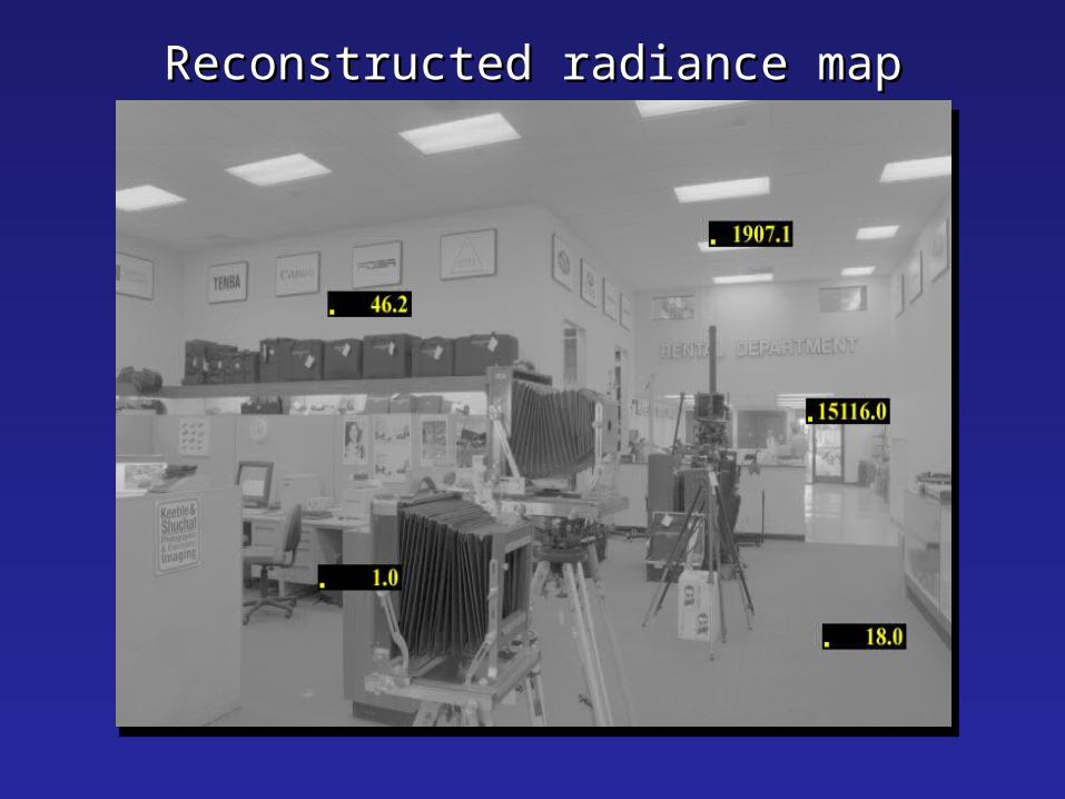
Reconstructed radiance mapReconstructed radiance map

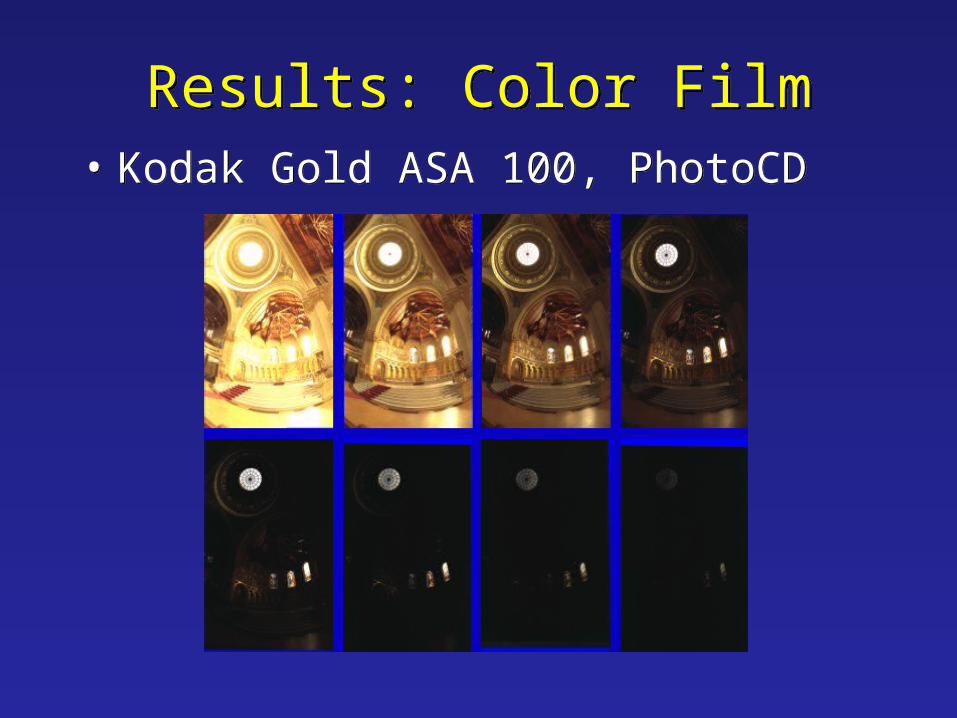
Results: Color FilmResults: Color Film• Kodak Gold ASA 100, PhotoCD• Kodak Gold ASA 100, PhotoCD

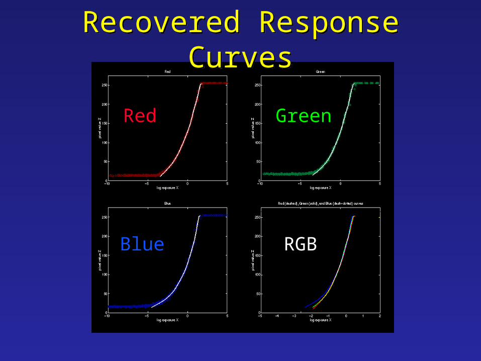
Recovered Response CurvesRecovered Response Curves

Red Green

RGBBlue

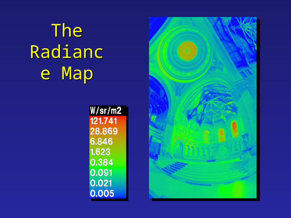
The Radiance

Map

The Radiance

Map

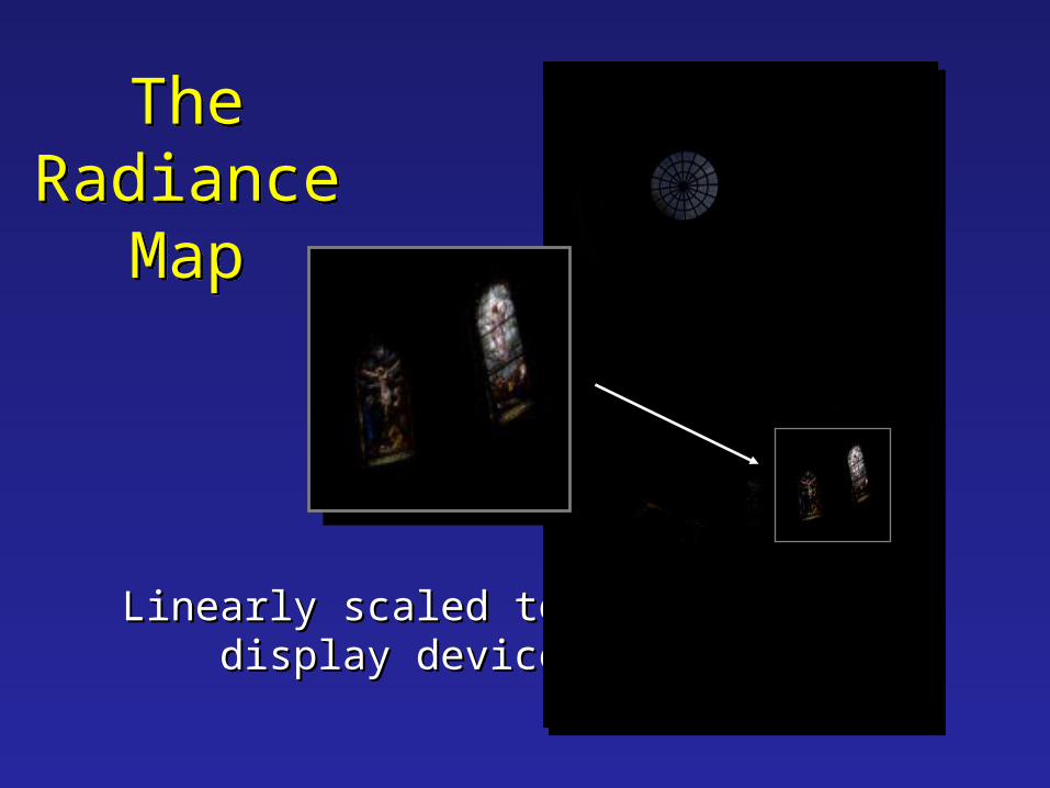
TheRadiance

Map

TheRadiance

Map

Linearly scaled toLinearly scaled todisplay devicedisplay device

Portable FloatMap (.pfm)Portable FloatMap (.pfm)• 12 bytes per pixel, 4 for each channel

sign exponent mantissa

PF768 5121<binary image data>

Floating Point TIFF similarFloating Point TIFF similar

Text header similar to Jeff Poskanzer’s .ppmimage format:

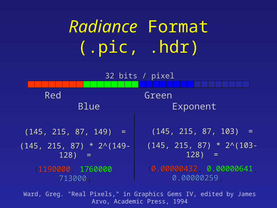
(145, 215, 87, 149) =

(145, 215, 87) * 2^(149-128) =

(1190000, 1760000, 713000)

(145, 215, 87, 149) =

(145, 215, 87) * 2^(149-128) =

(1190000, 1760000, 713000)

Red Green Blue ExponentRed Green Blue Exponent

32 bits / pixel32 bits / pixel

(145, 215, 87, 103) =

(145, 215, 87) * 2^(103-128) =

(0.00000432, 0.00000641, 0.00000259)

(145, 215, 87, 103) =

(145, 215, 87) * 2^(103-128) =

(0.00000432, 0.00000641, 0.00000259)

Ward, Greg. "Real Pixels," in Graphics Gems IV, edited by James Arvo, Academic Press, 1994

Radiance Format(.pic, .hdr)

Radiance Format(.pic, .hdr)

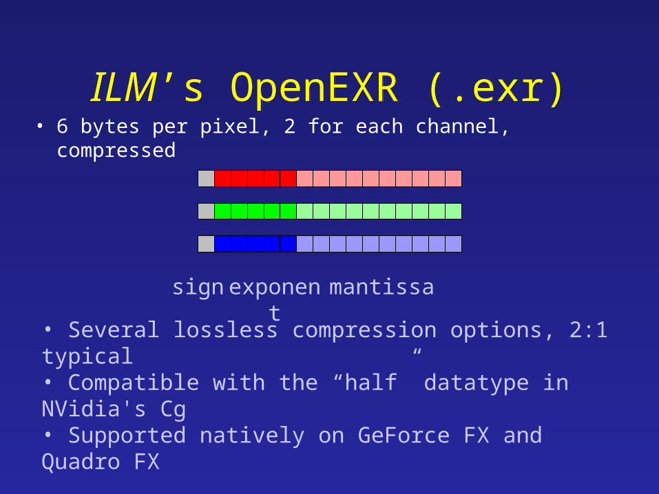
ILM’s OpenEXR (.exr)ILM’s OpenEXR (.exr)• 6 bytes per pixel, 2 for each channel, compressed

sign exponent mantissa

• Several lossless compression options, 2:1 typical• Compatible with the “half” datatype in NVidia's Cg• Supported natively on GeForce FX and Quadro FX

• Available at http://www.openexr.net/

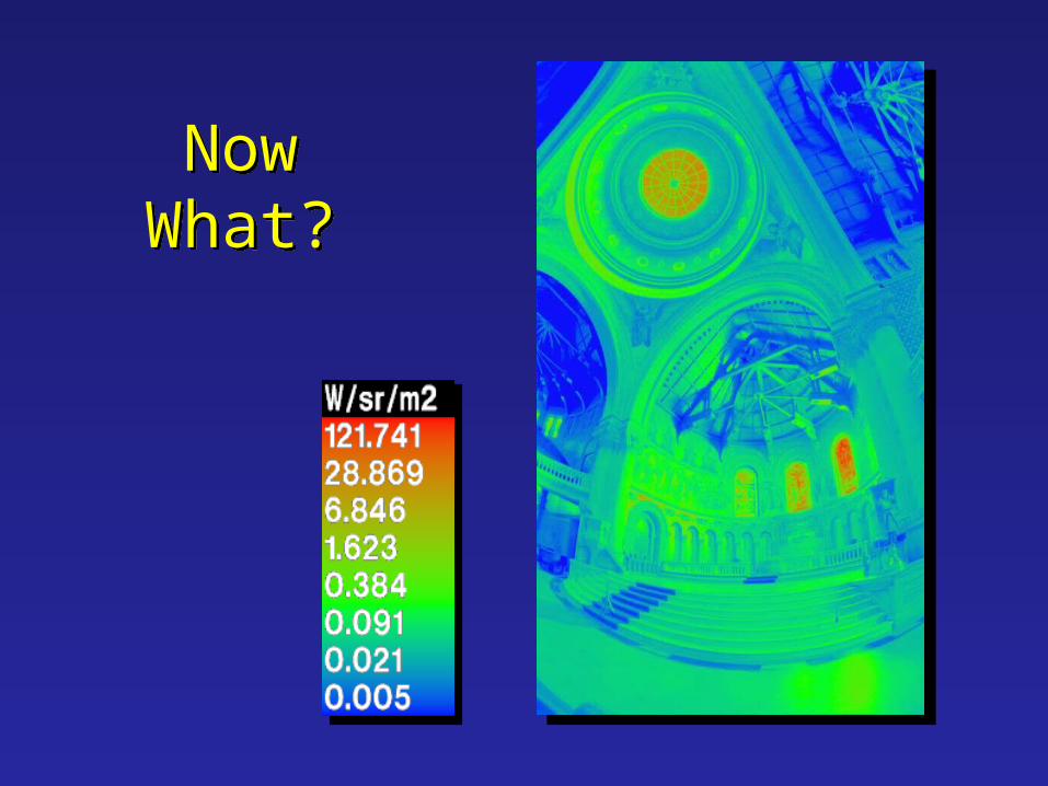
Now What?Now

What?

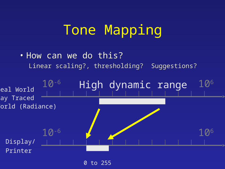
Tone MappingTone Mapping

10-6 106

10-6 106

Real WorldRay Traced World (Radiance)

Display/

Printer

0 to 255

High dynamic range

• How can we do this?Linear scaling?, thresholding? Suggestions?

• How can we do this?Linear scaling?, thresholding? Suggestions?

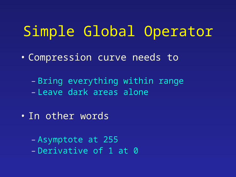
Simple Global OperatorSimple Global Operator

• Compression curve needs to

– Bring everything within range– Leave dark areas alone

• In other words

– Asymptote at 255– Derivative of 1 at 0

• Compression curve needs to

– Bring everything within range– Leave dark areas alone

• In other words

– Asymptote at 255– Derivative of 1 at 0

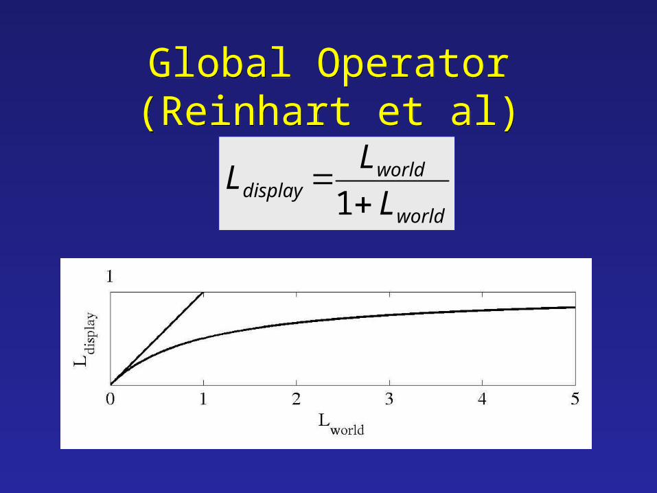
Global Operator (Reinhart et al)Global Operator (Reinhart et al)

world

worlddisplay L

LL

1

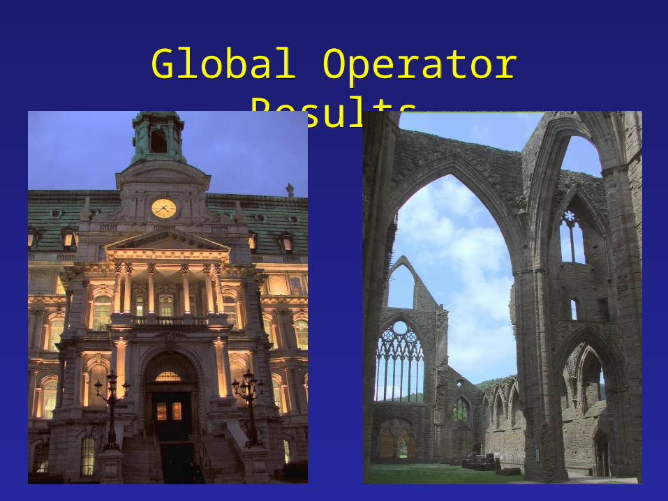
Global Operator ResultsGlobal Operator Results

Darkest Darkest 0.1%0.1% scaled scaledto display deviceto display device

Reinhart OperatorReinhart Operator

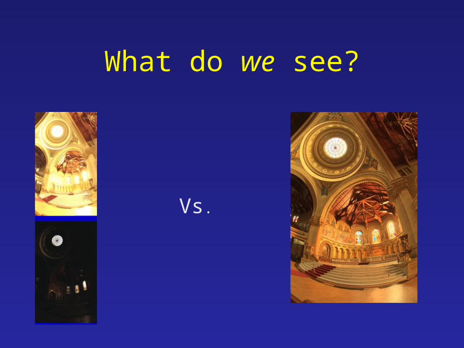
What do we see?What do we see?

Vs.

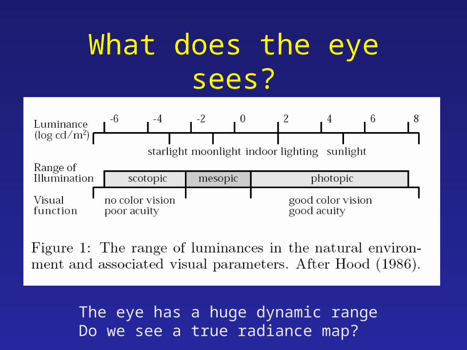
What does the eye sees?What does the eye sees?

The eye has a huge dynamic rangeDo we see a true radiance map?

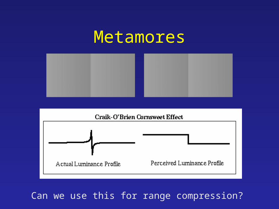
MetamoresMetamores

Can we use this for range compression?

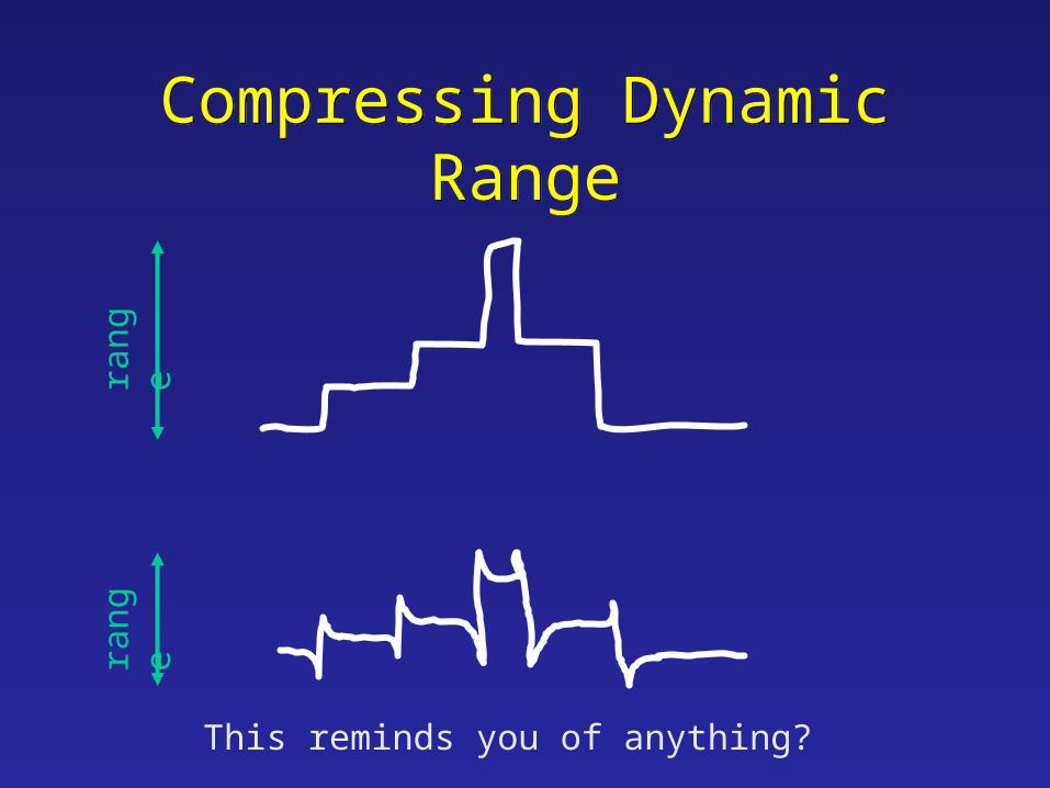
Compressing Dynamic RangeCompressing Dynamic Rangera

nge

rang

e

This reminds you of anything?

Compressing and Companding High Dynamic Range Images with

Subband Architectures

Compressing and Companding High Dynamic Range Images with

Subband Architectures

Yuanzhen Li, Lavanya Sharan, Edward Adelson

Massachusetts Institute of Technology

Dynamic Range ProblemDynamic Range Problem

Source: Shree Nayar

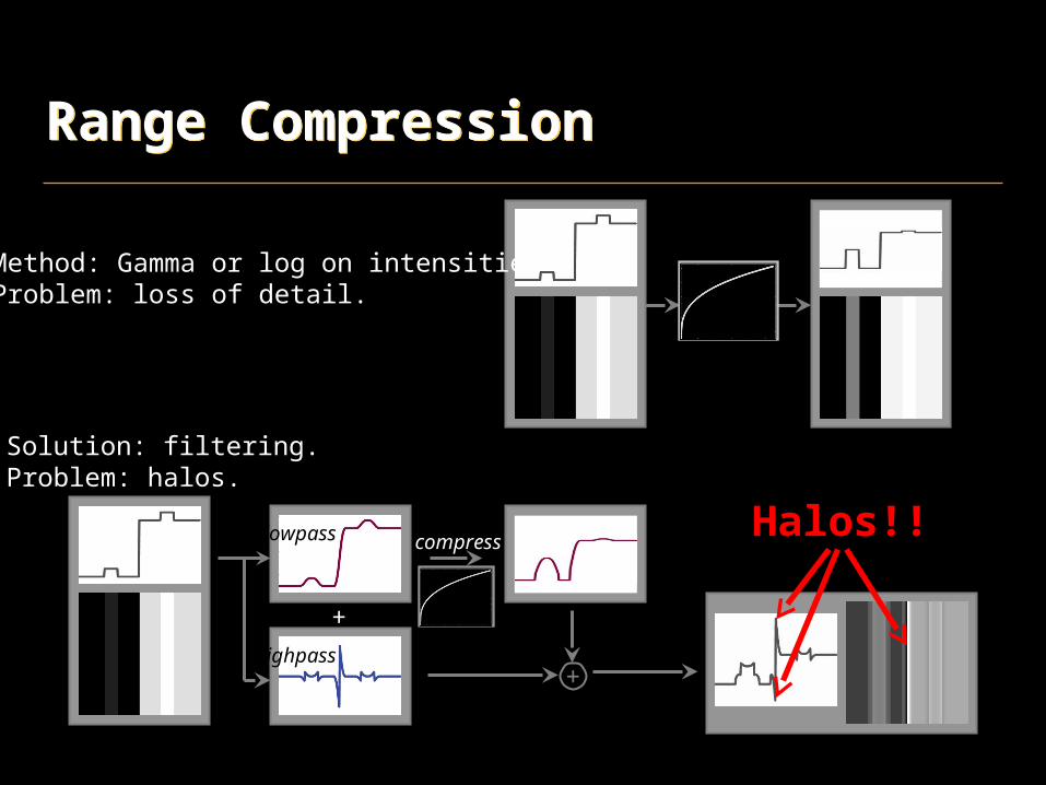
Range CompressionRange Compression

Method: Gamma or log on intensities. Problem: loss of detail.

Solution: filtering.Problem: halos.

+

+

compresslowpass

highpass

Halos!!

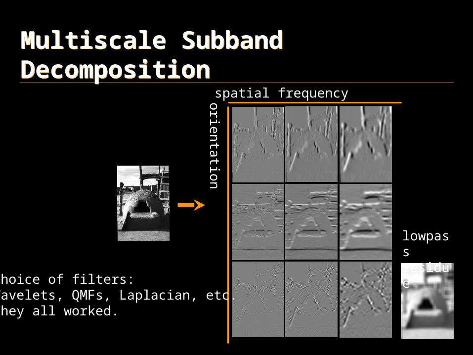
Multiscale Subband DecompositionMultiscale Subband Decomposition

spatial frequency

orie

ntation

lowpass residue

Choice of filters: Wavelets, QMFs, Laplacian, etc.They all worked.

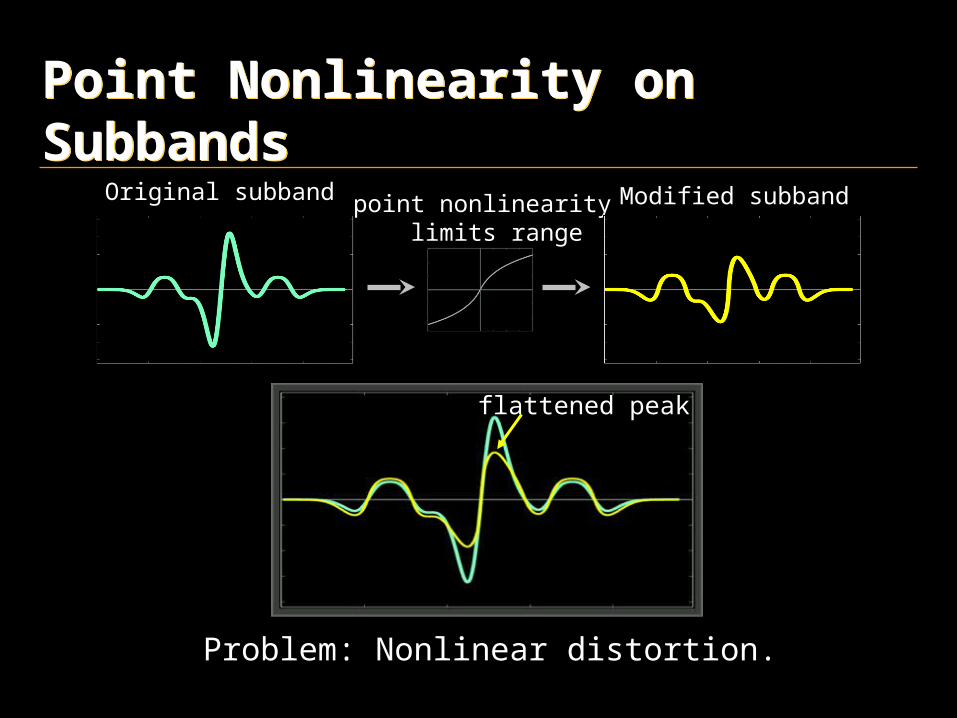
Point Nonlinearity on SubbandsPoint Nonlinearity on Subbands

point nonlinearity limits range

Original subband Modified subband

Problem: Nonlinear distortion.

flattened peak

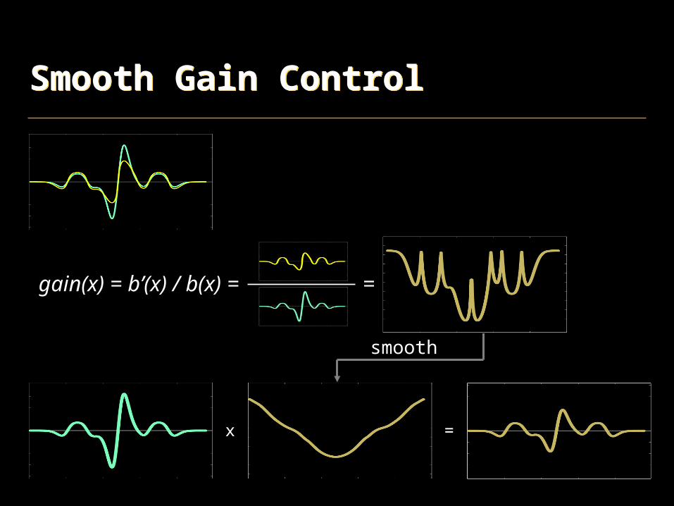
smooth

gain(x) = b’(x) / b(x) = =

Smooth Gain ControlSmooth Gain Control

x =

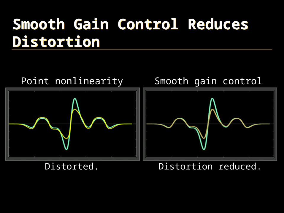
Smooth Gain Control Reduces DistortionSmooth Gain Control Reduces Distortion

Smooth gain controlPoint nonlinearity

Distorted. Distortion reduced.

Smooth Gain Control on SubbandsSmooth Gain Control on Subbands

rectify

blur

activity map gain map

x

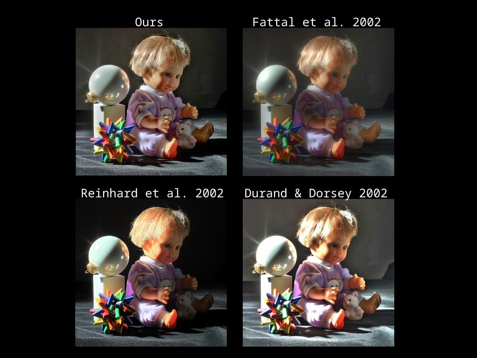
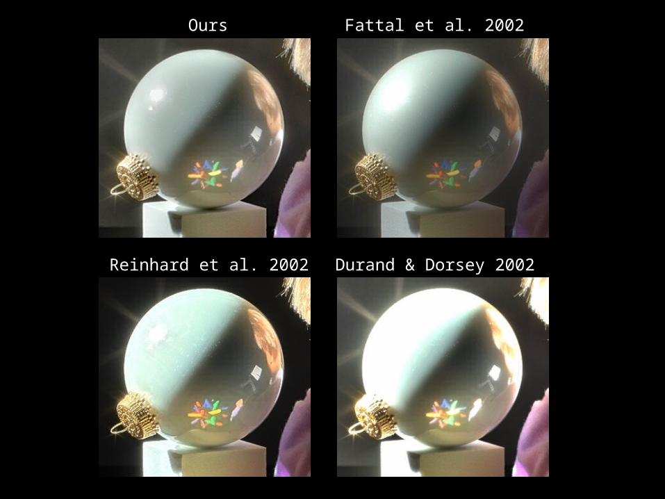
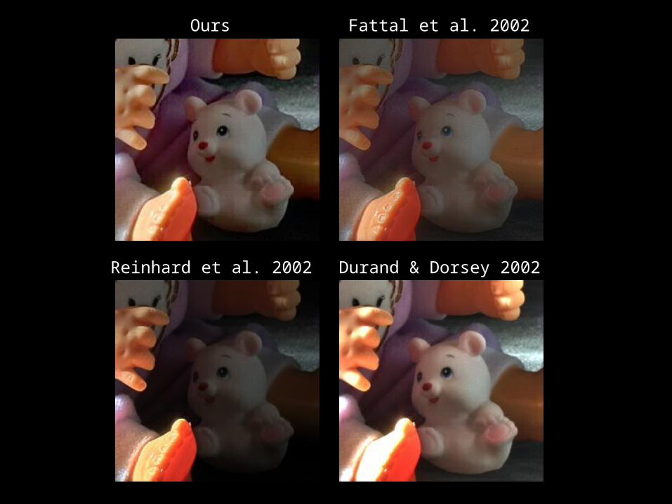
Fattal et al. 2002

Reinhard et al. 2002

Ours

Durand & Dorsey 2002

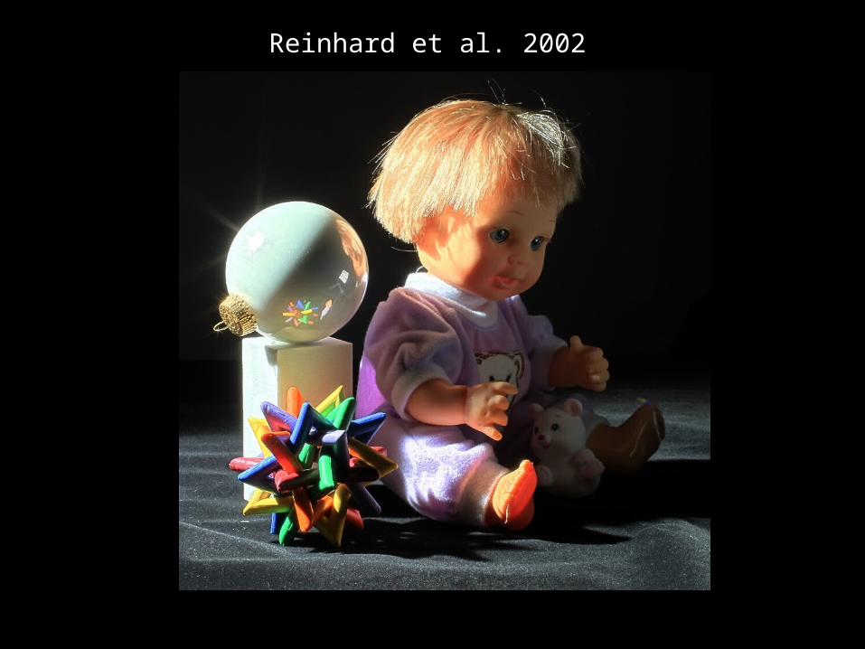
Reinhard et al. 2002

Fattal et al. 2002

Reinhard et al. 2002

Ours

Durand & Dorsey 2002

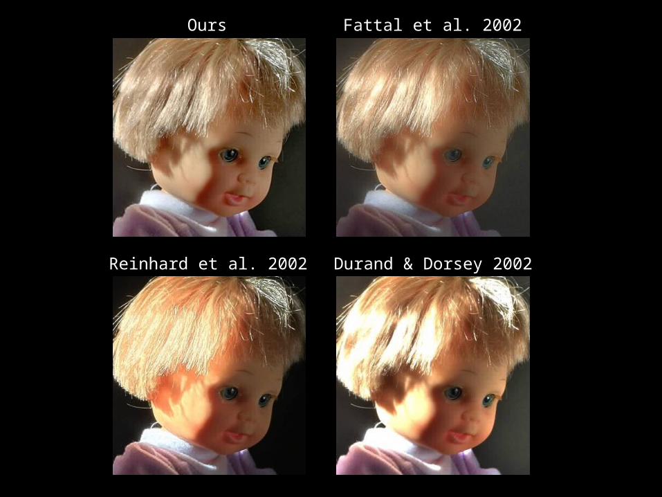
Fattal et al. 2002

Reinhard et al. 2002

Ours

Durand & Dorsey 2002

Fattal et al. 2002

Reinhard et al. 2002

Ours

Durand & Dorsey 2002