Hierarchical Linear Models - University of...

1

Hierarchical Linear Models

Joseph Stevens, Ph.D., University of Oregon(541) 346-2445, [email protected]

© Stevens, 2007

2

Overview and resourcesOverviewWeb site and links: www.uoregon.edu/~stevensj/HLMSoftware:

HLMMLwinNMplusSASR and S-PlusWinBugs

3

Workshop Overview

Preparing dataTwo Level modelsTesting nested hierarchies of modelsEstimationInterpreting resultsThree level modelsLongitudinal modelsPower in multilevel models

4

Hierarchical Data Structures

Many social and natural phenomena have a nested or clustered organization:

Children within classrooms within schoolsPatients in a medical study grouped within doctors within different clinics Children within families within communitiesEmployees within departments within business locations

Grouping and membership in particular units and clusters are important

Grouping and membership in particular units and clusters are important

6

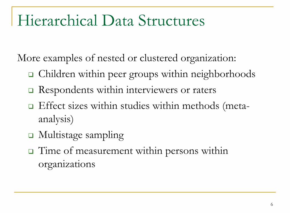
Hierarchical Data Structures

More examples of nested or clustered organization:Children within peer groups within neighborhoodsRespondents within interviewers or ratersEffect sizes within studies within methods (meta-analysis)Multistage samplingTime of measurement within persons within organizations

7

Simpson’s Paradox:

Quiz 1 Quiz 2 Total

Gina 60.0% 10.0% 55.5%

Sam 90.0% 30.0% 35.5%

Clustering Is Important

Well known paradox in which performance of individual groups is reversed when the groups are combined

Quiz 1 Quiz 2 Total

Gina 60 / 100 1 / 10 61 / 110

Sam 9 / 10 30 / 100 39 / 110

8

Simpson’s Paradox: Other Examples2006 US School study:

• In past research, private schools achieve higher than public schools

• Study was expected to provide additional support to the idea that private and charter schools perform better

• USED study (using multilevel modeling):

• Unanalyzed math and reading higher for private schools

• After taking demographic grouping into account, there was littledifference between public and private and differences were almost equally split in favor of each school type

2006 US School study:

• In past research, private schools achieve higher than public schools

• Study was expected to provide additional support to the idea that private and charter schools perform better

• USED study (using multilevel modeling):

• Unanalyzed math and reading higher for private schools

• After taking demographic grouping into account, there was littledifference between public and private and differences were almost equally split in favor of each school type

1975 Berkeley sex bias case:

• UCB sued for bias by women applying to grad school

• Admissions figures showed men more likely to be admitted

• When analyzed by individual department, turned out that no individual department showed a bias; • Women applied to low admission rate departments

• Men applied more to high admission rate departments

1975 Berkeley sex bias case:

• UCB sued for bias by women applying to grad school

• Admissions figures showed men more likely to be admitted

• When analyzed by individual department, turned out that no individual department showed a bias; • Women applied to low admission rate departments

• Men applied more to high admission rate departments

“When the Oakies left Oklahoma and moved to California, it raised the IQ of both states.”

– Will Rogers

“When the Oakies left Oklahoma and moved to California, it raised the IQ of both states.”

– Will Rogers

Participant (i) Cluster (j) Outcome (Y) Predictor (X)

1 1 5 1

2 1 7 3

3 2 4 1

4 2 6 4

5 3 3 3

6 3 5 5

7 4 2 4

8 4 4 6

9 5 1 5

10 5 3 7

Hypothetical Data Example from Snijders & Bosker (1999), n = 2, j=5, nj = N = 10

Hypothetical Data Example from Snijders & Bosker (1999), n = 2, j=5, nj = N = 10

Model Summary

.333a .111 .000 1.826Model1

R R SquareAdjustedR Square

Std. Error ofthe Estimate

Predictors: (Constant), Xa.

Coefficientsa

5.333 1.453 3.671 .006-.333 .333 -.333 -1.000 .347

(Constant)X

Model1

B Std. Error

UnstandardizedCoefficients

Beta

StandardizedCoefficients

t Sig.

Dependent Variable: Ya.

Y = 5.333 -.333(X) + r

Interpretation: There’s a negative relationship between the predictor X and the outcome Y, a one unit increase in X results in .333 lower Y

All 10 cases analyzed without taking cluster membership into account:All 10 cases analyzed without taking cluster membership into account:

X

876543210

Y

8

7

6

5

4

3

2

1

0

Y = 5.333 -.333(X) + rY = 5.333 -.333(X) + r

β0

β1

This is an example of a disaggregated analysis

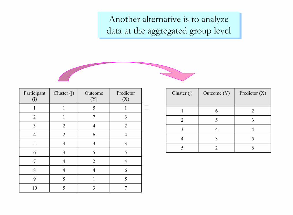
Participant (i)

Cluster (j) Outcome (Y)

Predictor (X)

1 1 5 1

2 1 7 3

3 2 4 2

4 2 6 4

5 3 3 3

6 3 5 5

7 4 2 4

8 4 4 6

9 5 1 5

10 5 3 7

Cluster (j) Outcome (Y) Predictor (X)

1 6 2

2 5 3

3 4 4

4 3 5

5 2 6

Another alternative is to analyze data at the aggregated group levelAnother alternative is to analyze data at the aggregated group level

Y = 8.000 -1.000(X) + r

Interpretation: There’s a negative relationship between the predictor X and the outcome Y, a one unit increase in X results in 1.0 lower Y

The clusters are analyzed without taking individuals into account:The clusters are analyzed without taking individuals into account:

Coefficientsa

8.000 .000 . .-1.000 .000 -1.000 . .

(Constant)MEANX

Model1

B Std. Error

UnstandardizedCoefficients

Beta

StandardizedCoefficients

t Sig.

Dependent Variable: MEANYa.

Model Summary

1.000a 1.000 1.000 .000Model1

R R SquareAdjustedR Square

Std. Error ofthe Estimate

Predictors: (Constant), MEANXa.

This is an example of a disaggregated analysis

Y = 8.000 -1.000(X) + r

MEAN X

76543210

MEA

N Y

8

7

6

5

4

3

2

1

β1

β0

X

876543210

Y

8

7

6

5

4

3

2

1

0

A third possibility is to analyze each cluster separately, looking at the regression relationship within each group

ijr+−+= )XX(00.1YY jijjij

Y = 8.000 -1.000(X) + r

Multilevel regression takes both levels into account:Multilevel regression takes both levels into account:

ijr+−+−= )XX(00.1)X(00.100.8Y jijjij

ijr+−+= )XX(00.1YY jijjij

X

876543210

Y

8

7

6

5

4

3

2

1

0

Taking the multilevel structure of the data into account: Taking the multilevel structure of the data into account:

Within group regressions Between Groups Regression

Total Regression

18

Why Is Multilevel Analysis Needed?

Nesting creates dependencies in the dataDependencies violate the assumptions of traditional statistical models (“independence of error”, “homogeneity of regression slopes”)Dependencies result in inaccurate statistical estimates

Important to understand variation at different levels

19

Decisions About Multilevel Analysis

Properly modeling multilevel structure often matters (and sometimes a lot)Partitioning variance at different levels is useful

tau and sigma (σ 2Y = τ + σ 2)

policy & practice implications

Correct coefficients and unbiased standard errorsCross-level interactionUnderstanding and modeling site or cluster variability

“Randomization by cluster accompanied by analysis appropriate to randomization by individual is an exercise in self-deception and should be discouraged” (Cornfield, 1978, pp.101-2)

20

Preparing Data for HLM Analysis

Use of SPSS as a precursor to HLM assumedHLM requires a different data file for each level in the HLM analysisPrepare data first in SPSS

Clean and screen dataTreat missing dataID variables needed to link levelsSort cases on ID

Then import files into HLM to create an “.mdm” file

21

Creating an MDM file

Example:Go to “Examples” folder and then “Appendix A” in the HLM directoryOpen “HSB1.sav” and “HSB2.sav”

Start HLM and choose “Make new MDM file” from menu; followed

by “Stat package input”

For a two level HLM model stay with the default “HLM2”

Click “Browse”, identify the level 1 data file and open it

Click on “Choose Variables”

Check off the ID linking variable and all variables to

be included in the MDM file

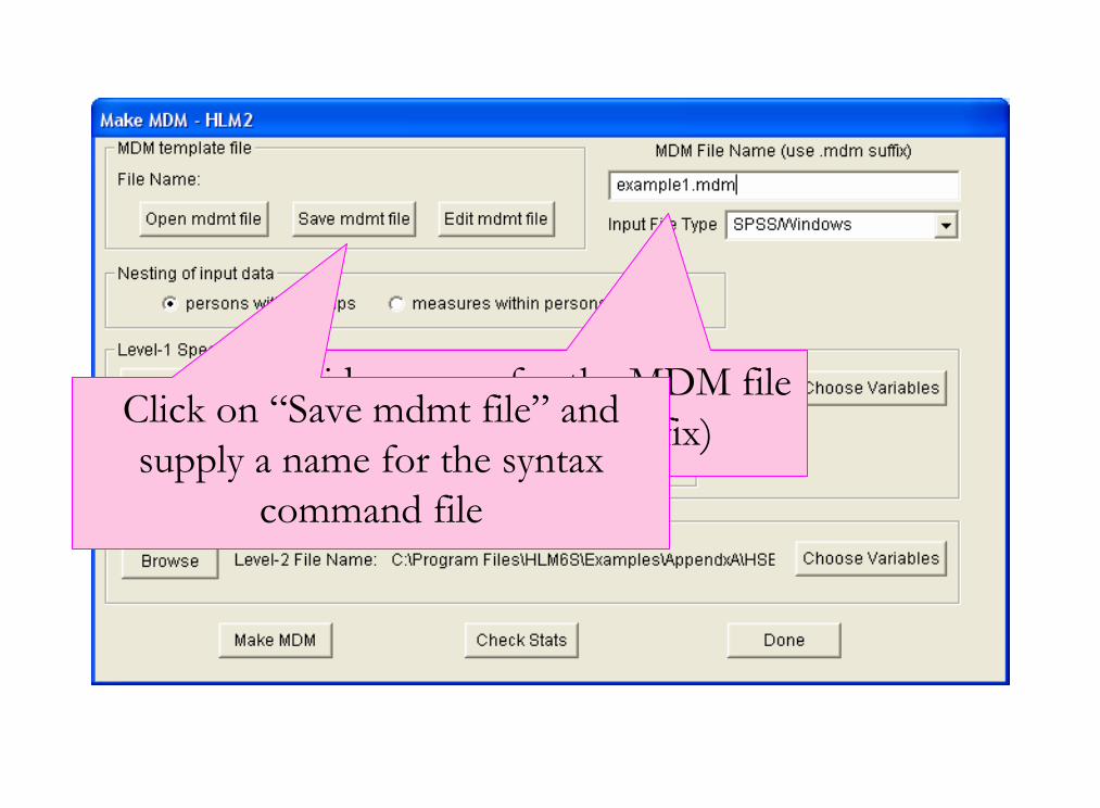
Provide a name for the MDM file (use .mdm as the suffix)Click on “Save mdmt file” and

supply a name for the syntax command file

Click on “Make MDM”

Results will briefly appear

Click on “Check Stats” to see, save, or print results

The click “Done”

You should see a screen like this. You can now begin to specify your HLM model

30

Two-Level HLM Models

31

The Single-Level, Fixed Effects Regression Model

Yi = β0+ β1X1i + β2X2i +…+ βkXki + ri

The parameters βkj are considered fixed One for all and all for oneSame values for all i and j; the single level model

The ri ’s are random: ri ~ N(0, σ) and independent

32

The Multilevel Model

Takes groups into account and explicitly models group effectsHow to conceptualize and model group level variation?How do groups vary on the model parameters?Fixed versus random effects

33

Fixed vs. Random Effects

Fixed Effects represent discrete, purposefully selected or existing values of a variable or factor

Fixed effects exert constant impact on DVRandom variability only occurs as a within subjects effect (level 1)Can only generalize to particular values used

Random Effects represent more continuous or randomly sampled values of a variable or factor

Random effects exert variable impact on DVVariability occurs at level 1 and level 2Can study and model variabilityCan generalize to population of values

34

Fixed vs. Random Effects?

Use fixed effects ifThe groups are regarded as unique entitiesIf group values are determined by researcher through design or manipulationSmall j (< 10); improves power

Use random effects ifGroups regarded as a sample from a larger populationResearcher wishes to test effects of group level variablesResearcher wishes to understand group level differencesSmall j (< 10); improves estimation

35

Fixed Intercepts Model

The simplest HLM model is equivalent to a one-way ANOVA with fixed effects:

Yij = γ00 + rij

This model simply estimates the grand mean (γ00) and deviations from the grand mean (rij)Presented here simply to demonstrate control of fixed and random effects on all parameters

36

Note the equation has no “u” residual term; this creates a fixed effect model

38

ANOVA Model (random intercepts)

A simple HLM model with randomly varying interceptsEquivalent to a one-way ANOVA with random effects:

Yij = β0j + rijβ0j = γ00 + u0j

Yij = γ00 + u0j + rij

Note the addition of u0j allows different intercepts for each j unit, a random effects model

41

ANOVA ModelIn addition to providing parameter estimates, the ANOVA model provides information about the presence of level 2 variance (the ICC) and whether there are significant differences between level 2 unitsThis model also called the Unconditional Model (because it is not “conditioned” by any predictors) and the “empty” modelOften used as a baseline model for comparison to more complex models

42

Variables in HLM Models

Outcome variables Predictors

Control variablesExplanatory variables

Variables at higher levelsAggregated variables (Is n sufficient for representation?)Contextual variables

43

Conditional Models: ANCOVA

Adding a predictor to the ANOVA model results in an ANCOVA model with random intercepts:

Note that the effect of X is constrained to be the same fixed effect for every j unit (homogeneity of regression slopes)

Yij = β0j + β1(X1) + rij

β0j = γ00 + u0j

β1 = γ10

46

Conditional Models: Random Coefficients

An additional parameter results in random variation of the slopes:

Both intercepts and slopes now vary from group to group

Yij = β0j + β1(X1) + rij

β0j = γ00 + u0j

β1j = γ10 + u1j

49

Standardized coefficients

Standardized coefficient at level 1:β0j (SDX / SDY)

Standardized coefficient at level 2:γ00 (SDX / SDY)

50

Modeling variation at Level 2:Intercepts as Outcomes

Yij = β0j + β1jX1ij + rij

β0j = γ00 + γ0jWj + u0j

β1j = γ10 + u1j

Predictors (W’s) at level 2 are used to model variation in intercepts between the j units

51

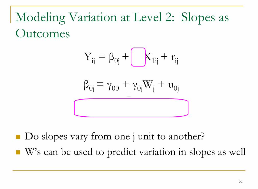
Modeling Variation at Level 2: Slopes as Outcomes

Yij = β0j + β1jX1ij + rij

β0j = γ00 + γ0jWj + u0j

β1j = γ10 + γ1jWj + u1j

Do slopes vary from one j unit to another?W’s can be used to predict variation in slopes as well

52

Variance Components Analysis

VCA allows estimation of the size of random variance components

Important issue when unbalanced designs are usedIterative procedures must be used (usually ML estimation)

Allows significance testing of whether there is variation in the components across units

53

Estimating Variance Components: Unconditional Model

= τ0 + σ2

Var(Yij) = Var(u0j) + Var(rij)

54

Final estimation of variance components:---------------------------------------------------------------------------------------------------Random Effect Standard Variance df Chi-square P-value

Deviation Component---------------------------------------------------------------------------------------------------INTRCPT1, U0 14.38267 206.86106 14 457.32201 0.000level-1, R 32.58453 1061.75172---------------------------------------------------------------------------------------------------

Statistics for current covariance components model--------------------------------------------------Deviance = 21940.853702Number of estimated parameters = 2

HLM Output

55

Variance explained

R2 at level 1 = 1 – (σ2

cond + τcond) / (σ2uncond + τuncond)

R2 at level 2 = 1 – [(σ2

cond / nh) + τcond] / [(σ2uncond / nh) + τuncond]

Where nh = the harmonic mean of n for the level 2 units (k / [1/n1 + 1/n2 +…1/nk])

56

Comparing models

Deviance testsUnder “Other Settings” on HLM tool bar, choose “hypothesis testing”Enter deviance and number of parameters from baseline model

Variance explainedExamine reduction in unconditional model variance as predictors added, a simpler level 2 formula:

R2 = (τ baseline – τ conditional) / τ baseline

58

Deviance Test Results

Statistics for current covariance components model------------------------------------------------------------Deviance = 21615.283709Number of estimated parameters = 2

Variance-Covariance components test------------------------------------------------------------Chi-square statistic = 325.56999Number of degrees of freedom = 0P-value = >.500

59

Testing a Nested Sequence of HLM Models1. Test unconditional model2. Add level 1 predictors

Determine if there is variation across groups If not, fix parameterDecide whether to drop nonsignificant predictorsTest deviance, compute R2 if so desired

3. Add level 2 predictorsEvaluate for significanceTest deviance, compute R2 if so desired

60

Example

Use the HSB MDM file previously created to practice running HLM models:

UnconditionalLevel 1 predictor fixed, then randomLevel 2 predictor

61

Statistical Estimation in HLM Models

Estimation MethodsFMLRMLEmpirical Bayes estimation

Parameter estimation Coefficients and standard errorsVariance Components

Parameter reliabilityCenteringResidual files

62

Estimation Methods: Maximum Likelihood Estimation (MLE) Methods

MLE estimates model parameters by estimating a set of population parameters that maximize a likelihood functionThe likelihood function provides the probabilities of observing the sample data given particular parameter estimatesMLE methods produce parameters that maximize the probability of finding the observed sample data

63

Estimation Methods

Full: Simultaneously estimate the fixed effects and the variance components.

Goodness of fit statistics apply to the entire model

(both fixed and random effects)

Check on software default

Full: Simultaneously estimate the fixed effects and the variance components.

Goodness of fit statistics apply to the entire model

(both fixed and random effects)

Check on software default

Restricted: Sequentially estimates the fixed effects and then the variance components

Goodness of fit statistics (deviance tests) apply only to the random effects

RML only tests hypotheses about the VCs (and the models being compared must have identical fixed effects)

Restricted: Sequentially estimates the fixed effects and then the variance components

Goodness of fit statistics (deviance tests) apply only to the random effects

RML only tests hypotheses about the VCs (and the models being compared must have identical fixed effects)

RML – Restricted Maximum Likelihood, only the variance components are included in the likelihood function

RML – Restricted Maximum Likelihood, only the variance components are included in the likelihood functionFML – Full Maximum Likelihood, both the regression coefficients and the variance components are included in the likelihood function

FML – Full Maximum Likelihood, both the regression coefficients and the variance components are included in the likelihood function

64

Estimation Methods

RML expected to lead to better estimates especially when j is smallFML has two advantages:

Computationally easierWith FML, overall chi-square tests both regression coefficients and variance components, with RML only variance components are testedTherefore if fixed portion of two models differ, must use FML for nested deviance tests

65

Computational Algorithms

Several algorithms exist for existing HLM models:Expectation-Maximization (EM)Fisher scoringIterative Generalized Least Squares (IGLS)Restricted IGLS (RIGLS)

All are iterative search and evaluation procedures

66

Model Estimation

Iterative estimation methods usually begin with a set of start valuesStart values are tentative values for the parameters in the model

Program begins with starting values (usually based on OLS regression at level 1)Resulting parameter estimates are used as initial values for estimating the HLM model

67

Model EstimationStart values are used to solve model equations on first iterationThis solution is used to compute initial model fitNext iteration involves search for better parameter valuesNew values evaluated for fit, then a new set of parameter values triedWhen additional changes produce no appreciable improvement, iteration process terminates (convergence)Note that convergence and model fit are very different issues

IntermissionIntermission

69

Centering

No centering (common practice in single level regression)Centering around the group mean ( )Centering around the grand mean (M )A known population meanA specific meaningful time point

jX

70

Centering: The Original Metric

Sensible when 0 is a meaningful point on the original scale of the predictor

For example, amount of training ranging from 0 to 14 daysDosage of a drug where 0 represents placebo or no treatment

Not sensible or interpretable in many other contexts, i.e. SAT scores (which range from 200 to 800)

71

0 10 20 30 40 50

)0(0 == ijijj XYEβ

72

Centering Around the Grand Mean

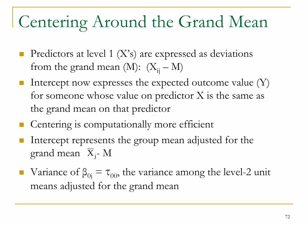
Predictors at level 1 (X’s) are expressed as deviations from the grand mean (M): (Xij – M)Intercept now expresses the expected outcome value (Y) for someone whose value on predictor X is the same as the grand mean on that predictorCentering is computationally more efficientIntercept represents the group mean adjusted for the grand mean - M

Variance of β0j = τ00, the variance among the level-2 unit means adjusted for the grand mean

jX

73

0 10 20 30 40 50

) ( 000 γβ == ijijj XYE

Centering Around the Grand Mean

β01

β02

β03

74

Centering Around the Group Mean

Individual scores are interpreted relative to their group mean The individual deviation scores are orthogonal to the group meansIntercept represents the unadjusted mean achievement for the groupUnbiased estimates of within-group effects May be necessary in random coefficient models if level 1 predictor affects the outcome at both level 1 and level 2Can control for unmeasured between group differencesBut can mask between group effects; interpretation is more complex

)( XXij −

75


Level 1 results are relative to group membership

Intercept becomes the unadjusted mean for group j

Should include level 2 mean of level 1 variables to fully disentangle individual and compositional effects

Variance β0j is now the variance among the level 2 unit means

76

0 10 20 30 40 50

)25 ( then 25, X If 11011 === ii XYEβ


)20 ( then 20, X If 22022 === ii XYEβ)18 ( then 18, X If 33033 === ii XYEβ

77

Parameter estimation

Coefficients and standard errors estimated through maximum likelihood procedures (usually)

The ratio of the parameter to its standard error produces a Wald test evaluated through comparison to the normal distribution (z)In HLM software, a more conservative approach is used:

t-tests are used for significance testing t-tests more accurate for fixed effects, small n, and nonnormal distributions)

Standard errorsVariance components

78

Parameter reliability

Analogous to score reliability: ratio of true score variance to total variance (true score + error)In HLM, ratio of true parameter variance to total variabilityFor example, in terms of intercepts, parameter reliability, λ, is:

)//()(/)( 2200

2000 jjjj nYVarVar σττβλ +==

Total variance of the sample means (observed)

True variance of the sample means (estimated)

Variance of error of the sample meansTrue variance of the

sample means (estimated)

79

ICC ( ρI )

nj .05 .10 .20

5 .21 .36 .56

10 .34 .53 .71

20 .51 .69 .83

30 .61 .77 .88

50 .72 .85 .93

100 .84 .92 .96

)1(1

Ij

Ijj n

nρ

ρλ

−+=


80


)1(1

Ij

Ijj n

nρ

ρλ

−+=

n per cluster

100503020105

Para

met

er R

elia

bilit

y1.0

.8

.6

.4

.2

0.0

ICC=.05

ICC=.10

ICC=.20

81

Predicting Group Effects

It is often of interest to estimate the random group effects (β0j, β1j)This is accomplished using Empirical Bayes (EB) estimationThe basic idea of EB estimation is to predict group values using two kinds of information:

Group j dataPopulation data obtained from the estimation of the regression model

82

Empirical Bayes

If information from only group j is used to estimate then we have the OLS estimate:

If information from only the population is used to estimate then the group is estimated from the grand mean:

j

N

j

j YNn

Y 1

..00 ∑=

==γ

jj Y=0β

83

Empirical Bayes

A third possibility is to combine group level and population informationThe optimal combination is an average weighted the parameter reliability:

The results in the “posterior means” or EB estimates

0000 )1( γλβλβ jjjjEB −+=

The larger the reliability, the greater the weight of the group mean

The smaller the reliability, the greater the weight of the grand mean

84

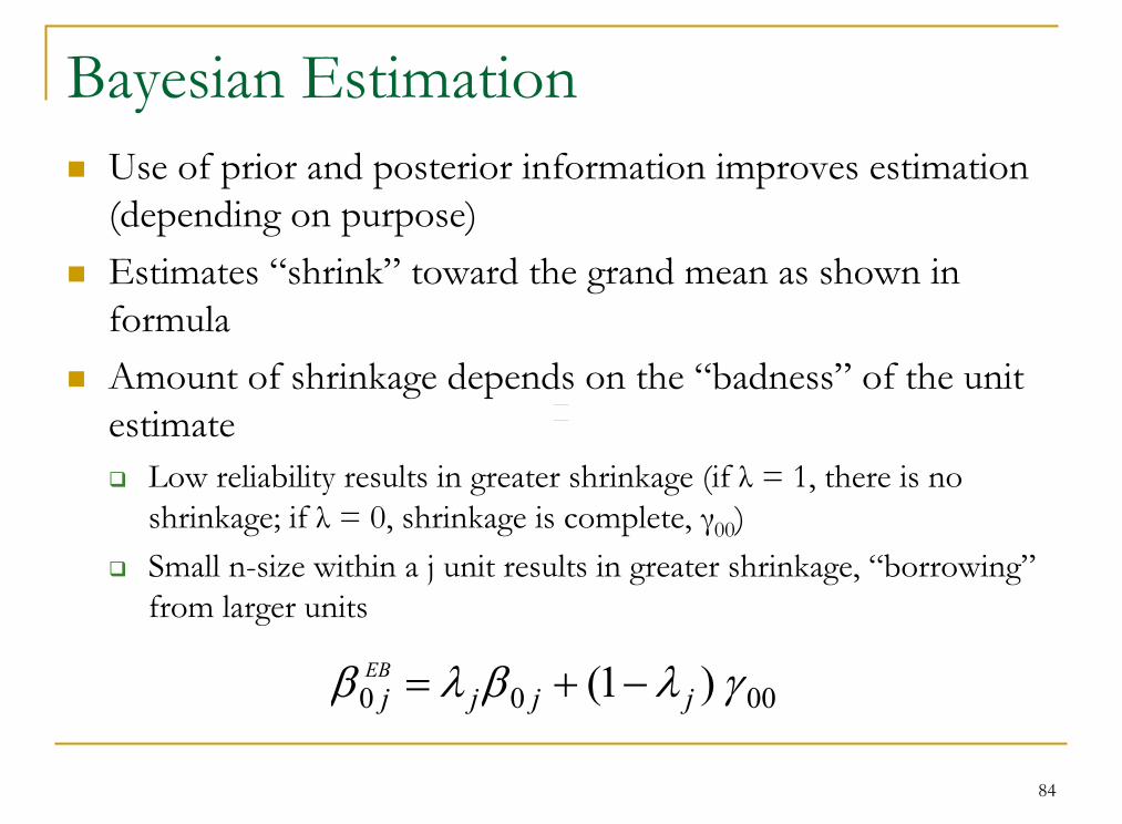
Bayesian EstimationUse of prior and posterior information improves estimation (depending on purpose)Estimates “shrink” toward the grand mean as shown in formulaAmount of shrinkage depends on the “badness” of the unit estimate

Low reliability results in greater shrinkage (if λ = 1, there is no shrinkage; if λ = 0, shrinkage is complete, γ00)Small n-size within a j unit results in greater shrinkage, “borrowing”from larger units

0000 )1( γλβλβ jjjjEB −+=

OLS Intercept

201816141210864

EB In

terc

ept

20

18

16

14

12

10

8

6

4 Rsq = 0.9730

Reliability=.733

OLS Slope

86420-2-4

EB S

lope

4

3

2

1

0 Rsq = 0.3035

Reliability=.073

High School

Achi

evem

ent

22

17

12

7

2

EB

OLS

87

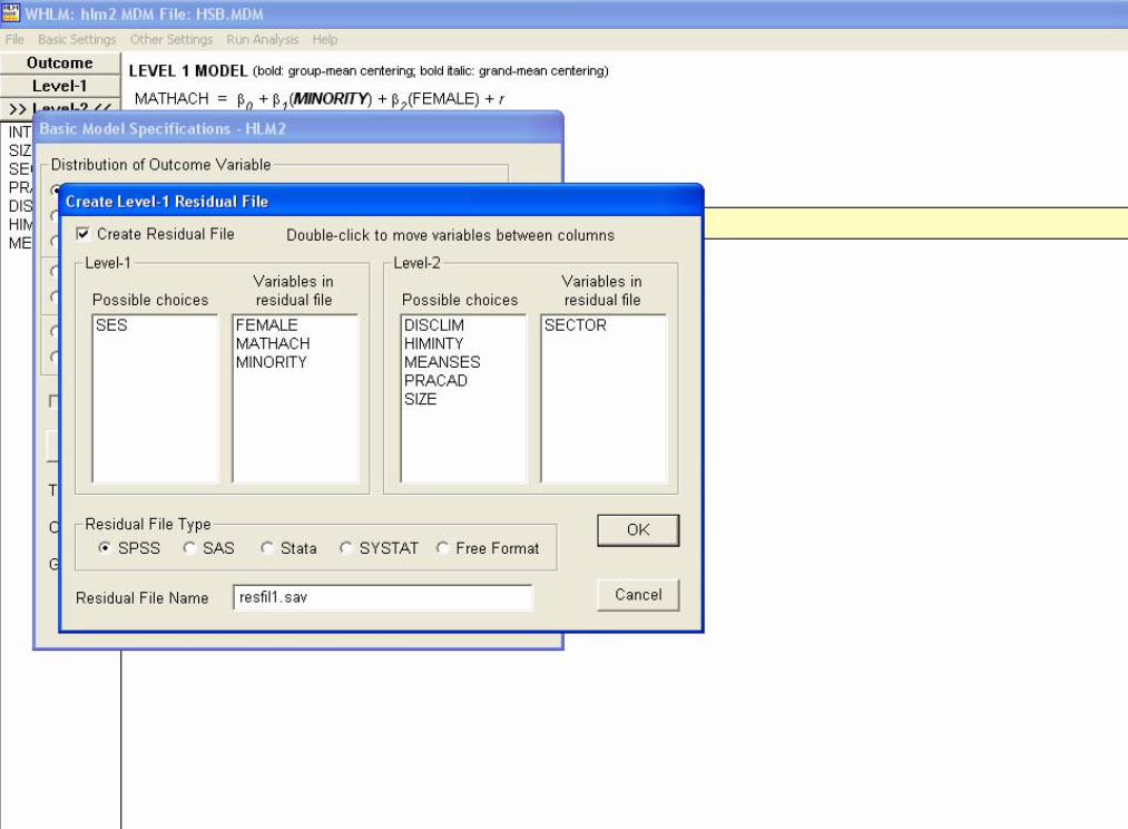
HLM Residual FilesImportant outcome information from an HLM analysis can be saved for each level of the analysis in a “residual file”

Residual files contain parameter estimates and other variables from the analysisResidual files can be save in statistical package format (SPSS, SAS, etc.)

Residual files can be used for diagnostic evaluation of statistical model assumptionsResidual files can be used to estimate and further describe or analyze effects among the units at each level

95

Example: Creating Residual Files

96

Three level modelsLevel-1 (p students)

Yijk = π0jk + π1jk(apijk)+ eijkLevel-2 (j classrooms)

π0jk = βp0k + βp1k(Xqjk) + rp0k

π1jk = βp1kj + βp1k(Xqjk) + rp1kLevel-3 (k schools)

βp0k = γpq0 + γpqs(Wsk) + upqk

βp1k = γpq1 + γpqs(Wsk) + upqk

97

Partitioning variance in the three level modelProportion of variance within classrooms (individual

student differences) = σ2 / (σ2 + τπ + τβ )

Proportion of variance between classrooms within schools = τπ / (σ2 + τπ + τβ )

Proportion of variance between schools = τβ / (σ2 + τπ + τβ )

98

Three level example

Example:Go to “Examples” folder and then “Chapter 4” in the HLM directoryOpen “EG1.sav”, “EG2.sav”, and “EG3.sav”

99

Longitudinal modelsLevel 1 defined as repeated measurement occasionsLevels 2 and 3 defined as higher levels in the nested structureFor example, longitudinal analysis of student achievement

Level 1 = achievement scores at times 1 – tLevel 2 = student characteristicsLevel 3 = school characteristics

100

Longitudinal models

Two important advantages of the MLM approach to repeated measures:

Times of measurement can vary from one person to anotherData do not need to be complete on all measurement occasions

101

Longitudinal models

Level-1Ytij = π0ij + π1ij(time)+ etij

Level-2π0ij = β00j + β01j(Xij) + r0ij

π1ij = β10j + β11j(Xij) + r1ijLevel-3

β00j = γ000 + γ001(W1j) + u00j

β10j = γ100 + γ101(W1j) + u10j

An id variable is needed to link the level 1 file to level 2

An id variable is also needed to link the level 2 file to level 3

A variable is also needed to indicate the time of occurrence of each measurement occasion

Each row represents a measurement occasion

The set of rows represent the repeated measures for one

participant

103

Fitting a growth trajectory

0

2

4

6

8

10

12

14

16

9 10 11

Age

Ach

ieve

men

t

104

600

620

640

660

680

700

720

740

760

GRADE 6 GRADE 7 GRADE 8

grade level

mat

hem

atic

s ac

hiev

emen

t

Linear growth for individual students

105

630640650660670680690700710720730

GRADE6 GRADE7 GRADE8

Grade Level

Mea

n M

athe

mat

ics

Ach

ieve

men

t

Average linear growth by school

106

Curvilinear Longitudinal modelsLevel-1

Ytij = π0ij + π1ij(time)+ π2ij(time2)+ etijLevel-2

π0ij = β00j + β01j(Xij) + r0ijπ1ij = β10j + β11j(Xij) + r1ijπ2ij = β20j + β21j(Xij) + r2ij

Level-3β00j = γ000 + γ001(W1j) + u00j

β10j = γ100 + γ101(W1j) + u10jβ20j = γ200 + γ201(W2j) + u20j

107

Grade

9876

EB E

stim

ated

Ter

raN

ova

Scor

e800

700

600

500

Curvilinear growth for individual students

108

Testing a Nested Sequence of HLM Longitudinal Models1. Test unconditional model2. Test Level 1 growth model3. After establishing the level 1 growth model, use it as the

baseline for succeeding model comparisons 4. Add level 2 predictors

Determine if there is variation across groups If not, fix parameterDecide whether to drop nonsignificant predictorsTest deviance, compute R2 if so desired

5. Add level 3 predictorsEvaluate for significanceTest deviance, compute R2 if so desired

109

Regression Discontinuity and Interrupted Time Series Designs: Change in Intercept

ijijiijiiij TreatmentTimeY επππ +++= 210

ijijiiij TimeY εππ ++= 10

ijijiiiij TimeY επππ +++= 120 )(When Treatment = 1:

When Treatment = 0: Treatment is coded 0 or 1

110

Regression Discontinuity and Interrupted Time Series Designs

Treatment effect on level: )( 20 ii ππ +

111

Regression Discontinuity and Interrupted Time Series Designs: Change in Slope

ijijiijiiij imeTreatmentTTimeY επππ +++= 310


When Treatment = 1:

When Treatment = 0:Treatment time expressed as 0’s

before treatment and time intervals post-treatment (i.e., 0, 0, 0, 1, 2, 3

112


Treatment effect on slope: )( 3iπ+

113

Change in Intercept and Slope

ijijiiijiiij imeTreatmentTTreatmentTimeY εππππ ++++= 3210


When Treatment = 0:

Effect of treatment on intercept

Effect of treatment on slope

114


Effect of treatment on intercept

Effect of treatment on slope

115

Analyzing Randomized Trials (RCT) with HLM

When random assignment is accomplished at the participant level, treatment group is dummy coded and included in the participant level data fileWhen random assignment is accomplished at the cluster level, treatment group is dummy coded and included in the cluster level data file

Treatment can be used to predict intercepts or slopes as outcomesAnother strength of this approach is the ability to empirically model treatment variation across clusters (i.e., replication)

116

Power in HLM Models

117

Using the Optimal Design Software

The Optimal Design Software can also be used to estimate power in a variety of situationsThe particular strength of this software is its application to multilevel situations involving cluster randomization or multisite designsAvailable at:

http://sitemaker.umich.edu/group-based/optimal_design_software

Optimal Design

118

Factors Affecting Power in CRCTSample Size

Number of participants per cluster (N)Number of clusters (J)

Effect SizeAlpha levelUnexplained/residual varianceDesign Effects

Intraclass correlation (ICC)Between vs. within cluster varianceTreatment variability across clustersRepeated measuresBlocking and matching

Statistical control

119

Effect of Unexplained Variance on Power

Terminology: “error” versus unexplained or residualResidual variance reduces power

Anything that decreases residual variance, increases power (e.g., more homogeneous participants, additional explanatory variables, etc.)

Unreliability of measurement contributes to residual varianceTreatment infidelity contributes to residual varianceConsider factors that may contribute to residual between cluster variance

120

Effect of Design Features on Statistical Power

Multicollinearity (and restriction of range)

Statistical model misspecificationLinearity, curvilinearity,…Omission of relevant variablesInclusion of irrelevant variables

)1( 212

21

212y

b 2.1y rxs

s−Σ

=

121

The number of clusters has a stronger influence on power than the cluster size as ICC departs from 0

JnSE )/)1((4)ˆ( 01

ρργ −+=

The standard error of the main effect of treatment is:

As ρ increases, the effect of n decreasesIf clusters are variable (ρ is large), more power is gained by increasing the number of clusters sampled than by increasing n

122

Power in Studies with a Small Number of Clusters

123

Fixed vs. Random EffectsFixed Effects Model

124

Effect of Effect Size Variability ( )

2δσ

nJn)/22 +(

=στγ

Variance of the treatment effect across clusters

2δσ

125

Randomization as a Control TacticWhat does randomization accomplish?

Controls bias in assignment of treatment (works OK with small J)Turns confounding factors into randomly related effects (equivalence vs. randomness; does not work well with small J)

Applying an underpowered, small CRCT may not be sufficient to achieve rigor

Consider other design approaches (e.g., interrupted time series,regression discontinuity designs)Aggressively apply other tactics for experimental or statistical control

Not all designs are created equalNo one design is best (e.g., randomized trials)

126

Improving Power Through Planned Design

Evaluate the validity of inferences for the planned designDesign to address most important potential study weaknessesRealistic appraisal of study purpose, context, and odds of successImportance of fostering better understanding of the factors influencing powerPlanning that tailors design to study context and setting

Strategies for cluster recruitmentPrevention of missing dataPlanning for use of realistic designs and use of other strategies like blocking, matching, and use of covariates

127

Design For Statistical Power

Stronger treatments!Treatment fidelityBlocking and matchingRepeated measuresFocused tests (df = 1)Intraclass correlationStatistical control, use of covariatesRestriction of range (IV and DV)Measurement reliability and validity (IV and DV)

BibliographyAiken, L. S., & West, S. G. (1991). Multiple regression: Testing and interpreting interactions. Newbury Park:

Sage. Bloom, H. S. (2006). Learning More from Social Experiments: Evolving Analytic Approaches. New York, NY:

Russell Sage Foundation Publications.

Cohen, J. (1988). Statistical power analysis for the behavioral sciences (2nd ed.). Hillsdale, NJ: Erlbaum.

Cohen, J., & Cohen, P. (1983). Applied multiple regression/correlation analysis for the behavioral sciences (2nd Ed.). Hillsdale, NJ: Erlbaum.

Darlington, R. B. (1990). Regression and linear models. New York: McGraw-Hill. Fox, J. (1991). Regression diagnostics. Thousand Oaks: Sage.

Goldstein, H. (1995). Multilevel Statistical Models (2nd ed.). London: Edward Arnold. Available in electronic form at http://www.arnoldpublishers.com/support/goldstein.htm.

Hedeker, D. (2004). An introduction to growth modeling. In D. Kaplan (Ed.), The Sage handbook of quantitative methodology for the social sciences. Thousand Oaks, CA: Sage Publications.

Hedges, L. V., & Hedburg, E. C. (in press). Intraclass correlation values for planning group randomized trials in education. Educational Evaluation and Policy Analysis.

Hox, J. J. (1994). Applied Multilevel Analysis. Amsterdam: TT-Publikaties. Available in electronic form at http://www.ioe.ac.uk/multilevel/amaboek.pdf.

Jaccard, J., Turrisi, R., & Wan, C. K. (1990). Interaction effects in multiple regression. Thousand Oaks: Sage.

Kreft, I. G., & de Leeuw, J. (2002). Introducing multilevel modeling. Thousand Oaks, CA: Sage.

Pedhazur, E. J. (1997). Multiple regression in behavioral research (3rd Ed.). Orlando, FL: Harcourt Brace & Company.

Raudenbush, S. W. (1997). Statistical analysis and optimal design for cluster randomized trials, Psychological Methods, 2(2), 173-185.

Raudenbush, S. W., & Bryk, A. S. (2001). Hierarchical linear models: Applications and data analysis methods (2nd

ed.). Newbury Park: Sage. Raudenbush, S.W., Bryk, A.S., Cheong, Y.F., & Congdon, R.T. (2004). HLM 6: Hierarchical linear and

nonlinear modeling. Chicago, IL: Scientific Software International.Rumberger, R.W., & Palardy, G. J. (2004). Multilevel models for school effectiveness research. In D.

Kaplan (Ed.), The Sage handbook of quantitative methodology for the social sciences. Thousand Oaks,CA: Sage Publications.

Snijders, T. A. B., & Bosker, R. J. (1999). Multilevel analysis: An introduction to basic and advanced multilevel modeling. London: Sage.

Seltzer, M. (2004). The use of hierarchical models in analyzing data from experiments and quasi-experiments conducted in field settings. In D. Kaplan (Ed.), The Sage handbook of quantitativemethodology for the social sciences. Thousand Oaks, CA: Sage Publications.

Spybrook, J., Raudenbush, S., & Liu, X.-f. (2006). Optimal design for longitudinal and multilevel research: Documentation for the Optimal Design Software. New York: William T. Grant Foundation.

Bibliography

Hierarchical Linear Models - University of...

Documents

Transcript of Hierarchical Linear Models - University of...