Herding the elephants: Workload-level optimizationstrategies for Hadoop

Sandeep AkinapelliCloudera, Palo Alto, CA

sakinapelli@cloudera.com

Ravi ShetyeCloudera, Palo Alto, CAravi@cloudera.com

Sangeeta T.Cloudera, Palo Alto, CA

sangeeta@cloudera.com

ABSTRACTWith the growing maturity of SQL-on-Hadoop engines suchas Hive, Impala, and Spark SQL, many enterprise customersare deploying new and legacy SQL applications on them toreduce costs and exploit the storage and computing powerof large Hadoop clusters. On the enterprise data ware-house (EDW) front, customers want to reduce operationaloverhead of their legacy applications by processing portionsof SQL workloads better suited to Hadoop on these SQL-on-Hadoop platforms - while retaining operational querieson their existing EDW systems. Once they identify theSQL queries to offload, deploying them to Hadoop as-is maynot be prudent or even possible, given the disparities inthe underlying architectures and the different levels of SQLsupport on EDW and the SQL-on-Hadoop platforms. Thescale at which these SQL applications operate on Hadoopis sometimes factors larger than what traditional relationaldatabases handle, calling for new workload level analyticsmechanisms, optimized data models and in some instancesquery rewrites in order to best exploit Hadoop.

An example is aggregate tables (also known as material-ized tables) that reporting and analytical workloads heavilydepend on. These tables need to be crafted carefully tobenefit significant portions of the SQL workload. Anotheris the handling of UPDATEs - in ETL workloads where a ta-ble may require updating; or in slowly changing dimensiontables. Both these SQL features are not fully supportedand hence have been underutilized in the Hadoop context,largely because UPDATEs are difficult to support given theimmutable properties of the underlying HDFS.

In this paper we elaborate on techniques to take advan-tage of these important SQL features at scale. First, wepropose extensions and optimizations to scale existing tech-niques that discover the most appropriate aggregate tablesto create. Our approach uses advanced analytics over SQLqueries in an entire workload to identify clusters of simi-lar queries; each cluster then serves as a targeted query setfor discovering the best-suited aggregate tables. We com-

c©2017, Copyright is with the authors. Published in Proc. 20th Inter-national Conference on Extending Database Technology (EDBT), March21-24, 2017 - Venice, Italy: ISBN 978-3-89318-073-8, on OpenProceed-ings.org. Distribution of this paper is permitted under the terms of the Cre-ative Commons license CC-by-nc-nd 4.0

pare the performance and quality of the aggregate tablescreated with and without this clustering approach. Next,we describe an algorithm to consolidate similar UPDATEstogether to reduce the number of UPDATEs to be appliedto a given table.

While our implementation is discussed in the context ofHadoop, the underlying concepts are generic and can beadopted by EDW and BI systems to optimize aggregate ta-ble creation and consolidate UPDATEs.

CCS Concepts•Information systems→Database utilities and tools;Relational database model;

KeywordsQuery optimization; Hadoop; Hive; Impala; BI reporting

1. INTRODUCTIONLarge customer deployments on Hadoop often include sev-

eral thousand tables many of which are very wide. For ex-ample, in the retail sector, we have observed customer work-loads that issue over 500K queries a day over a million tablessome of which have 50,000 columns. Many of these queriesshare some common clustering characteristics; i.e. in a BI orreporting workload we may find clusters of queries that per-form highly similar operations on a common set of columnsover a common set of tables. Or in an ETL workload, UP-DATEs on a certain set of columns over a common set oftables may be highly prevalent. But at such large scales, de-tecting common characteristics, identifying the set of queriesthat exhibit these characteristics and using this knowledgeto choose the right data models to optimize these queriesis a challenging task. Automated workload level optimiza-tion strategies that analyze these large volumes of queriesand offer the most relevant optimization recommendationscan go a long way in easing this task. Thus for the BI orreporting workload, creating a set of aggregate tables thatbenefit performance of a set of queries is a useful recommen-dation; while for the ETL case detecting UPDATEs that canbe consolidated together can help overall performance of theUPDATEs.

Aggregate tables are an important feature for BusinessIntelligence (BI) workloads and various forms of it are sup-ported by many EDW vendors including Oracle [8], Mi-crosoft SQL Server [7] and IBM DB2 [15] as well as BI toolssuch as Microstrategy [13] and IBM Cognos [9]. Here, datarequired by several different user or application queries are

Industrial and Applications Paper

Series ISSN: 2367-2005 699 10.5441/002/edbt.2017.90

joined and aggregated apriori and materialized into an ag-gregate table. Reporting and analytic queries then querythese aggregate tables, which reduces processing time dur-ing query execution resulting in improved performance ofthe queries. This is an example aggregate table over theTPC-H workload schema:

CREATE TABLE aggtable_888026409 AS

SELECT lineitem.l_quantity

, lineitem.l_discount

, lineitem.l_shipinstruct

, lineitem.l_commitdate

, lineitem.l_shipmode

, orders.o_orderpriority

, orders.o_orderdate

, orders.o_orderstatus

, supplier.s_name

, supplier.s_comment

, Sum (orders.o_totalprice)

, Sum (lineitem.l_extendedprice)

FROM lineitem

, orders

, supplier

WHERE lineitem.l_orderkey = orders.o_orderkey

AND lineitem.l_suppkey = supplier.s_suppkey

GROUP BY lineitem.l_quantity

, lineitem.l_discount

, lineitem.l_shipinstruct

, lineitem.l_commitdate

, lineitem.l_shipmode

, orders.o_orderdate

, orders.o_orderpriority

, orders.o_orderstatus

, supplier.s_name

, supplier.s_comment

The aggregate table above can be used to answer querieswhich refer the same set of tables(or more), joined on samecondition and refer columns which are projected in aggre-gated table. Few sample queries which can benefit from theabove aggregate table are:

SELECT Concat(supplier.s_name,

orders.o_orderdate) supp_namedate

, lineitem.l_quantity

, lineitem.l_discount

, Sum(lineitem.l_extendedprice) sum_price

, Sum(orders.o_totalprice) total_price

FROM lineitem

JOIN part

ON ( lineitem.l_partkey = part.p_partkey )

JOIN orders

ON ( lineitem.l_orderkey = orders.o_orderkey )

JOIN supplier

ON ( lineitem.l_suppkey = supplier.s_suppkey )

WHERE lineitem.l_quantity BETWEEN 10 AND 150

AND lineitem.l_shipinstruct <> ‘deliver IN person’

AND lineitem.commitdate BETWEEN ‘11/01/2014’

AND ‘11/30/2014’

AND lineitem.l_shipmode NOT IN (‘AIR’, ‘air reg’)

AND orders.o_orderpriority IN (‘1-URGENT’, ‘2-high’)

GROUP BY Concat(supplier.s_name, orders.o_orderdate)

, lineitem.l_quantity

, lineitem.l_discount

or

SELECT lineitem.l_shipmode

, Sum(orders.o_totalprice)

, Sum (lineitem.l_extendedprice)

FROM lineitem

JOIN orders

ON ( lineitem.l_orderkey = orders.o_orderkey )

JOIN supplier

ON ( lineitem.l_suppkey = supplier.s_suppkey )

WHERE ( lineitem.l_quantity BETWEEN 10 AND 150

AND lineitem.l_shipinstruct <> ‘DELIVER IN PERSON’

AND lineitem.commitdate BETWEEN

‘11/01/2014’ AND ‘11/30/2014’

AND supplier.s_comment Like ‘\%customer\%complaints\%’

AND orders.o_orderstatus =‘f’

GROUP BY

lineitem.l_shipmode

Similarly, UPDATE statements in various flavors that mod-ify rows in a table via a direct UPDATE or with the queryresults from another query, have been supported in relationalDBMS offerings for several decades. In some scenarios, con-solidating UPDATEs can produce performance benefits. Forexample combining the following two simple statements:

UPDATE customer

SET customer.email_id=‘bob.johnson@edbt.org’

WHERE customer.firstname=‘Bob’

AND customer.last_name=‘Johnson’

UPDATE customer

SET customer.organization=‘Engineering’

WHERE customer.firstname=‘Bob’

AND customer.last_name=‘Johnson’

into a single UPDATE statement as follows:

UPDATE customer

SET customer.email_id=‘bob.johnson@edbt.org’,

customer.organization=‘Engineering’

WHERE customer.firstname=‘Bob’

AND customer.last_name=‘Johnson’

Such consolidation reduces the number of UPDATE querieson the source table ‘customer’ and minimizes the I/O on thetable.

Existing commercial offerings also support the ‘REFRESH’option to propagate changes to aggregate tables wheneverthe underlying source tables are updated. Generally, thisrequires a mechanism to UPDATE rows in the aggregate ta-bles. However, the immutable properties of HDFS in Hadoop,which is highly optimized for write-once-read-many data op-erations, poses problems for implementing the ‘REFRESH’option in Hive and Impala. This hampers developing func-tionality for UPDATE statements - which has largely leadHadoop-based SQL vendors to shy away from or offer limitedsupport for UPDATE-related features.

Based on our learnings from several customer engage-ments, some important observations surface:

1. In Hadoop, highly parallelized processing and opti-mized execution engines on systems such as Hive andImpala enable rebuilding aggregate tables from scratchvery quickly, making UPDATEs unnecessary and mit-igating the HDFS related immutability issues in manyEDW workloads.

700

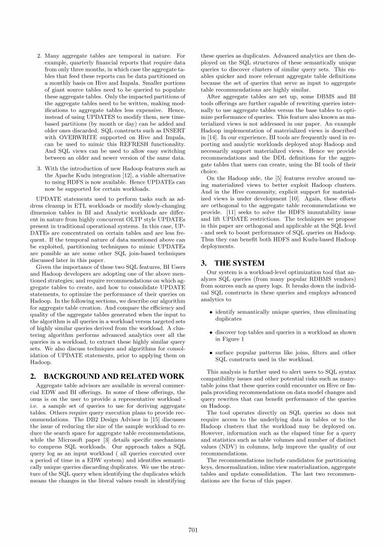
2. Many aggregate tables are temporal in nature. Forexample, quarterly financial reports that require datafrom only three months, in which case the aggregate ta-bles that feed these reports can be data partitioned ona monthly basis on Hive and Impala. Smaller portionsof giant source tables need to be queried to populatethese aggregate tables. Only the impacted partitions ofthe aggregate tables need to be written, making mod-ifications to aggregate tables less expensive. Hence,instead of using UPDATES to modify them, new time-based partitions (by month or day) can be added andolder ones discarded. SQL constructs such as INSERTwith OVERWRITE supported on Hive and Impala,can be used to mimic this REFRESH functionality.And SQL views can be used to allow easy switchingbetween an older and newer version of the same data.

3. With the introduction of new Hadoop features such asthe Apache Kudu integration [12], a viable alternativeto using HDFS is now available. Hence UPDATEs cannow be supported for certain workloads.

UPDATE statements used to perform tasks such as ad-dress cleanup in ETL workloads or modify slowly-changingdimension tables in BI and Analytic workloads are differ-ent in nature from highly concurrent OLTP style UPDATEspresent in traditional operational systems. In this case, UP-DATEs are concentrated on certain tables and are less fre-quent. If the temporal nature of data mentioned above canbe exploited, partitioning techniques to mimic UPDATEsare possible as are some other SQL join-based techniquesdiscussed later in this paper.

Given the importance of these two SQL features, BI Usersand Hadoop developers are adopting one of the above men-tioned strategies; and require recommendations on which ag-gregate tables to create, and how to consolidate UPDATEstatements, to optimize the performance of their queries onHadoop. In the following sections, we describe our algorithmfor aggregate table creation. And compare the efficiency andquality of the aggregate tables generated when the input tothe algorithm is all queries in a workload versus targeted setsof highly similar queries derived from the workload. A clus-tering algorithm performs advanced analytics over all thequeries in a workload, to extract these highly similar querysets. We also discuss techniques and algorithms for consol-idation of UPDATE statements, prior to applying them onHadoop.

2. BACKGROUND AND RELATED WORKAggregate table advisors are available in several commer-

cial EDW and BI offerings. In some of these offerings, theonus is on the user to provide a representative workload -i.e. a sample set of queries to use for deriving aggregatetables. Others require query execution plans to provide rec-ommendations. The DB2 Design Advisor in [15] discussesthe issue of reducing the size of the sample workload to re-duce the search space for aggregate table recommendations,while the Microsoft paper [3] details specific mechanismsto compress SQL workloads. Our approach takes a SQLquery log as an input workload ( all queries executed overa period of time in a EDW system) and identifies semanti-cally unique queries discarding duplicates. We use the struc-ture of the SQL query when identifying the duplicates whichmeans the changes in the literal values result in identifying

these queries as duplicates. Advanced analytics are then de-ployed on the SQL structures of these semantically uniquequeries to discover clusters of similar query sets. This en-ables quicker and more relevant aggregate table definitionsbecause the set of queries that serve as input to aggregatetable recommendations are highly similar.

After aggregate tables are set up, some DBMS and BItools offerings are further capable of rewriting queries inter-nally to use aggregate tables versus the base tables to opti-mize performance of queries. This feature also known as ma-terialized views is not addressed in our paper. An exampleHadoop implementation of materialized views is describedin [14]. In our experience, BI tools are frequently used in re-porting and analytic workloads deployed atop Hadoop andnecessarily support materialized views. Hence we providerecommendations and the DDL definitions for the aggre-gate tables that users can create, using the BI tools of theirchoice.

On the Hadoop side, the [5] features revolve around us-ing materialized views to better exploit Hadoop clusters.And in the Hive community, explicit support for material-ized views is under development [10]. Again, these effortsare orthogonal to the aggregate table recommendations weprovide. [11] seeks to solve the HDFS immutability issueand lift UPDATE restrictions. The techniques we proposein this paper are orthogonal and applicable at the SQL level- and seek to boost performance of SQL queries on Hadoop.Thus they can benefit both HDFS and Kudu-based Hadoopdeployments.

3. THE SYSTEMOur system is a workload-level optimization tool that an-

alyzes SQL queries (from many popular RDBMS vendors)from sources such as query logs. It breaks down the individ-ual SQL constructs in these queries and employs advancedanalytics to

• identify semantically unique queries, thus eliminatingduplicates

• discover top tables and queries in a workload as shownin Figure 1

• surface popular patterns like joins, filters and otherSQL constructs used in the workload.

This analysis is further used to alert users to SQL syntaxcompatibility issues and other potential risks such as many-table joins that these queries could encounter on Hive or Im-pala providing recommendations on data model changes andquery rewrites that can benefit performance of the querieson Hadoop.

The tool operates directly on SQL queries so does notrequire access to the underlying data in tables or to theHadoop clusters that the workload may be deployed on.However, information such as the elapsed time for a queryand statistics such as table volumes and number of distinctvalues (NDV) in columns, help improve the quality of ourrecommendations.

The recommendations include candidates for partitioningkeys, denormalization, inline view materialization, aggregatetables and update consolidation. The last two recommen-dations are the focus of this paper.

701

Figure 1: Workload Insights: Popular Queries andPatterns.

3.1 Aggregate Table RecommendationOur algorithm to determine aggregate tables, is similar to

[2] with a few important modifications, which are elaboratedin the subsequent sections. The first step in determining theaggregate tables is to find a set of interesting table subsets.A table-subset T is interesting if materializing one or moreviews on T has the potential to reduce the cost of the work-load significantly, i.e., above a given threshold.

In BI workloads, joins over 30 tables in a single query isnot an infrequent scenario. Such workload characteristicscould incur exponential costs while enumerating all inter-esting subsets. The enumeration of all interesting subsets of30 tables is not practical hence we need a mechanism to re-duce the overall number of interesting subsets. [1] presentsefficient algorithms to enumerate all frequent sets and [4]presents a compact way of representing all the frequent sets.However generating aggregate tables on a subset of tablesmay be more beneficial than generating it over supersets.Since enumerating all subsets can be exponential, we needto select the subsets which are still a good representation ofall the interesting subsets.

3.1.1 Merge and PruneWe address the problem of exponential subsets by con-

straining the size of the items at every step. During eachstep in subset formation, we merge some of the subsets earlyand then prune some of these subsets, without compromis-ing on the quality of the output. We use the notations men-tioned in Table 1 to describe the various concepts used inour mergeAndPrune algorithm. The detailed steps are out-lined in the algorithm 1. The algorithm takes a set of setsof tables of a given size and returns the new set with someelements merged and removed from the input.

The metric TS-Cost(T) we use is the same as that men-tioned in [2] which is the total cost of all queries in theworkload where table-subset T occurs. After we enumerateall 2-subsets ( subsets of size 2) we execute the algorithm ineach step for merging and pruning the sets early. We startwith a given element and collect the list of all candidatesthat it can be merged with. The merges are performed aslong as the merged set is within a certain threshold. Ex-perimental results indicated that a value of .85 to 0.95 is agood candidate for this threshold. We maintain a merge listand add the elements from the merge list to the prune list,

Table 1: Notations used in mergeAndPruneinput Set of sets of a given size formed by

tables in the queries.pruneSet A subset of input that holds the list

of elements that will be pruned fromthe input at the end of the iteration.

M Holds the current table set that is con-sidered for meging.

MList Holds all the sets that can be mergedwith M .

mergedSets Set of sets of tables that are formed bymerging some elements from input.

only if there is no potential for the elements to form furthercombinations of tables.

Algorithm 1 Algorithm for merging and pruning interest-ing table subsets

function mergeAndPrunefor each i ∈ input and i /∈ pruneSet do

M ← iMList← {i}for each c ∈ input do

if c ⊂M thenMList←MList ∪ ccontinue

end if. determine if the merge item is effective and not

too far off from the originalif TS-cost(M ∪ c)/TS-cost(M) >

MERGE THRESHOLD thenM ←M ∪ cMList←MList ∪ c

end ifend forfor each m ∈ MList do

. retain candidates that we should not bepruning.

if @ s| s ∈ input and s /∈ MList and s ∩ m 6= φthen

. find the candidates for pruning from inputin the later step.

pruneSet← pruneSet ∪mend if

end formergedSets← mergedSets ∪M

end forinput← input− pruneSetreturn mergedSet

end function

3.1.2 Aggregate table creation using query cluster-ing

BI reporting workloads and analytical workloads typicallygenerate queries against the same star/snowflake schema,but these queries select different sets of columns and in-voke different sets of aggregate functions i.e SUM, COUNTetc. The clustering algorithm compares the similarity ofeach clause in the SQL query (i.e. SELECT list, FROM,WHERE, GROUPBY, etc.) to pull together highly similar

702

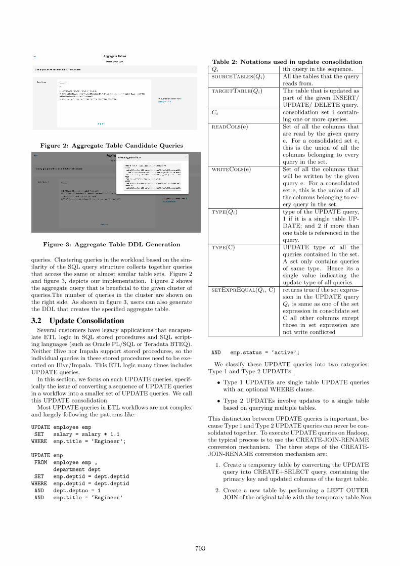
Figure 2: Aggregate Table Candidate Queries

Figure 3: Aggregate Table DDL Generation

queries. Clustering queries in the workload based on the sim-ilarity of the SQL query structure collects together queriesthat access the same or almost similar table sets. Figure 2and figure 3, depicts our implementation. Figure 2 showsthe aggregate query that is beneficial to the given cluster ofqueries.The number of queries in the cluster are shown onthe right side. As shown in figure 3, users can also generatethe DDL that creates the specified aggregate table.

3.2 Update ConsolidationSeveral customers have legacy applications that encapsu-

late ETL logic in SQL stored procedures and SQL script-ing languages (such as Oracle PL/SQL or Teradata BTEQ).Neither Hive nor Impala support stored procedures, so theindividual queries in these stored procedures need to be exe-cuted on Hive/Impala. This ETL logic many times includesUPDATE queries.

In this section, we focus on such UPDATE queries, specif-ically the issue of converting a sequence of UPDATE queriesin a workflow into a smaller set of UPDATE queries. We callthis UPDATE consolidation.

Most UPDATE queries in ETL workflows are not complexand largely following the patterns like:

UPDATE employee emp

SET salary = salary * 1.1

WHERE emp.title = ‘Engineer’;

UPDATE emp

FROM employee emp ,

department dept

SET emp.deptid = dept.deptid

WHERE emp.deptid = dept.deptid

AND dept.deptno = 1

AND emp.title = ‘Engineer’

Table 2: Notations used in update consolidationQi ith query in the sequence.sourceTables(Qi) All the tables that the query

reads from.targetTable(Qi) The table that is updated as

part of the given INSERT/UPDATE/ DELETE query.

Ci consolidation set i contain-ing one or more queries.

readCols(e) Set of all the columns thatare read by the given querye. For a consolidated set e,this is the union of all thecolumns belonging to everyquery in the set.

writeCols(e) Set of all the columns thatwill be written by the givenquery e. For a consolidatedset e, this is the union of allthe columns belonging to ev-ery query in the set.

type(Qi) type of the UPDATE query,1 if it is a single table UP-DATE; and 2 if more thanone table is referenced in thequery.

type(C) UPDATE type of all thequeries contained in the set.A set only contains queriesof same type. Hence its asingle value indicating theupdate type of all queries.

setExprEqual(Qi, C) returns true if the set expres-sion in the UPDATE queryQi is same as one of the setexpression in consolidate setC all other columns exceptthose in set expression arenot write conflicted

AND emp.status = ‘active’;

We classify these UPDATE queries into two categories:Type 1 and Type 2 UPDATEs:

• Type 1 UPDATEs are single table UPDATE querieswith an optional WHERE clause.

• Type 2 UPDATEs involve updates to a single tablebased on querying multiple tables.

This distinction between UPDATE queries is important, be-cause Type 1 and Type 2 UPDATE queries can never be con-solidated together. To execute UPDATE queries on Hadoop,the typical process is to use the CREATE-JOIN-RENAMEconversion mechanism. The three steps of the CREATE-JOIN-RENAME conversion mechanism are:

1. Create a temporary table by converting the UPDATEquery into CREATE+SELECT query, containing theprimary key and updated columns of the target table.

2. Create a new table by performing a LEFT OUTERJOIN of the original table with the temporary table.Non

703

null values in the temporary table get priority over theoriginal table.

3. Drop the original table and RENAME the newly cre-ated table to that of the original table.

If these 3 steps are needed to process each UPDATE, exe-cuting a sequence of UPDATEs can become very expensiveif the steps are repeated for each UPDATE query individu-ally. An efficient way of executing sequential UPDATEs onHadoop is to first consolidate the UPDATEs into a smallerset of queries. However, it is very important to attempt con-solidation only when we can guarantee that the end state ofthe data in the tables remains exactly the same with bothapproaches - i.e. when applying one UPDATE at a timeversus a consolidated UPDATE. Therefore, the algorithmhas to check for interleaved INSERT/UPDATE/DELETEqueries, be mindful of transactional boundaries, etc. - andonly perform consolidation when it is safe to do so.

Partitioned tables can be updated using the PARTITIONOVERWRITE functionality. If the UPDATE statement con-tains a WHERE clause on the partitioning column, then wecan convert the corresponding UPDATE query into an IN-SERT OVERWRITE query along with the required parti-tion specification. If the query is modifying a selected subsetof rows in the partition, we still have to follow the above ap-proach to compute the new rows for the partition, includingthe modified rows. In this case too, since a join is involved,it is beneficial to look at consolidation options.

Another commonly used workaround to mitigate UPDATEissues is to use database views, i.e. users access data pointedto by a normal table or in the Hadoop context a partitionedtable through a view. After UPDATEs to the table arepropagated to Hadoop by adding a new partition that con-tains updated data to the existing table or re-building theentire table that now reflects UPDATEs, the view definitionis changed to now point at the newly available data. Thisway users have access to the ‘old’ data till the point of theswitch. A similar approach, (but for the compaction usecase) is discussed here [6]. Even with this mechanism, con-solidating updates to a particular partition or table prior toapplying the updates, can minimize IO costs.

3.2.1 Update Consolidation AlgorithmWe use the notations mentioned in Table 2 to describe the

various concepts used in our UPDATE consolidation algo-rithm.

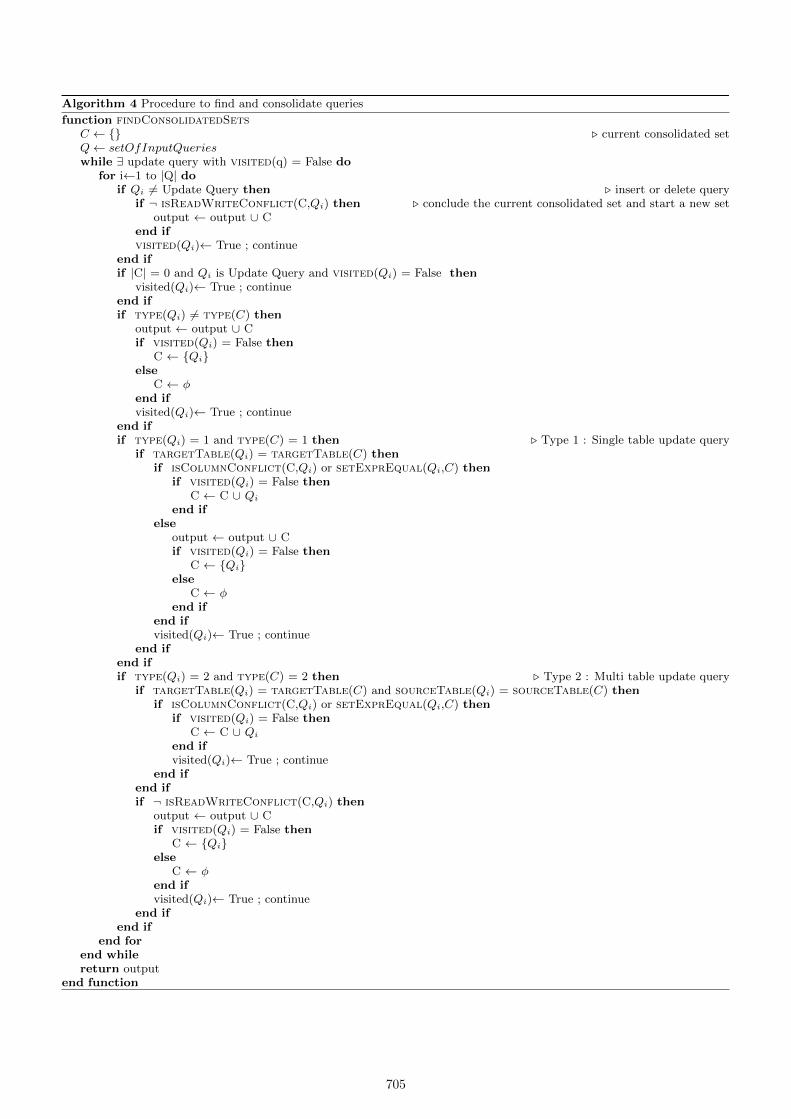
The findConsolidatedSets algorithm to consolidate UP-DATE queries is shown in Algorithm 4. The algorithm startswith an empty set and adds the first UPDATE query it findsinto the current consolidation set. Then it checks subse-quent queries to see if there are any potential conflicts withthe group in hand. Query Qi conflicts with Qj if Qj is ei-ther reading or writing a table that Qi writes to. We usethe procedure isReadWriteConfict in Algorithm 2 to de-termine the same.The UPDATE queries Qi and Qj that arereading from the same set of tables and writing to the sametable can conflict if one of the queries is writing to a col-umn, which the other query is reading from. We use theprocedure isColumnConflict in Algorithm 3 to determinethe conflict.

When we encounter a conflicting query, we stop the con-solidation process. When two UPDATE queries Qi and Qj

are in sequence with no conflicting queries in between, they

Algorithm 2 Procedure to detect conflicting queries

function isReadWriteConfict(e1,e2)if targetTable(e1) ∩ sourceTables(e2) = φ &&

targetTable(e2) ∩ sourceTables(e1) = φ && target-Table(e2) ∩ targetTable(e1) = φ then

return Trueelse

return Falseend if

end function

Algorithm 3 Procedure to detect conflicting read/writecolumnsfunction isColumnConflict(e1,e2)

if writeCols(e1) ∩ readCols(e2) = φ &&writeCols(e2) ∩ readCols(e1) = φ && writeCols(e2)∩ writeCols(e1) = φ then

return Trueelse

return Falseend if

end function

can be considered for consolidation. So we check Qi and Qj

for compatibility. Qi and Qj can be consolidated into onegroup if all the following conditions are met:

1. Qi and Qj are of the same UPDATE types - i.e. eitherboth are Type 1 or both are Type 2.

2. For Type 1 UPDATEs, the target table is the same forQi and Qj and there are no columns of Qi and Qj thatare write conflicted.

3. For Type 2 UPDATEs, the source and target tables arethe same for Qi and Qj (along with same join predi-cate) and there are no columns of Qi and Qj that arewrite conflicted.

Finally, we maintain a visited flag with each UPDATE queryso that if there are interleaved UPDATEs between totallydifferent UPDATE queries in the same stored procedure,they can be considered for consolidation.

Once we have identified a group of all consolidated sets,the conversion to the equivalent CREATE-JOIN-RENAMEqueries follows these steps. Here, without loss of generality,we assume that all WHERE predicates are in ConjunctiveNormal Form.

1. We convert each of the‘SET<col>=<colexpression>WHERE<predicates>’into‘CASE WHEN <predicates> THEN <colexpression>ELSE <col> END as <col>’

2. For queries with same SET expression and differentWHERE predicates, we create an OR clause for eachof the WHERE predicates in the CASE block.

3. We take the WHERE predicates of all the queries andcombine them using disjunction with the OR operator.If there is a common subexpression among WHEREpredicates, we promote the common subexpression out-wards.

704

Algorithm 4 Procedure to find and consolidate queries

function findConsolidatedSetsC ← {} . current consolidated setQ← setOfInputQuerieswhile ∃ update query with visited(q) = False do

for i←1 to |Q| doif Qi 6= Update Query then . insert or delete query

if ¬ isReadWriteConflict(C,Qi) then . conclude the current consolidated set and start a new setoutput ← output ∪ C

end ifvisited(Qi)← True ; continue

end ifif |C| = 0 and Qi is Update Query and visited(Qi) = False then

visited(Qi)← True ; continueend ifif type(Qi) 6= type(C) then

output ← output ∪ Cif visited(Qi) = False then

C ← {Qi}else

C ← φend ifvisited(Qi)← True ; continue

end ifif type(Qi) = 1 and type(C) = 1 then . Type 1 : Single table update query

if targetTable(Qi) = targetTable(C) thenif isColumnConflict(C,Qi) or setExprEqual(Qi,C) then

if visited(Qi) = False thenC ← C ∪ Qi

end ifelse

output ← output ∪ Cif visited(Qi) = False then

C ← {Qi}else

C ← φend if

end ifvisited(Qi)← True ; continue

end ifend ifif type(Qi) = 2 and type(C) = 2 then . Type 2 : Multi table update query

if targetTable(Qi) = targetTable(C) and sourceTable(Qi) = sourceTable(C) thenif isColumnConflict(C,Qi) or setExprEqual(Qi,C) then

if visited(Qi) = False thenC ← C ∪ Qi

end ifvisited(Qi)← True ; continue

end ifend ifif ¬ isReadWriteConflict(C,Qi) then

output ← output ∪ Cif visited(Qi) = False then

C ← {Qi}else

C ← φend ifvisited(Qi)← True ; continue

end ifend if

end forend whilereturn output

end function

705

Here are some examples of consolidations. The followingType 1 UPDATE queries that modify the table ‘lineitem’ -with or without filtering conditions:

UPDATE lineitem

SET l_receiptdate = Date_add(l_commitdate, 1)

UPDATE lineitem

SET l_shipmode = concat(l_shipmode,‘-usps’),

WHERE l_shipmode = ‘MAIL’

UPDATE lineitem

SET l_discount = 0.2

WHERE l_quantity > 20

can be consolidated and converted into a CREATE-JOIN-RENAME flow as follows:

CREATE table lineitem_tmp AS

SELECT Date_add(l_commitdate, 1) AS l_receiptdate

, CASE

WHEN l_shipmode = ‘MAIL’

THEN concat(l_shipmode,‘-usps’)

ELSE l_shipmode

END AS l_shipmode

, CASE

WHEN l_quantity > 20

THEN 0.2

ELSE l_discount 0

END AS l_discount

, l_orderkey

, l_linenumber

FROM lineitem;

CREATE TABLE lineitem_updated AS

SELECT orig.l_orderkey

, orig.l_linenumber

, Nvl(tmp.l_receiptdate, orig.l_receiptdate)

AS l_receiptdate

, Nvl(tmp.l_shipmode, orig.l_shipmode)

AS l_shipmode

, Nvl(tmp.l_discount, orig.l_discount)

AS l_discount

, l_partkey, l_suppkey, l_quantity, l_extendedprice

, l_tax, l_returnflag, l_linestatus, l_shipdate

, l_commitdate, l_shipinstruct, l_comment

FROM lineitem orig

LEFT OUTER JOIN lineitem_tmp tmp

-- lineitem table primary key

ON ( orig.l_orderkey = tmp.l_orderkey

AND orig.l_linenumber = tmp.l_linenumber )

DROP TABLE lineitem;

ALTER TABLE lineitem_updated RENAME TO lineitem;

As another example consider the following Type 2 UP-DATE queries, that modify the ‘lineitem’ table based onthe results of a join with the ‘orders’ table:

UPDATE lineitem

FROM lineitem l

, orders o

SET l.l_tax = 0.1

WHERE l.l_orderkey = o.o_orderkey

AND o.o_totalprice BETWEEN 0 AND 50000

AND o.o_orderpriority = ‘2-HIGH’

AND o.o_orderstatus = ‘F’;

UPDATE lineitem

FROM lineitem l

, orders o

SET l_shipmode = ‘AIR’

WHERE l.l_orderkey = o.o_orderkey

AND o.o_totalprice BETWEEN 50001 AND 100000

AND o.o_orderpriority = ‘2-HIGH’

AND o.o_orderstatus = ‘F’;

can be consolidated and converted into a CREATE-JOIN-RENAME flow as follows:

CREATE TABLE lineitem_tmp AS

SELECT CASE

WHEN o.o_totalprice BETWEEN 0 AND 50000

THEN 0.1 ELSE l_tax END AS l_tax

, CASE

WHEN o.o_totalprice BETWEEN 50001 AND 100000

THEN ‘AIR’ ELSE l_shipmode

END AS l_shipmode

, l_orderkey

, l_linenumber

FROM lineitem l

, orders o

WHERE l.l_orderkey = o.o_orderkey

AND o.o_totalprice BETWEEN 0 and 100000

AND o.o_orderpriority = ‘2-HIGH’

AND o.o_orderstatus = ‘F’;

CREATE TABLE lineitem_updated AS

SELECT orig.l_shipdate

, orig.l_commitdate

, orig.l_receiptdate

, orig.l_orderkey

, orig.l_partkey

, orig.l_suppkey

, orig.l_linenumber

, orig.l_extendedprice

, Nvl(tmp.l_tax, orig.l_tax) AS l_tax

, orig.l_returnflag

, orig.l_linestatus

, Nvl(tmp.l_shipmode, orig.l_shipmode) AS l_shipmode

, orig.l_shipinstruct

, orig.l_discount

, orig.l_comment

FROM lineitem orig

LEFT OUTER JOIN lineitem_tmp tmp

ON ( orig.l_orderkey = tmp.l_orderkey

AND orig.l_linenumber = tmp.l_linenumber )

DROP TABLE lineitem;

ALTER TABLE lineitem_updated RENAME TO lineitem;

We also looked at the problem of constructing a controlflow graph of the stored procedure and performed a staticanalysis on this graph. If the number of different flows aremanageably finite, we can generate a consolidation sequence

706

for each of the different flows independently thus enablingthe user to script these flows independently. However weomit all the implementation details here, as it is beyond thescope of this paper.

4. EXPERIMENTAL EVALUATIONIn this section, we evaluate the performance of the various

recommendations discussed in the previous sections usingtwo different workloads. The first workload is TPC-H atthe 100 GB scale, which we call TPCH-100. Our secondworkload belongs to a customer in the financial sector. Thiscustomer has 578 tables with 3038 number of columns. Thetable sizes vary from 500 GB to 5TB. We call this workloadCUST-1.

We have setup representative clusters to measure the per-formance of the system. This cluster has 21 nodes with 1master and 20 data nodes. The data nodes are the AWSm3.xlarge kind, with 4 core vCpu, 2.6 GHZ, 15GB of mainmemory and 2 X 40GB SSD storage. In all the experiments’time’ refers to the wall clock time as reported by the execut-ing Hive query. There are no other queries running on thesystem. For simplicity, we ignore the HDFS and other OScaches. The experiments presented should be interpreted asdirectional rather than exhaustive empirical validation.

4.1 Aggregate Table RecommendationFor aggregate table generation we ran our experiments on

the CUST-1 setup.

4.1.1 Clustering similar queriesIn our first set of experiments we evaluate the quality

of aggregate tables generated with and without clusteringsimilar queries together. We divided a workload with 6597queries into set of clusters using the clustering algorithm,thus reducing the number of queries to a group of smallerworkloads. We empirically show how this approach providesaggregate table recommendations with better run time bene-fits. The first four smaller workloads are comprised of similarqueries detected by a clustering algorithm that is run overthe 6597 queries. In the fifth workload we bundle all the6597 queries together. Figure 4 displays how the workloadsvary in size from 18 to 6597 queries.

Figure 5 and figure 6 show the results of executing theaggregate table recommendation algorithm on these 5 work-loads. As demonstrated in these results, the time taken forthe algorithm does not have a direct correlation to the inputworkload size. The algorithm converges to a solution whenit reaches a locally optimum solution. When similar queriesare clustered together the chances of the locally optimum so-lution being globally optimum are high. In our experimentswhen the algorithm is run on all the queries it convergesto a globally sub-optimum solution, recommending an ag-gregate table that benefits fewer queries - and hence has alower estimated cost saving. The estimated cost savings foreach cluster is computed as the sum of the estimated costsavings for each query in that cluster. The estimated costof each query is derived by computing the IO scans requiredfor each table and then propagating these up the join ladderto get the final estimated cost of the query. The cost savingsis the difference in estimated cost when a query runs on basetables versus the aggregated table.

Figure 4: Number of queries per workload.

Figure 5: Execution time of aggregate table algo-rithm.

Figure 6: Estimated Cost savings per workload.

707

Table 3: Merge and PruneExecution Time in milli seconds

Workload Name With mergeand prune

Without mergeand prune

Cluster 1 2.092 2.107Cluster 2 18.919 > 4hrs.Cluster 3 26.567 > 4hrs.Cluster 4 31.972 > 4hrs.Entire Workload 5.279 5.160

4.1.2 Merge and pruneIn this set of experiments we evaluate the run time of

the algorithm with and without the merge and prune en-hancement. We run the algorithm on the same workloadswe created for the earlier experiment. We terminated theexecution of the algorithm after 4 hours. In the case wherethe algorithm converges to a solution early on, removal ofmerge and prune has no effect. But in the other cases the al-gorithm without merge and prune enhancements takes morethan 4 hours to complete and so was terminated. When thealgorithm ran to completion without merge and prune, wefound no change in the definition of the output aggregatetable. The results are tabulated in Table 3.

4.2 Update ConsolidationFor update consolidation, we ran our experiments on the

TPCH-100 setup. We hand-crafted 2 stored procedures atopTPC-H data inspired from a real world customer workload.The number of consolidations we found in the stored pro-cedure are shown in Table 4. Column 2 shows the numberof queries in each stored procedure. Column 3 shows thegroups of consolidated queries represented by the index ofthe query in the stored procedure. We see that sometimethere are as many as 14 queries that are consolidated into asingle group. We also observed that with templatized codegeneration, there is a lot of scope for consolidating queries.

For comparison purposes, we take the entire stored pro-cedure and convert the queries inside it to equivalent IN-SERT/UPDATE queries. Any loops in the stored proce-dures are expanded to evaluate all updated columns - andconsider each one for consolidation. Two-way IF/ELSE con-ditions are simplified to take all the IF logic in one run, andELSE logic in the other run. N-way IF/ELSE conditionswere ignored.

From our results, we observe that on consolidating 5 queriesinto a single query, the performance impact is not 5x, for thefollowing reasons:

1. The consolidated CREATE query might have morecolumns than the individual queries, therefore the amountof data it writes will be larger.

2. If there are few or no common subexpressions, thenwe re-write the whole table or a significantly higherportion of the table.

But our performance results indicate that even with thesecaveats, UPDATE consolidation is very efficient comparedto individually mapped queries. In all our cases, we foundthat consolidating even two queries is better than individu-ally executing these queries.

Figure 7: Execution time of consolidated vs non-consolidated queries.

Figure 8: Storage requirements of update queries.

708

Table 4: Update Consolidation groupsStored procedure Number of queries Consolidation groups1 38 {6,7,9} ,{10,11} ,{12,14,16,18,20,22,24,26,28} ,{30,32,34,36}2 219 {113,119,125,131} ,{173,175,177,179,181,183,185,187,189,191,193,195,197,199}

The time taken for detecting UPDATE consolidations isless than a second; hence it was ignored in these measure-ments. We assume that the database has no triggers, allthe tables are independent and updating a table does notincur UPDATEs to tables that are not part of the query.We plot the execution time of non-consolidated queries toconsolidated queries in figure 7. The largest group with 14queries shows a performance improvement of 10x. Even fora group of 2 queries, we see a minimum performance im-provement of 80%. The baseline update performance whichis spanning few minutes is not an uncommon scenario inSQL-on-Hadoop engines.

The graph in figure 8 shows the storage ratio for consol-idated and non-consolidated queries for the size of the con-solidation group. If there are multiple groups with the samesize, we take the harmonic average of all the groups of thegiven size. The intermediate storage required for consolida-tion varies from approximately 2x to as large as 10x whencompared to the average storage requirement for individualnon-consolidated queries. However in many cases the size ofthe intermediate table is also significantly less than the orig-inal table. In the Hadoop ecosystem, storage is considered acheap resource and if performance of the UPDATE queriesis important, it is certainly worth the trade-off.

These stored procedures are part of a daily workflow thatthe customer executes, hence the time savings obtained byupdate consolidation are not only significant but also ex-tremely useful in the big data environment.

5. CONCLUSION & FUTURE WORKAs large scale new and legacy applications are deployed on

Hadoop, automated workload-level optimization strategiescan greatly help improve the performance of SQL queries.In this paper, we propose creating aggregate tables afterfirst deriving clusters of similar queries from SQL workloads,and demonstrate that in some cases execution time and ef-ficiency improvements of about 1500% can be achieved byusing clustered set of queries versus a disparate set of queriesas input to the aggregate table creation algorithm. We havealso shown empirically that a merge and prune optimiza-tion strategy helps the aggregate table creation algorithmconverge to a solution, even in cases where it could not con-verge to a solution. We also showed that 2 to 10X executiontime savings can be realized in some cases, when UPDATEqueries can be consolidated. Both these optimizations arecritical in the Hadoop environment when tables, columnsand queries are at very large scales and query response timesare of significance.

Advisors [8] [7] [15] [13] [9] rightly emphasize the needfor an integrated strategy that evaluates and recommendsaggregate table and indexing candidates, together. In theHadoop ecosystem, partitioning features are the closest log-ical equivalent to indexes. Currently, if statistical informa-tion on a table (such as table volume and column NDVs) isprovided, our tool recommends partitioning key candidatesfor a given table based on the analysis of filter and join pat-

terns most heavily used by queries on the table. We plan toextend this logic to discover partitioning keys for the aggre-gate tables, thus providing an integrated recommendationstrategy.

A further area of focus for the UPDATE consolidation op-timization is to explore opportunities to coalesce operations.For example, operations on the temporary table generatedin our algorithm can be consolidated to reduce the size ofthese tables and improve the efficiency of UPDATEs. We arealso investigating UPDATE consolidation techniques whenUPDATEs are interleaved with control-flow-logic.

Apart from the applicability of our work to adopters ofHive, Impala and Spark SQL who want to optimize theirworkloads, EDW and BI tools can also use these techniquesto improve the efficiency of their workloads.

6. ACKNOWLEDGEMENTSWe would like to thank Prithviraj Pandian for developing

the clustering algorithm used in our experiments for Ag-gregate tables. We would also like to thank our colleaguesJustin K, Parna Agarwal, Anupam Singh and Laurel Halefor their insightful review comments.

7. REFERENCES[1] R. Agrawal and R. Srikant. Fast algorithms for mining

association rules in large databases. In Proceedings ofthe 20th International Conference on Very Large DataBases, VLDB ’94, pages 487–499, San Francisco, CA,USA, 1994. Morgan Kaufmann Publishers Inc.

[2] S. Agrawal, S. Chaudhuri, and V. R. Narasayya.Automated selection of materialized views and indexesin sql databases. In Proceedings of the 26thInternational Conference on Very Large Data Bases,VLDB ’00, pages 496–505, San Francisco, CA, USA,2000. Morgan Kaufmann Publishers Inc.

[3] S. Chaudhuri, A. K. Gupta, and V. Narasayya.Compressing sql workloads. In Proceedings of the 2002ACM SIGMOD International Conference onManagement of Data, SIGMOD ’02, pages 488–499,New York, NY, USA, 2002. ACM.

[4] G. Grahne and J. Zhu. Fast algorithms for frequentitemset mining using fp-trees. IEEE Trans. on Knowl.and Data Eng., 17(10):1347–1362, Oct. 2005.

[5] J. Hyde. Discardable memory and materializedqueries, May 2014. Available athttp://hortonworks.com/blog/dmmq/.

[6] How-to: Ingest and query “fast data” with impala.Available at http://blog.cloudera.com/blog/2015/11/how-to-ingest-and-query-fast-data-with-impala-without-kudu/.

[7] Database engine tuning advisor overview. Available athttps://technet.microsoft.com/en-us/library/ms173494(v=sql.105).aspx.

[8] SQL tuning advisor in oracle SQL developer 3.0.Available at http://www.oracle.com/webfolder/

709

technetwork/tutorials/obe/db/sqldev/r30/TuningAdvisor/TuningAdvisor.htm.

[9] IBM cognos. Available at http://www.ibm.com/support/knowledgecenter/SSEP7J10.2.2/com.ibm.swg.ba.cognos.cbi.doc/welcome.html.

[10] JIRA:Add materialized views to HIVE. Available athttps://issues.apache.org/jira/browse/HIVE-10459.

[11] Apache kudu. Available at http://kudu.apache.org/.

[12] Kudu impala integration. Available at http://kudu.apache.org/docs/kudu impala integration.html.

[13] Microstrategy product documentation. Available athttps://microstrategyhelp.atlassian.net/wiki/display/MSTRDOCS/MicroStrategy+Product+Documentation.

[14] Qubole quark. Available athttp://qubole-quark.readthedocs.io/en/latest/.

[15] D. C. Zilio, J. Rao, S. Lightstone, G. Lohman,A. Storm, C. Garcia-Arellano, and S. Fadden. Db2design advisor: Integrated automatic physicaldatabase design. In Proceedings of the ThirtiethInternational Conference on Very Large Data Bases -Volume 30, VLDB ’04, pages 1087–1097. VLDBEndowment, 2004.

710