Herding, Contrarianism and Delay

in Financial Market Trading∗

Andreas Park†

University of Toronto

Daniel Sgroi‡

University of Warwick

December 20, 2011

Abstract

Herding and contrarian behaviour are often-cited features of real-world

financial markets. Theoretical models of continuous trading that study herd-

ing and contrarianism, however, usually do not allow traders to choose when

to trade or to trade more than once. We present a large-scale experiment

to explore these features within a tightly controlled laboratory environment.

Herding and contrarianism are more pronounced than in comparable studies

that do not allow traders to time their decisions. Traders with extreme infor-

mation tend to trade earliest, followed by those with information conducive

to contrarianism, while those with the theoretical potential to herd delay the

most. A sizeable fraction of trades is clustered in time.

JEL Classification: C91, D82, G14.

Keywords: Herding, Contrarianism, Endogenous-time Trading, Experiments.

∗Financial support from the ESRC (grant number RES-156-25-0023), the SSHRC, the Leverhulme

Trust and the Cambridge Endowment for Research in Finance (CERF) is gratefully acknowledged. Spe-

cial thanks go to Annie Jekova and Malena Digiuni for expert research assistance. We thank seminar

participants at the Universities of Cambridge, Toronto, Southampton, Warwick, and Zurich, and the

Midwest Economic Theory Meetings 2008 and the Northern Finance Association Meeting 2009. We

are grateful to Gustavo Bobonis, Ernst Fehr, Jordi Mondria, Jim Peck, and Xiadong Zhu for extensive

discussions, and we thank an Associate Editor and an anonymous referee for helping us improve our work.†E-mail: andreas.park@utoronto.ca‡E-mail: daniel.sgroi@warwick.ac.uk

1 Introduction

During the 2008 Financial Crisis stock markets displayed extraordinary fluctuations. From

September to mid-November 2008, there were eight days when the Dow Jones Industrial

Average changed by more than 5% in absolute terms (from close to close). Since World

War II there have been only sixteen other days where the day-to-day change exceeded

5% in absolute value. Moreover, although we perceive the time of the 2008 crisis as

a time of market decline, there were two days when the Dow rose by more than 10%.

Intra-day fluctuations were even more pronounced: on fourteen days the maximum and

minimum prices levels between two days were more than 10% apart. Such extreme price

fluctuations are possible only if there are substantial changes in behaviour (from buying to

selling or the reverse). Such behaviour and the resulting price volatility are often claimed

to be inconsistent with rationally motivated trading and informationally efficient prices.

Commentators invariably attribute dramatic swings to investors’ animal instincts, which

to most economists, is a deeply unsatisfying explanation. “Rational herding theory”,

on the other hand, provides new theoretical insights that show that seemingly erratic,

switching back-and-forth behaviour can be driven by rational, information-based motives.

Herding theory was pioneered by Welch (1992), Bikhchandani, Hirshleifer, and Welch

(1992) and Banerjee (1992) who highlight that rationality is no defence against the ran-

domness of herd behaviour.1 Put simply, a few early incorrect decisions, through a process

of rational observation and inference, can have serious ramifications for all who follow.2

A loose application of herding theory to financial market trading might suggest that early

movements by visible traders can provide a catalyst for momentum trading, induce dis-

continuous price jumps in one direction or the other, and potentially leave share prices

far from their fundamental value.

The early work on rational herding was not designed, however, for security market

trading since it did not admit prices that react to actions, whereas one key feature of

financial markets is that (efficient) market prices adjust after trades, with prices dropping

after sales and rising after buys. Furthermore, those models that do admit moving prices

restrict agents to act in a strict, exogenous sequence — they cannot decide when to

1The first published paper on the breakdown of informational learning by rational agents is Welch(1992); it is also the first application of herding theory to a financial market setting.

2Consider a setting in which agents receive an informative but noisy signal about which of two statesis better. Suppose state A is truly worse than state B. Then it is possible that the first two agents happento draw incorrect signals, and thereby opt for A. For agent 3, under a natural indifference condition, thismeans disregarding whatever signal she possesses and following the actions of the first two agents. Alllater agents find themselves in the same position as the third agent and will follow in the same mannereven though they realize that it is only the information conveyed in the first two actions that determinesbehaviour. As the direction of the herd disproportionately depends on the first movers, the ultimateoutcome is exposed to a degree of randomness that is not warranted by fundamentals.

1

trade. Finally, the latter models also restrict traders to act only once. In one of the

largest laboratory experimental studies of its type (with around 2000 trades spread over 6

treatments) we bring together all of these features: a model of financial trading with

asymmetric information across traders, the potential for rational herding and rational

contrarianism, the ability to time trades, and the ability to trade more than once.

To understand our contribution it is important to understand the history of the lit-

erature. It was first thought that when prices can adjust to actions information based

herding was either not possible or economically irrelevant. A path-breaking paper by

Avery and Zemsky (1998) introduced efficient prices to a sequential herding context, but

showed that in a simple financial market-trading setting with two values herding is not

possible because the market price always separates people with good and bad information

so that the former always buy and the latter always sell. Experimental work has confirmed

these predictions (Drehmann, Oechssler, and Roider (2005), Cipriani and Guarino (2005),

Cipriani and Guarino (2009)). More recently, however, Park and Sabourian (2011) showed

that with multiple states herding can arise and they gave conditions on information that

must be satisfied to admit rational herding; they also described conditions for rational

contrarianism.3 They showed that (economically meaningful) herding can arise by traders

who believe that extreme outcomes (big price rises or falls) are more likely than moderate

ones, and that contrarianism can arise by traders who believe that moderate outcomes

are more likely. The signals that generate these situations are, respectively, U-shaped and

hill-shaped. An experiment by (Park and Sgroi (2009)) showed that this expanded theory

has bite. We employ the information-based trading framework developed by Park and

Sabourian (2011) in our experiment.

Next, in a market-trading environment where learning from others is important, the

timing of actions may affect the possibility and extent of herding.4 First, one of the key

3Rational contrarianism is often cited as an important force for the mean-reversion of asset prices, seeChordia, Roll, and Subrahmanyam (2002).

4The seminal paper which studies investment timing with multiple agents and a single irreversibleaction, but without moving prices, is Chamley and Gale (1994) and is also explored in Gale (1996). Theirkey message is that decision makers will act very quickly in response to their information, since waitingonly makes sense when additional, new information arises. The first published experiment to considerherding in endogenous-time was Sgroi (2003), a close implementation of Chamley and Gale (1994). Thisframework was also examined experimentally in Ziegelmeyer, My, Vergnaud, and Willinger (2005). Wecomplement this line of work by explicitly considering prices that adjust after actions. There are alsotwo other related experimental papers and a theoretical paper. Bloomfield, O’Hara, and Saar (2005)study a financial market in which people can trade repeatedly throughout a trading day. The focus oftheir study is on the timing behaviour of informed traders and on their choice of limit or market ordersdepending on the passage of time. They do not employ information that could (theoretically) triggerherding or contrarianism. Ivanov, Levin, and Peck (2009) implement Levin and Peck (2008), which is amodel of fixed capital (green-field), non-financial investments, and they develop important insights intothe timing behaviour of people’s investment choices. Their setting does not, however, consider movingprices. Finally, Smith (2000) studies endogenous timing theoretically in a single trader environment and

2

features of real-world financial frenzies is the clustering of actions in time, a phenomenon

that cannot be examined when timing is not considered. Second, one can imagine that

removing yet another friction from sequential trading models may make informational

herding a non-issue. Alternatively, one can imagine that herding becomes more pro-

nounced as those with herding signals delay their actions and then rush in eventually.

Our experiment can thus shed light on the impact of the endogenous timing of actions on

herding. We identify systematic effects caused by information across treatments and par-

ticipants that are qualitatively in line with theory on the direction of trades, with marginal

effects of information that are stronger relative to exogenous timing setups. In particu-

lar we see that contrarianism is caused by hill-shaped signals, that herding is caused by

U-shaped signals, and that there is a separation of timing of trades across time by which

traders with clearly positive and negative information trade systematically before those

with U-shaped information. We also identify a new stylized fact in that traders cluster

their trading in time, thus complementing clusters in action; there is, however, no evidence

that this clustering is information- or herding-driven. In some experimental treatments,

we also explore how the ability to trade twice affects behaviour. For lack of a theory these

results are much more difficult to interpret. However, behaviour is qualitatively similar

to the single trade treatments, except that trading occurs systematically earlier.

Overview. Section 2 provides a formal definition of herding and contrarianism. Sec-

tion 3 outlines the guiding theoretical framework and develops qualitative hypotheses.

Section 4 examines the design of the experiment and lists the different treatments. Sec-

tion 5 studies the impact of information on the decision of the trade-direction. Section 6

analyzes the impact of information on the absolute and relative timing of actions (in

particular, on clusters). Section 7 studies the differential implications of the two vs. one

trade settings. Section 8 summarizes the key findings and concludes. The supplementary

appendix outlines examinations of alternative explanations, a discussion of the role of

information theory on timing, the subject instructions, and the explicit parameter values.

2 Definition of Herding and Contrarian Behavior

In the literature there are several definitions of herding. We follow Avery and Zemsky

(1998) and Park and Sabourian (2011) whose definition focuses on the social learning

(learning from others) aspect of behaviour for individual traders that is implied by the

notion of herding from the earlier literature. Specifically, this definition follows Brunner-

meier (2001)’s (Ch. 5) description of herding as a situation in which “an agent imitates

the decision of his predecessor even though his own signal might advise him to take a

offers some qualitative predictions as to which sort of information induces rapid decision making.

3

different action” and we consider the behaviour of a particular signal type by looking

at how the history of past trading can induce a trader to change behaviour and trade

against his private signal. This definition has been used in other experimental work on

social learning in financial markets (see, for instance, Cipriani and Guarino (2005) or

Drehmann, Oechssler, and Roider (2005)) and it further captures the idea of rational

momentum trading, a well-documented financial market trading phenomenon.

Definition Herding. A trader with signal S buy herds in period t at history H t if and

only if (i) he would sell at the initial history H1, (ii) he buys at history H t, and, (iii-

h) prices at H t are higher than at H1. Sell herding at history H t is defined analogously.

Contrarianism. A trader with signal S engages in buy-contrarianism in period t at his-

tory H t if and only if (i) he would sell at the initial history H1, (ii) he buys at history

H t, and, (iii-c) prices at H t are lower than at H1. Sell contrarianism at history H t is

defined analogously.

Both with buy-herding and buy-contrarianism, the trader with signal S prefers to sell

at the initial history, before observing other traders’ actions (condition (i)), but prefers

to buy after observing the history H t (condition (ii)). The key differences between buy-

herding and buy-contrarianism are conditions (iii-h) and (iii-c). The former the price

to rise at history H t so that a change of action from selling to buying at H t is with the

general movement of the prices (crowd), whereas the latter condition requires the public

expectation to have dropped so that a trader who buys at H t acts against the movement

of prices.

In our experiment each trader receives a private signal, which is one of three possible

signals (S1, S2, S3). It is important to note that herding according to our definition does

not imply that, after some history, all traders take the same action irrespective of their

private signal. Such a situation would imply an informational cascade and would be incon-

sistent with moving prices and an informationally efficient financial market. To see why,

consider the role of prices as reflecting the information contained in the traders’ actions.

If all informed types act alike then their actions would be uninformative, and as result,

prices would not move. Therefore, such uniformity of behaviour cannot explain prices

movements, which is a key feature of financial markets. Moreover, if the uniform action

involves trading, then a large imbalance of trades would accumulate without affecting

prices — contrary to common empirical findings.5

Our definition is the same as that commonly employed in the literature on infor-

mational herding, which allows comparability of our results. There are, however, other

plausible definitions of herding and contrarianism.6 Instead of defining herding and con-

5See, for instance, Chordia, Roll, and Subrahmanyam (2002).6See also Brunnermeier (2001), Chamley (2004), or Vives (2008) for related definitions of herding,

4

trarianism as switches of behaviour relative to price movements since the beginning of

trading as in (iii-h), one could define herding and contrarianism as switches relative to

the most recent price movements or actions. For instance, someone with negative infor-

mation would engage in buy herding if she buys after the price rose by x units or after

observing a sequence of y buys. The difficulty of such a classification is to find the in-

disputable criterion for the “right” number of recent actions or the right size of recent

price movements. One could also define herding and contrarianism relative to the major-

ity action. Herding would then be defined as a switch to adopting the majority action;

contrarianism would be defined as a switch to taking the opposite of the majority action.

Herding and contrarian behaviour according to such a definition would, however, occur

under similar circumstances as under our definition because, at least loosely, if the ma-

jority buys, prices rise, if the majority sells, prices fall so that, for instance, buy herding

would arise when prices rise.7

3 The Guiding Theory and Testable Predictions

Subjects face a complex decision problem, having to decide both on the timing and di-

rection of their trade. In the following, we split the description into the trade-direction

(“static”) and the trade-timing component; yet we emphasize that a full equilibrium

model requires a simultaneous description of both.

Trade Direction. The idea behind informational herding is best explained by exam-

ple. “FI”, a financial institution, has a key competitor that has just declared bankruptcy.

This may be good for FI because they may be able to attract the failed competitor’s

customers. If this situation materializes, a share of FI is worth Vh. The competitor’s

failure may also be bad since FI may have made the same mistakes as the failed bank;

a share of FI is then worth Vl < Vh. We are interested in the behaviour of a privately

informed investor, who received a (noisy) signal S and who observes several sales. Sales,

loosely, convey that the sellers had negative information. We ask if it is possible that

a trader sells when he observes many sales, even though his private (noisy) signal alone

tells him that FI is worth Vh, Pr(Vh|S) > Pr(Vl|S). Suppose that the price p ∈ (Vl, Vh)

is fixed. Then for any signal S with Pr(Vh|S) < 1 there exists a number of sales x large

including for non-financial market environments. See also Park and Sabourian (2011) for an extensivediscussion of the definition.

7One can imagine further, broader definitions that, for instance, dispense with the initial benchmarkand define herding or contrarianism only relative to the actions of recent predecessor(s). For example,one could classify a trader as engaging in herding if the trader takes the same action compared to themost recent predecessor. Yet dropping the benchmark is problematic. Suppose, for instance, that twotraders both have favourable information and buy one after the other. Arguably, they buy because oftheir information, not because everyone else or their immediate predecessor takes the same action.

5

enough such that, upon observing x sales, E[V |S, x sales] < p. In other words, even if the

private signal favours state Vh, Pr(S|Vh) > Pr(S|Vl), the trader sells because his private

information is swamped by the negative information derived from observing early sales.

There are two shortcomings to this argument. First, the price in financial markets is

not fixed. Second, traders cannot choose when to trade. The second point will play a

significant role in our experimental analysis. On the first point, if, as is a common in fi-

nancial market models, the price would be such that p = E[V |information contained in all

past trades], then we would have that for all past trading activity p ≶ E[V |S] if and only

if Pr(S|Vl) ≶ Pr(S|Vh). In other words, if the price responds to information derived from

trading, someone with favourable information would never sell, ruling out herding. Ex-

perimental evidence has confirmed this (see Drehmann, Oechssler, and Roider (2005) and

Cipriani and Guarino (2005))). Park and Sabourian (2011), however, have found that

when there are more than two possible outcomes, herding in the sense of traders trading

against their information with the majority is possible. Our experiment is guided by the

qualitative ideas of their model.

The idea in Park and Sabourian (2011) can be best explained, once again, by example.

Consider the above banking example with a third outcome, one in which FI is unaffected

by its competitor’s failure, associated with value Vm with Vl < Vm < Vh.8 Assume all

outcomes are equally likely. We are interested in the behaviour of an investor, who has

a private signal S, after different public announcements. Specifically, consider a good

public announcement G that rules out the worst state, Pr(Vl|G) = 0, and a bad public

announcement B that rules out the best state, Pr(Vh|B) = 0. Assume that the price of

the stock is equal to the expected value of the asset conditional on the public information

and that the investor buys (sells) if his expectation exceeds (is less than) the price. Note

that the price will be higher after G and lower after B, compared to the ex-ante situation

when all outcomes are equally likely.

Both G and B eliminate one state, so that, after each such announcement there are

only two states left. In two state models, an investor has a higher (lower) expectation

than the market if and only if his private information is more (less) favourable towards

the better state than towards the worse state. Thus, in the cases of G and B, E[V |G] ≶

E[V |S,G] is equivalent to Pr(S|Vm) ≶ Pr(S|Vh) and E[V |S,B] ≶ E[V |B] is equivalent to

Pr(S|Vm) ≶ Pr(S|Vl). Hence, for example, after good news G, an investor buys (sells) if

he thinks, relative to the market, that it is more (less) likely that FI will thrive than be

unaffected. It follows from the above that the investor buys after G and sells after B if and

only if Pr(S|Vh) > Pr(S|Vm) and Pr(S|Vl) > Pr(S|Vm). Such an investor, loosely, herds in

the sense that he acts like a momentum trader, buying with rising and selling with falling

8It is immaterial that the value is between Vl and Vh — any third value does the trick.

6

prices. The private information (conditional probabilities) that is both necessary and

sufficient for such behaviour has thus a U-shape. Conversely, the investor sells after G

and buys after B if and only if Pr(S|Vh) < Pr(S|Vm) and Pr(S|Vl) < Pr(S|Vm). Such

an investor, loosely, trades contrary to the general movement of prices. The private

information that is both necessary and sufficient to generate such behaviour has thus a hill-

shape. Formally, we distinguish four possible shapes of signal likelihood functions (LF):

increasing: Pr(S|Vl) < Pr(S|Vm) < Pr(S|Vh); decreasing: Pr(S|Vl) < Pr(S|Vm) < Pr(S|Vh);

U-shaped: Pr(S|Vi) > Pr(S|Vm) for i = l, h; Hill-shaped: Pr(S|Vi) < Pr(S|Vm) for i = l, h.

For the results in our paper it is also important whether the likelihood of a signal is

higher in one of the extreme states Vl or Vh relative to the other extreme state. We thus

define the bias of a signal S as Pr(S|Vh)−Pr(S|Vl). A U-shaped LF with a negative bias,

Pr(S|Vh)− Pr(S|Vl) < 0, will be labeled as an nU-shaped LF and a U-shaped LF with a

positive bias, Pr(S|Vh) − Pr(S|Vl) > 0, will be labeled as a pU-shaped LF. Similarly, we

use nHill (pHill) to describe a Hill-shaped LF with a negative (positive) bias. A signal

is called monotonic if its LF is either increasing or decreasing and non-monotonic if its

LF is hill or U-shaped. In what follows, we will refer to signals with a particular shape

of likelihood function or a trader who receives such a signal by the shape only (e.g. a

signal S with an increasing LF is referred to as an increasing signal).

Note that in the example, G and B are exogenous public announcements. In general,

however, public announcements or, more rather, public information is created endoge-

nously by the history of publicly observable trading with, loosely, G signifying a prevalence

of buying, B a prevalence of selling.

Experimental Parameters. There are three states, V ∈ {Vl, Vm, Vh} = {75, 100, 125},

all are equally likely, Pr(Vl) = Pr(Vm) = Pr(Vh). We have two types of traders: informed

traders (our laboratory subjects, who make up 75% of the trading population and who can

buy, sell or hold as they wish); and noise traders (controlled in the lab by the computer,

accounting for 25% of the trading population who buy or sell with equal probability).

While not necessary for the result, we use noise traders since we worried that subjects’

ability to count the number of trades and compare them to the number of subjects in the

room might distort the results.9 The experimental implementation of noise traders was

as follows: for a given number of possible trading decisions, noise traders were added so

that the ratio of noise to informed was roughly 1/3 (e.g. with 15 subjects, we added 5

noise traders). A coin toss for each noise trader determined whether this trader would

buy or sell. Their trade time (see below) was then a uniform draw for the possible trade

9Noise traders also add an element of realism by simulating the inclusion of traders with exogenousreasons to buy or sell, who might be of particular interest in an endogenous-time setting.

7

times (in seconds) from [0, 180].

Subjects can observe all previous prices H t. In addition, each receives one of three

signals, S1, S2, S3, which are private and conditionally i.i.d. informative. Subjects further

receive information about the signal likelihood function (hereafter: LF). Each treatment

had an increasing signal (S3), a decreasing signal (S1) and a non-monotonic signal (S2).

The rational choice for informed traders (assuming indifferent agents buy) is to buy

if their expectation of the value exceeds the price and to sell otherwise. To simplify the

experimental setting, buys and sales happen at a single price, which is set by a computer.

Subjects know that the price will adjust upwards after a buy and downwards after a sell

and they can thus infer actions from past prices (an up-tick indicates that there was a

buy, a down-tick indicates a sale).

Trade Timing. The herding theory that we allude to above is based the assumption

that traders act in an exogenous, predetermined sequence. In reality and in our exper-

iment they can trade whenever they want and we thus add to the theory by studying

this important aspect. Generally, there is no tractable model to provide us with firm

predictions about traders’ timing decisions. We can, nevertheless obtain some theoretical

guidance. Smith (2000) provides a model in which a single trader who can make a single

trade at one of two points in time (early or late). His results intuitively extend to the

case of multiple traders.10 Smith shows that a trader with a “good” or “bad” news signal

will trade early. In the Park and Sabourian (2011) setup, such signals have monotonic

LFs. Moreover, Smith also presents an example with a U-shaped signal and shows that

within his framework the recipient of such a signal would delay. In addition, we also ran

simulations (available upon request) of the trade-timing decision for the parameters used

in our experiments that indicate that for recipients of hill- and U-shaped signals there

exists a set of parameters for which delay is optimal.

The basic intuition of the timing decision is that traders generally expect prices to

move in the direction of the state which they consider most likely to occur. Traders who

think that the highest or lowest state is most likely (they have increasing/decreasing LFs)

should then act earliest because early in the round prices are (in their opinion) furthest

from their favoured state and thus profit opportunities are largest.11 Hill-shaped signals

10In Smith (2000) the trader obtains a piece of information about a public signal that will be released.After the release of this public signal, prices will adjust instantaneously to the fundamental value impliedby the signal. To see the equivalence to our setting assume that people choose a trading action (buy,sell or pass) in accordance with the optimal actions prescribed by the “static” exogenous-time theorydiscussed earlier in this section. Then their actions will affect the price and (noisily) reveal traders’information. Thus the price at the end of the trading day is, loosely, a sufficient statistic for all traders’private information. Moreover, the price is public information. Thus the price at the end of the tradingday is the same as the price in Smith (2000) after the release of the public signal. A trader’s information inour model can thus be understood as a signal about the information that will be revealed through trading.

11Formally, traders with increasing (decreasing) signals expectations of the public expectations are sub

8

are slightly different: when trading starts, prices will first be close to the hill-shaped

type’s favoured value. As prices move away from their favoured value, trading against

the movement of prices becomes most profitable. So even though their signal is quite

informative they may delay trading. At the beginning of a treatment, U-shaped types are

least sure about the direction that prices might take and they may thus delay to learn

first from the behaviour of others.

Qualitative hypotheses implied by the theory. Combing the theoretical insights,

we can develop a number of hypotheses.

Hypothesis 1 Decreasing types sell, and increasing types buy. If we observe herding then

this is most likely to be caused by U-shaped types. If we observe contrarianism, then this

is most likely caused by hill-shaped types.

In analyzing their timing behaviour we will look at the distribution of trading times and

we are interested in the relative ordering of the distributions of trading times for the

different signal types. This yields the following hypothesis.

Hypothesis 2 U-shaped types will act later than monotonic types. Hill-shaped types will

act before U-shaped types. Hill-shaped types act after the first few trades have occurred.

Multiple Trades. In much of what is to follow we are concerned with a setting where

traders can act only once. Since, in reality, people can trade multiple times, and since

there is no information-based theory that is able to describe behaviour and the influence

of information, we have also explored an experimental setting in which people can trade

twice. With two trades possible, we conjecture that types with bad and good news

should still sell and and buy respectively, and they should do so rather sooner than later.

Moreover, as prices move, traders’ information rents are reduced in expectation and thus

the greater the number of trades, the more intense is the competition for information rents.

A very straightforward assertion is thus that trades should occur earlier when people can

trade more often. We will explore the two-trade case in detail in the penultimate section.

Implementation of the market price in the experiment. One conceptual dif-

ficulty that arises in the experimental implementation is the manner in which the price

is set and updated by the central computer. For lack of a theory we used the reasonable

updating rule by which prices adjust assuming that the most recent trade was taken in

accordance with the optimal decision under exogenous-timing as implied by Park and

Sabourian (2011). For instance, in a setting with a negative U-shaped signal and absent

herding, a buy would have been assumed to come from either a noise trader or an informed

(super) martingales and they thus believe that future prices will move against them.

9

trader with an increasing signal.12 See section 4.1 for more details. Note, however, that to

detect herding and contrarian behaviour, it is not necessary that the price is set according

to any theory— the definitions speak only of increasing or decreasing prices. We are, in

fact, not testing a particular theory in all its details, but, instead, are interested in the

qualitative implications with regards to the impact of information.

We could have used other price-setting mechanisms. For instance, we could have

followed Cipriani and Guarino (2005) and used subjects as market makers; they did

this in one treatment and had two participants set prices. Our particular framework,

however, is rather complex and with human traders on both sides (market making and

active trading) we would need to worry about how traders form expectations about market

makers and vice versa. Notwithstanding this point, Cipriani and Guarino (2005) found

behaviour to be robust with respect to variations in the price-setting rules.13 Another

possible variation of the price setting mechanism is to include a transaction cost, such as

a bid-ask-spread.14

4 Experimental Design

Here we discuss the experimental design, the information provided to the subjects, and

the differences between treatments. The supplementary appendix contains a time-line

(Appendix C), a full set of instructions and the materials given to subjects (Appendices

D-F), and a description of the custom software used in this experiment (Appendix G).

4.1 Overview

Each group of traders was made up of 13-25 experimental subjects. At the beginning of

the session, subjects were given information about the trading system, the kind of signals

that they may receive, and the functioning of the market. Subjects were told that they

would not interact directly with each other but rather that the trades were with a central

computer. Subjects were explicitly told that the price would be increased by the central

computer following a buy decision, and would be decreased following a sell decision and

that they would have access to the full price history generated by the central computer

(provided by the experimental software in the form of a price-chart).

12This rule does, however, become problematic with multiple trades because two trades by the sameperson will be counted as two separate pieces of information.

13We are grateful to an anonymous referee for making this point.14An earlier working paper version of Drehmann, Oechssler, and Roider (2005), dated April 2003,

evaluates the impact of transaction costs. They find that transaction costs make “not trading” optimalfor some prices (when at such prices the gain from trade is lower than the cost) and so trading breaksdown. Since this effect is well-understood we ignored transactions costs and instead focused on theinformation structure as the key differentiating factor between treatments.

10

Prior to running sessions, for each of the six rounds, we had a random draw for the

true value (and thus in all sessions, subjects received signals according to the same LF).

For each round, each subject received a private signal, either S1, S2, or S3, where signals

were drawn using the LFs for the underlying treatment given the true value draw (e.g., the

practice round was based on a treatment with an nU-shaped LF and true value V = 100).15

Prior to the start of each treatment, subjects were provided with an information sheet

detailing the signal likelihood function (i.e. information about all possible signals) and

the posteriors that each signal would imply. The information on the sheet was common

knowledge to all subjects. The subjects were not told anything about the implications of

U-shaped, hill-shaped or monotonic LFs.

All of the experimental subjects took part in all of the rounds in each session (the

practice round plus all 6 incentivized rounds) and they were all made aware of this fact.

The practice round was special in two senses. Firstly, it was not incentivized and this was

stressed, so subjects could use it to get used to the software, and as such it is not included

in the results. Secondly, they were allowed to ask questions pertaining to understanding,

after the practice round. Information for the round was presented in the same format as

for the incentivized rounds.

The subjects received financial incentives to ensure that they took the tasks seriously

as is standard practice within experimental economics (excluding the unpaid practice

round). First, subjects were provided with a show-up fee of £5 (in UK currency, or

equivalent in Canadian currency) and this was known to the subjects. Second, it was

explained to the subjects that their bonus payment would depend precisely upon the

actual value of each share and the price at which they sold or bought the share (both

denominated in virtual currency units or VCU) and examples were given to make this

clear, for example:

“If you buy a share at a price of 90 vcu, and after the event takes place the price of

the share is updated to 125 vcu. You have therefore made 35 vcu of virtual profits on

your trade. If you instead sold at 90 vcu you would have lost 35 vcu. If you did nothing

you would make a profit of 25 vcu since your share was originally worth 100 vcu and is

worth 125 vcu after the event is realized.”

It was further explained to the subjects that the central computer would maintain a

running total of their winnings in VCU after each round and this would be converted to

real currency at the end of the session and that this could reach a possible maximum of

£25 (in UK currency, or equivalent in Canadian currency). Subjects made an average

of £7.70 in total bonus payments (across all 6 rounds) or £12.70 in total including their

show-up fee. The subjects were informed that the rounds would last 3 minutes and that

15Figures 2-4 in the supplementary appendix describe the signal LFs.

11

they would receive announcements about the remaining time after 2:30 minutes, and 2:50

minutes. Each round was followed by a cool-off period of about 1-2 minutes and then

subjects were given information for the next round. They had about 2-3 minutes to digest

this new information. They were told in advance (as early as at the recruitment stage)

that each session would last approximately 1 hour.

The existence and proportion of noise traders (roughly 25% of trades, see Section 3)

was made known to the subjects in advance. Subjects were also aware that noise traders

randomized 50:50 between buying and selling and that they traded at random times.

We considered two classes of treatments: in the first, subjects were allowed to trade

once, in the second they could trade twice. The software allowed subjects to trade at

most this specific number of times. The sequence of transactions produced a history of

actions and prices, Ht with t ∈ [0, 180], that recorded the timing (in seconds), price,

and direction of each transaction. Subjects were shown the history in the form of a

continuously updating price chart during each treatment, and they were also given the

current price, Pt, where P0 = 100.

Subjects were told that they had three possible actions a = {sell, pass, buy} one

(or two) of which they could undertake during the 3 minutes of trading time.16 For the

treatments in which two trades were allowed, subjects were additionally informed that

they could trade twice, so they could “buy and buy”, “sell and sell”, “sell and buy”, etc.

as and when they wished during the three minute period. They were instructed that

pressing the “pass”-button would count as one of the actions that they were allowed. It

was stressed to the subjects that their virtual profits per treatment were generated based

on the difference between the price at which they traded, Pt, and the true value of the

share, V . It was emphasized that the price at the end of the trading round would not be

relevant for their payoffs.

The subjects themselves were recruited from the Universities of Toronto, Cambridge

and Warwick. No one was allowed to take part twice. We ran 13 sessions in all: 3 at the

University of Cambridge (13 subjects each), 6 at the University of Warwick (18, 19, 22, 22,

22, and 25 subjects) and 4 at the University of Toronto (17, 18, 13, and 13 subjects). We

collected demographic data only for the Warwick sessions: of the subjects there, around

49% were female, around 73% were studying (or had already taken) degrees in Economics,

Finance, Business, Statistics, Management or Mathematics. 53% claimed to have some

prior experience with financial markets, and 23% claimed to own or have owned shares

at some point.17

16The “passing” decision is a relict of a setting with exogenous timing. Instead of pressing a holdbutton, traders could also just not trade. We have not analyzed this decision separately.

17Appendix E details the questions asked in the questionnaire. When asked what motivated theirdecisions (across different rounds) 44% of subjects mentioned a combination of prices and signals, 31%

12

4.2 Treatments

In our setup, each round of play corresponds to a unique treatment.18 In Treatment 1,2,

and 3, subjects were allowed to trade at most once, in treatments 4,5, and 6 subjects

were allowed to trade at most twice. Each treatment included signals with an increasing,

a decreasing and a non-monotonic LF, where Treatment 1 and 6 had a signal with an

nU-shaped LF, Treatment 2 and 4 a signal with a nHill-shaped LF, Treatment 3 and 5

had a signal with a pU-shaped LF. The underlying parameters and signal LFs are listed

in the supplementary appendix together with the instructions given to subjects.

The specific signal structures by rounds were as follows:19

• Round 1: negative U-shaped LF making buy herding possible;

• Round 2: negative hill-shaped LF making buy-contrarianism possible;

• Round 3: positive U-shaped LF making sell-herding possible;

• Round 4: as Round 2 but with two trades;

• Round 5: as Round 3 but with two trades;

• Round 6: as Round 1 but with two trades.

The same order of treatments was maintained across all sessions.20

4.3 Behavioral, non-rational predictions for the static decision

To complete the analysis, we considered the possible impact of risk aversion and loss

aversion on decision making, and various behavioural alternatives to Bayesian updating.

First, we considered a model in which subjects do not update their beliefs as prices change

but act solely on the basis of their prior expectation. Second, we considered one setting

in which subjects update their beliefs on the basis of changing prices at a slower rate than

they should and one setting in which people overweigh their own private information.

only price, 18% only signal and the remaining 7% had other motivations. 38% thought that in generalthe current price was more important than the signal, 36% thought the signal was more important thanthe current price and the remaining 26% felt they were of similar value. Roughly 24% claimed to havecarried out numerical calculations.

18So treatment 1 occurred in round 1, treatment 2 in round 2, etc.19The practice round was a one-trade treatment with a negative U-shaped signal structure.20Since each round was only played once, and since prior to any rounds a practice round was undertaken

we believe that learning between rounds would be minimal. There was no econometric evidence of learningbetween rounds. For instance, there was no discernible trend in behavior. In untabulated regressions wealso clustered standard errors by rounds and double-clustered standard errors by rounds and subjectsand found that the results were unchanged.

13

Finally, we developed error correction models in which subjects account for errors made

by their peers and react rationally to these errors; these models are in the spirit of level-

k beliefs (see Costa-Gomes, Crawford, and Broseta (2001)) and the Quantal Response

Equilibrium (see McKelvey and Palfrey (1995) and McKelvey and Palfrey (1998)).

The full details of the alternative specifications and tests can be found in Section A

of the supplementary appendix.

5 Signals and Herding or Contrarianism

5.1 Observations from Summary Statistics

The total number of trades made by experimental participants was 1991 spread over all

6 treatments; broken up by trader type we have 623 (S1), 786 (S2) and 584 (S3). For

treatments 1 to 3 we had 683 trades (197 S1, 276 S2 and 210 S3), for treatments 4-6 there

were 1308 (425 S1, 510 S2 and 373 S3) trades. Overall, we observe that the monotonic

types, S1 and S3, always sell/buy in 85% of all their trades.

One of the main questions that we want to answer is whether U-shaped signal types

switch from selling to buying if prices rise and whether they switch from buying to selling if

prices fall, i.e. that they herd in the sense of following the “majority” action. The “static”

theory, applicable under exogenous sequencing, of Park and Sabourian (2011) suggests

that only U-shaped types would herd. Yet the definition of herding and contrarianism

does not rule out that other types herd or act as contrarians. Table 1 gives the raw

numbers on trading behaviour, split by signal types.

Finding 1 (Hypothesis 1, summary statistics) U-shaped types herd in 26% of pos-

sible cases, hill, increasing and decreasing types herd in 4%, 10% and 21% of all cases.

Contrarianism arises more frequently, most stemming from hill-shaped types (67%). De-

creasing, increasing, and U-shaped types act as contrarians in 31%, 19% and 37% of all

possible cases.

The fraction of herding actions is larger than that observed in Drehmann, Oechssler, and

Roider (2005) or Cipriani and Guarino (2005); these papers also found persistent evidence

of contrarianism, albeit to a smaller extent.

5.2 Regression Analysis of the Trading Direction Decision

We ask the following questions:

(1) Given that someone has a herding (U-shaped) signal, is this person more likely to

herd than someone who does not have the herding signal?

14

(2) Given that someone has a contrarian (hill-shaped) signal, is this person more likely

to act as a contrarian than someone who does not have the contrarian signal?

The random assignment of signals to traders allows us to interpret mean differences

in signal-specific effects as the average causal effect of the signal. Formally, we estimate

the following equations to test whether a type of signal is a significant cause for herding

or contrarian behaviour respectively:

herdi = α + βu-shapei + fixedi + ǫi, contrai = α + βhill-shapei + fixedi + ǫi (1)

where the dependent variables herdi and contrai are dummies that apply the Herd-

ing/Contrarianism Definition in the sense that they are set equal to 1 if the current

trade by individual i is a herding and contrarian trade respectively and 0 otherwise, α is a

constant, and u-shapei and hill-shapei are signal dummies that are set equal to 1 if the in-

dividual who performs the current trade received a U-shaped (for the herding estimation)

or hill-shaped (for the contrarian estimation) signal. Parameter fixedi is an individual

fixed effect that controls for specific traders who persistently err.21 Given the random

assignment of signals, we can assume that E[u-shapei · ǫi] = 0 and E[hill-shapei · ǫi] = 0,

which are the main identifying assumptions. In our estimations we cluster standard er-

rors at the trader (individual) level to correct for unobserved components at the trader

level. We run the regressions restricted to the cases for which herding and contrarianism

respectively are possible.

In each scenario we estimated the model by logit without fixed effects and by a linear

model with fixed effects. For logit estimations, we report the marginal effects at the mean.

Further, we report the results across all six treatments; in the penultimate section, we

expand the analysis to check if the number of trades affects the estimates (it does not).

For the herding specification, β represents the impact of the signal on the average

individual’s choice of whether or not to herd. If it is positive and significant, then a

U-shaped signal increases the probability of herding relative to all other signals. The first

two columns in Table 2 summarize the result from our regression. Overall, obtaining a U-

shaped signal increases the probability of herding by about 12% relative to any other signal

and it is significant at all conventional levels. Parameter estimates are large unaffected by

fixed effects. Overall the regression confirms the hypothesis that recipients of U-shaped

herding-type signals are generally more likely to herd.

For the contrarianism specification, coefficient β represents the impact of the signal on

the average individual’s choice of whether or not to act as a contrarian. If it is positive and

significant then the hill-shaped signal increases the probability of contrarianism relative

21In unreported regressions we also controlled for treatment, session and treatment-session fixed effectsas well. The results remain unaffected.

15

to all other signals. The first two columns in Table 3 summarize the results from our

regression. Receiving the hill-shaped signal increases the chance of acting as a contrarian

by 36-40% relative to any other kind of signal. All coefficients are significant at all

conventional levels. Overall we confirm that the hill-shaped signal is the significant source

of contrarianism relative to all other signals.

Finding 2 (Hypothesis 1, regression analysis) The U-shaped and hill-shaped signals

are the significant sources for herding and contrarianism respectively.

Our findings here are noteworthy for two reasons. First, (irrational) contrarianism

has been observed in other experiments before (e.g. Drehmann, Oechssler, and Roider

(2005), Cipriani and Guarino (2005), Alevy, Haigh, and List (2007)). Thus arguably,

people exhibit a general tendency to act against the crowd. Here we show that despite

this tendency, contrarianism is still most likely caused by recipients of signals that admit

contrarianism theoretically: so observed contrarianism is not necessarily irrational, but

may be the result of sensible, information-based considerations. Second, the marginal

effect of a U-shaped signal on the probability of herding is stronger than that in our

exogenous timing companion paper, Park and Sgroi (2009). Combined with the fact that

U-shaped types do not herd as much as they should theoretically, this implies that due to

the timing of actions non-U-shaped types herd proportionately less and U-shaped types

herd proportionally more than with exogenous timing: so the importance of signals that

are conducive to herding increases with the potential to delay.

6 Signals and the Timing of Actions

6.1 Absolute Timing

The key question to address is whether there are systematic differences in the timing

behaviour for the various signal types and treatment settings. To identify such differences,

we compare the cumulative distributions of the trade-times for different categories of

types. The strongest result that one can hope for in this context is that one cumulative

distribution function (henceforth, cdf) of trade-times stochastically dominates another:

distribution F first order stochastically dominates distribution G if G is larger than F for

all entry times. If we indeed observe that F first order stochastically dominates G, then

we can say that the entry times under F are systematically later than under G.

We computed the cdfs for a large variety of subsamples, such as treatments 1-3, 4-5,

4-5 (first trades), and so on. The timing pattern for increasing and decreasing signals

showed no differences, neither did positive and negative U-shaped signals. In presenting

16

the results, we thus combine increasing and decreasing signals as “monotonic” signals,

and we combine positive and negative U-shaped signals as “U-shaped signals”. Moreover,

we also aggregate trading times for the respective types across all treatments. Figure 1

provides plots of the relevant differences of cdfs.22 We find the following.

Finding 3 (Hypothesis 2) U-shaped types trade later than monotonic types.

Consequently, our findings comply with Smith (2000)’s prediction that people with good-

news (increasing) or bad-news (decreasing) signals trade early, and that people who receive

mixed information delay. The bottom right panel displays the relation of the hill-shaped

types’ timing to the U-shaped types.

Finding 4 (Hypothesis 2) On almost the entire domain (apart from the first few sec-

onds) the hill-shaped type trades systematically earlier than the U-shaped types.

To consider Hypothesis 2, one can compare the top right and bottom right panels. As

can be seen, for the first few seconds, more trades stem from non-hill-shaped types. Yet

after these first few trades, the hill-shaped types trade strongly (this follows as their cdf

rises strongly relative to the other cdfs).

Finding 5 (Hypothesis 2) The trades by hill-shaped types are concentrated after the

first few transactions have occurred.

In the supplementary appendix we further examine if pure information theory can ex-

plain the timing of decisions. As is common in the literature on information theory we use

the entropy of posteriors to measure the informativeness of a signal. We observe, however,

that information theory does not seem sufficient to explain the timing of decisions.

6.2 Relative Timing: Clustering

The word “herding” semantically suggests not only that people take the same action,

but also that people act at almost the same time. Definitions of herding (such as ours)

and models of herding do not capture the timing decision and, since the models typically

force actions to be taken in a strict exogenous sequence, thus have no built-in simul-

taneity. During the experiments, however, we did observe that traders often acted at

almost the same time. This behaviour, which has not been identified before in laboratory

experiments, is in the spirit of the mass behaviour that one may associate with herding.

22Tests of stochastic dominance have low power. The plots of cdfs that we show here, however, painta very clear picture in that for almost the entire domain we observe a clear ordering of the distributionsof trading times.

17

We categorize this trading at almost the same time as “stimulus-response” driven

trading in the sense that one trade triggers others in short succession. We thus define

a trade to be triggering if it happens 5 or 10 seconds after its predecessor (this time

separation avoids spurious proximities of trades) and at least 5 seconds after the first

trade in the round. We then define a cluster as a situation where at least 2 more trades

occur within 3 seconds of the triggering trade.23 Table 4 provides summary statistics

and indicates that there are a sizeable number of clusters. For instance, those with 5-

second delays occur, on average twice in each treatment, those with 10 seconds about

once. Furthermore, a large fraction of trades is involved in a cluster (between 21% for

5-second delays and 10% for 10-second delays), which is remarkable because more than

25% of trades occur so early that are excluded by design.

There are several questions to ask. First, why do people trade in a cluster? Second,

are clustered trades herding or contrarian trades in the sense of trade-direction? Third,

do signals plays a role in the decision to cluster?

As for the first question, the simplest explanation for why clusters arise is that some

traders play a (delay-) strategy which includes a conditioning of the form “wait until

the next trade and then act”. If traders play such a strategy then, naturally, one trade

may trigger another or several others,24 and it is important to understand to what extent

information affects this type of behaviour.

A more complex explanation as to why it may pay to trade in a cluster is as follows.

One feature of our experimental setup is that prices are set assuming that each trade is

performed by a noise trader with constant probability. Although it would be difficult to

argue that a trade that triggers a cluster is more or less likely to be informed, a trade

that follows another in close succession may well be more likely by an informed trader.

In this case, the price adjustment following this trade is too small because the price

adjustment accounts for the possibility of noise. Consequently, one may argue that it

may be profitable to be the third person in a cluster and to trade in the same direction

as the second.25 We try to capture this idea in a regression where we control for trades

23The timing numbers used in our definition of a cluster were based on giving traders enough timeto observe a change in price on their screens, infer the direction of trade required to produce this pricechange, make a trading decisions in response and then initiate it: 5-10 second seems enough time to dothis for the first trade to reply to the triggering trade, while a further 3 seconds seems enough to capturetrades in the same cluster, but not so long as to admit trades generated in reply to a new triggering trade.We performed the analysis with several variations of these numbers and found behaviour to be similar.

24Argenziano and Schmidt-Dengler (2010) show that in an N-player pre-emption game clusters canarise naturally as part of an equilibrium strategy. Their model is, however, a fixed-investment frameworkwith an exogenous delay benefit (which we do not have) and without moving prices.

25On theoretical explanation for clustering is given by Admati and Pfleiderer (1988) who show thatclustering can be rational as informed traders trade more aggressively when they believe that there aremore uninformed traders around. Their idea is, however, not directly applicable to our model, becausewe do not have the simultaneous order submission that is the basis of Admati and Pfleiderer (1988).

18

that are in the same direction as their predecessor.

To understand all the above questions, we ran the following regression:

clusteri = β0 + β1herdi + β2contrai + β3u-shapei + β4increasingi

+β5decreasingi + β5round tripi + β6same as beforei + fixedi + ǫi, (2)

where herdi, contrai, u-shapei, increasingi, and decreasingi are the usual herding, contrari-

anism and signal dummies, clusteri is a dummy that is 1 when the current trade is in a

cluster and 0 otherwise, round tripi is a dummy that is 1 if the trader who made this trade

makes his other trade in the opposite direction (buy-sell or sell-buy), and same as beforei

is a dummy that is 1 if the current trade is in the same direction as the trade just before

it and zero otherwise. These covariates are, in essence, all effects that could play a role

in our analysis. We ran these regressions, as before, for a linear probability model with

and as a logit model without fixed effects. Moreover, we classified trade clusters in two

ways: the first included the triggering trade as part of the cluster, the second omits the

triggering trade. Overall, we find the following:

Finding 6 With the exception of the U-shaped signal for 5-second quiet periods before

trades, none of the covariates in (2) is persistently statistically significant.

This finding is, of course, a negative result: although one can argue that clustering may be

caused by a delay strategy (“act after the next trade”), one may have suspected that, for

instance, signals should have played a role, i.e. that some types of signals are more likely

to delay and thus act in clusters than others. Yet we found essentially no persistence

or explanation for traders’ behaviour, except that the occurrence of clusters themselves

and we are thus left with the stylized fact that subjects tend to trade in unison, a finding

which represents an important area for future research.

7 The Second Trade

7.1 Herding and Contrarian Estimates with One vs. Two Trades

In half of our treatments, subjects have the option to trade twice. One natural question

is whether this option affects the impact that signal have on the chance of engaging in

herd behaviour. To answer this question, we ran the following regression:

herdi = α + β1u-shapei × 1-tradei + β2u-shapei × 2-tradei + β31-tradei + ǫi, (3)

contrai = α + β1hill-shapei × 1-tradei + β2hill-shapei × 2-tradei + β31-tradei + ǫi, (4)

19

where herdi, contrai, u-shapei, and hilli are the herding, contrarianism, U- shape and hill-

shape indicators from (1), 1-tradei and 2-tradei are 1 if the trade was made in a one- and

two-trade treatments respectively. Parameters β1 and β2 then reveal the marginal effect

of a U- and hill-shaped signal respectively in the one- and two-trade treatments. The

third and fourth columns in Tables 2 and 3 display the estimates. At the bottom of the

table we present the results of an F-Test for equality of the coefficient estimates β̂1 and β̂2.

Columns five and six perform the same analysis, where we further differentiate between

the first and second trade in the two trade treatments.

Finding 7 The coefficient estimates for the impact of signals on the probability of herding

and contrarianism are robust to the number of trades in that we cannot reject the hypothesis

that they coincide. Signals do not, however, have the same impact on the second trade

being herding or contrarian.

7.2 The Impact of Round-Trip Trades

The fact that signals have a reduced effect on the second trade is noteworthy. One

possibility is that subjects followed an altogether different strategy when making their

second trade. Namely, with two trades, traders have the opportunity to make so-called

“round-trip” or “return” trades by selling first and then buying later or vice versa. This

way, they can realize a trading profit in the process.

Table 6 provides summary statistics for the second trade in general, and shows that

about 23% of second trades are part of a round trip transaction. About 76% of the return

trades yielded a trading profit which suggests that return-trades were performed on the

basis of “buy low, sell high” (or “sell high, buy low”). Furthermore, most of round-trip

trades are performed by the hill- and U-shaped types.

All this indicates, that traders may well have a particular, possibly non-information-

based strategy, in their trading and that this may affect our estimate of herding and

contrarianism. A trader who merely aims to buy low and sell high may thus act for

reasons that have little to do with his information. Yet in our analysis thus far, this

trader’s actions may be classified as herding or contrarian and we would thus obtain

spurious estimates.

We thus analyze to what extent our estimates in Tables 2 and 3 change when we take

account of this possible misclassification. We ask the following question: what is the

probability that a first/second trade is a herding trade conditional on the trade being a

return trade (when herding is possible) relative to the case where it is not a return trade?

20

To answer this question, we ran the following regressions

herdi = α + β1u-shapei + β2return tradei + β3u-shapei × return tradei + ǫi, (5)

contrai = α + β1hill-shapei + β2return tradei + β3hill-shapei × return tradei + ǫi. (6)

The dependent variables herdi and contrai are the herding and contrarian dummies from

the equations in (1), u-shapei and hill-shapei are the signal dummies, α is a constant,

return tradei is a dummy for the incidence of a return trade (both the first and second

transaction of a return trade have value 1), and u-shapei × return tradei and hill-shapei ×

return tradei are products of the two dummies.

For each case we estimated the model by logit, restricted to incidences where herd-

ing and contrarianism respectively can occur, and we report the marginal effects. The

coefficient β1 allows us to estimate the marginal effect among non-return traders and the

coefficient β3 allows us to estimate the differential marginal effect among return traders,

so that β1 + β3 allows us to determine the effect of a signal among return traders.

Table 7 summarizes our findings and indicates that our herding estimates from Sec-

tion 5 are biased downwards by round-trip trades (the coefficients on the product term are

negative and significant) and that our contrarian estimates are unaffected. This is good

news for our analysis as it indicates that, if anything, the effect of a herding signal as a

source for herd behaviour is underestimated by the possibility of round trip transactions.

Finding 8 (Impact of Return Trades on Estimates for Hypothesis 1) The esti-

mates underlying Finding 2 for herding become stronger and those for contrarianism re-

main unaffected when we correct for round trip transactions.

7.3 The Timing of Actions with One vs. Two Trades

Our final question concerns the timing of trades of one-trade relative to two-trade treat-

ments. Since informed traders compete to exploit their private information, more trades

imply higher competition for information rents which, under our price-setting regime,

should speed up trading. The panels in Figure 2 plot the differences of cdfs of timing,

where we aggregated all trades in treatments 1-3 and 4-6 as well as first and second trades

in treatments 4-6.

Finding 9 Allowing people to trade twice accelerates their trade-times: (1) The first trade

in treatments 4-6 occurs earlier than the single transaction in treatments 1-3. (2) The

single trade in treatments 1-3 occurs earlier than the second trade in treatments 4-6.

(3) All trades together in treatment 4-6 occur earlier than in treatments 1-3.

21

To assess this finding, suppose subjects’ timing strategies for their trade time T in the

single trade treatment could be described by some density f on [0, 180] and consider the

following two timing strategies as benchmarks.26 In the first, traders choose the times for

their two trades τi, τj according to some joint density f(τi) · f(τj) over [0, 180]. In the

second, traders choose the time t1 of their first trade according to f(t1) and then choose

the time t2 for their second trade on [t1, 180] according to f(t2|t2 ≥ t1). Applied to our

trading setup, the first specification loosely implies that the subjects apply their single-

trade timing strategy as independent draws to the two trades; the second specification

implies that traders apply the same strategy for the single and first trade and then apply

the same strategy of their first trade to their second trade, conditional on the execution of

the first trade. Intuitively, the first specification would then imply that the distribution

of trade times is such that the first trade for the two-trade specification occurs before

the single trade, but that the distributional order for all trades is unclear.27 The second

specification would imply that the distribution of trade times is such that trades for the

two-trade specification occur before the single trade, but that there should be no order

when comparing the first trade for the two-trade specification with the single trade.

Neither of these benchmarks implies that the first trade of the two-trade specification

and all trades taken together from the two-trade specification occur earlier than the

single trade from the one-trade specification. Our finding thus indicates that there is an

accelerating effect when traders can trade more often that is distinct from the pattern

that would emerge from the two benchmarks that we discuss above.

8 Conclusion

Herding has long been suspected to play a role in financial market booms and busts. Re-

cent theoretical work shows that informational herding is possible if the signal likelihood

function for traders has a specific shape. Other work shows that when timing is endoge-

nous to the decision, traders with good or bad news should trade earlier than those with

less informative signals. Giving traders a choice of when to act is not only natural, but

26The idea is that players play a symmetric mixed strategy with full support on the available timeinterval; implementing this strategy, the probability that a trader has played up to time t can be describedby a distribution, and, for simplicity, we assume here that it has density f .

27We are grateful to an Associate Editor for making this point. In support of this argument we ranthe following simulation which assumes that traders play a uniform timing strategy. We first generated1 million uniformly distributed trades on the [0,180] interval. These observations are used as the singletrade times. We then generated another 2 million observations which are interpreted as trade-times forthe two-trade settings. We randomly form 1 million pairs with the smaller element being the first trade,and the larger the second trade. For these trades, we carried out the same distribution computations asfor our sample and observed the described pattern. The simulations invoke the Mersenne-Twister method(designed to generate a high level of pseudo-randomness and to avoid serial correlation).

22

there are also important insights that can be gleaned from such an analysis.

It is not clear ex ante, how the decision to time one’s trades should affect herding

and contrarianism. One possibility is that when herding-prone types delay their actions

systematically, herd behaviour can become more pronounced and significant compared

to exogenous timing settings. On the other hand, research by Drehmann, Oechssler,

and Roider (2005) and Cipriani and Guarino (2005) has revealed that people have a

general tendency to act as contrarians. Another possibility thus is that by removing the

artificial friction of exogenous timing, herding disappears. Our work directly addresses

this open question.

Having collected almost 2000 trades, we found that subjects’ decisions were generally

in line with the qualitative predictions of the information theory learning theory when

that theory admits rational herding and contrarianism. For example, types theoretically

prone to herd or be contrarian are the significant and important source of this kind of

behaviour when it does arise. Furthermore, types with extreme information about an

asset (both good or bad) trade systematically earliest, and those with signals conducive

to contrarianism trade earlier than those with information conducive to herding. We thus

find strong evidence for the impact of the type of information both with respect to the

direction and the timing of trades.

We can break our findings down further into four key messages. First, we find addi-

tional and qualitatively novel support for information-based motives for herding theory in

the laboratory. Second, adding endogenous-timing leaves the key predictions of sequential

herding theory unchanged as far as the direction of trade is concerned. Therefore, our

results suggest that earlier work which forces subjects to act in a strict sequence remains

valid even though the timing assumptions impose an artificial friction. Third, we com-

bine two literatures by linking information-based trade directions and timing and show

that signals that push subjects towards herd or contrarian behaviour also push them to-

wards delay, relative to the signals that guide subjects towards clear buy or sell decisions.

This point is a potentially important avenue for future research as the combination of

herding/contrarianism in decision-making and clustering in time can work together to

potentially exacerbate/counter prices movements which drift away from fundamentals.

Finally, we also identify a new experimental stylized fact in that traders tend to cluster

their actions in time. This final key finding represents a potentially important avenue for

future research.

23

References

Admati, A., and P. Pfleiderer (1988): “A Theory of Intraday Patterns: Volume and

Price Variability,” Review of Financial Studies, 1, 3–40.

Alevy, J. E., M. S. Haigh, and J. A. List (2007): “Information Cascades: Evidence

from a Field Experiment with Financial Market Professionals,” Journal of Finance,

LXII(1), 151–180.

Argenziano, R., and P. Schmidt-Dengler (2010): “Clustering in N-Player Preemp-

tion Games,” Working paper, University of Essex.

Avery, C., and P. Zemsky (1998): “Multi-Dimensional Uncertainty and Herd Behavior

in Financial Markets,” American Economic Review, 88, 724–748.

Banerjee, A. V. (1992): “A Simple Model of Herd Behavior,” Quarterly Journal of

Economics, 107, 797–817.

Bikhchandani, S., D. Hirshleifer, and I. Welch (1992): “Theory of Fads, Fash-

ion, Custom, and Structural Change as Informational Cascades,” Journal of Political

Economy, 100, 992–1026.

Bloomfield, R., M. O’Hara, and G. Saar (2005): “The ‘make or take’ decision

in an electronic market: Evidence on the evolution of liquidity,” Journal of Financial

Economics, 75(1), 165–199.

Brunnermeier, M. K. (2001): Asset Pricing under Asymmetric Information – Bubbles,

Crashes, Technical Analysis, and Herding. Oxford University Press, Oxford, England.

Chamley, C. (2004): Rational Herds. Cambridge University Press, Cambridge, United

Kingdom.

Chamley, C., and D. Gale (1994): “Information Revelation and Strategic Delay in a

Model of Investment,” Econometrica, 62, 1065–1085.

Chordia, T., R. Roll, and A. Subrahmanyam (2002): “Order imbalance, liquidity,

and market returns,” Journal of Financial Economics, 65(1), 111–130.

Cipriani, M., and A. Guarino (2005): “Herd Behavior in a Laboratory Financial

Market,” American Economic Review, 95(5), 1427–1443.

(2009): “Herd Behavior in Financial Markets: A Field Experiment with Financial

Market Professionals,” Journal of the European Economic Association, 7(1), 206–233.

24

Costa-Gomes, M., V. P. Crawford, and B. Broseta (2001): “Cognition and

Behavior in Normal-Form Games: An Experimental Study,” Econometrica, 69, 1193–

1235.

Drehmann, M., J. Oechssler, and A. Roider (2005): “Herding and Contrarian

Behavior in Financial Markets: An Internet Experiment,” American Economic Review,

95(5), 1403–1426.

Gale, D. (1996): “What have we learned from social learning?,” European Economic

Review, 40, 617–628.

Ivanov, A., D. Levin, and J. Peck (2009): “Hindsight, Foresight, and Insight: An

Experimental Study of a Small-Market Investment Game with Common and Private

Values,” American Economic Review, 99(4), 1484–1507.

Levin, D., and J. Peck (2008): “Investment dynamics with common and private val-

ues,” Journal of Economic Theory, 143(1), 114 – 139.

McKelvey, R. D., and T. R. Palfrey (1995): “Quantal Response Equilibria for

Normal Form Games,” Games and Economic Behavior, 10, 6–38.

(1998): “Quantal Response Equilibria for Extensive Form Games,” Experimental

Economics, 1, 9–41.

Park, A., and H. Sabourian (2011): “Herding and Contrarian Behavior in Financial

Markets,” Econometrica, 79(4), 973–1026.

Park, A., and D. Sgroi (2009): “Herding and Contrarian Behaviour in Financial

Markets: An Experimental Analysis,” Working paper, Universities of Toronto and

Warwick.

Sgroi, D. (2003): “The Right Choice at the Right Time: A Herding Experiment in

Endogenous Time,” Experimental Economics, 6(2), 159–180.

Smith, L. (2000): “Private Information and Trade Timing,” American Economic Review,

90, 1012–1018.

Vives, X. (2008): Information and Learning in Markets. Princeton University Press.

Welch, I. (1992): “Sequential Sales, Learning, and Cascades,” The Journal of Finance,

47(2), 695–732.

Ziegelmeyer, A., K. B. My, J.-C. Vergnaud, and M. Willinger (2005): “Strate-

gic Delay and Rational Imitation in the Laboratory,” Working paper, Max Planck

Insitute of Economics.

25

Table 1Herding and contrarian trades for all traders by treatment.

The first row in each treatment grouping lists how many herding trades were observed, the second row entries list the number of possible herding trades.

An S1 type cannot herd-sell and can herd-buy only if the price has risen. An S3 type cannot buy-herd and can sell-herd only if the price has fallen.

Similarly, an S1 type cannot be a sell-contrarian and acts as a buy-contrarian only when buying after prices have fallen; conversely for the S3 types. The

description for the herding and contrarian actions for the S2 types are more involved, but they are described in detail in Section 3.

Herding Contrarianism

S1 S3 S2 hillnegativeU shape

positiveU shape

S1 S3 S2 hillnegativeU shape

positiveU shape

Treatment 1 occurred 2 22 22 0 14 0 0U-negative possible 61 83 83 0 67 0 0

% occurred 3% 27% 27% 21%

Treatment 2 4 3 14 14 6 6 18 18hill-shape 40 30 65 65 17 25 30 30

10% 10% 22% 22% 35% 24% 60% 60%

Treatment 3 6 0 1 1 2 6 31 31U-positive 70 17 12 12 3 38 74 74

9% 0% 8% 8% 67% 16% 42% 42%

Treatment 4 14 2 24 24 4 15 22 22hill-shape 127 47 114 114 20 62 30 30

11% 4% 21% 21% 20% 24% 73% 73%

Treatment 5 15 0 4 4 3 5 54 54U-positive 139 15 20 20 8 84 156 156

11% 0% 20% 20% 38% 6% 35% 35%

Treatment 6 14 0 48 48 1 28 0 0U-negative 116 10 176 176 3 124 2 2

12% 0% 27% 27% 33% 23% 0% 0%

Total possible 55 5 113 38 70 5 16 74 125 40 0 85Total occurred 553 119 470 179 259 32 51 400 292 60 2 230Total % occurred 10% 4% 24% 21% 27% 16% 31% 19% 43% 67% 0% 37%

single trade treatments 7% 6% 23% 22% 27% 8% 40% 20% 47% 60% 42%two trades treatments 11% 3% 25% 21% 27% 20% 26% 18% 40% 73% 0% 35%

26

Table 2The Effect of U-Shaped Signals on the Probability of Herding.

The table represents regressions of the occurrence of a herding trade on the trader receiving a U-shaped

signal as expressed in equation (1). Logit regressions report the marginal effects. Linear probability fixed

effects regressions control for trader-fixed effects. The data is restricted to include only trades that could

potentially be considered as herding trades. At the bottom of the table we include results for F-tests for

equality of coefficients when testing whether the impact of a U-shaped signal is different for one vs. two

trade treatments. For most cases, we cannot reject the hypothesis that they coincide. For all tables that

follow, standard errors are in parentheses and are clustered at the trader (individual) level, * indicates

significance at the 10% level, ** at the 5% level, and *** at the 1% level.

Dependent Variable: Herding trade indicator

Treatments AllSingle Tradevs Two Trades

Single Trade vs. FirstTrade Vs. Second trade

Fixed Effects No Yes No Yes No Yes

U-shaped signal 0.12039*** 0.12754***(0.024) (0.033)

U-shaped × 0.12600*** 0.11958*** 0.12577*** 0.11960***single trade (0.034) (0.044) (0.034) (0.044)

U-shape × 0.11756*** 0.13250***second trade (0.029) (0.042)

U-shaped × 0.14584*** 0.18329***first trade (0.032) (0.051)

U-shaped × 0.08463** 0.0805second trade (0.036) (0.050)

Control -0.02346 -0.00519 -0.02341 -0.00516(0.026) (0.024) (0.026) (0.024)

Constant -0.25017*** 0.11899*** -0.24230*** 0.12052*** -0.24186*** 0.12052***(0.008) (0.008) (0.012) (0.013) (0.012) (0.013)

Observations 1142 1142 1142 1142 1142 1142R-squared 0.40854 0.40869 0.41215

F-Tests for equality of coefficients

Single=Two trades Yes YesSingle=First Yes YesSingle=Second Yes YesFirst=Second No* No*

27

Table 3The Effect of Hill-Shaped Signals on the Probability of Acting as a Contrarian.

The table represents regressions of the occurrence of a contrarian trade on the trader receiving a hill-

shaped signal, as expressed in equation (1). Logit regressions report the marginal effects. Fixed effects

regressions control for trader-fixed effects. The data is restricted to include only trades that could

potentially be considered as contrarian trades. Standard errors and significance levels are denoted as in

Table 2.

Dependent Variable: Contrarian trade indicator

Treatments AllSingle Tradevs Two Trades

Single Trade vs. FirstTrade Vs. Second trade

Fixed Effects No Yes No Yes No Yes

Hill-shaped signal 0.35781*** 0.40184***(0.059) (0.095)

Hill-shaped × 0.26423*** 0.29987** 0.26430*** 0.30245**single trade (0.079) (0.120) (0.079) (0.120)

Hill-shaped × 0.44029*** 0.50308***second trade (0.083) (0.144)

Hill-shaped × 0.49889*** 0.56684***first trade (0.135) (0.183)

Hill-shaped × 0.39504*** 0.44264**second trade (0.112) (0.196)

Control 0.05286 0.06607 0.05288 0.06565(0.035) (0.047) (0.035) (0.047)

Constant -0.21680*** 0.25692*** -0.23468*** 0.23436*** -0.23474*** 0.23450***(0.013) (0.008) (0.017) (0.018) (0.017) (0.018)

Observations 743 743 743 743 743 743R-squared 0.43545 0.43983 0.44039

F-Tests for equality of coefficients

Single=Two trades No* YesSingle=First Yes YesSingle=Second Yes YesFirst=Second Yes Yes

28

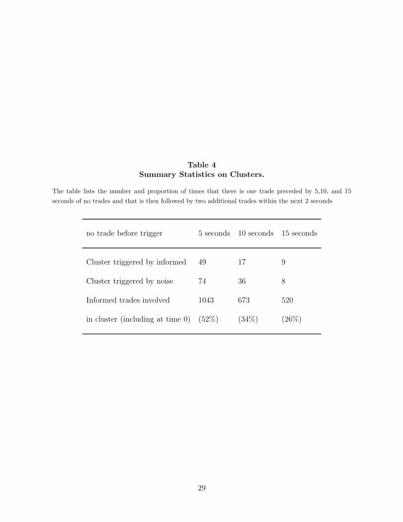
Table 4Summary Statistics on Clusters.

The table lists the number and proportion of times that there is one trade preceded by 5,10, and 15

seconds of no trades and that is then followed by two additional trades within the next 2 seconds

no trade before trigger 5 seconds 10 seconds 15 seconds

Cluster triggered by informed 49 17 9

Cluster triggered by noise 74 36 8

Informed trades involved 1043 673 520

in cluster (including at time 0) (52%) (34%) (26%)

29

Table 5The Probability of Being in a Cluster

The table shows the results from a logit regression of the probability of being in a cluster on a variety of explanatory variables. Standard errors are given

in parentheses below the coefficients; these are clustered at the group level.

No trading before the cluster 5 seconds 10 seconds 5 seconds 10 seconds 5 seconds 10 seconds 5 seconds 10 seconds

Triggering trade included? Yes Yes No No Yes Yes No No

Fixed effects included? No No No No Yes Yes Yes Yes

Herd -0.02559 -0.03687 -0.01303 -0.00341 0.00542 -0.0475 -0.00495 -0.01868(0.053) (0.041) (0.045) (0.033) (0.075) (0.051) (0.062) (0.041)

Contrarian -0.02089 -0.01409 0.00656 -0.00484 0.045 0.01533 0.04853 0.00636(0.051) (0.041) (0.043) (0.036) (0.064) (0.049) (0.052) (0.036)

U-shaped signal 0.17797*** 0.02459 0.11308* 0.01415 0.15349** 0.00567 0.08459 -0.01217(0.066) (0.043) (0.060) (0.037) (0.075) (0.055) (0.067) (0.047)

decreasing signal 0.15648** 0.02938 0.08132 0.00855 0.12771 -0.02346 0.04732 -0.0369(0.065) (0.044) (0.060) (0.037) (0.078) (0.055) (0.070) (0.046)

Increasing signal 0.08914 0.00974 0.03323 -0.00887 0.10883 -0.00678 0.07149 -0.01268(0.073) (0.049) (0.066) (0.042) (0.084) (0.057) (0.071) (0.042)

Same trade as preceding trade -0.01329 -0.00784 0.00535 0.0028 -0.02781 -0.00499 -0.0016 0.00983(0.030) (0.022) (0.024) (0.017) (0.036) (0.027) (0.027) (0.019)

Round-trip trade 0.02146 -0.01007 -0.01806 -0.03028 0.03941 -0.03717 -0.01708 -0.06048*(0.038) (0.030) (0.035) (0.026) (0.065) (0.044) (0.054) (0.036)

Constant -0.32155*** -0.21958*** -0.28725*** -0.17001*** 0.14636** 0.14729*** 0.11436* 0.11236***(0.060) (0.039) (0.054) (0.035) (0.069) (0.048) (0.059) (0.039)

Observations 996 996 996 996 996 996 996 996

30

Table 6Return Trades.

The table lists summary statistics for return (or round-trip) transactions. Row 1 lists the total trades

by types in treatments 4-6 (where two trades are possible). Row 2 lists the number of trades that were

first trades. Row 3 lists the number of second trades. A discrepancy between Row 2 and 3 indicates that

some people choose not to trade twice (Row 4). Row 5 lists how many of the second trades were classified

as return trades (buy-sell or sell-buy). Row 6 lists how many of the return trades lead to an immediate

trading profit. Row 7 lists the extend of buy-sell transactions (the remainder are sell-buy). Row 8 lists

whether the first trade was in the same direction as prices thus far (i.e. did prices rise and was the first

trade a buy or did prices fall and the first trade was a sale). Row 9 computes the same as Row 8 for the

second trade. Some “trades” were “passes”. For this table we count only the transactions; percentages

in rows 5-7 do not add to one as there may be passes. (This affected 55 “trades”. Specifically, there were

16 buy-holds, 22 sell-hold, 7 hold-sells, and 7 hold-holds. Most buy-holds (9) stemmed from S3 types,

most sell-holds (9) stemmed from S1 types.)

decreasing increasing hill-shape pU-shape nU-shape All

Total trades 425 373 146 183 181 1308

First trades 222 190 76 94 92 674

Second trades 203 183 70 89 89 634

Percent foregone 9% 4% 8% 3% 5% 6%

buy-buy 7 130 9 37 14 1973% 68% 12% 39% 15% 31%

sell-sell 146 8 28 11 46 23966% 4% 37% 12% 50% 38%

Return trades 36 29 25 33 20 14318% 16% 36% 37% 22% 23%

Profitable return 29 19 20 25 15 10881% 66% 80% 76% 75% 76%

buy-sell 17 21 14 22 15 5447% 72% 56% 67% 75% 72%

1st trade with price 14 20 7 22 15 78(p ր ⇒ buy) 39% 69% 28% 67% 75% 55%

2nd trade with price 15 7 5 8 5 40(p ր ⇒ buy) 42% 24% 20% 24% 25% 28%

31

Table 7Impact of Return Trades on Herding and Contrarianism.

The table condenses six regressions of the equations in lines (5) and (6) (by signal type and then with

respect to herding and contrarian behaviour separately). When cells are empty, there was insufficient data

or the variable was dropped. Constants were omitted from the report. Standard errors and significance

levels are denoted as in Table 2.

Herding Contrarian

U-shaped signal 0.14067***(0.03979)

return × U-shaped signal -0.10634**(0.04417)

Hill-shaped signal 0.39800***(0.11415)

return × Hill-shaped signal -0.1513(0.15627)

Return 0.22477*** 0.37721***0.02003 0.02619

Constant -0.28673*** -0.33828***(0.01383) (0.01315)

Observations 764 489

32

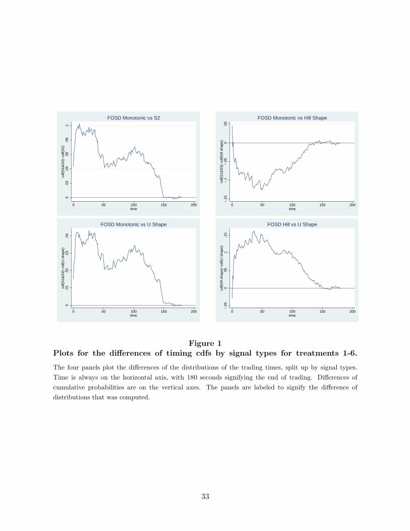
0.0

2.0

4.0

6.0

8.1

cdf(

S1&

S3)

−cd

f(S

2)

0 50 100 150 200time

FOSD Monotonic vs S2

−.1

5−

.1−

.05

0.0

5cd

f(S

1&S

3)−

cdf(

hill

shap

e)

0 50 100 150 200time

FOSD Monotonic vs Hill Shape

0.0

1.0

2.0

3.0

4cd

f(S

1&S

3)−

cdf(

U s

hape

)

0 50 100 150 200time

FOSD Monotonic vs U Shape−

.05

0.0

5.1

.15

cdf(

hill

shap

e)−

cdf(

U s

hape

)

0 50 100 150 200time

FOSD Hill vs U Shape

Figure 1Plots for the differences of timing cdfs by signal types for treatments 1-6.

The four panels plot the differences of the distributions of the trading times, split up by signal types.

Time is always on the horizontal axis, with 180 seconds signifying the end of trading. Differences of

cumulative probabilities are on the vertical axes. The panels are labeled to signify the difference of

distributions that was computed.

33

−.0

8−

.06

−.0

4−

.02

0.0

2cd

f(T

1−T

3)−

cdf(

T4−

T6)

0 50 100 150 200time

FOSD T1−T3 vs T4−T6, all trades

−.3

−.2

−.1

0cd

f(T

1−T

3)−

cdf(

T4−

T6,

1st

)

0 50 100 150 200time

FOSD T1−T3 vs T4−T6, 1st trade0

.05

.1.1

5.2

cdf(

T1−

T3)

−cd

f(T

4−T

6, 2

nd)

0 50 100 150 200time

FOSD T1−T3 vs T4−T6, 2nd trade

Figure 2Plots for the timing cdfs by number of trades.

The three panels plot distributions of the trading times, split up by treatments with one and two trades.

Axes are as in Figure 1. The top panel plots the cumulative probabilities for all trades; trades in

treatments 4-6 occur (weakly) before those in treatments 1-3. The bottom left panel looks only the

distribution of the first trades in treatments 4-6 and all the trades in treatments 1-3: trading occurs

earlier in treatments 4-6. The bottom right panel looks only at the distribution of the second trades in

treatments 4-6 and all the trades in treatments 1-3: trading occurs earlier in treatments 1-3.

34