Help for Smith V4 - fritz.dellsperger.net Smith/Help V4.1 -print.pdf · Smith-Chart Activate...

Help for Smith V4.1

Circuit Design with

Smith Chart

www.fritz.dellsperger.net

January 2018

http://www.fritz.dellsperger.net/

Content Help for Smith V4.1 ................................................................................................................................. 1 Overview .................................................................................................................................................. 1 Smith-Chart.............................................................................................................................................. 2

Menu and Toolbar ............................................................................................................................... 5 Input of Datapoints .............................................................................................................................. 7 Input of Circuit Elements for the Network ........................................................................................... 9 Circuit Elements ................................................................................................................................ 11

Edit circuit element values ............................................................................................................ 11 Tune circuit element values, Tuning Cockpit ................................................................................ 12 Capacitor (Serial or parallel element)..................................................................................... 14 Inductor (Serial or parallel element)..................................................................................... 15 Resistor (Serial or parallel element)..................................................................................... 16 Physical Transmission Line (Serial element) ................................................................... 17 Open ended Transmission Line, Open Stub (Parallel element) .................................. 19 Shorted Transmission Line, Shorted Stub (Parallel element) ...................................... 21 Transformer (Serial element) ................................................................................................. 23 R-L-C parallel connected (Serial element)......................................................................... 25 R-L-C serial connected (Parallel element) ......................................................................... 26

Edit Datapoints .................................................................................................................................. 27 Zoom-Function .................................................................................................................................. 27 Undo and Redo ................................................................................................................................. 28 Sweeps .............................................................................................................................................. 28 Circles ............................................................................................................................................... 31

Constant Q-Circles ........................................................................................................................ 31 Constant Gain Circles ................................................................................................................... 33 Constant VSWR Circles ................................................................................................................ 35 Stability-Circles ............................................................................................................................. 36 Constant Noise Figure Circles ...................................................................................................... 37

Settings ............................................................................................................................................. 39 Print the Smith-Chart ......................................................................................................................... 41 Copy to Clipboard.............................................................................................................................. 42 Shortcuts ........................................................................................................................................... 42 Save Netlist ....................................................................................................................................... 43 Export Data ....................................................................................................................................... 44

S-Plot ..................................................................................................................................................... 45 Export ................................................................................................................................................ 49

Export H-, Z-, Y- and A-Parameter to File .................................................................................... 49 Export CITI to S-Parameter Touchstone File ............................................................................... 51 Export S11 or S22 to smith chart .................................................................................................. 51

Print S-Plot ........................................................................................................................................ 53 Copy to Clipboard.............................................................................................................................. 54

Smith-Chart Basics ................................................................................................................................ 55 Smith-Chart Construction .................................................................................................................. 55

Stability Circles ............................................................................................................................. 58 Constant Gain Circles ................................................................................................................... 62 Simultaneous Conjugate Match .................................................................................................... 70 Constant Noise Figure Circles ...................................................................................................... 71

File format info ....................................................................................................................................... 72 Touchstone

® ...................................................................................................................................... 72

CITI .................................................................................................................................................... 74 EZNEC .............................................................................................................................................. 76

References ............................................................................................................................................ 77 License, Demoversion and Contact ...................................................................................................... 78 It’s a long way to a perfect software... ................................................................................................... 79 History .................................................................................................................................................... 80

1

Overview

The software is split in two parts: Smith-Chart and S-Plot Smith-Chart

Features:

Matching ladder networks with capacitors, inductors, resistors, transformers, serial

transmission lines and open or shorted stubs

Free settable normalization impedance for the Smith-Chart

Circles and contours for stability, noise figure, gain, VSWR and Q

Edit element values after insertion

Tune element values using sliders (Tuning Cockpit) new in V4.0

Sweep versus frequency or datapoints

Serial transmission line with loss

Export datapoint and circle info to ASCII-file for post-processing in spreadsheets or math software

Import datapoints from S-parameter files (Touchstone, CITI, EZNEC)

Undo- and Redo-Function

Save and load designs (licensed version only)

Print Smith-Chart, schematic, datapoints, circles and S-Plot graphs

Copy to clipboard for documentation purposes

Settings for color and line widths for all graphs

S-Plot

Features:

Read S-Parameter - Files in Touchstone

® -, CITI- and EZNEC- Format

Graphical display of s11, s12, s21 and s22

Graphical display and listing of MAG. (maximum operating power gain), MSG (maximum stable gain), stability factor k, µ and returnloss.

Linear or logarithmic frequency axis.

Cursor readout at gain and return loss graphs.

Convert and export S-Parameter to normalized or unnormalized H-, Z-, Y- or A-Parameters in Touchstone® - Format files.

Export s11 or s22 to Smith-Chart

Print all graphics or listings

System requirements: Windows Vista, Windows 7, 8, 10 .NET Framework 4.6.1 or higher

2

Smith-Chart Activate Smith-Chart in menu „Mode“ or

toggle between “S-Plot” and “Smith-Chart” with

The display has following features:

Smith-Chart Use the Smith-Chart the same way as on paper. Additionally comfortable tools like circles and locus are available. Window can be resized and moved to any position on display. Size and position of windows are saved on exit. Datapoints input with mouse, keyboard or from S-parameter file are labeled with DPn. n is the number of datapoint, starting with number 1. Datapoints transformed by circuit elements are labeled with TPm. m is the number of transformed datapoint, starting with nmax+1. Transformed datapoints resulting from sweeps are labeled with SPp. p is the number of transformed datapoint, starting with 1.

3

Schematic-window

Networks on Smith-Chart are displayed as schematics. Window can be resized and moved to any position on display. Size and position of windows are saved on exit.

Datapoint from which network is starting

In “Tools - Settings” the schematic can be rotated to vertical.

Datapoint from which network is starting

4

Datapoints-window Values for all datapoints are listed here. Window can be resized and moved to any position on display. Size and position of windows are saved on exit. Datapoints input with mouse, keyboard or from S-parameter file are labeled with DPn. n is the number of datapoint, starting with number 1. Datapoints transformed by circuit elements are labeled with TPm. m is the number of transformed datapoint, starting with nmax+1. Transformed datapoints resulting from sweeps are labeled with SPp. p is the number of transformed datapoint, starting with 1.

Circles-window Information of all circles is listed here. Window can be resized and moved to any position on display. Size and position of windows are saved on exit.

Gn = Gain circle number n Sn = Stability circle number n Nn = Noise circle number n

Cursor-window

Display of actual values for the mouse cursor (Return Loss, VSWR, Q, (Gamma), Admittance Y, Impedance Z, normalizing impedance Z0 and Frequency of datapoint from which network is starting).

5

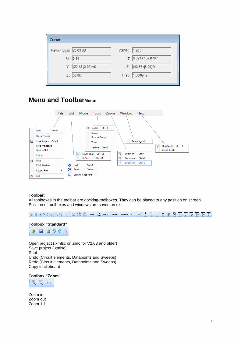
Menu and ToolbarMenu:

Toolbar: All toolboxes in the toolbar are docking-toolboxes. They can be placed to any position on screen. Position of toolboxes and windows are saved on exit.

Toolbox “Standard”

Open project (.xmlsc or .smc for V2.03 and older) Save project (.xmlsc) Print Undo (Circuit elements, Datapoints and Sweeps) Redo (Circuit elements, Datapoints and Sweeps) Copy to clipboard Toolbox “Zoom”

Zoom in Zoom out Zoom 1:1

6

Toolbox “Mode, circles and settings”

Toggle between Smith-Chart and S-Plot Open Circles Dialogbox Open Settings Open Sweep Dialogbox Clear Sweep Open Tuning Cockpit Toolbox “Datapoints”

Input Datapoint

Mouse

Keyboard

S11 from file

S22 from file

Toolbox “Elements”

Insert Serial Element

Capacitor

Inductor

Resistor

Transmission Line

Transformer

R-L-C

Insert Parallel Element

Capacitor

Inductor

Resistor

Open Stub

Shorted Stub

R-L-C

7

Input of Datapoints

There are four options to input datapoints:

Input Datapoint

Mouse

Keyboard

S11 from file

S22 from file

Input with mouse:

Select „Mouse“ in toolbox. This is a toggle-function ON/OFF. The button color turns to green for ON, blue for OFF.

Move mouse cursor to desired datapoint in Smith-Chart. Watch window Cursor for actual data values.

Left mouse click sets datapoint.

Enter frequency in dialogbox.

Continue with input of next datapoint.

Terminate datapoint input with clicking to “Mouse”-button in toolbox (color turns back to blue) or select a circuit-element

Input with Keyboard:

Select „Keyboard“

Enter values in dialogbox. Data can be input as impedance, admittance or reflection coefficient in cartesian or polar notation. Enter frequency in dialogbox.

Import from S-Parameter Data File: Datapoints can be imported from S-Parameter files or exported from S-Plot. See „S-Plot, Export to Smith Chart„. S-Parameter file can be in Touchstone-, CITI- or EZNEC-format.

Click on „S11“ or „S22“.

8

Select File.

Choose file format: Touchstone format (*.s1p, *.s2p) CITI format (*.citi, *.cti) EZNEC format (*.txt)

9

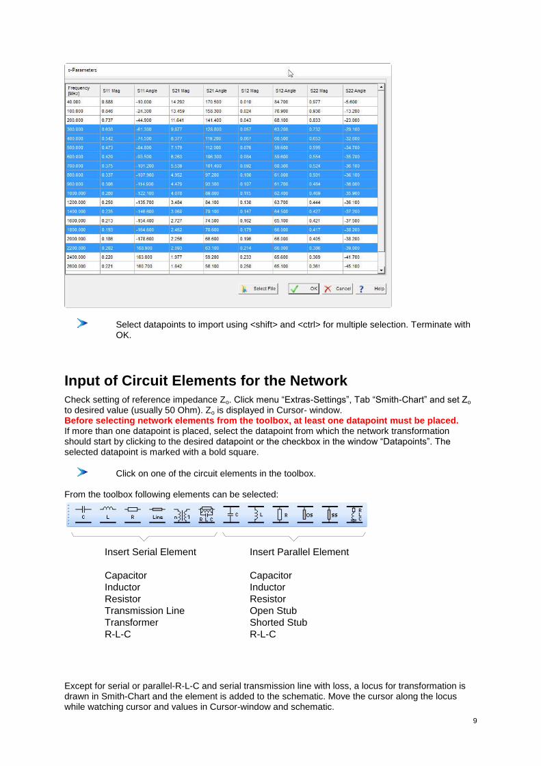
Select datapoints to import using <shift> and <ctrl> for multiple selection. Terminate with OK.

Input of Circuit Elements for the Network

Check setting of reference impedance Zo. Click menu “Extras-Settings”, Tab “Smith-Chart” and set Zo

to desired value (usually 50 Ohm). Zo is displayed in Cursor- window. Before selecting network elements from the toolbox, at least one datapoint must be placed. If more than one datapoint is placed, select the datapoint from which the network transformation should start by clicking to the desired datapoint or the checkbox in the window “Datapoints”. The selected datapoint is marked with a bold square.

Click on one of the circuit elements in the toolbox. From the toolbox following elements can be selected:

Insert Serial Element

Capacitor

Inductor

Resistor

Transmission Line

Transformer

R-L-C

Insert Parallel Element

Capacitor

Inductor

Resistor

Open Stub

Shorted Stub

R-L-C

Except for serial or parallel-R-L-C and serial transmission line with loss, a locus for transformation is drawn in Smith-Chart and the element is added to the schematic. Move the cursor along the locus while watching cursor and values in Cursor-window and schematic.

10

Click at desired value. This terminates the element insertion. For RLC, input element values in dialogbox.

Undo with right mouse button if desired.

Change element value by double-clicking on element or element-value in Schematic-window.

Serial transmission line:

If attenuation is 0 dB/m a locus for transformation is drawn in Smith-Chart and the element is added to the schematic. Move the cursor along the locus while watching cursor and values in Cursor-window and schematic.

If attenuation is >0 dB/m the line length in must be defined. No locus for cursor moving is drawn on Smith-Chart.

11

Circuit Elements

Edit circuit element values To edit circuit element values:

Double-click on element or element-value in Schematic-window.

Change value in dialogbox and click “Draw”. All calculations are redone and the Smith-Chart is updated.

Change values

Click Draw and watch Smith-chart,

schematic and window „Datapoints“ how

this affect transformation

OK when done

Do not use values of 0 (zero), instead input a very small value, e.g. 0.000001. In some special cases a value of 0 can cause an error.

12

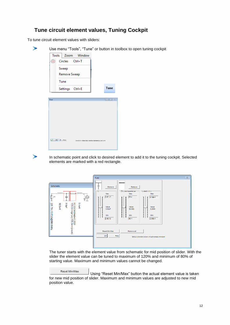
Tune circuit element values, Tuning Cockpit To tune circuit element values with sliders:

Use menu “Tools”, “Tune” or button in toolbox to open tuning cockpit

In schematic point and click to desired element to add it to the tuning cockpit. Selected elements are marked with a red rectangle.

The tuner starts with the element value from schematic for mid position of slider. With the slider the element value can be tuned to maximum of 120% and minimum of 80% of starting value. Maximum and minimum values cannot be changed.

Using “Reset Min/Max” button the actual element value is taken for new mid position of slider. Maximum and minimum values are adjusted to new mid position value.

13

Before “Reset Min/Max”

After “Reset Min/Max”

Move slider and watch Smith-Chart

Remove element from tuning cockpit with remove button.

Remove all elements from tuning cockpit.

For final closing of tuning cockpit and terminate all tuning functions remove all elements in Tune window. The red marking rectangles of the elements in schematic are deleted.

14

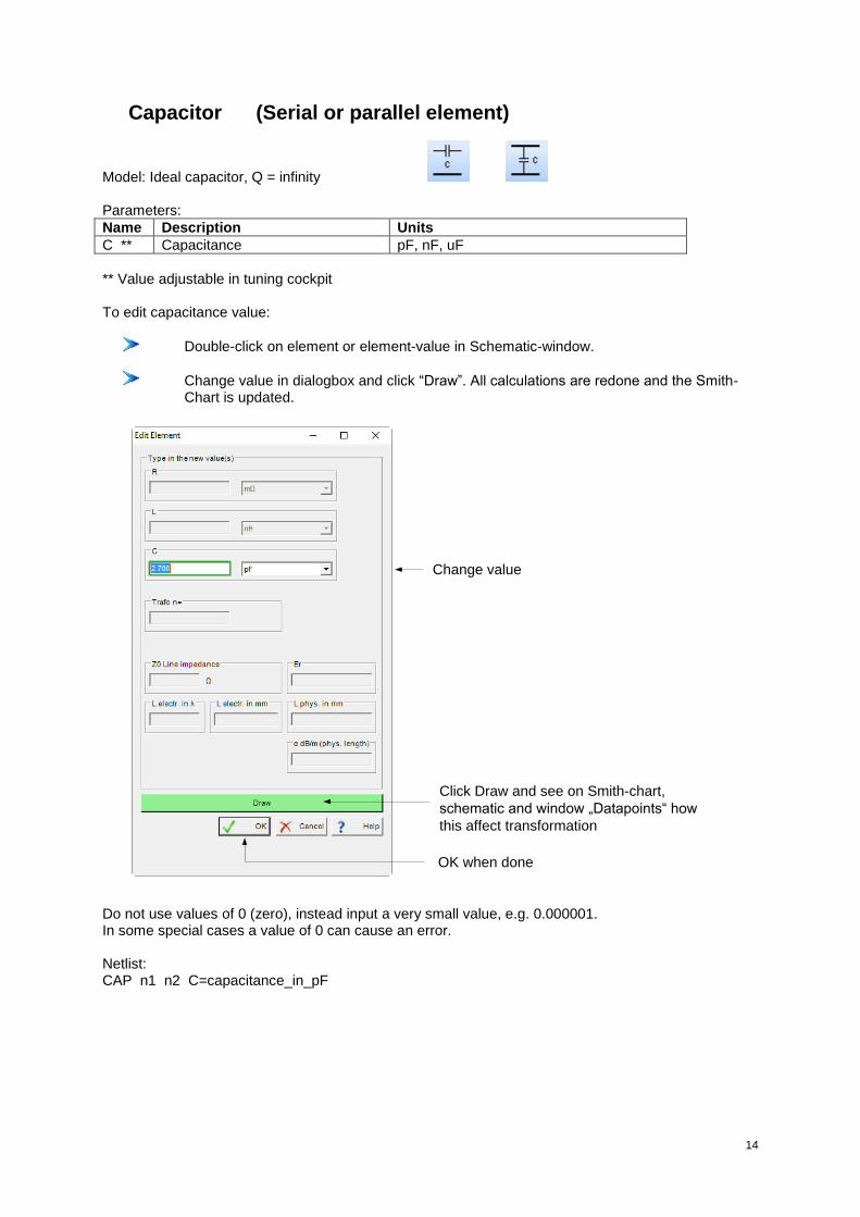
Capacitor (Serial or parallel element)

Model: Ideal capacitor, Q = infinity Parameters:

Name Description Units

C ** Capacitance pF, nF, uF

** Value adjustable in tuning cockpit To edit capacitance value:



Change value

Click Draw and see on Smith-chart,



OK when done

Do not use values of 0 (zero), instead input a very small value, e.g. 0.000001. In some special cases a value of 0 can cause an error. Netlist: CAP n1 n2 C=capacitance_in_pF

15

Inductor (Serial or parallel element)

Model: Ideal inductor, Q = infinity Parameters:


L ** Inductance pH, nH, uH

** Value adjustable in tuning cockpit To edit inductance value:



Change value




OK when done

Do not use values of 0 (zero), instead input a very small value, e.g. 0.000001. In some special cases a value of 0 can cause an error. Netlist: IND n1 n2 L=iductance_in_nH

16

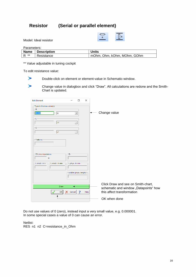
Resistor (Serial or parallel element)

Model: Ideal resistor Parameters:


R ** Resistance mOhm, Ohm, kOhm, MOhm, GOhm

** Value adjustable in tuning cockpit To edit resistance value:



Change value




OK when done

Do not use values of 0 (zero), instead input a very small value, e.g. 0.000001. In some special cases a value of 0 can cause an error. Netlist: RES n1 n2 C=resistance_in_Ohm

17

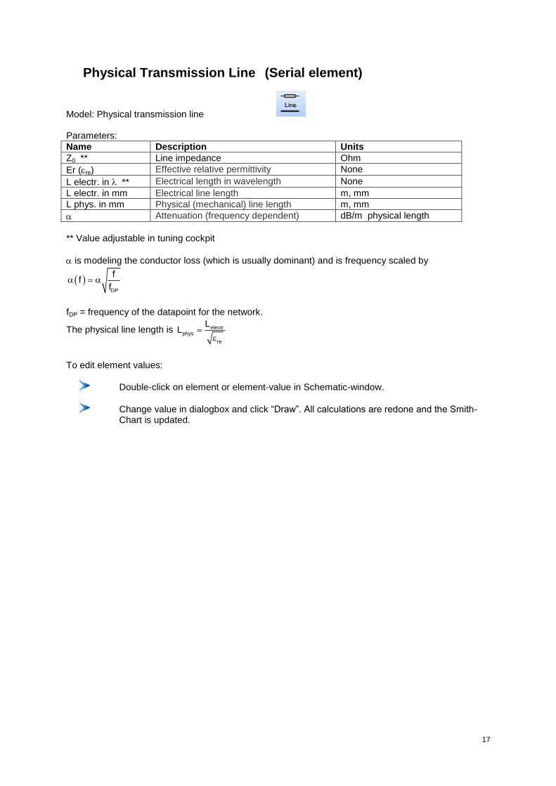
Physical Transmission Line (Serial element)

Model: Physical transmission line Parameters:


Z0 ** Line impedance Ohm

Er (re) Effective relative permittivity None

L electr. in ** Electrical length in wavelength None

L electr. in mm Electrical line length m, mm

L phys. in mm Physical (mechanical) line length m, mm

Attenuation (frequency dependent) dB/m physical length

** Value adjustable in tuning cockpit

is modeling the conductor loss (which is usually dominant) and is frequency scaled by

DP

ff

f

fDP = frequency of the datapoint for the network.

The physical line length is electrphys

re

LL

To edit element values:



18

Change values




OK when done

Do not use values of 0 (zero), instead input a very small value, e.g. 0.000001. In some special cases a value of 0 can cause an error. Netlist: TLINP n1 n2 n3 Z=line_imp_in_Ohm L=length_elec_in_mm K=eff_dielectric_const_Ere A=attenuation_in_dB/m F=0

n1

n3 n3

n2

Z, L, K, A, F

n3=0

Remark on relative permittivity (relative dielectric constant) r using lines:

If the line consist of microstrip, stripline or other planar line, use effective relative permittivity re .

re is a function of substrate r , W/h, t and frequency.

For microstrip lines it can be approximated by

0.555

0 0

1 11 10 / 1

2 2r r

re

t f

hw h

w

Sometime instead of r the relative velocity rv is used.

rv is related to r by

1r

r

v

19

Open ended Transmission Line, Open Stub (Parallel element)

Model: Ideal transmission line Parameters:



Er Effective dielectric constant None






re

LL




Change values




OK when done


20

Netlist: TLINP n1 n2 n3 Z=line_imp_in_Ohm L=length_elec_in_mm K=eff_dielectric_const_Ere A=0 F=0

n1

n3 n3

n2

Z, L, K, A, F

n2=99 n3=0





0.555

0 0

1 11 10 / 1

2 2r r

re

t f

hw h

w



1r

r

v

21

Shorted Transmission Line, Shorted Stub (Parallel element)

Model: Ideal transmission line Parameters:



Er Effective dielectric constant None






re

LL




Change values




OK when done


22

Netlist: TLINP n1 n2 n3 Z=line_imp_in_Ohm L=length_elec_in_mm K=eff_dielectric_const_Ere A=0 F=0

n1

n3 n3

n2

Z, L, K, A, F

n2=0 n3=0





0.555

0 0

1 11 10 / 1

2 2r r

re

t f

hw h

w



1r

r

v

23

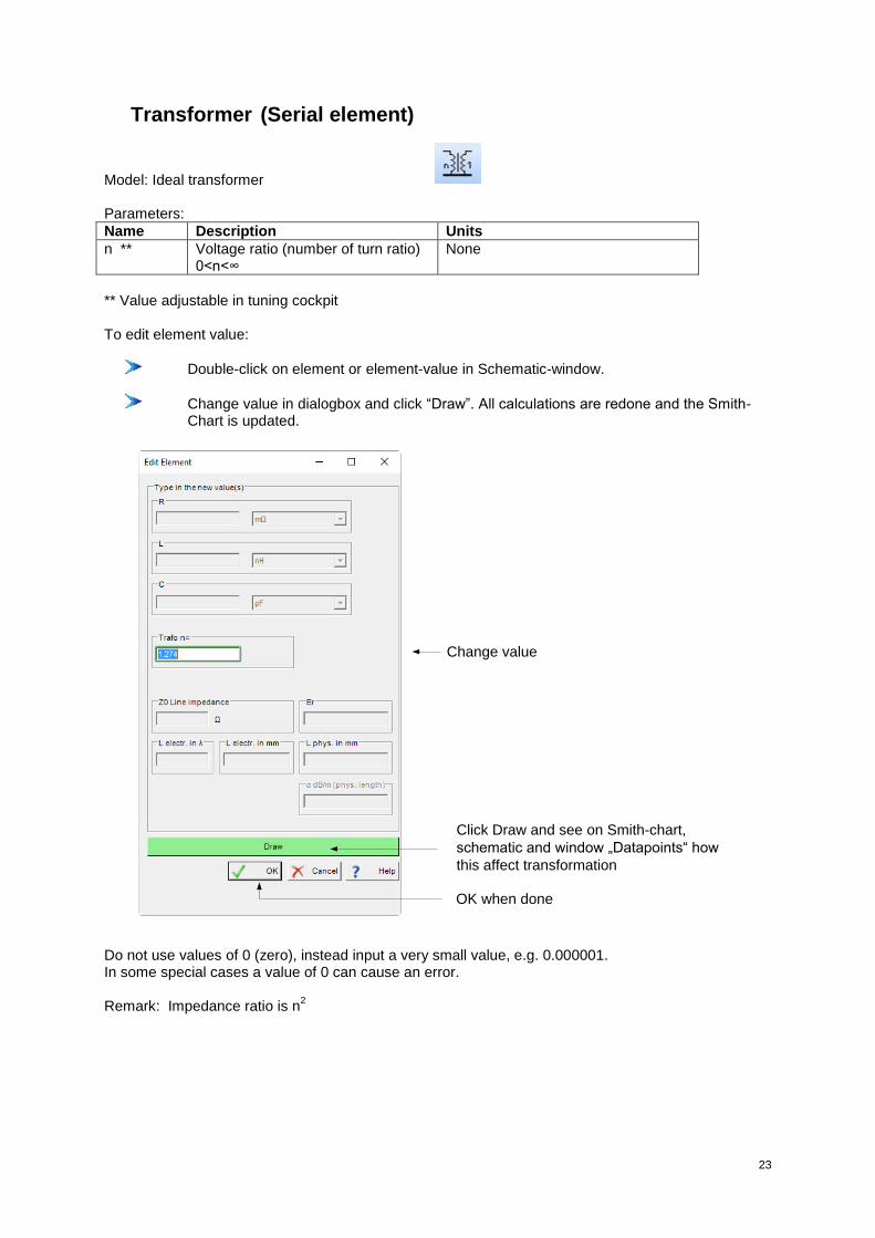
Transformer (Serial element)

Model: Ideal transformer Parameters:


n ** Voltage ratio (number of turn ratio) 0<n<∞

None

** Value adjustable in tuning cockpit To edit element value:



Change value




OK when done

Do not use values of 0 (zero), instead input a very small value, e.g. 0.000001. In some special cases a value of 0 can cause an error. Remark: Impedance ratio is n

2

24

Netlist: TRF n1 n2 n3 n4 N=turns_ratio R1=0

n1

n3 n4

n2

N:1

R1

n3=0 n4=0 R1=0

25

R-L-C parallel connected (Serial element)

Model: Ideal Resistor, Inductor and Capacitor parallel connected Parameters:


R ** Resistance Ohm, kOhm, MOhm



** Value adjustable in tuning cockpit To edit element values:



Change values




OK when done

Do not use values of 0 (zero), instead input a very small value, e.g. 0.000001. In some special cases a value of 0 can cause an error. Netlist: PRLC n1 n2 R=resistance_in_Ohm L=inductance_in_nH C=capacitance_in_pF

26

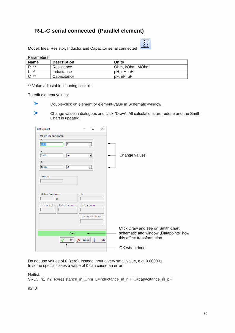
R-L-C serial connected (Parallel element)

Model: Ideal Resistor, Inductor and Capacitor serial connected Parameters:


R ** Resistance Ohm, kOhm, MOhm



** Value adjustable in tuning cockpit To edit element values:



Change values




OK when done

Do not use values of 0 (zero), instead input a very small value, e.g. 0.000001. In some special cases a value of 0 can cause an error. Netlist: SRLC n1 n2 R=resistance_in_Ohm L=inductance_in_nH C=capacitance_in_pF n2=0

27

Edit Datapoints

Double-click on datapoint in Smith-Chart.

Change values in dialogbox. All calculations are redone and the Smith-Chart updated.

Zoom-Function

Use menu “Zoom” or shortcuts or buttons in toolbox.

There are 3 options for zooming:

“Zoom in” Shortcut “Ctrl+1”

“Zoom out” Shortcut “Ctrl+2”

“Zoom 1:1” Shortcut “Ctrl+3”

The center of zoom is always the center of the Smith-Chart.

28

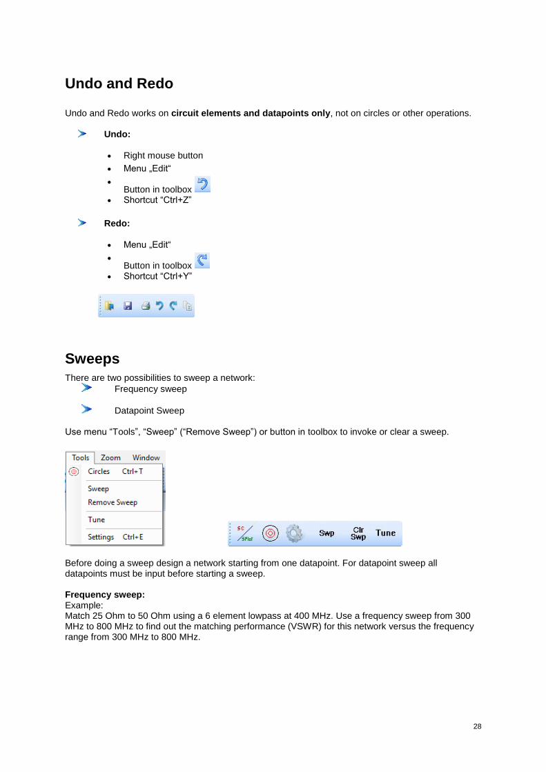
Undo and Redo

Undo and Redo works on circuit elements and datapoints only, not on circles or other operations.

Undo:

Right mouse button

Menu „Edit“

Button in toolbox

Shortcut “Ctrl+Z”

Redo:

Menu „Edit“

Button in toolbox

Shortcut “Ctrl+Y”

Sweeps

There are two possibilities to sweep a network:

Frequency sweep

Datapoint Sweep

Use menu “Tools”, “Sweep” (“Remove Sweep”) or button in toolbox to invoke or clear a sweep.

Before doing a sweep design a network starting from one datapoint. For datapoint sweep all datapoints must be input before starting a sweep. Frequency sweep: Example: Match 25 Ohm to 50 Ohm using a 6 element lowpass at 400 MHz. Use a frequency sweep from 300 MHz to 800 MHz to find out the matching performance (VSWR) for this network versus the frequency range from 300 MHz to 800 MHz.

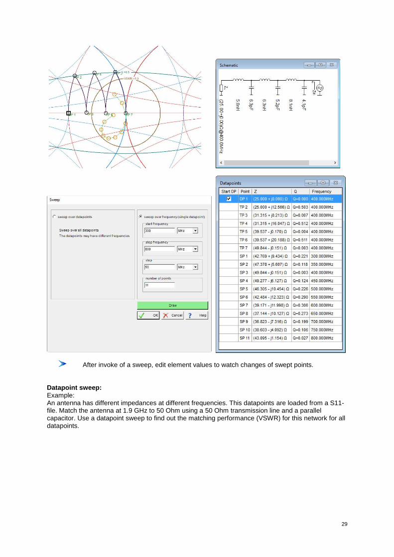
29

After invoke of a sweep, edit element values to watch changes of swept points. Datapoint sweep: Example: An antenna has different impedances at different frequencies. This datapoints are loaded from a S11-file. Match the antenna at 1.9 GHz to 50 Ohm using a 50 Ohm transmission line and a parallel capacitor. Use a datapoint sweep to find out the matching performance (VSWR) for this network for all datapoints.

30

After invoke of a sweep, edit element values to watch changes of swept points.

31

Circles

Use menu „Tools“, „Circles“ or shortcut “Ctrl+T” or button in toolbox.

There are following options:

Q-Circles Gain-Circles VSWR-Circles Stability-Circles Noise Figure Circles

Constant Q-Circles

Select menu „Tools“, „Circles“ or shortcut “Ctrl+T”

or click button in toolbox and select tab „Q“

Enter Q for the locus This draws the locus (ellipse) of all points for

Im( ).

Re( )

ZQ const

Z .

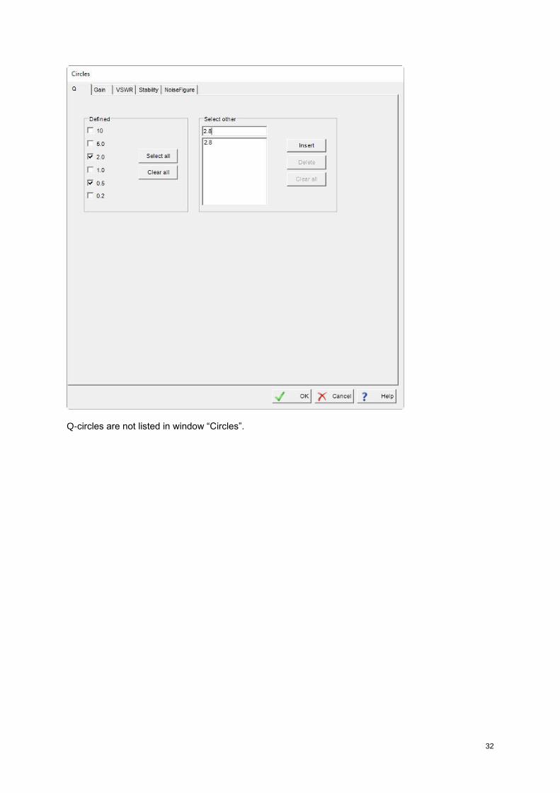
32

Q-circles are not listed in window “Circles”.

33

Constant Gain Circles


or click button in toolbox and select tab „Gain“.

Select “Available Power Gain”, “Operating Power Gain” or “Unilateral”. Use “Available Power Gain” for low noise amplifiers. Use “Operating Power Gain” for amplifiers with maximum output power, best efficiency or lowest intermodulation. Use “Unilateral” for first approximation of matching network.

Enter S-parameter or import parameter from a file.

Enter desired Gain for the circle (must be less than Gmax). If Stability factor K<1, Available Power Gain and Operating Power Gain are undefined and circles are for conditionally stable twoports. Be careful your amplifier may oscillate. One possibility to avoid oscillation is to stabilize the twoport in advance (serial or parallel resistor at input and/or output, until K>1). For unilateral devices S12 is assumed to be zero.

Click “Draw”.

Continue with entering gain for next circle. Click “Draw”, etc.

Constant Gain circles are labeled with „Gn“. n is the number of the circle, starting with number 1.

34

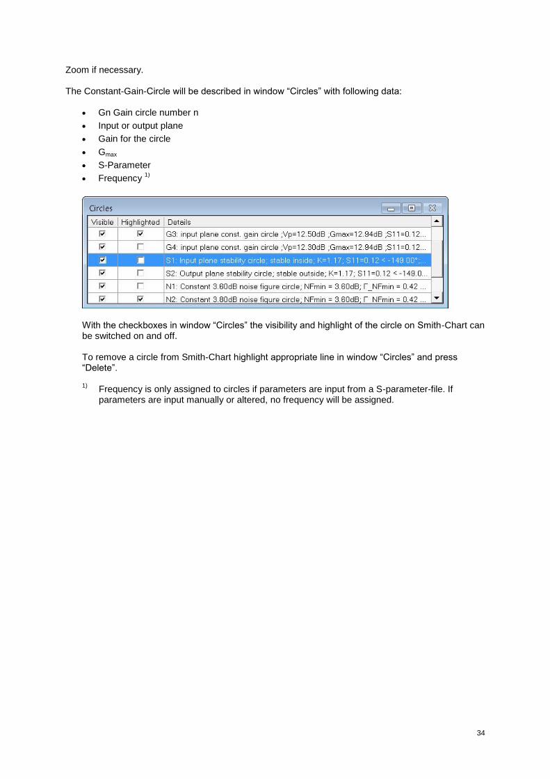
Zoom if necessary. The Constant-Gain-Circle will be described in window “Circles” with following data:

Gn Gain circle number n

Input or output plane

Gain for the circle

Gmax

S-Parameter

Frequency 1)

With the checkboxes in window “Circles” the visibility and highlight of the circle on Smith-Chart can be switched on and off. To remove a circle from Smith-Chart highlight appropriate line in window “Circles” and press “Delete”. 1)

Frequency is only assigned to circles if parameters are input from a S-parameter-file. If parameters are input manually or altered, no frequency will be assigned.

35

Constant VSWR Circles


or click button in toolbox and select tab „VSWR“

Enter VSWR for the circle The circles are always centered to the center of the Smith-Chart.

VSWR-circles are not listed in window “Circles”.

36

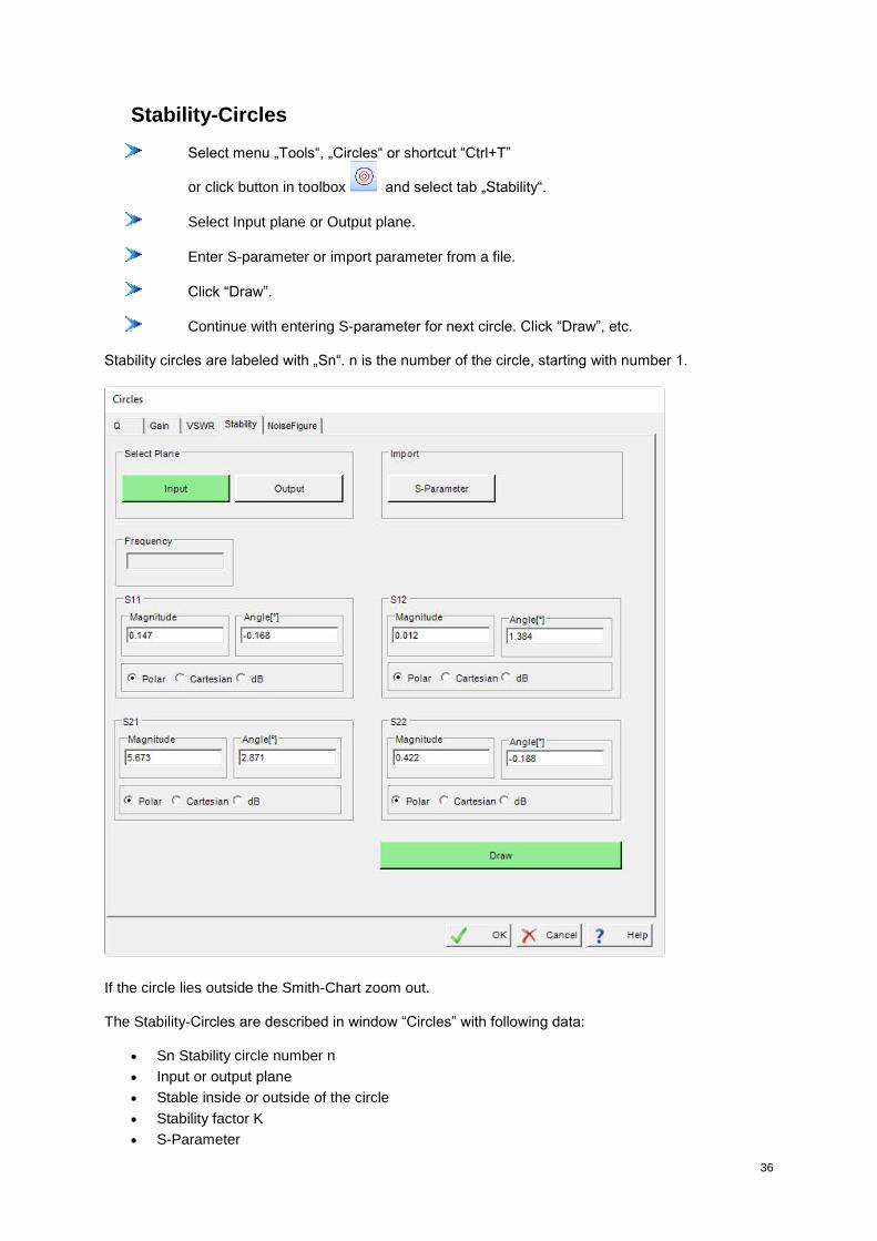
Stability-Circles


or click button in toolbox and select tab „Stability“.

Select Input plane or Output plane.

Enter S-parameter or import parameter from a file.

Click “Draw”.

Continue with entering S-parameter for next circle. Click “Draw”, etc. Stability circles are labeled with „Sn“. n is the number of the circle, starting with number 1.

If the circle lies outside the Smith-Chart zoom out. The Stability-Circles are described in window “Circles” with following data:

Sn Stability circle number n

Input or output plane

Stable inside or outside of the circle

Stability factor K

S-Parameter

37

Frequency 1)



Constant Noise Figure Circles


or click button in toolbox and select tab „Noise Figure“.

Enter noise data or import parmeter from a file:

Minimum noise figure NFmin in dB

G_ NFmin (reflection coefficient corresponding to NFmin)

Equivalent input noise resistance, normalized or unnormalized

Enter desired Noise figure NF for the circle in dB (>NFmin)

Click “Draw”.

Continue with entering NF for next circle. Click “Draw”, etc. Constant Noise Figure Circles are labeled with „Nn“. n is the number of the circle, starting with number 1.

38

Zoom if necessary. Remark: Touchstone files have normalized noise resistance info. CITI-files can have normalized or not normalized noise resistance info. Check appropriate radio button in window above. The Constant Noise Figure Circle will be described in window “Circles” with following data:

Nn Noise Figure circle number n

NF for the circle

NFmin

min_NF

Equivalent input noise resistance

Frequency 1)

39



Settings

Select menu „Tools“, „Settings“ or shortcut “Ctrl+E” or click button in toolbox

. Tab Smith-Chart

- Line width and colors - Zo for Smithchart - Default frequency for datapoint - Labels - Z-plane, Y-plane on/off

40

Tab S-Plot - Line width and colors - Labels - Z-plane, Y-plane on/off

Tab General

- Default start mode (Smith-Chart or S-Plot)

41

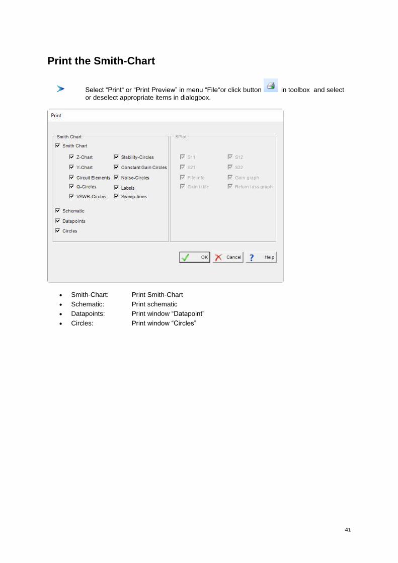
Print the Smith-Chart

Select “Print“ or “Print Preview” in menu “File“or click button in toolbox and select or deselect appropriate items in dialogbox.

Smith-Chart: Print Smith-Chart

Schematic: Print schematic

Datapoints: Print window “Datapoint”

Circles: Print window “Circles”

42

Copy to Clipboard

Select „Copy to Clipboard“ in menu „Edit“ or click button in toolbox and select appropriate item.

A copy of the selected item is put to the clipboard for insertion in office applications.

Shortcuts

Following shortcuts can be used for best productivity: File New Ctrl+N Open Ctrl+O Save Ctrl+S Edit Undo Ctrl+Z Redo Ctrl+Y Mode Toggle Smith-Chart/S-Plot Ctrl+M Tools Circles Ctrl+T Extras Settings Ctrl+E Zoom Zoom in Ctrl+1 Zoom out Ctrl+2 Zoom 1:1 Ctrl+3 Help Help F1

43

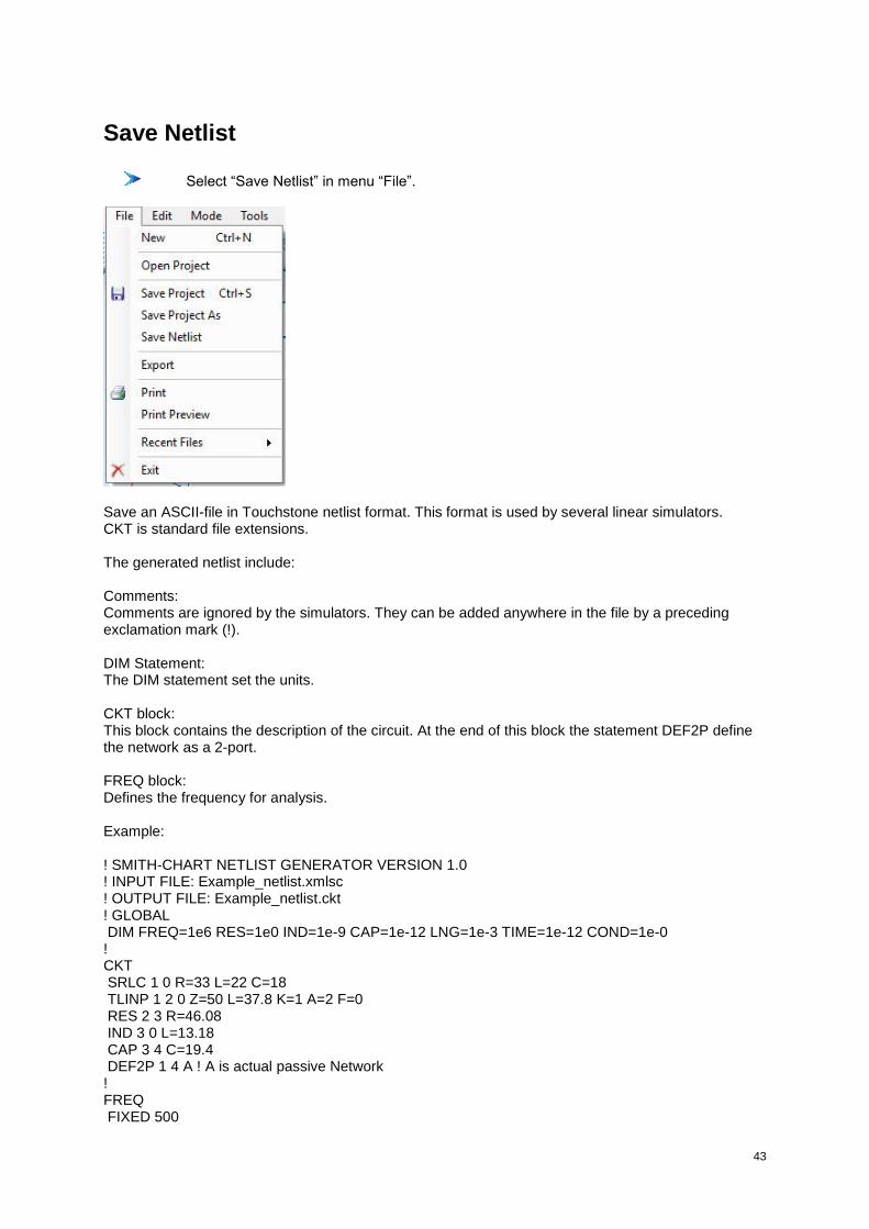
Save Netlist

Select “Save Netlist” in menu “File”.

Save an ASCII-file in Touchstone netlist format. This format is used by several linear simulators. CKT is standard file extensions. The generated netlist include: Comments: Comments are ignored by the simulators. They can be added anywhere in the file by a preceding exclamation mark (!). DIM Statement: The DIM statement set the units. CKT block: This block contains the description of the circuit. At the end of this block the statement DEF2P define the network as a 2-port. FREQ block: Defines the frequency for analysis. Example: ! SMITH-CHART NETLIST GENERATOR VERSION 1.0 ! INPUT FILE: Example_netlist.xmlsc ! OUTPUT FILE: Example_netlist.ckt ! GLOBAL DIM FREQ=1e6 RES=1e0 IND=1e-9 CAP=1e-12 LNG=1e-3 TIME=1e-12 COND=1e-0 ! CKT SRLC 1 0 R=33 L=22 C=18 TLINP 1 2 0 Z=50 L=37.8 K=1 A=2 F=0 RES 2 3 R=46.08 IND 3 0 L=13.18 CAP 3 4 C=19.4 DEF2P 1 4 A ! A is actual passive Network ! FREQ FIXED 500

44

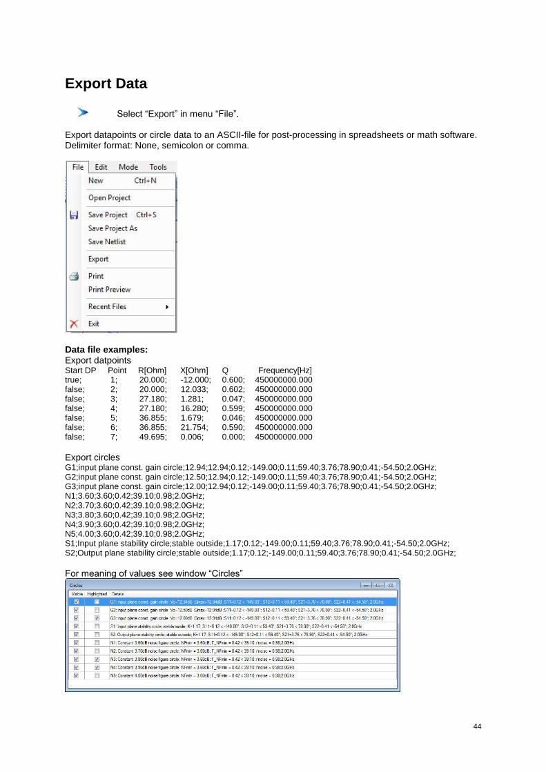
Export Data

Select “Export” in menu “File”. Export datapoints or circle data to an ASCII-file for post-processing in spreadsheets or math software. Delimiter format: None, semicolon or comma.

Data file examples:

Export datpoints

Start DP Point R[Ohm] X[Ohm] Q Frequency[Hz] true; 1; 20.000; -12.000; 0.600; 450000000.000

false; 2; 20.000; 12.033; 0.602; 450000000.000

false; 3; 27.180; 1.281; 0.047; 450000000.000

false; 4; 27.180; 16.280; 0.599; 450000000.000

false; 5; 36.855; 1.679; 0.046; 450000000.000

false; 6; 36.855; 21.754; 0.590; 450000000.000

false; 7; 49.695; 0.006; 0.000; 450000000.000

Export circles

G1;input plane const. gain circle;12.94;12.94;0.12;-149.00;0.11;59.40;3.76;78.90;0.41;-54.50;2.0GHz; G2;input plane const. gain circle;12.50;12.94;0.12;-149.00;0.11;59.40;3.76;78.90;0.41;-54.50;2.0GHz; G3;input plane const. gain circle;12.00;12.94;0.12;-149.00;0.11;59.40;3.76;78.90;0.41;-54.50;2.0GHz; N1;3.60;3.60;0.42;39.10;0.98;2.0GHz; N2;3.70;3.60;0.42;39.10;0.98;2.0GHz; N3;3.80;3.60;0.42;39.10;0.98;2.0GHz; N4;3.90;3.60;0.42;39.10;0.98;2.0GHz; N5;4.00;3.60;0.42;39.10;0.98;2.0GHz; S1;Input plane stability circle;stable outside;1.17;0.12;-149.00;0.11;59.40;3.76;78.90;0.41;-54.50;2.0GHz; S2;Output plane stability circle;stable outside;1.17;0.12;-149.00;0.11;59.40;3.76;78.90;0.41;-54.50;2.0GHz;

For meaning of values see window “Circles”

45

S-Plot

Export Print S-Plot

Read S-Parameter - Files in Touchstone® -, CITI- and EZNEC- Format and display the data in

different graphs and listings. Convert and export S-Parameter to normalized or unnormalized H-, Z-, Y- or A-Parameters in Touchstone® - Format files. Export s11 or s22 to Smith-Chart. Print all graphs or listings.

Select „S-Plot“ in menu „Mode“.

Load S-Parameter file with „Open“ in menu „File“.

46

Choose file format: Touchstone format (*.s1p, *.s2p) CITI format (*.citi, *.cti) EZNEC format (*.txt)

S11 and S22 are plotted to a Smith-Chart, S12 and S21 to a polar plot. There are additional windows for:

Source file

Gain table with listing of MAG[dB] (maximum available operating power gain), MSG[dB]

(maximum stable gain), stability factor K, stability factor s (Mue) and S12[dB]

Gain graph for MAG[dB] (for K1) and MSG[dB] (for K<1), stability factor K and stability factor

s (Mue)

Return Loss graph for S11[dB] and S22[dB] The selected line in window “Gain table” highlights the corresponding datapoint in all graphs.

48

Equations:

221

max

12

1 ; 1 p

SMAG G K K K

S

21

max

12

; 1 p stabil

SMSG G K

S

2 2 2

11 22

12 21

1

2

S SK

S S

11 22 12 21 S S S S

2

22

*

11 22 21 12

11

S

S

S S S S

1111[ ] 20logS dB S

2222[ ] 20logS dB S

1212[ ] 20logS dB S

49

Export

Export H-, Z-, Y- and A-Parameter to File Export CITI to S-Parameter Touchstone File Export S11 or S22 to Smith Chart

Export H-, Z-, Y- and A-Parameter to File After loading an S-Parameter file in S-Plot, the file can be converted to H-, Z-, Y- or A-Parameter (normalized or unnormalized) and saved in a file. All converted files are in Touchstone

® - Format.

Menu „Export“, „s- to x-parameter-file“.

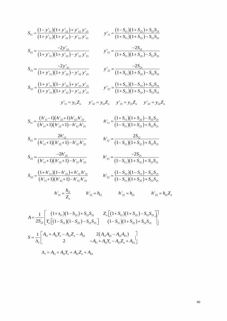
Equations Twoport Parameter Conversion

S-, Z-, Y-, H- and A(ABCD)-Parameter:

‘ (apostrophe) denotes normalized parameter.

11 22 12 21 11 22 12 21

11 11

11 22 12 21 11 22 12 21

' 1 ' 1 ' ' 1 1'

' 1 ' 1 ' ' 1 1

z z z z S S S SS z

z z z z S S S S

12 12

12 12

11 22 12 21 11 22 12 21

2 ' 2'

' 1 ' 1 ' ' 1 1

z SS z

z z z z S S S S

21 21

21 21

11 22 12 21 11 22 12 21

2 ' 2'

' 1 ' 1 ' ' 1 1

z SS z

z z z z S S S S

11 22 12 21 11 22 12 21

22 22

11 22 12 21 11 22 12 21

' 1 ' 1 ' ' 1 1'

' 1 ' 1 ' ' 1 1

z z z z S S S SS z

z z z z S S S S

11 12 21 2211 12 21 22' ' ' '

o o o o

z z z zz z z z

Z Z Z Z

50

11 22 12 21 11 22 12 21

11 11

11 22 12 21 11 22 12 21

1 ' 1 ' ' ' 1 1'

1 ' 1 ' ' ' 1 1

y y y y S S S SS y

y y y y S S S S

12 12

12 12

11 22 12 21 11 22 12 21

2 ' 2'

1 ' 1 ' ' ' 1 1

y SS y

y y y y S S S S

21 21

21 21

11 22 12 21 11 22 12 21

2 ' 2'

1 ' 1 ' ' ' 1 1

y SS y

y y y y S S S S

11 22 12 21 11 22 12 21

22 22

11 22 12 21 11 22 12 21

1 ' 1 ' ' ' 1 1'

1 ' 1 ' ' ' 1 1

y y y y S S S SS y

y y y y S S S S

11 11 12 12 21 21 22 22' ' ' ' o o o oy y Z y y Z y y Z y y Z

11 22 12 21 11 22 12 21

11 11

11 22 12 21 11 22 12 21

' 1 ' 1 ' ' 1 1'

' 1 ' 1 ' ' 1 1

h h h h S S S SS h

h h h h S S S S

12 12

12 12

11 22 12 21 11 22 12 21

2 ' 2'

' 1 ' 1 ' ' 1 1

h SS h

h h h h S S S S

21 21

21 21

11 22 12 21 11 22 12 21

2 ' 2'

' 1 ' 1 ' ' 1 1

h SS h

h h h h S S S S

11 22 12 21 22 11 12 21

22 22

11 22 12 21 11 22 12 21

1 ' 1 ' ' ' 1 1'

' 1 ' 1 ' ' 1 1

h h h h S S S SS h

h h h h S S S S

1111 12 12 21 21 22 22' ' ' ' o

o

hh h h h h h h Z

Z

11 22 12 21 11 22 12 21

21 11 22 12 21 11 22 12 21

1 1 1 11

2 1 1 1 1

o

o

s S S S Z S S S SA

S Y S S S S S S S S

11 12 21 22 11 22 12 21

1 11 12 21 22

21

2

o o

o o

A A Y A Z A A A A AS

A A Y A Z A

1 11 12 21 22 o oA A Y A Z A

51

Export CITI to S-Parameter Touchstone File A CITI-file loaded in S-Plot can be saved as S-parameter file in Touchstone format.

Menu „Export“, „CITI- to S“.

Export S11 or S22 to smith chart

Menu „Export“, „s11 (or s22) to smith chart“.

52

Select appropriate parameter lines using <Shift> and <Ctrl> for multiple selection. Terminate with OK.

53

Print S-Plot

Select “Print“ or “Print Preview” in menu “File“or click button in toolbox and select or deselect appropriate items in dialogbox.

S11, S12, S21, S22: Print window S11, S12, S21, S22

Gain table: Print Gain table

Gain graph: Print Gain graph

Return loss graph: Print Return loss graph

54

Copy to Clipboard

Select „Copy to Clipboard“ in menu „Edit“ or click button in toolbox and select appropriate item.

A copy of the selected item is put to the clipboard for insertion in office applications.

55

Smith-Chart Basics

Smith-Chart Construction Stability Circles

Source Stability Circles Load Stability Circles

Constant Gain Circles Transducer Power Gain Operating Power Gain Max Available Gain MAG and Max Stable Gain MSG Available Power Gain Unilateral Transducer Gain

Simultaneous Conjugate Match Constant Noise Figure Circles

Smith-Chart Construction

The Smith-Chart is a bilinear transformation introduced by Philip Smith in 1940. Still in the Gigahertz-clocked-computer-age the Smith-Chart is the most important visualization tool for transformation networks in the impedance, admittance or reflection coefficient plane. Even the best mathematical software tool cannot beat the graphically based procedure of the Smith-Chart to design matching circuit topology. Of course Math-software is doing the number-crunching much faster and you get more digits in the results. In my opinion we can’t miss either. For my students and for the interested reader, here are some basics for the Smith-Chart construction:

The definition of the reflection coefficient (gamma) is

1

1

Z

Z

with normalized impedance

0

ZZ

Z

Solved to and separated to Real- and Imaginary part 2 2

2 2

1 2

1 2

u v j vR j X

u v u

with u jv

From

2 2

2 2

1.

1 2

u vR const

u v u

Z

56

we get, after some algebraic manipulations,

2

2

2

1

1 ( 1)

Ru v

R R

This is the equation of a circle. Thus, constant resistance R (real part of impedance) in the impedance-plane map into a circle in the s-plane. Similarly, we find by setting X’ = const.

2

2

2

1 1( 1)

u v

X X

Thus, constant reactance X (imaginary part of impedance) in the impedance-plane maps into a circle in the s-plane. The same procedure in the admittance-plane results also in circles in the s-plane:

1Y G j B

Z

2 2

2 1

1 1

Gu v

G G

2 2

2 1 1( 1)u v

B B

Thus, constant conductance G (real part of admittance) and constant susceptance B (imaginary part of admittance) in the admittance-plane map into a circle in the s-plane. A graphical representation of this equations results in the Smith-Chart:

57

Constant Resistance R

Constant Reactance X

Constant Conductance G

Constant Suszeptance B

A Powerpoint presentation referencing this subject can be found on my homepage www.fritz.dellsperger.net


58

Stability Circles

Source Stability Circles Load Stability Circles

Stability

Unconditional stable:

2 2 2

22 11

12 21

11

2

S SK

S S

(Rolett stability factor)

and

1

11 22 12 21S S S S

or

2 2 2

22 11

12 21

11

2

S SK

S S

and

2 2 2

11 221 0B S S

or

Graphically defined stability according to Edwards/Sinsky [6]:

Source plane

2

22

*

11 22 21 12

11

S

S

S S S S

Load plane

2

11

*

22 11 21 12

11

L

S

S S S S

59

Stability circles:

12 21

2 2

11

SS

S SR

S Radius source plane

*

* * *11 22 11 22

2 2 2 2

11 11

SS

S S S SC

S S Center source plane

*

* * *22 11 22 11

2 2 2 2

22 22

LS

S S S SC

S S Center load plane

12 21

2 2

22

LS

S SR

S Radius load plane

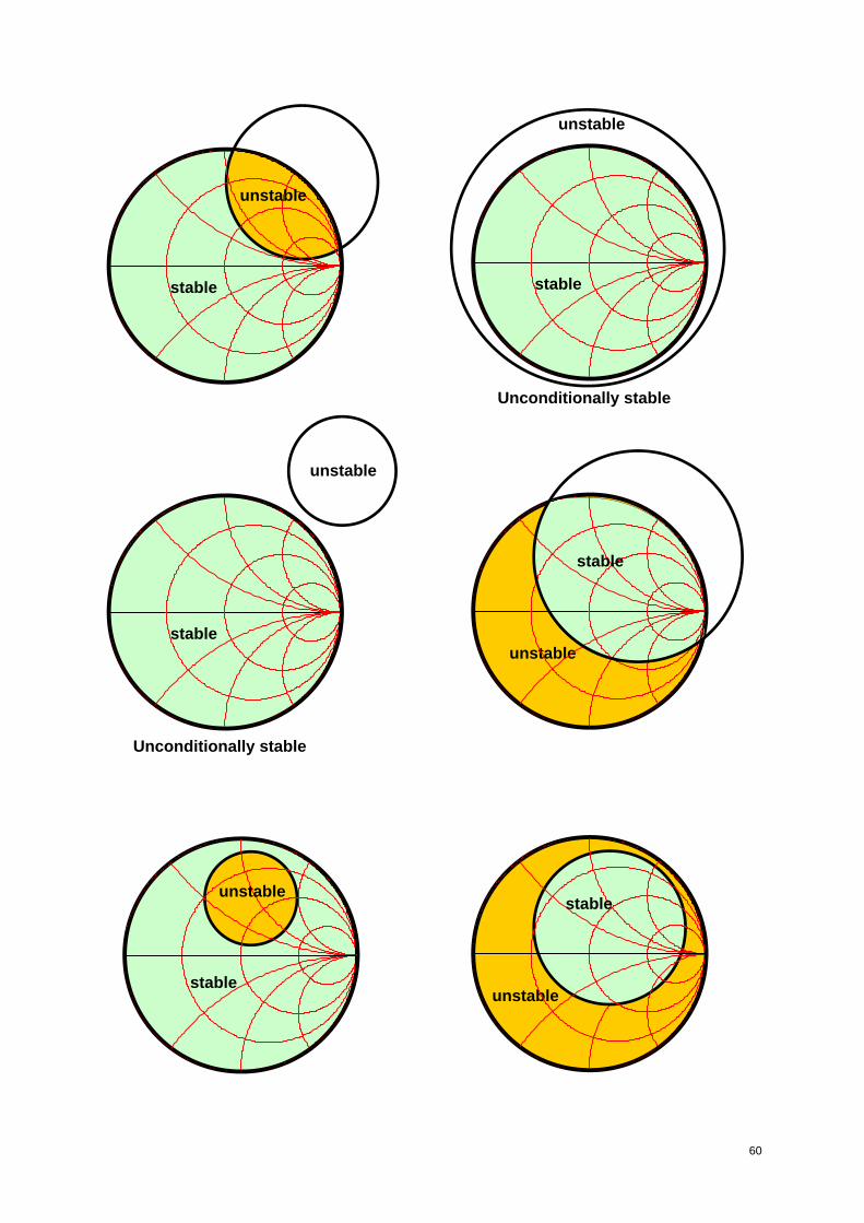
The stable region is inside the stability circle when the center of the Smith-Chart is enclosed, and outside if the center is not enclosed. If the circle lies completely outside the Smith-Chart or completely encloses the Smith-Chart the twoport is unconditionally stable.

Stability circle

|C|

C

60

stable

unstable

stable

unstable

unstable

stable

stable

unstablestable

unstable

stable

unstable

Unconditionally stable

Unconditionally stable

61

Source Stability Circles The Source Stability Circle is the locus of all source impedances for which the magnitude of the output reflection coefficient of the twoport equals 1. The stable region is inside the stability circle when the center of the Smith-Chart is enclosed, and outside if the center is not enclosed. If the circle lies completely outside the Smith-Chart or completely encloses the Smith-Chart the twoport is unconditionally stable.

Load Stability Circles The Load Stability Circle is the locus of all load impedances for which the magnitude of the input reflection coefficient of the twoport equals 1. The stable region is inside the stability circle when the center of the Smith-Chart is enclosed, and outside if the center is not enclosed. If the circle lies completely outside the Smith-Chart or completely encloses the Smith-Chart the twoport is unconditionally stable.

62

Constant Gain Circles

Transducer Power Gain Operating Power Gain Available Power Gain Maximum Available Gain MAG and Maximum Stable Gain MSG Unilateral Transducer Gain Simultaneous Conjugate Match

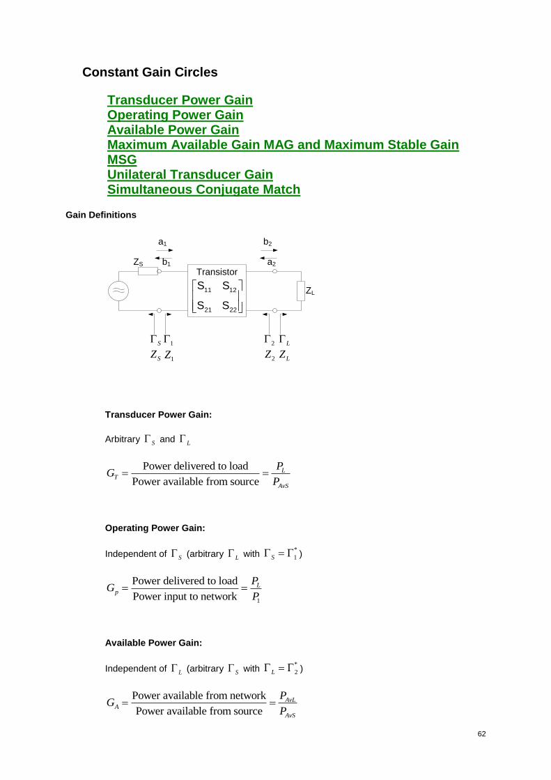
Gain Definitions

ZS

ZL

Transistor

a1

b1

b2

a2

S 1 2 L

LZ2Z1ZSZ

11 12

21 22

S S

S S

Transducer Power Gain:

Arbitrary S and L

Power delivered to load

Power available from source

LT

AvS

PG

P

Operating Power Gain:

Independent of S (arbitrary L with *

1S )

1


Power input to network

Lp

PG

P

Available Power Gain:

Independent of L (arbitrary S with *

2L )

Power available from network


AvLA

AvS

PG

P

63

Transducer Power Gain

Transducer Power Gain

Arbitrary S and L



LT

AvS

PG

P

Z0

Z0

Output

matching

network

Input

matching

network

Transistor

2

Z2

L

ZL

S

ZS

1

Z1

11 12

21 22

S S

S S

2 2 2

21

2

11 22 12 21

1 1

1 1

S L

T

S L S L

SG

S S S S

2 2

2

212 2

1 22

1 1

1 1

S L

T

S L

G SS

12 211 11

221

L

L

S SS

S

or

2 2

2

212 2

11 2

1 1

1 1

S L

T

S L

G SS

12 212 22

111

S

S

S SS

S

64

For : 0 ( 0, 0)G L S LZ Z Z

2

21

2

21 2110log 20log

Zo

Zo

T

T

G S

G dB S S

Operating Power Gain

Operating Power Gain

Independent of S (arbitrary L with *

1S )

Use “Operating Power Gain” for amplifier design with maximum output power, best

efficiency or lowest intermodulation. Choose L for maximum output power, best efficiency

or lowest intermodulation. Match input conjugately to resulting 1 (*

1S ).

12 211 11

221

L

L

S SS

S

1


Power input to network

Lp

PG

P

Z0

Z0

Output

matching

network

Input

matching

network

Transistor

2

Z2

L

ZL

S = 1*

ZS = Z1*

1

Z1

11 12

21 22

S S

S S

65

2 2

21

2 2

1 22

2 2

21

2 2

22 11

2 2

21

2

21122

22

2 2

21

2 2 2 2 *

11 22 22 11

1

1 1

1

1

1

1 11

1

1 2 Re

L

p

L

L

L L

L

LL

L

L

L L

SG

S

S

S S

S

SS

S

S

S S S S

11 22 12 21S S S S

Constant Operating Power Gain circles:

The Operating Power Gain Circle is the locus of all load impedances for constant operating power gain. The input is conjugately matched to the resulting input reflection coefficient.

2 2

12 21 12 21

2 2

22

1 2

1

p p

p

p

K S S g S S gR

g S Radius load plane

*

22 11

2 2

22

*

1

p

p

p

g S SC

g S Center load plane

2

21

Zo

p p

p

T

G Gg

G S Gain reduction for circle

Gp: Desired gain

66

Maximum Available Gain MAG and Maximum Stable Gain MSG

Maximum Available Gain:

max max

221

12

1p T

SMAG G G K K

S ( 1)K

2 2 2

11 22

12 21

11

2

S SK

S S

Maximum Stable Gain:

21

12

SMSG

S 1K

Available Power Gain

Available Power Gain

Independent of L (arbitrary S with *

2L )

Use Available Power Gain for low noise amplifier design. Choose S for lowest noise

figure. Match output conjugately to resulting 2 (*

2L ).

12 212 22

111

S

S

S SS

S

Power available from network


AvLA

AvS

PG

P

67

Z0

Z0

Output

matching

network

Input

matching

network

Transistor

2

Z2

S

ZS

1

Z1

L = 2*

ZL = Z2*

11 12

21 22

S S

S S

2 2

21

2 2

11 2

2 2

21

2 2 2 2 *

22 11 11 22

1

1 1

1

1 2 Re

S

A

S

S

S S

SG

S

S

S S S S

Constant Available Power Gain circles:

The Available Power Gain Circle is the locus of all source impedances for constant available power gain. The output is conjugately matched to the resulting output reflection coefficient.

2 2

12 21 12 21

2 2

11

1 2

1

A A

A

A

K S S g S S gR

g S Radius source plane

*

11 22

2 2

11

*

1

A

A

A

g S SC

g S Center source plane

2

21

Zo

A AA

T

G Gg

G S Gain reduction for circle

GA: Desired gain

68

Unilateral Transducer Gain

Unilateral Transducer Gain

12 1 11 2 220S S S

Use Unilateral Transducer Gain for first approximation of matching network.

Z0

Z0

GLGS

Transistor

S22S11

G0

Input

matching

network

Output

matching

network

LS

2 2

2

212 2

11 22

1 1

1 1

S L

TU

S L

G SS S

TU S o LG G G G

2 2

2

212 2

11 22

1 1

1 1

S L

S o L

S L

G G S GS S

Maximum unilateral gain can be achieved by conjugate match:

11 L 22 and S S S

max 2

11

1

1SG

S

max 2

22

1

1LG

S

max

2

212 2

11 22

1 1

1 1TUG S

S S

„Unilateral Figure of Merit“ U:

12 21 11 22

2 2

11 221 1

S S S SU

S S

69

Error boundaries:

2 2

1 1ˆ

1 1

Teff

TU

GE E E

GU U

2 2

1 110log 10log 10log

1 1

T

TU

G

GU U

Maximum error in dB

max 2 2

1 110log 10log

1 1E dB

U U

On error larger than 1 dB (U>0.1) unilateral approximation is not valid.

Constant unilateral gain circles:

2

11

2

11

1 1

1 ( 1)

SU

SU

SU

g SR

S g Radius source plane

*

11

2

111 ( 1)

SUSU

SU

g SC

S g Center source plane

max

2

111 SSU S

S

Gg G S

G Gain reduction for circle

GS: Desired gain

2

22

2

22

1 1

1 ( 1)

LU

LU

LU

g SR

S g Radius load plane

70

*

22

2

221 ( 1)

LULU

LU

g SC

S g Center load plane

2

22

max

1 LLU L

L

Gg G S

G Gain reduction for circle

GL: Desired gain

Simultaneous Conjugate Match

Simultaneous Conjugate Match

* *

1 2 1S L K

Give maximum gain. Device has to be unconditionally stable 1K .

22

1 1 1*

1

1

2 2 2

1 11 22

*

1 11 22

4

2

1

SCM

B B C

C

B S S

C S S

Source

22

2 2 2*

2

2

2 2 2

2 22 11

*

2 22 11

4

2

1

LCM

B B C

C

B S S

C S S

Load

71

Constant Noise Figure Circles

Noise Figure

2

min 22

4

1 1

n S Sopt

S Sopt

rF F

minF = Minimum noise factor =

min

1010NF

minNF = Minimum noise figure in dB

nr = equivalent normalized noise resistance =

0

nR

Z

Sopt = source reflection coefficient that produces minF

Constant noise circle:

2

2 1

1

i i Sopt

Fi

i

N N

RN

Radius

1

Sopt

Fi

i

CN

Center

2

min 14

ii Sopt

n

F FN

r

iF = desired noise factor (> minF )

72

File format info

Touchstone®

Twoport-Parameter - Files (S-, H-, Z-, Y- and ABCD-Parameter) in Touchstone

® - Format must follow

the rules below: In one line all characters after an exclamation-mark „!“ are comment only. The line terminates

with carriage return and line feed

In front of data there must be a parameter-line: <Frequency unit> <Parameter-designation> <Format> <R n>

: Parameter-line designator

<Frequency unit>: „GHz“, „MHz“, „kHz“ or „Hz“

<Parameter-Designation>: „S“ for S-Parameter „H“ for H-Parameter „Z“ for Z-Parameter „Y“ for Y-Parameter.

<Format>: „MA“: magnitude-angle „DB“: decibel-angle „RI“: real-imaginary

<R n>: n = normalization impedance in Ohm (e.g. R 50)

Data: Each line contains the data for one frequency. The parameters are separated with one space minimum. Data must be in following sequence:

1. Frequency

2. Magnitude, decibel or real part of x11

3. Imaginary part or angle of x11







x = S, H, Z, or Y. Frequencies must be ascending sequence

At the end of the twoport parameters, noise parameters can be added: Each line contains the data for one frequency. The parameters are separated with one space minimum. Data must be in following sequence:

1. Frequency

2. Nfmin Minimum Noise Figure in dB

73

3. Magnitude of reflection coefficient for NFmin (Gamma_opt)

4. Angle of reflection coefficient for NFmin (Gamma_opt) in degree

5. Normalized equivalent noise resistor

The lowest noise parameter frequency must be less or equal to the highest S-Parameter frequency.

Example: ! SIEMENS Small Signal Semiconductors ! CF750 ! GaAs Microwave Monolithic Integrated Circuit in SOT143 ! VDGND = 3.8 V ID = 2 mA ! Common Source S-Parameters: April 1992 ! Parameters valid for V D-GND between 3.0 and 5.0 VDC ! for Id=1.6mA MAG[S21] is abt. 10% lower ! for Id=2.8mA MAG[S21] is abt. 20% higher ! >>>>>> Source bypass capacitor must be low inductance!! # GHz S MA R 50 ! f S11 S21 S12 S22 ! GHz MAG ANG MAG ANG MAG ANG MAG ANG 0.010 0.9700 -1.0 1.780 179.0 0.0020 89.0 0.9800 -1.0 0.100 0.9700 -3.0 1.780 175.0 0.0080 84.0 0.9800 -2.0 0.250 0.9600 -8.0 1.760 169.0 0.0150 78.0 0.9700 -6.0 0.500 0.9400 -16.0 1.730 155.0 0.0270 75.0 0.9500 -11.0 0.750 0.9100 -26.0 1.700 141.0 0.0390 71.0 0.9300 -16.0 1.000 0.8700 -34.0 1.680 127.0 0.0460 64.0 0.9100 -22.0 1.250 0.8300 -42.0 1.650 118.0 0.0540 62.0 0.8900 -26.0 1.500 0.7800 -49.0 1.620 108.0 0.0610 57.0 0.8800 -30.0 1.750 0.7200 -57.0 1.590 95.0 0.0660 55.0 0.8700 -34.0 2.000 0.6600 -65.0 1.540 82.0 0.0690 52.0 0.8600 -38.0 2.250 0.6100 -73.0 1.510 71.0 0.0710 54.0 0.8500 -43.0 2.500 0.5600 -81.0 1.470 60.0 0.0730 60.0 0.8400 -48.0 2.750 0.5200 -87.0 1.450 52.0 0.0740 63.0 0.8300 -52.0 3.000 0.4900 -93.0 1.420 45.0 0.0750 66.0 0.8200 -56.0 ! ! NOISE ! f Fmin Gammaopt rn/50 ! GHz dB MAG ANG - 0.900 1.60 0.63 26 0.98 1.800 1.90 0.52 51 0.72 ! ! SIEMENS AG Semiconductor Group, Munich

Touchstone

®: Copyright by Keysight/Agilent/EEsof

74

CITI

(Text adopted from Agilent) Overview CITIfile is a standardized data format that is used for exchanging data between different computers and instruments. CITIfile stands for Common Instrumentation Transfer and Interchange file format. CITIfile defines how the data inside an ASCII package is formatted. Since it is not tied to any particular disk or transfer format, it can be used with any operating system, such as DOS or UNIX, with any disk format, such as DOS or HFS, or with any transfer mechanism, such as by disk, LAN, or GPIB. By careful implementation of the standard, instruments and software packages using CITIfile are able to load and work with data created on another instrument or computer. It is possible, for example, for a network analyzer to directly load and display data measured on a scalar analyzer, or for a software package running on a computer to read data measured on the network analyzer. Data Formats CITIfile uses the ASCII text format. The ASCII format is accepted by most text editors. This allows files to be created, examined, and edited easily, making CITIfile easy to test and debug.

CITIfile Definitions This section defines: package, header, data array, and keyword. Package A typical CITIfile package is divided into two parts:

The header is made up of keywords and setup information.

The data usually consists of one or more arrays of data. The following example shows the basic structure of a CITIfile package:

When stored in a file there may be more than one CITIfile package. With the Agilent 8510 network analyzer, for example, storing a memory all will save all eight of the memories held in the instrument. This results in a single file that contains eight CITIfile packages. Header The header section contains information about the data that will follow. It may also include information about the setup of the instrument that measured the data. The CITIfile header shown in the first example has the minimum of information necessary; no instrument setup information was included. Data Array An array is numeric data that is arranged with one data element per line. A CITIfile package may contain more than one array of data. Arrays of data start after the BEGIN keyword, and the END keyword follows the last data element in an array. A CITIfile package does not necessarily need to include data arrays. For instance, CITIfile could be used to store the current state of an instrument. In that case the keywords VAR, BEGIN, and END would not be required. When accessing arrays via the DAC (DataAccessComponent), the simulator requires array elements to be listed completely and in order. Example: S[1,1], S[1,2], S[2,1], S[2,2] Keywords Keywords are always the first word on a new line. They are always one continuous word without embedded spaces.

75

CITIfile Example 2-Port S-Parameter Data File This example shows how a CITIfile can store 2-port S-parameter data. The independent variable name FREQ has two values located in the VAR_LIST_BEGIN section. The four DATA name definitions indicate there are four data arrays in the CITIfile package located in the BEGIN...END sections. The data must be in the correct order to ensure values are assigned to the intended ports. The order in this example results in data assigned to the ports as shown in the table that follows:

CITIFILE A.01.00 NAME BAF1 VAR FREQ MAG 2 DATA S[1,1] MAGANGLE DATA S[1,2] MAGANGLE DATA S[2,1] MAGANGLE DATA S[2,2] MAGANGLE VAR_LIST_BEGIN 1E9 2E9 VAR_LIST_END BEGIN 0.1, 2 0.2, 3 END BEGIN 0.3, 4 0.4, 5 END BEGIN 0.5, 6 0.6, 7 END BEGIN 0.7, 8 0.8, 9 END

DATA FREQ = 1E9 FREQ = 2E9 s[1,1] s[0.1,2] s[0.2,3] s[1,2] s[0.3,4] s[0.4,5] s[2,1] s[0.5,6] s[0.6,7] s[2,2] s[0.7,8] s[0.8,9] For more information see Keysight/Agilent documentation.

76

EZNEC

EZNEC is a very powerful antenna simulation tool. It creates a datafile “Lastz.txt”. The Lastz.txt file is created when a Frequency Sweep or SWR sweep is run. It contains, in comma-delimited ASCII format, the impedance and SWR at each source and frequency. It remains in the EZNEC program directory after the program ends and can be used for other purposes if desired. Text headers in the first line identify the field contents. Freq MHz Frequency in MHz Src# Number of source R Real part of impedance X Imaginary part of impedance SWR (50 ohms) VSWR referenced to 50 Ohms SWR (alt Z0) VSWR referenced to other specified resistance Example: "EZNEC+ ver. 5.0" "Vert13m h=2,5m 4xRad6m Hut4x7m","10.09.2008 12:48:36" "Alt Z0: ",75 "Freq MHz","Src #","R","X","SWR (50 ohms)","SWR (alt. Z0)" 3.4,1,30.0344,-104.4704,9.427082,7.611355 3.45,1,31.09572,-87.45639,7.006533,5.937705 3.5,1,32.19752,-70.44454,5.082611,4.596093 3.55,1,33.35558,-53.0484,3.573638,3.53528 3.6,1,34.53947,-35.95722,2.484591,2.770061 3.65,1,35.77891,-18.79243,1.733638,2.262968 3.7,1,37.08047,-1.231948,1.350235,2.02335 3.75,1,38.42399,16.13573,1.567183,2.071931 3.8,1,39.82835,33.66065,2.157393,2.371814 3.85,1,41.2804,51.10541,2.964938,2.861347 3.9,1,42.81051,68.93056,3.993486,3.518317 For more information see EZNEC documentation.

77

References

[1] Medley, Max W.: Microwave and RF Circuits: Analysis, Synthesis and Design. Norwood: Artech House, Inc., 1993. ISBN 0-89006-546-2

[2] Gonzalez, Guillermo: Microwave transistor amplifiers. Englewood Cliffs: Prentice-Hall, Inc.,

1984. ISBN 0-13-581646-7 [3] Vendelin, George David: Microwave circuit design using linear and nonlinear techniques.

New York: John Wiley & Sons, 1990. ISBN 0-471-60276-0 [4] Dellsperger, Fritz: Vorlesung Hochfrequenztechnik, Kapitel "Leitungen" (Lecture: High

Frequency Engineering, Chapter "Lines") 1989-2005, Bern University of Applied Sciences

[5] Dellsperger, Fritz: Vorlesung "Verstärker-Entwurf mit S-Parameter" (Lecture: Amplifier

Design with S-Parameter) 1997-2005, Bern University of Applied Sciences

[6] M.L. Edwards/J.H. Sinsky: A new criterion for linear 2-port stability using geometrically

derived parameters IEEE Transaction on MTT, Vol. 40, No. 12, pp. 2303-2311, Dec. 1992

[7] Pieper, Ron; Dellsperger, Fritz: Personal Computer Assisted Tutorial for Smith-Charts

IEEE Proceedings of the 33rd

Southeastern Symposium on System Theory, pp. 139-143, March 2001

[8] Dellsperger, Fritz; Kaufmann, Alfred: Vorlesung "Telekom-Elektronik" (Lecture: Telecom electronics, circuit design) 2006-2012, Bern University of Applied Sciences

[9] Keysight/Agilent/EEsof: Advanced Design System, ADS 2009, Documentation www.keysight.com

[10] Lewallen, Roy, W7EL: EZNEC Antenna Software, Documentation www.eznec.com

http://www.keysight.com/

http://www.keysight.com/

http://www.eznec.com/

78

License, Demoversion and Contact The unlicensed Demoversion allows 5 elements and 5 datapoints only. Save project and save netlist are disabled. If you are interested in a licensed version with full capabilities send an e-mail to [email protected] Commercial licenses are priced to US$ 120 Licenses for universities, students and Ham’s with callsign are priced to US$ 80 Demoversion and additional documents related to the Smith-Chart can be downloaded at www.fritz.dellsperger.net

mailto:[email protected]


79

It’s a long way to a perfect software... If this ever exists... While using our Smith software you may find bugs or new features to implement. Send me a mail. For next version we will fix the bugs and maybe put a few new ones. We will also think about new features... We’re working hard... Prof. Fritz Dellsperger Dipl. Ing. Michel Baud October 2016 May 2010 January 2010 October 2009 September 2005 November 2004 Former team members at Bern University of Applied Sciences Engineering and Information Technology Division of Electrical- and Communication Technology Jürg Tschirren Roger Wetzel Martin Aebersold Stephan Roethlisberger April 2004 March 2004 July 2002 July 2000 February 1998 August 1995

80

History Version 4.0 to Version 4.1, January 2018

Fixed bug in labels of circles (VSWR, Q) Solved Problems with multiple datapoints and editing or tuning serial line Solved Problems with multiple datapoints, datapoint sweep and tuning serial line length Corrected text for Operating Power Gain Circles in circle window Fixed bug with input for “number of points” in frequency sweep Corrected CITI file load problems in S-Plot Corrected S21 and S12 swapping in s2p file from “Export > CITI-to S” in S-Plot Fixed different labels and minor bugs in “Smith” and “S-Plot”

Version 3.01 to Version 4.0, October 2016

Added Tuning Cockpit to tune element values with sliders Fixed bugs in element definitions, frequency sweeps and other subjects Solved problems with Decimal Symbol in window settings Corrected file load problems in S-Plot Minor changes in menue and dialog boxes

Version 3.01 to Version 3.10, May 2010

Added Frequency and Datapoint Sweep Serial transmission line with loss (attenuation) Export datapoint and circle info to ASCII-file for post-processing in spreadsheets or math software Linear or logarithmic frequency axis in S-Plot graphs Cursor readout in S-Plot graphs Minor changes in toolboxes and settings

Version 3.0 to Version 3.01, January 2010

Fixed problem with key-files including “Umlauts” and other vowel mutations Allow delete of manually defined VSWR-circles Solved problems with gain-, noise- and stability-circle dialogbox Automatic update of values in schematic on selecting active datapoint and insert circuit elements Fixed bug for line length units in schematic Last input of Er on line elements will be default value for next line insertion Replaced “Ohm” with greek in some dialogboxes Removed unused checkbuttons in window “Datapoints” Correct frequency assignment from datapoints to circuit elements

Version 2.03 to Version 3.0, October 2009

Complete redesign

Version 2.02 to Version 2.03, September 2005

Version 2.01 to Version 2.02, November 2004

Version 2.00 to Version 2.01, April 2004

Version 1.92 to Version 2.0, March 2004

Version 1.91 to Version 1.92, July 2002

Version 1.90 to Version 1.91, July 2000

Version 1.82 to Version 1.90, June 2000

Version 1.71 to Version 1.82, February 1998

Version 1.0, August 1995

Help for Smith V4 - fritz.dellsperger.net Smith/Help V4.1 -print.pdf · Smith-Chart Activate...

Documents

Transcript of Help for Smith V4 - fritz.dellsperger.net Smith/Help V4.1 -print.pdf · Smith-Chart Activate...