HE UNIVERSITY OF QUEENSLAND

Faculty of Engineering, Architecture and Information Technology

THE UNIVERSITY OF QUEENSLAND

Characterising the Rheology of Fermented Dairy Products During Filling

Student Name: Hera, WILLIAMSON Course Code: ENGG7290 Supervisor: Jason Stokes, Professor and Director of Research, School of Chemical

Engineering Submission date: 9 June 2019

iii

Executive Summary One of the current difficulties with processing and modelling fermented dairy products is their

complex behaviour, which is a result of the gel structure created during fermentation. For the

purposes of Tetra Pak, the simplest rheological models (Newtonian and Power Law) are not

sufficient for fluid modelling or as indicators of behaviour in operations such as filling.

This study aimed to improve the characterisation of the rheological behaviour of fermented dairy

products by applying a variety of existing and developed measurement techniques. Three products

(Skånemejerier Vaniljyoghurt, Skånemejerier Naturell Lättyoghurt and Arla Långfil) were

characterised using these techniques. The results were then correlated to issues observed during

testing in a pilot scale filling rig. The rheological models were to be validated by measuring the

thickness profile of the products on a metal plate with a laser scanner (‘pulled plate’ rig), and then comparing the results to computational fluid dynamics (CFD) simulations of the same scenarios.

This study demonstrated that it is possible to measure the observable differences in filling behaviour

between the products with the chosen measurement- and analysis methods, and existing equipment.

The pulled plate rig testing demonstrated that it is possible to record surface- and thickness profiles

of the products with a laser scanner. While the results were not compared to the CFD simulations

due to complications during the modelling, the existence of yield stress was confirmed.

The fill rig testing demonstrated that it is possible to quantify issues in automatic filling machines,

such as dripping and splashing. The subsequent statistical analyses (Pearson Correlation

Coefficients and Partial Least Square) suggests that the frequency of these issues can be predicted

using measurable rheological parameters. Based on the results from the characterisation and fill rig

tests, it was concluded that the variables A, b and nε could be experimentally determined and then

correlated to the flow behaviour of the studied products.

From the investigations presented in this study, the following measurement- and analysis methods

are suggested to characterise the studied products:

• Linear stress ramp and Tangent analysis method for yield stress determination

• Shear rate sweep and Herschel-Bulkley curve fitting (including yield stress) for A and b

determination

• Pulled plate validation method for comparison with future CFD modelling

• Pilot scale fill rig testing for identification and quantification of issues during automatic

filling

iv

Acknowledgements I would like to thank my supervisors, Jason Stokes, Professor and Director of Research, School of

Chemical Engineering (The University of Queensland) and Andreas Håkansson, Senior Lecturer at

the Department of Food Technology (Lund University), Andreas Håkansson, for support

throughout the course of the project and valuable feedback along the way.

This work would not have been possible without the assistance and experience of my industry

supervisors, Fredrik Innings and Jenny Jonsson, and several experts within Tetra Pak’s Packaging and Processing Systems departments. These experts were Dragana Arlov, Thomas Wiese, Lars-

Göran Larsson and Robert Dring, who all provided insight into the issues this project hoped to

address and the broader scope of this project within Tetra Pak’s operations. They also gave assistance in organising and conducting testing when this was conducted at Tetra Pak’s Product Development

Centre and Packaging Laboratory.

This work was completed in close collaboration with Rebecka Ostréus, a fellow Master of Science

in Engineering student at Lunds Tekniska Högskola, as we worked together on this joint study

conducted on behalf of Tetra Pak. Rebecka contributed to the development and execution of the

characterisation experiments presented in this report and was equally involved in the analysis of these

results.

I would like to thank RISE, Department of Agrifood and Bioscience, for their interest in our joint

project and assistance during the measurements performed at their rheology lab. Special thanks go

to Johanna Andersson, Emma Bragd and Waqas Quazi. I would finally like to thank Anders Åkesjö

at Chalmers University of Technology, for his assistance with the set-up and use of the laser profiler.

v

Table of contents Executive Summary iii

Acknowledgements iv

Table of contents v

List of Tables viii

List of Figures x

List of Abbreviations and Symbols xiii

1 Introduction 1

1.1 Background and motivation 1

1.2 Objectives 2

1.3 Research questions 3

1.4 Scope and limitations 3

1.5 Key deliverables 4

2 Theoretical framework 5

2.1 Rheological models 5

2.1.1 Shear-rate dependent models 5

2.1.2 Yield stress models 6

2.1.3 Time-dependent models 6

2.1.4 Extensional viscosity models 7

2.2 Shear rheological parameter determination 8

2.2.1 Power Law constants 9

2.2.2 Yield stress 10

2.2.3 Zero-shear viscosity 11

2.2.4 Viscosity at infinite shear rate 12

2.2.5 Relaxation time 13

2.2.6 Thixotropy 14

2.3 Extensional rheological parameter determination 14

2.3.1 Extensional viscosity 14

3 Methodology 16

3.1 Sample preparation and handling 16

3.2 Rotational rheometer 19

3.2.1 Materials 19

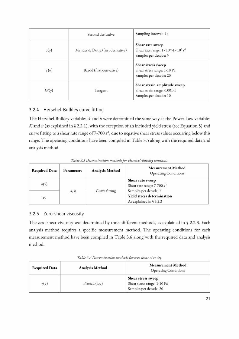
3.2.2 Power Law curve fitting 20


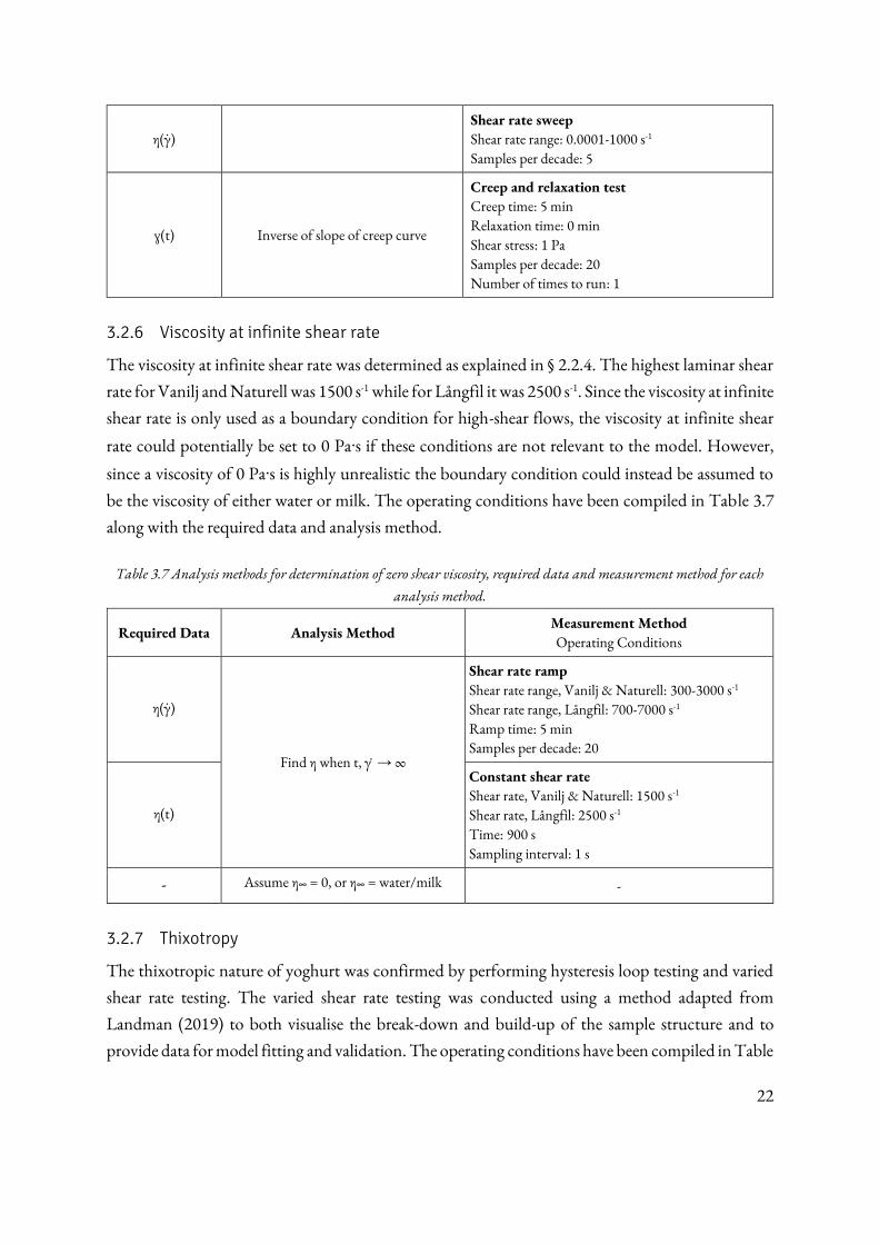
3.2.4 Herschel-Bulkley curve fitting 21


vi


3.2.7 Thixotropy 22

3.3 Extensional rheometer 24

3.3.1 Materials 24

3.3.2 Extensional viscosity 25

3.4 Pulled plate rig and laser profiler 26

3.4.1 Materials 26

3.4.2 Operating conditions 26

3.4.3 Data treatment 28

3.5 Stand-alone filling rig 28

3.5.1 Materials 29

3.5.2 Operating conditions 29

3.5.3 Quantification and statistical analyses 30

4 Results 31

4.1 Rotational rheometer 31

4.1.1 Power Law curve fitting 31


4.1.3 Herschel-Bulkley curve fitting 33



4.1.6 Thixotropy 36

4.2 Extensional rheometer 38

4.2.1 Extensional K and n 38

4.2.2 Trouton ratio 39

4.3 Pulled-plate rig and laser profiler 40

4.3.1 Profile thickness 40

4.3.2 Comparison with rheological models and CFD 44

4.4 Stand-alone Filling Rig 45

4.4.1 Observed behaviours 45

4.4.2 Viscosity monitoring 48

4.4.3 PLS statistical analysis 49

5 Discussion 51

5.1 Characterisation methods and parameters 51

5.2 Comparison of behaviour indicators 53

5.3 Evaluation of validation methods 54

5.3.1 Pulled plate method 54

vii

5.3.2 Filling rig method 55

5.4 Experimental uncertainty and error 56

5.4.1 Limitations of methodology 56

5.4.2 Uncertainty and reliability 57

5.4.3 Error and validity 59

6 Conclusion and Recommendations 60

6.1 Future work 61

7 References 62

8 Appendices 65

8.1 Additional characterisation results and methodologies 65

8.1.1 Measurement method sequences (Kinexus) 65

8.1.2 Kinexus rheometer methodology 67

8.1.3 Constant characteristic relaxation time 68

8.1.4 HCF rheometer methodology 70

8.1.5 Comparison of product stability 72

8.2 Additional validation results and methodologies 73

8.2.1 Pulled plate rig and laser profiler methodology 73

8.2.2 Stand-alone fill rig methodology 74

8.2.3 Fill rig quantification and statistical analysis 75

8.3 Equipment ranges and resolutions 78

8.4 Project timeline 79

8.5 Project risks 80

8.5.1 Risk matrix 80

8.5.2 Physical risks 80

8.5.3 Planning risks 81

8.6 SEAL analyses 82

8.6.1 SEAL Analysis: Organising a mid-term evaluation meeting 82

8.6.2 SEAL Analysis: Conducting and completing pilot-scale testing 83

8.6.3 SEAL Analysis: Thesis defense at Lund University 84

viii

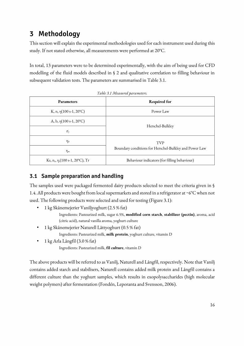
List of Tables Table 3.1 Measured parameters. ......................................................................................................... 16

Table 3.2 Established sample homogenisation methods, stabilisation times and resting times. ...... 18

Table 3.3 Determination methods for Power Law constants. ........................................................... 20

Table 3.4 Determination methods for yield stress.............................................................................. 20

Table 3.5 Determination methods for Herschel-Bulkley constants. ................................................. 21

Table 3.6 Determination methods for zero shear viscosity. ............................................................... 21

Table 3.7 Analysis methods for determination of zero shear viscosity, required data and

measurement method for each analysis method. ................................................................................ 22

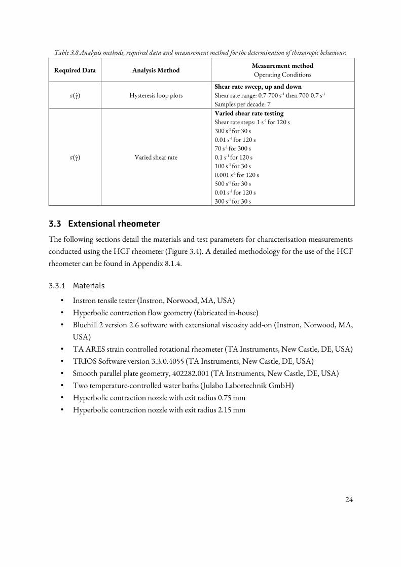
Table 3.8 Analysis methods, required data and measurement method for the determination of

thixotropic behaviour. ......................................................................................................................... 24

Table 3.9 Required data, analysis method, measurement method and operating conditions for Kε

and nε determination. ........................................................................................................................... 25

Table 3.10 Descriptions of the operating conditions used during fill rig testing. ............................ 29

Table 4.1 Methods and n, K and R2 values of Vanilj, Naturell and Långfil..................................... 32

Table 4.2 Yield stress results from Tangent and Bayod methods. ..................................................... 33

Table 4.3 Methods and A, b and R2 values of Vanilj, Naturell and Långfil, using the Tangent and

Bayod methods for σy determination. ................................................................................................. 34

Table 4.4 Method used, and the η0 of Vanilj, Naturell and Långfil. ................................................. 35

Table 4.5 Results of η∞ determination methods for Vanilj, Naturell and Långfil. .......................... 36

Table 4.6 Method used, and the Kε, nε and R2 values of Vanilj, Naturell and Långfil. .................... 39

Table 4.7 Shear viscosities (η) and extensional viscosities (ηε) at an extension rate at 1, 10 and 100,

and the calculated Trouton ratio (Tr). ............................................................................................... 39

Table 4.8 Profile thickness and stress balance results from cycles 2-5 over the region 70-95 mm. .. 41

Table 4.9 Frequency of the different behaviours for each setting and product. ............................... 48

Table 4.10 Viscosity at γ ̇ = 100 s-1 before and after processing, according to Tetra Pak’s method. . 49

Table 8.1 Yield stress results from all tested methods. ....................................................................... 65

Table 8.2 Parameters required for CFD model fitting and modelling. ............................................. 65

Table 8.3 Summary of investigated sequences available for the Malvern Kinexus rheometer. ........ 66

Table 8.4 Required data, analysis methods and operating conditions for determining the

characteristic relaxation time ............................................................................................................... 69

Table 8.5 Method used, and the θ value of Vanilj, Naturell and Långfil. ......................................... 70

Table 8.6 Quantified issues during filling. .......................................................................................... 75

Table 8.7 Results of correlation coefficients. Cells highlighted in green, yellow and red indicate

correlation coefficients of >|0.99|, >|0.95| and >|0.90|, respectively. ............................................... 77

ix

Table 8.8 Summary of rheological values collected before and after processing, during the fill rig

tests, according to the Tetra Pak method. One replicate was taken per product and setting. .......... 77

Table 8.9 Malvern Kinexus Pro+ equipment specifications (Reproduced from: Malvern, 2017). . 78

Table 8.10 Matrix of risk levels............................................................................................................ 80

Table 8.11 Physical risk assessment. .................................................................................................... 80

Table 8.12 Project planning risk assessment. ...................................................................................... 81

x

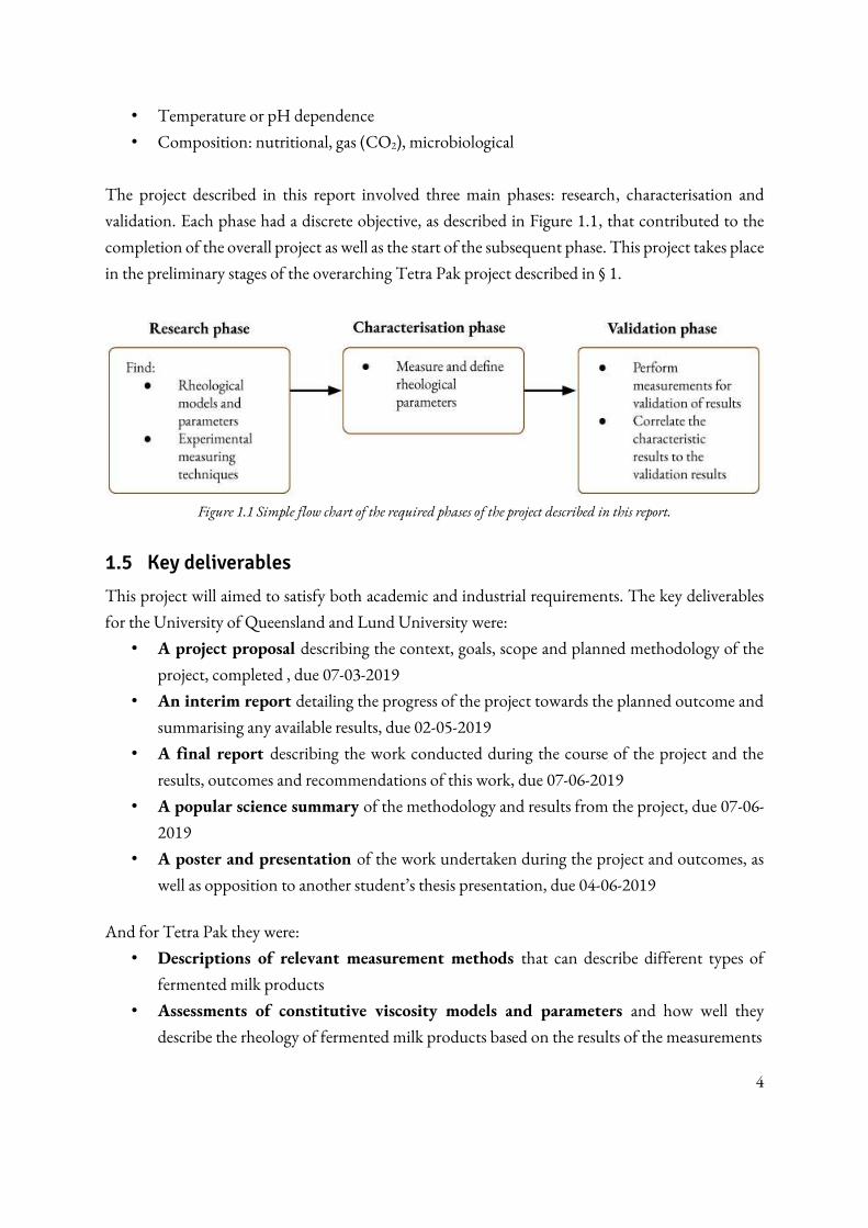
List of Figures Figure 1.1 Simple flow chart of the required phases of the project described in this report. ............. 4

Figure 2.1 Schematic of the cup-and-bob geometry in a rotational rheometer (reproduced from:

Radhakrishnan, van Lier and Clemens, 2018). .................................................................................... 8

Figure 2.2 Graph of potential test regimes. Viscometric measurements conducted in a) step test, b)

ramp testing and c) sweep testing, where either shear rate or shear stress is the controlled variable.

Oscillatory measurements conducted in d) frequency sweep or e) amplitude sweep tests, where the

varied amplitude can be shear stress or shear strain (adapted from: Macosko, 1994; Anton Paar

GmbH, 2019)......................................................................................................................................... 9

Figure 2.3 Example of K and n determination from shear rate sweep data (adapted from: Morrison,

2004). ...................................................................................................................................................... 9

Figure 2.4 Example of σy determination from shear stress ramp data using a) the Maximum viscosity

method and b) the Tangent method c) the Second derivative method. ............................................ 10

Figure 2.5 Example of σy determination from a) stress amplitude sweep data using three different

analysis methods (adapted from: Malvern Instruments, 2012) and b) shear rate or shear stress sweep

tests using the Mendes and Dutra (2004) or Bayod (2007) methods. ............................................... 11

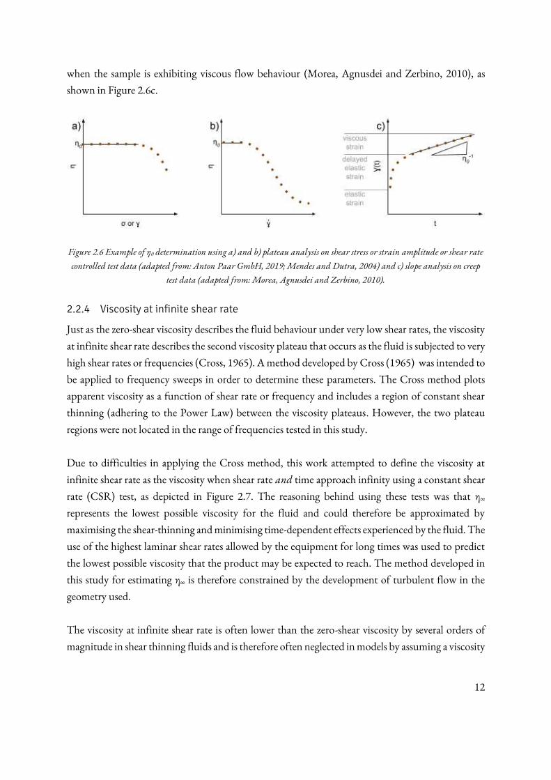
Figure 2.6 Example of η0 determination using a) and b) plateau analysis on shear stress or strain

amplitude or shear rate controlled test data (adapted from: Anton Paar GmbH, 2019; Mendes and

Dutra, 2004) and c) slope analysis on creep test data (adapted from: Morea, Agnusdei and Zerbino,

2010). .................................................................................................................................................... 12

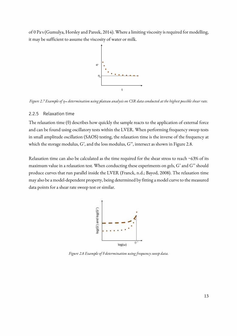
Figure 2.7 Example of η∞ determination using plateau analysis on CSR data conducted at the highest

possible shear rate. ................................................................................................................................ 13

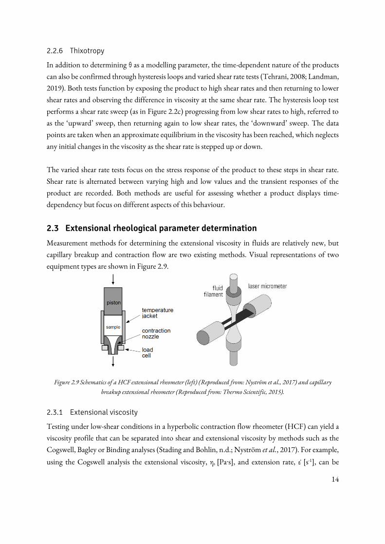
Figure 2.8 Example of θ determination using frequency sweep data. ............................................... 13

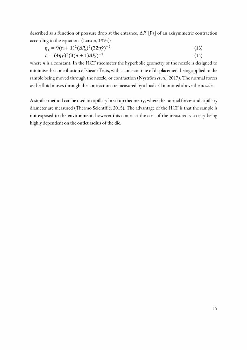
Figure 2.9 Schematics of a HCF extensional rheometer (left) (Reproduced from: Nyström et al.,

2017) and capillary breakup extensional rheometer (Reproduced from: Thermo Scientific, 2015).

.............................................................................................................................................................. 14

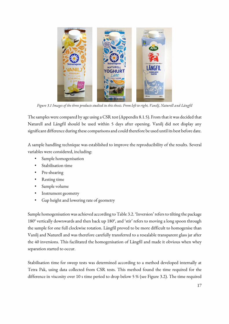
Figure 3.1 Images of the three products studied in this thesis. From left to right, Vanilj, Naturell and

Långfil .................................................................................................................................................. 17

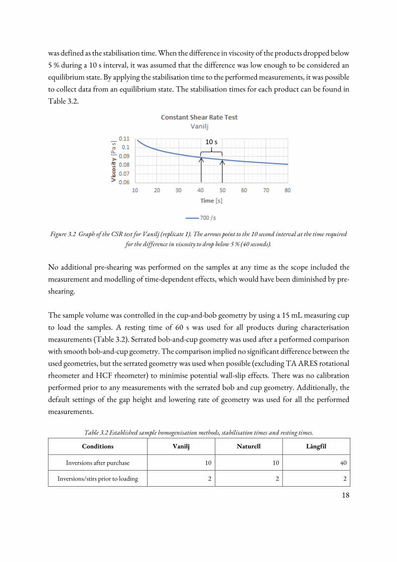
Figure 3.2 Graph of the CSR test for Vanilj (replicate 1). The arrows point to the 10 second interval

at the time required for the difference in viscosity to drop below 5 % (40 seconds). ........................ 18

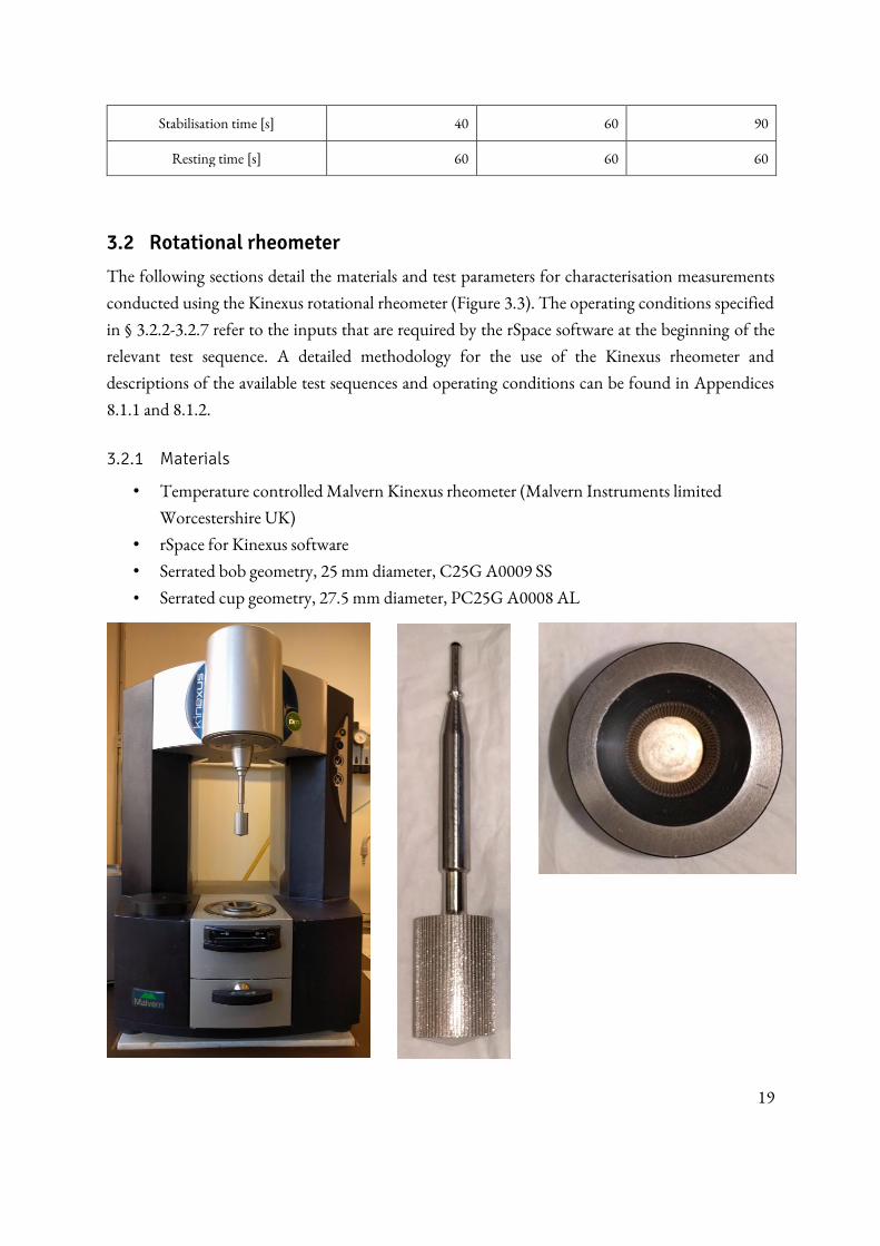
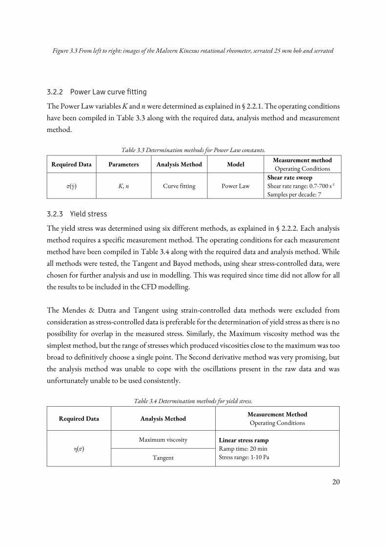
Figure 3.3 From left to right: images of the Malvern Kinexus rotational rheometer, serrated 25 mm

bob and serrated ................................................................................................................................... 20

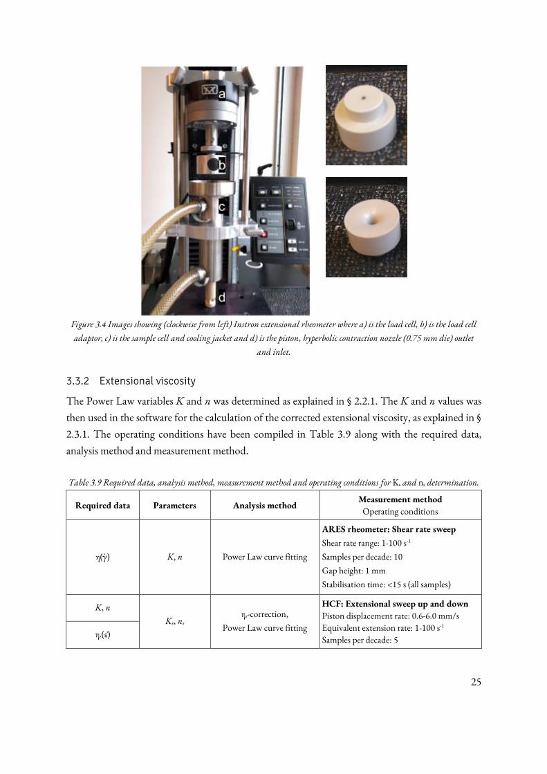
Figure 3.4 Images showing (clockwise from left) Instron extensional rheometer where a) is the load

cell, b) is the load cell adaptor, c) is the sample cell and cooling jacket and d) is the piston, hyperbolic

contraction nozzle (0.75 mm die) outlet and inlet. ............................................................................ 25

xi

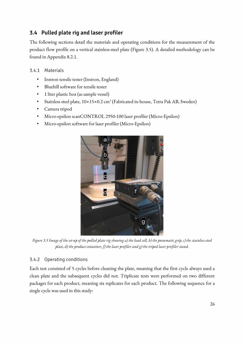
Figure 3.5 Image of the set-up of the pulled plate rig showing a) the load cell, b) the pneumatic grip,

c) the stainless-steel plate, d) the product container, f) the laser profiler and g) the tripod laser profiler

stand. .................................................................................................................................................... 26

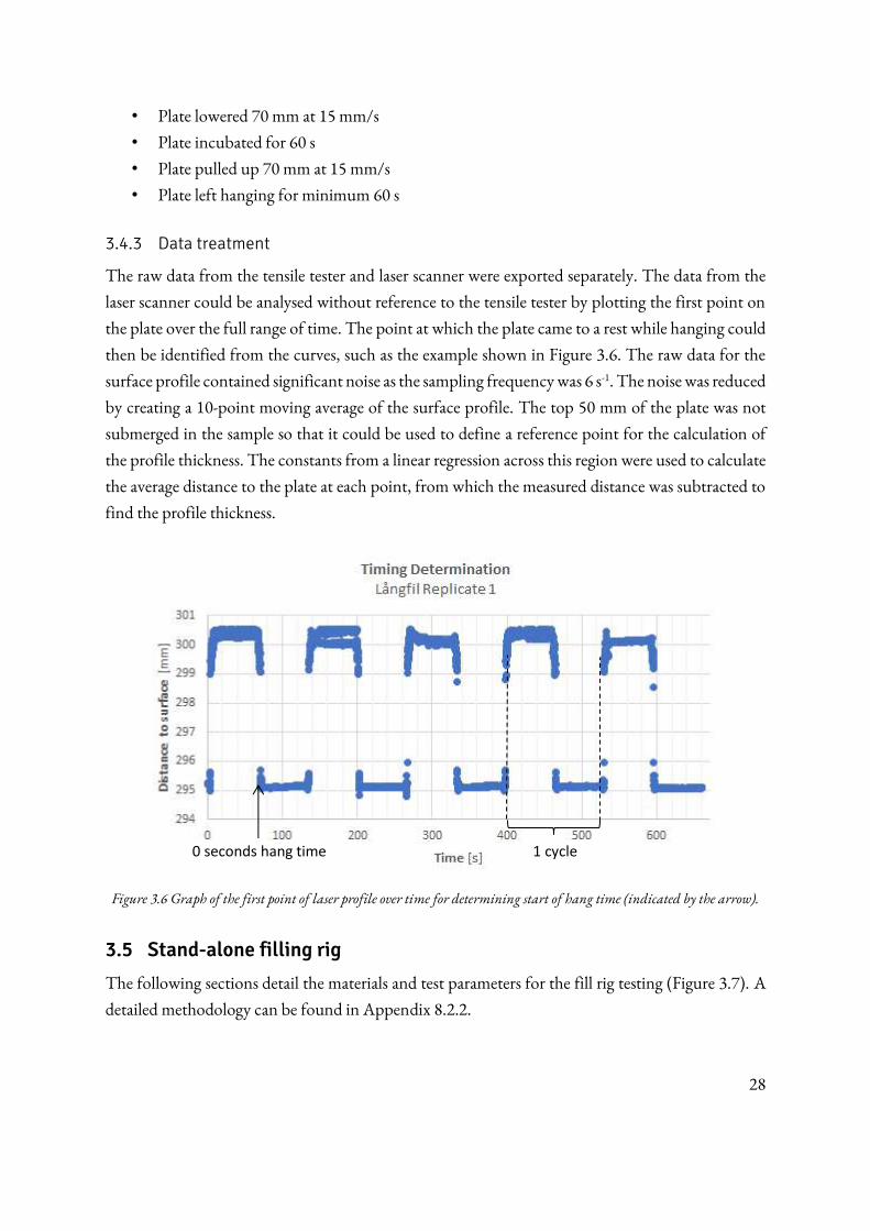
Figure 3.6 Graph of the first point of laser profile over time for determining start of hang time

(indicated by the arrow). ..................................................................................................................... 28

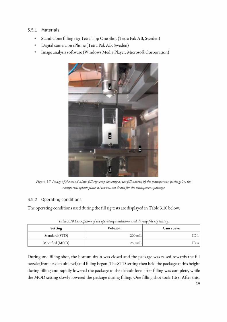
Figure 3.7 Image of the stand-alone fill rig setup showing a) the fill nozzle, b) the transparent

‘package’, c) the transparent splash plate, d) the bottom drain for the transparent package............ 29

Figure 4.1 Graph of the data of replicates one from the shear rate sweep test using the bob-and-cup

geometry and Kinexus rheometer. ...................................................................................................... 31

Figure 4.2 Graphs of the Tangent method for Vanilj, Naturell and Långfil (first replicate). .......... 32

Figure 4.3 Graph of the Bayod method (first derivative method) for one replicate (given within

brackets) of each sample. ..................................................................................................................... 33

Figure 4.4 Graphs of the shear rate sweep (left), shear stress sweep (middle) and creep test methods

(right) for zero-shear viscosity determination. .................................................................................... 34

Figure 4.5 Graph of the constant shear rate tests. Vanilj and Naturell at a shear rate of 1500 s-1 and

Långfil at 2500 s-1. ................................................................................................................................ 36

Figure 4.6 Graph of one replicate (number in brackets) for each product for the single hysteresis loop

tests, with spline for visualisation. Upper line is the upward sweep, lower line is the downward sweep.

.............................................................................................................................................................. 37

Figure 4.7 Graph of the varied shear stress as a function of varying shear rate for all products. ...... 37

Figure 4.8 Graph of the extension rate sweep tests using the 0.75 mm die and equations for the lines

of best fit for one replicate of each sample. ......................................................................................... 38

Figure 4.9 Images comparing the uniformity of the adhered layer in the first cycle (left) and fifth

cycle (right) for Vanilj, with the submersion height marked by a dashed red line. ........................... 40

Figure 4.10 Graphs of flow profile along a clean plate (left) and a re-used plate (right) for replicate 1

of Vanilj. ............................................................................................................................................... 41


of Naturell. ........................................................................................................................................... 42


of Långfil. ............................................................................................................................................. 43

Figure 4.13 Graph of the average flow profiles for runs 2-5 at a hang time of 0 seconds of each sample.

.............................................................................................................................................................. 43

Figure 4.14 Graphs of the simulated flow profile at different points in time (5, 6, 7, 8, 9, 10 s) for the

Power Law model of Vanilj (left) and Långfil (right). Reproduced with permission from Jönsson

(2019). .................................................................................................................................................. 44

xii

Figure 4.15 Graphs of the simulated flow profile at different points in time (5, 6, 7, 8, 9, 10 s) for the

Herschel-Bulkley model of Vanilj (left) TVP model of Vanilj (right). Reproduced with permission

from Jönsson (2019). ........................................................................................................................... 45

Figure 4.16 Image sequence showing a ‘splashing’ event forming a streak and a large droplet. ....... 46

Figure 4.17 Images showing droplets on the fill nozzle (left) and transparent plate (middle), and

droplets and streaks on the package interior (right). .......................................................................... 46

Figure 4.18 Image sequence showing a ‘dripping’ event forming a single drip. ............................... 47

Figure 4.19 Image sequence showing a ‘filamentation’ event. ........................................................... 47

Figure 4.20 W*Q biplot visualising the results of the PLS analysis. .................................................. 50

Figure 5.1 Graph of viscosity as calculated from the Power Law and Herschel-Bulkley constants

determined in § 4.1, as implemented in CFD with the zero-shear viscosities from the three

determination methods superimposed. The range reflects the largest for the experimental shear rate

sweeps (1 ×10-4 - 1000 s-1). ................................................................................................................... 52

Figure 5.2 Graph of the relative uncertainty (expressed using RSE) of Vanilj during a shear rate

sweep. ................................................................................................................................................... 58

Figure 8.1 Graph of the frequency sweep test for Vanilj. .................................................................. 69

Figure 8.2 Graph of the frequency sweep test for Naturell. .............................................................. 69

Figure 8.3 Graph of the frequency sweep test for Långfil. ................................................................. 70

Figure 8.4 Graph of the data of replicates one from the shear rate sweep test using the plate-plate

geometry and TA ARES rheometer.................................................................................................... 71

Figure 8.5 Graph of the extension rate sweep tests using the 2.15 mm die and equations for the lines

of best fit for one replicate of each sample. ......................................................................................... 72

Figure 8.6 Graph of first replicate for each product in a comparison of product responses dependent

on age. ................................................................................................................................................... 72

Figure 8.7 Project timeline. .................................................................................................................. 79

xiii

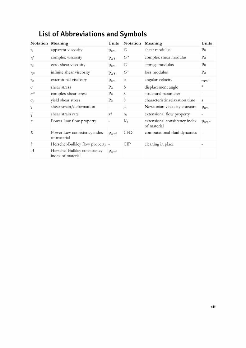
List of Abbreviations and Symbols Notation Meaning Units Notation Meaning Units

η apparent viscosity Paᐧs G shear modulus Pa

η* complex viscosity Paᐧs G* complex shear modulus Pa

η0 zero-shear viscosity Paᐧs G’ storage modulus Pa

η∞ infinite shear viscosity Paᐧs G’’ loss modulus Pa

ηε extensional viscosity Paᐧs ω angular velocity mᐧs-1

σ shear stress Pa δ displacement angle °

σ* complex shear stress Pa λ structural parameter -

σy yield shear stress Pa θ characteristic relaxation time s

γ shear strain/deformation - µ Newtonian viscosity constant Paᐧs γ ̇ shear strain rate s-1 nε extensional flow property -

n Power Law flow property - Kε extensional consistency index of material

Paᐧsnε

K Power Law consistency index of material

Paᐧsn CFD computational fluid dynamics -

b Herschel-Bulkley flow property - CIP cleaning in place -

A Herschel-Bulkley consistency index of material

Paᐧsb

1

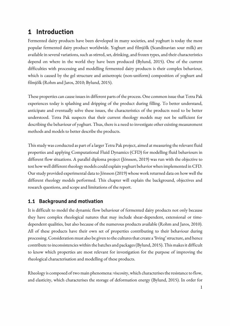
1 Introduction Fermented dairy products have been developed in many societies, and yoghurt is today the most

popular fermented dairy product worldwide. Yoghurt and filmjölk (Scandinavian sour milk) are

available in several variations, such as stirred, set, drinking, and frozen types, and their characteristics

depend on where in the world they have been produced (Bylund, 2015). One of the current

difficulties with processing and modelling fermented dairy products is their complex behaviour,

which is caused by the gel structure and anisotropic (non-uniform) composition of yoghurt and

filmjölk (Rohm and Jaros, 2010; Bylund, 2015).

These properties can cause issues in different parts of the process. One common issue that Tetra Pak

experiences today is splashing and dripping of the product during filling. To better understand,

anticipate and eventually solve these issues, the characteristics of the products need to be better

understood. Tetra Pak suspects that their current rheology models may not be sufficient for

describing the behaviour of yoghurt. Thus, there is a need to investigate other existing measurement

methods and models to better describe the products.

This study was conducted as part of a larger Tetra Pak project, aimed at measuring the relevant fluid

properties and applying Computational Fluid Dynamics (CFD) for modelling fluid behaviours in

different flow situations. A parallel diploma project (Jönsson, 2019) was run with the objective to

test how well different rheology models could explain yoghurt behavior when implemented in CFD.

Our study provided experimental data to Jönsson (2019) whose work returned data on how well the

different rheology models performed. This chapter will explain the background, objectives and

research questions, and scope and limitations of the report.

1.1 Background and motivation

It is difficult to model the dynamic flow behaviour of fermented dairy products not only because

they have complex rheological natures that may include shear-dependent, extensional or time-

dependent qualities, but also because of the numerous products available (Rohm and Jaros, 2010).

All of these products have their own set of properties contributing to their behaviour during

processing. Consideration must also be given to the cultures that create a ‘living’ structure, and hence contribute to inconsistencies within the batches and packages (Bylund, 2015). This makes it difficult

to know which properties are most relevant for investigation for the purpose of improving the

rheological characterisation and modelling of these products.

Rheology is composed of two main phenomena: viscosity, which characterises the resistance to flow,

and elasticity, which characterises the storage of deformation energy (Bylund, 2015). In order for

2

Tetra Pak to better meet the needs of its customers it requires a more robust set of test methods to

better define these elastic and viscous properties in addition to their current standardised test

methods. This would be useful for the construction and optimisation of filling machinery to

minimise issues like filamentation, dripping and splashing that can lead to the soiling of filling

equipment and causing a reduction in operating time and therefore plant efficiency and capacity.

Fermented dairy products have a tendency to stick to the interior surface of the packages. This makes

the customer unable to access the remaining yoghurt and leads to potential food waste. Improved

characterisation of the properties of yoghurt could potentially aid in minimising the interaction

between the yoghurt and the package surface and thus reduce food waste. The reduction of food

waste is a global issue which the UN encourages nations to address as one part of meeting its second

sustainable development goal of ‘zero hunger’, by 2030 (UN, 2017).

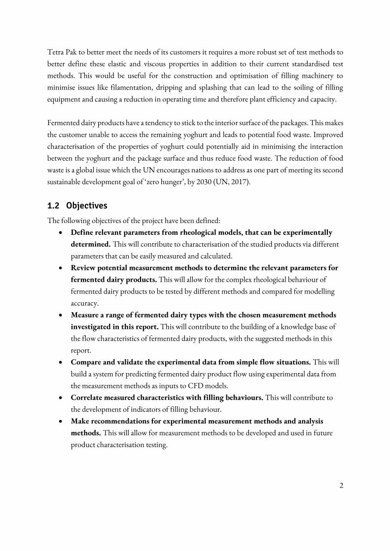
1.2 Objectives

The following objectives of the project have been defined:

• Define relevant parameters from rheological models, that can be experimentally

determined. This will contribute to characterisation of the studied products via different

parameters that can be easily measured and calculated.

• Review potential measurement methods to determine the relevant parameters for

fermented dairy products. This will allow for the complex rheological behaviour of

fermented dairy products to be tested by different methods and compared for modelling

accuracy.

• Measure a range of fermented dairy types with the chosen measurement methods

investigated in this report. This will contribute to the building of a knowledge base of

the flow characteristics of fermented dairy products, with the suggested methods in this

report.

• Compare and validate the experimental data from simple flow situations. This will

build a system for predicting fermented dairy product flow using experimental data from

the measurement methods as inputs to CFD models.

• Correlate measured characteristics with filling behaviours. This will contribute to

the development of indicators of filling behaviour.

• Make recommendations for experimental measurement methods and analysis

methods. This will allow for measurement methods to be developed and used in future

product characterisation testing.

3

1.3 Research questions

The project will aim to answer the following questions for a limited set of fermented dairy products:

1. Is it possible to measure the observable differences between the studied products with

existing measurement techniques and equipment?

2. In addition to dynamic viscosity, which parameters can be measured and shown to

contribute to the flow behaviour of yoghurt and thus yield a model anchored in reality?

3. Can issues in automatic filling, such as dripping and splashing, be anticipated using

measurable rheological properties?

1.4 Scope and limitations

The audience of this report is expected to include industrial researchers, Tetra Pak management,

academics and students with a similar academic background.

The following limitations on the scope of the project were identified:

• 20 weeks of full-time work

• Available measurement equipment is: rotational rheometers and hyperbolic contraction

flow rheometer (the limitations of the ranges and resolutions of the measurement

equipment can be found in Appendix 8.3)

• Maintaining exact consistency between samples will be difficult due to batch variations

• Tested parameters should be useful for fluid characterisation in CFD modelling

After considering the limitations described above, the scope of the project was set to include:

• Testing on a maximum of 3 different products

• To maximise the observable differences, the products will include:

○ Both high- and low-fat yoghurt types

○ A sample with added stabilisers

○ A sample with containing long polysaccharides

• To reduce unknown variables, the products will:

○ Be within a predefined range of shelf-life

○ Be plain- and stirred-type only

• Maximum two rigs for validation: ‘pulled plate rig’ and ‘filling rig’

The following were not investigated in this report, but may be relevant to future studies (including

but not limited to):

• The microstructure and particle size of the sample yoghurts

• Pre-shearing, to eliminate time dependent behaviour

4

• Temperature or pH dependence

• Composition: nutritional, gas (CO2), microbiological

The project described in this report involved three main phases: research, characterisation and

validation. Each phase had a discrete objective, as described in Figure 1.1, that contributed to the

completion of the overall project as well as the start of the subsequent phase. This project takes place

in the preliminary stages of the overarching Tetra Pak project described in § 1.

Figure 1.1 Simple flow chart of the required phases of the project described in this report.

1.5 Key deliverables

This project will aimed to satisfy both academic and industrial requirements. The key deliverables

for the University of Queensland and Lund University were:

• A project proposal describing the context, goals, scope and planned methodology of the

project, completed , due 07-03-2019

• An interim report detailing the progress of the project towards the planned outcome and

summarising any available results, due 02-05-2019

• A final report describing the work conducted during the course of the project and the

results, outcomes and recommendations of this work, due 07-06-2019

• A popular science summary of the methodology and results from the project, due 07-06-

2019

• A poster and presentation of the work undertaken during the project and outcomes, as

well as opposition to another student’s thesis presentation, due 04-06-2019

And for Tetra Pak they were:

• Descriptions of relevant measurement methods that can describe different types of

fermented milk products

• Assessments of constitutive viscosity models and parameters and how well they

describe the rheology of fermented milk products based on the results of the measurements

5

• Comparisons of the behaviour of different fermented milk products and correlation of

this behaviour to issues in filling

• A final report describing the work conducted during the course of the project and the

results, outcomes and recommendations of this work

2 Theoretical framework Fluids can be broadly categorised as either conventional, Newtonian fluids or complex, non-

Newtonian fluids. These two fluid categories are distinguished by how the viscosity changes with

shear rate and time. In this section, a review of literature regarding the application of various

rheological models to predict the flow of complex liquid foods will be presented. This is necessary

to accurately compare the rheological models used in this project, and the parameters they add as

they increase in complexity. Similarly, the methods for measuring the parameters were investigated

and will also be compared.

2.1 Rheological models

The most basic definition of viscosity was proposed by Isaac Newton as a constant which defined

the relationship between the rate of shear strain and the shear stresses experienced by the fluid under

strain, according to the equation (Morrison, 2001b): 𝜎 = 𝜇�̇� (1)

where σ is the shear stress in Pa, µ is the Newtonian viscosity constant in Paᐧs and γ̇ is the shear rate

in s-1. In this model, viscosity only varies with temperature. However, this model is often not

applicable to foods due to their gel structure and anisotropic compositions.

2.1.1 Shear-rate dependent models

Many fluids exhibit a decrease in viscosity as shear rate increases, which is referred to as shear-

thinning or pseudoplastic behaviour. After Newtonian behaviour, this is the most common

behaviour found in liquid food products (Morrison, 2001b; Mokhtari, 2011). In these cases, the

constants K [Paᐧsn] and n [-] describe the consistency and the flow respectively, according to the

equations: 𝜎 = 𝐾�̇�𝑛 (2) 𝜂 = 𝐾�̇�𝑛−1 (3)

where η is the non-Newtonian apparent viscosity in Paᐧs. This general expression, commonly

referred to as Power Law, for shear-dependent behaviour is adopted in many of the more complex

models but fails to account for the lack of flow exhibited by some fluids at very low shear stresses.

6

2.1.2 Yield stress models

An additional term is required to appropriately model the behaviour of some fluids which do not

flow at low shear stresses, such as fil and yoghurt. The simplest method is to introduce a yield stress,

σy [Pa], that describes the minimum stress required for the fluid to begin to flow (Stokes and Telford,

2004). The Bingham and Herschel-Bulkley models do this for Newtonian and Power Law fluids

respectively, resulting in the following equations (Mokhtari, 2011; Coussot, 2014): 𝜎 = 𝜎𝑦 + 𝜇�̇� (4) 𝜎 = 𝜎𝑦 + 𝐴�̇�𝑏 (5)

where the constants A [Paᐧsb] and b [-] also describe the consistency and the flow respectively. The

Herschel-Bulkley model was used by Fangary, Barigou and Seville (1999) in a similar experiment

focusing on predicting yoghurt viscosity immediately after filling, and it appeared to work well for

high shear rates.

However, the yield stress used is highly dependent on the time scale of observation (Cross, 1965).

Over longer time scales it is often found that the sample will begin to dissipate the applied stress and

very small flows can be observed. To account for these behaviours, a relationship between the

viscosity at very high or very low shear rates can be used (Chhabra, 2010). The Cross and Bird-

Carreau models both take this approach, with the following equations describing the viscosity in

each model, respectively: 𝜂 = 𝜂∞ + (𝜂0 − 𝜂∞)(1 + 𝐶�̇�)−𝑚 (6) 𝜂 = 𝜂∞ + (𝜂0 − 𝜂∞)(1 + 𝐶�̇�2)−𝑚/2 (7)

where η0 is the maximum viscosity as the shear rate approaches zero (zero-shear viscosity) in Paᐧs, η∞

is the limiting viscosity as the shear rate approaches infinity (viscosity at infinite shear rate) in Paᐧs,

and C and m are fitted constants. The applicability of the Cross model in particular has been

explored by Javanmard et al. (2018) on milk-based gels and by Butler and McNulty (1995) on

buttermilk.

2.1.3 Time-dependent models

In addition to being dependent on shear rate, the viscosity of complex fluids is also often dependent

on time. This dependence is described by several thixotropic-viscoplastic (TVP) models, including

the Kelvin, Maxwell, Coussot, Gumulya and Tiu-Boger models, which were the most commonly

used when modelling food (Moller et al., 2009; Gumulya, Horsley and Pareek, 2014). In addition to

being dependent on the time scale of exposure to stress or strain, some fluids exhibit shear history

behaviour where a fluid exhibits a different viscosity at a given shear rate if it has recently been

subjected to a much higher shear rate. If the viscosity of the fluid is decreased by these memory

7

effects, then it can be referred to as thixotropic, with the opposite being rheopectic (Bergenståhl et

al., 2007).

The Coussot, Gumulya and Tiu-Boger methods all introduce a time-dependent structural

parameter to describe this shear history-dependent behaviour, although the implementation varies

(Rohm and Jaros, 2010; Butler and McNulty, 1995). This structural parameter, λ [-], describes how

much of the initial structure of the fluid remains intact at a given point in time, and has been defined

with relation to an equilibrium value of the structural parameter, λe [-] (Javanmard et al., 2018;

Mokhtari, 2011), and as a function of the characteristic relaxation time of the fluid, θ [s], and shear

rate (Gumulya, Horsley and Pareek, 2014). In the second case, which was explored in this work, the

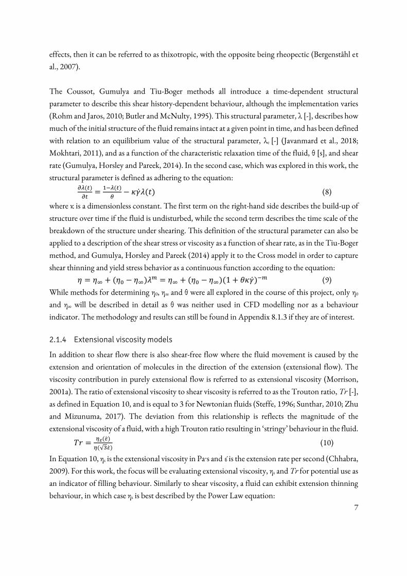
structural parameter is defined as adhering to the equation:

𝜕𝜆(𝑡)𝜕𝑡 = 1−𝜆(𝑡)𝜃 − 𝜅�̇�𝜆(𝑡) (8)

where κ is a dimensionless constant. The first term on the right-hand side describes the build-up of

structure over time if the fluid is undisturbed, while the second term describes the time scale of the

breakdown of the structure under shearing. This definition of the structural parameter can also be

applied to a description of the shear stress or viscosity as a function of shear rate, as in the Tiu-Boger

method, and Gumulya, Horsley and Pareek (2014) apply it to the Cross model in order to capture

shear thinning and yield stress behavior as a continuous function according to the equation:

𝜂 = 𝜂∞ + (𝜂0 − 𝜂∞)𝜆𝑚 = 𝜂∞ + (𝜂0 − 𝜂∞)(1 + 𝜃𝜅�̇�)−𝑚 (9)

While methods for determining η0, η∞ and θ were all explored in the course of this project, only η0

and η∞ will be described in detail as θ was neither used in CFD modelling nor as a behaviour

indicator. The methodology and results can still be found in Appendix 8.1.3 if they are of interest.

2.1.4 Extensional viscosity models

In addition to shear flow there is also shear-free flow where the fluid movement is caused by the

extension and orientation of molecules in the direction of the extension (extensional flow). The

viscosity contribution in purely extensional flow is referred to as extensional viscosity (Morrison,

2001a). The ratio of extensional viscosity to shear viscosity is referred to as the Trouton ratio, Tr [-],

as defined in Equation 10, and is equal to 3 for Newtonian fluids (Steffe, 1996; Sunthar, 2010; Zhu

and Mizunuma, 2017). The deviation from this relationship is reflects the magnitude of the

extensional viscosity of a fluid, with a high Trouton ratio resulting in ‘stringy’ behaviour in the fluid. 𝑇𝑟 = 𝜂𝜀(�̇�)𝜂(√3�̇�) (10)

In Equation 10, ηε is the extensional viscosity in Paᐧs and ε̇ is the extension rate per second (Chhabra,

2009). For this work, the focus will be evaluating extensional viscosity, ηε and Tr for potential use as

an indicator of filling behaviour. Similarly to shear viscosity, a fluid can exhibit extension thinning

behaviour, in which case ηε is best described by the Power Law equation:

8

𝜂𝜀 = 𝐾𝜀𝜀̇𝑛𝜀−1 (11)

2.2 Shear rheological parameter determination

A rotational rheometer using cup-and-bob geometry was used for most of the characterisation and

the most common existing methods were researched and have been described in the sections below.

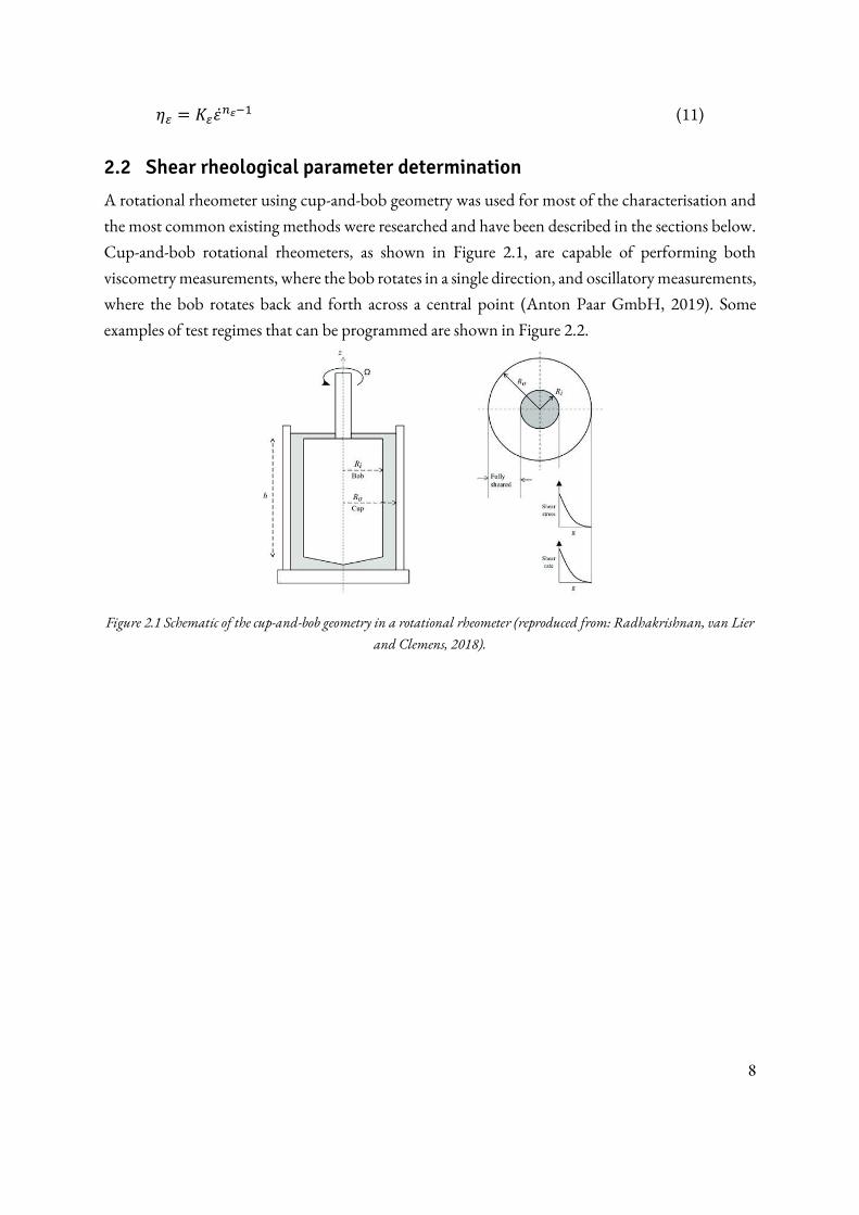
Cup-and-bob rotational rheometers, as shown in Figure 2.1, are capable of performing both

viscometry measurements, where the bob rotates in a single direction, and oscillatory measurements,

where the bob rotates back and forth across a central point (Anton Paar GmbH, 2019). Some

examples of test regimes that can be programmed are shown in Figure 2.2.

Figure 2.1 Schematic of the cup-and-bob geometry in a rotational rheometer (reproduced from: Radhakrishnan, van Lier

and Clemens, 2018).

9

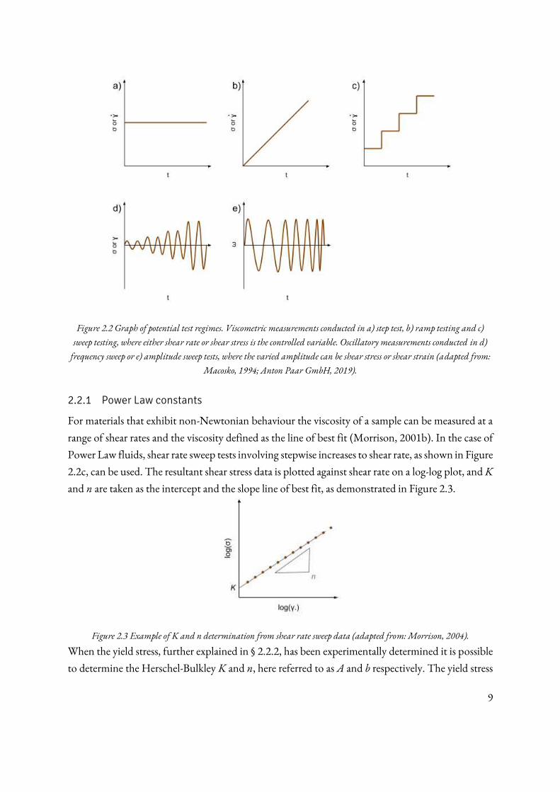
Figure 2.2 Graph of potential test regimes. Viscometric measurements conducted in a) step test, b) ramp testing and c)

sweep testing, where either shear rate or shear stress is the controlled variable. Oscillatory measurements conducted in d)

frequency sweep or e) amplitude sweep tests, where the varied amplitude can be shear stress or shear strain (adapted from:

Macosko, 1994; Anton Paar GmbH, 2019).

2.2.1 Power Law constants

For materials that exhibit non-Newtonian behaviour the viscosity of a sample can be measured at a

range of shear rates and the viscosity defined as the line of best fit (Morrison, 2001b). In the case of

Power Law fluids, shear rate sweep tests involving stepwise increases to shear rate, as shown in Figure

2.2c, can be used. The resultant shear stress data is plotted against shear rate on a log-log plot, and K

and n are taken as the intercept and the slope line of best fit, as demonstrated in Figure 2.3.

Figure 2.3 Example of K and n determination from shear rate sweep data (adapted from: Morrison, 2004).

When the yield stress, further explained in § 2.2.2, has been experimentally determined it is possible

to determine the Herschel-Bulkley K and n, here referred to as A and b respectively. The yield stress

10

is subtracted from the measured stress and curve fitting is then performed as described above to

determine A and b.

2.2.2 Yield stress

Several measurement and analysis methods exist for determining the shear yield stress, σy, of a sample

using a rotational rheometer, although determination of a ‘true’ yield stress can be difficult (Moller

et al., 2009). A linear stress ramp starting from low stress is one measurement method, with several

yield stress analysis options available. The simplest and easiest to perform is to take the value of the

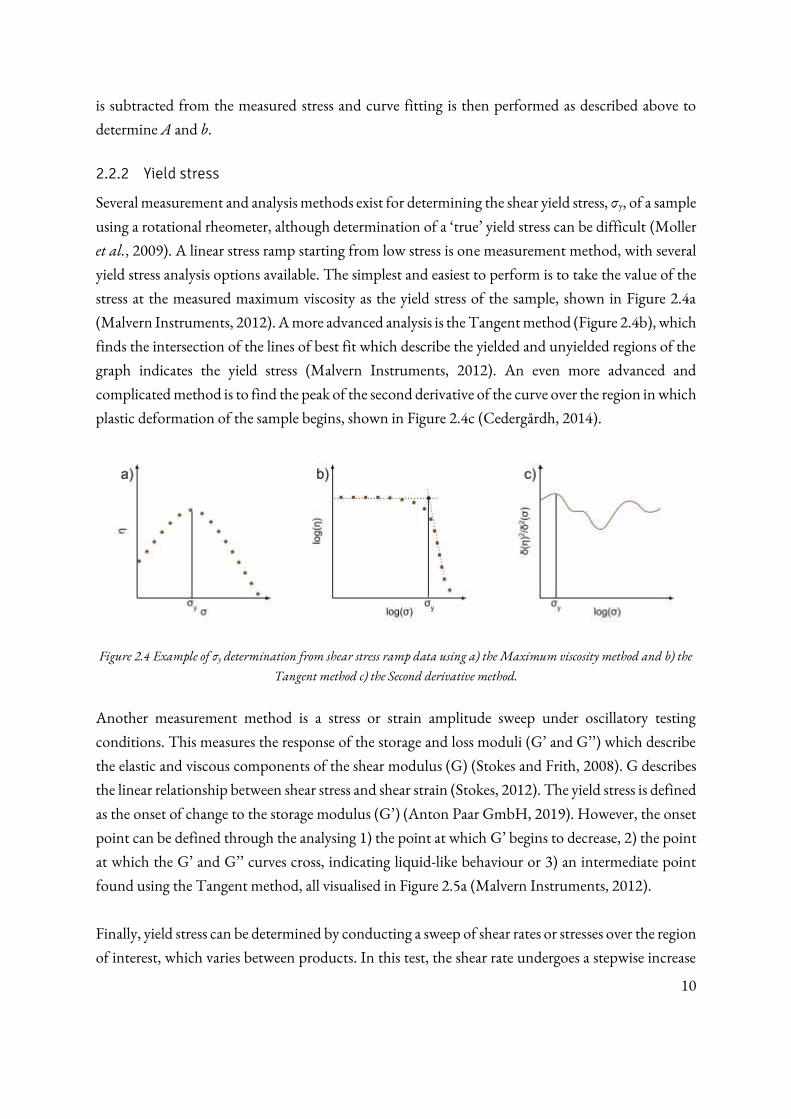
stress at the measured maximum viscosity as the yield stress of the sample, shown in Figure 2.4a

(Malvern Instruments, 2012). A more advanced analysis is the Tangent method (Figure 2.4b), which

finds the intersection of the lines of best fit which describe the yielded and unyielded regions of the

graph indicates the yield stress (Malvern Instruments, 2012). An even more advanced and

complicated method is to find the peak of the second derivative of the curve over the region in which

plastic deformation of the sample begins, shown in Figure 2.4c (Cedergårdh, 2014).

Figure 2.4 Example of σy determination from shear stress ramp data using a) the Maximum viscosity method and b) the

Tangent method c) the Second derivative method.

Another measurement method is a stress or strain amplitude sweep under oscillatory testing

conditions. This measures the response of the storage and loss moduli (G’ and G’’) which describe the elastic and viscous components of the shear modulus (G) (Stokes and Frith, 2008). G describes

the linear relationship between shear stress and shear strain (Stokes, 2012). The yield stress is defined

as the onset of change to the storage modulus (G’) (Anton Paar GmbH, 2019). However, the onset

point can be defined through the analysing 1) the point at which G’ begins to decrease, 2) the point

at which the G’ and G’’ curves cross, indicating liquid-like behaviour or 3) an intermediate point

found using the Tangent method, all visualised in Figure 2.5a (Malvern Instruments, 2012).

Finally, yield stress can be determined by conducting a sweep of shear rates or stresses over the region

of interest, which varies between products. In this test, the shear rate undergoes a stepwise increase

11

and the sample is then given time to equilibrate before a measurement is taken. Previous study

conducted on fermented dairy products have shown that true equilibrium will not be achieved as

the samples are expected to continue to exhibit shear thinning behaviour for more than 1 hour

(Butler and McNulty, 1995). The Tangent analysis method can again be applied here, or the stress

at the minimum value of the first derivative of the ratio of logarithms of shear stress to shear strain

can also be taken (Figure 2.5b) (Mendes and Dutra, 2004; Bayod et al., 2007).

Figure 2.5 Example of σy determination from a) stress amplitude sweep data using three different analysis methods

(adapted from: Malvern Instruments, 2012) and b) shear rate or shear stress sweep tests using the Mendes and Dutra

(2004) or Bayod (2007) methods.

2.2.3 Zero-shear viscosity

The zero-shear viscosity, η0, refers to the apparent viscosity plateau of the sample within the linear

viscoelastic region (LVER) which occurs at very low shear rates, well below the yield stress. This can

be measured in both oscillatory tests and transient tests where the strain amplitude or shear stress are

kept within the LVER. If the apparent viscosity measured in these tests is plotted against strain or

shear stress, η0 can be seen as the linear plateau as depicted in Figure 2.6a (Anton Paar GmbH, 2019).

Another method for determining the zero-shear viscosity is to conduct a sweep of shear rates from

extremely low shear rates. At very low shear rates, the viscosity as a function of shear stress or shear

rate will be constant and equal to the zero-shear viscosity (Mendes and Dutra, 2004). Therefore, it

can be determined by defining a tangent along the plateau as described in Figure 2.6b. The zero-shear

viscosity should be independent of both time and shear rate, if the fluid conforms to time-

independent models such as the Cross model, although it will be dependent on temperature.

A final method for zero-shear viscosity determination is creep testing, where the shear strain is

measured over time as it responds to the application of a constant shear stress. The applied stress

should be within the LVER, and the zero-shear viscosity is found by taking the inverse of the slope

12

when the sample is exhibiting viscous flow behaviour (Morea, Agnusdei and Zerbino, 2010), as

shown in Figure 2.6c.

Figure 2.6 Example of η0 determination using a) and b) plateau analysis on shear stress or strain amplitude or shear rate

controlled test data (adapted from: Anton Paar GmbH, 2019; Mendes and Dutra, 2004) and c) slope analysis on creep

test data (adapted from: Morea, Agnusdei and Zerbino, 2010).

2.2.4 Viscosity at infinite shear rate

Just as the zero-shear viscosity describes the fluid behaviour under very low shear rates, the viscosity

at infinite shear rate describes the second viscosity plateau that occurs as the fluid is subjected to very

high shear rates or frequencies (Cross, 1965). A method developed by Cross (1965) was intended to

be applied to frequency sweeps in order to determine these parameters. The Cross method plots

apparent viscosity as a function of shear rate or frequency and includes a region of constant shear

thinning (adhering to the Power Law) between the viscosity plateaus. However, the two plateau

regions were not located in the range of frequencies tested in this study.

Due to difficulties in applying the Cross method, this work attempted to define the viscosity at

infinite shear rate as the viscosity when shear rate and time approach infinity using a constant shear

rate (CSR) test, as depicted in Figure 2.7. The reasoning behind using these tests was that η∞

represents the lowest possible viscosity for the fluid and could therefore be approximated by

maximising the shear-thinning and minimising time-dependent effects experienced by the fluid. The

use of the highest laminar shear rates allowed by the equipment for long times was used to predict

the lowest possible viscosity that the product may be expected to reach. The method developed in

this study for estimating η∞ is therefore constrained by the development of turbulent flow in the

geometry used.

The viscosity at infinite shear rate is often lower than the zero-shear viscosity by several orders of

magnitude in shear thinning fluids and is therefore often neglected in models by assuming a viscosity

13

of 0 Paᐧs (Gumulya, Horsley and Pareek, 2014). Where a limiting viscosity is required for modelling,

it may be sufficient to assume the viscosity of water or milk.

Figure 2.7 Example of η∞ determination using plateau analysis on CSR data conducted at the highest possible shear rate.

2.2.5 Relaxation time

The relaxation time (θ) describes how quickly the sample reacts to the application of external force

and can be found using oscillatory tests within the LVER. When performing frequency sweep tests

in small amplitude oscillation (SAOS) testing, the relaxation time is the inverse of the frequency at

which the storage modulus, G’, and the loss modulus, G’’, intersect as shown in Figure 2.8.

Relaxation time can also be calculated as the time required for the shear stress to reach ~63% of its

maximum value in a relaxation test. When conducting these experiments on gels, G’ and G’’ should produce curves that run parallel inside the LVER (Franck, n.d.; Bayod, 2008). The relaxation time

may also be a model-dependent property, being determined by fitting a model curve to the measured

data points for a shear rate sweep test or similar.

Figure 2.8 Example of θ determination using frequency sweep data.

14

2.2.6 Thixotropy

In addition to determining θ as a modelling parameter, the time-dependent nature of the products

can also be confirmed through hysteresis loops and varied shear rate tests (Tehrani, 2008; Landman,

2019). Both tests function by exposing the product to high shear rates and then returning to lower

shear rates and observing the difference in viscosity at the same shear rate. The hysteresis loop test

performs a shear rate sweep (as in Figure 2.2c) progressing from low shear rates to high, referred to

as the ‘upward’ sweep, then returning again to low shear rates, the ‘downward’ sweep. The data

points are taken when an approximate equilibrium in the viscosity has been reached, which neglects

any initial changes in the viscosity as the shear rate is stepped up or down.

The varied shear rate tests focus on the stress response of the product to these steps in shear rate.

Shear rate is alternated between varying high and low values and the transient responses of the

product are recorded. Both methods are useful for assessing whether a product displays time-

dependency but focus on different aspects of this behaviour.

2.3 Extensional rheological parameter determination

Measurement methods for determining the extensional viscosity in fluids are relatively new, but

capillary breakup and contraction flow are two existing methods. Visual representations of two

equipment types are shown in Figure 2.9.

Figure 2.9 Schematics of a HCF extensional rheometer (left) (Reproduced from: Nyström et al., 2017) and capillary

breakup extensional rheometer (Reproduced from: Thermo Scientific, 2015).

2.3.1 Extensional viscosity

Testing under low-shear conditions in a hyperbolic contraction flow rheometer (HCF) can yield a

viscosity profile that can be separated into shear and extensional viscosity by methods such as the

Cogswell, Bagley or Binding analyses (Stading and Bohlin, n.d.; Nyström et al., 2017). For example,

using the Cogswell analysis the extensional viscosity, ηε [Paᐧs], and extension rate, ε̇ [s-1], can be

15

described as a function of pressure drop at the entrance, ΔPe [Pa] of an axisymmetric contraction

according to the equations (Larson, 1994): 𝜂𝜀 = 9(𝑛 + 1)2(𝛥𝑃𝑒)2(32𝜂�̇�)−2 (13) 𝜀 = (4𝜂�̇�)2(3(𝑛 + 1)𝛥𝑃𝑒)−1 (14)

where n is a constant. In the HCF rheometer the hyperbolic geometry of the nozzle is designed to

minimise the contribution of shear effects, with a constant rate of displacement being applied to the

sample being moved through the nozzle, or contraction (Nyström et al., 2017). The normal forces

as the fluid moves through the contraction are measured by a load cell mounted above the nozzle.

A similar method can be used in capillary breakup rheometry, where the normal forces and capillary

diameter are measured (Thermo Scientific, 2015). The advantage of the HCF is that the sample is

not exposed to the environment, however this comes at the cost of the measured viscosity being

highly dependent on the outlet radius of the die.

16

3 Methodology This section will explain the experimental methodologies used for each instrument used during this

study. If not stated otherwise, all measurements were performed at 20°C.

In total, 13 parameters were to be determined experimentally, with the aim of being used for CFD

modelling of the fluid models described in § 2 and qualitative correlation to filling behaviour in

subsequent validation tests. The parameters are summarised in Table 3.1.

Table 3.1 Measured parameters.

Parameters Required for

K, n, η(100 s-1, 20°C) Power Law

A, b, η(100 s-1, 20°C) Herschel-Bulkley

σy

η0 TVP Boundary conditions for Herschel-Bulkley and Power Law η∞

Kε, nε, ηε(100 s-1, 20°C), Tr Behaviour indicators (for filling behaviour)

3.1 Sample preparation and handling

The samples used were packaged fermented dairy products selected to meet the criteria given in §

1.4. All products were bought from local supermarkets and stored in a refrigerator at ~6°C when not

used. The following products were selected and used for testing (Figure 3.1):

• 1 kg Skånemejerier Vaniljyoghurt (2.5 % fat) Ingredients: Pasteurized milk, sugar 6.5%, modified corn starch, stabilizer (pectin), aroma, acid

(citric acid), natural vanilla aroma, yoghurt culture

• 1 kg Skånemejerier Naturell Lättyoghurt (0.5 % fat) Ingredients: Pasteurized milk, milk protein, yoghurt culture, vitamin D

• 1 kg Arla Långfil (3.0 % fat) Ingredients: Pasteurized milk, fil culture, vitamin D

The above products will be referred to as Vanilj, Naturell and Långfil, respectively. Note that Vanilj

contains added starch and stabilisers, Naturell contains added milk protein and Långfil contains a

different culture than the yoghurt samples, which results in exopolysaccharides (high molecular

weight polymers) after fermentation (Fondén, Leporanta and Svensson, 2006).

17

Figure 3.1 Images of the three products studied in this thesis. From left to right, Vanilj, Naturell and Långfil

The samples were compared by age using a CSR test (Appendix 8.1.5). From that it was decided that

Naturell and Långfil should be used within 5 days after opening. Vanilj did not display any

significant difference during these comparisons and could therefore be used until its best before date.

A sample handling technique was established to improve the reproducibility of the results. Several

variables were considered, including:

• Sample homogenisation

• Stabilisation time

• Pre-shearing

• Resting time

• Sample volume

• Instrument geometry

• Gap height and lowering rate of geometry

Sample homogenisation was achieved according to Table 3.2. ‘Inversion’ refers to tilting the package 180° vertically downwards and then back up 180°, and ‘stir’ refers to moving a long spoon through

the sample for one full clockwise rotation. Långfil proved to be more difficult to homogenise than

Vanilj and Naturell and was therefore carefully transferred to a resealable transparent glass jar after

the 40 inversions. This facilitated the homogenisation of Långfil and made it obvious when whey

separation started to occur.

Stabilisation time for sweep tests was determined according to a method developed internally at

Tetra Pak, using data collected from CSR tests. This method found the time required for the

difference in viscosity over 10 s time period to drop below 5 % (see Figure 3.2). The time required

18

was defined as the stabilisation time. When the difference in viscosity of the products dropped below

5 % during a 10 s interval, it was assumed that the difference was low enough to be considered an

equilibrium state. By applying the stabilisation time to the performed measurements, it was possible

to collect data from an equilibrium state. The stabilisation times for each product can be found in

Table 3.2.

Figure 3.2 Graph of the CSR test for Vanilj (replicate 1). The arrows point to the 10 second interval at the time required

for the difference in viscosity to drop below 5 % (40 seconds).

No additional pre-shearing was performed on the samples at any time as the scope included the

measurement and modelling of time-dependent effects, which would have been diminished by pre-

shearing.

The sample volume was controlled in the cup-and-bob geometry by using a 15 mL measuring cup

to load the samples. A resting time of 60 s was used for all products during characterisation

measurements (Table 3.2). Serrated bob-and-cup geometry was used after a performed comparison

with smooth bob-and-cup geometry. The comparison implied no significant difference between the

used geometries, but the serrated geometry was used when possible (excluding TA ARES rotational

rheometer and HCF rheometer) to minimise potential wall-slip effects. There was no calibration

performed prior to any measurements with the serrated bob and cup geometry. Additionally, the

default settings of the gap height and lowering rate of geometry was used for all the performed

measurements.

Table 3.2 Established sample homogenisation methods, stabilisation times and resting times.

Conditions Vanilj Naturell Långfil

Inversions after purchase 10 10 40

Inversions/stirs prior to loading 2 2 2

10 s

19

Stabilisation time [s] 40 60 90

Resting time [s] 60 60 60

3.2 Rotational rheometer

The following sections detail the materials and test parameters for characterisation measurements

conducted using the Kinexus rotational rheometer (Figure 3.3). The operating conditions specified

in § 3.2.2-3.2.7 refer to the inputs that are required by the rSpace software at the beginning of the

relevant test sequence. A detailed methodology for the use of the Kinexus rheometer and

descriptions of the available test sequences and operating conditions can be found in Appendices

8.1.1 and 8.1.2.

3.2.1 Materials

• Temperature controlled Malvern Kinexus rheometer (Malvern Instruments limited

Worcestershire UK)

• rSpace for Kinexus software

• Serrated bob geometry, 25 mm diameter, C25G A0009 SS

• Serrated cup geometry, 27.5 mm diameter, PC25G A0008 AL

20

Figure 3.3 From left to right: images of the Malvern Kinexus rotational rheometer, serrated 25 mm bob and serrated

3.2.2 Power Law curve fitting

The Power Law variables K and n were determined as explained in § 2.2.1. The operating conditions

have been compiled in Table 3.3 along with the required data, analysis method and measurement

method.

Table 3.3 Determination methods for Power Law constants.

Required Data Parameters Analysis Method Model Measurement method

Operating Conditions

σ(γ ̇) K, n Curve fitting Power Law Shear rate sweep

Shear rate range: 0.7-700 s-1

Samples per decade: 7

3.2.3 Yield stress

The yield stress was determined using six different methods, as explained in § 2.2.2. Each analysis

method requires a specific measurement method. The operating conditions for each measurement

method have been compiled in Table 3.4 along with the required data and analysis method. While

all methods were tested, the Tangent and Bayod methods, using shear stress-controlled data, were

chosen for further analysis and use in modelling. This was required since time did not allow for all

the results to be included in the CFD modelling.

The Mendes & Dutra and Tangent using strain-controlled data methods were excluded from

consideration as stress-controlled data is preferable for the determination of yield stress as there is no

possibility for overlap in the measured stress. Similarly, the Maximum viscosity method was the

simplest method, but the range of stresses which produced viscosities close to the maximum was too

broad to definitively choose a single point. The Second derivative method was very promising, but

the analysis method was unable to cope with the oscillations present in the raw data and was

unfortunately unable to be used consistently.

Table 3.4 Determination methods for yield stress.

Required Data Analysis Method Measurement Method


η(σ) Maximum viscosity Linear stress ramp

Ramp time: 20 min Stress range: 1-10 Pa Tangent

21

Second derivative Sampling interval: 1 s

σ(γ ̇) Mendes & Dutra (first derivative) Shear rate sweep

Shear rate range: 1×10-4-1×103 s-1


γ ̇ (σ) Bayod (first derivative) Shear stress sweep

Shear stress range: 1-10 Pa Samples per decade: 20

G’(γ) Tangent Shear strain amplitude sweep

Shear strain range: 0.001-1 Samples per decade: 10

3.2.4 Herschel-Bulkley curve fitting

The Herschel-Bulkley variables A and b were determined the same way as the Power Law variables

K and n (as explained in § 2.2.1), with the exception of an included yield stress (see Equation 5) and

curve fitting to a shear rate range of 7-700 s-1, due to negative shear stress values occurring below this

range. The operating conditions have been compiled in Table 3.5 along with the required data and

analysis method.

Table 3.5 Determination methods for Herschel-Bulkley constants.

Required Data Parameters Analysis Method Measurement Method


σ(γ ̇)

A, b Curve fitting

Shear rate sweep

Shear rate range: 7-700 s-1


Yield stress determination

As explained in § 3.2.3 σy


The zero-shear viscosity was determined by three different methods, as explained in § 2.2.3. Each

analysis method requires a specific measurement method. The operating conditions for each

measurement method have been compiled in Table 3.6 along with the required data and analysis

method.

Table 3.6 Determination methods for zero shear viscosity.



η(σ) Plateau (log) Shear stress sweep

Shear stress range: 1-10 Pa Samples per decade: 20

22

η(γ ̇) Shear rate sweep

Shear rate range: 0.0001-1000 s-1


ɣ(t) Inverse of slope of creep curve

Creep and relaxation test

Creep time: 5 min Relaxation time: 0 min Shear stress: 1 Pa Samples per decade: 20 Number of times to run: 1


The viscosity at infinite shear rate was determined as explained in § 2.2.4. The highest laminar shear

rate for Vanilj and Naturell was 1500 s-1 while for Långfil it was 2500 s-1. Since the viscosity at infinite

shear rate is only used as a boundary condition for high-shear flows, the viscosity at infinite shear

rate could potentially be set to 0 Paᐧs if these conditions are not relevant to the model. However,

since a viscosity of 0 Paᐧs is highly unrealistic the boundary condition could instead be assumed to

be the viscosity of either water or milk. The operating conditions have been compiled in Table 3.7

along with the required data and analysis method.

Table 3.7 Analysis methods for determination of zero shear viscosity, required data and measurement method for each

analysis method.



η(γ ̇)

Find η when t, γ ̇ → ∞

Shear rate ramp

Shear rate range, Vanilj & Naturell: 300-3000 s-1

Shear rate range, Långfil: 700-7000 s-1 Ramp time: 5 min Samples per decade: 20

η(t)

Constant shear rate

Shear rate, Vanilj & Naturell: 1500 s-1

Shear rate, Långfil: 2500 s-1 Time: 900 s Sampling interval: 1 s

- Assume η∞ = 0, or η∞ = water/milk -

3.2.7 Thixotropy

The thixotropic nature of yoghurt was confirmed by performing hysteresis loop testing and varied

shear rate testing. The varied shear rate testing was conducted using a method adapted from

Landman (2019) to both visualise the break-down and build-up of the sample structure and to

provide data for model fitting and validation. The operating conditions have been compiled in Table

23

3.8 along with the required data and analysis method. Unsuccessful attempts were also made to

quantify the characteristic relaxation time (θ) which may be used to predict thixotropic effects,

further described in Appendix 8.1.3.

24

Table 3.8 Analysis methods, required data and measurement method for the determination of thixotropic behaviour.

Required Data Analysis Method Measurement method


σ(γ ̇) Hysteresis loop plots Shear rate sweep, up and down

Shear rate range: 0.7-700 s-1 then 700-0.7 s-1


σ(γ ̇) Varied shear rate

Varied shear rate testing Shear rate steps: 1 s-1

for 120 s 300 s-1

for 30 s 0.01 s-1

for 120 s 70 s-1

for 300 s 0.1 s-1

for 120 s 100 s-1

for 30 s 0.001 s-1

for 120 s 500 s-1

for 30 s 0.01 s-1

for 120 s 300 s-1

for 30 s

3.3 Extensional rheometer

The following sections detail the materials and test parameters for characterisation measurements

conducted using the HCF rheometer (Figure 3.4). A detailed methodology for the use of the HCF

rheometer can be found in Appendix 8.1.4.

3.3.1 Materials

• Instron tensile tester (Instron, Norwood, MA, USA)

• Hyperbolic contraction flow geometry (fabricated in-house)

• Bluehill 2 version 2.6 software with extensional viscosity add-on (Instron, Norwood, MA,

USA)

• TA ARES strain controlled rotational rheometer (TA Instruments, New Castle, DE, USA)

• TRIOS Software version 3.3.0.4055 (TA Instruments, New Castle, DE, USA)

• Smooth parallel plate geometry, 402282.001 (TA Instruments, New Castle, DE, USA)

• Two temperature-controlled water baths (Julabo Labortechnik GmbH)

• Hyperbolic contraction nozzle with exit radius 0.75 mm

• Hyperbolic contraction nozzle with exit radius 2.15 mm

25

Figure 3.4 Images showing (clockwise from left) Instron extensional rheometer where a) is the load cell, b) is the load cell

adaptor, c) is the sample cell and cooling jacket and d) is the piston, hyperbolic contraction nozzle (0.75 mm die) outlet

and inlet.

3.3.2 Extensional viscosity

The Power Law variables K and n was determined as explained in § 2.2.1. The K and n values was

then used in the software for the calculation of the corrected extensional viscosity, as explained in §

2.3.1. The operating conditions have been compiled in Table 3.9 along with the required data,

analysis method and measurement method.

Table 3.9 Required data, analysis method, measurement method and operating conditions for Kε and nε determination.

Required data Parameters Analysis method Measurement method

Operating conditions

η(γ ̇) K, n Power Law curve fitting

ARES rheometer: Shear rate sweep

Shear rate range: 1-100 s-1


Gap height: 1 mm

Stabilisation time: <15 s (all samples)

K, n

Kε, nε ηε-correction,

Power Law curve fitting

HCF: Extensional sweep up and down

Piston displacement rate: 0.6-6.0 mm/s Equivalent extension rate: 1-100 s-1

Samples per decade: 5 ηε(ε̇)

26

3.4 Pulled plate rig and laser profiler

The following sections detail the materials and operating conditions for the measurement of the

product flow profile on a vertical stainless-steel plate (Figure 3.5). A detailed methodology can be

found in Appendix 8.2.1.

3.4.1 Materials

• Instron tensile tester (Instron, England)

• Bluehill software for tensile tester

• 1 liter plastic box (as sample vessel)

• Stainless steel plate, 10×15×0.2 cm3 (Fabricated in-house, Tetra Pak AB, Sweden)

• Camera tripod

• Micro-epsilon scanCONTROL 2950-100 laser profiler (Micro-Epsilon)

• Micro-epsilon software for laser profiler (Micro-Epsilon)

Figure 3.5 Image of the set-up of the pulled plate rig showing a) the load cell, b) the pneumatic grip, c) the stainless-steel

plate, d) the product container, f) the laser profiler and g) the tripod laser profiler stand.

3.4.2 Operating conditions

Each test consisted of 5 cycles before cleaning the plate, meaning that the first cycle always used a

clean plate and the subsequent cycles did not. Triplicate tests were performed on two different

packages for each product, meaning six replicates for each product. The following sequence for a

single cycle was used in this study:

28

• Plate lowered 70 mm at 15 mm/s

• Plate incubated for 60 s

• Plate pulled up 70 mm at 15 mm/s

• Plate left hanging for minimum 60 s

3.4.3 Data treatment

The raw data from the tensile tester and laser scanner were exported separately. The data from the

laser scanner could be analysed without reference to the tensile tester by plotting the first point on

the plate over the full range of time. The point at which the plate came to a rest while hanging could

then be identified from the curves, such as the example shown in Figure 3.6. The raw data for the

surface profile contained significant noise as the sampling frequency was 6 s-1. The noise was reduced

by creating a 10-point moving average of the surface profile. The top 50 mm of the plate was not

submerged in the sample so that it could be used to define a reference point for the calculation of

the profile thickness. The constants from a linear regression across this region were used to calculate

the average distance to the plate at each point, from which the measured distance was subtracted to

find the profile thickness.

Figure 3.6 Graph of the first point of laser profile over time for determining start of hang time (indicated by the arrow).

3.5 Stand-alone filling rig

The following sections detail the materials and test parameters for the fill rig testing (Figure 3.7). A

detailed methodology can be found in Appendix 8.2.2.

1 cycle 0 seconds hang time

29

3.5.1 Materials

• Stand-alone filling rig: Tetra Top One Shot (Tetra Pak AB, Sweden)

• Digital camera on iPhone (Tetra Pak AB, Sweden)

• Image analysis software (Windows Media Player, Microsoft Corporation)

Figure 3.7 Image of the stand-alone fill rig setup showing a) the fill nozzle, b) the transparent ‘package’, c) the

transparent splash plate, d) the bottom drain for the transparent package.

3.5.2 Operating conditions

The operating conditions used during the fill rig tests are displayed in Table 3.10 below.

Table 3.10 Descriptions of the operating conditions used during fill rig testing.

Setting Volume Cam curve

Standard (STD) 200 mL ID 1

Modified (MOD) 250 mL ID 4

During one filling shot, the bottom drain was closed and the package was raised towards the fill

nozzle (from its default level) and filling began. The STD setting then held the package at this height

during filling and rapidly lowered the package to the default level after filling was complete, while

the MOD setting slowly lowered the package during filling. One filling shot took 1.6 s. After this,

30

the bottom drain was opened and the product was empties from the package, which took a further

1.6 s. For Långfil, the emptying time had to be prolonged manually to prevent product buildup in

the package.

3.5.3 Quantification and statistical analyses

Filling issues were quantified both by counting visible residues during testing and by analysing the

high-speed video after testing was complete. This video analysis was used to first define filling events

and issues and then to quantify them by counting the number of occurrences per 10-fill cycles.

The rheological parameters measured in § 3.2 and 3.3 were analysed with the results from the fill rig

tests in order to identify potential indicators for problematic filling behaviours. One multivariate

statistical analysis was performed in Excel with the available Data Analysis Tools (‘correlation’), based on Pearson correlation coefficients. The results from that analysis can be found in Appendix

8.2.3 (Table 8.7). Another multivariate statistical analysis, the Partial Least Square or Projection to

Latent Structures (PLS), was performed in MATLAB. In the PLS analysis the studied products are

referred to as ‘observations’, the determined rheological parameters are referred to as ‘variables’ and the observed issues are referred to as ‘responses’. The parameters were chosen to be the variables and

the issues were chosen to be the responses, as it was expected that the issues were dependent on some

of these parameters. The correlation was done with the help of a biplot (W*Q plot), where the

variables and responses are plotted simultaneously as explained by Håkansson (2018).

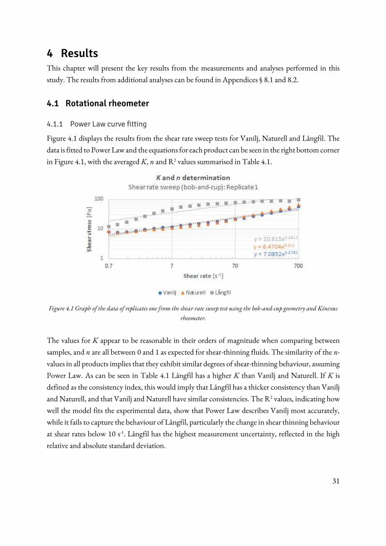
31

4 Results This chapter will present the key results from the measurements and analyses performed in this

study. The results from additional analyses can be found in Appendices § 8.1 and 8.2.

4.1 Rotational rheometer

4.1.1 Power Law curve fitting

Figure 4.1 displays the results from the shear rate sweep tests for Vanilj, Naturell and Långfil. The

data is fitted to Power Law and the equations for each product can be seen in the right bottom corner

in Figure 4.1, with the averaged K, n and R2 values summarised in Table 4.1.

Figure 4.1 Graph of the data of replicates one from the shear rate sweep test using the bob-and-cup geometry and Kinexus

rheometer.

The values for K appear to be reasonable in their orders of magnitude when comparing between

samples, and n are all between 0 and 1 as expected for shear-thinning fluids. The similarity of the n-

values in all products implies that they exhibit similar degrees of shear-thinning behaviour, assuming

Power Law. As can be seen in Table 4.1 Långfil has a higher K than Vanilj and Naturell. If K is

defined as the consistency index, this would imply that Långfil has a thicker consistency than Vanilj

and Naturell, and that Vanilj and Naturell have similar consistencies. The R2 values, indicating how

well the model fits the experimental data, show that Power Law describes Vanilj most accurately,

while it fails to capture the behaviour of Långfil, particularly the change in shear thinning behaviour

at shear rates below 10 s-1. Långfil has the highest measurement uncertainty, reflected in the high

relative and absolute standard deviation.

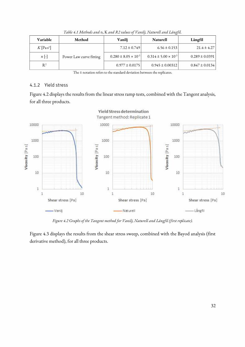
32

Table 4.1 Methods and n, K and R2 values of Vanilj, Naturell and Långfil.

Variable Method Vanilj Naturell Långfil

K [Pa∙sn]


7.12 ± 0.749 6.56 ± 0.153 21.4 ± 4.27

n [-] 0.280 ± 8.05 × 10-3 0.314 ± 5.00 × 10-3 0.289 ± 0.0391

R2 0.977 ± 0.0175 0.945 ± 0.00312 0.847 ± 0.0134

The ± notation refers to the standard deviation between the replicates.

4.1.2 Yield stress

Figure 4.2 displays the results from the linear stress ramp tests, combined with the Tangent analysis,

for all three products.

Figure 4.2 Graphs of the Tangent method for Vanilj, Naturell and Långfil (first replicate).

Figure 4.3 displays the results from the shear stress sweep, combined with the Bayod analysis (first

derivative method), for all three products.

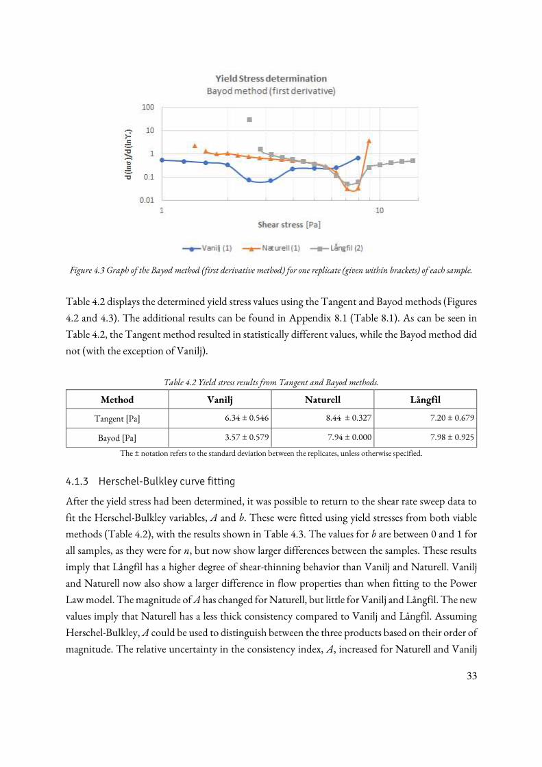
33

Figure 4.3 Graph of the Bayod method (first derivative method) for one replicate (given within brackets) of each sample.

Table 4.2 displays the determined yield stress values using the Tangent and Bayod methods (Figures

4.2 and 4.3). The additional results can be found in Appendix 8.1 (Table 8.1). As can be seen in

Table 4.2, the Tangent method resulted in statistically different values, while the Bayod method did

not (with the exception of Vanilj).

Table 4.2 Yield stress results from Tangent and Bayod methods.

Method Vanilj Naturell Långfil

Tangent [Pa] 6.34 ± 0.546 8.44 ± 0.327 7.20 ± 0.679

Bayod [Pa] 3.57 ± 0.579 7.94 ± 0.000 7.98 ± 0.925

The ± notation refers to the standard deviation between the replicates, unless otherwise specified.

4.1.3 Herschel-Bulkley curve fitting

After the yield stress had been determined, it was possible to return to the shear rate sweep data to

fit the Herschel-Bulkley variables, A and b. These were fitted using yield stresses from both viable

methods (Table 4.2), with the results shown in Table 4.3. The values for b are between 0 and 1 for

all samples, as they were for n, but now show larger differences between the samples. These results

imply that Långfil has a higher degree of shear-thinning behavior than Vanilj and Naturell. Vanilj

and Naturell now also show a larger difference in flow properties than when fitting to the Power

Law model. The magnitude of A has changed for Naturell, but little for Vanilj and Långfil. The new

values imply that Naturell has a less thick consistency compared to Vanilj and Långfil. Assuming

Herschel-Bulkley, A could be used to distinguish between the three products based on their order of

magnitude. The relative uncertainty in the consistency index, A, increased for Naturell and Vanilj

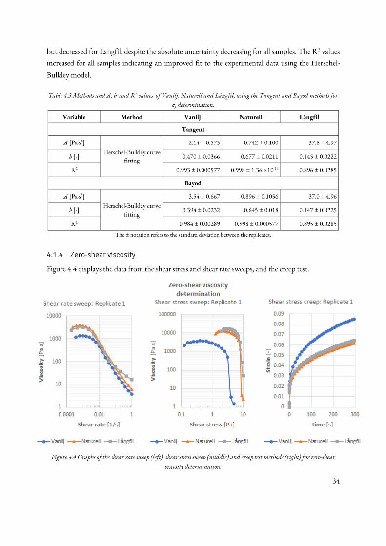
34

but decreased for Långfil, despite the absolute uncertainty decreasing for all samples. The R2 values

increased for all samples indicating an improved fit to the experimental data using the Herschel-

Bulkley model.

Table 4.3 Methods and A, b and R2 values of Vanilj, Naturell and Långfil, using the Tangent and Bayod methods for

σy determination.


Tangent

A [Pa∙sb]

Herschel-Bulkley curve fitting

2.14 ± 0.575 0.742 ± 0.100 37.8 ± 4.97

b [-] 0.470 ± 0.0366 0.677 ± 0.0211 0.145 ± 0.0222

R2 0.993 ± 0.000577 0.998 ± 1.36 ×10-16 0.896 ± 0.0285

Bayod

A [Pa∙sb]

Herschel-Bulkley curve fitting

3.54 ± 0.667 0.896 ± 0.1056 37.0 ± 4.96

b [-] 0.394 ± 0.0232 0.645 ± 0.018 0.147 ± 0.0225

R2 0.984 ± 0.00289 0.998 ± 0.000577 0.895 ± 0.0285



Figure 4.4 displays the data from the shear stress and shear rate sweeps, and the creep test.

Figure 4.4 Graphs of the shear rate sweep (left), shear stress sweep (middle) and creep test methods (right) for zero-shear

viscosity determination.

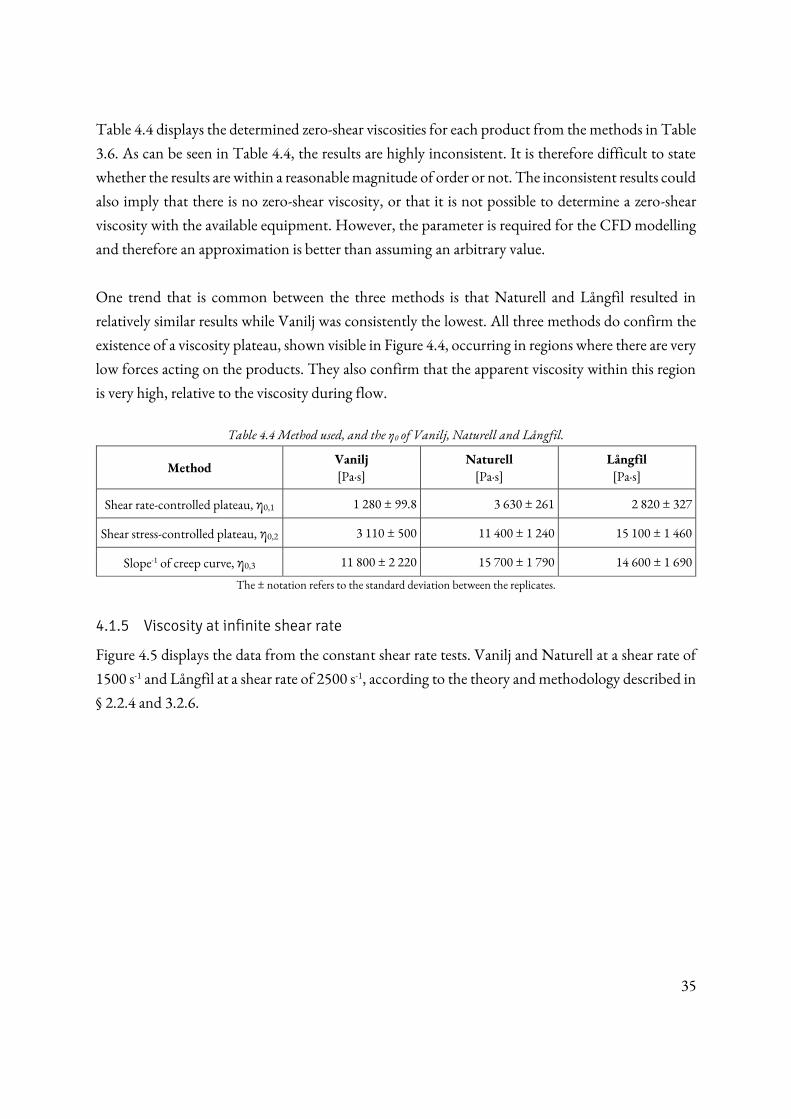
35

Table 4.4 displays the determined zero-shear viscosities for each product from the methods in Table

3.6. As can be seen in Table 4.4, the results are highly inconsistent. It is therefore difficult to state

whether the results are within a reasonable magnitude of order or not. The inconsistent results could

also imply that there is no zero-shear viscosity, or that it is not possible to determine a zero-shear

viscosity with the available equipment. However, the parameter is required for the CFD modelling

and therefore an approximation is better than assuming an arbitrary value.

One trend that is common between the three methods is that Naturell and Långfil resulted in

relatively similar results while Vanilj was consistently the lowest. All three methods do confirm the

existence of a viscosity plateau, shown visible in Figure 4.4, occurring in regions where there are very

low forces acting on the products. They also confirm that the apparent viscosity within this region

is very high, relative to the viscosity during flow.

Table 4.4 Method used, and the η0 of Vanilj, Naturell and Långfil.

Method Vanilj

[Pa∙s] Naturell

[Pa∙s] Långfil

[Pa∙s]

Shear rate-controlled plateau, η0,1 1 280 ± 99.8 3 630 ± 261 2 820 ± 327

Shear stress-controlled plateau, η0,2 3 110 ± 500 11 400 ± 1 240 15 100 ± 1 460

Slope-1 of creep curve, η0,3 11 800 ± 2 220 15 700 ± 1 790 14 600 ± 1 690



Figure 4.5 displays the data from the constant shear rate tests. Vanilj and Naturell at a shear rate of

1500 s-1 and Långfil at a shear rate of 2500 s-1, according to the theory and methodology described in

§ 2.2.4 and 3.2.6.

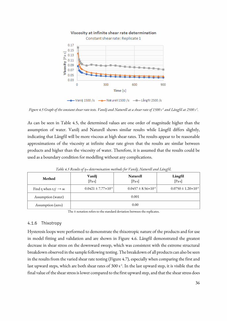
36

Figure 4.5 Graph of the constant shear rate tests. Vanilj and Naturell at a shear rate of 1500 s-1 and Långfil at 2500 s-1.

As can be seen in Table 4.5, the determined values are one order of magnitude higher than the

assumption of water. Vanilj and Naturell shows similar results while Långfil differs slightly,

indicating that Långfil will be more viscous at high shear rates. The results appear to be reasonable

approximations of the viscosity at infinite shear rate given that the results are similar between

products and higher than the viscosity of water. Therefore, it is assumed that the results could be

used as a boundary condition for modelling without any complications.

Table 4.5 Results of η∞ determination methods for Vanilj, Naturell and Långfil.

Method Vanilj

[Pa∙s] Naturell

[Pa∙s] Långfil

[Pa∙s]

Find η when t,γ ̇ → ∞ 0.0421 ± 7.77×10-4 0.0457 ± 8.56×10-4 0.0750 ± 1.20×10-4

Assumption (water) 0.001

Assumption (zero) 0.00


4.1.6 Thixotropy

Hysteresis loops were performed to demonstrate the thixotropic nature of the products and for use

in model fitting and validation and are shown in Figure 4.6. Långfil demonstrated the greatest

decrease in shear stress on the downward sweep, which was consistent with the extreme structural

breakdown observed in the sample following testing. The breakdown of all products can also be seen

in the results from the varied shear rate testing (Figure 4.7), especially when comparing the first and

last upward steps, which are both shear rates of 300 s-1. In the last upward step, it is visible that the

final value of the shear stress is lower compared to the first upward step, and that the shear stress does

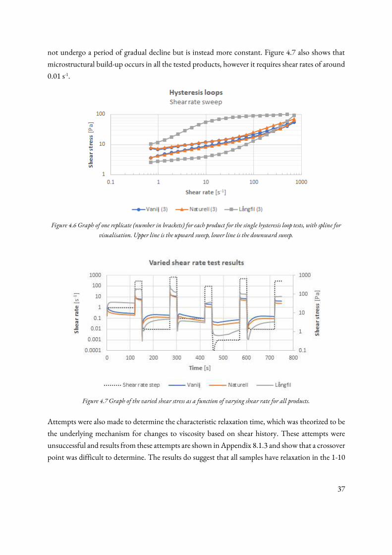
37

not undergo a period of gradual decline but is instead more constant. Figure 4.7 also shows that

microstructural build-up occurs in all the tested products, however it requires shear rates of around

0.01 s-1.

Figure 4.6 Graph of one replicate (number in brackets) for each product for the single hysteresis loop tests, with spline for

visualisation. Upper line is the upward sweep, lower line is the downward sweep.

Figure 4.7 Graph of the varied shear stress as a function of varying shear rate for all products.

Attempts were also made to determine the characteristic relaxation time, which was theorized to be

the underlying mechanism for changes to viscosity based on shear history. These attempts were

unsuccessful and results from these attempts are shown in Appendix 8.1.3 and show that a crossover

point was difficult to determine. The results do suggest that all samples have relaxation in the 1-10

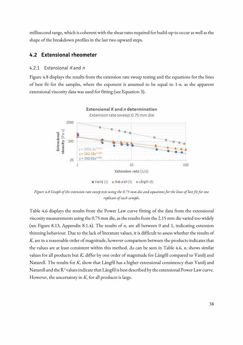
38

millisecond range, which is coherent with the shear rates required for build-up to occur as well as the

shape of the breakdown profiles in the last two upward steps.

4.2 Extensional rheometer

4.2.1 Extensional K and n

Figure 4.8 displays the results from the extension rate sweep testing and the equations for the lines

of best fit for the samples, where the exponent is assumed to be equal to 1-nε as the apparent

extensional viscosity data was used for fitting (see Equation 3).

Figure 4.8 Graph of the extension rate sweep tests using the 0.75 mm die and equations for the lines of best fit for one

replicate of each sample.

Table 4.6 displays the results from the Power Law curve fitting of the data from the extensional

viscosity measurements using the 0.75 mm die, as the results from the 2.15 mm die varied too widely

(see Figure 8.13, Appendix 8.1.4). The results of nε are all between 0 and 1, indicating extension

thinning behaviour. Due to the lack of literature values, it is difficult to assess whether the results of

Kε are in a reasonable order of magnitude, however comparison between the products indicates that

the values are at least consistent within this method. As can be seen in Table 4.6, nε shows similar

values for all products but Kε differ by one order of magnitude for Långfil compared to Vanilj and

Naturell. The results for Kε show that Långfil has a higher extensional consistency than Vanilj and

Naturell and the R2 values indicate that Långfil is best described by the extensional Power Law curve.

However, the uncertainty in Kε for all products is large.

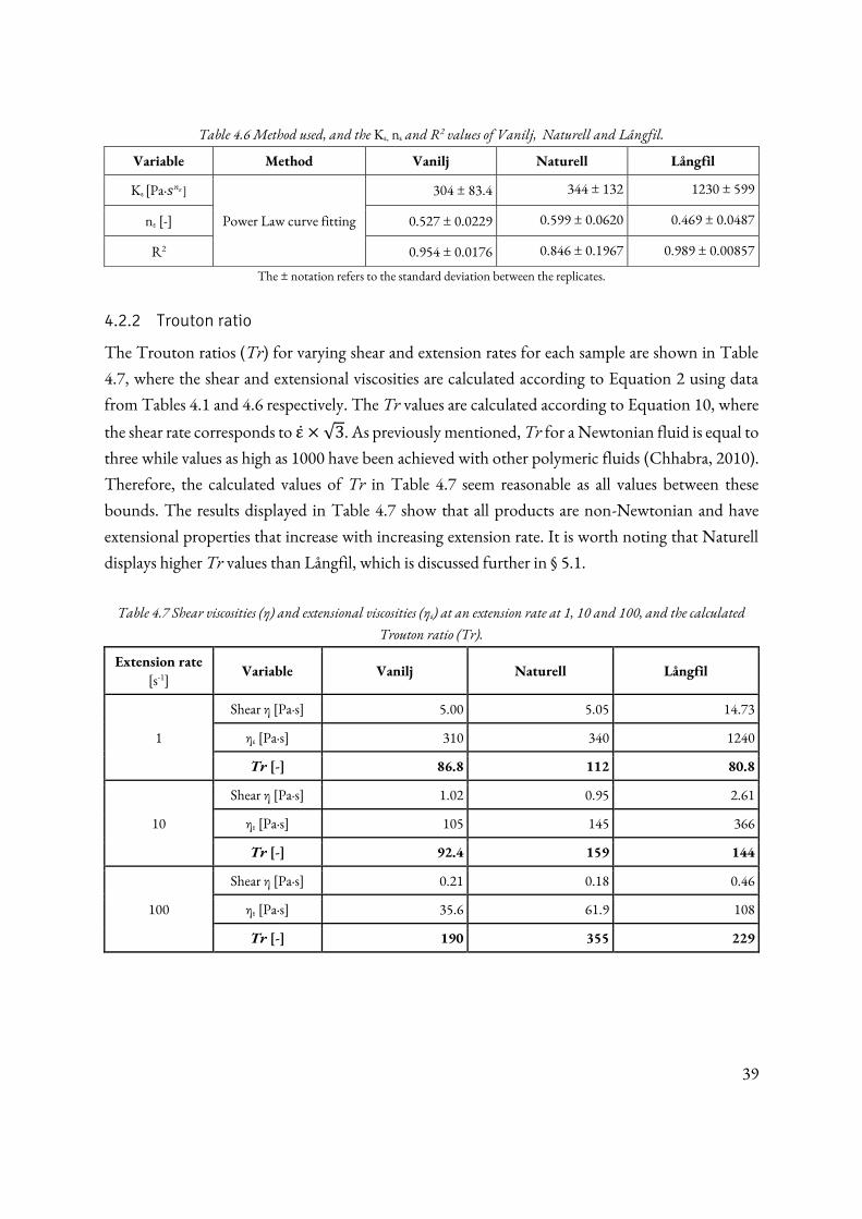
39

Table 4.6 Method used, and the Kε, nε and R2 values of Vanilj, Naturell and Långfil.


Kε [Pa∙𝑠𝑛𝜀 ]


304 ± 83.4 344 ± 132 1230 ± 599

nε [-] 0.527 ± 0.0229 0.599 ± 0.0620 0.469 ± 0.0487

R2 0.954 ± 0.0176 0.846 ± 0.1967 0.989 ± 0.00857


4.2.2 Trouton ratio

The Trouton ratios (Tr) for varying shear and extension rates for each sample are shown in Table

4.7, where the shear and extensional viscosities are calculated according to Equation 2 using data

from Tables 4.1 and 4.6 respectively. The Tr values are calculated according to Equation 10, where

the shear rate corresponds to ε̇ × √3. As previously mentioned, Tr for a Newtonian fluid is equal to

three while values as high as 1000 have been achieved with other polymeric fluids (Chhabra, 2010).

Therefore, the calculated values of Tr in Table 4.7 seem reasonable as all values between these

bounds. The results displayed in Table 4.7 show that all products are non-Newtonian and have

extensional properties that increase with increasing extension rate. It is worth noting that Naturell

displays higher Tr values than Långfil, which is discussed further in § 5.1.

Table 4.7 Shear viscosities (η) and extensional viscosities (ηε) at an extension rate at 1, 10 and 100, and the calculated

Trouton ratio (Tr).

Extension rate

[s-1] Variable Vanilj Naturell Långfil

1

Shear η [Pa∙s] 5.00 5.05 14.73

ηε [Pa∙s] 310 340 1240

Tr [-] 86.8 112 80.8

10

Shear η [Pa∙s] 1.02 0.95 2.61

ηε [Pa∙s] 105 145 366

Tr [-] 92.4 159 144

100

Shear η [Pa∙s] 0.21 0.18 0.46

ηε [Pa∙s] 35.6 61.9 108

Tr [-] 190 355 229

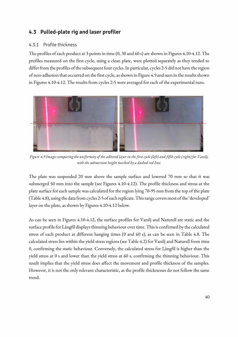
40

4.3 Pulled-plate rig and laser profiler

4.3.1 Profile thickness

The profiles of each product at 3 points in time (0, 30 and 60 s) are shown in Figures 4.10-4.12. The

profiles measured on the first cycle, using a clean plate, were plotted separately as they tended to

differ from the profiles of the subsequent four cycles. In particular, cycles 2-5 did not have the region

of non-adhesion that occurred on the first cycle, as shown in Figure 4.9 and seen in the results shown

in Figures 4.10-4.12. The results from cycles 2-5 were averaged for each of the experimental runs.

Figure 4.9 Images comparing the uniformity of the adhered layer in the first cycle (left) and fifth cycle (right) for Vanilj,

with the submersion height marked by a dashed red line.

The plate was suspended 20 mm above the sample surface and lowered 70 mm so that it was

submerged 50 mm into the sample (see Figures 4.10-4.12). The profile thickness and stress at the

plate surface for each sample was calculated for the region lying 70-95 mm from the top of the plate

(Table 4.8), using the data from cycles 2-5 of each replicate. This range covers most of the ‘developed’ layer on the plate, as shown by Figures 4.10-4.12 below.

As can be seen in Figures 4.10-4.12, the surface profiles for Vanilj and Naturell are static and the

surface profile for Långfil displays thinning behaviour over time. This is confirmed by the calculated

stress of each product at different hanging times (0 and 60 s), as can be seen in Table 4.8. The

calculated stress lies within the yield stress regions (see Table 4.2) for Vanilj and Naturell from time

0, confirming the static behaviour. Conversely, the calculated stress for Långfil is higher than the

yield stress at 0 s and lower than the yield stress at 60 s, confirming the thinning behaviour. This

result implies that the yield stress does affect the movement and profile thickness of the samples.

However, it is not the only relevant characteristic, as the profile thicknesses do not follow the same

trend.

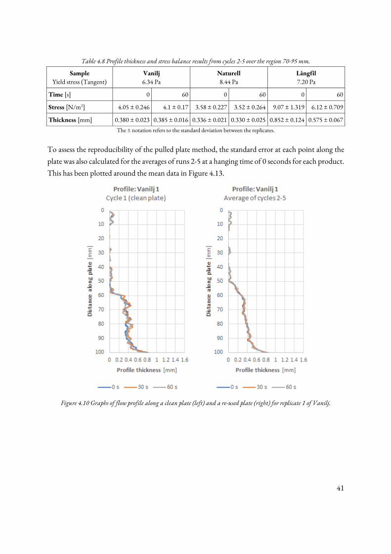
41

Table 4.8 Profile thickness and stress balance results from cycles 2-5 over the region 70-95 mm.

Sample

Yield stress (Tangent) Vanilj

6.34 Pa Naturell 8.44 Pa

Långfil 7.20 Pa

Time [s] 0 60 0 60 0 60

Stress [N/m2] 4.05 ± 0.246 4.1 ± 0.17 3.58 ± 0.227 3.52 ± 0.264 9.07 ± 1.319 6.12 ± 0.709

Thickness [mm] 0.380 ± 0.023 0.385 ± 0.016 0.336 ± 0.021 0.330 ± 0.025 0.852 ± 0.124 0.575 ± 0.067


To assess the reproducibility of the pulled plate method, the standard error at each point along the

plate was also calculated for the averages of runs 2-5 at a hanging time of 0 seconds for each product.

This has been plotted around the mean data in Figure 4.13.

Figure 4.10 Graphs of flow profile along a clean plate (left) and a re-used plate (right) for replicate 1 of Vanilj.

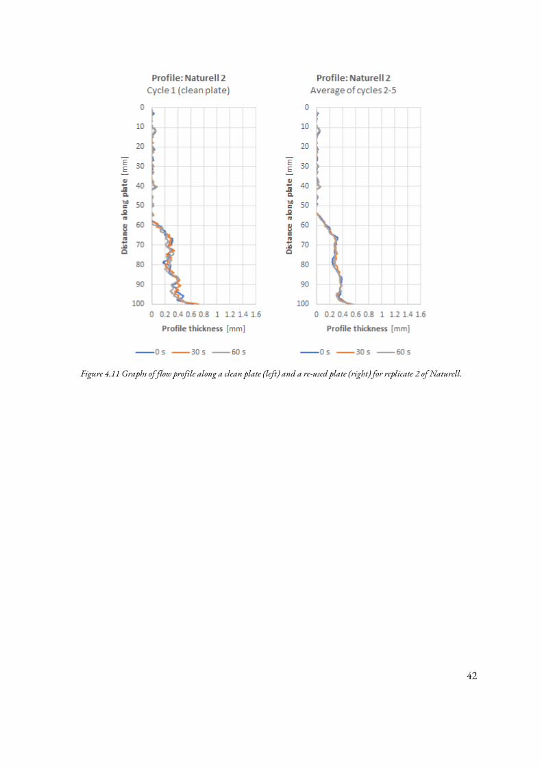
42

Figure 4.11 Graphs of flow profile along a clean plate (left) and a re-used plate (right) for replicate 2 of Naturell.

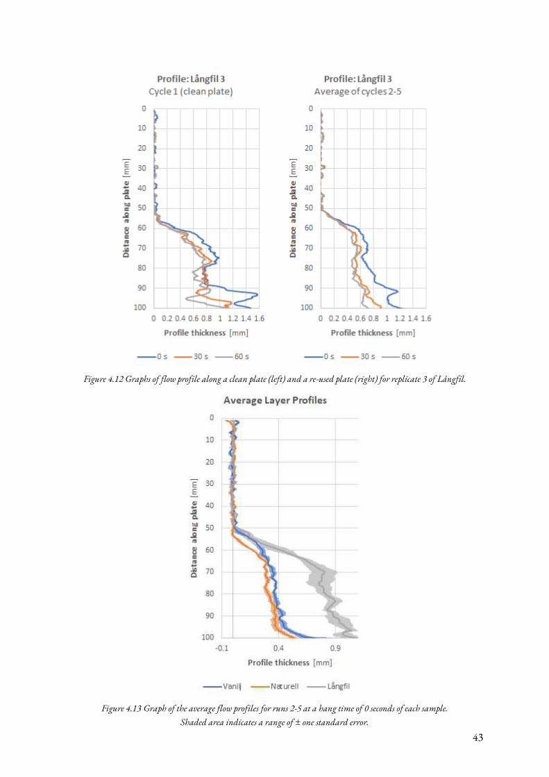
43

Figure 4.12 Graphs of flow profile along a clean plate (left) and a re-used plate (right) for replicate 3 of Långfil.

Figure 4.13 Graph of the average flow profiles for runs 2-5 at a hang time of 0 seconds of each sample.

Shaded area indicates a range of ± one standard error.

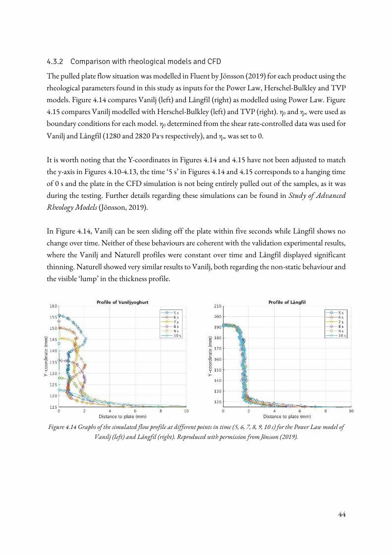
44

4.3.2 Comparison with rheological models and CFD

The pulled plate flow situation was modelled in Fluent by Jönsson (2019) for each product using the

rheological parameters found in this study as inputs for the Power Law, Herschel-Bulkley and TVP

models. Figure 4.14 compares Vanilj (left) and Långfil (right) as modelled using Power Law. Figure

4.15 compares Vanilj modelled with Herschel-Bulkley (left) and TVP (right). η0 and η∞ were used as

boundary conditions for each model. η0 determined from the shear rate-controlled data was used for

Vanilj and Långfil (1280 and 2820 Paᐧs respectively), and η∞ was set to 0.

It is worth noting that the Y-coordinates in Figures 4.14 and 4.15 have not been adjusted to match

the y-axis in Figures 4.10-4.13, the time ‘5 s’ in Figures 4.14 and 4.15 corresponds to a hanging time of 0 s and the plate in the CFD simulation is not being entirely pulled out of the samples, as it was

during the testing. Further details regarding these simulations can be found in Study of Advanced

Rheology Models (Jönsson, 2019).

In Figure 4.14, Vanilj can be seen sliding off the plate within five seconds while Långfil shows no

change over time. Neither of these behaviours are coherent with the validation experimental results,

where the Vanilj and Naturell profiles were constant over time and Långfil displayed significant

thinning. Naturell showed very similar results to Vanilj, both regarding the non-static behaviour and

the visible ‘lump’ in the thickness profile.

Figure 4.14 Graphs of the simulated flow profile at different points in time (5, 6, 7, 8, 9, 10 s) for the Power Law model of

Vanilj (left) and Långfil (right). Reproduced with permission from Jönsson (2019).

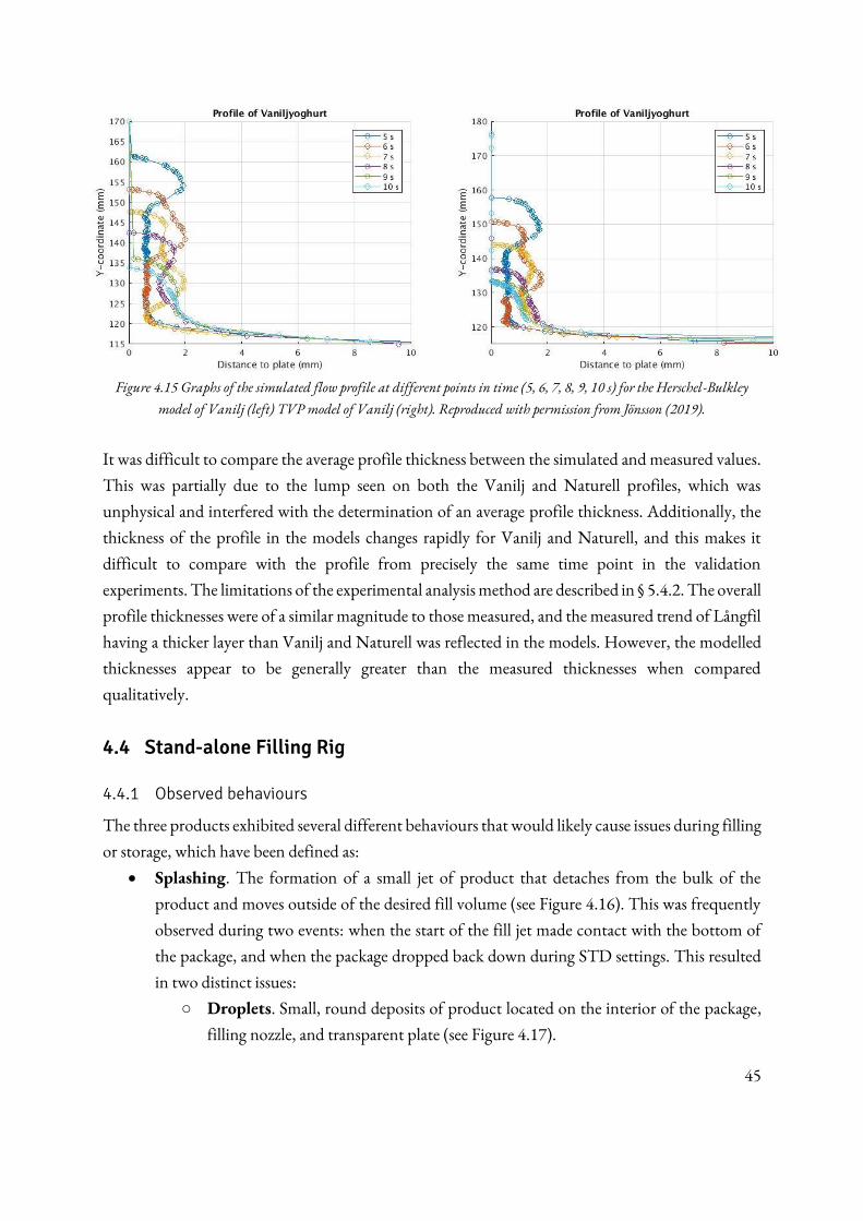
45

Figure 4.15 Graphs of the simulated flow profile at different points in time (5, 6, 7, 8, 9, 10 s) for the Herschel-Bulkley

model of Vanilj (left) TVP model of Vanilj (right). Reproduced with permission from Jönsson (2019).

It was difficult to compare the average profile thickness between the simulated and measured values.

This was partially due to the lump seen on both the Vanilj and Naturell profiles, which was

unphysical and interfered with the determination of an average profile thickness. Additionally, the

thickness of the profile in the models changes rapidly for Vanilj and Naturell, and this makes it

difficult to compare with the profile from precisely the same time point in the validation

experiments. The limitations of the experimental analysis method are described in § 5.4.2. The overall

profile thicknesses were of a similar magnitude to those measured, and the measured trend of Långfil

having a thicker layer than Vanilj and Naturell was reflected in the models. However, the modelled

thicknesses appear to be generally greater than the measured thicknesses when compared

qualitatively.

4.4 Stand-alone Filling Rig

4.4.1 Observed behaviours

The three products exhibited several different behaviours that would likely cause issues during filling

or storage, which have been defined as:

• Splashing. The formation of a small jet of product that detaches from the bulk of the

product and moves outside of the desired fill volume (see Figure 4.16). This was frequently

observed during two events: when the start of the fill jet made contact with the bottom of

the package, and when the package dropped back down during STD settings. This resulted

in two distinct issues:

○ Droplets. Small, round deposits of product located on the interior of the package,

filling nozzle, and transparent plate (see Figure 4.17).

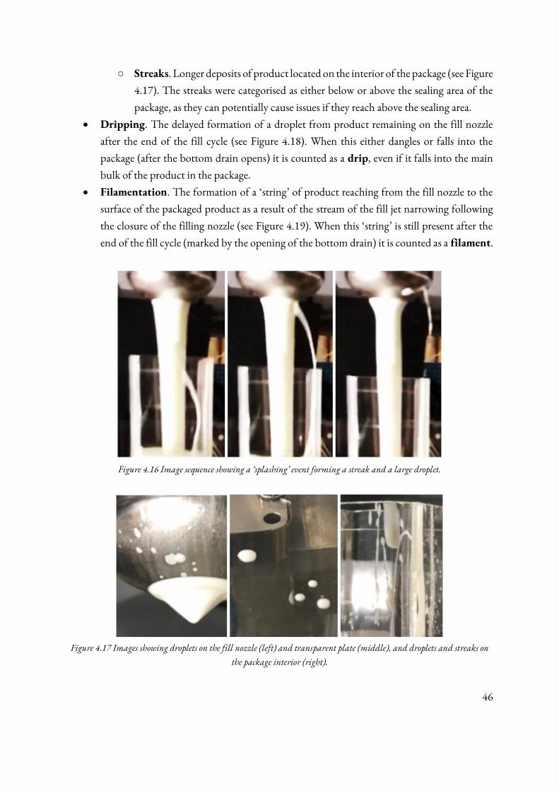
46

○ Streaks. Longer deposits of product located on the interior of the package (see Figure

4.17). The streaks were categorised as either below or above the sealing area of the

package, as they can potentially cause issues if they reach above the sealing area.

• Dripping. The delayed formation of a droplet from product remaining on the fill nozzle

after the end of the fill cycle (see Figure 4.18). When this either dangles or falls into the

package (after the bottom drain opens) it is counted as a drip, even if it falls into the main

bulk of the product in the package.

• Filamentation. The formation of a ‘string’ of product reaching from the fill nozzle to the surface of the packaged product as a result of the stream of the fill jet narrowing following

the closure of the filling nozzle (see Figure 4.19). When this ‘string’ is still present after the end of the fill cycle (marked by the opening of the bottom drain) it is counted as a filament.

Figure 4.16 Image sequence showing a ‘splashing’ event forming a streak and a large droplet.

Figure 4.17 Images showing droplets on the fill nozzle (left) and transparent plate (middle), and droplets and streaks on

the package interior (right).

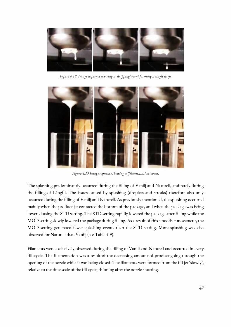
47

Figure 4.18 Image sequence showing a ‘dripping’ event forming a single drip.

Figure 4.19 Image sequence showing a ‘filamentation’ event.

The splashing predominantly occurred during the filling of Vanilj and Naturell, and rarely during

the filling of Långfil. The issues caused by splashing (droplets and streaks) therefore also only

occurred during the filling of Vanilj and Naturell. As previously mentioned, the splashing occurred

mainly when the product jet contacted the bottom of the package, and when the package was being

lowered using the STD setting. The STD setting rapidly lowered the package after filling while the

MOD setting slowly lowered the package during filling. As a result of this smoother movement, the

MOD setting generated fewer splashing events than the STD setting. More splashing was also

observed for Naturell than Vanilj (see Table 4.9).

Filaments were exclusively observed during the filling of Vanilj and Naturell and occurred in every

fill cycle. The filamentation was a result of the decreasing amount of product going through the

opening of the nozzle while it was being closed. The filaments were formed from the fill jet ‘slowly’, relative to the time scale of the fill cycle, thinning after the nozzle shutting.

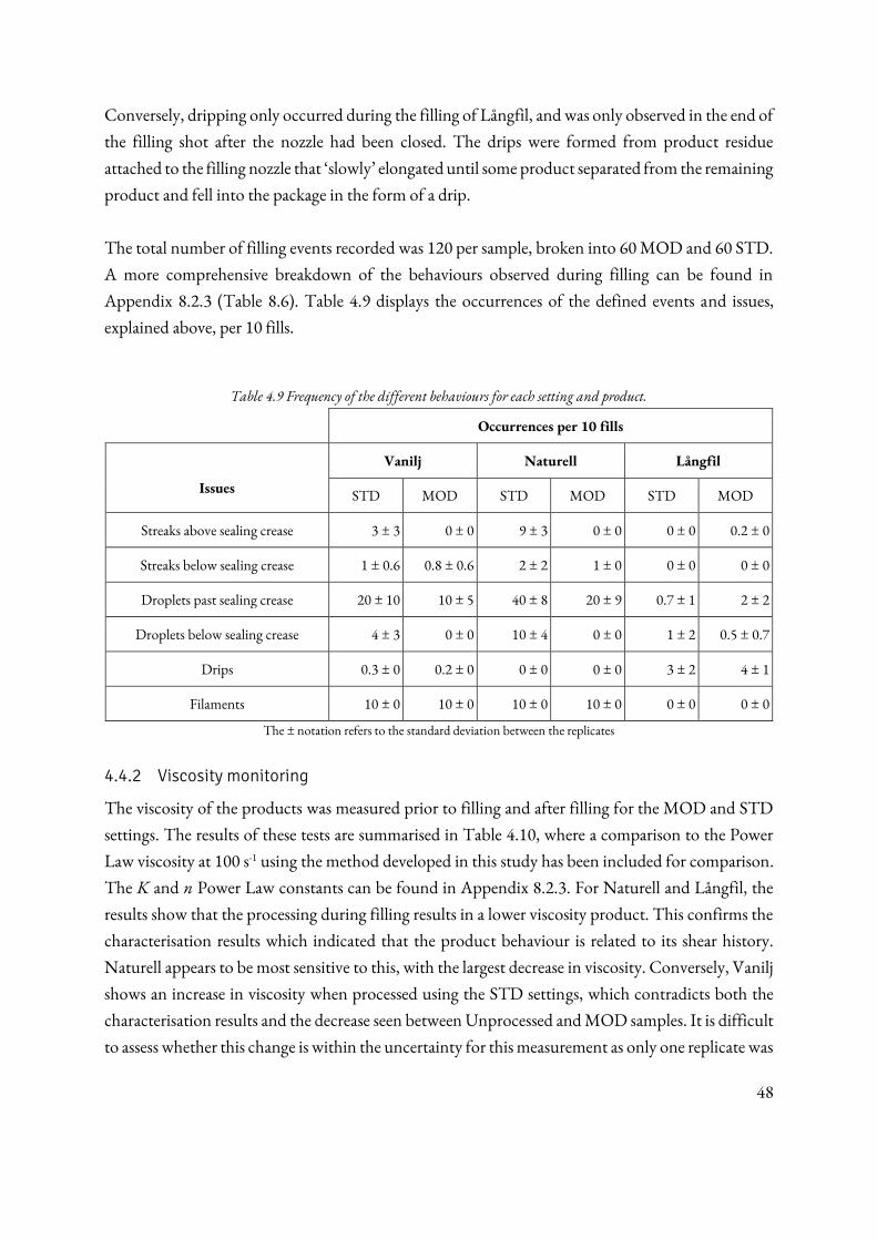
48

Conversely, dripping only occurred during the filling of Långfil, and was only observed in the end of

the filling shot after the nozzle had been closed. The drips were formed from product residue

attached to the filling nozzle that ‘slowly’ elongated until some product separated from the remaining product and fell into the package in the form of a drip.

The total number of filling events recorded was 120 per sample, broken into 60 MOD and 60 STD.

A more comprehensive breakdown of the behaviours observed during filling can be found in

Appendix 8.2.3 (Table 8.6). Table 4.9 displays the occurrences of the defined events and issues,

explained above, per 10 fills.

Table 4.9 Frequency of the different behaviours for each setting and product.

Occurrences per 10 fills

Issues

Vanilj Naturell Långfil

STD MOD STD MOD STD MOD

Streaks above sealing crease 3 ± 3 0 ± 0 9 ± 3 0 ± 0 0 ± 0 0.2 ± 0

Streaks below sealing crease 1 ± 0.6 0.8 ± 0.6 2 ± 2 1 ± 0 0 ± 0 0 ± 0

Droplets past sealing crease 20 ± 10 10 ± 5 40 ± 8 20 ± 9 0.7 ± 1 2 ± 2

Droplets below sealing crease 4 ± 3 0 ± 0 10 ± 4 0 ± 0 1 ± 2 0.5 ± 0.7

Drips 0.3 ± 0 0.2 ± 0 0 ± 0 0 ± 0 3 ± 2 4 ± 1

Filaments 10 ± 0 10 ± 0 10 ± 0 10 ± 0 0 ± 0 0 ± 0

The ± notation refers to the standard deviation between the replicates

4.4.2 Viscosity monitoring

The viscosity of the products was measured prior to filling and after filling for the MOD and STD

settings. The results of these tests are summarised in Table 4.10, where a comparison to the Power

Law viscosity at 100 s-1 using the method developed in this study has been included for comparison.

The K and n Power Law constants can be found in Appendix 8.2.3. For Naturell and Långfil, the

results show that the processing during filling results in a lower viscosity product. This confirms the

characterisation results which indicated that the product behaviour is related to its shear history.

Naturell appears to be most sensitive to this, with the largest decrease in viscosity. Conversely, Vanilj

shows an increase in viscosity when processed using the STD settings, which contradicts both the

characterisation results and the decrease seen between Unprocessed and MOD samples. It is difficult

to assess whether this change is within the uncertainty for this measurement as only one replicate was

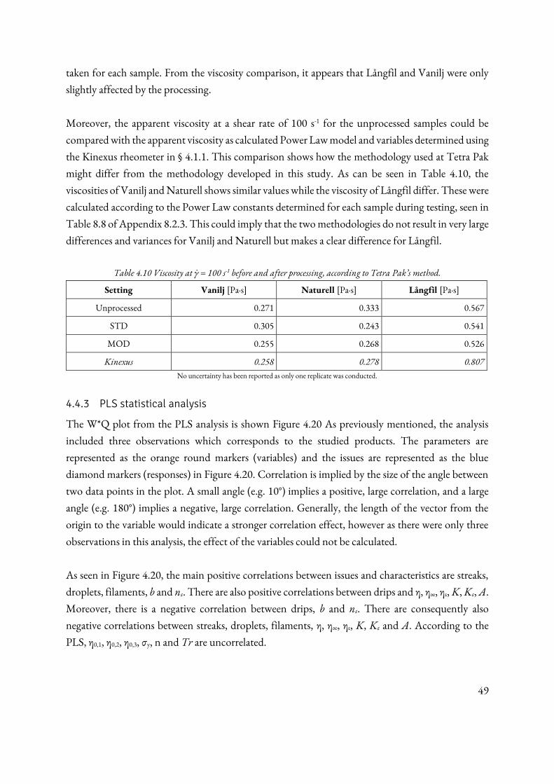
49

taken for each sample. From the viscosity comparison, it appears that Långfil and Vanilj were only

slightly affected by the processing.

Moreover, the apparent viscosity at a shear rate of 100 s-1 for the unprocessed samples could be

compared with the apparent viscosity as calculated Power Law model and variables determined using

the Kinexus rheometer in § 4.1.1. This comparison shows how the methodology used at Tetra Pak

might differ from the methodology developed in this study. As can be seen in Table 4.10, the

viscosities of Vanilj and Naturell shows similar values while the viscosity of Långfil differ. These were

calculated according to the Power Law constants determined for each sample during testing, seen in

Table 8.8 of Appendix 8.2.3. This could imply that the two methodologies do not result in very large

differences and variances for Vanilj and Naturell but makes a clear difference for Långfil.

Table 4.10 Viscosity at γ̇ = 100 s-1 before and after processing, according to Tetra Pak’s method.

Setting Vanilj [Pa∙s] Naturell [Pa∙s] Långfil [Pa∙s]

Unprocessed 0.271 0.333 0.567

STD 0.305 0.243 0.541

MOD 0.255 0.268 0.526

Kinexus 0.258 0.278 0.807

No uncertainty has been reported as only one replicate was conducted.

4.4.3 PLS statistical analysis

The W*Q plot from the PLS analysis is shown Figure 4.20 As previously mentioned, the analysis

included three observations which corresponds to the studied products. The parameters are

represented as the orange round markers (variables) and the issues are represented as the blue

diamond markers (responses) in Figure 4.20. Correlation is implied by the size of the angle between

two data points in the plot. A small angle (e.g. 10°) implies a positive, large correlation, and a large

angle (e.g. 180°) implies a negative, large correlation. Generally, the length of the vector from the

origin to the variable would indicate a stronger correlation effect, however as there were only three

observations in this analysis, the effect of the variables could not be calculated.

As seen in Figure 4.20, the main positive correlations between issues and characteristics are streaks,

droplets, filaments, b and nε. There are also positive correlations between drips and η, η∞, ηε, K, Kε, A.

Moreover, there is a negative correlation between drips, b and nε. There are consequently also

negative correlations between streaks, droplets, filaments, η, η∞, ηε, K, Kε and A. According to the

PLS, η0,1, η0,2, η0,3, σy, n and Tr are uncorrelated.

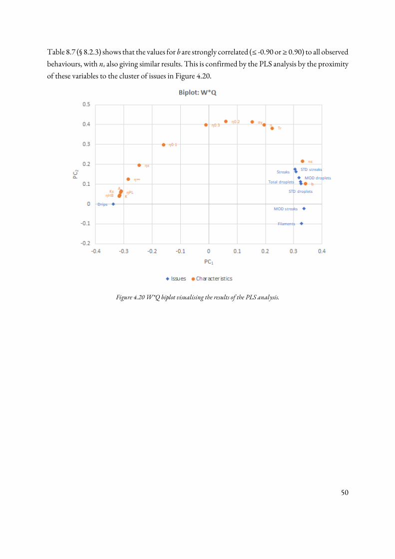
50

Table 8.7 (§ 8.2.3) shows that the values for b are strongly correlated (≤ -0.90 or ≥ 0.90) to all observed behaviours, with nε also giving similar results. This is confirmed by the PLS analysis by the proximity

of these variables to the cluster of issues in Figure 4.20.

Figure 4.20 W*Q biplot visualising the results of the PLS analysis.

51

5 Discussion

5.1 Characterisation methods and parameters

The characterisation parameters and their determination methods were evaluated with regard to their

applicability in describing the products and the reproducibility of the results, as indicated by the

maximum relative standard error (RSE) among the products. The shear K and n values were

determined from shear rate sweep data and successfully yielded reproducible results (RSE <6 % and

<2% respectively) for Vanilj and Naturell, with Långfil displaying greater variance (RSE <12 % and

<8%). The results also showed a reasonable fit to the experimental data, as shown by the R2 values.

The results are similar to results obtained with the method used at Tetra Pak in both their magnitude

and the trends shown between the product. This confirms that the K and n results obtained in this

study are reasonable. K showed a statistical difference between the yoghurt samples compared to

Långfil, but not between the yoghurt samples. This implies that K could potentially distinguish

between yoghurts and Långfil, which appears to be supported by the PLS analysis showing negative

correlation with streaks and filaments, and positive correlation with drips.

The yield stress values depend strongly on the determination method. However, the yield stress

results were similar between all products, regardless of the method used. The Second derivative

method was only applied to a single replicate for each product, due to difficulties in calculation in

this study, however the results closely resemble those of the Tangent method as applied to the same

data. The Mendes & Dutra method was based on shear rate-controlled data, which is less reliable

than shear stress-controlled data as the measured shear stresses may overlap in shear rate-controlled

tests (Tornberg, 2019). The Maximum viscosity method is believed to be the least reliable since this

analysis method resulted in a broad region of high viscosity, making it difficult to locate the

maximum viscosity. The Tangent method using SAOS data gave less reproducible results (RSE <10

%), as calculated from the standard deviations. The Tangent method applied to shear stress-

controlled data showed greatest agreement with other methods (Bayod and Second derivative) while

also producing reproducible (RSE <5 %) and statistically different results between products. The

linear stress ramp measurement method combined with the Tangent analysis method is therefore

recommended for the determination of σy.

Even larger differences were observed between products when σy was used for the fitting of the

Herschel-Bulkley constants, A and b, to the same shear rate sweep data used to determine K and n.

This reflects the qualitative differences between the products that are experienced when consuming

the products. This was an interesting result, and indicates that σy, A and b could be better used for

characterisation and to distinguish between the studied products. Additionally, A and b improved

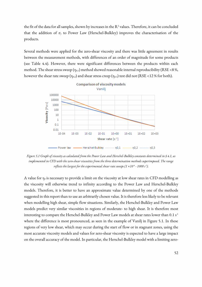
52

the fit of the data for all samples, shown by increases in the R2 values. Therefore, it can be concluded

that the addition of σy to Power Law (Herschel-Bulkley) improves the characterisation of the

products.

Several methods were applied for the zero-shear viscosity and there was little agreement in results

between the measurement methods, with differences of an order of magnitude for some products

(see Table 4.4). However, there were significant differences between the products within each

method. The shear stress sweep (η0,1) method showed reasonable internal reproducibility (RSE <8 %,

however the shear rate sweep (η0,2) and shear stress creep (η0,3) test did not (RSE <12 % for both).

Figure 5.1 Graph of viscosity as calculated from the Power Law and Herschel-Bulkley constants determined in § 4.1, as

implemented in CFD with the zero-shear viscosities from the three determination methods superimposed. The range

reflects the largest for the experimental shear rate sweeps (1 ×10-4 - 1000 s-1).

A value for η0 is necessary to provide a limit on the viscosity at low shear rates in CFD modelling as

the viscosity will otherwise trend to infinity according to the Power Law and Herschel-Bulkley

models. Therefore, it is better to have an approximate value determined by one of the methods

suggested in this report than to use an arbitrarily chosen value. It is therefore less likely to be relevant

when modelling high shear, simple flow situations. Similarly, the Herschel-Bulkley and Power Law

models predict very similar viscosities in regions of moderate- to high shear. It is therefore most

interesting to compare the Herschel-Bulkley and Power Law models at shear rates lower than 0.1 s-1

where the difference is most pronounced, as seen in the example of Vanilj in Figure 5.1. In these

regions of very low shear, which may occur during the start of flow or in stagnant zones, using the

most accurate viscosity models and values for zero-shear viscosity is expected to have a large impact

on the overall accuracy of the model. In particular, the Herschel-Bulkley model with a limiting zero-

53

shear viscosity would predict that a constant viscosity is maintained by the fluid until the shear rate

increases approximately an order of magnitude above that of the Power Law.

As previously mentioned, the Cross analysis for determining viscosity at infinite shear rate could not

be performed due to the limitations of the available equipment, and therefore a cruder method was

developed to approximate the value. In the method developed for this study, there was a statistical

difference between the products, with Långfil showing the highest η. This may be explained by

Långfil containing longer polysaccharide chains than the yoghurt products, resulting in the

microstructure of Långfil taking longer time to breakdown. However, two key limitations of this

method were the test duration and shear rates. The test duration was limited to 15 minutes, as steady

state behaviour cannot be reached within 60 minutes for yoghurts. The shear rates were limited by

the turbulence occurring at higher shear rates. The general similarity between products was expected,

since it was assumed that η∞ would approach the viscosity of water (10-3 Paᐧs) for all samples as shear

rate and time approaches infinity. Despite the PLS analysis indicating that η∞ is correlated to some of

the filling issues, the results of this study suggest that η as calculated from using Power Law or

Herschel-Bulkley models is a better indicator. Additionally, the CFD modelling was able to function

with the assumption that η∞ is 0 Paᐧs, even if this is highly unrealistic. Therefore, performing testing

to determine η∞ does not contribute to the understanding, modelling or prediction of the product

and its behaviour.

As expected from its observably ‘stretchy’ flow behaviour, Långfil yielded a significantly different Kε

and nε values compared to Vanilj and Naturell, and a higher overall ηε. This did however not match

with the expected outcome of the calculated Trouton ratio. Since the Tr = 3 for Newtonian fluids,

it was expected that Tr >> 3 for the studied products. While this was confirmed, with Tr > 80 for all

samples, the Tr was unexpectedly higher for Naturell than Långfil. Without applying more

systematic variation to the composition of the tested samples it is difficult to attribute this outcome

to actual differences in the samples, errors in methodology or flaws in the experimental theory. It

could, for example, be due to the contribution of shear stress and shear rate to the apparent

extensional viscosity. From this it can be concluded, that the measurement method for extensional

viscosity, which yields ηε, Kε and nε, can be used for distinguishing between the products when

comparing results within the method, but not with results from other methods.

5.2 Comparison of behaviour indicators

The results of the exploratory study conducted in this work indicates that it is possible to correlate

the observed events and issues during filling to the determined rheological parameters (see Figure

4.19). As previously mentioned, the PLS analysis only included three observations (Vanilj, Naturell

54

and Långfil). Therefore, it was not possible to estimate the magnitude of the effect of the variables

on the responses. The result of the statistical analysis can however still be used as an early indication

of which rheological parameters that could be chosen for further studying.

From Figure 4.19 it is possible to see that the parameters b and nε are positively correlated to all

observed issues except ‘drips’, and negatively correlated to ‘drips’. This is reasonable since both b and

nε are variables related to the flow properties of the products. It also suggests that the parameters b

and nε are of interest for future work aiming to predict all filling issues. Since b is determined from

the Herschel-Bulkley model, the determination of σy would therefore be necessary for future work,

even though σy did not show any strong correlation to any of the observed issues in isolation.

Zero-shear viscosity and Trouton ratio did not show any strong correlation to any of the observed

issues. This is coherent with the unexpected result of the Tr and the unreliable results from the η0

determination. This suggests that η0 and Tr are rheological parameters that are not of very high

relevance for the prediction of issues during filling for the studied products, even if the values of η0

are required as boundary conditions for CFD modelling.

ηε, η∞, η (both from Power Law and Herschel-Bulkley), A, K and Kε appear to all be positively

correlated to ‘drips’ and negatively correlated to most of the other observed issues. This is also a result that would appear to be reasonable in context of § 4.1, where it was discussed that the consistency

indices (A, K and Kε) were the rheological parameters that could most clearly distinguish Långfil from

the yoghurt samples. Similarly, ‘dripping’ was only observed in Långfil and never in the yoghurt

samples.

With respect to ease of measurement, availability of equipment and strength of correlation to filling

issues, this study indicates that the Tangent method for σy analysis and corresponding Herschel-

Bulkley coefficients, A and b, are most worthwhile to investigate further.

5.3 Evaluation of validation methods

The two validation methods used in this work were chosen with the aim of producing results that

could be used for validating the rheological models and identifying behaviour indicators. This section

will evaluate the success of these methods in achieving these goals.

5.3.1 Pulled plate method

The pulled plate experiments were successfully able to measure the profile of yoghurt as it adhered

to the surface of a metal plate, with a measurement precision of ± 0.1 mm. The results were

55

successfully reproduced in 6 separate trials for each product, with cycles 2-5 (unclean plate) having

minimal overlap between the products (being seen in Figure 4.13). This indicates that a multiple-

cycle pulled plate method can be reliably used to visualise and measure the surface profile thickness

of fermented dairy products.

There were clear differences in the flow behaviours of the different products. The Vanilj and Naturell

products showed very little change with respect to time, while Långfil showed thinning of the

adhered layer. The initial thickness of the adhered layer was greatest in Långfil although the final

thickness was similar to that of Vanilj and Naturell. Flow down the plate was suggested in several

Långfil replicates where ‘lumps’ could be seen (Figures 4.10-4.12) moving downwards at the

different time points. The relevance of the yield stress in these tests was confirmed by the thinning

of the Långfil profile over time. This implies that the yield stress determines an upper limit on the

thickness of the adhered layer but will not determine how thick the layer is below this limit. This

indicates that there are parameters other than yield stress contributing to the shape and thickness of

the surface profile of the studied products in this method.

The purpose of visualising of the sample profile at different points in time was to compare the

empirical data to data simulated with different rheological models in a CFD framework (Fluent). As

mentioned in § 4.3.2, the CFD simulations contradict the empirical data. It was therefore difficult to

compare the CFD results to the experimental data and draw conclusions regarding which rheological

model best describes the dynamic behaviour of the studied products. As can be seen in Figures 4.14

and 4.15, none of the models (Power Law, Herschel-Bulkley and TVP) managed to successfully

simulate results that reflects reality. This may indicate that the pulled plate validation method is

unsuitable for validating modelling in simple flow situations. However, the presence of unlikely

behaviour in the modelling results, such as lumps in the Vanilj and Naturell products, indicate that

the issues may be related to the models or the parameters used in them.

Overall, this method was simple to execute experimentally but could benefit from refinement as it

required labor intensive analysis with a wide margin for human error in the interpretation of the

results (see § 3.4.4).

5.3.2 Filling rig method

Validation testing in the filling rig aimed to reveal if different filling issues occurred more frequently

in some products than others. The experiment was successful in showing clear differences in

behaviour between all three sample types under the same filling conditions. The operating conditions

56

resulted in enough filling issues for the target issues to be identified and quantified, but not so many

that it became difficult to distinguish individual issues.

One concern was that the three samples would behave very similarly during filling, despite their

noticeable differences in everyday use. Långfil was included in this study for the purpose of

confirming if this occurred. Fortunately, the yoghurt samples mainly displayed issues with splashing

while Långfil mainly displayed dripping, as shown in Table 4.9. This clear difference in behaviour

indicates that the differences in product characteristics are also reflected during filling, using either

the MOD or the STD settings.

The correlation between the characteristics and the behaviours was limited by the number of

products (in PLS defined as observations) used during testing, which prevented further analysis into

the strength of the correlations through methods such as PLS. This was due to the number of

responses exceeding the number of observations which resulted in negative degrees of freedom.

However, the results from this exploratory study were still able to show that there is potential for

developing behaviour indicators and possibly numerical relationships to predict fill behaviour. The

correlation of the b and nε suggest that the flow characteristics of the products may affect filling. The

methods used for determining and correlating these characteristics can be used to further investigate

their applicability.

5.4 Experimental uncertainty and error

5.4.1 Limitations of methodology

The overarching methodology employed in this work was the comparison of three fermented dairy

products with variations in fat content, culture, and stabilisers. They were also purchased from

conventional retailers rather than prepared specifically for the project. Overall, this introduced

numerous unknown variables, making it difficult to precisely correlate the measured characteristics

and filling behaviour to yoghurt composition. This could have been improved upon by selecting two

products (e.g. Naturell and Långfil) and using these to create samples of varying concentrations.

Producing the fermented dairy products from raw ingredients under highly controlled conditions

would also reduce the variability of the tests, and is a method commonly employed to reduce sample

variability (Skriver et al., 1993; Guénard-Lampron et al., 2018).

The extensional viscosity measurements assume that the products have a shear viscosity that can be

described by Power Law, but this assumption was not confirmed in the characterisation phase. It can

be debated whether the method is successful in its assumptions and calculations, and therefore

57

whether a ‘true’ extensional viscosity could be determined. However, the current method is sufficient

for use as a behaviour indicator.

The comparison of K and n determination results with measurements using Tetra Pak’s existing methods and instruments showed reasonable agreement. Further comparison with existing

characterisation methodologies at Tetra Pak could be beneficial for the evaluation of the

methodologies developed in this study.

The geometry available for the rotational rheometer may not have been ideal, especially for the

determination of the yield stress, characteristic relaxation time and viscosity at infinite shear rate. The

use of plate-plate geometry would have disturbed the samples less during loading, and this may have

resulted more valid yield stress and relaxation time measurements. A smaller gap in the cup-and-bob

geometry may have prevented the development of turbulence during the η∞ measurements, allowing

the tests to be conducted at higher shear rates.

A general limitation for all sweep tests was the stabilisation time, which limited the number of data

points that could be collected. A compromise had to be reached between measuring sufficiently

many data points and the overall length of time required for test. Given that each data point required

a stabilisation time of 40-90 seconds, limitations were placed on either the number of decades

measured or the samples per decade needed. This led to errors in some methodologies, such as the

Bayod yield stress determination, which are discussed in § 5.4.3.

5.4.2 Uncertainty and reliability

The sample handling technique, which included homogenisation, pre-shearing and resting time, was

evaluated with respect to the reproducibility of the results. To attempt to capture the time dependent

effects of the yoghurt, it was decided early on that no pre-shearing should be applied to the products

before performing the measurements. The sample was also only left to rest for 60 seconds in the

geometry before starting the measurement. The duration of the resting time may contribute to, or

reduce, measurement uncertainties depending on how fast the product structure rebuilds itself.

However, it was decided that a resting time was not of interest in this project due to the aim of

characterising the dairy products during filling, when the product is heavily sheared and have very

little time to rebuild itself. The results from the measurements performed during the characterisation

phase showed high reproducibility even though no calibration was performed on the used

equipment. This indicates that the sampling handling technique developed in this project produces

reliable results.

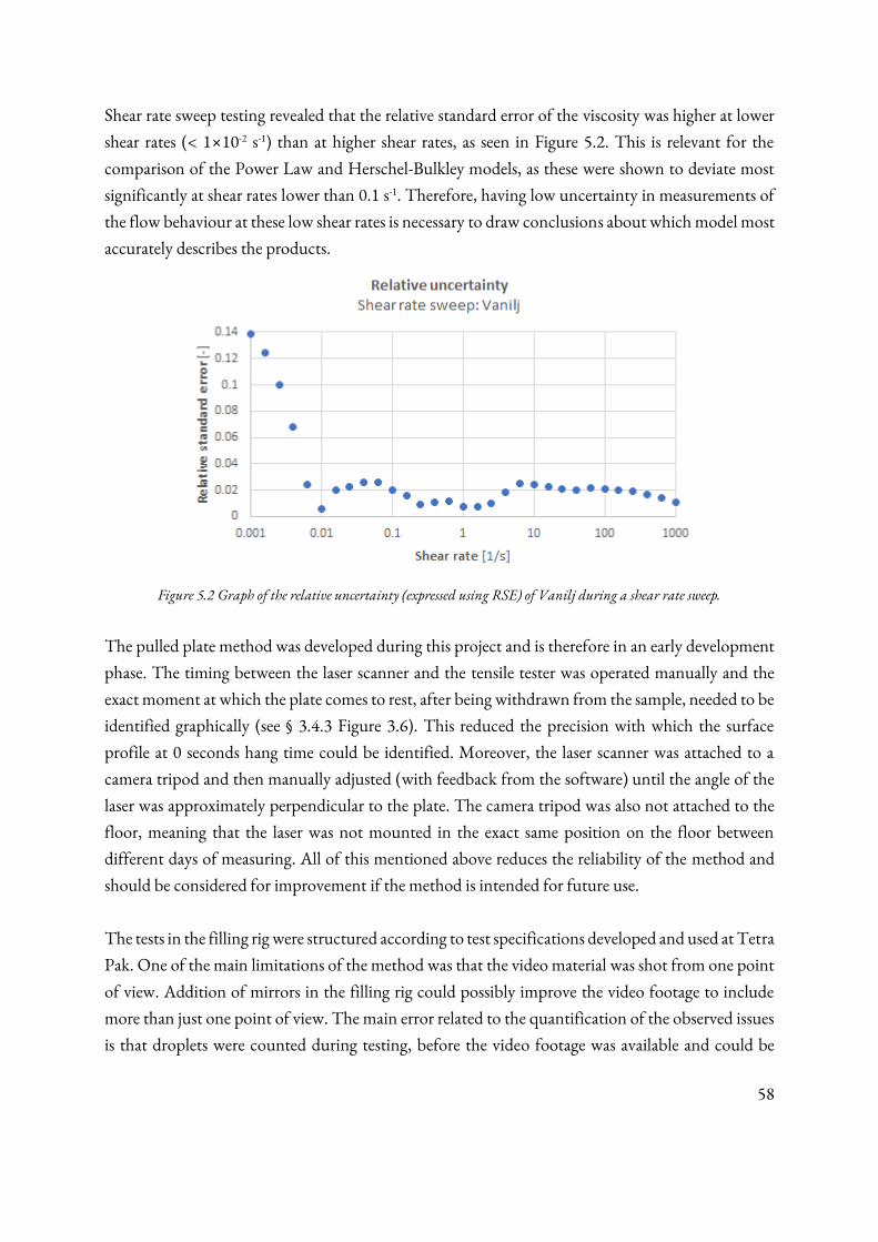
58

Shear rate sweep testing revealed that the relative standard error of the viscosity was higher at lower

shear rates (< 1×10-2 s-1) than at higher shear rates, as seen in Figure 5.2. This is relevant for the

comparison of the Power Law and Herschel-Bulkley models, as these were shown to deviate most

significantly at shear rates lower than 0.1 s-1. Therefore, having low uncertainty in measurements of

the flow behaviour at these low shear rates is necessary to draw conclusions about which model most

accurately describes the products.

Figure 5.2 Graph of the relative uncertainty (expressed using RSE) of Vanilj during a shear rate sweep.

The pulled plate method was developed during this project and is therefore in an early development

phase. The timing between the laser scanner and the tensile tester was operated manually and the

exact moment at which the plate comes to rest, after being withdrawn from the sample, needed to be

identified graphically (see § 3.4.3 Figure 3.6). This reduced the precision with which the surface

profile at 0 seconds hang time could be identified. Moreover, the laser scanner was attached to a

camera tripod and then manually adjusted (with feedback from the software) until the angle of the

laser was approximately perpendicular to the plate. The camera tripod was also not attached to the

floor, meaning that the laser was not mounted in the exact same position on the floor between

different days of measuring. All of this mentioned above reduces the reliability of the method and

should be considered for improvement if the method is intended for future use.

The tests in the filling rig were structured according to test specifications developed and used at Tetra

Pak. One of the main limitations of the method was that the video material was shot from one point

of view. Addition of mirrors in the filling rig could possibly improve the video footage to include

more than just one point of view. The main error related to the quantification of the observed issues

is that droplets were counted during testing, before the video footage was available and could be

59

studied frame by frame. This has likely contributed to some overlap in quantification of the droplets

and streaks. However, the magnitude of this overlap is unlikely to have influenced the outcomes

described in this report.

5.4.3 Error and validity

As mentioned in § 5.4.1, the precision of the Bayod yield stress determination method is highly

dependent on the number of data points taken in the shear stress sweep. As can be seen in Figure 4.3,

the true yield stress may lay in the region between the two local minima. This method is therefore

sensitive to operating conditions and may better describe the interval in which the yield stress occurs

rather than an exact yield stress value.

The shear stress controlled Tangent method was also performed by Lhamo and Nugrahini (2019),

with the results and changes to methodology shown in Appendix 8.1. The differences in the

measured yield stresses on the same samples indicate that the Tangent method is highly sensitive to

changes in methodology. It would therefore be worthwhile to investigate the impact of changes to

temperature and the use of smooth geometry on the results of this method. Additionally, the way the

tangents in the graphs are defined impacts the stress at which the intersection of the tangents occurs.

It could therefore be of interest to perform a sensitivity analysis on how the definition of the tangent

lines affects the yield stress. Further investigation may find that the Tangent method is not as valid

for yield stress determination as the results of this report suggest. However, the definition of the

tangents in this study has been consistent, and the yield stress results are comparable with each-other.

The differences measured by Lhamo and Nugrahini (2019) may be a result of any one, or a

combination of, the differences in their experimental and analysis methodologies.

The limitation of using Power Law constants in the determination of the extensional viscosity was

likely a large source of error. As mentioned in § 2.3.1 the analysis method calculates the corrected

extensional viscosity based on the deduction of the shear viscosity. As previously stated, the Herschel-

Bulkley model provided a better fit for the shear viscosity experimental data and Power Law was

shown to deviate from the Herschel-Bulkley model at low shear rates. This deviation is important as

the HCF nozzle was designed to minimise shear forces in the product flow through the nozzle. It can

be debated whether the method is successful in its assumptions and calculations, and therefore

whether the ‘true’ extensional viscosity was measured. However, the current method is sufficient for use as a behaviour indicator.

60

6 Conclusion and Recommendations This study aimed to improve the characterisation of the complex rheological behaviour of fermented

dairy products by applying a variety of measurement techniques. A review of existing experimental

techniques and rheological models was used to find suitable measurement methods. Three products

(Skånemejerier Vaniljyoghurt, Skånemejerier Naturell Lättyoghurt and Arla Långfil) were measured

with the chosen measurement methods, and a number of rheological parameters were determined

for each product. The products were also measured using two validation methods, a pulled-plate rig

and filling rig. The characterisation results were then used as inputs to CFD modelling and the pulled

plate validation results were compared with CFD results. The characterisation results were also used

for correlation with filling issues, which was able to identify potential indicators of certain

behaviours. Based on this, recommendations of experimental measurement methods and analysis

methods could be made, and thus the objectives of this study were met.

This study demonstrated that it is possible to measure the observable differences between the

products with the chosen measurement and analysis methods, using existing equipment. This was

achieved both using the rotation rheometer to determine A and b and the HCF rheometer to

determine Kε and nε. The pulled-plate rig was able to measure a difference between the yoghurt

products and Långfil. The fill rig validation methodology was also used to quantify differences

between all products in the frequencies of all behaviours were measured.

This study aimed to use a comparison between CFD modelling and experimental data to identify a

more realistic model. The method developed for measuring the profile of product along a pulled

plate was successful and proved reproducible and could be used for validating the CFD results.

However, due to complications in the CFD modelling, it was not possible to determine which

rheological model was most accurate. Instead, the results were successfully used to validate the

existence of a yield stress, especially in the Långfil sample. This implies that the Herschel-Bulkley

model better reflects reality.

The fill rig testing demonstrated that it is possible to quantify issues in automatic filling machines,

such as dripping and splashing. Based on the results from the characterisation and fill rig tests, it was

concluded that the variables A, b and nε could be measured and correlated to the filling behaviour of

the studied products. In particular, a high value for b was strongly correlated with a high frequency

of splashing and filamentation, and a low frequency of dripping. This indicates that issues during

automatic filling have the potential to be anticipated using measurable rheological properties.

61

From the investigations presented in this study, the following measurement- and analysis methods

are proposed for future characterisation of fermented dairy products:

• Linear stress ramp and Tangent analysis method for yield stress determination

• Shear rate sweep and Herschel-Bulkley curve fitting (including yield stress) for A and b

determination

• Pulled plate validation method for comparison with future CFD modelling

• Pilot scale fill rig testing for identification and quantification of issues during automatic

filling

6.1 Future work

The correlation between measurable characteristics and quantifiable filling issues was the first part

of an exploratory study, with the aim of identifying relevant rheological parameters for

characterisation, CFD modelling and behaviour prediction.The results suggest it would be

worthwhile to continue the study by determining the yield stresses and Herschel-Bulkley coefficients

of a wider selection of products to validate the correlation of A and b to filling issues. Furthermore,

systematic testing should be conducted to check whether these characteristics have an actual effect

on the filling behaviour, or whether there are other underlying causes for the correlation. This could

be achieved by mixing products with distinct properties in varying concentrations to measure the

impact of these properties, both on the measured characteristics and the filling issues.

In addition to this, several experimental variables that were not considered within the scope of this

project should be included and investigated in future studies. These include the products’ microstructure and particle size, pre-shearing, temperature dependence, pH dependence and

composition. Addition of a resting time could also potentially reduce the uncertainty of the

experimental measurements.

62

7 References

Anton Paar GmbH (2019) Basics of rheology. Available at: https://wiki.anton-paar.com/en/basics-of-rheology/ (Accessed: 21 January 2019).

Bayod, E. et al. (2007) ‘Low Shear Rheology of Concentrated Tomato Products. Effect of Particle Size and Time’, Food Biophysics. doi: 10.1007/s11483-007-9039-2.

Bayod, E. (2008) Microstructural and Rheological Properties of Concentrated Tomato Suspensions

During Processing. Lund University.

Butler, F. and McNulty, P. (1995) ‘Time dependent rheological characterisation of buttermilk at 5 °C’, Journal of Food Engineering. doi: 10.1016/0260-8774(94)00035-8.

Bylund, G. (2015) ‘Rheology’, in Dairy Processing Handbook. 2nd edn. Lund: Tetra Pak.

Cedergårdh, F. (2014) Characterization of commercial mayonnaise products Texture, Viscosity and

Droplet size. Lund University.

Chhabra, R. P. (2010) ‘Non-Newtonian fluids: An introduction’, in Symposium on Rheology of

Complex Fluids, pp. 3–34. doi: 10.1007/978-1-4419-6494-6_1.

Coussot, P. (2014) Rheophysics: Matter in All Its States, Soft and Biological Matter. doi: 10.1007/978-3-319-06148-1.

Cross, M. M. (1965) ‘Rheology of Non-Newtonian Fluids: A New Flow Equation for Pseudoplastic Systems’, Journal of Colloid Science, 20, pp. 417–437.

Fangary, Y. S., Barigou, M. and Seville, J. P. K. (1999) ‘Simulation of yoghurt flow and prediction of its end-of-process properties using rheological measurements’, Food and Bioproducts

Processing: Transactions of the Institution of of Chemical Engineers, Part C, 77, pp. 33–39. doi: 10.1205/096030899532231.

Fondén, R., Leporanta, K. and Svensson, U. (2006) ‘7 Nordic / Scandinavian Fermented Milk Products’, (2002).

Franck, A. (no date) Viscoelasticity and dynamic mechanical testing.

Gumulya, M. M., Horsley, R. R. and Pareek, V. (2014) ‘Numerical simulation of the settling behaviour of particles in thixotropic fluids’, Physics of Fluids. doi: 10.1063/1.4866320.

Håkansson, A. (2018) ‘PLS - Examples & Interpretations’. Lund: Lund University.

Javanmard, M. et al. (2018) ‘Application of the thixotropic elasto-viscoplastic model as a structure probing technique for acid milk gel suspensions’, Journal of Food Engineering. doi: 10.1016/j.jfoodeng.2017.11.031.

Jönsson, P. G. (2019) ‘Study of advanced rheology models’.

Landman, E. (2019) Viscosity Control of Solder Paste by Ultrasound Actuation. Kungliga Tekniska Högskola.

63

Larson, R. G. (1994) ‘Nonlinear Viscoelasticity’, in Macosko, C. W. (ed.) Rheology: Principles,

Measurements, and Applications. New York: Wiley VCH, pp. 135–174.

Lhamo, S. and Nugrahini, A. (2019) Understanding of product build up at packaging material

surface to address food waste. Lunds Tekniska Högskola.

Macosko, C. W. (1994) ‘Extensional Rheometry’, in Rheology : principles, measurements, and

applications. New York: Wiley-VCH , pp. 285–335.

Malvern Instruments (2012) Understanding Yield Stress Measurements. Available at: www.malvern.com/contact.

Mendes, P. R. S. and Dutra, E. S. S. (2004) ‘Viscosity function for yield-stress liquids’, Applied

Rheology, 12, pp. 296–302. Available at: https://www.researchgate.net/publication/287168717.

Mokhtari, M. (2011) ‘Thixotropic and Rheopectic Modeling of Xanthan-Borate Gel System’, in American Association of Drilling Engineers National Technical Conference and Exhibition. Houston, TX.

Moller, P. et al. (2009) ‘An attempt to categorize yield stress fluid behaviour’, Philosophical

Transactions of the Royal Society A: Mathematical, Physical and Engineering Sciences. doi: 10.1098/rsta.2009.0194.

Morea, J. O., Agnusdei, R. and Zerbino, F. (2010) ‘Comparison of methods for measuring zero shear viscosity in asphalts’, Materials and Structures, 43, pp. 499–507. doi: 10.1617/s11527-009-9506-y.

Morrison, F. A. (2001a) ‘Memory Effects: Generalized Linear Viscoelastic Fluids’, in Understanding Rheology. New York: Oxford University Press, pp. 257–304.

Morrison, F. A. (2001b) Understanding Rheology. New York: Oxford University Press.

Nyström, M. et al. (2017) ‘Hyperbolic contraction measuring systems for extensional flow’, Mechanics of Time-Dependent Materials. doi: 10.1007/s11043-017-9337-0.

Radhakrishnan, A. K. T., van Lier, J. and Clemens, F. (2018) ‘Rheology of un-sieved concentrated domestic slurry: A wide gap approach’, Water, 10(1287). doi: 10.3390/w10101287.

Rohm, H. and Jaros, D. (2010) ‘The rheology and textural properties of yoghurt’, in Texture in

Food. doi: 10.1201/9780203501276.ch13.

Stading, M. and Bohlin, L. (no date) Contraction flow measurements of extensional properties.

Steffe, J. F. (1996) Rheological Methods in Food Process Engineering. 2nd edn. East Lansing, MI: Freeman Press.

Stokes, J. R. and Frith, W. J. (2008) ‘Rheology of gelling and yielding soft matter systems’, Soft

Matter, 4(6), pp. 1133–1140. doi: 10.1039/b719677f.

Stokes, J. R. and Telford, J. H. (2004) ‘Measuring the yield behaviour of structured fluids’, Journal

of Non-Newtonian Fluid Mechanics. doi: 10.1016/j.jnnfm.2004.09.001.

64

Sunthar, P. (2010) ‘Polymer rheology’, in Rheology of Complex Fluids. New York: Springer, pp. 171–191. doi: 10.1007/978-1-4419-6494-6_8.

Tehrani, A. (2008) ‘Thixotropy in Water-Based Drilling Fluids’, Annual Transactions of the Nordic

Rheology Conference, 16.

Thermo Scientific (2015) Capillary Breakup Extensional Rheometer.

UN (2017) Goal 2 - Zero Hunger, Sustainable Development Goals. Available at: https://www.un.org/sustainabledevelopment/hunger/ (Accessed: 20 December 2018).

Zhu, J. and Mizunuma, H. (2017) ‘Shear and Extensional Flow Rheology of Mucilages Derived from Natural Foods’, Nihon Reoroji Gakkaishi. doi: 10.1678/rheology.45.91.

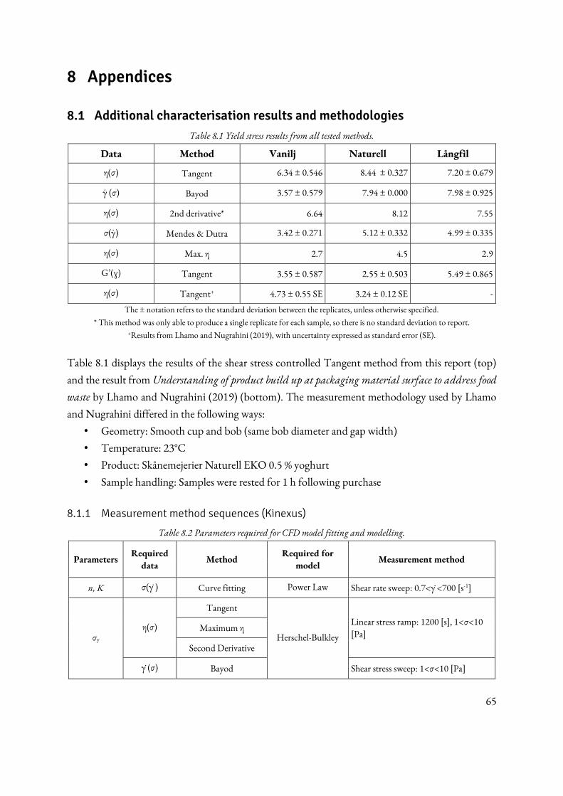
65

8 Appendices

8.1 Additional characterisation results and methodologies

Table 8.1 Yield stress results from all tested methods.

Data Method Vanilj Naturell Långfil

η(σ) Tangent 6.34 ± 0.546 8.44 ± 0.327 7.20 ± 0.679

γ ̇ (σ) Bayod 3.57 ± 0.579 7.94 ± 0.000 7.98 ± 0.925

η(σ) 2nd derivative* 6.64 8.12 7.55

σ(γ ̇) Mendes & Dutra 3.42 ± 0.271 5.12 ± 0.332 4.99 ± 0.335

η(σ) Max. η 2.7 4.5 2.9

G’(ɣ) Tangent 3.55 ± 0.587 2.55 ± 0.503 5.49 ± 0.865

η(σ) Tangent+ 4.73 ± 0.55 SE 3.24 ± 0.12 SE -

The ± notation refers to the standard deviation between the replicates, unless otherwise specified.

* This method was only able to produce a single replicate for each sample, so there is no standard deviation to report. +Results from Lhamo and Nugrahini (2019), with uncertainty expressed as standard error (SE).

Table 8.1 displays the results of the shear stress controlled Tangent method from this report (top)

and the result from Understanding of product build up at packaging material surface to address food

waste by Lhamo and Nugrahini (2019) (bottom). The measurement methodology used by Lhamo

and Nugrahini differed in the following ways:

• Geometry: Smooth cup and bob (same bob diameter and gap width)

• Temperature: 23°C

• Product: Skånemejerier Naturell EKO 0.5 % yoghurt

• Sample handling: Samples were rested for 1 h following purchase

8.1.1 Measurement method sequences (Kinexus)

Table 8.2 Parameters required for CFD model fitting and modelling.

Parameters Required

data Method

Required for

model Measurement method

n, K σ(γ ̇) Curve fitting Power Law Shear rate sweep: 0.7<γ ̇<700 [s-1]

σy η(σ)

Tangent

Herschel-Bulkley

Linear stress ramp: 1200 [s], 1<σ<10 [Pa]

Maximum η

Second Derivative

γ̇ (σ) Bayod Shear stress sweep: 1<σ<10 [Pa]

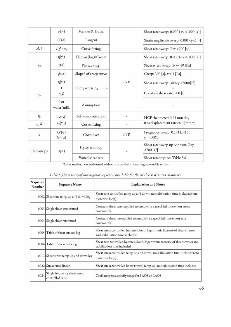
66

σ(γ ̇) Mendes & Dutra Shear rate sweep: 0.0001<γ̇ <1000 [s-1]

G’(σ) Tangent Strain amplitude sweep: 0.001<ɣ<1 [-]

A, b σ(γ ̇), σy Curve fitting Shear rate sweep: 7<γ ̇<700 [s-1]

η0

η(γ̇ ) Plateau (log)/Cross*

TVP

Shear rate sweep: 0.0001<γ̇ <1000 [s-1]

η(σ) Plateau (log) Shear stress sweep: 1<σ<10 [Pa]

ɣ(σ,t) Slope-1 of creep curve Creep: 300 [s], σ = 1 [Pa]

η∞

η(γ̇ )

+

η(t) Find η when t,γ ̇ → ∞

Shear rate sweep: 300<γ ̇<3000[s-1] +

Constant shear rate: 900 [s]

0 or

water/milk Assumption -

ηε n & K,

ηE(γ ̇E)

Software correction - HCF rheometer: 0.75 mm die, 0.6<displacement rate<6.0 [mm/s] nε, Kε Curve fitting -

θ G’(ω) G’’(ω)

Cross-over TVP Frequency sweep: 0.1<Hz<150, ɣ = 0.001

Thixotropy σ(γ ̇) Hysteresis loop

-

Shear rate sweep up & down: 7<γ ̇<700 [s-1]

Varied shear rate Shear rate step: see Table 3.8

*Cross method was performed without successfully obtaining reasonable results

Table 8.3 Summary of investigated sequences available for the Malvern Kinexus rheometer.

Sequence

Number Sequence Name Explanation and Notes

0002 Shear rate ramp up and down log Shear rate controlled ramp up and down, no stabilisation time included (one

hysteresis loop)

0003 Single shear stress timed Constant shear stress applied to sample for a specified time (shear stress controlled)

0004 Single shear rate timed Constant shear rate applied to sample for a specified time (shear rate controlled)

0005 Table of shear stresses log Shear stress controlled hysteresis loop, logarithmic increase of shear stresses and stabilisation time included

0006 Table of shear rates log Shear rate controlled hysteresis loop, logarithmic increase of shear stresses and stabilisation time included

0013 Shear stress ramp up and down log Shear stress controlled ramp up and down, no stabilisation time included (one

hysteresis loop)

0022 Stress ramp linear Shear stress controlled linear (stress) ramp up, no stabilisation time included

0024 Single frequency shear stress controlled time

Oscillatory test, specify range for SAOS or LAOS

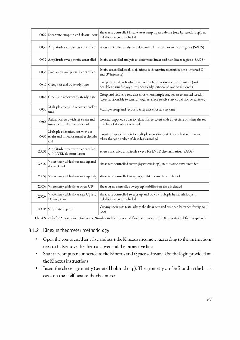
67

0027 Shear rate ramp up and down linear Shear rate controlled linear (rate) ramp up and down (one hysteresis loop), no stabilisation time included

0030 Amplitude sweep stress controlled Stress controlled analysis to determine linear and non-linear regions (SAOS)

0032 Amplitude sweep strain controlled Strain controlled analysis to determine linear and non-linear regions (SAOS)

0035 Frequency sweep strain controlled Strain controlled small oscillations to determine relaxation time (inverted G' and G'' intersect)

0040 Creep test end by steady state Creep test that ends when sample reaches an estimated steady-state (not possible to run for yoghurt since steady state could not be achieved)

0045 Creep and recovery by steady state Creep and recovery test that ends when sample reaches an estimated steady-state (not possible to run for yoghurt since steady state could not be achieved)

0053 Multiple creep and recovery end by time

Multiple creep and recovery tests that ends at a set time

0068 Relaxation test with set strain and timed or number decades end

Constant applied strain to relaxation test, test ends at set time or when the set number of decades is reached

0069 Multiple relaxation test with set strain and timed or number decades end

Constant applied strain to multiple relaxation test, test ends at set time or when the set number of decades is reached

XX01 Amplitude sweep stress controlled with LVER determination

Stress controlled amplitude sweep for LVER determination (SAOS)

XX02 Viscometry table shear rate up and down timed

Shear rate controlled sweep (hysteresis loop), stabilisation time included

XX03 Viscometry table shear rate up only Shear rate controlled sweep up, stabilisation time included

XX04 Viscometry table shear stress UP Shear stress controlled sweep up, stabilisation time included

XX05 Viscometry table shear rate Up and Down 3 times

Shear rate controlled sweeps up and down (multiple hysteresis loops), stabilisation time included

XX06 Shear rate step test Varying shear rate tests, where the shear rate and time can be varied for up to 6 stwe

The XX prefix for Measurement Sequence Number indicates a user-defined sequence, while 00 indicates a default sequence.

8.1.2 Kinexus rheometer methodology

• Open the compressed air valve and start the Kinexus rheometer according to the instructions

next to it. Remove the thermal cover and the protective bob.

• Start the computer connected to the Kinexus and rSpace software. Use the login provided on

the Kinexus instructions.

• Insert the chosen geometry (serrated bob and cup). The geometry can be found in the black

cases on the shelf next to the rheometer.

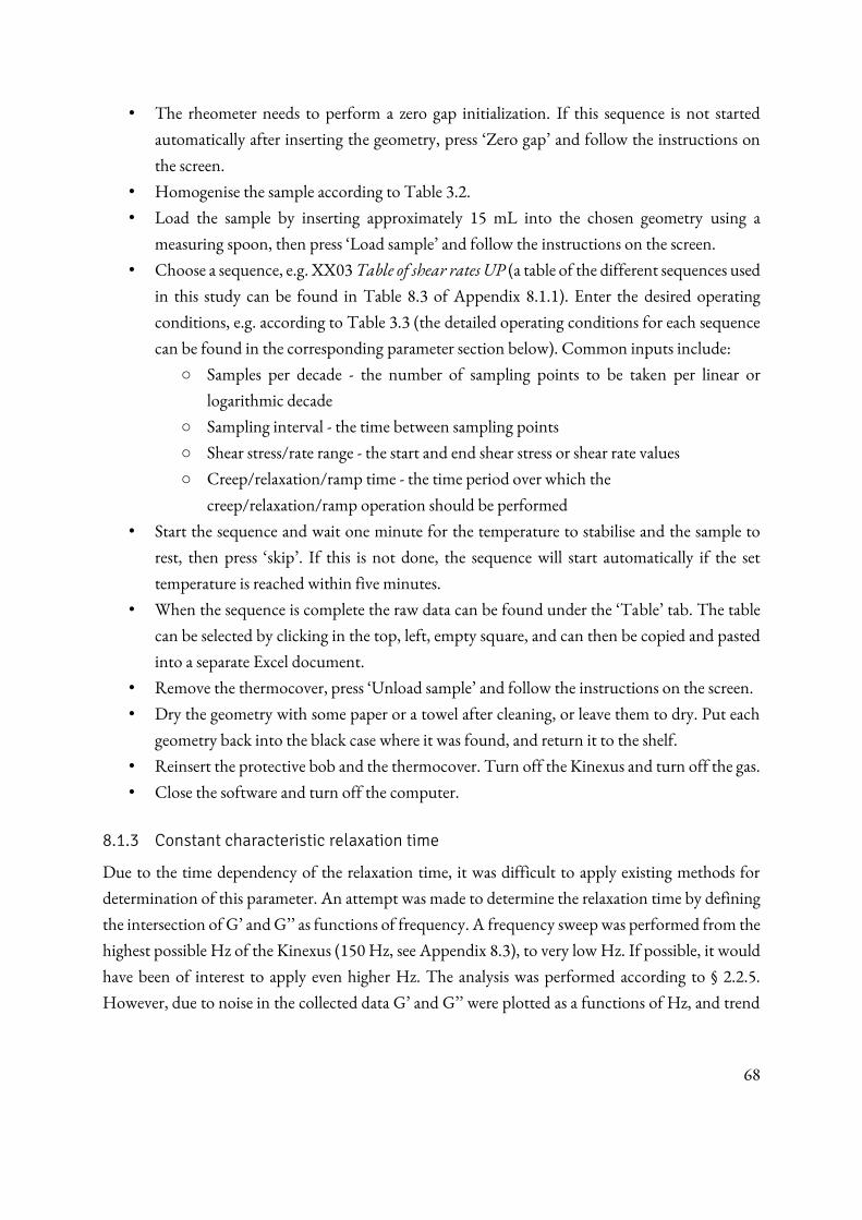
68

• The rheometer needs to perform a zero gap initialization. If this sequence is not started

automatically after inserting the geometry, press ‘Zero gap’ and follow the instructions on the screen.

• Homogenise the sample according to Table 3.2.

• Load the sample by inserting approximately 15 mL into the chosen geometry using a

measuring spoon, then press ‘Load sample’ and follow the instructions on the screen.

• Choose a sequence, e.g. XX03 Table of shear rates UP (a table of the different sequences used

in this study can be found in Table 8.3 of Appendix 8.1.1). Enter the desired operating

conditions, e.g. according to Table 3.3 (the detailed operating conditions for each sequence

can be found in the corresponding parameter section below). Common inputs include:

○ Samples per decade - the number of sampling points to be taken per linear or

logarithmic decade

○ Sampling interval - the time between sampling points

○ Shear stress/rate range - the start and end shear stress or shear rate values

○ Creep/relaxation/ramp time - the time period over which the

creep/relaxation/ramp operation should be performed

• Start the sequence and wait one minute for the temperature to stabilise and the sample to

rest, then press ‘skip’. If this is not done, the sequence will start automatically if the set

temperature is reached within five minutes.

• When the sequence is complete the raw data can be found under the ‘Table’ tab. The table can be selected by clicking in the top, left, empty square, and can then be copied and pasted

into a separate Excel document.

• Remove the thermocover, press ‘Unload sample’ and follow the instructions on the screen.

• Dry the geometry with some paper or a towel after cleaning, or leave them to dry. Put each

geometry back into the black case where it was found, and return it to the shelf.

• Reinsert the protective bob and the thermocover. Turn off the Kinexus and turn off the gas.

• Close the software and turn off the computer.

8.1.3 Constant characteristic relaxation time

Due to the time dependency of the relaxation time, it was difficult to apply existing methods for

determination of this parameter. An attempt was made to determine the relaxation time by defining

the intersection of G’ and G’’ as functions of frequency. A frequency sweep was performed from the

highest possible Hz of the Kinexus (150 Hz, see Appendix 8.3), to very low Hz. If possible, it would

have been of interest to apply even higher Hz. The analysis was performed according to § 2.2.5.

However, due to noise in the collected data G’ and G’’ were plotted as a functions of Hz, and trend

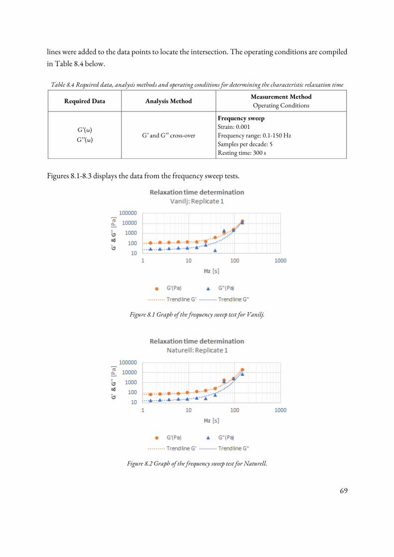
69

lines were added to the data points to locate the intersection. The operating conditions are compiled

in Table 8.4 below.

Table 8.4 Required data, analysis methods and operating conditions for determining the characteristic relaxation time



G’(ω)

G’’(ω) G’ and G’’ cross-over

Frequency sweep

Strain: 0.001 Frequency range: 0.1-150 Hz Samples per decade: 5 Resting time: 300 s

Figures 8.1-8.3 displays the data from the frequency sweep tests.

Figure 8.1 Graph of the frequency sweep test for Vanilj.

Figure 8.2 Graph of the frequency sweep test for Naturell.

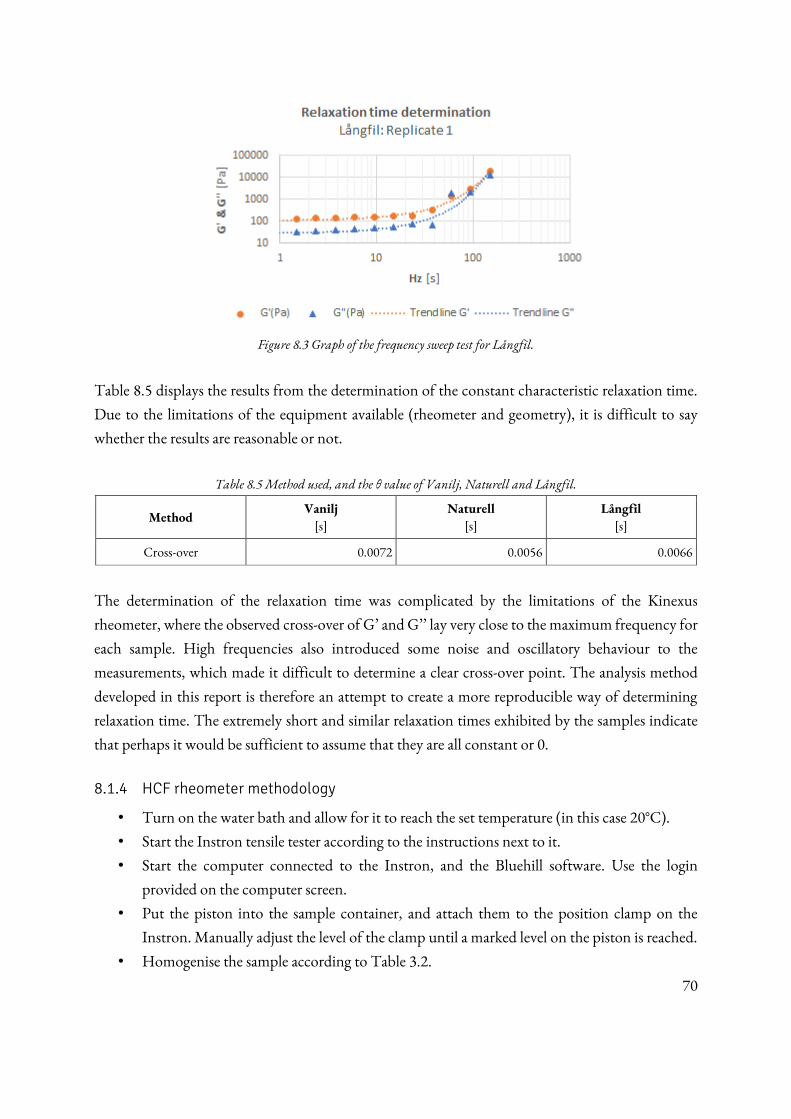
70

Figure 8.3 Graph of the frequency sweep test for Långfil.

Table 8.5 displays the results from the determination of the constant characteristic relaxation time.

Due to the limitations of the equipment available (rheometer and geometry), it is difficult to say

whether the results are reasonable or not.

Table 8.5 Method used, and the θ value of Vanilj, Naturell and Långfil.

Method Vanilj

[s] Naturell

[s] Långfil

[s]

Cross-over 0.0072 0.0056 0.0066

The determination of the relaxation time was complicated by the limitations of the Kinexus

rheometer, where the observed cross-over of G’ and G’’ lay very close to the maximum frequency for each sample. High frequencies also introduced some noise and oscillatory behaviour to the

measurements, which made it difficult to determine a clear cross-over point. The analysis method

developed in this report is therefore an attempt to create a more reproducible way of determining

relaxation time. The extremely short and similar relaxation times exhibited by the samples indicate

that perhaps it would be sufficient to assume that they are all constant or 0.

8.1.4 HCF rheometer methodology

• Turn on the water bath and allow for it to reach the set temperature (in this case 20°C).

• Start the Instron tensile tester according to the instructions next to it.

• Start the computer connected to the Instron, and the Bluehill software. Use the login

provided on the computer screen.

• Put the piston into the sample container, and attach them to the position clamp on the

Instron. Manually adjust the level of the clamp until a marked level on the piston is reached.


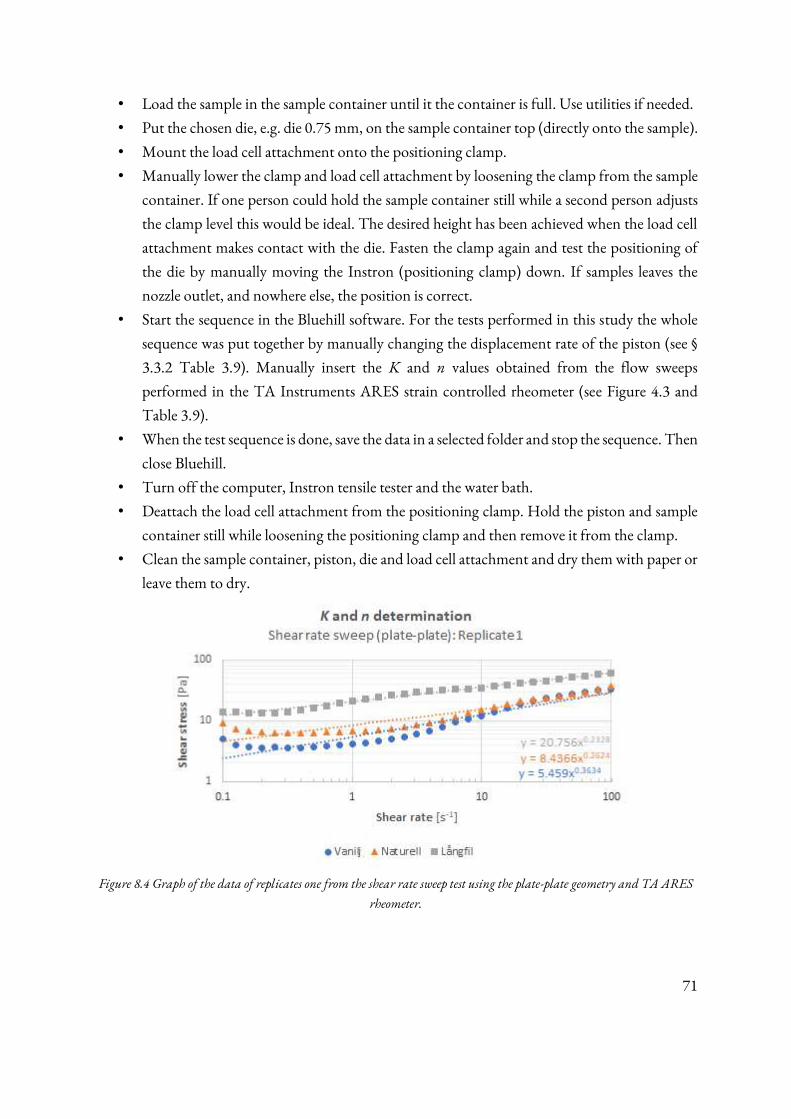
71

• Load the sample in the sample container until it the container is full. Use utilities if needed.

• Put the chosen die, e.g. die 0.75 mm, on the sample container top (directly onto the sample).

• Mount the load cell attachment onto the positioning clamp.

• Manually lower the clamp and load cell attachment by loosening the clamp from the sample

container. If one person could hold the sample container still while a second person adjusts

the clamp level this would be ideal. The desired height has been achieved when the load cell

attachment makes contact with the die. Fasten the clamp again and test the positioning of

the die by manually moving the Instron (positioning clamp) down. If samples leaves the

nozzle outlet, and nowhere else, the position is correct.

• Start the sequence in the Bluehill software. For the tests performed in this study the whole

sequence was put together by manually changing the displacement rate of the piston (see §

3.3.2 Table 3.9). Manually insert the K and n values obtained from the flow sweeps

performed in the TA Instruments ARES strain controlled rheometer (see Figure 4.3 and

Table 3.9).

• When the test sequence is done, save the data in a selected folder and stop the sequence. Then

close Bluehill.

• Turn off the computer, Instron tensile tester and the water bath.

• Deattach the load cell attachment from the positioning clamp. Hold the piston and sample

container still while loosening the positioning clamp and then remove it from the clamp.

• Clean the sample container, piston, die and load cell attachment and dry them with paper or

leave them to dry.

Figure 8.4 Graph of the data of replicates one from the shear rate sweep test using the plate-plate geometry and TA ARES

rheometer.

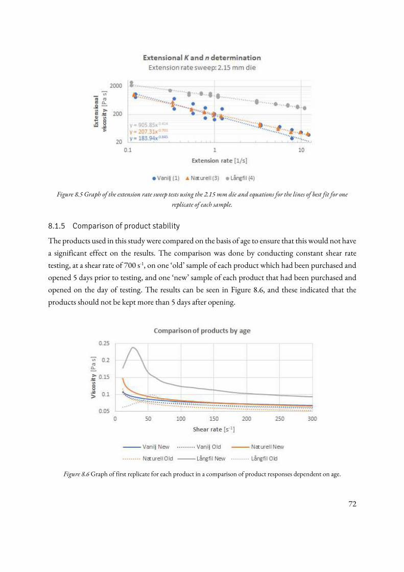
72

Figure 8.5 Graph of the extension rate sweep tests using the 2.15 mm die and equations for the lines of best fit for one

replicate of each sample.

8.1.5 Comparison of product stability

The products used in this study were compared on the basis of age to ensure that this would not have

a significant effect on the results. The comparison was done by conducting constant shear rate

testing, at a shear rate of 700 s-1, on one ‘old’ sample of each product which had been purchased and opened 5 days prior to testing, and one ‘new’ sample of each product that had been purchased and

opened on the day of testing. The results can be seen in Figure 8.6, and these indicated that the

products should not be kept more than 5 days after opening.

Figure 8.6 Graph of first replicate for each product in a comparison of product responses dependent on age.

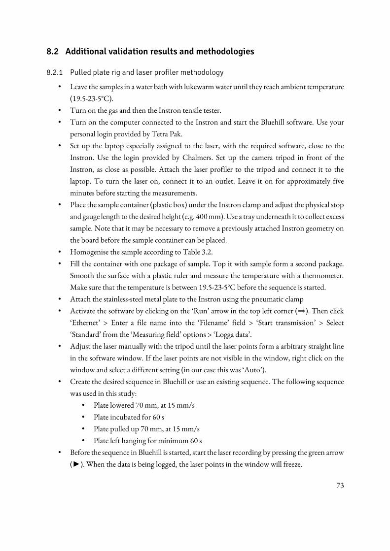
73

8.2 Additional validation results and methodologies

8.2.1 Pulled plate rig and laser profiler methodology

• Leave the samples in a water bath with lukewarm water until they reach ambient temperature

(19.5-23-5°C).

• Turn on the gas and then the Instron tensile tester.

• Turn on the computer connected to the Instron and start the Bluehill software. Use your

personal login provided by Tetra Pak.

• Set up the laptop especially assigned to the laser, with the required software, close to the

Instron. Use the login provided by Chalmers. Set up the camera tripod in front of the

Instron, as close as possible. Attach the laser profiler to the tripod and connect it to the

laptop. To turn the laser on, connect it to an outlet. Leave it on for approximately five

minutes before starting the measurements.

• Place the sample container (plastic box) under the Instron clamp and adjust the physical stop

and gauge length to the desired height (e.g. 400 mm). Use a tray underneath it to collect excess

sample. Note that it may be necessary to remove a previously attached Instron geometry on

the board before the sample container can be placed.


• Fill the container with one package of sample. Top it with sample form a second package.

Smooth the surface with a plastic ruler and measure the temperature with a thermometer.

Make sure that the temperature is between 19.5-23-5°C before the sequence is started.

• Attach the stainless-steel metal plate to the Instron using the pneumatic clamp

• Activate the software by clicking on the ‘Run’ arrow in the top left corner (⇒). Then click ‘Ethernet’ > Enter a file name into the ‘Filename’ field > ‘Start transmission’ > Select ‘Standard’ from the ‘Measuring field’ options > ‘Logga data’.

• Adjust the laser manually with the tripod until the laser points form a arbitrary straight line

in the software window. If the laser points are not visible in the window, right click on the

window and select a different setting (in our case this was ‘Auto’). • Create the desired sequence in Bluehill or use an existing sequence. The following sequence

was used in this study:

• Plate lowered 70 mm, at 15 mm/s

• Plate incubated for 60 s

• Plate pulled up 70 mm, at 15 mm/s

• Plate left hanging for minimum 60 s

• Before the sequence in Bluehill is started, start the laser recording by pressing the green arrow

(►). When the data is being logged, the laser points in the window will freeze.

74

• Press ‘Return’ > ‘Reset gauge’ > ‘Balance load’. Start the Bluehill sequence. Run the sequence five times. Adjust the sample container’s position between each cycle so that the plate is inserted in a different place in the yoghurt each time.

• When the sequence is over, save the data and then stop the sequence.

• Stop the laser measurement by clicking on ‘Logga Data’. The data is saved to a folder on the

computer. It is possible to change this folder in the software. Press ‘Stop VI’ to stop the sequence.

• When the testing is done, close the softwares on each computer and turn them both off.

Disconnect the laser from the laptop and remove it from the tripod. Put them away on their

assigned places.

• Remove the metal plate from the Instron pneumatic clamp. Clean the plate, sample

container, tray and ruler. Dry with paper or leave them to dry.

8.2.2 Stand-alone fill rig methodology

• Leave the samples in room temperature overnight, to allow for them to reach ambient

temperature.

• Fill the holding tank manually by emptying the packages into it until a marked tank level is

reached. Note that the samples were not homogenised according to Table 3.2 before the

holding tank was filled with the samples.

○ Långfil was homogenised by inverting each package 10 times

○ Vanilj and Naturell were homogenised by inverting each package 2 times

• Measure the temperature at the bottom of the holding tank with a thermometer. The

temperature is to be noted on the test record.

• The filling rig is monitored and run by the responsible Tetra Pak employees, with the settings

defined in Table 3.9. One test sequence was compiled of 12 cycles in the following order:

MOD (×3), STD (×3), MOD (×3) and STD (×3). Each cycle consisted of ten filling shots,

for a total of 120.

• The filling was filmed, by a Tetra Pak employee, with a digital camera (iPhone) and pictures

were taken after 10 filling shots.

• The filling nozzle, transparent package and board were cleaned after 10 filling shots and after

the pictures had been taken.

• When the testing was done, the filling rig was emptied by the responsible Tetra Pak employee

and cleaned by CIP.

• The video material was then analysed frame by frame so that issues and events could be

grouped together, defined and correlated to the results from the characterisation phase.

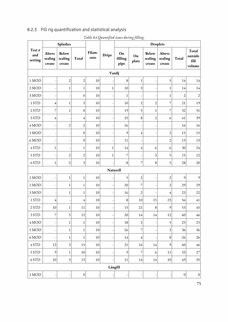
75

8.2.3 Fill rig quantification and statistical analysis

Table 8.6 Quantified issues during filling.

Test #

and

setting

Splashes

Filam-

ents Drips

Droplets

Above

sealing

crease

Below

sealing

crease

Total On

filling

pipe

On

plate

Below

sealing

crease

Above

sealing

crease

Total

Total

outside

fill

volume

Vanilj

1 MOD - 2 2 10 - 8 1 - 5 14 14

2 MOD - 1 1 10 1 10 3 - 1 14 14

3 MOD - - 0 10 - 1 - - 1 2 2

1 STD 4 1 5 10 - 10 2 2 7 21 19

2 STD 7 1 8 10 - 19 5 1 7 32 31

3 STD 4 - 4 10 - 25 8 2 6 41 39

4 MOD - 2 2 10 - 16 - - - 16 16

5 MOD - - 0 10 - 9 4 - 2 15 15

6 MOD - - 0 10 - 11 - - 2 13 13

4 STD 1 - 1 10 1 14 4 6 6 30 24

5 STD - 2 2 10 1 7 - 3 5 15 12

6 STD 1 2 3 10 - 8 7 8 5 28 20

Naturell

1 MOD - 1 1 10 - 5 2 - 2 9 9

2 MOD - 1 1 10 - 20 7 - 2 29 29

3 MOD - 1 1 10 - 16 2 - 4 23 22

1 STD 4 - 4 10 - 8 10 15 23 56 41

2 STD 10 1 11 10 - 15 21 8 9 53 45

3 STD 7 5 12 10 - 20 14 14 12 60 46

4 MOD - 1 1 10 - 18 2 - 5 25 25

5 MOD - 1 1 10 - 26 7 - 3 36 36

6 MOD - 1 1 10 - 14 4 - 8 26 26

4 STD 12 3 15 10 - 21 16 14 9 60 46

5 STD 9 1 10 10 - 9 7 6 11 33 27

6 STD 10 3 13 10 - 11 14 14 10 49 35

Långfil

1 MOD - - 0 - - - - - - 0 0

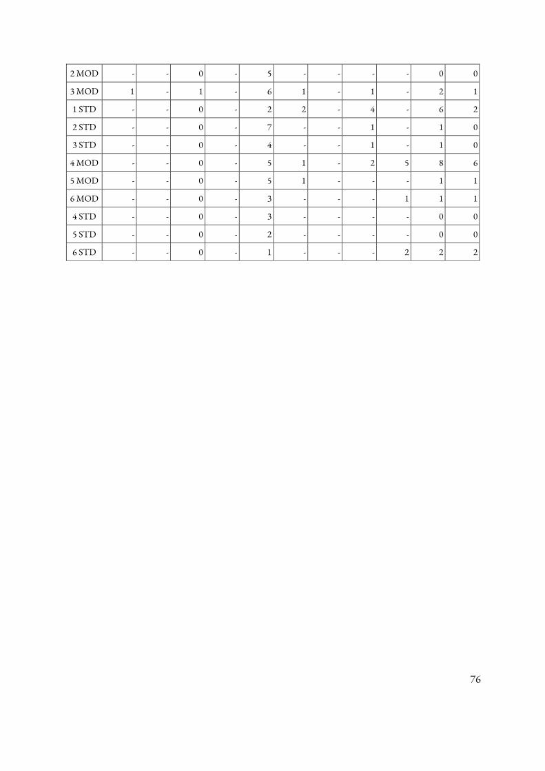
76

2 MOD - - 0 - 5 - - - - 0 0

3 MOD 1 - 1 - 6 1 - 1 - 2 1

1 STD - - 0 - 2 2 - 4 - 6 2

2 STD - - 0 - 7 - - 1 - 1 0

3 STD - - 0 - 4 - - 1 - 1 0

4 MOD - - 0 - 5 1 - 2 5 8 6

5 MOD - - 0 - 5 1 - - - 1 1

6 MOD - - 0 - 3 - - - 1 1 1

4 STD - - 0 - 3 - - - - 0 0

5 STD - - 0 - 2 - - - - 0 0

6 STD - - 0 - 1 - - - 2 2 2

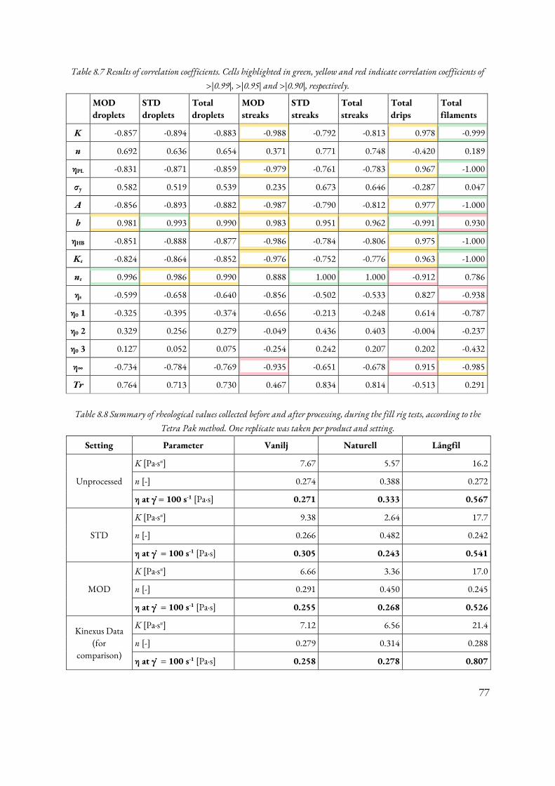
77

Table 8.7 Results of correlation coefficients. Cells highlighted in green, yellow and red indicate correlation coefficients of

>|0.99|, >|0.95| and >|0.90|, respectively.

MOD

droplets

STD

droplets

Total

droplets

MOD

streaks

STD

streaks

Total

streaks

Total

drips

Total

filaments

K -0.857 -0.894 -0.883 -0.988 -0.792 -0.813 0.978 -0.999

n 0.692 0.636 0.654 0.371 0.771 0.748 -0.420 0.189

ηPL -0.831 -0.871 -0.859 -0.979 -0.761 -0.783 0.967 -1.000

σy 0.582 0.519 0.539 0.235 0.673 0.646 -0.287 0.047

A -0.856 -0.893 -0.882 -0.987 -0.790 -0.812 0.977 -1.000

b 0.981 0.993 0.990 0.983 0.951 0.962 -0.991 0.930

ηHB -0.851 -0.888 -0.877 -0.986 -0.784 -0.806 0.975 -1.000

Kε -0.824 -0.864 -0.852 -0.976 -0.752 -0.776 0.963 -1.000

nε 0.996 0.986 0.990 0.888 1.000 1.000 -0.912 0.786

ηε -0.599 -0.658 -0.640 -0.856 -0.502 -0.533 0.827 -0.938

η0 1 -0.325 -0.395 -0.374 -0.656 -0.213 -0.248 0.614 -0.787

η0 2 0.329 0.256 0.279 -0.049 0.436 0.403 -0.004 -0.237

η0 3 0.127 0.052 0.075 -0.254 0.242 0.207 0.202 -0.432

η∞ -0.734 -0.784 -0.769 -0.935 -0.651 -0.678 0.915 -0.985

Tr 0.764 0.713 0.730 0.467 0.834 0.814 -0.513 0.291

Table 8.8 Summary of rheological values collected before and after processing, during the fill rig tests, according to the

Tetra Pak method. One replicate was taken per product and setting.

Setting Parameter Vanilj Naturell Långfil

Unprocessed

K [Pa∙sn] 7.67 5.57 16.2

n [-] 0.274 0.388 0.272

η at γ̇ = 100 s-1 [Pa∙s] 0.271 0.333 0.567

STD

K [Pa∙sn] 9.38 2.64 17.7

n [-] 0.266 0.482 0.242

η at γ̇ = 100 s-1 [Pa∙s] 0.305 0.243 0.541

MOD

K [Pa∙sn] 6.66 3.36 17.0

n [-] 0.291 0.450 0.245

η at γ̇ = 100 s-1 [Pa∙s] 0.255 0.268 0.526

Kinexus Data (for

comparison)

K [Pa∙sn] 7.12 6.56 21.4

n [-] 0.279 0.314 0.288

η at γ̇ = 100 s-1 [Pa∙s] 0.258 0.278 0.807

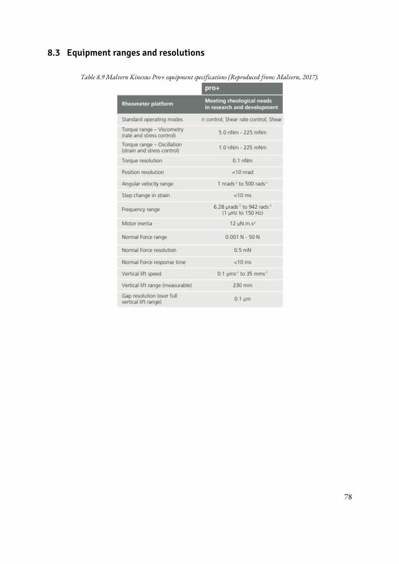
78

8.3 Equipment ranges and resolutions

Table 8.9 Malvern Kinexus Pro+ equipment specifications (Reproduced from: Malvern, 2017).

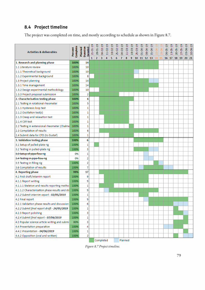
79

8.4 Project timeline

The project was completed on time, and mostly according to schedule as shown in Figure 8.7.

Figure 8.7 Project timeline.

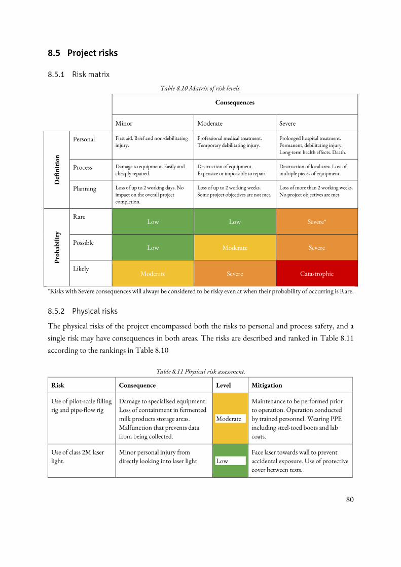
80

8.5 Project risks

8.5.1 Risk matrix

Table 8.10 Matrix of risk levels.

Consequences

Minor Moderate Severe

Def

init

ion

Personal First aid. Brief and non-debilitating injury.

Professional medical treatment. Temporary debilitating injury.

Prolonged hospital treatment. Permanent, debilitating injury. Long-term health effects. Death.

Process Damage to equipment. Easily and cheaply repaired.

Destruction of equipment. Expensive or impossible to repair.

Destruction of local area. Loss of multiple pieces of equipment.

Planning Loss of up to 2 working days. No impact on the overall project completion.

Loss of up to 2 working weeks. Some project objectives are not met.

Loss of more than 2 working weeks. No project objectives are met.

Pro

bab

ilit

y

Rare Low Low Severe*

Possible Low Moderate Severe

Likely Moderate Severe Catastrophic

*Risks with Severe consequences will always be considered to be risky even at when their probability of occurring is Rare.

8.5.2 Physical risks

The physical risks of the project encompassed both the risks to personal and process safety, and a

single risk may have consequences in both areas. The risks are described and ranked in Table 8.11

according to the rankings in Table 8.10

Table 8.11 Physical risk assessment.

Risk Consequence Level Mitigation

Use of pilot-scale filling rig and pipe-flow rig

Damage to specialised equipment. Loss of containment in fermented milk products storage areas. Malfunction that prevents data from being collected.

Moderate

Maintenance to be performed prior to operation. Operation conducted by trained personnel. Wearing PPE including steel-toed boots and lab coats.

Use of class 2M laser light.

Minor personal injury from directly looking into laser light Low

Face laser towards wall to prevent accidental exposure. Use of protective cover between tests.

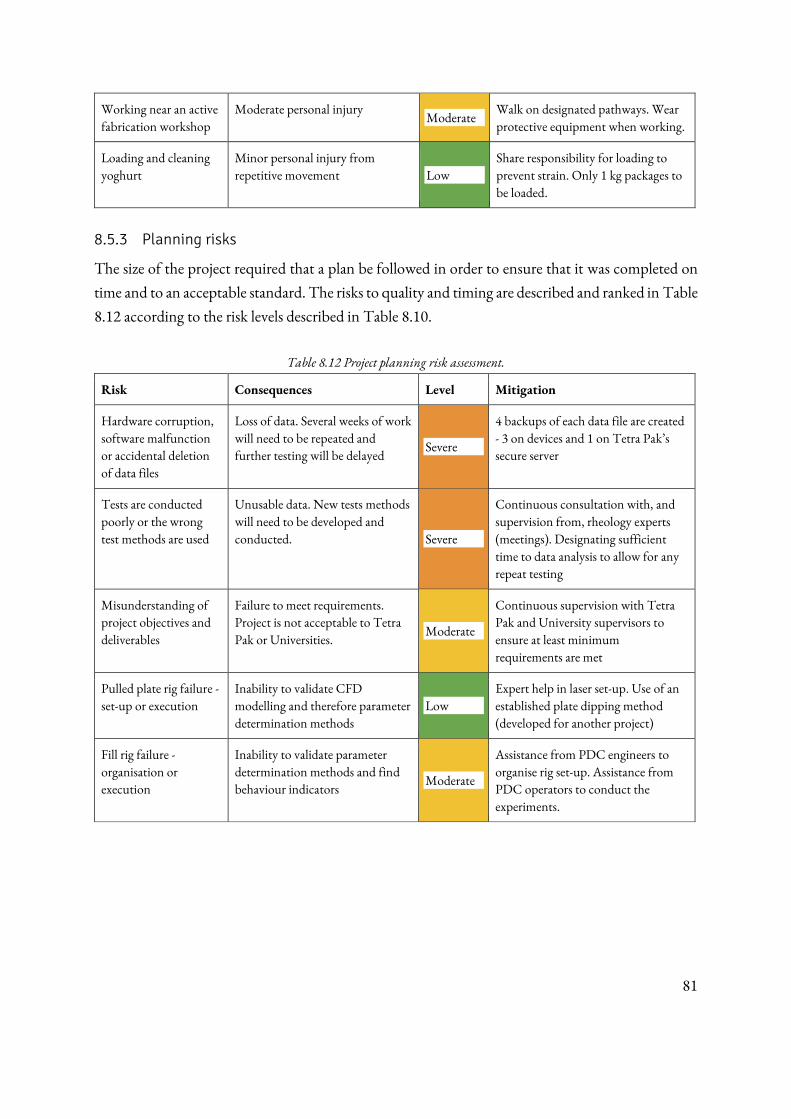
81

Working near an active fabrication workshop

Moderate personal injury Moderate

Walk on designated pathways. Wear protective equipment when working.

Loading and cleaning yoghurt

Minor personal injury from repetitive movement Low

Share responsibility for loading to prevent strain. Only 1 kg packages to be loaded.

8.5.3 Planning risks

The size of the project required that a plan be followed in order to ensure that it was completed on

time and to an acceptable standard. The risks to quality and timing are described and ranked in Table

8.12 according to the risk levels described in Table 8.10.

Table 8.12 Project planning risk assessment.

Risk Consequences Level Mitigation

Hardware corruption, software malfunction or accidental deletion of data files

Loss of data. Several weeks of work will need to be repeated and further testing will be delayed

Severe

4 backups of each data file are created - 3 on devices and 1 on Tetra Pak’s secure server

Tests are conducted poorly or the wrong test methods are used

Unusable data. New tests methods will need to be developed and conducted. Severe

Continuous consultation with, and supervision from, rheology experts (meetings). Designating sufficient time to data analysis to allow for any repeat testing

Misunderstanding of project objectives and deliverables

Failure to meet requirements. Project is not acceptable to Tetra Pak or Universities.

Moderate

Continuous supervision with Tetra Pak and University supervisors to ensure at least minimum requirements are met

Pulled plate rig failure - set-up or execution

Inability to validate CFD modelling and therefore parameter determination methods

Low Expert help in laser set-up. Use of an established plate dipping method (developed for another project)

Fill rig failure - organisation or execution

Inability to validate parameter determination methods and find behaviour indicators

Moderate

Assistance from PDC engineers to organise rig set-up. Assistance from PDC operators to conduct the experiments.

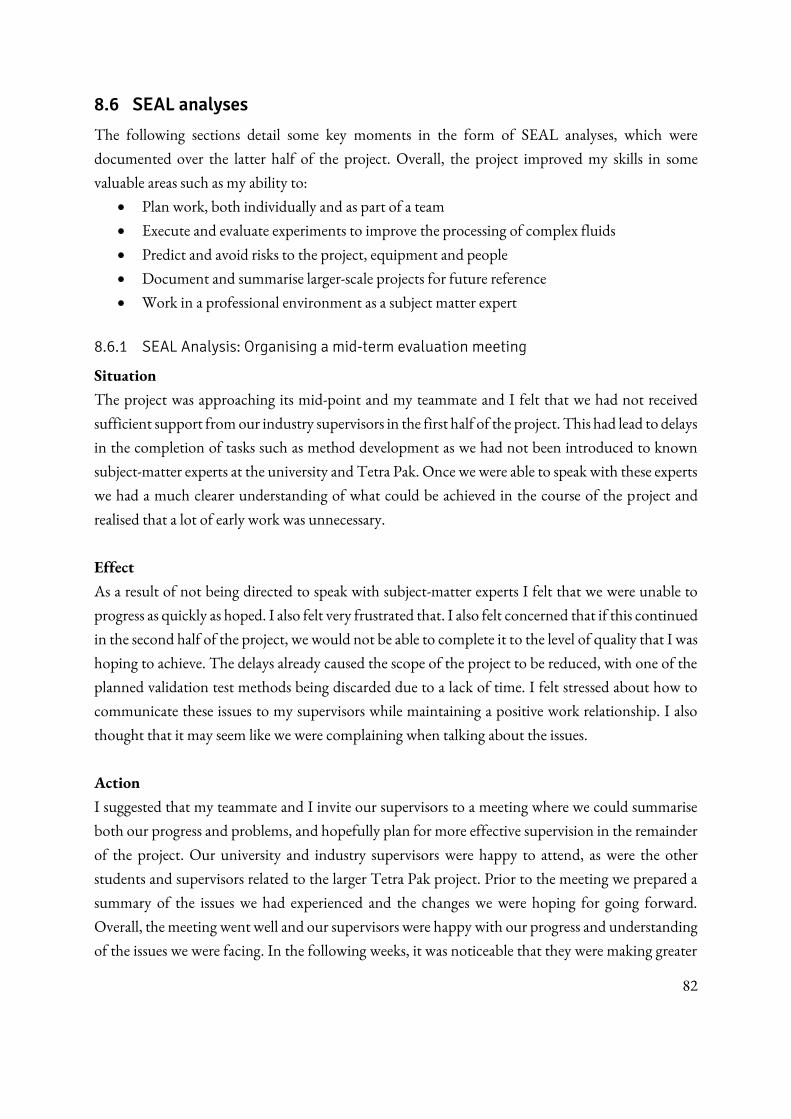
82

8.6 SEAL analyses

The following sections detail some key moments in the form of SEAL analyses, which were

documented over the latter half of the project. Overall, the project improved my skills in some

valuable areas such as my ability to:

• Plan work, both individually and as part of a team

• Execute and evaluate experiments to improve the processing of complex fluids

• Predict and avoid risks to the project, equipment and people

• Document and summarise larger-scale projects for future reference

• Work in a professional environment as a subject matter expert

8.6.1 SEAL Analysis: Organising a mid-term evaluation meeting

Situation

The project was approaching its mid-point and my teammate and I felt that we had not received

sufficient support from our industry supervisors in the first half of the project. This had lead to delays

in the completion of tasks such as method development as we had not been introduced to known

subject-matter experts at the university and Tetra Pak. Once we were able to speak with these experts

we had a much clearer understanding of what could be achieved in the course of the project and

realised that a lot of early work was unnecessary.

Effect

As a result of not being directed to speak with subject-matter experts I felt that we were unable to

progress as quickly as hoped. I also felt very frustrated that. I also felt concerned that if this continued

in the second half of the project, we would not be able to complete it to the level of quality that I was

hoping to achieve. The delays already caused the scope of the project to be reduced, with one of the

planned validation test methods being discarded due to a lack of time. I felt stressed about how to

communicate these issues to my supervisors while maintaining a positive work relationship. I also

thought that it may seem like we were complaining when talking about the issues.

Action

I suggested that my teammate and I invite our supervisors to a meeting where we could summarise

both our progress and problems, and hopefully plan for more effective supervision in the remainder

of the project. Our university and industry supervisors were happy to attend, as were the other

students and supervisors related to the larger Tetra Pak project. Prior to the meeting we prepared a

summary of the issues we had experienced and the changes we were hoping for going forward.

Overall, the meeting went well and our supervisors were happy with our progress and understanding

of the issues we were facing. In the following weeks, it was noticeable that they were making greater

83

effort to give us guidance and take a more active role in supervision, including organising meetings

to help us prioritise information in the report and plan future testing.

Learning

This event reinforced my previous opinion that it is best to communicate issues in a direct but

thoughtful manner. I think that the method we used, where we cited specific examples, outcomes

and desired changes in a calm and formal way, helped get our point across without making any

supervisors feel like they were being blamed or vilified. The meeting setting also gave them an

opportunity to give me feedback on how they perceived my progress and how I could better ask for

help in the future. Overall, it was a positive experience even though I felt very stressed and uncertain

at the start.

8.6.2 SEAL Analysis: Conducting and completing pilot-scale testing

Situation

I conducted one week of pilot-scale testing where a stand-alone fill rig was used to simulate filling the

different samples. This involved instructing and coordinating with engineering supervisors, technical

staff, and external suppliers. Myself and another student were accountable for the proper

organisation and execution of the testing, with the help of other engineering staff when we requested

it. At the end of the testing, I needed to report on whether it was complete or some testing needed to

be re-run as the testing time was limited

Effect

The pilot-scale testing was very important as it would be used for both validating our hypotheses

about the product behaviour and correlating lab-scale measurements for use as indicators. Therefore,

I felt pressure to ensure that the results we obtained from the testing would be useful and yield good

quality data. This type of test had been run before so the method development aspect was smaller,

but I knew that I would need to spend time considering as many factors as possible to make sure that

the testing time was used. I also had to plan my time in advance to ensure that there would be enough

time during testing to review the data so that any necessary adjustments could be made. This meant

that I needed to be very organised when reviewing the data that had been collected, and make a clear

decision on whether the rig was still needed.

Action

There were three test-readiness meetings conducted prior to the week of testing, and during these

meetings I aimed to clearly define the scope and purpose of the testing. I also gathered feedback from

the experts who were attending these meetings, to make sure that the scope of the test was reasonable

84

and that it had a good chance of producing results that could be used in the way I had planned. My

thesis partner and I organise the samples well in advance of the testing and so that they would have

time to be delivered and be conditioned prior to testing. We developed a log sheet so that as much

data as possible could be collected during the tests, with the remaining data to be collected by

reviewing the film footage. This allowed me to see that the expected differences between samples

were being shown in the tests, so I could definitively say that the test had been successful. Later review

of the film footage confirmed that I was correct, which supports this method of continuously

collecting and reviewing results.

Learning

Conducting and completing pilot-scale testing was the biggest responsibility I have had in this project

to date but I also feel that it gave me the greatest opportunity to demonstrate my engineering skills in

planning, co-ordinating, and justifying the testing at this scale. My method of starting the planning

relatively early and continuously reviewing the results meant that the tests took exactly the amount

of time I planned for while still achieving the aim. This has reinforced previous lessons in organisation

and sufficient communication, so I will continue to use these strategies of frequently meeting,

discussing, and planning prior to large tests like this in the future.

8.6.3 SEAL Analysis: Thesis defense at Lund University

Situation

The presentation of my project was done in conjunction with two other students from the university

who were working jointly with me and on a parallel project. This was decided by Tetra Pak and our

supervisors as the results of the two projects were intended to support one-another. Unfortunately,

the results of the modelling that was done in the other project were not helpful for us drawing

conclusions. Also, with three students presenting, it was expected that we would present for 50

minutes and have 10-20 minutes for questions.

Effect

Presenting with two other students meant that I would need to both present how my project and

results were important in isolation and with relation to the parallel mechanical engineering project.

There were no strict guidelines on how to present, so it required us to decide on a format that we

thought would best present both projects individually and as a part of a greater whole. We would

also be presenting for much longer than usual, meaning that our presentation would need to move

quickly to keep the audience’s attention.

85

With the lack of helpful results from the CFD project, there was a greater focus on our correlation

and characterization project. Around 40 minutes of the presentation were dedicated to this.

Action

Initially, we structured the presentation based on our reports so that we had a sense of what

information we had to work with. I then suggested that we group our slides so that the parts of our

reports that were dependent on each-other were together and followed in a logical sequence. This

helped to combine the information and immediately cut down on the number of slides as there was

a lot of repetition. We then decided which parts we each considered to be essential to our own work

and went through all ‘non-essential’ information to either summarise it briefly or remove it from the presentation. This was the most difficult part, as all parts had some relevance to the result, but

eventually we were able to trim the presentation down sufficiently.

Then, to make sure that we moved quickly, both due to time constraints and to keep the presentation

within the time limit, we decided to individually write scripts for our slides. We then practiced based

on these scripts and continued to trim the presentation down until we were within the time limit.

Learning

Having to condense such a huge project into a 50-minute presentation really helped to reveal what

the essential information and results were. It also impressed the importance of practicing

presentations. Because of this, we were able to give a very information dense presentation and

received feedback that it went quickly and didn’t drag. I also thought that my strategy of including all the information at first and then reducing it as a group was effective. I think it would have been

very difficult to decide what information to include as a group if we were starting from a blank

presentation.

I also learned that it can be helpful to group related projects when presenting them. If we had

presented individually then there would have been a lot of repetition of some shared key points and

a lot of other information would have been left out so that each person could cover these key points.

Instead, we were able to include much more information from each project than expected!

HE UNIVERSITY OF QUEENSLAND

Documents

Transcript of HE UNIVERSITY OF QUEENSLAND