He Loves Me, He Loves Me Not A Forecast of U.S. Jewelry Sales Alex Gates Ling-Ching Hsu Shih-Hao Lee...
28
He Loves Me, He Loves Me Not A Forecast of U.S. Jewelry Sales Alex Gates Ling-Ching Hsu Shih-Hao Lee Hui Liang Mateusz Tracz Grant Volk June 1, 2010
-
date post
22-Dec-2015 -
Category
Documents
-
view
215 -
download
0
Transcript of He Loves Me, He Loves Me Not A Forecast of U.S. Jewelry Sales Alex Gates Ling-Ching Hsu Shih-Hao Lee...

He Loves Me,He Loves Me Not
A Forecast of U.S. Jewelry SalesAlex Gates
Ling-Ching Hsu
Shih-Hao Lee
Hui Liang
Mateusz Tracz
Grant Volk
June 1, 2010

Purpose
Examine trends in jewelry sales in the United States
Create a model capable of forecasting future U.S. jewelry sales
Forecast U.S. jewelry sales for one year

Data
Data obtained from U.S. Census Bureau website (http://www.census.gov/retail)
Data is monthly U.S. Jewelry Sales from January, 1992 through March, 2010

Jewelry Sales Data (JSALES)
0
2000
4000
6000
8000
92 94 96 98 00 02 04 06 08 10
JSALES
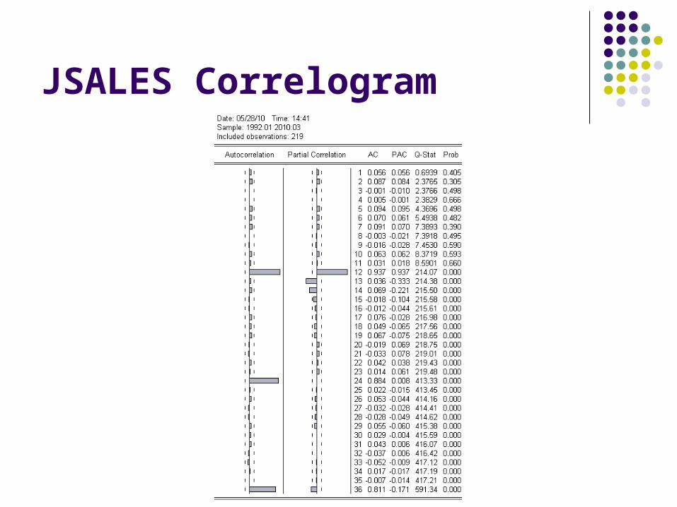
JSALES Correlogram
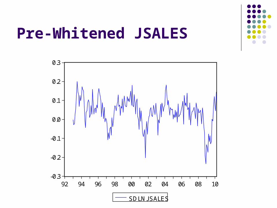
Pre-Whitened JSALES
-0.3
-0.2
-0.1
0.0
0.1
0.2
0.3
92 94 96 98 00 02 04 06 08 10
SDLNJSALES

SDLNJSALES
0
10
20
30
40
50
-0.2 -0.1 0.0 0.1 0.2
Series: SDLNJSALESSample 1993:01 2010:03Observations 207
Mean 0.038301Median 0.048112Maximum 0.200323Minimum -0.234369Std. Dev. 0.073908Skewness -0.809307Kurtosis 4.189813
Jarque-Bera 34.80675Probability 0.000000
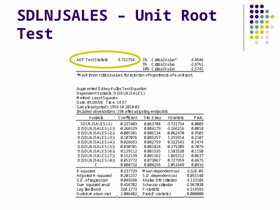
SDLNJSALES – Unit Root Test
ADF Test Statistic -3.721754 1% Critical Value* -3.4646 5% Critical Value -2.8761 10% Critical Value -2.5745
*MacKinnon critical values for rejection of hypothesis of a unit root.
Augmented Dickey-Fuller Test Equation Dependent Variable: D(SDLNJSALES) Method: Least Squares Date: 05/28/10 Time: 14:57 Sample(adjusted): 1993:10 2010:03 Included observations: 198 after adjusting endpoints
Variable Coefficient Std. Error t-Statistic Prob.
SDLNJSALES(-1) -0.237403 0.063788 -3.721754 0.0003 D(SDLNJSALES(-1)) -0.266529 0.084179 -3.166216 0.0018 D(SDLNJSALES(-2)) -0.005381 0.086134 -0.062470 0.9503 D(SDLNJSALES(-3)) 0.107076 0.085257 1.255914 0.2107 D(SDLNJSALES(-4)) 0.026693 0.082759 0.322543 0.7474 D(SDLNJSALES(-5)) -0.030701 0.081824 -0.375209 0.7079 D(SDLNJSALES(-6)) 0.129112 0.081535 1.583520 0.1150 D(SDLNJSALES(-7)) 0.152139 0.081562 1.865312 0.0637 D(SDLNJSALES(-8)) 0.053772 0.073867 0.727959 0.4675
C 0.008732 0.004256 2.051649 0.0416
R-squared 0.237729 Mean dependent var 6.52E-05 Adjusted R-squared 0.201237 S.D. dependent var 0.055148 S.E. of regression 0.049288 Akaike info criterion -3.133104 Sum squared resid 0.456702 Schwarz criterion -2.967030 Log likelihood 320.1773 F-statistic 6.514593 Durbin-Watson stat 2.006402 Prob(F-statistic) 0.000000
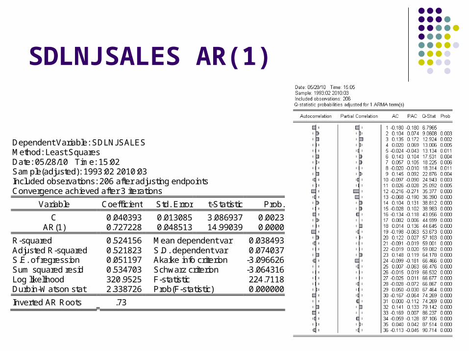
SDLNJSALES AR(1)
Dependent Variable: SDLNJSALES Method: Least Squares Date: 05/28/10 Time: 15:02 Sample(adjusted): 1993:02 2010:03 Included observations: 206 after adjusting endpoints Convergence achieved after 3 iterations
Variable Coefficient Std. Error t-Statistic Prob.
C 0.040393 0.013085 3.086937 0.0023 AR(1) 0.727228 0.048513 14.99039 0.0000
R-squared 0.524156 Mean dependent var 0.038493 Adjusted R-squared 0.521823 S.D. dependent var 0.074037 S.E. of regression 0.051197 Akaike info criterion -3.096626 Sum squared resid 0.534703 Schwarz criterion -3.064316 Log likelihood 320.9525 F-statistic 224.7118 Durbin-Watson stat 2.338726 Prob(F-statistic) 0.000000
Inverted AR Roots .73

SDLNJSALES ARMA(1,1)
Dependent Variable: SDLNJSALES Method: Least Squares Date: 05/28/10 Time: 15:08 Sample(adjusted): 1993:02 2010:03 Included observations: 206 after adjusting endpoints Convergence achieved after 8 iterations Backcast: 1993:01
Variable Coefficient Std. Error t-Statistic Prob.
C 0.042535 0.018240 2.332006 0.0207 AR(1) 0.869124 0.045764 18.99131 0.0000 MA(1) -0.314907 0.087689 -3.591189 0.0004
R-squared 0.553396 Mean dependent var 0.038493 Adjusted R-squared 0.548996 S.D. dependent var 0.074037 S.E. of regression 0.049721 Akaike info criterion -3.150334 Sum squared resid 0.501846 Schwarz criterion -3.101870 Log likelihood 327.4844 F-statistic 125.7705 Durbin-Watson stat 2.020548 Prob(F-statistic) 0.000000
Inverted AR Roots .87 Inverted MA Roots .31
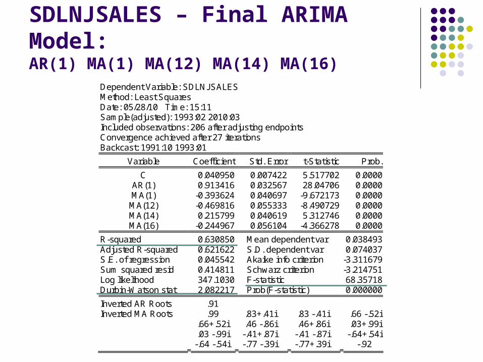
SDLNJSALES – Final ARIMA Model:AR(1) MA(1) MA(12) MA(14) MA(16)
Dependent Variable: SDLNJSALES Method: Least Squares Date: 05/28/10 Time: 15:11 Sample(adjusted): 1993:02 2010:03 Included observations: 206 after adjusting endpoints Convergence achieved after 27 iterations Backcast: 1991:10 1993:01
Variable Coefficient Std. Error t-Statistic Prob.
C 0.040950 0.007422 5.517702 0.0000 AR(1) 0.913416 0.032567 28.04706 0.0000 MA(1) -0.393624 0.040697 -9.672173 0.0000 MA(12) -0.469816 0.055333 -8.490729 0.0000 MA(14) 0.215799 0.040619 5.312746 0.0000 MA(16) -0.244967 0.056104 -4.366278 0.0000
R-squared 0.630850 Mean dependent var 0.038493 Adjusted R-squared 0.621622 S.D. dependent var 0.074037 S.E. of regression 0.045542 Akaike info criterion -3.311679 Sum squared resid 0.414811 Schwarz criterion -3.214751 Log likelihood 347.1030 F-statistic 68.35718 Durbin-Watson stat 2.082217 Prob(F-statistic) 0.000000
Inverted AR Roots .91 Inverted MA Roots .99 .83+.41i .83 -.41i .66 -.52i
.66+.52i .46 -.86i .46+.86i .03+.99i .03 -.99i -.41+.87i -.41 -.87i -.64+.54i -.64 -.54i -.77 -.39i -.77+.39i -.92

SDLNJSALES - Correlogram

SDLNJSALESSerial Correlation Test
Breusch-Godfrey Serial Correlation LM Test:
F-statistic 1.556660 Probability 0.187451 Obs*R-squared 5.289374 Probability 0.258873
Test Equation: Dependent Variable: RESID Method: Least Squares Date: 05/28/10 Time: 15:17
Variable Coefficient Std. Error t-Statistic Prob.
C -0.002718 0.007554 -0.359839 0.7194 AR(1) -0.013835 0.048035 -0.288021 0.7736 MA(1) 0.017865 0.048493 0.368409 0.7130 MA(12) 0.010197 0.057583 0.177081 0.8596 MA(14) -0.018825 0.048382 -0.389093 0.6976 MA(16) 0.013909 0.056199 0.247491 0.8048
RESID(-1) -0.047059 0.100407 -0.468681 0.6398 RESID(-2) 0.057479 0.084838 0.677507 0.4989 RESID(-3) 0.067851 0.081574 0.831772 0.4065 RESID(-4) -0.056304 0.079955 -0.704198 0.4821
R-squared 0.025677 Mean dependent var 0.003251 Adjusted R-squared -0.019063 S.D. dependent var 0.044865 S.E. of regression 0.045290 Akaike info criterion -3.304119 Sum squared resid 0.402039 Schwarz criterion -3.142571 Log likelihood 350.3242 F-statistic 0.573915 Durbin-Watson stat 2.018583 Prob(F-statistic) 0.817552
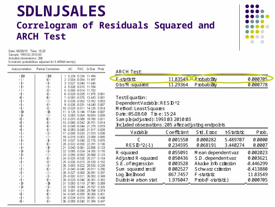
SDLNJSALESCorrelogram of Residuals Squared and ARCH Test
ARCH Test:
F-statistic 11.83549 Probability 0.000705 Obs*R-squared 11.29364 Probability 0.000778
Test Equation: Dependent Variable: RESID^2 Method: Least Squares Date: 05/28/10 Time: 15:24 Sample(adjusted): 1993:03 2010:03 Included observations: 205 after adjusting endpoints
Variable Coefficient Std. Error t-Statistic Prob.
C 0.001550 0.000282 5.489707 0.0000 RESID^2(-1) 0.234595 0.068191 3.440274 0.0007
R-squared 0.055091 Mean dependent var 0.002023 Adjusted R-squared 0.050436 S.D. dependent var 0.003621 S.E. of regression 0.003528 Akaike info criterion -8.446299 Sum squared resid 0.002527 Schwarz criterion -8.413880 Log likelihood 867.7457 F-statistic 11.83549 Durbin-Watson stat 1.976047 Prob(F-statistic) 0.000705
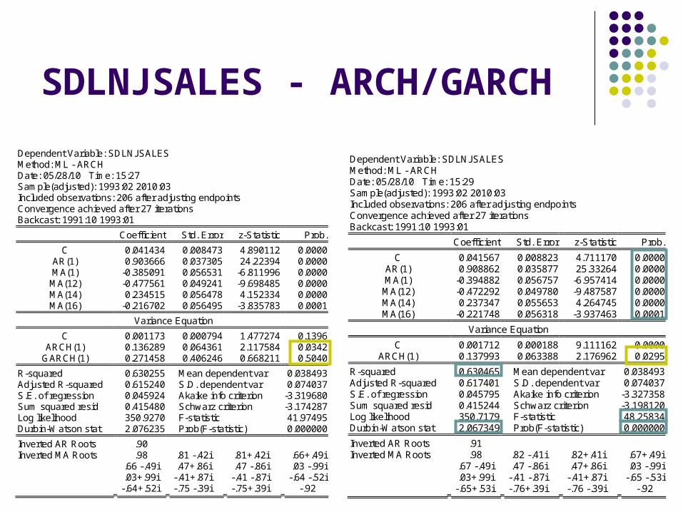
SDLNJSALES - ARCH/GARCH
Dependent Variable: SDLNJSALES Method: ML - ARCH Date: 05/28/10 Time: 15:27 Sample(adjusted): 1993:02 2010:03 Included observations: 206 after adjusting endpoints Convergence achieved after 27 iterations Backcast: 1991:10 1993:01
Coefficient Std. Error z-Statistic Prob.
C 0.041434 0.008473 4.890112 0.0000 AR(1) 0.903666 0.037305 24.22394 0.0000 MA(1) -0.385091 0.056531 -6.811996 0.0000 MA(12) -0.477561 0.049241 -9.698485 0.0000 MA(14) 0.234515 0.056478 4.152334 0.0000 MA(16) -0.216702 0.056495 -3.835783 0.0001
Variance Equation
C 0.001173 0.000794 1.477274 0.1396 ARCH(1) 0.136289 0.064361 2.117584 0.0342
GARCH(1) 0.271458 0.406246 0.668211 0.5040
R-squared 0.630255 Mean dependent var 0.038493 Adjusted R-squared 0.615240 S.D. dependent var 0.074037 S.E. of regression 0.045924 Akaike info criterion -3.319680 Sum squared resid 0.415480 Schwarz criterion -3.174287 Log likelihood 350.9270 F-statistic 41.97495 Durbin-Watson stat 2.076235 Prob(F-statistic) 0.000000
Inverted AR Roots .90 Inverted MA Roots .98 .81 -.42i .81+.42i .66+.49i
.66 -.49i .47+.86i .47 -.86i .03 -.99i .03+.99i -.41+.87i -.41 -.87i -.64 -.52i -.64+.52i -.75 -.39i -.75+.39i -.92
Dependent Variable: SDLNJSALES Method: ML - ARCH Date: 05/28/10 Time: 15:29 Sample(adjusted): 1993:02 2010:03 Included observations: 206 after adjusting endpoints Convergence achieved after 27 iterations Backcast: 1991:10 1993:01
Coefficient Std. Error z-Statistic Prob.
C 0.041567 0.008823 4.711170 0.0000 AR(1) 0.908862 0.035877 25.33264 0.0000 MA(1) -0.394882 0.056757 -6.957414 0.0000 MA(12) -0.472292 0.049780 -9.487587 0.0000 MA(14) 0.237347 0.055653 4.264745 0.0000 MA(16) -0.221748 0.056318 -3.937463 0.0001
Variance Equation
C 0.001712 0.000188 9.111162 0.0000 ARCH(1) 0.137993 0.063388 2.176962 0.0295
R-squared 0.630465 Mean dependent var 0.038493 Adjusted R-squared 0.617401 S.D. dependent var 0.074037 S.E. of regression 0.045795 Akaike info criterion -3.327358 Sum squared resid 0.415244 Schwarz criterion -3.198120 Log likelihood 350.7179 F-statistic 48.25834 Durbin-Watson stat 2.067349 Prob(F-statistic) 0.000000
Inverted AR Roots .91 Inverted MA Roots .98 .82 -.41i .82+.41i .67+.49i
.67 -.49i .47 -.86i .47+.86i .03 -.99i .03+.99i -.41 -.87i -.41+.87i -.65 -.53i -.65+.53i -.76+.39i -.76 -.39i -.92

Actual, Fitted, Residual
-0.2
-0.1
0.0
0.1
0.2
-0.3
-0.2
-0.1
0.0
0.1
0.2
0.3
94 96 98 00 02 04 06 08 10
Residual Actual Fitted

Histogram of Residuals
Non-normal, but single-peaked
0
5
10
15
20
25
30
-3 -2 -1 0 1 2 3
Series: Standardized Res idualsSample 1993:02 2010:03Observations 206
Mean 0.040591Median 0.072181Maximum 2.859502Minimum -3.353756Std. Dev . 1.000242Skewness -0.367183Kurtosis 3.733818
Jarque-Bera 9.250958Probability 0.009799

CorrelogramsStandardized Residuals Residuals Squared
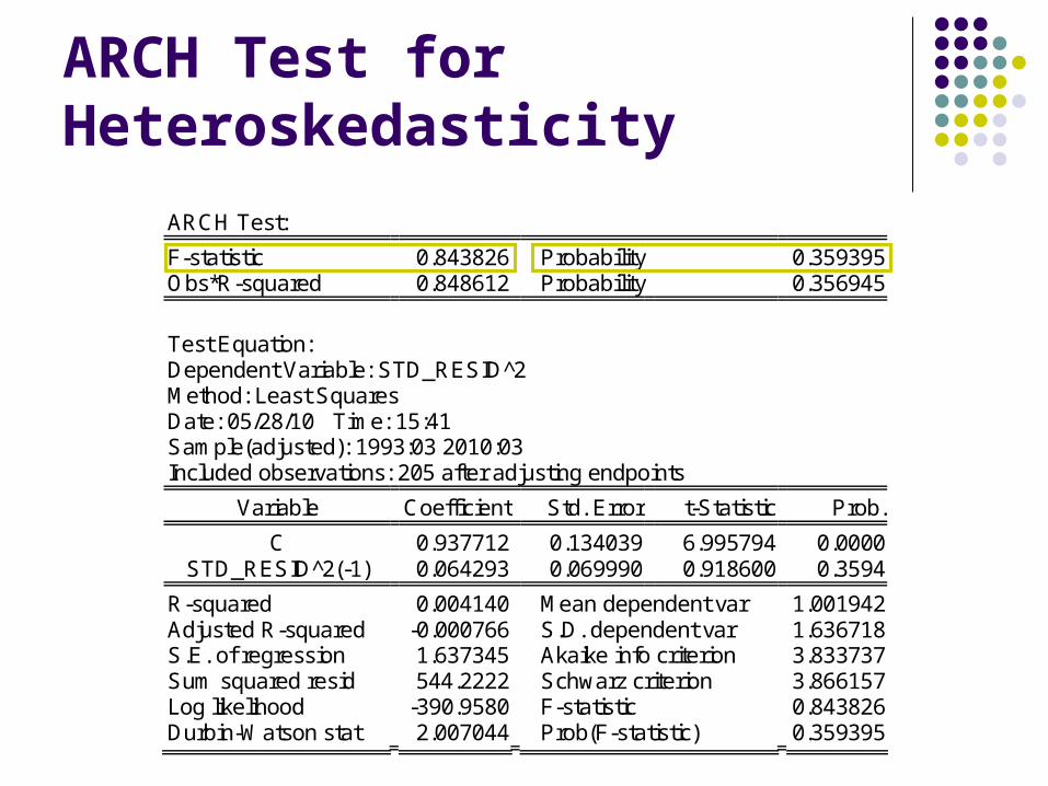
ARCH Test for Heteroskedasticity
ARCH Test:
F-statistic 0.843826 Probability 0.359395 Obs*R-squared 0.848612 Probability 0.356945
Test Equation: Dependent Variable: STD_RESID^2 Method: Least Squares Date: 05/28/10 Time: 15:41 Sample(adjusted): 1993:03 2010:03 Included observations: 205 after adjusting endpoints
Variable Coefficient Std. Error t-Statistic Prob.
C 0.937712 0.134039 6.995794 0.0000 STD_RESID^2(-1) 0.064293 0.069990 0.918600 0.3594
R-squared 0.004140 Mean dependent var 1.001942 Adjusted R-squared -0.000766 S.D. dependent var 1.636718 S.E. of regression 1.637345 Akaike info criterion 3.833737 Sum squared resid 544.2222 Schwarz criterion 3.866157 Log likelihood -390.9580 F-statistic 0.843826 Durbin-Watson stat 2.007044 Prob(F-statistic) 0.359395
Conclusion:
Accept the model!

Forecasting SDLNJSALES for Previous 12 Months
-0.3
-0.2
-0.1
0.0
0.1
0.2
0.3
06:01 06:07 07:01 07:07 08:01 08:07 09:01 09:07 10:01
SDLNJSALESFORECAST1
UPPERLOWER

Forecasting SDLNJSALES for Next 12 Months
-0.3
-0.2
-0.1
0.0
0.1
0.2
0.3
92 94 96 98 00 02 04 06 08 10
SDLNJSALESFORECAST2
UPPER2LOWER2
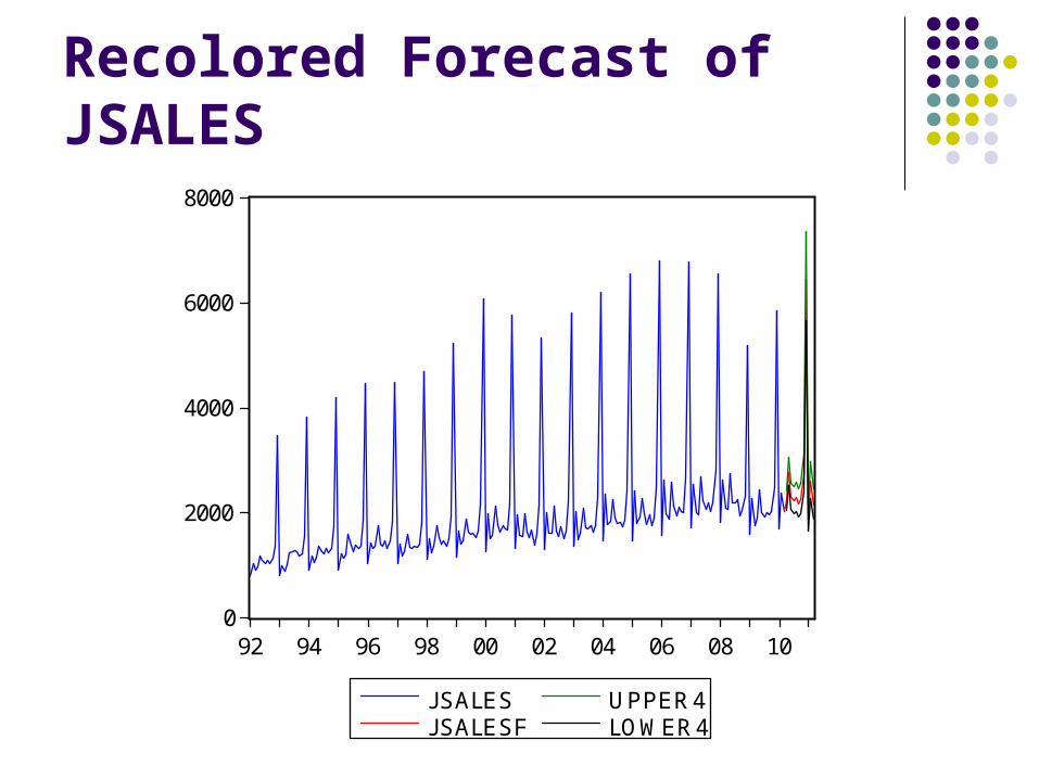
Recolored Forecast of JSALES
0
2000
4000
6000
8000
92 94 96 98 00 02 04 06 08 10
JSALESJSALESF
UPPER4LOWER4

Detailed Graph
1000
2000
3000
4000
5000
6000
7000
8000
05 06 07 08 09 10 11
JSALESJSALESF
UPPER4LOWER4

JSALES Data and Forecast
Actual values of U.S. Jewelry Sales from January, 2009 through March, 2010
Forecasted values from April, 2010 through March, 2011

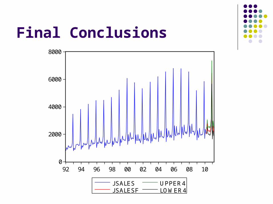
Final Conclusions
Forecasted recovery of Jewelry Sales for 2010 holiday season
10.35% increase predicted for December 2010 sales over 2009 levels
Upper bound of 95% confidence level predicts that, if everything goes very well, sales could be their highest since 1992
Final Conclusions
0
2000
4000
6000
8000
92 94 96 98 00 02 04 06 08 10
JSALESJSALESF
UPPER4LOWER4