Harri Turunen. Government spending in a volatile economy at the zero lower bound
45
Government spending in a volatile economy at the zero lower bound Harri Turunen University of Helsinki University of Cambridge February 16, 2015
-
Upload
eesti-pank -
Category
Economy & Finance
-
view
209 -
download
1
Transcript of Harri Turunen. Government spending in a volatile economy at the zero lower bound

Government spending in a volatile economy atthe zero lower bound
Harri Turunen
University of HelsinkiUniversity of Cambridge
February 16, 2015

Outline
Motivation
The model
Generalized Stochastic Simulation
Results

Outline
Motivation
The model
Generalized Stochastic Simulation
Results

Ramey (JEL 2011)
Reasonable people can argue, however, that the data donot reject 0.5 or 2.0.
I Blanchard & Perotti (2002): SVAR-identified tax shocksimply multiplier of 0.9 to 1.29
I Cogan, Cwik, Taylor & Wieland (2010): estimatedSmets-Wouters model implies 0.64 at peak

ECB refi rate, Fed Funds rate, BoJ overnight rate,2004-2014

Intuition on the multiplier at the ZLB
I Multiplier depends on response of hours worked to spendingincrease
I New Keynesian special case: when interest rates are low, themultiplier can be large
I With interest rates stuck, consumption level adjusted byworking more

This paper/presentation
I How does uncertainty affect the multiplier at the ZLB?
I Uncertainty modeled as stochastic volatility in governmentspending and aggregate productivity
I Model solved using a global method that accommodates theZLB
I Multipliers computed by simulating the model
I Not an explanation of causes of business cycles

What is spending uncertainty? What causes it?
Household uncertainty about government behavior
I Greek commitment to cuts and reforms (also in 2010!)
I U.S. government shutdown in 2013
More generally
I Uncertainty about a new party or politician
I Uncertainty about commitment
I Uncertainty about general economic conditions

Justiniano and Primiceri (AER 2008)DSGE-based estimate of volatility of U.S. government spending with confidence intervals

Baker et al (AER P&P 2014)Economic policy uncertainty index based on newspaper word count

Previous literature on multipliers at ZLB
I Christiano, Eichenbaum & Rebelo (2011): multiplier above 1in a linearized model
I Aruoba & Schorfheide (2013): multiplier greater than 1 - ifeconomy is in non-deflationary equilibrium
I Braun, Korber & Waki (2013): multiplier 1 or less, dependingon parametrization
I Fernandez-Villaverde, Gordon, Rubio-Ramirez &Guerron-Quintana (2013): above bound 0.6, at bound 1.5

My results
Volatility matters:
1. Spending volatility has a positive effect; high volatilityincreases the multiplier
2. Productivity volatility has a negative effect; high volatilitydecreases the multiplier
Different shocks can take the economy to the bound; the multiplierdepends on the shock
1. Shocks to discount rate result in large multipliers
2. Shocks to productivity yield small multipliers
3. Bond return shock and monetary policy shock in between
Size of spending increase strongly affects size of multiplier

Outline
Motivation
The model
Generalized Stochastic Simulation
Results

Model foundations
I Representative household
I Calvo pricing in production
I Central bank follows Taylor rule
I Government levies lump sum taxes and spends, has balancedbudget
I No capital, no distorting taxes

Shocks
I Discount rate (ut), labor preference (lt), bond return (bt),productivity (at), government spending (gt), monetary policy(rt)
I All follow ht = hρht−1 exp (σhεh,t), εh,t ∼ N (0, 1)
I Two volatility shocks: productivity (σa,t), governmentspending (σg ,t)
I log σj ,t = (1− %j) log σj + %j log σj ,t−1 + ςjηj ,t , ηj ,t ∼ N (0, 1)

Central bank
Nominal rate constrained by ZLB
Rt = max {1, φt}
Central bank follows Taylor rule:
φt = rtR1−ρ (Rt−1)ρ
[(πtπ∗
)φπ ( Yt
Y ∗
)φY ]1−ρDue to kink Rt non-differentiable =⇒ perturbation methodsinapplicable!

Spending
I Government borrows Bt , levies lump-sum taxes Tt and spends
I Budget always balanced
I Spending shock gt subject to stochastic volatility:
gt = gρgt−1 exp (σg ,tεg ,t)
log σg ,t = (1− %g ) log σg + %g log σg ,t−1 + ςgηg ,t
I Government expenditure computed as Gt = gtGYt

Households
Households consume final good Ct , supply labor Lt to intermediategoods producers, put savings into government bonds, maximize
maxCt ,Bt ,Lt
E0
∞∑t=0
βtut
[log (Ct)− lt
L1+ϑt
1 + ϑ
]
subject to
PtCt +Bt
bt≤ Rt−1Bt−1 + WtLt + Tt + Πt
Standard intertemporal optimality condition for bonds:
C−1t = βbtut
RtEt
[ut+1C
−1t+1
]In equilibrium
Ct =(1− gtG
)atLt∆t

Firms
I Competitive production of final good Yt using Dixit-Stiglitzaggregation
I Monopolistic production of intermediate goods with aggregateproductivity subject to stochastic volatility
I Calvo pricing implies optimality condition for reset prices Pt
Pt
Pt≡ St
Ft
where
St =ut ltat
Lϑt Yt + βθEt
[πεt+1St+1
]Ft = utC
−1t Yt + βθEt
[πε−1t+1Ft+1
]

Calibration
Objective of calibration: model hits the bound in roughly 6% ofperiods
I Shocks central: variances set to 0.005 in steady state,persistences 0.75, %a = %g = 0.9 and ςa = ςg = 0.1
I Central bank reacts strongly to inflation: φπ = 2, φY = 0.15,π∗ = 1.004 and ρ = 0.8
I Households: β = 0.994, ϑ = 1
I Firms: ε = 6, θ = 0.75

Outline
Motivation
The model
Generalized Stochastic Simulation
Results

Nutshell
I Approximate equilibrium conditions with polynomials of statevariables
I Polynomials found with fixed-point iteration:
1. Make a guess on parameters in polynomials
2. Simulate model for T periods using the polynomials
3. Regress “true” model outcomes on simulation outcome
4. Update guess using regression output. If no convergence, goto 2.

My implementation
I Third order polynomials for St , Ft and marginal utility
I Vector of state variablesXt = (∆t−1,Rt−1, at , bt , gt , lt , rt , ut , σa,t , σg ,t)
I Dimension of polynomials large - 286 parameters!
I Initial values from second-order perturbation of Gomme andKlein (2011)

Other technicalities
I Problem: regression coefficients unstable between iterations
I Solution: “stabilize” regression using singular valuedecomposition
I Use numerical integration to compute “true” model outcomesof expectations
I Iterate over structural parameters - even with stabilizationinvertibility issues arise
I 10-20 minutes per iteration

Outline
Motivation
The model
Generalized Stochastic Simulation
Results

Results
I Which shocks are important for hitting the bound?
I What happens at the bound to output and inflation?
I How large is the multiplier?

Which shocks drive the economy to the bound?Probability of hitting the bound after a shock in the next 10 periods at least once
Size of innov. at bt ut rt
2 s.d. 0.31 0.43 0.23 0.221 s.d. 0.28 0.34 0.24 0.230 s.d. 0.26 0.26 0.26 0.26-1 s.d. 0.24 0.2 0.28 0.28-2 s.d. 0.22 0.15 0.3 0.36
Legend: at productivity, bt bond return,ut discount rate, rt interest rate

Which shocks drive the economy to the bound?Realized and theoretical distributions of shocks at bound
-0.03 -0.02 -0.01 0 0.01 0.020
1
2
3x 10
4 Interest rate
-0.04 -0.02 0 0.02 0.040
1
2
3x 10
4 Bond premium
-0.04 -0.02 0 0.02 0.04 0.060
1
2
3x 10
4 Aggr. productivity
-0.04 -0.02 0 0.02 0.040
1
2
3x 10
4 Discount factor

Which shocks drive the economy to the bound?Realized and theoretical distributions of shocks at bound
-6.5 -6 -5.5 -5 -4.5 -40
1
2
3x 10
4 Vol. of productivity
-6.5 -6 -5.5 -5 -4.5 -40
1
2
3x 10
4 Vol. of spending
-0.04 -0.02 0 0.02 0.040
1
2
3x 10
4 Gov. spending
-0.04 -0.02 0 0.02 0.040
1
2
3x 10
4 Labor supply
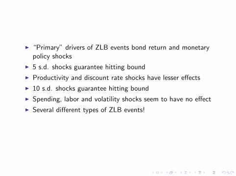
I “Primary” drivers of ZLB events bond return and monetarypolicy shocks
I 5 s.d. shocks guarantee hitting bound
I Productivity and discount rate shocks have lesser effects
I 10 s.d. shocks guarantee hitting bound
I Spending, labor and volatility shocks seem to have no effect
I Several different types of ZLB events!

Not all shocks are created equalImpulse responses to productivity and bond shocks that drive the economy to the ZLB
0 2 4 6 8 101
1.005
1.01
1.015
1.02
1.025
Agg
r. p
rodu
ct.
Output
0 2 4 6 8 100.98
0.985
0.99
0.995
1
1.005Inflation
0 2 4 6 8 100.94
0.96
0.98
1
Bon
d re
turn
0 2 4 6 8 100.97
0.98
0.99
1

Not all shocks are created equalImpulse responses to productivity and bond shocks that drive the economy to the ZLBtogether with a government intervention
0 2 4 6 8 101
1.005
1.01
1.015
1.02
1.025
Agg
r. p
rodu
ct.
Output
5 s.d. shock to spendingNo increase
0 2 4 6 8 100.98
0.985
0.99
0.995
1
1.005Inflation
0 2 4 6 8 100.94
0.96
0.98
1
Bon
d re
turn
0 2 4 6 8 100.97
0.98
0.99
1

Not all shocks are created equalImpulse responses to discount rate and monetary policy shocks that drive the economy tothe ZLB together with a government intervention
0 2 4 6 8 100.96
0.97
0.98
0.99
1
1.01
Dis
coun
t rat
e
Output
0 2 4 6 8 100.985
0.99
0.995
1
1.005Inflation
0 2 4 6 8 100.98
1
1.02
1.04
1.06
1.08
Inte
rest
rat
e
0 2 4 6 8 100.995
1
1.005
1.01
1.015

Simulation procedure for computing fiscal multipliers
1. Start from steady state. Hit the economy with a shock thatdrives it to the bound, a shock to volatility and a shock tospending.
2. Simulate 10 000 realizations for 10 periods.
3. Compute multiplier for period t as an average overrealizations with formula Yt−Yt∗
G1−G∗1
I Five cases: economy not at bound, at bound due toproductivity, discount rate, bond return or monetary shock
I Two volatility shocks: spending and productivity

Fiscal multiplier, not at boundVolatility in spending

Fiscal multiplier, not at boundVolatility in productivity
Productivity volatility shock
Sp
end
ing
sh
ock
-10 -5 0 5 10
20
15
10
5
1
0
0.5
1
1.5
2
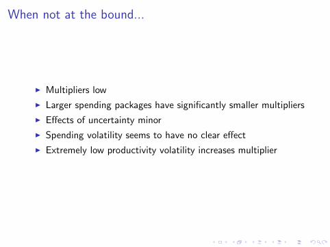
When not at the bound...
I Multipliers low
I Larger spending packages have significantly smaller multipliers
I Effects of uncertainty minor
I Spending volatility seems to have no clear effect
I Extremely low productivity volatility increases multiplier

Fiscal multiplier at ZLB1. Bond return shock
Spending volatility shock
Sp
end
ing
sh
ock
-10 -5 0 5 10
20
15
10
5
10.7
0.8
0.9
1
1.1
1.2
Productivity volatility shock
Sp
end
ing
sh
ock
-10 5 0 5 10
20
15
10
5
1 0.4
0.6
0.8
1
1.2
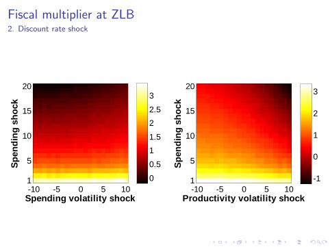
Fiscal multiplier at ZLB2. Discount rate shock
Spending volatility shock
Sp
end
ing
sh
ock
-10 -5 0 5 10
20
15
10
5
1 0
0.5
1
1.5
2
2.5
3
Productivity volatility shock
Sp
end
ing
sh
ock
-10 -5 0 5 10
20
15
10
5
1 -1
0
1
2
3

Some intuition
1. The economy is at the bound due to a high bond return shockor a low discount rate shock and there is a change inuncertainty
2. The government spends a portion of output greater thannormal
3. Households would like to save less, but the interest rate isstuck
From the household’s point of view, spending is taxation - thusuncertainty in spending is uncertainty in taxation

Fiscal multiplier at ZLB3. Monetary policy shock
Spending volatility shock
Sp
end
ing
sh
ock
-10 -5 0 5 10
20
15
10
5
1 0.2
0.4
0.6
0.8
1
1.2
Productivity volatility shock
Sp
end
ing
sh
ock
-10 -5 0 5 10
20
15
10
5
10
0.2
0.4
0.6
0.8
1
1.2

Fiscal multiplier at ZLB4. Productivity shock
Spending volatility shock
Sp
end
ing
sh
ock
-10 -5 0 5 10
20
15
10
5
1-0.5
0
0.5
Productivity volatility shock
Sp
end
ing
sh
ock
-10 -5 0 5 10
20
15
10
5
1
-1.5
-1
-0.5
0
0.5

Conclusions
I Size of the multiplier often, but not always, greater than 1,when the economy is at the ZLB
I Strong dependence on volatility: high spending volatility cansignificantly increase the multiplier
I Size of spending increase has a strong impact on multiplier
I Different shocks lead to different types of ZLB events anddifferent multipliers
I Caveats: lack of capital and distorting taxation probably skewresults