Handbook of Computational Social Choice - Ariel …procaccia.info/papers/comsoc.pdf · Handbook of...
554
HANDBOOK of COMPUTATIONAL SOCIAL CHOICE Felix Brandt Vincent Conitzer Ulle Endriss Jérôme Lang Ariel D. Procaccia EDITED BY
Transcript of Handbook of Computational Social Choice - Ariel …procaccia.info/papers/comsoc.pdf · Handbook of...

HANDBOOK of
COMPUTATIONALSOCIAL CHOICE
Felix Brandt Vincent Conitzer Ulle Endriss Jérôme Lang Ariel D. Procaccia
EDITED BY

Handbook of Computational Social Choice
The rapidly growing field of computational social choice, at the intersection of computerscience and economics, deals with the computational aspects of collective decision making.This handbook, written by thirty-six prominent members of the computational social choicecommunity, covers the field comprehensively. Chapters devoted to each of the field’s majorthemes offer detailed introductions. Topics include voting theory (such as the computa-tional complexity of winner determination and manipulation in elections), fair allocation(such as algorithms for dividing divisible and indivisible goods), coalition formation (suchas matching and hedonic games), and many more. Graduate students, researchers, and pro-fessionals in computer science, economics, mathematics, political science, and philosophywill benefit from this accessible and self-contained book.
Felix Brandt is Professor of Computer Science and Professor of Mathematics at TechnischeUniversitat Munchen.
Vincent Conitzer is the Kimberly J. Jenkins University Professor of New Technologies andProfessor of Computer Science, Professor of Economics, and Professor of Philosophy atDuke University.
Ulle Endriss is Associate Professor of Logic and Artificial Intelligence at the Institute forLogic, Language and Computation at the University of Amsterdam.
Jerome Lang is a senior researcher in computer science at CNRS-LAMSADE, UniversiteParis-Dauphine.
Ariel D. Procaccia is Assistant Professor of Computer Science at Carnegie MellonUniversity.


Handbook of ComputationalSocial Choice
Edited by
Felix BrandtTechnische Universitat Munchen
Vincent ConitzerDuke University
Ulle EndrissUniversity of Amsterdam
Jerome LangCNRS
Ariel D. ProcacciaCarnegie Mellon University
32 Avenue of the Americas, New York, NY 10013-2473, USA
Cambridge University Press is part of the University of Cambridge.
It furthers the University’s mission by disseminating knowledge in the pursuit ofeducation, learning, and research at the highest international levels of excellence.
www.cambridge.orgInformation on this title: www.cambridge.org/9781107060432
© Felix Brandt, Vincent Conitzer, Ulle Endriss, Jerome Lang, Ariel D. Procaccia 2016
This publication is in copyright. Subject to statutory exceptionand to the provisions of relevant collective licensing agreements,no reproduction of any part may take place without the writtenpermission of Cambridge University Press.
First published 2016
Printed in the United States of America
A catalog record for this publication is available from the British Library.
Library of Congress Cataloging in Publication Data
Handbook of computational social choice / edited by Felix Brandt, Technische UniversitatMunchen, Vincent Conitzer, Duke University, Ulle Endriss, University of Amsterdam, JeromeLang, CNRS, Ariel D. Procaccia, Carnegie Mellon University.
pages cmIncludes bibliographical references and index.ISBN 978-1-107-06043-2 (alk. paper)1. Social choice. 2. Interdisciplinary research. 3. Computer science. I. Brandt, Felix, 1973–editor.HB846.8.H33 2016302′.130285 – dc23 2015030289
Cambridge University Press has no responsibility for the persistence or accuracy of URLsfor external or third-party Internet Web sites referred to in this publication and does notguarantee that any content on such Web sites is, or will remain, accurate or appropriate.

Contents
Foreword page xiHerve Moulin
Contributors xiii
1 Introduction to Computational Social Choice 1Felix Brandt, Vincent Conitzer, Ulle Endriss, Jerome Lang,and Ariel D. Procaccia
1.1 Computational Social Choice at a Glance 11.2 History of Social Choice Theory 21.3 Book Outline 91.4 Further Topics 131.5 Basic Concepts in Theoretical Computer Science 17
Part I Voting
2 Introduction to the Theory of Voting 23William S. Zwicker
2.1 Introduction to an Introduction 232.2 Social Choice Functions: Plurality, Copeland, and Borda 262.3 Axioms I: Anonymity, Neutrality, and the Pareto Property 302.4 Voting Rules I: Condorcet Extensions, Scoring Rules, and Run-Offs 332.5 An Informational Basis for Voting Rules: Fishburn’s Classification 382.6 Axioms II: Reinforcement and Monotonicity Properties 392.7 Voting Rules II: Kemeny and Dodgson 442.8 Strategyproofness: Impossibilities 462.9 Strategyproofness: Possibilities 51
2.10 Approval Voting 532.11 The Future 56
v
vi contents
3 Tournament Solutions 57Felix Brandt, Markus Brill, and Paul Harrenstein
3.1 Introduction 573.2 Preliminaries 583.3 Common Tournament Solutions 623.4 Strategyproofness and Agenda Implementation 763.5 Generalizations to Weak Tournaments 813.6 Further Reading 83
4 Weighted Tournament Solutions 85Felix Fischer, Olivier Hudry, and Rolf Niedermeier
4.1 Kemeny’s Rule 864.2 Computing Kemeny Winners and Kemeny Rankings 884.3 Further Median Orders 944.4 Applications in Rank Aggregation 964.5 Other C2 Functions 96
5 Dodgson’s Rule and Young’s Rule 103Ioannis Caragiannis, Edith Hemaspaandra, and Lane A.Hemaspaandra
5.1 Overview 1035.2 Introduction, Election-System Definitions, and Results Overview 1035.3 Winner-Problem Complexity 1075.4 Heuristic Algorithms 1135.5 The Parameterized Lens 1155.6 Approximation Algorithms 1185.7 Bibliography and Further Reading 125
6 Barriers to Manipulation in Voting 127Vincent Conitzer and Toby Walsh
6.1 Introduction 1276.2 Gibbard-Satterthwaite and Its Implications 1286.3 Noncomputational Avenues around Gibbard-Satterthwaite 1296.4 Computational Hardness as a Barrier to Manipulation 1316.5 Can Manipulation Be Hard Most of the Time? 1396.6 Fully Game-Theoretic Models 1426.7 Conclusions 144
7 Control and Bribery in Voting 146Piotr Faliszewski and Jorg Rothe
7.1 Introduction 1467.2 Preliminaries 1477.3 Control 1497.4 Bribery 1597.5 A Positive Look 1677.6 Summary 168
8 Rationalizations of Voting Rules 169Edith Elkind and Arkadii Slinko
8.1 Introduction 1698.2 Consensus-Based Rules 170
contents vii
8.3 Rules as Maximum Likelihood Estimators 1848.4 Conclusions and Further Reading 195
9 Voting in Combinatorial Domains 197Jerome Lang and Lirong Xia
9.1 Motivations and Classes of Problems 1979.2 Simultaneous Voting and the Separability Issue 2009.3 Approaches Based on Completion Principles 2049.4 Sequential Voting 2159.5 Concluding Discussion 221
10 Incomplete Information and Communication in Voting 223Craig Boutilier and Jeffrey S. Rosenschein10.1 Introduction 22310.2 Models of Partial Preferences 22410.3 Solution Concepts with Partial Preferences 22710.4 Communication and Query Complexity 23410.5 Preference Elicitation 23910.6 Voting with an Uncertain Set of Alternatives 24410.7 Compilation Complexity 24710.8 Social Choice from a Utilitarian Perspective 25010.9 Conclusions and Future Directions 256
Part II Fair Allocation
11 Introduction to the Theory of Fair Allocation 261William Thomson11.1 Introduction 26111.2 What Is a Resource Allocation Problem? 26311.3 Solutions and Rules 26811.4 A Sample of Results 27711.5 Conclusion 282
12 Fair Allocation of Indivisible Goods 284Sylvain Bouveret, Yann Chevaleyre, and Nicolas Maudet12.1 Preferences for Resource Allocation Problems 28612.2 The Fairness versus Efficiency Trade-Off 29412.3 Computing Fair Allocations 29812.4 Protocols for Fair Allocation 30412.5 Conclusion 309
13 Cake Cutting Algorithms 311Ariel D. Procaccia13.1 Introduction 31113.2 The Model 31113.3 Classic Cake Cutting Algorithms 31313.4 Complexity of Cake Cutting 31613.5 Optimal Cake Cutting 32313.6 Bibliography and Further Reading 328

viii contents
Part III Coalition Formation
14 Matching under Preferences 333Bettina Klaus, David F. Manlove, and Francesca Rossi14.1 Introduction and Discussion of Applications 33314.2 Two-Sided Preferences 33614.3 One-Sided Preferences 34514.4 Concluding Remarks and Further Reading 354
15 Hedonic Games 356Haris Aziz and Rahul Savani15.1 Introduction 35615.2 Solution Concepts 35915.3 Preference Restrictions and Game Representations 36115.4 Algorithms and Computational Complexity 36715.5 Further Reading 373
16 Weighted Voting Games 377Georgios Chalkiadakis and Michael Wooldridge16.1 Introduction 37716.2 Basic Definitions 37816.3 Basic Computational Properties 38316.4 Voter Weight versus Voter Power 38816.5 Simple Games and Yes/No Voting Systems 39016.6 Conclusions 39416.7 Further Reading 394
Part IV Additional Topics
17 Judgment Aggregation 399Ulle Endriss17.1 Introduction 39917.2 Basics 40217.3 Aggregation Rules 40717.4 Agenda Characterization Results 41417.5 Related Frameworks 42117.6 Applications in Computer Science 42317.7 Bibliographic Notes and Further Reading 424
18 The Axiomatic Approach and the Internet 427Moshe Tennenholtz and Aviv Zohar18.1 Introduction 42718.2 An Axiomatic Characterization of PageRank 42918.3 Trust-Based Recommendations 43518.4 Mechanisms for Multilevel Marketing 44118.5 Discussion: Additional Applications 450
19 Knockout Tournaments 453Virginia Vassilevska Williams19.1 Introduction 45319.2 Formal Definition and Some Properties 454

contents ix
19.3 Agenda Control for General Knockout Tournaments 45619.4 Agenda Control for Balanced Trees Is Easy for Special Instances 46319.5 Extensions and Further Reading 471
References 475Index 529

Foreword
Herve Moulin
Axiomatics and algorithmics are two methodologies at the forefront of modern mathe-matics. The latter goes back to the very birth of mathematics, whereas the former wasnot developed until Hilbert’s famous contributions in the late 1800s.
Yet the axiomatic approach was the first to appear in modern social sciences, throughthe instant success in 1951 of K. Arrow’s Social Choice and Individual Values. Beyondthe negative, discouraging message of its famous (im)possibility theorem, that bookhad an immensely positive influence on the development of mathematical economics.It opened the way to the critical evaluation of actual democratic institutions throughthe filter of “self-evident” normative principles. Conversely, it allowed us to define“optimal” rules for collective decision making and/or the allocation of scarce resourcesby the convergence of a collection of such principles. In short, it started the field ofmechanism design.
Cake division is probably the first instance of an economic model with an algorith-mic twist. The mathematical statement of the problem goes back to B. Knaster andH. Steinhaus in the 1940s: it combines the normative choice of fairness axioms withthe algorithmic concern for a protocol made of simple “cut and choose” operations.This literature did not have noticeable influence on the exponential development ofmechanism design in the last 40 years, in part because it was developed mostly bymathematicians. Computational social choice will, I believe, bring it out from its rela-tive obscurity.
In less than two decades, the COMSOC community has generated an intense dia-logue between economists working on the normative side of mechanism design andcomputer scientists poised to test the computational complexity of these mechanisms. Aremarkable side product of this collaboration is clear from the choice of the 19 thoroughchapters. Under a common axiomatic and computational umbrella, they discuss
� the social choice problem of selecting a public outcome from the conflicting opinionsof the citizens
� the microeconomic problem of dividing private commodities fairly and efficiently whenindividual preferences differ
xi

xii foreword
� the market design problem of (bilaterally) matching employees to firms, students toschools, and so on
� the design of reputation indices and ranking methods in peer-to-peer systems such asthe Internet
� the formation and stability of “local public goods,” that is, (hedonic) coalitions of agentswith common interests
The relative weights of these problems are naturally quite unequal, but the point is theircoexistence.
The book offers to noneconomists an outstanding self-contained introduction tonormative themes in contemporary economics and to economists a thorough discussionof the computational limits of their art. But I also recommend it to anyone with a tastefor axiomatics: it is replete with new and open questions that will be with us for sometime.

Contributors
Haris Aziz NICTA and University of New South Wales, Sydney, Australia
Craig Boutilier Department of Computer Science, University of Toronto, Canada
Sylvain Bouveret Laboratoire d’Informatique de Grenoble, Universite Grenoble-Alpes, France
Felix Brandt Institut fur Informatik, Technische Universitat Munchen, Germany
Markus Brill Department of Computer Science, Duke University, United States ofAmerica
Ioannis Caragiannis Department of Computer Engineering and Informatics, Univer-sity of Patras, Greece
Georgios Chalkiadakis School of Electronic and Computer Engineering, TechnicalUniversity of Crete, Greece
Yann Chevaleyre Laboratoire d’Informatique de Paris Nord, Universite Paris-Nord,France
Vincent Conitzer Department of Computer Science, Duke University, United Statesof America
Edith Elkind Department of Computer Science, University of Oxford, UnitedKingdom
Ulle Endriss Institute for Logic, Language and Computation (ILLC), University ofAmsterdam, The Netherlands
Piotr Faliszewski Katedra Informatyki, AGH University of Science and Technology,Poland
Felix Fischer Statistical Laboratory, University of Cambridge, United Kingdom
xiii
xiv contributors
Paul Harrenstein Department of Computer Science, University of Oxford, UnitedKingdom
Edith Hemaspaandra Department of Computer Science, Rochester Institute of Tech-nology, United States of America
Lane A. Hemaspaandra Department of Computer Science, University of Rochester,United States of America
Olivier Hudry Institut Mines-Telecom, Telecom ParisTech and CNRS, France
Bettina Klaus Faculty of Business and Economics, University of Lausanne,Switzerland
Jerome Lang Laboratoire d’Analyse et Modelisation de Systemes pour l’Aide a laDecision (LAMSADE), CNRS and Universite Paris-Dauphine, France
David F. Manlove School of Computing Science, University of Glasgow, UnitedKingdom
Nicolas Maudet Sorbonne Universites, UPMC Univ. Paris 06, CNRS, LIP6 UMR7606, France
Rolf Niedermeier Fakultat Elektrotechnik und Informatik, Technische UniversitatBerlin, Germany
Ariel D. Procaccia Computer Science Department, Carnegie Mellon University,United States of America
Jeffrey S. Rosenschein School of Computer Science and Engineering, The HebrewUniversity of Jerusalem, Israel
Francesca Rossi Department of Mathematics, University of Padova, Italy
Jorg Rothe Institut fur Informatik, Heinrich-Heine-Universitat Dusseldorf,Germany
Rahul Savani Department of Computer Science, University of Liverpool, UnitedKingdom
Arkadii Slinko Department of Mathematics, University of Auckland, New Zealand
Moshe Tennenholtz Faculty of Industrial Engineering and Management, Technion–Israel Institute of Technology, Israel
William Thomson Department of Economics, University of Rochester, United Statesof America
Toby Walsh University of New South Wales and NICTA, Sydney, Australia
Virginia Vassilevska Williams Computer Science Department, Stanford University,United States of America
Michael Wooldridge Department of Computer Science, University of Oxford, UnitedKingdom

contributors xv
Lirong Xia Computer Science Department, Rensselaer Polytechnic Institute, UnitedStates of America
Aviv Zohar School of Computer Science and Engineering, The Hebrew University ofJerusalem, Israel
William S. Zwicker Department of Mathematics, Union College, United States ofAmerica

CHAPTER 1
Introduction to ComputationalSocial Choice
Felix Brandt, Vincent Conitzer, Ulle Endriss,Jerome Lang, and Ariel D. Procaccia
1.1 Computational Social Choice at a Glance
Social choice theory is the field of scientific inquiry that studies the aggregation of indi-vidual preferences toward a collective choice. For example, social choice theorists—who hail from a range of different disciplines, including mathematics, economics,and political science—are interested in the design and theoretical evaluation of votingrules. Questions of social choice have stimulated intellectual thought for centuries.Over time, the topic has fascinated many a great mind, from the Marquis de Condorcetand Pierre-Simon de Laplace, through Charles Dodgson (better known as Lewis Car-roll, the author of Alice in Wonderland), to Nobel laureates such as Kenneth Arrow,Amartya Sen, and Lloyd Shapley.
Computational social choice (COMSOC), by comparison, is a very young field thatformed only in the early 2000s. There were, however, a few precursors. For instance,David Gale and Lloyd Shapley’s algorithm for finding stable matchings between twogroups of people with preferences over each other, dating back to 1962, truly had acomputational flavor. And in the late 1980s, a series of papers by John Bartholdi, CraigTovey, and Michael Trick showed that, on the one hand, computational complexity,as studied in theoretical computer science, can serve as a barrier against strategicmanipulation in elections, but on the other hand, it can also prevent the efficient use ofsome voting rules altogether. Around the same time, a research group around BernardMonjardet and Olivier Hudry also started to study the computational complexity ofpreference aggregation procedures.
Assessing the computational difficulty of determining the output of a voting rule,or of manipulating it, is a wonderful example of the importation of a concept fromone field, theoretical computer science, to what at that time was still considered anentirely different one, social choice theory. It is this interdisciplinary view on collectivedecision making that defines computational social choice as a field. But, importantly,the contributions of computer science to social choice theory are not restricted to thedesign and analysis of algorithms for preexisting social choice problems. Rather, thearrival of computer science on the scene led researchers to revisit the old problem of
1
2 1 introduction to computational social choice
social choice from scratch. It offered new perspectives, and it led to many new typesof questions, thereby arguably contributing significantly to a revival of social choicetheory as a whole.
Today, research in computational social choice has two main thrusts. First,researchers seek to apply computational paradigms and techniques to provide a betteranalysis of social choice mechanisms, and to construct new ones. Leveraging the the-ory of computer science, we see applications of computational complexity theory andapproximation algorithms to social choice. Subfields of artificial intelligence, such asmachine learning, reasoning with uncertainty, knowledge representation, search, andconstraint reasoning, have also been applied to the same end.
Second, researchers are studying the application of social choice theory to compu-tational environments. For example, it has been suggested that social choice theorycan provide tools for making joint decisions in multiagent system populated by het-erogeneous, possibly selfish, software agents. Moreover, it is finding applications ingroup recommendation systems, information retrieval, and crowdsourcing. Althoughit is difficult to change a political voting system, such low-stake environments allowthe designer to freely switch between choice mechanisms, and therefore they providean ideal test bed for ideas coming from social choice theory.
This book aims to provide an authoritative overview of the field of computationalsocial choice. It has been written for students and scholars from both computer sci-ence and economics, as well as for others from the mathematical and social sciencesmore broadly. To position the field in its wider context, in Section 1.2, we provide abrief review of the history of social choice theory. The structure of the book reflectsthe internal structure of the field. We provide an overview of this structure by brieflyintroducing each of the remaining 18 chapters of the book in Section 1.3. As compu-tational social choice is still rapidly developing and expanding in scope every year,naturally, the coverage of the book cannot be exhaustive. Section 1.4 therefore brieflyintroduces a number of important active areas of research that, at the time of conceivingthis book, were not yet sufficiently mature to warrant their own chapters. Section 1.5,finally, introduces some basic concepts from theoretical computer science, notably thefundamentals of computational complexity theory, with which some readers may notbe familiar.
1.2 History of Social Choice Theory
Modern research in computational social choice builds on a long tradition of work oncollective decision making. We can distinguish three periods in the study of collectivedecision making: early ideas regarding specific rules going back to antiquity; theclassical period, witnessing the development of a general mathematical theory of socialchoice in the second half of the twentieth century; and the “computational turn” of thevery recent past. We briefly review each of these three periods by providing a smallselection of illustrative examples.
1.2.1 Early Ideas: Rules and Paradoxes
Collective decision-making problems come in many forms. They include the questionof how to fairly divide a set of resources, how to best match people on the basis of their
1 .2 history of social choice theory 3
preferences, and how to aggregate the beliefs of several individuals. The paradigmaticexample, however, is voting: how should we aggregate the individual preferences ofseveral voters over a given set of alternatives so as to be able to choose the “best”alternative for the group? This important question has been pondered by a number ofthinkers for a long time. Also the largest part of this book, Part I, is devoted to voting.We therefore start our historic review of social choice theory with a discussion of earlyideas pertaining to voting.1
Our first example for the discussion of a problem in voting goes back to Romantimes. Pliny the Younger, a Roman senator, described in a.d. 105 the following problemin a letter to an acquaintance. The Senate had to decide on the fate of a number ofprisoners: acquittal (A), banishment (B), or condemnation to death (C). Althoughoption A, favored by Pliny, had the largest number of supporters, it did not have anabsolute majority. One of the proponents of harsh punishment then strategically movedto withdraw proposal C, leaving its former supporters to rally behind option B, whicheasily won the majority contest between A and B. Had the senators voted on all threeoptions, using the plurality rule (under which the alternative ranked at the top by thehighest number of voters wins), option A would have won. This example illustratesseveral interesting features of voting rules. First, it may be interpreted as demonstratinga lack of fairness of the plurality rule: even though a majority of voters believes A tobe inferior to one of the other options (namely, B), A still wins. This and other fairnessproperties of voting rules are reviewed in Chapter 2. Second, Pliny’s anecdote is aninstance of what nowadays is called election control by deleting candidates. By deletingC, Pliny’s adversary in the senate was able to ensure that B rather than A won theelection. Such control problems, particularly their algorithmic aspects, are discussedin Chapter 7. Third, the example also illustrates the issue of strategic manipulation.Even if option C had not been removed, the supporters of C could have manipulatedthe election by pretending that they supported B rather than C, thereby ensuring apreferred outcome, namely, B rather than A. Manipulation is discussed in depth inChapters 2 and 6.
In the Middle Ages, the Catalan philosopher, poet, and missionary Ramon Llull(1232–1316) discussed voting rules in several of his writings. He supported the ideathat election outcomes should be based on direct majority contests between pairs ofcandidates. Such voting rules are discussed in detail in Chapter 3. What exact rule hehad in mind cannot be unambiguously reconstructed anymore, but it may have beenthe rule that today is known as the Copeland rule, under which the candidate who winsthe largest number of pairwise majority contests is elected. Whereas Pliny specificallydiscussed the subjective interests of the participants, Llull saw voting as a means ofrevealing the divine truth about who is the objectively best candidate, for example,to fill the position of abbess in a convent. The mathematical underpinnings of thisepistemic perspective on voting are discussed in Chapter 8.
Our third example is taken from the period of the Enlightenment. The works ofthe French engineer Jean-Charles de Borda (1733–1799) and the French philosopherand mathematician Marie Jean Antoine Nicolas de Caritat (1743–1794), better known
1 There are also instances of very early writings on other aspects of social choice. A good example is the discussionof fair division problems in the Talmud, as noted and analyzed in modern terms by game theorists Aumann andMaschler (1985).

4 1 introduction to computational social choice
as the Marquis de Condorcet—and particularly the lively dispute between them—arewidely regarded as the most significant contributions to social choice theory in the earlyperiod of the field. In 1770, Borda proposed a method of voting, today known as theBorda rule, under which each voter ranks all candidates, and each candidate receivesas may points from a given voter as that voter ranks other candidates below her. Heargued for the superiority of his rule over the plurality rule by discussing an examplesimilar to that of Pliny, where the plurality winner would lose in a direct majoritycontest to another candidate, while the Borda winner does not have that deficiency. ButCondorcet argued against Borda’s rule on very similar grounds. Consider the followingscenario with 3 candidates and 11 voters, which is a simplified version of an exampleCondorcet described in 1788:
4 3 2 2
Peter Paul Paul JamesPaul James Peter Peter
James Peter James Paul
In this example, four voters prefer candidate Peter over candidate Paul, whom theyprefer over candidate James, and so forth. Paul wins this election both under the pluralityrule (with 3 + 2 = 5 points) and the Borda rule (with 4 · 1 + 3 · 2 + 2 · 2 + 2 · 0 = 14points). However, a majority of voters (namely, 6 out of 11) prefer Peter to Paul. Infact, Peter also wins against James in a direct majority contest, so there arguably is avery strong case for rejecting voting rules that would not elect Peter in this situation.In today’s terminology, we call Peter the Condorcet winner.
Now suppose two additional voters join the election, who both prefer James, toPeter, to Paul. Then a majority prefers Peter to Paul, and a majority prefers Paul toJames, but now also a majority prefers James to Peter. This, the fact that the majoritypreference relation may turn out to be cyclic, is known as the Condorcet paradox. Itshows that Condorcet’s proposal, to be guided by the outcomes of pairwise majoritycontests, does not always lead to a clear election outcome.
In the nineteenth century, the British mathematician and story teller Charles Dodgson(1832–1898), although believed to have been unaware of Condorcet’s work, suggesteda voting rule designed to circumvent this difficulty. In cases where there is a singlecandidate who beats every other candidate in pairwise majority contests, he proposedto elect that candidate (the Condorcet winner). In all other cases, he proposed to counthow many elementary changes to the preferences of the voters would be required beforea given candidate would become the Condorcet winner, and to elect the candidate forwhich the required number of changes is minimal. In this context, he considered theswap of two candidates occurring adjacently in the preference list of a voter as such anelementary change. The Dodgson rule is analyzed in detail in Chapter 5.
This short review, it is hoped, gives the reader some insight into the kinds of questionsdiscussed by the early authors. The first period in the history of social choice theory isreviewed in depth in the fascinating collection edited by McLean and Urken (1995).
1.2.2 Classical Social Choice Theory
While early work on collective decision making was limited to the design of specificrules and on finding fault with them in the context of specific examples, around the
1 .2 history of social choice theory 5
middle of the twentieth century, the focus suddenly changed. This change was due tothe seminal work of Kenneth Arrow, who, in 1951, demonstrated that the problem withthe majority rule highlighted by the Condorcet paradox is in fact much more general.Arrow proved that there exists no reasonable preference aggregation rule that doesnot violate at least one of a short list of intuitively appealing requirements (Arrow,1951). That is, rather than proposing a new rule or pointing out a specific problem withan existing rule, Arrow developed a mathematical framework for speaking about andanalyzing all possible such rules.
Around the same time, in related areas of economic theory, Nash (1950) publishedhis seminal paper on the bargaining problem, which is relevant to the theory of fair allo-cation treated in Part II of this book, and Shapley (1953) published his groundbreakingpaper on the solution concept for cooperative games now carrying his name, whichplays an important role in coalition formation, to which Part III of this book is devoted.What all of these classical papers have in common is that they specified philosophicallyor economically motivated requirements in mathematically precise terms, as so-calledaxioms, and then rigorously explored the logical consequences of these axioms. As anexample of this kind of axiomatic work of this classical period, let us review Arrow’sresult in some detail.
Let N = {1, . . . , n} be a finite set of individuals (or voters, or agents), and letA be a finite set of alternatives (or candidates). The set of all weak orders � onA, that is, the set of all binary relations on A that are complete and transitive, isdenoted as R(A), and the set of all linear orders � on A, which in addition areantisymmetric, is denoted as L(A). In both cases, we use � to denote the strict partof �. We use weak orders to model preferences over alternatives that permit ties andlinear orders to model strict preferences. A social welfare function (SWF) is a functionof the form f : L(A)n → R(A). That is, f is accepting as input a so-called profileP = (�1, . . . ,�n) of preferences, one for each individual, and maps it to a singlepreference order, which we can think of as representing a suitable compromise. Weallow ties in the output, but not in the individual preferences. When f is clear from thecontext, we write � for f (�1, . . . ,�n), the outcome of the aggregation, and refer to itas the social preference order.
Arrow argued that any reasonable SWF should be weakly Paretian and independentof irrelevant alternatives (IIA). An SWF f is weakly Paretian if, for any two alternativesa, b ∈ A, it is the case that, if a �i b for all individuals i ∈ N , then also a � b. Thatis, if everyone strictly prefers a to b, then also the social preference order should ranka strictly above b. An SWF f is IIA if, for any two alternatives a, b ∈ A, the relativeranking of a and b by the social preference order � only depends on the relativerankings of a and b provided by the individuals—but not, for instance, on how theindividuals rank some third alternative c. To understand that it is not straightforwardto satisfy these two axioms, observe that, for instance, the SWF that ranks alternativesin the order of frequency with which they appear in the top position of an individualpreference is not IIA, and that the SWF that simply declares all alternatives as equallypreferable is not Paretian. The majority rule, while easily seen to be both Paretian andIIA, is not an SWF, because it does not always return a weak order, as the Condorcetparadox has shown.
An example of an SWF that most people would consider rather unreasonable isa dictatorship. We say that the SWF f is a dictatorship if there exists an individual
6 1 introduction to computational social choice
i� ∈ N (the dictator) such that, for all alternatives a, b ∈ A, it is the case that a �i� b
implies a � b. Thus, f simply copies the (strict) preferences of the dictator, whateverthe preferences of the other individuals. Now, it is not difficult to see that everydictatorship is both Paretian and IIA. The surprising—if not outright disturbing—resultdue to Arrow is that the converse is true as well:
Theorem 1.1 (Arrow, 1951). When there are three or more alternatives, then everySWF that is weakly Paretian and IIA must be a dictatorship.
Proof. Suppose |A| � 3, and let f be any SWF that is weakly Paretian and IIA. Forany profile P and alternatives a, b ∈ A, let NP
a�b ⊆ N denote the set of individualswho rank a strictly above b in P . We call a coalition C ⊆ N of individuals a decisivecoalition for alternative a versus alternative b if NP
a�b ⊇ C implies a � b, that is,if everyone in C ranking a strictly above b is a sufficient condition for the socialpreference order to do the same. Thus, to say that f is weakly Paretian is the same asto say that the grand coalition N is decisive, and to say that f is dictatorial is the sameas to say that there exists a singleton that is decisive. We call C weakly decisive for a
vs. b if we have at least that NPa�b = C implies a � b.
We first show that C being weakly decisive for a versus b implies C being (not justweakly) decisive for all pairs of alternatives. This is sometimes called the ContagionLemma or the Field Expansion Lemma. So let C be weakly decisive for a versus b.We show that C is also decisive for a′ versus b′. We do so under the assumption thata, b, a′, b′ are mutually distinct (the other cases are similar). Consider any profile P
such that a′ �i a �i b �i b′ for all i ∈ C, and a′ �j a, b �j b′, and b �j a for allj �∈ C. Then, from weak decisiveness of C for a versus b we get a � b; from f beingweakly Paretian, we get a′ � a and b � b′, and thus from transitivity, we get a′ � b′.Hence, in the specific profile P considered, the members of C ranking a′ above b′ wassufficient for a′ getting ranked above b′ also in the social preference order. But notethat, first, we did not have to specify how individuals outside of C rank a′ versus b′, andthat, second, due to f being IIA, the relative ranking of a′ versus b′ can only dependon the individual rankings of a′ versus b′. Hence, the only part of our construction thatactually mattered was that everyone in C ranked a′ above b′. So C really is decisivefor a′ versus b′ as claimed.
Consider any coalition C ⊆ N with |C| � 2 that is decisive (for some pair ofalternatives, and thus for all pairs). Next, we will show that we can always split C
into two nonempty subsets C1, C2 with C1 ∪ C2 = C and C1 ∩ C2 = ∅ such that oneof C1 and C2 is decisive for all pairs as well. This is sometimes called the SplittingLemma or the Group Contraction Lemma. Recall that |A| � 3. Consider a profile P inwhich everyone ranks alternatives a, b, c in the top three positions and, furthermore,a �i b �i c for all i ∈ C1, b �j c �j a for all j ∈ C2, and c �k a �k b for all k �∈C1 ∪ C2. As C = C1 ∪ C2 is decisive, we certainly get b � c. By completeness, wemust have either a � c or c � a. In the first case, we have a situation where exactlythe individuals in C1 rank a above c and in the social preference order a also is rankedabove c. Thus, due to f being IIA, in every profile where exactly the individuals in C1
rank a above c, a will come out above c. That is, C1 is weakly decisive for a versus c.Hence, by the Contagion Lemma, C1 is in fact decisive for all pairs. In the second case
1 .2 history of social choice theory 7
(c � a), transitivity and b � c imply that b � a. Hence, by an analogous argument asbefore, C2 must be decisive for all pairs.
Recall that, due to f being weakly Paretian, N is a decisive coalition. We cannow apply the Splitting Lemma again and again, to obtain smaller and smaller decisivecoalitions, until we obtain a decisive coalition with just a single member. This inductiveargument is admissible, because N is finite. But the existence of a decisive coalitionwith just one element means that f is dictatorial.
Arrow’s Theorem is often interpreted as an impossibility result: it is impossible to devisean SWF for three or more alternatives that is weakly Paretian, IIA, and nondictatorial.The technique we have used to prove it is also used in Chapter 2 on voting theory and inChapter 17 on judgment aggregation. These chapters also discuss possible approachesfor dealing with such impossibilities by weakening our requirements somewhat.
The authoritative reference on classical social choice theory is the two-volumeHandbook of Social Choice and Welfare edited by Arrow et al. (2002, 2010). Therealso are several excellent textbooks available, each covering a good portion of the field.These include the books by Moulin (1988a), Austen-Smith and Banks (2000, 2005),Taylor (2005), Gaertner (2006), and Nitzan (2010).
1.2.3 The Computational Turn
As indicated, Arrow’s Theorem (from 1951) is generally considered the birth of mod-ern social choice theory. The work that followed mainly consisted in axiomatic, ornormative, results. Some of these are negative (Arrow’s Theorem being an example).Others have a more positive flavor, such as the characterization of certain voting rules,or certain families of voting rules, by a set of properties. However, a common pointis that these contributions (mostly published in economics or mathematics journals)neglected the computational effort required to determine the outcome of the rulesthey sought to characterize, and failed to notice that this computational effort couldsometimes be prohibitive. Now, the practical acceptability of a voting rule or a fairallocation mechanism depends not only on its normative properties (who would accepta voting rule that is considered unfair by society?), but also on its implementabilityin a reasonable time frame (who would accept a voting rule that needs years for theoutcome to be computed?). This is where computer science comes into play, start-ing in the late 1980s. For the first time, social choice became a field investigatedby computer scientists from various fields (especially artificial intelligence, opera-tions research, and theoretical computer science) who aimed at using computationalconcepts and algorithmic techniques for solving complex collective decision makingproblems.
A paradigmatic example is Kemeny’s rule, studied in detail in Chapter 4. Kemeny’srule was not explicitly defined during the early phase of social choice, but it appearsimplicitly in Condorcet’s works, as discussed, for instance, in Chapter 8. It played a keyrole in the second phase of social choice: it was defined formally by John G. Kemenyin 1959, characterized axiomatically by H. Peyton Young and Arthur B. Levenglick in1978, and rationalized as a maximum likelihood estimator for recovering the groundtruth by means of voting in a committee by Young in 1988. Finally, it was recognized
8 1 introduction to computational social choice
as a computationally difficult rule, independently and around the same time (the “earlyphase of computational social choice”) by John Bartholdi, Craig Tovey, and MichaelTrick, as well as by Olivier Hudry and others. None of these papers, however, succeededin determining the exact complexity of Kemeny’s rule, which was done only in 2005,at the time when computational social choice was starting to expand rapidly. Nextcame practical algorithms for computing Kemeny’s rule, polynomial-time algorithmsfor approximating it, parameterized complexity studies, and applications to variousfields, such as databases or “web science.” We took Kemeny’s rule as an example, butthere are similar stories to be told about other preference aggregation rules, as well asfor various fair allocation and matching mechanisms.
Deciding when computational social choice first appeared is not easy. Arguably,the Gale-Shapley algorithm (1962), discussed in Chapter 14, deals both with socialchoice and with computation (and even with communication, since it can also be seenas an interaction protocol for determining a stable matching). Around the same time,the Dubins-Spanier Algorithm (Dubins-Spanier, 1961), discussed in Chapter 13, wasone of the first important contributions in the formal study of cake cutting, that is, offairly partitioning a divisible resource (again, this “algorithm” can also be seen as aninteraction protocol). Just as for preference aggregation, the first computational studiesappeared in the late 1980s. Finally, although formal computational studies of the fairallocation of indivisible goods appeared only in the early 2000s, they are heavily linkedto computational issues in combinatorial auctions, the study of which dates back to the1980s.
By the early 2000s this trend toward studying collective decision making in thetradition of classical social choice theory, yet with a specific focus on computationalconcerns, had reached substantial momentum. Researchers coming from different fieldsand working on different specific problems started to see the parallels to the work ofothers. The time was ripe for a new research community to form around these ideas. In2006 the first edition of the COMSOC Workshop, the biannual International Workshopon Computational Social Choice, took place in Amsterdam. The announcement of thisevent was also the first time that the term “computational social choice” was usedexplicitly to define a specific research area.
Today, computational social choice is a booming field, carried by a large and grow-ing community of active researchers, making use of a varied array of methodologies totackle a broad range of questions. There is increasing interaction with representatives ofclassical social choice theory in economics, mathematics, and political science. Thereis also increasing awareness of the great potential of computational social choice forimportant applications of decision-making technologies, in areas as diverse as policymaking (e.g., matching junior doctors to hospitals), distributed computing (e.g., allo-cating bandwidth to processes), and education (e.g., aggregating student evaluationsgathered by means of peer assessment methods). Work on computational social choiceis regularly published in major journals in artificial intelligence, theoretical computerscience, operations research, and economic theory—and occasionally also in otherdisciplines, such as logic, philosophy, and mathematics. As is common practice incomputer science, a lot of work in the field is also published in the archival proceed-ings of peer-reviewed conferences, particularly the major international conferences onartificial intelligence, multiagent systems, and economics and computation.
1 .3 book outline 9
1.3 Book Outline
This book is divided into four parts, reflecting the structure of the field of computa-tional social choice. Part I, taking up roughly half of the book, focuses on the designand analysis of voting rules (which aggregate individual preferences into a collectivedecision). The room given to this topic here mirrors the breadth and depth with whichthe problem of voting has been studied to date.
The remaining three parts consist of three chapters each. Part II covers the problemof allocating goods to individuals with heterogeneous preferences in a way that satisfiesrigorous notions of fairness. We make the distinction between divisible and indivisiblegoods. Part III addresses questions that arise when agents can form coalitions and eachhave preferences over these coalitions. This includes two-sided matching problems(e.g., between junior doctors seeking an internship and hospitals), hedonic games(where agents’ preferences depend purely on the members of the coalition they are partof), and weighted voting games (where coalitions emerge to achieve some goal, suchas passing a bill in parliament).
Much of classical (noncomputational) social choice theory deals with voting (Part I).In contrast, fair allocation (Part II) and coalition formation (Part III) are not alwaysseen as subfields of (classical) social choice theory, but, interestingly, their intersectionwith computer science has become part of the core of computational social choice,due to sociological reasons having to do with how the research community addressingthese topics has evolved over the years.
Part IV, finally, covers topics that did not neatly fit into the first three thematicparts. It includes chapters on logic-based judgment aggregation, on applications of theaxiomatic method to reputation and recommendation systems found on the Internet,and on knockout tournaments (as used, for instance, in sports competitions). Next, weprovide a brief overview of each of the book’s chapters.
1.3.1 Part I: Voting
Chapter 2: Introduction to the Theory of Voting (Zwicker). This chapter provides anintroduction to the main classical themes in voting theory. This includes the definitionof the most important voting rules, such as Borda’s, Copeland’s, and Kemeny’s rule.It also includes an extensive introduction to the axiomatic method and proves severalcharacterization and impossibility theorems, thereby complementing our brief exposi-tion in Section 1.2.2. Special attention is paid to the topic of strategic manipulation inelections.
Chapter 2 also introduces Fishburn’s classification of voting rules. Fishburn used thisclassification to structure the set of Condorcet extensions, the family of rules thatrespect the principle attributed to the Marquis de Condorcet, by which any alternativethat beats all other alternatives in direct pairwise contests should be considered thewinner of the election. Fishburn’s classification groups these Condorcet extensionsinto three classes—imaginatively called C1, C2, and C3—and the following threechapters each present methods and results pertaining to one of these classes.
Chapter 3: Tournament Solutions (Brandt, Brill, and Harrenstein). This chapterdeals with voting rules that only depend on pairwise majority comparisons, so-called

10 1 introduction to computational social choice
C1 functions. Pairwise comparisons can be conveniently represented using directedgraphs. When there is an odd number of voters with linear preferences, these graphs aretournaments, that is, oriented complete graphs. Topics covered in this chapter includeMcGarvey’s Theorem, various tournament solutions (such as Copeland’s rule, the topcycle, or the bipartisan set), strategyproofness, implementation via binary agendas, andextensions of tournament solutions to weak tournaments. Particular attention is paid tothe issue of whether and how tournament solutions can be computed efficiently.
Chapter 4: Weighted Tournament Solutions (Fischer, Hudry, and Niedermeier).This chapter deals with voting rules that only depend on weighted pairwise majoritycomparisons, so-called C2 functions. Pairwise comparisons can be conveniently rep-resented using weighted directed graphs, where the weight of an edge from alternativex to alternative y is the number of voters who prefer x to y. Prominent voting rulesof type C2 are Kemeny’s rule, the maximin rule, the ranked pairs method, Schulze’smethod, and—anecdotally—Borda’s rule. The chapter focusses on the computation,approximation, and fixed-parameter tractability of these rules, while paying particularattention to Kemeny’s rule.
Chapter 5: Dodgson’s Rule and Young’s Rule (Caragiannis, Hemaspaandra, andHemaspaandra). This chapter focuses on two historically significant voting rulesbelonging to C3, the class of voting rules requiring strictly more information than aweighted directed graph, with computationally hard winner determination problems.The complexity of this problem is analyzed in depth. Methods for circumventing thisintractability—approximation algorithms, fixed-parameter tractable algorithms, andheuristic algorithms—are also discussed.
The remaining five chapters in Part I all focus on specific methodologies for the analysisof voting rules.
Chapter 6: Barriers to Manipulation in Voting (Conitzer and Walsh). This chapterconcerns the manipulation problem, where a voter misreports her preferences in orderto obtain a better result for herself, and how to address it. It covers the Gibbard-Satterthwaite impossibility result, which roughly states that manipulation cannot becompletely avoided in sufficiently general settings, and its implications. It then coverssome ways of addressing this problem, focusing primarily on erecting computationalbarriers to manipulation—one of the earliest lines of research in computational socialchoice, as alluded to before.
Chapter 7: Control and Bribery in Voting (Faliszewski and Rothe). Control andbribery are variants of manipulation, typically seen as carried out by the electionorganizer. Paradigmatic examples of control include adding or removing voters oralternatives. Bribery changes the structure of voters’ preferences, without changing thestructure of the entire election. This chapter presents results regarding the computationalcomplexity of bribery and control problems under a variety of voting rules. Much likeChapter 6, the hope here is to obtain computational hardness in order to prevent strategicbehavior.
Chapter 8: Rationalizations of Voting Rules (Elkind and Slinko). While the best-known approach in social choice to justify a particular voting rule is the axiomatic one,
1 .3 book outline 11
several other approaches have also been popular in the computational social choicecommunity. This chapter covers the maximum likelihood approach, which takes it thatthere is an unobserved “correct” outcome and that a voting rule should be chosento best estimate this outcome (based on the votes, which are interpreted as “noisyobservations” of this correct outcome). It also covers the distance rationalizabilityapproach, where, given a profile of cast votes, we find the closest “consensus” profilewhich has a clear winner.
Chapter 9: Voting in Combinatorial Domains (Lang and Xia). This chapteraddresses voting in domains that are the Cartesian product of several finite domains,each corresponding to an issue, or a variable, or an attribute. Examples of contextswhere such voting processes occur include multiple referenda, committee (and moregenerally multi-winner) elections, group configuration, and group planning. The chap-ter presents basic notions of preference relations on multiattribute domains, and itoutlines several classes of solutions for addressing the problem of organizing an elec-tion in such a domain: issue-by-issue and sequential voting, multiwinner voting rules,and the use of compact representation languages.
Chapter 10: Incomplete Information and Communication in Voting (Boutilier andRosenschein). This chapter unifies several advanced topics, which generally revolvearound quantifying the amount of information about preferences that is needed toaccurately decide an election. Topics covered include the complexity of determiningwhether a given alternative is still a possible winner after part of the voter preferenceshave been processed, strategies for effectively eliciting voter preferences for differentvoting rules, voting in the presence of uncertainty regarding the availability of alterna-tives, the sample complexity of learning voting rules, and the problem of “compiling”the votes of part of the electorate using as little space a possible for further processingat a later point in time.
1.3.2 Part II: Fair Allocation
Chapter 11: Introduction to the Theory of Fair Allocation (Thomson). This chapteroffers an introduction to fair resource allocation problems as studied in economics.While in most models of voting the alternatives are not structured in any particularway, in resource allocation problems the space of feasible alternatives naturally comeswith a lot of internal structure. The chapter motivates and defines a wide range offairness criteria that are relevant to such problems, for different concretely specifiedeconomic environments.
While Chapter 11 is restricted to concepts classically studied in economic theory, thenext two chapters zoom in on specific classes of resource allocation problems and focuson work of a computational nature.
Chapter 12: Fair Allocation of Indivisible Goods (Bouveret, Chevaleyre, andMaudet). This chapter addresses the fair allocation of indivisible goods. The maintopics covered are the compact representation of preferences for fair allocation prob-lems (typically, though not always, using utility functions rather than ordinal preferencerelations as in voting), the definition of appropriate fairness criteria, the algorithmic
12 1 introduction to computational social choice
challenges of computing socially optimal allocations, complexity results for computingsocially optimal allocations, and protocols for identifying such optimal allocations inan interactive manner.
Chapter 13: Cake Cutting Algorithms (Procaccia). This chapter deals with fairallocation of heterogeneous divisible goods, also known as cake cutting. This isquite different from the indivisible goods case, especially when taking the compu-tational perspective, because utility functions may not have a finite discrete repre-sentation. The chapter discusses models for reasoning about the complexity of cakecutting. Furthermore, the chapter covers classical cake cutting methods, as well asrecent work on optimization and the tension between efficiency and fairness in cakecutting.
1.3.3 Part III: Coalition Formation
Chapter 14: Matching under Preferences (Klaus, Manlove, and Rossi). This chaptercovers matching theory, starting with the setting where each side has preferences overthe other side, which includes the traditional example of matching men to womenbut also the real-world application of matching residents (junior doctors) to hospitals.It then covers the setting where only one side has preferences over the other, whichincludes examples such as assigning students to campus housing and assigning papersto reviewers. The chapter covers structural, algorithmic, and strategic aspects.
Chapter 15: Hedonic Games (Aziz and Savani). Matching under preferences can beseen as a special case of coalition formation which only allows for certain types ofcoalitions (e.g., coalitions of size two). Hedonic games are more general in the sensethat any coalition structure (i.e., any partitioning of the set of agents into subsets) isfeasible. The defining property of hedonic games is that an agent’s appreciation of acoalition structure only depends on the coalition he is a member of and not on howthe remaining players are grouped. This chapter surveys the computational aspectsof various notions of coalitional stability (such as core stability, Nash stability, andindividual stability) in common classes of hedonic games.
Chapter 16: Weighted Voting Games (Chalkiadakis and Wooldridge). Weightedvoting games model situations where voters with variable voting weight accept or rejecta proposal, and a coalition of agents is winning if and only if the sum of weights ofthe coalition exceeds or equals a specified quota. This chapter covers the computationof solution concepts for weighted voting games, the relation between weight andinfluence, and the expressive power of weighted voting games.
1.3.4 Part IV: Additional Topics
Chapter 17: Judgment Aggregation (Endriss). This chapter provides an introductionto judgment aggregation, which deals with the aggregation of judgments regarding thetruth (or falsehood) of a number of possibly related statements. These statements areexpressed in the language of propositional logic, which is why judgment aggregationis also referred to as logical aggregation. The origin of the field can be traced backto discussions of the so-called doctrinal paradox in legal theory. The chapter covers
1 .4 further topics 13
the axiomatic foundations of judgment aggregation, the discussion of specific aggre-gation procedures, connections to preference aggregation, the complexity of judgmentaggregation, and applications in computer science.
Chapter 18: The Axiomatic Approach and the Internet (Tennenholtz and Zohar).The axiomatic approach, which is prevalent in social choice theory, gauges the desir-ability of decision mechanisms based on normative properties. This chapter presentsapplications of the axiomatic approach to a variety of systems that are prevalent on theInternet. In particular, the chapter discusses the axiomatic foundations of ranking sys-tems, including an axiomatic characterization of the PageRank algorithm. Furthermore,the axiomatic foundations of crowdsourcing mechanisms and recommender systemsare discussed in detail.
Chapter 19: Knockout Tournaments (Vassilevska Williams). A knockout tourna-ment specifies an agenda of pairwise competitions between alternatives, in whichalternatives are iteratively eliminated until only a single alternative remains. Knockouttournaments commonly arise in sports, but more generally provide a compelling modelof decision making. This chapter covers a body of work on controlling the agenda ofa knockout tournament with the objective of making a favored alternative win, both interms of computational complexity and structural conditions.
1.4 Further Topics
In this section, we briefly review a number of related topics that did not fit into thebook, and provide pointers for learning more about these. We have no pretense to becomplete in our coverage of the terrain.
1.4.1 Mechanism Design
In mechanism design, the goal is to design mechanisms (e.g., auctions, voting rules, ormatching mechanisms) that result in good outcomes when agents behave strategically(see, e.g., Nisan, 2007). Here, “strategic behavior” is typically taken to mean behavioraccording to some game-theoretic solution concept. Several of the chapters discusssome concepts from mechanism design (notably Chapters 6 and 14), but a thoroughintroduction to mechanism design with money (e.g., auction theory), and topics suchas approximate mechanism design without money (Procaccia and Tennenholtz, 2013)or incentive compatible machine learning (Dekel et al., 2010), are all outside the scopeof the book.
1.4.2 (Computational) Cooperative Game Theory
Part III of the book covers coalition formation, and thereby overlaps with (computa-tional) cooperative game theory. Of course, it does not exhaustively cover that field,which is worthy of a book in itself—and in fact such a book is available (Chalkiadakiset al., 2011).
14 1 introduction to computational social choice
1.4.3 Randomized Social Choice
While a voting rule returns a winning alternative (or possibly a set of tied winners), asocial decision scheme returns a probability distribution over alternatives. The role ofrandomization as a barrier to strategic behavior is discussed in Chapter 6. Dependingon how preferences over probability distributions are defined, one can define variousdegrees of strategyproofness, economic efficiency, and participation. The trade-offbetween these properties has been analyzed by Aziz et al. (2013d, 2014c) and Brandlet al. (2015a). Another line of inquiry is to quantify how well strategyproof socialdecision schemes approximate common deterministic voting rules such as Borda’srule (Procaccia, 2010; Birrell and Pass, 2011; Service and Adams, 2012a).
Aziz et al. (2013a) and Aziz and Mestre (2014) have addressed the computationalcomplexity of computing the probability of alternatives under the random serial dic-tatorship rule, in the context of voting as well as fair allocation. Randomization seemsparticularly natural in the domain of fair allocation and researchers have transferredconcepts from voting to fair allocation (Kavitha et al., 2011; Aziz et al., 2013c), andvice versa (Aziz and Stursberg, 2014).
1.4.4 Iterative Voting
In iterative voting settings, voters cast their vote repeatedly, starting from some initialprofile. In each round, the voters observe the outcome and one or more of them maychange their vote. Depending on the voting rule used and some assumptions regardingthe voters’ behavior, we may be able (or not) to predict that the process will converge,as well as to guarantee that the outcome to which the process converges has somedesirable properties. In a paper that initiated a great deal of activity in this area, Meiret al. (2010) proved for the plurality rule that, if voters update their ballots one at atime and adopt a myopic best-response strategy, then the process converges to a Nashequilibrium, whatever the initial state. Other voting rules and other assumptions onvoter behavior were considered by several authors (e.g., Chopra et al., 2004; Lev andRosenschein, 2012; Reyhani and Wilson, 2012; Grandi et al., 2013; Obraztsova et al.,2015b). Reijngoud and Endriss (2012) added the assumption of incomplete knowledgeregarding the voting intentions of others and Meir et al. (2014) added the assumption ofuncertainty regarding this information. Alternative notions of equilibria (with truth biasor lazy voters) were considered by Obraztsova et al. (2015a). Branzei et al. (2013b)studied the price of anarchy of such iterated voting processes for several rules. Adifferent iterative model was studied by Airiau and Endriss (2009), where in each stepa voter is randomly selected, proposes a new alternative as a challenger to the currentwinning alternative, and the voters have to choose between the two.
1.4.5 Computer-Assisted Theorem Proving in Social Choice
A promising direction in computational social choice is to address open researchquestions using computer-aided theorem proving techniques. The role of computerscience here is very different from that in mainstream computational social choice:computational techniques are not used to address the computation of existing social

1 .4 further topics 15
choice mechanisms or to identify new problems, but rather to prove and/or discovertheorems in social choice theory.2 For example, Nipkow (2009) verified an existingproof of Arrow’s Theorem using a higher-order logic proof checker. Tang and Lin(2009) reduced the same theorem to a set of propositional logic formulas, whichcan be checked automatically by a satisfiability solver, and Geist and Endriss (2011)extended this method to a fully automated search algorithm for impossibility theoremsin the context of preference relations over sets of alternatives. Brandt and Geist (2014)and Brandl et al. (2015b) applied these techniques to improve the understanding ofstrategyproofness and participation in the context of set-valued (or so-called irresolute)rules, and Brandt et al. (2014b) to compute the minimal number of voters required torealize a given majority graph.
1.4.6 Approximate Single-Peakedness and Related Issues
It is well-known that certain domain restrictions enable the circumvention of impossibil-ity theorems and can make computationally difficult problems easy. Arguably the mostwell-known of these domain restrictions is Black’s single-peakedness (see Chapter 2);another important (but somewhat less well-known) restriction is single-crossedness. Itis usually computationally easy to recognize whether a profile satisfies such restric-tions (Trick, 1989; Doignon and Falmagne, 1994; Escoffier et al., 2008; Brederecket al., 2013b; Elkind and Faliszewski, 2014). However, for larger electorates, it is oftenunreasonable to expect profiles to satisfy these restrictions. Therefore, researchershave sought to quantify the extent to which a profile satisfies one of these domainrestrictions, and also to say something informative about its structure (for instance, forsingle-peakedness, by identifying the most plausible axes). Several recent papers studysuch notions of near-single-peakedness, or more generally approximate versions ofdomain restrictions—especially (Conitzer, 2009; Cornaz et al., 2012; Bredereck et al.,2013a; Sui et al., 2013; Elkind and Lackner, 2014; Elkind et al., 2015b)—and theirimplications to computing and manipulating voting rules (Faliszewski et al., 2011c;Cornaz et al., 2012, 2013; Faliszewski et al., 2014; Brandt et al., 2015c). A relatedissue is the detection of components or clone structures in profiles (Brandt et al., 2011;Elkind et al., 2012a).
1.4.7 Computational Aspects of Apportionment and Districting
Apportionment is the process of allocating a number of representatives to differentregions (or districts), such as states or provinces, usually according to their relativepopulation. Apportionment comes with electoral districting—subdividing the territoryinto districts in which the election is performed, which in turn can give rise to ger-rymandering, the redrawing of district borders for strategic reasons. Another case ofapportionment occurs in party-list proportional representation systems, in which seatsare allocated to parties in proportion to the number of votes they receive. This area ofresearch, which is sometimes seen as being located at the borderline between social
2 Automated reasoning has been very successful in some branches of discrete mathematics (e.g., in graph theory,with the famous computer-assisted proof of the Four Color Theorem).

16 1 introduction to computational social choice
choice theory and political science, gives rise to a variety of computational problems.Algorithms for districting are reviewed by Ricca et al. (2013) (see also the works ofPukelsheim et al. (2012), Ricca et al. (2007), and Hojati (1996) for technical con-tributions to this field). Algorithms for apportionment are discussed by Balinski andDemange (1989), Serafini and Simeone (2012), and Lari et al. (2014). The computa-tional aspects of strategic candidacy in district-based elections are studied by Riccaet al. (2011) and Ding and Lin (2014). Finally, related to that, the computational aspectsof vote trading (interdistrict exchange of votes) are studied by Hartvigsen (2006) andBervoets et al. (2015).
1.4.8 New Problem Domains for Social Choice
As stressed already in the opening paragraphs of this chapter, the interaction betweensocial choice theory and other disciplines, such as artificial intelligence, theoreticalcomputer science, and operations research, led some researchers to work on newproblem domains. Perhaps the most prominent of these new domains is the topic ofChapter 18, which discusses social choice problems that came about with the rise ofthe Internet. But there are others, some of which we mention next.
Collective combinatorial optimization. Collective combinatorial optimization dealswith the design of methods for the collective version of some combinatorial optimiza-tion problems. An example is the group travel problem (Klamler and Pferschy, 2007),where one has to find a Hamiltonian path in a graph (that is, a path that goes througheach vertex exactly once), given the preferences of a set of agents. Other examples arethe group knapsack problem (Nicosia et al., 2009) and the group minimum spanningtree problem (Darmann et al., 2009; Darmann, 2013). Other such problems are con-sidered, in a more systematic way, by Escoffier et al. (2013). In a similar vein, groupplanning (Ephrati and Rosenschein, 1993) is concerned with finding a joint plan, giventhe agents’ preferences over possible goals.
Group classification. Automated classification is a well-known supervised machinelearning task where the input consists of a training set of examples (e.g., a set of emailmessages, some of them labeled as spam by the user and some not), and the output is aclassifier mapping any possible input (any future incoming message) to a class (spam ornot spam). Now, in many real-life situations, the training set may consist of data labeledby several experts, who may have conflicting preferences about the learned classifier.This problem has been studied by Meir et al. (2012), who characterize strategyproofclassification algorithms.3
Group recommendation. Recommender systems suggest interesting items for usersbased on their past interaction with the system. A well-known example are book rec-ommendations issued by online book sellers based on a user’s purchasing or browsinghistory. Group recommendation is based on the idea that we sometimes want to makesuch recommendations to groups of people, based on their (possibly diverse) prefer-ences (e.g., a restaurant for a group of friends, or a holiday package for a family).
3 This line of research should not be confused with the use of voting techniques in classification (see, e.g., Bauerand Kohavi, 1999).

1 .5 basic concepts in theoretical computer science 17
Examples of work on this problem include the contributions of Amer-Yahia et al.(2009) and Chen et al. (2008).
Crowdsourcing. Online platforms such as Amazon’s Mechanical Turk have become apopular method for collecting large amounts of labeled data (e.g., annotations of imageswith words describing them). Social choice mechanisms can be used to aggregate theinformation obtained through crowdsourcing. Besides a growing number of purelytheoretical contributions, examples for work in this area also include experimentalstudies aimed at understanding how best to model the divergence between objectivelycorrect answers and answers actually submitted by participants (Mao et al., 2013), andthe design and evaluation of practical aggregation methods for concrete tasks, such asthe semantic annotation of corpora used in research in linguistics (Qing et al., 2014).
Dynamic social choice. Parkes and Procaccia (2013) deal with sequences of collectivedecisions to be made in a population with evolving preferences, where future prefer-ences depend on past preferences and past actions. The output of the collective decisionmaking process then is a policy in a Markov decision process. This setting is motivatedby online public policy advocacy groups. The causes advocated by the group’s leader-ship have an impact on the preferences of members, leading to a dynamic process thatshould be steered in a socially desirable direction.
1.5 Basic Concepts in Theoretical Computer Science
We conclude this chapter with a brief review of some standard concepts from (theoreti-cal) computer science that will be used in many places in the book, particularly conceptsfrom the theory of computational complexity. Of course, it is challenging to commu-nicate in so little space material that students usually learn over a sequence of courses.Nevertheless, we hope that this provides the reader without computational backgroundsome intuitive high-level understanding of these concepts—enough to appreciate aresult’s significance at a high level, as well as to know for which terms to search inorder to obtain more detailed background as needed. We imagine this may also serveas a useful reference for some readers who do have computational background.
1.5.1 Computational Complexity
Computational complexity deals with evaluating the computational resources (mostly,time and space) needed to solve a given problem. We first need to make explicit whatwe mean by a “problem.” Most computational problems considered in this book arephrased as decision problems. Formally, a decision problem P is defined as a pair〈LP , YP 〉 where LP is a formal language, whose elements are called instances, andYP ⊆ LP is the set of positive instances. For instance, the problem of deciding whethera directed graph is acyclic is defined by the set LP of all directed graphs, while YP isthe set of all directed acyclic graphs. If I ∈ YP , then I is said to be a positive instanceof P . Sometimes we will also need to deal with search problems, also called functionproblems, whose answer is a solution (when there exists one): a function problem is aset 〈LP , SP , RP 〉, where SP is another formal language (the set of possible solutions)

18 1 introduction to computational social choice
and RP ⊆ LP × SP is a relation between instances and solutions, where (I, S) ∈ RP
means that S is a solution for I . For instance, find a nondominated vertex in a directedgraph, if any and find all vertices with maximum outdegree are both search problems.Solving the function problem on instance I ∈ LP consists in outputting some S ∈ SP
such that (I, S) ∈ RP , if any, and “no solution” otherwise.Complexity theory deals with complexity classes of problems that are computation-
ally equivalent in a certain well-defined way. Typically, (decision or function) problemsthat can be solved by an algorithm whose running time is polynomial in the size of theproblem instance are considered tractable, whereas problems that do not admit such analgorithm are deemed intractable. Formally, an algorithm is polynomial if there existsa k ∈ N such that its running time is in O(nk), where n is the size of the input. Here,O(nk) denotes the class of all functions that, for large values of n, grow no faster thanc · nk for some constant number c (this is the “Big-O notation”). For instance, whenk = 1, the running time is linear, and when k = 2, the running time is quadratic in n.
The class of decision problems that can be solved in polynomial time is denoted byP, whereas NP (for “nondeterministic polynomial time”) refers to the class of decisionproblems whose solutions can be verified in polynomial time. For instance, the problemof deciding whether a directed graph is acyclic is polynomial while deciding whethera directed graph has a cycle that goes through all vertices exactly once (called aHamiltonian cycle) is in NP (but is not known to be in P).
The famous P �= NP conjecture states that the hardest problems in NP do not admitpolynomial-time algorithms and are thus not contained in P. Although this statementremains unproven, it is widely believed to be true. Hardness of a problem for a particularclass intuitively means that the problem is no easier than any other problem in that class.Both membership and hardness are established in terms of reductions that transforminstances of one problem into instances of another problem using computational meansappropriate for the complexity class under consideration. Most reductions in this bookrely on reductions that can be computed in time polynomial in the size of the probleminstances, and are called polynomial-time reductions. Finally, a problem is said tobe complete for a complexity class if it is both contained in and hard for that class.For instance, deciding whether a directed graph possesses a Hamiltonian cycle isNP-complete.
Given the current state of complexity theory, we cannot prove the actual intractabil-ity of most algorithmic problems, but merely give evidence for their intractability.Showing NP-hardness of a problem is commonly regarded as very strong evidence forcomputational intractability because it relates the problem to a large class of problemsfor which no efficient, that is, polynomial-time, algorithm is known, despite enormousefforts to find such algorithms.
Besides P and NP, several other classes will be used in this book. Given a decisionproblem P = 〈LP , YP 〉, the complementary problem of P is defined as P = 〈LP , LP \YP 〉. Given a complexity class C, a decision problem belongs to the class coC if P
belongs to C. Notably, coNP is the class of all decision problems whose complementis in NP. For instance, deciding that a directed graph does not possess a Hamiltoniancycle is in coNP (and coNP-complete).
We now introduce several complexity classes which are supersets of NP and coNP(and are strongly believed to be strict supersets). Given two complexity classes C and

1 .5 basic concepts in theoretical computer science 19
C′, we denote by CC′the set of all problems that can be solved by an algorithm for C
equipped with C′-oracles, where a C′-oracle solves a problem in C′ (or in coC′) in unittime. The class �P
2, defined as PNP, is thus the class of all decision problems that canbe solved in polynomial time with the help of NP-oracles, which answer in unit timewhether a given instance of a problem in NP is positive or not. The class �P
2 is the subsetof �P
2 consisting of all decision problems that can be solved in polynomial time using“logarithmically many” NP-oracles. Equivalently, �P
2 may be defined as the subset of�P
2 for which a polynomial number of NP-oracles may be used, but these need to bequeried in parallel, that is, we cannot use the answer to one oracle to determine whatquestion to put to the next oracle. Finally, �P
2 = NPNP and �P2 = co�NP
2 . Thus, forinstance, �P
2 is the class of decision problems for which the correctness of a positivesolution can be verified in polynomial time by an algorithm that has access to anNP-oracle. The following inclusions hold:
P ⊆ NP, coNP ⊆ �P2 ⊆ �P
2 ⊆ �P2 , �P
2 .
It is strongly believed that all these inclusions are strict, although none of them wasactually proven to be strict. Interestingly, �P
2 and (to a lesser extent) �P2, �P
2 and �P2 play
an important role in computational social choice (and indeed, we find them referred toin Chapters 3, 4, 5, 8, 12, and 17). We occasionally refer to other complexity classes(such as PLS or #P) in the book; they are introduced in the chapter concerned.
For a full introduction and an extensive overview of computational complexitytheory, we refer the reader to Papadimitriou (1994) and Ausiello et al. (1999).
1.5.2 Linear and Integer Programming
One notable computational problem is that of solving linear programs. A linear programconsists of a set of variables xj (1 � j � n), a set of constraints indexed by i (1 �i � m), and an objective. Constraint i is defined by parameters aij (1 � j � n) andbi , resulting in the following inequality constraint:
n∑j=1
aij xj � bi.
The objective is defined by parameters cj , resulting in the following objective:
n∑j=1
cjxj .
The goal is to find a vector of nonnegative values for the xj that maximizes the value ofthe objective while still meeting all the constraints (i.e., all the inequalities should hold).Natural variants, such as not requiring variables to take nonnegative values, allowingequality constraints, having a minimization rather than a maximization objective, andso on, are not substantively different from this basic setup. There is a rich theory oflinear programming; for the purpose of this book, what is most important to knowis that linear programs can be solved to optimality in polynomial time. Thus, if acomputational problem can be formulated as (equivalently, reduced to) a polynomial-sized linear program, then it can be solved in polynomial time.
20 1 introduction to computational social choice
Linear programs allow all their variables to take fractional values. If instead, werequire the variables to take integer values, we obtain an integer linear program. If weallow some but not all variables to take fractional values, we obtain a mixed integerlinear program. This apparently minor modification has significant computational ram-ifications: solving (mixed) integer linear programs is NP-hard. Indeed, many NP-hardproblems are easily formulated as (mixed) integer linear programs. One may wonderwhat the point of doing so is, as after all the latter are hard to solve. However, (mixed)integer linear program solvers are available that scale quite well on many (though,unsurprisingly, not all) families of instances. Moreover, (mixed) integer linear programformulations of a problem often help us develop deeper insight into the problem at hand.One particularly natural and helpful notion is that of the linear program relaxation ofa mixed integer linear program, which simply drops the integrality requirement, takingus back to an easy-to-solve linear program. While this relaxation necessarily does notalways have the same optimal solutions as the original, it nevertheless often serves asa useful starting point for analysis and computation.
A good reference for the theory and practice of both integer and linear programmingis the book by Nemhauser and Wolsey (1999).
Acknowledgments
Putting together this Handbook of Computational Social Choice has been a majorproject, taking more than four years from conception to publication. We would liketo thank everyone in the research community for their significant support of thisproject. This includes not only the authors, but also the many colleagues who vol-unteered to provide in-depth reviews of individual chapters: Stephane Airiau, HarisAziz, Yoram Bachrach, Peter Biro, Craig Boutilier, Sylvain Bouveret, Michel Le Bre-ton, Markus Brill, Ioannis Caragiannis, Franz Dietrich, Yair Dombb, John Duggan,Edith Elkind, Piotr Faliszewski, Felix Fischer, Wulf Gaertner, Serge Gaspers, UmbertoGrandi, Davide Grossi, Paul Harrenstein, Lane Hemaspaandra, Sean Horan, OlivierHudry, Christian Klamler, Jean-Francois Laslier, Nicolas Maudet, Vincent Merlin,Rolf Niedermeier, Shmuel Nitzan, Eric Pacuit, Marc Pauly, Jorg Rothe, Nisarg Shah,Arkadii Slinko, John Weymark, Gerhard Woeginger, Lirong Xia, Yair Zick, and WilliamS. Zwicker. While our own background is primarily in computer science, many of thesereviewers, as well as some authors, come from other disciplines, particularly economics.This makes the book a truly interdisciplinary resource of information. Finally, we thankour editor Lauren Cowles at Cambridge University Press for her support and patience.
Online Version
An online version of the book can be found under the Resources tab atwww.cambridge.org/9781107060432Password: cam1CSC

PART I
Voting

CHAPTER 2
Introduction to the Theoryof Voting
William S. Zwicker
2.1 Introduction to an Introduction
Suppose a finite society is about to vote on a choice of one option from among finitelymany. The options, called alternatives in voting theory, might be candidates for mayorof a town, or different amounts to spend on building a new firehouse, or several versionsof an immigration reform bill. If we assume that
1. every two voters play equivalent roles in our voting rule2. every two alternatives are treated equivalently by the rule3. there are only two alternatives to choose from
then the situation is simple: May’s Theorem, discussed in Section 2.4, tells us that theonly reasonable voting method is majority rule.
Many voting contexts, however, require us to relax some of these assumptions. Inthese settings, the matter of choosing a voting rule can become much less straightfor-ward. What are the principal issues that complicate matters? Contexts for voting varytoo greatly to admit any unified answer, so we will have to narrow the question.
Our focus here is on the context of multicandidate voting, for which an appropriatemetaphor is that of electing a mayor when there are three or more candidates—so wewill relax the third condition, while holding out for the first two.1,2 Even within thisframework, “voting” can mean different things, depending on the specified form of aballot and of a collective decision. Our primary concern will be with ranked ballots—each voter submits a linear ordering of the alternatives, specifying their most favored
1 Legislative voting, in which a representative assembly must choose between collective approval or disapprovalof some proposal or bill under consideration, provides quite a different context. While there are only twoalternatives, they may be treated unequally (as when a supermajority is required to amend a constitution) andsome legislators may play different roles than others (if they represent districts with different populations andeconomies, as happens in the EU Council of Ministers, or have veto power, as do the five permanent membersof the UN Security Council).
2 Metaphor notwithstanding, our perspective here is primarily mathematical. See Cox (1997) and Blais et al.(1997) for a look at how the world actually votes from the political science viewpoint.
23
24 2 introduction to the theory of voting
candidate, their second choice, and so on—and with single winners (or several winners,in the event of a tie) as outcomes.3 A voting rule in this setting is called a social choicefunction or SCF (see examples in Section 2.2).
Within multicandidate voting, three results are most prominent. The first, observedby Marie Jean Antoine Nicolas de Caritat, Marquis de Condorcet (1785) and arguablymost fundamental,4 is the existence of majority cycles, in which collective preferenceviolates what we might expect from any “rational” individual: a majority of votersprefer some alternative a to b, a (different) majority prefers b to c, and a third majorityprefers c to a.5
Kenneth Arrow’s Independence of Irrelevant Alternatives principle (aka IIA) assertsthat collective voter opinion as to the relative merits of two alternatives should not beinfluenced by individual voter opinions about an “irrelevant” third.6 The famous ArrowImpossibility Theorem (Arrow, 1950) tells us that, with some mild assumptions, everyvoting rule for three or more alternatives either violates IIA or is a dictatorship, inwhich the election outcome depends solely on the ballot of one designated voter. Thisimportant result, establishing a basic limitation of collective decision-making methods,contributed in a major way to the broad revival of interest in the theory of voting, about150 years after the “Golden Age” of social choice.7 More on IIA as well as a proof ofArrow’s Theorem appear in Chapter 1 of this handbook, so we will not be dealing withit here.
The Gibbard-Satterthwaite Theorem (aka GST), third member of the triad, estab-lishes a different fundamental limitation on voting and is the principal topic ofSection 2.8 here. The GST asserts that every SCF f other than a dictatorship fails to bestrategyproof —f sometimes provides an incentive for an individual voter i to manip-ulate the outcome, that is, to misrepresent his or her true preferences over the alterna-tives by casting an insincere ballot. The incentive is that voter i prefers the alternative
3 Some view the reliance on ranked ballots as a major error, and see the major theorems of the field (seeSection 2.8, for example) more as artifacts of this mistake than as fundamental limitations on democracy. Theyadvocate voting rules such as range voting (Smith, 2000), majority judgment (Balinski and Laraki, 2010), orapproval voting (Brams and Fishburn, 2007) that use different ballot forms. For the argument in favor of rankedballots, see Arrow (1950).
4 Look for its appearance in proofs of Arrow’s Theorem and the Gibbard-Satterthwaite Theorem.5 Buchanan (1954) argues that as society is not an “organic entity,” the concept of collective rationality (or
irrationality) has no meaning; it should be unsurprising, then, when a cooked-up form of collective preferencebehaves inconsistently.
6 Imagine that applicants x and y are in a tight race for an open position in your department, with a third candidatez drawing little support. An initial poll would have given the position to x. Subsequent discussion leads noone to change their mind about x vs. y, but all support for z is withdrawn, and the effect of this change isthat y beats x in the revote. That’s a failure of IIA. The context for Arrow’s Impossibility Theorem is that ofa social welfare function (aka SWF) for which an outcome is a (weak) ranking of all alternatives. Thus Arrowpresumes transitivity of social preference. Our major (but not exclusive) concern in this chapter is with socialchoice functions, for which the election outcome is the winning alternative(s) (with no assumption that socialpreference is transitive in its entirety).
7 The McLean and Urken (1995) collection contains English translations of original works by de Borda andCondorcet from the Golden Age (late eighteenth century), as well as some much earlier work by RamonLull and Nicolaus Cusanus, and important nineteenth-century contributions by Nanson and Dodgson. Dun-can Black’s (1958) book as well as the treatise of Thomas Hare (1859) on single transferable vote (seeSection 2.4) should also be mentioned in any brief history of pre-Arrovian social choice. Homeshaw (2001)argues that STV was invented by the Danish mathematician and politician Carl Andræ, two years before Hare’streatise.
2 .1 introduction to an introduction 25
that wins when she casts some insincere ballot to the winner that would result froma sincere one. One limitation of the GST is that it presumes every election to havea unique winner (no ties). This might seem problematic, but the Duggan-SchwartzTheorem (Section 2.8) provides a pretty good solution.
Most of this chapter is devoted to introducing some of the more important votingrules in the social choice function context, along with a selection of properties, oraxioms, that distinguish among these rules. We discuss a number of theorems thatcharacterize classes of SCFs axiomatically, or that establish fundamental limits onwhat is possible by showing that certain packages of axioms conflict with others. Thetopic of strategic manipulation, while far from being our sole concern, never lies farbeneath the surface, and a detailed proof of the GST appears in Section 2.8.
The rest of the chapter is organized as follows. In Section 2.2 we provide thedefinitions and notation needed for a careful discussion of social choice functions,introducing the variety of ways that a voting rule can use the information in rankedballots through two examples, Copeland and Borda voting. We contrast these ruleswith plurality voting, which looks only at each voter’s top choice. The idea of strategicmanipulation is introduced via examples for these three SCFs, in Section 2.2. Our firstconsideration of axioms, in Section 2.3, looks at three examples: anonymity, neutrality,and the Pareto property. We see that even these “innocuous” axioms can conflict withother desiderata; they can force all rules to admit some ties, for example.
In Section 2.4 we introduce additional SCFs from three important classes. Condorcetextensions, including Copeland, respect Condorcet’s principle by choosing the alterna-tive majority-preferred to each other alternative—the Condorcet winner—whenever itexists; majority cycles mean that it might not exist. Scoring rules (including Borda andplurality) have each voter award points to the alternatives according to how highly theyrank them. Scoring run-offs eliminate lower-scoring alternatives sequentially, until asurviving alternative exceeds some threshold of acceptance (or until only one survives).Fishburn’s classification, in Section 2.5, provides insight into how these rules differ inthe type of information (extracted from the ballots) that they actually use.
The reinforcement (aka consistency) axiom and various monotonicity axioms ofSection 2.6 are different from those in Section 2.3, in that they discriminate among thesethree classes of rules. Our approach to monotonicity properties is to view them as limitedforms of strategyproofness. Theorems in this section illustrate several major themes:� It is best to avoid love at first sight with some voting rule, based on an appearance
of fairness in its method for calculating winners. The law of unintended consequencesapplies . . . so wait until you see which axioms it satisfies.
� There is a trade-off among axioms: asking for one may rule out another.� There is a trade-off between desirable axioms and decisiveness: some rules manage to
satisfy difficult criteria by having lots of ties.� The split between Condorcet extensions and scoring rules is fundamental: the philo-
sophical differences between Condorcet and de Borda endure.
In Section 2.7 we consider two rules initially defined using Kendall’s tau metric.The first, suggested by John Kemeny,8 reconciles the apparent conflict between the
8 Peyton Young (1988) argues that Kemeny’s rule was first proposed by Condorcet.
26 2 introduction to the theory of voting
reinforcement axiom and respect for Condorcet’s principle, though the change in ballotform weakens the implications of reinforcement. This rule shares, with Dodgson’s rule,an important role in computational social choice, as seen in Chapters 4, 5, and 6.
Our detailed proof of the Gibbard-Satterthwaite Theorem is in Section 2.8. It isfollowed, in Section 2.9, by results of Black and Sen showing that under certaindomain restrictions (limitations on allowable ballots) strategyproofness is possible.
Because of its different ballot form, the approval voting system is not generallyconsidered to be an SCF. Its practical and theoretical interest, however, would jus-tify making an exception and including a brief look, in Section 2.10, at this system.Moreover, if we relax the SCF notion by allowing voters to express indifference amongalternatives, approval voting becomes an SCF—in fact it coincides both with Borda andwith all Condorcet extensions, when these rules are suitably adapted to handle ballotswith many indifferences. The chapter ends with some brief discussion, in Section 2.11,of the possible future of voting theory.
2.2 Social Choice Functions: Plurality, Copeland, and Borda
Voting takes place whenever a group of voters cast ballots, that are used as the basisfor a collective decision reached through the application of a voting rule. A varietyof voting contexts are possible, depending on the specified form of a ballot and of acollective decision, and also on the interpretation we choose to make of these forms;the term “voting rule” is generic, covering all possibilities. Our principal focus will beon one context—that of social choice functions—which uses ranked ballots:
� N = {1, 2, . . . , n} is a finite set (of voters).� A is a finite set of m alternatives (e.g., candidates for mayor), with m � 2.� The ballot cast by voter i is a linear ordering �i of A: �i is transitive (if a �i b and
b �i c then a �i c, for all a, b, c ∈ A), complete (a �i b or b �i a, for all a �= b ∈ A),reflexive (a �i a for all a ∈ A), and antisymmetric (if a �i b and b �i a, then a = b, forall a, b ∈ A); L(A) denotes the set of all linear orderings for a given A. The antireflexiveversion x � y means x � y holds and y � x fails.
� A profile P = (�1,�2, . . . ,�n) specifies such a ballot for each voter i ∈ N ; L(A)n
denotes the set of all such profiles for a given n, and L(A)<∞ stands for⋃
n∈N L(A)n
(where N denotes the set of all natural numbers).
Such ballots are called preference rankings because of the favored interpretation:x �i y expresses voter i’s (strict) preference for alternative x over alternative y.9 Byimposing antisymmetry we are making the simplifying assumption that individualrankings are strict—no voter may express indifference to two alternatives. Alterna-tively, we might allow weak preference rankings (aka pre-linear orderings) as ballots,by dropping the antisymmetry requirement. We will use R to denote a profile of weakpreference rankings, R(A) to denote the set of all weak rankings of A, and R(A)n asthe set of all profiles of weak rankings for a given A and n.
9 It is common to state x �i y aloud as “voter i strictly prefers x to y,” but keep in mind that i’s sincere preferencesmight differ from the binary relation �i expressed as i’s ballot.

2 .2 social choice functions: plurality, copeland, and borda 27
In practice, will often present a profile in tabular form, with each preference rankingwritten vertically (in descending order of preference) and the number of voters castingeach ballot recorded on top. In profile P1 that follows, A = {a, b, c} with m = 3, andof the n = 303 voters, 102 cast the ballot a � b � c :
102 101 100
a b cb c bc a a
While the table shows the number of voters who cast each ballot, it does not reveal theirindividual identities (as a profile would); strictly speaking, P1 is a voting situation—afunction s: L(A) → N ∪ {0} assigning to each linear ordering the number of voterswith that order as ballot—rather than a profile. Each voting situation corresponds toseveral profiles, but many voting rules are blind to the distinction between “profile”and “voting situation,” so we will use the terms interchangeably.
A plurality ballot names a single, most-preferred alternative, and the plurality vot-ing rule then selects, as the winner(s) of an election (aka the “social choice(s)”) thealternative(s) with a plurality (greatest number) of votes. Alternately, we can identify aranking with a plurality ballot for the top-ranked alternative (while we ignore the restof the ranking). When we do this for P1, a is the unique plurality winner, or “socialchoice” (although her 102 votes fall well short of a majority).
Much of the interest in voting theory arises from a widespread critique of pluralityvoting; the winner can be enormously unpopular (because a plurality is quite differentfrom a majority). For example, with P1 it is difficult to see how a could win under anyreasonable rule that seriously made use of the second versus third place informationin the ballots; in fact, b wins under each one of the voting methods (that use rankedballots) discussed in the rest of this chapter.10
To make fuller use of the information in the ranking, consider profile P2:
102 101 100 1
a b c cb c a bc a b a
Note that 202 P2-voters rank a over b, while 102 rank b over a. The net preference
NetP (a > b) = |{j ∈ N | a �j b}| − |{j ∈ N | b �j a}| (2.1)
for a over b is 202 − 102 = 100 (for P = P2) and is strictly positive. Thus a beatsb in the pairwise majority sense, and we write a >μ b (or a >
μP2
b to identify theprofile). Here >μ is the strict pairwise majority relation, which is always completefor an odd number of voters with strict preferences; x �μ y denotes the weak version
10 Plurality voting led to conservative Republican Alfonse D’Amato’s 1980 U.S. Senate win in New York (apredominantly liberal state), with 44.88% of the vote; liberal democrat Elizabeth Holtzmann and liberalRepublican incumbent Jacob Javits split the liberal vote (with 43.54% and 11.05%, respectively). This is notthe only real-world example resembling P1.
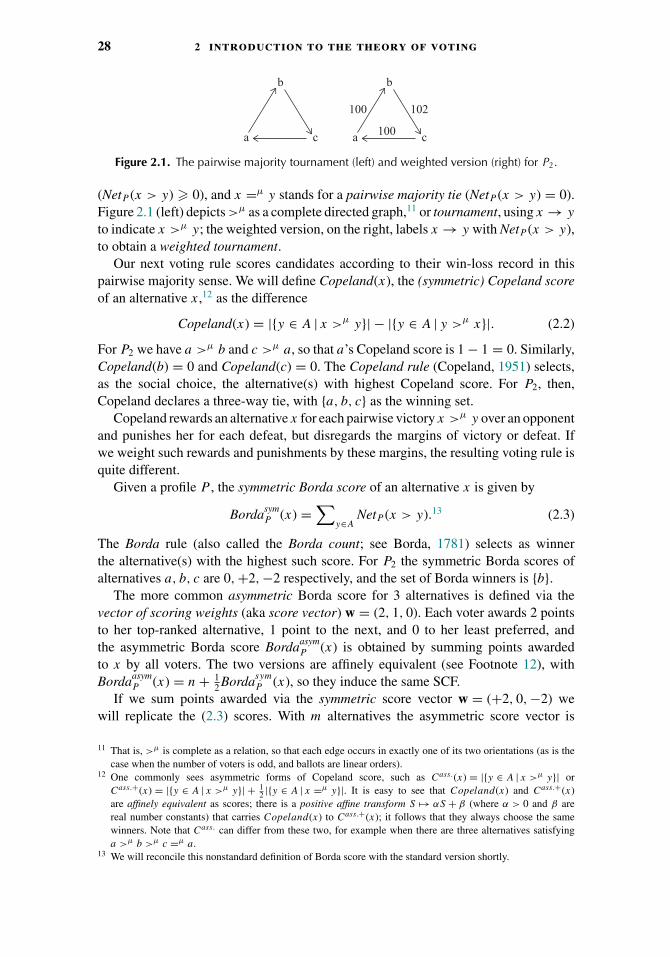
28 2 introduction to the theory of voting
a c
b
a
100 102
100 c
b
Figure 2.1. The pairwise majority tournament (left) and weighted version (right) for P2.
(NetP (x > y) � 0), and x =μ y stands for a pairwise majority tie (NetP (x > y) = 0).Figure 2.1 (left) depicts >μ as a complete directed graph,11 or tournament, using x → y
to indicate x >μ y; the weighted version, on the right, labels x → y with NetP (x > y),to obtain a weighted tournament.
Our next voting rule scores candidates according to their win-loss record in thispairwise majority sense. We will define Copeland(x), the (symmetric) Copeland scoreof an alternative x,12 as the difference
Copeland(x) = |{y ∈ A | x >μ y}| − |{y ∈ A | y >μ x}|. (2.2)
For P2 we have a >μ b and c >μ a, so that a’s Copeland score is 1 − 1 = 0. Similarly,Copeland(b) = 0 and Copeland(c) = 0. The Copeland rule (Copeland, 1951) selects,as the social choice, the alternative(s) with highest Copeland score. For P2, then,Copeland declares a three-way tie, with {a, b, c} as the winning set.
Copeland rewards an alternative x for each pairwise victory x >μ y over an opponentand punishes her for each defeat, but disregards the margins of victory or defeat. Ifwe weight such rewards and punishments by these margins, the resulting voting rule isquite different.
Given a profile P , the symmetric Borda score of an alternative x is given by
BordasymP (x) =
∑y∈A
NetP (x > y).13 (2.3)
The Borda rule (also called the Borda count; see Borda, 1781) selects as winnerthe alternative(s) with the highest such score. For P2 the symmetric Borda scores ofalternatives a, b, c are 0,+2,−2 respectively, and the set of Borda winners is {b}.
The more common asymmetric Borda score for 3 alternatives is defined via thevector of scoring weights (aka score vector) w = (2, 1, 0). Each voter awards 2 pointsto her top-ranked alternative, 1 point to the next, and 0 to her least preferred, andthe asymmetric Borda score Bordaasym
P (x) is obtained by summing points awardedto x by all voters. The two versions are affinely equivalent (see Footnote 12), withBordaasym
P (x) = n + 12 Bordasym
P (x), so they induce the same SCF.If we sum points awarded via the symmetric score vector w = (+2, 0,−2) we
will replicate the (2.3) scores. With m alternatives the asymmetric score vector is
11 That is, >μ is complete as a relation, so that each edge occurs in exactly one of its two orientations (as is thecase when the number of voters is odd, and ballots are linear orders).
12 One commonly sees asymmetric forms of Copeland score, such as Cass.(x) = |{y ∈ A | x >μ y}| orCass.+(x) = |{y ∈ A | x >μ y}| + 1
2 |{y ∈ A | x =μ y}|. It is easy to see that Copeland(x) and Cass.+(x)are affinely equivalent as scores; there is a positive affine transform S �→ αS + β (where α > 0 and β arereal number constants) that carries Copeland(x) to Cass.+(x); it follows that they always choose the samewinners. Note that Cass. can differ from these two, for example when there are three alternatives satisfyinga >μ b >μ c =μ a.
13 We will reconcile this nonstandard definition of Borda score with the standard version shortly.
2 .2 social choice functions: plurality, copeland, and borda 29
w = (m − 1, m − 2, m − 3, . . . , 0); the symmetric version w = (m − 1, m − 3, m −5, . . . ,−(m − 1)) replicates the scores from (2.3).14 An advantage of the symmet-ric approach embodied by (2.1), (2.2), and (2.3) is that it is well-defined for pro-files of weak preferences, yielding plausible extensions of the Borda and Copelandrules.15
As these examples suggest, our interest lies mainly with voting rules that take profilesof strict preferences as inputs, and return one alternative (the winner) or several (in theevent of a tie). Let C(X) denote the set of all nonempty subsets of a set X. Then:
Definition 2.1. A social choice function, or SCF, is a map f : L(A)n → C(A) thatreturns a nonempty set of alternatives for each profile of strict preferences. If |f (P )| = 1then f is single valued on P (and we sometimes write f (P ) = x instead of f (P ) ={x}). A resolute SCF is one with no ties: it is single valued on all profiles.16
We will also be interested in SCFs with restricted domain—voting rules that fit thedefinition, except that they are defined only on some proper subset of L(A)n. Definition2.1 associates each SCF with a single choice of N : these are fixed electorate SCFs;for variable electorate SCFs, substitute L(A)<∞ for L(A)n.17 The rest of this chapterpresumes a fixed electorate, except where explicitly noted otherwise.
Note that for the plurality, Copeland, and Borda SCFs the assignment of numericalscores does more than just select the socially most desirable alternative—it induces a“social ranking” in which one alternative is ranked over another when it has a higherscore. Tied scores are possible, so this is a “weak” ranking in R(A). Many social choicefunctions use mechanisms that yield a weak ranking of all alternatives, and so fit thefollowing definition:
Definition 2.2. A social welfare function, or SWF, is a map f : L(A)n → R(A)that returns a weak ranking of the set of alternatives for each profile of strictpreferences.18
A Taste of Strategic Manipulation
Do these rules give voters an incentive, on occasion, to cast insincere ballots? ConsiderAli, one of the two a � b � c � d � e voters of profile P3 (see later). Under Copeland,he is about to see his least preferred alternative win: e’s (symmetric) Copeland score is2, b’s is −2, and the other scores are each 0. If Ali misrepresents his sincere preferencesby completely reversing his ballot ranking, the Copeland winner shifts to d—which heprefers—with a score of 4, the maximum possible.
14 Any two scoring vectors of form w = (c, c − d, c − 2d, . . . , c − (m − 1)d), d > 0 have affinely equivalentscoring weights, yielding affinely equivalent total scores for the alternatives. Thus, the weak ordering ofalternatives induced by these scores is the same.
15 See last part of Section 2.10, including footnotes.16 Some authors reserve “SCF” for the resolute case, and use social choice correspondence (SCC) when multiple
winners are allowed.17 The fixed/variable distinction is often suppressed; Borda and Copeland fit both contexts, for example.18 Domains R(A)n and R(A)<∞ are also considered for SCFs and SWFs.

30 2 introduction to the theory of voting
2 3 2
e d ac e ba b cd c db a e
Definition 2.3. An SCF f is single voter manipulable if for some pair P , P ′ of profileson which f is single valued, and voter i with �′
j =�j for all j �= i, f (P ′) �i f (P );f is single voter strategyproof if it is not single voter manipulable.
We interpret �i (in Definition 2.3) as representing voter i’s sincere ranking; by switch-ing from �i to the insincere ballot �′
i voter i can change the winning alternative to onethat, according to her sincere ballot, she strictly prefers.
Notice that for each pair of alternatives, Ali’s reversed ballot of e � d � c � b � a
misrepresents which of the two he actually prefers. Under Borda, Ali alone can stillmanipulate profile P3, but not by completely reversing his ranking.19 Instead, by liftingd to the top (casting ballot d � a � b � c � e) Ali can get d to displace e, as earnerof the uniquely highest Borda score.
Plurality voting is not single voter manipulable; any one voter preferring y to theunique plurality winner x does not top-rank x on her sincere ballot, so she cannot lowerx’s score. At best she can raise y’s plurality score to a tie with x’s. However, if the twoe � c � a � b � d voters of P3 both switch to a � . . . the former plurality winner d
will be replaced by a, which they prefer. The example suggests that for rules with ties,single voter manipulability is an inappropriate test—we need to ban ties, or deal withthem, and we touch on both routes in Section 2.3.
2.3 Axioms I: Anonymity, Neutrality, and the Pareto Property
A variety of interesting SCFs have been proposed, often based on mechanisms thatseem to calculate the winner in an intuitively “fair” way. Experience suggests, however,that mechanisms may have unintended consequences that undercut their initial appeal.As a result, scholars have come to distrust arguments based solely on the intuitiveappeal of an underlying mechanism20 for calculating winners. They rely instead onaxioms—precisely defined properties of voting rules as functions (phrased withoutreferring to a particular mechanism). Axioms often have normative content, meaningthat they express, in some precise way, an intuitively appealing behavior we would likeour voting rules to satisfy (such as a form of fairness).
As applied to the theory of voting, the axiomatic method identifies interesting votingrules, formulates intuitively appealing or useful axioms, and proves theorems showingwhich rules satisfy which axioms. Ideally, such theorems characterize a class S of
19 The example thus shows that Copeland can be manipulated via complete reversal. Borda, on the other hand,can never be manipulated in this way—see later discussion of half-way monotonicity in Section 2.6.
20 As we already glimpsed in the case of the Borda SCF, a function may be computable via a variety of mechanisms,not all having the same intuitive appeal. Which of them should determine the intuitive appeal of the commonfunction they compute? This is a second reason to be cautious when passing judgment as to the fairness of avoting rule based on its mechanism alone.
2 .3 axioms i: anonymity, neutrality, and the pareto property 31
voting rules via a set A of axioms, by proving that S contains exactly those rulessatisfying all axioms in A. Such theorems may uniquely characterize one rule in termsof its properties (when S is a singleton), or demonstrate the impossibility of satisfyingall properties of A (by showing S to be empty). In fact, impossibilities are among themost consequential results in the field, for it turns out that axioms also have unintendedconsequences . . . as when one seemingly reasonable axiom rules out any hope ofsatisfying some other one.
Axioms for SCFs can be loosely sorted into three groups. The first group representminimal demands. These axioms are absolutely required (for some contexts) and plentyof SCFs satisfy them (including plurality, Borda, and Copeland). There is little cost,then, to requiring them and they seem, as well, to offer less scope for unintendedconsequences, so they tend to be seen as uncontroversial.
In this section we discuss five axioms from the first group. In Section 2.6 we considera second group of axioms, of middling strength—they are satisfied by some interestingSCFs, but requiring any one of these axioms would have a high cost: some veryattractive rules, and some of the other axioms from the same group, would be ruled out.These axioms are the most controversial; your favorite voting rule may violate someaxiom from this group, and be seen as illegitimate by anyone who finds that axiom tobe compelling. A third group of axioms include strategyproofness and IIA, and theseare the strongest, in that they tend to rule out all reasonable voting rules. Of coursethese axioms are associated with some controversy, in terms of how one interprets thecorresponding impossibilities—does Arrow’s Theorem really say that democracy isimpossible? Or does a closer look at IIA suggest that it is less compelling than mightfirst appear? But there is no controversy over whether or not to impose any of theseaxioms when choosing an SCF—the cost is too high.21
Definition 2.4. An SCF f is anonymous if each pair of voters play interchangeableroles: f (P ) = f (P �) holds whenever a profile P � is obtained from another P byswapping the ballots cast by some two voters i and j (��
i=�j , ��j=�i , and ��
k=�k
for all k �= i, j );22 f is dictatorial if some voter i acts as dictator, meaning f (P )coincides with i’s top-ranked alternative, for every profile P .
Anonymity is a very strong form of equal treatment of voters, and nondictatorialityserves as a particularly weak version of anonymity.
Definition 2.5. An SCF f is neutral if each pair of alternatives are interchangeable inthe following sense: whenever a profile P † is obtained from another P by swapping thepositions of the two alternatives x and y in every ballot, the outcome f (P †) is obtained
21 We should qualify, in at least two respects, the picture painted here. First, there are important strands of researchthat are not axiomatic—they do not measure the success or failure of some SCF to satisfy some property inblack-or-white terms. These include empirical and experimental methods in the political realm (e.g., van derStraeten et al., 2013), as well as enumerations and simulations (e.g., Kelly, 1993; Aleskerov and Kurbanov,1999). Second, while strategyproofness may be impractical as a requirement for SCFs, it can be achieved insome collective decision-making contexts other than voting (Moulin, 1988a). Moreover, SCFs can achievestrategyproofness when their domains are limited appropriately, as we see in Section 2.9.
22 Transpositions τij of pairs generate the full permutation group on N , so anonymity demands that f be blindto every permutation of the voters; informally, “f is invariant under renaming voters.” Anonymous SCFs arethose that use only the information in the voting situation derived from a profile P (which represents P ’sequivalence class under permutations of voters).
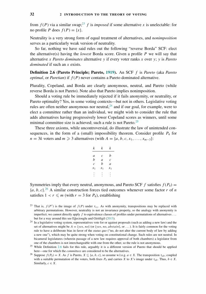
32 2 introduction to the theory of voting
from f (P ) via a similar swap;23 f is imposed if some alternative x is unelectable: forno profile P does f (P ) = {x}.Neutrality is a very strong form of equal treatment of alternatives, and nonimpositionserves as a particularly weak version of neutrality.
So far, nothing we have said rules out the following “reverse Borda” SCF: electthe alternative(s) having the lowest Borda score. Given a profile P we will say thatalternative x Pareto dominates alternative y if every voter ranks x over y; y is Paretodominated if such an x exists.
Definition 2.6 (Pareto Principle; Pareto, 1919). An SCF f is Pareto (aka Paretooptimal, or Paretian) if f (P ) never contains a Pareto dominated alternative.
Plurality, Copeland, and Borda are clearly anonymous, neutral, and Pareto (whilereverse Borda is not Pareto). Note also that Pareto implies nonimposition.
Should a voting rule be immediately rejected if it fails anonymity, or neutrality, orPareto optimality? Yes, in some voting contexts—but not in others. Legislative votingrules are often neither anonymous nor neutral,24 and if our goal, for example, were toelect a committee rather than an individual, we might wish to consider the rule thatadds alternatives having progressively lower Copeland scores as winners, until someminimal committee size is achieved; such a rule is not Pareto.25
These three axioms, while uncontroversial, do illustrate the law of unintended con-sequences, in the form of a (small) impossibility theorem. Consider profile P4 forn = 3k voters and m � 3 alternatives (with A = {a, b, c, x1, . . . , xm−3}:
k k k
a c bb a cc b ax1 x1 x1
......
...
Symmetries imply that every neutral, anonymous, and Pareto SCF f satisfies f (P4) ={a, b, c}.26 A similar construction forces tied outcomes whenever some factor r of n
satisfies 1 < r � m (with r = 3 for P4), establishing
23 That is, f (P †) is the image of f (P ) under τxy . As with anonymity, transpositions may be replaced witharbitrary permutations. However, neutrality is not an invariance property, so the analogy with anonymity isimperfect; we cannot directly apply f to equivalence classes of profiles under permutations of alternatives . . .but for a way around this see Egeciouglu and Giritligil (2013).
24 In a legislative voting system, representatives vote for or against proposals (such as adding a new law) and theset of alternatives might be A = {yes, no} (or {yes, no, abstain}, or . . . ). It is fairly common for the votingrule to have a deliberate bias in favor of the status quo (“no, do not alter the current body of law by addinga new one”), which may be quite strong when voting on constitutional change. Such rules are not neutral. Inbicameral legislatures (wherein passage of a new law requires approval of both chambers) a legislator fromone of the chambers is not interchangeable with one from the other, so the rule is not anonymous.
25 While Definition 2.6 fails for this rule, arguably it is a different version of Pareto that should be appliedhere—one for which the committees are considered to be the alternatives.
26 Suppose f (P4) = X. As f is Pareto, X ⊆ {a, b, c}, so assume w.l.o.g. a ∈ X. The transposition τab , coupledwith a suitable permutation of the voters, both fixes P4 and carries X to X’s image under τab . Thus, b ∈ X.Similarly, c ∈ X.
2 .4 voting rules i 33
Proposition 2.1 (Moulin, 1983). Let m � 2 be the number of alternatives and n bethe number of voters. If n is divisible by any integer r with 1 < r � m, then no neutral,anonymous, and Pareto SCF is resolute (single-valued).27
Tied outcomes make life complicated in terms of real applications (we only wantone mayor) and of theory: how can we decide whether a strategically cast ballot resultsin a successful manipulation, if both it and the sincere ballot yield several winningalternatives? The four main approaches taken in the literature28 are as follows:
1. Use a fixed ordering of the alternatives (or a designated voter) to break all ties.2. Use a randomized mechanism to break all ties.3. Deal with set-valued outcomes directly.4. Ignore or suppress the issue (assume no ties exist).
The first approach breaks neutrality (or anonymity, if using a designated voter).The second requires that we consider “indeterminate” voting rules, along with what itmeans to manipulate one. With approach 3, adapting the definitions (in Section 2.6) ofmonotonicity properties and strategyproofness might seem to require choosing a “setextension principle” (which extends preferences over individual alternatives to onesover sets), although alternative approaches exist.29
We can agree that approach 4 is quite reasonable as a preliminary, simplifyingassumption when first exploring some new concept. As to the importance of (or interestin) a subsequent careful reconsideration of that concept in light of ties, opinions differ.
2.4 Voting Rules I: Condorcet Extensions, Scoring Rules,and Run-Offs
When there are only two alternatives, the distinction between a preference ranking anda plurality ballot disappears, and one SCF in particular jumps to mind. Majority ruledeclares the winner to be the alternative that gets strictly more votes, with a two-waytie when the alternatives split the vote evenly. Majority rule is neutral and anonymous,and is resolute if the number of voters is odd. A characterization, however, requires anadditional element of monotonicity (if x is a winner and one voter switches her ballotfrom y to x, then x remains a winner) or of positive responsiveness (if x is a winnerand one voter switches her ballot from y to x, then x becomes the unique winner).Monotonicity excludes certain perverse rules (e.g., elect whichever alternative gets anodd number of votes) while positive responsiveness additionally breaks all ties that are
27 If every factor of n exceeds m, then a resolute SCF can be neutral, anonymous, and Pareto. See later discussionimmediately after Theorem 2.7.
28 For a fifth approach, see Footnote 66. In real world political elections with large numbers of voters, electionreturns may be too “noisy” to declare an exact tie with certainty, and very close elections are sometimes settledin court. However, some countries have election laws that mandate coin tosses to settle ties; in 2013 the mayoralelection in San Teodoro, the Philipines, was settled this way. The French electoral code specifies that ties bebroken in favor of the older candidate (consequently, parties favor older candidates in some elections).
29 For more on these approaches—which are less different than may first appear—see Gardenfors (1976),Gardenfors (1979), Barbera et al. (2001), Barbera et al. (2004), Brandt and Brill (2011), Sanver and Zwicker(2012).

34 2 introduction to the theory of voting
not “knife-edge” (excluding, for example, the rule electing all alternatives getting atleast one third of the vote).
Proposition 2.2 (May’s Theorem; May, 1952). For two alternatives and an oddnumber of voters, majority rule is the unique resolute, anonymous, neutral, and mono-tonic SCF. For two alternatives and any number of voters, it is the unique anonymous,neutral, and positively responsive SCF.
Proof. It is evident that majority rule satisfies these properties. For uniqueness, notethat with any other rule we may choose a profile for which x wins with fewer votes thany. Switch enough ballots from y to x to exactly reverse these vote totals. Monotonicityimplies x still wins, but neutrality + anonymity say y wins. Similarly, if x ties y, yethas fewer votes, positive responsiveness contradicts neutrality + anonymity.
It is not unreasonable to interpret Proposition 2.2 as saying that majority rule is thebest voting rule for two alternatives (in certain contexts, anyway). So, which SCFs canclaim the mantle as “majority rule for 3 or more alternatives”? On one hand, each ofthe SCFs we have considered so far (along with a host of others) reduces to majorityrule for the case m = 2, and in quite a natural way. So one might argue that most rulescan claim this mantle. On the other hand, for SCFs defined on the “full domain” (allof L(A)n) there is no completely satisfactory extension of May’s Theorem to the caseof 3 or more alternatives.30 In this sense, then, no voting method wins the mantle.Nonetheless, one rule has long claimed a special place as most deserving:
Definition 2.7. A Condorcet winner for a profile P is an alternative x that defeatsevery other alternative in the strict pairwise majority sense: x >
μP y for all y �= x.31
Pairwise Majority Rule, henceforth PMR, declares the winning alternative to be theCondorcet winner . . . and is undefined when a profile has no Condorcet winner.
When a Condorcet winner exists, it is unique. With three or more alternatives,however, majority cycles can rule them out. The cycle a >μ b, b >μ c, and c >μ a
of profile P2 is depicted in Figure 2.1; no PMR winner exists. Such a cycle is alsoknown as Condorcet’s voting paradox, and corresponds to intransitivity of the relation>μ. Cycles represent a disturbing type of instability. Imagine a version with 10 votersand 10 alternatives,32 wherein any alternative x selected as winner would prompt 90%of the voters to agree on an alternative y they all prefer to x and to approve, by anoverwhelming margin, a referendum replacing x with y. A different 90% would thenreplace y with z, and so on. One cannot overstate the importance of majority cycles tothe theory of voting—they lie behind a number of the most important results.
A significant literature is concerned with calculating the probability that a Condorcetwinner exists (or that �μ is transitive), or the Condorcet efficiency of a voting rule—theconditional probability that the rule elects the Condorcet winner, given that a Condorcet
30 Such extensions do exist in voting contexts other than SCFs (see Freixas and Zwicker (2009), for example)and also for SCFs on restricted domains (as we will see in a moment).
31 Some prefer strong Condorcet winner for this notion; a weak Condorcet winner satisfies x �μP y for all y �= x.
32 Voter 1 ranks a on top, with b through j following in alphabetical order; each subsequent ballot is derivedfrom its predecessor by “vertical rotation”: lift the bottom-ranked alternative to the top, and drop each of theothers down by one spot.
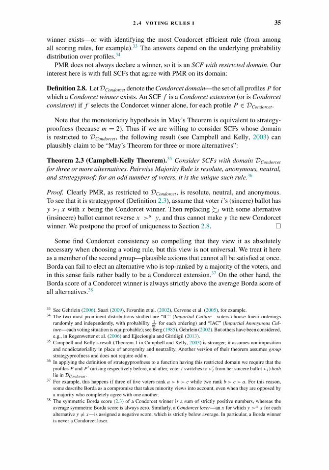
2 .4 voting rules i 35
winner exists—or with identifying the most Condorcet efficient rule (from amongall scoring rules, for example).33 The answers depend on the underlying probabilitydistribution over profiles.34
PMR does not always declare a winner, so it is an SCF with restricted domain. Ourinterest here is with full SCFs that agree with PMR on its domain:
Definition 2.8. LetDCondorcet denote the Condorcet domain—the set of all profiles P forwhich a Condorcet winner exists. An SCF f is a Condorcet extension (or is Condorcetconsistent) if f selects the Condorcet winner alone, for each profile P ∈ DCondorcet.
Note that the monotonicity hypothesis in May’s Theorem is equivalent to strategy-proofness (because m = 2). Thus if we are willing to consider SCFs whose domainis restricted to DCondorcet, the following result (see Campbell and Kelly, 2003) canplausibly claim to be “May’s Theorem for three or more alternatives”:
Theorem 2.3 (Campbell-Kelly Theorem).35 Consider SCFs with domain DCondorcet
for three or more alternatives. Pairwise Majority Rule is resolute, anonymous, neutral,and strategyproof; for an odd number of voters, it is the unique such rule.36
Proof. Clearly PMR, as restricted to DCondorcet, is resolute, neutral, and anonymous.To see that it is strategyproof (Definition 2.3), assume that voter i’s (sincere) ballot hasy �i x with x being the Condorcet winner. Then replacing �i with some alternative(insincere) ballot cannot reverse x >μ y, and thus cannot make y the new Condorcetwinner. We postpone the proof of uniqueness to Section 2.8.
Some find Condorcet consistency so compelling that they view it as absolutelynecessary when choosing a voting rule, but this view is not universal. We treat it hereas a member of the second group—plausible axioms that cannot all be satisfied at once.Borda can fail to elect an alternative who is top-ranked by a majority of the voters, andin this sense fails rather badly to be a Condorcet extension.37 On the other hand, theBorda score of a Condorcet winner is always strictly above the average Borda score ofall alternatives.38
33 See Gehrlein (2006), Saari (2009), Favardin et al. (2002), Cervone et al. (2005), for example.34 The two most prominent distributions studied are “IC” (Impartial Culture—voters choose linear orderings
randomly and independently, with probability 1m! for each ordering) and “IAC” (Impartial Anonymous Cul-
ture—each voting situation is equiprobable); see Berg (1985), Gehrlein (2002). But others have been considered,e.g., in Regenwetter et al. (2006) and Egeciouglu and Giritligil (2013).
35 Campbell and Kelly’s result (Theorem 1 in Campbell and Kelly, 2003) is stronger; it assumes nonimpositionand nondictatoriality in place of anonymity and neutrality. Another version of their theorem assumes groupstrategyproofness and does not require odd n.
36 In applying the definition of strategyproofness to a function having this restricted domain we require that theprofiles P and P ′ (arising respectively before, and after, voter i switches to �′
i from her sincere ballot �i ) bothlie in DCondorcet .
37 For example, this happens if three of five voters rank a � b � c while two rank b � c � a. For this reason,some describe Borda as a compromise that takes minority views into account, even when they are opposed bya majority who completely agree with one another.
38 The symmetric Borda score (2.3) of a Condorcet winner is a sum of strictly positive numbers, whereas theaverage symmetric Borda score is always zero. Similarly, a Condorcet loser—an x for which y >μ x for eachalternative y �= x—is assigned a negative score, which is strictly below average. In particular, a Borda winneris never a Condorcet loser.
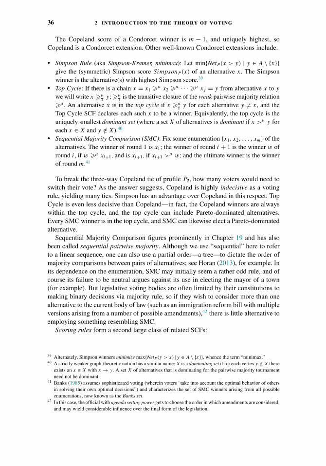
36 2 introduction to the theory of voting
The Copeland score of a Condorcet winner is m − 1, and uniquely highest, soCopeland is a Condorcet extension. Other well-known Condorcet extensions include:
� Simpson Rule (aka Simpson-Kramer, minimax): Let min{NetP (x > y) | y ∈ A \ {x}}give the (symmetric) Simpson score SimpsonP (x) of an alternative x. The Simpsonwinner is the alternative(s) with highest Simpson score.39
� Top Cycle: If there is a chain x = x1 �μ x2 �μ · · · �μ xj = y from alternative x to y
we will write x �μᵀ y; �μ
ᵀ is the transitive closure of the weak pairwise majority relation�μ. An alternative x is in the top cycle if x �μ
ᵀ y for each alternative y �= x, and theTop Cycle SCF declares each such x to be a winner. Equivalently, the top cycle is theuniquely smallest dominant set (where a set X of alternatives is dominant if x >μ y foreach x ∈ X and y /∈ X).40
� Sequential Majority Comparison (SMC): Fix some enumeration {x1, x2, . . . , xm} of thealternatives. The winner of round 1 is x1; the winner of round i + 1 is the winner w ofround i, if w �μ xi+1, and is xi+1, if xi+1 >μ w; and the ultimate winner is the winnerof round m.41
To break the three-way Copeland tie of profile P2, how many voters would need toswitch their vote? As the answer suggests, Copeland is highly indecisive as a votingrule, yielding many ties. Simpson has an advantage over Copeland in this respect. TopCycle is even less decisive than Copeland—in fact, the Copeland winners are alwayswithin the top cycle, and the top cycle can include Pareto-dominated alternatives.Every SMC winner is in the top cycle, and SMC can likewise elect a Pareto-dominatedalternative.
Sequential Majority Comparison figures prominently in Chapter 19 and has alsobeen called sequential pairwise majority. Although we use “sequential” here to referto a linear sequence, one can also use a partial order—a tree—to dictate the order ofmajority comparisons between pairs of alternatives; see Horan (2013), for example. Inits dependence on the enumeration, SMC may initially seem a rather odd rule, and ofcourse its failure to be neutral argues against its use in electing the mayor of a town(for example). But legislative voting bodies are often limited by their constitutions tomaking binary decisions via majority rule, so if they wish to consider more than onealternative to the current body of law (such as an immigration reform bill with multipleversions arising from a number of possible amendments),42 there is little alternative toemploying something resembling SMC.
Scoring rules form a second large class of related SCFs:
39 Alternately, Simpson winners minimize max{NetP (y > x) | y ∈ A \ {x}}, whence the term “minimax.”40 A strictly weaker graph-theoretic notion has a similar name: X is a dominating set if for each vertex y /∈ X there
exists an x ∈ X with x → y. A set X of alternatives that is dominating for the pairwise majority tournamentneed not be dominant.
41 Banks (1985) assumes sophisticated voting (wherein voters “take into account the optimal behavior of othersin solving their own optimal decisions”) and characterizes the set of SMC winners arising from all possibleenumerations, now known as the Banks set.
42 In this case, the official with agenda setting power gets to choose the order in which amendments are considered,and may wield considerable influence over the final form of the legislation.

2 .4 voting rules i 37
Definition 2.9. A score vector w = (w1, w2, . . . , wm) consists of real number scoringweights; w is proper if w1 � w2 � · · · � wm−1 � wm and w1 > wm. Any score vectorinduces a scoring rule, in which each voter awards w1 points to their top-rankedalternative, w2 points to their second-ranked, and so on. All points awarded to a givenalternative are summed, and the winner is the alternative(s) with greatest sum.43 Aproper scoring rule is one induced by a proper score vector.
In addition to the Borda count, with w = (m − 1, m − 2, . . . , 1, 0), scoring rulesinclude:
� Plurality: w = (1, 0, 0, . . . , 0)� Anti-plurality: w = (1, 1, 1, . . . , 1, 0)� k-Approval: w = (1, 1, 1, . . . , 1, 0, 0, . . . , 0) (with k 1s)� Formula One Championship: w = (25, 18, 15, 12, 10, 8, 6, 4, 2, 1, 0, . . . , 0)44
A third class of multiround rules is based on the idea that less popular alternatives inone round be dropped from all ballots in the next round (with each ballot then rankingthe remaining alternatives in the same relative order that they had in the initial version ofthat ballot); these rounds continue until some surviving alternative achieves majoritysupport (or until only one is left standing). The best-known of these has multiplenames—Alternative Vote, Hare (Hare, 1859), Single Transferable Vote (STV), InstantRun-off Voting (IRV), and Ranked Choice Voting (RCV)—and proceeds as follows: ateach stage, the alternative with lowest plurality score is dropped from all ballots, andat the first stage for which some alternative x sits atop a majority of the ballots, x isdeclared the winner.45
Related rules include the following:
� Plurality Run-off : If some alternative is top ranked by a majority of the voters, it winsin round 1; otherwise, round 2 consists of majority rule applied to the two alternativeswith highest plurality score in round 1.
� Baldwin: In each round, the alternative with lowest Borda score is dropped. The finalalternative eliminated is the winner (Baldwin, 1926).
� Nanson: In each round, drop all alternatives with below-average Borda score. The finalalternative eliminated is the winner (Nanson, 1882; Niou, 1987).
43 Alternately a SWF can be defined by ranking alternatives in descending order of point totals.44 Since 2010, a driver gets 25 points for each Formula One Grand Prix race they win, 18 points for each second
place, etc., and the World Championship goes to the driver with greatest point total for that season. In effect,the races serve as voters. Related rules have been used since 1950, but in some earlier versions a driver wasawarded points for his or her top j finishes only.
45 The vexing matter of how to deal with ties for lowest plurality score is often ignored, perhaps because for large,political elections uncertainties in counting (and in classifying ballots as valid or not) leave the matter moot.One method suggested (Taylor and Pacelli, 2006) is to drop all alternatives sharing a lowest plurality score. Ifeach of k � 3 surviving alternatives garners the same plurality score, this method eliminates all of them, withno alternative ever achieving majority support (unless one eliminates the stop-when-there-is-a-majority ruleand instead declares, as winners, all alternatives eliminated in the final round). The second (Conitzer et al.,2009b) chooses at each stage one alternative to eliminate, among those achieving minimal plurality score, butconsiders all possible sequences of such choices, identifying the winning alternative for each sequence, anddeclaring a tie among them.

38 2 introduction to the theory of voting
STV is perhaps the most popular rule among electoral reform societies.46 Supportersargue that voters do not “waste” their vote when their top choice is unpopular—instead,it is transferred to the next choice on their ballot. Plurality run-off is a bit differentin being limited to two rounds at most, but agrees with STV for three alternatives.Neither of these systems is a Condorcet extension.47,48 Both Baldwin and Nanson areCondorcet extensions, as the elimination process never discards a Condorcet winner; forthe explanation see Footnote 38, which also shows that Nanson discards any Condorcetloser in round one.
2.5 An Informational Basis for Voting Rules: Fishburn’sClassification
Figure 2.1 (left) depicts the pairwise majority tournament for profile P2—the completedirected graph induced by >μ (see Footnote 11). To calculate a winner, the Copeland,Top Cycle, and Sequential Majority Comparison SCFs need only the information fromthis tournament. Peter Fishburn (1977) classified such SCFs as C1 functions; looselyspeaking, such SCFs correspond to tournament solutions as studied in Chapter 3.49
Borda and Simpson need the additional information in the weighted tournament—the net preferences50 of Figure 2.1 (right)—and are classified in C2. Imagine that eachvoter’s ranking �i is represented as a set of ordered pairs in the usual way, and a union(counting multiplicity) of all rankings from the profile is taken. Ordered pairs in thismultiset are sorted into bins according to which two alternatives are in the pair. ThenC2 functions rely only on the information represented by these bins; what is lost is
46 In the United Kingdom a 2011 referendum proposing a switch from plurality voting to STV lost when almost68% voted No. In the United States the FairVote organization advocates STV (under the IRV name), andhas been successful in some locales. For example, the city of Burlington, Vermont, adopted IRV for its 2006mayoral election and later repealed it, when in 2009 the IRV winner (Kiss) differed from the plurality winner(Wright). One analysis argued that the Condorcet winner was a third candidate (Montroll), and that the “noshow” paradox (discussed after Proposition 2.6) had applied. See http://rangevoting.org/Burlington.html andhttp://vermontdailybriefing.com/?p=1215.
47 Consider any profile for 4 alternatives wherein alternative a is ranked second by all voters, with each of theother alternatives ranked first by around one third of the voters. The Condorcet winner a is eliminated in thefirst round.
48 A version of plurality run-off is used for presidential elections in France, Austria , . . . indeed, in more countriesthan use plurality (see Blais et al., 1997); voters do not submit ranked ballots, but instead return to the ballotbox if a second round is required. The method attracted international attention in the 2002 French election,when the far-right candidate Le Pen bested the Socialist Jospin in round one, and ran against the incumbentChirac in round two (which Chirac won with over 82% of the vote, after having captured under 20% in roundone). Reportedly, voters with allegiance to small left-wing parties chose to vote for these parties in roundone, assuming that Jospin would survive to round two, when they would vote for him. In round one of the2012 election Francois Bayrou came in fifth, with 11% of the vote, yet data suggests that he may have been aCondorcet winner (van der Straeten et al., 2013); there is some uncertainty because the conclusion is sensitiveto the method used to control sample bias (private communication of the authors).
49 Unlike an SCF, a tournament solution takes as input only the tournament itself (rather than an underlyingprofile that may have induced that tournament). Also, a tournament solution f is often assumed to satisfy theconditions corresponding to neutrality and Condorcet extension (for the C1 SCF f � induced by f ).
50 Alternately, for each two alternatives draw edges in both directions, labeling the x → y edge with grosspreference (absolute number of voters ranking x over y). In a fixed electorate context one knows the numbern of voters, so the information in these labels is equivalent to the net preferences.

2 .6 axioms ii: reinforcement and monotonicity properties 39
a
b
d
c01 1
10 0
a
b
d
c00 –1
10 1
Figure 2.2. A basic cocycle (left) and a basic cycle (right). The −1 on edge d → c indicatesthat its pre-assigned orientation opposes the cycle’s clockwise direction.
whether a given (a, b) pair came from a ranking with (b, c) or one with (c, b). Socialchoice functions in C2 correspond (speaking as loosely as in the previous paragraph)to weighted tournament solutions—the topic of Chapter 4.
Any SCFs not in C1 or C2 are C3. In a sense, C3 SCFs need “more” information;the bins of atomized pairs are insufficient. But plurality is in C3, and one should balkat a suggestion that Borda needs less information than plurality. Borda, for example,needs all the information in the rank vector ρ(x) = (ρ1(x), ρ2(x), . . . , ρm(x)) of analternative x (where ρj (x) denotes the number of voters who rank x in j th position),while plurality does not. Thus while Fishburn’s classification is a particularly usefulapproach to informational bases, it is not the only such approach.
A further refinement of C2 is based on the orthogonal decomposition approaches ofZwicker (1991) and Saari (1995). Any weighted tournament can be viewed as a vector vwhose scalar components are the edge weights. As such, v has a unique decompositionv = vcycle + vcocycle with vcycle ⊥ vcocycle, wherein vcycle is a linear combination of basiccycles and vcocycle is a linear combination of basic cocycles—see Figure 2.2 (for thecase of 4 alternatives).
We may interpret vcycle as the underlying tendency toward a majority cycle, whilevcocycle contains exactly the same information as the list of symmetric Borda scores.51,52
Condorcet extensions use the information in both components, while the Borda countdiscards vcycle and imposes a version of pairwise majority rule based on vcocycle alone.53
Whether the ranking according to PMR (the true version, based on both components)agrees with the ranking induced by Borda score, or differs from it, or fails to be aranking at all, depends on the relative balance (speaking loosely) between vcocycle andvcycle.
2.6 Axioms II: Reinforcement and Monotonicity Properties
We consider axioms that distinguish among the three classes of rules introduced in theprevious section. More than two hundred years ago Condorcet and Borda disagreed
51 This same decomposition serves as a basis for Kirchoff’s laws, where the edge weights represent flow ofelectric current (rather than flow of net preference, as in our setting); a basic cocycle is a sink or source ofcurrent (such as a battery) while a simple cycle is a “loop current.”
52 The asymmetric scores encode one additional piece of information: the number of voters.53 The map that discards vcycle is an orthogonal projection, and coincides with the boundary map of homology
theory in the one-dimensional case. The version of PMR based on vcocycle alone satisfies a strong, quantitativetransitivity property.
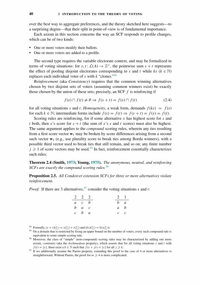
40 2 introduction to the theory of voting
over the best way to aggregate preferences, and the theory sketched here suggests—toa surprising degree—that their split in point-of-view is of fundamental importance.
Each axiom in this section concerns the way an SCF responds to profile changes,which can be of two kinds:
� One or more voters modify their ballots.� One or more voters are added to a profile.
The second type requires the variable electorate context, and may be formalized interms of voting situations: for s, t : L(A) → Z+, the pointwise sum s + t representsthe effect of pooling disjoint electorates corresponding to s and t while ks (k ∈ N)replaces each individual voter of s with k “clones.”54
Reinforcement (aka Consistency) requires that the common winning alternativeschosen by two disjoint sets of voters (assuming common winners exist) be exactlythose chosen by the union of these sets; precisely, an SCF f is reinforcing if
f (s) ∩ f (t) �= ∅ ⇒ f (s + t) = f (s) ∩ f (t) (2.4)
for all voting situations s and t . Homogeneity, a weak form, demands f (ks) = f (s)for each k ∈ N; intermediate forms include f (s) = f (t) ⇒ f (s + t) = f (s) = f (t).
Scoring rules are reinforcing, for if some alternative x has highest score for s andt both, then x’s score for s + t (the sum of x’s s and t scores) must also be highest.The same argument applies to the compound scoring rules, wherein any ties resultingfrom a first score vector w1 may be broken by score differences arising from a secondsuch vector w2 (e.g., use plurality score to break ties among Borda winners), with apossible third vector used to break ties that still remain, and so on; any finite numberj � 1 of score vectors may be used.55 In fact, reinforcement essentially characterizessuch rules:
Theorem 2.4 (Smith, 1973; Young, 1975). The anonymous, neutral, and reinforcingSCFs are exactly the compound scoring rules.56
Proposition 2.5. All Condorcet extension SCFs for three or more alternatives violatereinforcement.
Proof. If there are 3 alternatives,57 consider the voting situations s and t :
2 2 2a c b
b a c
c b a
2 1b a
a b
c c
54 Formally, (s + t)(�) = s(�) + t(�) and (ks)(�) = k(s(�)).55 On a domain that is restricted by fixing an upper bound on the number of voters, every such compound rule is
equivalent to some simple scoring rule.56 Moreover, the class of “simple” (non-compound) scoring rules may be characterized by adding one more
axiom, continuity (aka the Archimedean property), which asserts that for all voting situations s and t withf (t) = {x}, there exist a k ∈ N such that f (s + j t) = {x} for all j � k.
57 If we additionally assume the Pareto property, extending this proof to the case of 4 or more alternatives isstraightforward. Without Pareto, the proof for m � 4 is more complicated.
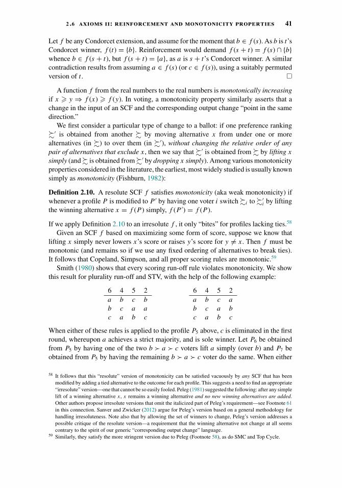
2 .6 axioms ii: reinforcement and monotonicity properties 41
Let f be any Condorcet extension, and assume for the moment that b ∈ f (s). As b is t’sCondorcet winner, f (t) = {b}. Reinforcement would demand f (s + t) = f (s) ∩ {b}whence b ∈ f (s + t), but f (s + t) = {a}, as a is s + t’s Condorcet winner. A similarcontradiction results from assuming a ∈ f (s) (or c ∈ f (s)), using a suitably permutedversion of t .
A function f from the real numbers to the real numbers is monotonically increasingif x � y ⇒ f (x) � f (y). In voting, a monotonicity property similarly asserts that achange in the input of an SCF and the corresponding output change “point in the samedirection.”
We first consider a particular type of change to a ballot: if one preference ranking�′ is obtained from another � by moving alternative x from under one or morealternatives (in �) to over them (in �′), without changing the relative order of anypair of alternatives that exclude x, then we say that �′ is obtained from � by lifting x
simply (and� is obtained from�′ by dropping x simply). Among various monotonicityproperties considered in the literature, the earliest, most widely studied is usually knownsimply as monotonicity (Fishburn, 1982):
Definition 2.10. A resolute SCF f satisfies monotonicity (aka weak monotonicity) ifwhenever a profile P is modified to P ′ by having one voter i switch �i to �′
i by liftingthe winning alternative x = f (P ) simply, f (P ′) = f (P ).
If we apply Definition 2.10 to an irresolute f , it only “bites” for profiles lacking ties.58
Given an SCF f based on maximizing some form of score, suppose we know thatlifting x simply never lowers x’s score or raises y’s score for y �= x. Then f must bemonotonic (and remains so if we use any fixed ordering of alternatives to break ties).It follows that Copeland, Simpson, and all proper scoring rules are monotonic.59
Smith (1980) shows that every scoring run-off rule violates monotonicity. We showthis result for plurality run-off and STV, with the help of the following example:
6 4 5 2a b c b
b c a a
c a b c
6 4 5 2a b c a
b c a b
c a b c
When either of these rules is applied to the profile P5 above, c is eliminated in the firstround, whereupon a achieves a strict majority, and is sole winner. Let P6 be obtainedfrom P5 by having one of the two b � a � c voters lift a simply (over b) and P7 beobtained from P5 by having the remaining b � a � c voter do the same. When either
58 It follows that this “resolute” version of monotonicity can be satisfied vacuously by any SCF that has beenmodified by adding a tied alternative to the outcome for each profile. This suggests a need to find an appropriate“irresolute” version—one that cannot be so easily fooled. Peleg (1981) suggested the following: after any simplelift of a winning alternative x, x remains a winning alternative and no new winning alternatives are added.Other authors propose irresolute versions that omit the italicized part of Peleg’s requirement—see Footnote 61in this connection. Sanver and Zwicker (2012) argue for Peleg’s version based on a general methodology forhandling irresoluteness. Note also that by allowing the set of winners to change, Peleg’s version addresses apossible critique of the resolute version—a requirement that the winning alternative not change at all seemscontrary to the spirit of our generic “corresponding output change” language.
59 Similarly, they satisfy the more stringent version due to Peleg (Footnote 58), as do SMC and Top Cycle.

42 2 introduction to the theory of voting
procedure is now run on P7, alternative b is eliminated first, whereupon c displaces a
as the new majority winner, with 9 of the 17 ballots.If we used an alternative definition of monotonicity allowing several voters to
simultaneously lift the winning alternative, then monotonicity would fail as P5 �→ P7
(in one step). For our version we observe that no matter what set X of winners results60
from P6, there must be a failure of monotonicity in the first step {a} �→ X (as P5 �→ P6)or in the second X �→ {c} (as P6 �→ P7).61
Now suppose the last two voters of P7 truly prefer a � b � c. They will be disap-pointed under STV when the winner turns out to be c. They would do better by castingb � a � c, and achieving a win for their most preferred alternative a. Indeed, anyfailure of monotonicity for a resolute SCF f represents an opportunity for a voter tomanipulate f in a particular way: via a simple drop or simple lift.62 Thus monotonicityis a weak form of strategyproofness. The same holds for the following monotonicityproperties (except for participation):
Definition 2.11. A resolute SCF f satisfies:
� Strategyproofness if whenever a profile P is modified to P ′ by having one voter i switch�i to �′
i , f (P ) �i f (P ′).63
� Maskin monotonicity (aka strong monotonicity) if whenever a profile P is modified toP ′ by having one voter i switch �i to a ballot �′
i satisfying for all y f (P ) �i y ⇒f (P ) �′
i y, f (P ′) = f (P ); see Maskin (1977), Maskin (1999).� Down monotonicity if whenever a profile P is modified to P ′ by having one voter i
switch �i to �′i by dropping a losing alternative b �= f (P ) simply, f (P ′) = f (P ).
� One-way monotonicity if whenever a profile P is modified to P ′ by having one voter i
switch �i to �′i , f (P ) �i f (P ′) or f (P ′) �′
i f (P ).� Half-way monotonicity if whenever a profile P is modified to P ′ by having one voter i
switch �i to �revi , f (P ) �i f (P ′).
(Here �rev denotes the reverse of �: z � w ⇔ w �rev z.)� Participation (the absence of no show paradoxes) if whenever a profile P is modified to
P ′ by adding one voter i with ballot �i to the electorate, f (P ′) �i f (P ).
Proposition 2.6. For resolute social choice functions,
1. Strategyproofness ⇒ Maskin monotonicity ⇔ Down monotonicity ⇒ Monotonicity2. Strategyproofness ⇒ One-way monotonicity ⇒ Half-way monotonicity3. Participation ⇒ Half-way monotonicity
Proof. For the first arrow of item 1 of Proposition 2.6 reason as in Footnote 62. Forthe second arrow in the left direction, show that repeated changes to �i of the kindallowed by down monotonicity can be used to effect any change allowed by Maskin
60 To resolve how STV or plurality run-off behave when handed P6 would require addressing the issue raised inFootnote 45.
61 This is clear if X is a singleton. If not, then either of the two “irresolute” versions of monotonicity discussedin Footnote 58 imply such a failure.
62 Suppose �i �→�′i via a simple lift of the winning alternative a, which makes a lose and b win.
If b �i a, then a voter with sincere preference �i would gain by casting the insincere ballot �′i ; if a �i b,
then a voter with sincere preference �′i would gain by casting the insincere ballot �i .
63 In the resolute context this agrees with our earlier Definition 2.3 of single voter strategyproofness.

2 .6 axioms ii: reinforcement and monotonicity properties 43
monotonicity. The second arrow to the right and the third arrow are straightforward, asis item 2. For item 3, see Sanver and Zwicker (2009).
Down monotonicity, perhaps surprisingly, is much stronger than monotonicity—itis the form of strategyproofness used in our proof (in Section 2.8) of the Gibbard-Satterthwaite Theorem. Participation originated in the work of Brams and Fishburn(2007), who observed that some voting rules are susceptible to the no show paradox,wherein a voter does better by choosing to not participate in the election than by castinga sincere ballot. Such a voter can manipulate the outcome by abstaining. Speakingloosely, then, participation is a form of strategyproofness.
Speaking precisely, however, participation is a property of variable-electorate SCFs,and so cannot follow from strategyproofness, which is defined here (as is typical)for fixed-electorate SCFs.64 Thus in the following theorem, part 1 (Moulin, 1988b)cannot be compared directly to the Gibbard-Satterthwaite Theorem. Part 2 (Sanver andZwicker, 2009), however, is a different story; any failure of half-way monotonicityis indeed a violation of strategyproofness, of a rather drastic kind (see the earlierdiscussion in Section 2.2).
Theorem 2.7. Let f be any resolute Condorcet extension for four or more alternatives.Then
1. f violates participation (if f is a variable-electorate SCF)65 and2. f violates half-way monotonicity (if f is a fixed-electorate SCF for sufficiently large n).
Proper scoring rules behave quite differently—they satisfy participation and one-waymonotonicity (hence half-way monotonicity) even after being rendered resolute bybreaking ties via a fixed ordering of alternatives (Moulin, 1988a; Sanver and Zwicker,2012). That tie-breaker destroys anonymity, but for values of m and n not ruled outby Proposition 2.1, an alternative method renders certain scoring rules resolute whilepreserving anonymity, neutrality, monotonicity, and one-way monotonicity.66 Keepthese examples in mind when interpreting the next result:
Corollary 2.8. Let f be a resolute SCF for four or more alternatives and sufficientlylarge odd n. If f is neutral and anonymous on DCondorcet, then either f fails to bestrategyproof on DCondorcet, or f violates half-way monotonicity.67
Proof. On DCondorcet, pairwise majority rule is the unique resolute, anonymous, neutraland strategyproof SCF for odd n (Theorem 2.3). So if f is strategyproof on DCondorcet
then f is a Condorcet extension, and Theorem 2.7, part 2 applies.
Corollary 2.8 is a version of the Gibbard-Satterthwaite Theorem, with stronger hypothe-ses that reveal additional information about the split between Condorcet extensions andscoring rules in terms of vulnerability to strategic manipulation.
64 Any rule using different voters as dictator, depending on the number of voters, will be strategyproof yet violateparticipation.
65 Some irresolute tournament solutions satisfy versions of participation (see Chapter 3).66 See Egeciouglu and Giritligil (2014) and Dogan (2015).67 In place of anonymity and neutrality, it suffices to assume nondictatoriality and nonimposition; use the stronger
version of Theorem 2.3 actually proved in Campbell and Kelly (2003)—see Footnote 35.
44 2 introduction to the theory of voting
How seriously should we take it when a voting rule fails to satisfy one of theaxioms in this section? Should STV and plurality run-off be dismissed out of handfor violating monotonicity? Some would say “yes,” either because the failure itselfis offensive, or because the nature of the violation demonstrates a behavior of thesequential elimination mechanism that is not at all what we expected, suggestingan unpredictable and untrustworthy process. To the extent that STV’s initial appealrested on an intuitive feeling about sequential elimination that made it seem fair, themonotonicity failure hits STV at its core, showing that intuition to have been poorlygrounded. However, even some who agree with this critique seem willing to live withSTV’s flaws, if it means dethroning plurality.68
The failure of Condorcet extensions to be reinforcing is not commonly advancedas a critique. Some see reinforcement as a natural mathematical principle with animportant role in classification theorems, but one that lacks the normative heft ofmonotonicity, for example.69 Failures of participation or half-way monotonicity seemsomewhat more serious, however, so what does Theorem 2.7 say about the viabilityof “Condorcet’s Principle”? Opinions differ. The theorem only states that Condorcetextensions behave badly after all ties are broken by some mechanism, so one mightargue that the tie-breaking mechanism, not the original rule, is guilty of the violation.Nonetheless, the Copeland and Simpson rules both violate participation (as well ashalf-way monotonicity), in their original, irresolute form.70
2.7 Voting Rules II: Kemeny and Dodgson
Although no social choice function is both reinforcing and a Condorcet extension(Proposition 2.5), John Kemeny (1959) defined a neutral, anonymous, and reinforcingCondorcet extension that escapes this limitation via a change in context: his rule is asocial preference function—meaning that the outcome of an election is a set of one ormore rankings—rather than a social choice function.
The Kendall tau metric dK (Kendall and Smith, 1939; Kendall, 1962) measures thedistance between two linear orderings �, �� by counting pairs of alternatives on which
68 In the rump session of the 2010 VPP Workshop Assessing Alternative Voting Procedures (July–August 2010),22 of the 23 participants used approval voting (see Section 2.10) to vote on “What is the best voting rule thatthe city council of your town should use to elect the mayor?” The 17 options included all rules discussed here(except for Baldwin) as well as others, such as range voting and majority judgement, that do not fit the SCFcontext. Approval voting received the most votes (68.18% approval) followed by STV(45.45%), Copeland(40.91%), and Kemeny (36.36%). Plurality received no approvals, inspiring the title of the article (Laslier,2012) analyzing the poll. Although STV approvals were presumably cast by two participants from the ElectoralReform Society (which advocates for STV), without them STV would still have done no worse than a tie forfourth.
69 Ashley Piggins has pointed out that reinforcement gains some normative force when one interprets it asa coalitional form of the Pareto principle, and Wulf Gaertner notes that a failure would allow strategicmanipulation by splitting or merging the electorate (private communications).
70 Top Cycle satisfies these monotonicities, but is particularly prone to ties and is not Pareto. Is there a theoremshowing that all half-way monotonic Condorcet extensions are highly irresolute? If so, it might determinethe correct interpretation of Theorem 2.7, much as the Duggan-Schwarz Theorem (see the “limitations” partof Section 2.8) suggests that the Gibbard-Satterthwaite Theorem is less compromised by its resolutenesshypothesis than might first appear.

2 .7 voting rules ii: kemeny and dodgson 45
they disagree:
dK (�,��) = |{(a, b) ∈ A2 | a � b and b �� a}|.Equivalently, dK gives the minimum number of sequential inversions (reversals of pairsof alternatives that are adjacent when a linear ordering is listed vertically) needed toconvert � to ��. We extend any metric d on ballots to one on profiles by summing:d(P, P ′) = ∑n
i=1 d(�i ,�′i), and for each � define the unanimous profile U� by U�
i =� for all i. For any profile P , the Kemeny Rule returns the ranking(s) � minimizingdK (P, U�). If a were a Condorcet winner for the profile P and � did not rank a on top,then lifting a simply to �’s top would strictly decrease dK (P, U�). Thus all rankingsin the Kemeny outcome place a on top and in this sense Kemeny is a Condorcetextension.71
Kemeny is not a scoring rule in the sense of Definition 2.9, but suppose we make amodification:
Definition 2.12. A ranking score function W: L(A) × L(A) → R assigns a real num-ber scoring weight W(��,�) to each pair of rankings. Any such function induces aranking scoring rule, in which a voter with ranking �i awards W(�i ,�) points to eachranking �∈ L(A). All points awarded to a given ranking are summed, and the winneris the ranking(s) with greatest sum.
This expands the class of scoring rules strictly72 to include Kemeny—set the pointsawarded to �� by a ballot of � equal to the number of pairs of agreement: m(m−1)
2 −dK (�,��). Reinforcement now follows for Kemeny (just as it did in Section 2.5 forordinary scoring rules) but one needs to interpret the reinforcement equation f (s) ∩f (t) �= ∅ ⇒ f (s + t) = f (s) ∩ f (t) with care—f (s), f (t), and f (s + t) now denotesets of rankings, and this substantially weakens the reinforcement requirement.73
The preceding paragraphs establish the easy part of the following theorem, but it isthe uniqueness that impresses:
Theorem 2.9 (Young and Levenglick, 1978). Among social preference functionsKemeny’s rule is the unique neutral and reinforcing Condorcet extension.
A second rule based on counting inversions was proposed by Charles Dodgson(1876) (aka Lewis Carroll), and is often compared to Kemeny’s rule: for any profileP the Dodgson rule returns the Condorcet winner(s) for the profile(s) P ′ ∈ DCondorcet
minimizing dK (P, P ′) among all P ′ ∈ DCondorcet. Dodgson’s rule is interesting from a
71 Also, if majority preference >μ is transitive and complete, it is the unique Kemeny outcome. The Slater rulechooses the linear order � minimizing the number of pairs of alternatives for which >μ and � disagree; unlikeKemeny, it ignores the sizes of the majorities determining >μ.
72 Every (standard) scoring rule is a ranking scoring rule (if interpreted as a social preference function), but notconversely: Conitzer et al. (2009b) and Zwicker (2008). Other generalizations of scoring rules can be found inMyerson (1991), Zwicker (2008), Xia (2013), and Dietrich (2014).
73 For example, consider the profiles s, t , and s + t from the proof of Proposition 2.5. Every standard scoring rulef has f (s) = {a, b, c} and f (t) = {b} (or {a, b} for antiplurality) so that reinforcement applies, forcing f (s +t) = {a} or {a, b} (which shows f is not a Condorcet extension). But for the Kemeny rule, fKem(s) = {a �b � c, c � a � b, b � c � a} and fKem(t) = {b � a � c}, so that fKem(s) ∩ fKem(t) = ∅ and reinforcementfails to apply at all. In a political setting, an outcome similar to fKem(s) might be worrisome—it is difficult toimagine the reaction of voters who have not studied voting theory.
46 2 introduction to the theory of voting
computational point of view (see Hemaspaandra et al., 1997a; Chapter 5), differs fromKemeny (Ratliff, 2001), and has some severe drawbacks as a voting method (Brandt,2009c), failing even to be homogeneous (Fishburn, 1977).
Both Kemeny and Dodgson may be interpreted as minimizing a distance to “consen-sus.” They use the same metric on rankings, but different notions of consensus: unanim-ity for Kemeny versus membership in DCondorcet for Dodgson.74 It is not difficult to seethat every preference function that can be defined by minimizing distance to unanimityis a ranking scoring rule,75 hence is reinforcing in the preference function sense. Wecan convert a preference function into an SCF by selecting all top-ranked alternativesfrom winning rankings, but this may transform a reinforcing preference function intoan nonreinforcing SCF—as happens for Kemeny. The conversion preserves homogene-ity, however, so every distance-from-unanimity minimizer is homogeneous as a socialchoice function. In this light, the inhomogeneity of Dodgson argues an advantage forunanimity over DCondorcet as a consensus notion.
In fact a large variety of voting rules are “distance rationalizable”—they fit theminimize distance from consensus scheme. Chapter 8 is devoted to this topic, andincludes an extensive selection of references.
2.8 Strategyproofness: Impossibilities
Our immediate goal is to show that every resolute, nonimposed, and nondictatorialSCF for three or more alternatives is manipulable, by way of the following theorem,due (independently) to Allan Gibbard (1973) and Mark Satterthwaite (1975):
Theorem 2.10 (Gibbard-Satterthwaite Theorem). Any resolute, nonimposed, andstrategyproof SCF for three or more alternatives must be a dictatorship.
Of course, a dictatorship is resolute, strategyproof, and nonimposed, so we could restatethe theorem as an if and only if. Over the years, a variety of interesting and distinctproofs have emerged (e.g., see Barbera and Peleg, 1990). The version here followsTaylor (2005). It relies on the following key definition, and on a sequence of lemmas,which appear after the proof of Theorem 2.10 itself.
Definition 2.13. Let f be a resolute social choice function for m � 3 alternatives,a, b ∈ A be two distinct alternatives and X ⊆ N be a set of voters. Then we say thatX can use a to block b, notated Xa>b, if for every profile P wherein each voter in X
ranks a over b, f (P ) �= b; X is a dictating set if Xz>w holds for every choice z �= w ofdistinct alternatives.
Proof (Gibbard-Satterthwaite Theorem). First, we will show that each resolute, downmonotonic, and Pareto f has a dictator j in the form of a singleton dictating setX = {j}. As f is Pareto, the set N of all voters is a finite dictating set. The SplittingLemma 2.17 shows that when a dictating set X = Y ∪ Z is split into disjoint subsets
74 Chapter 5 discusses a rule due to Peyton Young, using membership in DCondorcet as consensus notion, but adifferent metric. It shares some complexity properties with Dodgson.
75 Assuming that some metric on rankings is extended to profiles via summation, as described earlier.
2 .8 strategyproofness: impossibilities 47
Y and Z, either Y is a dictating set, or Z is. Hence repeated application of the SplittingLemma (first to X = N , then to the half of N that is a dictating set, etc.) will terminate,yielding the desired singleton dictating set.
Next, the Adjustment Lemma 2.18 establishes that the Pareto assumption can berelaxed to nonimposition (when f is resolute and down monotonic). By Proposition 2.6the down monotonicity assumption can be strengthened to strategyproofness, and thiscompletes the proof.
A well known variant reformulates Theorem 2.10 in terms of monotonicity:
Theorem 2.11 (Muller and Satterthwaite, 1977). Any resolute, nonimposed, andMaskin monotonic SCF for three or more alternatives must be a dictatorship.
Proof. By Proposition 2.6 a resolute, Maskin monotonic SCF f is down monotonic.If f is also nonimposed, then it is dictatorial by our proof of Theorem 2.10.
Lemma 2.12 (Push-Down Lemma). Let a, b, c1, c2, . . . , cm−2 enumerate the m � 3alternatives in A, f be a resolute and down monotonic SCF for A, and P be any profilewith f (P ) = a. Then there exists a profile P � with f (P �) = a such that:
� For each voter i with a �i b, ��i = a � b � c1 � · · · � cm−2
� For each voter i with b �i a, ��i = b � a � c1 � · · · � cm−2.
Proof. Have P ’s voters, one-at-a-time, drop c1 simply to the bottom of their ranking.Then have them all drop c2 to the bottom, then c3, . . . . The final version P � of P hasexactly the ballots bulleted earlier, and by down monotonicity f (P �) = a.
Lemma 2.13. Let f be a resolute and down monotonic SCF. If there exists a profileP for which every voter in X has a over b, every voter in N \ X has b over a, andf (P ) = a, then Xa>b.
Proof. Assume we have such a profile P , yet Xa>b fails. Choose a second profile P ′
for which each voter in X has a over b and f (P ′) = b. If any P ′ voters in N \ X havea over b let them one-at-a-time drop a simply below b. By down monotonicity theresulting profile P ′′ satisfies f (P ′′) = b.
Apply the Push-Down Lemma (2.12) to P to obtain profile P � with f (P �) = a,and apply it again to P ′′ to obtain profile P ′′� with f (P ′′�) = b. But the Lemma 2.12properties of P � force P � = P ′′�, a contradiction.
Lemma 2.14. Let f be a resolute, Pareto, and down monotonic SCF for three or morealternatives. Assume Xa>b, with X = Y ∪ Z split into disjoint subsets Y and Z. Let c
be any alternative distinct from a and b. Then Ya>c or Zc>b.
Proof. Consider the profile P8. As f is Pareto, f (P8) ∈ {a, b, c}, but we know Xa>b,so f (P8) �= b. Lemma 2.13 now applies to show that if f (P8) = a then Ya>c, and iff (P8) = c then Zc>b.
48 2 introduction to the theory of voting
All voters in Y All voters in Z All voters in N \ X
a c b
b a c
c b a...
......
Lemma 2.15. Let f be a resolute, Pareto, and down monotonic SCF for three or morealternatives. Assume Xa>b. Let c be any alternative distinct from a and b.Then (i) Xa>c and (ii) Xc>b.
Proof. Nothing in the Lemma 2.14 proof rules out X or Y being empty, and Paretoimplies that ∅u>v is impossible. Applying Lemma 2.14 with Y = X, Z = ∅ yieldsXa>c, and applying it with Y = ∅, Z = X yields Xc>b.
Lemma 2.16. Let f be a resolute, Pareto, and down monotonic SCF for three or morealternatives. Assume Xa>b. Then X is a dictating set.
Proof. Let y ∈ A. We will show Xy>z holds for all z �= y.
Case 1 Assume y = a. Lemma 2.15 (i) immediately implies Xa>z for all z �= a.
Case 2 Assume y /∈ {a, b}. Lemma 2.15 (ii), with y replacing c, yields Xy>b.Now restate Lemma 2.15, as follows: “Assume Xy>b. Then (i) Xy>z and . . . ,”so Xy>z for all z �= y.
Case 3 Assume y = b. By Lemma 2.15 (i), Xa>c. Restate Lemma 2.15 as follows:“Assume Xa>c. Then . . . (ii) Xb>c.” Restating Lemma 2.15 yet again shows Xb>z forall z �= b.
Lemma 2.17 (Splitting Lemma). Let f be a resolute, Pareto, and down monotonicSCF for three or more alternatives. If a dictating set X = Y ∪ Z is split into disjointsubsets Y and Z, then either Y is a dictating set, or Z is.
Proof. Let a, b, and c be three distinct alternatives. Split the dictating set X = Y ∪Z into disjoint subsets Y and Z. As Xa>b, by Lemma 2.14 either Ya>c or Zc>b.Lemma 2.16 now implies Y is a dictating set (if Ya>c) or Z is (if Zc>b).
Lemma 2.18 (Adjustment Lemma). Let f be any resolute, nonimposed SCF (but nolonger assume f is Pareto). If f is down monotonic then it is Pareto.
Proof. If not, choose a profile P in which every voter ranks b over a, yet f (P ) = a.Use nonimposition to choose a second profile P ′ with f (P ′) = b. Now we proceed asin the proof of Lemma 2.13. If any P ′ voters have a over b let them one-at-a-time dropa simply below b. By down monotonicity the resulting profile P ′′ satisfies f (P ′′) = b.Apply the Push-Down (Lemma 2.12) to P to obtain a profile P � with f (P �) = a, andapply it again to P ′′ to obtain the profile P ′′� with f (P ′′�) = b. But the Lemma 2.12properties of P � force P � = P ′′�, a contradiction.

2 .8 strategyproofness: impossibilities 49
Limitations of the Gibbard-Satterthwaite Theorem: Resoluteness
This completes our proof of the Gibbard-Satterthwaite Theorem—a central result inthe theory of voting. But what is its real significance . . . does the theorem tell us thatvoting rules are all manipulable in practice?
One issue is that several conditions seem to be required for a single voter i to becertain she can achieve such a single voter manipulation:
1. She needs to know the intended ballot of each of the other voters.2. She needs to be sure that no other voter will similarly engage in strategic vote-switching.3. She needs the computational resources to predict whether some switch in her ballot can
change the outcome into one she prefers.
In many real voting settings conditions (1) and (2) are unlikely to obtain, and so there is abody of work that considers manipulation in a less restrictive context.76 Computationalbarriers to manipulation are explored in Chapter 6.
Another limitation is that the theorem applies only to the social choice function con-text, with its associated form of ballot—ordinal rankings of the alternatives—and ofelection outcome. For example, there is a spirited debate as to whether certain other vot-ing rules gain an advantage, with respect to manipulability, by using, as inputs, ballotsthat are quite different.77 Social Decision Schemes escape the Gibbard-Satterthwaitecontext at the other end—the output—by declaring a probability distribution as theelection outcome.
The most immediately apparent limitation of the Gibbard-Satterthwaite Theorem,however, might be that it applies only to resolute SCFs, while Proposition 2.1 tells usthat, in the case of a neutral and anonymous SCF f , ties are often inevitable, suggestingthat the theorem might say little about the rules that are of greatest interest. Of course,we can use some tie-breaking mechanism M to break all ties for f , and the resultingresolute rule is then manipulable, but the fault might then lie with M rather than withthe original irresolute f .
The following question, then, would seem to be important: How many tied outcomesmust we be willing to live with, in order to achieve strategyproofness? Several gener-alizations of Gibbard-Satterthwaite to irresolute SCFs suggest an answer:a lot of ties. This points to a certain robustness in the theorem. We state one suchgeneralization as follows, without proof: the Duggan-Schwartz Theorem.78 First, weneed some preliminaries. For Z ⊆ A let max�i
[Z] denote i’s top ranked alternative inZ, with min�i
[Z] defined similarly.
Definition 2.14. Let f be an SCF, possibly irresolute. We say f is manipulable byoptimists (respectively manipulable by pessimists) if for some pair P , P ′ of profilesand voter i with �′
j =�j for all j �= i, max�i[f (P ′)] �i max�i
[f (P )] (respectively,min�i
[f (P ′)] �i minsucci[f (P )]). A voter k is a nominator for f if for every profile
76 See Peleg (1975), Dutta and Pattanaik (1978), Favardin and Lepelley (2006), and Slinko and White (2008), forexample.
77 Examples are mentioned in Footnote 3. Each context requires its own definition of manipulation, makingcross-contextual comparisons problematic. In this regard, see Section 2.10 for the case of approval voting.
78 Taylor (2005) proves Duggan-Schwartz using the same machinery as in his Gibbard-Satterthwaite proof (asgiven here).
50 2 introduction to the theory of voting
P , k’s top-ranked alternative is a member of f (P ). The Omninominator SCF returns,for each profile P , the set OmNom(P ) of all alternatives that have been top-ranked byat least one voter.
The intuition here is that some outside agency will ultimately choose a single winningalternative from the set f (P ). An “optimist” assumes that the chosen x will always behis favorite alternative from f (P ), hence preferring one set Z of winners to another Z′
when max�i[Z] �i max�i
[Z′]. A nominator is a sort of weak dictator. It is easy tocheck that the Omninominator rule is not manipulable by optimists or by pessimists.This rule is notably irresolute, but it seems that every other example is even worse:
Theorem 2.19 (Duggan and Schwartz, 2000). If a nonimposed SCF f for three ormore alternatives is not manipulable by optimists and is not manipulable by pessimists,then f must have a nominator.
Thus, if f is anonymous, every voter must be a nominator, whence:
Corollary 2.20 (Corollary to Theorem 2.19). If an anonymous, nonimposed SCF f
for three or more alternatives is not manipulable by optimists and is not manipulableby pessimists, then f (P ) ⊇ OmNom(P ) for every profile P .
Thus, for an anonymous SCF to be strategyproof (in the Theorem 2.19 sense) it musthave at least as many ties as Omninominator. Moreover, Duggan and Schwartz alsoshow that by requiring f to be minimally more resolute than Omninominator theconclusion of Theorem 2.19 can be strengthened to “f must have a dictator.”
Back to Pairwise Majority Rule on the Condorcet Domain
We return to the postponed part of our proof of Theorem 2.3, Section 2.4, showing thatfor functions restricted to the Condorcet domain, no SCF other than Pairwise MajorityRule is resolute, anonymous, neutral, and strategyproof.
Proof. Let f : DCondorcet → A be resolute, anonymous, neutral and strategyproof,hence down monotonic. If f �= PMR, choose a profile P ∈ DCondorcet with Condorcetwinner b such that f (P ) = a �= b. Apply the Push-Down (Lemma 2.12) (noting thatthe changing profile remains within DCondorcet) to obtain a profile P � with f (P �) = a
such that
� for each voter i with a �i b, ��i = a � b � c1 � · · · � cm−2, and
� for each voter i with b �i a, ��i = b � a � c1 � · · · � cm−2.
We now proceed as in the May’s Theorem proof. More P � voters have b ��i a than have
a ��i b. One ballot at a time, drop b simply below a on enough ballots to reverse those
numbers. As n is odd, the evolving profile remains within DCondorcet. Monotonicityimplies a still wins, but neutrality + anonymity say b wins.

2 .9 strategyproofness: possibilities 51
2.9 Strategyproofness: Possibilities
Suppose that five old friends meet annually for a hike in the country, but some are morefit than others. Each friend i has an “ideal” hike length di with
di �i d ′ �i d ′′ for all d ′, d ′′ such that di > d ′ > d ′′ or di < d ′ < d ′′. (2.5)
Such preferences are said to be single peaked.79 Ali suggests using the mean (average)of the announced ideal lengths as the actual length L for the hike, but she is known tobe the most ambitious hiker, and has a good idea of the others’ dis. Dieter, concernedthat Ali will declare an artificially high di in order to raise the mean to her actual ideal,suggests the median M be used instead of the mean.80
Why consider the median? With an odd number of voters, more than half thevoters prefer the median M to any value e > M (namely, those voters i with di � M),and to any e < M (similarly), so M is the Condorcet winner, and the hikers’ profileis contained in DCondorcet.81 It follows by Proposition 2.3 that the median rule isstrategyproof (but take a moment to think about a direct argument that the medianis strategyproof in this context). The argument can be iterated,82 showing that pairwisemajority preference �μ is a linear ordering (in particular, it is transitive) over hike-lengths. Of course, we are not limited to taking hikes:
Definition 2.15. A ballot �i is single peaked with respect to >, a linear order onthe set A of alternatives, if it satisfies Condition 2.5 (with di denoting �i’s maximalalternative or ideal point, and for all alternatives d ′, d ′′). A profile P is single peaked ifthere exists a common linear order > on A such that every ballot of P is single-peakedwith respect to >. The single-peaked domain is the set of all such profiles (for a givenA and N ), and the median rule is the restricted domain SCF that selects the median ofvoters’ ideal points, for each profile in this domain.
The ordering > might represent a left-right political spectrum, with a voter’s ideal pointlocated at his own position, and more preferred candidates having positions closer tohis own. Our informal reasoning about the median can easily be turned into a proof ofthe following theorem of Duncan Black (1958).
Theorem 2.21 (Black’s Theorem). Every single-peaked profile P yields a transitivepairwise majority preference relation �μ. In particular, if n is odd then P ∈ DCondorcet,and the median of the ideal points coincides with P ’s Condorcet winner. For odd n,the median rule is strategyproof on the single-peaked domain.83
79 Think of a graph with horizontal axis as hike-length, and vertical as i’s degree-of-preference.80 Assume negative ballots are disallowed. Using the mean, if it is common knowledge that all hikers will vote
strategically, and that they know each others’ ideal lengths, then the Nash equilibrium will have four hikersdeclaring 0 as their ideal lengths, and Ali declaring five times her true di .
81 With n even, there can be two medians M1 < M2, which are the two weak Condorcet winners: at least half thevoters prefer Mi to any e �= Mi .
82 Remove the median from the set of available alternatives, assume each voter’s preferences for remainingalternatives stay the same, and take the median again, etc.
83 Strategyproofness holds for even n if one extends the strategyproofness definition to account for the particularlysimple ties that arise in this context (see Footnote 81).
52 2 introduction to the theory of voting
A word here on the nature of domain restrictions—single peakedness (with respect toa specified >) is actually a restriction on individual rankings. Voters are free to chooseany ballot they wish from the setP> of rankings single peaked for that >, without regardto other voters’ choices, and the result will be a single peaked profile. Equivalently,the single peaked domain for a particular > is the n-fold Cartesian product P>
n. Ourearlier restriction to DCondorcet was quite different, corresponding to no restricted set ofballots from which voters could choose freely.
The phrase “domain restriction” is sometimes used to refer exclusively to suchrestrictions on rankings—which sets S of ballots have the property that every profilebuilt from members of S has a transitive >μ? Amartya Sen (1966) observed that:
� For preferences single-peaked with respect to >, and any three alternatives a, b, c,whichever of the three falls between the other two (according to >) will never be rankedthird among the three.
� This condition alone guarantees transitivity of >μ, for n odd.� Excluding any of the three relative positions (never ranked second, or first) similarly
ensures transitivity, but not single peakedness.� The excluded position need not be the same for each triple a, b, c.
Definition 2.16. A set S ⊆ L(A) of rankings satisfies value restriction if for every setX ⊆ A of three alternatives there exists an x ∈ X such that no ranking in S ranks x
third among members of X, or none ranks x second, or none ranks x first.
Theorem 2.22 (Sen’s Possibility Theorem). Let S ⊆ L(A) be a set of rankings of A.Then S is value restricted if and only if >μ is transitive for every profile of ballotsfrom S having an odd number of voters.
Proof. (⇒) Assume profile P has an odd number n of voters casting ballots fromthe value restricted set S. It suffices to show for an arbitrary set X = {a, b, c} ofthree alternatives that the restriction >μ|X of the pairwise majority preference to X
is transitive. By value restriction, one of the three—let’s say a, w.l.o.g.—is excludedfrom one of the three positions.
Now >μ|X is clearly transitive if a >μ b and a >μ c both hold, or if b >μ a andc >μ a both hold. So w.l.o.g. assume c >μ a >μ b. If a is excluded from first amongmembers of X, then each voter i in the majority having a �i b agrees that c �i a �i b
and so >μ|X coincides with �i|X, and is transitive. If a is excluded from last amongmembers of X, then each voter i in the majority having c �i a agrees that c �i a �i b
and so >μ|X is again transitive. Finally, with c >μ a >μ b it is impossible to excludea from the middle position among X’s members, because the majorities with c �i a
and with a �i b must have a voter in common.(⇐) If S is not value restricted, choose a set X = {a, b, c} ⊆ A such that for each
x ∈ X there are elements �1x , �2
x , and �3x of S whose restrictions to X rank x first,
second, and third respectively. A table can be used to show that S’s restrictions to X areforced to include all three from the set C1 = {a � b � c, c � a � b, b � c � a} orall three from C2 = {a � c � b, b � a � c, c � b � a}. Any profile of three rankingsfrom S having C1 (or C2) as their restrictions yields a majority cycle.
2 .1 0 approval voting 53
That single-peakedness and value restriction constitute restrictions on individualrankings is a strength, but also a weakness: if even one voter (of many) violatesthe restriction, Theorems 2.21 and 2.22 no longer apply; thus, the value-restrictedprofiles exclude many profiles with transitive >μ. The decomposition approach (end ofSection 2.5) provides various alternative conditions guaranteeing transitivity of >μ.
2.10 Approval Voting
The approval voting rule is striking for its combination of simplicity and relativelyrecent discovery, its potential as a real voting reform in the political context, and itsnature—it is not a social choice function . . . or is it? An approval ballot is a subset X ofthe set A of alternatives; the idea is that voter i “approves” of exactly those alternativesx ∈ Xi . Given a profile of such ballots, the approval score of an alternative x is thenumber of voters who approve of x, and approval voting declares the winner(s) to bethe alternative(s) with highest approval score. Equivalently, a voter may vote for asmany alternatives as she wishes, and whoever gets the most votes wins. In their bookApproval Voting, Brams and Fishburn (2007) attribute the idea to five different groups,acting independently in the 1970s. The more recent edited collection by Laslier andSanver (2010) is also a good source.
Arguments made on behalf of approval voting (primarily, as an improvement onplurality voting in a political context) include the following:
1. Simplicity: the ballot is barely more complicated than a plurality ballot, and the aggre-gation rule is conceptually transparent (hence an easier sell to the public).
2. It addresses the most egregious flaw of plurality voting: a single candidate at the minorityend of a political spectrum can defeat several candidates at the majority end, who splitthat majority. For example, Holtzmann (see Footnote 10) would have won the 1980senatorial election for New York had even a small percentage of Javits voters chosen toapprove her as well as Javits.
3. It improves the odds that the winner is supported by a majority of the electorate, makingit easier to claim a “mandate” that allows her or him to govern effectively.
4. It eliminates the “wasted vote” problem, allowing minor-party candidates to achievereturns that more accurately reflect the true level of support for their ideas.
5. It is likely to elect the Condorcet winner, when one exists.84
6. It is relatively resistant to strategic manipulation.
Criticisms of approval voting have included the following:
1. There is an ambiguity at its heart, with little agreement on or understanding of what itmeans to “approve” of an alternative.85
84 See Beaujard et al. (2014), who also argue that approval voting favors “consensual” candidates located nearthe middle in a multidimensional issue space, generalizing advantage 2.
85 Balinski and Laraki (2010) see this as a fatal flaw. Laslier (private communication) reports that voters see theflexibility as a solution to the dilemma they face with a plurality ballot: “Do I vote for the one I think best, orfor the best among those who have a chance?”

54 2 introduction to the theory of voting
2. It overly restricts expressivity by obligating voters to compress their ranking into twolevels, forcing them to declare certain pairs of alternatives equivalent when that violatestheir true feelings.
3. It violates “one person, one vote.”4. It is unfair, giving more influence to voters who approve of more alternatives.5. Some arguments on its behalf (e.g., resistance to manipulation) are rigged by the choice
of methodology in comparing preference ballots with approval ballots.
We will make a few observations, without commenting on each preceding advan-tage. Critique 4 has no basis—one might equally claim that the voter who indicatesmore nonapproved alternatives gains the advantage86—and critique 3 seems morean argument of convenience than one of conviction. With regard to the meaningof “approval” there appears to be a fundamental split among points-of-view. Somepresume that each voter actually has an underlying ranking (possibly weak) of thealternatives, and in choosing an approved ballot must somehow compress several dis-tinct levels of approval into exactly two levels. Others view the dichotomous ballotas a direct reflection of a dichotomous primitive: each voter either likes or dislikeseach alternative, and is indifferent among those within either group. A third view pre-sumes that a voter has a ranking together with a line dividing those alternatives shelikes from those she dislikes; we will refer to such a line as a true zero. An assign-ment of cardinal utilities might underlie the first view, or the third (if utilities can benegative).87
A strategic analysis of approval voting cannot easily be disentangled from thismore philosophical matter of what it means to approve an alternative. If approval is aprimitive, then each voter has only one sincere ballot, but lacks any incentive to voteinsincerely. For a voter with an underlying ranking, it is clearly never strategicallyadvantageous to approve an alternative without also approving all others that you likeas well or better, so deciding on an approval ballot amounts to choosing “where todraw the line.” If that line has no intrinsic meaning, there is no basis on which todiscriminate between a sincere ballot and an insincere one; one might argue that allballots are strategic, or that none are. If a voter has both a ranking and a line withintrinsic meaning as a true zero, then any ballot drawing the line somewhere else mightbe classified as insincere—and such a voter might have a strategic incentive to castsuch a ballot.88
86 It is easy to recast approval voting in terms that are symmetric in approval and nonapproval.87 The authors of Approval Voting take two views, referring sometimes to an underlying ranking and at other
times speaking of the approved alternatives as those “acceptable” to the voter. The third view appears in Bramsand Sanver (2009), which proposes voting rules that use a ballot consisting of a ranking and a dividing lineboth, and in Sanver (2010); see also the related Bucklin voting, fallback voting, and majoritarian compromisediscussed in Hoag and Hallett (1926) and Brams (2008).
88 Marking a voter’s true zero is not the only way to ascribe intrinsic meaning to the location of “the line.” For avoter who assigns a cardinal utility to each alternative, the mean utility value serves as a sort of relative zero(quite possibly different from that voter’s “true” zero, if she has one) and arguments have been made (in Bramsand Fishburn, 2007) for drawing the line there. Duddy et al. (2013) show that drawing the line at the meanmaximizes a measure of total separation between the approved and unapproved groups. Laslier (2009) arguesthat it is strategically advantageous to draw the line near the utility (to the individual voter) of the expectedwinner, and that voters tend to behave this way.

2 .1 0 approval voting 55
Approval = Borda = Condorcet
To bridge the gap between approval voting and the SCF context we might translate eachapproval ballot Xi into the weak ranking�i for which a �i b iff a ∈ Xi or b /∈ Xi . Thisidentifies approval voting with a certain SCF, for which the domain is restricted to theclass R2 of dichotomous preferences; ballots in R2 are weak rankings having exactlytwo (nonempty) indifference classes, one ranked over the other. (Here, an indifferenceclass is an equivalence class under the indifference relation ∼i , defined on the set A ofalternatives by x ∼i y if both x �i y and y �i x.)
We can now ask, “Among the SCFs we have considered, which become identicalto approval voting after R2 is imposed?” The answer depends, of course, on howthese SCFs are extended to handle indifferences in the ballots. Approval voting isidentical to the Borda count under the R2 restriction, provided that we apply, directlyto profiles of weak rankings, the earlier Equations 2.1 for net preference NetP (a > b)and 2.3 for symmetric Borda score (without any modification to these equations); theresult is equivalent to using the averaging method for modifying scoring weights inthe presence of indifferences.89,90 Whether scoring rules other than Borda reduce toapproval voting depends on the convention used to adapt their scoring weights in thepresence of indifferences.91
The fate of Condorcet extensions under R2 depends on how one defines the pairwisemajority relation x >μ y in the presence of individual indifferences. Suppose we applythe earlier definition of x >μ y as NetP (x > y) > 0, directly and without modificationto weak order ballots. Then x >μ y is equivalent to “the number of voters i with x �i y
is strictly greater than the number with y �i x.”92 Moreover, under R2 this version ofx >μ y is equivalent to “more voters approve x than approve y.” Thus under R2 everyprofile has a Condorcet winner (and a transitive >μ) and approval voting is identicalto every Condorcet extension under R2.93 One can argue, then, that approval votingreconciles de Borda and Condorcet.94
89 This is a bit surprising, in that the total number of points awarded by a single dichotomous ballot (viaEquation 2.3 for symmetric Borda score) varies depending on the number of approved alternatives. However,the difference between any single ballot’s award to an approved and a disapproved alternative does not vary,and only these differences matter in determining the winner. That Borda reduces to approval under suitableballot restrictions has been noted, for example, in Endriss et al. (2009)
90 Applying Equations 2.1 and 2.3 is equivalent to applying, to any vector of scoring weights that are equallyspaced—hence, serve as Borda weights—the following method for modifying scoring weights to account forindifference expressed in a weak order ballot: choose an arbitrary linear extension of the ballot, and then award,to each alternative in an indifference class of the ballot, the average scoring weight awarded to the membersof that class by the extension.
91 For such rules, scoring weights are unequally spaced, and applying the averaging method of Footnote 90 willtypically not yield approval voting under the R2 restriction (because the differences discussed in Footnote 89will vary depending on the number of approved alternatives). For each proper scoring rule there exists someadaptation of weights to dichotomous preferences that yields approval voting, but in some cases (k-approval,for example) the adaptation method seems artificial.
92 However, with weak rankings this version of x >μ y is no longer equivalent to “more than half of the votersrank x over y.” This latter version seems problematic when there are many indifferences.
93 Of course, if each approval ballot is derived by compressing a ranking, then the Condorcet winner for theuncompressed rankings might differ from that for the compressed versions.
94 This is less surprising when one considers the fate, under the R2 restriction, of the orthogonal decompositiondiscussed at the end of Section 2.5. The difference between Borda and Condorcet resides entirely in the cycliccomponent of the weighted tournament, which is always 0 under R2.
56 2 introduction to the theory of voting
2.11 The Future
Where is the theory of voting headed? One view holds that the results of Arrow, Gibbard,and Satterthwaite killed the field, with subsequent work amounting to picking the bonesof the carcass. But such opinions were being expressed well before the birth of new,unsuspected, and vital cognate fields such as computational social choice or judgmentaggregation. These opinions reflect, in our view, a naıvete as to the nature of voting. Ifvoting is one thing, then perhaps one might interpret the famous impossibility resultsas saying, “give up—a perfect rule is impossible.”
But voting for a mayor in a political context is quite different, for example, fromvoting on a panel of petroleum geologists ranking land tracts, to advise an oil companybidding for drilling rights. Resistance to manipulation might be irrelevant for thegeologists, but quite important when deciding how to elect a mayor.
An alternative view of the future, then, is that it will bring a better understanding ofthe broad spectrum of contexts for voting, together with a guide to as to which, amonga variety of properties and axioms, are more relevant for each context. Certainly, weare still a long way from this level of mastery today.
Under this latter view, impossibility results do not kill the subject of voting, butrather fertilize it by leading us to consider a more diverse set of axioms and votingrules appropriate to these varied contexts. Just how large, then, is the universe ofinteresting axioms and voting rules? On this matter, there is a similar split in pointof view. Some see this universe as largely mapped. We suspect that unexplored andunsuspected regions may dwarf what is known.
Acknowledgments
This chapter benefited enormously from those who read and commented on themanuscript or otherwise gave generously of their time and knowledge, including (butnot limited to) the editors, John Duggan, Wulf Gaertner, Christian Klamler, Steven J.Brams, Olivier Hudry, Jean-Francois Laslier, Ashley Piggins, Marcus Pivato, and AlanD. Taylor.
CHAPTER 3
Tournament Solutions
Felix Brandt, Markus Brill, and Paul Harrenstein
3.1 Introduction
Perhaps one of the most natural ways to aggregate binary preferences from individualagents to a group of agents is simple majority rule, which prescribes that one alternativeis socially preferred to another whenever a majority of agents prefers the former tothe latter. Majority rule intuitively appeals to democratic principles, is easy to under-stand and—most importantly—satisfies some attractive formal properties. As seen inChapter 2, May’s Theorem shows that a number of rather weak and intuitively accept-able principles completely characterize majority rule in settings with two alterna-tives (May, 1952). Moreover, almost all common voting rules satisfy May’s axiomsand thus coincide with majority rule in the two-alternative case. It would thereforeseem that the existence of a majority of individuals preferring alternative a to alter-native b signifies something fundamental and generic about the group’s preferencesover a and b. We will say that alternative a dominates alternative b in such a case.
As is well known from Condorcet’s paradox (see Chapter 2), the dominance rela-tion may contain cycles. This implies that the dominance relation may not admit amaximal element and the concept of maximality as such is rendered untenable. On theother hand, Arrow writes that “one of the consequences of the assumptions of rationalchoice is that the choice in any environment can be determined by a knowledge ofthe choices in two-element environments” (Arrow, 1951, p. 16). Thus, one way toget around this problem—the one pursued in this chapter—is to take the dominancerelation as given and define alternative concepts to take over the role of maximal-ity. More precisely, we will be concerned with social choice functions (SCFs) thatare based on the dominance relation only, that is, those SCFs that Fishburn (1977)called C1 functions. Topics to be covered in this chapter include McGarvey’s Theo-rem, various tournament solutions (such as Copeland’s rule, the uncovered set, the topcycle, or the tournament equilibrium set), strategyproofness, implementation via binaryagendas, and extensions of tournament solutions to weak tournaments. Particular atten-tion will be paid to the issue of whether and how tournament solutions can be computedefficiently.
57
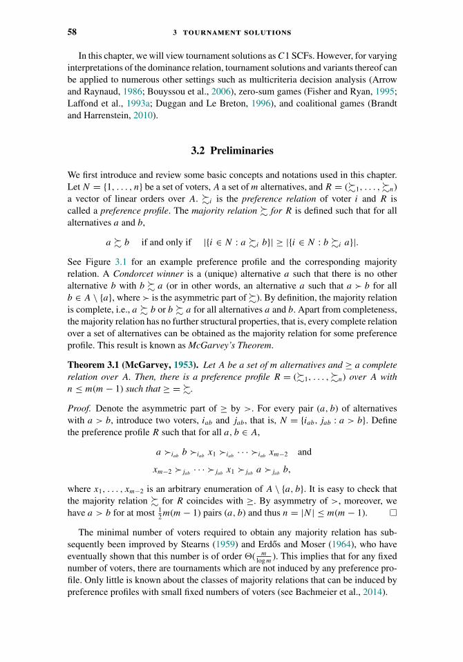
58 3 tournament solutions
In this chapter, we will view tournament solutions as C1 SCFs. However, for varyinginterpretations of the dominance relation, tournament solutions and variants thereof canbe applied to numerous other settings such as multicriteria decision analysis (Arrowand Raynaud, 1986; Bouyssou et al., 2006), zero-sum games (Fisher and Ryan, 1995;Laffond et al., 1993a; Duggan and Le Breton, 1996), and coalitional games (Brandtand Harrenstein, 2010).
3.2 Preliminaries
We first introduce and review some basic concepts and notations used in this chapter.Let N = {1, . . . , n} be a set of voters, A a set of m alternatives, and R = (�1, . . . ,�n)a vector of linear orders over A. �i is the preference relation of voter i and R iscalled a preference profile. The majority relation � for R is defined such that for allalternatives a and b,
a � b if and only if |{i ∈ N : a �i b}| ≥ |{i ∈ N : b �i a}|.See Figure 3.1 for an example preference profile and the corresponding majorityrelation. A Condorcet winner is a (unique) alternative a such that there is no otheralternative b with b � a (or in other words, an alternative a such that a � b for allb ∈ A \ {a}, where � is the asymmetric part of �). By definition, the majority relationis complete, i.e., a � b or b � a for all alternatives a and b. Apart from completeness,the majority relation has no further structural properties, that is, every complete relationover a set of alternatives can be obtained as the majority relation for some preferenceprofile. This result is known as McGarvey’s Theorem.
Theorem 3.1 (McGarvey, 1953). Let A be a set of m alternatives and ≥ a completerelation over A. Then, there is a preference profile R = (�1, . . . ,�n) over A withn ≤ m(m − 1) such that ≥ = �.
Proof. Denote the asymmetric part of ≥ by >. For every pair (a, b) of alternativeswith a > b, introduce two voters, iab and jab, that is, N = {iab, jab : a > b}. Definethe preference profile R such that for all a, b ∈ A,
a �iabb �iab
x1 �iab· · · �iab
xm−2 and
xm−2 �jab· · · �jab
x1 �jaba �jab
b,
where x1, . . . , xm−2 is an arbitrary enumeration of A \ {a, b}. It is easy to check thatthe majority relation � for R coincides with ≥. By asymmetry of >, moreover, wehave a > b for at most 1
2m(m − 1) pairs (a, b) and thus n = |N | ≤ m(m − 1).
The minimal number of voters required to obtain any majority relation has sub-sequently been improved by Stearns (1959) and Erdos and Moser (1964), who haveeventually shown that this number is of order �( m
log m). This implies that for any fixed
number of voters, there are tournaments which are not induced by any preference pro-file. Only little is known about the classes of majority relations that can be induced bypreference profiles with small fixed numbers of voters (see Bachmeier et al., 2014).
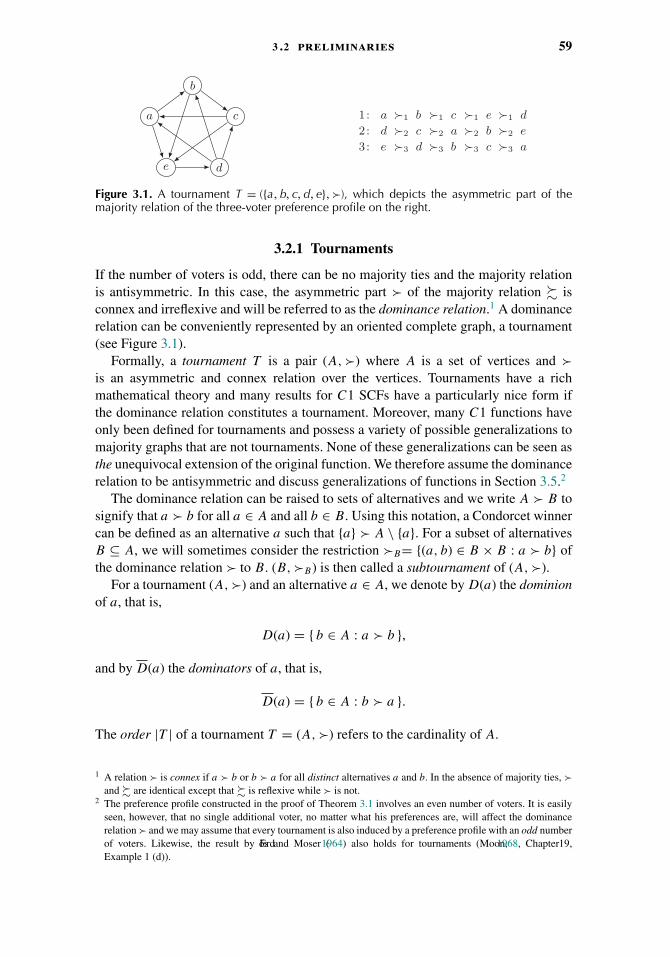
3 .2 preliminaries 59
a
b
c
de
1: a �1 b �1 c �1 e �1 d
2: d �2 c �2 a �2 b �2 e
3: e �3 d �3 b �3 c �3 a
Figure 3.1. A tournament T = ({a, b, c, d, e},�), which depicts the asymmetric part of themajority relation of the three-voter preference profile on the right.
3.2.1 Tournaments
If the number of voters is odd, there can be no majority ties and the majority relationis antisymmetric. In this case, the asymmetric part � of the majority relation � isconnex and irreflexive and will be referred to as the dominance relation.1 A dominancerelation can be conveniently represented by an oriented complete graph, a tournament(see Figure 3.1).
Formally, a tournament T is a pair (A,�) where A is a set of vertices and �is an asymmetric and connex relation over the vertices. Tournaments have a richmathematical theory and many results for C1 SCFs have a particularly nice form ifthe dominance relation constitutes a tournament. Moreover, many C1 functions haveonly been defined for tournaments and possess a variety of possible generalizations tomajority graphs that are not tournaments. None of these generalizations can be seen asthe unequivocal extension of the original function. We therefore assume the dominancerelation to be antisymmetric and discuss generalizations of functions in Section 3.5.2
The dominance relation can be raised to sets of alternatives and we write A � B tosignify that a � b for all a ∈ A and all b ∈ B. Using this notation, a Condorcet winnercan be defined as an alternative a such that {a} � A \ {a}. For a subset of alternativesB ⊆ A, we will sometimes consider the restriction �B= {(a, b) ∈ B × B : a � b} ofthe dominance relation � to B. (B,�B) is then called a subtournament of (A,�).
For a tournament (A,�) and an alternative a ∈ A, we denote by D(a) the dominionof a, that is,
D(a) = { b ∈ A : a � b },
and by D(a) the dominators of a, that is,
D(a) = { b ∈ A : b � a }.
The order |T | of a tournament T = (A,�) refers to the cardinality of A.
1 A relation � is connex if a � b or b � a for all distinct alternatives a and b. In the absence of majority ties, �and � are identical except that � is reflexive while � is not.
2 The preference profile constructed in the proof of Theorem 3.1 involves an even number of voters. It is easilyseen, however, that no single additional voter, no matter what his preferences are, will affect the dominancerelation � and we may assume that every tournament is also induced by a preference profile with an odd numberof voters. Likewise, the result by Erd os and Moser (1964) also holds for tournaments (Moon, 1968, Chapter 19,Example 1 (d)).
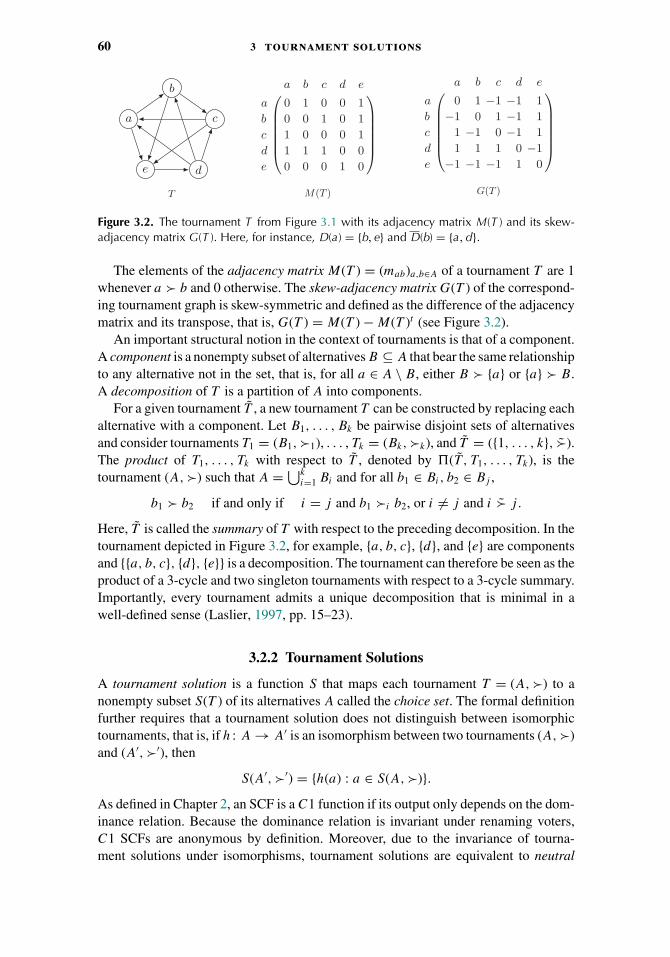
60 3 tournament solutions
T
a
b
c
de
M(T )
a b c d e
a 0 1 0 0 1
b 0 0 1 0 1
c 1 0 0 0 1
d 1 1 1 0 0
e 0 0 0 1 0
G(T )
a b c d e
a 0 1 −1 −1 1
b −1 0 1 −1 1
c 1 −1 0 −1 1
d 1 1 1 0 −1
e −1 −1 −1 1 0
Figure 3.2. The tournament T from Figure 3.1 with its adjacency matrix M(T ) and its skew-adjacency matrix G(T ). Here, for instance, D(a) = {b, e} and D(b) = {a, d}.
The elements of the adjacency matrix M(T ) = (mab)a,b∈A of a tournament T are 1whenever a � b and 0 otherwise. The skew-adjacency matrix G(T ) of the correspond-ing tournament graph is skew-symmetric and defined as the difference of the adjacencymatrix and its transpose, that is, G(T ) = M(T ) − M(T )t (see Figure 3.2).
An important structural notion in the context of tournaments is that of a component.A component is a nonempty subset of alternatives B ⊆ A that bear the same relationshipto any alternative not in the set, that is, for all a ∈ A \ B, either B � {a} or {a} � B.A decomposition of T is a partition of A into components.
For a given tournament T , a new tournament T can be constructed by replacing eachalternative with a component. Let B1, . . . , Bk be pairwise disjoint sets of alternativesand consider tournaments T1 = (B1,�1), . . . , Tk = (Bk,�k), and T = ({1, . . . , k}, �).The product of T1, . . . , Tk with respect to T , denoted by �(T , T1, . . . , Tk), is thetournament (A,�) such that A = ⋃k
i=1 Bi and for all b1 ∈ Bi, b2 ∈ Bj ,
b1 � b2 if and only if i = j and b1 �i b2, or i �= j and i � j .
Here, T is called the summary of T with respect to the preceding decomposition. In thetournament depicted in Figure 3.2, for example, {a, b, c}, {d}, and {e} are componentsand {{a, b, c}, {d}, {e}} is a decomposition. The tournament can therefore be seen as theproduct of a 3-cycle and two singleton tournaments with respect to a 3-cycle summary.Importantly, every tournament admits a unique decomposition that is minimal in awell-defined sense (Laslier, 1997, pp. 15–23).
3.2.2 Tournament Solutions
A tournament solution is a function S that maps each tournament T = (A,�) to anonempty subset S(T ) of its alternatives A called the choice set. The formal definitionfurther requires that a tournament solution does not distinguish between isomorphictournaments, that is, if h : A → A′ is an isomorphism between two tournaments (A,�)and (A′,�′), then
S(A′,�′) = {h(a) : a ∈ S(A,�)}.As defined in Chapter 2, an SCF is a C1 function if its output only depends on the dom-inance relation. Because the dominance relation is invariant under renaming voters,C1 SCFs are anonymous by definition. Moreover, due to the invariance of tourna-ment solutions under isomorphisms, tournament solutions are equivalent to neutral

3 .2 preliminaries 61
C1 functions. In contrast to Laslier (1997), we do not require tournament solutions tobe Condorcet-consistent, that is, to uniquely select a Condorcet winner whenever oneexists.
For a tournament T = (A,�) and a subset B ⊆ A, we write S(B) for the morecumbersome S(B,�B). For two tournament solutions S and S ′, we write S ′ ⊆ S, andsay that S ′ is a refinement of S and S a coarsening of S ′, if S ′(T ) ⊆ S(T ) for alltournaments T .
The literature on rational choice theory and social choice theory has identified anumber of desirable properties for (social) choice functions, also referred to as axioms,which can be readily applied to tournament solutions. In this section, we review three ofthe most important properties in this context—monotonicity, stability, and composition-consistency. As we will see in Section 3.3.2, another important property of SCFs—Pareto-optimality—is intimately connected to a particular tournament solution, theuncovered set.
A tournament solution is monotonic if a chosen alternative remains in the choice setwhen its dominion is enlarged, while leaving everything else unchanged.
Definition 3.1. A tournament solution S is monotonic if for all T = (A,�), T ′ =(A,�′), a ∈ A such that �A\{a} = �′
A\{a} and for all b ∈ A \ {a}, a �′ b whenevera � b,
a ∈ S(T ) implies a ∈ S(T ′).
Monotonicity of a tournament solution immediately implies monotonicity of thecorresponding C1 SCF. Note that this notion of monotonicity for irresolute SCFs isone of the weakest one could think of.
While monotonicity relates choices from tournaments of the same order to eachother, the next property relates choices from different subtournaments of the sametournament to each other. Informally, stability (or self-stability) requires that a set ischosen from two different sets of alternatives if and only if it is chosen from the unionof these sets.
Definition 3.2. A tournament solution S is stable if for all tournaments T = (A,�)and for all nonempty subsets B, C, X ⊆ A with X ⊆ B ∩ C,
X = S(B) = S(C) if and only if X = S(B ∪ C).
In comparison to monotonicity, stability appears to be much more demanding. It canbe factorized into two conditions, α and γ . Condition γ corresponds to the implicationfrom left to right whereas α is the implication from right to left (Brandt and Harrenstein,2011). α is also known as Chernoff’s postulate 5∗ (Chernoff, 1954), the strong supersetproperty (Bordes, 1979), outcast (Aizerman and Aleskerov, 1995), and the attentionfilter axiom (Masatlioglu et al., 2012).3 α implies idempotency,4 that is,
S(S(T )) = S(T ) for all T .
3 We refer to Monjardet (2008) for a more thorough discussion of the origins of this condition.4 Tournament solutions that fail to satisfy idempotency (such as the uncovered set) can be made idempotent by
iteratively applying the tournament solution to the resulting choice sets until no further refinement is possible.The corresponding tournament solutions, however, often violate monotonicity.
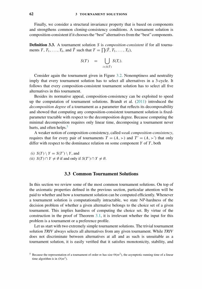
62 3 tournament solutions
Finally, we consider a structural invariance property that is based on componentsand strengthens common cloning-consistency conditions. A tournament solution iscomposition-consistent if it chooses the “best” alternatives from the “best” components.
Definition 3.3. A tournament solution S is composition-consistent if for all tourna-ments T , T1, . . . , Tk , and T such that T = ∏
(T , T1, . . . , Tk),
S(T ) =⋃
i∈S(T )
S(Ti).
Consider again the tournament given in Figure 3.2. Nonemptiness and neutralityimply that every tournament solution has to select all alternatives in a 3-cycle. Itfollows that every composition-consistent tournament solution has to select all fivealternatives in this tournament.
Besides its normative appeal, composition-consistency can be exploited to speedup the computation of tournament solutions. Brandt et al. (2011) introduced thedecomposition degree of a tournament as a parameter that reflects its decomposabilityand showed that computing any composition-consistent tournament solution is fixed-parameter tractable with respect to the decomposition degree. Because computing theminimal decomposition requires only linear time, decomposing a tournament neverhurts, and often helps.5
A weaker notion of composition-consistency, called weak composition-consistency,requires that for every pair of tournaments T = (A,�) and T ′ = (A,�′) that onlydiffer with respect to the dominance relation on some component Y of T , both
(i) S(T ) \ Y = S(T ′) \ Y , and(ii) S(T ) ∩ Y �= ∅ if and only if S(T ′) ∩ Y �= ∅.
3.3 Common Tournament Solutions
In this section we review some of the most common tournament solutions. On top ofthe axiomatic properties defined in the previous section, particular attention will bepaid to whether and how a tournament solution can be computed efficiently. Whenevera tournament solution is computationally intractable, we state NP-hardness of thedecision problem of whether a given alternative belongs to the choice set of a giventournament. This implies hardness of computing the choice set. By virtue of theconstruction in the proof of Theorem 3.1, it is irrelevant whether the input for thisproblem is a tournament or a preference profile.
Let us start with two extremely simple tournament solutions. The trivial tournamentsolution TRIV always selects all alternatives from any given tournament. While TRIVdoes not discriminate between alternatives at all and as such is unsuitable as atournament solution, it is easily verified that it satisfies monotonicity, stability, and
5 Because the representation of a tournament of order m has size �(m2), the asymptotic running time of a lineartime algorithm is in O(m2).
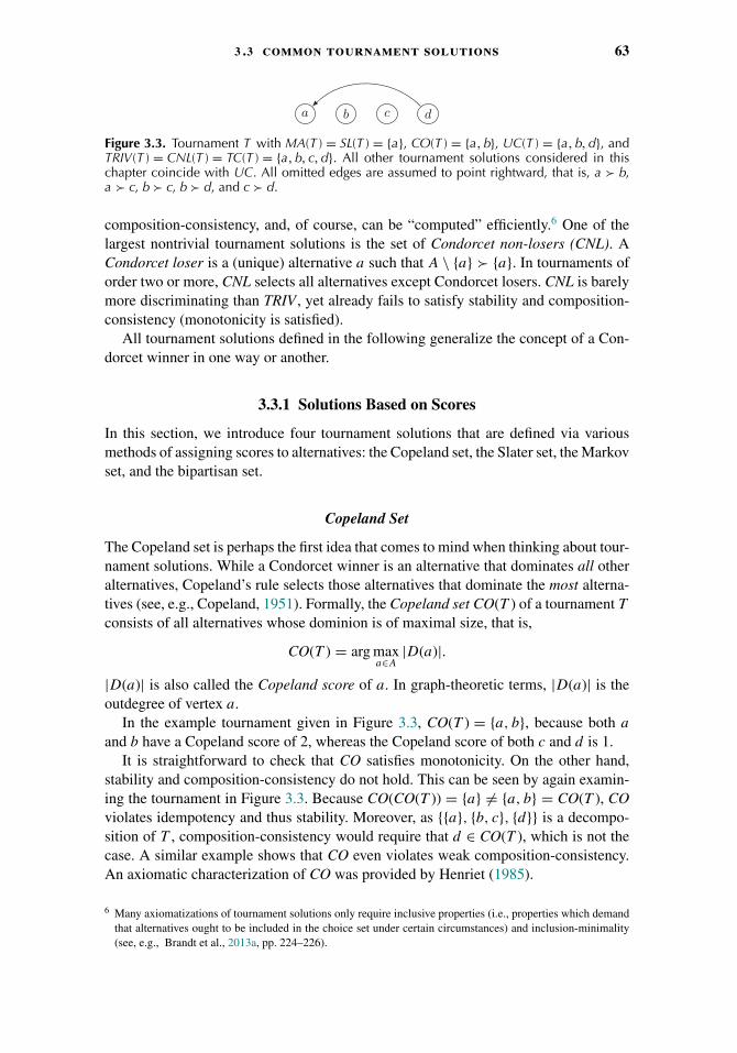
3 .3 common tournament solutions 63
a b c d
Figure 3.3. Tournament T with MA(T ) = SL(T ) = {a}, CO(T ) = {a, b}, UC(T ) = {a, b, d}, andTRIV(T ) = CNL(T ) = TC(T ) = {a, b, c, d}. All other tournament solutions considered in thischapter coincide with UC. All omitted edges are assumed to point rightward, that is, a � b,a � c, b � c, b � d, and c � d.
composition-consistency, and, of course, can be “computed” efficiently.6 One of thelargest nontrivial tournament solutions is the set of Condorcet non-losers (CNL). ACondorcet loser is a (unique) alternative a such that A \ {a} � {a}. In tournaments oforder two or more, CNL selects all alternatives except Condorcet losers. CNL is barelymore discriminating than TRIV , yet already fails to satisfy stability and composition-consistency (monotonicity is satisfied).
All tournament solutions defined in the following generalize the concept of a Con-dorcet winner in one way or another.
3.3.1 Solutions Based on Scores
In this section, we introduce four tournament solutions that are defined via variousmethods of assigning scores to alternatives: the Copeland set, the Slater set, the Markovset, and the bipartisan set.
Copeland Set
The Copeland set is perhaps the first idea that comes to mind when thinking about tour-nament solutions. While a Condorcet winner is an alternative that dominates all otheralternatives, Copeland’s rule selects those alternatives that dominate the most alterna-tives (see, e.g., Copeland, 1951). Formally, the Copeland set CO(T ) of a tournament T
consists of all alternatives whose dominion is of maximal size, that is,
CO(T ) = arg maxa∈A
|D(a)|.|D(a)| is also called the Copeland score of a. In graph-theoretic terms, |D(a)| is theoutdegree of vertex a.
In the example tournament given in Figure 3.3, CO(T ) = {a, b}, because both a
and b have a Copeland score of 2, whereas the Copeland score of both c and d is 1.It is straightforward to check that CO satisfies monotonicity. On the other hand,
stability and composition-consistency do not hold. This can be seen by again examin-ing the tournament in Figure 3.3. Because CO(CO(T )) = {a} �= {a, b} = CO(T ), COviolates idempotency and thus stability. Moreover, as {{a}, {b, c}, {d}} is a decompo-sition of T , composition-consistency would require that d ∈ CO(T ), which is not thecase. A similar example shows that CO even violates weak composition-consistency.An axiomatic characterization of CO was provided by Henriet (1985).
6 Many axiomatizations of tournament solutions only require inclusive properties (i.e., properties which demandthat alternatives ought to be included in the choice set under certain circumstances) and inclusion-minimality(see, e.g., Brandt et al., 2013a, pp. 224–226).

64 3 tournament solutions
CO can be easily computed in linear time by determining all Copeland scores andchoosing the alternatives with maximum Copeland score.7
Theorem 3.2. The Copeland set can be computed in linear time.
It is possible to define “second-order” Copeland scores by adding the Copelandscores of all alternatives within the dominion of a given alternative. The processof iteratively computing these scores is guaranteed to converge (due to the Perron-Frobenius Theorem) and leads to a tournament solution, which is sometimes referredto as the Kendall-Wei method (see, e.g., Moon, 1968, Chapter 15; Laslier, 1997, pp. 54–56). Kendall-Wei scores can be computed in polynomial time by finding the eigenvectorassociated with the largest positive eigenvalue of the adjacency matrix.
Slater Set
Although the dominance relation � of a tournament may fail to be a strict linear order,it can be linearized by inverting edges in the tournament graph. The intuition behindSlater’s rule is to select from a tournament (A,�) those alternatives that are maximalelements (i.e., Condorcet winners) in those strict linear orders that can be obtainedfrom � by inverting as few edges as possible, that is, in those strict linear orders thathave as many edges in common with � as possible (Slater, 1961).8 Thus, Slater’s rulecan be seen as the unweighted analogue of Kemeny’s social preference function (seeChapter 2 and Chapter 4).
Denote the maximal element of A according to a strict linear order > by max(>).The Slater score of a strict linear order > over the alternatives in A with respect totournament T = (A,�) is |> ∩ � |. A strict linear order is a Slater order if it hasmaximal Slater score. Then, the Slater set SL is defined as
SL(T ) = {max(>) : > is a Slater order for T }.In the example in Figure 3.3, SL(T ) = {a} because a > b > c > d is the only Slaterorder. SL satisfies monotonicity, but violates stability and composition-consistency.
Finding Slater orders is equivalent to solving an instance of the minimum feedbackarc set problem, which is known to be NP-hard, even in tournaments.9 Therefore,checking membership in SL is NP-hard as well.
Theorem 3.3 (Alon, 2006; Charbit et al., 2007; Conitzer, 2006). Deciding whetheran alternative is contained in the Slater set is NP-hard.
It is unknown whether the membership problem is contained in NP. The bestknown upper bound for this problem is the complexity class �
p2 , and Hudry (2010)
7 Brandt et al. (2009) have shown that deciding whether an alternative is contained in CO(T ) is TC0-completeand therefore not expressible in first-order logic.
8 When inverting as few edges as possible in order to obtain a Condorcet winner (rather than a strict linear order),we get the Copeland set.
9 Whether the minimum feedback arc set problem is NP-hard in tournaments was a long-standing open problemthat was solved independently by Alon (2006), Charbit et al. (2007), and Conitzer (2006). The minimumfeedback arc set problem is APX-hard (Kann, 1992) and thus does not admit a polynomial-time approximationscheme (PTAS) unless P = NP. For tournaments, however, there exists a PTAS (Kenyon-Mathieu and Schudy,2007).
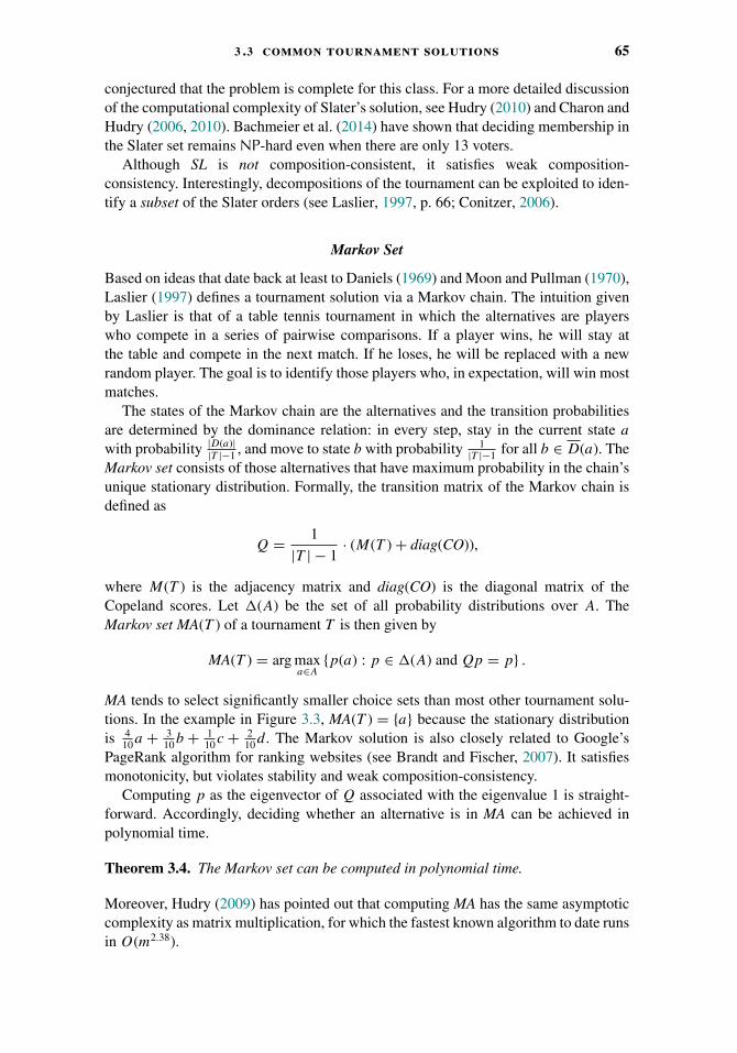
3 .3 common tournament solutions 65
conjectured that the problem is complete for this class. For a more detailed discussionof the computational complexity of Slater’s solution, see Hudry (2010) and Charon andHudry (2006, 2010). Bachmeier et al. (2014) have shown that deciding membership inthe Slater set remains NP-hard even when there are only 13 voters.
Although SL is not composition-consistent, it satisfies weak composition-consistency. Interestingly, decompositions of the tournament can be exploited to iden-tify a subset of the Slater orders (see Laslier, 1997, p. 66; Conitzer, 2006).
Markov Set
Based on ideas that date back at least to Daniels (1969) and Moon and Pullman (1970),Laslier (1997) defines a tournament solution via a Markov chain. The intuition givenby Laslier is that of a table tennis tournament in which the alternatives are playerswho compete in a series of pairwise comparisons. If a player wins, he will stay atthe table and compete in the next match. If he loses, he will be replaced with a newrandom player. The goal is to identify those players who, in expectation, will win mostmatches.
The states of the Markov chain are the alternatives and the transition probabilitiesare determined by the dominance relation: in every step, stay in the current state a
with probability |D(a)||T |−1 , and move to state b with probability 1
|T |−1 for all b ∈ D(a). TheMarkov set consists of those alternatives that have maximum probability in the chain’sunique stationary distribution. Formally, the transition matrix of the Markov chain isdefined as
Q = 1
|T | − 1· (M(T ) + diag(CO)),
where M(T ) is the adjacency matrix and diag(CO) is the diagonal matrix of theCopeland scores. Let �(A) be the set of all probability distributions over A. TheMarkov set MA(T ) of a tournament T is then given by
MA(T ) = arg maxa∈A
{p(a) : p ∈ �(A) and Qp = p} .
MA tends to select significantly smaller choice sets than most other tournament solu-tions. In the example in Figure 3.3, MA(T ) = {a} because the stationary distributionis 4
10a + 310b + 1
10c + 210d. The Markov solution is also closely related to Google’s
PageRank algorithm for ranking websites (see Brandt and Fischer, 2007). It satisfiesmonotonicity, but violates stability and weak composition-consistency.
Computing p as the eigenvector of Q associated with the eigenvalue 1 is straight-forward. Accordingly, deciding whether an alternative is in MA can be achieved inpolynomial time.
Theorem 3.4. The Markov set can be computed in polynomial time.
Moreover, Hudry (2009) has pointed out that computing MA has the same asymptoticcomplexity as matrix multiplication, for which the fastest known algorithm to date runsin O(m2.38).
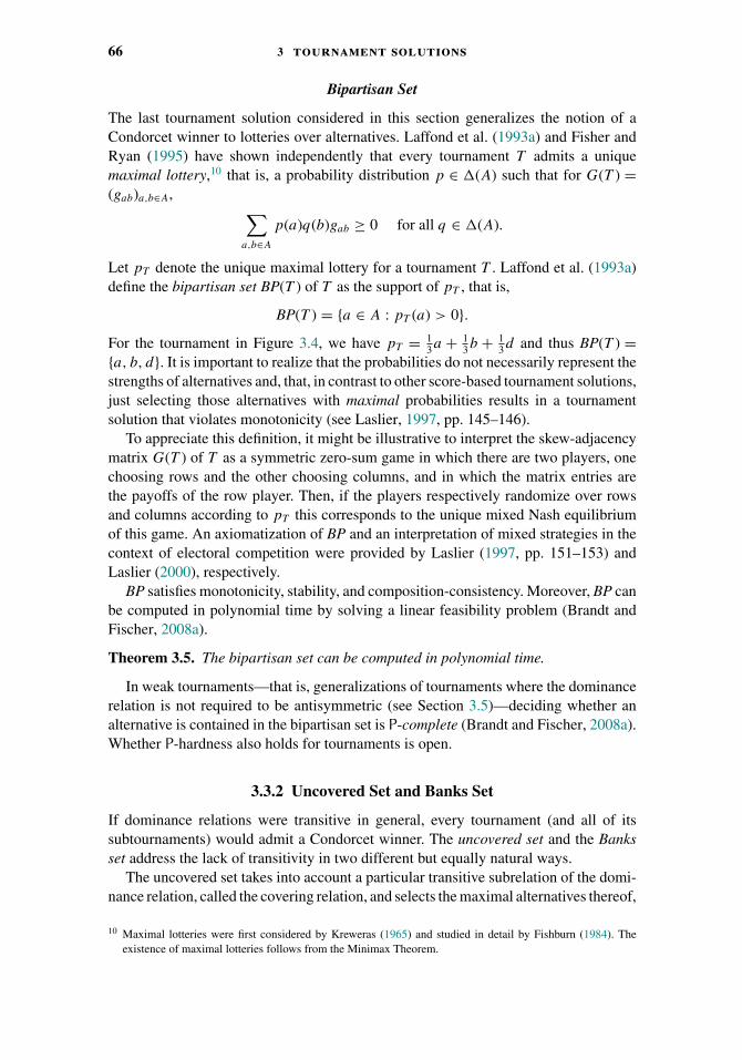
66 3 tournament solutions
Bipartisan Set
The last tournament solution considered in this section generalizes the notion of aCondorcet winner to lotteries over alternatives. Laffond et al. (1993a) and Fisher andRyan (1995) have shown independently that every tournament T admits a uniquemaximal lottery,10 that is, a probability distribution p ∈ �(A) such that for G(T ) =(gab)a,b∈A, ∑
a,b∈A
p(a)q(b)gab ≥ 0 for all q ∈ �(A).
Let pT denote the unique maximal lottery for a tournament T . Laffond et al. (1993a)define the bipartisan set BP(T ) of T as the support of pT , that is,
BP(T ) = {a ∈ A : pT (a) > 0}.For the tournament in Figure 3.4, we have pT = 1
3a + 13b + 1
3d and thus BP(T ) ={a, b, d}. It is important to realize that the probabilities do not necessarily represent thestrengths of alternatives and, that, in contrast to other score-based tournament solutions,just selecting those alternatives with maximal probabilities results in a tournamentsolution that violates monotonicity (see Laslier, 1997, pp. 145–146).
To appreciate this definition, it might be illustrative to interpret the skew-adjacencymatrix G(T ) of T as a symmetric zero-sum game in which there are two players, onechoosing rows and the other choosing columns, and in which the matrix entries arethe payoffs of the row player. Then, if the players respectively randomize over rowsand columns according to pT this corresponds to the unique mixed Nash equilibriumof this game. An axiomatization of BP and an interpretation of mixed strategies in thecontext of electoral competition were provided by Laslier (1997, pp. 151–153) andLaslier (2000), respectively.
BP satisfies monotonicity, stability, and composition-consistency. Moreover, BP canbe computed in polynomial time by solving a linear feasibility problem (Brandt andFischer, 2008a).
Theorem 3.5. The bipartisan set can be computed in polynomial time.
In weak tournaments—that is, generalizations of tournaments where the dominancerelation is not required to be antisymmetric (see Section 3.5)—deciding whether analternative is contained in the bipartisan set is P-complete (Brandt and Fischer, 2008a).Whether P-hardness also holds for tournaments is open.
3.3.2 Uncovered Set and Banks Set
If dominance relations were transitive in general, every tournament (and all of itssubtournaments) would admit a Condorcet winner. The uncovered set and the Banksset address the lack of transitivity in two different but equally natural ways.
The uncovered set takes into account a particular transitive subrelation of the domi-nance relation, called the covering relation, and selects the maximal alternatives thereof,
10 Maximal lotteries were first considered by Kreweras (1965) and studied in detail by Fishburn (1984). Theexistence of maximal lotteries follows from the Minimax Theorem.
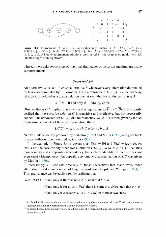
3 .3 common tournament solutions 67
a b c d e
a b c d e
a 0 1 1 −1 1
b −1 0 1 1 −1
c −1 −1 0 1 1
d 1 −1 −1 0 1
e −1 1 −1 −1 0
Figure 3.4. Tournament T and its skew-adjacency matrix G(T ). CO(T ) = SL(T ) =MA(T ) = {a}, BP = {a, b, d}, UC(T ) = BA(T ) = {a, b, c, d}, and TRIV(T ) = CNL(T ) = TC(T ) ={a, b, c, d, e}. All other tournament solutions considered in this chapter coincide with BP.Omitted edges point rightward.
whereas the Banks set consists of maximal alternatives of inclusion-maximal transitivesubtournaments.11
Uncovered Set
An alternative a is said to cover alternative b whenever every alternative dominatedby b is also dominated by a. Formally, given a tournament T = (A,�), the coveringrelation C is defined as a binary relation over A such that for all distinct a, b ∈ A,
a C b if and only if D(b) ⊆ D(a).
Observe that a C b implies that a � b and is equivalent to D(a) ⊆ D(b). It is easilyverified that the covering relation C is transitive and irreflexive, but not necessarilyconnex. The uncovered set UC(T ) of a tournament T = (A,�) is then given by the setof maximal elements of the covering relation, that is,
UC(T ) = {a ∈ A : b C a for no b ∈ A}.UC was independently proposed by Fishburn (1977) and Miller (1980) and goes backto a game-theoretic notion used by Gillies (1959).
In the example in Figure 3.4, a covers e, as D(e) = {b} and D(a) = {b, c, e}. Asthis is not the case for any other two alternatives, UC(T ) = {a, b, c, d}. UC satisfiesmonotonicity and composition-consistency, but violates stability. In fact, it does noteven satisfy idempotency. An appealing axiomatic characterization of UC was givenby Moulin (1986).
Interestingly, UC consists precisely of those alternatives that reach every otheralternative on a domination path of length at most two (Shepsle and Weingast, 1984).12
This equivalence can be easily seen by realizing that
a ∈ UC(T ) if and only if there is no b ∈ A such that b C a
if and only if for all b ∈ D(a) there is some c ∈ D(a) such that c � b
if and only if a reaches all b ∈ A \ {a} in at most two steps.
11 As Brandt (2011a) notes, the uncovered set contains exactly those alternatives that are Condorcet winners ininclusion-maximal subtournaments that admit a Condorcet winner.
12 In graph theory, these alternatives are called the kings of a tournament, and they constitute the center of thetournament graph.
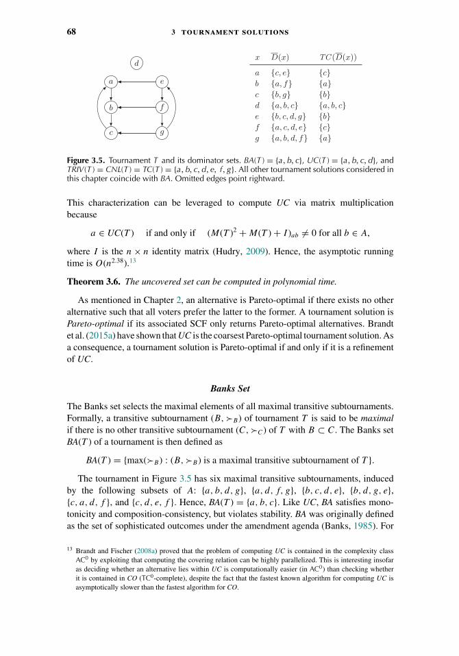
68 3 tournament solutions
a
b
c
d
e
f
g
x D(x) TC (D(x))
a {c, e} {c}b {a, f} {a}c {b, g} {b}d {a, b, c} {a, b, c}e {b, c, d, g} {b}f {a, c, d, e} {c}g {a, b, d, f} {a}
Figure 3.5. Tournament T and its dominator sets. BA(T ) = {a, b, c}, UC(T ) = {a, b, c, d}, andTRIV(T ) = CNL(T ) = TC(T ) = {a, b, c, d, e, f, g}. All other tournament solutions considered inthis chapter coincide with BA. Omitted edges point rightward.
This characterization can be leveraged to compute UC via matrix multiplicationbecause
a ∈ UC(T ) if and only if (M(T )2 + M(T ) + I )ab �= 0 for all b ∈ A,
where I is the n × n identity matrix (Hudry, 2009). Hence, the asymptotic runningtime is O(n2.38).13
Theorem 3.6. The uncovered set can be computed in polynomial time.
As mentioned in Chapter 2, an alternative is Pareto-optimal if there exists no otheralternative such that all voters prefer the latter to the former. A tournament solution isPareto-optimal if its associated SCF only returns Pareto-optimal alternatives. Brandtet al. (2015a) have shown that UC is the coarsest Pareto-optimal tournament solution. Asa consequence, a tournament solution is Pareto-optimal if and only if it is a refinementof UC.
Banks Set
The Banks set selects the maximal elements of all maximal transitive subtournaments.Formally, a transitive subtournament (B,�B) of tournament T is said to be maximalif there is no other transitive subtournament (C,�C) of T with B ⊂ C. The Banks setBA(T ) of a tournament is then defined as
BA(T ) = {max(�B) : (B,�B) is a maximal transitive subtournament of T }.The tournament in Figure 3.5 has six maximal transitive subtournaments, induced
by the following subsets of A: {a, b, d, g}, {a, d, f, g}, {b, c, d, e}, {b, d, g, e},{c, a, d, f }, and {c, d, e, f }. Hence, BA(T ) = {a, b, c}. Like UC, BA satisfies mono-tonicity and composition-consistency, but violates stability. BA was originally definedas the set of sophisticated outcomes under the amendment agenda (Banks, 1985). For
13 Brandt and Fischer (2008a) proved that the problem of computing UC is contained in the complexity classAC0 by exploiting that computing the covering relation can be highly parallelized. This is interesting insofaras deciding whether an alternative lies within UC is computationally easier (in AC0) than checking whetherit is contained in CO (TC0-complete), despite the fact that the fastest known algorithm for computing UC isasymptotically slower than the fastest algorithm for CO.
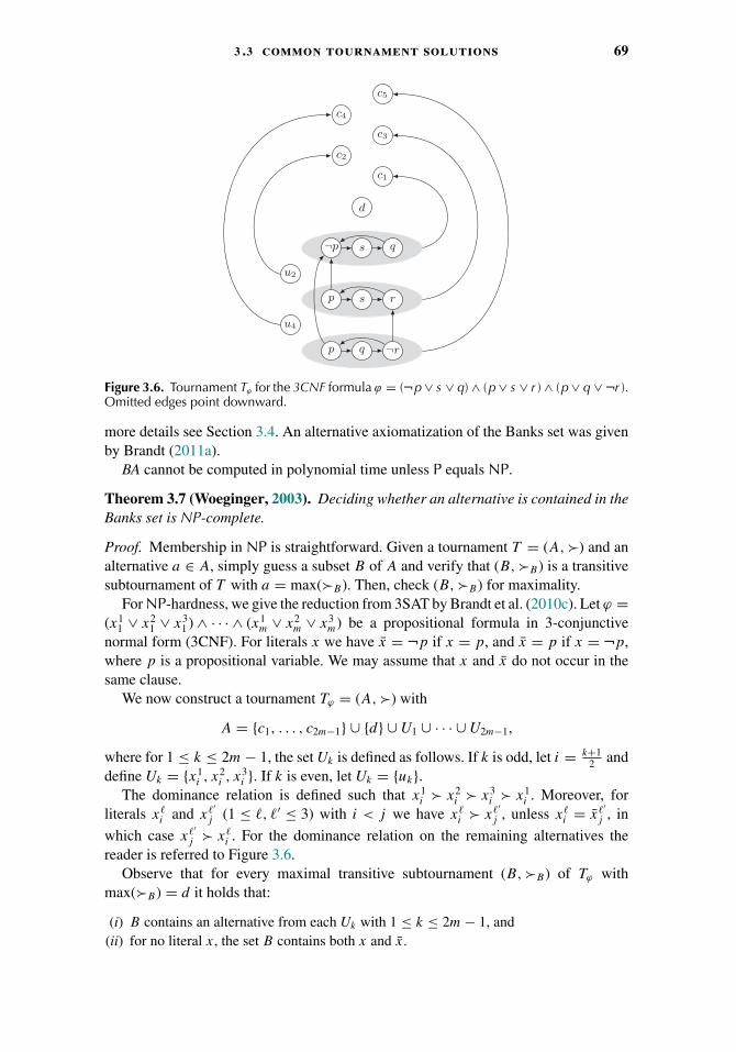
3 .3 common tournament solutions 69
p q ¬r
p s r
¬p s q
u4
u2
d
c1
c3
c5
c2
c4
Figure 3.6. Tournament Tϕ for the 3CNF formula ϕ = (¬p∨ s ∨ q) ∧ (p∨ s ∨ r ) ∧ (p∨ q ∨ ¬r ).Omitted edges point downward.
more details see Section 3.4. An alternative axiomatization of the Banks set was givenby Brandt (2011a).
BA cannot be computed in polynomial time unless P equals NP.
Theorem 3.7 (Woeginger, 2003). Deciding whether an alternative is contained in theBanks set is NP-complete.
Proof. Membership in NP is straightforward. Given a tournament T = (A,�) and analternative a ∈ A, simply guess a subset B of A and verify that (B,�B) is a transitivesubtournament of T with a = max(�B). Then, check (B,�B) for maximality.
For NP-hardness, we give the reduction from 3SAT by Brandt et al. (2010c). Let ϕ =(x1
1 ∨ x21 ∨ x3
1 ) ∧ · · · ∧ (x1m ∨ x2
m ∨ x3m) be a propositional formula in 3-conjunctive
normal form (3CNF). For literals x we have x = ¬p if x = p, and x = p if x = ¬p,where p is a propositional variable. We may assume that x and x do not occur in thesame clause.
We now construct a tournament Tϕ = (A,�) with
A = {c1, . . . , c2m−1} ∪ {d} ∪ U1 ∪ · · · ∪ U2m−1,
where for 1 ≤ k ≤ 2m − 1, the set Uk is defined as follows. If k is odd, let i = k+12 and
define Uk = {x1i , x
2i , x
3i }. If k is even, let Uk = {uk}.
The dominance relation is defined such that x1i � x2
i � x3i � x1
i . Moreover, forliterals x
i and x ′j (1 ≤ , ′ ≤ 3) with i < j we have x
i � x ′j , unless x
i = x ′j , in
which case x ′j � x
i . For the dominance relation on the remaining alternatives thereader is referred to Figure 3.6.
Observe that for every maximal transitive subtournament (B,�B) of Tϕ withmax(�B) = d it holds that:
(i) B contains an alternative from each Uk with 1 ≤ k ≤ 2m − 1, and(ii) for no literal x, the set B contains both x and x.
70 3 tournament solutions
For (i), assume that B ∩ Uk = ∅. Because max(�B) = d and cj � d for all 1 ≤ j ≤2m − 1, we have B ∩ {c1, . . . , c2m−1} = ∅. It follows that (B ∪ {ck},�B∪{ck}) is tran-sitive (ck � b for all b ∈ B), contradicting maximality of (B,�B). For (ii), assumeboth x, x ∈ B. By a previous assumption then x ∈ Uk and x ∈ Uk′ for odd k and k′
with k �= k′. Without loss of generality assume that k < k′. By (i), uk+1 ∈ B. Then,however, x � uk+1 � x � x, contradicting transitivity of (B,�B).
We now prove that
ϕ is satisfiable if and only if d ∈ BA(Tϕ).
First assume that d ∈ BA(Tϕ), that is, d = max(�B) for some maximal transitive sub-tournament (B,�B) of Tϕ . Define assignment v such that it sets propositional variable p
to true if p ∈ B and to false if ¬p ∈ B. By virtue of (ii), assignment v is well-definedand with (i) it follows that v satisfies ϕ.
For the opposite direction, assume that ϕ is satisfiable. Then, there are an assign-ment v and literals x1, . . . , xm from the clauses (x1
1 ∨ x21 ∨ x3
1 ), . . . , (x1m ∨ x2
m ∨ x3m),
respectively, such that v satisfies each of x1, . . . , xm. Define
B = {d} ∪ {x1, . . . , xm} ∪ {u2, u4, . . . , u2m−2}.It is easily seen that (B,�B) is transitive and that max(�B) = d. Observe that B
contains an alternative uk from each Uk with 1 ≤ k ≤ 2m − 1. Hence, for each ck ∈ C,we have ck � d � uk � ck and, thus, (B ∪ {ck},�B∪{ck}) is not transitive. It followsthat d = max(�B ′) for some maximal transitive subtournament (B ′,�B ′) with B ⊆ B ′,that is, d ∈ BA(Tϕ).
By modifying the construction only slightly and using a variant of 3SAT, Bach-meier et al. (2014) have shown that this problem remains NP-complete even whenthere are only 5 voters. Interestingly, finding some alternative in BA(A,�) can beachieved in linear time using the following simple procedure (Hudry, 2004). Labelthe alternatives in A as a1, . . . , am and initialize X as the empty set. Then, startingwith k = 1, successively add alternative ak to X if and only if ak dominates all alter-natives in X. After m steps, this process terminates and the last alternative added to X
can easily be seen to be a member of the Banks set. The difficulty of computing thewhole Banks set is rooted in the potentially exponential number of maximal transitivesubtournaments.
3.3.3 Solutions Based on Stability
Generalizing an idea by Dutta (1988), Brandt (2011a) proposed a method for refiningany tournament solution S by defining minimal sets that satisfy a natural stabilitycriterion with respect to S. Given a tournament solution S and a tournament T , a subsetof alternatives B ⊆ A is called S-stable in T if, for all a ∈ A \ B,
a /∈ S(B ∪ {a}).An S-stable set B is said to be minimal if there is no other S-stable set C in T suchthat C ⊂ B. Because the set of all alternatives is finite and trivially S-stable, minimalS-stable sets are guaranteed to exist. Now for each tournament solution S, there is a
3 .3 common tournament solutions 71
new tournament solution S, which returns the union of all minimal S-stable sets in atournament T = (A,�), that is,
S(T ) =⋃
{B ⊆ A : B is a minimal S-stable set in T }.A crucial issue in this context is whether S admits a unique minimal stable set in everytournament because this is necessary for S to satisfy stability (Brandt et al., 2014e).
In the following, we will define three tournament solutions using the notion of stablesets: the top cycle, the minimal covering set, and the minimal extending set.
Top Cycle
The top cycle TC can be defined as the unique minimal stable set with respect to CNL,the set of Condorcet nonlosers, that is,
TC = CNL.
Alternatively, TC can be defined via the notion of a dominant set. A nonempty subsetof alternatives B ⊆ A is called dominant in tournament T = (A,�) if B � A \ B,that is, if each alternative in B dominates all alternatives not in B. Dominant sets arelinearly ordered via set inclusion and TC returns the unique smallest dominant set. Inyet another equivalent definition, TC is defined as the set of maximal elements of thetransitive and reflexive closure of the dominance relation �. TC is a very elementarytournament solution and, in a slightly more general context (see Section 3.5), is alsoknown as weak closure maximality, GETCHA, or the Smith set (Good, 1971; Smith,1973; Schwartz, 1986). An appealing axiomatic characterization of the top cycle wasgiven by Bordes (1976).
TC tends to select rather large choice sets and may even contain Pareto-dominatedalternatives. In the example tournaments given in Figures 3.3, 3.4, and 3.5, TC selectsthe set of all alternatives because it is the only dominant set. TC satisfies monotonic-ity, stability, and weak composition-consistency, but violates the stronger notion ofcomposition-consistency (see, e.g., Figure 3.3).
Because each alternative outside TC only dominates alternatives that are also out-side TC and every alternative in TC dominates all alternatives outside TC, it can easilybe appreciated that each alternative in TC has a strictly greater Copeland score thaneach alternative outside TC. Hence, CO ⊆ TC.
Exploiting this insight, TC(T ) can be computed in linear time by starting with CO(T )and then iteratively adding alternatives that are not dominated by the current set.Alternatively, one can employ an algorithm, for example, the Kosaraju-Sharir algorithmor Tarjan’s algorithm, for finding the strongly connected components of T and thenoutput the unique strongly connected component that dominates all other stronglyconnected components.14
Theorem 3.8. The top cycle can be computed in linear time.
14 Brandt et al. (2009) have shown that the problem of deciding whether an alternative is contained in the topcycle of a tournament is in the complexity class AC0.
72 3 tournament solutions
Minimal Covering Set
A subset B of alternatives is called a covering set if it is UC-stable, that is, if everya ∈ A \ B is covered in the subtournament (B ∪ {a},�B∪{a}). The minimal coveringset MC is defined as
MC = UC.
Dutta (1988) has shown that every tournament admits a unique minimal UC-stableset and that MC ⊆ UC. In the example in Figure 3.4, MC(T ) = {a, b, d}, and henceMC is a strict refinement of UC. Observe that, for instance, {a, b, c} is not UC-stable, as d ∈ UC({a, b, c, d}). MC satisfies monotonicity, stability, and composition-consistency. Dutta also provided an axiomatic characterization of MC, which was laterimproved by Laslier (1997, pp. 117–120).
Laffond et al. (1993a) have shown that BP ⊆ MC. By virtue of Theorem 3.5, wecan therefore efficiently compute a nonempty subset of MC. This fact can be used tocompute MC by leveraging the following lemma.
Lemma 3.9. Let T = (A,�) be a tournament and B ⊆ MC(A). Define C = {a ∈A \ B : a ∈ UC(B ∪ {a})}. Then, MC(C) ⊆ MC(A).
MC(T ) can then be computed by first computing the bipartisan set BP(T ) and theniteratively adding a specific subset of alternatives that lie outside the current set but dobelong to MC(T ). Lemma 3.9 tells us how this subset can be found at each stage (seeAlgorithm 1).15
Algorithm 1 Minimal covering setprocedure MC(A,�)
B ← BP(A)loop
C ← {a ∈ A \ B : a ∈ UC(B ∪ {a}}if C = ∅ then return B end ifB ← B ∪ BP(C)
end loop
Theorem 3.10 (Brandt and Fischer, 2008a). The minimal covering set can be com-puted in polynomial time.
Minimal Extending Set
A subset of alternatives is called an extending set if it is BA-stable. Brandt (2011a)defined the minimal extending set ME(T ) as the union of all minimal extending sets ofa tournament T , that is,
ME = BA.
15 Lemma 3.9 can also be used to construct a recursive algorithm for computing MC without making referenceto BP. However, such an algorithm has exponential worst-case running time.
3 .3 common tournament solutions 73
In the tournament in Figure 3.4, we find that ME(T ) = {a, b, d}. Brandt et al. (2014c)showed that ME ⊆ BA and that computing ME is computationally intractable by usinga construction similar to that of the proof of Theorem 3.7.
Theorem 3.11 (Brandt et al., 2014c). Deciding whether an alternative is containedin a minimal extending set is NP-hard.
The best known upper bound for this decision problem is the complexity class �p3 .
Bachmeier et al. (2014) have shown that the problem remains NP-hard even whenthere are only 7 voters. A relation-algebraic specification of minimal extendingsets, which can be used to compute ME on small instances, was proposed byBerghammer (2014).
Brandt (2011a) proved that ME satisfies composition-consistency, and conjecturedthat every tournament contains a unique minimal extending set. Even though thisconjecture was later disproved, which implies that ME violates monotonicity andstability, it is unclear whether this seriously impairs the usefulness of ME (Brandtet al., 2013b, 2014c). The counterexample found by Brandt et al. consists of about10136 alternatives and concrete tournaments for which ME violates any of theseproperties have never been encountered (even when resorting to extensive computerexperiments).
3.3.4 Solutions Based on Retentiveness
Finally, we consider an operator on tournament solutions which bears some resem-blance to the notion of minimal stable sets as introduced in the previous section. Theunderlying idea of retentiveness was first proposed by Schwartz (1990) and studiedmore generally by Brandt et al. (2014d).
For a given tournament solution S, we say that an alternative a is S-dominated byalternative b if b is chosen among a’s dominators by S. Similarly, a nonempty setof alternatives is called S-retentive if none of its elements is S-dominated by somealternative outside the set. Formally, for a tournament solution S and a tournamentT = (A,�), a nonempty subset B ⊆ A is S-retentive in T if for all b ∈ B such thatD(b) �= ∅,
S(D(b)) ⊆ B.
An S-retentive set B in T is said to be minimal if there is no other S-retentiveset C in T with C ⊂ B. As in the case of S-stable sets, minimal S-retentive sets areguaranteed to exist because the set of all alternatives is trivially S-retentive. Thus wecan define S as the tournament solution yielding the union of minimal S-retentive sets,that is, for all tournaments T = (A,�),
S(T ) =⋃
{B ⊆ A : B is a minimal S-retentive set in T }.
As with minimal stable sets, it is important for the axiomatic properties of S whetherS admits a unique minimal retentive set in every tournament. It is easily veri-fied that there always exists a unique minimal TRIV-retentive set, and that in fact
˚TRIV = TC.
74 3 tournament solutions
The Minimal TC-Retentive Set
Brandt et al. (2014d) have shown that S inherits several desirable properties from S—including monotonicity and stability—whenever a unique minimal S-retentive set isguaranteed to exist. They went on to show that every tournament admits a uniqueTC-retentive set. As a consequence, the tournament solution TC—which can also be
written as ˚TRIV—is monotonic and stable. Also, TC inherits efficient computabilityfrom TC and satisfies weak composition-consistency.
Theorem 3.12 (Brandt et al., 2014d). The minimal TC-retentive set can be computedin polynomial time.
In the tournament in Figure 3.5, the set {a, b, c} and each of its supersets is TC-retentive. Therefore, TC(T ) = {a, b, c}.
Tournament Equilibrium Set
Schwartz (1990) defined the tournament equilibrium set (TEQ) recursively as the unionof all minimal TEQ-retentive sets,
TEQ = ˚TEQ.
This recursion is well-defined because the order of the dominator set of any alternativeis strictly smaller than the order of the original tournament. In the example in Figure 3.5,TEQ(T ) = TC(T ) = {a, b, c}, because TEQ and TC coincide on all dominator sets.
TEQ is the only tournament solution defined via retentiveness that satisfiescomposition-consistency. Schwartz conjectured that every tournament contains aunique minimal TEQ-retentive set. As was shown by Laffond et al. (1993b) and Houy(2009b,a), TEQ satisfies any one of a number of important properties including mono-tonicity and stability if and only if Schwartz’s conjecture holds. Brandt et al. (2013b)showed that Schwartz’s conjecture does not hold by nonconstructively disproving arelated weaker conjecture surrounding ME.16 As a consequence, TEQ violates mono-tonicity and stability. However, counterexamples to Schwartz’s conjecture appear to beextremely rare and it may be argued that TEQ satisfies the properties for all practicalpurposes.
Using a construction similar to that of the proof of Theorem 3.7, it can be shownthat computing TEQ is intractable.17
Theorem 3.13 (Brandt et al., 2010c). Deciding whether an alternative is containedin the tournament equilibrium set is NP-hard.
There is no obvious reason why checking membership in TEQ should be in NP. Thebest known upper bound for this problem is the complexity class PSPACE. Bachmeier
16 A significantly smaller counterexample for Schwartz’s conjecture, consisting of only 24 alternatives, was foundby Brandt and Seedig (2013). However, this smaller counterexample does not disprove the correspondingconjecture for ME.
17 The proof of Theorem 3.13 actually shows that the membership decision problem for any tournament solutionthat is sandwiched between BA and TEQ, that is, computing any tournament solution S with TEQ ⊆ S ⊆ BA,is NP-hard.
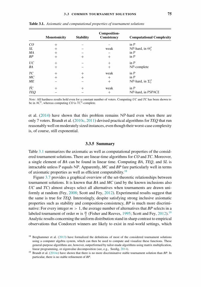
3 .3 common tournament solutions 75
Table 3.1. Axiomatic and computational properties of tournament solutions
Composition-Monotonicity Stability Consistency Computational Complexity
CO + – – in PSL + – weak NP-hard, in �
p2
MA + – – in PBP + + + in P
UC + – + in PBA + – + NP-complete
TC + + weak in PMC + + + in PME – – + NP-hard, in �
p3
TC + + weak in PTEQ – – + NP-hard, in PSPACE
Note: All hardness results hold even for a constant number of voters. Computing UC and TC has been shown tobe in AC0, whereas computing CO is TC0-complete.
et al. (2014) have shown that this problem remains NP-hard even when there areonly 7 voters. Brandt et al. (2010c, 2011) devised practical algorithms for TEQ that runreasonably well on moderately sized instances, even though their worst-case complexityis, of course, still exponential.
3.3.5 Summary
Table 3.1 summarizes the axiomatic as well as computational properties of the consid-ered tournament solutions. There are linear-time algorithms for CO and TC. Moreover,a single element of BA can be found in linear time. Computing BA, TEQ, and SL isintractable unless P equals NP. Apparently, MC and BP fare particularly well in termsof axiomatic properties as well as efficient computability.18
Figure 3.7 provides a graphical overview of the set-theoretic relationships betweentournament solutions. It is known that BA and MC (and by the known inclusions alsoUC and TC) almost always select all alternatives when tournaments are drawn uni-formly at random (Fey, 2008; Scott and Fey, 2012). Experimental results suggest thatthe same is true for TEQ. Interestingly, despite satisfying strong inclusive axiomaticproperties such as stability and composition-consistency, BP is much more discrimi-native: For every integer m > 1, the average number of alternatives that BP selects in alabeled tournament of order m is m
2 (Fisher and Reeves, 1995; Scott and Fey, 2012).19
Analytic results concerning the uniform distribution stand in sharp contrast to empiricalobservations that Condorcet winners are likely to exist in real-world settings, which
18 Berghammer et al. (2013) have formalized the definitions of most of the considered tournament solutionsusing a computer algebra system, which can then be used to compute and visualize these functions. Thesegeneral-purpose algorithms are, however, outperformed by tailor-made algorithms using matrix multiplication,linear programming, or eigenvalue decomposition (see, e.g., Seedig, 2014).
19 Brandt et al. (2014e) have shown that there is no more discriminative stable tournament solution than BP. Inparticular, there is no stable refinement of BP.

76 3 tournament solutions
TC
UC
BA
MC
ME
TEQ
BPSL MA
CO
Figure 3.7. The set-theoretic relationships between tournament solutions are depicted in thisVenn-like diagram. If the ellipses of two tournament solutions S and S′ intersect, then S(T ) ∩S′(T ) �= ∅ for all tournaments T . If the ellipses for S an S′ are disjoint, however, this signifiesthat S(T ) ∩ S′(T ) = ∅ for some tournament T . Thus, BA and MC are not included in each other,but they always have a nonempty intersection (see, e.g., Laslier, 1997). CO, MA, and SL arecontained in UC but may be disjoint from MC and BA. The exact location of BP in this diagramis unknown, but it intersects with TEQ in all known instances and is contained in MC. TEQ andME are contained in BA, but their inclusion in MC is uncertain. Hence, the ellipses for TEQ,ME, and BP are dashed. TC is omitted in this figure because very little is known apart from theinclusion in TC (see Brandt et al., 2015b, for more details).
implies that tournament solutions are much more discriminative than these analyticalresults suggest (Brandt and Seedig, 2015).
3.4 Strategyproofness and Agenda Implementation
It is well-known from the Gibbard-Satterthwaite Theorem (see Chapter 2) that onlytrivial resolute SCFs are strategyproof, that is, immune against the strategic misrepre-sentation of preferences. Tournament solutions are irresolute by definition (think of a3-cycle) and therefore the Gibbard-Satterthwaite Theorem does not apply directly.20
There are two ways to obtain weak forms of strategyproofness that are partic-ularly well-suited for tournament solutions. The first one concerns the traditionalnotion of strategyproofness with respect to weakly dominant strategies, but incom-plete preference relations over sets of alternatives, and the second one deals with theimplementation of tournament solutions by means of sequential binary agendas andsubgame-perfect Nash equilibrium. Each of these methods allows for rather positiveresults, but also comes at a cost: the first one requires a high degree of uncertainty
20 However, the Gibbard-Satterthwaite Theorem does imply that no resolute refinement of any of the tournamentsolutions discussed in this chapter—except TRIV—is strategyproof. There are important extensions of theGibbard-Satterthwaite Theorem to irresolute SCFs such as the Duggan-Schwartz Theorem (see Chapter 2).We will focus on more positive results for tournament solutions in this chapter.

3 .4 strategyproofness and agenda implementation 77
among the voters as to how ties are broken, whereas the second one requires commonknowledge of all preferences and may result in impractical voting procedures.
3.4.1 Strategyproofness
A proper definition of strategyproofness for irresolute SCFs requires the specificationof preferences over sets of alternatives. One way to obtain such preferences is toextend the preferences that voters have over individual alternatives to (not necessarilycomplete) preference relations over sets. A function that yields a preference relationover subsets of alternatives when given a preference relation over single alternatives iscalled a set extension. Of course, there are various set extensions, each of which leadsto a different class of strategyproof SCFs (see, e.g., Gardenfors, 1979; Barbera et al.,2004; Taylor, 2005, Brandt, 2015; Brandt and Brill, 2011).
Here, we will concentrate on two natural and well-studied set extensions due toKelly (1977) and Fishburn (1972), respectively.21 Let �i be the preference relation ofvoter i and let B and C be two nonempty sets of alternatives. Then, Kelly’s extensionis defined by letting
B �Ki C if and only if b �i c for all b ∈ B and c ∈ C.
One interpretation of this extension is that voters are completely unaware of thetiebreaking mechanism (e.g., a lottery) that will be used to pick the winning alter-native.
Fishburn’s extension is defined by letting
B �Fi C if and only if b �i c for all b ∈ B and c ∈ C \ B and
b �i c for all b ∈ B \ C and c ∈ C.
One interpretation of this extension is that ties are broken according to some unknownlinear order (e.g., the preferences of a chairman). It is easily seen that B �K
i C impliesB �F
i C.Each set extension induces a corresponding notion of strategyproofness. An SCF f
is Kelly-strategyproof if there is no voter i and no pair of preference profiles R and R′
with �j=�′j for all j �= i such that f (R′) �K
i f (R). If such profiles exist, we say thatvoter i can manipulate f . Fishburn-strategyproofness is defined analogously. Note thatin this definition of strategyproofness, set extensions are interpreted as fully specifiedpreference relations according to which many choice sets are incomparable (and chang-ing the outcome to an incomparable choice set does not constitute a manipulation).Clearly, because B �K
i C implies B �Fi C, Fishburn-strategyproofness is stronger
than Kelly-strategyproofness.Kelly-strategyproofness may seem like an extremely weak notion of strategyproof-
ness as only few pairs of sets can actually be compared. Nevertheless, almost allcommon SCFs fail to satisfy Kelly-strategyproofness because they can already bemanipulated on profiles where these functions are resolute (Taylor, 2005, pp. 44–51).
21 Gardenfors (1979) attributed the second extension to Fishburn because it is the coarsest extension that satisfiesa certain set of axioms proposed by Fishburn (1972).

78 3 tournament solutions
Brandt (2015) has shown that stability and monotonicity are sufficient for Kelly-strategyproofness. Virtually all SCFs of interest that satisfy these conditions are tour-nament solutions (or weighted tournament solutions). We therefore only state the resultfor tournament solutions rather than for SCFs.
Theorem 3.14 (Brandt, 2015). Every monotonic and stable tournament solutionis Kelly-strategyproof. Moreover, every Condorcet-consistent coarsening of a Kelly-strategyproof tournament solution is Kelly-strategyproof.
As a consequence, BP, each of its Condorcet-consistent coarsenings (such as MC,UC, and TC), and TC are Kelly-strategyproof.22 On the other hand, it can be shown thatevery Condorcet-consistent tournament solution that may return a single alternative inthe absence of a Condorcet winner is Kelly-manipulable. It follows that CO, SL, andMA fail to be Kelly-strategyproof. More involved arguments can be used to show thatME and TEQ are not Kelly-strategyproof.
The results for Fishburn-strategyproofness are less encouraging. While it is knownthat TC is Fishburn-strategyproof (Brandt and Brill, 2011; Sanver and Zwicker, 2012),a computer-aided proof has shown that no refinement of UC is Fishburn-strategyproof.Because UC is the coarsest Pareto-optimal tournament solution, we have the followingtheorem.
Theorem 3.15 (Brandt and Geist, 2014). There is no Pareto-optimal Fishburn-strategyproof tournament solution.
As a consequence of this theorem, the set-theoretic relationships depicted inFigure 3.7, and other observations (Brandt and Brill, 2011), TC is the finest Fishburn-strategyproof tournament solution considered in this chapter.
3.4.2 Agenda Implementation
An important question—which has enjoyed considerable attention from social choicetheorists and political scientists since the work of Black (1958) and Farquharson(1969)—is whether simple procedures exists that implement a particular tournamentsolution. This in particular concerns procedures that are based on a series of binarychoices and eventually lead to the election of a single alternative. The binary choicesmay depend on one another and need not exclusively be between two alternatives. Suchprocedures are in wide use by actual committees and institutions at various levels ofdemocratic decision making. The most prominent among these are the simple agenda(or successive procedure) and the amendment procedure, both of which were initiallystudied in their own right by political scientists. The former is prevalent in civil law orEuro-Latin legal systems, whereas the latter is more firmly entrenched in the commonlaw or Anglo-American legal tradition (see, e.g., Apesteguia et al., 2014).
With the simple agenda, the alternatives are ordered in a sequence a1, . . . , am andsubsequently successively being voted up or down by majority voting: First alterna-tive a1 is brought up for consideration; if a1 is carried by a majority, it is accepted as
22 In fact, the proof even shows that these functions are group-strategyproof with respect to Kelly’s extension.
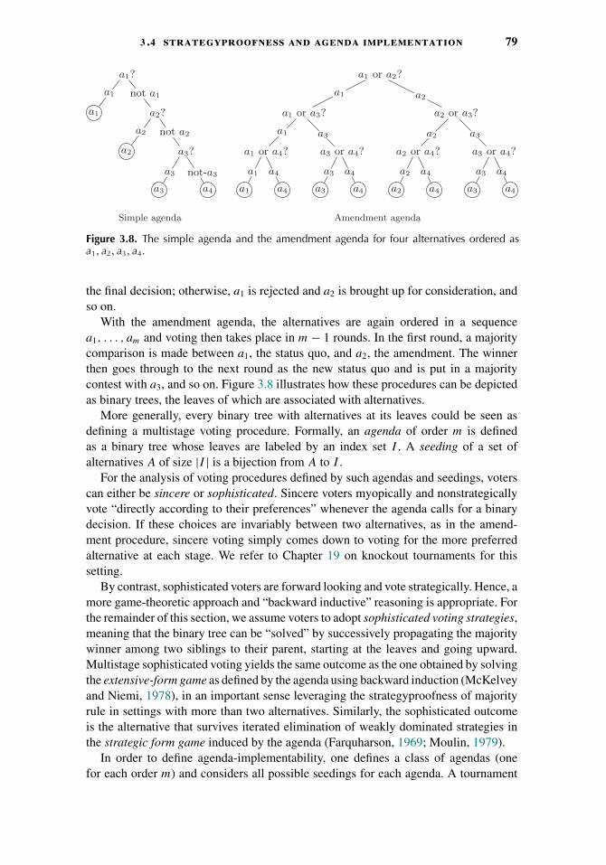
3 .4 strategyproofness and agenda implementation 79
Simple agenda
a1?
a2?
a3?
a4a3
a3 not-a3
a2
a2 not a2
a1
a1 not a1
Amendment agenda
a1 or a2?
a2 or a3?
a3 or a4?
a4a3
a3 a4
a2 or a4?
a4a2
a2 a4
a2 a3
a1 or a3?
a3 or a4?
a4a3
a3 a4
a1 or a4?
a4a1
a1 a4
a1 a3
a1 a2
Figure 3.8. The simple agenda and the amendment agenda for four alternatives ordered asa1, a2, a3, a4.
the final decision; otherwise, a1 is rejected and a2 is brought up for consideration, andso on.
With the amendment agenda, the alternatives are again ordered in a sequencea1, . . . , am and voting then takes place in m − 1 rounds. In the first round, a majoritycomparison is made between a1, the status quo, and a2, the amendment. The winnerthen goes through to the next round as the new status quo and is put in a majoritycontest with a3, and so on. Figure 3.8 illustrates how these procedures can be depictedas binary trees, the leaves of which are associated with alternatives.
More generally, every binary tree with alternatives at its leaves could be seen asdefining a multistage voting procedure. Formally, an agenda of order m is definedas a binary tree whose leaves are labeled by an index set I . A seeding of a set ofalternatives A of size |I | is a bijection from A to I .
For the analysis of voting procedures defined by such agendas and seedings, voterscan either be sincere or sophisticated. Sincere voters myopically and nonstrategicallyvote “directly according to their preferences” whenever the agenda calls for a binarydecision. If these choices are invariably between two alternatives, as in the amend-ment procedure, sincere voting simply comes down to voting for the more preferredalternative at each stage. We refer to Chapter 19 on knockout tournaments for thissetting.
By contrast, sophisticated voters are forward looking and vote strategically. Hence, amore game-theoretic approach and “backward inductive” reasoning is appropriate. Forthe remainder of this section, we assume voters to adopt sophisticated voting strategies,meaning that the binary tree can be “solved” by successively propagating the majoritywinner among two siblings to their parent, starting at the leaves and going upward.Multistage sophisticated voting yields the same outcome as the one obtained by solvingthe extensive-form game as defined by the agenda using backward induction (McKelveyand Niemi, 1978), in an important sense leveraging the strategyproofness of majorityrule in settings with more than two alternatives. Similarly, the sophisticated outcomeis the alternative that survives iterated elimination of weakly dominated strategies inthe strategic form game induced by the agenda (Farquharson, 1969; Moulin, 1979).
In order to define agenda-implementability, one defines a class of agendas (onefor each order m) and considers all possible seedings for each agenda. A tournament

80 3 tournament solutions
solution S is then said to be agenda-implementable if there exists a class of agendassuch that for every tournament T , a ∈ S(T ) if and only if there is a seeding for theagenda of size |T | such that its sophisticated outcome is a.
Early results on agenda implementation demonstrated that the class of simple agen-das implements TC and the class of amendment agendas implements BA (Miller, 1977,1980; Banks, 1985; Moulin, 1986). Moulin (1986), moreover, showed that agenda-implementable tournament solutions have to be weakly composition-consistent refine-ments of TC. As a consequence, CO and MA are not agenda-implementable. A com-plete characterization of agenda-implementable tournament solutions, however, hadlong remained elusive before Horan (2013) obtained sufficient conditions for agenda-implementability that cover a wide range of tournament solutions and almost matchMoulin’s necessary conditions.23
Theorem 3.16 (Horan, 2013). Every weakly composition-consistent tournamentsolutions that chooses from among the top cycle of every component is agenda-implementable.
As a corollary to this result it follows that—besides TC and BA—also SL, UC,MC, ME, BP, and TEQ are agenda-implementable. It should be observed, however,that the agendas actually implementing these tournament solutions may be extremelylarge. The size of the amendment agenda, for instance, is already exponential inthe number of alternatives.24 Moreover, Horan’s proof is nonconstructive and noconcrete classes of agendas that implement any of the tournament solutions con-sidered in this chapter—except the simple agenda and the amendment agenda—areknown.
The fact that CO fails to be agenda-implementable has sparked some research onapproximating Copeland winners via binary agendas. Fischer et al. (2011) showedthat agenda-implementability is unachievable for any tournament solution that, fromtournaments of order m, only chooses alternatives with a Copeland score at least ashigh as 3
4 + O( 1m
) of the maximum Copeland score. Horan (2013) demonstrated theexistence of agenda-implementable tournament solutions that only select alternativeswhose Copeland score is at least 2
3 of the maximum Copeland score, improving previousresults by Fischer et al. (2011).
3.4.3 Summary
Table 3.2 summarizes which of the considered tournament solutions are Kelly-strategyproof, Fishburn-strategyproof, and agenda-implementable, respectively. Again,it turns out that BP represents a decent compromise between discriminative power andattractive axiomatic properties.
23 A weaker version of Theorem 3.16 simply states that every composition-consistent refinement of TC is agenda-implementable.
24 As an extreme case consider the agendas that Coughlan and Le Breton (1999) introduced to implement arefinement of the iterated Banks set (see also Laslier, 1997). The corresponding agenda of order 6 has already2720! − 1 nodes!

3 .5 generalizations to weak tournaments 81
Table 3.2. Strategic properties of tournament solutions
Kelly- Fishburn- Agenda-Strategyproofness Strategyproofness Implementability
CO – – –SL – – +MA – – –BP + – +UC + – +BA ? – + (amendment)
TC + + + (simple)MC + – +ME – – +TC + – ?TEQ – – +
Note: It is unknown whether BA is Kelly-strategyproof and whether TC is agenda-implementable.Interestingly, TC falls exactly between the necessary and sufficient conditions given by Moulin(1986) and Horan (2013).
3.5 Generalizations to Weak Tournaments
So far, we assumed the majority relation to be antisymmetric, which can be justified,for instance, by assuming that there is an odd number of voters. In general, however,there may be majority ties. These can be accounted for by considering weak tourna-ments (A,�), that is, directed graphs that represent the complete, but not necessarilyantisymmetric, majority relation.25
For most of the tournament solutions defined in Section 3.3, generalizations orextensions to weak tournaments have been proposed. Often, it turns out that there areseveral sensible ways to generalize a tournament solution and it is unclear whetherthere exists a unique “correct” generalization. A natural criterion for evaluating thedifferent proposals is whether the extension satisfies (appropriate generalizations of)the axiomatic properties that the original tournament solution satisfies.
3.5.1 The Conservative Extension
A generic way to generalize any given tournament solution S to weak tournamentsis by selecting all alternatives that are chosen by S in some orientation of the weaktournament. Formally, a tournament T = (A,�) is an orientation of a weak tournamentW = (A,�′) if a � b implies a �′ b for all a, b ∈ A. The conservative extension ofS, denoted [S], is defined such that, for every weak tournament W ,
[S](W ) =⋃
T ∈[W ]
S(T ),
25 Alternatively, one can consider the strict part of the majority relation�, which is asymmetric, but not necessarilyconnex.

82 3 tournament solutions
where [W ] denotes the set of all orientations of W . Brandt et al. (2014a) have shownthat [S] inherits several natural properties from S, including monotonicity, stability,and composition-consistency.
An alternative interpretation of weak tournaments is in terms of a partial informationsetting, where the symmetric and irreflexive part of the dominance relation representsunknown comparisons rather than actual ties (see Chapter 10). In this setting, the setof winners according to the conservative extension exactly corresponds to the set ofpossible winners of the partially specified tournament. The computational complexityof possible and necessary winners of partially specified tournaments has been studiedby Aziz et al. (2012b), who showed that for a number of tractable tournament solutions(such as CO, UC, and TC), possible winners—and thus the conservative extension—canbe computed efficiently.
3.5.2 Extensions of Common Tournament Solutions
For many tournament solutions, ad hoc extensions have been proposed in the literature.In this section, we give an overview of these extensions and compare them to theconservative extension.
The Copeland set CO gives rise to a whole class of extensions that is parameterizedby a number α between 0 and 1. The solution COα selects all alternatives that maximizethe variant of the Copeland score in which each tie contributes α points to an alterna-tive’s score (see, e.g., Faliszewski et al. (2009c)). Henriet (1985) axiomatically charac-terized CO
12 , arguably the most natural variant in this class. The conservative extension
[CO] does not coincide with any of these solutions. Furthermore, [CO] �⊆ COα for allα ∈ [0, 1] and COα ⊆ [CO] if and only if 1
2 ≤ α ≤ 1.When moving from tournaments to weak tournaments, maximal lotteries are no
longer unique. Dutta and Laslier (1999) have shown that the appropriate generalizationof the bipartisan set BP is the essential set ES, which is given by the set of all alternativesthat are contained in the support of some maximal lottery. The essential set coincideswith the support of any quasi-strict Nash equilibrium of the game defined by theskew-adjacency matrix. It is easy to construct tournaments where ES is strictly smallerthan [BP], and there are also weak tournaments in which [BP] is strictly containedin ES.
Duggan (2013) surveyed several extensions of the covering relation to weak tour-naments. Any such relation induces a generalization of the uncovered set UC. Theso-called deep covering and McKelvey covering relations are particularly interestingextensions. Duggan showed that for all other generalizations of the covering relationhe considered, the corresponding uncovered set is a refinement of the deep uncoveredset UCD. Another interesting property of UCD is that it coincides with the conservativeextension of UC. It follows that all other UC generalizations considered by Dugganare refinements of [UC].
Banks and Bordes (1988) discussed four different generalizations of the Banks set BAto weak tournaments. Each of these generalizations is a refinement of the conservativeextension [BA].
For the top cycle TC, Schwartz (1972; 1986) defined two different generalizations(see also Sen, 1986). GETCHA (or the Smith set) contains the maximal elements of the
3 .6 further reading 83
transitive closure of �, whereas GOCHA (or the Schwartz set) contains the maximalelements of the transitive closure of �. GOCHA is always contained in GETCHA,and the latter coincides with [TC]. A game-theoretical interpretation of TC givesrise to a further generalization. Duggan and Le Breton (2001) observed that the topcycle of a tournament T coincides with the unique mixed saddle MS(T ) of the gameG(T ), and showed that the mixed saddle is still unique for games corresponding toweak tournaments. The solution MS is nested between GOCHA and GETCHA. Thecomputational complexity of GETCHA and GOCHA was analyzed by Brandt et al.(2009), and the complexity of mixed saddles was studied by Brandt and Brill (2012).
Generalizations of the minimal covering set MC using the McKelvey coveringrelation and the deep covering relation are known to satisfy stability. There existweak tournaments in which [MC] is strictly contained in both the McKelvey minimalcovering set MCM and the deep minimal covering set MCD. There are also weaktournaments in which MCM is strictly contained in [MC]. Computational aspects ofgeneralized minimal covering sets have been analyzed by Brandt and Fischer (2008a)and Baumeister et al. (2013a).
Schwartz (1990) suggested six ways to extend the tournament equilibrium set TEQ—and the notion of retentiveness in general—to weak tournaments. However, all of thosevariants can easily be shown to lead to disjoint minimal retentive sets even in verysmall tournaments, and none of the variants coincides with [TEQ].
It is noteworthy that, in contrast to the conservative extension, some of the exten-sions discussed earlier fail to inherit properties from their corresponding tournamentsolutions. For instance, GOCHA violates stability.
A further generalization of tournaments (and weak tournaments) are weighted tour-naments, which take the size of pairwise majorities into account. Weighted tournamentsolutions are studied in detail in Chapter 4. Dutta and Laslier (1999) have generalizedseveral common tournament solutions to weighted tournaments.
3.6 Further Reading
The monograph by Moon (1968) provides an excellent, but slightly outdated, overviewof mathematical results about tournaments, which is nicely complemented by morerecent book chapters on tournament graphs (Reid and Beineke, 1978; Reid, 2004).
The formal study of tournament solutions in the context of social choice was initiatedby Moulin (1986) and sparked a large number of research papers, culminating inthe definitive monograph by Laslier (1997). More recent overviews of tournamentsolutions, which also focus on their computational properties, were given by Brandt(2009b) and Hudry (2009). There are also comprehensive studies that exclusively dealwith tournament solutions based on covering (Duggan, 2013), stability (Brandt, 2011a;Brandt and Harrenstein, 2011; Brandt et al., 2014e), and retentiveness (Brandt et al.,2014d), respectively. For some tournament solutions, continuous generalizations to thegeneral spatial model are available (see, e.g., Banks et al., 2006; Duggan, 2013).
For a more extensive introduction to the vast literature on agenda-implementability,the reader is referred to Moulin (1988a, Chapter 9), Laslier (1997, Chapter 8),Austen-Smith and Banks (2005, Chapter 4), and Horan (2013) . Fo r a n ove r v i ew o f

84 3 tournament solutions
the literature on and a discussion of simple and amendment procedures, see, e.g.,Apesteguia et al. (2014).
This chapter focusses on choosing from a tournament. For the related—butdifferent—problem of ranking alternatives in a tournament, finding a ranking thatagrees with as many pairwise comparisons as possible (i.e., Slater’s rule) has enjoyedwidespread acceptance (see, e.g., Charon and Hudry, 2010). Clearly, score-based tour-nament solutions such as CO and MA can easily be turned into ranking functions.Bouyssou (2004) has studied ranking functions that are defined via the successiveapplication of tournament solutions and found that monotonic and stable tournamentsolutions yield particularly attractive ranking functions.
Acknowledgments
We would like to thank Florian Brandl, Johannes Hofbauer, Sean Horan, Olivier Hudry,Jean-Francois Laslier, Michel Le Breton, Herve Moulin, Rolf Niedermeier, Hans GeorgSeedig, and the co-editors Ulle Endriss, Jerome Lang, and Ariel Procaccia for veryhelpful feedback.
Felix Brandt is supported by a Heisenberg professorship of the Deutsche Forschungs-gemeinschaft under grant BR 2312/7-2. Markus Brill is supported by a FeodorLynen research fellowship of the Alexander von Humboldt Foundation. Paul Harren-stein is supported by the European Research Council under Advanced Grant 291528(“RACE”).
CHAPTER 4
Weighted Tournament Solutions
Felix Fischer, Olivier Hudry, and Rolf Niedermeier
An obvious way to move beyond tournament solutions as studied in Chapter 3 is to takeinto account not only the direction of the majority preference between a pair of alterna-tives, but also its strength in terms of the margin by which one alternative is preferred.We focus in this chapter on social choice functions that are called C2 functions byFishburn (1977) and could also be referred to as weighted tournament solutions: socialchoice functions that depend only on pairwise majority margins but are not tournamentsolutions.
Consider a set A = {1, . . . , m} of alternatives and a set N = {1, . . . , n} of voterswith preferences �i∈ L(A) for all i ∈ N . Here, we denote by L(X) the set of all linearorders on a finite set X, that is, the set of all binary relations on X that are complete,transitive, and asymmetric. For a given preference profile R = (�1, . . . ,�n) ∈ L(A)n,the majority margin mR(x, y) of x over y is defined as the difference between thenumber of voters who prefer x to y and the number of voters who prefer y to x, that is,
mR(x, y) = |{i ∈ N : x �i y}| − |{i ∈ N : y �i x}|.
We will routinely omit the subscript when R is clear from the context. The pairwisemajority margins arising from a preference profile R can be conveniently representedby a weighted tournament (A, MR), where MR is the antisymmetric m × m matrixwith (MR)xx = 0 for x ∈ A and (MR)xy = mR(x, y) for x, y ∈ A with x �= y.1 Anexample of a weighted tournament and a corresponding preference profile is shown inFigure 4.1. Because C2 functions only depend on majority margins, they can be viewedas functions mapping weighted tournaments to sets of alternatives, or to linear ordersof the alternatives.
Clearly all majority margins will be even if the number of voters is even, and odd ifthe number of voters is odd. The following result, similarly to McGarvey’s Theorem
1 Note that antisymmetry of MR only implies asymmetry and not antisymmetry of the relation {(x, y) ∈A × A : m(x, y) > m(y, x)}. Therefore, unlike tournaments, weighted tournaments allow for ties in pairwisecomparisons.
85
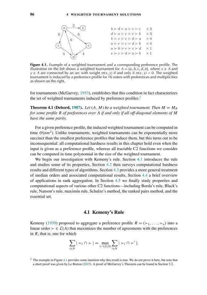
86 4 weighted tournament solutions
a b
c
d
e
2
6
4
6
6
4
b � d � a � e � c × 3
d � a � c � e � b × 3
b � c � e � d � a × 4
a � e � c � d � b × 4
a � b � c � e � d × 1
e � c � d � a � b × 1
Figure 4.1. Example of a weighted tournament and a corresponding preference profile. Theillustration on the left shows a weighted tournament for A = {a, b, c, d, e}, where x ∈ A andy ∈ A are connected by an arc with weight m(x, y) if and only if m(x, y) > 0. The weightedtournament is induced by a preference profile for 16 voters with preferences and multiplicitiesas shown on the right.
for tournaments (McGarvey, 1953), establishes that this condition in fact characterizesthe set of weighted tournaments induced by preference profiles.2
Theorem 4.1 (Debord, 1987). Let (A, M) be a weighted tournament. Then M = MR
for some profile R of preferences over A if and only if all off-diagonal elements of M
have the same parity.
For a given preference profile, the induced weighted tournament can be computed intime O(nm2). Unlike tournaments, weighted tournaments can be exponentially moresuccinct than the smallest preference profiles that induce them, but this turns out to beinconsequential: all computational hardness results in this chapter hold even when theinput is given as a preference profile, whereas all tractable C2 functions we considercan be computed in time polynomial in the size of the weighted tournament.
We begin our investigation with Kemeny’s rule. Section 4.1 introduces the ruleand studies some of its properties, Section 4.2 then surveys computational hardnessresults and different types of algorithms. Section 4.3 provides a more general treatmentof median orders and associated computational results, Section 4.4 a brief overviewof applications in rank aggregation. In Section 4.5 we finally study properties andcomputational aspects of various other C2 functions—including Borda’s rule, Black’srule, Nanson’s rule, maximin rule, Schulze’s method, the ranked pairs method, and theessential set.
4.1 Kemeny’s Rule
Kemeny (1959) proposed to aggregate a preference profile R = (�1, . . . ,�n) into alinear order � ∈ L(A) that maximizes the number of agreements with the preferencesin R, that is, one for which∑
i∈N
| �i ∩ � | = max�′∈L(A)
∑i∈N
| �i ∩ �′ |.
2 The example in Figure 4.1 provides some intuition why this result is true. We do not prove it here, but note thata short proof was given by Le Breton (2005). A proof of McGarvey’s Theorem can be found in Section 3.2.

4 .1 kemeny’s rule 87
Orders with this property are an example of so-called median orders (Barthelemy andMonjardet, 1981; Charon and Hudry, 2007), which will be discussed more generallyin Section 4.3. The social preference function that selects all such orders is the onlyneutral and consistent Condorcet extension (Young and Levenglick, 1978) and hasalso been characterized as the maximum likelihood estimator for a simple probabilisticmodel in which individual preferences are noisy estimates of an underlying “true”ranking (Young, 1988, 1995a).3 We will see momentarily that Kemeny’s rule is veryinteresting also from a computational perspective, and will devote a significant part ofthis chapter to its study.
In the literature, Kemeny’s rule is often defined by minimization of disagreementrather than maximization of agreement. To this end, define the (Kemeny) score of aranking � with respect to a preference profile R = (�1, . . . ,�n) as∑
i∈N
τ (�i ,�),
where
τ (�i ,�) =∑
{x,y}⊆A
dx,y(�i ,�)
with
dx,y(�i ,�) ={
1 if x �i y and y � x, or y �i x and x � y
0 otherwise
is Kendall’s tau distance (Kendall, 1938). In other words, the score of � measuresthe sum of distances to the individual preference orders �i in terms of the number ofinversions. Kemeny’s rule then chooses rankings with minimum score.4 Because
∑i∈N
τ (�i ,�) =∑
x,y∈A
x�y
∣∣{i ∈ N : y �i x}∣∣ =∑x,y∈A
x�y
mR(y, x) + n
2,
Kemeny’s rule is a C2 function. This characterization also emphasizes the close rela-tionship between Kemeny’s rule and Slater’s rule (Chapter 3), which only takes the signof each majority margin into account when computing scores and ignores its absolutevalue.
We leave it to the reader to verify that in the example of Figure 4.1 alternative a isthe unique Kemeny winner, that is, the unique alternative at the top of a ranking withminimum score.
3 Quite surprisingly, the alternative most likely to be the best may not simply be the alternative at the top of theranking with the highest likelihood. In fact Borda’s rule, which we discuss in Section 4.5.1, may provide a betterestimate in this case (Young, 1988).
4 There can in fact be up to m! such rankings. It is also worth noting that other social choice functions can beobtained by maximizing score over a set of rankings other than linear orders, see Section 4.3 for details.
88 4 weighted tournament solutions
4.2 Computing Kemeny Winners and Kemeny Rankings
We consider three decision problems and one optimization problem related to Kemeny’srule.
Kemeny ScoreInput: A preference profile R and a nonnegative integer k.Question: Is there a linear order that has score at most k with respect to R?
Kemeny WinnerInput: A preference profile R and an alternative x ∈ A.Question: Is there a linear order that has minimum score with respect to R and ranks x
first?
Kemeny RankingInput: A preference profile R and two alternatives x, y ∈ A.Question: Is there a linear order that has minimum score with respect to R and ranks
x above y?
Kemeny Rank AggregationInput: A preference profile R.Task: Find a linear order that has minimum score with respect to R.
We will see that the first decision problem is NP-complete, whereas the other twoseem computationally even harder: they are complete for the class �P
2 of problemssolvable via parallel access to NP.5 From a practical point of view, Kemeny RankAggregation is perhaps most interesting.
We begin with a discussion of the classical completeness results mentioned above,and then we explore two approaches that attempt to address the computationalintractability these completeness results imply: exponential-time parameterized algo-rithms, and polynomial-time approximation algorithms for Kemeny Rank Aggre-gation. Finally we discuss additional approaches—exact, approximate, or purelyheuristic—that are relevant in practice.
4.2.1 Computational Hardness
If there are only two voters, the preference order of either of them has minimumKemeny score. By contrast, it was known since the late 1980s that Kemeny Scoreis NP-complete when the number n of voters is unbounded (Bartholdi et al., 1989a;Hudry, 1989). This result was later shown to hold already for n = 4, and in fact forany even n � 4. Quite intriguingly, the case for any odd n � 3 remains open.
Theorem 4.2 (Bartholdi et al., 1989b; Hudry, 1989; Dwork et al., 2001; Biedlet al., 2009). Kemeny Score is NP-complete for even n � 4, and for odd n when n isunbounded.
5 A detailed discussion of this complexity class, and related results for Dodgson’s and Young’s rules, can befound in Chapter 5.
4 .2 computing kemeny winners and kemeny rankings 89
Proof sketch. The Kemeny score of a given linear order can easily be computed andcompared to k in polynomial time, so Kemeny Score is in NP.
Hardness for the two cases can be shown by two polynomial-time reductions fromthe NP-complete feedback arc set problem on directed graphs (e.g., Garey and Johnson,1979), here we sketch the reduction for even n � 4.
Feedback Arc SetInput: A directed graph G = (V, E) and an integer k � 0.Question: Is there a set F ⊆ E with |F | � k such that graph G′ = (V, E \ F ) does
not have any directed cycles?
Consider a directed graph G = (V, E) with V = {v1, . . . , vn} and an integer k � 0,and let m = |E|. The goal is to find in polynomial time a preference profile R and aninteger k′ such that there exist a linear order that has Kemeny score at most k′ withrespect to R if and only if G has a feedback arc set of size at most k. To this end,let A = V ∪ E. For each v ∈ V , let out(v) and in(v) respectively denote arbitrary linearorders of the incoming and outgoing arcs of v. For any linear order �, let � denote thereverse order. Now define R as the set of the following four linear orders, where weslightly abuse notation and compose linear orders from linear orders on subsets of thealternatives:
v1 �1 out(v1) �1 v2 �1 out(v2) �1 . . . �1 vn �1 out(vn),
vn �2 out(vn) �2 vn−1 �2 out(vn−1) �2 . . . �2 v1 �2 out(v1),
in(v1) �3 v1 �3 in(v2) �3 v2 �3 . . . �3 in(vn) �3 vn,
in(vn) �4 vn �4 in(vn−1) �4 vn−1 �4 . . . �4 in(v1) �4 v1.
Setting k′ = 2(n2
)+ 2(m2
)+ 2m(n − 1) + 2k completes the construction.For a rigorous proof of correctness, the reader is referred to the article of Biedl et al.
(2009). It is not hard to show, however, that independently of the structure of graph G
any linear order of A must have score at least k′ − 2k with respect to R. Given afeedback arc set F of size k, a linear order on A \ F that has score k′ − 2k with respectto the restriction of R to A \ F can be obtained by starting from a topological orderingof the acyclic graph (V, E \ F ) and inserting each arc (u, v) ∈ E \ F between u and v.Inserting each arc (u, v) ∈ F immediately after u, as in �1 and �2, increases the scoreby 2k due to �3 and �4, for an overall score of k′.
The result can easily be generalized to any even number n � 6 of voters by adding(n − 4)/2 voters with an arbitrary preference order and (n − 4)/2 voters with thereverse preference order.
While NP-hardness of Kemeny Winner and Kemeny Ranking follow from The-orem 4.2 and were thus known since 1989, the exact complexity of these problemsremained open until they were finally shown complete for the class �P
2 of problemsthat can be decided by parallel access to an oracle for NP. Membership in �P
2 isstraightforward. The proof of hardness follows the same general idea as the proof ofBartholdi et al. (1989b) for NP-hardness of Kemeny Score, but starts from a �P
2 -complete variant of Feedback Arc Set, referred to as Feedback Arc Set Member,
90 4 weighted tournament solutions
and reduces this problem in polynomial time to both Kemeny Winner and KemenyRanking.
Theorem 4.3 (Hemaspaandra et al., 2005). Kemeny Winner and Kemeny Rank-ing are �P
2 -complete.
The usual interpretation of the above results is that general efficient algorithms forKemeny’s rule are unlikely to exist, where efficiency is associated with running timesthat are polynomial in the size of the problem instance. We proceed to discuss differentalgorithmic approaches by which this difficulty can be and has been addressed. Wefocus mainly on Kemeny Rank Aggregation, but note that most of the techniquescan easily be adapted to the three decision problems.
4.2.2 Polynomial-Time Approximation Algorithms
A common approach to computationally difficult problems sacrifices solution quality toachieve a polynomial running time, while trying to guarantee that the solution remainsclose to optimal. To this end, call an algorithm a polynomial-time α-approximationalgorithm for Kemeny Rank Aggregation if it has polynomial running time and foreach preference profile produces a linear order with Kemeny score at most α times theminimum Kemeny score.
Ordering the alternatives by increasing Borda score provides a 5-approximation toKemeny Rank Aggregation (Coppersmith et al., 2010). Because τ is a metric andin particular satisfies the triangle inequality, the preference order of a voter selecteduniformly at random in fact yields a 2-approximation in expectation, and this argumentcan easily be de-randomized to obtain a deterministic polynomial-time algorithm withthe same approximation factor (e.g., Ailon et al., 2008). Spearman’s footrule distance,that is, the sum of the absolute values of the difference between ranks, providesanother polynomial-time 2-approximation algorithm (Diaconis and Graham, 1977;Dwork et al., 2001), and it turns out that the approximation factor can be improvedfurther.
Theorem 4.4 (Ailon et al., 2008; van Zuylen and Williamson, 2009). The followingpolynomial-time algorithms exist for Kemeny Rank Aggregation:
� a 4/3-approximation algorithm based on linear programming;� a combinatorial 11/7-approximation algorithm.
The 11/7-approximation algorithm selects the better of two linear orders: the pref-erence order of a voter chosen uniformly at random and the order obtained by analgorithm similar to quicksort, which chooses a pivot alternative and recursively ordersthe alternatives above and below that alternative (Ailon et al., 2008). The approxima-tion guarantee can be improved to 4/3 if the pivot element is chosen randomly basedon the solution of a linear program (Ailon et al., 2008), and this algorithm can be de-randomized while preserving the approximation factor (van Zuylen and Williamson,2009).
Whereas all of the above algorithms are reasonably efficient also in practice, thefollowing result is of purely theoretical interest.

4 .2 computing kemeny winners and kemeny rankings 91
Theorem 4.5 (Kenyon-Mathieu and Schudy, 2007). Kemeny Rank Aggregationhas an efficient polynomial-time approximation scheme.
An efficient polynomial-time approximation scheme computes an (1 + ε)-approximation in polynomial time for any ε > 0, where the degree of the polynomialis independent of ε but the running time can otherwise depend on ε in an arbitraryway. The running time of the algorithm underlying Theorem 4.5 is doubly exponentialin 1/ε, which is too large for most practical purposes. Theorem 4.5 does imply, how-ever, that no constant lower bound greater than one exists on possible approximationfactors for Kemeny Rank Aggregation, so there is hope that Theorem 4.4 can beimproved upon by algorithms that are efficient in practice.
4.2.3 Parameterized Algorithms
Parameterized algorithms provide a different approach to computationally difficultproblems, by attempting to limit any super-polynomial growth of the running time tocertain parameters of the problem at hand. If the attempt is successful the problemis fixed-parameter tractable, that is, it can be solved efficiently for small parametervalues (e.g., Downey and Fellows, 2013; Niedermeier, 2006).
Perhaps the most obvious candidate parameters in our setting are the number n
of voters and the number m of alternatives. Whereas a restriction of n makes littlesense given the NP-completeness of Kemeny Score for n = 4, the situation looksmore promising for m. Indeed, an exhaustive search through all possible linear ordersfor one with minimum score requires O(m! nm log m) time, where O(nm log m) isthe time needed to compute the score of a single linear order. While this algo-rithm could be used to solve instances with around ten alternatives, the excessivegrowth of m! limits its usefulness. Dynamic programming enables a reduction of thisfactor to 2m.
Theorem 4.6 (Betzler et al., 2009; Raman and Saurabh, 2007). Kemeny RankAggregation can be solved in O(2mm2n) time.
Proof sketch. Consider a preference profile R on a set A of alternatives. We inductivelycompute a Kemeny ranking for the restriction of R to every nonempty subset of A.For subsets of size one, computation of a Kemeny ranking is trivial. For A′ ⊆ A with|A′| > 1, we exploit the fact that the exclusion of the alternative at the top of a Kemenyranking does not change the relative ranking of the other alternatives (e.g., Young,1988). A Kemeny ranking for A′ can thus be found by considering all linear orders thatbegin with some alternative a ∈ A′ and continue with a Kemeny ranking for A′ \ {a}.There are |A′| � m such rankings, and the score of each such ranking can be computedfrom that of a Kemeny ranking for A′ \ {a} in O(nm) time. Because the algorithmconsiders each nonempty subset of A, its running time is O(2mm2n).
Another obvious class of parameters includes the Kemeny score of the instance athand, which we denote by k in the following, the average distance τavg between pref-erence orders, and the average distance between the preference orders and a Kemenyranking, which is equal to k/n. Simjour (2009) observed that k/(n − 1) � τavg � 4k/n,which makes k/n a stronger parameter than τavg in the sense that it takes smaller
92 4 weighted tournament solutions
values (Komusiewicz and Niedermeier, 2012). The advantage of τavg is that it caneasily be computed for a given preference profile. In the following we state resultsin terms of k/n, but they clearly hold for τavg and any other upper bound on k/n aswell.
The main theoretical result for this type of parameterization is a sub-exponentialalgorithm that makes use of a standard reduction from Kemeny Score to WeightedFeedback Arc Set in tournaments and a dynamic programming algorithm for thelatter.
Theorem 4.7 (Karpinski and Schudy, 2010). Kemeny Rank Aggregation can besolved in 2O(
√k/n) + (n + m)O(1) time.
Fomin et al. (2010) gave a sub-exponential algorithm for a local search variant ofKemeny Rank Aggregation. Mahajan et al. (2009) showed that Kemeny Scoreremains fixed-parameter tractable if instead of k it is parameterized by the differencebetween k and a certain lower bound on the Kemeny score that can be shown to holdfor a given preference profile.
Parameterization in terms of k and related parameters also enables a more detailedanalysis of preprocessing techniques. Even when the existence of polynomial-timealgorithms for a certain problem is unlikely, we may still hope for polynomial-timedata reduction rules that provably reduce the size of the input instance (Guo andNiedermeier, 2007). Knowledge of k can for example be used to reduce the numberof voters to at most 2k, by distinguishing instances where at most k and more than k
voters have the same preference order. In the former case, any instance with more than2k voters would have Kemeny score greater than k. In the latter case, the preferenceorder shared by more than k voters is the only one that can have score k or less andmust thus be a Kemeny ranking.
Two additional data reduction rules can be obtained from an extension of the Con-dorcet criterion (Truchon, 1998). A linear order � ∈ L(A) satisfies the extended Con-dorcet criterion with respect to a preference profile R on A if the following holds: ifthere exists A′ ⊆ A such that mR(x, y) > 0 for all x ∈ A′ and y ∈ A \ A′, then x � y
for all x ∈ A′ and y ∈ A \ A′.
Lemma 4.8 (Truchon, 1998). Any Kemeny ranking satisfies the extended Condorcetcriterion.
This lemma implies, for example, that an alternative that is ranked in the sameway by all voters relative to all other alternatives must appear in a fixed position inevery Kemeny ranking. More interestingly, the lemma suggests a recursive way ofcomputing a Kemeny ranking that can be applied whenever some set A′ ⊆ A satisfiesthe condition of the extended Condorcet criterion. In this case the elements of A′ mustbe ranked above the elements of A \ A′, and the restrictions of the Kemeny ranking toA′ and A \ A′ must be Kemeny rankings of the respective restrictions of the preferenceprofile.
These insights can be combined with an exhaustive search for Kemeny rankings ofat most 2/ε alternatives, for some ε > 0, and with a connection to a weighted versionof Feedback Arc Set, to obtain the following result.
4 .2 computing kemeny winners and kemeny rankings 93
Theorem 4.9 (Simjour, 2013). For any ε > 0, a given preference profile can betransformed in polynomial time into a preference profile with at most (2 + ε)k/n
alternatives that is equivalent with regard to Kemeny Rank Aggregation.
Other parameters that have been considered in the literature include the positionseach alternative takes in the preferences of individual voters, and the distance to single-peaked or single-crossing preferences.
For a given preference profile, define the range of an alternative as one plus thedifference between the highest and the lowest rank this alternative takes in the prefer-ence order of any voter. Let rmax denote the maximum range of any alternative and ravg
the average range of the alternatives. It is now not difficult to see that Kemeny RankAggregation remains NP-hard even for preference profiles with ravg = 2. For this,consider an arbitrary preference profile and add m2 new alternatives that are rankedbelow the original alternatives and in the same relative order in all preference orders.Then, any Kemeny ranking with respect to the new preference profile ranks the orig-inal alternatives above the new ones, and its restriction to the original alternatives isa Kemeny ranking with respect to the original preference profile. Moreover, the newprofile has an average range of at most 2. By contrast, Kemeny Rank Aggregationcan be solved in O(32rmax (r2
max + rmaxm2)) time using dynamic programming (Betzler
et al., 2009).Cornaz et al. (2013) obtained a characterization in terms of the single-peaked or
single-crossing width of a preference profile, which respectively measure its distance toa single-peaked or single-crossing profile. Here, a preference profile is single-peaked ifthere exists a linear order of the alternatives such that each voter prefers alternatives lessif they are further away in this order from its most preferred alternative. A preferenceprofile is single-crossing if there exists a linear order of the voters such that for anytwo alternatives x and y the voters preferring x over y are ranked above the voterspreferring y over x, or vice versa.
4.2.4 Practical Algorithms
All of the algorithms we have discussed so far come with some kind of formal guaranteeregarding their running time or the quality of solutions they produce. These guaranteeshold in the worst case over all preference profiles or over a restricted set of profiles withcertain parameters. It is, however, not obvious that the algorithms with the strongestworst-case guarantees are the best algorithms in practice. A fair amount of work hastherefore been done to validate them empirically, and potentially identify algorithmsthat perform better on realistic problem instances. We provide a brief overview, andrefer the interested reader to the individual articles and to the survey of Charon andHudry (2010) for details.
In discussing the empirical work, it again makes sense to distinguish two classes ofalgorithms: exact algorithms that are guaranteed to produce an optimal ranking, andwhere the goal is to reduce the running time to a reasonable level; and suboptimalalgorithms that provide a trade-off between solution quality and running time and thatmay come with or without formal guarantees for either of these two characteristics.

94 4 weighted tournament solutions
Both classes of algorithms may use heuristics designed to reduce running time orimprove solution quality in practice.
Members of the former class that have been evaluated include algorithms based oninteger linear programming, branch and cut, and branch and bound (Davenport andKalagnanam, 2004; Conitzer et al., 2006; Charon and Hudry, 2006; Schalekamp andvan Zuylen, 2009; Ali and Meila, 2012). In addition, effectiveness of the data reductionrules of Section 4.2.3 has been confirmed empirically (Betzler et al., 2014). While thedynamic programming algorithm underlying Theorem 4.6 is competitive only for verysmall numbers of alternatives, a combination of integer programming with polynomial-time data reduction and other techniques for reducing the running time leads to thefastest known algorithms in all other cases.
The second class of algorithms provides an even wider range of options. Here,Schalekamp and van Zuylen (2009) recommend a heuristic based on Borda scoreswhen the goal is to obtain reasonably good results very quickly, and an algorithmbased on Copeland’s method for higher solution quality and slightly larger runningtime. At the cost of a further increase in running time, an initial solution may beimproved further using local search. The analysis of Schalekamp and van Zuylenwas extended by Ali and Meila (2012), who investigated how the structure of pref-erence profiles affects the complexity of finding a Kemeny ranking, and how thisinformation can be used to select an appropriate algorithm. This approach is similarto parameterized complexity analysis in that it tries to identify certain structures in theproblem input that enable faster algorithms, but at the same time abandons exactnessof solutions and worst-case bounds on the running time in favor of improved practicalperformance.
It is finally worth mentioning that a rich set of metaheuristics has been applied toKemeny’s rule, including simulated annealing, tabu search, and genetic algorithms.The interested reader is again referred to the survey of Charon and Hudry (2010).
4.3 Further Median Orders
Kemeny’s rule is defined in terms of linear orders that maximize the number of agree-ments with a given set of linear orders. The central role of linear orders in social choicetheory notwithstanding, one may also more generally consider the problem of findinga binary relation from a set M that maximizes the number of agreements with a setof binary relations taken from a set V . We focus here on sets M and V obtainedby relaxing some of the properties that characterize linear orders—completeness,transitivity, and asymmetry—and refer to the literature for additional properties(Barthelemy and Monjardet, 1981; Fishburn, 1985; Bouyssou et al., 2006; Caspardet al., 2012) and complexity results (Wakabayashi, 1998; Hudry, 2008; Charon andHudry, 2010).
For a set A of alternatives, let B(A) denote the set of (binary) relations, T (A) theset of complete and asymmetric relations, and R(A) the set of complete and tran-sitive relations on A. Obviously, T (A) is the set of tournaments on A. Relationsin R(A), which are also called weak orders, can model indifferences or incomparabil-ities among alternatives, but not both. Note also that for any A, L(A) ⊆ T (A) ⊆ B(A)

4 .3 further median orders 95
and L(A) ⊆ R(A) ⊆ B(A). We now consider the following decision problem forM,V ∈ {B,R, T ,L}.6
(V,M)-ScoreInput: An element of V(A)n and a nonnegative integer k.Question: Is there an element of M(A) with score at most k?
By Theorem 4.2 (L,L)-Score, or Kemeny Score, is NP-complete for any evennumber of voters greater than or equal to four and for an unbounded odd number ofvoters.7 It is easy to see that membership in NP holds for all of the preceding choicesof M and V . Because NP-hardness is established by identifying certain elements of Vfor which the existence of an element of M(A) with score at most k is hard to decide,it continues to hold if elements are added to V . This means in particular that (V,L)-Score is NP-complete for any V ⊇ L. Taking V to be a strict superset of L could ofcourse render the problem more difficult, and indeed (T ,L)-Score is hard even for asingle voter.
Theorem 4.10 (Alon, 2006; Charbit et al., 2007; Conitzer, 2006). (T ,L)-Score isNP-complete, even when n = 1.
The attentive reader may have recognized the single-voter variant as a subproblemin the computation of the Slater set of Chapter 3, and Theorem 3.3 is in fact a corollaryof Theorem 4.10.
The dependence of the complexity of (V,M)-Score on M is less obvious, but wewill see that hardness can in many cases be attributed to transitivity. Wakabayashi (1986,1998) studied (B,M)-Score for various choices of M, and identified transitivity ofthe relations in M as a source of hardness. NP-completeness for M = L can beobtained as a corollary of Theorem 4.2, but the problem remains NP-complete whencompleteness, asymmetry, or both are relaxed. If we instead relax transitivity and keepcompleteness, asymmetry, or both, the problem can be solved in polynomial time.
Theorem 4.11 (Wakabayashi, 1986, 1998). (B,R)-Score is NP-complete. (B, T )-Score can be solved in polynomial time.
Theorems 4.2 and 4.10 can respectively be extended to (L,R)-Score and (T ,R)-Score, which by earlier arguments also strengthens the first part of Theorem 4.11.
Theorem 4.12 (Hudry, 2012). (L,R)-Score is NP-complete for every even n � 4.(T ,R)-Score is NP-complete, even when n = 1.
6 In the context of this problem the term complete preorders has sometimes been used incorrectly for all elementsof R and not just those that satisfy reflexivity. It is, however, easy to see that the addition of reflexivity orirreflexivity to V or M does not affect the relative sizes of scores or the complexity of (V,M)-Score, so thatall statements concerning R in what follows hold also for complete pre-orders. Also in what follows, statementsconcerning linear orders remain true, sometimes nontrivially, if linearity is replaced by acyclicity. We leave itto the interested reader to verify that this is indeed the case.
7 Kemeny (1959) in fact followed Arrow (1951) in requiring only completeness and transitivity, and considered(R,R)-Score. We will obtain a hardness result concerning (R,R)-Score toward the end of this section.
96 4 weighted tournament solutions
Ignoring the dependence on the number of voters, and denoting by A(A) the set ofacyclic relations on A, sufficient conditions for NP-completeness can be summarizedas follows.
Theorem 4.13. (V,M)-Score is NP-complete if V ⊇ L and M ∈ {A,R,L}.
4.4 Applications in Rank Aggregation
The enormous interest in Kemeny’s rule and other median orders across various dis-ciplines can to a certain extent be attributed to its importance in rank aggregation,with applications that extend far beyond the realm of social choice. Rank aggregationproblems arise for instance in the context of planning in multiagent systems (e.g.,Ephrati and Rosenschein, 1993), in the design of metasearch engines and in spamdetection (e.g., Cohen et al., 1999; Dwork et al., 2001), in collaborative filteringand recommender systems (e.g., Pennock et al., 2000a), in computational biology(e.g., Jackson et al., 2008), and in winner determination for sports competitions (e.g.,Betzler et al., 2014). Here we briefly describe an application to similarity search andclassification for high-dimensional data (Fagin et al., 2003).
Assume we are given a set of n data points and an additional query point, both froma Euclidean space, and are interested in finding data points that are similar to the querypoint. This problem can be reduced to a rank aggregation problem by associating eachdata point with an alternative, and each dimension with a voter who ranks alternatives inincreasing distance from the query point in that dimension. What makes this approachparticularly attractive in the context of databases is that it does not require complex datastructures or a large amount of additional storage and mostly avoids random access tothe data. It of course relies on an efficient algorithm for rank aggregation, and Faginet al. (2003) specifically propose an approximate solution using the footrule distance.
4.5 Other C2 Functions
Whereas a large part of the computational work on C2 functions has focused onKemeny’s rule and other median orders, classical social choice theory has studiedvarious other C2 functions, mostly with regard to their relationships and axiomaticproperties.
4.5.1 Variations of Borda’s Rule
The first class of functions we consider are variations of a well-known choice ruledue to Borda (1781). Borda’s rule is commonly defined as the scoring rule with scorevector s = (m − 1, m − 2, . . . , 0). Under a scoring rule, an alternative receives score sj
whenever some voter ranks it in position j . These scores are then added up for all voters,and the alternatives with maximum cumulative score are selected (also see Section 2.4).Borda’s rule in particular can be viewed as selecting the alternatives with the highestaverage rank in the individual preferences. Interestingly, the Borda score of alternative
4 .5 other c2 functions 97
x is equal to∑i∈N
|{y ∈ A : x �i y}| =∑y∈A
|{i ∈ N : x �i y}| =∑y∈A
m(x, y) + n
2
and thus only depends on the majority margins. Borda’s rule fails the Condorcetcriterion,8 but this is easily fixed. Black’s rule selects a Condorcet winner if it exists,and the alternatives with maximum Borda score otherwise (Black, 1958). Nanson’s rulesuccessively excludes the alternatives whose Borda scores are below the average untilall remaining alternatives have the same Borda score (Nanson, 1882). It is a Condorcetextension because the Borda score of a Condorcet winner is always at least the averageBorda score. In the example of Figure 4.1, the unique alternative selected by each ofthese C2 functions is alternative a.
It is easy to see that the complexity of Borda’s, Black’s, and Nanson’s rules isdominated by that of the Borda scores, which can be computed from the majoritymargins in time O(m2). The same is true for the choice rule obtained by successiveexclusion of all alternatives with minimum Borda score, which is sometimes attributedto Nanson but differs from Nanson’s rule (see Niou, 1987).
4.5.2 Maximin Rule and Schulze’s Method
Maximin rule (Young, 1977), also known as Condorcet’s rule or the Simpson-Kramermethod, selects alternatives for which the minimum pairwise majority margin is max-imized, that is, alternatives x for which
minz∈A
m(x, z) = maxy∈A
minz∈A
m(y, z).
Such an alternative is desirable in the sense that it minimizes the number of overruledvoters, and can be computed from the majority margins in time O(m2). A drawbackof maximin rule is that it violates a number of desirable properties, most notablythe Condorcet loser criterion. A Condorcet loser for a given preference profile is analternative to which every other alternative is preferred by a majority of the voters, andthe Condorcet loser criterion requires that a Condorcet loser can never be selected.9
Another C2 function, closer to Borda’s rule but still violating the criterion, can beobtained by selecting alternatives that maximize the sum rather than the minimum oftheir majority margins with negative sign (Tideman, 2006, p. 199). This function willbe discussed in a different context in Section 5.6.2.
8 Borda’s rule does, however, maximize the probability of selecting a Condorcet winner among all scoring rulesfor a preference profile chosen uniformly at random from the set of all preference profiles, in the limit as thenumber of voters goes to infinity (Gehrlein and Fishburn, 1978). While Borda’s rule and Kemeny’s rule mayproduce very different outcomes, both rules agree in the relative ranking of their respective best and worstalternatives (Saari and Merlin, 2000): for any Kemeny ranking, the top alternative has a higher Borda scorethan the bottom alternative; conversely, Kemeny’s rule ranks an alternative with maximum Borda score abovean alternative with minimum Borda score.
9 In the example of Figure 4.1, maximin rule selects an alternative not preferred to any other alternative by amajority of the voters. It is easy to extend this example to a violation of the Condorcet loser criterion, showingthat most other social choice functions satisfy the criterion is a more substantial exercise.
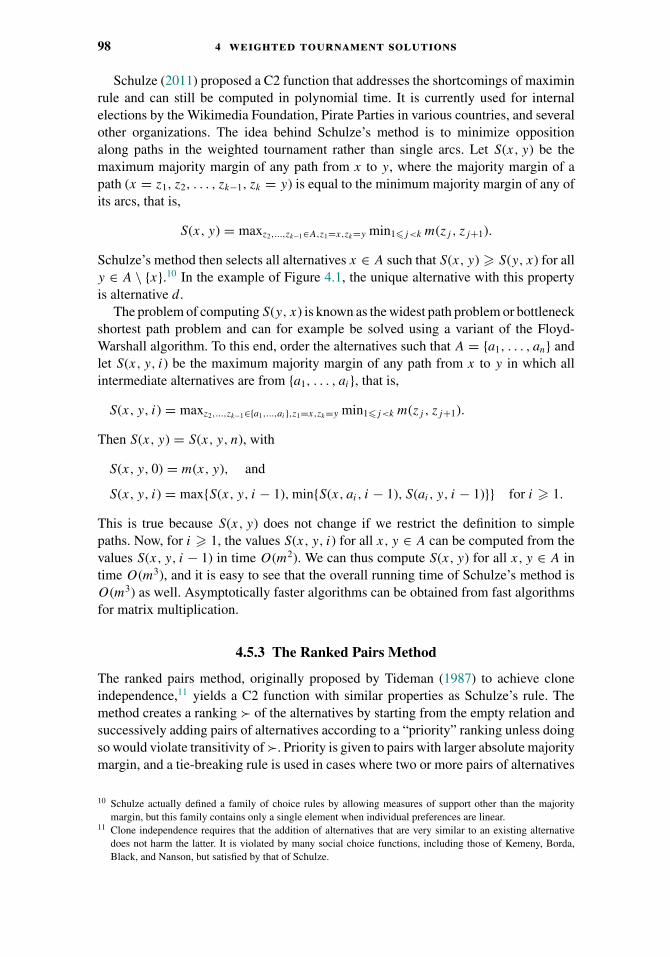
98 4 weighted tournament solutions
Schulze (2011) proposed a C2 function that addresses the shortcomings of maximinrule and can still be computed in polynomial time. It is currently used for internalelections by the Wikimedia Foundation, Pirate Parties in various countries, and severalother organizations. The idea behind Schulze’s method is to minimize oppositionalong paths in the weighted tournament rather than single arcs. Let S(x, y) be themaximum majority margin of any path from x to y, where the majority margin of apath (x = z1, z2, . . . , zk−1, zk = y) is equal to the minimum majority margin of any ofits arcs, that is,
S(x, y) = maxz2,...,zk−1∈A,z1=x,zk=y min1�j<k m(zj , zj+1).
Schulze’s method then selects all alternatives x ∈ A such that S(x, y) � S(y, x) for ally ∈ A \ {x}.10 In the example of Figure 4.1, the unique alternative with this propertyis alternative d.
The problem of computing S(y, x) is known as the widest path problem or bottleneckshortest path problem and can for example be solved using a variant of the Floyd-Warshall algorithm. To this end, order the alternatives such that A = {a1, . . . , an} andlet S(x, y, i) be the maximum majority margin of any path from x to y in which allintermediate alternatives are from {a1, . . . , ai}, that is,
S(x, y, i) = maxz2,...,zk−1∈{a1,...,ai},z1=x,zk=y min1�j<k m(zj , zj+1).
Then S(x, y) = S(x, y, n), with
S(x, y, 0) = m(x, y), and
S(x, y, i) = max{S(x, y, i − 1), min{S(x, ai, i − 1), S(ai, y, i − 1)}} for i � 1.
This is true because S(x, y) does not change if we restrict the definition to simplepaths. Now, for i � 1, the values S(x, y, i) for all x, y ∈ A can be computed from thevalues S(x, y, i − 1) in time O(m2). We can thus compute S(x, y) for all x, y ∈ A intime O(m3), and it is easy to see that the overall running time of Schulze’s method isO(m3) as well. Asymptotically faster algorithms can be obtained from fast algorithmsfor matrix multiplication.
4.5.3 The Ranked Pairs Method
The ranked pairs method, originally proposed by Tideman (1987) to achieve cloneindependence,11 yields a C2 function with similar properties as Schulze’s rule. Themethod creates a ranking � of the alternatives by starting from the empty relation andsuccessively adding pairs of alternatives according to a “priority” ranking unless doingso would violate transitivity of �. Priority is given to pairs with larger absolute majoritymargin, and a tie-breaking rule is used in cases where two or more pairs of alternatives
10 Schulze actually defined a family of choice rules by allowing measures of support other than the majoritymargin, but this family contains only a single element when individual preferences are linear.
11 Clone independence requires that the addition of alternatives that are very similar to an existing alternativedoes not harm the latter. It is violated by many social choice functions, including those of Kemeny, Borda,Black, and Nanson, but satisfied by that of Schulze.
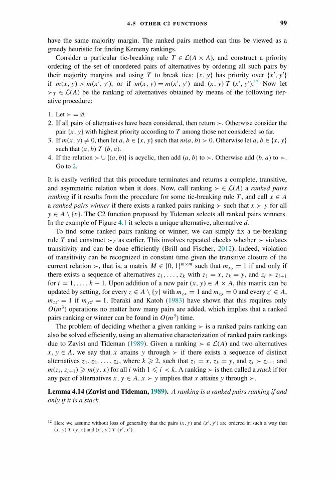
4 .5 other c2 functions 99
have the same majority margin. The ranked pairs method can thus be viewed as agreedy heuristic for finding Kemeny rankings.
Consider a particular tie-breaking rule T ∈ L(A × A), and construct a priorityordering of the set of unordered pairs of alternatives by ordering all such pairs bytheir majority margins and using T to break ties: {x, y} has priority over {x ′, y ′}if m(x, y) > m(x ′, y ′), or if m(x, y) = m(x ′, y ′) and (x, y) T (x ′, y ′).12 Now let�T ∈ L(A) be the ranking of alternatives obtained by means of the following iter-ative procedure:
1. Let � = ∅.2. If all pairs of alternatives have been considered, then return �. Otherwise consider the
pair {x, y} with highest priority according to T among those not considered so far.3. If m(x, y) �= 0, then let a, b ∈ {x, y} such that m(a, b) > 0. Otherwise let a, b ∈ {x, y}
such that (a, b) T (b, a).4. If the relation � ∪ {(a, b)} is acyclic, then add (a, b) to �. Otherwise add (b, a) to �.
Go to 2.
It is easily verified that this procedure terminates and returns a complete, transitive,and asymmetric relation when it does. Now, call ranking � ∈ L(A) a ranked pairsranking if it results from the procedure for some tie-breaking rule T , and call x ∈ A
a ranked pairs winner if there exists a ranked pairs ranking � such that x � y for ally ∈ A \ {x}. The C2 function proposed by Tideman selects all ranked pairs winners.In the example of Figure 4.1 it selects a unique alternative, alternative d.
To find some ranked pairs ranking or winner, we can simply fix a tie-breakingrule T and construct �T as earlier. This involves repeated checks whether � violatestransitivity and can be done efficiently (Brill and Fischer, 2012). Indeed, violationof transitivity can be recognized in constant time given the transitive closure of thecurrent relation �, that is, a matrix M ∈ {0, 1}m×m such that mxy = 1 if and only ifthere exists a sequence of alternatives z1, . . . , zk with z1 = x, zk = y, and zi � zi+1
for i = 1, . . . , k − 1. Upon addition of a new pair (x, y) ∈ A × A, this matrix can beupdated by setting, for every z ∈ A \ {y} with mzx = 1 and mzy = 0 and every z′ ∈ A,mzz′ = 1 if myz′ = 1. Ibaraki and Katoh (1983) have shown that this requires onlyO(m3) operations no matter how many pairs are added, which implies that a rankedpairs ranking or winner can be found in O(m3) time.
The problem of deciding whether a given ranking � is a ranked pairs ranking canalso be solved efficiently, using an alternative characterization of ranked pairs rankingsdue to Zavist and Tideman (1989). Given a ranking � ∈ L(A) and two alternativesx, y ∈ A, we say that x attains y through � if there exists a sequence of distinctalternatives z1, z2, . . . , zk , where k � 2, such that z1 = x, zk = y, and zi � zi+1 andm(zi, zi+1) � m(y, x) for all i with 1 � i < k. A ranking � is then called a stack if forany pair of alternatives x, y ∈ A, x � y implies that x attains y through �.
Lemma 4.14 (Zavist and Tideman, 1989). A ranking is a ranked pairs ranking if andonly if it is a stack.
12 Here we assume without loss of generality that the pairs (x, y) and (x′, y′) are ordered in such a way that(x, y) T (y, x) and (x′, y′) T (y′, x′).
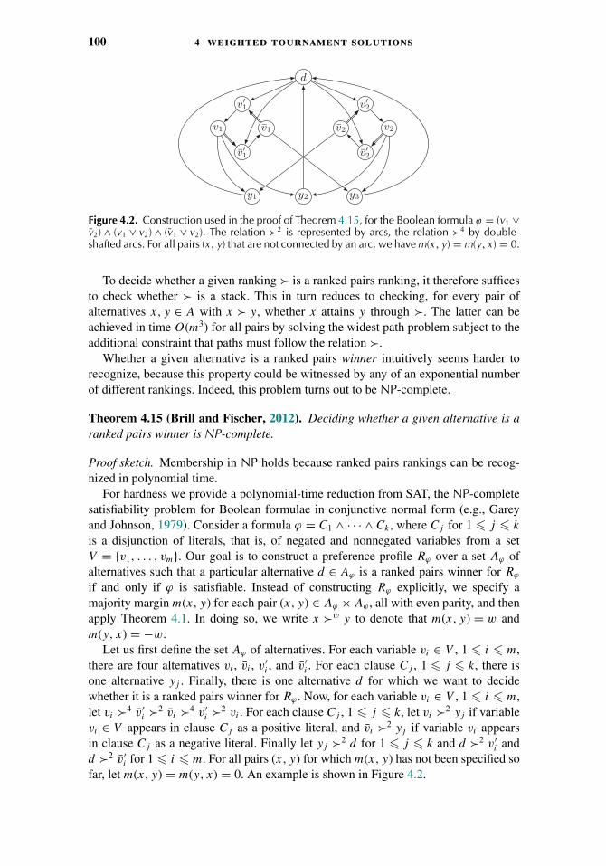
100 4 weighted tournament solutions
d
v1
v′1
v1
v′1
v2
v′2
v2
v′2
y1 y2 y3
Figure 4.2. Construction used in the proof of Theorem 4.15, for the Boolean formula ϕ = (v1 ∨v2) ∧ (v1 ∨ v2) ∧ (v1 ∨ v2). The relation �2 is represented by arcs, the relation �4 by double-shafted arcs. For all pairs (x, y) that are not connected by an arc, we have m(x, y) = m(y, x ) = 0.
To decide whether a given ranking � is a ranked pairs ranking, it therefore sufficesto check whether � is a stack. This in turn reduces to checking, for every pair ofalternatives x, y ∈ A with x � y, whether x attains y through �. The latter can beachieved in time O(m3) for all pairs by solving the widest path problem subject to theadditional constraint that paths must follow the relation �.
Whether a given alternative is a ranked pairs winner intuitively seems harder torecognize, because this property could be witnessed by any of an exponential numberof different rankings. Indeed, this problem turns out to be NP-complete.
Theorem 4.15 (Brill and Fischer, 2012). Deciding whether a given alternative is aranked pairs winner is NP-complete.
Proof sketch. Membership in NP holds because ranked pairs rankings can be recog-nized in polynomial time.
For hardness we provide a polynomial-time reduction from SAT, the NP-completesatisfiability problem for Boolean formulae in conjunctive normal form (e.g., Gareyand Johnson, 1979). Consider a formula ϕ = C1 ∧ · · · ∧ Ck , where Cj for 1 � j � k
is a disjunction of literals, that is, of negated and nonnegated variables from a setV = {v1, . . . , vm}. Our goal is to construct a preference profile Rϕ over a set Aϕ ofalternatives such that a particular alternative d ∈ Aϕ is a ranked pairs winner for Rϕ
if and only if ϕ is satisfiable. Instead of constructing Rϕ explicitly, we specify amajority margin m(x, y) for each pair (x, y) ∈ Aϕ × Aϕ , all with even parity, and thenapply Theorem 4.1. In doing so, we write x �w y to denote that m(x, y) = w andm(y, x) = −w.
Let us first define the set Aϕ of alternatives. For each variable vi ∈ V , 1 � i � m,there are four alternatives vi , vi , v′
i , and v′i . For each clause Cj , 1 � j � k, there is
one alternative yj . Finally, there is one alternative d for which we want to decidewhether it is a ranked pairs winner for Rϕ . Now, for each variable vi ∈ V , 1 � i � m,let vi �4 v′
i �2 vi �4 v′i �2 vi . For each clause Cj , 1 � j � k, let vi �2 yj if variable
vi ∈ V appears in clause Cj as a positive literal, and vi �2 yj if variable vi appearsin clause Cj as a negative literal. Finally let yj �2 d for 1 � j � k and d �2 v′
i andd �2 v′
i for 1 � i � m. For all pairs (x, y) for which m(x, y) has not been specified sofar, let m(x, y) = m(y, x) = 0. An example is shown in Figure 4.2.
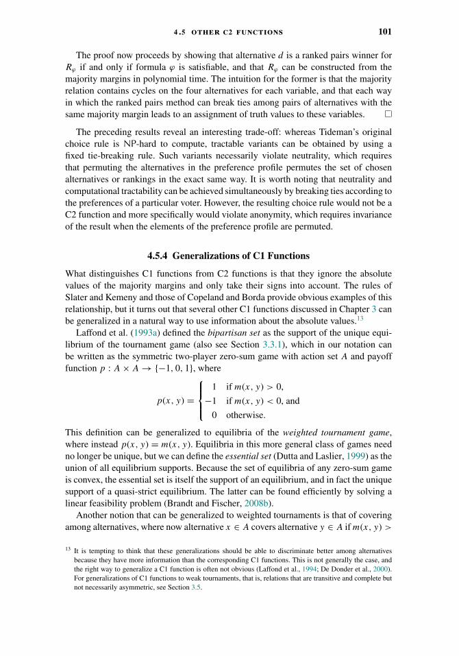
4 .5 other c2 functions 101
The proof now proceeds by showing that alternative d is a ranked pairs winner forRϕ if and only if formula ϕ is satisfiable, and that Rϕ can be constructed from themajority margins in polynomial time. The intuition for the former is that the majorityrelation contains cycles on the four alternatives for each variable, and that each wayin which the ranked pairs method can break ties among pairs of alternatives with thesame majority margin leads to an assignment of truth values to these variables.
The preceding results reveal an interesting trade-off: whereas Tideman’s originalchoice rule is NP-hard to compute, tractable variants can be obtained by using afixed tie-breaking rule. Such variants necessarily violate neutrality, which requiresthat permuting the alternatives in the preference profile permutes the set of chosenalternatives or rankings in the exact same way. It is worth noting that neutrality andcomputational tractability can be achieved simultaneously by breaking ties according tothe preferences of a particular voter. However, the resulting choice rule would not be aC2 function and more specifically would violate anonymity, which requires invarianceof the result when the elements of the preference profile are permuted.
4.5.4 Generalizations of C1 Functions
What distinguishes C1 functions from C2 functions is that they ignore the absolutevalues of the majority margins and only take their signs into account. The rules ofSlater and Kemeny and those of Copeland and Borda provide obvious examples of thisrelationship, but it turns out that several other C1 functions discussed in Chapter 3 canbe generalized in a natural way to use information about the absolute values.13
Laffond et al. (1993a) defined the bipartisan set as the support of the unique equi-librium of the tournament game (also see Section 3.3.1), which in our notation canbe written as the symmetric two-player zero-sum game with action set A and payofffunction p : A × A → {−1, 0, 1}, where
p(x, y) =
⎧⎪⎨⎪⎩1 if m(x, y) > 0,
−1 if m(x, y) < 0, and
0 otherwise.
This definition can be generalized to equilibria of the weighted tournament game,where instead p(x, y) = m(x, y). Equilibria in this more general class of games needno longer be unique, but we can define the essential set (Dutta and Laslier, 1999) as theunion of all equilibrium supports. Because the set of equilibria of any zero-sum gameis convex, the essential set is itself the support of an equilibrium, and in fact the uniquesupport of a quasi-strict equilibrium. The latter can be found efficiently by solving alinear feasibility problem (Brandt and Fischer, 2008b).
Another notion that can be generalized to weighted tournaments is that of coveringamong alternatives, where now alternative x ∈ A covers alternative y ∈ A if m(x, y) >
13 It is tempting to think that these generalizations should be able to discriminate better among alternativesbecause they have more information than the corresponding C1 functions. This is not generally the case, andthe right way to generalize a C1 function is often not obvious (Laffond et al., 1994; De Donder et al., 2000).For generalizations of C1 functions to weak tournaments, that is, relations that are transitive and complete butnot necessarily asymmetric, see Section 3.5.

102 4 weighted tournament solutions
0 and for all z ∈ A, m(x, z) � m(y, z). This immediately leads to generalizations ofthe uncovered set and the minimal covering set (Dutta and Laslier, 1999). Thesegeneralizations can be computed efficiently using essentially the same algorithms asthe corresponding C1 functions (Brandt and Brill, 2012). In the special case where allmajority margins are nonzero, these generalizations and an analogous generalizationof the top cycle can alternatively be understood in terms of various game-theoreticsolution concepts applied to the weighted tournament game (De Donder et al., 2000).
Acknowledgments
We thank Felix Brandt, Robert Bredereck, Ioannis Caragiannis, Jerome Lang, MichelLe Breton, and Vincent Merlin for their detailed and constructive comments on a draftof this chapter.
CHAPTER 5
Dodgson’s Rule and Young’sRule
Ioannis Caragiannis, Edith Hemaspaandra, andLane A. Hemaspaandra
5.1 Overview
Dodgson’s and Young’s election systems, dating from 1876 and 1977, are beautiful,historically resonant election systems. Surprisingly, both of these systems turn out tohave highly intractable winner-determination problems: The winner problems of thesesystems are complete for parallel access to NP. This chapter discusses both the com-plexity of these winner-determination problems and approaches—through heuristicalgorithms, fixed-parameter algorithms, and approximation algorithms—to circum-venting that complexity.
5.2 Introduction, Election-System Definitions, andResults Overview
Charles Lutwidge Dodgson, better known under his pen name of Lewis Carroll, wasa mathematics tutor at Oxford. In his 1876 pamphlet, “A Method of Taking Votes onMore than Two Issues” (Dodgson, 1876), printed by the Clarendon Press, Oxford andheaded “not yet published,” he defined an election system that is compellingly beautifulin many ways, and yet that also turned out to be so subtle and complex, also in manyways, that it has in recent decades been much studied by computational social choiceresearchers.
Dodgson’s election system is very simply defined. An election will consist of a finitenumber of voters, each voting by casting a linear order over (the same) finite set ofcandidates. (Recall that linear orders are inherently antisymmetric, i.e., are “tie-free.”)A Condorcet winner (respectively, weak Condorcet winner) is a candidate a who, foreach other candidate b, is preferred to b by strictly more than half (respectively, by atleast half) of the voters. It is natural to want election systems to be Condorcet-consistent,that is, to have the property that if there is a Condorcet winner, he or she is the one andonly winner under the election system. Dodgson’s system is Condorcet-consistent. Infact, the system is defined based on each candidate’s closeness to being a Condorcet
103
104 5 dodgson’s rule and young’s rule
winner. Dodgson’s view was that whichever candidate (or candidates if there is a tiefor closest) was “closest” to being Condorcet winners should be the winner(s), and hissystem is a realization of that view.
In particular, the Dodgson score of a candidate, a, is the smallest number ofsequential exchanges of adjacent candidates in preference orders such that after thoseexchanges a is a Condorcet winner. All candidates having the smallest Dodgson scoreamong the candidates are the winner(s) in Dodgson’s system.
For example, suppose our election is over the candidates a, b, and c, and there aretwo voters, one voting a � b � c and the other also voting a � b � c. (Throughoutthis paper, when writing out a particular vote we use the strict linear order � associatedwith the voter’s linear order �; as noted in Chapter 2, these are related by: x � y ⇐⇒(x � y ∧ ¬(y � x).) The Dodgson score of c is four, since to make c a Condorcetwinner we have to adjacently exchange c with b in the first voter, forming the votea � c � b and then, after that, we have to adjacently exchange c with a in the firstvote, and then we need to do the same two exchanges in the second vote. The Dodgsonscores of a and b are zero and two. In this example, there is one Dodgson winner,namely, a. However, if the votes had instead been a � b � c and b � a � c, then theDodgson scores of a, b, and c would be one, one, and four, and a and b would be theDodgson winners.
The system just described is what Dodgson himself defined. (This chapter is designedto be self-contained. However, we mention that Chapter 2 provides to all interestedreaders an excellent treatment of the basics of voting theory, including such notions asDodgson’s election system, Condorcet winners, and so on.) However, some researchershave studied the following variant, sometimes still calling it Dodgson elections and notmentioning that it differs from Dodgson’s notion. The election system WeakDodgsonis defined exactly as above, except in terms of WeakDodgson scores, which are thenumber of sequential exchanges of adjacent candidates needed to make the givencandidate become a weak Condorcet winner. The WeakDodgson scores of a, b, and c
in the first example above are zero, one, and two, and in the second example above arezero, zero, and two. The WeakDodgson winners are the same as the Dodgson winnersin the above examples. However, it is easy to construct examples where Dodgson andWeakDodgson produce different winner sets.
Dodgson’s system is measuring each candidate’s adjacent-exchange distance frombeing a Condorcet winner, and is electing the candidate(s) with the shortest suchdistance. Among the many beauties of Dodgson’s system is that it is based on findingthe minimum edit distance between the initial votes and a certain region in the spaceof all votes, under a certain basis of operations, in particular sequential adjacent-exchanges. The notion of edit distance is essential in a large number of fields, and iscentral in many area of algorithmics. Dodgson’s use of this notion is a natural, lovely,and quite early example. The coverage of distance rationalizability in Chapter 8 willmake clear that a distance-based framework can be used to capture and study a widerange of important voting systems.
H. Peyton Young (1977) defined his election system, now known as Young elections,in terms of a different type of distance. The Young score of a candidate, a, is defined to bethe smallest number n such that there is a set of n voters such that a is a weak Condorcetwinner when those n voters are removed from the election. All candidates having the

5 .2 introduction, election-system definitions 105
lowest Young score in a given election are its Young winner(s). The analogous systembased on the number of deletions needed to make a given candidate a Condorcet winnerwill be called StrongYoung, and has also been studied, sometimes in papers still callingit Young elections and not mentioning that it differs from Young’s notion. If a givencandidate cannot be made a Condorcet winner by any number of deletions, we willsay that its StrongYoung score is infinite. So, for example, in a zero-voter election, allcandidates tie under the Young system, each with Young score zero, and all candidatestie under the StrongYoung system, each with StrongYoung score infinity. StrongYoungis clearly a Condorcet-consistent system.
Let us look at an election example and find its Young scores and its Young winner(s).Consider the election in which the candidates are a, b, c, and d, and the following sixvotes are cast:
1. a � b � c � d,2. a � b � c � d,3. a � b � d � c,4. c � a � d � b,5. d � b � a � c, and6. d � b � c � a.
Candidate a—who actually is already a Condorcet winner—is certainly a weak Con-dorcet winner, and so has Young score zero. Candidate b is losing to a four to twoamong the six voters, and ties or beats each of c and d. Due to b’s four to two lossagainst a, clearly the Young score of b is at least two, since deleting one vote closesthe amount by which b trails a by at most one. If one deletes the votes numbered 1 and2 above, b will tie with a two to two, but—horrors!—now loses to d one to three. Sothe fact that deleting 1 and 2 removes b’s weakness with regard to a does not sufficeto establish that the Young score of b is at most two. However, happily, it is easy tosee that deleting the votes numbered 1 and 4 above indeed makes b become a weakCondorcet winner, and so b’s Young score is at most two. Thus b’s Young score isexactly two. It is also easy to see that d’s Young score is exactly two, and the readermay wish to verify that as practice. c is a more interesting case than d is. Initially, c
ties d three to three, loses to b five to one, and loses to a four to two. Due to the fiveto one loss to b, clearly c’s Young score is at least four. However, c also trails a, and itis possible that removing some four votes that catch c up to b might not catch c up toa, or might even leave c losing to d. This observation, and the twist we ran into aboverelated to computing b’s Young score, are related to why computing Young scoresturns out to be, as further mentioned later in this chapter, computationally difficult:The number of vote collections to be considered for potential deletion can be com-binatorially explosive, and deleting a given vote can affect a given candidate in somehelpful and some harmful ways at the same time. However, in this particular example,deleting votes 1, 2, 3, and 5 leaves c a weak Condorcet winner, and thus c’s Youngscore is at most four. So c’s Young score in fact is exactly four. Overall, candidate a isthe one and only Young winner in this example—which of course follows immediatelyfrom the fact, mentioned near the start of this paragraph, that a is a Condorcet winnerhere.

106 5 dodgson’s rule and young’s rule
As noted earlier, Dodgson in effect means StrongDodgson, but Young in effect meansWeakYoung. This is simply due to the history of how these notions were defined by theircreators. Throughout this chapter, we will use the terms Dodgson and StrongYoungfor the versions based on Condorcet winners and will use the terms WeakDodgson andYoung for the versions based on weak Condorcet winners.
Dodgson’s and Young’s election systems have followed paths of whipsaw twistsand turns in terms of their computational properties, and this chapter is mostlyfocused on providing an overview of those paths, with a particular stress on Dodgson’ssystem.
Briefly summarized, in the late 1800s Dodgson defined his system, and it wasnatural, compelling, and lovely—so much so that it was included in McLean andUrken’s (1995) collection of the key papers in the multi-thousand-year history ofsocial choice. However, as we will discuss in Section 5.3, in the late 1900s Bartholdiet al. (1989b) proved that the winner problem of this lovely system was NP-hard,and so under current standard assumptions in computer science is computationallyintractable. Hemaspaandra et al. (1997a) then obtained a tight classification of theproblem’s computational complexity, and it became the first truly real-world-naturalproblem to be “complete” for the class of problems solvable through parallel access toNP—a very high level of complexity. That result was good news for complexity theory,as it populated that complexity class with a problem that clearly was highly nonartificial,since the election system had been defined in the 1800s, long before complexity theoryeven existed. However, the late 1900s results were grim news indeed regarding thecomputational difficulty of Dodgson elections.
Yet hardness results often are not the last word on a problem. Rather, they canserve as an invitation to researchers to find ways to sidestep the problem’s hardness.That is exactly what happened in the case of Dodgson elections, in work done in the2000s. It is known that, unless the polynomial hierarchy collapses, no heuristic algo-rithm for any NP-hard problem can have a subexponential error rate (see Hemaspaan-dra and Williams, 2012). So heuristic algorithms for the Dodgson election problemare limited in what they can hope to achieve. Nonetheless, it has been shown thatthere are quite good heuristic algorithms for the class of instances where the num-ber of candidates is superquadratic in the number of voters. Section 5.4 presentssuch heuristic results. Section 5.5 discusses another approach to bypassing hardnessresults—parameterized algorithms. The results covered there show, for example, thatthe Dodgson winner problem is fixed-parameter tractable with respect to the numberof candidates. That is, there is a uniform algorithm whose running time is the prod-uct of a polynomial in the instance’s size and some (admittedly very large) functionof the number of candidates. Finally, Section 5.6 studies a third approach to deal-ing with hardness, namely, approximation algorithms. That section presents resultsabout approximating the Dodgson score and using approximation algorithms them-selves as voting rules that achieve some social-choice properties that Dodgson’s systemlacks.
Young elections have been less extensively studied than Dodgson elections. But asthis chapter will discuss, Young’s system walked a twisty results road quite similar tothe one Dodgson’s system walked. Like Dodgson, Young is a natural election system;like Dodgson, long after Young’s system was defined it was proven that even telling
5 .3 winner-problem complexity 107
who won is computationally intractable; and like Dodgson, for Young elections onecan obtain fixed-parameter tractability results.
5.3 Winner-Problem Complexity
This section discusses the complexity of the winner problems of Dodgson,WeakDodgson, StrongYoung, and Young elections.
5.3.1 Basics and Background
To understand the complexity of the winner problems of Dodgson, WeakDodgson,StrongYoung, and Young elections, we will need to define and discuss an importantlevel of the polynomial hierarchy that is far less well-known than the polynomialhierarchy’s famous lowest levels, P and NP. This less well-known complexity class isthe �
p2 level of the polynomial hierarchy, which captures the power of (polynomial-
time) parallel access to NP.Let us now define this class. We will assume that the reader is familiar with the
definition of NP and has at least a general idea of what a Turing machine is. A setis in coNP exactly if its complement is in NP. We will not define the polynomialhierarchy in this chapter. However, we mention that it is widely believed that thepolynomial hierarchy does not collapse. Thus any assumption that would imply thatthe polynomial hierarchy collapses is, in the eyes of modern computer science, viewedas highly unlikely to be true.
A Turing machine operating with parallel access to a set A is a standard Turingmachine enhanced with an extra tape, called the query tape. On an arbitrary input x,the machine is allowed, after some computation, to write on the tape a sequence ofbinary strings (say y1, . . . , yk), each separated by the special character #. The machinethen can, at most once on each input, enter a special state, known as the query state,qask query . After it does, the machine is by the definition of this model immediately (i.e.,in one time step) placed into the state qquery answered , and the query tape’s content isreplaced with a k-bit vector containing the answers to the k questions “y1 ∈ A?”, . . . ,“yk ∈ A?” After some additional computation the machine may halt and accept or haltand reject. Here, k need not be a constant; on different inputs, k might differ, and theremight be no global bound on k.
For any string x, let |x| denote the length of x, for example, |01111| = 5. A set B
is said to belong to �p2 exactly if there exists a Turing machine, M , and an NP set
A, such that (i) there exists a polynomial p such that, for each input x, M operatingwith parallel access to A, on input x, halts and accepts or halts and rejects within timep(|x|), and (ii) the set of all strings accepted by M operating with parallel access to A
is B.Informally put, �
p2 is capturing the power of what one can do with a machine that
on input x can, in time polynomial in |x|, generate some list of queries to an NP set,and then, in light of the input and a magically delivered answer for each of thosequeries as to whether the queried string is in the NP set, can with at most polynomiallylong additional computation determine whether x is in the given set. Simply put, this
108 5 dodgson’s rule and young’s rule
class is capturing the power of (polynomial-time) parallel access to NP. Although, asmentioned above, there is no a priori limit on the number of queries that can be askedin the (one) question string, the fact that the machine has only polynomial time to writethe string ensures that there are at most polynomially many queries in the questionstring.
�p2 is sometimes alternatively denoted PNP
‖ or PNPt t ; the ‖ denotes parallel access and
the t t stands for truth-table, which is the type of reduction on which the above definitionof �
p2 is based. For those familiar with the polynomial hierarchy and its classes, the
location of �p2 within the polynomial hierarchy is �
p1 ∪ �
p1 ⊆ �
p2 ⊆ �
p2 ⊆ �
p2 ∩ �
p2 ,
or to state that without the jargon, NP ∪ coNP ⊆ PNP‖ ⊆ PNP ⊆ NPNP ∩ coNPNP. It is
well-known that unless NP is a strict subset of �p2 , the polynomial hierarchy collapses
to NP.Let us give a brief example showing membership in �
p2 . Consider the set of all
(undirected, nonempty) graphs in which the largest clique in the graph has an oddnumber of nodes, that is, the problem odd-max-clique. This problem is clearly in �
p2 .
Why? The standard clique problem is the set of all (G, ), with G a graph and anatural number, such that there is a clique in G of size at least . So our machine toshow that odd-max-clique is in �
p2 will, given a graph G having n nodes, write on the
query tape the string (G, 1)#(G, 2)# · · · #(G, n) and enter the state qask query , and thenfrom the state qquery answered will look at the answer vector, which will be, for some j ,j ones followed by n − j zeros, and from the number of ones will easily be able to tellwhether the largest clique is odd or even. For example, if the answer vector is 111000,we know the graph has cliques of size 1, 2, and 3, but not 4, 5, or 6, so the largest cliqueis of size 3, which is odd, so the machine in this case will enter an accepting state andhalt.
Our oracle model allowed only a single question string, although that questionstring itself could be encoding polynomially many different simultaneous queries tothe oracle. That is why this class is said to capture parallel access to NP. However, �p
2 isalso known to exactly capture the set of languages accepted if, in our above polynomial-time model, one can query the oracle O(log n) times, except now with each questionstring containing a single query rather than asking many queries combined. That is,informally, polynomial-time unbounded parallel access to NP has the same power aspolynomial-time logarithmic-query sequential access to NP. Indeed, the class was firststudied in the sequential version (Papadimitriou and Zachos, 1983), and only later wasthe connection to the parallel notion established (Hemachandra, 1989).
In complexity theory, reductions provide a tool to help classify complexity. We saya set B polynomial-time many-one reduces to a set D if there is a polynomial-timecomputable function f such that, for each x, x ∈ B if and only if f (x) ∈ D. Informally,there is a simple to compute, membership-preserving mapping from B to D. It certainlyfollows that if D is easy to compute, then so is B.
For any complexity class C, we say a set D is C-hard if for every set B ∈ C itholds that B polynomial-time many-one reduces to D. Since NP ⊆ �
p2 , every �
p2 -hard
problem is NP-hard. For any complexity class C, we say a set D is C-complete exactlyif (a) D ∈ C and (b) D is C-hard. The complete sets for a class are in some sense thequintessence of the class’s power. They are members of the class, yet are so powerfulthat each other set in the class can be polynomial-time many-one reduced to them.

5 .3 winner-problem complexity 109
�p2 itself has an interesting, unusual history. It is natural to worry, when one throws
a party, whether anyone will come. In complexity theory, the analogous worry is thatone will define a complexity class that seems intuitively natural, and yet the class willsomehow not turn out to capture the complexity of important real-world problems.
The complexity of Dodgson elections helped �p2 avoid being a dull party. In partic-
ular, by the mid-1990s, it was clear that �p2 was important in complexity theory. For
example, Kadin (1989) had proven that if NP has a “sparse Turing-complete set” thenthe polynomial hierarchy collapses to �
p2 ; �
p2 was known to have a large number of
different yet equivalent definitions (Wagner, 1990); and �p2 was known to be closely
connected to time-bounded Kolmogorov complexity theory (Hemachandra and Wech-sung, 1991). Yet those were all results that would warm only the heart of a complexitytheorist. �p
2 was known to have complete problems (see Wagner, 1987). But they wereartificial or mathematical problems of a sort that might be interesting to theoreticalcomputer scientists or logicians, yet that did not have the natural appeal of problemscoming from compellingly important “real world” settings and challenges.
To this uneasily quiet party came the Dodgson winner problem, with party favorsand noisemakers. The Dodgson winner problem turned out to be complete for �
p2 ,
and was unarguably natural, coming as it did from a question raised a hundred yearsearlier. And the party was soon humming, as many other problems, including suchadditional election-winner problems as StrongYoung elections and Kemeny elections,were shown to also be �
p2 -complete (Rothe et al., 2003; Hemaspaandra et al., 2005).
5.3.2 The Complexity of the Dodgson and Young Winner Problems
In 1989, Bartholdi et al. (1989b) proved that the Dodgson winner problem was NP-hard and left as an open issue whether it was NP-complete. In 1997, Hemaspaandraet al. (1997a) proved that the Dodgson winner problem was in fact �
p2 -complete.
This implies that, unless NP = coNP, the problem is not NP-complete. Intuitively, theproblem is too hard to be NP-complete.
It is natural to wonder why one should even bother to exactly classify a problemthat is known to be NP-hard. After all, NP-hardness is already a powerful indicator ofhardness. There are a number of answers to this question. The nerdy, technical answerthat a complexity theorist might give is that improving a problem’s complexity fromNP-hardness to �
p2 -completeness tells us more about how unlikely the problem is to
be solvable with certain other approaches to computation (see Hemaspaandra et al.,1997b, for a discussion of this). However, the truly compelling answer harks back toour earlier comment about complete sets capturing the core nature of their classes. Byproving a set complete for a class, we learn much about the fundamental nature ofthe set—whether it is capturing, as NP-complete sets do, the power of polynomiallybounded existential quantification connected to polynomial-time predicates, or whetherit is capturing, as �
p2 -complete sets do, the power of parallel access to NP.
Formally, the Dodgson winner problem is a set, namely, the set of all triples(A, R, p)—where A is the set of candidates, R is the list of cast votes (each beinga linear order over A), and p ∈ A—such that p is a winner of the given election,when conducted under Dodgson’s election system. The following theorem pinpointsthe complexity of the Dodgson winner problem.
110 5 dodgson’s rule and young’s rule
Theorem 5.1 (Hemaspaandra et al., 1997a). The Dodgson winner problem is �p2 -
complete.
We do not have the space to give a proof of the above theorem. However, it will beimportant and interesting to sketch the philosophy behind and structure of the proof,as they are at first quite counterintuitive.
What is counterintuitive is that one proves the Dodgson winner problem to be�
p2 -hard through doing extensive work to prove that many properties of the Dodgson
winner problem are computationally easy to handle. Those (three) easy propertiesregard trapping the potential scores of the winner to two adjacent values within theimage of an NP-hardness reduction (we will refer back to this later as L1), creating inpolynomial time a “double exposure” that merges two elections in a way that preserveskey information from each (we will refer back to this later as L2), and providing (withsome twists) a polynomial-time function that given a list of elections and a candidateof interest in each creates a single election such that the sum of the scores of eachelection’s interesting candidate in its election is the score of a particular designatedcandidate in the single election. For concreteness, the last of those can be formallystated as the following “sum of the scores equals the score of the ‘sum’” claim.
Lemma 5.2 (Hemaspaandra et al., 1997a). There is a polynomial-time func-tion, dodgsonsum, such that, for all k and for all (A1, R1, p1), . . . (Ak, Rk, pk)that are election triples (i.e., pi ∈ Ai , and the Ri are each a collection of lin-ear orders over the candidates in Ai), each having an odd number of voters,dodgsonsum((A1, R1, p1), . . . , (Ak, Rk, pk)) is an election triple (A, R, p) having anodd number of voters and it holds that the Dodgson score of p in the election (A, R)is exactly the sum over all j of the Dodgson score of pj in election (Aj, Rj ).
The natural question to ask is: Why on earth would one prove lots of things easy aboutDodgson elections in order to prove that the Dodgson winner problem is extremelyhard? The answer to this question is that, despite the “hardness” in its name, �
p2 -
hardness is not just about hardness (and neither are other hardnesses, such as NP-hardness). Let us explain why, using NP-hardness for our example. Suppose for eachstring in {0, 1}∗ we independently flip an unbiased coin, and put the string in or out ofa set A based on the outcome. With probability one, the obtained set A is so extraordi-narily hard as to not even be computable. Yet under standard beliefs about NP (namely,that NP is not a subset of bounded probabilistic polynomial time), with probabilityone the set A we obtained is not NP-hard (see Ambos-Spies, 1986). Intuitively, theissue here is that NP-hardness is not just about hardness. To be NP-hard, a set indeedmust have enough power to be usable to handle all NP sets. But that power must be sowell-organized and accessible that polynomial-time many-one reductions can harnessthat power. Our random set A is simply chaos, and so provides no such organizedpower. Every time we prove something NP-hard, by a reduction, we are exploiting theorganization of the set being mapped to. With NP, we usually do not think much aboutthat. In contrast, �
p2 -hardness proofs are so demanding, and the amount of structure
exploitation needed to establish �p2 -hardness is so great, that this issue comes out from
the shadows.
5 .3 winner-problem complexity 111
We need a lens to focus the structure provided by Lemma 5.2 and the two other“in polynomial time we can do many things regarding Dodgson elections” claims thatwe alluded to just before that result (though neither of those is stated formally in thischapter), and to use that structure to establish a �
p2 -hardness result for the Dodgson
winner problem. For �p2 -hardness proofs, the lens of choice is the following powerful
technical lemma proven in the 1980s by the great German complexity theorist KlausW. Wagner. χA denotes the characteristic function of A, that is, χA(y) = 1 if y ∈ A
and χA(y) = 0 if y �∈ A.
Lemma 5.3 (Wagner, 1987). Let A be any NP-complete set and let B be any set. ThenB is �
p2 -hard if there is a polynomial-time function f such that, for all k � 1 and all
x1, . . . , x2k satisfying χA(x1) � · · · � χA(x2k), it holds that
‖{i | xi ∈ A}‖ ≡ 1 (mod 2) ⇐⇒ f (x1, . . . , x2k) ∈ B.
This can be used, for example, to show that odd-max-clique is �p2 -hard (Wagner,
1987). Thus in light of our earlier example odd-max-clique in fact is �p2 -complete.
Briefly put, the broad structure of the �p2 -hardness proof for the Dodgson winner
problem is as follows. The result we alluded to earlier as L1 basically seeks to showthat the Dodgson winner problem is NP-hard through a reduction that achieves a num-ber of additional properties. The original Bartholdi et al. (1989b) reduction showingNP-hardness for the Dodgson winner problem reduced from the exact cover by three-sets problem. However, that reduction does not have the properties needed to workin concert with Lemma 5.3. Nonetheless, L1 holds, because one can, by a reductionfrom a different NP-complete problem, three-dimensional matching, obtain the desiredproperties. Then using L1 and Lemma 5.2 together with Lemma 5.3, one can argue thatthe problem of telling whether candidate p1’s Dodgson score in an election (A1, R1) isless than or equal to candidate p2’s score in an election (A2, R2), with both ‖R1‖ and‖R2‖ odd, is �
p2 -hard. Finally, using that result and the result we referred to earlier
as L2 (a “merging” lemma), one can prove that Dodgson winner itself is �p2 -hard.
Thus rather extensive groundwork about the simplicity of many issues about Dodg-son elections, used together with Wagner’s Lemma, is what establishes �
p2 -hardness
here.Completeness for a class requires not just hardness for the class but also membership
in the class. Yet we still have not argued that the Dodgson winner problem is in �p2 .
Happily, that is a very easy result to show. Given an election, a distinguished candidatep, and a natural number k, it clearly is an NP problem—called DodgsonScore in theliterature—to determine whether the Dodgson score of p in that election is at mostk. The way we see that this is in NP is that one can simply seek to guess a sequenceof k sequential exchanges of adjacent candidates, making p a Condorcet winner. (Infact, this DodgsonScore is even NP-complete, as was established in the seminal paperof Bartholdi et al. (1989b).) Now, given an election instance, (A, R), and a candidatep ∈ A, we wish to determine within �
p2 whether p is a Dodgson winner. What we do
is that we ask, in parallel, to the NP problem DodgsonScore every reasonable scorequestion for every candidate. Note that even if a candidate p′ is at the bottom of everyvote, with (‖A‖ − 1)‖R‖ sequential exchanges of adjacent candidates it can be movedto the top of every vote, at which point it easily is a Condorcet winner. So for each

112 5 dodgson’s rule and young’s rule
candidate p′ ∈ A, and each natural number i, 1 � i � (‖A‖ − 1)‖R‖, we ask whetherthe Dodgson score of p′ is at most i. That is a single parallel round of ‖A‖(‖A‖ − 1)‖R‖queries. From the answers, we immediately know the Dodgson score of each candidate,and so we can easily tell whether p is a Dodgson winner. Since this scheme meets thedefinition of �
p2 , we have established that the Dodgson winner problem is in �
p2 . In
light of the already discussed �p2 -hardness, we may conclude that the Dodgson winner
problem is �p2 -complete.
Is this �p2 -completeness result just a trick of the particular model of Dodgson
elections, or does it hold even for natural variants? Research has shown that �p2 -
completeness holds even for many natural variants of the Dodgson winner problem.The WeakDodgson winner problem is �
p2 -complete (Brandt et al., 2010a, 2010b),
asking whether p is the one and only Dodgson winner (i.e., is a so-called uniquewinner) is �
p2 -complete (Hemaspaandra et al., 2009), and asking whether p is the
one and only WeakDodgson winner is �p2 -complete (Brandt et al., 2010b). Even
comparing two Dodgson scores in the same election is �p2 -complete (Hemaspaandra
et al., 1997a).Still, there are limits to how much one can vary the problem and remain hard. For
example, if one considers elections in which the electorate has so-called single-peakedpreferences (Black, 1948)—an extremely important notion in political science—thecomplexity of the winner problem for Dodgson and WeakDodgson elections falls topolynomial time (Brandt et al., 2010a).
Although we have so far been discussing the Dodgson winner problem, the keyresults mentioned above also hold for the Young winner problem. In 2003, the com-plexity of the StrongYoung winner problem was pinpointed by Rothe et al. (2003) asbeing �
p2 -complete. �p
2 -completeness also holds for the Young winner problem (Brandtet al., 2010a, 2010b):
Theorem 5.4. The Young winner problem is �p2 -complete.
�p2 -completeness also holds for case of asking whether p is the one and only
StrongYoung winner (Hemaspaandra et al., 2009), and for the case of asking whetherp is the one and only Young winner (Brandt et al., 2010b).
Similarly to the Dodgson case, if one considers elections in which the electoratehas single-peaked preferences, the complexity of the winner problem for Young andStrongYoung elections falls to polynomial time (Brandt et al., 2010a).
Dodgson and Young are not the only election systems whose winner problem turnsout to be hard. For example, the lovely election system known as Kemeny elec-tions (Kemeny, 1959; Kemeny and Snell, 1960) (see Chapters 2 and 4 for moreon Kemeny elections) also has a �
p2 -complete winner (and unique winner) prob-
lem (Hemaspaandra et al., 2005, 2009).Although an understandable first reaction to a �
p2 -hardness result might be despair
and resignation, it surely is better to be positive and make the best of the situation. Forexample, we mentioned above that for a restricted-domain setting, called single-peakedelectorates, the complexity of the Dodgson winner problem vanishes. In the comingsections, we will look at three other approaches to living with intractability results:heuristic algorithms, parameterized algorithms, and approximation algorithms.
5 .4 heuristic algorithms 113
5.4 Heuristic Algorithms
Suppose we are faced with a problem for which getting an efficient deterministicalgorithm that is correct on all inputs seems unlikely, for example due to the problembeing NP-hard or �
p2 -hard. A natural next step is to seek an algorithm that is correct a
very high portion of the time.There are severe complexity-theoretic barriers to even that goal. As mentioned ear-
lier, it is known that, unless the polynomial hierarchy collapses, no NP-hard problem(and thus no �
p2 -hard problem) has (deterministic) heuristic algorithms whose asymp-
totic error rate is subexponential (see Hemaspaandra and Williams, 2012). Still, even aheuristic algorithm whose asymptotic error rate is not subexponential can be valuable.In fact, despite the above result, heuristic algorithms are a valuable tool when facedwith complex problems.
Even better than heuristic algorithms that often are correct would be heuristicalgorithms that often are self-knowingly correct. A heuristic algorithm for a totalfunction f is said to be self-knowingly correct if, on each input x, the function (i) outputsa claim as to the value of f (x), and also outputs either “definitely” or “maybe,” and(ii) whenever the function outputs (y, “definitely”) it holds that f (x) = y. When thesecond output component is “maybe,” the first output component might, or might not,equal f (x). Of course, the goal is to build self-knowingly correct algorithms that veryoften have “definitely” as their second output component.
Since we will now often be speaking of drawing random elections, for the rest ofthis section we assume that in m-candidate elections the candidate names are always1, . . . , m, and so in drawing a random election all that is at issue will be the votes. Soin Theorem 5.5 below, the “election” will refer just to R, and both the function and theGreedyWinner algorithm we will discuss in the next paragraph will take R and p astheir input.
Consider the function that on input (R, p)—where R is a list of votes (each a linearorder) that for some j are all over the candidates 1, 2, . . . , j and p ∈ {1, . . . , j}—equals Yes if p is a Dodgson winner of that election and equals No otherwise, thatis, the function in effect computes the characteristic function of the Dodgson winnerproblem (j is not fixed; it may differ on different inputs). It turns out that there is a fre-quently self-knowingly correct polynomial-time heuristic algorithm, called Greedy-Winner, for the function just described, and so, in effect, for the Dodgson winnerproblem.
Theorem 5.5 (Homan and Hemaspaandra, 2009).
1. For each (election, candidate) pair it holds that if GreedyWinner outputs “definitely”as its second output component, then its first output component correctly answers thequestion, “Is the input candidate a Dodgson winner of the input election?”
2. For each m ∈ {1, 2, 3, . . .} and n ∈ {1, 2, 3, . . .}, the probability that an election E
selected uniformly at random from all elections having m candidates and n votes(i.e., all (m!)n elections having m candidates and n votes have the same likelihood ofbeing selected) has the property that there exists at least one candidate p′ such thatGreedyWinner on input (E,p′) outputs “maybe” as its second output component isless than 2(m2 − m)e
−n
8m2 .
114 5 dodgson’s rule and young’s rule
What this says is that the portion of m-candidate, n-voter elections that Greedy-Winner is self-knowingly correct on is at least 1 − 2(m2 − m)e
−n
8m2 . For example, ifone looks at the asymptotics as m goes to infinity, and with n being some superquadraticpolynomial of m, for example, n = m2.00001, the error rate will go to zero exponentiallyfast.
How does the GreedyWinner algorithm work? It is almost alarmingly simple. Infact, the reason one can get such an explicit bound, rather than just being able to drawplots from experiments as so many papers do, is in large part due to the algorithm’ssimplicity. The simplicity of the algorithm makes it possible, in this case, to well-analyze its performance. That is why, in the GreedyScore algorithm below, we tieour hands by making at most one exchange per vote; it suffices to get the desired resultand it simplifies the analysis.
GreedyWinner is built on top of a heuristic algorithm called GreedyScore,which given an election and a candidate p′, seeks to, in a frequently self-knowinglycorrect way, compute the Dodgson score of p′ in the election. What GreedyScoredoes is simply this: It goes through the votes one at a time, and in each it looks at whatone candidate (if any), c, is immediately preferred (i.e., adjacently preferred) to p′ inthat vote, and if at that moment p′ is not yet strictly beating c in terms of how manyvoters prefer one to the other, then GreedyScore exchanges p′ and c in that vote. Ifat the end of this process, p′ is a Condorcet winner, then the algorithm outputs as itsfirst component the number of exchanges it made, and outputs as its second component“definitely.” It does so because an obvious lower bound for the number of adjacentexchanges needed to make p′ a Condorcet winner is the sum, over all candidates, ofhow many voters must change from preferring c to p′ to instead preferring p′ to c. Butif we made p′ become a Condorcet winner only by exchanging it with things that wereinitially upside-adjacent to it in the given vote, and we only did such exchanges if p′
was at the moment of exchange still behind the candidate it was being exchanged within their head-on-head contest, then our algorithm clearly uses no more exchanges thanthat lower bound. And so our algorithm has truly found the Dodgson score of p′.
Intuitively, if the number of voters is sufficiently large relative to the number ofcandidates, then it is highly likely that the above GreedyScore procedure will self-knowingly succeed, that is, that we can make up all the deficits that p′ has simply byexchanging it with rivals that are immediately adjacent to it. (After all, for any twocandidates c and d, it is easy to see that for 1/m of the possible vote choices c willadjacently beat d within that vote. So the expected value of the number of votes in whichc will adjacently beat d is n/m.) The claim about frequent success can be made moreprecise. In particular, if one fixes a candidate, say candidate 1, and draws uniformly atrandom an m-candidate, n-voter election, the probability that GreedyScore’s secondcomponent is “maybe” is less than 2(m − 1)e
−n
8m2 .The GreedyWinner algorithm, on input (R, p), is simply to first run
GreedyScore on (R, p). If “maybe” is the second component, we ourselves out-put “maybe” as our second component (and the first component does not matter).Otherwise, we run the GreedyScore algorithm on (R, p′) for each candidate p′ �= p.If each of those runs results in a score that is not less than what we computed forp and each has a second component “definitely,” then we output (as to whether p isa Dodgson winner) Yes (in fact, in this case, our algorithm self-knowingly correctly
5 .5 the parameterized lens 115
knows all the Dodgson scores and thus the complete set of Dodgson winners, and p isone of them), with second component “definitely,” and otherwise if all second compo-nents were “definitely” we output No (in this case, our algorithm now self-knowinglycorrectly knows all the Dodgson scores and thus the complete set of Dodgson winners,and p is not one of them), with second component “definitely,” and otherwise we outputsecond component “maybe” (and the first component does not matter). By probabilityarguments (using the union theorem and a variant of Chernoff’s Theorem), we can for-mally establish the claim made in the previous paragraph about GreedyScore, andTheorem 5.5’s claim about the (in)frequency with which the self-knowingly correctalgorithm GreedyWinner outputs “maybe.”
This section has been speaking about Dodgson elections, and is based on the resultsof Homan and Hemaspaandra (2009). Independent work of McCabe-Dansted et al.(2008) studies essentially these issues for the case of WeakDodgson elections, andusing the same general approach obtains related results for that case; see the discussionin Section 5.7.
5.5 The Parameterized Lens
Another approach that aims to cope with the inherent computational difficulty ofDodgson’s and Young’s election systems is the design of fixed-parameter tractablealgorithms. The algorithmic challenge is the following: Is there an algorithm thatcomputes the Dodgson (or StrongYoung) score, whose running time is polynomial foreach fixed value of some important parameter of the problem, such as the numberof candidates? The question falls within the research agenda of the area known asparameterized computational complexity (Downey and Fellows, 1999; Niedermeier,2006). In general, that area’s goal is to identify whether the computational explosionoccurring in algorithms for NP-hard problems can be attributed solely to a certainparameter of the problem. In applications where that parameter typically takes on onlysmall values, an algorithm with a running time that depends superpolynomially on onlythat parameter might be hoped to be of practical use.
In our case, attractive parameters include the number, m, of candidates; the number,n, of votes; and the number, k, of editing operations. For the Dodgson score, k denotesthe number of sequential exchanges of adjacent candidates in the votes, while for theStrongYoung score, k denotes the number of votes deleted from the electorate. As asimple, initial example, fixed-parameter tractability with respect to the parameter n isclear in StrongYoung elections. Namely, one can conduct an exhaustive search overthe 2n different subsets of votes of the original profile and find (if one exists) a subsetof maximum size in which the desired candidate is the Condorcet winner. The numberof votes in this subset is the StrongYoung score of the preferred candidate p; if nosuch subset exists, we will output ∞ as p’s StrongYoung score. So it is clear that theStrongYoung score is fixed-parameter tractable with respect to the number of voters.
The Dodgson score and the StrongYoung score are fixed-parameter tractable forthe parameter m. This follows by a seminal result of Lenstra, Jr. (1983) that impliesthat a problem is fixed-parameter tractable when it can be solved by an integer linearprogram (ILP) in which the number of variables is upper-bounded by a function solely
116 5 dodgson’s rule and young’s rule
depending on the parameter. In particular, the seminal work of Bartholdi et al. (1989b)handles Dodgson score by integer linear programming in a way that, as has oftenbeen noted, tacitly establishes that the Dodgson score is fixed-parameter tractable withrespect to the number of candidates. ILPs can also be used to compute the Young andthe StrongYoung scores (see Young, 1977).
Furthermore, the Dodgson score has been proved to be fixed-parameter tractablefor the parameter k using dynamic programming, a standard tool for designing fixed-parameter tractable algorithms. The key idea is to solve the problem by solving sub-problems and combining overlapping solutions in order to compute the overall solution.Dynamic programming avoids multiple computation of the same (sub)solution by stor-ing it in a so-called dynamic-programming table and by accessing its value from thetable when needed.
We will now present the main ideas behind the way Betzler et al. (2010) have,using dynamic programming, upper-bounded the parameterized complexity of check-ing whether a candidate’s Dodgson score is at most a given value. Let us be given aprofile R with n votes (each specified as a linear order). We will now explore howto efficiently compute the Dodgson score of a particular candidate in that profile, saycandidate a. We will denote by deficit(a, y, R) the deficit of candidate a with respect tocandidate y in profile R, that is, the (minimum) number of voters who have to changetheir preference so that a beats y in their pairwise election. For example, if there are tenvoters and eight initially prefer y to a, so a loses to y eight to two, deficit(a, y, R) = 4since with the right four changed votes a will squeak past y to win by six to four. P
will denote the set of candidates with respect to whom a has a positive deficit underour profile R.
The idea is to build a table whose entries store information about how candidate a
can be pushed upward in the votes so that the deficit with respect to each candidate of P
is eventually decreased to 0. This requires storing intermediate information concerningsubsets of votes and partial decreases of the deficit in the table entries. The table forthis has n + 1 rows. Row i will contain information about the first i votes of the profile.Each column of the table will be labeled by a vector d, and that vector will have an entryfor each candidate of P , with d(y) being an integer between 0 and deficit(a, y, R).Entry T (i, d) of the table stores the minimum number of total upward pushes of a inthe first i votes of R that will suffice to decrease a’s initial deficit with respect to eachy ∈ P by at least d(y). (By a “push,” we mean a single exchange of adjacent candidatesin a preference order.) We place ∞ in the table’s T (i, d) entry if even pushing a to thetop of the first i votes is not enough to achieve the improvements demanded by thevector d. Using d to denote the vector with d(y) = deficit(a, y, R) for each candidatey of P , it is clear that the entry T (n, d) will contain the Dodgson score.
The entries of the table are initialized to be T (0, d) = 0 if d = (0, 0, . . . , 0) andT (0, d) = ∞ otherwise. The entries of the ith row (doing this first for the i = 1 row,then the i = 2 row, and so on) can then be computed from the information stored in theentries of the (i − 1)st row. Before presenting the formal definition of this computation,let us give a small example. Let us focus on the first i votes of a profile R, for which wewant to compute the Dodgson score of candidate a. Furthermore, let us suppose thatthe ith vote is d � b � c � a. Let us as our example seek to complete the least costlyway to promote a (i.e., the minimum number of exchanges) in the first i votes in sucha way (if any exists using pushes among just those votes) as to decrease the deficit of a
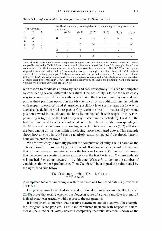
5 .5 the parameterized lens 117
Table 5.1. Profile and table example for computing the Dodgson score
(a) A profile.
1 2 3
d d cb a dc b aa c b
(b) The dynamic-programming table, T , for computing the Dodgson score ofcandidate a.
(0, 0) (0, 1) (0, 2) (1, 0) (1, 1) (1, 2)
0 0 ∞ ∞ ∞ ∞ ∞1 0 3 ∞ 1 3 ∞2 0 1 4 1 2 4
3 0 1 2 1 2 3
Note: The table at the right is used to compute the Dodgson score of candidate a in the profile at the left. In boththe profile here and in Table 5.2, our tabular vote displays are arranged “top down,” for example, the leftmostcolumn of this profile indicates that the vote of the first voter is d � b � c � a. The “1 2 3” on the top rowof profiles, both here and in Table 5.2, indicates the voters, for example, the column headed by a “3” is aboutvoter 3. In the profile given in part (a), the deficits of a with respect to the candidates b, c, and d are 0, 1, and2. So P = {c, d} and each column label refers to a’s deficits against c and d. The Dodgson score is the value,3, that is computed for the entry T (3, (1, 2)), and it is achieved by pushing a one position upward in the secondvote and two positions upward in the third vote.
with respect to candidates c and d by one and two, respectively. This can be computedby considering several different alternatives. One possibility is to use the least costlyway to decrease the deficit of a with respect to d in the first i − 1 votes by one and thenpush a three positions upward in the ith vote to cut by an additional one the deficitswith respect to each of c and d. Another possibility is to use the least costly way todecrease the deficit of a with respect to d by two in the first i − 1 votes and push a oneposition upward in the ith vote, to shrink by one its deficit with respect to c. A thirdpossibility is to just use the least costly way to decrease the deficits by 1 and 2 in thefirst i − 1 votes and leave the ith vote unaltered. The entry of the table corresponding tothe ith row and the column corresponding to the deficit decrease vector (1, 2) will storethe best among all the possibilities, including those mentioned above. This exampleshows how an entry in row i can be relatively easily computed if we already have inhand all the entries of row i − 1.
We are now ready to formally present the computation of entry T (i, d) based on theentries in row i − 1. We use L
ji (d) for the set of all vectors of decreases of deficits such
that if those decreases are satisfied over the first i − 1 votes of R then that will ensurethat the decreases specified in d are satisfied over the first i voters of R when candidatea is pushed j positions upward in the ith vote. We use hi to denote the number ofcandidates that voter i prefers to a. Then T (i, d) will be assigned the value stated bythe right-hand side below:
T (i, d) = min0�j�hi
mind ′∈L
ji (d)
{T (i − 1, d ′) + j}.
A completed table for an example with three votes and four candidates is provided asTable 5.1.
Using the approach sketched above and additional technical arguments, Betzler et al.(2010) prove that testing whether the Dodgson score of a given candidate is at most k
is fixed-parameter tractable with respect to the parameter k.It is important to mention that negative statements are also known. For example,
the Dodgson score problem is not fixed-parameter tractable with respect to param-eter n (the number of votes) unless a complexity-theoretic statement known as the
118 5 dodgson’s rule and young’s rule
exponential-time hypothesis is false. This follows from the fact that the problem isW[1]-hard (Fellows et al., 2010); W[1]-hardness is a central hardness notion in param-eterized complexity. Young elections are also intractable with respect to the scoreparameter, k. In particular, Betzler et al. (2010) prove that the StrongYoung scoreproblem is complete for the parameterized complexity class W[2].
5.6 Approximation Algorithms
We now focus specifically on Dodgson elections. Since Dodgson scores are hardto compute exactly in general, an alternative approach is to view the Dodgson scorecomputation as a combinatorial optimization problem and exploit the rich and beautifultheory of approximation algorithms (e.g., see Vazirani, 2001) in order to approximatethe Dodgson score. Briefly, the challenge is to obtain efficient (i.e., polynomial-time)algorithms that return scores that are provably close to the Dodgson score. Furthermore,such an approximation algorithm can be used as an alternative voting rule to Dodgson’srule under some circumstances. We discuss these issues below.
We consider algorithms that receive as input a candidate p from an m-candidate setA and an n-voter election profile R over A, and return a score for p. We denote thescore returned by an algorithm Y when applied on such an input by scY (p, R). Also,scD(p, R) will denote the Dodgson score. An algorithm Y is said to be a Dodgsonapproximation if scY (x, R) � scD(x, R) for every candidate x ∈ A and every profileR. Also, Y is said to have an approximation ratio of ρ � 1 if scY (x, R) � ρ · scD(x, R),for every candidate x and every profile R over A.
Let us give a trivial example. Again, denote by deficit(x, y, R) the deficit of candidatex with respect to candidate y in profile R, that is, the minimum number of voterswho have to change their preference so that x beats y in their pairwise election.Consider the algorithm Y that, given a candidate x and a preference profile R, returnsa score of scY (x, R) = (m − 1) ·∑y∈A−{x} deficit(x, y, R). It is easy to show that thisalgorithm is a Dodgson approximation and, furthermore, has approximation ratio atmost m − 1. In particular, it is possible to make x beat y in a pairwise election bypushing x to the top of the preferences of deficit(x, y, R) voters, and clearly thisrequires at most (m − 1) · deficit(x, y, R) sequential exchanges of adjacent candidates.By summing over all y ∈ A − {x}, we obtain an upper bound of scY (x, R) on theDodgson score of x. On the other hand, given x ∈ A, for every y ∈ A − {x} we requiredeficit(x, y, R) sequential adjacent-exchanges that push x above y in the preferencesof some voter in order for x to beat y in a pairwise election. Moreover, these sequentialadjacent-exchanges do not decrease the deficit with respect to any other candidate.Therefore,
∑y∈A−{x} deficit(x, y, R) � scD(x, R), and by multiplying by m − 1 we
get that scY (x, R) � (m − 1) · scD(x, R).
5.6.1 Achieving Logarithmic Approximation Ratios
In this section we present two Dodgson approximations with approximation ratioslogarithmic in the number of candidates. One is a combinatorial, greedy algorithm andthe other is an algorithm based on linear programming.
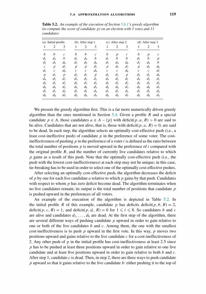
5 .6 approximation algorithms 119
Table 5.2. An example of the execution of Section 5.6.1’s greedy algorithm(to compute the score of candidate p) on an election with 3 votes and 11candidates
(a) Initial profile.
1 2 3
b b cd1 d4 bd2 d5 d6
c p d7
d3 c d8
p d1 pd4 d2 d1
d5 d3 d2
d6 d6 d3
d7 d7 d4
d8 d8 d5
(b) After step 1.
1 2 3
b b cd1 d4 bd2 d5 d6
p p d7
c c d8
d3 d1 pd4 d2 d1
d5 d3 d2
d6 d6 d3
d7 d7 d4
d8 d8 d5
(c) After step 2.
1 2 3
b p cd1 b bd2 d4 d6
p d5 d7
c c d8
d3 d1 pd4 d2 d1
d5 d3 d2
d6 d6 d3
d7 d7 d4
d8 d8 d5
(d) After step 3.
1 2 3
b p cd1 b pd2 d4 bp d5 d6
c c d7
d3 d1 d8
d4 d2 d1
d5 d3 d2
d6 d6 d3
d7 d7 d4
d8 d8 d5
We present the greedy algorithm first. This is a far more numerically driven greedyalgorithm than the ones mentioned in Section 5.4. Given a profile R and a specialcandidate p ∈ A, those candidates a ∈ A − {p} with deficit(p, a, R) > 0 are said tobe alive. Candidates that are not alive, that is, those with deficit(p, a, R) = 0, are saidto be dead. In each step, the algorithm selects an optimally cost-effective push (i.e., aleast cost-ineffective push) of candidate p in the preference of some voter. The cost-ineffectiveness of pushing p in the preference of a voter i is defined as the ratio betweenthe total number of positions p is moved upward in the preference of i compared withthe original profile R, and the number of currently live candidates relative to whichp gains as a result of this push. Note that the optimally cost-effective push (i.e., thepush with the lowest cost-ineffectiveness) at each step may not be unique; in this case,tie-breaking has to be used in order to select one of the optimally cost-effective pushes.
After selecting an optimally cost-effective push, the algorithm decreases the deficitof p by one for each live candidate a relative to which p gains by that push. Candidateswith respect to whom p has zero deficit become dead. The algorithm terminates whenno live candidates remain; its output is the total number of positions that candidate p
is pushed upward in the preferences of all voters.An example of the execution of the algorithm is depicted in Table 5.2. In
the initial profile R of this example, candidate p has deficits deficit(p, b, R) = 2,deficit(p, c, R) = 1, and deficit(p, di, R) = 0 for 1 � i � 8. So candidates b and c
are alive and candidates d1, . . . , d8 are dead. At the first step of the algorithm, thereare several different ways of pushing candidate p upward in order to gain relative toone or both of the live candidates b and c. Among them, the one with the smallestcost-ineffectiveness is to push p upward in the first vote. In this way, p moves twopositions upward and gains relative to the live candidate c for a cost-ineffectiveness of2. Any other push of p in the initial profile has cost-ineffectiveness at least 2.5 sincep has to be pushed at least three positions upward in order to gain relative to one livecandidate and at least five positions upward in order to gain relative to both b and c.After step 1, candidate c is dead. Then, in step 2, there are three ways to push candidatep upward so that it gains relative to the live candidate b: either pushing it to the top of

120 5 dodgson’s rule and young’s rule
the first vote (this has cost-ineffectiveness 5 because p would have moved five posi-tions in total compared to the initial first vote), or pushing it to the top of the secondvote (with cost-ineffectiveness 3), or pushing it four positions upward in the third vote(with cost-ineffectiveness 4). The algorithm picks the second option. Then, in step 3,the algorithm can either push candidate p to the top of the first vote or push it fourpositions upward in the third vote. The former has a cost-ineffectiveness of 5 (recallthat cost-ineffectiveness is defined using the total number of positions p would movecompared to its position at the initial profile), while the latter has a cost-ineffectivenessof 4 and is the push the algorithm picks. After step 3, all candidates are dead and thealgorithm terminates by returning the total number of positions p is pushed upward,that is, 9.
Since the algorithm terminates when all candidates in A − {p} are dead, it is clearthat p becomes a Condorcet winner. The analysis of this greedy algorithm uses a linearprogramming relaxation of the Dodgson score. Given the profile R with a set of votersN and a set of m candidates A, denote by ri the rank of candidate p in the preference ofvoter i. For every voter i ∈ N , denote by S i the subcollection that consists of the sets Si
k
for k = 1, . . . , ri − 1, where the set Sik contains the live candidates that appear in posi-
tions ri − k to ri − 1 in the preference of voter i. We denote by S the (multiset) unionof the subcollections S i for i ∈ N . The problem of computing the Dodgson score ofcandidate p on profile R is equivalent to selecting sets from S of minimum total size sothat at most one set is selected among the ones in S i for each voter i and each candidatea ∈ A − {p} appears in at least deficit(p, a, R) selected sets. This can be expressed byan integer linear program using a binary variable x(S) to denote whether the set S ∈ Shas been selected. We present the relaxation of this LP below, where the integralityconstraint for the variables has been relaxed to fractional values between 0 and 1:
Minimize∑i∈N
ri−1∑k=1
k · x(Sik)
subject to ∀a ∈ A − {p},∑i∈N
∑S∈S i :a∈S
x(S) � deficit(p, a, R)
∀i ∈ N,∑S∈S i
x(S) � 1
∀S ∈ S, 0 � x(S) � 1.
Clearly, the Dodgson score of candidate p is an upper bound on the optimal objectivevalue of this LP.
The analysis uses a technique that is known as dual fitting and is similar to theanalysis of a greedy algorithm for the related constrained set multicover problem; seeRajagopalan and Vazirani (1999) and Vazirani (2001, pp. 112–116). The idea is touse the decisions taken by the algorithm and construct a feasible solution for the dual(maximization) LP that has value at most the score returned by the algorithm dividedby Hm−1, where Hk = 1 + 1
2 + · · · + 1k
denotes the kth harmonic number. By a simpleduality argument, this implies that the score returned by the algorithm is at most Hm−1
times the optimal objective value of the above LP and, consequently, at most Hm−1
times the Dodgson score of p.
5 .6 approximation algorithms 121
This suggests a different algorithm, in particular, an LP-based algorithm for approx-imating the Dodgson score of a candidate p without explicitly providing a way ofpushing p upward in the preferences of some voters in a way making p become theCondorcet winner. This algorithm just uses the LP relaxation above, computes its opti-mal objective value, and returns this value multiplied by Hm−1 as a score for candidatep. Then the approximation ratio of Hm−1 is obvious. The algorithm is also a Dodgsonapproximation, since the score returned by this section’s greedy algorithm (which isan upper bound for the Dodgson score of p) is not higher than the score returned bythe LP-based algorithm. The following statement summarizes our discussion.
Theorem 5.6 (Caragiannis et al., 2012b). This section’s greedy algorithm and LP-based algorithm are Dodgson approximations, each with approximation ratio Hm−1.
5.6.2 Approximation Algorithms as Alternative Voting Rules?
A Dodgson approximation naturally induces a voting rule by electing the candidate(s)with minimum score. Arguably, such a voting rule maintains some echo of the basicphilosophy behind Dodgson’s election system—more strongly so if it is a very goodapproximation. But can it really be used as a voting rule? Trying to support a yes answerto this question requires us to discuss an issue that we have not yet touched on. Onecan argue that for a voting rule to be attractive, it should not only be easy to compute,but also, ideally, should have certain properties that are considered desirable from asocial-choice point of view. Several such properties are not satisfied by Dodgson’srule, and this is the main reason why the rule has been criticized in the social-choiceliterature, see, for example, Brandt (2009a) and the references therein.
We will see that Dodgson approximations, in return for their core disadvantage ofmerely being an approximation to Dodgson’s rule, can satisfy desirable social-choiceproperties, even while also providing polynomial-time algorithms. Before going onto the three social-choice properties we will discuss, it is important to make clearjust how greatly Dodgson approximations can distort Dodgson’s rule, especially sincewe commented above that Dodgson approximations in some way echo the flavor andphilosophy of Dodgson. The best Dodgson approximation we consider in this sectionhas an approximation ratio of 2. Consider a three-candidate election for which theactual Dodgson scores of the candidates are 10, 11, and 12. A Dodgson approximationhaving ratio 2 could give for these candidates, respectively, scores of 18, 16, and 14.That is, the ordering of even an excellent Dodgson approximation can be a completeinversion of the actual Dodgson ordering, and the worst Dodgson loser can be namedthe unique winner. Clearly, the fact that even a 1.000001 approximation-ratio algorithmcan completely invert the entire ranking of the candidates is a troubling (but not farfrom unavoidable—see the discussion at the end of Section 5.6.3) feature of usingapproximations as voting rules.
In the following, when we say that a Dodgson approximation satisfies a social-choiceproperty we are referring to the voting rule induced by the algorithm. As a warm up,observe that the voting rule induced by any Dodgson approximation (regardless of itsapproximation ratio) is Condorcet-consistent, basically because anything times zerois zero. So every Dodgson approximation, regardless of how bad its ratio is, must

122 5 dodgson’s rule and young’s rule
assign score of 0 to any Condorcet winner. But since Dodgson approximations neverunderestimate scores, any candidate who is not a Condorcet winner will be assigned ascore of at least 1. So any Condorcet winner will be the one and only winner under anyDodgson approximation. (Thank goodness Dodgson did not add a one in the definitionof his scores. That would destroy the above claim, which is deeply dependent on thespecial nature of zero.) Of course, Dodgson’s system itself also is Condorcet-consistent.
We will now move on to discuss two other socially desirable properties: monotonicityand homogeneity. We will see that these properties can be achieved by good Dodgsonapproximations that run in polynomial time.
A voting rule is said to be monotonic if a winning candidate always remains winningafter it is pushed upward in the preferences of some of the voters. Dodgson’s rule isknown to be monotonic when there are at most three candidates and to be nonmonotonicfor each number of candidates greater than or equal to four (Fishburn, 1982, p. 132).The intuition for the latter is that if a voter ranks x directly above y and y above z,exchanging x and y may not help y if it already beats x, but may help z defeat x. Thetwo approximation algorithms presented in Section 5.6.1 are also nonmonotonic.
In contrast, the Dodgson approximation that returns (m − 1) ·∑y∈A−{x}deficit(x, y, R) as the score of candidate x is monotonic as a voting rule. Indeed,consider a preference profile R and a winning candidate x. Pushing x upward inthe preferences of some of the voters can neither increase its score (since its deficitwith respect to each other candidate does not increase) nor decrease the score of anyother candidate y ∈ A − {x} (since the deficit of y with respect to each candidate inA − {x, y} remains unchanged and its deficit with respect to x does not decrease). Sowe already have a monotonic Dodgson approximation with approximation ratio m − 1.In the following we present much stronger results.
A natural “monotonization” of Dodgson’s voting rule yields a monotonic Dodg-son approximation with approximation ratio of 2. The main idea is to define thewinning set of candidates for a given profile first and then assign the same score tothe candidates in the winning set and a higher score to the nonwinning candidates.Roughly speaking, the winning set is defined so that it contains the Dodgson win-ners for the given profile as well as the Dodgson winners of other profiles that arenecessary so that monotonicity is satisfied. More formally put, we say that an n-voteelection profile R′ is a y-improvement of profile R for some candidate y ∈ A if R′ isobtained by starting from R and pushing y upward in the preferences of zero or morevoters.
Monotonization proceeds as follows. Let M denote the new voting rule we areconstructing. Denote by W (R) the set of winners of M (or the winning set) for profile R;we will soon specify which candidates belong to W (R). Let � = maxy∈W (R) scD(y, R).The voting rule M assigns a score of scM (y, R) = � to each candidate y ∈ W (R) anda score of
scM (y, R) = max{� + 1, scD(y, R)}to each candidate y /∈ W (R). All that remains is to define the winning set W (R). Thisis done as follows: For each profile R∗ and each Dodgson winner y∗ of R∗, include y∗
in the winning set W (R′) of each profile R′ that is a y∗-improvement of R∗.
5 .6 approximation algorithms 123
Theorem 5.7 (Caragiannis et al., 2014b). M is a monotonic Dodgson approximationwith an approximation ratio of 2.
That M is monotonic and is a Dodgson approximation follow immediately fromthe definitions of the winning set W (R) and the scores returned by M . The proof ofthe approximation ratio bound is based on the following technical property: Pushing acandidate y upward does not increase his or her Dodgson score and does not decreasethe Dodgson score of any other candidate by a factor larger than 2. The upper boundprovided by Theorem 5.7 is the best possible: No monotonic Dodgson approximationcan have an approximation ratio smaller than 2. This negative statement does not use anycomplexity-theoretic assumptions and actually holds for exponential-time algorithmsas well. Actually, monotonization (in the rather naive approach described above) yieldsan exponential-time algorithm.
So from the computational point of view, the above algorithm is not at all satisfactory.Fortunately, a polynomial-time implementation of monotonization is possible, althoughit involves an unavoidable (see Section 5.6.3) logarithmic loss in the approximationratio. There are two main obstacles that one has to overcome in order to implementmonotonization in polynomial time. First, as discussed in Section 5.3, computingthe Dodgson score and deciding whether a given candidate is a Dodgson winnerare computationally hard problems. This obstacle can be overcome using the scorereturned by the polynomial-time LP-based Dodgson approximation that we presentedin Section 5.6.1 instead of using the Dodgson score itself. Even in this case, givena profile R, we still need to be able to detect when a candidate y is the winneraccording to the LP-based voting rule in some profile R′ of which the current one isa y-improvement; if this is the case, y has to be included in the winning set W (R)of profile R. This means that exponentially many profiles may have to be checked inorder to determine the winning set of the current profile. This obstacle is overcomeby Caragiannis et al. (2014b) using the notion of pessimistic estimators. These arequantities defined in terms of the current profile only and are used to identify thewinning set in polynomial time. The next statement follows using these two high-levelideas and additional technical arguments.
Theorem 5.8 (Caragiannis et al., 2014b). There exists a monotonic polynomial-timeDodgson approximation with an approximation ratio of 2Hm−1.
Let us now turn to homogeneity. A voting rule is said to be homogeneous if, forevery integer k � 2, its outcome does not change when replacing each vote in thepreference profile with k identical copies of the vote. Fishburn (1977) observed thatDodgson’s rule is not homogeneous. The intuition behind this is that if candidates x
and y are tied in a pairwise election the deficit of x with respect to y does not increaseby duplicating the profile, but if x strictly loses to y in a pairwise election then thedeficit scales with the number of copies.
Tideman (2006, pp. 199–201) presents the following simplified version of Dodgson’srule and proves that it is both homogeneous and monotonic. A Condorcet winner—ifone exists—in an election profile R is the sole winner according to Tideman’s rule.

124 5 dodgson’s rule and young’s rule
Otherwise, the rule assigns a score of
scTd(x, R) =∑
y∈A−{x}max {0, n − (2 · ‖{i ∈ N : x �i y}‖)}
to each candidate x, and the candidate(s) with the minimum score win. In the aboveequation, the notation x �i y indicates that voter i prefers candidate x to candidate y.Unfortunately, this score definition does not provide a Dodgson approximation. Forexample, a candidate who is tied with some candidates and beats the rest has a scoreof 0, yet 0 is lower than its Dodgson score. However, we in fact can give a differentscoring framework, Td′, that is a Dodgson approximation and that will elect exactlythe same winners as does Tideman’s simplified variant of Dodgson’s rule (and thuswill be monotonic and homogeneous). Td′ is defined as follows. If a candidate x is aCondorcet winner, then it has score scTd′(x, R) = 0. Otherwise, Td′ “scales” the scoreof x as follows:
scTd′(x, R) = m · scTd(x, R) + m(1 + log m).
Clearly, scTd′(x, R) can be computed in time polynomial in n and m.
Theorem 5.9 (Caragiannis et al., 2014b). Td ′ is a monotonic, homogeneous,polynomial-time Dodgson approximation with an approximation ratio of O(m log m).
This approximation ratio is the best possible; a matching �(m log m) lower boundholds for any algorithm that is homogeneous (Caragiannis et al., 2014b).
5.6.3 Hardness of Approximation
The best polynomial-time Dodgson approximations presented in Section 5.6.1achieve—keeping in mind that Hm = ln n + �(1)—asymptotic approximation ratiosof O(log m). Under standard assumptions about NP, all polynomial-time Dodgsonapproximations have approximation ratios that are �(log m), so the above-mentionedapproximations from the previous section have ratios that are optimal within a constant,and in fact that constant can be kept down to 2. This claim is implicit in McCabe-Dansted(2006). Later, Caragiannis et al. (2012b) explicitly obtained and stated the followingresult, using a reduction from minimum set cover and well-known inapproximabilitythresholds of Feige (1998) and Raz and Safra (1997).
Theorem 5.10 (Caragiannis et al., 2012b). There exists a constant β > 0 such thatit is NP-hard to approximate the Dodgson score of a given candidate in an electionwith m candidates to within a factor of β ln m. Furthermore, for any ε > 0, thereis no polynomial-time
(12 − ε
)ln m-approximation for the Dodgson score of a given
candidate unless all problems in NP have algorithms running in time kO(log log k), wherek is the input size.
One might wonder why our particular notion of approximation has been used.For example, a natural alternative approach would be to approximate some notionof Dodgson ranking. Unfortunately, the following statement shows that this is animpossible goal: Efficient approximation algorithms for Dodgson ranking are unlikelyto exist. For the purpose of the theorem below, a Dodgson ranking of an election
5 .7 bibliography and further reading 125
instance is an ordering of the candidates such that if i < j then the ith candidate in theordering has Dodgson score no greater than the j th candidate in the ordering.
Theorem 5.11 (Caragiannis et al., 2012b). Given a profile with m candidates and aspecial candidate p, it is NP-hard to decide whether p is a Dodgson winner or hasrank at least m − 6
√m in any Dodgson ranking.
5.7 Bibliography and Further Reading
Dodgson’s election system first appeared in Dodgson’s 1876 pamphlet (Dodgson,1876). The computational complexity of the winner problem for Dodgson’s systemwas shown NP-hard in the seminal paper of Bartholdi et al. (1989b), and was shown�
p2 -complete by Hemaspaandra et al. (1997a), see also Brandt et al. (2010b, p. 54).
Young’s election system was defined by him in 1977 (Young, 1977), and the complexityof StrongYoung was pinpointed as being �
p2 -complete by Rothe et al. (2003). See
Brandt (2009a) and the references therein for perspectives on why Dodgson proposedhis system and discussions of Dodgson’s system in terms of not satisfying certainproperties.
A number of other papers discuss the complexity of Dodgson and Young electionsor variants of those elections (Hemaspaandra et al., 2009; Brandt et al., 2010a, 2010b,2015b). Readers interested in the complexity of these election systems may be interestedin the work showing that Kemeny’s election system (Kemeny, 1959; Kemeny and Snell,1960)—see also Chapter 4—has a �
p2 -complete winner problem (Hemaspaandra
et al., 2005) and a �p2 -complete unique winner problem (Hemaspaandra et al., 2009).
Complexity has also been broadly used as a tool with which to block attacks onelections, such as manipulation (Bartholdi et al., 1989a), bribery (Faliszewski et al.,2009b), and control (Bartholdi et al., 1992); see Chapters 6 and 7, and see also thesurveys by Faliszewski et al. (2009d, 2010).
�p2 , in its “logarithmic number of sequential queries to NP” definition, was first
studied in the early 1980s, by Papadimitriou and Zachos (1983). Hemachandra (1989)showed that that definition yields the same class of sets as the unbounded-paralleldefinition. �
p2 -completeness can also apply to a range of problems quite different
from the election problems discussed in this chapter. For example, determining whengreedy algorithms well-approximate maximum independent sets is known to be �
p2 -
complete (Hemaspaandra and Rothe, 1998). The most important tool for proving �p2 -
completeness is Lemma 5.3, due to Wagner (1987). Readers more generally interestedin complexity will find an excellent, accessible introduction in the textbook of Bovetand Crescenzi (1993), and a more advanced and technique-based tour is provided byHemaspaandra and Ogihara (2002).
The material presented in our heuristics section (Section 5.4) is based on the workof Homan and Hemaspaandra (2009) about using greedy heuristics for Dodgson elec-tions. The independent work of McCabe-Dansted et al. (2008) studies the use ofgreedy heuristics for WeakDodgson elections. The two papers are based on the samecentral insight and obtain related results. However, there are some nontrivial differ-ences between the two papers and their claims; these differences are discussed in detailin Section 1 of Homan and Hemaspaandra (2009).
126 5 dodgson’s rule and young’s rule
Readers interested in the theory of parameterized computational complexity canfind a systematic treatment in textbooks such as the ones by Downey and Fellows(1999) and Niedermeier (2006). Betzler et al. (2012) survey the progress in that field inrelation to voting and cover both winner determination and other problems, for severalvoting rules.
The first approximation algorithms for voting rules (e.g., Kemeny) are implicit inthe papers of Ailon et al. (2005), Coppersmith et al. (2006), and Kenyon-Mathieu andSchudy (2007). The material presented in Section 5.6 is from Caragiannis et al. (2012b,2014b). Several interesting results have not been covered. For example, as an alterna-tive to Tideman’s simplified Dodgson rule, the maximin voting rule yields a Dodgsonapproximation with approximation ratio m2 (Faliszewski et al., 2011b). Caragianniset al. (2014b) discuss additional social-choice properties that are more difficult thanmonotonicity to achieve by good Dodgson approximations. Finally, observe that Sec-tion 5.6 does not contain any results related to Young’s rule. Unfortunately, such good(polynomial-time) approximations are unlikely to exist. For example, unless P = NP,the StrongYoung score is not approximable within any factor by polynomial-timealgorithms (Caragiannis et al., 2012b).
Acknowledgments
We are grateful to Markus Brill, Jorg Rothe, and the editors for helpful suggestionson an earlier version. Any remaining errors are the sole responsibility of the authors.We appreciatively acknowledge the support of grants NSF-CCF-0915792, NSF-CCF-1101452, and NSF-CCF-1101479.
CHAPTER 6
Barriers to Manipulationin Voting
Vincent Conitzer and Toby Walsh
6.1 Introduction
In many situations, voters may vote strategically. That is, they may declare preferencesthat are not their true ones, with the aim of obtaining a better outcome for themselves.The following example illustrates this.
Example 6.1. Consider an election with three alternatives, a, b, and c, and three voters,1, 2, and 3. Suppose the rule used is plurality—an alternative gets a point each timeit is ranked first by a voter, and the alternative with the most points wins—with tiesbroken toward alternatives earlier in the alphabet. Suppose voter 3 knows (or stronglysuspects) that voter 1 will rank a first in her vote, and that voter 2 will rank b first.Voter 3’s true preferences are c � b � a. If she votes truthfully, this will result in athree-way tie, broken in favor of a which is 3’s least preferred alternative. If, instead,voter 3 ranks b first, then b will win instead. Hence, voter 3 has an incentive to cast avote that does not reflect her true preferences.
This is often referred to as manipulation or strategic voting; we will use “manip-ulation” throughout.1 Voting rules that are never manipulable are also referred to asstrategyproof. We start by reviewing the Gibbard-Satterthwaite impossibility result(discussed also in Chapter 2), which states that with unrestricted preferences over threeor more alternatives, only very unnatural rules are strategyproof. The main focus of thechapter is on exploring whether computational complexity can be an effective barrierto manipulation. That is, we may not be concerned about manipulation of a voting ruleif it is computationally hard to discover how to manipulate it.
1 Of course, one may disagree, at least in some circumstances, that strategic voting is really “manipulative” inthe common sense of the word. We simply use “manipulation” as a technical term equivalent to strategicallyreporting one’s preferences incorrectly. Nevertheless, we will give some reasons why it can be undesirable inwhat follows.
127
128 6 barriers to manipulation in voting
6.2 Gibbard-Satterthwaite and Its Implications
An important axiomatic result about the properties of voting rules is the Gibbard-Satterthwaite Theorem:
Theorem 6.2 (Gibbard, 1973; Satterthwaite, 1975). Consider a (resolute)2 votingrule that is defined for some number m of alternatives with m � 3, with no restrictionson the preference domain. Then, this rule must be at least one of the following:
1. dictatorial: there exists a single fixed voter whose most-preferred alternative is chosenfor every profile;
2. imposing: there is at least one alternative that does not win under any profile;3. manipulable (i.e., not strategyproof).
Properties 1 and 2 are not acceptable in most voting settings. Hence, under theconditions of the theorem, we are stuck with property 3: there will exist profiles suchthat at least one of the voters has an incentive to misreport her preferences.
Before discussing how we might address this, we should first discuss why manipu-lability is a significant problem. It may not seem so. For example, consider a pluralityelection with three alternatives. If one of the candidates3 is considered to have a poorchance of winning the election (consider, for example, a third party in the UnitedStates), then everyone might vote for one of the other two candidates, in order to avoidwasting their votes. Is this a significant problem? Will it not simply result in the samewinner that plurality-with-runoff (or STV)4 would have chosen (if everyone had votedtruthfully), and is that so bad? Additionally, there are those who argue that democratsshould not be worried about manipulation (Dowding and Hees, 2008). There are,however, several potential downsides to such manipulation, including the following.(Formalizing all these downsides would go beyond the scope of this chapter, so wepresent them informally; we hope the reader would be able to formalize these conceptsif needed.)
� Bad equilibria. In the above example, it is not at all clear that the resulting winner willbe the same as the true plurality-with-runoff winner. All that is required is that votersexpect the third alternative to have poor chances. It is possible that this alternative isactually very much liked across the electorate, but nobody is aware of this. Even morestrikingly, it is possible that everyone is aware of this, and yet the alternative is expectedto perform poorly—for example, because nobody is aware that others are aware of thealternative’s popularity. Hence, an alternative that is very much liked, and perhaps wouldhave won under just about any reasonable rule had everyone voted truthfully, may notwin.
2 Recall that a voting rule is resolute if it returns only a single alternative for every profile.3 We use “alternatives” and “candidates” interchangeably.4 Recall that under the plurality-with-runoff rule, the alternatives with the top two plurality scores proceed to
a runoff round, and the one that is preferred to the other by more voters wins. Under STV (also known asInstant Runoff Voting), only the alternative with the lowest plurality score is eliminated in each round; it is thenremoved from all the votes, so that votes that ranked it first now rank another alternative first. This procedureis repeated until only one alternative—the winner—remains. (For an axiomatization of this rule, see Freemanet al. (2014).)
6 .3 noncomputational avenues 129
� Lack of information. Even if the bad equilibria described above are in fact avoided, wecannot be sure that this is the case, because we will never know exactly how popularthat third alternative really was. This also interferes with the process of identifying moredesirable alternatives in the next election.
� Disenfranchisement of unsophisticated voters. Voters who are less well informed mayend up casting less effective votes than those who are well informed (for example,votes for the third alternative). Knowledge is power—but in many elections, this is notconsidered desirable.
� Wasted effort. Even if all agents manipulate to the same extent, still much effort, whetherof the computational, information gathering, or communicational variety, is expendedin figuring out how to manipulate well, and presumably this effort could have been moreproductively spent elsewhere. This can be seen as a type of tragedy of the commons;everyone would be better off if nobody spent effort on manipulation, but individuallyvoters are still better off manipulating.
In the theory of mechanism design—which applies not only to the design of votingrules but also to that of auctions, matching mechanisms, and any other setting wherea decision must be made based on the preferences of multiple strategic agents—thereis generally a focus on designing mechanisms in which agents have no incentiveto misreport their preferences. This is justified by a result known as the revelationprinciple. Stating it formally here would take us too far afield, but roughly speaking,it says that for any mechanism that results in a good equilibrium (in a game-theoreticsense), there exists another mechanism that results in the same outcomes, but in whichagents report their preferences directly and they have no incentive to misreport them.5
That is, at some level, we should be able to get incentives to report truthfully (i.e.,use a truthful mechanism) for free. The revelation principle has been criticized on thebasis that it implicitly assumes agents to be computationally unbounded, and indeed ithas been shown that in some cases there exist mechanisms (that are not truthful) thatwill perform at least as well as any truthful mechanism, and strictly better if agents areunable to compute their strategically optimal actions (Conitzer and Sandholm, 2004).
Taken together, there seem to be several arguments for attempting to erect barriers tomanipulation. However, the Gibbard-Satterthwaite Theorem poses a fundamental limitto such barriers. How can we get around it? We will first discuss some avenues thatare not computational in nature. Then, we devote most of the chapter to computationalavenues.
6.3 Noncomputational Avenues around Gibbard-Satterthwaite
One way of sidestepping the Gibbard-Satterthwaite Theorem is to restrict the domainof preferences. Probably the best-known such restriction is that of single-peaked
5 It should be noted that the notion of not having any incentive to misreport here is weaker than strategyproofness.Rather, it is Bayes-Nash equilibrium, which means that an agent is best off telling the truth in expectation overa prior distribution over the other agents’ preferences—but the agent might be better off misreporting for aparticular realization of the reports. There is a version of the revelation principle that results in a strategyproofmechanism, but this requires the original mechanism to have dominant strategies for all agents.
130 6 barriers to manipulation in voting
preferences. Here, the assumption is that there exists an ordering < of the alternatives—for example, political candidates may be ordered on the left-to-right political spectrum,or the alternatives may be tax rates, locations along a single road, and so on. More-over, the following assumption is made: if voter i’s most-preferred alternative is a,and a < b < c or c < b < a, then b �i c (i prefers b to c). In this case (assuming,for simplicity, an odd number of voters) consider the median voter rule: order the vot-ers by their most-preferred alternatives, and choose the median voter’s most-preferredalternative. (Note that this rule does not require voters to specify preferences beyondtheir top choice.) This rule is strategyproof and always elects a Condorcet winner6. Ofcourse, the usefulness of this result is limited by the fact that we cannot simply makethe voters’ preferences single-peaked when they are not. We could declare any vote thatis not single-peaked invalid, but this just comes down to forcing voters to manipulate.For more discussion of single-peaked preferences, see Chapter 2.
Another possible avenue is to use randomized rules, which map every profile ofvotes to a probability distribution over the alternatives. For example, if we break theties of a voting rule randomly, then we have a randomized voting rule. However, thereare many other ways to obtain a randomized voting rule. The Gibbard-SatterthwaiteTheorem above applies to deterministic rules only, so one might hope that randomizedrules are not subject to such an impossibility. Unfortunately, as it turns out, there isa subsequent result by Gibbard that generalizes the Gibbard-Satterthwaite Theoremto randomized rules. To present this result, we first need to define strategyproofnessin the context of randomized rules, and for that, we need to define preferences overlotteries over alternatives. For example, if a voter’s preferences are a � b � c, shouldthe voter prefer b, or a 50-50 lottery over a and c? Both could be reasonable. Forexample, if the voter has utilities 3, 2, and 0 for the alternatives respectively, b wouldgive higher expected utility (2 > 1.5), but if the voter has utilities 3, 1, and 0, then the50-50 lottery over a and c gives higher utility (1.5 > 1). Therefore, in this context,a quite conservative definition of strategyproofness is often used: a randomized ruleis strategyproof if and only if for every utility function over the alternatives that isconsistent with the voter’s preferences over the (pure) alternatives, the voter maximizesher utility by reporting these true preferences (regardless of how the others vote).7 Wecan now present Gibbard’s result:
Theorem 6.3 (Gibbard, 1977). If there are no restrictions on the preference domain,any strategyproof randomized rule is a randomization over a collection of the followingtypes of rules:
� unilateral rules, under which at most one voter’s vote affects the outcome;� duple rules, under which there are at most two alternatives that have a possibility of
winning (i.e., that win under some profile).
The result makes it clear that randomization is not the answer to all our problems. Acoin flip results in the discarding of all but one of the votes, or in the discarding of all
6 Recall that an alternative a is a Condorcet winner if it wins all its pairwise contests. That is, for every otheralternative b, more voters prefer a to b than vice versa.
7 For studies of other ways of extending strategyproofness to randomized voting rules, see Aziz et al. (2013d)and Aziz et al. (2014c).

6 .4 computational hardness as a barrier to manipulation 131
but two of the alternatives. In many situations, these rules will not be acceptable. Still,the result allows for some randomized rules that are perhaps not entirely unreasonable.For example, we can randomly choose a dictator (the theorem implies that, withthree or more alternatives, this is in fact the only way to guarantee a Pareto-optimaloutcome), or randomly choose two alternatives and have a majority election betweenthem. Barbera (1979) gives some characterizations of randomized strategyproof rulesas well; these are consistent with Gibbard’s result above, but seem to cast the rulesin a more positive light. More recently, Procaccia (2010) studied the extent to whichstrategyproof randomized rules can achieve formal approximations to the scores fromcommon voting rules.
A final possible avenue is to use irresolute rules, which return a set of alternatives(possibly larger than one) and leave it at that. Can such a rule be strategyproof (andsimultaneously reasonable)? To make sense of this question, we first need to saysomething about what an agent’s preferences over sets of alternatives can be. Buildingon earlier results, Brandt (2011b) and Brandt and Brill (2011) have recently providedresults that show that various irresolute rules are in fact strategyproof with respect tovarious extensions of preferences to sets of alternatives.8 While these positive resultsare encouraging, they do face a major limitation. In many voting settings, in the end, werequire a single winning alternative. If we add any procedure for going from the winningset of alternatives to a single one—for example, choosing the lexicographically firstalternative in the set—then the combination of the irresolute rule and the subsequentprocedure is a resolute rule, and we run right back into the Gibbard-Satterthwaiteimpossibility result. Similarly, if we randomly choose from the winning set, we runinto the impossibility results for randomized rules. Thus, for these positive results toapply, the procedure for going from the selected set of alternatives to a single alternativefundamentally needs to remain unspecified, and moreover the voters need to respondto this lack of information in a particular way. For more detail, see Chapter 3.
6.4 Computational Hardness as a Barrier to Manipulation
Another potential barrier to manipulation is computational hardness. Even if we cannotprevent a voting rule from being manipulable in principle, this may not be a significantconcern as long as determining how to manipulate it is computationally prohibitive.
The argument that the complexity of computing a manipulation might be a barrier tostrategic voting was first put forward in an influential paper by Bartholdi et al. (1989a).A whole subfield of social choice has since grown from this proposal, studying thecomputational complexity of manipulating different voting rules under several differentassumptions (e.g., Conitzer et al., 2007). For two recent surveys, see Faliszewski et al.(2010) and Faliszewski and Procaccia (2010); Brandt et al. (2013a) also discuss thetopic at some length. In the remainder of this section, we discuss this line of work inmore detail.
8 Other extensions lead to negative results (Duggan and Schwartz, 2000). For more on strategyproofness andother notions of monotonicity in this context, see Sanver and Zwicker (2012) and the references cited in thatwork.

132 6 barriers to manipulation in voting
6.4.1 The Basic Variant
The original paper (Bartholdi et al., 1989a) defined a basic model which has since beeninvestigated extensively. We suppose all but one voter, the manipulator, have voted andthat these votes and the rule to be used are known to the manipulator. We ask whetherit is possible for the manipulator to ensure that a given alternative wins. More formally,we can define the following decision problem.
Manipulation Problem
Given. A profile of votes � cast by everyone but the manipulator, and a preferred alternative a.Question. Is there a vote that the manipulator can cast so that a wins?
This problem is typically in NP as a simple witness is a vote that ensures a wins.Supposing that the voting rule is polynomial to execute,9 this witness can be checkedin polynomial time. There is also a destructive variant of this question, where weask if it is possible for the manipulator to cast a vote so that a given alternative doesnot win. Note that these problems correspond exactly to the predicament of voter 3in Example 6.1, with the exception that the question is now whether she can makea particular alternative win. One may wonder if a more natural problem would beto determine the best (according to her own true preferences) alternative that she canmake win. This problem is effectively equivalent; to answer it, it is sufficient to evaluatefor each of the alternatives in turn whether she can make it win (and, conversely, itis necessary to at least evaluate whether she can make her most-preferred alternativewin).
Of course, when the rule is plurality, this problem is computationally trivial: to see ifyou can make alternative a win, it suffices to see what would happen if you submitteda vote that ranks a first. Indeed, for many rules, the problem is in P. Bartholdi et al.(1989a) provided an algorithm that solves the problem in polynomial time for manyvoting rules.
Definition 6.1. Say that a voting rule satisfies the BTT conditions if
1. it can be run in polynomial time,2. for every profile � and every alternative a, the rule assigns a score S(�, a) to a,3. for every profile �, the alternative with the maximum score wins,10 and4. the following monotonicity condition holds: for any �,�′, for any alternative a, if for
each voter i we have that {b : a �i b} ⊆ {b : a �′i b}, then S(�, a) � S(�′, a). (That
is, if we modify a vote in a way that does not rank anyone ahead of a that was previouslyranked behind a, then a’s score cannot have decreased.)
Theorem 6.4 (Bartholdi et al., 1989a). The manipulation problem can be solved inpolynomial time for any rule satisfying the BTT conditions.
The algorithm for constructing a manipulator vote that successfully makes alterna-tive a win (if any such vote exists) is quite straightforward. Rank a first. For the next
9 See earlier chapters in the book for discussion of rules for which this is not the case.10 Assume, say, a fixed tie-breaking order.
6 .4 computational hardness as a barrier to manipulation 133
position in the vote, find some remaining alternative b that can be ranked there so thata still wins. (To check this, complete the rest of the vote arbitrarily, and calculate b’sscore; by the monotonicity condition above, a and b’s scores will not depend on howthe rest of the vote is completed. This is because if we change the relative orderingof the remaining alternatives, this is a modification that satisfies the condition, and socannot decrease a or b’s score; it can also not increase these scores, because then thereverse modification would decrease it.) If no such alternative can be found, declarefailure; if the vote is completed, declare success; otherwise, repeat for the next position.This algorithm applies not only to positional scoring rules such as plurality and Borda,but also to rules such as Copeland and maximin.11
Bartholdi et al. (1989a) were also the first to show that the problem is NP-hard forsome rules. Specifically, they showed NP-hardness for manipulating the second-orderCopeland rule, under which an alternative’s score is the sum of the Copeland scores ofthe alternatives that it defeats. (Note that this way of scoring violates the third conditionabove: if in some vote, we change the relative ordering of the alternatives ranked (say)behind a only, this can affect those alternatives’ Copeland scores, and thereby a’ssecond-order Copeland score.) They also showed NP-hardness of manipulation for the(first-order) Copeland rule when ties are broken by the second-order Copeland rule; wewill say more about the importance of the tie-breaking procedure later in this chapter.Shortly after, Bartholdi and Orlin (1991) proved that the better-known STV rule isNP-hard to manipulate in this sense. The problem has been shown to be NP-hard forseveral other rules more recently, including ranked pairs (Xia et al., 2009), and Nansonand Baldwin’s rules (Narodytska et al., 2011). The ranked pairs rule orders the pairwiseoutcomes by the size of the victory. It then constructs a total ordering over alternatives bytaking these pairs in order and fixing the order unless this contradicts previous decisions.The top of the order constructed in this way is the overall winner. Nanson and Baldwin’srules are elimination versions of Borda voting. Nanson’s rule repeatedly eliminates allalternatives with less than the average Borda score. Baldwin’s rule, on the other hand,successively eliminates the alternative with the lowest Borda score. Table 6.1 gives arepresentative sample of complexity results for this manipulation problem, as well asfor some related manipulation problems discussed in the next subsections.
6.4.2 Coalitions of Manipulators
So far, we have considered the computational complexity of just one voter trying tomanipulate the election. In practice, multiple voters may collude to manipulate theresult. Indeed, it is often the case that we need a coalition of manipulators to be able tochange the result.
11 Recall that the Borda rule gives an alternative m − 1 points each time it is ranked first, m − 2 points eachtime it is ranked second, . . . , and 0 points each time it is ranked last. More generally, a positional scoring ruleassociates a score with each rank, and the alternative with the highest score wins. Under the Copeland rule, analternative a gets a point for each other alternative b such that more votes rank a ahead of b than vice versa(and some fraction of a point if the number of votes ranking a ahead of b is the same as vice versa). Finally,under the maximin rule, we find, for each alternative a, the alternative b that minimizes the number of votesthat rank a ahead of b (the worst pairwise outcome for a); this number is a’s score, and the alternative with themaximum score wins.
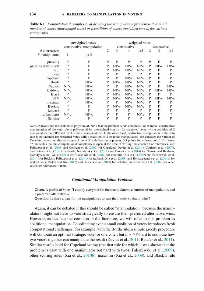
134 6 barriers to manipulation in voting
Table 6.1. Computational complexity of deciding the manipulation problem with a smallnumber of voters (unweighted votes) or a coalition of voters (weighted votes), for variousvoting rules
unweighted votes weighted votesconstructive manipulation constructive destructive
# alternatives 2 3 4 �5 2 3 �4# manipulators 1 � 2
plurality P P P P P P P P Pplurality with runoff P P P NP-c NP-c NP-c P NP-c NP-c
veto P P P NP-c NP-c NP-c P P Pcup P P P P P P P P P
Copeland P P P P NP-c NP-c P P PBorda P NP-c P NP-c NP-c NP-c P P P
Nanson NP-c NP-c P P NP-c NP-c P P NP-cBaldwin NP-c NP-c P NP-c NP-c NP-c P NP-c NP-c
Black P NP-c P NP-c NP-c NP-c P P PSTV NP-c NP-c P NP-c NP-c NP-c P NP-c NP-c
maximin P NP-c P P NP-c NP-c P P PBucklin P P P NP-c NP-c NP-c P P Pfallback P P P P P P P P P
ranked pairs NP-c NP-c P P P NP-c P P ?Schulze P P P P P P P P P
Note: P means that the problem is polynomial, NP-c that the problem is NP-complete. For example, constructivemanipulation of the veto rule is polynomial for unweighted votes or for weighted votes with a coalition of 2manipulators, but NP-hard for 3 or more manipulators. On the other hand, destructive manipulation of the vetorule is polynomial for weighted votes with a coalition of 2 or more manipulators. We consider the variant ofCopeland where an alternative gets 1 point if it defeats an opponent, 0.5 points for a draw, and 0 if it loses.“?” indicates that the computational complexity is open at the time of writing this chapter. For references, see:Faliszewski et al. (2008) and Conitzer et al. (2007) for Copeland; Davies et al. (2011), Conitzer et al. (2007),and Betzler et al. (2011) for Borda; Narodytska et al. (2011) and Davies et al. (2014) for Nanson and Baldwin;Narodytska and Walsh (2013) for Black; Xia et al. (2009) for maximin; Xia et al. (2009) and Faliszewski et al.(2014) for Bucklin; Faliszewski et al. (2014) for fallback; Xia et al. (2009) and Hemaspaandra et al. (2014c) forranked pairs; Parkes and Xia (2012) and Gaspers et al. (2013) for Schulze; and Conitzer et al. (2007) for otherresults or references to them.
Coalitional Manipulation Problem
Given. A profile of votes � cast by everyone but the manipulators, a number of manipulators, anda preferred alternative a.Question. Is there a way for the manipulators to cast their votes so that a wins?
Again, it can be debated if this should be called “manipulation” because the manip-ulators might not have to vote strategically to ensure their preferred alternative wins.However, as has become common in the literature, we will refer to this problem ascoalitional manipulation. Coordinating even a small coalition of voters introduces freshcomputational challenges. For example, with the Borda rule, a simple greedy procedurewill compute an optimal strategic vote for one voter, but it is NP-hard to compute howtwo voters together can manipulate the result (Davies et al., 2011; Betzler et al., 2011).Similar results hold for Copeland voting (the first rule for which it was shown that theproblem is easy with one manipulator but hard with two) (Faliszewski et al., 2008),other scoring rules (Xia et al., 2010b), maximin (Xia et al., 2009), and Black’s rule
6 .4 computational hardness as a barrier to manipulation 135
(Narodytska and Walsh, 2013). Intriguingly, in all these cases, it requires only twomanipulators to make manipulation hard. Black’s rule is the voting rule that elects theCondorcet winner if it exists, and otherwise the Borda winner.
One criticism that can be made about the complexity results considered so far is thatthey require the number of alternatives to grow in an unbounded fashion. If the numberof alternatives is held constant, then a single manipulator would have only a constantnumber (m!) of votes to consider. Even for a coalition of n′ manipulators, if the rule isanonymous, then the total number of joint votes for the coalition is the number of waysn′ indistinguishable balls (voters) can be placed into m! urns (possible votes), whichis(n′+m!−1
m!−1
), which is polynomial in n′. Hence, as long as there is a polynomial-time
algorithm for executing the rule, a manipulation (if one exists) can be computed inpolynomial time when the number of alternatives is constant. However, this argumentfundamentally relies on the voters being indistinguishable, which is not the case whenvoters have weights.
6.4.3 Weighted Votes
Weighted votes occur in a number of real-world settings (e.g., shareholder elections andvarious parliaments). Weights are typically integers and a vote of weight k can be seenas k identical and unweighted votes. It turns out that with weighted votes, we encountercomplexity in manipulation problems even with a small number of alternatives. Weconsider the following decision problem for weighted votes.
Coalitional Weighted Manipulation Problem
Given. A profile of weighted votes � cast by everyone but a coalition of manipulators, a weightfor each of the manipulators, and a preferred alternative a.Question. Is there a way for the manipulators to cast their votes so that a wins?
There is again a destructive variant of this problem where the coalition wants a givenalternative not to win.
With two alternatives, most common voting rules degenerate to majority voting. Inaddition, by May’s Theorem, this is the only voting rule over two alternatives that isanonymous, neutral, and positively responsive. With majority voting, the manipulators’best action even when their votes are weighted is always to vote for the alternative thatthey wish to win. With three or more alternatives, however, computing a manipulationcan be computationally hard, provided we have a coalition of manipulators (whose sizeis allowed to increase) and votes that are weighted. For example, computing how tomanipulate the veto (aka. antiplurality) rule12 is polynomial with unweighted votes butNP-complete with weighted votes and just 3 alternatives (Conitzer et al., 2007). Someintuition for this result is as follows. The manipulators could find themselves in thesituation where, after counting the nonmanipulators’ votes, two alternatives (b and c)
12 Recall that under the veto rule, the winner is the alternative that is ranked last in the fewest votes. Equivalently,it is the positional scoring rule in which the bottom rank receives 0 points and all other ranks receive 1 point.
136 6 barriers to manipulation in voting
are tied for the lead (i.e., they have been vetoed the least), but the third alternative (a)is the one that the manipulators want to win. Clearly the manipulators do not want toveto a. To make a win, however, they may need to divide their total veto weight veryevenly between b and c, so that a comes out just barely ahead of each of them. Thus,the manipulators face the problem of partitioning a set of integers (their weights) intotwo subsets (vetoing b or vetoing c) so that each subset has the same weight—and thisis an NP-complete problem. This intuition can be turned into a formal NP-hardnessreduction as follows.
Theorem 6.5. The coalitional weighted manipulation problem is NP-complete underthe veto rule, even with only three alternatives.
Proof. The problem is in NP because a profile of votes for the manipulators willserve as a certificate (because the veto rule is computationally easy to execute). Toprove NP-hardness, we reduce from the PARTITION problem, in which we are givena set of integers w1, . . . , wn′ with
∑n′i=1 wi = W (where W is even) and are asked
whether there exists a subset S ⊆ {1, . . . , n′} such that∑
i∈S wi = W/2. We reducethis problem to the coalitional weighted manipulation problem under the veto rulewith three alternatives, as follows. Let a, b, and c be the alternatives, where a is thealternative that the manipulators would like to win. Create one nonmanipulator votewith weight W − 1 that ranks a last. Furthermore, for each i ∈ {1, . . . , n′}, create amanipulator (the ith manipulator) with weight 2wi .
We now show that the manipulators can succeed in this instance if and only if theoriginal partition instance has a solution. If the partition instance has a solution S, thenlet the manipulators in S rank b last, and let the ones outside S rank c last. Then, a wins,appearing in last place only for W − 1 of the weight, whereas b and c each appear inlast place for
∑i∈S 2wi = 2W/2 = W of the weight.
Now suppose that the partition instance has no solution. This implies that for eachsubset S ⊆ {1, . . . , n′}, either
∑i∈S wi � W/2 − 1 or
∑i /∈S wi � W/2 − 1 (due to the
integrality of the wi and W/2). Then, for any profile of votes for the manipulators, let S
be the set of manipulators that rank b last. Then, we have either∑
i∈S 2wi � W − 2 <
W − 1, so that b ranks ahead of a, or∑
i /∈S 2wi � W − 2 < W − 1, so that c ranksahead of a. So the manipulators cannot make a win.
Note that the reduction is set up in such a way that a cannot end up tied for the win,so it does not matter how ties are handled. On the other hand, note that this is onlya weak NP-hardness result because the reduction is from PARTITION. Indeed, wecan compute a manipulation for a coalition of voters using dynamic programming inpseudopolynomial time—that is, in polynomial time when the weights are representedin unary (or equivalently, when the weights are small). Similar (though often moreinvolved) reductions can be given for many other rules. In fact, a dichotomy resultholds for positional scoring rules in general: every scoring rule that is not isomorphicto plurality is NP-hard to manipulate with three or more alternatives and weightedvotes (Hemaspaandra and Hemaspaandra, 2007; Procaccia and Rosenschein, 2007b;Conitzer et al., 2007).

6 .4 computational hardness as a barrier to manipulation 137
6.4.4 Tie-Breaking
For complexity-of-manipulation results like these, it is important to specify preciselyhow ties are broken. This perhaps should not be surprising, because a single manipulatorcan only change the result if the election is close to being tied. A common assumptionis that we break ties in favor of the manipulator. That is, we suppose that the preferredalternative wins if it is among the set of co-winners. This is usually justified on thegrounds that if ties are broken, say, at random, then this corresponds to increasingthe probability that the given alternative wins. However, the choice of the tie-breakingprocedure is not a minor detail. It can actually change the computational complexityof computing a manipulation. We can get different results if we break ties against themanipulator (that is, we suppose that the manipulator’s preferred alternative wins onlyif it is the unique winner).
The importance of tie-breaking can be seen in the earliest literature on computa-tional social choice. Recall that Bartholdi et al. (1989a) proved that a single agentcan manipulate the result of a Copeland election (with “straightforward” tie-breakingschemes) in polynomial time using their greedy algorithm, but when the second-ordertie-breaking rule is added manipulation becomes NP-hard.
Faliszewski et al. (2008) proved that for Copeland voting, changing the way thatpairwise ties (two alternatives that are each ranked above the other equally often) arehandled can change the computational complexity of manipulation. For example, withweighted votes and three alternatives, if ties result in a score of 0, then it is NP-hardfor a coalition to compute a manipulation that makes a given alternative the uniquewinner of the election, but this problem becomes solvable in polynomial time if tiesare given any other score. (Note that this is an “internal” form of tie-breaking, ratherthan tie-breaking between multiple winners at the end of applying an irresolute rule.)Also, if instead the manipulators seek to make that alternative just one of the winners,then the problem is solvable in polynomial time when a tie results in a score of 1, butNP-hard if ties are given any other score.
To study tie-breaking at random in more detail, Obraztsova et al. (2011) set up amodel where the manipulators have utilities over the alternatives and the goal is toincrease the expected utility of the result. All scoring rules, as well as Bucklin andplurality with runoff, can be manipulated in polynomial time in such a situation. Onthe other hand, Copeland, maximin, STV and ranked pairs are NP-hard to manipulatein this case (Obraztsova and Elkind, 2011).
Another method to deal with ties is to select a vote at random and select the highest-ranked of the tied alternatives from this vote (Tideman, 1987).13 Aziz et al. (2013f)show that, in general, there is no connection between the complexity of computing amanipulating vote when tie-breaking with a random alternative or with a random vote.However, for common rules like k-approval, Borda, and Bucklin, the computationalcomplexity increases from polynomial to NP-hard when tie-breaking with a randomvote rather than at random among the co-winners. For other rules like plurality, veto, andplurality with runoff, it remains possible to compute a manipulating vote in polynomial
13 For more on tiebreaking schemes in computational social choice, see Freeman et al. (2015).
138 6 barriers to manipulation in voting
time. Finally, for rules like STV, computing a manipulation is NP-hard irrespective ofthe tie-breaking method as it is possible to prove NP-hardness with a class of electionsin which there are never any ties.
6.4.5 Incomplete Information
So far, we have assumed that the manipulator has complete knowledge of the othervotes. This is a strong assumption that, extreme circumstances aside, is at best a roughapproximation of the truth. It is often defended on the grounds that if it is NP-hard tocompute a manipulation with complete information then it must remain so when wehave probabilistic information about the nonmanipulators’ votes (Conitzer et al., 2007).There has, however, been some work relaxing this assumption. For example, Conitzeret al. (2011a) consider the complexity of computing manipulations given only partialinformation about the nonmanipulators’ votes. Given such partial information, theyconsider whether the manipulator has a dominating nontruthful vote that makes thewinner always at least as preferable as, and sometimes more preferable than, thealternative that would win if the manipulator voted sincerely. This was further studiedby Reijngoud and Endriss (2012).
6.4.6 Building in Hardness
Once we accept hardness of manipulation as a desirable property of voting rules, itbecomes an interesting question whether we can engineer voting rules to be morecomputationally complex to manipulate. One general construction is to “hybridize”together two or more existing voting rules. For example, we might add one eliminationpre-round to the election, in which alternatives are paired off and only the one preferredby more voters goes through (Conitzer and Sandholm, 2003). This generates a newvoting rule that is often computationally hard to manipulate. In fact, the problemof computing a manipulation can now move to complexity classes higher than NPdepending on when the schedule of the pre-round is announced. Such hybrid votingrules also inherit some (but not all) of the properties of the voting rules from which theyare constructed. For example, if the initial rule is Condorcet consistent, then adding apre-round preserves Condorcet consistency.
Other types of voting rules can be hybridized together. For example, we can constructa hybrid of the Borda and Copeland rules in which we run two rounds of Borda,eliminating the lowest-scoring alternative each time, and then apply the Copeland ruleto the remaining alternatives. Such hybrids are often resistant to manipulation. Forexample, many hybrids of STV and of Borda are NP-hard to manipulate (Elkind andLipmaa, 2005). More generally, voting rules that have multiple stages successivelyeliminating alternatives tend to be more computationally difficult to manipulate thanone-stage rules (Coleman and Teague, 2007; Narodytska et al., 2011; Davies et al.,2012; Walsh and Xia, 2012).
Another way to combine together two or more voting rules is to use some aspectof the particular election (the votes, or the names of the alternatives) to pick whichvoting rule is used to compute the winner. For example, suppose we have a list of k
different voting rules. If all the alternatives’ names (viewed as natural numbers) are
6 .5 can manipulation be hard most of the time? 139
congruent, modulo k, to i then we use the ith voting rule, otherwise we use the defaultlast rule. Such a form of hybridization gives elections which are often computationallydifficult to manipulate (Hemaspaandra et al., 2009). Another possibility is to just leaveit ambiguous which of the voting rules will be used; Elkind and Erdelyi (2012) havestudied how hard it is for the manipulators to select their votes so that they succeed forany of a given set of rules. Finally, another possibility is that we have a runoff betweenthe winners of two voting rules. This also often makes manipulations more difficult tocompute (Narodytska et al., 2012).
6.5 Can Manipulation Be Hard Most of the Time?
NP-hardness is a worst-case notion. For NP-hard manipulation problems, supposingP �= NP, any manipulation algorithm will face some families of instances on which itdoes not scale polynomially. But it is not at all clear that these are the instances thatmanipulators would need to solve in practice. They may be pathological. Hence, it ispossible that these NP-hardness results lull us into a false sense of security regardingthe manipulability of our voting rules. A much better type of result would be that themanipulation problem is usually hard. Is such a result feasible, and what exactly does“usually” mean here? To investigate this, it is helpful to first consider some actualmanipulation algorithms for voting rules that are NP-hard to manipulate.
6.5.1 Some Algorithms for NP-Hard Manipulation Problems
Assuming P �= NP, a manipulation algorithm for a voting rule that is NP-hard tomanipulate can only hope to either (1) succeed on all instances and require more thanpolynomial time in the worst case, but still scale “reasonably,” particularly on “typical”instances; or (2) run in polynomial time and succeed on many, but not all, instances.
For instance, under the STV rule, Coleman and Teague (2007) give a simple enu-merative method for a coalition of k unweighted voters to compute a manipulation,which runs in O(m!(n + mk)) time (where n is the number of voters voting and m isthe number of alternatives). For a single manipulator, Conitzer et al. (2007) give anO(n1.62m) time recursive algorithm to compute the set of alternatives that can win anSTV election.
Such algorithms have been shown to perform well in practice. For example, Colemanand Teague (2007) showed experimentally that only a small coalition is needed tochange the elimination order of the STV rule in many cases. As a second example,Walsh (2010) showed that the Conitzer et al. (2007) algorithm could often quicklycompute manipulations of the STV rule even with hundreds of alternatives. Walsh(2009, 2011b) also empirically studied the computational cost of manipulating the vetorule by a coalition of weighted voters. Except in rather artificial and “hung” elections,it was easy to find manipulations or prove that none exist.
An algorithm designed for the manipulation of one specific rule, however effectiveit may be, may just be exploiting an idiosyncratic property of that particular rule. Itmay well be the case that other desirable rules do not have this property and are, in fact,“usually” hard to manipulate. One approach to addressing this criticism is to design
140 6 barriers to manipulation in voting
manipulation algorithms that are not specific to one voting rule. Such algorithms, tothe extent that they avoid exhaustive search, are heuristic in nature and do not alwayssucceed. This category of algorithms includes some of the earliest work providingtechnical results that cast doubt on whether worst-case hardness of manipulation hasany significant implications for the “typical” case. Procaccia and Rosenschein (2007b)provide a greedy algorithm for rules based on a score, in which the manipulatorscreate their votes in sequence, at each point ranking their preferred alternative firstand the remaining alternatives in increasing order of their current score. Conitzer andSandholm (2006) provide an algorithm that attempts to find two possible winners,by first choosing an arbitrary vote profile for the manipulators to find one possiblewinner a1, and then, for every remaining alternative a, choosing a vote profile for themanipulators where everyone ranks a first and a1 last. It is argued (and supported bysimulations) that usually, if the manipulators are pivotal (have a possibility of changingthe outcome of the election) at all, then they can only make two alternatives win. Forinstances where this is so, and where the voting rule satisfies a weak monotonicityproperty, the algorithm can be proved to find all alternatives that the manipulators canmake win.
All these empirical results suggest that we need to treat results about the NP-hardnessof manipulation with some care. Voters may still be able to compute a manipulationsuccessfully using rather simple and direct methods. The theoretically inclined reader,however, may feel dissatisfied with these types of results. Beyond getting intuition fromsimulations, can we actually prove that voting rules remain vulnerable to manipulationin the typical case? In what follows we discuss some of the approaches that researchershave taken to answer this question in the affirmative.
6.5.2 Approximation Methods
For almost all voting rules, we can easily make any alternative win provided wehave enough manipulators; the hardness results are merely due to a limited supplyof manipulators. With this in mind, we can consider manipulation as an optimizationproblem, where we try to minimize the number of manipulators required to achieve agiven outcome. One option is to use approximation methods to tackle such optimizationproblems.14
For example, Zuckerman et al. (2009) consider a variant of the algorithm by Pro-caccia and Rosenschein (2007b) (presented above) to compute manipulations of theBorda rule. Again, the algorithm constructs the vote of each manipulator in turn. Thealternative that the manipulators wish to win is put in first place, and the remainingalternatives are placed in the manipulator’s vote in increasing order of their currentBorda scores. The method continues constructing manipulating votes until the desiredalternative wins. A rather long and intricate argument shows that this method requiresat most one additional manipulator relative to the optimal solution. Based on a con-nection to a scheduling problem, Xia et al. (2010b) provide an algorithm that works
14 Another notion of approximation in manipulation problems is to approximately maximize an alternative’sincrease in score, given a fixed set of manipulators (Brelsford et al., 2008). Theorem 4 in that paper relates thatnotion of approximability to the one discussed here.

6 .5 can manipulation be hard most of the time? 141
for all positional scoring rules, though it may require as many as m − 2 additionalmanipulators.
6.5.3 Frequency of Manipulability
Again, whether the manipulators can achieve the result they want depends in large parton their number. We may then wonder whether, given an instance of the coalitionalmanipulation problem, we can quickly eyeball whether the manipulators are likelyto be successful, purely based on the size of their coalition relative to the size of theelectorate. It turns out that this is indeed the case. Building on earlier work by Procacciaand Rosenschein (2007a),15 Xia and Conitzer (2008a) showed that for an extremelylarge class16 of voting rules called generalized scoring rules, under some assumptionson the distribution of votes, if the number of manipulators is O(np) for p < 1/2, theprobability that a random profile is manipulable goes to zero; whereas if it is �(np) forp > 1/2, it goes to one. This leaves the knife-edge case of p = 1/2, which has beenstudied both experimentally (Walsh, 2009) and analytically (Mossel et al., 2013).
Another line of research along these lines proves quantitative versions of theGibbard-Satterthwaite impossibility result. Here, the idea is not to be satisfied witha statement that says that somewhere in the space of all possible profiles, there exists amanipulable one; rather, these results state that, under Gibbard-Satterthwaite-like con-ditions, a randomly chosen profile has a significant probability of being manipulable.After a sequence of earlier partial results along this line (Friedgut et al., 2008; Dobzin-ski and Procaccia, 2008; Xia and Conitzer, 2008b; Isaksson et al., 2012), Mossel andRacz (2012) seem to have achieved the gold standard. They prove that under a votingrule with 3 or more alternatives that is ε-far away from the set of nonmanipulablerules,17 a randomly chosen profile has a probability of being manipulable that is atleast inverse polynomial in n, m, and 1/ε.
6.5.4 Restricted Preferences
Finally, it is important to realize that it is unrealistic to assume that profiles of votesare drawn uniformly at random; generally, the voters’ preferences over the alternativesare quite structured. For example, the profile may be single-peaked. How does thisaffect the complexity of the manipulation problem? Several papers have addressed thisquestion, showing that this restriction often, but not always, makes the manipulationproblem easier (Walsh, 2007; Faliszewski et al., 2009e; Brandt et al., 2010a). While itmay seem odd in this context to focus on single-peaked preferences—for which, afterall, a desirable strategyproof voting rule is available in the form of the median voterrule18 —these results nevertheless provide important insight into how restricting thespace of profiles can cause complexity barriers to manipulation to fall apart.
15 See also Slinko (2004) and Pritchard and Wilson (2009).16 Xia and Conitzer (2009) characterize this class as those rules that are anonymous and finitely locally consistent.17 Here, the distance between two rules is the fraction of inputs on which they differ.18 Moreover, under some assumptions on strategic behavior by the voters and/or candidates, even rules such as
plurality and STV end up returning the same winner as the median voter rule when preferences are single-peaked(Brill and Conitzer, 2015).
142 6 barriers to manipulation in voting
6.6 Fully Game-Theoretic Models
The computational problems studied in this chapter so far all make some major sim-plifying assumptions. In most cases it is assumed that the votes of the other voters areknown exactly; even when this is not assumed, the other voters are not modeled asstrategic agents. If we do model them this way, this leads us into fully game-theoreticmodels, and indeed these have received some attention in the computational socialchoice community.
To make sense of this, a first issue that needs to be addressed is the staggeringmultiplicity of equilibria in most voting scenarios.19 Often, most profiles will not allowany single individual to change the outcome, and all of these profiles are Nash equilibriaas an immediate consequence. Many of these profiles will have voters vote in waysthat make no sense with respect to their true preferences. Based on this observation, wemay be able to rule out many of these equilibria—for example, we might require votersnot to play weakly dominated strategies.20 However, other issues are more difficult toaddress. For example, in a plurality election, any two of the alternatives might be castin a “front-runner” role, resulting in an equilibrium where everyone votes for one ofthese two, because to do otherwise would be to waste one’s vote. This also illustratesthat there will be many alternatives that win in some equilibrium.21
As it turns out, these issues are avoided when the voters, instead of voting simul-taneously, vote in sequence, so that each voter has full knowledge of all the previousvotes. If we additionally assume that all the preferences are common knowledge (aswell as the order in which the voters vote, and the voting rule used), and all prefer-ences are strict, then there is a unique alternative that wins in subgame-perfect Nashequilibrium.22 This can be proved by induction on the number of voters, roughly asfollows. Suppose it is true for n − 1 voters. Then, in the case of n voters, consider thefirst voter. For every vote that she might cast, she can, by the induction assumption,determine the alternative that will win in equilibrium from that point on. From all theseoptions, she will then choose the one that ranks highest in her own preferences. (Theremay be multiple votes for the first voter that achieve this, so the equilibrium votesare not unique.) This raises several interesting questions. First of all, will this resultin good outcomes? Of course, it is tricky to give a general definition of what “good”means in this context. As it turns out, though, for many rules, there exist profiles ofpreferences that, in equilibrium, result in outcomes that are quite unambiguously bad.Specifically, Xia and Conitzer (2010c) show that this is the case for rules with a lowdomination index, which indicates how many more than half of the voters are needed
19 Recall that, given the voters’ true preferences, a Nash equilibrium consists of a profile of votes such thatno individual voter can obtain an outcome she prefers to the current one by unilaterally changing hervote.
20 Recall that one strategy weakly dominates another if the former always delivers at least as good a result for theagent, and in some cases a strictly better one.
21 A recent article investigates what game structures can emerge when multiple voters are considering strategicallychanging their votes (Elkind et al., 2014b).
22 Recall that in a subgame-perfect Nash equilibrium, the strategies constitute a Nash equilibrium in everysubgame. In our case, when a subset of the voters has cast specific votes, the remainder of the voting gameconstitutes a subgame.
6 .6 fully game-theoretic models 143
to force the outcome.23 Some counterintuitive examples for the plurality rule are alsogiven by Desmedt and Elkind (2010).
Another question is whether these equilibria can be efficiently computed. A naturalapproach is to use a dynamic programming algorithm corresponding to the backwardinduction process in game theory, as follows. First compute what the last voter woulddo for every situation in which she might be placed; then compute what the second-to-last voter would do for every situation in which she might be placed (which is nowpossible because it is known at this point how the last voter would respond to anyvote that the second-to-last voter might cast); and so on. This algorithm is correct,but its runtime depends on the number of possible “situations.” What is a “situation,”anyway? One might interpret this as the entire partial profile of votes cast so far (i.e.,the node in the extensive form of the game), but this will scale very poorly. It is alsooverkill: for example, for a positional scoring rule, all that is needed is the total scoresof the alternatives so far, not the precise votes that led to this score. More generally,the amount of information necessary to summarize the votes of a subelectorate isknown as the compilation complexity of a voting rule (Chevaleyre et al., 2009; Xiaand Conitzer, 2010b). Xia and Conitzer (2010c) exploit the connection to this conceptto obtain algorithms for solving the game that, while still exponential, scale muchbetter than the naıve approach. (Desmedt and Elkind (2010) give a similar algorithmfor plurality.) Intriguingly, from simulations performed by Xia and Conitzer (2010c),the game-theoretic outcomes on random profiles do not look as bad as the worst-caseresults above might suggest. The exact complexity of the computational problem is notknown; it may be PSPACE-complete.
Still, is there nothing substantial that we can say about the equilibria of votinggames in which voters vote simultaneously? In fact, we can, if we are willing to makesome further assumptions about voters’ preferences in voting. One natural assumptionis that voters are truth-biased (Meir et al., 2010). This can be interpreted as follows:voters derive most of their utility from the outcome of the election, but they alsoderive a small amount of utility from voting truthfully. Hence, if it makes no differenceto the outcome, voters slightly prefer to tell the truth. Thompson et al. (2013) showexperimentally that for the plurality rule this dramatically reduces the set of equilibria.(They also study Bayes-Nash equilibria of games in which voters are not sure abouteach other’s preferences.) Obraztsova et al. (2013) study this model from a theoreticalperspective, again under the plurality rule.24 Another direction is to substitute the slightpreference for voting truthfully with a slight preference for abstaining (Desmedt andElkind, 2010). Yet another direction is to add dynamics where voters start at someinitial profile and iteratively update their vote to make themselves better off, until thisprocess converges (Meir et al., 2010; Lev and Rosenschein, 2012; Reyhani and Wilson,2012; Rabinovich et al., 2014).
23 A similar negative result is given by Xia et al. (2011a) in a different context, where multiple related binarydecisions must be made and these issues are voted on in sequence (but with all the voters voting at the sametime on each issue). For more on voting in such combinatorial domains, please see Chapter 9.
24 They also consider strong Nash equilibria, in which no subset of the agents can deviate in a way that makesthem all better off, and draw a connection to Condorcet winners. More about the relationship between strongequilibrium and Condorcet winners can be found in papers by Sertel and Sanver (2004), Messner and Polborn(2007), and Brill and Conitzer (2015).
144 6 barriers to manipulation in voting
The above approaches all rely on noncooperative game theory. However, as we havealready seen, it is natural to think about coalitions of voters coordinating their actions.Doing so in a game-theoretic framework is tricky, because the voters in a coalition maynot all have the same preferences. This leads us to cooperative (or coalitional) gametheory. A common solution concept there is that of the core, which is the set of alloutcomes such that no coalition of agents could break off in a way that would make allof its members happier. In the context of elections, when a group of agents deviates,how happy this makes them depends on how the agents outside of the coalition endup voting. For example, will the agents outside the coalition be able to react to thevotes of the coalition, or vice versa? These modeling choices correspond to the notionsof the α-core and the β-core. The computational complexity of these concepts in thecontext of elections is studied by Zuckerman et al. (2011). Bachrach et al. (2011) studythe complexity of problems in cooperative game theory models of manipulation wherepayments are possible.
6.6.1 Other Topics
So far, we have supposed that the manipulating coalition can communicate and coordi-nate perfectly. In practice, this may be optimistic. For example, if the coalition is large,then it may be difficult for the coalition to communicate, as well as to ensure everyonevotes appropriately. To address this, Slinko and White (2008) propose a more restrictedmodel of strategic voting in which a single coalition member broadcasts a strategicvote and every member of the coalition either casts this vote or votes sincerely. In sucha situation, a safe strategic vote is a broadcast vote that never results in an undesirableoutcome, however many or few of the coalition follow it. The Gibbard-SatterthwaiteTheorem extends to this notion of manipulation. Polynomial-time algorithms for com-puting a safe strategic vote have been given for k-approval, Bucklin, and Borda (Hazonand Elkind, 2010; Ianovski et al., 2011).
Another type of manipulation is for a single agent to vote more than once. This isoften a concern in elections run in highly anonymous environments, such as Internetvoting. A rule is said to be false-name-proof (Yokoo et al., 2004) if there is never anincentive for a voter to cast more than one vote. Conitzer (2008) gives a characterizationof false-name-proof rules similar in spirit to the characterization of strategyproof rulesby Gibbard (1977) that, perhaps unsurprisingly, is even more negative. Unlike inthe case of strategyproofness, under the constraint of false-name-proofness, even therestriction of single-peaked preferences does not allow very appealing rules (Todoet al., 2011).
6.7 Conclusions
Besides being of interest in their own right, the computational manipulation problemsdiscussed in this chapter are also important because of their implications for other,closely related problems in computational social choice. For example, the constructivemanipulation problem is a special case of the possible winner problem, which asks,given a profile of partial votes and a given alternative, whether it is possible to complete
acknowledgments 145
the profile in such a way that that alternative wins. Similarly, the destructive manipula-tion problem is a special case of the necessary winner problem. For detailed analysis ofthe complexity of these problems, see, for example, Konczak and Lang (2005), Walsh(2007), Betzler and Dorn (2010), Xia and Conitzer (2011a), and Baumeister and Rothe(2012). The necessary winner problem, in turn, is important in settings in which weincrementally elicit voters’ rankings rather than collecting them all at once. In thisproblem, we would like to be able to compute when we have elicited enough informa-tion to announce the winner (Conitzer and Sandholm, 2002). For further discussion ofall of this, see also Chapter 10. There are also relations to control and bribery problems,which will be discussed in Chapter 7.
Acknowledgments
We thank Felix Brandt, Piotr Faliszewski, Jerome Lang, Ariel Procaccia, ArkadiiSlinko, and Bill Zwicker for very detailed and helpful comments on earlier versions ofthis chapter. Conitzer thanks NSF and ARO for support under grants CCF-1101659,IIS-0953756, CCF-1337215, W911NF-12-1-0550, and W911NF-11-1-0332. Walsh issupported by the Department of Communications and the Australian Research Councilthrough the ICT Centre of Excellence Program, AOARD grant FA2386-12-1-4056, andthe Federal Ministry for Education and Research through the Alexander von HumboldtFoundation.

CHAPTER 7
Control and Bribery in Voting
Piotr Faliszewski and Jorg Rothe
7.1 Introduction
In this chapter we study control and bribery, two families of problems modeling variousways of manipulating elections. Briefly put, control problems model situations wheresome entity, usually referred to as the chair or the election organizer, has some abilityto affect the election structure. For example, the chair might be able to encourage newcandidates to join the election, or might be able to prevent some voters from casting theirvotes. On the other hand, bribery models situations where the structure of the electionstays intact (we have the same candidates and the same voters), but some outside agentpays the voters to change their votes. Naturally, such manipulative actions, dishonestlyskewing election results, are undesirable. Thus it is interesting to know if there are so-called complexity shields against these attacks (see also Chapter 6 on manipulation and,relatedly, Section 4.3.3 in the book chapter by Baumeister and Rothe (2015)). That is,it is interesting to know the computational complexity of recognizing whether variousforms of such attacks are possible or not. However, there are also other interpretationsof control and bribery, many of them quite positive.
In this chapter we survey results on the complexity of control and bribery in elec-tions, providing an overview of the specific problems studied, sketching sample proofs,and reviewing some approaches to dealing with the computational hardness of thesecontrol and bribery problems (see also Sections 4.3.4 and 4.3.5 in the book chapterby Baumeister and Rothe (2015)). Seeking ways of dealing with the computationalhardness of control and bribery may seem surprising at first. However, on one hand,if we interpret control and bribery as modeling attacks on elections, then we wouldlike to know the limitations of our complexity shields. On the other hand, if we takeother interpretations of control and bribery, then we simply would like to know how tosolve these problems. We survey some classical results on control in Section 7.3,on bribery in Section 7.4, and then briefly discuss their various applications inSection 7.5.
146

7 .2 preliminaries 147
Table 7.1. Three types of preference profiles required by different voting rules
(a) A Borda electionpoints: 5 4 3 2 1 0
voter 1: a c b f e dvoter 2: b a f c e dvoter 3: c d b a f evoter 4: e d b f c avoter 5: e d c b f a
winner: b with score 16
(b) An approval electiona b c d e f
voter 1: (1, 0, 0, 0, 0, 0)voter 2: (1, 1, 0, 0, 0, 0)voter 3: (1, 1, 1, 1, 0, 0)voter 4: (0, 0, 0, 1, 1, 0)voter 5: (0, 0, 0, 0, 1, 0)
AV score: 3 2 1 2 2 0
(c) A fallback electionlevel: 1 2 3 4
voter 1: avoter 2: b avoter 3: c d b avoter 4: e dvoter 5: e
winner: a on level 4
7.2 Preliminaries
We start by recalling various voting rules, including preference-based voting rulesand (variants of) approval voting. For the former, an election (A, R) is given by a setA of m alternatives (or candidates) and a preference profile R = (�1, . . . ,�n) overA that collects n votes, each expressing a linear preference order over A. That is,letting N = {1, . . . , n} be the set of voters, �i gives voter i’s preference order of thealternatives. For example, the ranking a �1 b �1 c says that voter 1 (strictly) prefersalternative a to alternative b, and b to c. From now on we omit stating “�i” explicitlyand simply rank the alternatives in a vote from left (most preferred) to right (leastpreferred). That is, instead of, say, a �1 b �1 c we simply write a b c. Also, for (A, R)an election and A′ ⊆ A, we write (A′, R) to denote the election with alternativesA′ and the votes in R restricted to A′. For example, if (A, R) is the election fromTable 7.1(a) consisting of five voters who rank six alternatives and A′ = {b, c, d}, then(A′, R) = ({b, c, d}, (c b d, b c d, c d b, d b c, d c b)).
We briefly recall some voting rules, see Chapter 2 for more details. Positional scoringrules are defined by an m-alternative scoring vector σ = (σ1, σ2, . . . , σm), where the σi
are nonnegative integers with σ1 � σ2 � · · · � σm. Each alternative scores σi points foreach vote where it is ranked in the ith position, and whoever scores the most points wins.Examples are plurality voting with scoring vector (1, 0, . . . , 0), veto (aka antiplurality)with (1, . . . , 1, 0), k-approval with (1, . . . , 1, 0, . . . , 0) having a 1 in each of the firstk � m positions (note that 1-approval is plurality), k-veto, which is the same as (m − k)-approval (note that 1-veto is veto), and Borda count with (m − 1, m − 2, . . . , 0). Forexample, in the election given in Table 7.1(a), e wins under plurality; d under 2-approval; b under 3-approval; b, c, and f under veto; and b under Borda (with aBorda score of 16, whereas a, c, d, e, and f score, respectively, 11, 15, 12, 12, and 9points).
Under approval voting (or AV), proposed by Brams and Fishburn (1978, 2007),instead of using preference orders the voters specify sets of alternatives they approveof. Typically, such votes are represented as m-dimensional 0/1-vectors, where eachposition corresponds to an alternative and 1-entries mean approval of respective alter-natives. All alternatives with the most approvals win. For example, for the approvalvectors given in Table 7.1(b), a is the approval winner with a score of 3. A versionof approval voting (dubbed sincere-strategy preference-based approval voting (or SP-AV) by Erdelyi et al. (2009)) combines approval information with preference-order
148 7 control and bribery in voting
information (the voters rank the candidates that they approve of). The rule was intro-duced by Brams and Sanver (2006) and, in essence, is the same as approval, but theadditional preference-order information is used to deduce voter behavior when thecandidate set changes (we omit detailed discussion and point the reader to the originalpapers and to the survey of Baumeister et al. (2010)).
Range voting (or RV) works just as approval voting, except that entries of the vectorsunder k-range voting come from the set {0, 1, . . . , k} rather than from the set {0, 1}.Normalized range voting (or NRV) is a variant of RV that alters the votes so that thepotential impact of each vote is maximized (see, e.g., the work of Menton, 2013).
Let us now move back to rules based on preference orders and, in particular, tothose rules that are based on pairwise comparisons of alternatives. A Condorcet win-ner is an alternative that is preferred to every other alternative by a strict majority ofvotes. For example, in the election from Table 7.1(a), c is preferred to every otheralternative by three of the five voters and thus is the Condorcet winner. It is easy tosee that there is at most one Condorcet winner in an election, but it is possible thatthere is none.1 A voting rule is Condorcet-consistent if it elects the Condorcet winnerwhenever there is one. If there is no Condorcet winner in a given preference profile,many of the known Condorcet-consistent rules elect those candidates that are closest tobeing Condorcet winners, one way or another. For example, under Copelandα voting,α ∈ [0, 1], we organize a tournament among the candidates in the following way: Eachpair of candidates “plays” against each other and the one that is preferred by morevoters wins and receives a point (in case of a tie, both get α points). In the end, thecandidates with the highest number of points win. If we omit voter 1 from the electionin Table 7.1(a) then d is the unique Copelandα winner for α = 0 and α = 1/2 (with aCopelandα score of 3 if α = 0, and of 3.5 if α = 1/2), but both c and e are Copelandα
winners with a score of 5 for α = 1. Other Condorcet-consistent rules are, for exam-ple, the maximin rule (aka Simpson’s rule), ranked pairs due to Tideman (1987), orSchulze’s rule (a rule proposed by Schulze (2011), which satisfies many normativeproperties).
Other voting rules follow yet other principles, e.g., single transferable vote (STV)proceeds in stages and eliminates the “weakest” candidates until only the winnerremains. We omit the details and point the reader to Chapter 2 instead. Under Bucklinvoting we first seek the smallest value such that there is candidate ranked amongtop positions by a strict majority of the voters, and then declare as winners thosecandidates that have highest -approval scores (or, under simplified Bucklin voting,those candidates that are ranked among top positions by some majority of the voters).Fallback voting, introduced by Brams and Sanver (2009), is a rule that combinesBucklin voting with approval voting (the voters rank only the candidates they approveof and Bucklin is used; if there are no Bucklin winners—due to the fact that votersdo not have to rank all the candidates—fallback outputs the approval winners). Forexample, in the partial rankings given in Table 7.1(c), a alone reaches a strict majority
1 If one requires voting rules to always have at least one winner, Condorcet voting (which elects the Condorcetwinner whenever there is one, and otherwise no one wins) would not be a voting rule. However, we take thepoint of view that voting rules may have empty winner sets. Note that it has become a tradition to study (atleast) plurality, Condorcet, and approval on each new approach and each new idea regarding election control(see, e.g., the papers of Bartholdi et al., 1992; Hemaspaandra et al., 2007; Faliszewski et al., 2011c).
7 .3 control 149
of !5/2" + 1 = 3 votes (namely, on the fourth level) and thus is the fallback winner.However, if the first voter approved only of f instead of only of a, then no candidatewould reach a majority and fallback would output a, b, d, and e, the approval winnersof the election.
In Sections 7.3 and 7.4, we will define a large variety of decision problems, eachrelated to some specific control or bribery scenario. All these problems are membersof NP, the class of problems that can be solved in nondeterministic polynomial time,and they will be classified to be either in P or NP-complete.2 Unlike, for instance, inthe case of Kemeny, Dodgson, and Young elections (which we do not consider here,as their winner problems are not in P—see Chapters 4 and 5), the winner(s) can bedetermined efficiently for all voting systems described earlier.
7.3 Control
Every election needs to be organized, and whoever is responsible for doing so can havesome influence on the outcome of the election by changing its structure. We will referto this person, or authority, as the chair of the election, and to the way the electionstructure is changed by the chair as control type or control action. Many types of controlthat the chair might exert are conceivable. We present those that have been studied inthe literature, starting with the four most important ones.
7.3.1 Constructive Control by Adding/Deleting Candidates/Voters
Bartholdi et al. (1992) were the first to introduce electoral control and to study itin various scenarios from a computational perspective. In particular, they definedconstructive control types, where the chair’s goal in exerting some control action is tomake a given candidate p the unique winner of the resulting election.3 It is common toassume that the chair has complete knowledge of all votes.
One control action the chair might exert is to change the candidate set, either byadding some new candidates from a given set of spoiler candidates (hoping to makep’s most competitive rivals weaker relative to p), or to delete up to k candidates fromthe given election (to get rid of p’s worst rivals). For the former, Bartholdi et al.(1992) originally defined a variant that allows adding an unlimited number of spoilercandidates. To be in sync with the other control problems (e.g., control by deletingcandidates), Hemaspaandra et al. (2009) defined a variant of this problem where abound k on the number of spoiler candidates that may be added is given. We will seelater that the complexity of the resulting problems can sharply differ.
2 A problem B is NP-hard if every NP problem A reduces to B, where “reduction” always refers to a polynomial-time many-one reduction, that is, a polynomial-time function r mapping instances of A to instances of B suchthat for each x, x ∈ A ⇐⇒ r(x) ∈ B. B is NP-complete if it is NP-hard and in NP.
3 As we do here, control problems have commonly, most especially in the earlier papers on control, been studiedin their unique-winner variant. Alternatively, many papers on control consider the nonunique-winner (or co-winner, or simply winner) variant where the chair’s goal is merely to make the designated candidate a winner.The complexity of control problems is usually the same in both models, requiring only minor adjustments tothe proofs.

150 7 control and bribery in voting
Definition 7.1. Let f be a voting rule. In the Constructive-Control-by-Adding-an-Unlimited-Number-of-Candidates problem for f (f -CCAUC), we are given(a) a set A of qualified candidates, a set B of spoiler candidates, where A ∩ B = ∅,and an election (A ∪ B, R) and (b) a preferred candidate p ∈ A. We ask if we canchoose a subset B ′ ⊆ B of the spoiler candidates such that p is the unique f -winnerof the election (A ∪ B ′, R). The Constructive-Control-by-Adding-Candidatesproblem for f (f -CCAC) is defined similarly: In addition to (a) and (b) we are alsogiven (c) a bound k ∈ N, and we ask if there is a subset B ′ ⊆ B of spoiler candidatessuch that |B ′| � k and p is the unique f -winner of (A ∪ B ′, R). In the Constructive-Control-by-Deleting-Candidates problem for f (f -CCDC), we are given (a) anelection (A, R), (b) a preferred candidate p ∈ A, and (c) a bound k ∈ N. We ask if p
can be made a unique f -winner of the election resulting from (A, R) by deleting atmost k candidates.
The issue of control by changing the candidate set is very natural and, indeed, hap-pens in real-life political elections. For example, it is widely speculated that “adding”Nader to the 2000 U.S. presidential election had the effect of ensuring Bush’s victory(otherwise, Gore would have won). Similarly, there are known cases where “spoiler”candidates were added to political elections to confuse the voters (see, e.g., the NewYork Times article of Lacey (2010) for a reported example). It is also easy to imag-ine control by deleting candidates: Some of the candidates who perform poorly inpre-election polls may be forced (or persuaded) to withdraw.
Example 7.1. For a Borda-CCAUC instance, let (A ∪ B, R) be the election fromTable 7.1(a), where A = {a, b, c, d} is the set of qualified candidates and B = {e, f } isthe set of spoiler candidates. Table 7.2(a) shows the restriction (A, R) of this electionto the qualified candidates, which has the Borda winner c scoring 9 points, while theBorda scores of a, b, and d, respectively, are 4, 6, and 8. Supposing that b is the chair’sfavorite candidate, we have a yes-instance of Borda-CCAUC, since adding both spoilercandidates makes b the unique Borda winner (see Table 7.1(a)).
To turn this into a Borda-CCAC instance, we in addition need to specify an additionlimit, k. If k = 1, we have a yes-instance of the problem: Though the chair will notsucceed by adding e (which gives the election in Table 7.2(c), still won by c), adding f
(giving the election in Table 7.2(b)) will make b the unique Borda winner with a scoreof 13, while a, c, d, and e score 8, 12, 11, and 6 points.
Finally, consider again the Borda election in Table 7.1(a) with winner b, and supposethe chair, who now wants to make c win, is allowed to delete one candidate. Deletingthe current champion, b, will reach this goal. Alternatively, the chair can delete f (seeTable 7.2(c)) to turn c into the unique winner with a Borda score of 12, while the Bordascores of a, b, d, and e, respectively, are reduced to 8, 11, 9, and 10. Thus this is ayes-instance of the problem Borda-CCDC.
The chair might also change the voter set, either by encouraging further voters toparticipate (knowing that their votes will be beneficial for p), or by excluding certainvoters from the election (knowing that deleting their votes will help p). In real life,political parties often try to influence the outcome of elections by such actions (e.g.,
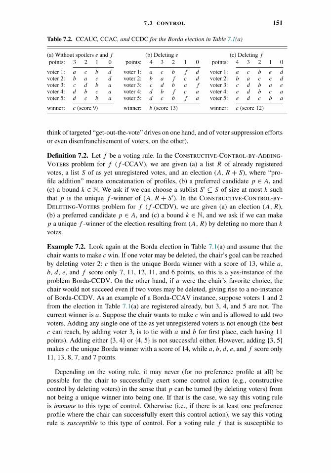
7 .3 control 151
Table 7.2. CCAUC, CCAC, and CCDC for the Borda election in Table 7.1(a)
(a) Without spoilers e and f
points: 3 2 1 0
voter 1: a c b dvoter 2: b a c dvoter 3: c d b avoter 4: d b c avoter 5: d c b a
winner: c (score 9)
(b) Deleting e
points: 4 3 2 1 0
voter 1: a c b f dvoter 2: b a f c dvoter 3: c d b a fvoter 4: d b f c avoter 5: d c b f a
winner: b (score 13)
(c) Deleting f
points: 4 3 2 1 0
voter 1: a c b e dvoter 2: b a c e dvoter 3: c d b a evoter 4: e d b c avoter 5: e d c b a
winner: c (score 12)
think of targeted “get-out-the-vote” drives on one hand, and of voter suppression effortsor even disenfranchisement of voters, on the other).
Definition 7.2. Let f be a voting rule. In the Constructive-Control-by-Adding-Voters problem for f (f -CCAV), we are given (a) a list R of already registeredvotes, a list S of as yet unregistered votes, and an election (A, R + S), where “pro-file addition” means concatenation of profiles, (b) a preferred candidate p ∈ A, and(c) a bound k ∈ N. We ask if we can choose a sublist S ′ ⊆ S of size at most k suchthat p is the unique f -winner of (A, R + S ′). In the Constructive-Control-by-Deleting-Voters problem for f (f -CCDV), we are given (a) an election (A, R),(b) a preferred candidate p ∈ A, and (c) a bound k ∈ N, and we ask if we can makep a unique f -winner of the election resulting from (A, R) by deleting no more than k
votes.
Example 7.2. Look again at the Borda election in Table 7.1(a) and assume that thechair wants to make c win. If one voter may be deleted, the chair’s goal can be reachedby deleting voter 2: c then is the unique Borda winner with a score of 13, while a,b, d, e, and f score only 7, 11, 12, 11, and 6 points, so this is a yes-instance of theproblem Borda-CCDV. On the other hand, if a were the chair’s favorite choice, thechair would not succeed even if two votes may be deleted, giving rise to a no-instanceof Borda-CCDV. As an example of a Borda-CCAV instance, suppose voters 1 and 2from the election in Table 7.1(a) are registered already, but 3, 4, and 5 are not. Thecurrent winner is a. Suppose the chair wants to make c win and is allowed to add twovoters. Adding any single one of the as yet unregistered voters is not enough (the bestc can reach, by adding voter 3, is to tie with a and b for first place, each having 11points). Adding either {3, 4} or {4, 5} is not successful either. However, adding {3, 5}makes c the unique Borda winner with a score of 14, while a, b, d, e, and f score only11, 13, 8, 7, and 7 points.
Depending on the voting rule, it may never (for no preference profile at all) bepossible for the chair to successfully exert some control action (e.g., constructivecontrol by deleting voters) in the sense that p can be turned (by deleting voters) fromnot being a unique winner into being one. If that is the case, we say this voting ruleis immune to this type of control. Otherwise (i.e., if there is at least one preferenceprofile where the chair can successfully exert this control action), we say this votingrule is susceptible to this type of control. For a voting rule f that is susceptible to
152 7 control and bribery in voting
some type of control (e.g., to constructive control by adding voters), f is said to bevulnerable (respectively, resistant) to this control type if the corresponding problem(e.g., f -CCAV) is in P (respectively, NP-hard).
Immunity results appear to be very desirable. Indeed, if a voting rule is immune to agiven type of control, then it is impossible to compromise its result by a correspondingtype of malicious action. Nonetheless, as we will soon see, immunity can also bringsome undesired side effects. First, however, let us argue that immunity for candidatecontrol is rare. This is so due to the study of strategic candidacy of Dutta et al.(2001) (see also recent work on strategic candidacy of Lang et al. (2013) and Brill andConitzer (2015)). They have considered a setting where the candidates have preferencesregarding election outcomes, and can strategically choose to join the race or not.Dutta et al. (2001) have shown that for most typical election rules there are settingswhere some candidates would prefer not to participate in the election. In effect, suchrules cannot be immune to candidate control. Nonetheless, in some rare cases (e.g.,for Condorcet and approval voting) immunity results for candidate control hold (seeTable 7.3).
For the case of voter control, immunity is not only rare, but also is utterly undesirable.Indeed, it is natural to expect that if we add sufficiently many voters with the samepreference order, then their most preferred candidate becomes a winner. Formally, thisis known as voting rule continuity (or, as the Archimedean property). Continuity saysthat if some candidate c is a winner in some election (A, R), then for every election(A, R′), there is a natural number t such that c is a winner in an election of the form(A, R′ + tR), where tR refers to a profile of t copies of profile R. See, for example,the work of Smith (1973).
The first voting rules studied with respect to control were plurality, Condorcet, andapproval voting. The following theorem summarizes some of the results obtained forthem by Bartholdi et al. (1992) and Hemaspaandra et al. (2007).
Theorem 7.3 (Bartholdi et al., 1992; Hemaspaandra et al., 2007).
1. Condorcet and approval voting are immune and plurality is resistant to constructivecontrol by adding (respectively, adding an unlimited number of) candidates.
2. Condorcet and approval voting are vulnerable and plurality is resistant to constructivecontrol by deleting candidates.
3. Condorcet and approval voting are resistant and plurality is vulnerable to constructivecontrol by both adding and deleting voters.
These immunity claims generally follow from the fact that Condorcet and approvalvoting satisfy the (“unique” version of the) Weak Axiom of Revealed Preference,which states that a unique winner p in a set A of alternatives always is also a uniquewinner among each subset A′ ⊆ A including p. Hemaspaandra et al. (2007) identifymany links (i.e., implications and equivalences) among the susceptibility/immunitystatements for the control types defined previously and to be defined in Section 7.3.2.We refrain from repeating them here but point the reader to Figure 4.16 in the book byRothe et al. (2011) for an overview.
The vulnerability claims in Theorem 7.3 follow by simple P algorithms. For example,that approval-CCDC is in P follows from this algorithm: On input ((A, R), p, k), if p

7 .3 control 153
already is the unique winner in (A, R) (which is easy to test), output “yes”; otherwise,if no more than k candidates have at least as many approvals as p, output “yes” (as p
can be made a unique winner by deleting them all), and else output “no.” By contrast,vulnerability proofs for the partitioning cases to be defined in Section 7.3.2 are oftenmuch more involved (and are omitted here).
The resistance claims in Theorem 7.3 typically follow by reductions from NP-complete problems such as Exact-Cover-by-3-Sets (X3C), which given a base setB = {b1, . . . , b3k}, k > 0, and a sequence S = (S1, . . . , Sn) of 3-element subsets of B,asks whether B can be exactly covered by k sets chosen from S . For example, to showthat approval-CCDV is NP-hard, let (B,S) be an instance of X3C. Let j = |{Si ∈S | bj ∈ Si}| for each j , 1 � j � 3k. Construct from (B,S) the election (A, R) withA = B ∪ {p} and R consisting of the following 2n voters: (1) For each i, 1 � i � n,one voter in R approves of all candidates in Si and disapproves of all other candidates;(2) there are n voters v1, . . . , vn in R such that, for each i, 1 � i � n, vi (a) approvesof p, and (b) approves of bj if and only if i � n − j . Thus, every candidate in (A, R)has exactly n approvals. If there is an exact cover for B, then deleting the k votes fromR corresponding to the exact cover turns p into the unique winner. Conversely, supposethat p can be turned into a unique approval winner by deleting at most k votes from R
(where we may assume that none of them approves of p, so only votes from group (1)have been deleted). For p to become the unique approval winner, every bj ∈ B musthave lost at least one approval. Thus, the deleted votes correspond to an exact coverfor B.
The next system to be comprehensively studied regarding control was Copelandα .
Theorem 7.4 (Faliszewski et al., 2009c). For each rational number α, 0 � α � 1,Copelandα is resistant to all types of control from Definitions 7.1 and 7.2, exceptfor α ∈ {0, 1} where Copelandα is vulnerable to constructive control by adding anunlimited number of candidates.
The most interesting point to note in Theorem 7.4 is that Copelandα-CCAUC is inP for α = 0 and α = 1, but is NP-complete for all other values of α. The vulnerabilityresults are proven by the following simple P algorithm: On input ((A ∪ B, R), p),set D1 to be the set of all b ∈ B such that the Copelandα score of p in ({b, p}, R)is 1; initialize D to be D1; and then successively delete every b from D such that theCopelandα score of p in (A ∪ D, R) is no greater than that of b. Correctness of thealgorithm follows from (1) the observation that for each D ⊆ B, whenever p is theunique Copelandα winner in (A ∪ D, R), then so is p in (A ∪ (D1 ∩ D), R), and (2) amore involved argument showing that if p is the unique winner in (A ∪ D, R) for someD ⊆ D1, yet the above algorithm computes a set D′ such that p is not a unique winnerin (A ∪ D′, R), then this leads to a contradiction. On the other hand, NP-hardnessof Copelandα-CCAUC for 0 < α < 1 follows by a reduction from the NP-completeproblem Vertex-Cover (and is omitted here).
Unlike Copelandα-CCAUC, Copelandα-CCAC is NP-complete for all (rational)values of α ∈ [0, 1]. In fact, Copelandα with 0 < α < 1 (including the original systemby Copeland (1951)) is the first family of voting rules known to be fully resistantto all types of constructive control, including those to be defined in Section 7.3.2.Other voting rules having this property have followed: SP-AV (Erdelyi et al., 2009),
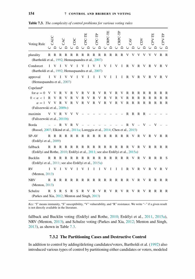
154 7 control and bribery in voting
Table 7.3. The complexity of control problems for various voting rules
Voting Rule CA
UC
CA
C
CD
C
CPC
-TE
CPC
-TP
CR
PC-T
E
CR
PC-T
P
CA
V
CD
V
CPV
-TE
CPV
-TP
C D C D C D C D C D C D C D C D C D C D C D
plurality R R R R R R R R R R R R R R V V V V V V R R
(Bartholdi et al., 1992; Hemaspaandra et al., 2007)
Condorcet I V I V V I V I V I V I V I R V R V R V R V
(Bartholdi et al., 1992; Hemaspaandra et al., 2007)
approval I V I V V I V I I I V I I I R V R V R V R V
(Hemaspaandra et al., 2007)
Copelandα
for α = 0 V V R V R V R V R V R V R V R R R R R R R R
0 < α < 1 R V R V R V R V R V R V R V R R R R R R R R
α = 1 V V R V R V R V R V R V R V R R R R R R R R
(Faliszewski et al., 2009c)
maximin V V R V V V – – – – – – – – R R R R – – – –
(Faliszewski et al., 2011b)
Borda – – R V R V – – – – – – – – R V – V – V – –
(Russel, 2007; Elkind et al., 2011a; Loreggia et al., 2014; Chen et al., 2015)
SP-AV R R R R R R R R R R R R R R R V R V R V R R
(Erdelyi et al., 2009)
fallback R R R R R R R R R R R R R R R V R V R R R R
(Erdelyi and Rothe, 2010; Erdelyi et al., 2011; see also Erdelyi et al., 2015a)
Bucklin R R R R R R R R R R R R R R R V R V R R R S
(Erdelyi et al., 2011; see also Erdelyi et al., 2015a)
RV I V I V V I V I I I V I I I R V R V R V R V
(Menton, 2013)
NRV R R R R R R R R R R R R R R R V R V R R R R
(Menton, 2013)
Schulze R S R S R S R V R V R V R V R V R V R R R R
(Parkes and Xia, 2012; Menton and Singh, 2013)
Key: “I” means immunity, “S” susceptibility, “V” vulnerability, and “R” resistance. We write “–” if a given resultis not directly available in the literature.
fallback and Bucklin voting (Erdelyi and Rothe, 2010; Erdelyi et al., 2011, 2015a),NRV (Menton, 2013), and Schulze voting (Parkes and Xia, 2012; Menton and Singh,2013), as shown in Table 7.3.
7.3.2 The Partitioning Cases and Destructive Control
In addition to control by adding/deleting candidates/voters, Bartholdi et al. (1992) alsointroduced various types of control by partitioning either candidates or voters, modeled
7 .3 control 155
by elections proceeding in two stages. While their original definitions were a bit unclearabout what happens when more than one candidate wins some first-stage pre-election,Hemaspaandra et al. (2007) defined two rules for how to handle such pre-election ties:TE (“ties eliminate”) says that whenever at least two candidates are tied for winnerin a pre-election, no candidate proceeds to the final stage from it (i.e., only uniquepre-election winners move forward); TP (“ties promote”) says that all pre-electionwinners, no matter how many, proceed forward.
Definition 7.3. Let f be a voting rule. In the Constructive-Control-by-Runoff-Partition-of-Candidates problem for f under TE or TP (f -CCRPC-TE or f -CCRPC-TP), we are given (a) an election (A, R), and (b) a preferred candidate p ∈ A.We ask if we can partition A into A1 and A2 such that p is the unique f -winner ofthe election (W1 ∪ W2, R), where Wi , i ∈ {1, 2}, is the set of those pre-election (Ai, R)winners that are promoted to the final stage according to the tie-handling rule (TEor TP). The Constructive-Control-by-Partition-of-Candidates problem for f
under TE or TP (f -CCPC-TE or f -CCPC-TP) is defined similarly, except that we askif p can be made a unique f -winner of the election (W1 ∪ A2, R) by partitioning A
into A1 and A2, i.e., there is only one pre-election (A1, R) whose winners proceed(according to the tie-handling rule, TE or TP) to the final stage to face all of A2.
Example 7.5. Let (A, R) be the Borda election in Table 7.1(a) again, and let c be thedistinguished candidate the chair wants to win. This is a yes-instance in all four cases,for both CCRPC and CCPC, each in TE and TP, as witnessed by the partition of A
into A1 = {a, f } and A2 = {b, c, d, e}. It does not matter whether we are in the TEor TP model,4 since both subelections have a unique winner: a alone wins (A1, R),and c alone wins (A2, R) (with a score of 9, while b, d, and e score only 7, 6, and8 points). For CCRPC, both subelection winners, c and a, proceed to the final stage,which c wins. For CCPC, the winner of the first subelection, a, faces all candidates ofA2 in the final stage, and as we have seen in Table 7.2(c), the unique Borda winner of({a, b, c, d, e}, R) is c, again as desired by the chair.
The analogues of f -CCRPC-TE/TP where not the candidates but the voters arepartitioned model a very basic kind of gerrymandering. (Note that it would not makesense to define voter-partition analogues of f -CCPC-TE/TP, at least not for naturalvoting systems f .5)
Definition 7.4. Let f be a voting rule. In the Constructive-Control-by-Partition-of-Voters problem for f under TE or TP (f -CCPV-TE or f -CCPV-TP), we aregiven (a) an election (A, R), and (b) a preferred candidate p ∈ A. We ask if R canbe partitioned into R1 and R2 such that p is the unique f -winner of (W1 ∪ W2, R),
4 By contrast, partitioning A into A′1 = {a, b, c} and A′
2 = {d, e, f } would reveal a difference between the twotie-handling models: Since b and c tie for winning (A′
1, R), they both proceed to the final stage in model TP(where they face e, the winner of (A′
2, R), and c wins the final stage), but b and c eliminate each other in modelTE (so e alone proceeds to the final stage and wins).
5 In such an analogue, given an election (A, R) and p ∈ A, we would partition R into R1 and R2 just as inDefinition 7.4, but there is only one pre-election, say (A, R1), whose TE/TP-winners W1 would then face allcandidates in the final stage, yet (W1 ∪ A, R) = (A, R) is just the original election.

156 7 control and bribery in voting
where Wi , i ∈ {1, 2}, is the set of those pre-election (A, Ri) winners that are promotedto the final stage according to the tie-handling rule (TE or TP).
Example 7.6. Again looking at the Borda election (A, R) in Table 7.1(a) with preferredcandidate c, the chair will succeed (in both TE and TP) by partitioning R into R1 ={1, 2, 4, 5} and R2 = {3}: b alone wins (A, R1) (with a score of 13, while a, c, d, e,and f score only 9, 10, 8, 12, and 8 points), and c alone wins (A, R2). Thus they bothproceed to the final stage where c beats b by 3 to 2.
The proofs that show the complexity of control by partitioning candidates or votersare often based on similar constructions as analogous proofs for the case of deletingcandidates or voters, but usually are more involved technically.
For each constructive control problem, there is also a destructive variant, introducedby Hemaspaandra et al. (2007), where the chair’s goal is to preclude a given candidatefrom being the unique winner of the election resulting from the chair’s control action.We denote the destructive control problems analogously, replacing the initial “C” by a“D,” as, for example, in DCDC for “destructive control by deleting candidates.” (In thisproblem, it is forbidden to delete the designated candidate p; otherwise, the problemwould be trivial.)
7.3.3 Overview and Some Other Approaches to Control
Table 7.3 summarizes the control complexity results for some prominent voting rules.In most cases we have full knowledge of the complexity of all the basic types ofcontrol, but for Borda and maximin some types of control were never studied, and forBucklin and Schulze for some types of control there are only susceptibility results inthe literature.
We already mentioned that besides Copelandα voting, 0 < α < 1, also SP-AV(Erdelyi et al., 2009), fallback and Bucklin voting (Erdelyi and Rothe, 2010; Erdelyiet al., 2011, 2015a), NRV (Menton, 2013), and Schulze voting (Parkes and Xia, 2012;Menton and Singh, 2013) are resistant to all constructive control types. Among those,Schulze has many vulnerabilities to destructive control types, but SP-AV is vulnerableto only three of them (DCAV, DCDV, and DCPV-TE), and fallback, Bucklin, andNRV even to only two (DCAV and DCDV), where the case of Bucklin-DCPV-TP isstill open. Note that SP-AV is a somewhat unnatural system (as has been discussed byBaumeister et al. (2010) in detail), due to a rule introduced by Erdelyi et al. (2009)that, to cope with certain control actions, can move the voters’ approval lines after theyhave cast their votes. It may be argued that NRV has a similar issue (though perhapsto a lesser extent), since after the voters have cast their votes (namely, their rangevoting vectors), the normalization process can change the points the alternatives willscore from the votes. Fallback’s drawback, on the other hand, is that it is a hybrid oftwo “pure” voting rules, Bucklin and approval, and requires the voters to report bothapproval vectors and rankings. All three voting systems have the disadvantage thatit is rather complicated (even though far less complicated than in Schulze voting) todetermine the winners; for example, it is hardly conceivable that many of the voters ina real-world political election would be fully aware of the effect of normalization inNRV. But this is the price to pay if we wish to have a (relatively) natural voting rule
7 .3 control 157
with P-time winner determination that is resistant to as many control actions as thesevoting rules are resistant to. On the other hand, if one is willing to accept an artificialvoting rule, Hemaspaandra et al. (2009) have shown how to combine well-known rulesto obtain ones that are resistant to all types of control. While their method producesrules that are not attractive in practice (even though they satisfy some natural normativeproperties), it suggests that indeed there might exist natural voting rules with P-timewinner determination that are resistant to all types of control considered here.
Now, let us quickly point to some related work and to other approaches to con-trol. Meir et al. (2008) study control for multiwinner voting rules. In the multiwinnersetting, we are given an election (A, R) and an integer k, and the goal is to pick a“committee” of k winners. Multiwinner voting rules can be used to choose parliaments(or other collective bodies), to choose finalists in competitions, or even within recom-mendation systems (see, e.g., the work of Lu and Boutilier (2011a) for the applicationin recommendation systems and the work of Elkind et al. (2014a) for a recent gen-eral discussion of multiwinner voting). To study control in the multiwinner setting (andanalogous approaches apply to other manipulative scenarios), Meir et al. (2008) assumethat the election chair associates some utility value with each candidate and his or hergoal is to ensure that the sum of the utilities of the candidates in the elected committeeis as high as possible. As a side effect, this approach creates a natural unification ofthe constructive and destructive cases: In the constructive case the chair would havepositive utility only for the most preferred candidate, whereas in the destructive settingthe chair would have positive, equal utilities for all the candidates except the despisedone.
Faliszewski et al. (2011b) provide a unified framework to capture “multimodecontrol attacks” that simultaneously combine various of the control actions consideredhere. Specifically, in their setting the chair can, for example, simultaneously add somecandidates and remove some voters. One of the conclusions of this work is that,typically, the complexity of such a multimode control attack is the same as that ofthe hardest basic control type involved. In particular, if a voting rule is vulnerable toseveral basic types of control, it is also vulnerable if the chair can perform these controltypes simultaneously (i.e., coordinating the attacks is easy). However, this conclusionis based on studying a number of natural voting rules and is not a general theorem(indeed, such a general theorem does not hold).
Fitzsimmons et al. (2013) study the complexity of control in the presence of manip-ulators, both in the case where the chair and the manipulators coordinate their actionsand in the case where they compete with each other. While all the related cooperativeproblems are in NP, they show that the competitive problems can be complete for thesecond and the third level of the polynomial hierarchy for suitably designed artificialvoting systems (though their complexity is much lower for many natural voting sys-tems). Another approach to unifying different types of strategic behavior is due to Xia(2012b), who proposes a general framework that is based on so-called vote operationsand can be used to express, for example, bribery and control by adding or deletingvoters. Xia (2012b) shows that if the votes are generated i.i.d. with respect to somedistribution, then, on the average, the number of vote operations (e.g., the number ofvoters that need to be added) necessary to achieve a particular effect (e.g., ensuringthat some candidate is a winner) is either zero (the effect is already achieved), or is
158 7 control and bribery in voting
proportional to the square root of the number of original voters, or is linear with respectto the number of original voters, or the effect is impossible to achieve.
Going in a somewhat different direction, Chen et al. (2014) consider control byadding candidates in a combinatorial setting, where one can add whole groups ofvoters at unit cost. They show that even for the plurality rule, for which standard votercontrol is very easy, the combinatorial setting is challenging (indeed, combinatorialcontrol by adding voters is NP-hard for plurality even in the settings where the groupsof voters to add contain at most two voters each).
Hemaspaandra et al. (2014b) established the first control-related dichotomy result,showing for which pure scoring rules CCAV is easy to solve and for which thisproblem is NP-complete (however, Faliszewski et al. (2013) study voter control inweighted elections and in the technical report version of their paper show a dichotomyresult as well). This complements similar dichotomy results of Hemaspaandra andHemaspaandra (2007) on manipulation and of Betzler and Dorn (2010) and Baumeisterand Rothe (2012) on the possible winner problem.
Some researchers investigate not only the classical complexity, but also the parame-terized complexity of control problems, with respect to such parameters as the solutionsize (e.g., “number of added voters”) or the election size (e.g., “number of candidates”);for example, see the work of Liu et al. (2009) for a discussion of plurality, Condorcet,and approval; Liu and Zhu (2010, 2013) for maximin, Copeland, Borda, Bucklin, andapproval; Betzler and Uhlmann (2009) and Faliszewski et al. (2009c) for Copelandα;Erdelyi et al. (2015a) for Bucklin and fallback; and Hemaspaandra et al. (2013b) forSchulze and ranked-pairs voting. On the other hand, Brelsford et al. (2008) study theapproximability of control, manipulation, and bribery. Faliszewski et al. (2013) discussapproximation algorithms for voter control under k-approval.
Faliszewski et al. (2011b, 2011a) and Brandt et al. (2010a) study to what extentcomplexity shields for manipulation and control disappear in elections with domainrestrictions, such as in single-peaked or nearly single-peaked electorates (see also thebook chapter by Hemaspaandra et al., 2015). Magiera and Faliszewski (2014) showsimilar results for single-crossing electorates.
Hemaspaandra et al. (2013a) compare the decision problems for manipulation,bribery, and control with their search versions and study conditions under whichsearch reduces to decision. They also notice that two destructive control types thatpreviously have been viewed as distinct are in fact identical (in both the unique-winner and the nonunique-winner model): DCRPC-TE = DCPC-TE (and, in only thenonunique-winner model, they additionally show equality of another pair of controltypes: DCRPC-TP = DCPC-TP).
So far, almost all the research on the complexity of control has been theoretical,establishing NP-hardness of various problems. Recently, Rothe and Schend (2012)have initiated the experimental study of control (see also the survey by Rothe andSchend (2013) and the work of Erdelyi et al. (2015b)), showing that NP-hard controlproblems can, sometimes, be solved efficiently in practice (cf. the work of Walsh(2011a) for such studies on manipulation).
Finally, there are a number of problems that are very closely related to control, butthat, nonetheless, are usually not classified as “standard control types.” These problemsinclude, for example, candidate cloning (see the brief discussion in Section 7.5), fixing

7 .4 bribery 159
knockout tournaments (see Chapter 19 for more details), the problem of controllingsequential elections by choosing the order of voting on related issues (see the workof Conitzer et al., 2009a), and online control in sequential elections (see the workof Hemaspaandra et al., 2012a, 2012b), which is inspired by online manipulation insequential elections due to Hemaspaandra et al. (2014a). Ideas originating from electioncontrol have also found applications in other settings. For example, Baumeister et al.(2012b, 2013b) have studied control for the case of judgment aggregation (for moredetails on judgment aggregation, see Chapter 17 and the book chapter by Baumeisteret al. (2015)).
7.4 Bribery
Let us now move on to the study of bribery in elections. As opposed to the case ofcontrol, this time it is not possible to affect the structure of the election at hand (that is,the sets of candidates or voters cannot be changed), but it is possible to change some ofthe votes instead. Election bribery problems, introduced by Faliszewski et al. (2009b),model situations where an outside agent wants a particular alternative to win and payssome of the voters to vote as the agent likes. The problem name, bribery, suggestssettings where an outside agent is dishonestly affecting election results, but there areother interpretations of these problems as well. For example, the formal frameworkof bribery can capture scenarios such as political campaign management and electionfraud detection. We discuss such aspects of bribery (and control) in Section 7.5; for nowwe focus on the algorithmic properties of bribery problems without making judgmentsas to their morality.
The briber’s task has two main components. First, the briber needs to decide who tobribe. Second, the briber has to decide how to change the chosen votes. In that sense,election bribery combines a control-like action (picking which voters to affect) with amanipulation-like action (deciding how to change the selected votes; see Chapter 6 andSection 4.3.3 in the book chapter by Baumeister and Rothe (2015) for more details onmanipulation). Furthermore, it might be the case that while a voter agrees to change hervote in some ways, she may refuse to change it in some other ways (e.g., the voter mightagree to swap the two least preferred alternatives, but not to swap the two most preferredones). The following definition, based on the ones given by Faliszewski et al. (2009b)and—later—by Elkind et al. (2009c),6 tries to capture these intuitions. (A careful readershould see that this definition is not sufficient for algorithmic applications; however, itwill be a convenient base for further refinements.)
Definition 7.5. Let f be a voting rule. In the priced bribery problem for f , we aregiven (a) an election (A, R), where the set of voters is N = {1, . . . , n} and R containsa preference order �i for each i ∈ N , (b) a preferred alternative p ∈ A, (c) a budgetB ∈ N, and (d) a collection of price functions � = (π1, . . . , πn). For each i, 1 � i � n,and each preference order � over A, πi(�) is the cost of convincing the ith voter to
6 To provide historical perspective, let us mention that the paper of Faliszewski et al. (2009b) was presented in2006 at the 21st National Conference on Artificial Intelligence (AAAI).
160 7 control and bribery in voting
cast vote � (we require that for each i, 1 � i � n, πi(�i) = 0). We ask if there exists apreference profile R′ = (�′
1, . . . ,�′n) such that (i) p is an f -winner of election (A, R′),
and (ii)∑n
i=1 πi(�′i) � B.7
Informally speaking, in condition (i) we require that the bribery is successful (pbecomes a winner) and in condition (ii) we require that it is cheap enough (i.e., withinour budget B). However, it is impossible to use this definition directly in our algorithmicanalysis. The problem is that given an election (A, R), each price function should bedefined for |A|! different arguments. If we represented each price function by listing allthe |A|! argument-value pairs, the encoding of the problem would grow exponentiallyand for most natural voting rules the problem could be solved by brute force (yetwithout giving any real insight into the nature of election bribery). In other words, tomake the problem interesting (and practical), we have to limit our attention to familiesof price functions that can be described succinctly. To this end, researchers have mostlyfocused on the following families of functions (in the following description we usethe notation from Definition 7.5; we use the terms discrete and $discrete to unify thediscussion of bribery problems even though these terms did not appear in the originalpapers):
1. We say that the price functions are discrete if for each πi , 1 � i � n, and for eachpreference order �, it holds that πi(�) = 0 if � = �i , and πi(�) = 1 otherwise.
2. We say that the price functions are $discrete if for each πi , 1 � i � n, there is aninteger ci such that for each preference order �, it holds that πi(�) = 0 if � = �i , andπi(�) = ci otherwise. (Each voter can have a different value ci .)
3. We say that the price functions are swap-bribery price functions if for each πi , 1 � i � n,and for each two alternatives x, y ∈ A, there is a value c
{x,y}i such that for each preference
order �, πi(�) is the sum of the values c{x,y}i such that � ranks x and y in the opposite
order than �i does.
That is, discrete functions give cost one for changing a vote (irrespective of whichvote it is or how it is changed), $discrete functions give a (possibly different) cost forchanging each vote (irrespective of the nature of the change), and swap-bribery pricefunctions define a cost for swapping each two alternatives and, then, sum up thesecosts. Clearly, functions in each of these families can be described succinctly.
From the historical perspective, the first paper on the complexity of bribery inelections (due to Faliszewski et al., 2009b) focused largely on discrete and $discretefunctions. Swap-bribery functions were introduced first by Faliszewski et al. (2009c)in the context of so-called irrational votes, and were later carefully studied by Elkindet al. (2009c) in the standard setting of linear preference orders. Naturally, one can alsodefine other families of cost functions (and some researchers—including the ones justcited—have done so) but in this chapter we will focus on these three.
Definition 7.5 can be applied to weighted elections as well. In such a case, it istempting to introduce some explicit relation between the voters’ weights and the costs
7 As opposed to the case of control, research on bribery typically focuses on the nonunique-winner model; theunique-winner model has been considered in addition in some papers on bribery (see, e.g., Faliszewski et al.,2015).
7 .4 bribery 161
of changing their votes. However, doing so is not necessary and we assume that suchdependencies, if needed, are embedded in the price functions.
7.4.1 Bribery, Weighted-Bribery, $Bribery, Weighted-$Bribery, andSwap-Bribery
We focus on the bribery problems that can be derived using discrete, $discrete, andswap-bribery price functions. For the former two, consider the following definition.
Definition 7.6 (Faliszewski et al., 2009b). Let f be a voting rule. By f -Bribery wedenote the priced bribery problem with discrete price functions and by f -$Briberywe denote the priced bribery problem with $discrete price functions. The problemsf -Weighted-Bribery and f -Weighted-$Bribery are defined in the same way, butfor weighted elections.
Example 7.7. Consider the Borda election in Table 7.1(a) and suppose that each voterhas the same unit price, and that the goal is to ensure the victory of f through bribery.Prior to the bribery, b has 16 points and f has 9. It suffices to bribe voter 3 to cast votef d a c e b. (Afterward, b, e, and f have score 13 each, and a, c, and d have score 12each.) This means that there is a successful bribery with cost one. On the other hand, ifvoters 1 and 5 had cost one and the remaining voters had cost three each, then it wouldbe better to bribe voters 1 and 5 to shift f to the top positions in their votes.
For swap-bribery price functions, Elkind et al. (2009c) have defined the followingproblem (they have not studied swap bribery for weighted elections).
Definition 7.7 (Elkind et al., 2009c). Let f be a voting rule. By f -Swap-Briberywe denote the priced bribery problem with swap-bribery price functions.
Example 7.8. Consider the Borda election in Table 7.1(a) once again. This time, byapplying swap bribery, we want to ensure victory of candidate d. We assume thatswapping each two adjacent candidates has unit cost. Prior to the bribery, b has 16points, c has 15 points, d and e have 12 points, a has 11 points, and f has 9 points. Weperform the bribery as follows: We swap b in the preference order of voter 1 first withf , then with e, and finally with d. This way b loses three points and d, e, and f gainone point each. Thus b, d, and e have score 13 each, a and f score less than 13 points,but c still has 15 points. So, next we swap c and d in the preference order of voter 3.This way both c and d have score 14 and they both tie as winners. This is a successfulswap bribery of cost four (and, indeed, it is the cheapest successful swap bribery for d
in this scenario).
To familiarize ourselves with bribery problems further, let us consider their com-plexity for the plurality rule.
Theorem 7.9. For plurality voting it holds that:
1. Bribery, Weighted-Bribery, and $Bribery are each in P, but Weighted-$Briberyis NP-complete (Faliszewski et al., 2009b), and
2. Swap-Bribery is in P (Elkind et al., 2009c).
It is easy to see that plurality-Bribery can be solved by (repeating in a loop)the following greedy algorithm: If the preferred alternative is not a winner already,

162 7 control and bribery in voting
then pick one of the current winners and bribe one of her voters to vote for thepreferred alternative. Unfortunately, such greedy approaches do not work for plurality-Weighted-Bribery. For example, consider an algorithm that works in iterations andin each iteration bribes the heaviest voter among those that vote for one of the currentwinners. Let (A, R) be an election where A = {p, a, b, c} and where we have 9 weight-1 voters voting for a, a single weight-5 voter voting for b, and a single weight-5 votervoting for c. Clearly, it suffices to bribe the two weight-5 voters, but the heuristic wouldbribe five voters with weight 1 each. On the other hand, bribing the heaviest voterfirst does not always work either (Faliszewski et al. (2009d) give a counterexamplewith A = {p, a, b}, p receiving no votes at first, a receiving three weight-2 votesand one weight-1 vote, and b receiving two weight-3 votes; to make p a winner itsuffices to bribe one weight-2 vote and one weight-3 vote, but the heuristic bribes threevotes). Nonetheless, a combination of these two heuristics does yield a polynomial-timealgorithm for plurality-Weighted-Bribery.
Let us consider some weighted plurality election and let us say that somehow weknow that after an optimal bribery, our preferred alternative p has at least T points.Naturally, all the other alternatives have to end up with at most T points (and we canassume that at least one of them will get exactly T points). Thus for each alternative a
that has more than T points, we should keep bribing its heaviest voters until its scoredecreases to at most T (this corresponds to running the bribe the current winner’sheaviest voter heuristic). If, after bringing each alternative to at most T points, thepreferred alternative still does not have T points, we bribe the globally heaviest votersto vote for the preferred alternative. We do so until the preferred alternative reachesat least T points (this corresponds to running the bribe the heaviest voter heuristic).If we chose the value of T correctly, by this point we would have found an optimalbribery strategy. But how do we choose T ? If the weights were encoded in unary, wecould try all possible values, but doing so for binary-encoded weights would give anexponential-time algorithm. Fortunately, we can make the following observation: Foreach alternative a, we bribe a’s voters in the order of their nonincreasing weights.Thus, after executing the above-described strategy for some optimal value T , a’s scoreis in the set {a’s original score, a’s score without its heaviest voter, a’s score withoutits two heaviest voters, . . .}. Thus it suffices to consider values T of this form only (foreach candidate) and to pick one that leads to a cheapest bribery.
It is an easy exercise for the reader to adapt the plurality-Weighted-Briberyalgorithm to the case of plurality-$Bribery. On the other hand, solving plurality-Swap-Bribery requires a somewhat different approach. The reason is that underSwap-Bribery it might not always be optimal to push our preferred candidate to thetop of the votes, but sometimes it may be cheaper and more effective to replace somehigh-scoring alternatives with other, low-scoring ones. To account for such strategies,Elkind et al. (2009c) compute, for each vote v, the lowest cost of replacing v’s currenttop-alternative with each other one, and then run a flow-based algorithm of Faliszewski(2008) to find the bribing strategy. We omit the details here.
For plurality-Weighted-$Bribery, it is easy to see that the problem is in NP andso we only show NP-hardness. We give a reduction from the Partition problemto plurality-Weighted-$Bribery. Recall that in the Partition problem the inputconsists of a sequence of positive integers that sum up to some value S, and we ask
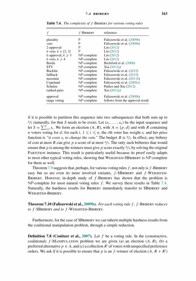
7 .4 bribery 163
Table 7.4. The complexity of f -Bribery for various voting rules
f f -Bribery reference
plurality P Faliszewski et al. (2009b)veto P Faliszewski et al. (2009b)2-approval P Lin (2012)k-veto, k ∈ {2, 3} P Lin (2012)k-approval, k � 3 NP-complete Lin (2012)k-veto, k � 4 NP-complete Lin (2012)Borda NP-complete Brelsford et al. (2008)STV NP-complete Xia (2012a)Bucklin NP-complete Faliszewski et al. (2015)fallback NP-complete Faliszewski et al. (2015)maximin NP-complete Faliszewski et al. (2011b)Copeland NP-complete Faliszewski et al. (2009c)Schulze NP-complete Parkes and Xia (2012)ranked pairs NP-complete Xia (2012a)
approval NP-complete Faliszewski et al. (2009b)range voting NP-complete follows from the approval result
if it is possible to partition this sequence into two subsequences that both sum up toS/2 (naturally, for that S needs to be even). Let (s1, . . . , sn) be the input sequence andlet S = ∑n
i=1 si . We form an election (A, R), with A = {p, d} and with R containingn voters voting for d; for each i, 1 � i � n, the ith voter has weight si and her pricefunction is “it costs si to change the vote.” The budget B is S/2. In effect, any briberyof cost at most B can give p a score of at most S/2. The only such briberies that wouldensure that p is among the winners must give p score exactly S/2, by solving the originalPartition instance. This result is particularly useful because its proof easily adaptsto most other typical voting rules, showing that Weighted-$Bribery is NP-completefor them as well.
Theorem 7.9 suggests that, perhaps, for various voting rules f , not only is f -Briberyeasy but so are even its more involved variants, f -$Bribery and f -Weighted-Bribery. However, in-depth study of f -Bribery has shown that the problem isNP-complete for most natural voting rules f . We survey these results in Table 7.4.Naturally, the hardness results for Bribery immediately transfer to $Bribery andWeighted-Bribery.
Theorem 7.10 (Faliszewski et al., 2009b). For each voting rule f , f -Bribery reducesto f -$Bribery and to f -Weighted-Bribery.
Furthermore, for the case of $Bribery we can inherit multiple hardness results fromthe coalitional manipulation problem, through a simple reduction.
Definition 7.8 (Conitzer et al., 2007). Let f be a voting rule. In the (constructive,coalitional) f -Manipulation problem we are given (a) an election (A, R), (b) apreferred alternative p ∈ A, and (c) a collection R′ of voters with unspecified preferenceorders. We ask if it is possible to ensure that p is an f -winner of election (A, R + R′)
164 7 control and bribery in voting
by setting the preference orders of the voters in R′. The (constructive, coalitional) f -Weighted-Manipulation problem is defined analogously, but for weighted elections,where the manipulators’ weights are given.
Theorem 7.11 (Faliszewski et al., 2009b). For each voting rule f , f -Manipula-tion reduces to f -$Bribery, and f -Weighted-Manipulation reduces to f -Weighted-$Bribery.
For the case of Swap-Bribery, hardness results are even more abundant. Elkindet al. (2009c) have shown that the problem is NP-complete for k-approval (for k � 2)8
and for Borda, Copeland, and maximin (for the latter three systems, NP-hardness holdseven for Shift-Bribery, a special case of Swap-Bribery where the swaps have toinvolve the preferred candidate). Furthermore, the Swap-Bribery problem generalizesthe Possible-Winner problem, which itself generalizes the Manipulation problem.
Definition 7.9 (Konczak and Lang, 2005). Let f be a voting rule. In the f -Possible-Winner problem we are given (a) an election (A, R), where the voters in R arerepresented through (possibly) partial orders, and (b) an alternative p ∈ A. We ask ifit is possible to extend the partial orders in R to linear orders in such a way that p is anf -winner of the resulting election.
Theorem 7.12 (Elkind et al., 2009c). For each voting rule f , f -Possible-Winnerreduces to f -Swap-Bribery.
Xia and Conitzer (2011a) have shown hardness of Possible-Winner for a numberof voting rules (including STV, ranked pairs, Borda, Copeland, maximin, and manyother rules); Betzler and Dorn (2010) together with Baumeister and Rothe (2012) showa dichotomy result regarding the complexity of Possible-Winner for pure scoringrules, obtaining hardness for almost all of them (see Chapter 10 and Section 4.3.2 inthe book chapter by Baumeister and Rothe (2015) for more details on the Possible-Winner problem and on related issues). By Theorem 7.12, these hardness resultsimmediately translate to hardness results for Swap-Bribery and the same voting rules.
Such an overwhelming number of hardness results (either shown directly or impliedby Theorems 7.11 and 7.12) suggests that, perhaps, Swap-Bribery is too generala problem. That is why Elkind et al. (2009c) defined Shift-Bribery, a variant ofSwap-Bribery where, as mentioned earlier, the only legal briberies shift the preferredcandidate up in the voters’ preference orders. While this problem turned out to typi-cally be NP-complete as well, Elkind et al. (2009c), Elkind and Faliszewski (2010), andSchlotter et al. (2011) have found some interesting polynomial-time algorithms, exactand approximate, and Bredereck et al. (2014b) have studied the parameterized com-plexity of Shift-Bribery (see Section 7.5 for more motivating discussions regardingShift-Bribery).
We now show that (the optimization variant of) Borda-Shift-Bribery can be effi-ciently approximated within a factor of 2.
Theorem 7.13 (Elkind et al., 2009c). There is a polynomial-time 2-approximationalgorithm for the cost of a cheapest shift bribery under Borda voting.
8 The result for k = 2 follows from the work of Betzler and Dorn (2010); for k = 1 the problem is in P; fork = m/2, where m is the number of alternatives, Elkind et al. (2009c) have shown hardness even for the case ofa single voter.

7 .4 bribery 165
Proof sketch. Consider an instance of our problem where the goal is to ensure candidatep’s victory. By definition, the only possible actions are shifting p forward in (some of)the votes (costs are specified through swap-bribery price functions where swaps thatdo not involve p have infinite cost and we can think of shifting p forward in terms ofits swaps with other candidates).
We start with two observations. First, there is a polynomial-time algorithm thatgiven an instance of the optimization variant of Borda-Shift-Bribery computes thecost of a cheapest shift bribery that gives p a given number of points (the algorithmuses standard dynamic programming). Second, if there is a successful shift bribery thatincreases the score of p by K points, then every shift bribery that increases p’s scoreby 2K points is successful (the best imaginable shift bribery gets K points for p insuch a way that in each swap it increases the score of p and decreases the score ofits strongest competitor; we achieve the same—or better—effect by getting 2K pointsfor p).
Now the algorithm proceeds as follows: First, we guess the number K of pointsthat p gets in the optimal solution. Then, we guess a number K ′, K ′ � K . (Becausewe are dealing with Borda elections, both guesses boil down to trying polynomiallymany computation paths.) We compute a cheapest shift bribery S1 that gives K pointsto p. Then, we compute a cheapest shift bribery S2 that gives K ′ additional points top (we apply S2 after we have applied S1). We claim that S1 + S2 (that is, the two shiftbriberies taken together) form a 2-approximate solution.
Why is this so? Consider some optimal shift bribery O that ensures that p wins.By assumption, this shift bribery obtains K points for p. Now imagine the followingsituation: We start with the original election and perform only those swaps that areincluded in both O and S1. In effect, p gains some K ′′ points. If we continued withthe optimal solution, p would obtain additional K − K ′′ points and would become awinner of the election. By our second observation, this means that if after performingthe swaps that occur both in O and in S1 we obtain additional 2(K − K ′′) points forp, p certainly wins. We obtain the first of these K − K ′′ points by simply performingthe remaining swaps from S1. For the second K − K ′′ points, we can assume that weguessed K ′ = K − K ′′. In effect, performing the swaps from S2 ensures p’s victory.Furthermore, by definition of S1 we know that its cost is no higher than that of O. Onthe other hand, the cost of S2 also has to be at most as high as that of O because, bydefinition, the cost of S2 cannot be higher than the cost of the shift bribery that containsexactly the swaps that are in O but not in S1.
So far, there has been relatively little research on how to cope with the hardness ofbribery problems (except for results regarding special cases such as Shift-Bribery, asseen in the preceding theorem). For example, many parameterized-complexity resultsboil down to polynomial-time algorithms for the case where the number of candi-dates is constant. In this case, bribery problems can either be solved by an appro-priate brute-force search, or by solving a linear integer program using the algorithmof Lenstra, Jr. (1983); see the papers of Faliszewski et al. (2009b, 2011b), Elkindet al. (2009c), Dorn and Schlotter (2012), and Hemaspaandra et al. (2013b) for exam-ples. These approaches, however, do not work for weighted elections and, indeed, forweighted elections bribery problems are typically NP-hard (see, e.g., the dichotomyresults of Faliszewski et al. (2009b)). On the other hand, there are several detailed
166 7 control and bribery in voting
studies of parameterized complexity of Swap-Bribery (due to Dorn and Schlotter,2012), Support-Bribery (Schlotter et al. (2011); we omit the discussion of Support-Bribery), and Shift-Bribery (Bredereck et al., 2014b).
Another natural way of coping with the hardness of bribery problems would be todesign approximation algorithms. Brelsford et al. (2008) have made some attemptsin this direction (though, using a rather involved goal function instead of approxi-mating the cost of a successful bribery), Faliszewski (2008) gave a fully polynomial-time approximation scheme for plurality-Weighted-$Bribery, and Xia (2012a) gaveseveral approximation algorithms for destructive bribery problems (where the goalis to ensure, through buying votes, that some candidate does not win the election).There are also approximation results regarding Shift-Bribery (due to Elkind andFaliszewski, 2010; Bredereck et al., 2014b). While surprising at first, this limitedenthusiasm for studying approximation algorithms for bribery problems can, to someextent, be understood. Theorems 7.11 and 7.12 show how to reduce the Manipulationand Possible-Winner problems to appropriate $Bribery and Swap-Bribery prob-lems, and they do so via showing that a given Manipulation (Possible-Winner)instance is a “yes” instance if and only if there is a zero-cost bribery. This meansthat, unless P = NP, those $Bribery and Swap-Bribery problems whose hardnesscan be shown via Theorems 7.11 and 7.12 do not have constant-factor polynomial-time approximation algorithms (for finding the cheapest successful bribery). Nonethe-less, it is interesting to study the approximability of f -Bribery for various votingrules f .
It would also be interesting to study the complexity of bribery in elections withrestricted domains, for example, in single-peaked elections. While this direction hasbeen pursued successfully for the case of control, we are aware of only a single paperthat attempted it for bribery (Brandt et al., 2010a), showing that, indeed, for single-peaked elections bribery problems often become easy (see also Section 5.4 in the bookchapter by Hemaspaandra et al. (2015)).
7.4.2 Other Bribery Problems
So far, we have focused on the most standard election model, where voter preferencesare represented by total orders over the set of alternatives. Naturally, there are numerousother settings in which bribery was studied, and in what follows we give several (thoughcertainly not all) examples of such settings.
Mattei et al. (2012a) have considered bribery in combinatorial domains, wherethe voters express their preferences over bundles of alternatives in a certain compactway. This compact representation can lead to quite interesting results. The particularlanguage used to express preferences in the work of Mattei et al. (2012a) (CP-nets)does not allow one to express certain preference orders and, as a result, Bribery fork-approval becomes easy in this model (see Chapter 9 for more details on voting incombinatorial domains). If there are no direct interrelations between the bundles ofitems, it may be more reasonable to model bribery as the lobbying problem (studied byChristian et al. (2007) and later on by Bredereck et al. (2014a) and Binkele-Raible et al.(2014)): We are given a collection of yes/no votes over all items independently, wherean item is accepted with a simple majority of yes votes, and is rejected otherwise. The

7 .5 a positive look 167
lobby’s goal is to change the outcome to its liking by bribing certain voters withoutexceeding its budget.
Examples of bribery problems in other settings include, for example, the work ofBaumeister et al. (2011) on bribery in judgment aggregation (see Chapter 17 and thebook chapter by Baumeister et al. (2015) for more details on judgment aggregation), thework of Rey and Rothe (2011) and Marple et al. (2014) on bribery in path-disruptiongames, and the work of Mattei et al. (2012b) on bribery in tournaments.
7.5 A Positive Look
There are a number of settings where control and bribery (and similar problems) havepositive interpretations (from particular points of view). In the following we very brieflylist a few examples of such settings.
Election control problems deal with affecting their structure in order to change thewinner. Instead of viewing this as someone manipulating the result, we can think of itas predicting the winners given how the election’s structure may change. For example,this research direction was pursued by Chevaleyre et al. (2012) and Baumeister et al.(2012c). Specifically, Chevaleyre et al. (2012) have studied a situation where we havealready elicited voters’ preferences regarding some set of candidates, but afterwardsome new candidates appeared, of whom we have no knowledge whatsoever. Naturally,possibly each new candidate can be better than each old one, so each of them, possibly,might win the election. However, can we decide which of the original candidates stillhave chances of winning? This problem of predicting possible winners is very close inspirit to control by adding candidates (and to cloning; see later), though—formally—itis a special case of the Possible-Winner problem (and, as such, it is a special case ofthe Swap-Bribery problem).
Another way of predicting election winners was suggested by Wojtas and Fal-iszewski (2012), who have used counting variants of election control problems. Inparticular, they considered the following setting: We know the preference orders of thevoters, but we do not know which of them will eventually cast votes. Having some priordistribution on the number of voters that do cast votes (and assuming that if k votersparticipate in the election, then each size-k subset of voters is equally likely to vote),what is the probability that a given candidate wins? Formally, this problem reduces tocounting the number of ways of adding (deleting) voters to (from) an election to ensurea given candidate’s victory.
Quite interestingly, many of the problems that model attacks on elections havedirect applications in protecting them. For example, in the margin-of-victory problem(see, e.g., the work of Cary (2011), Magrino et al. (2011), Xia (2012a), and Reischet al. (2014)) we ask how many voters need to cast different votes to change theresult of an election. If this number is high then it is unlikely that the election wastampered with. However, if this number is low, it means that it would have been easy tomanipulate the result in some way and thus we should carefully check the election. Themargin-of-victory problem is, in some sense, simply a destructive bribery problem.Similarly, Birrell and Pass (2011) have used bribery-related problems in the context ofapproximate strategyproofness of voting rules. Yet another application of a control-like
168 7 control and bribery in voting
problem to protect elections was given by Elkind et al. (2012a). They have consideredthe problem of candidate cloning, where some candidate c is replaced by a number ofclones, c1, . . . , ct , that—from the point of view of the voters—are indistinguishable(consider, for example, a party submitting several candidates for a given position andthe voters forming their preference orders based on party membership only). If anelection is single-peaked and we clone a candidate, it is likely that this election ceasesto be single-peaked. Motivated by this observation, Elkind et al. (2012a) have givenan algorithm that finds an optimal “decloning” of the candidates, so that the resultingelection is single-peaked (similar results, though in a different context, were latergiven by Cornaz et al. (2012, 2013); we also mention that cloning, originally definedby Tideman (1987) and by Zavist and Tideman (1989), resembles control by addingcandidates; its computational analysis is due to Elkind et al. (2011a)).
Finally, let us mention some positive interpretations of bribery problems. In politicalelections, prior to casting the votes, the candidates run their campaigns and wish toconvince the voters to rank them as highly as possible. Naturally, running a campaignhas cost (both in terms of money and in terms of invested time) and it is important for thecandidates to decide which voters they should try to convince. However, deciding howmuch effort to spend on each voter (or, group of voters) is just the bribery problem (seethe work of Hazon et al. (2013) for a different twist on this idea). With the campaignmanagement interpretation in mind, it is natural to study various special cases of thebribery problems. Indeed, Shift-Bribery of Elkind et al. (2009c), where we can onlyconvince the voters to rank the preferred candidate higher and we cannot affect therelative order of the other candidates, models campaign management in a natural way.While the Shift-Bribery problem is NP-hard for many voting rules, Elkind et al.(2009c) have given a 2-approximation algorithm for this problem with Borda’s rule(see Theorem 7.13 here), Elkind and Faliszewski (2010) have extended this result to allscoring rules (and provided weaker approximations for Copeland and maximin), andSchlotter et al. (2011) have shown that Shift-Bribery is in P for Bucklin and fallbackvoting. These results for Bucklin and fallback voting were recently complementedby Faliszewski et al. (2015) who studied various bribery problems for these rules,including so-called Extension-Bribery, introduced by Baumeister et al. (2012a) inthe context of campaign management in the presence of truncated ballots.
7.6 Summary
We surveyed the known results on control and bribery. While often studied in thecontext of attacking elections, these problems also have many other applications andinterpretations, often very positive ones. Many NP-hardness results have been obtained,yet recent work focuses on solving these problems effectively, either by approximationor fixed-parameter tractable algorithms, or efficient heuristics. We strongly encouragethe readers to study control and bribery and to add their own contributions to the field.
CHAPTER 8
Rationalizations of Voting Rules
Edith Elkind and Arkadii Slinko
8.1 Introduction
From antiquity to these days, voting has been an important tool for making collectivedecisions that accommodate the preferences of all participants. Historically, a remark-ably diverse set of voting rules have been used (see, e.g., Brams and Fishburn, 2002),with several new voting rules proposed in the last three decades (Tideman, 1987;Schulze, 2003; Balinski and Laraki, 2010). Thus, when decision-makers need to selecta voting rule, they have plenty of choice: should they aggregate their opinions usingsomething as basic as Plurality voting or something as sophisticated as Ranked Pairs?Or should they perhaps design a new voting rule to capture the specific features of theirsetting?
Perhaps the best known way to answer this question is to use the axiomatic approach,that is, identify desirable properties of a voting rule and then choose (or construct) a rulethat has all of these properties. This line of work was initiated by Arrow (1951) and led toa great number of impossibility theorems, as it turned out that some desirable propertiesof voting systems are incompatible. By relaxing these properties, researchers obtainedaxiomatic characterizations of a number of classical voting rules, such as Majority(May, 1952), Borda (Young, 1975), and Kemeny (Young and Levenglick, 1978); seethe survey by Chebotarev and Shamis (1998) as well as Chapter 2.
However, early applications of voting suggest a different perspective on this question.It is fair to say that in the Middle Ages voting was most often used by religiousorganizations (Uckelman and Uckelman, 2010). The predominant view in ecclesiasticalelections was that God’s cause needed the most consecrated talent that could be foundfor leadership in the church. Moreover, it was believed that God knew who the bestcandidate was, so the purpose of elections was to reveal God’s will. It is therefore notsurprising that when the Marquis de Condorcet (1785) undertook the first attempt atsystematization of voting rules, he was influenced by the philosophy of church elections.His view was that the aim of voting is to determine the “best” decision for the societywhen voters are prone to making mistakes. This approach assumes that there is anobjectively correct choice, but voters have different opinions due to errors of judgment;
169
170 8 rationalizations of voting rules
absent these errors, they would all agree on the most suitable alternative. Thus, oneshould aim to design a voting rule that maximizes the probability of identifying thebest choice. Depending on the model of “noise” or “mistakes” in voters’ judgment, weget different voting rules. In statistics, this approach is known as maximum likelihoodestimation (MLE): it tries to estimate the state of the world (which is hidden) that ismost likely to produce the observed noisy data.
A somewhat different, but related approach, which takes its roots in ideas of CharlesDodgson (1876), can be called consensus-based. The society agrees on a notion ofa consensus (for example, we could say that there is a consensus if all voters agreewhich alternative is the best, or if there exists a Condorcet winner), and the result ofeach election is viewed as an imperfect approximation to a consensus. Specifically, if apreference profile R is a consensus, then we pick the consensus winner, and otherwisewe output the winners of consensus profiles R′ that are as close to R as possible.Alternatively, we may say that the society looks for a minimal change to the givenpreference profile that turns it into a profile with an indisputable winner. At the heartof this approach is the agreement as to (1) which preference profiles should be viewedas consensual and (2) what is the appropriate notion of closeness among preferenceprofiles. It turns out that many common voting rules can be explained and classified bydifferent choices of these parameters.
In this chapter we will survey the MLE framework and the consensus-based frame-work, starting with the latter. We demonstrate that both frameworks can be used torationalize many common voting rules, with the consensus-based framework beingsomewhat more versatile. We also establish some connections between the two frame-works. We remark that these two frameworks are not the only alternatives to theaxiomatic analysis. For instance, Camps et al. (2014) put forward an approach thatis based on propositional logic. Furthermore, in economic literature the term “ratio-nalization” usually refers to explaining the behavior of an agent or a group of agentsvia an acyclic (or transitive) preference relation, and there is a large body of literaturethat investigates which voting rules are rationalizable in this sense (see Bossert andSuzumura, 2010, for a survey). In this chapter, we focus on the MLE framework andthe consensus-based framework because these two methods for rationalizing votingrules are interesting from a computational perspective: as we will see, explaining avoting rule via a consensus and a “good” measure of closeness implies upper boundson its algorithmic complexity, whereas MLE-based voting rules are desirable for manyapplications, such as crowdsourcing, and therefore implementing them efficiently is ofparamount importance.
In what follows, we assume that the set of alternatives is A and |A| = m; we use theterms alternatives and candidates interchangeably. Also, unless specified otherwise,voters’ preferences and ballots are assumed to be linear orders over A.
8.2 Consensus-Based Rules
The goal of the consensus-based approach is to reach a compromise among all voters,that is, to arrive at a situation where there is agreement in society as to which outcomeis the best. This may require persuading some voters to modify their opinions in minor
8 .2 consensus-based rules 171
ways, and, as a result, to make small changes to their ballots. Obviously it is desirableto minimize the number and magnitude of these changes. Thus, the best alternativesare the ones for which the agreement can be reached at the smallest cost (measuredby the total amount of changes). In other words, given an arbitrary preference profile,we proceed by identifying the consensual profiles that are most similar to it andoutputting their winners. The result then depends on how we define consensual profilesand how we measure the magnitude of change in votes. The latter question is usuallyaddressed by using a distance over the space of profiles; this is why voting rules thatcan be obtained in this manner are called distance rationalizable. Often, this distance isobtained by computing the number of “unit changes” needed to transform one profileinto the other, where the notion of “unit change” may vary from one voting rule toanother.
This method of constructing voting rules can be traced back to Dodgson (1876), whowas the first to define a voting rule in this manner (for a specific notion of consensus anda specific distance between profiles, see Section 8.2.1). More recently, it was formalizedand studied by Nitzan (1981), Lerer and Nitzan (1985), Campbell and Nitzan (1986),and Baigent (1987), and subsequently by Meskanen and Nurmi (2008) and Elkindet al. (2010a, 2010b, 2011b, 2012b); we also point the reader to the survey of Eckertand Klamler (2011). It turns out that many classic voting rules can be obtained in thismanner; Meskanen and Nurmi (2008) put together an extensive catalogue of distancerationalizations of common voting rules, with additional examples provided by Elkindet al. (2010b, 2012b). Furthermore, many properties of voting rules can be derived fromtheir distance rationalizations: a voting rule can be shown to have “nice” properties ifit can be rationalized via a “nice” consensus class and a “nice” distance. This makesthe distance rationalizability approach eminently suitable for constructing new votingrules: it allows us to combine known distances and consensus classes, and deriveconclusions about the resulting rules based on the properties of their components.
We start by presenting a few examples that illustrate the concepts of consensus anddistance to consensus, followed by a formal definition and a discussion of propertiesof distance rationalizable voting rules.
8.2.1 Examples
The examples in this section are taken from the work of Meskanen and Nurmi (2008)and Elkind et al. (2012b); see these papers for additional references. We provide briefdescriptions of the voting rules we consider; for formal definitions the reader is referredto Chapter 2.
Dodgson. Perhaps the most canonical example of the consensus-based approach isthe Dodgson rule. Recall that winner determination under this rule proceeds asfollows. If the given preference profile has a Condorcet winner, that is, a candidatethat beats every other candidate in a pairwise election, then this candidate isdeclared the unique Dodgson winner. Otherwise, for every candidate c we computeher Dodgson score, that is, the number of swaps of adjacent candidates in voters’ballots that need to be performed in order to make c a Condorcet winner. We thenoutput all candidates with the smallest Dodgson score. This definition follows the
172 8 rationalizations of voting rules
principles of the distance rationalizability framework: the underlying notion ofagreement is the existence of a Condorcet winner, and the unit changes are swapsof adjacent candidates. This notion of unit change corresponds to a distance onrankings known as the swap distance, which is the number of swaps of adjacentcandidates needed to transform one ranking into the other. We refer the reader toChapter 5 for a complexity-theoretic analysis of the Dodgson rule.
Kemeny. The Kemeny rule is also defined in terms of the swap distance. While it ismore common to view this rule as a social preference function, that is, a mappingthat, given a preference profile, outputs a set of rankings, in this section we willbe interested in the interpretation of this rule as a social choice function. Underthe Kemeny rule, we identify all rankings that minimize the total swap distanceto the voters’ ballots. The associated social preference function then outputs allsuch rankings, whereas the Kemeny social choice function (which we will referto as the Kemeny rule) outputs all candidates that are ranked first in at least oneof these rankings. This rule can be viewed as another example of the distancerationalizability approach: the consensual profiles are ones where all votes areidentical, and the unit changes are the same as for the Dodgson rule, that is, swapsof adjacent candidates.
Plurality. Under Plurality rule, each candidate gets one point from each voter whoranks her first; the winners are the candidates with the largest number of points.Because Plurality considers voters’ top candidates only, it is natural to use anotion of consensus that also has this property: we say that there is an agreementin the society if all voters rank the same candidate first. Now, consider an n-voterpreference profile. If some candidate a receives na ≤ n Plurality votes, there aren − na voters who do not rank her first. Thus, if we want to turn this profile into aconsensus where everyone ranks a first, and we are allowed to change the ballotsin any way we like (at a unit cost per ballot), we have to modify n − na ballots. Inother words, if our notion of a unit change is an arbitrary modification of an entireballot, then the number of unit changes required to make a candidate a consensuswinner is inversely related to her Plurality score. In particular, the candidates forwhom the number of required unit changes is minimal are the Plurality winners.Alternatively, we can define a unit change as a swap of two (not necessarilyadjacent) candidates; the preceding argument still applies, thereby showing thatthis construction also leads to the Plurality rule.
Borda. Recall that the Borda score of a candidate a in an n-voter, m-candidate pro-file is given by (m − r1) + · · · + (m − rn) = nm −∑
i ri , where ri , i = 1, . . . , n,is the rank of a in the ith ballot. To distance rationalize this rule, we use the samenotion of consensus as for the Plurality rule (i.e., all voters agree on who is thebest candidate) and the same notion of unit change as for the Dodgson rule andthe Kemeny rule, namely, a swap of adjacent candidates. Indeed, to ensure thata is ranked first by voter i, we need to perform ri − 1 swaps of adjacent candi-dates. Consequently, making a the unanimous winner requires
∑i ri − n swaps.
That is, the number of swaps required to make a candidate a consensus winneris inversely related to her Borda score. This construction, which dates back toFarkas and Nitzan (1979), can be extended to scoring rules other than Borda, byassigning appropriate weights to the swaps (Lerer and Nitzan, 1985).

8 .2 consensus-based rules 173
Copeland. The Copeland score of a candidate a can be defined as the number ofpairwise elections that a wins (a may also get additional points for the pairwiseelections that end in a tie; in what follows we focus on elections with an oddnumber of voters to avoid dealing with ties). The Copeland winners are thecandidates with the highest Copeland score. For this rule, an appropriate notionof consensus is the existence of a Condorcet winner. As for the notion of unitchange, it is convenient to formulate it in terms of the pairwise majority graph.Recall that the pairwise majority graph G(R) of a profile R over a candidate setA is the directed graph whose vertex set is A and there is a directed edge fromcandidate a to candidate b if a strict majority of voters in R prefer a to b. Considertwo n-voter profiles R1 and R2 over a candidate set A; assume that n is odd. Anatural notion of a unit change in this setting is an edge reversal, that is, a pair(a, b) ∈ A × A such that in G(R1) there is an edge from a to b, whereas in G(R2)there is an edge from b to a. The distance between R1 and R2 is then defined as thenumber of edge reversals. To see that this distance combined with the Condorcetconsensus rationalizes the Copeland rule, note that if a candidate’s Copeland scoreis s, she can be made the Condorcet winner by reversing m − 1 − s edges, sothe number of edge reversals and the candidate’s Copeland score are inverselyrelated.
Maximin. The Maximin score of a candidate a in an n-voter profile R over acandidate set A is the number of votes that a gets in her most difficult pairwiseelection (i.e., minb∈A nab, where nab is the number of voters in R who prefera to b); the winners are the candidates with the highest score. Suppose thatR has no Condorcet winner, and consider a candidate a ∈ A. Let b be a’s mostdifficult opponent, that is, a’s Maximin score is sa = nab; note that sa ≤ n
2 < n+12 ,
because a is not a Condorcet winner. Then if we add n + 1 − 2sa ballots where a
is ranked first, a will be the Condorcet winner in the resulting profile (which has2n + 1 − 2sa voters, with n + 1 − sa of these voters ranking a above c for everyc ∈ A). On the other hand, if we add k < n + 1 − 2sa ballots, we obtain a profilewhere at least n − sa voters out of n + k prefer b to a; as 2(n − sa) ≥ n + k, thismeans that at least half of the voters in this profile prefer b to a, so a is not aCondorcet winner. Thus, a candidate’s Maximin score is inversely related to thenumber of ballots that need to be added in order to obtain a profile where thiscandidate is the Condorcet winner.
This argument explains the Maximin rule in the language of agreement andchanges. However, this explanation does not quite fit our framework, becauseit uses a notion of unit change (adding a single ballot) that does not directlycorrespond to a distance. The problem here is that a distance is supposed to besymmetric (see Section 8.2.2), whereas adding ballots is an inherently asym-metric operation: if we can turn R into R′ by adding s ballots, we cannot turnR′ into R by adding s ballots. It turns out, however, that the Maximin rulecan be rationalized via the distance that measures the number of ballots thatneed to be added or deleted to turn one profile into another (see Elkind et al.,2012b, for details). Intuitively, this is because for the purpose of reaching aCondorcet consensus adding a ballot is always at least as useful as deleting aballot.
174 8 rationalizations of voting rules
We remark that there is another voting rule that is defined in terms of deletingballots so as to obtain a Condorcet consensus, namely, the Young rule, which isdiscussed in Chapter 5. While the Young rule, too, can be distance-rationalized,the construction is quite a bit more complicated than for Maximin (Elkind et al.,2012b).
These examples raise a number of questions. First, is it the case that all votingrules can be explained within the consensus-based framework? Second, what are theappropriate notions of consensus and distance to consensus? Third, can we derive anyconclusions about a voting rule based on the notion of consensus and distance thatexplain it? To answer these questions, we need to define our framework formally.
8.2.2 Formal Model
The consensus-based framework that has been introduced informally so far has twoessential components: the definition of what it means to have an agreement in thesociety and the notion of distance between preference profiles. We will now discussboth of these components in detail. Our presentation mostly follows Elkind et al.(2010b).
Consensus Classes
Informally, we say that a preference profile R is a consensus if it has an undisputedwinner reflecting a certain concept of agreement in the society. Formally, a consensusclass for a set of candidates A is a pair K = (X , w) where X is a nonempty set ofprofiles over A and w : X → A is a mapping that assigns a unique candidate to eachprofile in X ; this candidate is called the consensus choice (winner).1 We require K tobe anonymous and neutral, in the following sense: For every profile R ∈ X a profileR′ obtained from R by permuting voters satisfies R′ ∈ X and w(R′) = w(R), andthe profile R′′ obtained from R by renaming candidates according to a permutationπ : A → A satisfies R′′ ∈ X and w(R′′) = π(w(R)) (i.e., the winner under R′′ isobtained by renaming the winner under R according to π).
The following classes of preference profiles have been historically viewed as situa-tions of consensus:
Strong unanimity. This class, denotedS , consists of profiles where all voters reportthe same preference order. The consensus choice is the candidate ranked first byall voters. The reader may note that we have used this notion of consensus inSection 8.2.1 to rationalize the Kemeny rule. Interestingly, it can also be used toprovide an alternative rationalization of the Plurality rule (Elkind et al., 2010a).
Unanimity. This class, denoted U , consists of profiles where all voters rank somecandidate c first (but may disagree on the ranking of the remaining candidates).The consensus choice is this candidate c. This consensus class appears in our
1 One can also consider situations in which the voters reach a consensus that several candidates are equally wellqualified to be elected; this may happen, for example, under Approval voting when all voters approve the sameset of candidates. However, in what follows we limit ourselves to consensus classes with unique winners.

8 .2 consensus-based rules 175
rationalizations of Plurality and Borda. It is also used to rationalize other scoringrules (Lerer and Nitzan, 1985; Elkind et al., 2009a).
Majority. This class, denoted M, consists of profiles where more than half of thevoters rank some candidate c first. The consensus choice is this candidate c. Thisnotion of consensus can be used to rationalize Plurality and a simplified versionof the Bucklin rule (Elkind et al., 2010b).
Condorcet. This class, denoted C, consists of profiles with a Condorcet winner.The consensus choice is the Condorcet winner. This notion of consensus appearsin our rationalizations of the Dodgson rule, the Copeland rule, and Maximin.
Transitivity. This class, denoted T , consists of profiles whose majority relationis transitive, that is, for every triple of candidates a, b, c ∈ A it holds that if amajority of voters prefer a to b and a majority of voters prefer b to c, then amajority of voters prefer a to c. Such profiles always have a Condorcet winner, sowe define the consensus choice to be the Condorcet winner. This consensus classcan be used to rationalize the Slater rule (Meskanen and Nurmi, 2008).
It is easy to see that we have the following containment relations among the consen-sus classes: S ⊂ U ⊂ M ⊂ C and S ⊂ T ⊂ C. However, U and T are incomparable,that is, U �⊆ T and T �⊆ U . Similarly, we have M �⊆ T and T �⊆ M.
Remark 8.1. A consensus class (X , w) can be viewed as a voting rule with domainX that always outputs a unique candidate. Conversely, every anonymous and neutralvoting rule f such that |f (R)| = 1 for at least one profile R defines a consensus class:if f is defined on the set of all profiles over a candidate set A, we can define a consensusclass Kf = (Xf , wf ) by setting Xf = {R | |f (R)| = 1} and for each R ∈ Xf definingwf (R) to be the unique candidate in f (R). That is, this consensus class consists of allprofiles on which f makes a definitive choice. The condition that |f (R)| = 1 for someprofile R is necessary to ensure that Xf �= ∅.
There are other consensus classes one could consider: for example, one could studya 2/3-variant of the majority consensus M, where more than 2/3 of the voters rank thesame candidate first (this choice of threshold stems from the observation that in manycountries changes to the constitution require the support of two thirds of the eligiblevoters). However, these five classes appear to be representative enough to rationalizemany interesting voting rules.
Distances
To capture the idea of measuring the magnitude of changes in a preference profile, weuse distances on profiles. Recall that a distance on a set X is a mapping d : X × X →R ∪ {+∞} such that for every x, y, z ∈ X the following four conditions are satisfied:
(a) d(x, y) � 0 (nonnegativity);(b) d(x, y) = 0 if and only if x = y (identity of indiscernibles);(c) d(x, y) = d(y, x) (symmetry);(d) d(x, y) � d(x, z) + d(z, y) (triangle inequality).
A mapping that satisfies (a), (c), and (d), but not (b), is called a pseudodistance.
176 8 rationalizations of voting rules
For distance rationalizability constructions, we need distances that are defined onpairs of profiles. Usually, it is enough to only consider pairs of profiles with the sameset of candidates (this will be the case for all distances considered in this chapter), andin many cases it suffices to only consider pairs of profiles with the same number ofvoters. In particular, to construct a distance on the space of all n-voter profiles over afixed set of candidates A, we can take a suitable distance d on the space L(A) of alllinear orders over A and extend it to a distance d over the space of all n-voter preferenceprofiles Ln(A) by setting
d ((u1, . . . , un), (v1, . . . , vn)) = d(u1, v1) + . . . + d(un, vn). (8.1)
It can be shown that d satisfies all distance axioms whenever d does. This method ofbuilding distances over profiles from distances over votes will play an important rolein our analysis (see Section 8.2.4).
We will now present several examples of distances on the space of preferenceprofiles. Some of these distances should look familiar to the reader, as they were usedto rationalize voting rules in Section 8.2.1.
Discrete distance. The discrete distance is defined on pairs of profiles with thesame set of candidates A and the same number of voters n using formula (8.1);the underlying distance on L(A) is given by
ddiscr(u, v) ={
0 if u = v,
1 if u �= v.
This distance was used in our rationalization of the Plurality rule.Swap distance. The swap distance, which is also known as the Kendall tau dis-
tance, the Kemeny distance, the Dodgson distance, and the bubble-sort distance(Kendall and Gibbons, 1990), is also defined using formula (8.1). The underlyingdistance on L(A) is the swap distance between individual votes: dswap(u, v) isthe number of pairs (c, c′) ∈ A × A such that u ranks c above c′, but v ranks c′
above c.(Weighted) footrule distance. This distance is also known as Spearman distance,
or Spearman footrule (Kendall and Gibbons, 1990). Let pos(u, c) denote theposition of candidate c in vote u (the top candidate in u has position 1, and thebottom candidate in u has position m). Then the footrule distance on L(A) isgiven by
dfr(u, v) =∑c∈A
|pos(u, c) − pos(v, c)|.
That is, we measure the displacement of each candidate as we move from u tov, and then we take the sum over all candidates. This distance is extended topreference profiles using formula (8.1). The reader can verify that we can usethe footrule distance dfr instead of the swap distance in our rationalization of theBorda rule.
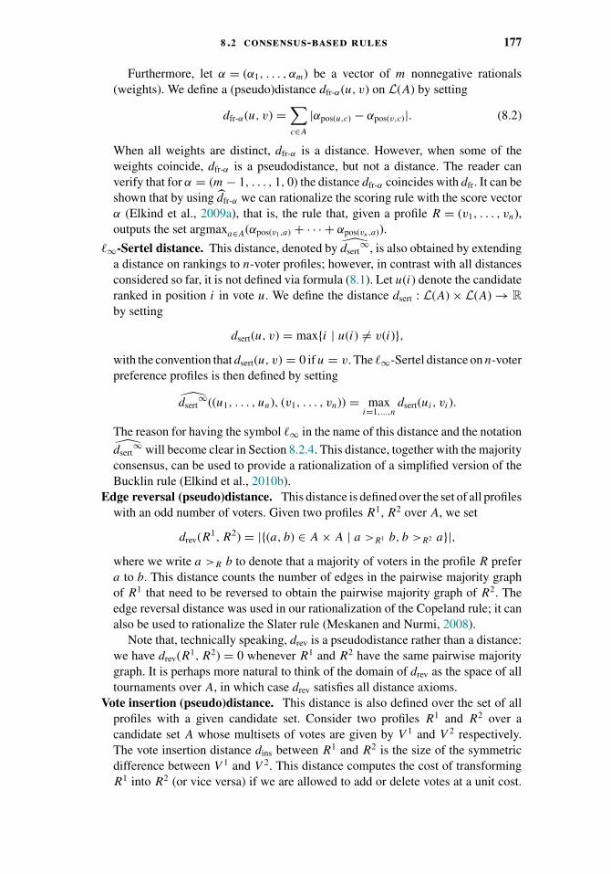
8 .2 consensus-based rules 177
Furthermore, let α = (α1, . . . , αm) be a vector of m nonnegative rationals(weights). We define a (pseudo)distance dfr-α(u, v) on L(A) by setting
dfr-α(u, v) =∑c∈A
|αpos(u,c) − αpos(v,c)|. (8.2)
When all weights are distinct, dfr-α is a distance. However, when some of theweights coincide, dfr-α is a pseudodistance, but not a distance. The reader canverify that for α = (m − 1, . . . , 1, 0) the distance dfr-α coincides with dfr. It can beshown that by using dfr-α we can rationalize the scoring rule with the score vectorα (Elkind et al., 2009a), that is, the rule that, given a profile R = (v1, . . . , vn),outputs the set argmaxa∈A(αpos(v1,a) + · · · + αpos(vn,a)).
∞-Sertel distance. This distance, denoted by dsert∞, is also obtained by extending
a distance on rankings to n-voter profiles; however, in contrast with all distancesconsidered so far, it is not defined via formula (8.1). Let u(i) denote the candidateranked in position i in vote u. We define the distance dsert : L(A) × L(A) → Rby setting
dsert(u, v) = max{i | u(i) �= v(i)},with the convention that dsert(u, v) = 0 if u = v. The ∞-Sertel distance on n-voterpreference profiles is then defined by setting
dsert∞((u1, . . . , un), (v1, . . . , vn)) = max
i=1,...,ndsert(ui, vi).
The reason for having the symbol ∞ in the name of this distance and the notation
dsert∞ will become clear in Section 8.2.4. This distance, together with the majority
consensus, can be used to provide a rationalization of a simplified version of theBucklin rule (Elkind et al., 2010b).
Edge reversal (pseudo)distance. This distance is defined over the set of all profileswith an odd number of voters. Given two profiles R1, R2 over A, we set
drev(R1, R2) = |{(a, b) ∈ A × A | a >R1 b, b >R2 a}|,where we write a >R b to denote that a majority of voters in the profile R prefera to b. This distance counts the number of edges in the pairwise majority graphof R1 that need to be reversed to obtain the pairwise majority graph of R2. Theedge reversal distance was used in our rationalization of the Copeland rule; it canalso be used to rationalize the Slater rule (Meskanen and Nurmi, 2008).
Note that, technically speaking, drev is a pseudodistance rather than a distance:we have drev(R1, R2) = 0 whenever R1 and R2 have the same pairwise majoritygraph. It is perhaps more natural to think of the domain of drev as the space of alltournaments over A, in which case drev satisfies all distance axioms.
Vote insertion (pseudo)distance. This distance is also defined over the set of allprofiles with a given candidate set. Consider two profiles R1 and R2 over acandidate set A whose multisets of votes are given by V 1 and V 2 respectively.The vote insertion distance dins between R1 and R2 is the size of the symmetricdifference between V 1 and V 2. This distance computes the cost of transformingR1 into R2 (or vice versa) if we are allowed to add or delete votes at a unit cost.
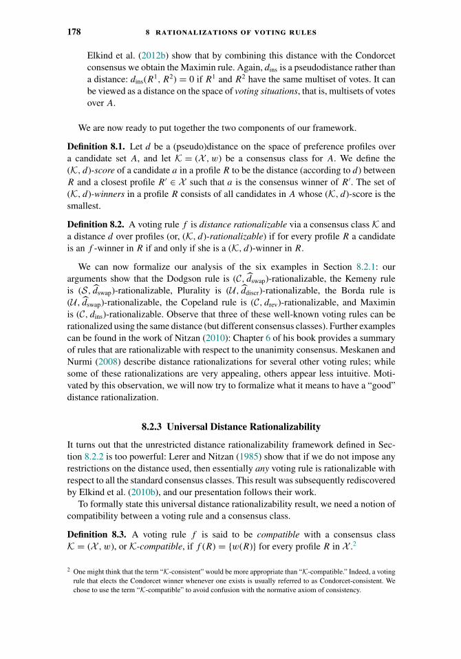
178 8 rationalizations of voting rules
Elkind et al. (2012b) show that by combining this distance with the Condorcetconsensus we obtain the Maximin rule. Again, dins is a pseudodistance rather thana distance: dins(R1, R2) = 0 if R1 and R2 have the same multiset of votes. It canbe viewed as a distance on the space of voting situations, that is, multisets of votesover A.
We are now ready to put together the two components of our framework.
Definition 8.1. Let d be a (pseudo)distance on the space of preference profiles overa candidate set A, and let K = (X , w) be a consensus class for A. We define the(K, d)-score of a candidate a in a profile R to be the distance (according to d) betweenR and a closest profile R′ ∈ X such that a is the consensus winner of R′. The set of(K, d)-winners in a profile R consists of all candidates in A whose (K, d)-score is thesmallest.
Definition 8.2. A voting rule f is distance rationalizable via a consensus class K anda distance d over profiles (or, (K, d)-rationalizable) if for every profile R a candidateis an f -winner in R if and only if she is a (K, d)-winner in R.
We can now formalize our analysis of the six examples in Section 8.2.1: ourarguments show that the Dodgson rule is (C, dswap)-rationalizable, the Kemeny ruleis (S, dswap)-rationalizable, Plurality is (U , ddiscr)-rationalizable, the Borda rule is(U , dswap)-rationalizable, the Copeland rule is (C, drev)-rationalizable, and Maximinis (C, dins)-rationalizable. Observe that three of these well-known voting rules can berationalized using the same distance (but different consensus classes). Further examplescan be found in the work of Nitzan (2010): Chapter 6 of his book provides a summaryof rules that are rationalizable with respect to the unanimity consensus. Meskanen andNurmi (2008) describe distance rationalizations for several other voting rules; whilesome of these rationalizations are very appealing, others appear less intuitive. Moti-vated by this observation, we will now try to formalize what it means to have a “good”distance rationalization.
8.2.3 Universal Distance Rationalizability
It turns out that the unrestricted distance rationalizability framework defined in Sec-tion 8.2.2 is too powerful: Lerer and Nitzan (1985) show that if we do not impose anyrestrictions on the distance used, then essentially any voting rule is rationalizable withrespect to all the standard consensus classes. This result was subsequently rediscoveredby Elkind et al. (2010b), and our presentation follows their work.
To formally state this universal distance rationalizability result, we need a notion ofcompatibility between a voting rule and a consensus class.
Definition 8.3. A voting rule f is said to be compatible with a consensus classK = (X , w), or K-compatible, if f (R) = {w(R)} for every profile R in X .2
2 One might think that the term “K-consistent” would be more appropriate than “K-compatible.” Indeed, a votingrule that elects the Condorcet winner whenever one exists is usually referred to as Condorcet-consistent. Wechose to use the term “K-compatible” to avoid confusion with the normative axiom of consistency.
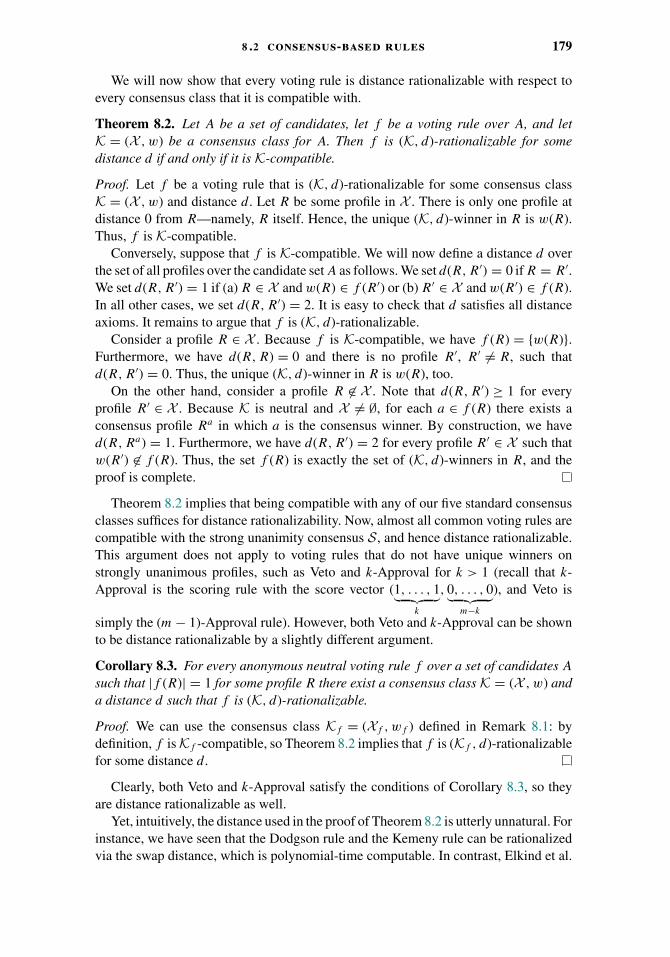
8 .2 consensus-based rules 179
We will now show that every voting rule is distance rationalizable with respect toevery consensus class that it is compatible with.
Theorem 8.2. Let A be a set of candidates, let f be a voting rule over A, and letK = (X , w) be a consensus class for A. Then f is (K, d)-rationalizable for somedistance d if and only if it is K-compatible.
Proof. Let f be a voting rule that is (K, d)-rationalizable for some consensus classK = (X , w) and distance d. Let R be some profile in X . There is only one profile atdistance 0 from R—namely, R itself. Hence, the unique (K, d)-winner in R is w(R).Thus, f is K-compatible.
Conversely, suppose that f is K-compatible. We will now define a distance d overthe set of all profiles over the candidate set A as follows. We set d(R, R′) = 0 if R = R′.We set d(R, R′) = 1 if (a) R ∈ X and w(R) ∈ f (R′) or (b) R′ ∈ X and w(R′) ∈ f (R).In all other cases, we set d(R, R′) = 2. It is easy to check that d satisfies all distanceaxioms. It remains to argue that f is (K, d)-rationalizable.
Consider a profile R ∈ X . Because f is K-compatible, we have f (R) = {w(R)}.Furthermore, we have d(R, R) = 0 and there is no profile R′, R′ �= R, such thatd(R, R′) = 0. Thus, the unique (K, d)-winner in R is w(R), too.
On the other hand, consider a profile R �∈ X . Note that d(R, R′) ≥ 1 for everyprofile R′ ∈ X . Because K is neutral and X �= ∅, for each a ∈ f (R) there exists aconsensus profile Ra in which a is the consensus winner. By construction, we haved(R, Ra) = 1. Furthermore, we have d(R, R′) = 2 for every profile R′ ∈ X such thatw(R′) �∈ f (R). Thus, the set f (R) is exactly the set of (K, d)-winners in R, and theproof is complete.
Theorem 8.2 implies that being compatible with any of our five standard consensusclasses suffices for distance rationalizability. Now, almost all common voting rules arecompatible with the strong unanimity consensus S , and hence distance rationalizable.This argument does not apply to voting rules that do not have unique winners onstrongly unanimous profiles, such as Veto and k-Approval for k > 1 (recall that k-Approval is the scoring rule with the score vector (1, . . . , 1︸ ︷︷ ︸
k
, 0, . . . , 0︸ ︷︷ ︸m−k
), and Veto is
simply the (m − 1)-Approval rule). However, both Veto and k-Approval can be shownto be distance rationalizable by a slightly different argument.
Corollary 8.3. For every anonymous neutral voting rule f over a set of candidates A
such that |f (R)| = 1 for some profile R there exist a consensus class K = (X , w) anda distance d such that f is (K, d)-rationalizable.
Proof. We can use the consensus class Kf = (Xf , wf ) defined in Remark 8.1: bydefinition, f is Kf -compatible, so Theorem 8.2 implies that f is (Kf , d)-rationalizablefor some distance d.
Clearly, both Veto and k-Approval satisfy the conditions of Corollary 8.3, so theyare distance rationalizable as well.
Yet, intuitively, the distance used in the proof of Theorem 8.2 is utterly unnatural. Forinstance, we have seen that the Dodgson rule and the Kemeny rule can be rationalizedvia the swap distance, which is polynomial-time computable. In contrast, Elkind et al.
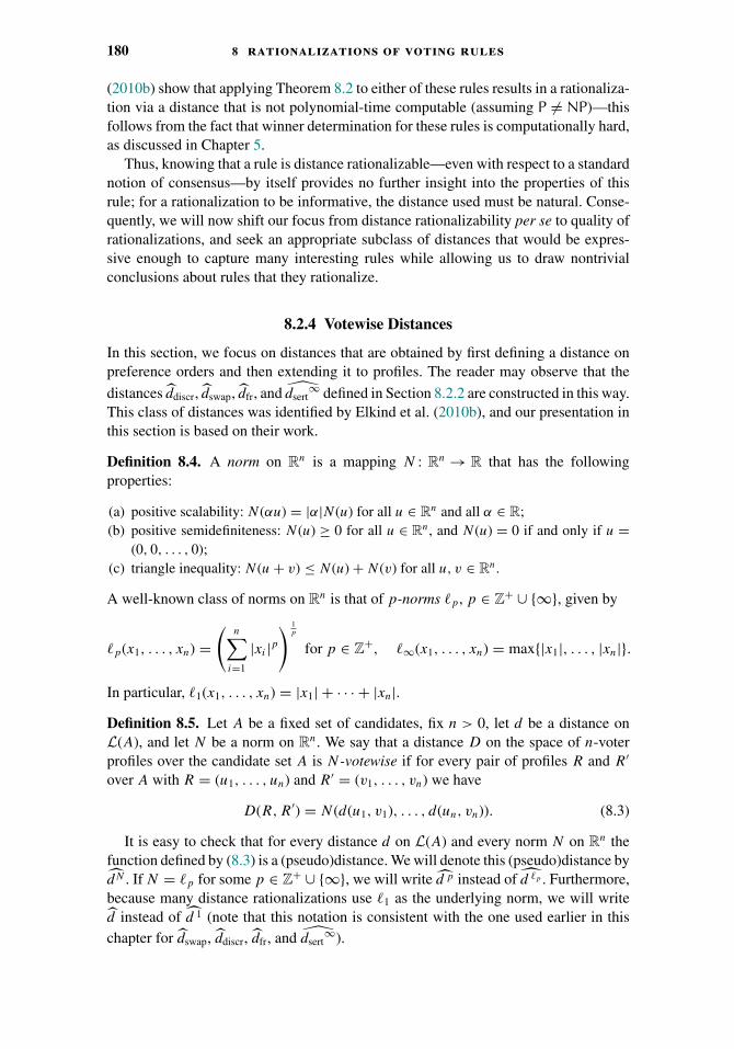
180 8 rationalizations of voting rules
(2010b) show that applying Theorem 8.2 to either of these rules results in a rationaliza-tion via a distance that is not polynomial-time computable (assuming P �= NP)—thisfollows from the fact that winner determination for these rules is computationally hard,as discussed in Chapter 5.
Thus, knowing that a rule is distance rationalizable—even with respect to a standardnotion of consensus—by itself provides no further insight into the properties of thisrule; for a rationalization to be informative, the distance used must be natural. Conse-quently, we will now shift our focus from distance rationalizability per se to quality ofrationalizations, and seek an appropriate subclass of distances that would be expres-sive enough to capture many interesting rules while allowing us to draw nontrivialconclusions about rules that they rationalize.
8.2.4 Votewise Distances
In this section, we focus on distances that are obtained by first defining a distance onpreference orders and then extending it to profiles. The reader may observe that the
distances ddiscr, dswap, dfr, and dsert∞ defined in Section 8.2.2 are constructed in this way.
This class of distances was identified by Elkind et al. (2010b), and our presentation inthis section is based on their work.
Definition 8.4. A norm on Rn is a mapping N : Rn → R that has the followingproperties:
(a) positive scalability: N (αu) = |α|N (u) for all u ∈ Rn and all α ∈ R;(b) positive semidefiniteness: N (u) ≥ 0 for all u ∈ Rn, and N (u) = 0 if and only if u =
(0, 0, . . . , 0);(c) triangle inequality: N (u + v) ≤ N (u) + N (v) for all u, v ∈ Rn.
A well-known class of norms on Rn is that of p-norms p, p ∈ Z+ ∪ {∞}, given by
p(x1, . . . , xn) =(
n∑i=1
|xi |p) 1
p
for p ∈ Z+, ∞(x1, . . . , xn) = max{|x1|, . . . , |xn|}.
In particular, 1(x1, . . . , xn) = |x1| + · · · + |xn|.Definition 8.5. Let A be a fixed set of candidates, fix n > 0, let d be a distance onL(A), and let N be a norm on Rn. We say that a distance D on the space of n-voterprofiles over the candidate set A is N-votewise if for every pair of profiles R and R′
over A with R = (u1, . . . , un) and R′ = (v1, . . . , vn) we have
D(R, R′) = N(d(u1, v1), . . . , d(un, vn)). (8.3)
It is easy to check that for every distance d on L(A) and every norm N on Rn thefunction defined by (8.3) is a (pseudo)distance. We will denote this (pseudo)distance bydN . If N = p for some p ∈ Z+ ∪ {∞}, we will write d p instead of d p . Furthermore,because many distance rationalizations use 1 as the underlying norm, we will writed instead of d 1 (note that this notation is consistent with the one used earlier in thischapter for dswap, ddiscr, dfr, and dsert
∞).
8 .2 consensus-based rules 181
Given a norm N , we say that a rule is N -votewise if it can be distance rationalizedvia an N-votewise distance; we say that a rule is votewise if it is N-votewise for somenorm N .
Votewise distances are expressive enough to rationalize many classic voting rules.For instance, the rationalizations of the Dodgson rule, the Kemeny rule, Plurality,and the Borda rule described in Section 8.2.1 demonstrate that all these rules are 1-votewise, and the results of Lerer and Nitzan (1985) and Elkind et al. (2009a, 2010b)imply that the class of votewise rules includes essentially all scoring rules,3 a simplifiedversion of the Bucklin rule, and several other less common voting rules.
We will now demonstrate that votewise rules have a number of desirable properties,both from a normative and from a computational perspective.
Normative Properties of Votewise Rules
An important feature of the votewise distance rationalizability framework is that onecan derive properties of votewise rules from the properties of their components, thatis, the underlying distance on votes, the norm, and the consensus class. Elkind et al.(2010b, 2011b) consider such classic normative properties of voting rules as anonymity,neutrality, continuity, consistency, homogeneity and monotonicity, and, for each ofthem, derive sufficient conditions on the components of a votewise rationalization forthe resulting rule to have the respective property. We present a sample of these resultsin the following.
Anonymity. Recall that a voting rule is said to be anonymous if its result does notchange when the ballots are permuted. It turns out that anonymity of a votewise ruleis inherited from the corresponding norm. Specifically, a norm N on Rn is said to besymmetric if it satisfies N(x1, . . . , xn) = N(xσ (1), . . . , xσ (n)) for every permutation σ
of {1, . . . , n}; note that all p-norms are symmetric. Elkind et al. (2010b) show thefollowing easy result.
Proposition 8.4. Suppose that a voting rule f is (K, dN )-rationalizable for somepseudodistance d over L(A), a consensus class K, and a symmetric norm N . Then f
is anonymous.
Neutrality. A voting rule is said to be neutral if its result does not depend on thecandidates’ names. Neutrality of a votewise rule is a property of the underlying distanceon votes. Namely, a distance d on L(A) is said to be neutral if for every permutationπ : A → A and every pair of votes u, v ∈ L(A) it holds that d(u, v) = d(u′, v′) whereu′ and v′ are obtained from, respectively, u and v by renaming the candidates accordingto π . The following proposition is due to Elkind et al. (2010b).
Proposition 8.5. Suppose that a voting rule f is (K, dN )-rationalizable for some normN , a consensus class K, and a neutral pseudodistance d over L(A). Then f is neutral.
Consistency. A voting rule f is said to be consistent if for every pair of profilesR1, R2 such that f (R1) ∩ f (R2) �= ∅, the preference profile R1 + R2 obtained by
3 The exceptions are rules like Veto, which are not compatible with any standard consensus class; however, evensuch rules are votewise rationalizable via a pseudodistance.
182 8 rationalizations of voting rules
concatenating R1 and R2 satisfies f (R1 + R2) = f (R1) ∩ f (R2). Consistency is a verydemanding property: while all common voting rules are anonymous and neutral, theclass of voting rules that are anonymous, neutral and consistent consists of compositionsof scoring rules (Young, 1975). Nevertheless, Elkind et al. (2010b) obtain a sufficientcondition for a distance rationalizable voting rule to be consistent.
Proposition 8.6. Suppose that a voting rule f is (U , d p)-rationalizable for somep ∈ Z+ and some pseudodistance d over L(A). Then f is consistent.
Homogeneity. A voting rule f is said to be homogeneous if for every profile R andevery positive integer k it holds that f (R) = f (kR), where kR is the preference profileobtained by concatenating k copies of R. This notion can be seen as a relaxation ofthe notion of consistency. Elkind et al. (2011b) present several sufficient conditions forhomogeneity of a votewise rule. For instance, they show that many of the voting rulesthat can be rationalized via the ∞ norm are homogeneous.
Proposition 8.7. Suppose that a voting rule f is (K, d∞)-rationalizable for somepseudodistance d over L(A) and a consensus class K ∈ {S,U ,M}. Then f is homo-geneous.
Monotonicity. A voting rule f is said to be monotone if moving a winning candidateupward in some voters’ preference orders (without changing the relative order of othercandidates) does not make him a loser. To identify sufficient conditions for monotonicityof a votewise rule, Elkind et al. (2011b) introduce several notions of monotonicity fordistances over votes. In particular, they define relatively monotone distances. These arethe distances over L(A) such that for every candidate a ∈ A the following conditionholds. Suppose that we have:
(i) two votes y, y ′ ∈ L(A) such that y and y ′ rank all candidates in A \ {a} in the sameorder, but y ′ ranks a higher than y does, and
(ii) two votes x, z ∈ L(A) such that x ranks a first and z does not.
Then
d(x, y) − d(x, y ′) � d(z, y) − d(z, y ′). (8.4)
Elkind et al. (2011b) show that the relative monotonicity condition is satisfied by theswap distance. Moreover, they prove the following result.
Proposition 8.8. Suppose that a voting rule f is (K, d)-rationalizable for some rel-atively monotone distance d over L(A) and a consensus class K ∈ {S,U}. Then f ismonotone.
Algorithmic Properties of Votewise Rules
Votewise rules are also appealing from a complexity-theoretic perspective: it turns outthat we can show tractability results for them under a mild condition on the underlyingdistance. For the definitions of the complexity classes mentioned in this section, werefer the reader to the book of Hemaspaandra and Ogihara (2002).
8 .2 consensus-based rules 183
Definition 8.6. We say that a distance D on the space of profiles over a candidate setA is normal if:
(a) D is polynomial-time computable;(b) D takes values in the set Z+ ∪ {+∞};(c) if R1 and R2 have a different number of votes, then D(R1, R2) = +∞.
Given a voting rule f , we consider the problem of determining whether a givencandidate is one of the winners in a given profile under f ; we refer to this problem asf -Winner. Elkind et al. (2010b) show the following set of results for this problem.Suppose that a voting rule f is (K, D)-rationalizable for some normal distance D anda consensus class K ∈ {S,U ,M, C}. Then:
(i) f -Winner is in PNP;(ii) if there exists a polynomial p such that for every pair of n-voter m-candidate profiles
R1, R2 it holds that D(R1, R2) ≤ p(m + n), then f -Winner is in �p2 ;
(iii) if there exists a distance on votes d such that D = d, then f -Winner is fixed-parametertractable with respect to the number of candidates;
(iv) if there exists a distance on votes d such that D = d or D = d∞, K ∈ {U ,M}, and D
is neutral, then f -Winner is in P/poly.
The first two results extend to the transitivity consensus T (which was not consideredby Elkind et al. (2010b)); note also that for these results the distance D is not requiredto be votewise. However, it is not clear if the FPT algorithm in (iii) can be extended toT as well.
We emphasize that it is not the case that for every votewise rule the winner deter-mination problem is in P (unless P = NP). In fact f -Winner may be intractable evenif f is 1-votewise rationalizable with respect to a standard consensus class via aneasy-to-compute distance on votes: examples are provided by the Dodgson rule andthe Kemeny rule, which are known to be computationally hard (Hemaspaandra et al.,1997a, 2005).
Votewise Distances: Discussion
We have seen that many common voting rules admit votewise distance rationaliza-tions, and that distance rationalizable voting rules have several desirable properties.On the other hand, the “trivial” distance rationalization presented in Theorem 8.2is clearly not votewise. Furthermore, some voting rules (most notably, STV) can beshown not to admit a votewise distance rationalization with respect to the standardconsensus classes (Elkind et al., 2010a); we remark that the known distance rational-ization for STV (Meskanen and Nurmi, 2008) is rather complex. Thus, the concept ofa votewise distance appears to be useful for distinguishing between “good” and “bad”rationalizations.
Note, however, that the rationalizations of the Copeland rule and Maximin givenin Section 8.2.1 are not votewise, despite being quite simple and intuitive. In fact, itis not known whether these rules are votewise distance rationalizable. It remains achallenge to come up with a definition of a “good” distance rationalization that covers
184 8 rationalizations of voting rules
all intuitively appealing rationalizations, but excludes the rationalization described inTheorem 8.2.
8.3 Rules as Maximum Likelihood Estimators
We will now turn our attention to voting rules that can be represented as maximumlikelihood estimators. We start by revisiting the probabilistic model put forward byCondorcet (1785), and its interpretation by Young (1988).
Briefly, the basic assumption of Condorcet’s model is that there always exists acorrect ranking of the alternatives, which, however, cannot be observed directly. Votersderive their preferences over the alternatives from this ranking: when comparing twoalternatives, each voter is more likely to make the correct judgment than the incorrectone. Moreover, voters make their decisions independently from each other, and a priorieach ranking is equally likely to be correct.
Formalizing Condorcet’s ideas turned out to be a challenging task; in what follows,we discuss some of the reasons for this. However, from a historical perspective, hisideas are very important, as they represent one of the earliest applications of whatis now known as the maximum likelihood estimation approach. Under this approach,one computes the likelihood of the given preference profile for each possible “stateof the world,” that is, the true ranking of the alternatives. The best ranking(s) of thealternatives are then the one(s) that have the highest likelihood of producing the givenprofile. If we assume a uniform prior over the space of all possible rankings, thisprocedure can be interpreted as estimating the most likely state of the world given thepreference data (the equivalence of the two interpretations follows immediately fromthe Bayes rule).
Condorcet’s approach can be extended in two different directions: First, we canconsider different noise models, that is, ways in which voters’ preferences may arisefrom the true state of the world. Second, instead of associating a state of the worldwith a ranking of the alternatives, we can associate it with the identity of the bestalternative (or, more generally, a set of pairwise comparisons between the alternatives);this approach is particularly attractive if the goal is to determine a single election winnerrather than a full ranking of the alternatives (and in particular if there is indeed a unique“correct solution” to the decision problem at hand). In what follows, we survey recentresearch that explores these directions.
8.3.1 Two Alternatives: Condorcet Jury Theorem
When there are only two alternatives to choose from, it is natural to use majority voting,that is, select an alternative that is supported by at least half of the voters (breakingties arbitrarily). It turns out that this is also the right strategy in Condorcet’s model; infact, as the number of voters grows, the probability that majority voting identifies thebetter alternative approaches 1. This result is known as the Condorcet Jury Theorem,and dates back to the original paper of Condorcet (1785).
Theorem 8.9. Suppose that |A| = 2, and a priori each of the alternatives in A isequally likely to be the better choice. Suppose also that there are n voters, and each voter

8 .3 rules as maximum likelihood estimators 185
correctly identifies the better alternative with probability p, 1/2 < p ≤ 1; further, eachvoter makes her judgment independently from the other voters. Then the probabilitythat the group makes the correct decision using the simple majority rule approaches 1as n → +∞.
Theorem 8.9 follows immediately from the Chernoff bound (see, e.g., Alon andSpencer, 2008); Condorcet’s proof was based on a direct combinatorial argument.
Theorem 8.9 can be extended in a variety of ways. For instance, it can be generalizedto the case where voters are a priori not identical, that is, voter i’s probability to makethe correct choice is pi and not all pis are equal: Nitzan and Paroush (1982) andShapley and Grofman (1984) show that in this case it is optimal to use weighted voting,assigning a weight of log pi
1−pito voter i. However, in practice the probabilities pi are
often not known; to mitigate this, Baharad et al. (2011, 2012) propose a procedure forestimating them. Other extensions deal with settings where voters are not independent(see, e.g., Shapley and Grofman, 1984; Berg, 1993a, 1993b; Ladha, 1992, 1993, 1995;Dietrich and List, 2004) or strategic (Austen-Banks and Smith, 1994; McLennan, 1998;Peleg and Zamir, 2012), or a priori the alternatives are not symmetric and the voters’probabilities of making the correct choice depend on the state of nature (Ben-Yasharand Nitzan, 1997).
When |A| > 2, the analysis becomes more complicated. In particular, it depends onwhether the goal is to identify the most likely ranking of alternatives or the alternativethat is most likely to be ranked first. We will now consider both of these options,starting with the former.
8.3.2 Condorcet’s Model and Its Refinements
In his original paper, Condorcet made the following assumptions.
(1) In every pairwise comparison each voter chooses the better alternative with some fixedprobability p, where 1/2 < p ≤ 1.
(2) Each voter’s judgment on every pair of alternatives is independent of her judgment onevery other pair.
(3) Each voter’s judgment is independent of the other voters’ judgments.(4) Each voter’s judgment produces a ranking of the alternatives.
However, assumptions (2) and (4) are incompatible. Indeed, if a voter ranks everypair of alternatives correctly with some fixed probability, then she may end up witha nontransitive judgment, which is prohibited by (4). In other words, if we insist thatvoters always produce a linear order as their judgment, then their judgments on differentpairs of alternatives are no longer independent.
There are two differing opinions on how exactly Condorcet’s model should beunderstood. Some believe that we should allow intransitive preferences, arguing thatthe vote is not really a preference, but rather the voter’s best approximation to thecorrect ranking as she perceives it. It may happen that the best approximation is in factintransitive (see, e.g., Truchon, 2008); however, it cannot be ignored, as it providesuseful information.
186 8 rationalizations of voting rules
Another interpretation of Condorcet’s proposal is as follows: a voter forms heropinion by considering pairs of alternatives independently, but if the result happens tobe intransitive, she discards it and tries to form her opinion again until a valid (acyclic)preference order is obtained. In statistics, the resulting probabilistic model is knownas the Mallows noise model (Mallows, 1957). Note, however, that this model violatescondition (2) (see, e.g., Gordon and Truchon, 2008).
Commenting on Condorcet’s writings, Young (1988) wrote: “One must admit thatthe specific probabilistic model by which Condorcet reached his conclusions is almostcertainly not correct in its details.” He went further to say that the plausibility of anysolution based on Condorcet’s ideas must therefore be subjected to other tests. However,he went on and developed Condorcet’s framework to see what Condorcet would haveobtained if he possessed the necessary technical skills to perform his analysis tothe end. We will now present Young’s analysis, together with some refinements andextensions.
8.3.3 MLE for Choosing a Ranking
In this section, we describe an MLE approach to selecting the best ranking(s) of thealternatives. Recall that a social preference function is a mapping that given a listof rankings of the alternatives outputs a nonempty set of aggregate rankings; thus,in this section we focus on representing social preference functions within the MLEframework.
We start by presenting Young’s analysis of Condorcet’s proposal (see Young, 1988),followed by a discussion of a more general approach put forward by Conitzer andSandholm (2005a) and Conitzer et al. (2009b).
Let u ∈ L(A) be the true state of the world, and let v ∈ L(A) be some rankingthat agrees with u on k pairs of alternatives. Note that we have dswap(v, u) = (
m2
)− k.Then under both interpretations of Condorcet’s model discussed in Section 8.3.2 theprobability that a voter forms opinion v is proportional to
pk(1 − p)(m2)−k = p(m
2)−dswap(v,u)(1 − p)dswap(v,u).
If each voter forms her opinion independently from other voters, the probability ofa profile (v1, . . . , vn) given that u is the true state of the world is proportional to
n∏i=1
(p
1 − p
)−dswap(vi ,u)
=(
p
1 − p
)−∑ni=1 dswap(vi ,u)
.
If each state of the world is a priori considered equally likely, the rankings that are mostlikely to be correct are the ones that maximize the probability of the observed data, or,equivalently, minimize
∑ni=1 dswap(vi, u) (note that p > 1/2 and hence p
1−p> 1). Thus,
Condorcet’s approach results in a social preference function fCond that given a profileR = (v1, . . . , vn) over a candidate set A, outputs the set argminu∈L(A)
∑ni=1 dswap(vi, u).
This is exactly the social preference function associated with the Kemeny rule (seeSection 8.2.1).

8 .3 rules as maximum likelihood estimators 187
General r-Noise Models
Young’s analysis is based on a specific noise model, that is, a way voters’ judgments areformed given an underlying state of the world. By considering other noise models, wecan obtain other social preference functions. To pursue this agenda, we need a formaldefinition of a noise model.
Definition 8.7. A noise model for rankings, or an r-noise model, over a candidate setA is a family of probability distributions P(· | u)u∈L(A) on L(A). For a given u ∈ L(A),P(v | u) is the probability that a voter forms a preference order v when the correctranking is u.
We emphasize that the parameters of a noise model are assumed to be the same forall voters and do not depend on the number of voters. That is, we think of voters asindependent agents that are influenced by the same factors in the same way.
Example 8.10. The Mallows model (Mallows, 1957) is a family of r-noise models(Pdswap,p
)1/2<p<1
given by
Pdswap,p(v | u) = 1
μp
ϕ−dswap(v,u), where ϕ = p
1 − pand μp =
∑v∈L(A)
ϕ−dswap(v,u).
Here, μp is the normalization constant; because dswap is a neutral distance, the value ofμp does not depend on the choice of u (Mallows, 1957).
Under the MLE approach, every r-noise model leads to a social preference function.
Definition 8.8. A social preference function f over A is the maximum likelihoodestimator (MLE) for an r-noise model P over A if for every positive integer n andevery n-voter profile R = (v1, . . . , vn) it holds that
f (R) = argmaxu∈L(A)
n∏i=1
P(vi | u).
A very general method of constructing r-noise models was proposed by Conitzeret al. (2009b), who introduced the notion of a simple ranking scoring function.
Definition 8.9. A social preference function f over A is said to be a simple rankingscoring function (SRSF) if there exists a mapping ρ : L(A) × L(A) → R such that forevery positive integer n and every n-voter profile R = (v1, . . . , vn) it holds that
f (R) = argmaxu∈L(A)
n∑i=1
ρ(vi, u). (8.5)
Intuitively, ρ(v, u) assigns a score to v based on the similarity between v and u,and f chooses u so as to maximize the total score of the given profile. We say thata mapping ρ : L(A) × L(A) → R is neutral if ρ(v′, u′) = ρ(v, u), where rankings v′
and u′ are obtained by renaming alternatives in v and u according to some permutationπ : A → A. Conitzer et al. (2009b) show that a simple ranking scoring function f isneutral if and only if there exists a neutral mapping ρ satisfying (8.5).
188 8 rationalizations of voting rules
Example 8.11. Every distance d on L(A) defines a simple ranking scoring function:we can set ρ(v, u) = −d(v, u). The corresponding social preference function mapsa profile R = (v1, . . . , vn) to the set of rankings argminu∈L(A)
∑ni=1 d(vi, u). Observe
that this social preference function is closely related to the voting rule that is distancerationalizable via d and the strong unanimity consensus S .
Every SRSF corresponds to an infinite family of r-noise models: If f is the SRSFdefined by a mapping ρ, then for every ϕ ∈ (1,+∞) we can set
Pρ,ϕ(v | u) = 1
μρ,ϕ,u
ϕ ρ(v,u), where μρ,ϕ,u =∑
v∈L(A)
ϕ ρ(v,u); (8.6)
Conitzer et al. (2009b) use ϕ = 2 in their paper. By construction, f is the maximumlikelihood estimator for Pρ,ϕ for every ϕ ∈ (1,+∞).
Conitzer et al. (2009b) show that for social preference functions that are neutral(i.e., their output does not depend on the names of the candidates) the converse is alsotrue. More precisely, they prove the following characterization result.
Theorem 8.12. A neutral social preference function is an MLE if and only if it is anSRSF.
Theorem 8.12 provides a convenient way to show that a given social preferencefunction f is an MLE: it suffices to exhibit a mapping ρ witnessing that f is an SRSF.Conitzer et al. (2009b) apply this method to show that for every score vector α =(α1, . . . , αm) the corresponding social preference function fα is an MLE. In the rest ofthis section, we give a sketch of their argument.
Recall that fα is the social preference function that orders the candidates by theirα-scores, where the α-score of a candidate a in a profile R = (v1, . . . , vn) is givenby sα(R, a) = ∑n
i=1 αpos(vi ,a); if some candidates have the same score, fα outputs allrankings that can be obtained by breaking such ties in some way.
To show that fα is an SRSF, let β1, . . . , βm be a monotonically decreasing sequence(e.g., we can take βj = m − j ), and set
ρα(v, u) =∑a∈A
βpos(u,a)αpos(v,a), (8.7)
We claim that fα is the simple ranking scoring function that corresponds to ρα . Indeed,for a given profile R = (v1, . . . , vn) we obtain
n∑i=1
ρα(vi, u) =∑a∈A
βpos(u,a)
(n∑
i=1
αpos(vi ,a)
)=∑a∈A
βpos(u,a)sα(R, a).
Thus, for u to maximize the expression∑n
i=1 ρα(vi, u), we should have βpos(u,a) >
βpos(u,b) (and hence pos(u, a) < pos(u, b)) whenever sα(R, a) > sα(R, b), that is, u
orders the candidates by their α-score from the highest to the lowest, breaking tiesarbitrarily. Theorem 8.12 then implies the following corollary.
Corollary 8.13. The social preference function fα is an MLE.
8 .3 rules as maximum likelihood estimators 189
8.3.4 MLE for Choosing a Winner
In the previous section we described an MLE approach to selecting the best ranking(s).However, typically our goal is to select a single winner (or possibly a set of winners)rather than a ranking of the candidates. To extend the MLE framework to this setting,we can simply output the top candidate(s) in the best ranking(s). Alternatively, we canestimate the likelihood that a given candidate is the best. To this end, for each candidatewe determine the total probability mass (with respect to the uniform distribution) ofthe rankings where she is the top choice, and output the candidate(s) that maximize thisquantity; the validity of this method follows from the Bayes rule. We will now discussthese approaches in more detail.
Deducing Winners from Rankings: MLERIV Rules
In Section 8.2.1 we transformed the social preference function associated with theKemeny rule into a voting rule, by picking the top candidate in each ranking output bythis social preference function. By extending this procedure to arbitrary MLE socialpreference functions, we obtain a class of rules known as MLERIV (Conitzer andSandholm, 2005a).
Definition 8.10. Let f be a social preference function that is MLE for an r-noise modelP . Let f be a voting rule defined by f (R) = {top(u) | u ∈ f (R)}, where top(u) denotesthe top candidate in ranking u. This rule is called the maximum likelihood estimatorfor ranking under identically distributed independent votes (MLERIV) for P .
According to Definition 8.10, the Kemeny rule is MLERIV for the Mallows noisemodel. Another family of MLERIV rules is provided by Example 8.11: Theorem 8.12implies that for every neutral distance d over L(A) the (S, d)-rationalizable voting ruleis MLERIV. Furthermore, Corollary 8.13 implies that every scoring rule is MLERIV.
Estimating the Winners: Young’s Interpretation of Condorcet’s Proposal
The MLERIV-based approach provides a simple way to cast many voting rules withinthe MLE framework. However, it is not appropriate if our goal is to output the candidatethat is most likely to be ranked first. Indeed, under an r-noise model the probabilitythat a candidate is ranked first in the true ranking is obtained by adding together theprobabilities of all rankings where she appears on top, and it is entirely possible that thetop candidate in the most likely ranking is a, but the cumulative probability of rankingsthat have a on top is lower than the cumulative probability of rankings that have someother candidate b on top.
This was clearly understood by Condorcet himself, who probably did not have thetechnical skills to pursue this line of reasoning. Young (1988) argues that this approachwould lead him to the Borda rule, at least when p is sufficiently close to 1/2. Youngalso speculates on reasons why Condorcet might have chosen to abandon this trainof thought (see Young, 1988, for an amusing account of the relationship betweenCondorcet and Borda).
190 8 rationalizations of voting rules
We will now present Young’s extension of Condorcet’s analysis. While it aims toestimate the most likely winner under the Mallows model, it makes the simplifyingassumption that in the prior distribution over the states of the world all pairwisecomparisons between the alternatives are independent from each other. For the Mallowsmodel this assumption is not true: if A = {a, b, c} and the prior distribution over thestates of the world is uniform over L(A), knowing that in the true state of the world a
is ranked above b influences our beliefs about the outcome of the comparison betweena and c. Thus, Young’s analysis can be seen as a heuristic algorithm for computing themost likely winner; later, we will see that its output may differ from that of the exactalgorithm (see also Xia, 2014a).
Given a pair of candidates a, b ∈ A, let nab denote the number of voters in a givenprofile (v1 . . . , vn) who prefer a to b. Let S be a fixed set of voters of size nab, andconsider the event that the voters in S prefer a to b, while the remaining voters prefer b
to a; denote this event by ES . If in the true state of the world a is preferred to b, then theprobability of ES is exactly pnab (1 − p)nba . Conversely, if in the true state of the world b
is preferred to a, then the probability of ES is (1 − p)nabpnba . The prior probability thatin the true state of the world a is preferred b is exactly 1/2. Therefore, the probabilityof the event ES is 1
2 (pnab (1 − p)nba + (1 − p)nabpnba ). Hence, by the Bayes rule, theprobability that in the true state of the world a is preferred to b is proportional to
pnab (1 − p)nba
pnab (1 − p)nba + (1 − p)nabpnba. (8.8)
To compute the probability that in the true state of the world a is preferred to everyother candidate, we take the product of probabilities (8.8) over all b �= a; note that thisstep makes use of the assumption that in the prior distribution over the states of theworld all pairwise comparisons are independent. It follows that the probability that a
is the true winner given that the observed profile is (v1, . . . , vn) is given by∏b∈A\{a}
pnab (1 − p)nba
pnab (1 − p)nba + (1 − p)nabpnba=
∏b∈A\{a}
1
1 +(
1−pp
)nab−nba.
Thus, the most likely winners are the candidates that minimize the expression
κa(ϕ) =∏
b∈A\{a}
(1 + ϕnba−nab
), where ϕ = p
1 − p. (8.9)
Now, the behavior of this expression crucially depends on the value of ϕ = p1−p
. Wewill consider two cases: (1) p is very close to 1 and hence ϕ → +∞ (i.e., a voter isalmost always right) and (2) p is very close to 1/2 and hence ϕ → 1 (a voter has onlya slight advantage over a random coin toss). We denote the corresponding voting rulesby MLE∞
intr and MLE1intr, respectively (the reasons for this notation are explained in
Remark 8.14). The following analysis is based on the work of Elkind and Shah (2014).
p → 1, ϕ → +∞. The rate of growth of κa(ϕ) as ϕ → +∞ depends on the degreeof its highest-order term, that is,
∑b∈A\{a}:nba>nab
(nba − nab): slowest-growingfunctions correspond to the most likely candidates.
Thus, to determine the MLE∞intr-winners, we first compute the score of each
candidate a ∈ A as the sum of a’s loss margins in all pairwise elections she
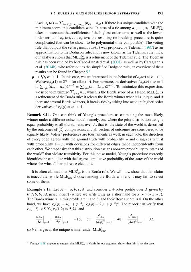
8 .3 rules as maximum likelihood estimators 191
loses: sT (a) = ∑b∈A\{a}:nba>nab
(nba − nab). If there is a unique candidate with theminimum score, this candidate wins. In case of a tie among a1, . . . , ak , MLE∞
intrtakes into account the coefficients of the highest-order terms as well as the lower-order terms of κa1 (ϕ), . . . , κak
(ϕ); the resulting tie-breaking procedure is quitecomplicated (but can be shown to be polynomial-time computable). The votingrule that outputs the set arg mina∈A sT (a) was proposed by Tideman (1987) as anapproximation to the Dodgson rule, and is now known as the Tideman rule; thus,our analysis shows that MLE∞
intr is a refinement of the Tideman rule. The Tidemanrule has been studied by McCabe-Dansted et al. (2008), as well as by Caragianniset al. (2014b), who refer to it as the simplified Dodgson rule; an overview of theirresults can be found in Chapter 5.4
p → 1/2, ϕ → 1. In this case, we are interested in the behavior of κa(ϕ) as ϕ → 1.We have κa(1) = 2m−1 for all a ∈ A. Furthermore, the derivative of κa(ϕ) at ϕ = 1is∑
c �=a(nca − nac)2m−2 = ∑c �=a(n − 2nac)2m−2. To minimize this expression,
we need to maximize∑
c �=a nac, which is the Borda score of a. Hence, MLE1intr is
a refinement of the Borda rule: it selects the Borda winner when it is unique, and ifthere are several Borda winners, it breaks ties by taking into account higher-orderderivatives of κa(ϕ) at ϕ → 1.
Remark 8.14. One can think of Young’s procedure as estimating the most likelywinner under a different noise model, namely, one where the prior distribution assignsequal probability to all tournaments over A, that is, the state of the world is describedby the outcomes of
(m2
)comparisons, and all vectors of outcomes are considered to be
equally likely. Voters’ preferences are tournaments as well; in each vote, the directionof every edge agrees with the ground truth with probability p and disagrees with itwith probability 1 − p, with decisions for different edges made independently fromeach other. We emphasize that this distribution assigns nonzero probability to “states ofthe world” that violate transitivity. For this noise model, Young’s procedure correctlyidentifies the candidate with the largest cumulative probability of the states of the worldwhere she wins all her pairwise elections.
It is often claimed that MLE1intr is the Borda rule. We will now show that this claim
is inaccurate: while MLE1intr chooses among the Borda winners, it may fail to select
some of them.
Example 8.15. Let A = {a, b, c, d} and consider a 4-voter profile over A given by(adcb, bcad, abdc, bcad) (where we write xyzt as a shorthand for x � y � z � t).The Borda winners in this profile are a and b, and their Borda score is 8. On the otherhand, we have κa(ϕ) = 4(1 + ϕ−4), κb(ϕ) = 2(1 + ϕ−2)2. The reader can verify thatκa(1.2) ≈ 5.93, κb(1.2) ≈ 5.74, and
dκa
dϕ
∣∣∣ϕ=1
= dκb
dϕ
∣∣∣ϕ=1
= −16, butd2κa
(dϕ)2
∣∣∣ϕ=1
= 48,d2κb
(dϕ)2
∣∣∣ϕ=1
= 32,
so b emerges as the unique winner under MLE1intr.
4 Young (1988) appears to suggest that MLE∞intr is Maximin; our argument shows that this is not the case.

192 8 rationalizations of voting rules
Estimating the Winners under an r-Noise Model
It is natural to ask whether we can estimate the most likely winner under the Mallowsmodel without making the simplifying assumption that in the prior distribution overthe states of the world all pairwise comparisons are independent. To the best of ourknowledge, Procaccia et al. (2012) were the first to do this for p → 1/2; their argumentextends to more general noise models and to settings where the goal is to select afixed-size subset of candidates. They have also considered the case p → 1 (see alsothe work of Elkind and Shah, 2014). Just as in Young’s analysis, the result turns out todepend on the value of p: when p → 1 (and ϕ = p
1−p→ +∞), we obtain a refinement
of the Kemeny rule, and when p → 1/2 (and ϕ → 1), we obtain a refinement of theBorda rule. We will now present the arguments both for ϕ → +∞ and for ϕ → 1; werefer to the resulting rules as MLE∞
tr and MLE1tr, respectively.
For every candidate a ∈ A let La denote the set of all rankings in L(A) where a
is ranked first. Recall that under the Mallows noise model the probability of a profile(v1, . . . , vn) given that the true state of the world is described by a ranking u isproportional to ϕ−∑n
i=1 dswap(vi ,u). Thus, to compute the most likely winner, we need tofind the candidates that maximize the expression
τa(ϕ) =∑u∈La
ϕ−∑ni=1 dswap(vi ,u).
p → 1, ϕ → +∞. The rule MLE∞tr returns a set of candidates S such that for
every a ∈ S, b ∈ A \ S we have τa(ϕ) > τb(ϕ) for all sufficiently large valuesof ϕ. To see that S is not empty, note that functions τa(ϕ), a ∈ A, are Laurentpolynomials (i.e., sums of powers of ϕ), and therefore any two of these functionseither coincide or have finitely many intersection points. Moreover, for each a ∈ A
the most significant summand of τa(ϕ) at ϕ → +∞ is
ϕ−∑ni=1 dswap(vi ,u
′), where u′ ∈ argminu∈La
n∑i=1
dswap(vi, u).
Hence, MLE∞tr is a refinement of the Kemeny rule.
p → 1/2, ϕ → 1. We have τa(1) = (m − 1)! for all a ∈ A. Furthermore, the deriva-tive of τa(ϕ) at ϕ = 1 is given by
dτa
dϕ
∣∣∣ϕ=1
= −∑u∈La
n∑i=1
dswap(vi, u) = −n∑
i=1
∑u∈La
dswap(vi, u).
It is easy to show by induction on j that if pos(vi, a) = j then we have∑u∈La
dswap(vi, u) = j (m − 1)! + Cm, where Cm is a function of m (i.e., doesnot depend on vi). As
∑ni=1(m − pos(vi, a)) is exactly the Borda score of a, it
follows that a ∈ argminc∈Adτc
dϕ
∣∣ϕ=1 if and only if a is a Borda winner. Hence,
MLE1tr is a refinement of the Borda rule. Furthermore, it can be checked that
it is distinct from the Borda rule, that is, it may fail to elect some Borda win-ners; this can happen when τa(ϕ) and τb(ϕ) are different from each other, eventhough their derivatives at ϕ = 1 coincide. Furthermore, it can also be shown that
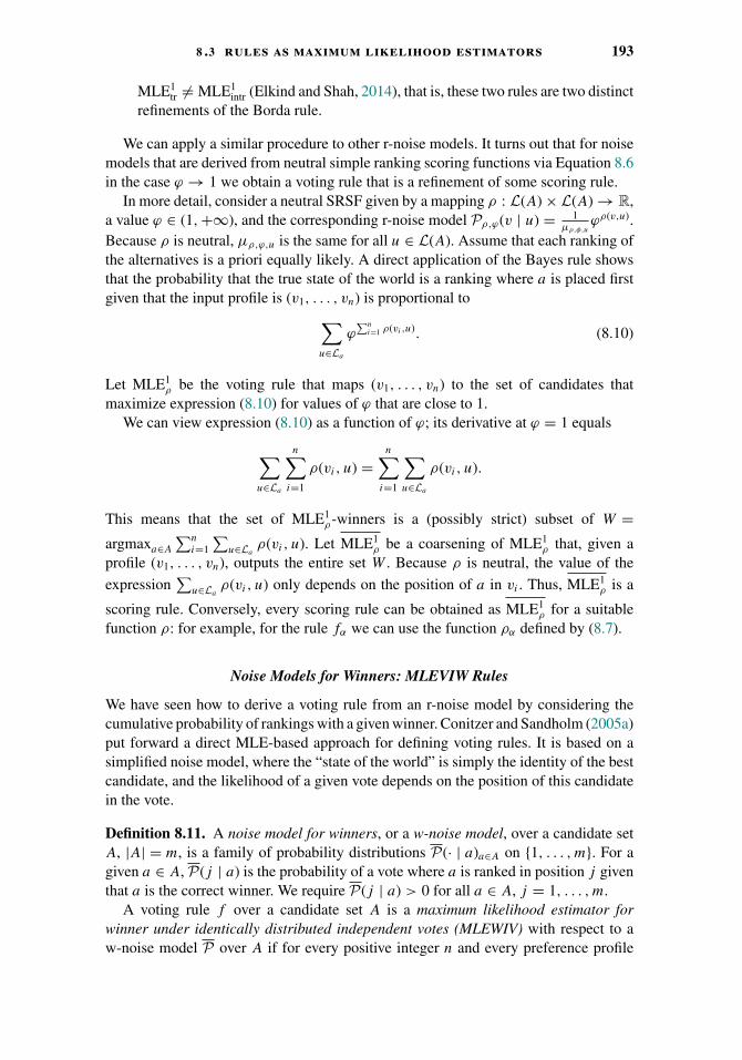
8 .3 rules as maximum likelihood estimators 193
MLE1tr �= MLE1
intr (Elkind and Shah, 2014), that is, these two rules are two distinctrefinements of the Borda rule.
We can apply a similar procedure to other r-noise models. It turns out that for noisemodels that are derived from neutral simple ranking scoring functions via Equation 8.6in the case ϕ → 1 we obtain a voting rule that is a refinement of some scoring rule.
In more detail, consider a neutral SRSF given by a mapping ρ : L(A) × L(A) → R,a value ϕ ∈ (1,+∞), and the corresponding r-noise model Pρ,ϕ(v | u) = 1
μρ,φ,uϕρ(v,u).
Because ρ is neutral, μρ,ϕ,u is the same for all u ∈ L(A). Assume that each ranking ofthe alternatives is a priori equally likely. A direct application of the Bayes rule showsthat the probability that the true state of the world is a ranking where a is placed firstgiven that the input profile is (v1, . . . , vn) is proportional to∑
u∈La
ϕ∑n
i=1 ρ(vi ,u). (8.10)
Let MLE1ρ be the voting rule that maps (v1, . . . , vn) to the set of candidates that
maximize expression (8.10) for values of ϕ that are close to 1.We can view expression (8.10) as a function of ϕ; its derivative at ϕ = 1 equals
∑u∈La
n∑i=1
ρ(vi, u) =n∑
i=1
∑u∈La
ρ(vi, u).
This means that the set of MLE1ρ-winners is a (possibly strict) subset of W =
argmaxa∈A
∑ni=1
∑u∈La
ρ(vi, u). Let MLE1ρ be a coarsening of MLE1
ρ that, given aprofile (v1, . . . , vn), outputs the entire set W . Because ρ is neutral, the value of the
expression∑
u∈Laρ(vi, u) only depends on the position of a in vi . Thus, MLE1
ρ is a
scoring rule. Conversely, every scoring rule can be obtained as MLE1ρ for a suitable
function ρ: for example, for the rule fα we can use the function ρα defined by (8.7).
Noise Models for Winners: MLEVIW Rules
We have seen how to derive a voting rule from an r-noise model by considering thecumulative probability of rankings with a given winner. Conitzer and Sandholm (2005a)put forward a direct MLE-based approach for defining voting rules. It is based on asimplified noise model, where the “state of the world” is simply the identity of the bestcandidate, and the likelihood of a given vote depends on the position of this candidatein the vote.
Definition 8.11. A noise model for winners, or a w-noise model, over a candidate setA, |A| = m, is a family of probability distributions P(· | a)a∈A on {1, . . . , m}. For agiven a ∈ A, P(j | a) is the probability of a vote where a is ranked in position j giventhat a is the correct winner. We require P(j | a) > 0 for all a ∈ A, j = 1, . . . , m.
A voting rule f over a candidate set A is a maximum likelihood estimator forwinner under identically distributed independent votes (MLEWIV) with respect to aw-noise model P over A if for every positive integer n and every preference profile
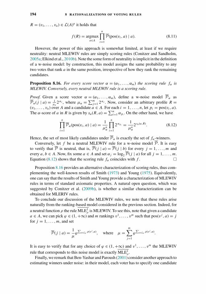
194 8 rationalizations of voting rules
R = (v1, . . . , vn) ∈ L(A)n it holds that
f (R) = argmaxa∈A
n∏i=1
P(pos(vi, a) | a). (8.11)
However, the power of this approach is somewhat limited, at least if we requireneutrality: neutral MLEWIV rules are simply scoring rules (Conitzer and Sandholm,2005a; Elkind et al., 2010b). Note the some form of neutrality is implicit in the definitionof a w-noise model: by construction, this model assigns the same probability to anytwo votes that rank a in the same position, irrespective of how they rank the remainingcandidates.
Proposition 8.16. For every score vector α = (α1, . . . , αm) the scoring rule fα isMLEWIV. Conversely, every neutral MLEWIV rule is a scoring rule.
Proof. Given a score vector α = (α1, . . . , αm), define a w-noise model Pα asPα(j | a) = 1
μα2αj , where μα = ∑m
j=1 2αj . Now, consider an arbitrary profile R =(v1, . . . , vn) over A and a candidate a ∈ A. For each i = 1, . . . , n, let pi = pos(vi, a).The α-score of a in R is given by sα(R, a) = ∑n
i=1 αpi. On the other hand, we have
n∏i=1
Pα(pos(vi, a) | a) = 1
μnα
n∏i=1
2αpi = 1
μnα
2 sα(a,R). (8.12)
Hence, the set of most likely candidates under Pα is exactly the set of fα-winners.Conversely, let f be a neutral MLEWIV rule for a w-noise model P . It is easy
to verify that P is neutral, that is, P(j | a) = P(j | b) for every j = 1, . . . , m andevery a, b ∈ A. Now, fix some a ∈ A and set αj = log2 P(j | a) for all j = 1, . . . , m.Equation (8.12) shows that the scoring rule fα coincides with f .
Proposition 8.16 provides an alternative characterization of scoring rules, thus com-plementing the well-known results of Smith (1973) and Young (1975). Equivalently,one can say that the results of Smith and Young provide a characterization of MLEWIVrules in terms of standard axiomatic properties. A natural open question, which wassuggested by Conitzer et al. (2009b), is whether a similar characterization can beobtained for MLERIV rules.
To conclude our discussion of the MLEWIV rules, we note that these rules arisenaturally from the ranking-based model considered in the previous section. Indeed, for
a neutral function ρ the rule MLE1ρ is MLEWIV. To see this, note that given a candidate
a ∈ A, we can pick ϕ ∈ (1,+∞) and m rankings v1, . . . , vm such that pos(vj , a) = j
for j = 1, . . . , m, and set
P(j | a) = 1
μϕ∑
u∈Laρ(vj ,u), where μ =
m∑j=1
ϕ∑
u∈Laρ(vj ,u).
It is easy to verify that for any choice of ϕ ∈ (1,+∞) and v1, . . . , vm the MLEWIV
rule that corresponds to this noise model is exactly MLE1ρ .
Finally, we remark that Ben-Yashar and Paroush (2001) consider another approach toestimating winners under noise: in their model, each voter has to specify one candidate
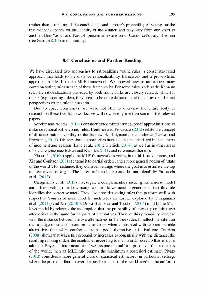
8 .4 conclusions and further reading 195
(rather than a ranking of the candidates), and a voter’s probability of voting for thetrue winner depends on the identity of the winner, and may vary from one voter toanother. Ben-Yashar and Paroush present an extension of Condorcet’s Jury Theorem(see Section 8.3.1) to this setting.
8.4 Conclusions and Further Reading
We have discussed two approaches to rationalizing voting rules: a consensus-basedapproach that leads to the distance rationalizability framework and a probabilisticapproach that leads to the MLE framework. We showed how to rationalize manycommon voting rules in each of these frameworks. For some rules, such as the Kemenyrule, the rationalizations provided by both frameworks are closely related, while forothers (e.g., scoring rules), they seem to be quite different, and thus provide differentperspectives on the rule in question.
Due to space constraints, we were not able to overview the entire body ofresearch on these two frameworks; we will now briefly mention some of the relevantpapers.
Service and Adams (2012a) consider randomized strategyproof approximations todistance rationalizable voting rules. Boutilier and Procaccia (2012) relate the conceptof distance rationalizability to the framework of dynamic social choice (Parkes andProcaccia, 2013). Distance-based approaches have also been considered in the contextof judgment aggregation (Lang et al., 2011; Dietrich, 2014), as well as in other areasof social choice (see Eckert and Klamler, 2011, and references therein).
Xia et al. (2010a) apply the MLE framework to voting in multi-issue domains, andXia and Conitzer (2011b) extend it to partial orders, and a more general notion of “stateof the world”; for instance, they consider settings where the goal is to estimate the topk alternatives for k ≥ 1. The latter problem is explored in more detail by Procacciaet al. (2012).
Caragiannis et al. (2013) investigate a complementary issue: given a noise modeland a fixed voting rule, how many samples do we need to generate so that this ruleidentifies the correct winner? They also consider voting rules that perform well withrespect to families of noise models; such rules are further explored by Caragianniset al. (2014a) and Xia (2014b). Drissi-Bakhkhat and Truchon (2004) modify the Mal-lows model by relaxing the assumption that the probability of correctly ordering twoalternatives is the same for all pairs of alternatives. They let this probability increasewith the distance between the two alternatives in the true order, to reflect the intuitionthat a judge or voter is more prone to errors when confronted with two comparablealternatives than when confronted with a good alternative and a bad one. Truchon(2008) shows that when this probability increases exponentially with the distance, theresulting ranking orders the candidates according to their Borda scores. MLE analysisadmits a Bayesian interpretation: if we assume the uniform prior over the true statesof the world, then an MLE rule outputs the maximum a posteriori estimate. Pivato(2012) considers a more general class of statistical estimators (in particular, settingswhere the prior distribution over the possible states of the world need not be uniform)

196 8 rationalizations of voting rules
and domains other than preference aggregation (including judgment aggregation andcommittee selection).
Acknowledgments
We would like to thank Shmuel Nitzan, Nisarg Shah, and the editors of this volumefor their very useful feedback, which was instrumental in improving this chapter. Weare grateful to Piotr Faliszewski for his permission to use material from our jointpapers.
CHAPTER 9
Voting in CombinatorialDomains
Jerome Lang and Lirong Xia
9.1 Motivations and Classes of Problems
This chapter addresses preference aggregation and voting on domains which are theCartesian product (or sometimes, a subset of the Cartesian product) of finite domainvalues, each corresponding to an issue, a variable, or an attribute.
As seen in other chapters of this handbook, voting rules map a profile (usually, acollection of rankings, see Chapter 1) to an alternative or a set of alternatives. A keyquestion has to do with the structure of the set of alternatives. Sometimes, this sethas a simple structure and a small cardinality (e.g., in a presidential election). But inmany contexts, it has a complex combinatorial structure. We give here three typicalexamples:
� Multiple referenda. On the day of 2012 U.S. presidential election, voters in Californiahad to decide whether to adopt each of 11 propositions.1 Five referenda were categorizedas budget/tax issues. Specifically, two of them (Propositions 30 and 38) both aimed toraise taxes for education, with different details on the type and rate of the tax. Similarly,in Florida voters had to vote on 11 propositions, eight of which were categorized asbudget/tax issues.
� Group configuration or group planning. A set of agents sometimes has to make acommon decision about a complex object, such as a common menu (composed forinstance of a first course, a main course, a dessert and a wine, with a few possible valuesfor each), or a common plan (for instance, a group of friends have to travel together toa sequence of possible locations, given some constraints on the possible sequences).
� Committee elections and more generally multiwinner elections. A set of agents has tochoose a group of delegates or representatives of some given size, from a larger set ofcandidates. As another example, a group of friends wants to choose a set of DVDs topurchase collectively, from a larger set, subject to some budget constraints.
1 http://en.wikipedia.org/wiki/California elections, November 2012.
197
198 9 voting in combinatorial domains
In these three examples, the set of alternatives has a combinatorial structure: itis a Cartesian product A = D1 × . . . × Dp, where for each i, Di is a finite valuedomain for a variable Xi , or, in the third example, a subset of a Cartesian product (seefurther). For the menu example, we may have for instance D1 = {soup, salad, quiche},D2 = {beef , salmon, tofu}, and so on. For the multiple referenda example, or moregenerally in the case of binary variables (which for the sake of simplicity we assumein most of the chapter), we write Di = {0i , 1i} for each i. Also, when all variables arebinary, we usually drop indices and parentheses: for instance, (11, 02, 13) is denotedsimply by 101.
Each of these examples has specific properties that may call for specific ways ofsolving them, which we review in this chapter. Still, the major issue for all classes ofproblems mentioned, is the trade-off between expressivity and cost. This is illustratedin the following example for multiple referenda by Lacy and Niou (2000):
Example 9.1. We have three issues, and three voters with the following preferences:
� Voter 1: 110 � 101 � 011 � 001 � 100 � 010 � 000 � 111� Voter 2: 101 � 011 � 110 � 010 � 100 � 001 � 000 � 111� Voter 3: 011 � 110 � 101 � 100 � 010 � 001 � 000 � 111
At one extreme, we can allow the voters to be fully expressive: each voter submitsa full ranking over all 23 alternatives. The number of alternatives grows exponentiallyin the number of issues, which imposes a high cognitive cost on the voters to constructtheir rankings as well as a high communication cost to report these rankings to thecentral authority that has to gather the votes and compute the outcome (cf. Chapter 10).
At the other extreme, we could ask each voter to report only her top-ranked alterna-tive. This approach is almost cost-free, but the lack of expressivity can cause seriousproblems. Applying plurality voting (see Chapter 1) for winner selection is quite arbi-trary, because three alternatives are tied in the first place by receiving a single vote.Applying the majority rule (see Chapter 1) to each issue separately, as commonly donefor multiple referenda, leads to an even worse outcome: the winner, 111, is ranked lastby all voters!
We consider separately the case where the common decision to be taken consistsof choosing the members of a committee. Benoıt and Kornhauser (1991) consider twoclasses of committee elections: designated post committees, and at-large committees.In designated post committees, candidates run for a specific post (and the size of thecommittee is the number of posts); in at-large committees, they do not run for a specificpost, and the size of the committee is specified explicitly. Designated post committeeelections are naturally expressed as elections on a combinatorial domain: variablescorrespond to posts, and the domain of each variable is the set of candidates applyingfor the post. The case of at-large elections is more subtle. An obvious choice consists inhaving binary variables corresponding to candidates, but then the cardinality constraintrestricts the set of feasible committees: we are here in a case of constrained voting on acombinatorial domain, where the set of alternatives is not simply the Cartesian productof the domains but a subset of it. Voting for at-large committees takes this cardinality
9 .1 motivations and classes of problems 199
constraint into account for restricting the set of admissible outputs2 (and, sometimes,the set of admissible inputs), and gives rise to widely used voting rules for multiwinnerelections (Brams and Fishburn, 2002).
Consider again Example 9.1. At one extreme, one could view all these domainsas ordinary domains, and proceed as usual by eliciting voters’ preferences over theset of alternatives A and then applying a given voting rule. Because the number ofalternatives grows exponentially with the number of variables, this is unrealistic assoon as one has more than a few variables; we can definitely not expect individualsto spend hours or days expressing rankings explicitly on thousands of alternatives.At the other extreme, one may think of considering each variable or issue separately,and then organizing votes in parallel for each of them. (This is the way it is usuallydone in multiple referenda, where each voter has to cast a yes/no ballot for each ofthe variables simultaneously.) This is much less expensive in terms of communicationand computation, but amounts to making the very strong assumption that voters haveseparable preferences, that is, voters’ preferences for the value of any variable donot depend on the values of other variables. This assumption is patently unrealistic inmany contexts. In multiple referenda, it is likely that a voter’s preference over someof these referenda depends on the outcomes of the other referenda, especially whenbudget/tax issues are concerned, because voters typically have some maximal budget ortax amount they are willing to pay. In group configuration, the value taken by a variable(such as the main course) may have a dramatic influence on a voter’s preferences onother variables (such as the wine). In a committee election, it is often the case that avoter’s preference for having A over B in the committee depends on whether C is alsoin the committee, because for instance she wants some balance between genders orbetween members of different communities.
There are several criteria on which we may assess the practical implementabilityof a method for voting in combinatorial domains. Perhaps the most important oneis the communication cost necessary to elicit the votes. Because the communicationburden is borne by the voters, making sure that it is reasonably low is a crucialrequirement. A second criterion is the computational cost needed to compute theoutcome. A third criterion is the generality of the approach, that is, its applicability toa large variety of profiles: some are widely applicable, whereas some rely on strongdomain restrictions. Lastly, and crucially, is the quality of the outcome: as we shallsoon see, some approaches may lead to extremely controversial, sometimes absolutelyunacceptable, outcomes, while others may satisfy desirable social choice axiomaticproperties such as Pareto Optimality that give a guarantee about the quality of thesolution.
Each of the following sections focuses on families of methods for implementingelections on combinatorial domains. Section 9.2 considers simultaneous voting. As weshall see, simultaneous voting may perform extremely poorly when separability doesnot hold (and may perform poorly—although much less so—even when separabilityholds); more precisely, we will list a few important criteria for evaluating methodsfor implementing elections in combinatorial domains, and will show that simultane-ous voting performs poorly on all of them except communication and computation
2 Designated post committees also need constraints if some candidates apply for more than one post.
200 9 voting in combinatorial domains
cost. In Section 9.3 we discuss methods that assume that voters’ preferences are par-tially specified and then completed automatically using some completion principle.Various completion principles are discussed in subsections: using a distance betweenalternatives is discussed in Section 9.3.1; using a preference extension from single-tons to subsets is discussed in Section 9.3.2; and more generally, using a languagefor compact preference representation such as CP-nets (Section 9.3.3), lexicographicpreferences trees (Section 9.3.4), and languages for cardinal preference representation(Section 9.3.5). In Section 9.4 we present methods based on sequential voting, wherevariables (or groups of variables) are voted on one after another. Section 9.5 concludesby discussing the respective merits and drawbacks of different classes of methods, andbriefly addresses related problems.
9.2 Simultaneous Voting and the Separability Issue
9.2.1 Preliminaries
In this chapter, X = {X1, . . . , Xp} is a set of variables, or issues, where each issueXi takes a value in a finite local domain Di . The set of alternatives, or the domain, isA = D1 × . . . × Dp. For x = (x1, . . . , xp) ∈ A, and I ⊆ {1, . . . , p}, we denote xI =(xi)i∈I . We also make use of the notational convention −i = {1, . . . , p} \ {i}.
Let � be a linear order (a transitive, irreflexive and complete preference relation) onA. We say that � is separable (Debreu, 1954) if and only if for all i � p, xi, yi ∈ Di
and ( x−i , y−i) ∈ D−i we have (xi, x−i) � (yi, x−i) if and only if (xi, y−i) � (yi, y−i).When � is separable, the �i is defined by xi �i yi if and only if (xi, x−i) � (yi, x−i)for an arbitrary x−i .
Given n voters, a profile is a collection R = 〈�1, . . . ,�n〉 of linear orders on A.A profile R is separable when each of �i is separable. Given a separable profile overa domain composed of binary variables, the simultaneous3 majority outcome m(R) isdefined by m(R) = (x∗
1 , . . . , x∗p), where a majority of voters prefer x∗
i to the oppositevalue 1 − x∗
i (for the sake of simplicity we assume an odd number of voters, so thatthere are no ties and the majority outcome is uniquely defined). When variables are notbinary, simultaneous voting uses a specific voting rule for each variable. In the rest ofthis section, for the sake of simplicity we focus on binary variables.
In simultaneous voting, each voter only has to report a ranking over Di
for each i, therefore the communication requirement of simultaneous voting isO(n
∑i |Di | log |Di |). Because all variables are binary, each voter has only to report a
ballot consisting of a (preferred) value for each variable, hence the requirement com-plexity is O(np). For instance, if a voter prefers 11 over 01, 02 over 12 and 13 over03, then she reports the ballot 101, which represents 110213. In this case, separability
3 The terminology “simultaneous voting” is used by Lacy and Niou (2000). It is also called standard voting byBrams et al. (1997a), propositionwise aggregation by Brams et al. (1998), and seat-by-seat voting by Benoıtand Kornhauser (2010). We choose the terminology ‘simultaneous voting’ although it is a little bit ambiguous:it does not only mean that voters vote simultaneously, but also that they vote simultaneously and separately onall issues. Approaches reviewed in Section 9.3 do not satisfy that, although, in some sense, they may also beconsidered as being ‘simultaneous’ in the sense that all voters vote simultaneously.

9 .2 simultaneous voting and the separability issue 201
implies that this ballot also corresponds to her most preferred alternative: in otherwords, simultaneous voting is a tops-only voting rule.
How good is simultaneous voting? We know already that it has a low communicationcost, as well as a very low computation cost when variables are binary (and moregenerally for most commonly used voting rules, when variables are not binary). Thingsbecome much worse when we turn to the quality of the outcome. Even though there isno single way of measuring the quality of the outcome, in most cases a popular typeof negative results is to show that simultaneous voting is prone to paradoxes, calledmultiple election paradoxes, or paradoxes of multiple referenda (see next subsection).Positive results, on the other hand, proceed by showing that some desirable axiomaticproperties are satisfied.
A key issue in assessing the quality of the outcome is whether we assume voters tohave separable preferences or not. We start with the general case.
9.2.2 Simultaneous Voting with Nonseparable Preferences
When preferences are not separable, a first problem that arises is that if a voter’spreferred alternative is x = (x1, . . . , xp), then there is no guarantee that she will reportx1 as her preferred value for X1. For example, if her preference relation is 111 �000 � 001 � 010 � 100 � 110 � 101 � 011, then for three of the four combinationsof values of X2 and X3, 01 is preferred to 11, and similarly for X2 and X3; therefore,even though the value of X1 in her preferred alternative is 111, she might well report01 as her preferred value for X1, as well as 02 and 03 as her preferred values forX2 and X3. A voter whose preferred value for Xi is always the value of Xi in herpreferred alternative will be called optimistic, because reporting in such a way comesdown to assuming that the outcome over all other issues will be the most favorableone. In our example, if the voter is optimistic then she should vote for 11, for 12 andfor 13. More generally, choosing a preferred value to report for an issue depends onthe voter’s beliefs about the outcomes of the other issues, which in turn depends onher beliefs about the other voters’ behavior. A game-theoretic analysis of this complexphenomenon is given by Ahn and Oliveros (2012).
The multiple election paradoxes studied by Brams et al. (1998) and Scarsini (1998)occur when the winner of simultaneous voting receives the fewest votes.
Example 9.2 (Brams et al., 1998). There are 3 issues and 3 voters voting respectivelyfor 110, 101 and 011. Simultaneous voting outputs 111, whereas 111 receives supportfrom none of the voters.
An even more striking paradox, again due to Brams et al. (1998), is obtained with 4issues, with the outcome being 1111 whereas 1111 is the only alternative that receivesno vote and 0000 is the only alternative that receives the most votes.
Whether these are paradoxical outcomes or not depends on the voters’ preferencesover the whole domain. The implicit assumption in these examples is that voters haveplurality-based preferences: each voter i submits her preferred alternative xi , prefers xi to all other alternatives, and is indifferent between any two alternatives differentfrom xi . Such dichotomous, plurality-based preferences are not separable. Under thisassumption, in the three-issue example above, 111 is Pareto-dominated by 110, 101

202 9 voting in combinatorial domains
and 011; in the four-issue example, 1111 is Pareto-dominated by all other alternatives,which is clearly a very undesirable outcome.
The assumption that preferences are plurality-based is very demanding and is veryoften not plausible. A weaker assumption is top-consistency: which only states thateach voter prefers her reported alternative xi to all other alternatives. If, instead ofassuming plurality-based preferences, we only assume top-consistency, the quality ofthe outcome can be even worse, as it can be seen on the following example.
Example 9.3. We have two issues: building a swimming pool or not (1S or 0S), andbuilding a tennis court or not (1T or 0T ). We have 2k + 1 voters:
� k voters: 1S0T � 0S1T � 0S0T � 1S1T� k voters: 0S1T � 1S0T � 0S0T � 1S1T� 1 voter: 1S1T � 0S1T � 1S0T � 0S0T
It is unclear what the first k voters will report when choosing between 1S and 0S .Indeed, their preferences are nonseparable: they prefer the swimming pool to be builtif the tennis course is not, and vice versa. Now, if they vote for 1S , their vote, when itis a decisive, leads to either 1S0T or 1S1T , that is, to the voter’s best alternative or toher worst alternative. On the other hand, voting for 0S , again when it is a decisive vote,leads to either 0S0T or 0S1T , that is, to one of the voter’s ‘intermediate’ alternatives.This shows why the first k voters may be hesitant to vote for 1S or for 0S . They mayalso be hesitant to vote for 1T or for 0T , although the situation here is a bit different(a decisive vote for 1T leads to the second-ranked or to the worst alternative, while adecisive vote for 1T leads to the best or to the third-ranked alternative). If we assumethat these first k voters do not have any knowledge about the others’ preferences (oreven if they do, but do not use this information for voting strategically), then thesevoters will feel ill at ease when voting and may experience regret once they know thefinal outcome (e.g., if they vote for 1S , wrongly believing that the group will decide notto build the tennis court). The case for the next k voters is symmetric (with the rolesof S and T being swapped). Only the last voter, who has separable preferences, has noproblem voting for 1S and for 1T and does not experience regret after the election. Theanalysis of the paradox by Lacy and Niou (2000) assumes that voters choose to voteoptimistically (thus the first k voters would vote for 1S)4: under this assumption, thesimultaneous voting outcome 1S1T is ranked last by all but one voters.
Take the profile in Example 9.1 as another example. Assuming again that votersvote optimistically, the simultaneous voting outcome (111) is ranked last by all voters,which is, arguably, a very bad decision.
These paradoxes are partly due to the implicit assumption that voters do not haveany knowledge about other votes. However, even if voters’ preferences are commonknowledge, and voters vote strategically, strong paradoxes can still arise (Lacy andNiou, 2000) (see also Section 9.4.2). As argued by Saari and Sieberg (2001), the sourceof these paradoxes is the loss of information that occurs when separating the inputprofile into smaller profiles for single issues.
4 This assumption is often reasonable, even if it has a certain level of arbitrariness.

9 .2 simultaneous voting and the separability issue 203
9.2.3 Simultaneous Voting with Separable Preferences
Assuming separability allows us to avoid some of the paradoxes described above. First,when all voters have separable preferences, they can vote safely for their preferredvalue, for each one of the issues, and without any risk of experiencing regret (this iscalled simple voting by Benoıt and Kornhauser (1991)). Second, under the separabilityassumption, simultaneously voting enjoys some desirable properties, including theelection of a Condorcet winner when there is one (Kadane, 1972).5
However, some paradoxes still remain. In particular, the outcome may be Pareto-dominated by another alternative (Ozkal-Sanver and Sanver, 2006; Benoıt and Korn-hauser, 2010), as shown in the following example.
Example 9.4 (Ozkal-Sanver and Sanver, 2006). We have three issues, and threevoters whose preferences are as follows:
� Voter 1: 111 � 011 � 101 � 001 � 110 � 010 � 100 � 000� Voter 2: 100 � 000 � 101 � 001 � 110 � 010 � 111 � 011� Voter 3: 010 � 011 � 000 � 001 � 110 � 111 � 100 � 101
Note that these preferences are separable: voter 1 prefers 11 to 01, whichever the valuesof X2 and X3 (that is, she prefers 100 to 000, 101 to 001, 110 to 010, and 111 to 011),prefers 12 to 02, whichever the values of X1 and X3, and 13 to 03, whichever the valuesof X1 and X2. Similar reasoning shows that preferences for voters 2 and 3 are alsoseparable. The outcome of simultaneous voting is 110, which is Pareto-dominated by001, that is, all three voters prefer 001 to 110.
Benoıt and Kornhauser (2010) prove a more general result. One may wonder whetherthere could be rules other than issue-wise majority that would escape the paradox.Unfortunately this is not the case: as soon as there are at least three issues, or when thereare exactly two issues, one of which has at least three possible values, then simultaneousvoting is efficient if and only if it is dictatorial. This result was generalized to irresolutevoting rules by Xia and Lang (2009).
9.2.4 Discussion
Evaluating simultaneous voting on the criteria evoked in the introduction (Section 9.1),it is now clear that simultaneous voting has a low communication cost, and has also alow computation cost, provided that the “local” rules used to determine the outcomefor each variable are easy to compute (which is obviously the case if variables arebinary). Then, there are two possibilities: either we are able to assume separability,and in that case the outcome has some quality guarantees (even in this case it remainsprone to some paradoxes, see Section 9.2.3); or we do not assume separability, andthen the quality of the outcome can be extremely bad. We note that separability is avery strong assumption: the proportion of preferences on a combinatorial domain thatare separable is very low (Bradley et al., 2005), and there are many domain-specific
5 This holds both in the assumption that voters vote sincerely and in the assumption that voters’ preferences arecommon knowledge and voters vote strategically.
204 9 voting in combinatorial domains
arguments (such as budget constraints) showing that in many domains, it is almosthopeless to expect that voters’ preferences are separable.
9.3 Approaches Based on Completion Principles
One way of escaping the paradoxes of simultaneous voting, discussed in particular byBrams et al. (1997a) and Lacy and Niou (2000), consists in having voters vote on com-binations (or bundles) or values. This section discusses various ways of implementingthis. Before addressing several classes of more complex methods, we mention threevery simple solutions, which are relevant in some cases.
1. Voters rank all alternatives (i.e., all combinations) and a classical voting rule, such asBorda, is used.
2. Voters give only their top alternatives, and the plurality rule is used.3. Voters rank a small number of pre-selected alternatives, and use a classical voting
rule.
The first way is clearly the best method when the set of alternatives is small (say,up to four or five binary variables). It becomes inapplicable when the number of issuesbecomes more than a few, since asking voters to rank explicitly more than a fewdozens of alternatives is already hopeless. The second way, advocated by Brams et al.(1997a), has the obvious advantage that it is relatively inexpensive both in terms ofcommunication and computation; it is feasible provided that the set of alternatives issmall enough with respect to the set of voters; when this is not the case, the pluralityvotes are likely to be completely dispersed (for instance, with 10 binary variablesand 100 voters, the number of alternatives (210) is ten times larger than the numberof voters and it may plausibly happen that each alternative will get no more thanone vote), which does not help much making a decision. The third way avoids bothproblems, but the arbitrariness of the preselection phase can make the whole processvery biased, and gives too much power to the authority who determines the preselectedalternatives.
Ideally, methods should avoid the arbitrariness of methods 2 and 3 and the commu-nication requirement of method 1. Recall that simultaneous voting has a low elicitationcost, at the price of considering all issues independently. One way of introducing linksbetween issues while keeping the low communication cost of simultaneous votingconsists in asking voters to specify a small part of their preference relations and thencomplete them into full (or, at last, more complete) preference relations using a fixedcompletion (or extension) principle. After this completion has been performed, we mayapply a classical voting rule, or a voting rule specifically designed for this extensionprinciple. We consider several families of completion principles, in increasing order ofsophistication.
� Top-based input: the voters submit their preferred alternative and the completion prin-ciple makes use of a predefined distance over alternatives (typically, the Hammingdistance); the completion principle ranks all alternatives according to their proximity tothe preferred alternative.

9 .3 approaches based on completion principles 205
� Singleton ranking-based input: this completion principle works only for binary variables;voters specify a ranking over single issues; the completion principle then extends it intoa preference relation over all alternatives. This class of methods is often used for theselection of a set of items (typically, a committee).
� Hypercube-based input: the input consists of a compact representation of each voter’spreference between all pairs of alternatives that are identical on all issues but one (thisset of pairs of alternatives is also called the hypercube associated with A).
� Inputs based on more sophisticated inputs, such as conditionally lexicographic prefer-ence trees, weighted or prioritized logical formulas, generalized additive independencenetworks, or weighted constraints.
9.3.1 Top-Based Inputs and Distance-Based Completion Principles
One way to express a small part of the agents’ preferences and to complete them auto-matically consists of asking each voter to specify her top alternative x∗, and then apply-ing the following intuitive completion principle: the closer to x∗ with respect to a pre-defined distance d between alternatives, the more preferred. Formally: given a voter’stop alternative x∗, � is d-induced if for all y, z ∈ A, y � z iff d( y, x∗) < d( z, x∗), and� is d-consistent iff for all y, z ∈ A, d( y, x∗) < d( z, x∗) implies y � z.
A trivial choice of a distance is the Dirac (or drastic) distance, defined by d( x, y) = 0if x = y and d( x, y) = 1 if x �= y. We recover here the plurality-based extensionprinciple discussed in Section 9.2.2, which can thus be seen as a distance-basedextension.
While many choices of a nontrivial distance can be made, the most obvious one isperhaps the Hamming distance dH : for all x, y ∈ A, dH ( x, y) is the number of issueson which x and y disagree. We say that � is Hamming-induced (resp. Hamming-consistent) iff it is dH -induced (resp. dH -consistent).
Once such a preference extension principle has been fixed, we can apply a votingrule to select the winner. A prominent example of such a rule is minimax approvalvoting, defined by Brams et al. (2007) in the context of committee elections (althoughthere is no reason not to apply it in more general contexts); for this reason, we describethe rule in a committee election setting, thus, with binary variables (also, it is notentirely trivial to extend minimax approval voting to nonbinary domains). There are n
voters, p candidates, k � p positions to be filled; each voter casts an approval ballotVi = (v1
i , . . . , vpi ) ∈ {0, 1}p, where v
ji = 1 if voter i approves candidate j . Then for
every subset S of k candidates, let dH (S, (V1, . . . , Vn)) = maxi=1,...,n dH (S, Vi) be thelargest Hamming distance between S and a ballot. Minimax approval voting selects acommittee S minimizing dH (S, (V1, . . . , Vn)). Minimax approval voting makes senseif there are few voters, but much less so in large electorates, because a single voter canhave a huge influence, even if everyone else agrees. Note that minimizing the sum ofHamming distances would be equivalent to outputting the candidates with the k largestapproval scores (see Section 9.3.2).
Example 9.5. Let n = 4, p = 4, k = 2. The ballots are defined as follows, together withthe computation of Hamming distance between the votes and any subset S composed
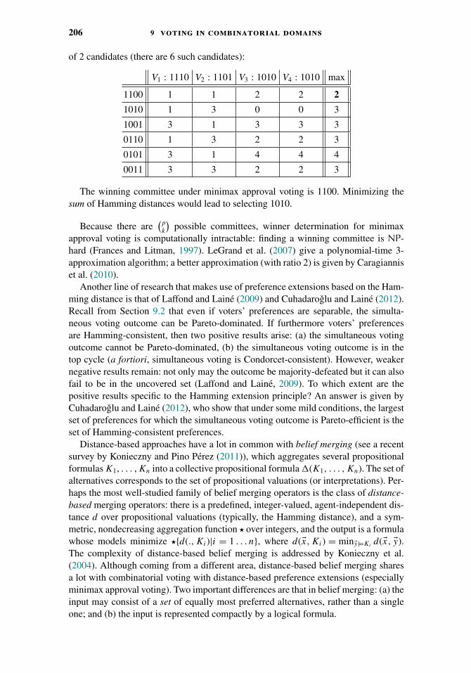
206 9 voting in combinatorial domains
of 2 candidates (there are 6 such candidates):
V1 : 1110 V2 : 1101 V3 : 1010 V4 : 1010 max
1100 1 1 2 2 2
1010 1 3 0 0 3
1001 3 1 3 3 3
0110 1 3 2 2 3
0101 3 1 4 4 4
0011 3 3 2 2 3
The winning committee under minimax approval voting is 1100. Minimizing thesum of Hamming distances would lead to selecting 1010.
Because there are(pk
)possible committees, winner determination for minimax
approval voting is computationally intractable: finding a winning committee is NP-hard (Frances and Litman, 1997). LeGrand et al. (2007) give a polynomial-time 3-approximation algorithm; a better approximation (with ratio 2) is given by Caragianniset al. (2010).
Another line of research that makes use of preference extensions based on the Ham-ming distance is that of Laffond and Laine (2009) and Cuhadaroglu and Laine (2012).Recall from Section 9.2 that even if voters’ preferences are separable, the simulta-neous voting outcome can be Pareto-dominated. If furthermore voters’ preferencesare Hamming-consistent, then two positive results arise: (a) the simultaneous votingoutcome cannot be Pareto-dominated, (b) the simultaneous voting outcome is in thetop cycle (a fortiori, simultaneous voting is Condorcet-consistent). However, weakernegative results remain: not only may the outcome be majority-defeated but it can alsofail to be in the uncovered set (Laffond and Laine, 2009). To which extent are thepositive results specific to the Hamming extension principle? An answer is given byCuhadaroglu and Laine (2012), who show that under some mild conditions, the largestset of preferences for which the simultaneous voting outcome is Pareto-efficient is theset of Hamming-consistent preferences.
Distance-based approaches have a lot in common with belief merging (see a recentsurvey by Konieczny and Pino Perez (2011)), which aggregates several propositionalformulas K1, . . . , Kn into a collective propositional formula �(K1, . . . , Kn). The set ofalternatives corresponds to the set of propositional valuations (or interpretations). Per-haps the most well-studied family of belief merging operators is the class of distance-based merging operators: there is a predefined, integer-valued, agent-independent dis-tance d over propositional valuations (typically, the Hamming distance), and a sym-metric, nondecreasing aggregation function � over integers, and the output is a formulawhose models minimize �{d(., Ki)|i = 1 . . . n}, where d( x, Ki) = min y|=Ki
d( x, y).The complexity of distance-based belief merging is addressed by Konieczny et al.(2004). Although coming from a different area, distance-based belief merging sharesa lot with combinatorial voting with distance-based preference extensions (especiallyminimax approval voting). Two important differences are that in belief merging: (a) theinput may consist of a set of equally most preferred alternatives, rather than a singleone; and (b) the input is represented compactly by a logical formula.
9 .3 approaches based on completion principles 207
9.3.2 Input Based on Rankings over Single Variables
In this section we focus specifically on the selection of a collective set of items S bya group of agents. The meaning we give here to “items” is extremely general and cancover a variety of situations, with two typical examples being committee elections,where the “items” are representatives, and group recommendations, where items areobjects such as books, movies, and so on.
Formally, this can be cast as a combinatorial domain where the set of binary issuesis X = {X1, . . . , Xp}, with Di = {0i , 1i} for each i. These binary issues correspondto a set of items C = {c1, . . . , cp}, where Xi = 1i (resp. 0i) means that item ci is(resp. is not) in the selection S. Because of the focus on the selection of a subsetof items, we change the notational convention by denoting an alternative x ∈ A ={01, 11} × . . . × {0p, 1p} as a subset of issues S composed of items cis with Xi = 1i .Thus, alternatives are elements of 2C .
In most cases, the set of feasible subsets is a proper subset of 2C , defined by aconstraint � restricting the set of feasible or allowed subsets. In committee elections,the most common constraints are cardinality constraints that restrict the size of acommittee, by specifying an exact size k, or a lower and/or an upper bound. Moregenerally, Lu and Boutilier (2011a) consider budget constraints, defined by a pricefor each item and a maximum total cost—hence the terminology budgeted socialchoice.
The approaches discussed in this section proceed by first eliciting from each agentsome preference information (typically, a ranking) over single items, then extend-ing these preferences over single items to preferences over sets of items, and finallyselecting a set of items S.
The most obvious way of doing so is multiwinner approval voting (which can,to some extent, be seen as the multiwinner version of simultaneous voting): eachvoter approves as many candidates as she wants, and the winners are the k candidatesapproved most often. In single nontransferable vote (SNTV) and bloc voting, thereis an additional restriction on the number of candidates approved: 1 in SNTV and k
in bloc voting (these rules are thus multiwinner versions of plurality and k-approval,respectively). Finally, in cumulative voting, voters distribute a fixed number of pointsamong the candidates, and the winners are the k candidates maximizing the numberof points. The common point of all these rules is that voters’ preferences are assumedto be separable; reformulated in terms of preference extensions, each input defines ascore over single candidates, and the total score of a candidate is the sum of the scoresit gets from the voters. Computational aspects of strategic behavior (manipulation bya single voter and control by the chair) for these multiwinner voting rules have beenstudied by Meir et al. (2008).
In the remainder of this section, we focus on classes of methods where the inputconsists of rankings over single items.
In committee elections, where the items are individuals supposed to represent thevoters, the rationale for the last step is that a committee election is used to elect anassembly whose members will make decisions on behalf of the society. As arguedby Betzler et al. (2013), finding a committee of representatives should satisfy twocriteria: representativity (the composition of the committee should globally reflectthe will of the voters), and accountability (each voter should be represented by a
208 9 voting in combinatorial domains
given member of the committee). In consensus recommendations, the rationale forthe last step is that each user will benefit from the best option according to her ownpreferences (Lu and Boutilier, 2011a); in this case, the “representative” of a voter isher most preferred item in S.6,7 The latter interpretation leads to an obvious choicefor defining representative items for voters: if the set of items S is chosen, then therepresentative item of voter i is c ∈ S if c �i c′ for all c′ ∈ C \ {c}. Alternatively, wesay that each agent is represented by an item in S. In committee elections, this principleis the basis of the Chamberlin and Courant multiwinner election scheme (discussedlater).
We now describe these multiwinner election schemes (grouped under the termi-nology “fully proportional representation”) more formally. For each voter i and eachitem c there is a misrepresentation value μi,c, representing the degree to which item c
misrepresents voter i. A positional misrepresentation function makes use of a scoringvector s = 〈s1, . . . , sp〉 such that s1 � . . . � sp. In particular, the Borda scoring vector sB is defined by sk = k for all k. By posi(c) we mean the position of item c in i’s
preference ranking (from 1 for the most preferred item to p for the least preferredone). The misrepresentation function induced by s is μi,c = sposi (c). Intuitively, si is theamount of dissatisfaction that a voter derives from being represented by an alternativethat she ranks in position i. Another simple way of defining a misrepresentation basedon approval ballots is: every voter submits a subset of candidates that she approves,and μi,c is 0 if i approves c, and 1 otherwise.
An assignment function π maps every voter to an item in the selected subset S.The misrepresentation of voter i under π is μi,π(i). Once individual misrepresentationhas been defined, we need to define the global misrepresentation of the society whenselecting a subset S of items. There are two traditional ways of doing so: utilitarianism(global misrepresentation is the sum of all individual misrepresentation) and egalitar-ianism (global misrepresentation is the misrepresentation of the least well-representedagent). Formally, the global misrepresentation of assignment π is defined as:
� (utilitarianism) μU (π ) = ∑i�n μi,π(i).
� (egalitarianism) μE(π ) = maxi�n μi,π(i).
Finally, let F be the set of feasible subsets of items; typically, if k items are to beelected then F is the set Sk of all subsets of C of size k.
The Chamberlin and Courant scheme (Chamberlin and Courant, 1983) simplyoutputs the committee of size k that minimizes μU . Because there is no constraint onthe assignment function, every voter is assigned to her preferred item in the selectedsubset S. That is, π(i) = arg minc∈S μi,c. Then, her misrepresentation when selectingthe feasible subset S is equal to μi,S = minc∈S μi,c. The best committee is then thefeasible subset S minimizing μU (π) (under utilitarianism) or S that minimizes μE(π)(under egalitarianism). The Monroe scheme (Monroe, 1995) additionally requires that
6 As discussed by Lu and Boutilier (2011a), this can also be seen as a segmentation problem (Kleinberg et al.,2004), where one more generally seeks k solutions to some combinatorial optimization problem that will beused by n � k different users, each with a different objective value on items; optimization requires segmentingusers into k groups depending on which of the k items gives them the greatest benefit.
7 Skowron et al. (2015) generalize this scheme by taking into account more than one item by agent, but still givingmore importance to an agent’s most preferred item than to her second best preferred item, etc.
9 .3 approaches based on completion principles 209
the assignment π is balanced: each candidate in S must be assigned to at least !n/k"voters.8 Formally, the Monroe scheme selects the allocation π minimizing μU (π)subject to the constraints |π−1(s)| � !n
k" for all s ∈ Range(π).
Budgeted social choice (Lu and Boutilier, 2011a) generalizes Chamberlin-Courantby redefining feasibility via a budget constraint: Each item c has a fixed cost (to becounted if x is selected) and a unit cost (to be counted k times if k agents are representedby the item), the maximum budget is K , and F is the set of all assignments with totalcost � K .
The egalitarian version of multiwinner schemes is due to Betzler et al. (2013). Elkindet al. (2014a) discuss some properties of multiwinner voting schemes.
Example 9.6. Let C = {c1, c1, c3, c4}, K = 2, and the following 4 agents’preferences:
〈 c1 � c2 � c3 � c4,
c1 � c2 � c3 � c4,
c1 � c3 � c2 � c4,
c1 � c3 � c2 � c4,
c2 � c4 � c3 � c1,
c4 � c3 � c2 � c1 〉.For the Borda misrepresentation function, the optimal Chamberlin-Courant committeeof 2 items is {c1, c4}, whereas for Monroe it is {c1, c2}. For the egalitarian versions,both {c1, c4} and {c2, c3} are optimal for Chamberlin-Courant and {c2, c3} is optimalfor Monroe.
Because the set of feasible subsets is generally exponentially large, finding the opti-mal subset is highly nontrivial. Brams and Potthoff (1998) were the first to discuss thecomputation of the Chamberlin-Courant and the Monroe voting schemes, showing thatthe optimal committee can be determined using integer programming. This providesa method that works in practice when the number of voters and items are small, butmay not scale up well. They formulate an improved integer program for settings wherethe number of agents is large, but this modified integer program is still too large to besolved when the number of items is large.
One cannot really do better in the general case; indeed, we have the followinghardness results:
� Winner determination for the Chamberlin-Courant and the Monroe schemes withapproval ballots are both NP-complete (Procaccia et al., 2008)
� Winner determination for the Chamberlin-Courant scheme with the Borda misrepresen-tation function is NP-complete (Lu and Boutilier, 2011a)
� Winner determination for the minimax versions of the Chamberlin-Courant and Monroeschemes is NP-complete (Betzler et al., 2013)
8 In indirect democracy, that is, when the set of representatives has to make a decision on behalf of the society, itmay be a good idea to give more power to people who represent more people than to those who represent lesspeople; for instance, Chamberlin and Courant suggested to give to each committee member a weight equal tothe number of voters she represents.
210 9 voting in combinatorial domains
Some slightly more positive results are obtained:
� Parameterized complexity. Procaccia et al. (2008) show that winner determination forChamberlin-Courant and Monroe is tractable for small committees: if the size of thesubset to be selected is constant, then winner determination is polynomial for both votingschemes. Betzler et al. (2013) investigate further the parameterized complexity of fullyproportional representation by establishing a mixture of positive and negative results:they mainly prove fixed-parameter tractability with respect to the number of candidatesor the number of voters, but fixed-parameter intractability with respect to the number ofwinners.
� Approximation: Lu and Boutilier (2011a) give a polynomial algorithm with approxi-mation ratio 1 − 1
efor Chamberlin-Courant with the Borda misrepresentation function.
Skowron et al. (2013a,c) give further approximability results.� Domain restrictions: for single-peaked profiles, most multiwinner problems discussed
above become polynomial; the only rule that remains NP-hard for single-peaked elec-torates is the classical Monroe rule (Betzler et al., 2013). These results are extendedby Cornaz et al. (2012) to profiles with bounded single-peaked width, and by Yu et al.(2013) who consider profiles that are more generally single-peaked on a tree. Skowronet al. (2013b) address the case of single-crossing profiles.
Finally, the generalization of full proportional representation schemes to incompletepreferences was considered by Lu and Boutilier (2013) (see also Chapter 10).
The notion of Condorcet winning set (Elkind et al., 2015a) also evaluates a subsetaccording to a best item in it. The criteria for selecting a “best” subset does not usea misrepresentation function but is simply based on the Condorcet principle: S ⊆ C
is a Condorcet winning set if for every z /∈ S, a majority of voters prefers some s ∈ S
to z. For every m-candidate profile, there is a Condorcet winning set of size at mostlog2 m + 1, therefore, finding a Condorcet winning set can be done by enumeratingall subsets of candidates of size !log2 m" + 1, i.e., in quasipolynomial time. It mayactually be even easier: it is an open issue whether for all k there exists a profile forwhich the smallest Condorcet winning set has size k.
9.3.3 Hypercube-Based Inputs
Specifying top-based inputs (respectively, rankings over variables) needs O(np)(respectively, O(np log p)) space, hence the communication requirement of the twoprevious subclasses of methods is low: each agent needs only to report O(np) (respec-tively, O(np log p)) bits to the central authority. On the other hand, their applicabilityis very weak, because only a tiny fraction of preference relations comply with therequired domain restrictions. We now consider more expressive approaches that arebased on compact representations: the votes, or a significant part of the votes, are notgiven extensively but are described in some formal language that comes with a func-tion mapping any input of the language to a (partial or complete) vote (Lang, 2004).Formally, a compact preference representation language is a pair L = 〈�L, IL〉 where�L is a formal language, and IL is a function from �L to the set of preference relationsover A. IL(�L) is the set of all preference relations expressible in L. A language L1 ismore expressive than L2 if IL1 (�L1 ) ⊃ IL2 (�L2 ) and more succinct than L2 if there is a
9 .3 approaches based on completion principles 211
function f : �L2 → �L1 and a polynomial function pol such that for all σ ∈ �L2 , wehave (i) |f (σ )| � pol(|σ |) and (ii) IL1 (f (σ )) = IL2 (σ ). Conditions (i) and (ii) togethermean that any preference relation expressible in L2 can also be expressed in L1 withouta superpolynomial increase in the size of expression.
If a language L is totally expressive (i.e., IL(�L) is the set of all rankings over D)then the worst-case size necessary for expressing a ranking is exponentially large in thenumber of variables.9 Therefore, there is a trade-off to be made between having a fullyexpressive language which, at least for some preference relations, will not be compactat all, or making a domain restriction that will allow for a compact input in all cases.
Some of the solutions advocated in the previous sections were, to some extent,making use of very rough compact preference representation languages. Expressingonly the top alternative, say 111, is a compact representation of the partial preferencerelation
111 � A \ {111}or, in the case of the Hamming distance completion, of the complete preorder
111 �110101001
�100010001
� 000.
Expressing a ranking over single items is a compact representation of a partial orcomplete preorder over committees: for 2-committees and the Chamberlin-Courantscheme, for instance, 1 � 2 � 3 � 4 is a compact representation of
{1, 4}{1, 2}{1, 3}
� {2, 3}{2, 4} � {3, 4}.
As already discussed, these first two compact representation languages are admit-tedly very compact, but also very inexpressive. We now give some examples of moreexpressive languages.
The first compact representation language we consider is that of conditional pref-erence networks (CP-nets). CP-nets (Boutilier et al., 2004) allow for a compact rep-resentation of the preference hypercube associated with a preference relation over D.Given a preference relation � over D = ∏n
i=1{0i , 1i}, the preference hypercube �H
is the restriction of � to the set of pairs of alternatives x, y differing on only onevariable (such as, for instance, 0101 and 0111). CP-nets are based on the notion of con-ditional preferential independence (Keeney and Raiffa, 1976): given a strict preferencerelation �, Xi ∈ X , Y ⊆ X \ {Xi} and Z = X \ ({Xi} ∪ Y ), we say that Xi is preferen-tially independent of Y given Z with respect to � if for any xi, x
′i ∈ Di , y, y ′ ∈ DY , and
z ∈ DZ , we have (xi, y, z) � (x ′i , y, z) if and only if (xi, y ′, z) � (x ′
i , y ′, z). A CP-netN over A consists of two components.
9 A simple proof of this fact in the case of binary variables: for p variables there are (2p)! possible rankings, andthe best we can do to express a ranking is to use log((2p)!) bits in the worst case; and log((2p)!) is exponentialin p.
212 9 voting in combinatorial domains
� The first component is a directed graph G expressing preferential independence relationsbetween variables: if ParG(Xi) denotes the set of the parents of Xi in G, then everyvariable Xi is preferentially independent of X \ (Par(Xi) ∪ {Xi}) given Par(Xi).
� The second component is, for each variable Xi , a set of linear orders �i u over Di , called
conditional preferences, for each u ∈ DParG(Xi ). These conditional preferences form theconditional preference table for issue Xi , denoted by CPT (Xi).
The preference relation �N induced by N is the transitive closure of
{(ai, u, z) � (bi, u, z) | i � p; u ∈ DParG(Xi ); ai, bi ∈ Di, ai �i u bi
z ∈ D−(ParG(Xi )∪{Xi })}.When all issues are binary, �N is equivalent to a preference hypercube and N is acompact representation of this preference hypercube, whose size is the cumulative sizeof all its conditional preference tables.
Example 9.7. Let p = 3. The following represents a CP-net N together with itsinduced preference hypercube �N . For the sake of simplicity, 000 represents thealternative 010203, and so on.
X1 X2 X3
01 1101 : 02 12
11 : 12 02
02 : 03 13
12 : 13 03
000 001
010 011
100 101
110 111
Group decision making in multi-issue domains via CP-net aggregation has beenconsidered in a number of papers, which we briefly review in a nonchronologicalorder. We will discuss in Section 9.4 the role of CP-nets in sequential voting (Lang andXia, 2009; Airiau et al., 2011): this way of proceeding sequentially leads to interleaveelicitation and aggregation, and elicits only a small part of the voters’ CP-nets. Anotherway of proceeding consists in first eliciting the voters’ CP-nets entirely, then proceedingto aggregation. Then, two ways are possible.
The first aggregation consists of mapping each of the individual CP-nets to its asso-ciated preference relation, and aggregating these into a collective preference relation.This method was initiated by Rossi et al. (2004), who consider several such aggregationfunctions, and was studied further by Li et al. (2010), who give algorithms for com-puting Pareto-optimal alternatives with respect to the preference relations induced bythe CP-nets, and fair alternatives with respect to a cardinalization of these preferencerelations.
A second technique, considered by Xia et al. (2008), Li et al. (2011), and Conitzeret al. (2011b), consists of aggregating the individual CP-nets into a collective CP-net, and then outputting the nondominated alternatives of this collective CP-net. Nodomain restriction is made on the individual CP-nets. For every set of “neighboring”alternatives (differing only in the value of one issue), a local voting rule (typically
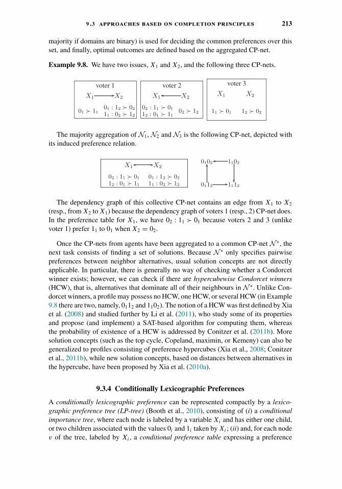
9 .3 approaches based on completion principles 213
majority if domains are binary) is used for deciding the common preferences over thisset, and finally, optimal outcomes are defined based on the aggregated CP-net.
Example 9.8. We have two issues, X1 and X2, and the following three CP-nets.
voter 1
X1 X2
01 1101 : 12 02
11 : 02 12
voter 2
X1 X2
02 : 11 01
12 : 01 1102 12
voter 3
X1 X2
11 01 12 02
The majority aggregation of N1, N2 and N3 is the following CP-net, depicted withits induced preference relation.
X1 X2
02 : 11 01
12 : 01 11
01 : 12 02
11 : 02 12
0102
0112
1102
1112
The dependency graph of this collective CP-net contains an edge from X1 to X2
(resp., from X2 to X1) because the dependency graph of voters 1 (resp., 2) CP-net does.In the preference table for X1, we have 02 : 11 � 01 because voters 2 and 3 (unlikevoter 1) prefer 11 to 01 when X2 = 02.
Once the CP-nets from agents have been aggregated to a common CP-net N ∗, thenext task consists of finding a set of solutions. Because N ∗ only specifies pairwisepreferences between neighbor alternatives, usual solution concepts are not directlyapplicable. In particular, there is generally no way of checking whether a Condorcetwinner exists; however, we can check if there are hypercubewise Condorcet winners(HCW), that is, alternatives that dominate all of their neighbours in N ∗. Unlike Con-dorcet winners, a profile may possess no HCW, one HCW, or several HCW (in Example9.8 there are two, namely, 0112 and 1102). The notion of a HCW was first defined by Xiaet al. (2008) and studied further by Li et al. (2011), who study some of its propertiesand propose (and implement) a SAT-based algorithm for computing them, whereasthe probability of existence of a HCW is addressed by Conitzer et al. (2011b). Moresolution concepts (such as the top cycle, Copeland, maximin, or Kemeny) can also begeneralized to profiles consisting of preference hypercubes (Xia et al., 2008; Conitzeret al., 2011b), while new solution concepts, based on distances between alternatives inthe hypercube, have been proposed by Xia et al. (2010a).
9.3.4 Conditionally Lexicographic Preferences
A conditionally lexicographic preference can be represented compactly by a lexico-graphic preference tree (LP-tree) (Booth et al., 2010), consisting of (i) a conditionalimportance tree, where each node is labeled by a variable Xi and has either one child,or two children associated with the values 0i and 1i taken by Xi ; (ii) and, for each nodev of the tree, labeled by Xi , a conditional preference table expressing a preference
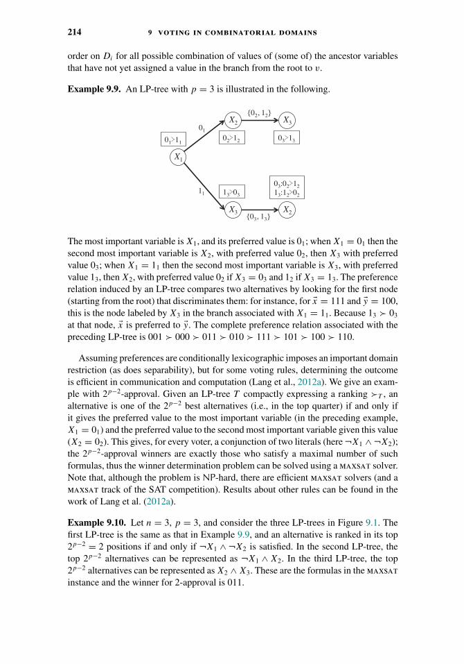
214 9 voting in combinatorial domains
order on Di for all possible combination of values of (some of) the ancestor variablesthat have not yet assigned a value in the branch from the root to v.
Example 9.9. An LP-tree with p = 3 is illustrated in the following.
The most important variable is X1, and its preferred value is 01; when X1 = 01 then thesecond most important variable is X2, with preferred value 02, then X3 with preferredvalue 03; when X1 = 11 then the second most important variable is X3, with preferredvalue 13, then X2, with preferred value 02 if X3 = 03 and 12 if X3 = 13. The preferencerelation induced by an LP-tree compares two alternatives by looking for the first node(starting from the root) that discriminates them: for instance, for x = 111 and y = 100,this is the node labeled by X3 in the branch associated with X1 = 11. Because 13 � 03
at that node, x is preferred to y. The complete preference relation associated with thepreceding LP-tree is 001 � 000 � 011 � 010 � 111 � 101 � 100 � 110.
Assuming preferences are conditionally lexicographic imposes an important domainrestriction (as does separability), but for some voting rules, determining the outcomeis efficient in communication and computation (Lang et al., 2012a). We give an exam-ple with 2p−2-approval. Given an LP-tree T compactly expressing a ranking �T , analternative is one of the 2p−2 best alternatives (i.e., in the top quarter) if and only ifit gives the preferred value to the most important variable (in the preceding example,X1 = 01) and the preferred value to the second most important variable given this value(X2 = 02). This gives, for every voter, a conjunction of two literals (here ¬X1 ∧ ¬X2);the 2p−2-approval winners are exactly those who satisfy a maximal number of suchformulas, thus the winner determination problem can be solved using a maxsat solver.Note that, although the problem is NP-hard, there are efficient maxsat solvers (and amaxsat track of the SAT competition). Results about other rules can be found in thework of Lang et al. (2012a).
Example 9.10. Let n = 3, p = 3, and consider the three LP-trees in Figure 9.1. Thefirst LP-tree is the same as that in Example 9.9, and an alternative is ranked in its top2p−2 = 2 positions if and only if ¬X1 ∧ ¬X2 is satisfied. In the second LP-tree, thetop 2p−2 alternatives can be represented as ¬X1 ∧ X2. In the third LP-tree, the top2p−2 alternatives can be represented as X2 ∧ X3. These are the formulas in the maxsatinstance and the winner for 2-approval is 011.
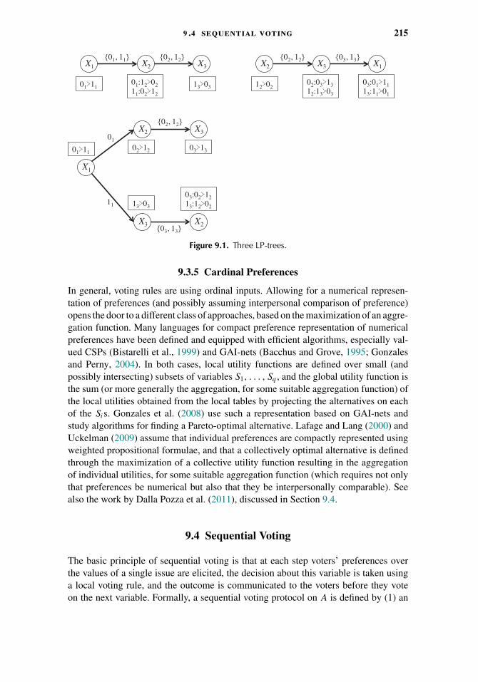
9 .4 sequential voting 215
Figure 9.1. Three LP-trees.
9.3.5 Cardinal Preferences
In general, voting rules are using ordinal inputs. Allowing for a numerical represen-tation of preferences (and possibly assuming interpersonal comparison of preference)opens the door to a different class of approaches, based on the maximization of an aggre-gation function. Many languages for compact preference representation of numericalpreferences have been defined and equipped with efficient algorithms, especially val-ued CSPs (Bistarelli et al., 1999) and GAI-nets (Bacchus and Grove, 1995; Gonzalesand Perny, 2004). In both cases, local utility functions are defined over small (andpossibly intersecting) subsets of variables S1, . . . , Sq , and the global utility function isthe sum (or more generally the aggregation, for some suitable aggregation function) ofthe local utilities obtained from the local tables by projecting the alternatives on eachof the Sis. Gonzales et al. (2008) use such a representation based on GAI-nets andstudy algorithms for finding a Pareto-optimal alternative. Lafage and Lang (2000) andUckelman (2009) assume that individual preferences are compactly represented usingweighted propositional formulae, and that a collectively optimal alternative is definedthrough the maximization of a collective utility function resulting in the aggregationof individual utilities, for some suitable aggregation function (which requires not onlythat preferences be numerical but also that they be interpersonally comparable). Seealso the work by Dalla Pozza et al. (2011), discussed in Section 9.4.
9.4 Sequential Voting
The basic principle of sequential voting is that at each step voters’ preferences overthe values of a single issue are elicited, the decision about this variable is taken usinga local voting rule, and the outcome is communicated to the voters before they voteon the next variable. Formally, a sequential voting protocol on A is defined by (1) an
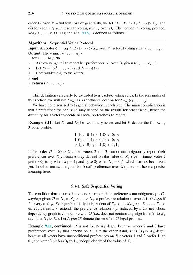
216 9 voting in combinatorial domains
order O over X – without loss of generality, we let O = X1 � X2 � · · ·� Xp; and(2) for each i � p, a resolute voting rule ri over Di . The sequential voting protocolSeqO(r1, . . . , rp) (Lang and Xia, 2009) is defined as follows.
Algorithm 1 Sequential Voting ProtocolInput: An order O = X1 � X2 � · · ·� Xp over X ; p local voting rules r1, . . . , rp.Output: The winner (d1, . . . , dp)1 for t = 1 to p do2 Ask every agent i to report her preferences �i
t over Dt given (d1, . . . , dt−1).3 Let Pt = 〈�1
t , . . . ,�nt 〉 and dt = rt (Pt ).
4 Communicate dt to the voters.5 end6 return (d1, . . . , dp)
This definition can easily be extended to irresolute voting rules. In the remainder ofthis section, we will use SeqO as a shorthand notation for SeqO(r1, . . . , rp).
We have not discussed yet agents’ behavior in each step. The main complication isthat a preference for one issue may depend on the results for other issues, hence thedifficulty for a voter to decide her local preferences to report.
Example 9.11. Let X1 and X2 be two binary issues and let P denote the following3-voter profile:
1112 � 0112 � 1102 � 0102
1102 � 1112 � 0112 � 0102
0112 � 0102 � 1102 � 1112
If the order O is X2 � X1, then voters 2 and 3 cannot unambiguously report theirpreferences over X2, because they depend on the value of X1 (for instance, voter 2prefers 02 to 12 when X1 = 11 and 12 to 02 when X1 = 01), which has not been fixedyet. In other terms, marginal (or local) preference over X2 does not have a precisemeaning here.
9.4.1 Safe Sequential Voting
The condition that ensures that voters can report their preferences unambiguously is O-legality: given O = X1 � X2 � · · ·� Xp, a preference relation � over A is O-legal iffor every k � p, Xk is preferentially independent of Xk+1, . . . Xp given X1, . . . , Xk−1;or, equivalently, � extends the preference relation �N induced by a CP-net whosedependency graph is compatible with O (i.e., does not contain any edge from Xi to Xj
such that Xj � Xi). Let Legal(O) denote the set of all O-legal profiles.
Example 9.11, continued. P is not (X2 � X1)-legal, because voters 2 and 3 havepreferences over X2 that depend on X1. On the other hand, P is (X1 � X2)-legal,because all voters have unconditional preferences on X1: voters 1 and 2 prefer 11 to01, and voter 3 prefers 01 to 11, independently of the value of X2.

9 .4 sequential voting 217
In presence of the O-legality domain restriction, we say that sequential voting is safe.In this section we assume O to be fixed and apply sequential voting to the domain ofO-legal profiles only. A crucial property of simultaneous voting under the separabilityrestriction carries over to safe sequential voting: it makes sense for a voter to report herlocal preferences on the current issue given the value of earlier issues, without havingto wonder about the values of issues that have not been decided yet.
When all agents’ preferences are O-legal, a sequential voting protocol can also beconsidered as a voting rule, because a voter’s preference on the values of Xi given thevalues of earlier variables is unambiguously defined given her preference relation overA. More precisely, given any O-legal profile P , SeqO(P ) is defined to be the output ofthe sequential voting protocol where in step 2, Pt = 〈�1
t , . . . ,�nt 〉 where �i
t representslocal preferences of agent i over Dt given X1 = d1, . . . , Xt−1 = dt−1.
Example 9.12. Suppose there are two binary issues X1 and X2. Let P denote thesame profile as in Example 9.11. Let O = X1 � X2. As we discussed, P is O-legal.To apply SeqO(maj, maj), where maj denote the majority rule, in step 1 the votersare asked to report their (unconditional) preferences on X1, which gives P1 = 〈11 �01, 11 � 01, 01 � 11〉. Therefore, d1 = maj(P1) = 11. In step 2, the voters report theirpreferences over D2 given X1 = 11, which leads to P2 = 〈12 � 02, 02 � 12, 02 � 12〉,and then d2 = maj(P2) = 02. Therefore, SeqO(maj, maj)(P ) = 1102.
Normative Properties
We recall from Chapter 2 that one classical way to assess voting rules is to studywhether they satisfy certain normative properties. In this subsection we examine thenormative properties of safe sequential voting.
Classical normative properties are defined for voting rules where the input is com-posed of linear orders over the alternatives. We note that SeqO(P ) is only definedfor O-legal profiles. Some normative properties can be easily extended to SeqO(P ),for example anonymity and consistency, while others need to be modified. For exam-ple, the classical neutrality axiom states that for any profile P and any permutationM of the alternatives, r(M(P )) = M(r(P )). However, even if P is O-legal, M(P )might not be O-legal. Therefore, we will focus on a weaker version of neutrality thatrequires r(M(P )) = M(r(P )) for all P and M such that both P and M(P ) are O-legal.Monotonicity can be modified in a similar way.
Whether SeqO satisfies a specific normative property often depends on whether thelocal voting rules satisfy the same property. Some properties are inherited by sequentialcompositions from their local rules ri ; for others, satisfaction of the property by thelocal voting rules is merely a necessary but not sufficient condition.
Theorem 9.13 (Lang and Xia, 2009).
� SeqO(r1, . . . , rp) satisfies anonymity (respectively, consistency) if and only if ri satisfiesanonymity (consistency) for all i = 1, . . . , p;
218 9 voting in combinatorial domains
� if SeqO(r1, . . . , rp) satisfies neutrality (respectively, Condorcet-consistency, partici-pation, and Pareto-efficiency) then ri satisfies neutrality (respectively, Condorcet-consistency, participation, and Pareto-efficiency) for all i = 1, . . . , p;
� SeqO(r1, . . . , rp) satisfies monotonicity if and only if rp satisfies monotonicity.
Proofs for the normative properties mentioned in Theorem 9.13 follow a similarpattern. Take consistency, for example. Recall that a voting rule r satisfies consistency iffor all disjoint profiles P1 and P2 such that r(P1) = r(P2), we have r(P1 ∪ P2) = r(P1)(see Chapter 1). We first prove that consistency can be lifted from all local rules totheir sequential composition SeqO(r1, . . . , rp). For any disjoint sets of profiles P1 andP2 such that SeqO(r1, . . . , rp)(P1) = SeqO(r1, . . . , rp)(P2), let d denote the outcome.We then prove that SeqO(r1, . . . , rp)(P1 ∪ P2) = d = (d1, . . . , dp) by induction on theround t of sequential voting. When t = 1, let P 1
1 and P 12 denote the agents’ preferences
over X1, which are well-defined because P1 and P2 are O-legal. Due to consistencyof r1, we have r1(P 1
1 ∪ P 12 ) = d1. Suppose the outcome of sequential voting is the
same as in d up to round k − 1. It is not hard to verify that in round k, the winner isdk by considering agents’ preferences over Xt conditioned on previous issues takingd1, . . . , dk−1. This proves that SeqO(r1, . . . , rp) satisfies consistency.
Conversely, if SeqO(r1, . . . , rp) satisfies consistency and for the sake of contradic-tion suppose that a local rule does not satisfy consistency. Let t denote the smallestnumber such that rt is not consistent, and let P t
1 , Pt2 denote the profiles over Xt with
rt (P t1 ) = rt (P t
2 ) �= rt (P t1 ∪ P t
2 ). Let r1, . . . , rt−1, rt+1, . . . , rp be rules that always out-put the same winner regardless of the local profile. We can extend P t
1 and P t2 to
profiles P1, P2 over the whole combinatorial domain so that SeqO(r1, . . . , rp)(P1) =SeqO(r1, . . . , rp)(P2), and agents’ local preferences over Xt are P t
1 and P t2 . It is not
hard to verify that SeqO(r1, . . . , rp)(P1) �= SeqO(r1, . . . , rp)(P1 ∪ P2), which contra-dicts the assumption that SeqO(r1, . . . , rp) satisfies consistency.
In fact, for neutrality and Pareto-efficiency, a stronger result has been proved forirresolute sequential voting rules: Xia and Lang (2009) show that except in the casewhere the domain is composed of two binary issues, the only neutral irresolute sequen-tial voting rules are dictatorships, antidictatorships,10 and the trivial irresolute rule thatalways outputs the whole set of alternatives; and the only Pareto-efficient irresolutesequential voting rules are dictatorships and the trivial irresolute rule. When the domainis composed of two binary issues, sequential majority is neutral and Pareto-efficient.
Strategic Behavior
In the previous subsection, when we talked about normative properties, it was implicitlyassumed that agents were truthful. However, in practice an agent may misreport herpreferences at step 2 of the sequential voting protocol (Algorithm 1). If some variablesare nonbinary, then sequential voting will inherit manipulability from the local rules,even if the profile is separable. However, in case all variables are binary, it is not imme-diately clear if a sequential voting rule defined over O-legal profiles is strategyproof
10 A rule is an antidictatorship if there exists an agent such that the winner is always her least preferred alternative.
9 .4 sequential voting 219
(see Chapters 2 and 6), since the Gibbard-Satterthwaite Theorem is not directly appli-cable. The following example shows that sequential voting is not strategyproof, evenwhen all variables are binary, and the agents’ preferences are O-legal for some O.
Example 9.14. Let P be the profile defined in Example 9.11. If agent 1 knows thepreferences of agent 2 and agent 3, then she has no incentive to vote truthfully on issueX1, even though her preference relation is separable: if she votes for 1 sincerely, thenthe outcome is 10. If she votes for 0 instead, then the outcome is 01, which is better toher.
The problem of characterizing strategyproof voting rules in binary multi-issuedomains has received some attention. Barbera et al. (1991) characterize strategyproofvoting rules when the voters’ preferences are separable, and each issue is binary. Ju(2003) characterizes all strategyproof voting rules on binary multi-issue domains (sat-isfying a mild additional condition) where each issue can take three values: “good,”“bad,” and “null.” Le Breton and Sen (1999) prove that if the voters’ preferencesare separable, and the restricted preference domain of the voters satisfies a rich-ness condition, then a voting rule is strategyproof if and only if it is a simultane-ous voting rule for which each local voting rule is strategyproof over its respectivedomain.
We may wonder whether this extends to safe sequential voting. However, the follow-ing impossibility theorem of Xia and Conitzer (2010a) answers the question negatively:there is no strategyproof sequential voting rule on Legal(O)n that satisfies nonimposi-tion, except a dictatorship. Xia and Conitzer (2010a) also prove a positive result in thefurther restricted case of O-legal conditionally lexicographic preferences: essentially,the strategyproof rules on this domain are generalized sequential voting rules, wherethe choice of the local rule to apply on a given issue may depend on the values takenby more important issues.
9.4.2 Sequential Voting: The General Case
In the absence of O-legality, sequential voting suffers from the same problem assimultaneous voting in the absence of separability: there is no clear way for voters toreport their local preferences on the domain of an issue, since it may depend on thevalue of issues yet to be decided. Moreover, choosing the agenda (the order on whichthe issues are decided) can be tricky: What is a good agenda? Who chooses it? Thisproblem is raised by Airiau et al. (2011), who suggest designing a voting procedurefor choosing the agenda: each voter reports its dependency graph and these graphsare aggregated into an acyclic graph, for instance using a distance-based aggregationfunction. Another approach to unrestricted sequential voting is described by DallaPozza et al. (2011), who assume that at each stage, voters report their local preferencesaccording to the projection of a weighted CSP on the current variable.
Another challenge in the analysis of sequential voting without the O-legalityassumption is that the outcome may depend on the order in which the issues aredecided. This can give the chair (or whoever chooses the order) an effective way ofcontrolling the election (see Chapter 7). This can be seen in the following example:

220 9 voting in combinatorial domains
Example 9.3, continued. Suppose the voters report their preferences optimistically,which is known to the chair. If S is decided before T , then we get k + 1 votes for 1S ,k votes for 0S , leading to the local outcome 1S ; then, given S = 1S , we have 2k votesfor 0T and 1 vote for 1T , therefore the final outcome is 1S0T . Symmetrically, if T isdecided before S, the final outcome is 0S1T . Therefore, the chair’s strategy can be tochoose the order S � T if she prefers 1S0T to 0S1T , and the order T � S otherwise.(Note that 1S1T and 0S0T cannot be obtained).
This shows that the chair can sometimes, and to some extent, control the election byfixing the agenda (see also Chapter 7). This drawback of sequential voting is howevertempered by the fact that under some reasonable assumptions about the way the voters’sbehaviors are represented, in most cases, most of these agenda control problems areNP-hard (Conitzer et al., 2009a).
We mentioned above that in the absence ofO-legality, there is no clear way for votersto report their local preferences on the domain of a variable. However, there is a casewhere voters may in fact be able to determine valid reports of their local preferences.When voters’ preferences are assumed to be common knowledge, the sequential votingprotocol can be framed as an extensive-form game, called a strategic sequential votingprocess, denoted by SSVO (Xia et al., 2011a). We assume that all variables are binary.Without loss of generality, let O = X1 � · · ·� Xp. The game is defined as follows:
� The players are the voters; their preferences are linear orders over A; their possibleactions at stage t � p are 0t and 1t .
� In each stage t , all voters vote on Xt simultaneously, rt is used to choose the winningvalue dt for Xt , and dt is reported back to the voters.
� We assume complete information: all voters know the other voters’ preferences, thelocal voting rules r1, . . . , rp and the order O.
When all issues are binary, SSVO can be solved by backward induction where in eachstage all voters move simultaneously and perform a dominant strategy, as illustrated inthe following example.
Example 9.15. Let P be the profile defined in Example 9.11. If the outcome of thefirst stage of sequential voting is 11, then in the second stage it is voter 1’s dominantstrategy to vote for 12 because 1112 �1 1202 and the majority rule is strategyproof.Similarly, in this case voters 2 and 3 will vote for 02. Therefore, by the majority rule,the winner will be 1102. Similarly, if the outcome of the first stage of sequential votingis 01, then the votes at the second stage will be unanimously 02, and the winner willbe 0112. Given this reasoning, in the first stage, each agent is comparing 1102 to 0112,and will vote 11 if he prefers 1102 to 0112 and 01 if he prefers 0112 to 1102. Again wehave two alternatives, and the majority rule is strategyproof. This means that voter 1will vote for 01, voter 2 will vote for 11, and voter 3 will vote for 01. Hence, the winnerfor X1 is 01, and the overall winner is 0112. This backward induction process is shownin Figure 9.2.
In Example 9.15, the backward induction winner is unique. This observation can beextended to an arbitrary number of binary issues. Let SSVO(P ) denote the backward
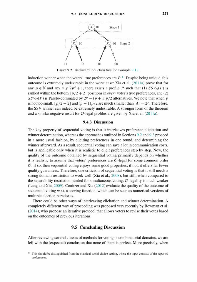
9 .5 concluding discussion 221
Figure 9.2. Backward induction tree for Example 9.15.
induction winner when the voters’ true preferences are P .11 Despite being unique, thisoutcome is extremely undesirable in the worst case: Xia et al. (2011a) prove that forany p ∈ N and any n � 2p2 + 1, there exists a profile P such that (1) SSVO(P ) isranked within the bottom !p/2 + 2" positions in every voter’s true preferences, and (2)SSVO(P ) is Pareto-dominated by 2p − (p + 1)p/2 alternatives. We note that when p
is not too small, !p/2 + 2" and (p + 1)p/2 are much smaller than |A| = 2p. Therefore,the SSV winner can indeed be extremely undesirable. A stronger form of the theoremand a similar negative result for O-legal profiles are given by Xia et al. (2011a).
9.4.3 Discussion
The key property of sequential voting is that it interleaves preference elicitation andwinner determination, whereas the approaches outlined in Sections 9.2 and 9.3 proceedin a more usual fashion, by eliciting preferences in one round, and determining thewinner afterward. As a result, sequential voting can save a lot in communication costs,but is applicable only when it is realistic to elicit preferences step by step. Now, thequality of the outcome obtained by sequential voting primarily depends on whetherit is realistic to assume that voters’ preferences are O-legal for some common orderO: if so, then sequential voting enjoys some good properties; if not, it offers far fewerquality guarantees. Therefore, one criticism of sequential voting is that it still needs astrong domain restriction to work well (Xia et al., 2008); but still, when compared tothe separability restriction needed for simultaneous voting, O-legality is much weaker(Lang and Xia, 2009). Conitzer and Xia (2012) evaluate the quality of the outcome ofsequential voting w.r.t. a scoring function, which can be seen as numerical versions ofmultiple election paradoxes.
There could be other ways of interleaving elicitation and winner determination. Acompletely different way of proceeding was proposed very recently by Bowman et al.(2014), who propose an iterative protocol that allows voters to revise their votes basedon the outcomes of previous iterations.
9.5 Concluding Discussion
After reviewing several classes of methods for voting in combinatorial domains, we areleft with the (expected) conclusion that none of them is perfect. More precisely, when
11 This should be distinguished from the classical social choice setting, where the input consists of the reportedpreferences.
222 9 voting in combinatorial domains
choosing a method, we have to make a trade-off between generality, communication(and, to a lesser extent, computation) costs, and the quality of the outcome, evaluatedwith respect to classical social choice criteria. If specific domain restrictions suchas separability or, more generally, O-legality, are realistic for the case at hand, thenmany of the methods discussed in this chapter work reasonably well. Otherwise, onehas to be prepared to make some trade-off between communication requirements andthe quality of the outcome. One possibility that has not really been developed yetis to choose some intermediate method that requires some weak domain restriction,some reasonable communication and computation costs, and offers some reasonableguarantees about the quality of the outcome.
Voting in combinatorial domains is related to several other issues studied in thisbook and elsewhere:
� Incomplete information and communication (Chapter 10): as some communication sav-ing can be made by eliciting only a part of the voters’ preferences, winner determinationin combinatorial domains can benefit from approaches to winner determination fromincomplete preferences as well as from the design of communication-efficient votingprotocols.
� Judgment aggregation (Chapter 17) is also concerned with making common decisionsabout possibly interrelated issues. There are interesting parallels between judgmentaggregation and voting in combinatorial domains. Simultaneous voting corresponds tosome extent to proposition-wise voting: while the first works well when preferences areseparable, the second outputs a consistent outcome if the agenda enjoys an independenceproperty that resembles separability. Note that in judgment aggregation, difficulties areoften caused by the logical relations between the elements of the agenda, while in votingin combinatorial domains, they are mainly due to preferential dependencies. Relatingboth areas is a promising research direction; see Grandi and Endriss (2011) for somefirst steps in this direction.
� Fair division of indivisible items (Chapter 12) is another field where a common decisionhas to be made on a combinatorial space of alternatives (the set of all allocations). In thesettings we reviewed in this chapter, we assumed that all agents were equally concernedwith all issues (which is patently false in fair division, where agents are primarily –sometimes even exclusively – concerned by their share); but in some settings, someissues concern some (subsets of) voters more than others, which will call for introducingfairness criteria into multi-issue voting.
Acknowledgments
We would like to thank Craig Boutilier, Vince Conitzer, Ulle Endriss, and UmbertoGrandi for very helpful feedback.

CHAPTER 10
Incomplete Information andCommunication in Voting
Craig Boutilier and Jeffrey S. Rosenschein
Many voting schemes (and other social choice mechanisms) make stringent assump-tions about the preference information provided by voters, as well as other aspects ofthe choice situation. Realizing these assumptions in practice often imposes an unde-sirable and unnecessary burden on both voters and mechanism designers with respectto the provision of such information. This chapter provides an overview of a varietyof topics related to the information and communication requirements of voting. Onetheme underlying much of the work discussed in this chapter is its focus on deter-mining winners or making decisions with incomplete or stochastic information aboutvoter preferences—or in some cases, about the alternatives themselves. This includeswork on the computational complexity of determining possible/necessary winners andregret-based winner determination; the query or communication complexity of elicitingpreferences; practical schemes for preference elicitation; winner determination underalternative uncertainty; the sample complexity of learning voting rules; and compilationcomplexity.
10.1 Introduction
Voting methods are extremely attractive as a means for aggregating preferences toimplement social choice functions. However, many voting schemes (and other socialchoice mechanisms) make stringent assumptions about the preferences provided byvoters. For instance, it is usually assumed that each voter provides a complete pref-erence ranking of all alternatives under consideration. In addition, such schemes areoften implemented assuming complete knowledge of the set of alternatives under con-sideration, and over which voters provide their preferences.
While these modeling requirements are reasonable in many domains—especiallyhigh-stakes settings such as political elections—increasingly we see the methods ofsocial choice applied to lower-stakes, higher frequency domains, including web search,product recommendation, market segmentation, meeting scheduling, group travel plan-ning, and many others. For such problems, demanding complete preference informationis not viable for several key reasons. First, the number of options from which a winning
223

224 1 0 incomplete information and communication
alternative is to be selected is often extremely large (e.g., the set of possible productsunder consideration) and may even be combinatorial in nature (e.g., the set of feasi-ble schedules or plans). Second, requiring the complete specification of a preferenceordering may impose unwarranted cognitive and communication demands given thestakes involved. It may even be unnecessary in many instances—partial informationmay be sufficient to reach the correct decision. Third, the frequency of decisions oftengives rise to considerable data that allows (statistical) prediction of voter preferences.Finally, the set of alternatives over which decisions are made may be uncertain orchange dynamically. This all argues for a deeper analysis of the communication andinformational requirements of voting rules, and methods for reducing such require-ments, even to the point of “approximating” the ultimate decision. Such methods mayallow for the broader practical application of voting methods. Understanding infor-mational requirements is equally important in high-stakes domains, and may providesignificant benefits. For instance, reducing cognitive and communication complexitymay reduce voting errors (e.g., due to choice confusion), increase voter participation,and decrease the time needed to reach decisions.
In this chapter, we overview a number of models and techniques developed to addresssuch issues, namely, the information and communication requirements of voting. Onetheme underlying much of the work discussed in this chapter is its focus on determiningwinners or making decisions with incomplete or stochastic information about voterpreferences—or in some cases, about the alternatives themselves. This includes: modelsfor determining winners with partial preference information, including possible andnecessary winners and regret-based winner computation; theoretical analyses of thecommunication complexity of eliciting preferences, as well as practical schemes foreliciting preferences from voters; methods for determining winners when the set ofviable alternatives is unknown or uncertain; results on the compilation complexityof voting rules, that is, the ability to concisely summarize voter preferences; andtechniques for learning voting rules, that is, designing voting rules that “perform well”given some model of voter utility.
The remainder of the chapter is organized as follows. We describe basic notationand the models of partial preferences used throughout the chapter in Section 10.2.In Section 10.3 we introduce several key solution concepts for winner determinationwith partial preferences. In Sections 10.4 and 10.5 we outline key theoretical results oncommunication and query complexity for vote elicitation and describe recent elicitationtechniques and their analysis. We present several models for dealing with uncertaintyin the set of alternatives in Section 10.6. Section 10.7 focuses on recent results incompilation complexity, or the summarization of vote profiles. In Section 10.8 wedescribe models and methods that support the analysis and design of voting rules thatare intended to maximize social welfare assuming voters have cardinal utilities overalternatives. We conclude in Section 10.9 with some general observations and a briefdiscussion of open issues.
10.2 Models of Partial Preferences
While incomplete information for various elements of a voting situation has beenmentioned, incomplete information about voter preferences is almost certainly the
1 0 .2 models of partial preferences 225
most fundamental. Furthermore, communicating voter preferences to the mechanismrepresents probably the most critical communication bottleneck in voting. We beginby introducing notation and defining several models of partial preferences that will beused throughout this chapter.
10.2.1 Basic Notation and Concepts
We assume a set of alternatives A = {a1, . . . , am}, representing the space of possiblechoices, and a set of voters N = {1, . . . , n}. Each voter i has a preference order �i
over A, which is a total order over A, with aj �i ak denoting that i prefers aj to ak .1 Wesometimes view this ordering as a permutation σi of A, in which case: σi(j ) denotesthe position of aj in i’s ranking; and σ−1
i (j ) denotes the alternative ranked in the j thposition. Let R(A) denote the set of all such preference orders over A. A preferenceprofile R = 〈�1, . . . ,�n〉 is a collection of preferences for each voter.
Given a preference profile R, a social choice function or voting rule f selects awinning alternative f (R) ∈ A for that profile.2 We refer to Chapters 2–5 for furtherdiscussion of various voting rules and approaches.
Many voting rules are defined by schemes that explicitly score each alternative a ∈ A
given a preference profile R, using some “natural” scoring function s(a, R) that mea-sures the quality of a given R. The rule selects an alternative f (R) ∈ argmaxa∈A s(a, R)with maximum score. Usually some method of breaking ties is assumed, but the precisemethod used has little impact on the discussion in this chapter. In some cases, however,we will use the term co-winner to refer to any alternative a with maximum scores(a, R) (independent of tie-breaking), especially in Section 10.3. If one interprets thescoring function s as a measure of social welfare, such voting rules can be viewed asmaximizing social welfare. Voting rules based on scoring rules (e.g., plurality, Borda,veto, k-approval), Copeland, Bucklin, maximin, and many others can be defined thisway.3
10.2.2 Partial Votes and Profiles
One natural way to reduce the communication and informational requirements of votingis to elicit or otherwise obtain partial information about voter preferences and attemptto implement a voting rule using only the information at hand.
Abstractly, we let πi denote the partial preference of voter i, and � = 〈π1, . . . , πn〉a partial profile. In what follows, we will usually assume that πi is a partial orderover A, or equivalently (the transitive closure of) a consistent collection of pairwisecomparisons of the form aj �i ak .
1 Allowing indifference between alternatives has little impact on the main concepts that follow, though it doessometimes affect algorithmic details and complexity analysis.
2 Not all voting rules require the specification of the complete rankings (e.g., plurality), and certain rules, such asapproval voting or range voting cannot be defined purely as a function of a voter’s ranking.
3 We emphasize that natural measures of quality are the norm; trivially, any rule can be defined using a scor-ing function that is a simple indicator function for the winner. We note that while Xia and Conitzer (2008a)propose a class of generalized scoring rules, they show that it is not broad enough to encompass all vot-ing rules, not even all anonymous rules; however, this class does seem to capture most “natural” scoringfunctions.

226 1 0 incomplete information and communication
A partial vote πi can represent information about voter i’s preferences gleaned froma variety of sources: revealed preference data (e.g., based on past choices), collaborativefiltering predictions, or responses to queries about her preferences. We note that theresponses to most natural preference queries induce constraints on preferences that canbe represented as a partial order. These include: arbitrary pairwise comparisons (is a
preferred to b?); top-k queries (what are your k most preferred alternatives?), choicequeries (which alternative in set S is most preferred?), and others.4
Let πi be the partial ranking of voter i. A completion of πi is any vote �i that extendsπi . Let C(πi) denote the set of completions of πi , that is, the set of all (complete) votes�i that extend πi . A partial profile is a collection of partial votes � = 〈π1, . . . , πn〉. LetC(�) = C(π1) × . . . × C(πn) be the set of completions of �. We take the perspectivein this chapter that partial votes and profiles reflect the epistemic or information state ofa voting mechanism, agent, decision maker or other party implementing a voting ruleor social choice function. We assume that voter i has true preferences correspondingto some completion of πi . The partial vote does not reflect uncertainty, incompletenessor indecision on the part of the voter, merely the mechanism’s incomplete informationabout those preferences.5
10.2.3 Probabilistic Preference Models
If one is given partial information about the preferences of voters, but is forced to makea decision (e.g., select the winner of an election), or evaluate the value of elicitingfurther information, several styles of approach can be used, including worst-case orprobabilistic analyses. We consider both in what follows. Probabilistic analysis requiresthe specification of some prior distribution over voter preferences or preference profiles,so we briefly review several key probabilistic models.
Probabilistic analysis has a rich history in social choice, though until recently it hasbeen used primarily to study the likelihood that various phenomena (e.g., Condorcetcycles, manipulability) occur in randomly drawn voter populations, rather than as abasis for decision making or elicitation with incomplete information. Abstractly, adistribution over � ∈ R(A) can be viewed as a “culture” indicating the probabilitythat a random voter will hold a particular preference ranking (Garman and Kamien,1968). By far the most commonly studied distribution is the impartial culture (IC), inwhich each ranking �∈ R(A) is equally likely to be a voter’s preference, and all voterpreferences are independent (Black, 1958; Gehrlein and Fishburn, 1976; Regenwetteret al., 2006). Related, but taking a slightly different form, is impartial anonymousculture (IAC) which provides a uniform distribution over all preference profiles. Berg(1985) proposes a general Polya-Eggenberger urn model that encompasses both ofthese (and has been used, e.g., to study the probability and empirical hardness ofmanipulation (Walsh, 2009)). See Regenwetter et al. (2006) for a discussion of othercultures studied in social choice.
4 One exception involves constraints that are naturally disjunctive, e.g., a response to the question “What alternativeis ranked kth?” cannot generally be mapped to a set of pairwise preferences unless the positions k are queriedin ascending or descending order.
5 For approaches to voting with truly incomplete preferences represented by partial orders, see (Pini et al., 2009;Xia and Conitzer, 2011b), and a discussion of approaches based on maximum likelihood in Chapter 8.

1 0 .3 solution concepts with partial preferences 227
It is widely recognized that impartial cultures do not accurately reflect real-worldpreferences (Regenwetter et al., 2006). More realistic probabilistic models of pref-erences, or parameterized families of distributions over rankings, have been pro-posed in statistics, econometrics and psychometrics. These models typically reflectsome process by which people rank, judge or compare alternatives. Many modelsare unimodal, based on a “reference ranking” from which user rankings are gener-ated as noisy perturbations. A commonly used model, adopted widely in machinelearning is the Mallows φ-model (Mallows, 1957). It is parameterized by a modalor reference ranking σ and a dispersion parameter φ ∈ (0, 1]; and for any rank-ing r we define: P (r; σ, φ) = 1
Zφd(r,σ ), where d is the Kendall tau distance and
Z = ∑r ′ φ
d(r ′,σ ) = 1 · (1 + φ) · (1 + φ + φ2) · · · (1 + · · · + φm−1) is a normalizationconstant.6 When φ = 1 we obtain the uniform distribution over rankings (i.e., impar-tial culture), and as φ → 0 we approach the distribution that concentrates all mass onσ . A variety of other models have been proposed that reflect different interpretationsof the ranking process (e.g., Plackett-Luce, Bradley-Terry, Thurstonian) and many ofthese have found application in computer science, machine learning, and recommendersystems; we refer to Marden (1995) for a comprehensive overview of these models.Mixtures of such models, which offer additional modeling flexibility (e.g., by admit-ting multimodal distributions), are also commonly used (Murphy and Martin, 2003;Meila and Chen, 2010; Lebanon and Mao, 2008; Lu and Boutilier, 2011b). A varietyof statistical techniques have been developed to learn the parameters of such modelsfrom (partial, noisy) voting or preference data.
The riffle independence model (Huang and Guestrin, 2009), has a somewhat differentnature, partitioning A into two sets: a ranking of each set is generated stochastically(and independently); then a stochastic process is used to interleave or “riffle” the tworesulting rankings to produce a combined ranking. The model can also be definedhierarchically, with the same process used to generate the subrankings.
10.3 Solution Concepts with Partial Preferences
Two fundamental questions arise in voting situations in which we have access toincomplete preference profiles. First, is the information provided sufficient to determinethe winner (or have certain alternatives have been ruled out as possible winners)?Second, if required to choose a winning alternative under such conditions, what are theright criteria for doing so? We discuss both questions in this section.
10.3.1 Possible and Necessary Winners
Suppose we are given a voting rule f but have only a partial profile �. This partialinformation may or may not be sufficient to determine the true winner under f .However, if the winner cannot be determined, � may still contain enough informationto rule out certain alternatives as potential winners. Konczak and Lang (2005) introducethe notions of possible and necessary winners to reflect these possibilities. We say that
6 See Chapters 4 and 8 for a discussion of the Kemeny rule, a voting method based on the same distance function.
228 1 0 incomplete information and communication
a is a possible winner under � iff there is some R ∈ C(�) such that f (R) = a; anda is a necessary winner under � iff f (R) = a for all R ∈ C(�). The applicationsof these concepts are many. For instance, if a is a necessary winner under �, nofurther elicitation or assessment of voter preferences is needed to make a decision(as we discuss later). Knowing whether a is a possible winner is tightly related to thecoalitional manipulation problem as well (see Chapter 6). Assume a partial profile � inwhich the votes of the nonmanipulators are fully specified, while no information is givenfor the manipulators: if a is not a possible winner with respect to �, the manipulatingcoalition cannot (constructively) manipulate the election to install a; conversely ifa is a possible winner, then a is susceptible to (constructive) manipulation;7 relatedconnections between destructive manipulation and necessary winners also exist. Thecomputation of possible and necessary winners under various voting rules is thus ofkey importance.
Computationally, the complexity of the possible and necessary winner problems,denoted PW and NW, respectively, varies considerably with the voting rule in questionand the setting. We focus our attention here primarily on results that allow for generalpartial profiles (for results on the special case where some votes are completely knownand others are completely unknown, see Chapter 6 on manipulation). First, it is easyto observe that if the number m of alternatives A is bounded—assuming voters arenot weighted (we briefly discuss weighted voters in what follows) and the voting rulesatisfies anonymity—then both PW and NW are computable in polynomial time if thevoting rule supports polynomial winner determination (Conitzer et al., 2007; Walsh,2007). This is so because there are only a constant number of distinct votes b = m!that may be cast by any voter. By anonymity, the number of voters casting each vote issufficient to determine a winner, and there are at most (n + 1)b such “count” profilesthat need to be enumerated.
However, the complexity as a function of the number of alternatives can varyconsiderably. The first result along these lines was due to Bartholdi and Orlin (1991),who, in the context of manipulation, show that PW is NP-complete and NW is coNP-complete for STV (even with the restricted partial profiles allowed in manipulationsettings). Konczak and Lang (2005) show that PW and NW are polytime solvable forthe Condorcet winner problem (i.e., is a necessarily or possibly a Condorcet winner).Xia and Conitzer (2011a) analyze a wide collection of common voting rules. Forexample, they show that: PW and NW are both polytime solvable for plurality andveto; for maximin and Bucklin, NW is polytime solvable but PW is NP-complete; andfor Copeland, ranked pairs, and voting trees (including Cup), NW is coNP-completeand PW is NP-complete. They also analyze a special class of positional scoring ruleswhich include Borda and k-approval as special cases, showing that NW is polytimesolvable, while PW is NP-complete. Betzler and Dorn (2010) and Baumeister andRothe (2010) fully characterize PW for positional scoring rules, showing that it isNP-complete for all such rules apart from plurality and veto.
Many of the hardness results are shown by reduction from problems such as Exact-3-Cover (Xia and Conitzer, 2011a; Betzler and Dorn, 2010). Easiness of NW is
7 A “hybrid” question when nonmanipulator votes are partial—is a a possible winner given any completion ofnonmanipulators’ votes—seems to have been unaddressed in the literature.
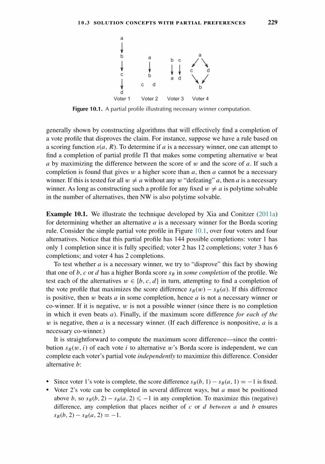
1 0 .3 solution concepts with partial preferences 229
Figure 10.1. A partial profile illustrating necessary winner computation.
generally shown by constructing algorithms that will effectively find a completion ofa vote profile that disproves the claim. For instance, suppose we have a rule based ona scoring function s(a, R). To determine if a is a necessary winner, one can attempt tofind a completion of partial profile � that makes some competing alternative w beata by maximizing the difference between the score of w and the score of a. If such acompletion is found that gives w a higher score than a, then a cannot be a necessarywinner. If this is tested for all w �= a without any w “defeating” a, then a is a necessarywinner. As long as constructing such a profile for any fixed w �= a is polytime solvablein the number of alternatives, then NW is also polytime solvable.
Example 10.1. We illustrate the technique developed by Xia and Conitzer (2011a)for determining whether an alternative a is a necessary winner for the Borda scoringrule. Consider the simple partial vote profile in Figure 10.1, over four voters and fouralternatives. Notice that this partial profile has 144 possible completions: voter 1 hasonly 1 completion since it is fully specified; voter 2 has 12 completions; voter 3 has 6completions; and voter 4 has 2 completions.
To test whether a is a necessary winner, we try to “disprove” this fact by showingthat one of b, c or d has a higher Borda score sB in some completion of the profile. Wetest each of the alternatives w ∈ {b, c, d} in turn, attempting to find a completion ofthe vote profile that maximizes the score difference sB(w) − sB(a). If this differenceis positive, then w beats a in some completion, hence a is not a necessary winner orco-winner. If it is negative, w is not a possible winner (since there is no completionin which it even beats a). Finally, if the maximum score difference for each of thew is negative, then a is a necessary winner. (If each difference is nonpositive, a is anecessary co-winner.)
It is straightforward to compute the maximum score difference—since the contri-bution sB(w, i) of each vote i to alternative w’s Borda score is independent, we cancomplete each voter’s partial vote independently to maximize this difference. Consideralternative b:
� Since voter 1’s vote is complete, the score difference sB(b, 1) − sB(a, 1) = −1 is fixed.� Voter 2’s vote can be completed in several different ways, but a must be positioned
above b, so sB(b, 2) − sB(a, 2) � −1 in any completion. To maximize this (negative)difference, any completion that places neither of c or d between a and b ensuressB(b, 2) − sB(a, 2) = −1.

230 1 0 incomplete information and communication
� Voter 3’s vote can be completed by placing c and d between b and a, giving completionb � c � d � a and a maximum difference of sB(b, 3) − sB(a, 3) = 3.
� Voter 4’s vote can be completed in two ways, but in each case we have a maximumdifference of sB(b, 3) − sB(a, 3) = −3.
Summing these maximum differences gives a profile that maximizes the score differ-ence sB(b) − sB(a) = −2. Hence b does beat a in any completion, so cannot be used torefute the fact that a is a necessary co-winner. (This also shows that b is not a possiblewinner).
We can apply the same reasoning to construct a profile that maximizes sB(c) − sB(a).Vote by vote it is not hard to see that the maximum possible difference between c anda is: −2 in vote 1; 2 in vote 2 (using completion c � d � a � b); 3 in vote 3 (usingcompletion c � d � b � a); and −1 in vote 4 (using completion a � c � d � b).In other words, we have a profile where sB(c) − sB(a) = 2.8 This means a is not anecessary winner (or co-winner). For completeness, we note that sB(d) − sB(a) = 0 isthe maximum difference for alternative d.
These intuitions can be translated straightforwardly into an O(nm) algorithm forcomputing completions, hence an O(nm2) algorithm for testing whether an alternativea is a necessary winner (or co-winner) (Xia and Conitzer, 2011a).
We note that in this partial profile:
� a is a possible winner: the completions a � b � c � d, b � a � c � d, a � d � c � b,of votes 2, 3, and 4, respectively, render a the unique Borda winner.
� b is not a possible winner (the detailed reasoning sketched earlier shows that b’s maxi-mum score advantage over a is negative, so b cannot beat a in any completion).
� c is a possible winner (using the completion and detailed reasoning sketched previously).� d is a possible co-winner: the completions d � c � a � b, c � d � b � a, a � d �
c � b, of votes 2, 3, and 4, respectively, give d a Borda score of 7, that is, equal to thatof both a and c and higher than that of b. Note that there is no completion that rendersd a unique Borda winner.
� There is no necessary winner, because there are at least two possible winners. �
While computing possible and necessary winners is generally easy with a boundednumber of alternatives, this is no longer the case for many rules when voters areweighted. For instance, rules such as Borda, Copeland, maximin, and veto have NP-complete possible winner problems for a bounded number of voters. We do not discussweighted models in depth, but refer to recent work by Conitzer and Sandholm (2002),Walsh (2007), and Lang et al. (2012b) for a selection of results using this model.
10.3.2 Minimax Regret
While possible and necessary winners are valuable concepts for providing (normative)constraints on the decisions one might make given a partial profile, they do not providea general means for selecting winners given arbitrary partial profiles. Specifically,
8 It is easy to verify that c also has a higher score than both b and d in this completion—hence c is a possiblewinner.
1 0 .3 solution concepts with partial preferences 231
necessary winners generally will not exist without a substantial amount of preferenceinformation, while possible winners can only be used to narrow the set of alternatives. Incircumstances when one is required to make a decision without complete information—or where the cost of obtaining further preferences outweighs the benefit—the followingquestions remain: which of the possible winners should one select? and is it reasonableto select an alternative that is not a possible winner?
Lu and Boutilier (2011c) propose the use of minimax regret to address this problem.9
Assume a voting rule f defined using some scoring function s(a, R). In this section,we treat this score as a measure of societal “utility” or social welfare. Given a partialprofile �, the quality of a proposed winning alternative a under � is defined to be thedifference between the score of a and the score of the winner (i.e., alternative withthe optimal score), in the worst case (i.e., given any completion of �). The minimaxoptimal alternative is that which is closest to optimal in the worst case. More formally,define:
Regret(a, R) = maxa′∈A
s(a′, R) − s(a, R) (10.1)
= s(f (R), R) − s(a, R),
PMR(a, a′, �) = maxR∈C(�)
s(a′, R) − s(a, R), (10.2)
MR(a, �) = maxR∈C(�)
Regret(a, R)
= maxa′∈A
PMR(a, a′, �), (10.3)
MMR(�) = mina∈A
MR(a, �), (10.4)
a∗� ∈ argmin
a∈A
MR(a, �). (10.5)
Here Regret(a, R) is the loss (or regret) of selecting a as a winner instead of choosingthe true winning alternative under rule f (or scoring function s). PMR(a, a′, �) denotesthe pairwise max regret of a relative to a′ given partial profile �, namely, the worst-caseloss—under all possible realizations of the full profile—of selecting a rather than a′.The maximum regret MR(a, �) is the worst-case loss associated with a, assuming anadversary selects some completion R of � to maximize the loss between the selectedalternative a and the true winner under R. The goal is thus to find the a with minimummax (minimax) regret: here MMR(�) denotes minimax regret under partial profile �,while a∗
� denotes the minimax optimal alternative. Note that the minimax winner maynot be unique (indeed, given a complete profile R several alternatives may be tied withthe best score, requiring some form of tie-breaking).
Measuring the loss of choosing an incorrect alternative using scores in this way isnot without controversy, but has been used in other contexts; for example, Smith (2000)
9 Minimax regret was proposed by Savage (1951) as a means for making decisions in the context of strict (ornonprobabilistic) uncertainty over world states. It has since been advocated for robust decision making withpartial preference or utility functions in both single-agent and multiagent settings; see Boutilier (2013) for anoverview.
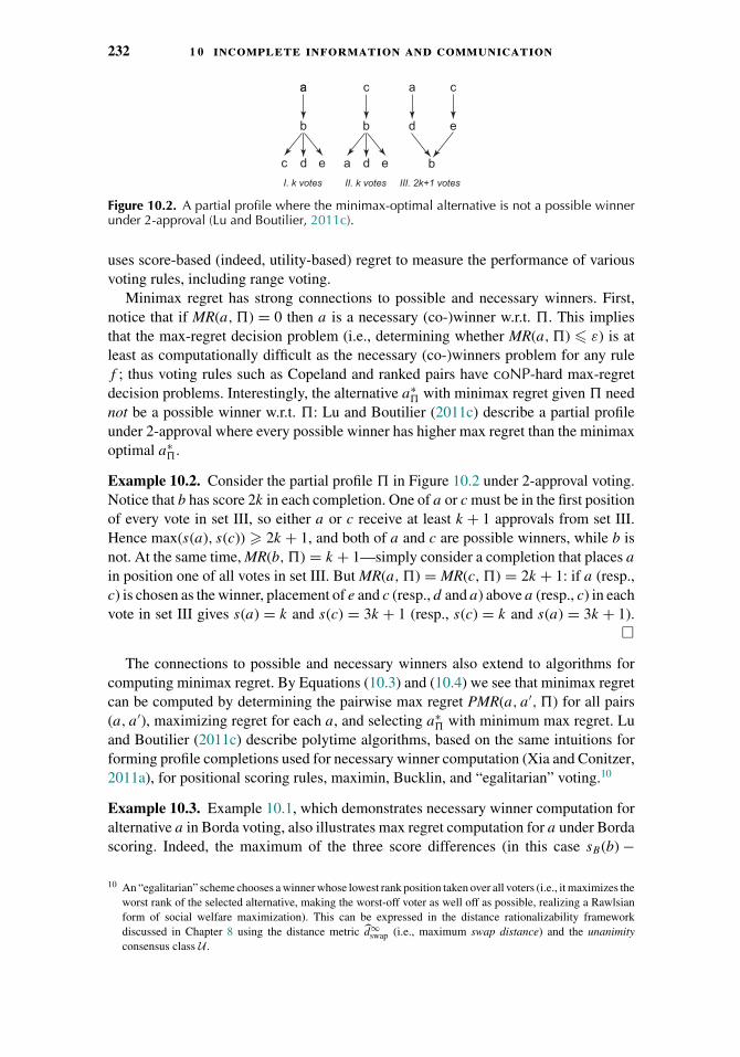
232 1 0 incomplete information and communication
Figure 10.2. A partial profile where the minimax-optimal alternative is not a possible winnerunder 2-approval (Lu and Boutilier, 2011c).
uses score-based (indeed, utility-based) regret to measure the performance of variousvoting rules, including range voting.
Minimax regret has strong connections to possible and necessary winners. First,notice that if MR(a, �) = 0 then a is a necessary (co-)winner w.r.t. �. This impliesthat the max-regret decision problem (i.e., determining whether MR(a, �) � ε) is atleast as computationally difficult as the necessary (co-)winners problem for any rulef ; thus voting rules such as Copeland and ranked pairs have coNP-hard max-regretdecision problems. Interestingly, the alternative a∗
� with minimax regret given � neednot be a possible winner w.r.t. �: Lu and Boutilier (2011c) describe a partial profileunder 2-approval where every possible winner has higher max regret than the minimaxoptimal a∗
�.
Example 10.2. Consider the partial profile � in Figure 10.2 under 2-approval voting.Notice that b has score 2k in each completion. One of a or c must be in the first positionof every vote in set III, so either a or c receive at least k + 1 approvals from set III.Hence max(s(a), s(c)) � 2k + 1, and both of a and c are possible winners, while b isnot. At the same time, MR(b, �) = k + 1—simply consider a completion that places a
in position one of all votes in set III. But MR(a, �) = MR(c, �) = 2k + 1: if a (resp.,c) is chosen as the winner, placement of e and c (resp., d and a) above a (resp., c) in eachvote in set III gives s(a) = k and s(c) = 3k + 1 (resp., s(c) = k and s(a) = 3k + 1).
�
The connections to possible and necessary winners also extend to algorithms forcomputing minimax regret. By Equations (10.3) and (10.4) we see that minimax regretcan be computed by determining the pairwise max regret PMR(a, a′, �) for all pairs(a, a′), maximizing regret for each a, and selecting a∗
� with minimum max regret. Luand Boutilier (2011c) describe polytime algorithms, based on the same intuitions forforming profile completions used for necessary winner computation (Xia and Conitzer,2011a), for positional scoring rules, maximin, Bucklin, and “egalitarian” voting.10
Example 10.3. Example 10.1, which demonstrates necessary winner computation foralternative a in Borda voting, also illustrates max regret computation for a under Bordascoring. Indeed, the maximum of the three score differences (in this case sB(b) −
10 An “egalitarian” scheme chooses a winner whose lowest rank position taken over all voters (i.e., it maximizes theworst rank of the selected alternative, making the worst-off voter as well off as possible, realizing a Rawlsianform of social welfare maximization). This can be expressed in the distance rationalizability frameworkdiscussed in Chapter 8 using the distance metric d∞
swap (i.e., maximum swap distance) and the unanimityconsensus class U .

1 0 .3 solution concepts with partial preferences 233
sB(a) = 2) is precisely the max regret of alternative a under the partial profile inquestion. Computing max regret for all four alternatives shows that minimax regret canbe computed in O(nm3) time for Borda scoring. In this example, a is the minimax-optimal alternative. �
10.3.3 Probabilistic Solution Concepts
A different approach to the analysis of winners with partial information uses probabilis-tic information about voter preferences. Notice that possible and necessary winners arepurely epistemic notions that do not prescribe a general method for choosing winnersunder partial profiles. Minimax regret does provide a general method for selecting win-ners in such circumstances, but quantifies loss using a worst-case analysis, ignoring theprobability of specific completions. By contrast, at least in cases where probabilisticpreference models are available, a more refined analysis of the likelihood of variouscompletions can be used to make decisions.
Naturally, probabilistic models have been used extensively in the analysis of voting,but typically they are used to assess the odds of certain phenomena arising in (completeknowledge) voting settings under specific culture or other preference assumptions. Forexample, theoretical and empirical analysis of the probability of a Condorcet cycleoccurring in a vote profile are very common (Gehrlein and Fishburn, 1976; Regenwetteret al., 2006; Mattei, 2011). Probabilistic models are used to study, both theoreticallyand empirically, the probability that manipulation opportunities can arise in electionsas well as to offer average-case analysis of the computational hardness of manipulation(see Chapter 6 or Faliszewski and Procaccia (2010) for an overview). Such models arealso required to analyze voting equilibria (i.e., Bayes-Nash equilibria in the incompleteinformation game played by strategic voters against one another; Majumdar and Sen,2004; Angel Ballester and Rey-Biel, 2009), and have been used to analyze the expectedloss induced by the use of voting rules under certain social welfare measures (Hillinger,2005; Smith, 2000) (see connections to our discussion in Section 10.8).
Here we focus on the probabilistic analysis of partial profiles, which can be usedto answer several important questions. The probabilistic analog of the possible winnerproblem is computing the probability Pr(win(a)|�) that a specific alternative a winsunder a voting rule f given partial profile �. Bachrach et al. (2010b) consider arestricted form of this problem—counting the number of completions in C(�) ofpartial profile � for which a is the winner, which they dub #PW. Given that countingthe number of linear extensions of a partial order is #P-hard (Brightwell and Winkler,1991), they show that #PW is also #P-hard for plurality and veto. However, they alsoprovide a polytime (randomized) approximation algorithm for #PW that can be usedfor any voting rule for which winner determination is polytime solvable. By samplingcompletions uniformly at random (which can be done in polynomial time), and apply-ing Hoeffding bounds to determine the requisite number of samples, they prove that thefraction of sampled profiles in which a wins is close to the true fraction of such comple-tions with high probability. This work is restricted in that it assumes voter preferencesare independent and drawn from a uniform distribution (i.e., impartial culture).
Hazon et al. (2012) consider a model that allows for arbitrary distributions of voterpreferences (though they still assume independence of voter preferences) and provide a

234 1 0 incomplete information and communication
general dynamic programming algorithm to compute the probability that (any) a winsunder a variety of voting rules under fairly general circumstances. For example, givena constant-bounded number of alternatives and weighted votes—where weights arethemselves polynomially bounded in n—they show that computing the probability ofan alternative winning is polytime solvable for any voting rule with polytime winnerdetermination. The dynamic programming model uses a compact representation ofvoting scenarios tightly tied to work on compilation complexity (see Section 10.7).The approach assumes that each voter i’s distribution is given in explicit form; thatis, a probability is specified for each possible ranking the voter may hold (e.g., onefor each �i∈ C(πi)). This representation is straightforward when m is small, butbecomes problematic for larger m, where prior distributions are usually representedusing parametric distributions, and for which conditioning on partial preferences isoften intractable (Lu and Boutilier, 2011b). Much like Bachrach et al. (2010b), whenthe number of alternatives is taken as a parameter, Lu and Boutilier (2011b) showthe problem to be #P-hard for k-approval, Borda, Copeland, Bucklin, and plurality.For such larger problems, they propose using a sampling approach to estimate theprobability that a specific a wins, treating this as a binomial experiment and providingconfidence bounds (in contrast to the Hoeffding approach used by Bachrach et al.(2010b)).
Computing the probability that specific alternatives win, just like computing pos-sible winners, may not be sufficient to support selection of a winner given a partialprofile �. Given a partial profile �, the probabilistic approach can be combined withthe decision-making capabilities of score-based voting or regret-based optimization tomake decisions that exploit distributional information. For example, given a partial pro-file �, the dynamic programming and sampling algorithms of Hazon et al. (2012) couldbe adapted, or in some cases used directly, to compute the expected score or expectedregret (assuming a score-based voting rule) of each alternative, allowing Bayesian-optimal winners to be chosen given �. Suitable sample-complexity results would needto be derived to provide confidence in the results. Lu and Boutilier (2011d) take sucha decision-making perspective on the use of probabilistic models, but use this to drivea particular elicitation process (see Section 10.5). This probabilistic, decision-makingperspective is also adopted in the analysis of manipulation given partial vote profilesoffered by Lu et al. (2012). However, in general, truly decision theoretic analysis of vot-ing and preference aggregation mechanisms remains a relatively under-studied topic.
10.4 Communication and Query Complexity
One of the main reasons to implement social choice functions with partial profilesis to minimize the amount of information needed to reach a group decision. Whilethe previous section described several techniques for making decisions given a specificpartial profile, in this section and the next we describe techniques for eliciting the “right”(partial) preference information needed to implement a voting rule. In this section weoverview formal models of communication and query complexity that quantify theamount of information needed in the worst case to realize specific voting rules. In the

1 0 .4 communication and query complexity 235
next section, we turn our attention to more practical, heuristic elicitation methods thattend to reach correct (or good) decisions with relatively small amounts of preferenceinformation.
Formal models of the communication demands of voting rules come in two varieties.One approach uses the tools of communication complexity (Yao, 1979; Kushilevitz andNisan, 1996), measuring the number of bits of information that need to be commu-nicated by voters to the voting mechanism before a winner can be determined usingsome voting rule. The other approach measures the number of queries that voters needto answer in order to allow the determination of a winner. In this model, results canbe very sensitive to the precise form of query used, since certain queries may carrysignificantly more information than others. Notice, however, that some queries maybe more or less natural for voters, and more or less difficult to answer—their cog-nitive complexity may not stand in direct relation to the information they carry (inbits), and may vary from one voter to another.11 Naturally, bounds on the number ofqueries needed can be translated directly into upper bounds on communication com-plexity by simply using the number of bits needed to respond to a query of the type inquestion.
Before outlining these models, we list several natural forms of queries that can beused to communicate information about voter preferences:
� Full ranking queries: a voter i provides her entire ranked list of alternatives �i .� Set ranking: voter i is asked to rank all alternatives (w.r.t. each other) in a subset S ⊆ A.
If S = A, this corresponds to a full ranking.� Top-k queries: i provides the top k (ranked) alternatives from �i for some 1 � k � m.
Notice that setting k = 1 corresponds to plurality, while the use of full ranking queriescorresponds to setting k = m (or k = m − 1). Bottom k queries can be defined similarly.
� Next-best-alternative queries: in sequential elicitation schemes, voter i can be asked tostate her “next most preferred alternative;” the kth such query asks for her kth-rankedalternative, assuming that the first k − 1 have already been provided (the completeinformation set corresponds to answering a top-k query).
� Pairwise comparisons: voter i is asked to state which of two alternatives, a or a′, ispreferred to the other.
� Set choice: voter i is presented with a subset S ⊆ A, and asked which alternative in S
is most preferred. If |S| = k, the response is equivalent to answering (a specific set of)k − 1 pairwise comparisons.12
� Positional: voter i is asked which alternative is ranked in position t in her ranking �i .� Approval: voter i is asked to approve of any number of alternatives, or a fixed number k
of alternatives. For fixed k-approval, such queries are similar to top k queries in that the
11 For instance, a pairwise comparison of the form “do you prefer a to a′?” may be more difficult for a voter whois almost indifferent between the two than for a voter who strongly prefers one of the two and strongly dislikesthe other. Yet both responses can be communicated to a voting mechanism using one bit. Certain psychometricmodels of choice (e.g., the Luce-Shepard model (Luce, 1959; Shepard, 1959)) capture choice “errors” that areexponentially less likely the more distinguishable two alternatives are w.r.t. their utility.
12 Specifically, if a ∈ S is revealed as most preferred, this response contains the same information as the k − 1comparisons: a � a′, for all a′ ∈ S \ {a}. Of course, one cannot determine which k − 1 pairwise comparisonswould “simulate” this set choice prior to the received response.
236 1 0 incomplete information and communication
top k alternatives are identified, but differ because these are not ranked relative to oneanother. Veto is defined analogously and bears the same relation to bottom k queries;and for a fixed k, k-veto is equivalent to (m − k)-approval.
� Split queries: voter i is asked to partition a subset S ⊆ A into two or more blocks ofalternatives, each of some specified size, and an ordering of these blocks, such that eachalternative in a higher ranked block is preferred to all alternatives in any lower rankedblock. k-approval is a special case where two blocks are used of sizes k and m − k.
Conitzer and Sandholm (2005b) study the communication complexity of a varietyof common voting rules using the standard model used in the study of distributedalgorithms (Yao, 1979; Kushilevitz and Nisan, 1996). A protocol that implements avoting rule can be interpreted (somewhat informally) as follows: each voter i has aninput �i corresponding to its ordering of alternatives, and the collection of voters wantsto compute the function f (R), where R is the profile and f is the voting rule in question.A (deterministic) protocol proceeds in stages: at each stage, one voter i reveals a singlebit of information based on her ranking, where the choice of voter and the bit revealedare dependent on all bits revealed at prior stages. The process terminates when theoutput f (R) of the voting rule can be determined (i.e., the bits revealed are sufficientto determine a necessary winner). The (deterministic) communication complexity ofa voting rule f is the number of bits required by the best (information minimizing)protocol in the worst case (i.e., given the input profile R that maximizes the number ofbits communicated through this protocol). Nondeterministic protocols can be definedsimilarly.
To determine upper bounds on the communication complexity of a voting rule,Conitzer and Sandholm (2005b) provide deterministic protocols that realize the rule.For example, a universal upper bound of O(nm log m) bits is easy to see for any rank-based rule: each voter can communicate the rank (one of m positions) of each of m
alternatives using log m bits. An upper bound of O(n log m) for plurality is easy tosee since each voter need only communicate the identity (using log m bits) of its mostpreferred alternative. We discuss additional upper bounds later.
Lower bounds are shown for many voting rules using the fooling set technique: afooling set of size k for rule f is any set of k distinct profiles R1, . . . , Rk—whereeach Rj = 〈�j
1, . . . ,�jn〉—such that for each i � k, f (Ri) = a for some a ∈ A (i.e.,
each profile has the same winner); but for any i, j � k there is some mixture of thetwo profiles of the form Rij = 〈�x
1, . . . ,�xn〉, where �x
=�i or �x
=�j , such that
f (Rij ) �= a. If such a fooling set exists, then the communication complexity of f is atleast log k. This must be so since any protocol must distinguish each pair of inputs inthe fooling set (Kushilevitz and Nisan, 1996): if it failed to distinguish Ri from Rj , itcould not tell if the input profile was actually Rij and thus could not in fact implementf . By constructing fooling sets of the appropriate size, lower bounds are provided ona variety of rules.
For many rules, Conitzer and Sandholm (2005b) are able to provide matching lowerand upper bounds: for plurality (including with runoff), O(n log m) and �(n log m); andfor Borda, ranked pairs and Copeland, �(nm log m), which matches the universal upperbound. Other rules analyzed include maximin, approval, cup, Bucklin and Condorcet,

1 0 .4 communication and query complexity 237
which have upper bounds of O(nm) and lower bounds of �(nm); and STV, which isO(n(log m)2) and �(n log m).13
To illustrate, we outline the proof sketch of Conitzer and Sandholm (2005b) demon-strating the O(mn) upper bound for Bucklin (which is tighter than the universalO(nm log m) upper bound). Recall that the (simplified) Bucklin rule chooses as thewinner the alternative a such that a lies within the top l positions of the rankings of atleast half of the voters for the minimum value of l for which the property holds (seeChapters 2–4).
Proof sketch. The following protocol for Bucklin essentially performs a binary searchfor the minimum value l � m such that at least half of the voters rank some a
within the top l positions, maintaining upper and lower bounds U, L on this posi-tion. Given the current upper and lower bounds (initialized at m, 0 resp.), we needto test whether k = !(U + L)/2" > l (and update the appropriate bound based on theanswer). To do so, we can ask each voter to report, for each alternative a, whethera lies within the top k positions of their ranking. This can be answered with m bitsper voter (a yes-no response for each alternative); and since the binary search requiresat most log m iterations, this straightforward approach requires at most O(nm log m)bits.
However, the number of bits required per voter can be cut in half at each iteration.Simply observe that at any iteration t + 1, the past responses of voter i reveal theidentities of 2t−1
2t m alternatives that lie above or below the queried threshold k at thatiteration. For example, the first query asks each voter to indicate which alternatives arein their top m/2 positions. Suppose we determine l � m/2, so that each voter is nextasked to reveal which alternatives lie in their top m/4 positions: since in response tothe prior query, each voter indicated m/2 alternatives that lie outside their top half,these same m/2 alternatives must also lie outside their top quarter. Hence at iterationtwo, each voter needs to reveal only m/2 bits (denoting which alternatives in their tophalf also lie in their top quarter). Ignoring rounding due to imperfect splitting, we havethat each voter reveals
∑log mt=0
12t m � 2m bits in total. This proves the upper bound of
O(nm) bits. �
The communication complexity of determining approximate winners is also ofinterest. For instance, for voting rules defined using natural scoring functions, wecan use the score difference between alternatives as a measure of approximation asdiscussed in Section 10.3.2; it may be that the communication complexity of approxi-mate winner determination is less than that of exact winner determination. Service andAdams (2012b) analyze several voting rules in this fashion. Borda voting, for exam-ple, can benefit from approximation—the communication complexity of determininga (1 − ε)-approximate winner is O( 1
εnm), which stands in contrast to the �(nm log m)
13 The cup voting rule is essentially a tournament specified by a balanced binary tree. Each alternative is initiallyassigned to a single leaf. Each pair of siblings (children of the same parent in the tree) “face off” againsteach other in a pairwise election, with the winner assigned to the parent. The winner of the tournament is thealternative assigned to the root of the tree.
238 1 0 incomplete information and communication
needed for exact winner determination described earlier.14 By contrast, they show thatapproximating Bucklin to degree ρ requires �(nm
ρ2 ) communication, meaning that anyconstant factor approximation offers little savings in the worst case relative to exactwinner determination (which is O(nm)). They also provide an analysis of Copelandand consider several nonconstant approximation bounds.
An example using a slightly different model of query complexity, rather than directcommunication complexity, is provided by Procaccia (2008). He analyzes the num-ber of queries needed to determine a Condorcet winner, where each query is allowedto ask about the existence of a directed edge between two alternatives in the tour-nament graph induced by a profile R. Notice that the answer to such a query doesnot provide direct information about the preferences of any individual voter—thus,a set of such responses does not correspond to a partial profile under our precedingdefinition. However, it still constrains possible vote profiles. Procaccia shows that aCondorcet winner can be determined using 2m − log m − 2 such edge queries. Sinceeach edge query could be determined by asking each of the n voters to answer a singlepairwise comparison query, this provides an upper bound of O(nm) on communica-tion complexity. He also provides a matching lower bound on the number of edgequeries (note, however, that this does not provide a lower bound on communicationcomplexity, since the analogous �(nm) bound only applies if one is restricted to edgequeries).
A very different axiomatic perspective on the complexity of communication isprovided by Sato (2009). He considers the number of distinct messages each voter cansend in various (one-shot) protocols associated with specific voting rules and considersthe impact of minimizing the number of messages allowed. Define the informationalsize of a voting rule to be the total number of distinct messages (across all voters)that can be sent (e.g., the information size of plurality is nm since each of n voterscan send one of m messages). Assume that each voter preference determines a uniquemessage (hence messages partition the space of orderings or preferences R(A)). Satothen characterizes the voting rules that are informationally minimal, with respect totheir informational size, among all rules satisfying certain combinations of axiomaticproperties. As one example, he shows that among (nontrivial) anonymous, neutral andmonotonic voting rules, only those (loosely) corresponding to either plurality or vetoare informationally minimal. This perspective is somewhat different than that takenabove in that (a form of) informational complexity is being suggested as a property bywhich one might choose to use one voting rule rather than another, in the same spiritas much axiomatic analysis of voting.
When voter preferences have special structure, specific mechanisms can be usedto exploit this structure for a variety of purposes. One of the most widely studiedsuch structures is single-peakedness (Black, 1948) for which the median mechanismand various generalizations are strategyproof, and require that voters simply revealtheir most preferred alternative rather than their entire ranking (see Chapters 2 and 6for further discussion of single-peaked preferences). While single-peaked preferences
14 Service and Adams (2012b) derive multiplicative approximation ratios, rather than the additive error used todefine max regret in Section 10.3.2. Hence, a ρ-approximate winner a is one whose (Borda, or other) scoreratio w.r.t. the true winner w satisfies s(a)/s(w) � ρ.
1 0 .5 preference elicitation 239
and the median mechanism already support making decisions with relatively littleinformation, Conitzer (2009) addresses the communication complexity of additionalvoting problems when preferences are single-peaked. He considers several differentsettings, including cases where voter preferences are both ordinal and cardinal (e.g.,determined by some distance metric), and the axis (i.e., positions of the alternatives)may be known or unknown a priori. Restricting our attention to the case of ordinalpreferences with a known axis, he first observes that the median rule can be implementedwith n log m (pairwise comparison) queries using a binary search to determine eachvoter’s most preferred alternative—all that is needed to determine the median—givingan O(n log m) upper bound on communication complexity. Determining a voter’scomplete ranking can be accomplished with O(m) queries, with log m queries neededto determine the peak and m − 1 queries needed to “interleave” the induced left andright subrankings. He also addresses the problem of determining the full tournamentgraph (which, assuming n is odd, is acyclic and can be interpreted as a consensusranking). He shows that this requires �(nm) queries, and thus essentially requiresenough information to construct each voter’s ranking.15
10.5 Preference Elicitation
In the previous section, we discussed several forms of analysis that provided upper andlower bounds on the number of queries or bits required to determine the outcome ofvarious voting rules. These theoretical analyses show the limits of what is possible;but algorithms that minimize worst-case communication complexity may sometimeselicit more information than necessary in practice. Furthermore, these analyses donot address the informational complexity of determining decisions (or winners) that“approximate” the optimal decision (one exception is the work of Service and Adams(2012b)). In this section, we discuss approaches to preference elicitation that are drivenby more practical considerations, although several of the models also offer theoreticalanalyses of these practical aims (e.g., how much information is needed to determineapproximate winners, or true winners with high probability).
10.5.1 Incremental and Partial Preference Elicitation
The abstract goal of any preference elicitation technique is to elicit a partial profile fromvoters with “just enough” information to determine a winning outcome of “sufficientlyhigh quality.” The notion of “just enough” information can be measured formally usingthe communication or query complexity measures described in the previous section.Many of the methods discussed in this section focus on heuristic minimization ofquery complexity. More critically, elicitation schemes may use different measures forthe quality of the resulting outcome selected using the elicited partial profile. Amongthe elicitation goals considered in this section are the following:
15 Lackner (2014) considers the problem of determining whether a partial profile can be completed in such a waythat it is single-peaked, showing that it is computationally difficult in general, but providing polytime methodsfor specific classes of partial profiles.

240 1 0 incomplete information and communication
� determining the optimal outcome (i.e., a winner or a necessary co-winner) w.r.t. theunderlying (complete) vote profile
� determining the optimal outcome (i.e., true winner) with high probability� determining an outcome that is close to optimal (e.g., has low max regret)� determining an outcome that is close to optimal with high probability
Each of the models described in what follows assumes one (or more) of these abstractobjectives, and uses specific metrics to formalize decision quality and error probability.
10.5.2 The Computational Complexity of Preference Elicitation
One early line of research in vote elicitation deals with the computational complexityof various elicitation questions. Conitzer and Sandholm (2002) consider two classes ofelicitation schemes, with a focus on determining the true winner (no approximation,no probabilistic guarantees). Coarse elicitation methods are restricted to asking a voterfor her entire preference ranking or vote. The aim in coarse elicitation is to minimizethe number of voters who provide their votes while still determining the true winner.By contrast, fine elicitation schemes can ask more general queries, for example, of theform described in Section 10.4—abstractly, a query corresponds to some partitioningof the space R(A) of votes, with each response selecting some element of the partition(those votes consistent with the response).
Conitzer and Sandholm analyze two main classes of computational questions. Elic-itation Not Done (END) asks, given a partial profile consisting of the votes from asubset S ⊆ N of voters and an alternative a, can the remaining votes be cast so thata loses. This question anticipates subsequent developments in the theory of possibleand necessary winners: if the answer is no, a must be a necessary co-winner, and incertain circumstances this may be sufficient to terminate the vote elicitation proce-dure. Indeed, the problem is equivalent to the necessary co-winner problem (given thisrestricted form of partial profile).16 They show that END is NP-complete for STV, evenwhen the partial profile consists of all votes but one (exploiting a result of Bartholdiand Orlin (1991), see Section 10.3.1). Since the result is cast in terms of coarse elic-itation, it naturally applies to any fine elicitation scheme that can simulate coarseelicitation (as most would). They show, by contrast, that END can be solved in poly-nomial time for plurality, Borda, Copeland, approval and maximin (for fine or coarseelicitation).
They consider a second problem as well: Effective Elicitation (EE) asks whether,given a partial profile of votes from S ⊆ N , there is a subset of the remaining voters,of size at most k, whose votes determine the winner. From an elicitation perspective,this question assumes the protocol knows the responses it will obtain (or has “perfectsuspicions”). While unrealistic, this suggests the computational problem given less thatperfect knowledge will be even more difficult. Conitzer and Sandholm (2002) showthat EE is NP-complete for several different voting rules, including approval, Borda,Copeland and maximin.
16 Since they cast the problem in terms of coarse elicitation, this is also equivalent to the problem of (coalitional)destructive manipulation; see Chapter 6.

1 0 .5 preference elicitation 241
Walsh (2008) continues this line of investigation, analyzing the END problem for avariety of other voting rules and considers weighted voting schemes as well. Of specialnote, Walsh shows that END is computationally easier using coarse elicitation thanfine elicitation for several different (weighted) voting rules under various conditions.For instance, END for the Cup rule is coNP-complete (with four or more alternatives)using fine elicitation, but can be solved in polynomial time if we restrict attention tocoarse elicitation.
10.5.3 Incremental Vote Elicitation
We now describe several approaches for the elicitation of voter preferences. In manycases, the methods have been analyzed empirically to assess their effectiveness in prac-tical circumstances. Several are supported by theoretical analyses as well to determinehow much information is required to reach “high quality” decisions.
Kalech et al. (2011) were among the first to develop and evaluate significant, practi-cal vote elicitation schemes that allowed the selection of winners using partial profiles.They propose two elicitation schemes designed for use with scoring-based rules (e.g.,Borda, range voting), using specific forms of queries and possible and necessary win-ners as the primary solution concept. Their first technique, dubbed Iterative Voting,17
is used to determine a true winner (no approximation) and proceeds in rounds. At eachround, each voter is queried for their next best alternative; hence by round t each voterhas (incrementally) answered a top-t query. At the end of each round, necessary andpossible winner computation on the current partial profile is used to determine termina-tion: if every possible winner is a necessary (co-)winner, the process stops and returnsthe full set of necessary winners. (The algorithm could also be terminated once anynecessary winner is found.) Empirical analysis of range voting and Borda voting, usingsmall vote profiles (up to 30 voters and 50 alternatives) generated randomly and fromreal-world ratings data, shows that this scheme can reduce the number of alternativesthe average voter has to rank by 10%–40%, with the larger gains possible when userpreferences are more uniform.
Kalech et al.’s second algorithm, Greedy Voting, proceeds for a predetermined num-ber of rounds T . Given the current partial profile �t at round t , each alternative isevaluated to determine its minimum and maximum possible scores (over all comple-tions R of �t ) relative to the scoring function s(a, R) for the voting rule in question.Then each voter is asked to rank the set of Q alternatives with the largest minimumscores (maximum scores are used to break ties), for some small Q. Since terminationis predetermined after T rounds, necessary winners may not result, so possible winnersare returned. One attractive feature of this model is the batching of queries (voters areonly queried a fixed, ideally small, number of times, though each query may requestmore information than in the other schemes discussed later). Such batching can mini-mize user interruption as well as user latency (since voters are required to wait until theresponses of other voters are delivered before their next query is received). This schemeprovides no guarantee of winner optimality or any bounds on quality, hence Kalech
17 This should not be confused with iterative schemes in which voters change their votes in response to the currentvote profile.
242 1 0 incomplete information and communication
et al. (2011) empirically evaluate the (post hoc) quality of the resulting winners relativeto the true winners that would have resulted had the full vote profile been available.18
In small domains, winner quality is shown to be relatively high and naturally improveswith the number of rounds permitted.
Lu and Boutilier (2011c) propose an elicitation scheme that exploits minimax regretto determine winners given a partial profile and that uses the solution of the MMRproblem to guide the selection of queries. Two different forms of queries are con-sidered: simple pairwise comparisons, and “next best alternative queries.” As earlier,the process proceeds in rounds. Let �t be the partial profile at round t with minimaxregret MMR(�t ) and minimax optimal solution a∗ = a∗
�t . Let a′ be an alternative thatmaximizes the regret of a∗, that is, an a′ that maximizes Equation 10.3. This a′ is an“adversarial witness” that has maximum advantage (w.r.t. scoring function s) over a∗
in the worst-case.If MMR(�t ) falls below some threshold τ , elicitation can stop and an approximate
winner (with an additive error bound of τ ) is returned. Thus the Lu-Boutilier schemesupports approximate winners (note that setting τ = 0 guarantees true winners arereturned). If not, a query is selected that will refine the partial profile. They propose acurrent solution heuristic for selecting queries. Specifically, the alternatives a∗ anda′ are used to identify: (i) the voter for whom the worst-case profile completionprovides the maximum “controllable” advantage of a′ over a∗, where the advantageis controllable if it can be reduced using a different completion; and (ii) a pairwisecomparison query such that a positive response would provide the greatest reductionin that advantage.19 They provide techniques for effectively determining these queriesfor positional scoring rules.
Example 10.4. In Example 10.1 (see discussion in Example 10.3) a’s max regret is 2(it is easy to verify that a is minimax optimal). A query to voter 3 that asks if a � c, ifanswered positively, reduces c’s advantage over a in vote 3 from 3 to −1, thus reducingPMR(a, c) from 2 to −2 and the max regret of a from 2 to 0, hence proving a is anecessary (co)-winner. �
Lu and Boutilier (2011c) evaluate their method, using Borda voting, on both ran-domly generated and real-world preference and electoral data sets (with up to 20 itemsand up to 5000 voters). They show that on the real-world data sets, the current solutionscheme can reduce the number of queries needed to find the true winner by 50%–65%relative to the number of (comparable) queries needed to construct the entire profile;and on synthetic Mallows profiles they show that reductions of up to 80% are possiblewhen preferences are very correlated; but even 25% reductions are possible under fullyrandom (impartial culture) preferences. Just as importantly, their scheme has the abilityto provide approximate winners with provable quality guarantees. Indeed, approximatewinners with low max regret can be found using a small fraction of the queries neededto find the true winner.
18 Note that this is possible only in experimental situations. In any practical deployment, the true profile will beunavailable and no such evaluation is possible.
19 For next-best-alternative queries, no choice of query needs to be made, only choice of a voter.
1 0 .5 preference elicitation 243
Other approaches to incremental vote elicitation exploit the use of probabilisticmodels of voter preferences (e.g., Goel and Lee, 2012; Dery et al., 2010). We examinetwo other models that exploit probabilistic models in the next section.
One drawback of the Lu-Boutilier scheme is that it asks one query of a single voterat each round. By contrast, the scheme of Kalech et al. (2011) asks all voters to answera particular query simultaneously, and (at least in the Greedy Voting scheme) can varythe granularity of that query to effectively reduce the number of rounds. In essence,there are important trade-offs among several key metrics that should addressed whendesigning practical elicitation schemes:
1. Winner quality: approximating the winner usually allows for less preference information,but at the cost of outcome quality.
2. Amount of information elicited: higher quality outcomes and fewer rounds of elicitationcan usually be achieved at the cost of additional preference information.
3. Number of rounds of elicitation: multiple rounds of elicitation can often reduce theamount of information needed to reach a decision of the same quality by conditioningqueries on past responses. However, additional rounds of elicitation impose costs interms of interruption, cognitive/context switching and latency (voters waiting on theresponses of other voters).
Lu and Boutilier (2011d) develop a general framework for framing these trade-offsusing multiround elicitation protocols. They evaluate this model in the specific contextof single-round protocols, as we discuss next.
10.5.4 One-Shot Partial Vote Elicitation
Lu and Boutilier (2011d) address the question of whether high quality winners (asmeasured using max regret) can be guaranteed using a single round of elicitation. Inmore detail, they ask whether one can determine a value k such that asking a top-k queryof every voter allows one to determine an approximate winner with low max regret(assuming a scoring-function based voting rule that admits max regret computation).In general, such guarantees are not possible in the worst-case for most voting rules(see Section 10.4), so they assume that voter preferences (or vote profiles if voterpreferences can be correlated) are drawn according to some distribution P . Rather thanassuming a specific form of the distribution, they assume only that it can be sampledeffectively. They then defined a sampling procedure that determines the minimumvalue of k such that top-k voting results in a profile with low minimax regret (hence analternative that is an approximate winner) with high probability. Specifically, given adesired solution accuracy ε > 0, solution confidence δ > 0, sampling accuracy ξ > 0,and sampling confidence η > 0, they determine the number of sampled profiles thatmust be drawn to determine an empirical estimate of k that ensures that if a top-k partialprofile �[k] is elicited, then P [MMR(�[k]) � ε] > 1 − δ − 2ξ (where the number ofsampled profiles is proportional to ln 2m/η and 1/ξ 2). Empirically, they show thatthe sampling approach can be used not only to determine the appropriate value of k
for top-k voting, but also to assess the trade-offs between the amount of preferenceinformation elicited (value of k) and the distribution over solution quality (resultingMMR).

244 1 0 incomplete information and communication
Oren et al. (2013) also analyze top-k voting, but rather than sampling profiles froman unknown distribution, they assess the values of k needed to ensure the true winneris found with high probability for specific preference distributions. Their focus is onasymptotic analysis, specifically whether top-k voting determines a correct winner withprobability approaching 1 as the number of alternatives m (and indirectly, the number ofvoters n) increases.20 They show that top-k voting may not offer significant savings forBorda voting under impartial culture—they provide a lower bound of k = �(m/ log m)(for n sufficiently large relative to m). They also consider the extreme case of zero-elicitation protocols: assuming voter preferences are drawn from a Mallows model,under what conditions will selecting the alternative at the top of the (modal) referenceranking be the winner with high probability? In other words, can setting k = 0 stilldetermine the true winner? They provide a bound on the number of voters requiredto ensure this holds that depends logarithmically on m and in a complex way on φ
(the Mallows dispersion parameter). For distributions that are not too uniform (say,φ � 0.75), relatively few voters are needed to ensure zero elicitation works.
It is also interesting to consider the difficulty of the possible and necessary winnerproblems for restricted classes of partial preferences, such as those of the top-k form.For certain voting rules, these restricted problems may be computationally easierthan with unrestricted partial profiles. Baumeister et al. (2012a) explicitly considertruncated ballots of the top-k form, the bottom-k form, as well as “doubly truncated”votes (with top and bottom segments provided). They discuss the relationship of thepossible winner problem for these forms of truncated ballots to each other and to theunweighted coalitional manipulation problem.21
10.6 Voting with an Uncertain Set of Alternatives
We now turn our attention to the incompleteness or uncertainty regarding the setof alternatives A that may be available for selection by our voters N . As we’ve seen,several key questions regarding incomplete preferences are related to strategic questionsof misreporting and manipulation. Similarly, models in which alternatives may or maynot materialize are closely related to strategic questions regarding control by adding ordeleting alternatives (see Chapter 7) and questions of strategic candidacy (Dutta et al.,2001). We only briefly mention such connections in this section, but refer to Chapter 7for deeper discussion of such strategic considerations.
In this section, we generally assume that the set of alternatives A is a “potential set,”but that some of the alternatives may in fact be unavailable for selection by voters.Voter preferences are defined over the entire potential set A, but the voters are uncertainas to which alternatives are in fact available at the time they vote. The question is howvoting mechanisms should be modified or analyzed under such conditions.
20 They add the wrinkle of considering determining winners when alternatives may become “unavailable” (asdefined in Section 10.6), which means that, even in plurality voting, voters may need to provide more than theirtop alternative to ensure a feasible winner is found. We ignore this variation here. They also provide severalworst-case analyses.
21 They also describe various other forms of manipulation and campaigning in such cases, but this analysis is lessrelevant here.

1 0 .6 voting with an uncertain set of alternatives 245
Several motivations can be offered for models of this type. In labor markets, alter-natives may declare themselves eligible for multiple positions, but hiring committeedecisions may require voting (or aggregating preferences) over interviewed candidateswho may ultimately take jobs elsewhere. In some group decision contexts, determiningthe availability or feasibility of specific alternatives may be quite costly (e.g., callingrestaurants to see if reservations are possible; planning a public project or family vaca-tion to determine whether it satisfies feasibility, time and budget constraints). In thesecases, it often makes sense to cast votes to determine the most preferred (or reason-able consensus) alternatives prior to investing time, effort or money to determine thefeasibility of options that may not be selected given voter preferences.
Lu and Boutilier (2010) develop the unavailable candidate model to capture suchsituations. In this model, the set of available alternatives V ⊆ A is unknown at the timevotes are cast. Assume a distribution P over 2A, where P (V ) is the probability that V
is the true set of available alternatives. Given a vote profile R and voting rule f , thefundamental difficulty is that we may have f (A) �∈ V , that is, the winner of the fullvote may not be available. Of course, one could simply collect preferences and thenapply f to the available set V once it is revealed. But in some settings this may not beviable, for example, when the availability of an alternative may only be determined bydeclaring them the winner (e.g., offering a job to a candidate, or attempting a bookingat an exclusive restaurant). Under this assumption, one can aggregate the preferencesinto a ranking policy, an ordering � of A such that each alternative will be “offered thewin” in turn until an available alternative is discovered. In other words, � is effectivelya rationalizable group choice function.
Since no nondictatorial, unanimity preserving voting rule is robust to the deletion ofnonwinning alternatives (Dutta et al., 2001), selecting alternatives in this fashion mayproduce a winner that is not in fact the true winner relative to the realized set V . This isso not just because of the restrictive nature of the rationalizable policy, but also becausethe process may never discover the true set V . For this reason, one requires methods forcomputing the policy that minimizes the expected disagreement (difference in winnerchoice) between the ranking policy and the true voting rule f , where expectation istaken w.r.t. P (V ). Lu and Boutilier (2010) show that this problem is NP-hard in certaincircumstances. As a result, they offer a polynomial-time approximation scheme (PTAS),as well as a greedy algorithm with a 1+p2
(1−p)2 approximation ratio when all alternativesare (independently) unavailable with probability p. Empirical results show this greedyalgorithm to provide excellent results in practice. Other forms of rank aggregation maynot provide good ranking policies. For instance, the Kemeny consensus of the profileR need not be a good ranking policy in general; but for large values of p, any Kemenyconsensus is close to optimal (in terms of expected disagreement), and at least oneKemeny consensus is in fact optimal (Lu and Boutilier, 2010).
Baldiga and Green (2013) independently developed a model virtually identical tothe unavailable candidate model, using rather different motivations, and also drawconnections to the Kemeny consensus.
Notice that Lu and Boutilier assume that availability can only be tested by actuallyselecting a tentative winner—hence they attempt to minimize the odds of selecting an“incorrect” winner. Boutilier et al. (2014) approach the unavailable candidate modelfrom a different perspective: they assume that testing availability is expensive, but can
246 1 0 incomplete information and communication
be accomplished without actually selecting a winner. They address the problem ofminimizing the number (or cost) of such tests needed to determine the true winner.Specifically, assume some voting rule f , a given vote profile R. Suppose the alternativeset A is partitioned into three sets: KA (known available alternatives), KU (knownunavailable), and U (unknown availability). The true available set V can be any KA ⊆V ⊆ KA ∪ U . They define a robust winner to be any a such that f (R[V ]) = a for allV ⊆ KA ∪ U , that is, a is a winner for any realizable available set V (here R[V ] isthe restriction of profile R to available set V ). Of course, determining robust winnersis difficult for some voting rules f and easy for others; as the authors point out, thisproblem has tight connections to the problem of control by candidate addition (seeChapter 7).
If no robust winner exists, then determining the true winner requires testing theavailability of certain additional alternatives until we reach a point (state of informationabout KA and KU) that admits a robust winner. Boutilier et al. (2014) develop a dynamicprogramming method that will produce the optimal (minimum cost) availability testingpolicy, as well as a myopic search technique based on decision tree induction thatheuristically minimizes the cost of the policy. They also provide simple worst-caseanalysis of the “availability test complexity” of plurality, Borda and Copeland thatshows essentially all alternatives must be tested in the worst case. They also describesimple test policies that are optimal for extreme availability probabilities.
Chevaleyre et al. (2012) study a different issue associated with alternative uncer-tainty, namely, the possible winner problem when votes are provided over some initialset of alternatives A, then a fixed number c of new alternatives are added to the set.They study the computational complexity of determining whether an alternative a ∈ A
(i.e., one of the initial alternatives) is a possible winner given the addition of the newalternatives for various voting rules—here uncertainty lies over voter preferences forthese new alternatives. Note that this problem (as in possible and necessary winnerdetermination with a known set of alternatives as discussed earlier) bears a tight con-nection to certain forms of manipulation, specifically, the notions of cloning and controlby adding candidates (see Chapter 7).
Chevaleyre et al. (2012) provide a complete classification of the family of k-approvalrules (including plurality). For k ∈ {1, 2} (i.e., plurality and 2-approval), they showthat the possible winner problem can be solved in polynomial time for any fixed c
(the construction for 2-approval uses a reduction to a max-flow problem). For k � 3and c = 2 they show that the problem can also be solved in polynomial time; but fork � 3 and c � 3, they use a reduction from 3D Matching to show that the possiblewinner problem is NP-complete. They also provide a polytime method for Bordavoting (indeed, for a more general class of scoring rules that includes Borda). Xia et al.(2011b) adopt the same model and show that several additional voting rules have NP-complete possible winner problems with new alternatives, namely, Bucklin, Copeland(with pairwise ties in voting giving a score of 0 for both alternatives), maximin andapproval.22
22 In fact, they consider several different ways in which a voter can extend her approval vote given c newalternatives. In the arguably most natural, the problem is NP-complete, while for the others it is straightforwardlypolytime solvable or a trivial problem.
1 0 .7 compilation complexity 247
10.7 Compilation Complexity
A subset of voter preferences embodies some inherent partial information regarding theultimate result of a vote. Such a subset of preferences, or partial profile �, can of coursebe held in its raw form, as the original linear orders of the subset of voters. However,several researchers have considered the idea of compressing this information into asmaller number of bits, which still represents the essence of the partial information inthat it allows one to determine the ultimate winner of an election once the remainingvotes are received (Chevaleyre et al., 2009; Xia and Conitzer, 2010b; Chevaleyre et al.,2011). The minimum number of bits required to represent this relevant information,for a given voting rule f , is called the compilation complexity of f .
There are several reasons one might want to compile a partial (or complete) voteprofile in this way. Compilation may offer privacy benefits by discarding full voter infor-mation in favor of statistical or other summaries. It may allow for faster computationof the final result once all votes become available.23 It may also ease communicationcomplexity when partial vote results from multiple locations need to be aggregated.Finally, if vote profiles need to be stored for future validation or audits, compilationmay reduce space requirements. There are also some possible drawbacks of compila-tion; for example, it may make further elicitation more costly in some circumstances,when a specific voter has to be questioned again.
Research on compilation complexity to date has largely focused on the followingquestions: the space needed for storing compiled partial voting results when the numberof remaining voters is unknown (Chevaleyre et al., 2009); the space needed when thatnumber is known along with the number who have already voted, or one or theother might be unknown (Xia and Conitzer, 2010b); and the relationship betweencompilation complexity and communication complexity (see Section 10.4) when theset of alternatives is dynamic (Chevaleyre et al., 2011).
To illustrate the main ideas behind compilation complexity, consider the summariza-tion of partial results in plurality voting. Suppose k voters, from an ultimate electorateof size n > k, have already expressed their ordered preferences among m alternatives.Since each alternative can be specified using %log m& bits, this partial vote could bestored in its raw form and used to compute the winner once the remaining votes arereceived. This very naive storage scheme required k%log(m!)& bits to store all bal-lots (namely, specifying for each voter which of m! possible permutations matchestheir vote). However, the partial input can be represented more concisely, recordingonly the number of first-place votes received by each of the m alternatives—this usesm%log(k + 1)& bits. When the remaining n − k votes are submitted, the only data thatmatters from the initial k votes for the purposes of winner computation are alternativefirst-place vote totals.
Of course, we can do even better. Rather than store all first-place vote totals, wecan normalize them by subtracting the score of the lowest-scoring alternative from allalternative scores, hence needing to represent smaller totals (assuming no alternativereceived zero votes). Moreover, if the difference between the partial votes already
23 Note that when faster computation of the final result is the primary objective, it may sometimes be useful to‘compile’ into a structure using more space.
248 1 0 incomplete information and communication
received by the front-runner and those received by the second-place alternative isgreater than the number of votes yet to be cast by the remaining n − k voters—assuming this number of votes yet to be cast is known—the ultimate result of theelection is already determined, and the only thing that needs to be stored is the identityof the winning alternative.
Based on these intuitions, we can immediately make several simple observa-tions (Chevaleyre et al., 2009). First, the compilation complexity of any voting ruleis at most k%log(m!)& bits—we simply store all voters’ votes. For any anonymousvoting rule, the compilation complexity will be at most the minimum of k%log(m!)&and m!%log(k + 1)&, since with an anonymous rule we can store, for each ballot (linearorder), the number of voters that chose it, if that requires fewer bits. A dictatorial votingrule has compilation complexity of %log m&—only the choice of the dictator needs tobe stored if she is among the original voters (and nothing otherwise).
To formalize the compilation complexity problem, following Xia and Conitzer(2010b), consider a set of voters divided into a subset of k known votes, and a sub-set of u unknown votes. The k votes, constituting a partial profile �, are summa-rized by a string of bits via a compilation function c: c(�) ∈ {0, 1}∗. For the func-tion to be an effective summary for voting rule f , if we have profiles �1 and �2,and c(�1) = c(�2), then for any profile of the remaining u votes Q it must be thecase that f (�1 ∪ Q) = f (�2 ∪ Q). We say that �1 and �2 are f -equivalent in thiscase.
The minimum number of bits required to summarize a partial profile � of a sub-electorate of size k, for a given voting rule f , u unknown votes, and m alternatives,is called the compilation complexity of f , and is denoted by Cm,k,u(f ). It reflectsthe most space-effective function c. Chevaleyre et al. (2009) also consider the casewhere u is unknown. This can be represented using the preceding notation as Cm,k,?(f )(the question mark replacing u). This is the minimum number of bits required tosummarize the profile of a sub-electorate of size k, for a given voting rule f , whenthere are m alternatives, and the remaining number of votes u is unknown.
The definition of f -equivalence establishes equivalence classes among profiles andallows one to store a partial profile by storing the index of its equivalence class. Ifg(f, k, m) denotes the number of equivalence classes for voting rule f , already-votedsub-electorate k, and m alternatives, then the compilation complexity of a voting rule f
is precisely %log g(f, k, m)&. To derive the compilation complexity for various votingrules, we can count the relevant equivalence classes for each.
Cm,k,?(f ) is related to several of the problems described in earlier sections:
1. The complexity of terminating elicitation (Section 10.5.2): is the winner already deter-mined after we have been given a subset of the votes?
2. The complexity of possible and necessary winner determination (Section 10.3.1): if wehave a set of incomplete votes (partial orders), is there an extension where a givenalternative c is the winner?
3. Communication complexity of voting rules (Section 10.4): what is the smallest numberof bits that needs to be communicated among voters and the central authority to computethe winner of an election? Note that compilation complexity can be interpreted as “one-round communication complexity” (the message being sent by the initial voters).
1 0 .7 compilation complexity 249
4. Chevaleyre et al. (2011) consider a variant of the communication complexity problem,namely, the relationship of compilation complexity and communication complexitywhen the set of alternatives is dynamic, that is, new alternatives can be added over time(see Section 10.6).
Results
It is clear that the compilation complexity of plurality is at most m%log(k + 1)& (storingthe score between 0 and k for each alternative). Chevaleyre et al. (2009) show that thiscan be improved (with an unknown number of additional voters) to⌈
log
(m + n − 1
k
)⌉.
Exploration of compilation complexity concerns variations on the basic model. Asmentioned, Chevaleyre et al. consider Cm,k,?(f ), where the remaining number of votesu (replaced by a question mark) was the only unknown. Xia and Conitzer (2010b)expand this by considering the relationship among Cm,k,?(f ), Cm,?,u(f ) (where thenumber of already-cast votes is the unknown), and Cm,k,u(f ) (where the number ofalready-cast and the number of yet-to-be cast votes are both known). Chevaleyre etal. show that Cm,k,?(f ) and Cm,?,u(f ) furnish upper bounds on Cm,k,u(f ). Xia andConitzer prove that one can find upper bounds on Cm,k,?(f ) and Cm,?,u(f ) fromthe upper bound of Cm,k,u(f ), assuming the voting rule f is anonymous and thereexists an h-profile � that always “cancels out”; this simply means that, for someh ∈ N there exists an h-profile � that always “cancels out,” that is, f (� ∪ �′) =f (�′) for every profile �′. Most common voting rules satisfy “h-canceling-out” forsome h.
Xia and Conitzer also derive upper and lower bounds on the compilation complexityof many common voting rules, including l-approval, Borda, Bucklin, Copeland, max-imin, plurality with runoff, ranked pairs, and voting trees. They derive asymptoticallytight bounds on all three types of compilation complexity (i.e., Cm,k,?(f ), Cm,?,u(f ),and Cm,k,u(f )) for some rules. Notably, when k and u are both larger than m1+ε for someε > 0, their bounds are asymptotically tight. Xia and Conitzer’s (2010b) results, alongwith Chevaleyre et al.’s (2009) results, are summarized in Table 10.1 which appearsin Xia and Conitzer (2010b). WMG-based rules refer to voting rules that rely on theweighted majority graph to uniquely determine a winner (see Chapter 4); OPE-basedrules refer to voting rules where winner determination can be done by comparing themagnitudes of pairwise results; UMG-based rules refer to voting rules in which winnerdetermination is done using the signs (but not magnitudes) of pairwise results (seeChapter 3).
As mentioned above, Chevaleyre et al. (2011) consider the relationship of com-pilation complexity and communication complexity when the set of alternatives isdynamic. They show that bounds on communication complexity can be derived fromthe type of storage used to hold partial results; they consider three types of storage,namely, full storage of initial votes of the sub-electorate, null storage where nothingis held, and anonymous storage, where for each possible ranking over initial alterna-tives, the number of voters who had that preference is stored. They show that certain
250 1 0 incomplete information and communication
communication protocols for a given voting rule are asymptotically optimal by derivingtheir communication complexity for a given type of storage.
10.8 Social Choice from a Utilitarian Perspective
Much of the research in computational social choice takes the classical perspective inwhich voters are assumed to have ordinal preferences that can be aggregated via socialchoice functions that satisfy certain normative criteria. There is, however, a different,utilitarian approach to the aggregation of group preferences that assumes individualshave cardinal utility functions that quantify the desirability of various outcomes. Theaggregation of these utility functions typically focuses on choosing an outcome thatmaximizes the sum of the individual utilities, that is, social welfare. Social welfaremaximization is a clear criterion by which to evaluate an aggregation scheme (thoughsee later), whereas the choice of normative criteria to use in ordinal voting can be morecontroversial.
In this section, we consider computational social choice techniques that adopt thisutilitarian perspective, that is, that assume voters have cardinal utilities over alter-natives. Work is this area can be broadly broken down into two main streams. Thefirst considers the distortion of social welfare induced by applying ordinal preferenceaggregation methods to cardinal preferences, assuming that some mapping is usedto transform individual voter utilities into ordinal preferences. The second developslearning-theoretic models to compute “sample-optimal” ordinal social choice func-tions, based on sampled utility profiles from some distribution.
The connections between the use of ordinal and cardinal preferences are subtle. Invarious settings, one or the other might be the appropriate approach. For example, it isgenerally assumed that ordinal preferences are easier to extract from voters, who maynot be able to compute or articulate their cardinal utilities for outcomes (easily or atall). Even when utility functions can be assumed to (explicitly or implicitly) exist andto be accessible, there exists little basis for valid interpersonal comparisons of thoseutilities. Some researchers assume that voter utility functions are normalized, which“solves” the problem of the interpersonal comparison; in effect, all voters are assumedto carry equal weight in any utility maximization or voting calculation. It is also notclear that the maximization of the sum of individual utilities ought to be the goal ofaggregation—while this criterion is clearly defined, it may not be appropriate in allcircumstances.
The most direct aggregation approach to utility maximization, of course, is simplyfor each individual to provide the center with its utility for each alternative, andhave the center choose the outcome that maximizes the sum.24 The models describedin this section assume either that communication bandwidth is limited, and ordinalpreferences can be expressed more concisely than utility values for all alternatives,or that it is too difficult or unnatural to extract cardinal preferences from the voters.Hence, a mapping from cardinal utilities to a linear ordering is used to reduce thecommunication or elicitation burden. This linear ordering is then used by a suitable
24 Ensuring that such reports are truthful of course requires careful mechanism design.
1 0 .8 social choice from a utilitarian perspective 251
preference aggregation or voting rule, and ideally approximates the maximization ofsocial welfare.
The decentralized transformation of utility functions over alternatives to prescriptivevotes has the potential to dramatically reduce the communication required to find analternative that maximizes social welfare. Consider an example due to Caragiannis andProcaccia (2011). Suppose each voter must communicate a utility score, on a scale of1 to one million, for each of one million alternatives. This requires the transmission of106 × log(106) bits from each voter. If plurality voting is used, an embedding of thatutility function into plurality votes requires the transmission of only 20 bits. There arescenarios where power restrictions, communication bandwidth limitations, cognitivecosts, or privacy concerns make this kind of reduced communication attractive. Themaximization of social welfare is particularly relevant in scenarios where the agents arepart of a cooperative multiagent system, for example, where they have been designedto cooperatively carry out some task (such as distributed sensing).
10.8.1 Distortion
In cases where cardinal scores/utilities exist, it is natural to select the alternative thatmaximizes social welfare as the winner. However, if the cardinal scores are mappedinto ordinal rankings for use by a voting rule, the potential for “distortion” of theoriginal cardinal preferences arises. In other words, when a particular voting rule, forexample Borda, uses the induced ordinal rankings to choose a winning alternative, thewinner may not be the alternative that maximizes social welfare.
Procaccia and Rosenschein (2006) consider several issues relating to this distortionof cardinal scores when mapped into ordinal preferences. They define distortion of asocial choice function as the worst-case ratio of the total utility of the alternative thatmaximizes social welfare to that of the selected alternative (where the worst-case iswith respect to all possible utility profiles, i.e., profiles of utilities that are consistentwith the reported rankings).
The formal definition is as follows. Let f be a social choice function, A a set ofalternatives, R a preference profile over A, and sw(x, R) the social welfare of alternativex given profile R. Then the distortion dist of social choice function f on a preferenceprofile R is defined as
dist(v, R) = maxy∈A sw(y, R)
minx∈f (R) sw(x, R).
This is the worst-case ratio of the most popular alternative’s social welfare, and theleast popular winner’s social welfare (“least popular winner” handles the case wherethere are ties, and the worst-case analysis assumes the worst of the tied alternatives isultimately chosen, as in the preceding definition).
Consider the case where the sum of utilities assigned to the alternatives by eachof the voters is identical (i.e., as if each voter has a fixed number of “utility points”to distribute across the alternatives). Every social choice function in this model hasdistortion greater than 1. In other words, the social-welfare maximizing alternative hasgreater utility than the selected alternative in the worst case, even when the numberof voters and of alternatives are small; several well-known scoring protocols have
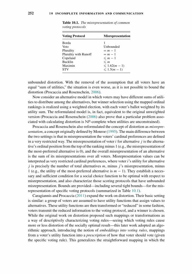
252 1 0 incomplete information and communication
Table 10.1. The misrepresentation of commonvoting protocols
Voting Protocol Misrepresentation
Borda 1Veto UnboundedPlurality = m − 1Plurality with Runoff = m − 1Copeland � m − 1Bucklin � mMaximin � 1.62(m − 1)STV � 1.5(m − 1)
unbounded distortion. With the removal of the assumption that all voters have anequal “sum of utilities,” the situation is even worse, as it is not possible to bound thedistortion (Procaccia and Rosenschein, 2006).
Now consider an alternative model in which voters may have different sums of utili-ties to distribute among the alternatives, but winner selection using the mapped ordinalrankings is realized using a weighted election, with each voter’s ballot weighted by itsutility sum. The reformulated model is, in fact, equivalent to the original unweightedversion (Procaccia and Rosenschein (2006) also prove that a particular problem asso-ciated with calculating distortion is NP-complete when utilities are unconstrained).
Procaccia and Rosenschein also reformulated the concept of distortion as misrepre-sentation, a concept originally defined by Monroe (1995). The main difference betweenthe two settings is that in misrepresentation the voters’ cardinal preferences are definedin a very restricted way. The misrepresentation of voter i for alternative j is the alterna-tive’s ordinal position from the top of the ranking minus 1 (e.g., the misrepresentation ofthe most-preferred alternative is 0), and the overall misrepresentation of an alternativeis the sum of its misrepresentations over all voters. Misrepresentation values can beinterpreted as very restricted cardinal preferences, where voter i’s utility for alternativej is precisely the number of total alternatives m, minus j ’s misrepresentation, minus1 (e.g., the utility of the most-preferred alternative is m − 1). They establish a neces-sary and sufficient condition for a social choice function to be optimal with respect tomisrepresentation, and also characterize those scoring protocols that have unboundedmisrepresentation. Bounds are provided—including several tight bounds—for the mis-representation of specific voting protocols (summarized in Table 10.1).
Caragiannis and Procaccia (2011) expand the work on distortion. Their basic settingis similar: a group of voters are assumed to have utility functions that assign values toalternatives. These utility functions are then transformed or “reduced” in some fashion,voters transmit the reduced information to the voting protocol, and a winner is chosen.While the original work on distortion proposed such mappings or transformations asa way of descriptively characterizing voting rules—seeing which voting rules causemore or less distortion of the socially optimal result—this later work adopted an algo-rithmic approach, introducing the notion of embeddings into voting rules, mappingsfrom a voter’s utility function into a prescription of how that voter should vote (giventhe specific voting rule). This generalizes the straightforward mapping in which the

1 0 .8 social choice from a utilitarian perspective 253
alternative with the kth highest utility is ranked in the kth position; but more funda-mentally, it takes a different perspective on distortion. Instead of using the distortionof specific voting rules as a criterion for evaluating and comparing them, Caragiannisand Procaccia attempt to design embeddings that minimize distortion.
More specifically, one can generalize the notion of distortion, by defining it for gen-eral embeddings. The distortion of a deterministic embedding into a specific voting rulecan be defined, as earlier, as the worst-case ratio of the most popular alternative’s socialwelfare, and the least popular winner’s social welfare. In the case of randomized embed-dings, distortion can be defined using the expected minimum social welfare among thewinners, again looking at the worst-case ratio between the most popular alternative’ssocial welfare, and the expected minimum social welfare among the winners.
Consider the distortion of embeddings into the plurality, approval, and veto votingrules. All of these voting rules have low communication overhead: log(m) bits pervoter for plurality and veto, and m bits per voter for approval, where m is the numberof alternatives. Any deterministic embedding into the plurality voting rule (when n �m) has distortion �(m2). A simple randomized embedding into plurality—where thevoter selects an alternative with probability proportional to its utility—gives constantdistortion when the number of voters n is equal to �(m log(m)), and even for largervalues of n has extremely low distortion, specifically, 1 + o(1). With approval voting,where n � m, there is a lower bound of �(m) for deterministic embeddings. Herethe randomized upper bounds for plurality imply the randomized upper bounds forapproval (since an embedding into plurality is also an embedding into approval).Caragiannis and Procaccia (2011) carry out simulations for the case where n � m,with results supporting the conclusion that low distortion can be achieved if n isnot too small. They also show that any deterministic embedding into the veto rulehas infinite distortion, as is also the case for randomized embeddings if n < m − 1.However, when there are many voters, low-distortion embeddings into veto can beachieved.
The work of Boutilier et al. (2012) is strongly related to the distortion analysisdescribed previously. Taking a utilitarian perspective on social choice, two separatedistortion models are examined, each with a different assumption about the informationthat is available, and each with its own optimality criterion. The first model assumesthat there is no information about voter utility functions, and considers the worst-case optimal social choice function that minimizes distortion on every preferenceprofile; upper and lower bounds are proven on the minimal possible distortion, givenrandomized social choice functions. There exists a preference profile where everyrandomized social choice function has distortion at least �(
√m), where m is the number
of alternatives, and there is a randomized social choice function whose distortion onevery preference profile is O(
√m · log∗(m)). The worst-case optimal social choice
function can be computed in polynomial time.Assume that for each agent i, the sum of the agent’s utilities over all alternatives
a in A is 1. Let R(A) be the set of permutations on [m]. Formally, we have thefollowing theorem (from Boutilier et al., 2012): Assume that n � √
m. Then thereexists a preference profile R ∈ R(A)n such that for any randomized social choicefunction f , dist(f, R) = �(
√m).
254 1 0 incomplete information and communication
Proof. For ease of exposition assume that√
m divides n. Partition the agents into√
m
equal subsets N1, . . . , N√m. Consider the preference profile R where σi(ak) = 1, for
all i ∈ Nk , and the remaining alternatives are ranked arbitrarily.For any randomized f there must be a k∗ ∈ {1, . . . ,
√m} such that Pr[f (R) =
ak∗] � 1√m
. Let u be a utility profile such that for all i ∈ Nk∗ , the value of ak∗ is 1, andthe value of all alternatives other than ak∗ is 0. For all i �∈ Nk∗ and alternatives a ∈ A,the value for i of a is 1
m. It holds that
n√m
� sw(ak∗, u) � 2n√m
,
and for all a ∈ A \ {ak∗ }, sw(a, u) � nm
. Therefore:
dist(f, R) �n√m
1√m· 2n√
m+
√m−1√m
· nm
�√
m
3.
In a second, average-case model, there is a (known) distribution D over voterutility functions. The average-case optimal social choice function is defined as onethat chooses an alternative that maximizes expected social welfare, given a profileproduced by drawing each voter’s utility function independently from D. When D issymmetric with respect to alternatives, this average-case optimal social choice functionmust be a scoring rule (Boutilier et al., 2012).
The focus of Boutilier et al. (2012) on randomized social choice functions differ-entiates their work from that of Procaccia and Rosenschein (2006), which deals withdeterministic social choice functions. Although Caragiannis and Procaccia (2011) alsoconsider randomized social choice functions, their motivations and hence the modelsand assumptions are different. Caragiannis and Procaccia cite communication limi-tations as a primary motivation for voting using rankings (rather than transmittingutility functions). As a consequence, they focus on social choice functions with lowcommunication requirements, with the primary goal being to optimize the embeddingof cardinal preferences into ordinal votes. Boutilier et al. (2012) assume that voterstranslate utility functions into preference orders in the straightforward way (i.e., thealternative with kth-highest utility mapped to the kth position in the vote), and there-fore focus on optimization of the social choice function rather than the embeddingfunction.
10.8.2 Learnability
Consider the scenario where there is a designer who is able, for each input of voterpreferences, to designate a winner. This black box approach assumes that the designer is,perhaps, applying a set of external properties to determine the winner, so that for everyvote profile a winner that satisfies those properties can be specified by the designer. It isassumed that the voting rule that (implicitly or explicitly) drives the choice of winnersby the designer comes from a family R of rules. Procaccia et al. (2009) address theproblem of finding, via some probably approximately correct (PAC) learning process, a

1 0 .8 social choice from a utilitarian perspective 255
voting rule fromR that is as close as possible to the designer’s (implicit or explicit) rule.Ideally, the number of sampled profiles given to the designer should be small (perhapsbecause of the computational or communication costs associated with the process). Analgorithm is developed whose input is a collection of “vote profile-winning alternative”pairs drawn according to the fixed distribution D over profiles. The output is a votingrule that maximizes expected agreement (expectation taken w.r.t. D) between theoutput voting rule and the actual rule from which the samples are derived, in the PACsense.
One way of conceptualizing this problem is as the “automated design of votingrules”; if there exists a specification of properties that can be used to determine a winner,then the process can find a voting rule that in some sense embodies or operationalizesthose properties. The scenario is particularly compelling if there does exist a prior setof criteria for establishing who the winner is, given voter preferences, but no succinctvoting rule that is known to capture those criteria.
There are several interesting results in this model (Procaccia et al., 2009). Given aset of examples, it is possible to efficiently compute a scoring rule consistent with theexamples (if one exists). That, together with the proven dimensionality of the class ofscoring rules (given m alternatives, that dimensionality is bounded by m and m − 3),implies that the class of scoring rules with m alternatives and n voters is learnable inpolynomial time for all m and n.
The situation when R is the family of voting trees is somewhat more complicated;the number of different pairwise voting rules that can be represented as voting trees isdoubly exponential in the number of alternatives. In general, a large number of exampleswould need to be provided to allow learning—this is true even in the seemingly simplercase of balanced voting trees, to which arbitrary unbalanced trees can be transformed.In the special case of “small” voting trees (where the number of leaves in the treeis polynomial in the number of alternatives, rather than exponential in the numberof alternatives), however, voting trees are efficiently learnable. Extensions to generalvoting rules can also be considered, but there exist many voting rules that cannotbe approximated by scoring rules nor by small voting trees (assuming a uniformdistribution over voter profiles). This does not preclude the possibility that there existimportant families of general voting rules that can be approximated by scoring rules orsmall voting trees (Procaccia et al., 2009).
Boutilier et al. (2012) extend the work on learnability further, by considering alearning-theoretic model that is consistent with their overall examination of optimalsocial choice functions from a utilitarian perspective. They assume one has access onlyto sampled utility profiles from some unknown distribution D, and wishes to find asample-optimal social choice function, relative to those sampled profiles (in contrastto the worst-case optimal and average-case optimal social choice functions consideredearlier). The quality of the sample-optimal social choice function is then assessedrelative to the expected social welfare of the (unknown) true optimal social choicefunction for D. Necessary and sufficient bounds are derived on the number of samplesneeded to ensure the sample-optimal social choice function has expected social welfareclose to that of the optimal function with high probability. These are provided forboth k-approval social choice functions, as well as general scoring functions. Finding
256 1 0 incomplete information and communication
the sample-optimal scoring function is APX-hard; however, there is a mixed-integerprogramming formulation that generally enables reasonably effective computation ofthe sample-optimal function.
10.9 Conclusions and Future Directions
We have seen that a number of interesting and challenging issues arise when we considerthe implementation of voting schemes with incomplete information, both conceptu-ally and computationally. At the same time, resolution of these issues allows one todesign mechanisms for preference aggregation that have less stringent informationalrequirements, are more robust with respect to missing information, and minimize thecognitive and communication burden on voters.
We have focused on a few select topics related to voting and partial information.Many interesting avenues are uncovered in this chapter, indeed, several important topicshave yet to be addressed in the literature. We list a few here:
� Manipulation, strategic voting, and equilibrium analysis: Manipulation and control ofelections—and more generally the strategic revelation of preferences—is a topic ofgreat importance (see Chapter 6 and Chapter 7), but much of this work assumes thatmanipulators have full knowledge of the vote profile. Equilibrium analysis of variousvoting rules (Majumdar and Sen, 2004; Angel Ballester and Rey-Biel, 2009) usuallyassumes (more realistically) that voters have incomplete knowledge in the form of acommon prior. Algorithmic and computational study of the complexity and impact ofmanipulation under more realistic incomplete knowledge assumptions has been sparse,but is clearly of vital importance. See Conitzer et al. (2011a) and Lu et al. (2012) forsome steps in this direction. At the same time, many of the models discussed in thischapter—those for vote elicitation, dealing with uncertain alternatives, and learningvoting rules in particular—bring with them new opportunities for vote manipulationand control which require novel forms of analysis. Equilibrium analysis for these newmodels is also required (e.g., see the work of Dutta et al. (2001); Lang et al. (2013),who provide an equilibrium analysis of candidates who choose to enter or abstain froman election).
� Combinatorial domains: Effective means for voting in combinatorial domains is clearlyvital to the practical deployment of the sophisticated preference aggregation mechanisms(see Chapter 9). We have left unaddressed issues associated with incomplete informationin such settings. Incremental vote elicitation schemes for combinatorial domains havebeen few (though see Chapter 9 for discussion of sequential voting mechanisms usingcombinatorial representations). Preference elicitation schemes in nonvoting contextshave been developed for multiattribute preference representations such as CP-networksand soft constraint formalisms (Koriche and Zanuttini, 2010; Dimopoulos et al., 2009;Gelain et al., 2010), and these could be adapted to vote elicitation. However, many ofthe other topics touched on in this chapter have not been addressed in combinatorialsettings.
� Other forms of social choice: Our focus in this chapter has been on social choice inthe “voting” sense. Of course, a variety of other social choice problems are amenable
1 0 .9 conclusions and future directions 257
to the same types of partial information analysis discussed here, including two-sidedmatching (Chapter 14), coalitional matching and group formation (Chapter 15), assign-ment problems, multiwinner (or committee) voting problems (Chapter 9), fair division(Chapters 11–13) among others. For example, communication complexity, matchingwith incomplete information, and incremental preference elicitation have begun to gar-ner attention in the stable matching domain (Chou and Lu, 2010; Pini et al., 2011b;Drummond and Boutilier, 2013; Rastegari et al., 2013; Liu et al., 2012).


PART II
Fair Allocation

CHAPTER 11
Introduction to the Theory ofFair Allocation
William Thomson
11.1 Introduction
The purpose of this chapter is to briefly introduce the theory of fair allocation in thecontext of concretely specified economic environments. There, requirements of fairnessare expressed in terms of resources and opportunities understood in their physical sense.Thus, it contrasts with abstract social choice theory as this expression is commonlyunderstood: in the canonical Arrovian model (Part I), the alternatives available to societyare not structured in any particular way, whereas in models of resource allocation, thespace of feasible alternatives is equipped with a variety of mathematical structures,topological, vectorial, and order structures. This enrichment has implications on severallevels. First, when we specify the model itself, we can include properties of preferencesreflecting these structures that would not be meaningful without them. Second, we canformulate properties of allocation rules referring to the structures. Finally, we candefine allocation rules that are based on the structures.
Abstract social choice theory and the theory of fair allocation have the same con-structive objective, however, namely, to identify the “best” way of reconciling theconflicting interests of the participants. In each case, we can distinguish two branchesof the literature. The normative branch focuses on the distribution of welfare throughoutthe population. It starts with the formulation of criteria of fairness, and it studies theirimplications. The strategic branch is concerned with the fact that agents have somecontrol over resources, technologies, and the information about the outside world ortheir own preferences, and that they may try to take advantage of this control. Ideally,the allocation process should be safe from manipulation of resources or technologies,by individual or by groups, and from misrepresentation of their knowledge of the envi-ronment or of their preferences. We focus on the normative branch here but there isnot a complete conceptual separation between normative and strategic considerations;some properties of rules can be interpreted from either viewpoint; also, from a technicalperspective, the two branches are linked in multiple ways.
The primary aim of abstract social choice theory is to define social orderings over theset of alternatives, whereas most of the theory we review here deals with how to choose,
261

262 1 1 introduction to the theory of fair allocation
for each economy, one (or several) allocation(s) from a set. These allocations can ofcourse be understood as maximizing an implicit social ordering (the two-indifference-class ordering in which the higher indifference class consists of the allocations thatare chosen, and the lower one consists of the allocations that are not chosen), but noattempt is made at elucidating these orderings themselves, and in particular, at derivingfine orderings from desirable properties of the process of preference aggregation. Foran up-to-date treatment and new perspectives on such derivations, see Fleurbaey andManiquet (2011).
Given the space constraints we face, we are unable to give extensive referencesto primary sources and instead, we refer to surveys. They concern either a specificprinciple or a particular type of allocation problems. General references are Young(1995b), Brams and Taylor (1996), Moulin (1995), Moulin (2004), Barbanel (2005),Thomson (2011), and Thomson (2014d). We focus on the axiomatic approach tofairness. We ignore the experimental literature, how lotteries can be used to achievefairness in the ex ante sense, and strategic issues. Among the multiple types of allocationproblems in which fairness have recently been addressed, we chose some that we feltwere representative of the literature as a whole. A large number of papers focus onthe interaction of normative and strategic requirements, in particular the incentive thatallocation rules provide agents to be truthful about their preferences (Barbera, 2011).We have chosen not to review this literature. Also, several of the chapters in this volumeaddress such issues (Chapters 1, 6, and 14).
Finally, we do not consider computational issues. These are already the centralfocus of many of the other chapters in this volume. It has been very rewarding toeconomists who have been involved in the development of the theory of fairness to seethe increasing interest that the computer science community has taken in the subject.This interest has been uneven, however. The concept of an envy-free allocation, theclassical problem of fair division, the division of a measure space, and various types ofallocation problems with discrete structures, such as object allocation or reallocationproblems and two-sided matching, have indeed received considerable attention in thiscommunity, but there are other facets of the theory, a range of other concepts andother types of allocation problems on which it has not yet brought to bear its ownperspectives and techniques, and we hope that this survey will help further cross-fertilization between computer science and economics. Examples are the punctualnotions of egalitarian-equivalence and of equal opportunities, and the many relationalsolidarity requirements that have been critical in axiomatic analysis. As for types ofallocation problems that would benefit from being more closely examined from thecomputational angle, are problems with satiated preferences, claims problems, costallocation problems (they come in a great variety), and public goods problems. Here isnot the place to be formal; these terms are defined in what follows.
We first describe a generic allocation problem, listing its components. We introduceseveral standard, and some not so standard, classes of allocation problems. Next, weintroduce the principles that constitute the conceptual core of the literature under review.We hope to show that in spite of the great diversity in the axioms that have been studied,they can all be seen as expressions of just a few general principles. However, becauseeach class of problems has its own mathematical structure, these principles often haveto be adapted. Also, the implications of a particular combination of principles often

1 1 .2 what is a resource allocation problem? 263
differ significantly from one class to the other. It is also the case that for some classesof problems, additional concepts may be available that are not meaningful in others.
11.2 What Is a Resource Allocation Problem?
We begin with a presentation of the data needed to specify an allocation problem, andwe continue with a sample of problem types. We chose them to illustrate the scope ofthe program surveyed here.
11.2.1 The Components of an Allocation Problem
An economy has several of the following components:
1. A set of agents: this term may refer to individual people, to government agencies, tofirms, or to other entities, such as “artificial” agents acting on behalf of “real” agents.
2. Resource data concerns unproduced endowments of goods that can be either consumedas such or, when production opportunities are specified, used as input in the productionprocess; in that case, we also specify production sets and we may attach productivityparameters to agents or to groups. From all of the data we derive feasible sets or oppor-tunity sets open to agents or to groups. In general equilibrium theory, a production planis a point in commodity space interpreted as a feasible input-output combination. Someof the inputs may be labor inputs, and because people may be differently productive,productivity parameters may be specified, giving the rate at which each person’s labortime can be converted into abstract labor.
3. Ownership data may concern unproduced resources or production processes. Ownershipmay be individual: a particular agent may own a particular resource, his house, his ownself. It can be semi-collective: a particular group of agents may own a particular resource,for example a married couple may jointly own the house in which they live. It may becollective: the entire agent set may own a particular resource; for example, a nation ownsits cultural patrimony. It may be mixed: some resources may be owned privately; otherresources may be owned by a group of agents; yet others may be owned by the entire agentset; an example here consists of the housing units to which some students are returningat the beginning of the academic year and that they have the right to keep—in a sense,these resources are owned by these students—and the units that have been vacated by thestudents who graduated and left—these constitute a collective endowment. Ownershipmay be contested, disagreement over it resulting in incompatible claims.
4. Priority data indicates the precedence to be given to particular agents over others.Priority can be absolute, as when a linear order is specified on the agent set, no two agentsbeing at the same level. Alternatively, it may be relative, with nontrivial indifferenceclasses. It may be restricted and structured, because of upper bounds on how muchagents are allowed to get. Then, once the highest-priority agent has been given hisassignment—here, it is difficult to describe the data without suggesting how they maybe used—we need to specify who comes next, who comes after this second agent, andso on. The structure may take the form of a limit on the scope of priorities, as whena priority is attached to only some of the resources, or when different priorities are
264 1 1 introduction to the theory of fair allocation
attached to different resources. In any of these situations, giving priority to an agentdoes not mean giving him control over, or access to, every single resource.
5. Preference data concerns natural properties that, for each class of problems underinvestigation, we expect preferences to satisfy; these properties depend in an importantway on the mathematical structure of the set of possible consumptions for an agent, thatis, on the nature of the resources to be assigned. To illustrate, when goods are infinitelydivisible, consumption bundles are vectors in a Euclidean space. This space is equippedwith topological, order, and convex structures, and we can require preferences to satisfycontinuity, monotonicity, and convexity properties. Using the notation a � b to meanthat a is at least as desirable as b, and a � b to mean that a is preferred to b, theseproperties can be written as follows: (i) if xi �i yi , x ′
i is sufficiently close to xi and y ′i
is sufficiently close to yi , then x ′i �i y ′
i ; (ii) if yi � xi , then yi �i xi , and (iii) given anybundle xi , {yi | yi �i xi} is a convex set.
6. Bounds may be imposed on consumptions. They may be lower bounds or upper bounds.We may require a minimal consumption of a particular good (education), or we mayrequire a maximal consumption of a good (only one time slot per person for someactivity).
We will not discuss models that include utility information. We will not attempt tomeasure welfare gains and losses on cardinal scales, let alone compare such quantitiesacross agents. Indeed, an important development of the last decades is that purelyordinal criteria have gained general acceptance. They save us from having to addressthe delicate conceptual and practical issues raised by the use of utilities. Besides, aswe will see, we will have to present a number of negative results and the mild formof our ordinal criteria will make these results all the more striking. When positiveresults emerge, they are often uniqueness results, and in such cases, even if cardinalinformation were available, it would have to be ignored. We do not mean to suggest thatan ordinal approach is superior to a utility based approach, but it is its ordinal characterthat makes the recent literature on fairness particularly noteworthy as compared totraditional welfare economics, and it is the literature that we survey.
Once we have specified all of this data, we have a domain of economies. Ourobjective is not just to make a recommendation for the particular allocation problemthat we happen to face today, but to make a recommendation for each problem in somedomain of interest. This takes us to the concept of a solution or rule (Section 11.3).
11.2.2 A Range of Resource Allocation Problems
Fairness issues have been studied in the context of a great variety of resource allocationproblems. We have chosen several of them to illustrate the central concepts.
1. Classical fair division problems. A social endowment � ∈ R + of infinitely
divisible goods has to be distributed among a group N of agents. Each agent i ∈ N isequipped with a preference relation�i over -dimensional commodity space R
+. Thesepreferences satisfy “classical” assumptions of continuity, monotonicity, and convexity.
2. Fair division problems with single-peaked preferences (Sprumont, 1991). A socialendowment � ∈ R+ of a single commodity has to be fully (there is no possibility ofdisposal) distributed among a group N of agents. Each agent i ∈ N has preferences
1 1 .2 what is a resource allocation problem? 265
�i with the following features: up to some critical level, his peak amount, denotedp(�i), an increase in agent i’s consumption increases his welfare, but beyond thatlevel, the opposite holds: for each pair xi, x
′i such that either x ′
i < xi � p(�i) orp(�i) � xi < x ′
i , we have xi � x ′i . Such preferences are single-peaked. An example is
the parceling out among workers of a task that must be completed, when each worker ispaid a fixed wage and has convex preferences in leisure-income space. Thus, the modeldiffers from the previous one (essentially) in that there is only one commodity here andthe assumption of monotonicity of preferences is dropped; however, the assumption ofconvexity is retained. Violations of monotonicity raise challenging questions even inthe one-commodity case.
3. Claims problems (O’Neill, 1982). A social endowment � ∈ R+ of a single goodhas to be distributed among a group N of agents with incompatible claims on it.Denoting by ci ∈ R+ the claim of agent i ∈ N , incompatibility means that
∑ci > �.
Agents have monotonic preferences. (Thus there is no need to include preferencesexplicitly in the formal description of a problem: there is only one monotone preferencerelation defined over the nonnegative reals.) A typical application is to bankruptcy: theliquidation value of a bankrupt firm does not allow to fully satisfy all of its creditors.Mathematically, the problem of raising taxes from the users of a public project as afunction of their incomes to cover the cost of the project, or as a function of the benefitsthey derive from it, is equivalent. Surveys are Thomson (2003) and Thomson (2014a).A related class of problems are surplus-sharing problems. They differ from claimsproblems in that the endowment exceeds the sum of the claims. It is also meaningfulto jointly study both claims and surplus-sharing problems.
4. Partitioning nonhomogeneous continua. A social endowment consisting of aninfinitely divisible and nonhomogeneous continuum has to be partitioned among agroup N of agents. The dividend is a measure space and each agent i ∈ N has prefer-ences defined over its measurable subsets. In the base model, agent i’s preferences �i
are monotonic with respect to set inclusion (if I ⊃ I ′, then I �i I ′).It is also common to take the dividend to be a subset of a finite-dimensional Euclidean
space and the one-dimensional case is of special interest. Think of an interval oftime I ⊂ R+ during which a service is provided, for example, maintenance or repairwork on a machine, or instruction on how to use it. The value of the service to anagent depends on how long it lasts and when it is provided, and it varies from agentto agent. In many situations, such as the service example just mentioned, it makessense to require that each agent be assigned an interval, but not always, as whenthe issue is to schedule when students in a group will be assigned weekly individualreview or practice sessions with tutors. (Chapter 13 discusses algorithmic issues in thiscontext.)
The one-dimensional continuum may be circular. An example here is a marketaround a lake in a mountain resort that has to be partitioned into intervals to beassigned to ice-cream or souvenir vendors, their potential customers being unevenlydistributed around the lake. A cake on which frosting and decorations are distributedunevenly and that has to be partitioned into slices is another example.
The dividend may be undesirable in the sense that of two intervals related byinclusion, the smaller one is preferred to the larger one. Here, and in the context ofthe tutoring example mentioned previously, think of the teaching assistants who have

266 1 1 introduction to the theory of fair allocation
to staff the office where they will help out students with their homework assignments,and of police patrolling the road around the lake.
As illustrations of the two-dimensional case, consider the problem of partitioningfarmland bequeathed by a farmer to his children, or assigning tracts of land to miningcompanies for gas or oil exploration, or the ocean floor for nations to exploit mineralslying there.
Much of the literature concerns the case of preferences that can be representedby atomless measures. This additivity assumption is restrictive, as it precludes thepossibility that a subset be valuable only if some other subset is consumed with it (thatis, it rules out complementarities), or conversely that a subset not be valuable becausesome other subset is already included in someone’s assignment (the two subsets aresubstitutes then). Additional topological and geometric—we could say “geographic” inthe case of land—criteria are sometimes meaningful. For instance, it may make sense torequire connectedness of each component of the partition, or contiguity of each agent’sassignment to some prespecified endowment that is not part of the redistribution.
5. Object allocation problems. A social endowment O of indivisible goods, orobjects, has to be assigned to a group N of agents. Each agent i ∈ N can consume onlyone and has preferences �i defined over O. The objects are the only resources. This isthe base case of an object allocation problem. Think of offices to assign to the membersof an academic department moving to a new building, or of tasks to be assigned by aforeman to the workers in his team (see also Chapter 12).
More generally, each agent i ∈ N may consume several objects and have preferencesdefined over 2O . Estate or divorce settlements often involve multiple indivisible items(painting, silverware) and each heir will receive several. Selling these resources anddividing the proceeds among the intended recipients may come to mind as a solutionbut this may be very imperfect. Indeed, these resources may have value to them thatare not recognized on the market (family heirlooms), or legal constraints may preventappealing to a market altogether (organs).
The simplest case is when the numbers of objects and agents are equal. When thereare fewer objects than agents, some agents have to go without one. We allow for thispossibility and augment the set of objects by a null object; by definition, there arealways enough copies of it for each agent to receive one (real or null) object. An objectis desirable for an agent if he prefers it to the null object, and undesirable if the oppositeholds. When there are fewer agents than objects, some objects have to be unassigned.In some applications, it is natural to require that the null object not be assigned until allreal objects are, even if these objects are undesirable, or undesirable for some agents.An example here is the problem of assigning household tasks to housemates. Noneof them may enjoy a particular task; yet, the task has to be performed (cleaning, forexample); alternatively, some of them may find a particular task desirable and othersnot (cooking a meal illustrates the possibility).
6. Objects-and-money allocation problems. We enrich the previous model by addinga social endowment of one infinitely divisible good that, with some abuse of language,we call “money.” Each agent i ∈ N can consume some amount of money and oneobject. Consumptions of money may be unrestricted in sign, or they may be required tomeet a lower bound (for example zero). Thus, each agent has preferences defined overthe cross-product R × O, perhaps [a,∞[×O for some a ∈ R. They are continuous,

1 1 .2 what is a resource allocation problem? 267
strictly monotonic with respect to money, and such that, starting from any bundle,replacing the object it contains by any other object can always be compensated by anappropriate change in the consumption of money. Here too, the base situation is whenthe numbers of objects and agents are equal. An example is the problem of assigningstudents to rooms in the house they are renting together, and specifying for each ofthem his share of the rent.
As in plain object-allocation problems, when there are fewer objects than agents,some agents have to go without one. As before, we then augment the set of objects by anull object. In the room-assignment–and–rent-division example, the null object can beinterpreted as “looking for other accommodation.” When the null object is available,we say that a real object is “desirable” for an agent if, given any bundle that includes it(that is, no matter how much of the divisible good is consumed with it), replacing it bythe null object leads to a bundle that is at most as desirable. An object is “undesirable”if the opposite always holds.
7. Priority-augmented object allocation problems (Balinski and Sonmez, 1999;Abdulkadiroglu and Sonmez, 2003). Here, we enrich the object allocation problem ina different way, by imagining that each object a ∈ O is equipped with a priority orderπa over its possible recipients. An example is “school choice”: the objects are seats inschools; at each school, a priority order over students is given (the order may dependon several factors: whether a student already has a sibling in the school; whether helives in the “walk-zone” of the school; how long he has been on the waiting list; hisacademic record; and so on). At each school a ∈ O, a capacity κa is specified. In thatapplication, indifference has to be allowed: two seats at a given school have to beconsidered equivalent by a student, but indifference is very structured in the sense thatany two students are indifferent between all the seats at each school. (For a survey, seeAbdulkadiroglu (2013).)
8. Matching agents to each other. Now, we a priori partition the agent set into twosets. Each agent has preferences over the agents in the component of the partition towhich he does not belong. The objective is to make pairs containing one agent fromeach set. There is a wide variety of matching models, however: (i) the option of notbeing matched may be present or not; (ii) in the base model, matching is one-to-one,an example here is when men and women have to be paired for a dance class, or whenmedical students have to be matched to hospital programs for residency; matchingmay also be several-to-one, an example being when high-school graduates have tobe assigned to colleges; several-to-several matching are possible in some situations,an application here being when a worker can work for several firms and a firm canemploy several workers; (iii) preferences may be strict or indifference may be allowed;(iv) there may also be some amount of an infinitely divisible good, typically money,to distribute, and here, how much of it there is may be derived from the pairs that areformed. There, agents may only care about how much of the divisible resource theyare assigned, not about to whom they are paired, or they may care about both. Anapplication here is the assignment of workers to firms, when each pair of a worker anda firm is worth so many dollars (or when each pair consisting of a set of workers anda firm is worth so many dollars), and the amount to divide is the sum of the worthsgenerated by all the pairs that are created. In the simplest case, illustrated by the men-women metaphor, N = M ∪ W , each i ∈ M has preferences over W and each i ∈ W

268 1 1 introduction to the theory of fair allocation
has preferences over M . For the problem of pairing workers and firms, to each pair(w, f ) is associated a number a(w, f ), and the amount to divide is
∑a(w, f ) over all
pairs (w, f ) that are formed. An introduction to the literature is Roth and Sotomayor(1990) (also see Chapter 14). Related to two-sided pairing problems are roommateproblems, which are one-to-one pairing problems in which each agent can be matchedto any other agent. The theory of coalition formation is a generalization. There, theagent set has to be partitioned into subsets, taking the preferences of each agent overall subsets into account.
Listing the components of an allocation problem in the manner we did earlier raises anumber of questions. What does it mean to say that a resource is a “social endowment,”that an agent “owns” a resource, that a priority order on the possible recipients isattached to a resource, that a priority order on the possible recipients is attached toeach of several resources? What is the operational meaning of these expressions? Howshould they be reflected in properties of allocation mappings?
11.3 Solutions and Rules
A solution associates with each problem in the class under investigation a non-emptysubset of its set of feasible allocations. A rule is a single-valued solution. Thus,a rule provides a complete answer to the question of how to allocate resources ineach particular problem in the class under investigation. A solution only achieves afirst-round elimination of alternatives, the process through which a final outcome isdetermined being left unspecified.
We can arrive at solutions and rules in a variety of ways.(i) A solution may formally describe what we observe in actual practice. It is impor-
tant to understand what is done in the real world, to know the desirable features aswell as the undesirable features of common practices. Societies have occasionally hitupon attractive procedures to resolve conflicts over allocation of resources, and we maybe able to draw useful lessons from scrutinizing these procedures. Examples are rulesbased on equality, proportionality, priority, lotteries, and prices. Of course, for this exer-cise to be meaningful, we have to formulate criteria of desirability. We turn to them next.
(ii) The core of the second approach are principles of good behavior of solutions orrules. An “axiom” is the mathematical expression of some intuition we have about howa solution or rule should behave in certain situations. An axiomatic study starts with alist of axioms and its goal is to describe the implications of the axioms when imposedin various combinations. The ultimate goal of the axiomatic program is to trace out theboundary that separates those combinations of axioms that are compatible from thosethat are not. (Chapter 2 is an example of a chapter that is mainly axiomatic, but axiomsare discussed throughout the book.)
The scope of certain principles is very broad, that is, these principles can be mean-ingfully expressed in almost any model. An example is the economist’s central notionof “Pareto-efficiency”: an allocation x is efficient (for short) for some economy if thereis no other allocation x ′ that all agents find at least as desirable and at least one agentprefers, that is, such that for each i ∈ N , x ′
i �i xi and for some j ∈ N , x ′j � xj . Other
1 1 .3 solutions and rules 269
principles, although not totally model-free, still have a broad range of applicability.An example is the no-envy notion (Foley, 1967),1 according to which no agent preferssomeone else’s assignment to his own: there is no pair i, j ∈ N such that xj �i xi .The permutations on which it is based presume that all agents’ preferences are definedover the same space, and that if agents differ in some relevant dimension other thanpreferences, some adjustments can be made to place them on the same footing. Forinstance, when the issue is to reallocate bundles that agents privately own, and callingωi and ωj agent i and j ’s endowments, we can adapt it by requiring that there is nopair i, j ∈ N such that [ωi + (xj − ωj )] �i xi . This is the notion of no-envy in trades(Kolm, 1972; Schmeidler and Vind, 1972). The no-envy notion makes the most sensewhen applied to the distribution or redistribution of private resources. It is silent inmodels of “pure” public choice, where by definition, all agents consume the samething and a compromise has to be found on what that common assignment should bebecause agents differ in how they value it.
Other principles may be applicable in several contexts but in each particular one,some adaptation is needed, and various expressions of the idea may be meaningful.Monotonicity requirements come to mind here and we will give several examples toillustrate the point.
Some of the principles directly define solutions and rules, and others only placeconstraints on how the choice of an allocation may vary in response to changes in thedata of a problem. For instance, efficient allocations exist almost always. Thus, wecan speak of the solution that selects for each economy its set of efficient allocations.By contrast, the self-explanatory requirement of equal treatment of equals does notsuggest the definition of a solution, because there are many economies in which notwo agents have the same characteristics. And even if some agents do have the samecharacteristics, what should their common consumption be and what are we supposedto assign to the others?
(iii) The well-developed theory of cooperative games is also a good source ofinspiration for solution concepts and principles. However, the models that are studiedin that theory are “abstract” in the sense that only sets of achievable utility vectors aregiven. The description of the actual physical choices that agents have is typically notincluded in their specification. By contrast, we are interested here in settling concretelyspecified resource allocation problems. Part of the conceptual work to undertake whenexploiting the theory of cooperative games is to find the most natural expressions inthe context of the model under study of the principles that have been important inthat theory. Alternatively, we can map the allocation problems under investigation intogames and apply solutions introduced in the theory of games to solve these games. Aresource allocation problem can often be mapped into a game in more than one way,however (the result may be a bargaining problem, a transferable utility game, or anontransferable utility game), and proceeding in this way will give us the opportunityto apply different solution concepts of game theory to solve our allocation problem.
(iv) Rules that are common in one area may serve as a source of inspiration indefining new rules in other areas. For example, for the standard model of general
1 This notion is also called “envy-freeness.”
270 1 1 introduction to the theory of fair allocation
equilibrium, in which agents may have different endowments, the central rule is theWalrasian rule: given some prices p in the simplex of R
+, we let each agent i maximizehis preferences �i in his budget set (the set of bundles xi whose value pxi does notexceed the value pωi of his endowment ωi), and adjust prices so as to obtain equality ofdemand and supply:
∑x∗
i = ∑xi , where x∗
i designates agent i’s maximizing bundle.2
To solve classical fair division problems, we operate this rule from equal division, thatis, we endow each agent with an equal share �
|N | of the social endowment. We therebyobtain the equal-division Walrasian rule, the rule that comes to the minds of mosteconomists first. It has the merit of offering to all agents the same opportunities, theseopportunities being defined through prices. For single-peaked allocation problems, theuniform rule U can also be seen in the light of equal opportunities (Sprumont, 1991).“Budget sets” here are intervals from the origin to some upper bound if the sum ofthe peak amounts exceeds the social endowment, and from some lower bound to thesocial endowment otherwise: given e ≡ (�,�) ∈ EN
sp, if∑
p(�i) � �, then for someλ ∈ R+ and for each i ∈ N , Ui(e) = min{p(�i), λ}; if
∑p(�i) � �, then for some
λ ∈ R+ and for each i ∈ N , Ui(e) = max{p(�i), λ};For priority-augmented object allocation problems, the theory of two-sided matching
has been important in defining solutions. Prominent rules are the immediate acceptancerule, according to which we identify the various agents’ most preferred objects andwe assign each object to the agents listing it first, in the order of their priority for thatobject, until its supply is exhausted; we reject the others; at the next round, each rejectedagent “applies” to his second most preferred object. We repeat the operation with them,after adjusting the supplies of the objects down by the number of times it has beenassigned at the first round. We proceed until each agent has been assigned an object. Forthe tentative acceptance rule3 (Chapter 14), at each round we only tentatively assignobjects and keep as potential assignees of each object those recipients who have thehighest priority among those we kept on as potential assignees at the previous roundand the agents who are newly requesting it. As for the immediate acceptance rule, eachagent whom we reject at some round applies to his next most preferred object at thenext round. The algorithms stop when no one is rejected.
11.3.1 Axioms
Our goal here is not just to try to understand the implications of fairness requirementsfor allocation rules; we have to define fairness to begin with. Perhaps we should beginby requiring that all agents should be treated equally, that they should be put “onthe same level.” The objective of treating all “equal” agents “equally” seems ratherlimited if by “equal” agents we mean agents that nothing distinguishes in their formaldescriptions. Indeed, it would not cover many situations. Because in discrete allocationproblems, there are finitely many possible preferences, it is applicable to a positivefraction of all preference profiles but otherwise, there may be few agents with the same
2 A pair (p, x) as just described is often called an “equal-income competitive equilibrium,” and the allocationx an “equal-income equilibrium allocation.” The mapping that associates with each economy its equilibriumallocations is also known as the “equal-income competitive equilibrium correspondence.”
3 Commonly known as the “deferred acceptance rule.”
1 1 .3 solutions and rules 271
characteristics, or none. Besides, it will not be enough: equal assignments may notbe compatible with efficiency. They may not even exist. Again, an example here is,when the resources to allocate present indivisibilities. In an object allocation problemin which all agents have the same preferences, it obviously cannot be met.
The real challenge is to recognize differences between agents when they exist, andto treat these differences appropriately. What should we do when two agents havedifferent preferences? When they have contributed differently to the production of theresources available for distribution, either in labor time, or because they are differentlyproductive, or both? When they differ which respect to claims they have, resources theycontrol, or characteristics that are not related to economic activities, such as record ofservice or medical condition?
Recognizing departures from fairness, measuring them, assessing their significance,and perhaps redressing them, is also part of the study of fairness. Developing menus ofparameterized rules from which the user of the theory can choose so as to best fit hisneed for a differential treatment of different agents is another objective of the theoryof fairness.
11.3.2 Punctual Axioms
We can distinguish between different types of requirements on solutions and rules. Webegin with punctual requirements, that is, requirements that apply to each economyseparately, “point by point.” The question to be addressed then concerns the existence,for each economy in the domain under consideration, of allocations satisfying theaxiom. When a punctual axiom meaningfully restricts the set of possible allocations ofeach economy—we could say that it has full coverage then—it defines a solution or arule. Here are the central ideas.4
(i) Bounds on physical assignments or on welfares can be defined agent by agent,in an “intra-personal” way. They are usually lower bounds, offering each agent aguarantee that at the allocation chosen by a rule, his welfare will be above a certainlevel, defined in terms of the social endowment and his preferences. Others are upperbounds, specifying for each agent a ceiling on his welfare. Imposing such a ceiling canbe seen as another way of preventing the others from being unduly burdened by hispresence.
To illustrate, for classical fair division problems, an allocation satisfies no-domination of, or by, equal division, if (i) no agent is assigned at least as muchas an equal share of the social endowment of each good and more than an equal shareof the social endowment of at least one good, or (ii) at most as much as an equalshare of the social endowment of each good and less than an equal share of the socialendowment of at least one good, that is, there is no i ∈ N such that either xi � �
|N | or
xi � �|N | .
The notion just defined is preference-free, by contrast with the next ones. An allo-cation x satisfies the equal-division lower bound if each agent finds his assignment at
4 In social choice theory (Part I), the distinction is often made between intra-profile axioms and inter-profileaxioms, but we prefer avoiding this language because a relational axiom may have to do with a change in asingle parameter, not a change in a profile of parameters.
272 1 1 introduction to the theory of fair allocation
least as desirable as equal division: for each i ∈ N , xi � �|N | (among many others,
Kolm, 1972; Pazner, 1977).5
Having all agents share the benefit, or the burden, of their diversity is another impor-tant idea. If one had the choice of joining an economy in which agents have differentpreferences from one’s own or joining one in which they have similar preferences,which decision should one make? Of course, it depends on how the resources wouldbe allocated but in an economy of clones, efficiency and the minimal requirement ofequal treatment of equals together usually determine the allocation. It also depends onthe nature of the goods and, when they have to be produced, on the properties of thetechnologies under which they are produced. Let us answer the question in the contextof some of our models.
In a classical fair division problem, diversity is a good thing. When agents havethe same convex preferences, equal division is efficient. Introducing diversity allowsdistributions that all agents prefer to equal division, and ensuring that all agents benefitfrom their diversity is a meaningful objective. One way to implement it is as follows:for each agent, imagine the hypothetical situation in which everyone else would havehis preferences. Then, if preferences are convex, under efficiency and equal treatmentof equals, the common welfare of these clones would be what they experience at equaldivision. Returning to the actual economy, sharing the benefits of diversity would betranslated into the requirement that each agent’s welfare level at his assignment be atleast as high as the common welfare level that he and his clones would experience inthis counterfactual economy. This is simply the equal-division lower bound. In othermodels, the reference to economies of clones has led to new lower bounds, however.
In other situations, diversity is a burden. When it comes to the production of privategoods under increasing returns-to-scale, or the production of public goods, similarityof preferences is preferable.
In yet others, diversity may be a good thing or a bad thing depending upon particularfeatures of the economy, and we can refer to economies of clones to define a boundthat is a lower bound or an upper bound.
(ii) Requirements based on inter-personal comparisons of assignments, or moregenerally, “opportunities” can also be defined. We can base these comparisons onexchanges of these objects, or perhaps on other operations performed on them.
Recall the definition of an envy-free allocation. The no-envy notion can be adapted toassess the relative treatment of groups of agents too: an allocation x is group envy-freeif given any two groups of the same size, G and G′, we cannot redistribute among themembers of G what has been assigned in total to the members of G′, namely,
∑G′ xi ,
so as to make each member of G at least as well off as he was at x, and at least one ofthem better off. We can adapt the definition to accommodate groups of different sizes,by performing calculations on a per capita basis, that is, by making available to G thebundle |N |
|N ′|∑
G′ xi .The next definition is based on evaluating an allocation by comparison to a counter-
factual allocation at which all agents would receive the same bundle: equivalently, theallocation x is egalitarian-equivalent if there is a “reference” bundle x0 that each agent
5 This requirement is usually called “individual rationality from equal division.”
1 1 .3 solutions and rules 273
finds indifferent to his assignment: for each i ∈ N , xi ∼i x0 (Pazner and Schmeidler,1978). Then, the “obvious” fairness of a hypothetical allocation composed of multiplecopies of the same bundle x0—hypothetical because this list of identical bundles isnot usually feasible—is transferred to the allocation x that is being evaluated throughPareto indifference. The definition is not very restrictive; in fact, one can argue that it istoo permissive. For instance in the context of classical fair division problems, it is easyto construct examples in which some agent is assigned a share of the resources that isarbitrarily close to one. However, for this model, we can define various selections fromthis correspondence that have considerable interest. Fix a direction r in commodityspace. An allocation x is r-egalitarian-equivalent if there is λ ∈ R+ such that for eachi ∈ N , xi ∼i λr . When r = �, the resulting rule is particularly attractive. For example,it also meets the equal-division lower bound.
More generally, we may require the reference bundle to belong to some path G incommodity space that emanates from the origin, is monotone and whose projection oneach axis is unbounded. Then, x is G-egalitarian-equivalent if there is x0 ∈ G such thatfor each i ∈ N , xi ∼i x0. The considerations underlying the no-envy and egalitarian-equivalence criteria (and variants) seem to be far removed from each other but in fact,they can be seen as special cases of a general definition (Thomson, 1994b). We canconstruct for each agent i ∈ N , a representation of his preferences by “calibratingon G” as follows: to each bundle x0 ∈ R
+, declare the agent’s welfare to be equal tothe length of the part of G that extends from the origin to the point of G that he findsindifferent to x0. Then, a G-egalitarian-equivalent allocation can be described as oneat which all agents experience the same welfare. Note that the definition is entirelyordinal; it involves no utility considerations.
The success of the no-envy notion comes in part from the fact that it is well-defined in models in which equal division, and comparisons to equal division, are notmeaningful or possible: they pertain to object allocation, object-and-money allocation,priority-augmented object-allocation, one-to-one matching, and the partitioning ofnonhomogenous continua. The same comment applies to egalitarian-equivalence andsome of its variants. Now, to say that a concept is meaningful is not to say thatallocations satisfying it necessarily exist. In fact, we will see that discreteness of anallocation space raises serious existence problems.
The requirements discussed so far are most meaningful when ownership of resourcesis collective, but they can sometimes be adapted so as to take account of privateownership. This is particularly so in the context of classical fair division problems,because one can measure the vectorial difference between an agent’s assignment andhis endowment, and compare these differences across agents. For instance, the no-envynotion can be applied to trades, as we have seen. For object allocation problems forexample, such tests are not meaningful.
11.3.3 Relational Requirements
A relational requirement prescribes how a rule should respond to changes in someparameter(s) of the economy. The most central notion here is that of solidarity: ifthe environment in which a group of agents find themselves changes, and if no onein this group is responsible for the change, that is, if no one deserves any credit or
274 1 1 introduction to the theory of fair allocation
blame for it, the welfare of all of these agents should be affected in the same direction:either they should all be made at least as well off as they were made initially, or theyshould all be made at most as well off. The terms “credit” and “blame” suggest thatthe change is good and bad respectively, but in what sense? One possibility is that itcauses an expansion of opportunities in the first case and a shrinking of opportunitiesin the second case. A narrower meaning is when the change is evaluated in relation tothe choice made by the rule initially. In the first case, the change is good if a Paretoimprovement over that initial choice is possible; in the second case, when it is not, theinitially chosen profile of welfares is not feasible anymore.
In applications, the parameter often belongs to a space equipped with an orderstructure. Then, we can speak of the parameter being given a “greater” or “smaller”value in that order. Then, together with efficiency, and given the assumptions madeon preferences, the solidarity requirement often implies a specific direction in whichwelfares be affected. We require then that when a Pareto improvement is possible, allagents be made at least as well off as they were made initially; otherwise, that theyshould all be made at most as well off. In such cases, solidarity takes the form of a“monotonicity” requirement.
Note, however, that efficiency considerations come into the picture here. Solidarityin its “pure” form simply says that when a change in the environment of a group ofagents occurs for which none of them bears any particular responsibility, the welfaresof all of its members should move in the same direction. Making all agents worseoff when opportunities expand could only be described as a perverse application ofthe idea, but it is important to see that insisting on a weak improvement for everyonehas to implicate more than solidarity considerations. It does not imply the full force ofefficiency because an inefficient choice could of course be followed, after opportunitieshave expanded, by a Pareto-dominating choice that is also inefficient.
In some models, the general idea may be given several expressions, expressionsthat are based on the data of the problem. For example, when applied to object-and-money allocation problems, two requirements can be expressed, first a requirement ofmonotonicity with respect to expansions of the object set and second, a requirementof monotonicity with respect to the amount of money available. In the context ofsingle-peaked allocation problems, the structure of the situation gives us no choice butto consider the general expression of the solidarity idea, not its “efficiency-inclusive”monotonicity expression. It simply says that any change in the endowment shouldaffect the welfares of all agents in the same direction.
The parameter that varies may not belong to a space that is equipped with an orderstructure. Then, whether a change in its value is beneficial to society or not depends onthe other parameters of the problem. The requirement of solidarity retains its generalform, namely, that all agents be affected in the same direction, but this direction is notspecified.
Finally, even if the parameter that varies belongs to a space that has an order structure,the solidarity requirement can be imposed whether or not the variation can be evaluatedin that order.
In a model in which resources are valuable (whether that is the case is not intrinsicto these resources; it is deduced from monotonicity properties that preferences have),resource monotonicity says that if the social endowment increases, all agents should end
1 1 .3 solutions and rules 275
up at least as well off as they were made initially (Roemer, 1986; Chun and Thomson,1988): if �′ � �, then for each i ∈ N , x ′
i �i xi .Production opportunities may be part of the model and when the technology
improves, technology monotonicity says that as a result of such an improvement, allagents should be made at least as well off as they were made initially (Roemer, 1986).
When variations in populations are within the scope of the analysis, and resources arevaluable, population monotonicity says that if population enlarges, all agents initiallypresent should be made at most as well off as they were made initially (Thomson,1983; Chichilnisky and Thomson, 1987; for a survey, see Thomson, 2014c). For aformal definition, we imagine an infinite set of potential agents, and we call N theclass of finite subsets of this population. Then, we require that for each pair N, N ′ ∈ Nwith N ⊂ N ′, each pair of economies that differ only in their populations, and callingx and x ′ the choices made when the agent sets are N and N ′, then for each i ∈ N ,xi �i x ′
i .The order on the Euclidean space to which a social endowment of infinitely divisible
resource belongs (the usual vectorial order) is incomplete. Thus, the restriction of thesolidarity idea to situations in which two social endowments � and �′ can be comparedin these orders, that is when either � � �′ or the reverse hold suggests that we mostlyfeel comfortable imposing it in those situations. However, it is meaningful also whensocial endowments cannot be compared in these orders. For instance, �1 may begreater than �′
1 and �2 smaller than �′2. A technology is a subset of commodity space
and set inclusion is an incomplete order. Two technologies need not be related byinclusion, even when restricted to the region of the space in which they will have tobe operated given input availability. Here too, the solidarity requirement with respectto technologies takes two forms, a weaker one for technologies that are related byinclusion and a stronger one, when they may not be.
Also, the solidarity idea does not only apply to “social,” as opposed to “individual,”parameters. When a parameter attached to a particular agent changes, it is meaningfulto require that all others be affected in the same direction. This is the case for instance,in a classical fair division problem, if some agent’s private endowment of a resourceincreases. That agent, with all of his characteristics, is part of the environment of theothers.
Welfare dominance under preference replacement says that if the preferences ofsome agents change, each of the others should be made at least as well off as he wasmade initially, or that each of these agents should be made at most as well off (Moulin,1990; for a survey, see Thomson, 1999). Let N ′ ⊂ N . Calling x and x ′ the choicesmade when the preferences of the group N \ N ′ are given the values (�i)N\N ′ and(�i)N\N ′ , then either for each i ∈ N ′, xi �i x ′
i or for each i ∈ N ′, x ′i �i xi . Indeed, for
these agents, the members of N \ N ′, are part of their environment, so once again, ifnone of the agents in N ′ has anything to do with the change, why should some be madebetter off and others worse off?
A problem with insisting on any of these solidarity requirements is that the changein the parameter that is contemplated may have very different impacts on the range ofwelfare levels attainable by the different agents. Insisting that all should be affectedin the same direction may prevent realizing large welfare gains for some agents thatwould only be at a small cost for the others. Admittedly, the language of this limitation
276 1 1 introduction to the theory of fair allocation
seems to rely on cardinal notions of welfare gains and losses as well as on interper-sonal comparisons of these notions, but the idea can be expressed in a purely ordinalway.
Another application of the idea of solidarity in the context of a variable populationis to situations in which some agents leave with their assignments, that is, after thesolution is applied. Then, both the population of agents and the resources at theirdisposal vary, but they do not vary independently. The requirement that all remainingagents be affected in the same direction, when imposed together with efficiency, oftenmeans that these agents be indifferent between their new assignments and their initialassignments, and even, in some cases, that they be assigned the same bundles asinitially. This is essentially what consistency expresses more directly, as follows: givenan allocation chosen by a solution for some economy, let some agents leave with theirassignments. In the resulting “reduced economy,” require that the remaining agentsbe assigned the same bundles as initially. Returning to the variable-population modelintroduced in connection with population monotonicity, and calling x the choice madefor some economy with agent set N , N ′ a subset of N , and x ′ the choice made for theeconomy with agent set N ′ when the endowment is what remains after the membersof N \ N ′ have left with their components of x, then x ′ should be equal to xN ′ . Otherinterpretations of the principle are possible and some are discussed later (Thomson,2012; for a survey, see Thomson, 2014b).
Converse consistency says that the desirability of an allocation for some economy canbe deduced from the desirability of all of its restrictions to two agents for the associatedreduced economy these agents face. If an allocation x that is feasible for some economywith agent set N is such that for each two-agent subgroup N ′ of N , its restrictions xN ′
is the choice made for the problem of dividing∑
N ′ xi among them, then x should bechosen for the initial economy. The property does not have a straightforward fairnessinterpretation but we mention it here, as it is a natural complement to consistency. Forsome models, the property can also provide the basis for the iterative calculation of theallocations that a solution would select. The Elevator Lemma has been an importanttool in the literature we review. It says that if a rule is consistent, a second rule isconversely consistent, and they coincide in the two-agent case, then they coincide ingeneral.
Fairness also means that irrelevant considerations should not influence the allocationwe choose. In particular, when having to deal with a change in a parameter of aproblem, several equally legitimate perspectives may often be taken. Requiring therobustness of the choice we make with respect to which perspective is taken is desirable:these different perspectives should not produce welfare redistributions that favor someagents and hurt others. Here is a more concrete description of the idea. Consider someallocation problem and apply the chosen rule to obtain a recommendation for it. Now,suppose that, as we are about to implement this decision, a parameter of the problemtakes a new value. One possibility is to ignore the initial situation, declare the initialchoice irrelevant, and focus on the new situation. The other consists in taking theinitial choice as point of departure and only be concerned about distributing the newopportunities or obligations associated with the change. After all, agents may havemade plans on the expectation that a certain allocation will be implemented. Again,and because these two viewpoints appear equally legitimate, it is natural to impose the

1 1 .4 a sample of results 277
robustness requirement that all agents be indifferent between the two choices that canbe made. Certain composition properties that have been formulated and extensivelyexplored in the context of claims problems are applications of the idea, and they arebeginning to be studied in other contexts, such as single-peaked allocation problemsor object allocation problems.
Composition down is a property of rules to solve claims problems that pertains to thefollowing scenario. After solving some initial problem in which the endowment is �,we discover it to be only �′ < �. Two options present themselves. One is to ignorethe initial awards vector we have chosen. The other is to take it as claims vector individing �′. The requirement is that both ways of proceeding lead to the same outcome.
Consistency itself can be seen from that robustness perspective. When some agentshave taken their assignments and left, should we look at the situation anew for theremaining agents, redefine their opportunities and solve the reduced problem they nowface, or should we stick with the initial choices we have made for them? Consistencysays that it should not matter.
In practice, it is rarely the case that specific protocols are specified to handle changesin our environment. Not all contingencies are covered by the contracts we sign. Andeven if we think ahead of time about a particular contingency, there may not be a clearway of specifying which is the “right” way of dealing with it. A solution or rule that isrobust to choices of perspectives is more likely to elicit a consensus among the agentswhose application it would affect.
The comparisons on which all of the requirements just discussed are based caninvolve actual changes in the parameters of a problem; alternatively, they can be“thought experiments.” Relational requirements are not necessarily meant to deal withthe possibility that some parameter will change, but thinking about the possibility helpsus assess the choice we make in the particular situation we face today, even if we willface no other similar situation.
11.4 A Sample of Results
How demanding is each of the requirements just introduced? What kinds of rules comeout of the analysis? Are there some general answers? Given the great variety of themodels that we have reviewed, and remember that we chose only a few to illustratethe scope of the axiomatic program, the reader should not expect sweeping statementsabout the state of the arts. Nevertheless, some useful observations can be made thatapply across several domains.
11.4.1 Punctual Requirements
For classical fair division problems, the existence of efficient allocations satisfying theequal-division lower bound is easily established. That of efficient allocations satisfyingno-envy holds under any set of assumptions guaranteeing the existence and efficiency ofWalrasian allocations, because the Walrasian rule, when operated from equal division,delivers such allocations. In fact, these allocations are group envy-free. If preferencesare not convex, efficient and envy-free allocations may not exist. On the other hand,
278 1 1 introduction to the theory of fair allocation
efficient and egalitarian-equivalent allocations exist under very general assumptions.In particular, preferences need not be convex.
For single-peaked allocation problems, the issue of existence of efficient and envy-free allocations is easily settled thanks to the uniform rule. Indeed, recall our definitionof the rule as selecting an allocation such that, for some common choice set, each agentmaximizes his preferences at his component of the allocation. Because the choiceset is the same for all agents, no-envy is automatically satisfied. Because this set isconvex, the uniform rule meets the equal-division lower bound as well. However, forthis model, egalitarian-equivalence is not a useful notion. Efficient and egalitarian-equivalent allocations almost never exist.
For object-and-money allocation problems, if consumptions of money are unre-stricted in sign, general existence results for envy-free allocations are available (Alkanet al., 1991). The main assumption is that no object be infinitely more valuable than anyother; this means that, given any bundle and any object not contained in that bundle,some change in the consumption of money should be possible to exactly compensatefor the switch to that object. If consumptions of money are required to be nonnegative,or are bounded below, it is equally clear that efficient and envy-free allocations maynot exist. Suppose for instance that, in the nonnegative case, the amount of moneyavailable is in fact equal to zero. Then, the situation reduces to that described in aforthcoming paragraph concerned with plain object allocation problems. If peoplehave the same preferences over the objects in a set, envy is unavoidable. Keepingeverything else fixed, as the amount of money increases from 0, the possibility of com-pensation progressively increases and an amount is eventually reached beyond whichexistence is guaranteed (Maskin, 1987). This critical amount obviously depends onpreferences.
The specification of a priority-augmented object allocation problem includes reasonsnot to place agents on the same footing, namely, the priorities over agents attachedto objects. It identifies circumstances under which envy is justified: an agent mayprefer someone else’s assignment to his own but his envy should be ignored if thepriority attached to that second agent’s assignment places him, the first agent, on alower level. The existence of allocations at which there is no justified envy can beproved by applying the tentative acceptance rule developed in the theory of two-sidedmatching. Unfortunately, and unless the profile of priorities satisfies a strong correlationproperty, it may be that none of the allocations at which there is no justified envy isefficient.
For claims problems, there is no reason to require no-envy between two agentswhose claims differ: the agent whose claim is higher should be allowed to receivemore. If imposed on two agents with equal claims, no-envy simply means that theyshould be awarded equal amounts, the requirement of equal treatment of equals, avery weak requirement. We can go further, however: a natural strengthening is orderpreservation in awards, which says that awards should be ordered as claims are. Wecould be concerned about the losses that agents occur and add to order preservationthat losses should be ordered as claims are (Aumann and Maschler, 1985). These ideascan be applied to groups of agents. Given two groups, aggregate awards should beordered as aggregate claims, and so should aggregate losses. Allocations satisfyingthese stronger requirements always exist (Chambers and Thomson, 2002).
1 1 .4 a sample of results 279
As mentioned earlier, for object allocation problems, it is obvious that no-envycannot be guaranteed. Consider two objects and two agents, when both agents preferthe same object. Envy is unavoidable then. Criteria based on differences between therelative ranks in each agent’s preferences of his assignment and the assignment of eachother agent can be formulated, however.
For one-to-one matching problems, the scope of the envy relation should of course berestricted to agents of the same type, say between men, or between women, but again,because of the discrete nature of the resources to be allocated, envy-free matcheswill rarely exist. What about an equal treatment of the two groups, men and women?Discreteness gets in the way as well, but some things can be done. Say that a match isstable if there is no pair of a man and a woman who prefers each other to their assignedmates. It turns out that the set of stable matches has a lattice structure, one stable matchbeing uniformly preferred by all the men to all other stable matches and another stablematch being uniformly preferred by all the women to all other stable matches. Also,there is sort of middle to that lattice, a set of matches at which men and women, asgroups, are treated “similarly” (Klaus and Klijn, 2006).
11.4.2 Relational Requirements
Turning now to relational requirements, the situation largely depends on the comple-mentary punctual fairness requirements that are imposed. Indeed, the central notion ofsolidarity is often incompatible with no-envy, but broadly compatible with egalitarian-equivalence.
Resource monotonicity. For classical fair division problems, no selection from theefficiency–and–no-envy correspondence is resource monotonic (Moulin and Thomson,1988). However, fix a monotone and unbounded path in commodity space emanatingfrom the origin. Consider the selections from the egalitarian-equivalence correspon-dence defined by requiring the reference bundle to belong to this path: given (�,�),select the efficient allocation x such that for some x0 on the path, and for each i ∈ N ,xi ∼i x0. Any rule defined in this way is efficient, egalitarian-equivalent, and resourcemonotonic.
For single-peaked allocation problems, and because preferences are not monotonic,it would of course make no sense to impose the same requirement (that if the socialendowment increases, all agents end up at least as well off as they were made initially).However, remembering the central idea of solidarity that underlies our monotonicityproperties, we could instead require that an increase in the social endowment—in fact,any change in it—be accompanied by a uniform, in direction, change in the welfaresof all agents. Unfortunately, no selection from the no-envy correspondence, nor fromthe equal-division lower bound correspondence, is resource monotonic in this sense(note that these negative results do not implicate efficiency). However, if the provisois added that the change should not cause the direction of the inequality between thesocial endowment and the sum of the peak amounts to reverse direction—let us addthe prefix one-sided to resource monotonicity to designate this weaker version—it ismet by many rules. A characterization of the uniform rule can be obtained on a largesubdomain of our primary domain if one-sided resource monotonicity is imposed inconjunction with efficiency and no-envy.

280 1 1 introduction to the theory of fair allocation
On the other hand, for claims problems, the requirement that, as the endowmentincreases, all claimants end up with at least as much as they were assigned initially, ismet by virtually all of the rules that have been encountered in the literature.
For all models with a discrete structure, the property is quite demanding.Population monotonicity. As for population monotonicity, the same patterns of posi-
tive and negative results have been established for the various models under discussion.For classical fair division problems, no selection from the efficiency–and–no-envy cor-respondence is population monotonic (Kim, 2004). However, the selections from theefficiency–and–egalitarian-equivalence correspondence that we identified as resourcemonotonic are also population monotonic. If the reference bundle is required to beproportional to the social endowment, we gain the equal-division lower bound (butlose resource monotonicity).
For single-peaked allocation problems and again because preferences are not mono-tonic, it would also not be appropriate to require that if the population increases, allagents initially present be made at most as well off as they were made initially. If thereis too much of the commodity, having more people around to consume it may be agood thing for the agents who are initially present. Solidarity in response to popu-lation changes takes the form that an increase in population—in fact, any change inpopulation—should be accompanied by a uniform, in direction, change in the welfaresof all agents who are present before and after. It turns out that no selection from theno-envy correspondence, or from the equal-division lower bound correspondence, ispopulation monotonic in this sense. However, if the proviso is added that the changeshould not cause the direction of the inequality between the endowment and the sumof the peak amounts to reverse direction, it is met by many rules, in particular by theuniform rule. Yet, on a large subdomain of our primary domain, the uniform rule isthe only rule to satisfy efficiency, no-envy, replication invariance (which says that,given an economy and an allocation chosen for it, then for each k ∈ N, the k-replica ofthe allocation should be chosen for the k-replica of the economy), and this one-sidedversion of population monotonicity.
For claims problems, the property is easily met. All of the rules that have beendiscussed in the literature satisfy it.
For object-and-money allocation problems, population monotonicity can be met onlyin some limited way by selections from the efficiency–and–no-envy correspondence.
For discrete models, it is very demanding. For object allocation problems, certainsequential priority rules do satisfy it but obviously, the priority orders used for thevarious populations should be related. If two agents belong to two different groupsrelated by inclusion, their order should be the same in both. This is achieved byinducing them from a single reference priority order on the entire set of potentialagents. The rules obtained in this way are certainly not very satisfactory from theviewpoint of punctual fairness.
Welfare-dominance under preference replacement. Welfare-dominance under pref-erence replacement has not been studied as thoroughly as the various properties justdiscussed, but for several models, a number of negative results have been establishedfor selections from the no-envy solution.
In particular, for classical fair division problems, no selection from the efficiency–and–no-envy solution satisfies the property in general. However, here too, selections
1 1 .4 a sample of results 281
from the efficiency–and–egalitarian-equivalence solution can easily be defined that dosatisfy it. The equal-division lower bound can also be met.
For single-peaked allocation problems, the property is also incompatible with effi-ciency and no-envy, but a one-sided version of it, defined as the one-sided versions ofresource monotonicity and population monotonicity, is satisfied by many rules. Whenimposed in conjunction with these two properties and replication invariance, however,only the uniform rule qualifies.
For object-and-money allocation problems, the property is in general incompatiblewith no-envy (in this context, no-envy implies efficiency), even if preferences are quasi-linear. In the one-object case—say when a single agent has to be given access to theobject—it can be met, but in a unique way. In that case, there is (essentially) a uniqueenvy-free allocation that is least favorable to the recipient of the object (obtained whenhe is indifferent between his assignment and the common assignment of the otheragents), and the rule that selects that allocation is the only selection from the no-envysolution to satisfy welfare-dominance under preference replacement.
Consistency. Consistency has been the central axiom in a large number of character-izations in virtually all of the classes of problems that we have discussed: For classicalfair division problems, the equal-division Walrasian rule is consistent and on the domainof economies with smooth preferences, if a subsolution of the efficiency–and–equal-division-lower-bound correspondence is consistent and replication invariant, it is infact a subsolution of the equal-division Walrasian correspondence.
For single-peaked allocation problems, the uniform rule is the smallest subsolutionof the efficiency–and–no-envy solution to be consistent and to satisfy a mild continuityrequirement (Thomson, 1994a; Dagan, 1996).
For claims problems, several characterizations of important rules have been obtainedin which consistency plays a central role. They are the proportional rule, the con-strained equal awards rule (which makes awards as equal as possible subject to noone receiving more than his claim), the constrained equal losses rule (which makesawards so that all claimants experience losses that are as equal as possible subject tono award being negative), and the Talmud rule (which is a hybrid of these last two).It is the central axiom in the characterization of an important family of “parametricrules,” the other two being the mild requirements of continuity and equal treatmentof equals (Young, 1987). Together with composition properties, it has also led to afamily of rules that can be seen as hybrids of the proportional rules, weighted gen-eralizations of the constrained equal awards and constrained equal losses rules, thesecomponents being applied after partitioning of the claimant set into priority classes(Moulin, 2000).
For general object-and-money allocation problems, no proper subsolution of the no-envy solution is consistent. In the one-object case, the solution that selects the envy-freeallocation(s) at which the agent who is assigned the object is indifferent between hisassignment and the common assignment of the other agents (these agents only receivemoney so by no-envy between them, they have to receive the same amount of thatgood) is the smallest subsolution of the no-envy solution to be consistent and closedunder Pareto-indifferent reassignments.
For priority-augmented object allocation problems, the stable correspondence isconsistent, but for the tentative acceptance rule to be consistent, the priorities attached

282 1 1 introduction to the theory of fair allocation
to the various objects have to satisfy a restrictive correlation condition. Then, the ruleis quite close to being a sequential priority rule.
For one-to-one matching problems, the stable solution as a whole has emergedfrom considerations of consistency. It is the only correspondence to be anonymous,consistent, and conversely consistent (Sasaki and Toda, 1992).
For object allocation problems, the sequential priority rules are consistent providedthe various orders applied in the various populations are “consistent.”
Consistency is preserved under arbitrary intersections and unions. Because thefeasibility correspondence is consistent, and given any solution, there is a smallestconsistent correspondence that contains it, its minimal consistent enlargement.
Model-specific requirements. Turning to model-specific requirements, it is for claimsproblems that the greatest number of ideas have been formulated and explored. Thecentral notion here is that of duality (Aumann and Maschler, 1985) . It too is anexpression of a robustness principle. First, say that two problems are dual if theirclaims vectors are equal and their endowments average to the half-sum of the claims.Two rules are dual if for each claims vector, one divides each endowment in the sameway as the other divides what is missing for the dual endowment. Two properties aredual if whenever a rule satisfies one of them, the dual rule satisfies the other. Twotheorems are dual if one is obtained from the other by replacing each rule by its dualand each property by its dual. Composition properties have also been examined inthis context. In spite of the large inventory of rules that have been defined for claimsproblems, it is mainly the proportional, constrained equal awards, constrained equallosses, and Talmud rules, as well as various extensions and generalizations, that havecome out of axiomatic work.
What about proofs? Because most of the punctual fairness notions that we havediscussed are not local, proof techniques that are common in standard economic anal-ysis, being based on tools of differential calculus, are not available, and for many ofthe proofs for models in which consumption spaces are Euclidean spaces, geometrictechniques have had to be developed. The various discrete models that we have dis-cussed have required tools of discrete mathematics, and algorithmic definitions havebeen critical. The set of allocations satisfying punctual notions such as no-envy orstability have been important in the study of money-and-object allocation problems ortwo-sided matchings problems for example.
11.5 Conclusion
Summarizing this short survey, we see that punctual concepts can be grouped in severalmain categories; various types of lower and upper bounds on physical assignmentsand on welfare, requirements based on inter-personal comparisons of assignmentsor opportunities, no-envy, egalitarian-equivalence and related concepts, being centralconcepts. As for relational concepts, and in spite of the great diversity in the axiomsthat have been studied in various branches of the literature on fair allocation, twocentral themes have emerged. One is solidarity. The other is robustness under choice ofperspective when handling a change in the situation; fairness in part means not lettingirrelevant or unimportant issues matter in the decision we make.
acknowledgments 283
We have seen that for each type of allocation problems, something interesting canalmost always be said about fairness. The appeal of several well-known rules hasbeen strengthened by axiomatic analysis involving considerations of both punctual andrelational fairness, and new rules have also been identified. The conceptual apparatusthat we have presented is ripe for other applications. We should all look forward tobeing better able to formally address questions about distributional issues in othercontexts.
Acknowledgments
I thank Jerome Lang, John Weymark, and especially Sylvain Bouveret and Ulle Endrissfor their comments.
CHAPTER 12
Fair Allocation of IndivisibleGoods
Sylvain Bouveret, Yann Chevaleyre, and Nicolas Maudet
As introduced in Chapter 11, fair allocation (or fair division) refers to the generalproblem of fairly dividing a common resource among agents having different—andsometimes antagonistic—interests in the resource. But under this general term one canactually gather a cluster of very different problems, all calling for different solutionconcepts: after all, one can easily figure out that we cannot allocate a set of objects likea bicycle, a car or a house like we allocate pieces of land.
In this chapter, we will focus on fair division of indivisible goods. In other words,the resource is here a set O = {o1, . . . , op} of objects (that may also be called goodsor items). Every object must be allocated as is, that is, an object loses its value if it isbroken or divided into pieces to be allocated to several individuals. This assumptionmakes sense in a lot of real-world situations, where indivisible goods can be forexample physical objects such as houses or cars in divorce settlements, or “virtual”objects like courses to allocate to students (Othman et al., 2010) or Earth observationimages (Lemaıtre et al., 1999). Moreover, we assume in this chapter that the objectsare nonshareable, which means that the same item cannot be allocated to more thanone agent. This assumption seems to be questionable when the objects at stake arerather nonrival, that is, when the consumption of one unit by an agent will not preventanother one from having another unit (what we referred to as “virtual” objects). Inmost applications, such nonrival objects are available in limited quantity though (e.g.,number of attendants in a course). This kind of problems can always be modeled withnonshareable goods by introducing several units of the same good.
What mainly makes fair division of indivisible goods specific, if not more difficult,is that classical fairness concepts like envy-freeness or proportionality are sometimesunreachable, unlike in the divisible (aka cake-cutting) case. As an illustration of thisdifference, consider a (infinitely divisible) piece of land which has to be split amongtwo individuals, Alice and Bob. One classical way to proceed (see Chapter 13) is to letAlice propose a cut, and then let Bob take the share he prefers. If Alice acts rationally,she will cut the land into two pieces of the same value to her (if she acts differentlyshe may end up with a worse piece), and hence will not envy Bob’s piece. Such an
284
1 2 fair allocation of indivisible goods 285
envy-free allocation is always reachable with a divisible resource, but computing thisallocation may require an unbounded number of cuts, as we will see in Chapter 13,Section 13.4. Even in the presence of indivisible items, the use of a special divisibleresource (money) allows to “transfer utility” and suffices to guarantee this existence(Bevia, 1998). This is not the case when only indivisible goods are available: if, inthe extreme case, there is a single good and two agents, one of the two will obviouslybe despoiled. Worse, in the general case, figuring out for a given instance whether sucha fair solution even exists can be very complex (see Section 12.3).
To circumvent this issue, some authors reintroduce some divisibility in the process,either by relaxing the integrity of some goods and allocating fractions of these goods, asin the Adjusted Winner procedure proposed by Brams and Taylor (2000) and explainedin Section 12.4, or by using money as an ex-post compensation for despoiled agents.When these kinds of solutions are not available, some authors (among which Bramset al., 2014) propose to relax the assumption that all the objects should be allocated.Another option is to relax our fairness requirement and focus on weaker solutionconcepts. These two last options correspond to the two possible solutions to the classicalfairness versus efficiency trade-off (Section 12.2).
We cannot conclude this overview of distinctive features of indivisible goods withoutmentioning preferences. Preferences are at the heart of fair division, because fairnessis often related to what the agents prefer to get from the allocation, may it be whatthey need, or what they just would like to have. To be able to compare two differentallocations, we should first be able to figure out how the agents at stake evaluatetheir shares. This may come down to answering questions like: “does Alice preferthe bike and the boat together or the car alone?” While the number of shares tocompare is finite, this number is huge, and makes the explicit representation of agents’preferences unrealistic. Concise preference representation is yet not out of reach, andcan be achieved at the price of restricting assumptions—like additivity—or increasedcomplexity (see Section 12.1). However, as can be seen in Chapter 13, such preferencerepresentation languages do not really transpose to the divisible case, which makesthe design of centralized one-shot procedures less relevant to this case. This mayexplain why many works in fair division of indivisible goods focus on complexity andalgorithmic issues of centralized allocation procedures (see Section 12.3), while theliterature in cake-cutting is more concerned with the design of interactive protocols forfair division. There are nevertheless prominent protocols for the allocation of indivisibleitems, we review some of them in Section 12.4.
Preliminary Definitions
We will now introduce a few formal definitions which will be used all along the chapter.In this chapter, N = {1, . . . , n} will be a set of n agents, and O = {o1, . . . , op} a setof p (indivisible, nonshareable) objects. Each subset S of O is called a bundle. In thefollowing, we will sometimes write o1o2o3 as a shortcut for bundle {o1, o2, o3}. Anallocation is a function π : N → 2O mapping each agent to the bundle she receives,such that π(i) ∩ π(j ) = ∅ when i �= j because the items cannot be shared. The subsetof objects π(i) will be called agent i’s bundle (or share). When
⋃i∈N π(i) = O, the
286 1 2 fair allocation of indivisible goods
allocation is said to be complete. Otherwise, it is partial. The set of all allocations isdenoted �.
Following Chevaleyre et al. (2006), a MultiAgent Resource Allocation setting(MARA setting for short) denotes a triple (N,O, R), where N is a finite set of agents,O is a finite set of indivisible and nonshareable objects, and R is a sequence of n
preference relations on the bundles of O. The notion of “preference relation” has tobe properly defined, which is not straightforward, and is the topic of the entire nextsection.
12.1 Preferences for Resource Allocation Problems
In order to allocate the indivisible goods properly to the agents, the community (orthe benevolent arbitrator acting on behalf of it) needs to take into account the agents’wishes about the goods they want to receive. In other words, one has to be able tocompare the different allocations based on the preferences the agents have on whatthey receive.1 As we have seen in the introduction, the particular structure of the set ofallocations is the main distinctive feature of resource allocation of indivisible goods,that makes the expression of preferences and the resolution of this kind of problemsparticularly difficult from a computational point of view.
12.1.1 Individual Preferences: From Objects to Bundles
The minimal and most natural assumption we can reasonably make on the agents isthat they are at least able to compare each pair of individual items, just like voters areable to compare each pair of candidates in an election setting (see Chapter 2). In otherwords, we can minimally assume that each agent i is equipped with a preorder �i onO. Two further assumptions that are commonly made are that this relation is:
� either a linear order �i , which basically means that each agent is able to rank each itemfrom the best to the worst, with no ties allowed (this is the classical preference model invoting theory)
� or represented by a utility function wi : O → F, mapping each object to a score takenfrom a numerical set (that we will assume to be N, Q or R for the sake of simplicity)
Unlike in voting theory, ranking items is generally not enough to provide valuableinformation about the agents’ preferences concerning different allocations. Considerfor example a setting where four objects {o1, o2, o3, o4} have to be allocated to twodifferent agents. Suppose that agent 1 ranks the objects as follows: o1 � o2 � o3 � o4.Does it mean that she would prefer an allocation that would give her o1 and o4 to anallocation that would give her o2 and o3? Or an allocation that would give her o1 to anallocation that would give her o2 and o4?
The technical problem that lies behind this kind of questions is the problem oflifting the preference relation � (or the utility function w) on individual objects to a
1 We assume that the agents only care about what they receive, and not what the others receive. This assumptionof nonexogenous preferences is commonly made in the context of fair division.
1 2 .1 preferences for resource allocation problems 287
preference relation � (or a utility function u) on bundles of objects.2 There are twopossible ways of doing it:
1. either by automatically lifting preferences to bundles of objects using some naturalassumptions
2. or by asking the agents to rank not only the individual objects but also the bundles ofobjects
12.1.2 Additive Preferences
The first approach has been considered by several authors, either in economics (Bramsand King, 2005; Herreiner and Puppe, 2009) or in computer science (Lipton et al., 2004;Bansal and Sviridenko, 2006; Bouveret et al., 2010). These works are usually basedon a cardinal property and its ordinal counterpart, which can be reasonably assumed inmany resource allocation contexts:
Definition 12.1 (Modularity). A utility function u : 2O → F is modular if and onlyif for each pair of bundles (S,S ′), we have u(S ∪ S ′) = u(S) + u(S ′) − u(S ∩ S ′).
An equivalent definition is that for each bundle S , u(S) = u(∅) +∑o∈S u({o}).
If we further assume that the utility of an agent for the empty set (u(∅)) is 0, thenwe can compute the utility of an agent for each bundle of objects S by just summingthe scores given by this agent to each individual object in S . In this case, the utilityfunction is said to be additive. This is one of the most classical settings in fair divisionof indivisible goods.
Additivity is a very strong property that forbids any kind of synergy between objects.Going back to our previous example with four objects, additivity implies that becauseagent 1 prefers o1 to o2, she will also prefer {o1, o3} to {o2, o3}. This makes senseif o3 is rather uncorrelated to o1 and o2: for example, if o1 is a voucher for a trainticket in France, o2 is a voucher for a night in Paris, and o3 is a camera, it seemsreasonable to assume that my preference on taking the train rather than spending anight in Paris will hold, no matter whether a camera is delivered with the voucheror not. Another way to state it is to say that if in bundle {o2, o3} o2 is replaced by abetter object (e.g., o1), then it makes a better bundle. This feature corresponds to anotion called pairwise-dominance, or responsiveness (Barbera et al., 2004), which canbe stated formally in a purely ordinal context: ∀S ⊂ O and all o ∈ S and o′ ∈ O \ S ,(S � S \ {o} ∪ {o′} ⇔ {o} � {o′}) and (S \ {o} ∪ {o′} � S ⇔ {o′} � {o}).3
Responsiveness is used among others by Brams et al. (2004); Brams and King(2005) to lift preferences defined as a linear order � over single objects to a preferencerelation over bundles of objects of the same cardinality.4 To be able to compare bundlesof different cardinalities, some authors (Bouveret et al., 2010; Brams et al., 2012b)
2 The problem of lifting preferences over items to preferences over bundles has actually been studied in depth insocial choice theory (Barbera et al., 2004).
3 To be precise, in the original definition by Barbera et al. (2004) the comparisons are not strict, but some authors,for example, Brams et al. (2012b), use this strict version of responsiveness.
4 Such a lifting is called the responsive set extension.
288 1 2 fair allocation of indivisible goods
add a monotonicity assumption stating that if S ⊃ S ′, S � S ′.5 Responsiveness (inits strict form, or with possible indifferences) plays an important role in fair divisionunder ordinal preferences, because it has an interesting implication. An agent withresponsive preferences will always be able to pick unambiguously the object that sheprefers among a set, this choice being independent from what she has already received,and what she will receive later on. This property guarantees that some protocols forfair division such as the undercut procedure (see Section 12.4.1) or picking sequences(see Section 12.4.2) work properly. As mentioned earlier, this property, in its strictform, is also at the basis of a few works (Brams et al., 2004; Brams and King, 2005;Bouveret et al., 2010), the latter having been extended by Aziz et al. (2014d) to dealwith (responsive) preferences with indifferences.
Note that, interestingly, it can be easily shown that any preference relation� obtainedby lifting a linear order� over single objects using pairwise dominance and monotonic-ity can be represented by any additive utility function u (i.e., u(S) > u(S ′) ⇔ S � S ′),as soon as u is compatible with the linear order (i.e., u(o) > u(o′) ⇔ S � S ′). However,things are not so simple as soon as indifferences between bundles are allowed: as men-tioned by Barbera et al. (2004), additive representability only entails responsiveness,but is not equivalent.6
12.1.3 Beyond Additivity
Going back to the previous example, additivity makes sense when the objects at stakeare rather unconnected (a train ticket and a camera in the example). However, thingsare different if the objects are of similar nature or are closely coupled. For example, ifo3 is now a plane ticket for the same day as the train ticket, we can reasonably assumethat my preferences will be reversed, because now only the night in Paris is compatiblewith the plane ticket (so by getting the night and the plane ticket I can enjoy both,whereas by getting the train and plane tickets I will have to drop one of the two). Thisis a case where additive preferences fail to represent what the agents really have inmind, because there are some dependencies between objects. These dependencies (orsynergies) can be of two kinds: complementarity or substitutability. Complementarityoccurs when having a group of objects is worth more than the “sum” of their individualvalues: the agent benefits from using them jointly. Going back to our previous example,the plane ticket and the night in Paris can be considered as complementary (if I am notliving in Paris): I can use the plane ticket to fly to Paris, and then spend the night there.Substitutability occurs when objects are of very similar nature and when their use ismutually exclusive. In our example, the plane and the train tickets are exclusive, andthus their joint value is not more than the value of one of the two.
A way to circumvent this problem is to allocate the items by pre-made bundlesinstead of proposing them individually (just like most shoe retailers sell shoes bypairs, not individually). However, in most cases the preferential dependencies are ofsubjective nature, and complementary and substitutable items are simply not the same
5 Monotonicity will be formally introduced in Definition 12.9.6 Another important property is extended independence, which states that for every pair of bundles (S,S ′), and
every bundleS ′′ such that (S ∪ S ′) ∩ S ′′ = ∅, we have:S � S ′ ⇒ S ∪ S ′′ � S ′ ∪ S ′′. Additive representabilityentails extended independence which in turn entails responsiveness.

1 2 .1 preferences for resource allocation problems 289
for everyone.7 In that case, we just cannot do anything else than asking the agents torank all the possible bundles of objects. As the reader might guess, however, the numberof possible bundles obviously grows exponentially with the number of objects, whichrenders the explicit ranking of all bundles simply impossible as soon as the number ofobjects exceeds 4 or 5. To illustrate this combinatorial blow-up, consider a resourceallocation problem with just 16 objects, which seems to be a setting of very reasonable(if not small) size. In such a problem, each agent will have to compare 216 = 65536bundles, which comes down to a tremendous (and unrealistic) amount of work for theagents.
As we can see, the community of agents or the benevolent arbitrator acting on behalfof it faces a dilemma: either restricting the set of expressible preferences to additiveones and hence ruling out the expression any kind of preferential dependencies, orletting the agents compare all pairs of possible bundles and falling in the combinatorialblow-up trap.
12.1.4 Compact Preference Representation
Compact preference representation languages can be seen as a compromise, oftenmade at the price of increased computational complexity. The idea here is to usean intermediate language which can represent the agents’ preferences as closely aspossible, while formulas in that language remain as compact as possible. One formulain this language simply represents one preference relation on the bundles of objects.More formally:
Definition 12.2 (Preference representation language). An ordinal (resp. a cardinal)preference representation language is a pair 〈L, I (L)〉 that associates to each set ofobjects:8
� a language L(O) (i.e., a vocabulary and a set of well-formed formulas)—the syntacticalpart of the language;
� an interpretation I (L)(O) that maps any well-formed formula ϕ of L(O) to a preorder�ϕ of 2O (resp. a utility function uϕ : 2O → F)—the semantical part of the language.
A trivial example of preference representation language is the bundle form, whichcan be seen as a form of explicit representation. A formula in this language is just madeof a set of pairs 〈S, uS〉, where S is a bundle of objects, and u is a nonzero numericalweight. The utility of a given bundle S is just uS if 〈S, uS〉 belongs to the set, and 0otherwise.
One might wonder what in the use of an intermediate language for representingordinal or numerical preferences makes the representation “compact.” Actually, recon-ciling (full) expressivity and succinctness is an unsolvable equation for the followingreason. If for the sake of example we consider numerical preferences, the number
7 For example, a laptop computer and a tablet-PC might be complementary for individuals doing a lot of writing athome (they would need a good keyboard) and a lot of reading while traveling (they would require a lightweightdevice). For others, these devices might be substitutable.
8 Preference representation languages can be used more generally to represent a preference relation on anycombinatorial set of alternatives. For the sake of simplicity, we choose to restrict the definition here to sets ofobjects.
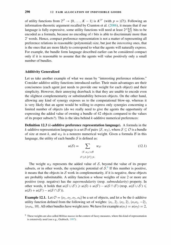
290 1 2 fair allocation of indivisible goods
of utility functions from 2O → {0, . . . , K − 1} is K2p
(with p = |O|). Following aninformation-theoretic argument recalled by Cramton et al. (2006), it means that if ourlanguage is fully expressive, some utility functions will need at least 2p ln K
ln 2 bits to beencoded as a formula, because no encoding of t bits is able to discriminate more than2t words. Hence, compact preference representation is not a matter of representing allpreference relations in reasonable (polynomial) size, but just the interesting ones, thatis the ones that are more likely to correspond to what the agents will naturally express.For example, the bundle form language described earlier can be considered compactonly if it is reasonable to assume that the agents will value positively only a smallnumber of bundles.
Additivity Generalized
Let us take another example of what we mean by “interesting preference relations.”Consider additive utility functions introduced earlier. Their main advantages are theirconciseness (each agent just needs to provide one weight for each object) and theirsimplicity. However, their annoying drawback is that they are unable to encode eventhe slightest complementarity or substitutability between objects. On the other hand,allowing any kind of synergy exposes us to the computational blow-up, whereas itis very likely that an agent would be willing to express only synergies concerning alimited number of objects (do we really need to give the agents the opportunity ofexpressing the added value of owning a bundle of 42 objects compared to the valuesof its proper subsets?). This is the idea behind k-additive numerical preferences:
Definition 12.3 (k-additive preference representation language). A formula in thek-additive representation language is a set B of pairs 〈S, wS〉, where S ⊆ O is a bundleof size at most k, and wS is a nonzero numerical weight. Given a formula B in thislanguage, the utility of each bundle S is defined as:
u(S) =∑
〈S ′,wS′ 〉∈BS ′⊆S,|S ′|≤k.
wS ′ (12.1)
The weight wS represents the added value of S , beyond the value of its propersubsets, or in other words, the synergistic potential of S .9 If this number is positive,it means that the objects in S work in complementarity, if it is negative, these objectsare probably substitutable. A utility function u whose weights of size 2 or more arepositive (resp. negative) has the supermodularity (resp. submodularity) property. Inother words, it holds that u(S ∪ S ′) � u(S) + u(S ′) − u(S ∩ S ′) (resp. u(S ∪ S ′) �u(S) + u(S ′) − u(S ∩ S ′)).
Example 12.1. Let O = {o1, o2, o3, o4} be a set of objects, and let u be the k-additiveutility function defined from the following set of weights: 〈o1, 2〉, 〈o2, 2〉, 〈o1o2,−2〉,〈o3o4, 10〉. All other bundles have weight zero. We have for example u(o1) = u(o2) = 2,
9 These weights are also called Mobius masses in the context of fuzzy measures, where this kind of representationis extensively used (see e.g., Grabisch, 1997).

1 2 .1 preferences for resource allocation problems 291
and u(o1o2) = 2 + 2 − 2, which is 2 as well. This probably means that objects o1 ando2 are substitutes (having both does not give more utility than having just one). On thecontrary, o3 and o4 alone are useless (u(o4) = u(o3) = 0), but having them together isinteresting (u(o3o4) = 10), which means that they act as complementary objects. Wecan also notice that u is neither modular, nor sub- or supermodular.
The succinctness of the language is ensured by the parameter k, that bounds the sizeof formulas representing our utility functions to
∑ki=0
(pi
) = O(pk) This parameter k
can be seen as a value that represents the trade-off between full expressivity (and for-mulas of potentially exponential size) if k = p and limited expressivity (and formulasof linear size), that is, additive functions, if k = 1.
Graphical Models
Interestingly, the k-additive preference representation coincides, for the special caseof bundle combinatorial spaces we have to deal with in resource allocation problems,with a more general preference representation language: GAI-nets (Bacchus and Grove,1995; Gonzales and Perny, 2004). The language of GAI-nets is a graphical model forpreference representation. Graphical models are a family of knowledge representationlanguages, which have been introduced decades ago in the context of uncertainty (e.g.,influence diagrams, see Howard and Matheson, 1984) probabilistic modeling (e.g.,Bayesian networks, see Pearl, 1988), constraint satisfaction (Montanari, 1974) or val-ued constraint optimization (Schiex et al., 1995). In all these contexts, graphical modelsare based upon the same components: (i) a graphical component describing directedor undirected dependencies between variables; (ii) a collection of local statements onsingle variables or small subsets of variables, compatible with the dependence struc-ture. In the particular case of GAI-nets, the preferential (in)dependence notion uponwhich this language is built is generalized additive independence (GAI), introducedby Fishburn (1970), further developed by Keeney and Raiffa (1976) in the context ofmultiattribute decision making. The k-additive representation introduced earlier can beseen as a GAI representation on a bundle space, where the size of the local relations(synergies) is explicitly bounded by k, and with no associated graphical representation.
GAI-nets are not the only graphical model for compact preference representation.Boutilier et al. (1999, 2004) have developed a very powerful and popular preferencerepresentation language: CP-nets. Unlike GAI-nets, CP-nets are dedicated to the repre-sentation of ordinal preferences. Here, the graphical structure describes the (directed)preferential dependencies between variables. The local statements, for each variable,describe the agents’ ordinal preferences on the values of the variable’s domain, givenall the possible combinations of values of its parents (hence “CP” standing for “Con-ditional Preferences”), and all other things being equal (ceteris paribus).
CP-nets have been extended to a family of preference representation languageswith different features (see e.g., Brafman et al., 2006, for TCP-nets, Boutilier et al.,2001, for UCP-nets and Wilson, 2004, for CP-theories). One of these languages,CI-nets (Bouveret et al., 2009) is especially dedicated to the representation of ordinalpreferences on sets of objects, hence well-suited to fair division problems. Formally, aCI-net N is a set of CI statements (where CI stands for Conditional Importance) of the

292 1 2 fair allocation of indivisible goods
form S+,S− : S1 ' S2 (where S+, S−, S1 and S2 are pairwise-disjoint subsets of O).The informal reading of such a statement is: “if I have all the items in S+ and noneof those in S−, I prefer obtaining all items in S1 to obtaining all those in S2, all otherthings being equal (ceteris paribus).” Formally, the interpretation of a CI-net N is thesmallest monotonic strict partial order � that satisfies each CI-statement in N , thatis, for each CI-statement S+,S− : S1 ' S2, we have S ′ ∪ S+ ∪ S1 � S ′ ∪ S+ ∪ S2 assoon as S ′ ⊆ O \ (S+ ∪ S− ∪ S1 ∪ S2).
Example 12.2. Let O = {o1, o2, o3, o4} be a set of objects, and let N be the CI-netdefined by the two following CI-statements: S1 = (o1, ∅ : o4 ' o2o3); S2 = (∅, o1, :o2o3 ' o4).
From N , we can deduce for example that o1o4 � o1o2o3 (S1) and o2o3 � o4 (S2).We can notice that obviously � is not responsive, as having o1 or not in the bundlereverses the preference between o2o3 and o4.
CI-nets are a quite natural way of expressing preferences on subsets of objects.However, as we shall see later on, computational complexity is the price to pay forthis cognitive relevance. A strict subset of this language, SCI-nets, that coincides withresponsive monotonic preferences, have been further investigated from the point ofview of fair resource allocation (Bouveret et al., 2010).
Logic-Based Languages
Another family of compact representation languages, which, unlike k-additive repre-sentation or graphical models, is not based on limited synergies, is the family logicallanguages. As we will see, propositional logic is well-suited to represent preferenceson subsets of objects, because any set of subsets of objects can be represented (oftencompactly) by a propositional formula.
In the following, given a set of objects O, we will denote by LO the propositionallanguage built upon the usual propositional operators ∧, ∨ and ¬, and one propositionalvariable for each object in O (for the sake of simplicity we use the same symbol fordenoting the object and its associated propositional variable). Each formula ϕ of LOrepresents a goal that an agent is willing to achieve. From any bundle S we can builda logical interpretation I(S) by setting all the propositional variables corresponding toan object in S to ( and the other to ⊥. A bundle S satisfies a goal ϕ (written S ϕ) ifand only if I(S) ϕ. A goal ϕ thus stands for a compact representation of the set ofall bundles that satisfy ϕ.
Example 12.3. Let O = {o1, o2, o3} be a set of objects. The goal ϕ = o1 ∨ (o2 ∧ o3)is a compact representation of the set of bundles {o1, o1o2, o1o3, o2o3, o1o2o3}.
The most obvious way of interpreting a goal as a preference relation is to considerthat the agent is only happy if the goal is satisfied, and unhappy otherwise. This leadsto a dichotomous preference relation �ϕ that is defined as follows: for each pair ofbundles 〈S,S ′〉, we have S �ϕ S ′ if and only if S ϕ or S ′ � ϕ.
This approach is not very subtle: the agent is not even able to express the tiniestpreference between two different objects she both desires. We can do better:
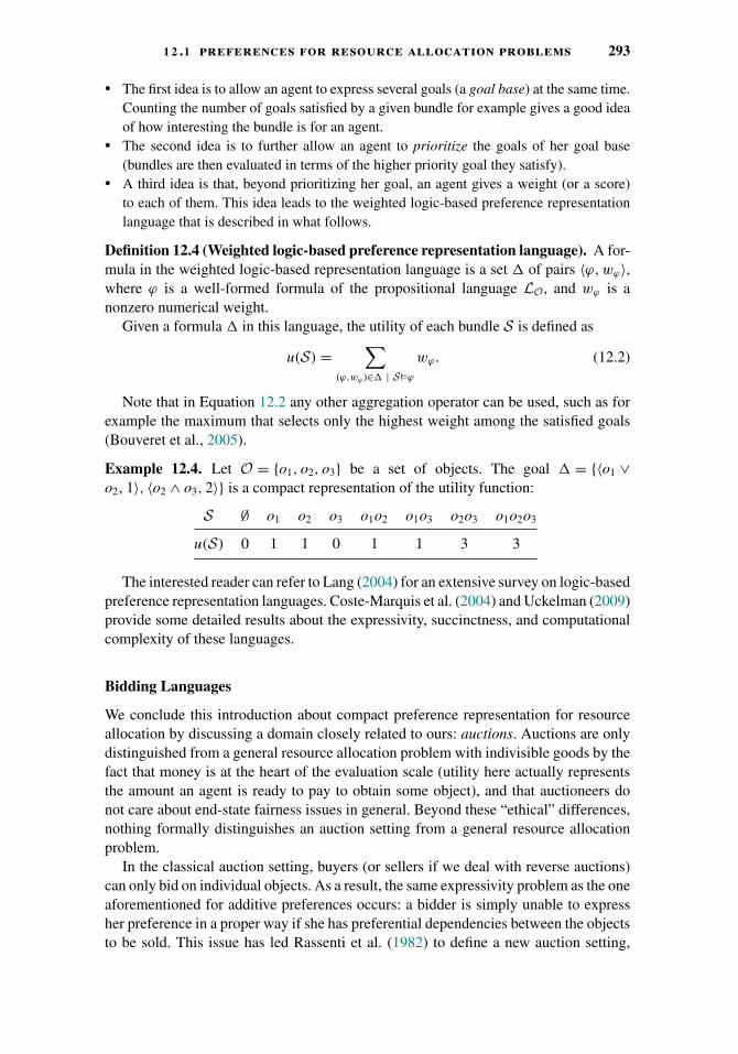
1 2 .1 preferences for resource allocation problems 293
� The first idea is to allow an agent to express several goals (a goal base) at the same time.Counting the number of goals satisfied by a given bundle for example gives a good ideaof how interesting the bundle is for an agent.
� The second idea is to further allow an agent to prioritize the goals of her goal base(bundles are then evaluated in terms of the higher priority goal they satisfy).
� A third idea is that, beyond prioritizing her goal, an agent gives a weight (or a score)to each of them. This idea leads to the weighted logic-based preference representationlanguage that is described in what follows.
Definition 12.4 (Weighted logic-based preference representation language). A for-mula in the weighted logic-based representation language is a set � of pairs 〈ϕ, wϕ〉,where ϕ is a well-formed formula of the propositional language LO, and wϕ is anonzero numerical weight.
Given a formula � in this language, the utility of each bundle S is defined as
u(S) =∑
(ϕ,wϕ )∈� | S�ϕ
wϕ. (12.2)
Note that in Equation 12.2 any other aggregation operator can be used, such as forexample the maximum that selects only the highest weight among the satisfied goals(Bouveret et al., 2005).
Example 12.4. Let O = {o1, o2, o3} be a set of objects. The goal � = {〈o1 ∨o2, 1〉, 〈o2 ∧ o3, 2〉} is a compact representation of the utility function:
S ∅ o1 o2 o3 o1o2 o1o3 o2o3 o1o2o3
u(S) 0 1 1 0 1 1 3 3
The interested reader can refer to Lang (2004) for an extensive survey on logic-basedpreference representation languages. Coste-Marquis et al. (2004) and Uckelman (2009)provide some detailed results about the expressivity, succinctness, and computationalcomplexity of these languages.
Bidding Languages
We conclude this introduction about compact preference representation for resourceallocation by discussing a domain closely related to ours: auctions. Auctions are onlydistinguished from a general resource allocation problem with indivisible goods by thefact that money is at the heart of the evaluation scale (utility here actually representsthe amount an agent is ready to pay to obtain some object), and that auctioneers donot care about end-state fairness issues in general. Beyond these “ethical” differences,nothing formally distinguishes an auction setting from a general resource allocationproblem.
In the classical auction setting, buyers (or sellers if we deal with reverse auctions)can only bid on individual objects. As a result, the same expressivity problem as the oneaforementioned for additive preferences occurs: a bidder is simply unable to expressher preference in a proper way if she has preferential dependencies between the objectsto be sold. This issue has led Rassenti et al. (1982) to define a new auction setting,
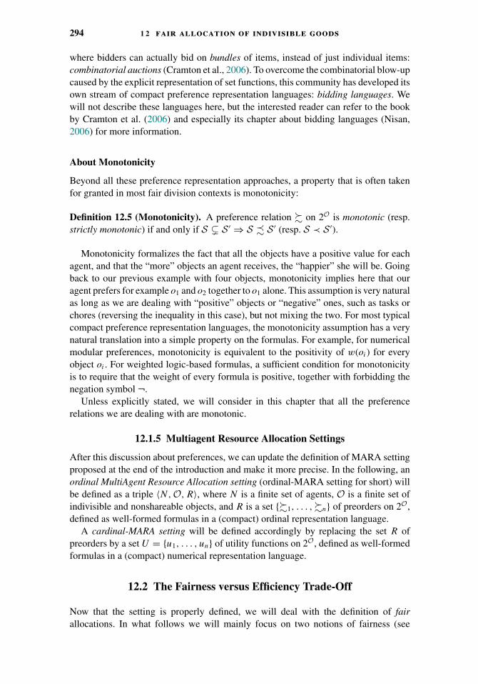
294 1 2 fair allocation of indivisible goods
where bidders can actually bid on bundles of items, instead of just individual items:combinatorial auctions (Cramton et al., 2006). To overcome the combinatorial blow-upcaused by the explicit representation of set functions, this community has developed itsown stream of compact preference representation languages: bidding languages. Wewill not describe these languages here, but the interested reader can refer to the bookby Cramton et al. (2006) and especially its chapter about bidding languages (Nisan,2006) for more information.
About Monotonicity
Beyond all these preference representation approaches, a property that is often takenfor granted in most fair division contexts is monotonicity:
Definition 12.5 (Monotonicity). A preference relation � on 2O is monotonic (resp.strictly monotonic) if and only if S � S ′ ⇒ S S ′ (resp. S ≺ S ′).
Monotonicity formalizes the fact that all the objects have a positive value for eachagent, and that the “more” objects an agent receives, the “happier” she will be. Goingback to our previous example with four objects, monotonicity implies here that ouragent prefers for example o1 and o2 together to o1 alone. This assumption is very naturalas long as we are dealing with “positive” objects or “negative” ones, such as tasks orchores (reversing the inequality in this case), but not mixing the two. For most typicalcompact preference representation languages, the monotonicity assumption has a verynatural translation into a simple property on the formulas. For example, for numericalmodular preferences, monotonicity is equivalent to the positivity of w(oi) for everyobject oi . For weighted logic-based formulas, a sufficient condition for monotonicityis to require that the weight of every formula is positive, together with forbidding thenegation symbol ¬.
Unless explicitly stated, we will consider in this chapter that all the preferencerelations we are dealing with are monotonic.
12.1.5 Multiagent Resource Allocation Settings
After this discussion about preferences, we can update the definition of MARA settingproposed at the end of the introduction and make it more precise. In the following, anordinal MultiAgent Resource Allocation setting (ordinal-MARA setting for short) willbe defined as a triple 〈N,O, R〉, where N is a finite set of agents, O is a finite set ofindivisible and nonshareable objects, and R is a set {�1, . . . ,�n} of preorders on 2O,defined as well-formed formulas in a (compact) ordinal representation language.
A cardinal-MARA setting will be defined accordingly by replacing the set R ofpreorders by a set U = {u1, . . . , un} of utility functions on 2O, defined as well-formedformulas in a (compact) numerical representation language.
12.2 The Fairness versus Efficiency Trade-Off
Now that the setting is properly defined, we will deal with the definition of fairallocations. In what follows we will mainly focus on two notions of fairness (see
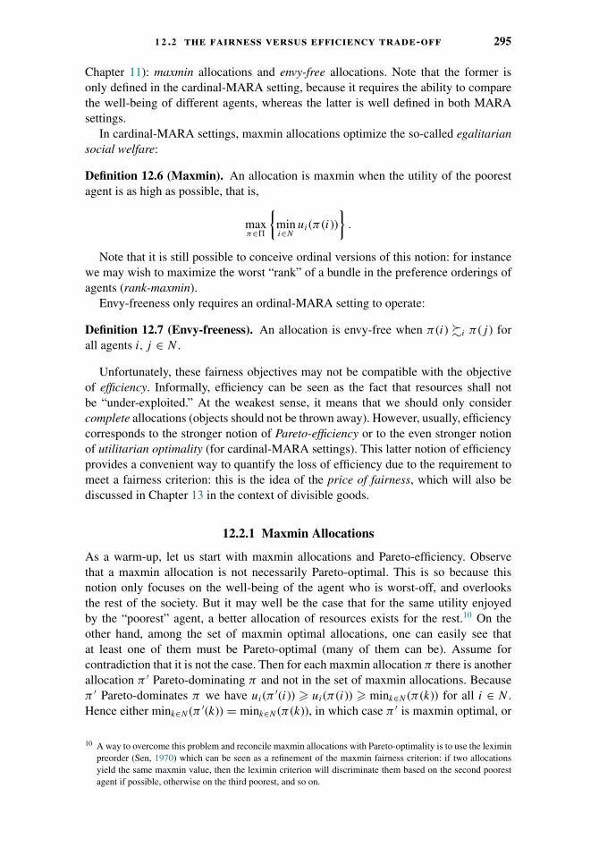
1 2 .2 the fairness versus efficiency trade-off 295
Chapter 11): maxmin allocations and envy-free allocations. Note that the former isonly defined in the cardinal-MARA setting, because it requires the ability to comparethe well-being of different agents, whereas the latter is well defined in both MARAsettings.
In cardinal-MARA settings, maxmin allocations optimize the so-called egalitariansocial welfare:
Definition 12.6 (Maxmin). An allocation is maxmin when the utility of the poorestagent is as high as possible, that is,
maxπ∈�
{mini∈N
ui(π(i))
}.
Note that it is still possible to conceive ordinal versions of this notion: for instancewe may wish to maximize the worst “rank” of a bundle in the preference orderings ofagents (rank-maxmin).
Envy-freeness only requires an ordinal-MARA setting to operate:
Definition 12.7 (Envy-freeness). An allocation is envy-free when π(i) �i π(j ) forall agents i, j ∈ N .
Unfortunately, these fairness objectives may not be compatible with the objectiveof efficiency. Informally, efficiency can be seen as the fact that resources shall notbe “under-exploited.” At the weakest sense, it means that we should only considercomplete allocations (objects should not be thrown away). However, usually, efficiencycorresponds to the stronger notion of Pareto-efficiency or to the even stronger notionof utilitarian optimality (for cardinal-MARA settings). This latter notion of efficiencyprovides a convenient way to quantify the loss of efficiency due to the requirement tomeet a fairness criterion: this is the idea of the price of fairness, which will also bediscussed in Chapter 13 in the context of divisible goods.
12.2.1 Maxmin Allocations
As a warm-up, let us start with maxmin allocations and Pareto-efficiency. Observethat a maxmin allocation is not necessarily Pareto-optimal. This is so because thisnotion only focuses on the well-being of the agent who is worst-off, and overlooksthe rest of the society. But it may well be the case that for the same utility enjoyedby the “poorest” agent, a better allocation of resources exists for the rest.10 On theother hand, among the set of maxmin optimal allocations, one can easily see thatat least one of them must be Pareto-optimal (many of them can be). Assume forcontradiction that it is not the case. Then for each maxmin allocation π there is anotherallocation π ′ Pareto-dominating π and not in the set of maxmin allocations. Becauseπ ′ Pareto-dominates π we have ui(π ′(i)) � ui(π(i)) � mink∈N (π(k)) for all i ∈ N .Hence either mink∈N (π ′(k)) = mink∈N (π(k)), in which case π ′ is maxmin optimal, or
10 A way to overcome this problem and reconcile maxmin allocations with Pareto-optimality is to use the leximinpreorder (Sen, 1970) which can be seen as a refinement of the maxmin fairness criterion: if two allocationsyield the same maxmin value, then the leximin criterion will discriminate them based on the second poorestagent if possible, otherwise on the third poorest, and so on.

296 1 2 fair allocation of indivisible goods
mink∈N (π ′(k)) > mink∈N (π(k)), in which case π is not maxmin optimal. In both case,this is a contradiction.
If we now consider the utilitarian notion of efficiency, then no guarantee can be givenon the loss of efficiency induced by the requirement to have a maxmin allocation. Letus make this statement more formal using the notion of price of fairness. The price offairness is usually defined as the ratio between the total utility of the optimal utilitarianallocation over the total utility of the best maxmin optimal allocation. The followingholds:
Theorem 12.5 (Caragiannis et al., 2012a). The price of fairness for maxmin alloca-tions is unbounded.
Proof. Suppose the preferences of n agents regarding n objects are normalized so thatthey sum up to 1, and are set as follows: each agent i (from 1 to n − 1) has utilityε for object oi , 1 − ε for object oi+1, and 0 for the other objects, while agent n hasonly utility 1 for object on. The maxmin allocation assigns object oi to each agent i,and thus yields 1 + (n − 1) · ε overall when we sum utilities. But giving to each agenti ∈ 1, . . . , n − 1 object oi+1 (and object 1 to anyone) yields an overall (n − 1) · (1 − ε).Hence, the ratio is unbounded as n grows.
12.2.2 Envy-Freeness
As an obvious first remark, note that a partial allocation where each good is thrownaway is obviously envy-free: all agents own the same empty bundle, so they cannotenvy each other. Thus, in this section we will focus on the nontrivial case of completeallocations.
First, as with the maxmin criterion, an envy-free allocation is not necessarily Pareto-efficient, as shown in the following example:
Example 12.6. Let O = {o1, o2, o3, o4} be a set of objects shared by two agents.Assume u1 (S) = 1{{o1,o2}}(S) and u2 (S) = 1{{o3,o4}}(S), where 1. is the indicator func-tion. Then, the allocation where agent 1 owns {o1, o3} and agent 2 owns {o2, o4} iscomplete and envy-free, but not Pareto efficient: giving {o1, o2} and {o3, o4} respec-tively to agents 1 and 2 will strictly increase their utility function.
Next, it is easy to show that there does not always exist an envy-free completeallocation. Consider the case where two agents share a single good, and suppose thisgood is preferred by both agents to the empty bundle. Then, the agent owning thegood will be envied by the other agent. More generally, the probability of existenceof complete and envy-free allocation has actually been further investigated in a recentwork by Dickerson et al. (2014). In particular, this work shows analytically that underseveral assumptions on the probability distribution of the agents’ (additive) preferences,an envy-free allocation is unlikely to exist up to a given threshold on the ratio betweenthe number of goods and the number of agents, and very likely to exist beyond.Experimental results show an interesting phenomenon of phase-transition.
Finally, consider the utilitarian notion of efficiency. Similarly to the price of fair-ness, the price of envy-freeness has been defined by Caragiannis et al. (2012a) as
1 2 .2 the fairness versus efficiency trade-off 297
the ratio between the total utility of the optimal utilitarian allocation over the totalutility of the best envy-free allocation. Caragiannis et al. (2012a) show that theprice of envy-freeness is � (n). So as more and more agents appear in the system,the gap between envy-free allocations and optimal allocations will grow at a linearrate.
12.2.3 Other Fairness Criteria
Beyond maxmin fairness and envy-freeness, proportionality is another prominent fair-ness criterion. This property, coined by Steinhaus (1948) in the context of continuousfair division (cake-cutting) problems, states that each agent should get from the allo-cation at least one nth of the total utility she would have received if she were alone.Obviously, this criterion is related to maxmin fairness when utility are normalized (eachagent gives the same value to the entire set of objects): if there exists an allocationthat satisfies proportionality, then any maxmin-optimal allocation satisfies it. As wewill see in Chapter 13, it is always possible to find an allocation that satisfies propor-tionality. In the case of two agents, the example procedure given in the introductionof the chapter (Alice cuts, Bob chooses) obviously guarantees a proportional share toboth agents. Once again, things turn bad when we switch to indivisible objects (justconsider again one object and two agents, no allocation can give her fair share to eachagent).
Even if it is not possible to guarantee one nth of the resource to each agent, Demkoand Hill (1988) have shown that under additive numerical preferences it is alwayspossible to find an allocation guaranteeing a given amount of utility (only depend-ing on the maximum weight α given by the agents to the objects) to each agent.Markakis and Psomas (2011) have significantly extended this result, first by showingthat it is actually possible to guarantee that the minimal amount of utility received byeach agent i depends on the maximum weight αi given by this agent to the objects,and secondly by exhibiting a deterministic polynomial-time algorithm to computeit. The same idea has been used by Gourves et al. (2013), who further refine theseresults by constructively exhibiting a stronger lower bound, that also works for fairdivision problems with a particular kind of admissibility constraints represented as amatroid.
Another approach has been proposed by Budish (2011). Instead on focusing on themaximal fraction of absolute utility it is possible to guarantee to each agent, Budish(2011) proposes to start from the “I cut you choose” protocol described earlier inthe divisible case, and to adapt it to the indivisible case. According to this definitionof fairness, every agent i should receive from the allocation at least what she wouldreceive in the worst case if she had to partition the objects into n bundles and letthe other n − 1 agents choose first. In other words, each agent should receive at leastthe best (max), among all possible allocations (cuts), of the worst (min) share of thisallocation: Budish (2011) calls it the maximin share. Obviously, in the cake-cuttingcase, this notion coincides with proportionality.
Example 12.7. Consider a MARA setting involving two agents with additive prefer-ences, and four objects {o1, o2, o3, o4}. Let agent 1’s preferences be defined as follows:

298 1 2 fair allocation of indivisible goods
u1(o1) = 7, u1(o2) = 2, u1(o3) = 6 and u1(o4) = 10. Then agent 1’s maximin share is12, associated to partition {o1o3, o2o4}.
Contrary to proportionality, in the case of additive preferences, maximin share guar-antee is almost always possible to satisfy (Bouveret and Lemaıtre, 2014). Actually,Procaccia and Wang (2014) have exhibited some MARA-settings where no alloca-tion guaranteeing maximin shares to everyone can be found, but these instances arerather rare.11 Moreover, Bouveret and Lemaıtre (2014) notice that in the special case ofadditive preferences, not only envy-freeness implies proportionality, but also propor-tionality implies maximin share guarantee. It means that these properties form a scaleof fairness criteria, from the strongest to the weakest.12 This suggests another solutionto the fairness versus efficiency trade-off: try to satisfy envy-freeness if possible; ifnot, try to satisfy proportionality if you can; and finally, as a fallback fairness criterion,maximin share guarantee is almost always possible to satisfy.
12.3 Computing Fair Allocations
We will now see how challenging computing optimal fair allocations is. To achieve this,we will among other things study the computational complexity of decision problemsassociated with the computation of fair allocations. The input of these decision problemswill include the preference profiles encoded in a given representation language. Notethat if a preference profile is represented with a formula whose size is superpolynomialin p and n, then even if the decision problem is computationally easy, finding afair allocation may remain prohibitive in practice—hence the relevance of compactrepresentation languages discussed in the previous section.
12.3.1 Maxmin Allocations
We start with a bad news: if we make no assumption on the preferences of agents(beyond monotonicity), then not only is computing an optimal maxmin allocationcomputationally hard, but even computing an approximation is (Golovin, 2005). Theargument is simple, and based as usual on a problem known to be hard. In the partitionproblem, we are given a collection of (positive) integers C = 〈c1, . . . , cq〉 such that∑q
i=1 ci = 2k, and we are asked whether there exists I ⊆ {1, . . . , n} with∑
i∈I ci = k.But now take O = C and set the utility functions of two agents as follows:
u(S) ={
1 if∑
x∈S x � k
0 otherwise .
The only situation where an allocation with social welfare 1 can be obtained is whenagents receive a bundle such that
∑x∈S x = k, otherwise any allocation yields utility
0 (because at least one agent enjoys utility 0). But then any approximation would haveto distinguish between these cases, which requires to solve partition. The careful
11 They also show that it is always possible to guarantee at least 2/3 of the maximin share to everyone.12 Actually there are two additional criteria in the scale, which we do not discuss here for the sake of clarity and
conciseness.
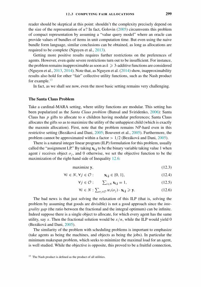
1 2 .3 computing fair allocations 299
reader should be skeptical at this point: shouldn’t the complexity precisely depend onthe size of the representation of u? In fact, Golovin (2005) circumvents this problemof compact representation by assuming a “value query model” where an oracle canprovide values of bundles of items in unit computation time. But even using the naivebundle form language, similar conclusions can be obtained, as long as allocations arerequired to be complete (Nguyen et al., 2013).
Getting more positive results requires further restrictions on the preferences ofagents. However, even quite severe restrictions turn out to be insufficient. For instance,the problem remains inapproximable as soon as k � 3-additive functions are considered(Nguyen et al., 2013, 2014). Note that, as Nguyen et al. (2014) show, inapproximabilityresults also hold for other “fair” collective utility functions, such as the Nash productfor example.13
In fact, as we shall see now, even the most basic setting remains very challenging.
The Santa Claus Problem
Take a cardinal-MARA setting, where utility functions are modular. This setting hasbeen popularized as the Santa Claus problem (Bansal and Sviridenko, 2006): SantaClaus has p gifts to allocate to n children having modular preferences; Santa Clausallocates the gifts so as to maximize the utility of the unhappiest child (which is exactlythe maxmin allocation). First, note that the problem remains NP-hard even in thisrestrictive setting (Bezakova and Dani, 2005; Bouveret et al., 2005). Furthermore, theproblem cannot be approximated within a factor > 1/2 (Bezakova and Dani, 2005).
There is a natural integer linear program (ILP) formulation for this problem, usuallycalled the “assignment LP.” By taking xi,j to be the binary variable taking value 1 whenagent i receives object oj , and 0 otherwise, we set the objective function to be themaximization of the right-hand side of Inequality 12.6:
maximize y, (12.3)
∀i ∈ N, ∀j ∈ O : xi,j ∈ {0, 1}, (12.4)
∀j ∈ O :∑
i∈N xi,j = 1, (12.5)
∀i ∈ N :∑
oj∈O wi(oj ) · xi,j � y. (12.6)
The bad news is that just solving the relaxation of this ILP (that is, solving theproblem by assuming that goods are divisible) is not a good approach since the inte-grality gap (the ratio between the fractional and the integral optimum) can be infinite.Indeed suppose there is a single object to allocate, for which every agent has the sameutility, say x. Then the fractional solution would be x/n, while the ILP would yield 0(Bezakova and Dani, 2005).
The similarity of the problem with scheduling problems is important to emphasize(take agents as being the machines, and objects as being the jobs). In particular theminimum makespan problem, which seeks to minimize the maximal load for an agent,is well studied. While the objective is opposite, this proved to be a fruitful connection,
13 The Nash product is defined as the product of all utilities.

300 1 2 fair allocation of indivisible goods
and motivated the use of (adapted) sophisticated rounding techniques (Lenstra et al.,1990). Bezakova and Dani (2005) were among the first to exploit this connection. Theyused job truncations techniques to propose an O(n) approximation, later improved toO( 1√
n log3 n) by Asadpour and Saberi (2010).
Linear programming is not the only possible approach to this problem: branch andbound techniques have also been investigated (Dall’Aglio and Mosca, 2007). For thistype of algorithms, the quality of the bound is a crucial component. Dall’Aglio andMosca (2007) use the “adjusted winner” procedure (that we discuss later on in thischapter) to compute this bound.
12.3.2 Computing Envy-Free or Low-Envy Allocations
There is a simple algorithm which always returns an envy-free allocation: throw allthe objects away! However, as discussed already, as soon as a very minimal efficiencyrequirement of completeness is introduced, an envy-free allocation may not exist. Infact, it is computationally hard to decide whether such an allocation exists (Liptonet al., 2004). If we now ask for an allocation which meets both envy-freeness andPareto-optimality, then for most compact representation languages the problem liesabove NP (Bouveret and Lang, 2008). More precisely, this problem is �P
2-completefor most logic-based languages introduced in Section 12.1, including the very simplelanguage leading to dichotomous preferences. It also turns out that the combinatorialnature of the domain plays little role here: even in additive domains, deciding whetherthere exists an efficient and envy-free allocation is �P
2-complete (de Keijzer et al.,2009).
Given this, a perhaps more realistic objective is to seek to minimize the “degreeof envy” of the society. There are several ways to define such a metric. For example,Cavallo (2012) defines the rate of envy as the average envy of all agents. Here wefollow Lipton et al. (2004) in their definitions:
eij (π) = max{0, ui(π(j )) − ui(π(i))}.
Now the envy of the allocation is taken to be the maximal envy among any pair ofagents, that is,
e(π) = max{eij (π) | i, j ∈ N}. (12.7)
Allocations with Bounded Maximal Envy
One may ask whether allocations with bounded maximal envy can be found. Thequestion is raised by Dall’Aglio and Hill (2003) and later addressed by Lipton et al.(2004). We will see that such bounds can be obtained, by taking as a parameter themaximal marginal utility of a problem, noted α. The marginal utility of a good oj , givenan agent i and a bundle S , is the amount of additional utility that this object yieldswhen taken together with the bundle. Then the maximal marginal utility is simply themaximal value among all agents, bundles, and objects. In an additive setting, this isthus simply the highest utility that an agent assigns to a good.

1 2 .3 computing fair allocations 301
The result by Lipton et al. (2004)—which improves upon a first bound of O(αn3/2)given by Dall’Aglio and Hill (2003)—is then simply stated:
Theorem 12.8 (Lipton et al., 2004). It is always possible to find an allocation whoseenvy is bounded by α, the maximal marginal utility of the problem.
Proof sketch. First, we introduce the notion of the envy graph associated with anallocation π , where nodes are agents and there is an edge from i to j when i envies j .Now take a cycle in this envy graph: a key observation is that by rotating the bundlesheld by agents in the direction opposite to that of the cycle (so that each agent gets thebundle of the agent he envies), we necessarily “break the envy cycle” at some point.This is so because the utility of each agent in this cycle is increased at each step ofthis rotation. Furthermore, agents outside the cycle are unaffected by this reallocation.Now consider the following procedure. Goods are allocated one by one. First allocateone good arbitrarily. Now consider the end of round k, and suppose {o1, . . . , ok} havebeen allocated, and that envy is bounded by α. At round k + 1 we build the envy graph.Next we rotate the bundles as previously described. As already observed, at some pointthere must be an agent i that no one envies. We then allocate object ok+1 to this agenti. Envy is thus at most α.
Example 12.9. Let O = {o1, o2, o3, o4, o5} be a set of objects, and let {1, 2, 3} be threeagents whose additive preferences are defined as follows:
S o1 o2 o3 o4 o5
u1(S) 1 2 5 3 7u2(S) 2 6 8 1 5u3(S) 5 4 4 3 1
The maximal marginal utility is 8. We know that by applying the procedure we areguaranteed to obtain an allocation with a degree of envy at most 8. Suppose we allocatethe first three items oi to agent i, we thus get π(1) = {o1}, π(2) = {o2}, and π(3) = {o3}.At this step of the procedure, the envy graph is depicted in (i). For convenience weindicate the degree of envy on each arrow. There are two cycles. Let us consider forinstance the cycle (1,3), and rotate (this corresponds to simply swapping the resourcesof agents 1 and 3 here). It happens to be sufficient to remove the cycle: we obtain thenew envy graph (ii). Now we wish to allocate o4. No one envies 2 nor 3, so we can forinstance allocate o4 to 2, resulting in (iii). The graph is without cycle. We can now giveo5 to agent 3, thus obtaining (iv), with a degree of envy of 3.
302 1 2 fair allocation of indivisible goods
Note that in that case, by performing a final rotation, we could obtain en envy-freeallocation.
Observe that the procedure makes no assumption on the preferences of agents.The result thus shows that it is always possible to have an allocation bounded by thehighest marginal value. Of course, such a bound is tight, as is easily observed by ascenario involving a single good and two agents with the same utility for it. In general,however, for a given instance, allocations with a much lower envy than this bound willexist.
Low-Envy Allocations
Is it possible to design algorithms returning an allocation with minimal envy, or at leastan approximation of it? A critical problem is that in the case of general preferences, theamount of information that needs to be transmitted to the algorithm is prohibitive (seeSection 12.4). It is thus natural to consider the same question in restricting the domainconsidered.
Another technical issue occurs: the minimum degree of envy as defined byEquation (12.7) is 0 when the allocation is envy-free. While this an intuitive require-ment, it has an undesirable consequence: any finite approximation would have to beable to distinguish an envy-free allocation. Unfortunately, as we have seen, this prob-lem is hard, even in the case of modular preferences. Thus, unless P = NP, there is nohope for approximation here (remember the same line of argumentation was used toshow inapproximability for maxmin allocations).
To circumvent this, a different measure of envy is considered. The minimum envy-ratio is defined as
max
{1,
ui(πj )
ui(πi)
}.
When the objective function is to minimize this measure, positive results can beobtained. Lipton et al. (2004) were the first to address this version of the problem. Theymade the additional assumption that agents have the same preferences. In this context,the greedy procedure proposed by Graham (1969) in the context of scheduling yields a1.4-approximation. The procedure is fairly simple: rank the goods in decreasing order,then allocate them one by one, to the agent whose current bundle has least value.But Lipton et al. (2004) went further: they showed that it is possible to achieve anapproximation arbitrarily close to 1 with an algorithm running in polynomial time inthe input size (in other words, a Polynomial-Time Approximation Scheme). When thenumber of agents is bounded, it is even possible to get an FPTAS for this minimizationproblem. Recently, Nguyen and Rothe (2015) took up this research agenda. When thenumber of agents is bounded, they obtain an FPTAS for this minimization problem(and other degree measures), even when agents have different preferences. On the otherhand, they showed that when the number of agents is part of the input, it will not bepossible to obtain (in polynomial time) an approximation factor better than 3/2, underthe usual P �= NP assumption.

1 2 .3 computing fair allocations 303
Envy-Freeness and Ordinal Preferences
Let us conclude this overview of computational aspects of envy-freeness with a quicklook at ordinal preferences. An interesting feature of envy-freeness is that this notiondoes not require any interpersonal comparison of preferences. As a result, envy-freenessis a purely ordinal notion: this fairness criterion is properly defined as soon as theagents are able to compare pairs of bundles (which is not the case for maxmin fairness,requiring cardinal preferences). The ordinal analogous of the problem studied by Liptonet al. (2004) for numerical preferences, namely, the problem of finding an efficient andenvy-free allocation with ordinal preferences (using pairwise dominance for liftingpreferences from objects to bundles) has been studied by Brams et al. (2004) andBrams and King (2005) and later by Bouveret et al. (2010) and Aziz et al. (2014d).
The main difficulty here is that, unlike additivity for numerical preferences, onlyrequiring responsiveness (and monotonicity, for the two latter references) leaves manypairs of bundles incomparable. For example, if we have o1 ' o2 ' o3 ' o4, responsive-ness implies that o1o2 � o3o4, but leaves o1o4 and o2o3 incomparable. This calls foran extended version of envy-freeness that takes into account incomparabilities. Bramset al. (2004); Bouveret et al. (2010) propose the two notions of possible and necessaryenvy:14 basically, agent i possibly (resp. necessarily) envies agent j if π(i) ��i π(j )(resp. π(j ) �i π(i)). The recent work of Aziz et al. (2014d) further extends and refinesthese notions by introducing a new definition of ordinal dominance based on stochasticdominance.
On the positive side, it turns out that the problem of determining whether a pos-sible envy-free efficient allocation exists is in P (Bouveret et al., 2010) for strictpreferences, for different notions of efficiency (completeness, possible and necessaryPareto-efficiency). On the negative side, things seem to be harder (NP-complete) fornecessary envy-freeness, and as soon as ties are allowed (Aziz et al., 2014d). Note alsothat in the case of ordinal preferences, defining measures of envy makes less sense thanfor numerical preferences. That means that it seems difficult to use approximation tocircumvent the computational complexity of the problem.
12.3.3 Other Fairness Measures
In this section we have looked in details at the computation of maxmin or low-envyallocations. Of course, there are many other criteria of fairness of interest. In particular,it is natural to not only focus on the worst-off agent, but to define a more generalmeasure of the inequality of the society and to rely on a generalized Gini social-evaluation function. This class of functions is also known as ordered weighted averages(Yager, 1988). The computation of these functions has been studied by Lesca and Perny(2010). They investigate in particular how techniques of linear programming (such asthe one mentioned in Section 12.3.1) can be adapted so to handle these problems.Recently, the problem of computing inequality indices in combinatorial domains hasbeen considered by Endriss (2013). Also, Vetschera (2010) came up with an approach
14 Actually Brams et al. (2004) use a different terminology, but the idea is the same.
304 1 2 fair allocation of indivisible goods
generalizing the branch and bound approach of Dall’Aglio and Mosca (2007) to a widerclass of objective functions: more precisely, for any setting involving the division ofindivisible goods between two agents, and for which the objective function is maximumwhen the utilities of both players are equal (in the hypothetical continuous case). Inthat case, the bound based on the “adjusted winner” split, which will be presented inSection 12.4.1, is not valid any longer.
12.4 Protocols for Fair Allocation
The centralized “one-shot” approaches to fair resource allocation we have consideredso far work in two steps: first the agents fully reveal their preferences (may thembe ordinal or numerical) to the benevolent arbitrator, then this arbitrator computes asatisfactory allocation (thanks to an algorithm) and gives the objects to the agents. Thisapproach has two main drawbacks: (i) the elicitation process can be very expensiveor agents may not be willing to fully reveal their preferences; and (ii) agents may bereluctant to accept a solution computed as a black-box.
Regarding (i), there is not much we can do in the worst case : when preferences arenot modular, the communication load that is required to compute optimal (or indeedapproximated) fair solutions becomes a fundamental barrier. This can be stated moreformally:
Theorem 12.10 (Lipton et al., 2004; Golovin, 2005). Any deterministic algorithmwould require an exponential number of queries to compute any finite approximationfor the minimal envy allocation (Lipton et al., 2004) or the maxmin allocation (Golovin,2005).
Such lower bounds can be obtained by borrowing techniques from the communica-tion complexity literature (see also Chapter 10).
The incremental protocols we discuss in this section take a different approach: theyprescribe “simple” actions to be taken by the agents at different stages of the process(comparing two bundles, choosing an item, etc.), and they (typically) do not requireheavy computation from the central authority. They sometimes do not involve anycentral computation at all (beyond verification of the legality of agents’ actions) norpreference elicitation, and may even work in the absence of a central authority in somecases, as we shall see.
Before we go on and present original protocols, note that some of the algorithmspresented earlier in this chapter can be readily interpreted as protocols. This is true inparticular of the procedure of Lipton et al. (2004): allocate items sequentially, and eachtime a new item is assigned, ask agents to point to agents they envy (note that this doesnot require to elicit preferences). When a cycle occurs, rotate the bundles as indicatedin the procedure, and ask again agents who they envy, and so on. Of course, as we havealready seen, the guarantees of such a protocol are not so good. We will see that betterguarantees can be given, at the price of restrictions on the number of agents, or on thetype of preferences.

1 2 .4 protocols for fair allocation 305
12.4.1 Protocols for Two Agents
The Adjusted Winner Procedure
This procedure has been used in various contexts (Brams and Taylor, 2000). It worksfor two agents, with additive utility functions. At the end of the procedure, one itemmay need to get split, but as we do not know beforehand which one, it has to assumethat all items are divisible. The technique is nevertheless inspiring, and can be usedto compute a bound in the indivisible case (Dall’Aglio and Mosca, 2007), as alreadymentioned.
In the first phase of the algorithm (the “winning phase”), goods are allocated effi-ciently, that is, each good is assigned to the agent who values it the most. At the endof this stage, either u1 = u2 and we are done, or some agent (say r , the richest) has ahigher utility than the other (say p, the poorest) and the “adjusting phase” can begin.During this phase, goods are transferred from the richest to the poorest, in increasingorder of the ratio ur (o)
up(o) (note that the ratio is necessarily � 1). The algorithm stops wheneither both agents enjoy the same utility, or the richest becomes the poorest. Supposethis happens under the transfer of good g: then g is split so as to attain equitability, thatis, the utility of both agents is equal. To get this equitable outcome, the richest gets afraction of g computed as follows:
up(g) + up(π(p) \ {g}) − ur (π(r) \ {g})ur (g) + up(g)
The allocation is thus also a maxmin allocation. In fact, it has several desirableproperties:
Theorem 12.11 (Brams and Taylor, 2000). The adjusted winner procedure returnsan equitable, envy-free, and Pareto-optimal allocation.
Recall that here “equitable” means that the two agents enjoy the same utility at theend of the protocol.
Example 12.12. Let O = {o1, o2, o3, o4, o5} be a set of objects.
S o1 o2 o3 o4 o5
u1(S) 1 2 5 3 7u2(S) 2 6 8 1 5
After the winning phase, agent 2 gets {o1, o2, o3} and agent 1 gets {o4, o5}. The utilityof agent 2 is 2 + 6 + 8 = 16 while the utility of agent 1 is 10. Agent 2 will transfergoods to agent 1, starting with o3 (with ratio 8
5 , while o1 has 21 , and o2 has 6
2 ). Butonce we do that agent 1 becomes the richest: the good o3 has to be split, with agent2 obtaining (5 + 10 − 8)/13 = 7/13 of the good g (and the rest for agent 1). Thisprovides each agent a utility * 12.3.
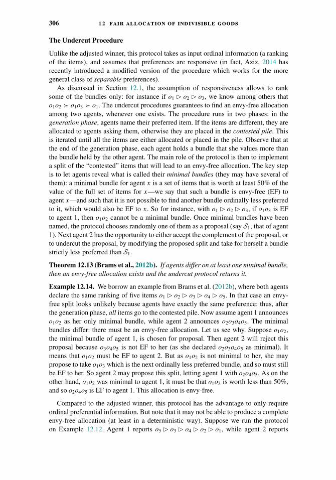
306 1 2 fair allocation of indivisible goods
The Undercut Procedure
Unlike the adjusted winner, this protocol takes as input ordinal information (a rankingof the items), and assumes that preferences are responsive (in fact, Aziz, 2014 hasrecently introduced a modified version of the procedure which works for the moregeneral class of separable preferences).
As discussed in Section 12.1, the assumption of responsiveness allows to ranksome of the bundles only: for instance if o1 � o2 � o3, we know among others thato1o2 � o1o3 � o1. The undercut procedures guarantees to find an envy-free allocationamong two agents, whenever one exists. The procedure runs in two phases: in thegeneration phase, agents name their preferred item. If the items are different, they areallocated to agents asking them, otherwise they are placed in the contested pile. Thisis iterated until all the items are either allocated or placed in the pile. Observe that atthe end of the generation phase, each agent holds a bundle that she values more thanthe bundle held by the other agent. The main role of the protocol is then to implementa split of the “contested” items that will lead to an envy-free allocation. The key stepis to let agents reveal what is called their minimal bundles (they may have several ofthem): a minimal bundle for agent x is a set of items that is worth at least 50% of thevalue of the full set of items for x—we say that such a bundle is envy-free (EF) toagent x—and such that it is not possible to find another bundle ordinally less preferredto it, which would also be EF to x. So for instance, with o1 � o2 � o3, if o1o3 is EFto agent 1, then o1o2 cannot be a minimal bundle. Once minimal bundles have beennamed, the protocol chooses randomly one of them as a proposal (say S1, that of agent1). Next agent 2 has the opportunity to either accept the complement of the proposal, orto undercut the proposal, by modifying the proposed split and take for herself a bundlestrictly less preferred than S1.
Theorem 12.13 (Brams et al., 2012b). If agents differ on at least one minimal bundle,then an envy-free allocation exists and the undercut protocol returns it.
Example 12.14. We borrow an example from Brams et al. (2012b), where both agentsdeclare the same ranking of five items o1 � o2 � o3 � o4 � o5. In that case an envy-free split looks unlikely because agents have exactly the same preference: thus, afterthe generation phase, all items go to the contested pile. Now assume agent 1 announceso1o2 as her only minimal bundle, while agent 2 announces o2o3o4o5. The minimalbundles differ: there must be an envy-free allocation. Let us see why. Suppose o1o2,the minimal bundle of agent 1, is chosen for proposal. Then agent 2 will reject thisproposal because o3o4o5 is not EF to her (as she declared o2o3o4o5 as minimal). Itmeans that o1o2 must be EF to agent 2. But as o1o2 is not minimal to her, she maypropose to take o1o3 which is the next ordinally less preferred bundle, and so must stillbe EF to her. So agent 2 may propose this split, letting agent 1 with o2o4o5. As on theother hand, o1o2 was minimal to agent 1, it must be that o1o3 is worth less than 50%,and so o2o4o5 is EF to agent 1. This allocation is envy-free.
Compared to the adjusted winner, this protocol has the advantage to only requireordinal preferential information. But note that it may not be able to produce a completeenvy-free allocation (at least in a deterministic way). Suppose we run the protocolon Example 12.12. Agent 1 reports o5 � o3 � o4 � o2 � o1, while agent 2 reports
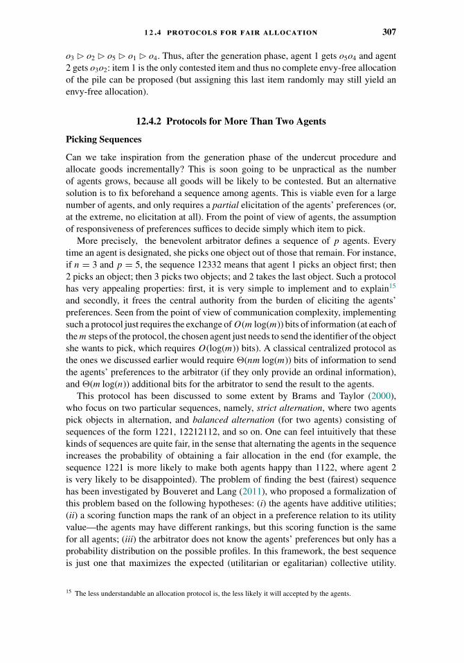
1 2 .4 protocols for fair allocation 307
o3 � o2 � o5 � o1 � o4. Thus, after the generation phase, agent 1 gets o5o4 and agent2 gets o3o2: item 1 is the only contested item and thus no complete envy-free allocationof the pile can be proposed (but assigning this last item randomly may still yield anenvy-free allocation).
12.4.2 Protocols for More Than Two Agents
Picking Sequences
Can we take inspiration from the generation phase of the undercut procedure andallocate goods incrementally? This is soon going to be unpractical as the numberof agents grows, because all goods will be likely to be contested. But an alternativesolution is to fix beforehand a sequence among agents. This is viable even for a largenumber of agents, and only requires a partial elicitation of the agents’ preferences (or,at the extreme, no elicitation at all). From the point of view of agents, the assumptionof responsiveness of preferences suffices to decide simply which item to pick.
More precisely, the benevolent arbitrator defines a sequence of p agents. Everytime an agent is designated, she picks one object out of those that remain. For instance,if n = 3 and p = 5, the sequence 12332 means that agent 1 picks an object first; then2 picks an object; then 3 picks two objects; and 2 takes the last object. Such a protocolhas very appealing properties: first, it is very simple to implement and to explain15
and secondly, it frees the central authority from the burden of eliciting the agents’preferences. Seen from the point of view of communication complexity, implementingsuch a protocol just requires the exchange of O(m log(m)) bits of information (at each ofthe m steps of the protocol, the chosen agent just needs to send the identifier of the objectshe wants to pick, which requires O(log(m)) bits). A classical centralized protocol asthe ones we discussed earlier would require �(nm log(m)) bits of information to sendthe agents’ preferences to the arbitrator (if they only provide an ordinal information),and �(m log(n)) additional bits for the arbitrator to send the result to the agents.
This protocol has been discussed to some extent by Brams and Taylor (2000),who focus on two particular sequences, namely, strict alternation, where two agentspick objects in alternation, and balanced alternation (for two agents) consisting ofsequences of the form 1221, 12212112, and so on. One can feel intuitively that thesekinds of sequences are quite fair, in the sense that alternating the agents in the sequenceincreases the probability of obtaining a fair allocation in the end (for example, thesequence 1221 is more likely to make both agents happy than 1122, where agent 2is very likely to be disappointed). The problem of finding the best (fairest) sequencehas been investigated by Bouveret and Lang (2011), who proposed a formalization ofthis problem based on the following hypotheses: (i) the agents have additive utilities;(ii) a scoring function maps the rank of an object in a preference relation to its utilityvalue—the agents may have different rankings, but this scoring function is the samefor all agents; (iii) the arbitrator does not know the agents’ preferences but only has aprobability distribution on the possible profiles. In this framework, the best sequenceis just one that maximizes the expected (utilitarian or egalitarian) collective utility.
15 The less understandable an allocation protocol is, the less likely it will accepted by the agents.
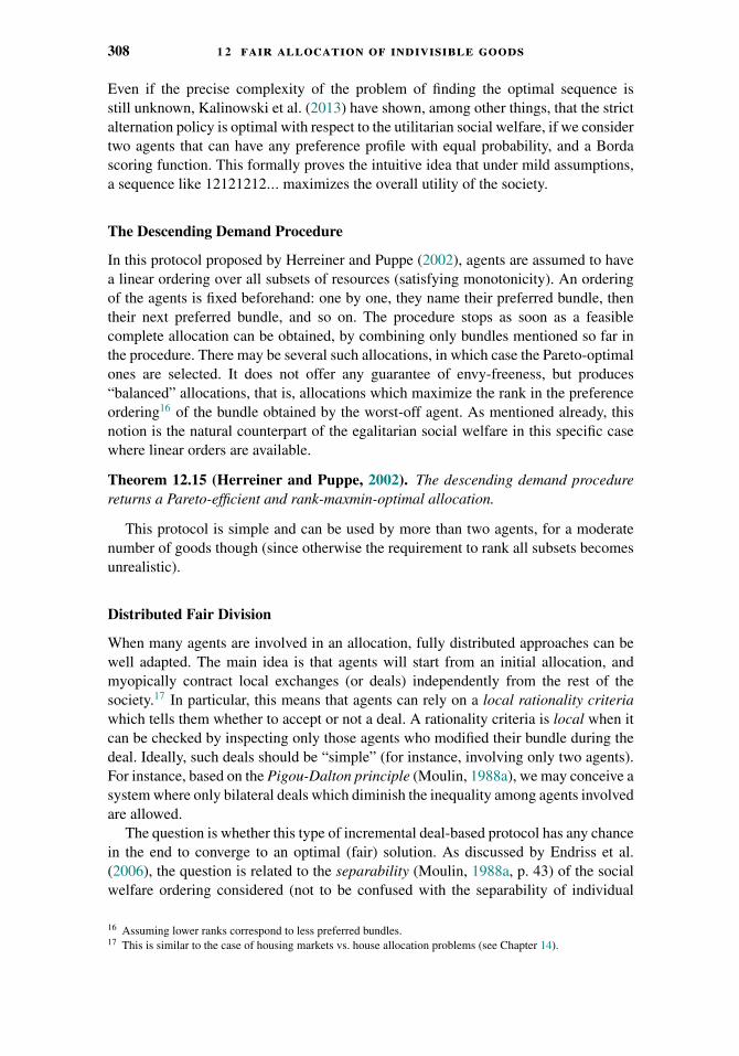
308 1 2 fair allocation of indivisible goods
Even if the precise complexity of the problem of finding the optimal sequence isstill unknown, Kalinowski et al. (2013) have shown, among other things, that the strictalternation policy is optimal with respect to the utilitarian social welfare, if we considertwo agents that can have any preference profile with equal probability, and a Bordascoring function. This formally proves the intuitive idea that under mild assumptions,a sequence like 12121212... maximizes the overall utility of the society.
The Descending Demand Procedure
In this protocol proposed by Herreiner and Puppe (2002), agents are assumed to havea linear ordering over all subsets of resources (satisfying monotonicity). An orderingof the agents is fixed beforehand: one by one, they name their preferred bundle, thentheir next preferred bundle, and so on. The procedure stops as soon as a feasiblecomplete allocation can be obtained, by combining only bundles mentioned so far inthe procedure. There may be several such allocations, in which case the Pareto-optimalones are selected. It does not offer any guarantee of envy-freeness, but produces“balanced” allocations, that is, allocations which maximize the rank in the preferenceordering16 of the bundle obtained by the worst-off agent. As mentioned already, thisnotion is the natural counterpart of the egalitarian social welfare in this specific casewhere linear orders are available.
Theorem 12.15 (Herreiner and Puppe, 2002). The descending demand procedurereturns a Pareto-efficient and rank-maxmin-optimal allocation.
This protocol is simple and can be used by more than two agents, for a moderatenumber of goods though (since otherwise the requirement to rank all subsets becomesunrealistic).
Distributed Fair Division
When many agents are involved in an allocation, fully distributed approaches can bewell adapted. The main idea is that agents will start from an initial allocation, andmyopically contract local exchanges (or deals) independently from the rest of thesociety.17 In particular, this means that agents can rely on a local rationality criteriawhich tells them whether to accept or not a deal. A rationality criteria is local when itcan be checked by inspecting only those agents who modified their bundle during thedeal. Ideally, such deals should be “simple” (for instance, involving only two agents).For instance, based on the Pigou-Dalton principle (Moulin, 1988a), we may conceive asystem where only bilateral deals which diminish the inequality among agents involvedare allowed.
The question is whether this type of incremental deal-based protocol has any chancein the end to converge to an optimal (fair) solution. As discussed by Endriss et al.(2006), the question is related to the separability (Moulin, 1988a, p. 43) of the socialwelfare ordering considered (not to be confused with the separability of individual
16 Assuming lower ranks correspond to less preferred bundles.17 This is similar to the case of housing markets vs. house allocation problems (see Chapter 14).
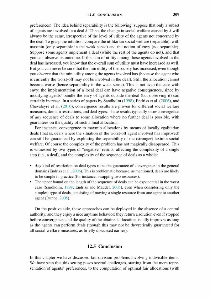
1 2 .5 conclusion 309
preferences). The idea behind separability is the following: suppose that only a subsetof agents are involved in a deal δ. Then, the change in social welfare caused by δ willalways be the same, irrespective of the level of utility of the agents not concerned bythe deal. To grasp the intuition, compare the utilitarian social welfare (separable), withmaxmin (only separable in the weak sense) and the notion of envy (not separable).Suppose some agents implement a deal (while the rest of the agents do not), and thatyou can observe its outcome. If the sum of utility among those agents involved in thedeal has increased, you know that the overall sum of utility must have increased as well.But you can never be sure that the min utility of the society has increased, even thoughyou observe that the min utility among the agents involved has (because the agent whois currently the worst-off may not be involved in the deal). Still, the allocation cannotbecome worse (hence separability in the weak sense). This is not even the case withenvy: the implementation of a local deal can have negative consequences, since bymodifying agents’ bundle the envy of agents outside the deal (but observing it) cancertainly increase. In a series of papers by Sandholm (1998), Endriss et al. (2006), andChevaleyre et al. (2010), convergence results are proven for different social welfaremeasures, domain restrictions, and deal types. These results typically show convergenceof any sequence of deals to some allocation where no further deal is possible, withguarantees on the quality of such a final allocation.
For instance, convergence to maxmin allocations by means of locally egalitariandeals (that is, deals where the situation of the worst-off agent involved has improved)can still be guaranteed by exploiting the separability of the (stronger) leximin socialwelfare. Of course the complexity of the problem has not magically disappeared. Thisis witnessed by two types of “negative” results, affecting the complexity of a singlestep (i.e., a deal), and the complexity of the sequence of deals as a whole:
� Any kind of restriction on deal types ruins the guarantee of convergence in the generaldomain (Endriss et al., 2006). This is problematic because, as mentioned, deals are likelyto be simple in practice (for instance, swapping two resources).
� The upper bound on the length of the sequence of deals can be exponential in the worstcase (Sandholm, 1998; Endriss and Maudet, 2005), even when considering only thesimplest type of deals, consisting of moving a single resource from one agent to anotheragent (Dunne, 2005).
On the positive side, these approaches can be deployed in the absence of a centralauthority, and they enjoy a nice anytime behavior: they return a solution even if stoppedbefore convergence, and the quality of the obtained allocation usually improves as longas the agents can perform deals (though this may not be theoretically guaranteed forall social welfare measures, as briefly discussed earlier).
12.5 Conclusion
In this chapter we have discussed fair division problems involving indivisible items.We have seen that this setting poses several challenges, starting from the mere repre-sentation of agents’ preferences, to the computation of optimal fair allocations (with
310 1 2 fair allocation of indivisible goods
maxmin and envy as main illustrations). These difficulties are not necessarily inter-twined: we have seen for instance that even with additive preferences, the algorithmicchallenge may remain surprisingly high. Of course the usual warning is flashing here:these are typically worst-case results, and recent work suggests that under specificassumptions about the domain considered, it may be possible to obtain satisfying allo-cations with high probability (and even compute them rather easily). For the designof practical interactive protocols, the preference representation and communicationbottleneck seems more stringent, and indeed most efforts have concentrated so far onthe setting of two agents equipped with additive, or at least responsive preferences. Itis striking though, that very few works have addressed natural preference restrictionsbeyond such domains. An important question is how such protocols and algorithms willbe adopted in practice, for instance whether agents may manipulate, and whether sug-gested solutions can be easily understood and accepted. While the allocation settingsdiscussed here remain as general as possible, specific features may require dedicatedapproaches. For instance, agents may have different priority, they may enter the sys-tem sequentially, and so on. These aspects (among many others of course) have beeninvestigated in the matching community, and this leads us to strongly encourage thereader interested in fair division to jump to Chapter 14. Indeed, in particular when oneresource exactly has to be allocated to each agent, allocation problems can be readilycaptured in a matching setting (where stability is the primary focus of interest). Butif agents have priority when selecting their resource, the notion of envy may only bejustified when an agent has higher priority over the agent he envies. Interestingly, thiscorresponds to the notion of stability. This illustrates how the concepts discussed inboth chapters can be connected.
Acknowledgments
We would like to thank our editors (in particular Ulle Endriss, Jerome Lang, andAriel Procaccia) and our reviewers, Stephane Airiau and Haris Aziz, for their support,corrections, and very constructive comments.
CHAPTER 13
Cake Cutting Algorithms
Ariel D. Procaccia
13.1 Introduction
Imagine a cake that must be divided between a group of gluttonous children. Tocomplicate matters, the cake is heterogeneous: two pieces of cake may differ in termsof their toppings, so the children have different preferences over the pieces (one mayprefer a larger proportion of chocolate curls, while another may single-mindedly desirethe piece with the cherry). In this chapter we discuss the surprisingly intricate problemof fairly dividing the cake—which serves as a metaphor for heterogeneous divisibleresources such as land or time.
The cake cutting problem has a long and storied history described, for example, in thebooks by Brams and Taylor (1996) and Robertson and Webb (1998). The early researchon the problem has two main themes: existence results showing that certain fairnessguarantees can be achieved; and algorithmic results showing how such guaranteescan be achieved. The focus of this chapter is on the latter theme, which has a morecomputational flavor.
From a computer scientist’s point of view, the cake cutting problem provides asandbox in which we can explore the role of computational thinking in the allocationof divisible goods. Indeed, the elegant cake cutting model (Section 13.2) distills manyof the issues we care about when studying divisible goods more broadly; for example,how to reason about computational complexity in the face of continuous inputs, andhow to quantify the trade-offs between individual fairness and global welfare.
13.2 The Model
Our setting includes a set of agents denoted N = {1, . . . , n}, and a heterogeneousdivisible good—the cake—represented by the interval [0, 1]. We assume that eachagent i ∈ N is endowed with a valuation function Vi , which maps a given subintervalI ⊆ [0, 1] to the value assigned to it by agent i, Vi(I ). We also write Vi(x, y) as
311
312 1 3 cake cutting algorithms
a shorthand for Vi([x, y]). These valuation functions are assumed to satisfy severalconditions, for every i ∈ N :
� Normalization: Vi(0, 1) = 1.� Divisibility: For every subinterval [x, y] and 0 � λ � 1 there exists a point z ∈ [x, y]
such that Vi(x, z) = λVi(x, y).� Nonnegativity: For every subinterval I , Vi(I ) � 0.
The divisibility property implies that the valuation functions are nonatomic, that is,Vi(x, x) = 0 for every x ∈ [0, 1]. This property allows us to ignore the boundaries ofintervals, and in particular we can treat two intervals as disjoint if their intersection isa singleton. We denote the length of an interval I by (I ), that is, ([x, y]) = y − x.
A piece of cake is a finite union of disjoint intervals. We can alternatively view apiece of cake X as a set of intervals, which allows us to write I ∈ X. To extend thevaluation functions to pieces of cake, we also assume:
� Additivity: For two disjoint subintervals I, I ′, Vi(I ) + Vi(I ′) = Vi(I ∪ I ′).
The value of i ∈ N for a piece X is then simply Vi(X) = ∑I∈X Vi(I ), and its length is
(X) = ∑I∈X (I ).
A slightly more specific model for valuation functions assumes that each agent i ∈ N
has a nonnegative integrable value density function vi . Given a piece of cake X, welet Vi(X) = ∫
x∈Xvi(x)dx. As before we can assume that
∫ 1x=0 vi(x)dx = Vi(0, 1) = 1.
Importantly, divisibility and additivity follow directly from the basic properties ofintegration.
In some cases it will prove useful to restrict the agents’ valuation functions viathe structure of the associated density functions. We say that a valuation functionis piecewise constant if its associated value density function has this property (seeFigure 13.1a). An agent with a piecewise constant valuation function desires a collectionof intervals, and each interval is valued uniformly. In other words, crumbs of equal sizefrom the same interval are valued equally, but crumbs from different intervals may havedifferent values. For example, think of the cake as television advertising time; a toycompany would be interested in commercial breaks that are associated with children’sprograms, and its value for a slot would increase with the program’s popularity (i.e.,the density of different intervals can be different). However, the company may beindifferent between slots within the same commercial break.
Piecewise uniform valuations are a special case of piecewise constant valuations,where the density is either a fixed constant c > 0 or 0 (see Figure 13.1b). An agentwith a piecewise uniform valuation function has a desired piece of cake that it valuesuniformly. Such valuations can arise, for instance, if one thinks of cake as access timeto a shared backup server. Users are interested in time slots in which their machinesare idle, but would be indifferent between two idle time slots of equal length.
We are interested in allocations A = (A1, . . . , An), where each Ai is the piece ofcake allocated to agent i. These pieces are assumed to form a partition of the cake:They are disjoint and their union is the entire cake. In general each Ai can consist ofmultiple disjoint intervals, but we are sometimes interested in contiguous allocationswhere each Ai is a single interval. We consider the following fairness properties:

1 3 .3 classic cake cutting algorithms 313
0 0.5 10
1
2
(a) Value density function for apiecewise constant valuation that isnot piecewise uniform.
0 0.5 10
1
2
(b) Value density function for apiecewise uniform valuation.
Figure 13.1. An illustration of special value density functions.
� Proportionality: for all i ∈ N , Vi(Ai) � 1/n� Envy-freeness: For all i, j ∈ N , Vi(Ai) � Vi(Aj )� Equitability: For all i, j ∈ N , Vi(Ai) = Vj (Aj )
Informally, proportionality means that every agent has value at least 1/n for its pieceof cake; envy-freeness implies that each agent weakly prefers his own piece to anyother piece; and equitability means that every two agents assign the exact same valueto their own pieces.
It is easy to see that envy-freeness implies proportionality. Indeed, by additivity∑j∈N Vi(Aj ) = 1, so there must exist j ∈ N such that Vi(Aj ) � 1/n. Using envy-
freeness we have that Vi(Ai) � Vi(Aj ), and therefore Vi(Ai) � 1/n. The converseis true for the case of two agents, because Vi(Ai) � 1/2 and Vi(Ai) + Vi(A3−i) = 1together imply that Vi(Ai) � Vi(A3−i). However, for three agents there are allocationsthat are proportional but not envy-free: An agent can have value 1/3 for its own piece,satisfying proportionality, but a value of 1/2 for another piece, violating envy-freeness.It is also worth mentioning that equitability is incomparable to the other two properties:An allocation where each agent assigns value 0 to its own piece and value 1 to anotherpiece is equitable but not proportional (and hence not envy-free), while most envy-free(and hence proportional) allocations would not satisfy the stringent equality constraintthat equitability requires.
13.3 Classic Cake Cutting Algorithms
Although we promised to focus on constructive cake cutting results, we start our formaldiscussion of cake cutting algorithms with one nonconstructive existence result thattells us what we can expect.
Theorem 13.1 (Alon, 1987). Let V1, . . . , Vn be valuation functions induced by con-tinuous value density functions. Then it is possible to cut the cake in n2 − n places andpartition the n2 − n + 1 intervals into n pieces A1, . . . , An such that for all i, j ∈ N ,Vi(Aj ) = 1/n.
So, under a mild assumption (continuity of the value density functions), there areallocations that are equitable (each agent has value exactly 1/n for its piece) andenvy-free (each agent also has value exactly 1/n for any other piece). Moreover, such
314 1 3 cake cutting algorithms
allocations only require a number of cuts that is polynomial in n, regardless of thevaluation functions. Unfortunately, as we shall see constructing allocations satisfyingthese properties is difficult. In fact, equitable allocations are impossible to achieve inthe computational model that we adopt,1 which is why we only revisit this property inSection 13.5.
13.3.1 Proportionality for n = 2: Cut and Choose
When there are two agents, the intuitive cut and choose algorithm computes a propor-tional (and hence also envy-free) allocation. Agent 1 cuts the cake into two equallyvalued pieces, that is, two pieces X1 and X2 such that V1(X1) = V1(X2) = 1/2. Agent2 then chooses its preferred piece, and agent 1 receives the remaining piece. Formally,if V2(X1) � V2(X2) then set A2 = X1, A1 = X2; otherwise set A1 = X1, A2 = X2.This allocation is clearly proportional.
An important property of the cut and choose algorithm—which is shared by otherclassic algorithms, described later—is that an agent can obtain its fair share by followingthe algorithm, regardless of whether others also follow the algorithm. Indeed, agent 1would receive a piece worth exactly 1/2 by cutting the cake into two equal pieces, evenif agent 2 deviated from the algorithm by choosing its less preferred piece. Similarly,agent 2 would receive a piece worth at least 1/2, even if agent 1 cut the cake into twouneven pieces. Making a distinction between the prescribed algorithm and the agents’strategies gives rise to intriguing game-theoretic questions, which we do not discusshere; some relevant references can be found in Section 13.6.
13.3.2 Proportionality for Any n: Dubins-Spanier and Even-Paz
An algorithm devised by Dubins and Spanier (1961) guarantees a proportional alloca-tion for any number of agents. The algorithm was originally specified using a continu-ously moving knife, but we describe its discrete version (and slightly modify it for easeof exposition). In the first round each agent i ∈ N makes a mark at the point xi suchthat Vi(0, xi) = 1/n. The agent i∗ that made the leftmost mark—formally an agent ini∗ ∈ argmini∈Nxi—exits with the piece Ai∗ = [0, xi∗]. The process is repeated with theremaining agents and remaining cake. When there is only one agent left, it receives theunclaimed piece of cake.
Each agent i ∈ N that exits during the execution of the algorithm receives a pieceAi such that Vi(Ai) = 1/n. The proportionality guarantee is also satisfied with respectto the last agent j , because Vj (Ai) � 1/n for all i ∈ N \ {j}, and hence Vj (Aj ) �1 − (n − 1)/n = 1/n.
A similar algorithm, proposed more than two decades later by Even and Paz (1984),achieves the same proportionality guarantee but in a more computationally efficientway. Presently we describe the algorithm and establish proportionality; we provide acomplexity analysis in Section 13.4. Assume purely for ease of exposition that n is apower of 2. When the algorithm is given a subset of agents 1, . . . , k and a piece [y, z], itasks each agent i to mark the point xi such that Vi(y, xi) = Vi(y, z)/2. Let xi1, . . . , xik
1 Methods that achieve equitable allocations, like the one by Brams et al. (2006), require “continuous” operations.
1 3 .3 classic cake cutting algorithms 315
be the marks sorted from left to right; that is, xij � xij+1 for j = 1, . . . , k − 1. Thealgorithm is recursively called with agents i1, . . . , ik/2 and the piece [y, xik/2 ], andagents ik/2+1, . . . , ik and the piece [xik/2+1, z]. When the algorithm is called with asingleton set of agents {i} and an interval I it assigns Ai = I . Initially the algorithm iscalled with all agents and the entire cake.
At depth k in the recursion tree, n/2k agents share a piece of cake that each valuesat least at 1/2k . In particular, at depth lg n the algorithm is called with one agent anda piece of cake it values at least at 1/2lg n = 1/n. We conclude that the Even-Pazalgorithm is proportional.
However, it is easy to see that the Dubins-Spanier and Even-Paz algorithms arenot envy free. For example, in Dubins-Spanier an agent would never envy agents thatexited earlier, but may certainly envy agents that exited later.
13.3.3 Envy-Freeness for n = 3: Selfridge-Conway
In around 1960, Selfridge and Conway (independently) constructed the followingenvy-free algorithm for the case of three agents (see, e.g., Brams and Taylor, 1995):
Initialization:
1. Agent 1 divides the cake into three equally valued pieces X1, X2, X3: V1(X1) =V1(X2) = V1(X3) = 1/3.
2. Agent 2 trims the most valuable piece according to V2 to create a tie for most valu-able. For example, if V2(X1) > V2(X2) � V2(X3), agent 2 removes X′ ⊆ X1 such thatV2(X1 \ X′) = V2(X2). We call the three pieces—one of which is trimmed—cake 1(X1 \ X′, X2, X3 in the example), and we call the trimmings cake 2 (X′ in the example).
Division of cake 1:
3. Agent 3 chooses one of the three pieces of cake 1.4. If agent 3 chose the trimmed piece (X1 \ X′ in the example), agent 2 chooses between
the two other pieces of cake 1. Otherwise, agent 2 receives the trimmed piece. We denotethe agent i ∈ {2, 3} that received the trimmed piece by T , and the other agent by T .
5. Agent 1 receives the remaining piece of cake 1.
Division of cake 2:
6. Agent T divides cake 2 into three equally valued pieces.7. Agents T , 1, T select a piece of cake 2 each, in that order.
To establish the envy-freeness of the Selfridge-Conway algorithm, first note that thedivision of cake 1 is clearly envy free: Agent 3 chooses first; agent 2 receives one of thetwo pieces that it views as tied for largest; and agent 1 definitely receives an untrimmedpiece, which it also views as tied for largest. Now consider the division of cake 2.Agent T chooses first, and agent T is indifferent between the three pieces, so theseagents do not envy another agent’s piece of cake 2. Combining envy-free divisions oftwo disjoint pieces of cake yields an envy-free division of the combined cake, henceagents T and T are not envious overall. At first glance one may worry that agent 1prefers T ’s piece of cake 2 to its own. Observe, however, that agent 1 would not envy

316 1 3 cake cutting algorithms
agent T , even if T received all of cake 2; because then T would merely construct oneof the original pieces (X1 in the example), which agent 1 values at 1/3—only as muchas its own untrimmed piece of cake 1!
13.4 Complexity of Cake Cutting
Some of the previous chapters of this book analyzed the computational complexityof problems in terms of complexity classes such as P and NP. Understanding thecomplexity of cake cutting calls for a different approach, though, because in generalthere may not be a finite discrete representation of a problem instance. We musttherefore adopt a concrete complexity model that specifies which operations a cakecutting algorithm is allowed to use; we will measure complexity via bounds on thenumber of allowed operations.
The standard concrete complexity model for cake cutting is the Robertson-Webbmodel (Robertson and Webb, 1998), which supports two types of queries:
� evali(x, y): Asks agent i to evaluate the interval [x, y]. Formally, evali(x, y) = Vi(x, y).� cuti(x, α): Asks agent i to cut a piece of cake worth a given value α, starting at a given
point x. Formally, cuti(x, α) = y where y is the leftmost point such that Vi(x, y) = α.
The Robertson-Webb model is deceptively simple, but in fact it is powerful enough tocapture the cake cutting algorithms described in Section 13.3. For example, to simulatecut and choose the algorithm sends a cut1(0, 1/2) query to agent 1. Agent 1 answerswith a point y; note that V1(0, y) = V1(y, 1) = 1/2. It is now sufficient to ask agent 2 aneval2(0, y) query. If the answer is at least 1/2, we know that A1 = [y, 1], A2 = [0, y]is a proportional allocation; otherwise we can obtain a proportional allocation byswitching the two pieces.
Let us also verify that we can simulate the initialization stage of the Selfridge-Conway algorithm (simulating the other stages is even easier). The algorithm startswith a cut1(0, 1/3) = y query, followed by a cut1(y, 1/3) = z query. The intervals[0, y], [y, z], [z, 1] are now known to be worth 1/3 each to agent 1. We next askagent 2 to evaluate the three intervals (strictly speaking, evaluating two is sufficient).Say that V2(0, y) > V2(y, z) � V2(z, 1); to trim the largest piece, the algorithm asks acut2(0, V2(0, y) − V2(y, z)) = w query. Cake 2 is the interval [0, w].
Earlier we claimed that the Even-Paz algorithm is more computationally efficientthan the Dubins-Spanier algorithm. We are now in a position to make this statementformal. The Dubins-Spanier algorithm can be simulated by asking each remainingagent a cuti(x, 1/n) query, where x is the left boundary of the remaining cake. Theoverall number of queries is
∑n−2k=0(n − k) = �(n2).
The Even-Paz algorithm requires a cuti(y, Vi(y, z)/2) query to each agent in eachrecursive call, where [y, z] is the current piece. If we again assume for ease of expositionthat n is a power of 2, there is one recursive call with n agents, two with n/2 agents,and in general 2k recursive calls with n/2k agents. The overall number of queries istherefore exactly n lg n. When n is not a power of 2, the algorithm and its analysis canbe slightly adjusted to yield a bound of �(n lg n).

1 3 .4 complexity of cake cutting 317
13.4.1 A Lower Bound for Proportional Cake Cutting
In light of the significant improvement the Even-Paz algorithm achieves over Dubins-Spanier, one may ask whether it is possible to do even better. The next theorem saysthat the answer is no: The Even-Paz algorithm is provably the most computationallyefficient (in the asymptotic sense) proportional cake-cutting algorithm.
Theorem 13.2 (Edmonds and Pruhs, 2006b). Any proportional cake-cutting algo-rithm requires �(n lg n) queries in the Robertson-Webb model.
To prove the theorem we separate the problem of finding a proportional allocationinto problems that must be solved for each agent individually. To this end, we fix anagent i ∈ N , and say that a piece X is thin if (X) � 2/n, and rich if Vi(X) � 1/n. Apiece is thin-rich if it satisfies both properties (this terminology is inspired by a quotefrom Wallis Simpson, the Duchess of Windsor, “A woman can’t be too rich or toothin”). The thin-rich problem is that of finding a thin-rich piece of cake.
Lemma 13.3. If the complexity (in the Robertson-Webb model) of the thin-rich problemis T (n), then the complexity of proportional cake cutting (in the Robertson-Webb model)is �(nT (n)).
Proof. First note that in the Robertson-Webb model each query only acquires infor-mation about the valuation function of a single agent, hence the interaction with oneagent cannot help us find a thin-rich piece with respect to another agent.
Next, note that in any proportional allocation all the pieces must be rich. Moreover, afeasible allocation cannot include more than n/2 pieces that are not thin, otherwise wewould have that
∑i∈N (Ai) > (n/2)(2/n) = 1, which is impossible because the length
of the entire cake is 1 and the pieces are disjoint. It follows that the computation of aproportional allocation requires finding at least n/2 thin-rich pieces, that is, solving thethin-rich problem with respect to at least n/2 agents. We conclude that the complexityof proportional cake-cutting is at least (n/2)T (n) = �(nT (n)).
By Lemma 13.3, to prove Theorem 13.2 it is sufficient to establish that the complexityof the thin-rich problem is �(lg n). In the following, we fix an agent i and hence wecan drop the i subscript (i.e., we use V instead of Vi , cut instead of cuti , and so on).
We represent the valuation function of the fixed agent via a value tree. Assumewithout loss of generality that n/2 is a power of 3, and divide the cake into n/2 disjointintervals of length 2/n each. The value tree is a rooted complete ternary tree—eachinternal node has exactly three children—where the leaves are the disjoint intervals.Furthermore, for each internal node u, two of the edges to its children are labeled by1/4 (light edges), and the third is labeled by 1/2 (heavy edge). We think of an internalnode as the union of the intervals at the leaves of the subtree rooted at that node, and theedge labels tell us how the value of a node is split between its children. In particular,the value of the interval that corresponds to a node is the product of the weights on thepath from the root to the node. We assume that the value is uniformly distributed oneach interval corresponding to a leaf (i.e., V is piecewise constant). See Figure 13.2for an illustration.
In general an algorithm can return a piece of cake that does not correspond to a leafof the value tree, or even a union of such leaves. However, the next lemma implies that
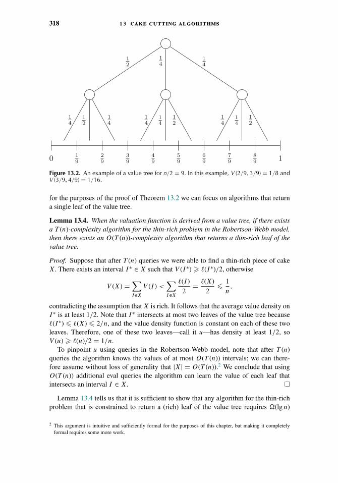
318 1 3 cake cutting algorithms
0 19
29
39
49
59
69
79
89 1
12
14
14
14
12
14
14
14
12
14
14
12
Figure 13.2. An example of a value tree for n/2 = 9. In this example, V (2/9, 3/9) = 1/8 andV (3/9, 4/9) = 1/16.
for the purposes of the proof of Theorem 13.2 we can focus on algorithms that returna single leaf of the value tree.
Lemma 13.4. When the valuation function is derived from a value tree, if there existsa T (n)-complexity algorithm for the thin-rich problem in the Robertson-Webb model,then there exists an O(T (n))-complexity algorithm that returns a thin-rich leaf of thevalue tree.
Proof. Suppose that after T (n) queries we were able to find a thin-rich piece of cakeX. There exists an interval I ∗ ∈ X such that V (I ∗) � (I ∗)/2, otherwise
V (X) =∑I∈X
V (I ) <∑I∈X
(I )
2= (X)
2� 1
n,
contradicting the assumption that X is rich. It follows that the average value density onI ∗ is at least 1/2. Note that I ∗ intersects at most two leaves of the value tree because (I ∗) � (X) � 2/n, and the value density function is constant on each of these twoleaves. Therefore, one of these two leaves—call it u—has density at least 1/2, soV (u) � (u)/2 = 1/n.
To pinpoint u using queries in the Robertson-Webb model, note that after T (n)queries the algorithm knows the values of at most O(T (n)) intervals; we can there-fore assume without loss of generality that |X| = O(T (n)).2 We conclude that usingO(T (n)) additional eval queries the algorithm can learn the value of each leaf thatintersects an interval I ∈ X.
Lemma 13.4 tells us that it is sufficient to show that any algorithm for the thin-richproblem that is constrained to return a (rich) leaf of the value tree requires �(lg n)
2 This argument is intuitive and sufficiently formal for the purposes of this chapter, but making it completelyformal requires some more work.

1 3 .4 complexity of cake cutting 319
queries. Intuitively, the path from the root to a rich leaf must have “many” heavy edges.To find out exactly how many, note that the height of the tree is H = log3(n/2) =θ(lg(n)). Denoting the number of heavy edges on the path from the root to a leaf u byq(u), we have
1
n� V (u) =
(1
2
)q(u) (1
4
)H−q(u)
=(
1
4
)H− q(u)2
.
It follows that 4H−q(u)/2 � n, and hence 2(H − q(u)/2) � lg n. Using the fact that2H − lg n = �(lg n) we conclude that q(u) = �(lg n). In other words, a constantfraction of the edges on the path to u must be heavy.
If the algorithm were only allowed to directly query the edges of the value tree, alower bound of �(lg n) would follow almost immediately from the preceding argument.Indeed, unqueried edges could be light, so the algorithm must query a constant fractionof the edges on the path from the root to a leaf in order to find a constant fraction ofheavy edges. However, we are interested in algorithms that operate in the Robertson-Webb model, so we must explain how to simulate cut and eval queries by revealingedges of the value tree.
We say that a node u is revealed if the weights of all edges of every node on the pathfrom the root to u are known to the algorithm. Intuitively the approach is to generouslyanswer the algorithm’s queries by revealing nodes in a way that provides at least asmuch information as requested. We note the following facts:
� If u is revealed, its value (formally, the value of the interval associated with the node)V (u) is known to the algorithm.
� If u = [x, y] is revealed then V (0, x) is known to the algorithm: Let u0, . . . , uk = u bethe path from the root to u, then V (0, x) is the sum of the values of the nodes to the leftof each ui , all of which are also revealed. Moreover, V (y, 1) = 1 − V (0, x) − V (x, y)is also known.
� If z ∈ [x, y] where [x, y] is a revealed leaf then V (0, z) can be computed, using thepreceding observation and the fact that V (x, z) = V (x, y) · ([x,z])
2/n.
� If w ∈ u, u is a revealed leaf, and α is a given cake value, then it is possible to compute theleast common ancestor of u and the leaf that contains the point z such that V (w, z) = α.Indeed, let u0, . . . , uH = u be the path from the root to the leaf u, and let yi be therightmost point of ui . We start from i = H and working our way upward iterativelycompute V (w, yi), where V (w, yH ) = ([w,yH ])
2/nand V (w, yi) is the sum of V (w, yi+1)
and the values of the children of ui to the right of ui+1. We return the first ui (i.e., theone with the largest index) such that V (w, yi) � α.
Proof of Theorem 13.2. It is sufficient to prove that any algorithm for the thin-richproblem that returns a leaf of the value tree requires �(lg n) queries. We will answerthe algorithm’s eval and cut queries by revealing nodes of the value tree in a way thatmaintains the following invariant: After k queries, there are at most 2k edges that areknown to be heavy on any path from the root to a leaf. Because we have shown that�(lg n) edges on the path must be known to be heavy, the theorem will directly follow.Initially the invariant trivially holds.
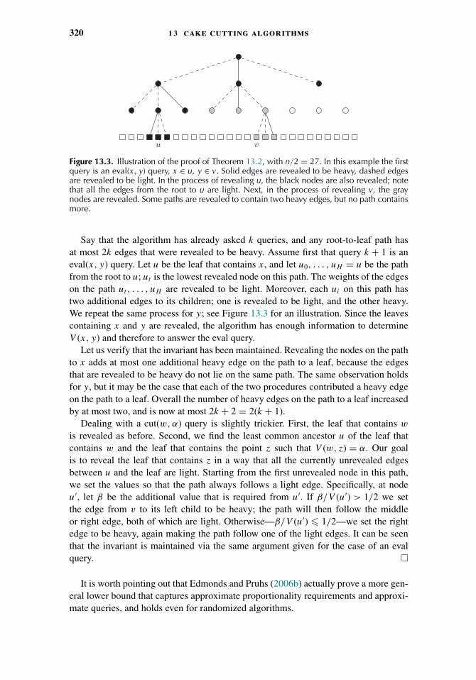
320 1 3 cake cutting algorithms
u v
Figure 13.3. Illustration of the proof of Theorem 13.2, with n/2 = 27. In this example the firstquery is an eval(x, y) query, x ∈ u, y ∈ v. Solid edges are revealed to be heavy, dashed edgesare revealed to be light. In the process of revealing u, the black nodes are also revealed; notethat all the edges from the root to u are light. Next, in the process of revealing v, the graynodes are revealed. Some paths are revealed to contain two heavy edges, but no path containsmore.
Say that the algorithm has already asked k queries, and any root-to-leaf path hasat most 2k edges that were revealed to be heavy. Assume first that query k + 1 is aneval(x, y) query. Let u be the leaf that contains x, and let u0, . . . , uH = u be the pathfrom the root to u; ut is the lowest revealed node on this path. The weights of the edgeson the path ut , . . . , uH are revealed to be light. Moreover, each ui on this path hastwo additional edges to its children; one is revealed to be light, and the other heavy.We repeat the same process for y; see Figure 13.3 for an illustration. Since the leavescontaining x and y are revealed, the algorithm has enough information to determineV (x, y) and therefore to answer the eval query.
Let us verify that the invariant has been maintained. Revealing the nodes on the pathto x adds at most one additional heavy edge on the path to a leaf, because the edgesthat are revealed to be heavy do not lie on the same path. The same observation holdsfor y, but it may be the case that each of the two procedures contributed a heavy edgeon the path to a leaf. Overall the number of heavy edges on the path to a leaf increasedby at most two, and is now at most 2k + 2 = 2(k + 1).
Dealing with a cut(w, α) query is slightly trickier. First, the leaf that contains w
is revealed as before. Second, we find the least common ancestor u of the leaf thatcontains w and the leaf that contains the point z such that V (w, z) = α. Our goalis to reveal the leaf that contains z in a way that all the currently unrevealed edgesbetween u and the leaf are light. Starting from the first unrevealed node in this path,we set the values so that the path always follows a light edge. Specifically, at nodeu′, let β be the additional value that is required from u′. If β/V (u′) > 1/2 we setthe edge from v to its left child to be heavy; the path will then follow the middleor right edge, both of which are light. Otherwise—β/V (u′) � 1/2—we set the rightedge to be heavy, again making the path follow one of the light edges. It can be seenthat the invariant is maintained via the same argument given for the case of an evalquery.
It is worth pointing out that Edmonds and Pruhs (2006b) actually prove a more gen-eral lower bound that captures approximate proportionality requirements and approxi-mate queries, and holds even for randomized algorithms.
1 3 .4 complexity of cake cutting 321
13.4.2 The Complexity of Envy-Free Cake Cutting
While the complexity of proportional cake cutting is well understood, envy-freenessis a completely different matter. The classic Selfridge-Conway algorithm provides anenvy-free solution for the case of three agents, but it took another three decades untiltheir algorithm was extended to any number of agents. The celebrated algorithm ofBrams and Taylor (1995) is a discrete envy-free cake cutting algorithm. When viewedthrough the Robertson-Webb lens, the algorithm can be simulated via eval and cutqueries, and is guaranteed to terminate—it is finite. But it does have a serious flaw: Itsrunning time is unbounded. Specifically, the analysis of the Dubins-Spanier and Even-Paz algorithms bounded the required number of queries as a function of the numberof agents: O(n2) and O(n lg n), respectively. In contrast, for any n � 4 and any k ∈ Nthere are valuation functions V1, . . . , Vn such that the Brams-Taylor algorithm requiresat least k queries to terminate.3
It is natural to ask whether the envy-free cake cutting problem is inherently diffi-cult: Is it provably impossible to design a bounded envy-free cake cutting algorithm?Currently there are two partial answers to this question. The first result restricts theallocations to be contiguous.
Theorem 13.5 (Stromquist, 2008). For any n � 3, there is no finite envy-free cake-cutting algorithm that outputs contiguous allocations.4
However, from a technical point of view the restriction to contiguous pieces issevere. Indeed, the Brams-Taylor algorithm is finite and guarantees an envy-free allo-cation for any number of agents. Moreover, for the case of n = 3 (which is captured byTheorem 13.5), the Selfridge-Conway algorithm is actually a bounded envy-free algo-rithm! Interestingly, the latter algorithm even allocates “almost contiguous” pieces, inthat the piece of each agent is the union of at most two intervals.
The second result does not make any assumptions, but achieves a relatively weaklower bound.
Theorem 13.6 (Procaccia, 2009). Any envy-free cake-cutting algorithm requires �(n2)queries in the Robertson-Webb model.
This theorem is somewhat unsatisfying, because the gap between �(n2) and“unbounded” is still, well, unbounded. Nevertheless, it does establish a separationbetween the O(n lg n) complexity of proportional cake cutting and the �(n2) complex-ity of envy-free cake cutting. In other words, the theorem implies that envy-freenessis provably harder than proportionality, and provides a partial explanation for whyenvy-freeness has been so elusive.
The running time of the Brams-Taylor algorithm depends on the valuation functions;this fact seems to suggest that the hardness of envy-free cake cutting draws on thepossible richness of the valuation functions. This turns out not to be the case: In theRobertson-Webb model, envy-free cake cutting is equally hard when the valuationfunctions are piecewise uniform.
3 Even when moving knives are allowed, there are no known bounded solutions beyond the case of n = 5 (Bramset al., 1997b; Saberi and Wang, 2009).
4 This theorem was extended by Deng et al. (2012).
322 1 3 cake cutting algorithms
Theorem 13.7 (Kurokawa et al., 2013). Suppose there is an algorithm that computesan envy-free allocation for n agents with piecewise uniform valuations using at mostf (n) queries in the Robertson-Webb model. Then the algorithm can compute an envy-free allocation for n agents with general valuation functions using at most f (n) queries.
Proof. Let V1, . . . , Vn be general valuation functions. We let the algorithm interactwith these functions via cut and eval queries. Suppose first that the algorithm outputsan allocation A using at most f (n) queries. Our goal is to construct piecewise uniformvaluation functions U1, . . . , Un that lead to an identical interaction with the algorithm,and identical values for the allocated pieces (i.e., Vi(Ai) = Ui(Ai) for all i ∈ N ). Sincethe algorithm is guaranteed to output an envy-free allocation with respect to U1, . . . , Un,these properties would imply that A is envy-free with respect to the general valuationfunctions V1, . . . , Vn.
To construct the valuation functions U1, . . . , Un, we define sets of points Mi asfollows. First, Mi contains all “marks” made during the algorithm’s interaction withagent i; an evali(x, y) query marks the points x and y, and a cuti(x, α) query marksthe point x and the point y that is returned. Second, for each j ∈ N and each interval[x, y] ∈ Aj , Mi contains x and y; in other words, the allocation A induces a partitionof [0, 1] into subintervals, and Mi contains the boundaries of these intervals. Third, Mi
contains the boundaries of the cake, 0 and 1.Let Mi = {0 = xi1, xi2, . . . , xiki
= 1}, where xit < xi,t+1 for all t = 1, . . . , ki − 1.Let μi = maxt
Vi (xit ,xi,t+1)xi,t+1−xit
be the maximum average density on any interval defined bythe points in Mi . The valuation function Ui is induced by a piecewise uniform valuedensity function ui , defined as follows:
ui(x) ={
μi ∃t s.t. x ∈[xi,t+1 − Vi (xit ,xi,t+1)
μi, xi,t+1
]0 otherwise.
For all i ∈ N and t = 1, . . . , ki − 1 it holds that
Ui(xit , xi,t+1) = Vi(xit , xi,t+1)
μi
· μi = Vi(xit , xi,t+1).
Since the boundaries of intervals in each Aj are contained in Mi (i.e., they areamong the points xit ), it follows that for every i, j ∈ N , Ui(Aj ) = Vi(Aj ). We alsoclaim that the algorithm’s interaction with U1, . . . , Un is identical to its interactionwith V1, . . . , Vn. Indeed, the answers to evali queries are identical because the marksmade by the query are contained in the set Mi . To see that the answers to cuti queriesare also identical, consider a cuti(x, α) = y query. Note that Ui(x, y) = Vi(x, y) = α
because x, y ∈ Mi , and crucially for any ε > 0, Ui(x, y − ε) < α because ui is strictlypositive in the left neighborhood of y. This concludes the proof under the assumptionthat the algorithm terminates after at most f (n) queries.
If the algorithm does not terminate after f (n) queries, consider the first f (n) queries,and repeat the process of constructing U1, . . . , Un without including the boundariesof allocated intervals in M1, . . . , Mn. As before, the algorithm’s interaction withU1, . . . , Un is identical to its interaction with V1, . . . , Vn, and thus the assumptionthat the algorithm proceeds to query f (n) + 1 contradicts the assumption that thenumber of queries is bounded by f (n) given piecewise uniform valuations.

1 3 .5 optimal cake cutting 323
Theorem 13.7 has two complementary interpretations. On one hand, the theoremtells us that to design an envy-free algorithm we can focus on handling the seeminglysimple case of piecewise uniform valuations. On the other hand, if one seeks to prove alower bound for envy-free cake cutting, the theorem implies that constructing elaboratevaluation functions would not be a fruitful approach.
In order to conclude this section on a positive note, we next relax the envy-freenessrequirement, instead asking for ε-envy-freeness: Vi(Ai) � Vi(Aj ) − ε for all i, j ∈ N .Despite the difficulties we have discussed, it turns out that this natural relaxation canbe solved by a very simple, computationally efficient algorithm. First, the algorithmasks each agent i ∈ N to cut the cake into %1/ε& disjoint intervals worth ε each (exceptfor maybe the rightmost interval, which is worth at most ε); this step requires roughlyn/ε cut queries. Next the algorithm sorts the cut points made by all the agents, and askseach agent to evaluate each interval between two adjacent cut points; this step requiresroughly n2/ε eval queries.
We claim that at this point the algorithm has sufficient information to computean ε-envy-free allocation. Indeed, we can treat the intervals between adjacent cutpoints as indivisible goods where, crucially, each good is worth at most ε to anyagent. The goods are allocated in a round-robin fashion: each of the agents 1, 2, . . . , n
selects its most preferred good in that order, and we repeat this process until all thegoods have been selected. To see why this allocation is ε-envy-free consider an agenti ∈ N , and consider the sequence of choices starting from the first time i selected agood: i, i + 1, . . . , n, 1, . . . , i − 1, i, . . . , i − 1, . . . In each subsequence i, . . . , i − 1,i prefers its own good to the goods selected by other agents. The only potential sourceof envy is the selections made by agents 1, . . . , i − 1 before i first selected a good, butthese agents received one good each in this phase, and Vi(g) � ε for each good g.
13.5 Optimal Cake Cutting
So far we were interested in algorithms that achieve fairness guarantees. But if weare also interested in economic efficiency, better allocations may be achieved at theexpense of depriving some agents of their fair share.
To quantify the efficiency of an allocation A we employ the notion of social wel-fare. While this notion has several interpretations, the computer science literaturetypically adopts the utilitarian interpretation, as do we: The social welfare of A issw(A) = ∑
i∈N Vi(Ai). It is important to note that this notion assumes the agents havecomparable valuation functions. Although earlier we have assumed that Vi(0, 1) = 1,the assumption was made for ease of exposition; proportionality and envy-freenessinvolve inequalities that only constrain the valuation function of a single agent; thatis, two valuation functions never appear in the same inequality. In contrast, whendiscussing social welfare our objective is the sum of all valuation functions, so ourassumption that Vi(0, 1) = 1 for all i ∈ N takes a more literal interpretation.
13.5.1 Computation of Optimal Fair Allocations
Our next task is the computation of optimal fair allocations; that is, we wish to maxi-mize social welfare under fairness constraints. To circumvent the computational issues
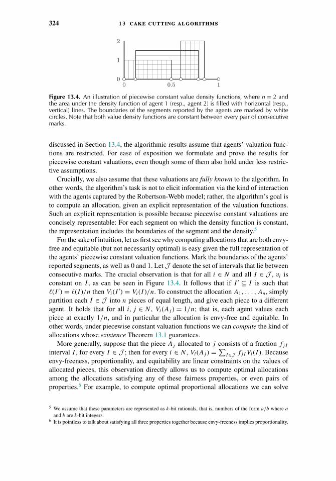
324 1 3 cake cutting algorithms
0 0.5 10
1
2
Figure 13.4. An illustration of piecewise constant value density functions, where n = 2 andthe area under the density function of agent 1 (resp., agent 2) is filled with horizontal (resp.,vertical) lines. The boundaries of the segments reported by the agents are marked by whitecircles. Note that both value density functions are constant between every pair of consecutivemarks.
discussed in Section 13.4, the algorithmic results assume that agents’ valuation func-tions are restricted. For ease of exposition we formulate and prove the results forpiecewise constant valuations, even though some of them also hold under less restric-tive assumptions.
Crucially, we also assume that these valuations are fully known to the algorithm. Inother words, the algorithm’s task is not to elicit information via the kind of interactionwith the agents captured by the Robertson-Webb model; rather, the algorithm’s goal isto compute an allocation, given an explicit representation of the valuation functions.Such an explicit representation is possible because piecewise constant valuations areconcisely representable: For each segment on which the density function is constant,the representation includes the boundaries of the segment and the density.5
For the sake of intuition, let us first see why computing allocations that are both envy-free and equitable (but not necessarily optimal) is easy given the full representation ofthe agents’ piecewise constant valuation functions. Mark the boundaries of the agents’reported segments, as well as 0 and 1. Let J denote the set of intervals that lie betweenconsecutive marks. The crucial observation is that for all i ∈ N and all I ∈ J , vi isconstant on I , as can be seen in Figure 13.4. It follows that if I ′ ⊆ I is such that (I ′) = (I )/n then Vi(I ′) = Vi(I )/n. To construct the allocation A1, . . . , An, simplypartition each I ∈ J into n pieces of equal length, and give each piece to a differentagent. It holds that for all i, j ∈ N , Vi(Aj ) = 1/n; that is, each agent values eachpiece at exactly 1/n, and in particular the allocation is envy-free and equitable. Inother words, under piecewise constant valuation functions we can compute the kind ofallocations whose existence Theorem 13.1 guarantees.
More generally, suppose that the piece Aj allocated to j consists of a fraction fjI
interval I , for every I ∈ J ; then for every i ∈ N , Vi(Aj ) = ∑I∈J fjIVi(I ). Because
envy-freeness, proportionality, and equitability are linear constraints on the values ofallocated pieces, this observation directly allows us to compute optimal allocationsamong the allocations satisfying any of these fairness properties, or even pairs ofproperties.6 For example, to compute optimal proportional allocations we can solve
5 We assume that these parameters are represented as k-bit rationals, that is, numbers of the form a/b where a
and b are k-bit integers.6 It is pointless to talk about satisfying all three properties together because envy-freeness implies proportionality.
1 3 .5 optimal cake cutting 325
the following linear program (Cohler et al., 2011):
maxn∑
i=1
∑I∈J
fiIVi(I ), (13.1)
s.t.n∑
i=1
fiI � 1 ∀I ∈ J , (13.2)
∑I∈J
fiIVi(I ) � 1
n∀i ∈ N, (13.3)
fiI � 0 ∀i ∈ N, I ∈ J . (13.4)
The social welfare objective is formulated as Equation 13.1. Equation 13.2 ensuresthat the fractions of interval I that are allocated sum up to at most 1, and Equation 13.4guarantees that these fractions are nonnegative. The proportionality constraint is for-mulated as Equation (13.3).
In contrast, as in Section 13.4 (cf. Theorem 13.5), when contiguous allocations arerequired the problem becomes much harder.
Theorem 13.8 (Bei et al., 2012). Given explicit piecewise constant valuation functionsand assuming that the allocation must be proportional and contiguous, the optimalsocial welfare is NP-hard to approximate to a factor of �(
√n).
13.5.2 The Price of Fairness
The results of Section 13.5.1 enable the computation of optimal fair allocations; buthow good are these allocations? The fairness constraints cause a degradation in socialwelfare, which can be measured using the price of fairness. The price of proportionality(resp., envy-freeness, equitability) is the worst-case (over agents’ valuation functions)ratio between the social welfare of the optimal allocation, and the social welfare of theoptimal proportional (resp., envy-free, equitable) allocation.
Theorem 13.9 (Caragiannis et al., 2009). The price of proportionality is �(√
n).
To establish the upper bound, we must show that for any collection of valuationfunctions, the ratio between the social welfare of the optimal allocation and the opti-mal proportional allocation is O(
√n). The lower bound only requires producing one
example of valuation functions such that this ratio is �(√
n).
Proof of Theorem 13.9. To prove the upper bound, let V1, . . . , Vn be the agents’ valua-tion functions, and let A∗ be the optimal allocation. Let L = {i ∈ N : Vi(A∗
i ) � 1/√
n}be the set of “large” agents, and S = N \ L be the set of “small” agents. We considertwo cases.
Case 1: |L| � √n. It follows from the assumption that |S| � n −√
n. Define anallocation A as follows. For each i ∈ S, reallocate A∗
i among the agents in S so thatfor each j ∈ S, Vj (Aj ∩ A∗
i ) � Vj (A∗i )/|S|; this can even be done algorithmically
(although only existence is required), for example, using (a slight variation of) the

326 1 3 cake cutting algorithms
Even-Paz protocol. For each i ∈ L, we reallocate A∗i among the agents in {i} ∪ S so
that
Vi(Ai ∩ A∗i ) �
√n · Vi(A∗
i )√n + |S| ,
and for all j ∈ S,
Vj (Aj ∩ A∗i ) � Vj (A∗
i )√n + |S| .
This can be done, for example, by creating√
n − 1 copies of agent i with identicalvaluations and running the Even-Paz algorithm with the
√n identical agents and the
agents in S.Note that the allocation A1, . . . , An is proportional, because for all i ∈ L,
Vi(Ai) �√
n · Vi(A∗i )√
n + |S| �1√
n + |S| �1
n,
and for all i ∈ S,
Vi(Ai) �∑j∈L
Vi(A∗j )√
n + |S| +∑j∈S
Vi(A∗j )
|S| �∑
j∈N Vi(A∗j )
n= 1
n.
Moreover, for each i ∈ N , Vi(Ai) � Vi(A∗i )/
√n, hence it holds that sw(A) �
sw(A∗)/√
n; the ratio is at most√
n.Case 2: |L| <
√n. Observe that sw(A∗) � |L| + |S|/√n < 2
√n, while for any
proportional allocation A, sw(A) �∑i∈N 1/n = 1; the ratio is O(
√n).
To establish the lower bound, consider the following valuation functions. The setof agents L ⊆ N now contains exactly
√n agents, each uniformly interested only in
a single interval of length 1/√
n, such that for i, j ∈ L the two desired intervals aredisjoint. The set of agents S = N \ L contains n −√
n agents that desire the entirecake uniformly.
The optimal allocation A∗ gives each agent in L its desired interval, hence sw(A∗) =√n. In contrast, any proportional allocation A would have to give an interval of length
1/n to each agent in S, leaving only 1/√
n by length to the agents in L. With theirdensity of
√n, it must hold that
∑i∈L Vi(Ai) �
√n/
√n = 1, while
∑i∈S Vi(Ai) � 1.
Thus, sw(A) � 2; the ratio is �(√
n).
Two comments on the theorem and its proof are in order. First, the lower bound of�(
√n) also applies to the price of envy-freeness, because every envy-free allocation is
proportional. However, no nontrivial o(n) upper bound on the price of envy-freenessis known. Second, the valuation functions used in the lower bound construction arepiecewise uniform, so one cannot hope to circumvent this negative result by restrictingthe valuation functions. It is not hard to see that a similar construction only admitsseverely suboptimal equitable allocations, and indeed the price of equitability is steep.
Theorem 13.10 (Caragiannis et al., 2009). The price of equitability is �(n).
While the price of equitability is significantly higher than the price of proportionality,the comparison relies on a worst-case notion, and it could be the case that there areinstances where the optimal equitable allocation is superior to the optimal proportional
1 3 .5 optimal cake cutting 327
allocation in terms of social welfare. The last technical result for this chapter rulesout this situation, even if we replace proportionality by the stronger envy-freenessrequirement; for ease of exposition we formulate and prove the theorem for piecewiseconstant valuations.
Theorem 13.11 (Brams et al., 2012a). Given piecewise constant valuation functionsV1, . . . , Vn, let A∗ be the optimal equitable allocation and let A∗∗ be the optimalenvy-free allocation. Then sw(A∗) � sw(A∗∗).
The theorem’s proof draws on a connection between cake cutting and linear Fishermarkets. Instead of a single heterogeneous divisible good, the market includes a setG = {1, . . . , m} of homogeneous divisible goods. The utility of good j for agent i isdenoted by uij . An allocation gives each agent i ∈ N a fraction fij of good j such thatfor all j ∈ G,
∑i∈N fij � 1. The utility of agent i for an allocation is
∑j∈G fijuij .
Consider a cake allocation A, and let the set of goods be the pieces in A, that is, goodj corresponds to the piece Aj , and uij = Vi(Aj ). We claim that given an allocationf = (fij )i∈N,j∈G in the Fisher market, there is an allocation A′ in the correspondingcake cutting setting such that Vi(A′
j ) = ∑k∈G fjkuik for all i, j ∈ N ; that is, agents’
utilities in the Fisher market can be replicated in the cake cutting setting. This claimcan be established via similar arguments to the ones we have seen in Section 13.5.1:Each piece Aj is divides into intervals such that each interval is valued uniformly byall agents, and then an fij -fraction (by length) of each of these intervals is added to thepiece A′
i .
Lemma 13.12 (see, e.g., Vazirani, 2007). Consider a linear Fisher market whereagent i ∈ N has budget ei ,
∑i∈N ei = 1, and for every j ∈ G there is i ∈ N such that
uij > 0. Then there exists a price vector p = (p1, . . . , pm) such that pj > 0 for allj ∈ G and
∑j∈G pj = 1, and an allocation f such that:
1. Goods are fully allocated: For all j ∈ G,∑
i∈N fij = 1.2. Agents only get their most profitable goods under the price vector p: For all i ∈ N, j ∈
G, if fij > 0 then j ∈ argmaxk∈Guik/pk .3. Agents spend their entire budgets: For all i ∈ N ,
∑j∈G fijpj = ei .
Proof of Theorem 13.11. Consider the optimal equitable allocation A∗. We constructa linear Fisher market where good j corresponds to A∗
j , and uij = Vi(A∗j ). We also
set the agents’ budgets to be identical: ei = 1/n for all i ∈ N . Using Lemma 13.12we obtain an allocation f in the Fisher market satisfying properties 1–3. Construct anallocation A that corresponds to the Fisher market allocation, as explained earlier. Weclaim that A is an envy-free allocation and sw(A) � sw(A∗).
The envy-freeness of A follows directly from the assumptions that the price of eachagent’s bundle is exactly 1/n and each agent receives only items that maximize theratio of utility to price. Formally, for an agent i ∈ N let r∗i = maxj∈G uij /pj ; then
Vi(Ai) =∑j∈G
fijuij =∑j∈G
fij
uij
pj
pj =∑j∈G
fij r∗i pj = r∗i
n, (13.5)
328 1 3 cake cutting algorithms
where the third transition follows from the second property in Lemma 13.12, and thefourth transition follows from the third property and ei = 1/n. Likewise,
Vi(Ak) =∑j∈G
fkjuij =∑j∈G
fkj
uij
pj
pj �∑j∈G
fkj r∗i pj = r∗i
n.
Next we prove that sw(A) � sw(A∗). Because A∗ is equitable there exists α > 0 suchthat Vi(A∗
i ) = α for all i ∈ N ; hence sw(A∗) = nα. We also know from Equation (13.5)that sw(A) = 1
n
∑i∈N r∗i . By definition, r∗i � uii/pi ; recall that uii = Vi(A∗
i ) = α. Weconclude that
sw(A) = 1
n
∑i∈N
r∗i � 1
n
∑i∈N
uii
pi
= α
n
∑i∈N
1
pi
� α
nn2 = nα = sw(A∗),
where the fourth transition holds because∑
i∈N pi = 1, and therefore the sum∑i∈N (1/pi) is minimized when pi = 1/n for all i ∈ N .
13.6 Bibliography and Further Reading
Section 13.4 covers complexity results due to Edmonds and Pruhs (2006b), Stromquist(2008), Procaccia (2009), and Kurokawa et al. (2013). The result of Stromquist (2008)was generalized by Deng et al. (2012). Other papers on the complexity of cake cuttinginclude the ones by Woeginger and Sgall (2007), Magdon-Ismail et al. (2003), andBalkanski et al. (2014). A beautiful paper by Edmonds and Pruhs (2006a) circumventsTheorem 13.2 by designing a randomized, approximately proportional algorithm thatrequires only O(n) queries in the Robertson-Webb model.
Section 13.5 includes results by Caragiannis et al. (2009), Cohler et al. (2011),Brams et al. (2012a), and Bei et al. (2012); all of these papers contain numerous resultsthat are not covered here. The complexity of cake cutting with contiguous pieces butwithout fairness constraints is explored by Aumann et al. (2013). The price of fairnesswas independently proposed by Caragiannis et al. (2009) and Bertsimas et al. (2011);the concept is inspired by the price of stability (Anshelevich et al., 2004). Aumannand Dombb (2010) study the price of fairness under the restriction that allocationsare contiguous. Arzi et al. (2011) show that (when pieces are contiguous) the optimalfair allocation can actually be better if a piece of cake is discarded, and quantifythe potential benefit. It is also worth mentioning that the problem of interpersonalcomparison of utility has been extensively debated by philosophers and economists;for more information see the survey by Hammond (1991).
This chapter does not attempt to cover game-theoretic issues in cake cutting. Asimple randomized strategyproof, envy-free algorithm was independently discoveredby Chen et al. (2013) and Mossel and Tamuz (2010). Chen et al. (2013) also design amore intricate deterministic strategyproof envy-free algorithm for piecewise uniformvaluation functions, which is generalized by Aziz and Ye (2014); under the sameassumption, Maya and Nisan (2012) give a characterization of strategyproof, Pareto-efficient cake cutting algorithms. Nash equilibria of cake cutting algorithms are studiedby Nicolo and Yu (2008) and Branzei and Miltersen (2013).
acknowledgments 329
This chapter also avoids nonconstructive existence results, focusing on algorithmicresults instead. The book by Barbanel (2005) is a good source of information aboutexistence results in fair division.
Additional cake cutting research has recently explored a variety of questions. Forexample, Brams et al. (2013) show that Pareto-efficient, envy-free, and equitable allo-cations may not exist when n � 3; Lindner and Rothe (2009) aim to design algorithmsthat provide guarantees with respect to the number of envy relations between pairsof agents; Zivan (2011) establishes a trade-off between the strength of proportionalityguarantees (which he interprets as the level of trust between agents) and social welfare;Caragiannis et al. (2011) investigate the approximate fairness guarantees that can beachieved when agents’ valuation functions are nonadditive; and Branzei et al. (2013a)study externalities in cake cutting.
In a recent paper, Ghodsi et al. (2011) suggested that fair division theory can beapplied to the problem of allocating computational resources (e.g., CPU, RAM) incluster computing environments. Users are modeled as having Leontief preferences,meaning that they demand the resources in fixed proportions. While the model issomewhat different, it has much in common with the cake cutting model. Other papersthat study this research direction include papers by Dolev et al. (2012), Gutman andNisan (2012), Parkes et al. (2014), and Kash et al. (2014).
Acknowledgments
The author thanks Yair Dombb and Eric Pacuit for their very helpful reviews of thischapter. The author is partially supported by the National Science Foundation undergrants CCF-1215883 and IIS-1350598.


PART III
Coalition Formation


CHAPTER 14
Matching under Preferences
Bettina Klaus, David F. Manlove, and Francesca Rossi
14.1 Introduction and Discussion of Applications
Matching theory studies how agents and/or objects from different sets can be matchedwith each other while taking agents’ preferences into account. The theory originatedin 1962 with a celebrated paper by David Gale and Lloyd Shapley (1962), in whichthey proposed the Stable Marriage Algorithm as a solution to the problem of two-sidedmatching. Since then, this theory has been successfully applied to many real-worldproblems such as matching students to universities, doctors to hospitals, kidney trans-plant patients to donors, and tenants to houses. This chapter will focus on algorithmicas well as strategic issues of matching theory.
Many large-scale centralized allocation processes can be modelled by matchingproblems where agents have preferences over one another. For example, in China, over10 million students apply for admission to higher education annually through a cen-tralized process. The inputs to the matching scheme include the students’ preferencesover universities, and vice versa, and the capacities of each university.1 The task is toconstruct a matching that is in some sense optimal with respect to these inputs.
Economists have long understood the problems with decentralized matching mar-kets, which can suffer from such undesirable properties as unravelling, congestionand exploding offers (see Roth and Xing, 1994, for details). For centralized markets,constructing allocations by hand for large problem instances is clearly infeasible. Thuscentralized mechanisms are required for automating the allocation process.
Given the large number of agents typically involved, the computational efficiencyof a mechanism’s underlying algorithm is of paramount importance. Thus we seekpolynomial-time algorithms for the underlying matching problems. Equally importantare considerations of strategy: an agent (or a coalition of agents) may manipulatetheir input to the matching scheme (e.g., by misrepresenting their true preferences orunderreporting their capacity) in order to try to improve their outcome. A desirable
1 In fact, students are first assigned to universities and then to their programme of study within the university(see, e.g., Zhu, 2014).
333
334 1 4 matching under preferences
property of a mechanism is strategyproofness, which ensures that it is in the bestinterests of an agent to behave truthfully.
The study of matching problems involving preferences was begun in 1962 with theseminal paper of Gale and Shapley (1962) who gave an efficient algorithm for theso-called Stable Marriage problem (which involves matching men to women based oneach person having preferences over members of the opposite sex) and showed howto extend it to the College Admissions problem, a many-to-one extension of the StableMarriage problem which involves allocating students to colleges based on collegecapacities, as well as on students’ preferences over colleges, and vice versa. Theiralgorithm has come to be known as the Gale–Shapley algorithm.
Since 1962, the study of matching problems involving preferences has grown intoa large and active research area, and numerous contributions have been made by com-puter scientists, economists, and mathematicians, among others. Several monographsexclusively dealing with this class of problems have been published (Knuth, 1976;Gusfield and Irving, 1989; Roth and Sotomayor, 1990; Manlove, 2013).
A particularly appealing aspect of this research area is the range of practical appli-cations of matching problems, leading to real-life scenarios where efficient algorithmscan be deployed and issues of strategy can be overcome. One of the best-known exam-ples is the National Resident Matching Program (NRMP) in the United States, whichhandles the annual allocation of intending junior doctors (or residents) to hospital posts.In 2014, 40,394 aspiring junior doctors applied via the NRMP for 29,671 availableresidency positions (NRMP, 2014). The problem model is very similar to Gale andShapley’s College Admissions problem, and indeed an extension of the Gale–Shapleyalgorithm is used to construct the allocation each year (Roth, 1984a; Roth and Peran-son, 1997). Similar medical matching schemes exist in Canada, Japan, and the UnitedKingdom. As Roth argued, the key property for a matching to satisfy in this context isstability, which ensures that a resident and hospital do not have the incentive to deviatefrom their allocation and become matched to one another.
Similar applications arise in the context of School Choice (Abdulkadiroglu andSonmez, 2003). For example in Boston and New York, centralized matching schemesare employed to assign pupils to schools on the basis of the preferences of pupils (ormore realistically their parents) over schools, and pupils’ priorities for assignment toa given school (Abdulkadiroglu et al., 2005a, 2005b). A school’s priority for a pupilmight include issues such as geographical proximity and whether the pupil has a siblingat the school already, among others.
Kidney exchange (Roth et al., 2004, 2005) is another application of matching thathas grown in importance in recent years. Sometimes, a kidney patient with a willingbut incompatible donor can swap their donor with that of another patient in a similarposition. Efficient algorithms are required to organize kidney “swaps” on the basis ofinformation about donor and patient compatibilities. Such swaps can involve two ormore patient–donor pairs, but usually the maximum number of pairs involved is three.Also altruistic donors can trigger “chains” involving swaps between patient–donorpairs. These allow for a larger number of kidney transplants (compared to those onecould perform based on deceased donors only) and thus more lives saved. Centralizedclearinghouses for kidney exchange are in operation on a nationwide scale in a number

1 4 .1 introduction and discussion of applications 335
of countries including the United States (Roth et al., 2004, 2005; Ashlagi and Roth,2012), the Netherlands (Keizer et al., 2005), and the United Kingdom (Johnson et al.,2008). The problem of maximizing the number of kidney transplants performed throughcycles and chains is NP-hard (Abraham et al., 2007a), though algorithms based onMixed Integer Programming have been developed and are used to solve this problemat scale in the countries mentioned (Abraham et al., 2007a; Dickerson et al., 2013;Manlove and O’Malley, 2012; Glorie et al., 2014).
The importance of the research area in both theoretical and practical senses wasunderlined in 2012 by the award of the Sveriges Riksbank Prize in Economic Sciences inMemory of Alfred Nobel (commonly known as the Nobel Prize in Economic Sciences)to Alvin Roth and Lloyd Shapley for their work in “the theory of stable allocations andthe practice of market design.” This reflects both Shapley’s contribution to the StableMarriage algorithm among other theoretical advances, and Roth’s application of theseresults to matching markets involving the assignment of junior doctors to hospitals,pupils to schools, and kidney patients to donors. The Nobel prize rules state that theprize cannot be awarded posthumously and hence David Gale (1921–2008) could notbe honoured for his important contributions.
Matching problems involving preferences can be classified as being either bipartiteor nonbipartite. In the former case, the agents are partitioned into two disjoint setsA and B, and the members of A have preferences over only the members of B (andpossibly vice versa). In the latter case we have one single set of agents, each of whomranks some or all of the others in order of preference. For space reasons we will consideronly bipartite matching problems involving preferences in this chapter.
Bipartite problems can be further categorized according to whether the preferencesare two-sided or one-sided. In the former case, members of both of the sets A and B
have preferences over one another, whereas in the latter case only the members of A
have preferences (over the members of B). Bipartite matching problems with two-sidedpreferences arise in the context of assigning junior doctors to hospitals, for example,while one-sided preferences arise in applications including the assignment of studentsto campus housing and reviewers to conference papers.
Our treatment covers ordinal preferences (where preferences are expressed in termsof first choice, second choice, etc.) rather than cardinal utilities (where preferencesare expressed in terms of real-numbered valuations). In their simplest form, modelsof kidney exchange problems can involve dichotomous preferences (a special case ofordinal preferences, where an agent either finds another agent acceptable or not, andis indifferent among those it does find acceptable), on the basis of whether a patient iscompatible with a potential donor. However, in practice, models of kidney exchange aremore complex, typically involving cardinal utilities rather than ordinal preferences, andtherefore the matching problems defined in this chapter do not encompass theoreticalmodels of kidney exchange.
The problems considered in this chapter sit strongly within the field of computationalsocial choice. This field lies at the interface of economics and computer science, andour approach will involve interleaving key aspects that have hitherto been consideredby the two communities in bodies of literature that have largely pertained to thetwo disciplines separately. Such key considerations involve the existence of structural
336 1 4 matching under preferences
results and efficient algorithms, and the derivation of strategyproof mechanisms. Thesetopics will be reviewed in each of the cases of bipartite matching problems with two-sided and one-sided preferences. Although space restrictions have necessarily limitedour coverage, we have tried to include the results that we feel will be of most importanceto the readership of this handbook.
The structure of this chapter is as follows. In Section 14.2, we focus on bipartitematching problems where both sides have preferences. Here the most important prop-erty for a matching to satisfy is stability. In Section 14.2.1 we define the key matchingproblems in this class, most notably the Hospitals / Residents problem, and we alsodefine stability in this context. We then state fundamental structural and algorithmicresults concerning the existence, computation, and structural properties of stable match-ings, in Section 14.2.2. Issues of strategy, and in particular the existence (or otherwise)of strategyproof mechanisms, are dealt with in Section 14.2.3. Next, in Section 14.2.4,we outline some further algorithmic results, including decentralized algorithms forcomputing stable matchings, variants of the Hospitals/Residents problem involvingties and couples, and many-to-many extensions.
Bipartite matching problems where only one side of the market has preferencesare considered in Section 14.3. The fundamental problems in this class are the HouseAllocation problem and its extension to Housing Markets. We define these problemstogether with key properties of matchings, including Pareto optimality and membershipof the core, in Section 14.3.1. Section 14.3.2 describes some important mechanismsthat can be used to produce Pareto optimal matchings and matchings in the core.Strategyproofness is considered in Section 14.3.3, and then further algorithmic resultsare described in Section 14.3.4, including the computation of maximum Pareto optimal,popular, and profile-based optimal matchings.
Finally, in Section 14.4 we give some concluding remarks and list some furthersources of reading.
14.2 Two-Sided Preferences
14.2.1 Introduction and Preliminary Definitions
The Hospitals/Residents problem2 (hr) (Gale and Shapley, 1962; Gusfield and Irving,1989; Roth and Sotomayor, 1990; Manlove, 2008) was first defined by Gale andShapley in their seminal paper “College Admissions and the Stability of Marriage”(Gale and Shapley, 1962).
An instance I of hr involves a set R = {r1, . . . , rn1} of residents and a setH = {h1, . . . , hn2} of hospitals. Each hospital hj ∈ H has a positive integer capac-ity, denoted by cj , indicating the number of posts that hj has. Also there is aset E ⊆ R × H of acceptable resident–hospital pairs. Let m = |E|. Each residentri ∈ R has an acceptable set of hospitals A(ri), where A(ri) = {hj ∈ H : (ri, hj ) ∈ E}.Similarly each hospital hj ∈ H has an acceptable set of residents A(hj ), whereA(hj ) = {ri ∈ R : (ri, hj ) ∈ E}.
2 The Hospitals/Residents problem is sometimes referred to as the College (or University or Stable) Admissionsproblem, or the Stable Assignment problem.
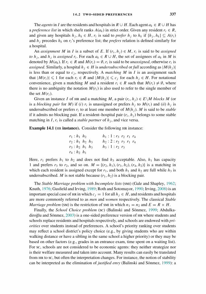
1 4 .2 two-sided preferences 337
The agents in I are the residents and hospitals in R ∪ H . Each agent ak ∈ R ∪ H hasa preference list in which she/it ranks A(ak) in strict order. Given any resident ri ∈ R,and given any hospitals hj , hk ∈ H , ri is said to prefer hj to hk if {hj , hk} ⊆ A(ri)and hj precedes hk on ri’s preference list; the prefers relation is defined similarly fora hospital.
An assignment M in I is a subset of E. If (ri, hj ) ∈ M , ri is said to be assignedto hj , and hj is assigned ri . For each ak ∈ R ∪ H , the set of assignees of ak in M isdenoted by M(ak). If ri ∈ R and M(ri) = ∅, ri is said to be unassigned, otherwise ri isassigned. Similarly, a hospital hj ∈ H is undersubscribed or full according as |M(hj )|is less than or equal to cj , respectively. A matching M in I is an assignment suchthat |M(ri)| � 1 for each ri ∈ R and |M(hj )| � cj for each hj ∈ H . For notationalconvenience, given a matching M and a resident ri ∈ R such that M(ri) �= ∅, wherethere is no ambiguity the notation M(ri) is also used to refer to the single member ofthe set M(ri).
Given an instance I of hr and a matching M , a pair (ri, hj ) ∈ E\M blocks M (oris a blocking pair for M) if (i) ri is unassigned or prefers hj to M(ri) and (ii) hj isundersubscribed or prefers ri to at least one member of M(hj ). M is said to be stableif it admits no blocking pair. If a resident–hospital pair (ri, hj ) belongs to some stablematching in I , ri is called a stable partner of hj , and vice versa.
Example 14.1 (hr instance). Consider the following hr instance:
r1 : h1 h2 h1 : 1 : r3 r2 r1 r4
r2 : h1 h2 h3 h2 : 2 : r2 r3 r1 r4
r3 : h2 h1 h3 h3 : 1 : r2 r3
r4 : h2 h1
Here, r1 prefers h1 to h2 and does not find h3 acceptable. Also, h1 has capacity1 and prefers r3 to r2, and so on. M = {(r2, h1), (r3, h2), (r4, h2)} is a matching inwhich each resident is assigned except for r1, and both h1 and h2 are full while h3 isundersubscribed. M is not stable because (r1, h2) is a blocking pair.
The Stable Marriage problem with Incomplete lists (smi) (Gale and Shapley, 1962;Knuth, 1976; Gusfield and Irving, 1989; Roth and Sotomayor, 1990; Irving, 2008) is animportant special case of hr in which cj = 1 for all hj ∈ H , and residents and hospitalsare more commonly referred to as men and women respectively. The classical StableMarriage problem (sm) is the restriction of smi in which n1 = n2 and E = R × H .
Finally, the School Choice problem (sc) (Balinski and Sonmez, 1999; Abdulka-diroglu and Sonmez, 2003) is a one-sided preference version of hr where students andschools replace residents and hospitals respectively, and schools are endowed with pri-orities over students instead of preferences. A school’s priority ranking over studentsmay reflect a school district’s policy choice (e.g., by giving students who are withinwalking distance or have a sibling in the same school a higher priority) or they may bebased on other factors (e.g., grades in an entrance exam, time spent on a waiting list).For sc, schools are not considered to be economic agents: they neither strategize noris their welfare measured and taken into account. Many results can easily be translatedfrom hr to sc, but often the interpretation changes. For instance, the notion of stabilitycan be interpreted as the elimination of justified envy (Balinski and Sonmez, 1999): a

338 1 4 matching under preferences
student can justifiably envy the assignment of another student to a school if he likesthat school better than his own assignment and he has a higher priority (with a lowerpriority, envy might be present as well but is not justifiable). Two recent and exhaustivesurveys on school choice have been written by Abdulkadiroglu (2013) and Pathak(2011).
14.2.2 Classical Results: Stability and Gale-Shapley Algorithms
Gale and Shapley (1962) showed that every instance I of hr admits at least onestable matching. Their proof of this result was constructive, that is, they described alinear-time algorithm for finding a stable matching in I . Their algorithm is known asthe resident-oriented Gale-Shapley algorithm (or RGS algorithm for short), because itinvolves residents applying to hospitals. Given an instance of hr,
(1) at the first step of the RGS algorithm, every resident applies to her favourite acceptablehospital. For each hospital hj , the cj acceptable applicants who have the highest ranksaccording to hj ’s preference list (or all acceptable applicants if there are fewer than cj )are placed on the waiting list of hj , and all others are rejected;
(l) at the lth step of the RGS algorithm, those applicants who were rejected at step l − 1apply to their next best acceptable hospital. For each hospital hj , the cj acceptableapplicants among the new applicants and those on the waiting list who have the highestranks according to hj ’s preference list (or all acceptable applicants if there are fewerthan cj ) are placed on the waiting list of hj , and all others are rejected.
Example 14.2 (RGS algorithm). We now illustrate an execution of the RGS algorithmfor the hr instance shown in Example 14.1. In the first step, each of r1 and r2 appliesto h1, and each of r3 and r4 applies to h2. Whilst h2 accepts each of r3 and r4, h1 canonly accept r2 (from among r1 and r2). Thus r1 is rejected by h1 and applies to the nexthospital in his preference list, namely, h2, at the second step. At this point, h2 acceptsr1, keeps r3, and rejects r4. In the third step, r4 applies to h1 and is rejected again.Now the algorithm terminates because each resident is either assigned to a hospitalor has applied to every hospital on his preference list. The resulting matching is thusM ′ = {(r1, h2), (r2, h1), (r3, h2)}, and the reader may verify that M ′ is stable.
The RGS algorithm is well-defined and terminates with the unique resident-optimalstable matching Ma that assigns to each resident the best hospital that she could achievein any stable matching, while each unassigned resident is unassigned in every stablematching (Gale and Shapley, 1962; Gusfield and Irving, 1989, Section 1.6.3).
It is instructive to give a short sketch of the proof illustrating why Ma is stable. For,consider any resident ri and suppose that hj is any hospital that ri prefers to Ma(ri) (ifri is assigned in Ma) or hj is any hospital that ri finds acceptable (if ri is unassignedin Ma). Then ri applied to hj during the execution of the RGS algorithm, and wasrejected by hj . This could only happen if hj was full and preferred its worst assigneeto hj at that point. But hj cannot subsequently lose any residents and indeed can onlypotentially gain better assignees. Hence in Ma , hj is full and prefers its worst assignedresident to ri . Thus (ri, hj ) cannot block Ma , and because ri and hj were arbitrary, Ma
is stable.

1 4 .2 two-sided preferences 339
Furthermore, Ma is worst-possible for the hospitals in a precise sense: if M is anyother stable matching then every hospital hj ∈ H prefers each resident in M(hj ) toeach resident in Ma(hj )\M(hj ) (Gusfield and Irving, 1989, Section 1.6.5).
Theorem 14.3 (Gale and Shapley, 1962; Gusfield and Irving, 1989). Given an hrinstance, the RGS algorithm constructs, in O(m) time, the unique resident-optimalstable matching, where m is the number of acceptable resident–hospital pairs.
A counterpart of the RGS algorithm, known as the hospital-oriented Gale–Shapleyalgorithm, or HGS algorithm for short, involves hospitals offering posts to residents.The HGS algorithm terminates with the unique hospital-optimal stable matching Mz.In this matching, every full hospital hj ∈ H is assigned its cj best stable partners,while every undersubscribed hospital is assigned the same set of residents in everystable matching (Gusfield and Irving, 1989, Section 1.6.2). Furthermore, Mz assignsto each resident the worst hospital that she could achieve in any stable matching, whileeach unassigned resident is unassigned in every stable matching (Gusfield and Irving,1989, Theorem 1.6.1).
Theorem 14.4 (Gusfield and Irving, 1989). Given an instance of hr, the HGS algo-rithm constructs, in O(m) time, the unique hospital-optimal stable matching, where m
is the number of acceptable resident–hospital pairs.
Note that the RGS / HGS algorithms are often referred to as deferred acceptancealgorithms by economists (Roth, 2008).
It is easy to check that for Example 14.2, Ma = M ′ = Mz. In general there maybe other stable matchings—possibly exponentially many (Irving and Leather, 1986)—between the two extremes given by Ma and Mz. However some key structural propertieshold regarding unassigned residents and undersubscribed hospitals with respect to allstable matchings in I , as follows.
Theorem 14.5 (Rural Hospitals Theorem: Roth, 1984a; Gale and Sotomayor, 1985;Roth, 1986). For a given instance of hr, the following properties hold:
1. the same residents are assigned in all stable matchings;2. each hospital is assigned the same number of residents in all stable matchings;3. any hospital that is undersubscribed in one stable matching is assigned exactly the same
set of residents in all stable matchings.
The term “Rural Hospitals Theorem” stems from the tendency of rural hospitals tohave problems in recruiting residents to fill all available slots. The theorem’s namethen indicates the importance of the result to the rural hospitals’ recruitment problem:under stability one can never choose matchings to help undersubscribed rural hospitalsto recruit more or better residents. Additional background to the Rural HospitalsTheorem for hr is given by Gusfield and Irving (1989, Section 1.6.4).
A classical result in stable matching theory states that, for a given instance of sm,the set of stable matchings forms a distributive lattice; Knuth (1976) attributed thisresult to John Conway (see also Gusfield and Irving, 1989, Section 1.3.1). In fact sucha structure is also present for the set of stable matchings in a given instance I of hr
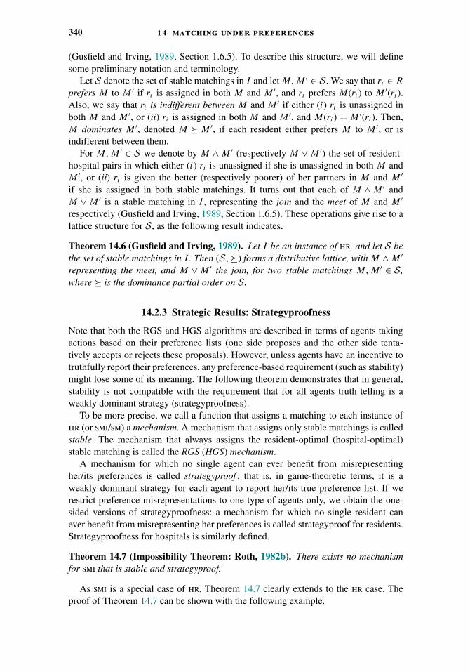
340 1 4 matching under preferences
(Gusfield and Irving, 1989, Section 1.6.5). To describe this structure, we will definesome preliminary notation and terminology.
Let S denote the set of stable matchings in I and let M, M ′ ∈ S . We say that ri ∈ R
prefers M to M ′ if ri is assigned in both M and M ′, and ri prefers M(ri) to M ′(ri).Also, we say that ri is indifferent between M and M ′ if either (i) ri is unassigned inboth M and M ′, or (ii) ri is assigned in both M and M ′, and M(ri) = M ′(ri). Then,M dominates M ′, denoted M - M ′, if each resident either prefers M to M ′, or isindifferent between them.
For M, M ′ ∈ S we denote by M ∧ M ′ (respectively M ∨ M ′) the set of resident-hospital pairs in which either (i) ri is unassigned if she is unassigned in both M andM ′, or (ii) ri is given the better (respectively poorer) of her partners in M and M ′
if she is assigned in both stable matchings. It turns out that each of M ∧ M ′ andM ∨ M ′ is a stable matching in I , representing the join and the meet of M and M ′
respectively (Gusfield and Irving, 1989, Section 1.6.5). These operations give rise to alattice structure for S , as the following result indicates.
Theorem 14.6 (Gusfield and Irving, 1989). Let I be an instance of hr, and let S bethe set of stable matchings in I . Then (S,-) forms a distributive lattice, with M ∧ M ′
representing the meet, and M ∨ M ′ the join, for two stable matchings M, M ′ ∈ S ,where - is the dominance partial order on S .
14.2.3 Strategic Results: Strategyproofness
Note that both the RGS and HGS algorithms are described in terms of agents takingactions based on their preference lists (one side proposes and the other side tenta-tively accepts or rejects these proposals). However, unless agents have an incentive totruthfully report their preferences, any preference-based requirement (such as stability)might lose some of its meaning. The following theorem demonstrates that in general,stability is not compatible with the requirement that for all agents truth telling is aweakly dominant strategy (strategyproofness).
To be more precise, we call a function that assigns a matching to each instance ofhr (or smi/sm) a mechanism. A mechanism that assigns only stable matchings is calledstable. The mechanism that always assigns the resident-optimal (hospital-optimal)stable matching is called the RGS (HGS) mechanism.
A mechanism for which no single agent can ever benefit from misrepresentingher/its preferences is called strategyproof , that is, in game-theoretic terms, it is aweakly dominant strategy for each agent to report her/its true preference list. If werestrict preference misrepresentations to one type of agents only, we obtain the one-sided versions of strategyproofness: a mechanism for which no single resident canever benefit from misrepresenting her preferences is called strategyproof for residents.Strategyproofness for hospitals is similarly defined.
Theorem 14.7 (Impossibility Theorem: Roth, 1982b). There exists no mechanismfor smi that is stable and strategyproof.
As smi is a special case of hr, Theorem 14.7 clearly extends to the hr case. Theproof of Theorem 14.7 can be shown with the following example.

1 4 .2 two-sided preferences 341
Example 14.8 (Impossibility). Consider the following instance:
r1 : h1 h2 h1 : r2 r1
r2 : h2 h1 h2 : r1 r2
The two stable matchings for this instance are Ma = {(r1, h1), (r2, h2)} and Mz ={(r1, h2), (r2, h1)}. Assume that the mechanism picks stable matching Ma . Then, if h1
pretended that only r2 is acceptable, Ma is not stable anymore and the stable mechanismwould have to pick the only remaining stable matching Mz, which h1 would prefer; acontradiction to strategyproofness. Similarly, if the mechanism picks stable matchingMz, r1 could manipulate by declaring h1 uniquely acceptable.
The intuition behind this impossibility result is that an agent who is assigned toa stable partner that is not her/its best stable partner can improve her/its outcomeby truncating the preference list just below the best stable partner: this unilateralmanipulation will result in the assignment of the best stable partner to the agentwho misrepresented her/its preference list. Alcalde and Barbera (1994) and Takagiand Serizawa (2010) further strengthened the impossibility result by considerablyweakening the stability requirement.
On the positive side, stable mechanisms that respect strategyproofness for all resi-dents exist.
Theorem 14.9 (Roth, 1985). The RGS mechanism for hr is strategyproof for residents.
As hr is a generalization of each of sm and smi, clearly Theorem 14.9 also holdsin these latter contexts. This theorem for hr is an extension of an earlier correspond-ing theorem for sm (Dubins and Freedman, 1981; Roth, 1982a). Strategyproofness forall residents also turns out to be a key property in characterizing the RGS mechanism(Ehlers and Klaus, 2014): almost all real-life mechanisms used in variants of hr (includ-ing sc)—including the large classes of priority mechanisms and linear programmingmechanisms—satisfy a set of simple and intuitive properties, but once strategyproof-ness is added to these properties, the RGS mechanism is the only one surviving (andcharacterized by the respective properties including strategyproofness). For sc, sinceresidents (aka students) are the only economic agents, Theorem 14.9 in fact estab-lishes a possibility result. For hr, the negative result of Theorem 14.7 persists even ifrestricting attention only to hospitals.
Theorem 14.10 (Roth, 1986). There exists no mechanism for hr that is stable andstrategyproof for hospitals.
This result implies that even when the HGS mechanism is used, hospitals mighthave an incentive to misrepresent their preferences.
Once the incompatibility of stability and strategyproofness is established(Theorems 14.7 and 14.10), the question arises as to whether we can at least findstable mechanisms that are resistant to strategic behavior, meaning that it is compu-tationally difficult (i.e., NP-hard) for agents to behave strategically. This approach istypical in voting theory, which is the subject of Chapter 6 on barriers to manipulation,because no voting rule is strategyproof (Arrow et al., 2002; Bartholdi et al., 1989a).It is possible to exploit such results to define stable mechanisms that are resistant to
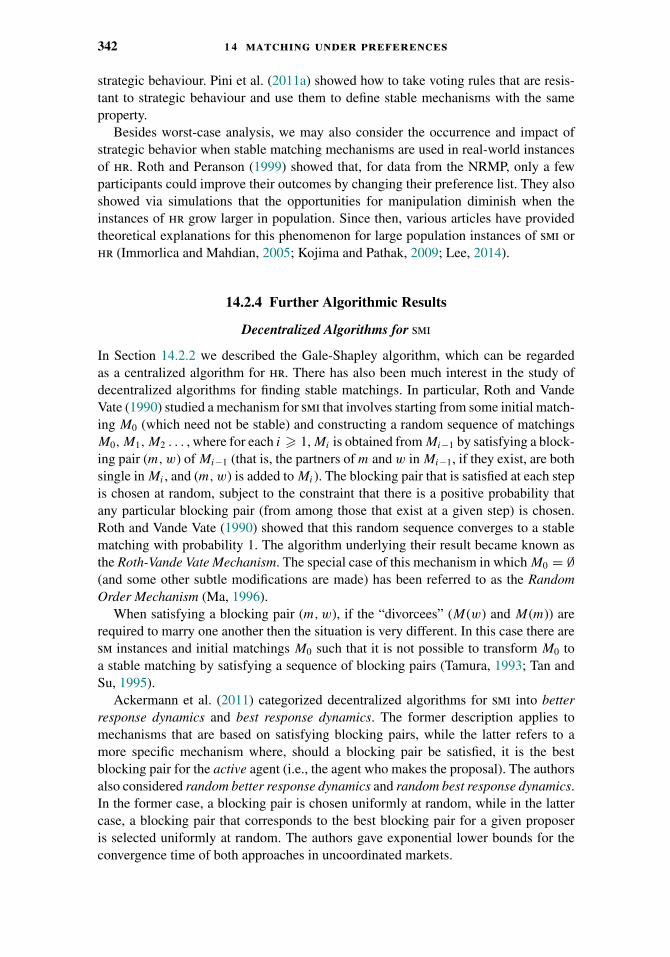
342 1 4 matching under preferences
strategic behaviour. Pini et al. (2011a) showed how to take voting rules that are resis-tant to strategic behaviour and use them to define stable mechanisms with the sameproperty.
Besides worst-case analysis, we may also consider the occurrence and impact ofstrategic behavior when stable matching mechanisms are used in real-world instancesof hr. Roth and Peranson (1999) showed that, for data from the NRMP, only a fewparticipants could improve their outcomes by changing their preference list. They alsoshowed via simulations that the opportunities for manipulation diminish when theinstances of hr grow larger in population. Since then, various articles have providedtheoretical explanations for this phenomenon for large population instances of smi orhr (Immorlica and Mahdian, 2005; Kojima and Pathak, 2009; Lee, 2014).
14.2.4 Further Algorithmic Results
Decentralized Algorithms for smi
In Section 14.2.2 we described the Gale-Shapley algorithm, which can be regardedas a centralized algorithm for hr. There has also been much interest in the study ofdecentralized algorithms for finding stable matchings. In particular, Roth and VandeVate (1990) studied a mechanism for smi that involves starting from some initial match-ing M0 (which need not be stable) and constructing a random sequence of matchingsM0, M1, M2 . . . , where for each i � 1, Mi is obtained from Mi−1 by satisfying a block-ing pair (m, w) of Mi−1 (that is, the partners of m and w in Mi−1, if they exist, are bothsingle in Mi , and (m, w) is added to Mi). The blocking pair that is satisfied at each stepis chosen at random, subject to the constraint that there is a positive probability thatany particular blocking pair (from among those that exist at a given step) is chosen.Roth and Vande Vate (1990) showed that this random sequence converges to a stablematching with probability 1. The algorithm underlying their result became known asthe Roth-Vande Vate Mechanism. The special case of this mechanism in which M0 = ∅(and some other subtle modifications are made) has been referred to as the RandomOrder Mechanism (Ma, 1996).
When satisfying a blocking pair (m, w), if the “divorcees” (M(w) and M(m)) arerequired to marry one another then the situation is very different. In this case there aresm instances and initial matchings M0 such that it is not possible to transform M0 toa stable matching by satisfying a sequence of blocking pairs (Tamura, 1993; Tan andSu, 1995).
Ackermann et al. (2011) categorized decentralized algorithms for smi into betterresponse dynamics and best response dynamics. The former description applies tomechanisms that are based on satisfying blocking pairs, while the latter refers to amore specific mechanism where, should a blocking pair be satisfied, it is the bestblocking pair for the active agent (i.e., the agent who makes the proposal). The authorsalso considered random better response dynamics and random best response dynamics.In the former case, a blocking pair is chosen uniformly at random, while in the lattercase, a blocking pair that corresponds to the best blocking pair for a given proposeris selected uniformly at random. The authors gave exponential lower bounds for theconvergence time of both approaches in uncoordinated markets.
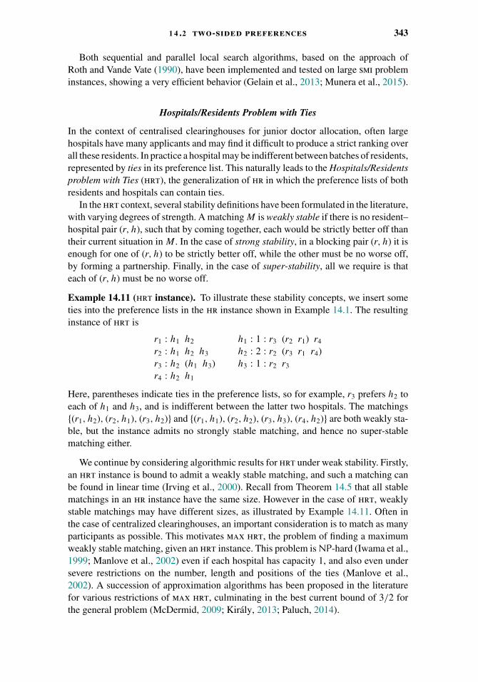
1 4 .2 two-sided preferences 343
Both sequential and parallel local search algorithms, based on the approach ofRoth and Vande Vate (1990), have been implemented and tested on large smi probleminstances, showing a very efficient behavior (Gelain et al., 2013; Munera et al., 2015).
Hospitals/Residents Problem with Ties
In the context of centralised clearinghouses for junior doctor allocation, often largehospitals have many applicants and may find it difficult to produce a strict ranking overall these residents. In practice a hospital may be indifferent between batches of residents,represented by ties in its preference list. This naturally leads to the Hospitals/Residentsproblem with Ties (hrt), the generalization of hr in which the preference lists of bothresidents and hospitals can contain ties.
In the hrt context, several stability definitions have been formulated in the literature,with varying degrees of strength. A matching M is weakly stable if there is no resident–hospital pair (r, h), such that by coming together, each would be strictly better off thantheir current situation in M . In the case of strong stability, in a blocking pair (r, h) it isenough for one of (r, h) to be strictly better off, while the other must be no worse off,by forming a partnership. Finally, in the case of super-stability, all we require is thateach of (r, h) must be no worse off.
Example 14.11 (hrt instance). To illustrate these stability concepts, we insert someties into the preference lists in the hr instance shown in Example 14.1. The resultinginstance of hrt is
r1 : h1 h2 h1 : 1 : r3 (r2 r1) r4
r2 : h1 h2 h3 h2 : 2 : r2 (r3 r1 r4)r3 : h2 (h1 h3) h3 : 1 : r2 r3
r4 : h2 h1
Here, parentheses indicate ties in the preference lists, so for example, r3 prefers h2 toeach of h1 and h3, and is indifferent between the latter two hospitals. The matchings{(r1, h2), (r2, h1), (r3, h2)} and {(r1, h1), (r2, h2), (r3, h3), (r4, h2)} are both weakly sta-ble, but the instance admits no strongly stable matching, and hence no super-stablematching either.
We continue by considering algorithmic results for hrt under weak stability. Firstly,an hrt instance is bound to admit a weakly stable matching, and such a matching canbe found in linear time (Irving et al., 2000). Recall from Theorem 14.5 that all stablematchings in an hr instance have the same size. However in the case of hrt, weaklystable matchings may have different sizes, as illustrated by Example 14.11. Often inthe case of centralized clearinghouses, an important consideration is to match as manyparticipants as possible. This motivates max hrt, the problem of finding a maximumweakly stable matching, given an hrt instance. This problem is NP-hard (Iwama et al.,1999; Manlove et al., 2002) even if each hospital has capacity 1, and also even undersevere restrictions on the number, length and positions of the ties (Manlove et al.,2002). A succession of approximation algorithms has been proposed in the literaturefor various restrictions of max hrt, culminating in the best current bound of 3/2 forthe general problem (McDermid, 2009; Kiraly, 2013; Paluch, 2014).

344 1 4 matching under preferences
Although an hrt instance I is bound to admit a weakly stable matching as mentionedabove, by contrast a strongly stable matching or a super-stable matching in I may notexist (Irving et al., 2000, 2003). However there is an efficient algorithm to find astrongly stable matching or report that none exists (Kavitha et al., 2007). A faster andsimpler algorithm exists in the case of super-stability (Irving et al., 2000). Moreoveran analogue of Theorem 14.5 holds in hrt under each of the strong stability andsuper-stability criteria (Scott, 2005; Irving et al., 2000).
Hospitals/Residents Problem with Couples
Another variant of hr that is motivated by practical applications arises in the presenceof couples. These are pairs of residents who wish to be jointly assigned to hospitals via acommon preferences list over pairs of hospitals, typically in order to be geographicallyclose to one another. Each couple (ri, rj ) has a preference list over a subset of H × H ,where each pair (hp, hq) on this list represents the joint assignment of ri to hp andrj to hq . (There may be single residents in addition, as before.) We thus obtain theHospitals/Residents problem with Couples (hrc).
Relative to a suitable stability definition, Roth (1984a) showed that an hrc instanceneed not admit a stable matching. Ng and Hirschberg (1988) and Ronn (1990) indepen-dently showed that the problem of deciding whether an hrc instance admits a stablematching is NP-complete, even if each hospital has capacity 1 and there are no singleresidents.
McDermid and Manlove (2010) considered a variant of hrc in which each resident(whether single or in a couple) has a preference list over individual hospitals, and thejoint preference list of each couple (ri, rj ) is consistent with the individual lists of ri andrj in a precise sense. Relative to Roth’s stability definition (Roth, 1984a), they showedthat the problem of deciding whether a stable matching exists is NP-complete. Howeverif instead we enforce classical (Gale–Shapley) stability on a given matching relative tothe individual lists of residents, then the problem of finding a stable matching or report-ing that none exists is solvable in polynomial time (McDermid and Manlove, 2010).
Biro et al. (2011) developed a range of heuristics for the problem of finding a stablematching or reporting that none exists in a given hrc instance, and subjected them toa detailed empirical evaluation based on randomly generated data. They found that astable matching is very likely to exist for instances where the ratio of couples to singleresidents is small and of the magnitude typically found in practical applications.
Ashlagi et al. (2014) studied large random matching markets with couples. Theyintroduced a new matching algorithm and showed that if the number of couples growsslower than the size of the market, a stable matching will be found with high probability.If, however, the number of couples grows at a linear rate, with constant probability (notdepending on the market size), no stable matching exists.
Further results for hrc are described in the survey paper of Biro and Klijn (2013).
Many-to-Many Stable Matching
Many-to-many extensions of sm (and by implication hr) have been considered inthe literature (Roth, 1984b; Roth and Sotomayor, 1990; Sotomayor, 1999; Baıou and

1 4 .3 one-sided preferences 345
Balinski, 2000; Fleiner, 2003; Martınez et al., 2004; Echenique and Oviedo, 2006;Bansal et al., 2007; Kojima and Unver, 2008; Eirinakis et al., 2012, 2013; Klijn andYazıcı, 2014). These matching problems tend to be described in the context of assigningworkers to firms, where each agent can be multiply assigned (up to a given capacity).We will discuss the two main models of many-to-many matching in the literature.
The first version we consider, which we refer to as the Workers/Firms problem,Version 1, denoted by wf-1, involves each worker ranking in strict order of preferencea set of individual acceptable firms, and vice versa for each firm. Baıou and Balinski(2000) generalized the stability definition for sm to the wf-1 case. They showed thatevery instance I of wf-1 has a stable matching and such a matching can be found inO(n2) time, where n = max{n1, n2}, n1 is the number of workers and n2 is the numberof firms in I . They also generalized Theorems 14.5 and 14.6 to the wf-1 context.Additional algorithms have been given for computing stable matchings with variousoptimality properties in wf-1 (Bansal et al., 2007; Eirinakis et al., 2012, 2013).
In the second version, which we refer to as the Workers/Firms problem, Version 2,denoted by wf-2, each worker ranks in strict order of preference acceptable subsets offirms, and vice versa for each firm. Two main forms of stability have been studied inthe context of wf-2, namely, pairwise stability and setwise stability.
A matching M in a wf-2 instance is pairwise stable (Roth, 1984b) if it cannot beundermined by a single worker–firm pair acting together. A wf-2 instance need notadmit a pairwise stable matching (Roth and Sotomayor, 1990, Example 2.7). HoweverRoth (1984b) proved that, given an instance of wf-2 where every agent’s preferencelist satisfies so-called substitutability (Kelso and Crawford, 1982), a pairwise stablematching always exists, and he gave an algorithm for finding one. Martınez et al. (2004)gave an algorithm for finding all pairwise stable matchings.
A more powerful definition of stability is setwise stability. Informally, a matching M
is setwise stable (Sotomayor, 1999) if it cannot be undermined by a coalition of workersand firms acting together. More precisely, several definitions of setwise stability havebeen given in the literature (Sotomayor, 1999; Echenique and Oviedo, 2006; Konishiand Unver, 2006); the various alternatives were formally defined and analyzed by Klausand Walzl (2009).
Bansal et al. (2007) noted that, generally speaking, wf-1 has been studied mainly bythe computer science community, while the economics community has mainly focusedon wf-2. One reason for this is that wf-2 suffers from the drawback that the length ofan agent’s preference list is in the worst case exponential in the number of agents. Aconsequence of this is that the practical applicability of any algorithm for wf-2 wouldbe severely limited in general, however, this problem does not arise with wf-1.
14.3 One-Sided Preferences
14.3.1 Introduction and Preliminary Definitions
Many economists and game theorists, and increasingly computer scientists in recentyears, have studied the problem of allocating a set H of indivisible goods among aset A of applicants (Shapley and Scarf, 1974; Hylland and Zeckhauser, 1979; Deng
346 1 4 matching under preferences
et al., 2003; Fekete et al., 2003). Each applicant ai may have ordinal preferences over asubset of H (the acceptable goods for ai). Many models have considered the case wherethere is no monetary transfer. In the literature the situation in which each applicantinitially owns one good is known as a Housing Market (hm)3 (Shapley and Scarf,1974; Roth and Postlewaite, 1977; Roth, 1982b). When there are no initial propertyrights, we obtain the House Allocation problem (ha) (Hylland and Zeckhauser, 1979;Zhou, 1990; Abdulkadiroglu and Sonmez, 1998). A mixed model, in which a subset ofapplicants initially owns a good has also been studied (Abdulkadiroglu and Sonmez,1999).
House Allocation Problems
Formally, an instance I of the House Allocation problem (ha) comprises a set A ={a1, a2, . . . , an1} of applicants and a set H = {h1, h2, . . . , hn2} of houses. The agentsin I are the applicants and houses in A ∪ H . There is a set E ⊆ A × H of acceptableapplicant–house pairs. Let m = |E|. Each applicant ai ∈ A has an acceptable set ofhouses A(ai), where A(ai) = {hj ∈ H : (ai, hj ) ∈ E}. Similarly each house hj ∈ H
has an acceptable set of applicants A(hj ), where A(hj ) = {ai ∈ A : (ai, hj ) ∈ E}.Each applicant ai ∈ A has a preference list in which she ranks A(ai) in strict order.
Given any applicant ai ∈ A, and given any houses hj , hk ∈ H , ai is said to prefer hj tohk if {hj , hk} ⊆ A(ai), and hj precedes hk on ai’s preference list. Houses do not havepreference lists over applicants, and it is essentially this feature that distinguishes hafrom smi.
ha is a very general problem model and any application domain having an underlyingmatching problem that is bipartite, where agents in only one of the sets have preferencesover the other, can be viewed as an instance of ha. These include the problems ofallocating graduates to trainee positions, students to projects, professors to offices,clients to servers, and so on. The literature concerning ha has largely described thisproblem model in terms of assigning applicants to houses, so for consistency we alsoadopt this terminology.
An assignment M in I is a subset of E. The definitions of the terms assigned to,assigned, unassigned and assignees relative to M are analogous to the same definitionsin the hr case (see Section 14.2.1). A matching M in I is an assignment such that,for each pk ∈ A ∪ H , the set of assignees of pk in M , denoted by M(pk), satisfies|M(pk)| � 1. For notational convenience, as in the hr case, if pk is assigned in M
then where there is no ambiguity the notation M(pk) is also used to refer to the singlemember of the set M(pk). Let M denote the set of matchings in I .
Given two matchings M and M ′ in M, we say that an applicant ai ∈ A prefers M ′
to M if either (i) ai is assigned in M ′ and unassigned in M , or (ii) ai is assigned inboth M and M ′, and ai prefers M ′(ai) to M(ai). We say that M ′ Pareto dominates M if(i) some applicant prefers M ′ to M and (ii) no applicant prefers M to M ′. A matchingM ∈ M is Pareto optimal if there is no matching M ′ ∈ M that Pareto dominates M .Intuitively M is Pareto optimal if no applicant ai can be better off without requiring
3 This problem is also referred to as the House-swapping Game in the literature.
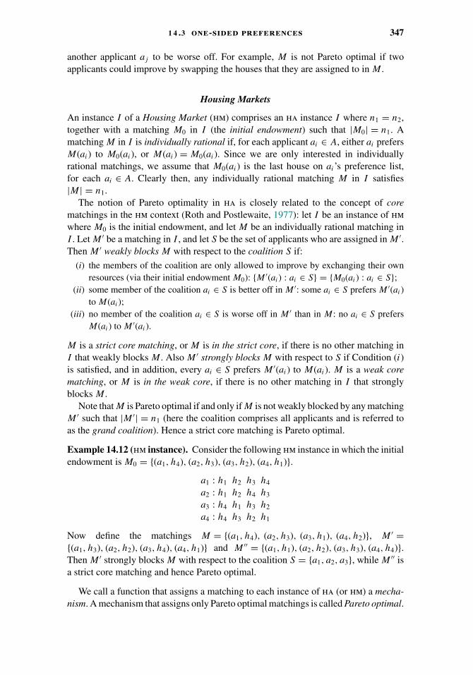
1 4 .3 one-sided preferences 347
another applicant aj to be worse off. For example, M is not Pareto optimal if twoapplicants could improve by swapping the houses that they are assigned to in M .
Housing Markets
An instance I of a Housing Market (hm) comprises an ha instance I where n1 = n2,together with a matching M0 in I (the initial endowment) such that |M0| = n1. Amatching M in I is individually rational if, for each applicant ai ∈ A, either ai prefersM(ai) to M0(ai), or M(ai) = M0(ai). Since we are only interested in individuallyrational matchings, we assume that M0(ai) is the last house on ai’s preference list,for each ai ∈ A. Clearly then, any individually rational matching M in I satisfies|M| = n1.
The notion of Pareto optimality in ha is closely related to the concept of corematchings in the hm context (Roth and Postlewaite, 1977): let I be an instance of hmwhere M0 is the initial endowment, and let M be an individually rational matching inI . Let M ′ be a matching in I , and let S be the set of applicants who are assigned in M ′.Then M ′ weakly blocks M with respect to the coalition S if:
(i) the members of the coalition are only allowed to improve by exchanging their ownresources (via their initial endowment M0): {M ′(ai) : ai ∈ S} = {M0(ai) : ai ∈ S};
(ii) some member of the coalition ai ∈ S is better off in M ′: some ai ∈ S prefers M ′(ai)to M(ai);
(iii) no member of the coalition ai ∈ S is worse off in M ′ than in M: no ai ∈ S prefersM(ai) to M ′(ai).
M is a strict core matching, or M is in the strict core, if there is no other matching inI that weakly blocks M . Also M ′ strongly blocks M with respect to S if Condition (i)is satisfied, and in addition, every ai ∈ S prefers M ′(ai) to M(ai). M is a weak corematching, or M is in the weak core, if there is no other matching in I that stronglyblocks M .
Note that M is Pareto optimal if and only if M is not weakly blocked by any matchingM ′ such that |M ′| = n1 (here the coalition comprises all applicants and is referred toas the grand coalition). Hence a strict core matching is Pareto optimal.
Example 14.12 (hm instance). Consider the following hm instance in which the initialendowment is M0 = {(a1, h4), (a2, h3), (a3, h2), (a4, h1)}.
a1 : h1 h2 h3 h4
a2 : h1 h2 h4 h3
a3 : h4 h1 h3 h2
a4 : h4 h3 h2 h1
Now define the matchings M = {(a1, h4), (a2, h3), (a3, h1), (a4, h2)}, M ′ ={(a1, h3), (a2, h2), (a3, h4), (a4, h1)} and M ′′ = {(a1, h1), (a2, h2), (a3, h3), (a4, h4)}.Then M ′ strongly blocks M with respect to the coalition S = {a1, a2, a3}, while M ′′ isa strict core matching and hence Pareto optimal.
We call a function that assigns a matching to each instance of ha (or hm) a mecha-nism. A mechanism that assigns only Pareto optimal matchings is called Pareto optimal.
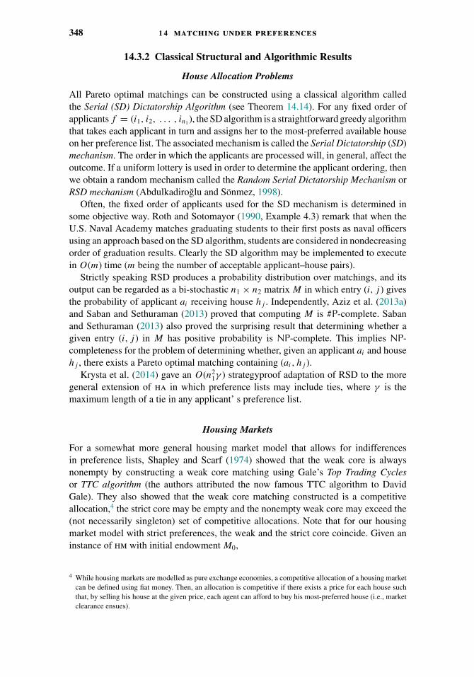
348 1 4 matching under preferences
14.3.2 Classical Structural and Algorithmic Results
House Allocation Problems
All Pareto optimal matchings can be constructed using a classical algorithm calledthe Serial (SD) Dictatorship Algorithm (see Theorem 14.14). For any fixed order ofapplicants f = (i1, i2, . . . , in1 ), the SD algorithm is a straightforward greedy algorithmthat takes each applicant in turn and assigns her to the most-preferred available houseon her preference list. The associated mechanism is called the Serial Dictatorship (SD)mechanism. The order in which the applicants are processed will, in general, affect theoutcome. If a uniform lottery is used in order to determine the applicant ordering, thenwe obtain a random mechanism called the Random Serial Dictatorship Mechanism orRSD mechanism (Abdulkadiroglu and Sonmez, 1998).
Often, the fixed order of applicants used for the SD mechanism is determined insome objective way. Roth and Sotomayor (1990, Example 4.3) remark that when theU.S. Naval Academy matches graduating students to their first posts as naval officersusing an approach based on the SD algorithm, students are considered in nondecreasingorder of graduation results. Clearly the SD algorithm may be implemented to executein O(m) time (m being the number of acceptable applicant–house pairs).
Strictly speaking RSD produces a probability distribution over matchings, and itsoutput can be regarded as a bi-stochastic n1 × n2 matrix M in which entry (i, j ) givesthe probability of applicant ai receiving house hj . Independently, Aziz et al. (2013a)and Saban and Sethuraman (2013) proved that computing M is #P-complete. Sabanand Sethuraman (2013) also proved the surprising result that determining whether agiven entry (i, j ) in M has positive probability is NP-complete. This implies NP-completeness for the problem of determining whether, given an applicant ai and househj , there exists a Pareto optimal matching containing (ai, hj ).
Krysta et al. (2014) gave an O(n21γ ) strategyproof adaptation of RSD to the more
general extension of ha in which preference lists may include ties, where γ is themaximum length of a tie in any applicant’ s preference list.
Housing Markets
For a somewhat more general housing market model that allows for indifferencesin preference lists, Shapley and Scarf (1974) showed that the weak core is alwaysnonempty by constructing a weak core matching using Gale’s Top Trading Cyclesor TTC algorithm (the authors attributed the now famous TTC algorithm to DavidGale). They also showed that the weak core matching constructed is a competitiveallocation,4 the strict core may be empty and the nonempty weak core may exceed the(not necessarily singleton) set of competitive allocations. Note that for our housingmarket model with strict preferences, the weak and the strict core coincide. Given aninstance of hm with initial endowment M0,
4 While housing markets are modelled as pure exchange economies, a competitive allocation of a housing marketcan be defined using fiat money. Then, an allocation is competitive if there exists a price for each house suchthat, by selling his house at the given price, each agent can afford to buy his most-preferred house (i.e., marketclearance ensues).
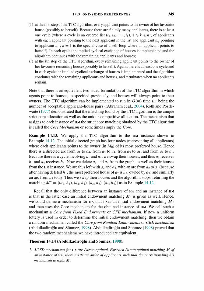
1 4 .3 one-sided preferences 349
(1) at the first step of the TTC algorithm, every applicant points to the owner of her favouritehouse (possibly to herself). Because there are finitely many applicants, there is at leastone cycle (where a cycle is an ordered list (i1, i2, . . . , ik), 1 � k � n1, of applicantswith each applicant pointing to the next applicant in the list and applicant aik pointingto applicant ai1 ; k = 1 is the special case of a self-loop where an applicant points toherself). In each cycle the implied cyclical exchange of houses is implemented and thealgorithm continues with the remaining applicants and houses;
(l) at the lth step of the TTC algorithm, every remaining applicant points to the owner ofher favourite remaining house (possibly to herself). Again, there is at least one cycle andin each cycle the implied cyclical exchange of houses is implemented and the algorithmcontinues with the remaining applicants and houses, and terminates when no applicantsremain.
Note that there is an equivalent two-sided formulation of the TTC algorithm in whichagents point to houses, as specified previously, and houses will always point to theirowners. The TTC algorithm can be implemented to run in O(m) time (m being thenumber of acceptable applicant–house pairs) (Abraham et al., 2004). Roth and Postle-waite (1977) demonstrated that the matching found by the TTC algorithm is the uniquestrict core allocation as well as the unique competitive allocation. The mechanism thatassigns to each instance of hm the strict core matching obtained by the TTC algorithmis called the Core Mechanism or sometimes simply the Core.
Example 14.13. We apply the TTC algorithm to the hm instance shown inExample 14.12. The initial directed graph has four nodes (representing all applicants)where each applicants points to the owner (in M0) of its most preferred house. Hencethere is a directed arc from a1 to a4, from a2 to a4, from a3 to a1, and from a4 to a1.Because there is a cycle involving a1 and a4, we swap their houses, and thus a1 receivesh1 and a4 receives h4. Now we delete a1 and a4 from the graph, as well as their housesfrom the hm instance. We are thus left with a2 and a3, with an arc from a2 to a3 (becauseafter having deleted h1, the most preferred house of a2 is h2, owned by a3) and similarlyan arc from a3 to a2. Thus we swap their houses and the algorithm stops, returning thematching M ′′ = {(a1, h1), (a2, h2), (a3, h3), (a4, h4)} as in Example 14.12.
Recall that the only difference between an instance of ha and an instance of hmis that in the latter case an initial endowment matching M0 is given as well. Hence,we could define a mechanism for ha that fixes an initial endowment matching Mf
and then uses the Core mechanism for the obtained instance of hm. We call such amechanism a Core from Fixed Endowments or CFE mechanism. If now a uniformlottery is used in order to determine the initial endowment matching, then we obtaina random mechanism called the Core from Random Endowments or CRE mechanism(Abdulkadiroglu and Sonmez, 1998). Abdulkadiroglu and Sonmez (1998) proved thatthe two random mechanisms we have introduced are equivalent.
Theorem 14.14 (Abdulkadiroglu and Sonmez, 1998).
1. All SD mechanisms for ha are Pareto optimal. For each Pareto optimal matching M ofan instance of ha, there exists an order of applicants such that the corresponding SDmechanism assigns M .

350 1 4 matching under preferences
2. All Core mechanisms for hm are Pareto optimal. For each Pareto optimal matching M
of an instance of ha, there exists an initial endowment matching Mf such that the CFEmechanism assigns M .
3. The CRE and the RSD mechanisms for ha are equivalent.
Hylland and Zeckhauser (1979) had already shown that the RSD mechanism isex-post Pareto optimal, that is, the final matching that is chosen by the RSD lotteryis Pareto optimal. Bogomolnaia and Moulin (2001) showed that the RSD mechanism,however, is not ex ante or ordinally efficient (Pareto optimal), that is, for some lotterieschosen by the RSD mechanism there exist Pareto dominating lotteries (with stochasticdominance being used to formulate the dominance relation). They also suggested anew random mechanism, the Probabilistic Serial mechanism, that satisfies ex anteefficiency.
14.3.3 Strategic Results: Strategyproofness
As in Section 14.2.1, a mechanism for which no single applicant can ever benefit frommisrepresenting her preferences is called strategyproof (i.e., in game-theoretic terms,it is a weakly dominant strategy for each applicant to report her true preference list).All mechanisms introduced so far in this section are strategyproof, as the followingresults indicate.
Theorem 14.15 (Hylland and Zeckhauser, 1979). The SD mechanisms for ha arestrategyproof.
Theorem 14.16 (Roth, 1982b). The Core mechanism for hm is strategyproof. Hence,all CFE mechanisms for ha are strategyproof.
In addition, the Core and CFE mechanisms are group strategyproof (i.e., no coalitionof applicants can jointly misrepresent their true preferences in order for at least onemember of the coalition to improve, while no other coalition member is worse off; see,e.g., Svensson, 1999). Strategyproofness is also one of the properties that characterizethe Core mechanism.
Theorem 14.17 (Ma, 1994). The Core mechanism for hm is the only mechanism thatis Pareto optimal, individually rational, and strategyproof.
Abdulkadiroglu and Sonmez (1999) extended Ma’s characterization result to a mixedmodel that combines ha and hm: in the House Allocation problem with ExistingTenants, a subset of applicants initially owns a house. They defined mechanismsthat combine elements of SD as well as Core mechanisms based on the so-calledYRMH-IGYT (You Request My House—I Get Your Turn) algorithm. All YRMH-IGYT mechanisms are strategyproof, Pareto optimal, and individually rational (in thesense that no existing tenant receives a house inferior to his own).
In Section 14.2.1 we introduced sc as a one-sided preference variant of hr, butwe could also introduce this class of problems as a variant of ha with the additionalproperties that objects (i.e., houses/schools) have priorities over students, and objectscan be multiply assigned up to some capacity. Either way, the RGS mechanism can beused to find a matching for each instance of sc. This mechanism is then strategyproof
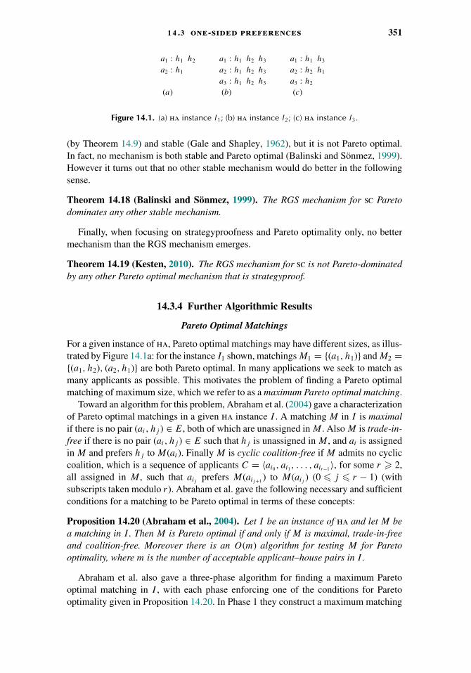
1 4 .3 one-sided preferences 351
a1 : h1 h2 a1 : h1 h2 h3 a1 : h1 h3
a2 : h1 a2 : h1 h2 h3 a2 : h2 h1
a3 : h1 h2 h3 a3 : h2
(a) (b) (c)
Figure 14.1. (a) ha instance I1; (b) ha instance I2; (c) ha instance I3.
(by Theorem 14.9) and stable (Gale and Shapley, 1962), but it is not Pareto optimal.In fact, no mechanism is both stable and Pareto optimal (Balinski and Sonmez, 1999).However it turns out that no other stable mechanism would do better in the followingsense.
Theorem 14.18 (Balinski and Sonmez, 1999). The RGS mechanism for sc Paretodominates any other stable mechanism.
Finally, when focusing on strategyproofness and Pareto optimality only, no bettermechanism than the RGS mechanism emerges.
Theorem 14.19 (Kesten, 2010). The RGS mechanism for sc is not Pareto-dominatedby any other Pareto optimal mechanism that is strategyproof.
14.3.4 Further Algorithmic Results
Pareto Optimal Matchings
For a given instance of ha, Pareto optimal matchings may have different sizes, as illus-trated by Figure 14.1a: for the instance I1 shown, matchings M1 = {(a1, h1)} and M2 ={(a1, h2), (a2, h1)} are both Pareto optimal. In many applications we seek to match asmany applicants as possible. This motivates the problem of finding a Pareto optimalmatching of maximum size, which we refer to as a maximum Pareto optimal matching.
Toward an algorithm for this problem, Abraham et al. (2004) gave a characterizationof Pareto optimal matchings in a given ha instance I . A matching M in I is maximalif there is no pair (ai, hj ) ∈ E, both of which are unassigned in M . Also M is trade-in-free if there is no pair (ai, hj ) ∈ E such that hj is unassigned in M , and ai is assignedin M and prefers hj to M(ai). Finally M is cyclic coalition-free if M admits no cycliccoalition, which is a sequence of applicants C = 〈ai0, ai1, . . . , air−1〉, for some r � 2,all assigned in M , such that aij prefers M(aij+1 ) to M(aij ) (0 � j � r − 1) (withsubscripts taken modulo r). Abraham et al. gave the following necessary and sufficientconditions for a matching to be Pareto optimal in terms of these concepts:
Proposition 14.20 (Abraham et al., 2004). Let I be an instance of ha and let M bea matching in I . Then M is Pareto optimal if and only if M is maximal, trade-in-freeand coalition-free. Moreover there is an O(m) algorithm for testing M for Paretooptimality, where m is the number of acceptable applicant–house pairs in I .
Abraham et al. also gave a three-phase algorithm for finding a maximum Paretooptimal matching in I , with each phase enforcing one of the conditions for Paretooptimality given in Proposition 14.20. In Phase 1 they construct a maximum matching
352 1 4 matching under preferences
M in the underlying graph of I , which is the bipartite graph with vertex set A ∪ H
and edge set E. This step can be accomplished in O(√
n1m) time and ensures thatM is maximal. Phase 2 is based on an O(m) algorithm in which assigned applicantsrepeatedly trade in their own house in M for any preferred vacant house. Once this stepterminates, M is trade-in-free. Finally, cyclic coalitions are eliminated during Phase 3,which is based on an O(m) implementation of the TTC algorithm. Putting these threephases together, they obtained the following result.
Theorem 14.21 (Abraham et al., 2004). Let I be an instance of ha. A maximumPareto optimal matching in I can be found in O(
√n1m) time, where n1 is the number
of applicants and m is the number of acceptable applicant–house pairs in I .
Popular Matchings
Pareto optimality is a fundamental solution concept, but on its own it is a relativelyweak property. A stronger notion is that of a popular matching. Intuitively a matchingM in an ha instance I is popular if there is no other matching that is preferred to M bya majority of the applicants who are not indifferent between the two matchings. Thisconcept was first defined by Gardenfors (1975) (using the term majority assignment)in the context of smi.
To define the popular matching concept more formally, let M, M ′ ∈ M, and letP (M, M ′) denote the set of applicants who prefer M to M ′. We say that M ′ is morepopular than M , denoted M ′ � M , if |P (M ′, M)| > |P (M, M ′)|. Define a matchingM ∈ M to be popular (Abraham et al., 2007b) if M is �-maximal (i.e., there is noother matching M ′ ∈ M such that M ′ � M).
Clearly a matching M is Pareto optimal if there is no other matching M ′ suchthat |P (M, M ′)| = 0 and |P (M ′, M)| � 1. Hence a popular matching is Pareto opti-mal. However in contrast to the case for Pareto optimal matchings, an ha instanceneed not admit a popular matching. To see this, consider the ha instance I2 shownin Figure 14.1b. It is clear that a matching in I2 cannot be popular unless all appli-cants are assigned. The unique matching up to symmetry in which all applicants areassigned is M = {(ai, hi) : 1 � i � 3}, however, M ′ = {(a2, h1), (a3, h2)} is preferredby two applicants, which is a majority. The relation � in this case cycles, hencethe absence of a �-maximal solution (therefore, in general, � is not a partial orderon M).
The potential absence of a popular matching in a given ha instance can berelated all the way back to the observation of Condorcet (1785) that, given k vot-ers who each rank n candidates in strict order of preference, there may not exist a“winner,” namely, a candidate who beats all others in a pairwise majority vote. See alsoChapter 2.
Abraham et al. (2007b) derived a neat characterization of popular matchings, leadingto an O(m) algorithm to check whether a given matching M in I is popular. The samecharacterization also led naturally to an O(n + m) algorithm for finding a popularmatching or reporting that none exists, where n = n1 + n2. We remark that popularmatchings in I can have different sizes, and the authors showed how to extend theiralgorithm in order to find a maximum popular matching without altering the timecomplexity. This discussion can be summarized as follows.
1 4 .3 one-sided preferences 353
Theorem 14.22 (Abraham et al., 2007b). Let I be an instance of ha. There is anO(n + m) algorithm to find a maximum popular matching in I or report that no popularmatching exists, where n is the number of applicants and houses, and m is the numberof acceptable applicant–house pairs.
A more complex algorithm, with O(√
nm) complexity, can be used to find a maxi-mum popular matching in I or report that no popular matching exists, in the case thatpreference lists include ties (Abraham et al., 2007b).
McDermid and Irving (2011) showed that the set of popular matchings in an hainstance can be characterized succinctly via a structure known as the switching graph.Using this representation they showed that a number of problems can be solved effi-ciently, including counting popular matchings, sampling a popular matching uniformlyat random, listing all popular matchings and finding various types of “optimal” popularmatchings.
As a given ha instance need not admit a popular matching, it is natural to weakenthe notion of popularity, and seek matchings that are “as popular as possible” in caseswhere a popular matching does not exist. To this end, McCutchen (2008) defined twoversions of “near-popular” matchings, namely, a least unpopularity factor matching anda least unpopularity margin matching. Also Kavitha et al. (2011) studied the conceptof a popular mixed matching, which is a probability distribution over matchings that ispopular in a precise sense.
Profile-Based Optimal Matchings
Further notions of optimality are based on the profile p(M) of a matching M in anha instance I . Informally, p(M) is an r-tuple whose ith component is the numberof applicants who have their ith-choice house, where r is the maximum length of anapplicant’s preference list.
A matching M is rank-maximal (Irving et al., 2006) if p(M) is lexicographicallymaximum, taken over all matchings in M. Intuitively, in such a matching, the max-imum number of applicants are assigned to their first-choice house, and subject tothis condition, the maximum number of applicants are assigned to their second-choicehouse, and so on. A rank-maximal matching need not be of maximum cardinality.To see this, consider the ha instance I3 in Figure 14.1c and the following matchingsin I3: M1 = {(a1, h1), (a2, h2)} and M2 = {(a1, h3), (a2, h1), (a3, h2)}. Clearly M1 isrank-maximal and |M1| = 2, whereas |M2| = 3.
In many applications we seek to assign as many applicants as possible. With thisin mind, consider M+, the set of maximum matchings in a given ha instance I . Agreedy maximum matching is a matching M ∈ M+ such that p(M) is lexicographicallymaximum, taken over all matchings in M+. Both rank-maximal and greedy maximummatchings maximize the number of applicants with their sth-choice house as a higherpriority than maximizing the number of those with their t th-choice house, for any1 � s < t � r . As a consequence, both of these types of matchings could end upassigning applicants to houses relatively low down on their preference lists.
Consequently, define a generous maximum matching to be a matching M ∈ M+
such that pR(M) is lexicographically minimum, taken over all matchings in M+,
354 1 4 matching under preferences
where pR(M) is the reverse of p(M). That is, M is a maximum cardinality matchingthat assigns the minimum number of applicants to their rth-choice house, and subjectto this, the minimum number to their (r − 1)th-choice house, and so on.
We collectively refer to rank-maximal, greedy maximum and generous maximummatchings as profile-based optimal matchings. Returning to instance I3 shown inFigure 14.1c, the matching M2 defined previously is the unique maximum matchingand is therefore both a greedy maximum matching and a generous maximum matching.
The following results indicate the complexity of the fastest current algorithms forconstructing rank-maximal, greedy maximum and generous maximum matchings in agiven ha instance.
Theorem 14.23 (Irving et al., 2006). Let I be an instance of ha. A rank-maximalmatching M in I can be constructed in O(min(n1 + r∗, r∗
√n1)m) time, where n1 is
the number of applicants, m is the number of acceptable applicant–house pairs, andr∗ is the maximum rank of an applicant’s house in M .
Theorem 14.24 (Huang and Kavitha, 2012). Let I be an instance of ha. A greedymaximum matching M in I can be constructed in O(r∗
√nm log n) time, where n is the
number of applicants and houses, m is the number of acceptable applicant–house pairs,and r∗ is the maximum rank of an applicant’s house in M . The same time complexityholds for computing a generous maximum matching.
The algorithms referred to in Theorems 14.23 and 14.24 are also applicable in themore general case that preference list contain ties.
14.4 Concluding Remarks and Further Reading
In this chapter we have tried to cover some of the most important results on match-ing problems with preferences. However the literature in this area is vast, and dueto space limitations, we could only cover a subset of the main results in a singlesurvey chapter. Chapter 11 introduces some of our matching problems within thecontext of fair resource allocation, namely, object allocation problems (ha), priority-augmented object allocation problems (sc), and matching agents to each other (smiand hr). The following nonexhaustive list of articles contains normative results forthese problems and basic axioms of fair allocation as introduced in Chapter 11 (e.g.,resource-monotonicity, population-monotonicity, consistency, converse consistency):Ehlers and Klaus (2004, 2007, 2011), Ehlers et al. (2002), Ergin (2000), Kesten (2009),Sasaki and Toda (1992), and Toda (2006).
One obvious omission has been the Stable Roommates problem (sr), a non-bipartitegeneralization of sm. However a wider class of matching problems, known as hedonicgames, which include sr as a special case, are explored in Chapter 15.
Looking ahead, it seems likely that the level of interest in matching under preferenceswill show no sign of diminishing, and if anything we predict that this field will continueto grow. This is due in no small part to the exposure that the research area has had on aglobal stage following the award of the Nobel Prize in Economic Sciences to Alvin Rothand Lloyd Shapley in 2012. Another contributing factor is the increasing engagement
acknowledgments 355
by more and more elements of society in forms of electronic communication, therebyeasing preference elicitation and centralization of allocation processes.
To conclude, we give some sources for further reading. For more details on structuraland algorithmic aspects of sm, hr and sr, we recommend Gusfield and Irving (1989).The second author’s monograph (Manlove, 2013) provides an update to Gusfield andIrving (1989) and also expands the coverage to include ha. It expands on the algorith-mic results presented in this chapter in particular. For more depth from an economicand game-theoretic viewpoint, the reader is referred to Roth and Sotomayor (1990),which considers issues of strategy in sm and hr in much more detail, and also coversmonetary transfer and the Assignment Game. Finally, more recent results that alsoinclude economic applications (e.g., school choice and kidney exchange) are reviewedby Sonmez and Unver (2011) and Vulkan et al. (2013).
Acknowledgments
Bettina Klaus acknowledges financial support from the Swiss National Science Founda-tion (SNFS). David Manlove is supported by grant EP/K010042/1 from the Engineeringand Physical Sciences Research Council. Francesca Rossi is partially supported by theproject “KIDNEY—Incorporating patients’ preferences in kidney transplant decisionprotocols,” funded by the University of Padova. The authors would like to thank PeterBiro, Felix Brandt, Vincent Conitzer, and Ulle Endriss for detailed comments, whichhave helped us to improve the presentation of this chapter.
CHAPTER 15
Hedonic Games
Haris Aziz and Rahul Savani
15.1 Introduction
Coalitions are a central part of economic, political, and social life, and coalition forma-tion has been studied extensively within the mathematical social sciences. Agents (bethey humans, robots, or software agents) have preferences over coalitions and, based onthese preferences, it is natural to ask which coalitions are expected to form, and whichcoalition structures are better social outcomes. In this chapter, we consider coalitionformation games with hedonic preferences, or simply hedonic games. The outcome ofa coalition formation game is a partitioning of the agents into disjoint coalitions, whichwe will refer to synonymously as a partition or coalition structure.
The defining feature of hedonic preferences is that every agent only cares aboutwhich agents are in its coalition, but does not care how agents in other coalitions aregrouped together (Dreze and Greenberg, 1980). Thus, hedonic preferences completelyignore inter-coalitional dependencies. Despite their relative simplicity, hedonic gameshave been used to model many interesting settings, such as research team forma-tion (Alcalde and Revilla, 2004), scheduling group activities (Darmann et al., 2012),formation of coalition governments (Le Breton et al., 2008), clusterings in socialnetworks (see, e.g., Aziz et al., 2014b; McSweeney et al., 2014; Olsen, 2009), anddistributed task allocation for wireless agents (Saad et al., 2011).
Before we give a formal definition of a hedonic game, we give a standard hedonicgame from the literature that we will use as a running example (see, e.g., Banerjeeet al., 2001).
Example 15.1. The hedonic game has three agents, 1, 2, and 3, and their preferencesover coalitions are as follows.
� All agents prefer coalitions of size two to coalitions of size one or three.� All agents prefer coalitions of size one to coalitions of size three.� Agent 1 prefers to be with agent 2 than to be with agent 3.� Agent 2 prefers to be with agent 3 than to be with agent 1.� Agent 3 prefers to be with agent 1 than to be with agent 2.
356

1 5 .1 introduction 357
A coalition is as nonempty subset of {1, 2, 3}. The outcomes of the game are thepartitions of the set of all agents into coalitions: {{1, 2, 3}}, {{1, 2}, {3}}, {{1, 3}, {2}},{{2, 3}, {1}} and {{1}, {2}, {3}}. Agent 1 is indifferent between the last two outcomes,because its own coalition is the same in both.
We now formally define a hedonic game. The description of a hedonic game can beexponentially large in the number of agents, because for every agent it must describethe preferences of this agent over all possible coalitions to which the agent may belong.
Definition 15.1. Let N be a finite set of agents. A coalition is a nonempty subsetof N . Let Ni = {S ⊆ N : i ∈ S} be the set of all coalitions (subsets of N) that includeagent i ∈ N . A coalition structure is a partition π of agents N into disjoint coalitions.A hedonic coalition formation game is a pair (N,�), where � is a preference profilethat specifies for every agent i ∈ N a reflexive, complete, and transitive binary relation�i on Ni . We call �i a preference relation.
Given a coalition structure, a deviation by a single agent is a move by this agentto leave its current coalition and join a different (possibly empty) coalition. If thisdifferent coalition is empty, by deviating, the agent has broken away from a non-singleton coalition to go alone. We say that an agent has an incentive to deviate if thereexists a deviation of this agent to a new coalition that it prefers to its old coalition; wecall such a deviation a profitable deviation. Sometimes, we restrict which deviationsare allowed, for example, based on what effect the deviation has on coalitions that losemembers via the deviation.
A coalition structure is stable with respect to a class of allowable single-agentdeviations if no agent has a profitable allowable deviation (Bogomolnaia and Jackson,2002). Stability is the main criterion that has been used to analyze which coalitionstructures will form. Later in this chapter, in addition to single-agent deviations, wewill also consider deviations by groups of agents.
Before we formally define notions of stability in Section 15.2, we discuss stabilityunder deviations by single agents in the context of Example 15.1. In this example, nocoalition structure is stable under single-agent deviations, abbreviated in the subsequentargument to simply “not stable.” Suppose that all three agents are together in a singlecoalition. All three agents have an incentive to deviate and “go alone,” so this coalitionstructure is not stable. Now consider the coalition structure {{1, 2}, {3}}. This coalitionstructure is not stable, because agent 2 would prefer to deviate and join agent 3.Likewise, the other two coalition structures that consist of one coalition of size twoand one coalition of size one, are also not stable, because exactly one of the playersin the coalition of size two wants to join the agent in the singleton coalition. Finally,the coalition structure where all three agents are alone is not stable, because all threeagents prefer being with another agent than to being alone. Technically, this shows thatthe example does not admit a Nash stable partition, which is a solution concept thatwe will define formally in Section 15.2.
In order to achieve some weaker notion of stability, one can consider situationswhere the types of allowable deviations are more restricted. For example, for everycoalition S in a coalition structure, we give every member of S the power to veto thedeviation of a member of S who would like to leave S, and to veto a deviation by an

358 1 5 hedonic games
agent from another coalition that would like to join S. In our example, every partitionof the three agents into two nonempty coalitions is stable under the allowed deviations.For example, the partition {{1}, {2, 3}} is stable because the only agent that has anincentive to deviate is agent 3, and although agent 1 would be happy for agent 3 to joinit, agent 2 would not want 3 to leave and would veto this move. Technically, we haveshown that the example admits a contractually individually stable partition, which isanother solution concept that we will define formally in Section 15.2.
A significant amount of research has been undertaken to understand what stabil-ity requirements and what restrictions on preferences guarantee that stable partitionexists (see, e.g., Alcalde and Revilla, 2004; Aziz and Brandl, 2012; Banerjee et al.,2001; Bogomolnaia and Jackson, 2002; Dimitrov et al., 2006; Dimitrov and Sung,2007; Karakaya, 2011). In this chapter we consider a number of standard stabilityrequirements and restrictions on preferences from a computational viewpoint. We con-sider questions such as the following ones. What is the most expressive or compactway to represent hedonic games? What is the computational complexity of deciding ifa stable partition exists, or finding a stable partition if one is known to exist? Two othersurveys on the computational aspects of hedonic games are presented by Hajdukova(2006) and Cechlarova (2008).
15.1.1 Relationship with Cooperative Game Theory
Coalitions have always played a central role in cooperative game theory. Initially,coalition formation was understood in the context of transferable utility cooperativegames, which are defined by a valuation function that assigns a value to every coalition,and it is assumed that the value of a coalition can be split between its members in everypossible way. A common assumption in transferable utility cooperative games is thatthe valuation function is super-additive, which means that the union of two disjointcoalitions has a value greater than or equal to sum of the values of the separate coalitions.Under this assumption, the formation of the coalition structure consisting of the grandcoalition with all agents together maximizes the total value achieved. In these settings,the question of which coalition structures form is not relevant, and the focus has beenon the question of how the values of smaller coalitions should determine the division ofthe value of the grand coalition among its members (Curiel, 1997; Chalkiadakis et al.,2011; Deng and Fang, 2008; Elkind et al., 2013; Peleg and Sudholter, 2007). In casea transferable utility cooperative game is not super-additive, then a natural approachthat has been considered in the literature is to first compute a coalition structure thatmaximizes social welfare, that is, the sum of values of coalitions (Aziz and de Keijzer,2011; Michalak et al., 2010; Rahwan et al., 2009a, 2009b; Sandholm et al., 1999).
Hedonic games are a sub-class of nontransferable utility cooperative games. Anontransferable utility game describes the possibilities open to a coalition as a setof outcomes, where each outcome specified the payoff to each agent in the coalition.These possible outcomes can be thought of as different ways for the coalition to organizeitself, which in turn can result in different utilities for the members of the coalition.An outcome is represented as a payoff vector that assigns a payoff to every member ofthe coalition. In a hedonic game, the set of payoff vectors for every possible coalitionthat may form can be viewed as being a singleton. For more details on cooperative
1 5 .2 solution concepts 359
games and in particular nontransferable utility cooperative games and the eventualformalization of hedonic games, we refer to the introductory section of the survey ofHajdukova (2006).
Hedonic games are a strict generalization of various well-studied matching modelssuch as the marriage market (Gale and Shapley, 1962), roommate market, and many-to-one market (see, e.g., Roth and Sotomayor, 1990). These are all models with hedonicpreferences but where not all partitions are permitted. We refer the reader to Chapter 14,which is on Matching under Preferences.
15.1.2 Roadmap
The rest of the chapter is organized as follows. In Section 15.2, we present the standardsolution concepts used for hedonic games. In Section 15.3, we consider the most com-mon representations of hedonic games as well as standard restrictions on preferences.In Section 15.4, we give an overview of computational aspects of hedonic games.Finally, we conclude the chapter with suggestions for further reading in Section 15.5.
15.2 Solution Concepts
In this section, we describe the most prominent solution concepts for hedonic games.We use the following notation throughout the chapter. For two coalitions S, T ∈ Ni
that contain agent i, we use S �i T to denote that i strictly prefers S over T , S ∼i T todenote that i is indifferent between S and T , and S �i T to denote that either S �i T
or S ∼i T holds. Given a coalition structure π we use π(i) to denote the (unique)coalition of π that includes agent i.
The first solution concept that we consider is individual rationality. A partition π
is individually rational (IR) if every agent is at least as happy in its coalition π(i) as itwould be alone, that is, for all i ∈ N , π(i) �i {i}. This is really a minimal requirementfor a solution to be considered stable, and many solution concepts that we considerwill satisfy individual rationality.
Next, we introduce the concept of a perfect partition. This solution concept isstronger than all other solution concepts that we will consider in this chapter. Apartition is perfect if each agent belongs to one of its most preferred coalitions (Azizet al., 2013e). Thus, no matter what deviations we allow, a perfect partition is alwaysstable. However, in general a perfect partition does not exist. In our running example(Example 15.1, each agent has a unique most preferred coalition ({1,2}, {2,3}, and{3,1} for agents 1, 2, and 3, respectively), but these are not consistent with any partition,and so there is no perfect partition.
We next discuss Pareto optimality, which is a concept that has been used throughoutthe economics literature. A partition π is Pareto optimal (PO) if there is no partition π ′
with π ′(j )�j π(j ) for all agents j and π ′(i)�i π(i) for at least one agent i. Paretooptimality can also be considered a group-based stability concept in the sense that ifa partition is not Pareto optimal, then there exists another partition that each agentweakly prefers and at least one agent strictly prefers.
The remaining solution concepts that we consider are all based on stability withrespect to deviations by agents or groups of agents, which we deal with separately.
360 1 5 hedonic games
15.2.1 Solution Concepts Based on Group Deviations
The core is one of the most fundamental solution concepts in cooperative game theory.In the context of coalition formation games, we say that a coalition S ⊆ N stronglyblocks a partition π , if every agent i ∈ S strictly prefers S to its current coalition π(i)in the partition π . A partition which admits no strongly blocking coalition is said to bein the core (C), or core stable.
Returning to Example 15.1, it is easy to check that no core stable partition exists. Ifall agents are together in a single coalition, then every coalition of size two is a stronglyblocking coalition. If all agents are alone, then again every coalition of size two is astrongly blocking coalition. Thus, if there is a core stable partition, exactly one agentis alone. Suppose agent 1 is alone. Then agent 1 and agent 3 together form a stronglyblocking coalition. Due to the cyclic nature of the preference of agents over coalitionsof size two, we can similarly rule out a core stable partition in which either agent 2 or3 is alone.
A weaker definition of blocking (that gives rise to a more stringent solution concept)has also been considered. We say that a coalition S ⊆ N weakly blocks a partition π ,if each agent i ∈ S weakly prefers S to π(i) and there exists at least one agent j ∈ S
who strictly prefers S to its current coalition π(j ). A partition which admits no weaklyblocking coalition is said to be in the strict core (SC), which is sometimes referred toas the strong core (Bogomolnaia and Jackson, 2002).
One can also define other stability concepts based on more complex deviations bycoalitions of agents. For partition π , π ′ �= π is called reachable from π by move-
ments of players S ⊆ N , denoted by πS→π ′, if ∀i, j ∈ N \ S, i �= j : π(i) = π(j ) ⇔
π ′(i) = π ′(j ). A subset of players S ⊆ N, S �= ∅ strong Nash blocks π if a partition
π ′ �= π exists with πS→ π ′ and ∀i ∈ S : π ′(i) �i π(i). If a partition π is not strong
Nash blocked by any set S ⊆ N , π is called strong Nash stable (SNS) (Karakaya, 2011).The stability concept strong Nash stability can be suitably weakened or strengthenedto obtain other stability concepts such as strict strong Nash stability (SSNS) and strongindividual stability (SIS). We refer to Aziz and Brandl (2012) for the definitions.
15.2.2 Solution Concepts Based on Single-Agent Deviations
In this subsection, we define a number of solution concepts based on single-agentdeviations. The most basic is Nash stability which is named after Nash equilibrium.A partition is Nash stable if no agent would gain by unilaterally moving to a different(possibly empty) coalition. The other solution concepts restrict which deviations areallowed based on the preferences of other agents in the coalitions that may lose or gainan agent through the deviation. We say that a partition π is:
• Nash stable (NS) if no agent can benefit by moving from its coalition to another (possiblyempty) coalition, that is, for all i ∈ N , π (i) �i S ∪ {i} for all S ∈ π ∪ {∅}.
• Individually stable (IS) if no agent can benefit by moving from its coalition to another(possibly empty) coalition while not making the members of that coalition worse off, thatis, for all i ∈ N , if there exists a coalition S ∈ π ∪ {∅} with S �= π (i) s.t. S ∪ {i} �i π (i)then there exists a j ∈ S with S �j S ∪ {i}.

1 5 .3 preference restrictions and game representations 361
Perfect
SSNS
SNS
NS
CNS
CIS
SIS
SC
IS
PO
IR
C
Figure 15.1. Logical relationships between stability concepts for hedonic games. For example,every NS partition is also IS. NS, SC, PO, C, and IR are classic stability concepts. IS wasformulated by Bogomolnaia and Jackson (2002); CNS by Sung and Dimitrov (2007b); SNS(strong Nash stability) by Karakaya (2011); and perfect partitions by Aziz et al. (2013e). SSNS(strict strong Nash stability) and SIS (strong individual stability) were introduced by Aziz andBrandl (2012). Partitions satisfying CIS, PO, and IR, respectively, are guaranteed to exist for allhedonic games.
• Contractual Nash stable (CNS) if no agent i can benefit by moving from its coalitionπ (i) to another (possibly empty) coalition S ∈ π ∪ {∅} with S �= π (i) while not makingthe members of π (i) worse off (Sung and Dimitrov, 2007b). Formally, for all i ∈ N , ifthere exists a coalition S ∈ π ∪ {∅} with S �= π (i) s.t. S ∪ {i} �i π (i) then there existsa j ′ ∈ π (i) with π (i) �j ′ π (i) \ {i}.
• Contractually individually stable (CIS) if no agent can benefit by moving from itscoalition to another existing (possibly empty) coalition while making no member ofeither coalition worse off. Formally, for all i ∈ N , if there exists a coalition S ∈ π ∪ {∅}with S �= π (i) s.t. S ∪ {i} �i π (i) then there exists a j ∈ S with S �j S ∪ {i} or thereexists a j ′ ∈ π (i) with π (i) �j ′ π (i) \ {i}.
All of the preceding concepts (except contractual Nash stability) have been definedby Bogomolnaia and Jackson (2002). In Figure 15.1, we show relationships betweenthese and other solution concepts. For example, the figure shows that if a partition isperfect, then it satisfies all the stability concepts defined earlier. The hedonic gamein Example 15.1 admits no IS partition (and therefore no NS) but has multiple CISpartitions. For example, the partition {{1}, {2, 3}} is CIS, but not IS, because agent 3has incentive to deviate to agent 1 and form coalition {1, 2}.
15.3 Preference Restrictions and Game Representations
When hedonic games are represented, we would ideally prefer a representation thatnot only allows agents to be as flexible as possible in describing their preferences butwhich also requires less space to succinctly store the preferences of the agents. Inthis section, we discuss different representations of hedonic games and, in particularthe trade-off that occurs between the expressiveness of a representation and its size;
362 1 5 hedonic games
typically a fully expressive representation needs space that is exponentially large in thenumber of agents.
15.3.1 Fully Expressive Representations
A representation is fully expressive if it can represent any hedonic game. We describetwo types of fully expressive representations of hedonic games. The first, representationby Individually Rational Lists of Coalitions, is nonsuccinct and involves a completeenumeration of relevant preferences. The second, Hedonic Coalition Nets, allows forsuccinct representation in many cases. Without any restrictions, a representation of anagent’s preferences involves comparisons over 2|N |−1 different coalitions.
Individually Rational Lists of Coalitions
Most reasonable solution concepts require that an agent will be in a coalition that is indi-vidually rational (IR), that is, the agent prefers to be in that coalition over being alone.Therefore, instead of expressing preferences over all coalitions that include an agent,the agent may express preferences only over individually rational coalitions. Such arepresentation is called an Individually Rational Lists of Coalitions (IRLC) (Ballester,2004). Of course such representations are essentially still complete enumerations andcan be exponentially large in the number of agents.
Example 15.2 (An example of an IRLC). Let us examine a preference relation ofagent 1 in the hedonic game defined in Example 15.1. Agent 1’s preference list containsall coalitions that are at least as preferred as the singleton coalition:
�1: {1, 2} �1 {1, 3} ∼1 {1}.
Hedonic Coalition Nets
Hedonic coalition nets are a representation of hedonic games that are both expressive,that is, able to capture potentially nonsuccinct IRLC, and also capable of allowing com-pact representations of games that have structured preferences. They were introducedby Elkind and Wooldridge (2009). In such a representation, each agent’s preferencerelation is represented by a collection of rules of the form φ �→i b where φ is a pred-icate over coalitions and b is a real number. The value of an agent for a coalition isobtained by adding the values on the right hand side of those rules that are satisfied bythe coalition. Hedonic coalition nets are inspired by marginal contribution nets, whichwere introduced in the context of transferable utility cooperative games by Ieong andShoham (2005).
Hedonic coalition nets use the framework of propositional logic. Let � be a vocab-ulary of Boolean variables, and let L� be the set of propositional logic formulae over�. Given a truth assignment to the variables ϕ ⊆ �, a valuation ξ is the subset ofthe variables such that we have x ∈ ξ iff x is true. Given a valuation ξ and a formulaφ ∈ Lϕ , we say that ξ |= φ if and only if φ is true under valuation ξ .
In a hedonic coalition net, � = N , each agent corresponds to a propositional variableand every coalition S defines a valuation over LN where the variable i ∈ N is set to
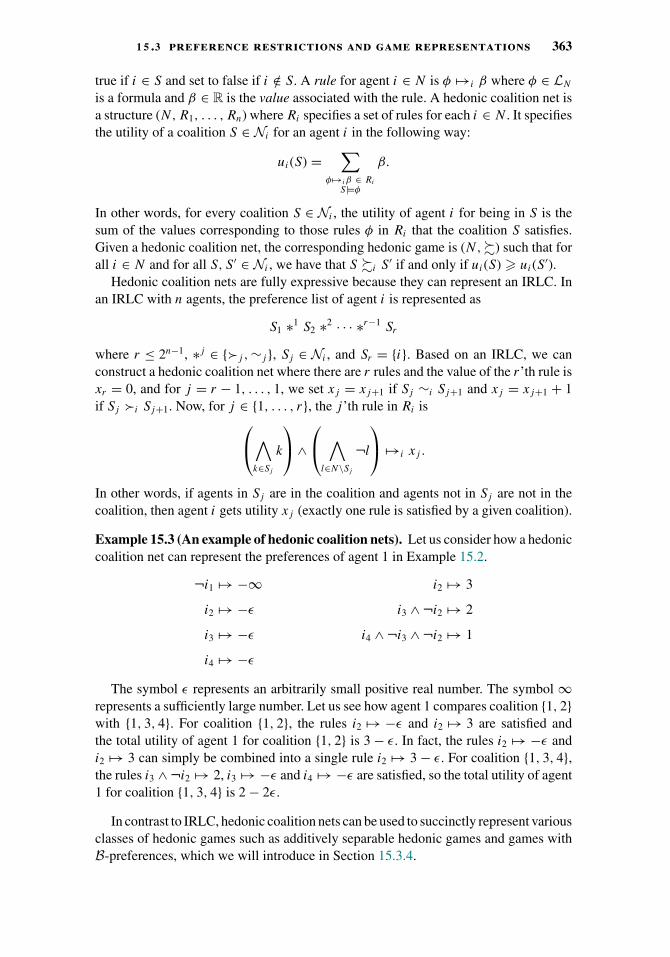
1 5 .3 preference restrictions and game representations 363
true if i ∈ S and set to false if i /∈ S. A rule for agent i ∈ N is φ �→i β where φ ∈ LN
is a formula and β ∈ R is the value associated with the rule. A hedonic coalition net isa structure (N, R1, . . . , Rn) where Ri specifies a set of rules for each i ∈ N . It specifiesthe utility of a coalition S ∈ Ni for an agent i in the following way:
ui(S) =∑
φ �→iβ ∈ Ri
S|=φ
β.
In other words, for every coalition S ∈ Ni , the utility of agent i for being in S is thesum of the values corresponding to those rules φ in Ri that the coalition S satisfies.Given a hedonic coalition net, the corresponding hedonic game is (N,�) such that forall i ∈ N and for all S, S ′ ∈ Ni , we have that S �i S ′ if and only if ui(S) � ui(S ′).
Hedonic coalition nets are fully expressive because they can represent an IRLC. Inan IRLC with n agents, the preference list of agent i is represented as
S1 ∗1 S2 ∗2 · · · ∗r−1 Sr
where r ≤ 2n−1, ∗j ∈ {�j ,∼j }, Sj ∈ Ni , and Sr = {i}. Based on an IRLC, we canconstruct a hedonic coalition net where there are r rules and the value of the r’th rule isxr = 0, and for j = r − 1, . . . , 1, we set xj = xj+1 if Sj ∼i Sj+1 and xj = xj+1 + 1if Sj �i Sj+1. Now, for j ∈ {1, . . . , r}, the j ’th rule in Ri is⎛⎝∧
k∈Sj
k
⎞⎠ ∧⎛⎝ ∧
l∈N\Sj
¬l
⎞⎠ �→i xj .
In other words, if agents in Sj are in the coalition and agents not in Sj are not in thecoalition, then agent i gets utility xj (exactly one rule is satisfied by a given coalition).
Example 15.3 (An example of hedonic coalition nets). Let us consider how a hedoniccoalition net can represent the preferences of agent 1 in Example 15.2.
¬i1 �→ −∞ i2 �→ 3
i2 �→ −ε i3 ∧ ¬i2 �→ 2
i3 �→ −ε i4 ∧ ¬i3 ∧ ¬i2 �→ 1
i4 �→ −ε
The symbol ε represents an arbitrarily small positive real number. The symbol ∞represents a sufficiently large number. Let us see how agent 1 compares coalition {1, 2}with {1, 3, 4}. For coalition {1, 2}, the rules i2 �→ −ε and i2 �→ 3 are satisfied andthe total utility of agent 1 for coalition {1, 2} is 3 − ε. In fact, the rules i2 �→ −ε andi2 �→ 3 can simply be combined into a single rule i2 �→ 3 − ε. For coalition {1, 3, 4},the rules i3 ∧ ¬i2 �→ 2, i3 �→ −ε and i4 �→ −ε are satisfied, so the total utility of agent1 for coalition {1, 3, 4} is 2 − 2ε.
In contrast to IRLC, hedonic coalition nets can be used to succinctly represent variousclasses of hedonic games such as additively separable hedonic games and games withB-preferences, which we will introduce in Section 15.3.4.
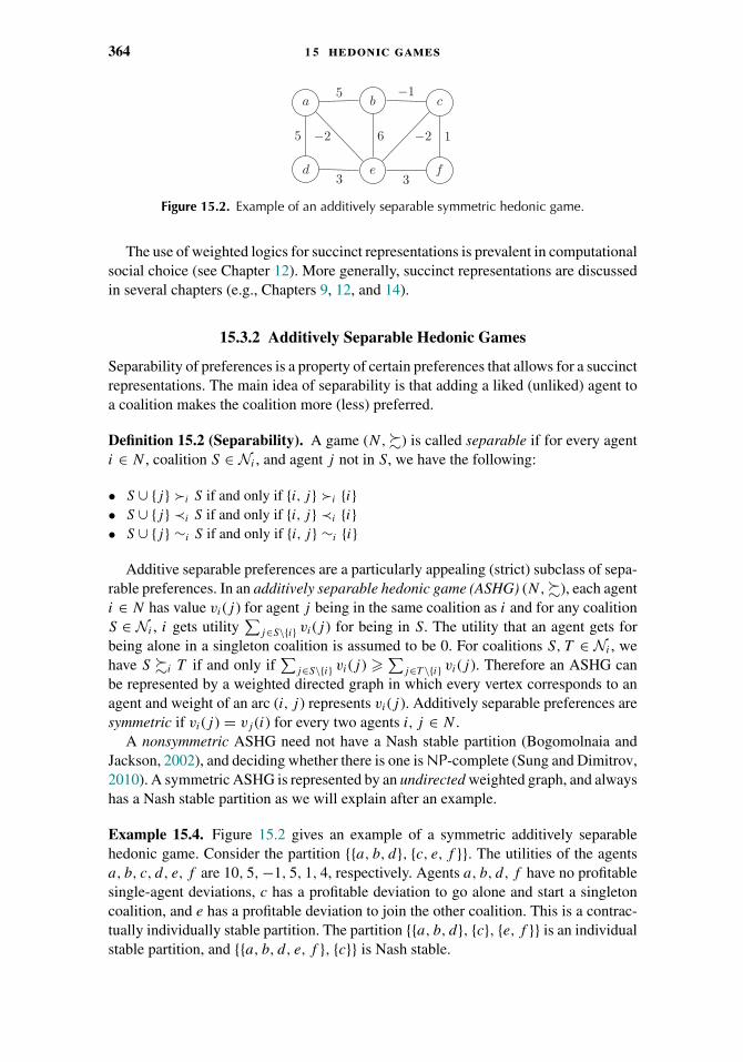
364 1 5 hedonic games
a b c
d e f
5 −1
5
3 3
16−2 −2
Figure 15.2. Example of an additively separable symmetric hedonic game.
The use of weighted logics for succinct representations is prevalent in computationalsocial choice (see Chapter 12). More generally, succinct representations are discussedin several chapters (e.g., Chapters 9, 12, and 14).
15.3.2 Additively Separable Hedonic Games
Separability of preferences is a property of certain preferences that allows for a succinctrepresentations. The main idea of separability is that adding a liked (unliked) agent toa coalition makes the coalition more (less) preferred.
Definition 15.2 (Separability). A game (N,�) is called separable if for every agenti ∈ N , coalition S ∈ Ni , and agent j not in S, we have the following:
• S ∪ {j} �i S if and only if {i, j} �i {i}• S ∪ {j} ≺i S if and only if {i, j} ≺i {i}• S ∪ {j} ∼i S if and only if {i, j} ∼i {i}
Additive separable preferences are a particularly appealing (strict) subclass of sepa-rable preferences. In an additively separable hedonic game (ASHG) (N,�), each agenti ∈ N has value vi(j ) for agent j being in the same coalition as i and for any coalitionS ∈ Ni , i gets utility
∑j∈S\{i} vi(j ) for being in S. The utility that an agent gets for
being alone in a singleton coalition is assumed to be 0. For coalitions S, T ∈ Ni , wehave S �i T if and only if
∑j∈S\{i} vi(j ) �∑
j∈T \{i} vi(j ). Therefore an ASHG canbe represented by a weighted directed graph in which every vertex corresponds to anagent and weight of an arc (i, j ) represents vi(j ). Additively separable preferences aresymmetric if vi(j ) = vj (i) for every two agents i, j ∈ N .
A nonsymmetric ASHG need not have a Nash stable partition (Bogomolnaia andJackson, 2002), and deciding whether there is one is NP-complete (Sung and Dimitrov,2010). A symmetric ASHG is represented by an undirected weighted graph, and alwayshas a Nash stable partition as we will explain after an example.
Example 15.4. Figure 15.2 gives an example of a symmetric additively separablehedonic game. Consider the partition {{a, b, d}, {c, e, f }}. The utilities of the agentsa, b, c, d, e, f are 10, 5,−1, 5, 1, 4, respectively. Agents a, b, d, f have no profitablesingle-agent deviations, c has a profitable deviation to go alone and start a singletoncoalition, and e has a profitable deviation to join the other coalition. This is a contrac-tually individually stable partition. The partition {{a, b, d}, {c}, {e, f }} is an individualstable partition, and {{a, b, d, e, f }, {c}} is Nash stable.

1 5 .3 preference restrictions and game representations 365
For an additively separable symmetric hedonic game, the existence of a Nash stable(NS) partition (and therefore also a CNS, CIS, and IS partition) is guaranteed byan argument based on a “potential function,” which was noted by Bogomolnaia andJackson (2002). We will construct an exact potential function. For every partition theexact potential function assigns a potential value equal to half the sum of agents’utilities under this partition. A deviation by a single agent from its coalition to anotherwill change the value of this potential function by exactly the change in the utility ofthis deviating agent (every edge gained or lost in the sum of agents’ utilities countstwice). Because the potential function is bounded, and there are finitely many partitions,and every profitable deviation by a single agent improves the value of the potentialfunction, we have the following: starting from any partition, every maximally longsequence of profitable deviations by agents terminates with a Nash stable partition.Note that symmetry is key for this potential function argument to work.
15.3.3 Games Based on the Best or Worst Agents
We now describe classes of hedonic games in which the agents’ preferences overcoalitions are induced by their ordinal preferences over the other individual agentsvia set extensions (Hajdukova, 2006; Barbera et al., 2004). Two of the most naturalways to extend preferences is based on the most preferred or least preferred agent inthe coalition. For a subset J of agents, we denote by max�i
(J ) and min�i(J ) the sets
of the most and least preferred agents in J by i, respectively. In B (where B standsfor best) and W (where W stands for worst) games each agent’s appreciation of acoalition depends on the most preferred (best) or least preferred (worst) agent in thecoalition. Note that roommate markets can also be considered in the framework withthe additional constraint that coalitions of size three or more are not feasible.
In hedonic games with B-preferences (which we will refer to as B-hedonic games),S �i T if and only if, we have either:
(i) for each s ∈ max�i(S \ {i}) and t ∈ max�i
(T \ {i}), s �i t , or(ii) for each s ∈ max�i
(S \ {i}) and t ∈ max�i(T \ {i}), s ∼i t and |S| < |T |.
So an agent’s appreciation of a coalition depends on its most favoured agents in thecoalition. If two coalitions have equally preferred agents, then a smaller coalition isstrictly preferred (Cechlarova and Hajdukova, 2002; Cechlarova and Romero-Medina,2001).
Example 15.5 (A B-hedonic game). Let (N,�) be a game with N = {1, 2, 3, 4} andlet the agents have preferences over other agents as follows:
2 �1 3 �1 4 �1 1,
3 �2 4 �2 1 �2 2,
1 �3 2 �3 4 �3 3,
3 �4 2 �4 1 �4 4.
For theB-hedonic game, the preferences of each agent over other agents are extendedover the preferences over sets of agents. The preferences of the agents are as follows
366 1 5 hedonic games
(the preference of agent 1 is the same as in Example 15.2). For brevity, we omit thecommas separating agents in each coalition.
{12} �1 {123} ∼1 {124} �1 {1234} �1 {13} �1 {134} �1 {14} �1 {1},{23} �2 {234} ∼2 {123} �2 {1234} �2 {24} �2 {124} �2 {12} �2 {2},{13} �3 {123} ∼3 {134} �3 {1234} �3 {23} �3 {234} �3 {34} �3 {3},{34} �4 {134} ∼4 {234} �4 {1234} �4 {24} �4 {124} �4 {14} �4 {4}.
In hedonic games withW-preferences (which we will refer to asW-hedonic games),S �i T if and only if for each s ∈ min�i
(S \ {i}) and t ∈ min�i(T \ {i}), we have
s �i t . So an agent’s appreciation of a coalition depends on its least preferred favouredagents in the coalition (Cechlarova and Hajdukova, 2004b; Cechlarova and Romero-Medina, 2001).
Other games can be defined based on preferences that depend on both the bestand worst agents in the coalition (Hajdukova, 2006) or in which the presence of anunacceptable agent in the coalition makes the coalition unacceptable (Aziz et al., 2012a,2013e). B-hedonic games, in which agents express strict preferences over other agents,are known to admit a core stable partition (Cechlarova and Romero-Medina, 2001).For further details on games based on the best or worst agents, we refer the reader toAziz et al. (2012a, 2013e); Cechlarova and Romero-Medina (2001); Cechlarova andHajdukova (2004b); Hajdukova (2006). B-hedonic games with strict preferences forma subclass of a larger class of hedonic games that satisfy top responsiveness.
15.3.4 Top Responsiveness
Identifying sufficient and necessary conditions for the existence of stability in coalitionformation has been a very active area of research. Perhaps the most celebrated result inthis field is the existence of a (core) stable matching for the stable marriage problem,which is shown constructively via the deferred-acceptance algorithm (Gale and Shap-ley, 1962). For hedonic games, more generally, a number of preference restrictions havebeen identified for which a stable partition is guaranteed to exist for some notion ofstability (see, e.g., Alcalde and Revilla, 2004; Aziz and Brandl, 2012; Banerjee et al.,2001; Bogomolnaia and Jackson, 2002; Dimitrov et al., 2006; Dimitrov and Sung,2007; Karakaya, 2011). In this subsection, we present an example of hedonic gamesthat satisfy top responsiveness (Alcalde and Revilla, 2004) that always admit a corestable partition.
Every coalition contains subset subcoalitions over which the agents also have prefer-ences. Top responsiveness captures the situation in which each agent’s appreciation ofa coalition depends on the most preferred subset within the coalition. If two coalitionshave the same most preferred subcoalition, then the coalition with the smaller size ispreferred. Top responsiveness is based on choice sets, which are sets of agents that anagent wants to be with. We use Ch(i, S) to denote the choice sets of agent i in coalitionS. It is formally defined as follows:
Ch(i, S) := {S ′ ⊆ S : (i ∈ S ′) ∧ (S ′ �i S ′′ ∀S ′′ ⊆ S)}.

1 5 .4 algorithms and computational complexity 367
If |Ch(i, S)| = 1, we denote by ch(i, S) the unique subset of S that is maximallypreferred by agent i on under �i : A game satisfies top responsiveness if |Ch(i, S)| = 1for each i ∈ N and S ∈ Ni and the following conditions hold for each i ∈ N and allS, T ∈ Ni ,
(i) S �i T if ch(i, S) �i ch(i, T );(ii) S �i T if ch(i, S) = ch(i, T ) and S ⊂ T .
Example 15.6 (An example of top responsive preferences). The hedonic gamespecified in Example 15.5 satisfies top responsiveness. For example, for agent 1, itschoice set of the grand coalition is {1, 2}. It likes each coalition that is a superset of{1, 2} more than any coalition that is not a superset of {1, 2}. Moreover, it prefers asmaller coalition that is a superset of {1, 2} more than a bigger coalition.
In Section 15.4.3, we show how to exploit the top responsiveness propertyalgorithmically.
15.4 Algorithms and Computational Complexity
In this section we give an overview of computational results concerning hedonicgames. For a given solution concept α, such as core stability, we consider the followingnatural computational problems:
Verification: Given (N,�) and a partition π of N , does π satisfy α?Existence: Given (N,�), does there exist a partition satisfying α?Construction: Given (N,�), if a partition satisfying α exists, find one.
15.4.1 Hardness to Check Non-emptiness of Core
We next consider the problem Existence for core stability for a hedonic game givenas an IRLC, which was shown by Ballester (2004) to be NP-complete.
Theorem 15.7 (Ballester, 2004). For hedonic games in IRLC, the problem of checkingwhether there exists a core stable partition is NP-complete.
Proof. Given an IRLC, Verification for core stability can be solved in polynomialtime because each agent explicitly lists all the individually rational coalitions, and theseare also all the potentially blocking coalitions. Thus the problem of deciding whethera core stable partition exists is in NP.
We now show that it is NP-hard and thus NP-complete, via a reduction fromExactCoverBy3Sets.
ExactCoverBy3Sets (X3C).Instance: Set X and set T that consists of 3-element subsets of X.Question: Does there exist a subset of T that partitions X?
We construct a hedonic game where N = {x, x ′, x ′′ : x ∈ X} and � is defined asfollows. For each i ∈ {x, x ′, x ′′}, let Xi
1, . . . , Xim be the elements in T such that they
include i.
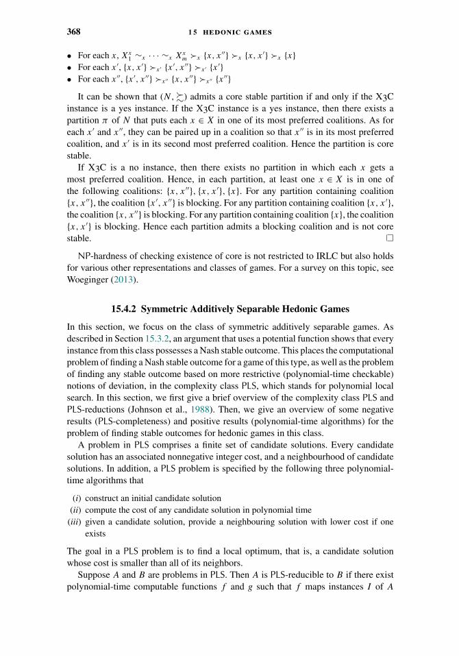
368 1 5 hedonic games
• For each x, Xx1 ∼x · · · ∼x Xx
m �x {x, x ′′} �x {x, x ′} �x {x}• For each x ′, {x, x ′} �x ′ {x ′, x ′′} �x ′ {x ′}• For each x ′′, {x ′, x ′′} �x ′′ {x, x ′′} �x ′′ {x ′′}
It can be shown that (N,�) admits a core stable partition if and only if the X3Cinstance is a yes instance. If the X3C instance is a yes instance, then there exists apartition π of N that puts each x ∈ X in one of its most preferred coalitions. As foreach x ′ and x ′′, they can be paired up in a coalition so that x ′′ is in its most preferredcoalition, and x ′ is in its second most preferred coalition. Hence the partition is corestable.
If X3C is a no instance, then there exists no partition in which each x gets amost preferred coalition. Hence, in each partition, at least one x ∈ X is in one ofthe following coalitions: {x, x ′′}, {x, x ′}, {x}. For any partition containing coalition{x, x ′′}, the coalition {x ′, x ′′} is blocking. For any partition containing coalition {x, x ′},the coalition {x, x ′′} is blocking. For any partition containing coalition {x}, the coalition{x, x ′} is blocking. Hence each partition admits a blocking coalition and is not corestable.
NP-hardness of checking existence of core is not restricted to IRLC but also holdsfor various other representations and classes of games. For a survey on this topic, seeWoeginger (2013).
15.4.2 Symmetric Additively Separable Hedonic Games
In this section, we focus on the class of symmetric additively separable games. Asdescribed in Section 15.3.2, an argument that uses a potential function shows that everyinstance from this class possesses a Nash stable outcome. This places the computationalproblem of finding a Nash stable outcome for a game of this type, as well as the problemof finding any stable outcome based on more restrictive (polynomial-time checkable)notions of deviation, in the complexity class PLS, which stands for polynomial localsearch. In this section, we first give a brief overview of the complexity class PLS andPLS-reductions (Johnson et al., 1988). Then, we give an overview of some negativeresults (PLS-completeness) and positive results (polynomial-time algorithms) for theproblem of finding stable outcomes for hedonic games in this class.
A problem in PLS comprises a finite set of candidate solutions. Every candidatesolution has an associated nonnegative integer cost, and a neighbourhood of candidatesolutions. In addition, a PLS problem is specified by the following three polynomial-time algorithms that
(i) construct an initial candidate solution(ii) compute the cost of any candidate solution in polynomial time
(iii) given a candidate solution, provide a neighbouring solution with lower cost if oneexists
The goal in a PLS problem is to find a local optimum, that is, a candidate solutionwhose cost is smaller than all of its neighbors.
Suppose A and B are problems in PLS. Then A is PLS-reducible to B if there existpolynomial-time computable functions f and g such that f maps instances I of A

1 5 .4 algorithms and computational complexity 369
to instances f (I ) of B, and g maps the local optima of instances f (I ) of B to localoptima of instance I . A problem in PLS is PLS-complete if all problems in PLS arePLS-reducible to it. PLS captures the problem of finding pure Nash equilibria for manyclasses of games where pure equilibria are guaranteed to exist, such as congestiongames Fabrikant et al. (2004).
On one hand, it is very unlikely that a PLS problem is NP-hard because this wouldimply NP = coNP (Johnson et al., 1988). On the other hand, a polynomial-timealgorithm for a PLS-complete problem would resolve a number of long open problems,for example, because it would show that simple stochastic games can be solved inpolynomial time (Yannakakis, 2008). Thus, PLS-complete problems are believed notto admit polynomial-time algorithms.
Observation 15.8 (Gairing and Savani, 2010). For symmetric additively separablehedonic games, Construction for Nash Stability is PLS-complete.
Proof. We reduce from the PLS-complete problem PartyAffiliation, which is tocompute an equilibrium of a party affiliation game. The input of PartyAffiliationis an undirected edge-weighted graph. A solution is a partition of the nodes into twoparties such that for every node v the sum of edge weights of edges from v to othernodes in v’s part is greater that the sum of edge weights to nodes in the other party.A party affiliation game is essentially a symmetric additively separable hedonic gamewhere at most two coalitions are permitted.
Consider an instance G = (V, E, w) of PartyAffiliation. We augment G byintroducing two new agents, called super nodes. Every agent i ∈ V has an edge, ofweight W >
∑e∈E |we|, to each of the super nodes. The two super nodes are connected
by an edge of weight −M , where M > |V | · W . Use the resulting graph to define acorresponding hedonic additively separable game and consider Nash stable outcomes.By the choice of M the two super nodes will be in different coalitions in any Nash stableoutcome of the resulting hedonic game. Moreover, by the choice of W , each agent willbe in a coalition with one of the super nodes. So, in each Nash stable outcome we haveexactly two coalitions. The fact that edges to super nodes have all the same weightdirectly implies a one-to-one correspondence between the Nash stable outcomes in thehedonic game and in the party affiliation game.
Every Nash stable outcome is also an individually stable outcome and thusConstruction is no harder for individual stability than for Nash stability. It turnsout that Construction for individual stability is still PLS-hard, though the simplestreduction we know that shows this result is much more involved than the proof of Obser-vation 15.8 for Nash stability (Gairing and Savani, 2010, 2011). When deviations ofplayers are restricted even further, and we move from individual stability to contractualindividual stability, the problem Construction becomes efficiently solvable:
Observation 15.9 (Gairing and Savani, 2010). For symmetric additively separablehedonic games, Construction for CIS can be solved in O(|E|) time. Moreover, localimprovements converge in at most 2|V | steps.
Proof. Consider the following algorithm to solve the game G = (V, E, w):
Delete all negative edges from G and put every connected component in a separate coalition.

370 1 5 hedonic games
Consider any coalition formed by this algorithm. If the coalition consists of only oneagent, then this agent has no positive edges to any agent and staying alone is a (weakly)dominant strategy. Agents in larger coalitions are connected by a positive edge to someagent within the same coalition. Therefore, they are not allowed to leave the coalition.Thus, we have computed a CIS stable state. Finding the connected components of anundirected graph can be done by depth-first search in O(|E|) time.
Now consider local improvements. Observe that whenever an agent joins a non-empty coalition then this agent (and all agents to which it is connected by a positiveedge in the coalition) will never move again. Moreover, an agent can only start a newcoalition once. It follows that each agent can make at most two strategy changes. Intotal we have at most 2|V | local improvements.
For further results on additively separable hedonic games, we refer the reader toAziz et al. (2013b), Sung and Dimitrov (2010), Olsen (2009), and Sung and Dimitrov(2007a).
15.4.3 Top Covering Algorithm
In Section 15.3.4, we discussed games that satisfy top responsiveness that are guaran-teed to admit a core stable partition. Next, we define the Top Covering Algorithm to com-pute a core stable partition for hedonic games satisfying top responsiveness (Alcaldeand Revilla, 2004; Dimitrov and Sung, 2006). For this we need the following defi-nitions. For each X ⊆ N , we denote by �X the relation on X × X where i �X j ifand only if j ∈ ch(i, X). In this case j is called a neighbour of i in X. The connectedcomponent CC(i, X) of i with respect to X is defined as follows:
CC(i, X) = {k ∈ X : ∃j1, . . . , jl ∈ X : i = j1 �X · · · �X jl = k}.Based on the concept of connected components, we can specify the Top Covering Algo-rithm. The algorithm is formally specified as Algorithm 1 and is based on similar ideasas that of the Top Trading Cycle Algorithm for exchange of indivisible objects (Shapleyand Scarf, 1974). We maintain a partition π and a set Rk as the set of remaining agentsin round k. In each round, an agent i is selected from Rk for which the size of theconnected component of i with respect to Rk is at most the size of the connected com-ponent of some other agent j ∈ Rk with respect to Rk . Such a connected component isa new coalition in partition π . The process is iterated until no more agents remain. Forhedonic games that satisfy top responsiveness, the Top Covering Algorithm returns acore stable partition. Alcalde and Revilla (2004) also proved that, for top responsivepreferences, the Top Covering Algorithm is strategyproof. If the preference profilesatisfies some natural constraints in addition to top responsiveness, the Top CoveringAlgorithm returns a partition which satisfies even stronger notions of stability than corestability (Aziz and Brandl, 2012).
Example 15.10 (An example illustrating the Top Covering Algorithm). Werun the Top Covering Algorithm on the hedonic game specified in Example 15.5.Example 15.6 pointed out that the hedonic game satisfies top responsiveness. First, weexamine the connected components. Initially, R1 = {1, 2, 3, 4}, CC(1, {1, 2, 3, 4}) =
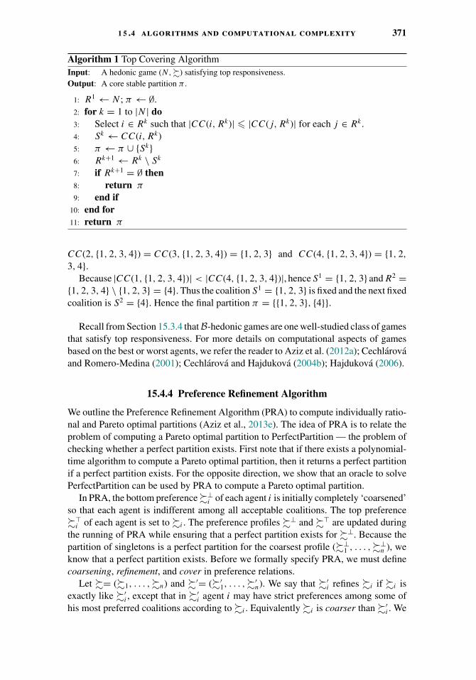
1 5 .4 algorithms and computational complexity 371
Algorithm 1 Top Covering AlgorithmInput: A hedonic game (N,�) satisfying top responsiveness.Output: A core stable partition π .
1: R1 ← N ; π ← ∅.2: for k = 1 to |N | do3: Select i ∈ Rk such that |CC(i, Rk)| � |CC(j, Rk)| for each j ∈ Rk .4: Sk ← CC(i, Rk)5: π ← π ∪ {Sk}6: Rk+1 ← Rk \ Sk
7: if Rk+1 = ∅ then8: return π
9: end if10: end for11: return π
CC(2, {1, 2, 3, 4}) = CC(3, {1, 2, 3, 4}) = {1, 2, 3} and CC(4, {1, 2, 3, 4}) = {1, 2,
3, 4}.Because |CC(1, {1, 2, 3, 4})| < |CC(4, {1, 2, 3, 4})|, hence S1 = {1, 2, 3} and R2 =
{1, 2, 3, 4} \ {1, 2, 3} = {4}. Thus the coalition S1 = {1, 2, 3} is fixed and the next fixedcoalition is S2 = {4}. Hence the final partition π = {{1, 2, 3}, {4}}.
Recall from Section 15.3.4 thatB-hedonic games are one well-studied class of gamesthat satisfy top responsiveness. For more details on computational aspects of gamesbased on the best or worst agents, we refer the reader to Aziz et al. (2012a); Cechlarovaand Romero-Medina (2001); Cechlarova and Hajdukova (2004b); Hajdukova (2006).
15.4.4 Preference Refinement Algorithm
We outline the Preference Refinement Algorithm (PRA) to compute individually ratio-nal and Pareto optimal partitions (Aziz et al., 2013e). The idea of PRA is to relate theproblem of computing a Pareto optimal partition to PerfectPartition — the problem ofchecking whether a perfect partition exists. First note that if there exists a polynomial-time algorithm to compute a Pareto optimal partition, then it returns a perfect partitionif a perfect partition exists. For the opposite direction, we show that an oracle to solvePerfectPartition can be used by PRA to compute a Pareto optimal partition.
In PRA, the bottom preference�⊥i of each agent i is initially completely ‘coarsened’
so that each agent is indifferent among all acceptable coalitions. The top preference�(
i of each agent is set to �i . The preference profiles �⊥ and �( are updated duringthe running of PRA while ensuring that a perfect partition exists for �⊥. Because thepartition of singletons is a perfect partition for the coarsest profile (�⊥
1 , . . . ,�⊥n ), we
know that a perfect partition exists. Before we formally specify PRA, we must definecoarsening, refinement, and cover in preference relations.
Let �= (�1, . . . ,�n) and �′= (�′1, . . . ,�′
n). We say that �′i refines �i if �i is
exactly like �′i , except that in �′
i agent i may have strict preferences among some ofhis most preferred coalitions according to �i . Equivalently �i is coarser than �′
i . We
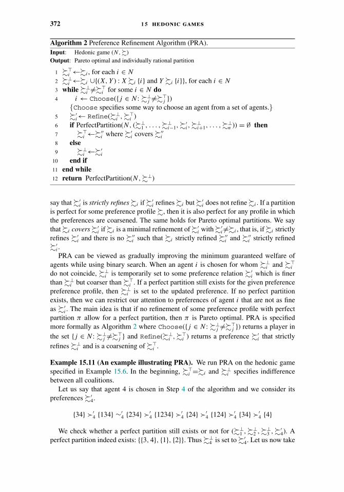
372 1 5 hedonic games
Algorithm 2 Preference Refinement Algorithm (PRA).Input: Hedonic game (N,�)Output: Pareto optimal and individually rational partition
1 �(i ←�i , for each i ∈ N
2 �⊥i ←�i ∪{(X, Y ) : X�i {i} and Y �i {i}}, for each i ∈ N
3 while �⊥i �=�(
i for some i ∈ N do4 i ← Choose({j ∈ N : �⊥
j �=�(j })
{Choose specifies some way to choose an agent from a set of agents.}5 �′
i← Refine(�⊥i ,�(
i )6 if PerfectPartition(N, (�⊥
1 , . . . ,�⊥i−1,�′
i ,�⊥i+1, . . . ,�⊥
n )) = ∅ then7 �(
i ←�′′i where �′
i covers �′′i
8 else9 �⊥
i ←�′i
10 end if11 end while12 return PerfectPartition(N,�⊥)
say that �′i is strictly refines �i if �′
i refines �i but �′i does not refine �i . If a partition
is perfect for some preference profile �, then it is also perfect for any profile in whichthe preferences are coarsened. The same holds for Pareto optimal partitions. We saythat �i covers �′
i if �i is a minimal refinement of �′i with �′
i �=�i , that is, if �i strictlyrefines �′
i and there is no �′′i such that �i strictly refined �′′
i and �′′i strictly refined
�′i .PRA can be viewed as gradually improving the minimum guaranteed welfare of
agents while using binary search. When an agent i is chosen for whom �⊥i and �(
i
do not coincide, �⊥i is temporarily set to some preference relation �′
i which is finerthan �⊥
i but coarser than �(i . If a perfect partition still exists for the given preference
preference profile, then �⊥i is set to the updated preference. If no perfect partition
exists, then we can restrict our attention to preferences of agent i that are not as fineas �′
i . The main idea is that if no refinement of some preference profile with perfectpartition π allow for a perfect partition, then π is Pareto optimal. PRA is specifiedmore formally as Algorithm 2 where Choose({j ∈ N : �⊥
j �=�(j }) returns a player in
the set {j ∈ N : �⊥j �=�(
j } and Refine(�⊥i ,�(
i ) returns a preference �′i that strictly
refines �⊥i and is a coarsening of �(
i .
Example 15.11 (An example illustrating PRA). We run PRA on the hedonic gamespecified in Example 15.6. In the beginning, �(
i =�i and �⊥i specifies indifference
between all coalitions.Let us say that agent 4 is chosen in Step 4 of the algorithm and we consider its
preferences �′4.
{34} �′4 {134} ∼′
4 {234} �′4 {1234} �′
4 {24} �′4 {124} �′
4 {34} �′4 {4}
We check whether a perfect partition still exists or not for (�⊥1 ,�⊥
2 ,�⊥3 ,�′
4). Aperfect partition indeed exists: {{3, 4}, {1}, {2}}. Thus �⊥
4 is set to �′4. Let us now take

1 5 .5 further reading 373
agent 2 and consider its preference �′2.
{23} ∼′2 {234} ∼′
2 {213} ∼′2 {1234} ∼′
2 {24} ∼′2 {214} �′
2 {12} �′2 {2}
However, no perfect partition exists for (�⊥1 ,�′
2,�⊥3 ,�⊥
4 ). Hence �(2 is changed
as follows:
{23} ∼(2 {234} ∼(
2 {213} ∼(2 {1234} ∼(
2 {24} ∼(2 {214} ∼(
2 {12} �(2 {2}
The process goes on until top and bottom preferences of the agents are as followsin the end:
{12} �⊥1 {123} ∼⊥
1 {124} �⊥1 {1234} �⊥
1 {13} �⊥1 {134} �⊥
1 {14} �⊥1 {1},
{23} ∼⊥2 {234} ∼⊥
2 {213} ∼⊥2 {1234} ∼⊥
2 {24} ∼⊥2 {214} ∼⊥
2 {12},{13} ∼⊥
3 {123} ∼⊥3 {134} ∼⊥
3 {1234} ∼⊥3 {23} ∼⊥
3 {234} ∼⊥3 {34} �⊥
3 {3},{34} �⊥
4 {134} ∼⊥4 {234} �⊥
4 {1234} �⊥4 {24} �⊥
4 {124} �⊥4 {14} �⊥
4 {4}.The perfect partition for (�⊥
1 ,�⊥2 ,�⊥
3 ,�⊥4 ) = (�(
1 ,�(2 ,�(
3 ,�(4 ) is {{3, 4}, {1, 2}}.
which is Pareto optimal for �.
Any Pareto optimal and individually rational partition can be returned by PRAdepending on how the refinements of preferences are carried out. The behaviour ofPRA may depend on the specific settings of Choose and Refine. In particular thefollowing are two interesting versions of PRA. In PRASD, Choose selects playersaccording to a fixed order of the players and Refine returns a player’s finest preferencerelation, that is, generally Refine(�⊥
i ,�(i )= �(
i . In PRAEgal, Choose selects aplayer that has been selected the fewest number of times during the execution of PRA.Refine is defined such that Refine(�⊥
i ,�(i ) = Cover(Q⊥
i ). Both versions have theirmerits. If all coalitions are acceptable then PRASD is strategyproof. On the other hand,PRAEgal satisfies the following property: for any k ∈ N for which there exists a Paretooptimal partition in which none of the players get one of their kth lowest-ranked orworse coalitions, PRAEgal will return such a partition.
PRA can be adapted for various specific classes of hedonic games by formulatingspecific algorithms to solve PerfectPartition for those classes. For example, applyingthis idea yields a polynomial-time algorithm to compute a Pareto optimal partition forW-hedonic games (Aziz et al., 2013e).
15.5 Further Reading
There are a number of topics that we have not touched on in this chapter. We havenot discussed strategic issues in detail (see, e.g., Demange, 2009). One reason is thatimpossibility results hold even for restricted classes of hedonic games (Barbera andGerber, 2007; Rodrıguez-Alvarez, 2009).
Various classes of hedonic games can be represented by graphs. Some of them arespecial subclasses of additively separable hedonic games, which we have discussed.An additively separable hedonic game (N, v) is an appreciation of friends game if forall i, j ∈ N such that i �= j , vi(j ) ∈ {−1,+n}. It is an aversion to enemies game if
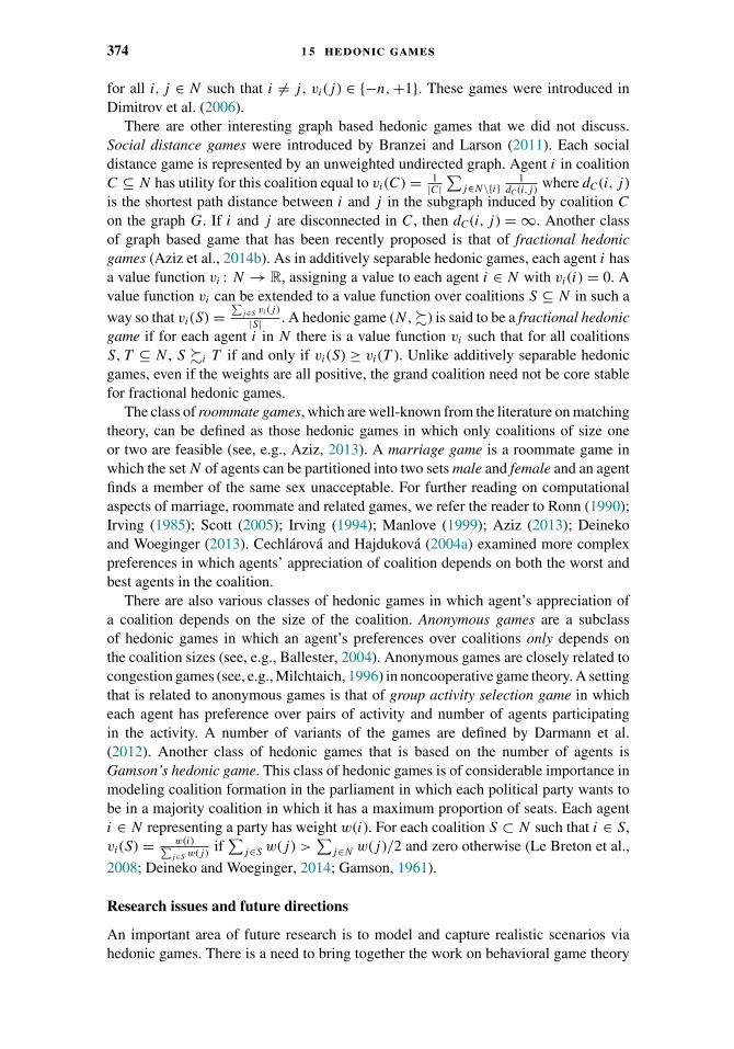
374 1 5 hedonic games
for all i, j ∈ N such that i �= j , vi(j ) ∈ {−n,+1}. These games were introduced inDimitrov et al. (2006).
There are other interesting graph based hedonic games that we did not discuss.Social distance games were introduced by Branzei and Larson (2011). Each socialdistance game is represented by an unweighted undirected graph. Agent i in coalitionC ⊆ N has utility for this coalition equal to vi(C) = 1
|C|∑
j∈N\{i}1
dC (i,j ) where dC(i, j )is the shortest path distance between i and j in the subgraph induced by coalition C
on the graph G. If i and j are disconnected in C, then dC(i, j ) = ∞. Another classof graph based game that has been recently proposed is that of fractional hedonicgames (Aziz et al., 2014b). As in additively separable hedonic games, each agent i hasa value function vi : N → R, assigning a value to each agent i ∈ N with vi(i) = 0. Avalue function vi can be extended to a value function over coalitions S ⊆ N in such a
way so that vi(S) =∑
j∈S vi (j )|S| . A hedonic game (N,�) is said to be a fractional hedonic
game if for each agent i in N there is a value function vi such that for all coalitionsS, T ⊆ N , S �i T if and only if vi(S) ≥ vi(T ). Unlike additively separable hedonicgames, even if the weights are all positive, the grand coalition need not be core stablefor fractional hedonic games.
The class of roommate games, which are well-known from the literature on matchingtheory, can be defined as those hedonic games in which only coalitions of size oneor two are feasible (see, e.g., Aziz, 2013). A marriage game is a roommate game inwhich the set N of agents can be partitioned into two sets male and female and an agentfinds a member of the same sex unacceptable. For further reading on computationalaspects of marriage, roommate and related games, we refer the reader to Ronn (1990);Irving (1985); Scott (2005); Irving (1994); Manlove (1999); Aziz (2013); Deinekoand Woeginger (2013). Cechlarova and Hajdukova (2004a) examined more complexpreferences in which agents’ appreciation of coalition depends on both the worst andbest agents in the coalition.
There are also various classes of hedonic games in which agent’s appreciation ofa coalition depends on the size of the coalition. Anonymous games are a subclassof hedonic games in which an agent’s preferences over coalitions only depends onthe coalition sizes (see, e.g., Ballester, 2004). Anonymous games are closely related tocongestion games (see, e.g., Milchtaich, 1996) in noncooperative game theory. A settingthat is related to anonymous games is that of group activity selection game in whicheach agent has preference over pairs of activity and number of agents participatingin the activity. A number of variants of the games are defined by Darmann et al.(2012). Another class of hedonic games that is based on the number of agents isGamson’s hedonic game. This class of hedonic games is of considerable importance inmodeling coalition formation in the parliament in which each political party wants tobe in a majority coalition in which it has a maximum proportion of seats. Each agenti ∈ N representing a party has weight w(i). For each coalition S ⊂ N such that i ∈ S,vi(S) = w(i)∑
j∈S w(j ) if∑
j∈S w(j ) >∑
j∈N w(j )/2 and zero otherwise (Le Breton et al.,
2008; Deineko and Woeginger, 2014; Gamson, 1961).
Research issues and future directions
An important area of future research is to model and capture realistic scenarios viahedonic games. There is a need to bring together the work on behavioral game theory
1 5 .5 further reading 375
and mathematical game theory. This may help identify other interesting classes ofhedonic games and preference restrictions. Identifying other natural set extensions forcompact representations of hedonic games will be fruitful.
Another issue is that in many realistic scenarios, most agents are part of overlappingcoalitions. Although there is interesting work on overlapping coalitions in transferableutility cooperative game theory (see, e.g., Chalkiadakis et al., 2010), there is scope formore work on overlapping coalitions in hedonic games. We have focussed on outcomesin which each agent is in one of the coalitions of the partition. The setting can be gen-eralized to allow agents to be partial members of various coalitions. This could, forexample, represent the proportion of time different coalitions are formed. Formally,a fractional hypergraph matching is a function w assigning nonnegative weights tocoalitions such that
∑S∈Ni
w(S) � 1 for all i ∈ N . A fractional hypergraph match-ing is stable if for every S ∈ 2N , there exists an i ∈ S such that
∑i∈T ∈Ni
T�iS
w(T ) = 1.
Aharoni and Fleiner (2003) used a connection with Scarf’s Lemma to show that a stablefractional hypergraph matching is guaranteed to exist. In general, the complexity ofcomputing a fractional stable matching is PPAD-complete (Kintali et al., 2009). Thereare other ways to define stability for fractional hypergraph matchings (Manjunath,2013) and each of the concepts leads to corresponding computational problems.
Although hedonic games have been examined computationally, their algorithmictreatment has been somewhat piecemeal. The hope is to come up with general algo-rithms that are not tailor-made for a specific representation of hedonic games and cancompute solutions of different classes of games. A plethora of intractability resultsindicates that a fixed parameter tractability approach (Niedermeier, 2006) may also befruitful. Finding faster exact exponential algorithms is also a natural avenue (Fominand Kratsch, 2010). Another research direction is to have logical representations ofhedonic games and propose logical characterizations of solution concepts which wouldenable SAT solvers to compute stable partitions (see, e.g., Aziz et al., 2014a). Finally,given that it is computationally hard to find many types of (exactly) stable outcomes, itis natural to study the computational complexity of finding approximately stable parti-tions. A first step in this direction for cut and party affiliation games, which are closelyrelated to additively separable hedonic games, was taken by Bhalgat et al. (2010).
Characterizing conditions under which stable partitions are guaranteed to existis one of the main research questions concerning hedonic games. Although varioussufficient conditions have been identified in the literature, there is scope for a betterunderstanding of sufficient and necessary conditions. Another interesting question isstudying the conditions under which a game has a unique stable partition. Papai (2004)characterized conditions under which a hedonic game has a unique core stable partition.There are various interesting questions regarding the complexity of checking whetherthe game has a unique core stable partition. It is not clear whether this question is easieror harder than checking the existence of a core stable partition.
Deviation dynamics in uncoordinated matching markets have been examined withincomputer science (see, e.g., Ackermann et al., 2011). The rich landscape of hedonicgames provides fertile ground for interesting research on dynamics of deviations.
Finally, the solutions of hedonic games based on graphs can be used as desirableways to perform network clustering and community detection (Aziz et al., 2014b; Olsen,2013). Aziz et al. (2014b) suggested core stable and welfare-maximizing partitions

376 1 5 hedonic games
of the fractional hedonic game corresponding to the graph as an interesting way ofclustering the vertices of the network. Further work (see, e.g., Bilo et al., 2014) in thisarea may be of interest to other communities working in network analysis (McSweeneyet al., 2014).
Acknowledgments
The authors acknowledge Martin Aleksandrov, Sajid Aziz, Felix Brandt, VinceConitzer, Paul Harrenstein, Jerome Lang, Dominik Peters, and Gerhard Woegingerfor their helpful and constructive comments. The authors acknowledge numerous use-ful discussions with Florian Brandl, Felix Brandt, Martin Gairing, Paul Harrenstein,and Hans Georg Seedig and thank them for their permission to adapt material fromjoint papers for this chapter. NICTA is funded by the Australian government throughthe Department of Communications and the Australian Research Council through theICT Centre of Excellence Program. Rahul Savani would like to acknowledge supportfrom the EPSRC under grant EP/L011018/1.
CHAPTER 16
Weighted Voting Games
Georgios Chalkiadakis and Michael Wooldridge
16.1 Introduction
In this chapter, we consider weighted voting games: a form of social choice systemthat seems much simpler than most schemes considered in this handbook, but whichis, nevertheless, widely used for many important real-world social choice problems.There are at least two very good reasons for studying weighted voting systems: first,as we have already mentioned, they are widely used in practice; and second, for alltheir apparent simplicity, they possess interesting mathematical and computationalproperties, making them interesting objects from the point of view of scientific study.
Weighted voting games originated in the domain of cooperative game the-ory (Chalkiadakis et al., 2011). They model decision-making situations in which aset of voters must make a binary (yes/no) decision on some particular issue; eachvoter is allocated a numeric weight, and the decision is carried if the sum of weightsof voters in favour of it meets or exceeds some specific given threshold, called thequota. Weighted voting games have many applications beyond social choice theory.For example, they can be used to model settings where each player has a certain amountof a given resource (say, time, money, or manpower), and there is a goal that can bereached by any coalition that possesses a sufficient amount of this resource.
The remainder of this chapter is structured as follows.
� In Section 16.2, we present the basic models and solution concepts that will be usedthroughout the remainder of the chapter. We start by defining cooperative games incharacteristic function form, and then introduce weighted voting games. We go on todescribe some key solution concepts for cooperative games: the core, the Shapley value,and the Banzhaf index.
� In Section 16.3, we consider computational properties of weighted voting games: inparticular, the complexity of computing the core, the Shapley value, and the Banzhafindex.
� In Section 16.4, we consider the (sometimes unintuitive) relationship between the weightthat a voter is assigned in a weighted voting game and the power that this voter thenwields.
377
378 1 6 weighted voting games
� In Section 16.5, we consider the extent to which weighted voting games can be consideredas a representation scheme for yes/no voting systems (i.e., simple cooperative games).We give a condition on yes/no voting systems that is both necessary and sufficient forsuch a system to be representable as a weighted voting game.
Throughout the chapter, we assume familiarity with the basic notation and terminologyof computational complexity theory (big-O notation, the classes P, NP, coNP, and#P) (Garey and Johnson, 1979; Papadimitriou, 1994).
16.2 Basic Definitions
Weighted voting games are a special case of a class of cooperative games, and the solu-tion concepts that we consider for weighted voting games are in fact those developedwithin cooperative game theory. In this section, we begin by presenting the key gamemodel from cooperative game theory, and then introduce weighted voting games as aspecial case of such game. We then define the key solution concepts for such games.
16.2.1 Cooperative Games
We start by defining the game model that underpins weighted voting games: formally,these are cooperative games with transferable utility in characteristic function form,but we will refer to them as cooperative games.
Definition 16.1. A cooperative game, G, is given by a pair G = (N, v), where N ={1, . . . , n} is the set of players of the game, and v : 2N → R is the characteristicfunction of the game. Unless otherwise stated, we assume that v(∅) = 0, and moreoverthat v({i}) = 0 for all i ∈ N . We will say a cooperative game G = (N, v) is simple ifv(C) ∈ {0, 1} for all C ⊆ N , in which case we say C ⊆ N are winning if v(C) = 1,and losing otherwise. A simple game is nontrivial if v(N) = 1. We will usually assumegames are nontrivial.
The basic idea behind this model is that any subset C ⊆ N of the players can cooperatewith each other, and, by joining forces, they can obtain the value v(C). The modeldoes not specify how the players cooperate; it only specifies what value they couldobtain through cooperation. It is conventional to refer to (sub)sets of players C ⊆ N
as coalitions: in everyday use the term “coalition” implies a collection of people withsome common cause or commitment to joint action, but we will mean it simply in thesense of a set of players, who may or may not choose to cooperate. We will refer to theset of all players N as the grand coalition.
16.2.2 Weighted Voting Games
We are now ready to define weighted voting games. A weighted voting game is a simplecooperative game (i.e., a game in which every coalition has a value of either 0 or 1),which is defined by each player in the game having a weight, and where a coalitionobtains the value 1 if the sum of their values meets or exceeds a given quota. Formally:
1 6 .2 basic definitions 379
Definition 16.2. A weighted voting game G with a set of players N = {1, . . . , n} isgiven by a list of weights w = (w1, . . . , wn) ∈ Rn and a quota q ∈ R; we will writeG = [N ; w; q]. The characteristic function v : 2N → {0, 1} of the game is defined asfollows:
v(C) ={
1 if∑
i∈C wi � q
0 otherwise.
We write w(C) to denote the total weight of a coalition C, that is, we set w(C) =∑i∈C wi . It is usually assumed that all weights and the quota are nonnegative; in what
follows, we will make this assumption as well. Under this assumption, weighted votinggames are monotone: if a coalition wins, then adding players to the coalition cannot turnit into a losing coalition. It is common to assume that 0 < q ≤ w(N); this conditionensures that the empty coalition is losing and the grand coalition is winning (and hencethe game is nontrivial).
Our definition of weighted voting games allows for arbitrary real number weights.However, it is not clear how to efficiently store and manipulate such weights, whichpresents a difficulty from the algorithmic point of view. Fortunately, it turns out thatany weighted voting game is equivalent to a game with fairly small integer weights.More precisely, we have the following theorem, which follows from results on linearthreshold functions (Muroga, 1971).
Theorem 16.1. Let us say two weighted voting games G = [N ; w; q] and G′ =[N ; w′; q ′] are equivalent iff for all coalitions C ⊆ N we have w(C) � q iff w′(C) � q ′.Then, for any weighted voting game G = [N ; w; q] with |N | = n, there exists an equiv-alent weighted voting game G′ = [N ; w′; q ′] with w′ = (w′
1, . . . , w′n) such that all w′
i ,i = 1, . . . , n, and q ′ are nonnegative integers, and w′
i = O(2n log n) for all i = 1, . . . , n.
We can therefore assume without loss of generality that all weights and the quotaare integers given in binary. We remark that, even though the entries of the weightvector w′ are exponential in n, they can be represented using O(n log n) bits—that is,a weighted voting game with n players can be described using poly(n) bits. Thus, anyweighted voting game has an equivalent “compact” representation: this fact is usefulwhen considering questions relating to computational complexity.
Before proceeding, let us say a few words about the applications of weighted votinggames. These games can be used to describe many real-world situations. In particular,they are very well suited to model coalition formation in legislative bodies. In moredetail, each party in a parliament can be associated with a player in a weighted votinggame; the weight of the player is given by the total number of the representatives of thisparty. The quota corresponds to the number of votes needed to pass a bill; while in mostcases a simple majority q = !w(N)/2" + 1 suffices, in some circumstances a bill canonly be passed if it is supported by two thirds of the legislators (i.e., q = 2w(N)/3),or even the entire legislative body (q = w(N)). Another example of a weighted votinggame is shareholder voting: the weight of each voter is proportional to the number ofshares she holds. A weighted voting game also arises in a setting where there is a taskthat requires q hours of work, and there is a group of agents N = {1, . . . , n} such thateach agent i can dedicate wi of his time to this task.
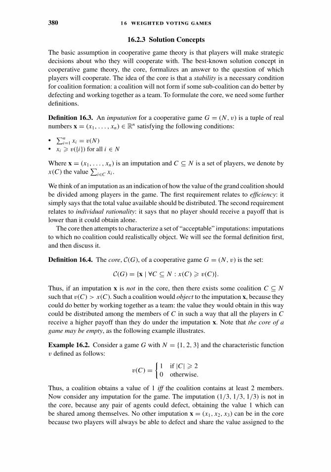
380 1 6 weighted voting games
16.2.3 Solution Concepts
The basic assumption in cooperative game theory is that players will make strategicdecisions about who they will cooperate with. The best-known solution concept incooperative game theory, the core, formalizes an answer to the question of whichplayers will cooperate. The idea of the core is that a stability is a necessary conditionfor coalition formation: a coalition will not form if some sub-coalition can do better bydefecting and working together as a team. To formulate the core, we need some furtherdefinitions.
Definition 16.3. An imputation for a cooperative game G = (N, v) is a tuple of realnumbers x = (x1, . . . , xn) ∈ Rn satisfying the following conditions:
�
∑ni=1 xi = v(N )
� xi � v({i}) for all i ∈ N
Where x = (x1, . . . , xn) is an imputation and C ⊆ N is a set of players, we denote byx(C) the value
∑i∈C xi .
We think of an imputation as an indication of how the value of the grand coalition shouldbe divided among players in the game. The first requirement relates to efficiency: itsimply says that the total value available should be distributed. The second requirementrelates to individual rationality: it says that no player should receive a payoff that islower than it could obtain alone.
The core then attempts to characterize a set of “acceptable” imputations: imputationsto which no coalition could realistically object. We will see the formal definition first,and then discuss it.
Definition 16.4. The core, C(G), of a cooperative game G = (N, v) is the set:
C(G) = {x | ∀C ⊆ N : x(C) � v(C)}.Thus, if an imputation x is not in the core, then there exists some coalition C ⊆ N
such that v(C) > x(C). Such a coalition would object to the imputation x, because theycould do better by working together as a team: the value they would obtain in this waycould be distributed among the members of C in such a way that all the players in C
receive a higher payoff than they do under the imputation x. Note that the core of agame may be empty, as the following example illustrates.
Example 16.2. Consider a game G with N = {1, 2, 3} and the characteristic functionv defined as follows:
v(C) ={
1 if |C| � 20 otherwise.
Thus, a coalition obtains a value of 1 iff the coalition contains at least 2 members.Now consider any imputation for the game. The imputation (1/3, 1/3, 1/3) is not inthe core, because any pair of agents could defect, obtaining the value 1 which canbe shared among themselves. No other imputation x = (x1, x2, x3) can be in the corebecause two players will always be able to defect and share the value assigned to the
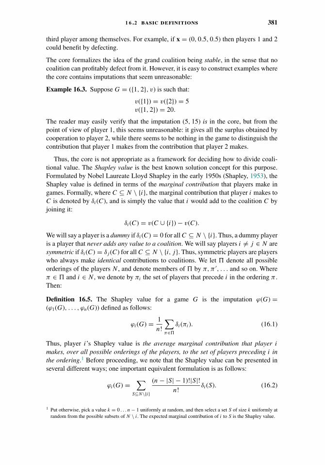
1 6 .2 basic definitions 381
third player among themselves. For example, if x = (0, 0.5, 0.5) then players 1 and 2could benefit by defecting.
The core formalizes the idea of the grand coalition being stable, in the sense that nocoalition can profitably defect from it. However, it is easy to construct examples wherethe core contains imputations that seem unreasonable:
Example 16.3. Suppose G = ({1, 2}, v) is such that:
v({1}) = v({2}) = 5v({1, 2}) = 20.
The reader may easily verify that the imputation (5, 15) is in the core, but from thepoint of view of player 1, this seems unreasonable: it gives all the surplus obtained bycooperation to player 2, while there seems to be nothing in the game to distinguish thecontribution that player 1 makes from the contribution that player 2 makes.
Thus, the core is not appropriate as a framework for deciding how to divide coali-tional value. The Shapley value is the best known solution concept for this purpose.Formulated by Nobel Laureate Lloyd Shapley in the early 1950s (Shapley, 1953), theShapley value is defined in terms of the marginal contribution that players make ingames. Formally, where C ⊆ N \ {i}, the marginal contribution that player i makes toC is denoted by δi(C), and is simply the value that i would add to the coalition C byjoining it:
δi(C) = v(C ∪ {i}) − v(C).
We will say a player is a dummy if δi(C) = 0 for all C ⊆ N \ {i}. Thus, a dummy playeris a player that never adds any value to a coalition. We will say players i �= j ∈ N aresymmetric if δi(C) = δj (C) for all C ⊆ N \ {i, j}. Thus, symmetric players are playerswho always make identical contributions to coalitions. We let � denote all possibleorderings of the players N , and denote members of � by π, π ′, . . . and so on. Whereπ ∈ � and i ∈ N , we denote by πi the set of players that precede i in the ordering π .Then:
Definition 16.5. The Shapley value for a game G is the imputation ϕ(G) =(ϕ1(G), . . . , ϕn(G)) defined as follows:
ϕi(G) = 1
n!
∑π∈�
δi(πi). (16.1)
Thus, player i’s Shapley value is the average marginal contribution that player i
makes, over all possible orderings of the players, to the set of players preceding i inthe ordering.1 Before proceeding, we note that the Shapley value can be presented inseveral different ways; one important equivalent formulation is as follows:
ϕi(G) =∑
S⊆N\{i}
(n − |S| − 1)!|S|!n!
δi(S). (16.2)
1 Put otherwise, pick a value k = 0 . . . n − 1 uniformly at random, and then select a set S of size k uniformly atrandom from the possible subsets of N \ i. The expected marginal contribution of i to S is the Shapley value.
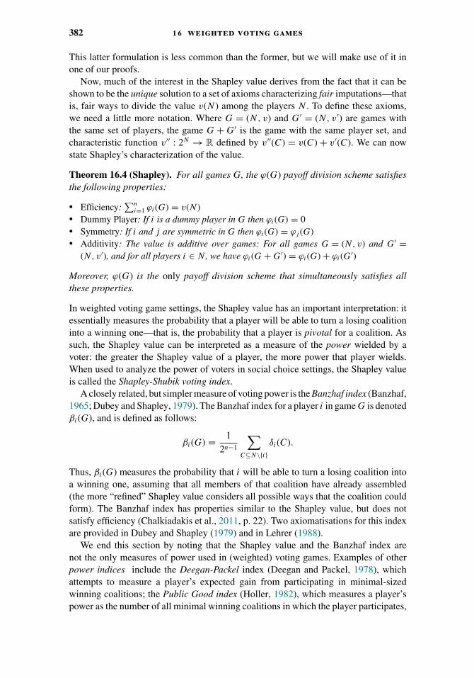
382 1 6 weighted voting games
This latter formulation is less common than the former, but we will make use of it inone of our proofs.
Now, much of the interest in the Shapley value derives from the fact that it can beshown to be the unique solution to a set of axioms characterizing fair imputations—thatis, fair ways to divide the value v(N) among the players N . To define these axioms,we need a little more notation. Where G = (N, v) and G′ = (N, v′) are games withthe same set of players, the game G + G′ is the game with the same player set, andcharacteristic function v′′ : 2N → R defined by v′′(C) = v(C) + v′(C). We can nowstate Shapley’s characterization of the value.
Theorem 16.4 (Shapley). For all games G, the ϕ(G) payoff division scheme satisfiesthe following properties:
� Efficiency:∑n
i=1 ϕi(G) = v(N )� Dummy Player: If i is a dummy player in G then ϕi(G) = 0� Symmetry: If i and j are symmetric in G then ϕi(G) = ϕj (G)� Additivity: The value is additive over games: For all games G = (N, v) and G′ =
(N, v′), and for all players i ∈ N , we have ϕi(G + G′) = ϕi(G) + ϕi(G′)
Moreover, ϕ(G) is the only payoff division scheme that simultaneously satisfies allthese properties.
In weighted voting game settings, the Shapley value has an important interpretation: itessentially measures the probability that a player will be able to turn a losing coalitioninto a winning one—that is, the probability that a player is pivotal for a coalition. Assuch, the Shapley value can be interpreted as a measure of the power wielded by avoter: the greater the Shapley value of a player, the more power that player wields.When used to analyze the power of voters in social choice settings, the Shapley valueis called the Shapley-Shubik voting index.
A closely related, but simpler measure of voting power is the Banzhaf index (Banzhaf,1965; Dubey and Shapley, 1979). The Banzhaf index for a player i in game G is denotedβi(G), and is defined as follows:
βi(G) = 1
2n−1
∑C⊆N\{i}
δi(C).
Thus, βi(G) measures the probability that i will be able to turn a losing coalition intoa winning one, assuming that all members of that coalition have already assembled(the more “refined” Shapley value considers all possible ways that the coalition couldform). The Banzhaf index has properties similar to the Shapley value, but does notsatisfy efficiency (Chalkiadakis et al., 2011, p. 22). Two axiomatisations for this indexare provided in Dubey and Shapley (1979) and in Lehrer (1988).
We end this section by noting that the Shapley value and the Banzhaf index arenot the only measures of power used in (weighted) voting games. Examples of otherpower indices include the Deegan-Packel index (Deegan and Packel, 1978), whichattempts to measure a player’s expected gain from participating in minimal-sizedwinning coalitions; the Public Good index (Holler, 1982), which measures a player’spower as the number of all minimal winning coalitions in which the player participates,

1 6 .3 basic computational properties 383
divided by the sum of all such numbers over all players; and the Coleman initiativeand preventive power indices (Coleman, 1971), which, respectively, correspond to thefraction of losing coalitions that a given player can turn into winning, and vice versa.
16.3 Basic Computational Properties
In this section, we consider computational questions associated with weighted votinggames. The main questions relate to the solution concepts for cooperative games—the core and the Shapley value—that we discussed earlier. However, we will start byconsidering some simpler properties. First, consider the following definition:
Definition 16.6. Let G = (N, v) be a cooperative game, and let i be a player in G.Then i is said to be a veto player in G if v(C) = 0 for all C ⊆ N \ {i}.Thus, a veto player is one whose presence is necessary for a coalition to be winning.The obvious decision problem associated with veto players is as follows:
Name: Veto Player.Instance: Weighted voting game G = [N ; w; q], player i ∈ N .Question: Is i a veto player in G?
We start our survey of computational problems with some good news:
Lemma 16.5. The Veto Player problem is polynomial time solvable for weightedvoting games.
Proof. Given a player i, it suffices check whether the coalition N \ {i} is losing, whichis simple arithmetic.
The significance of this result is made apparent by the following:
Theorem 16.6. A simple cooperative game G = (N, v) has a nonempty core iff ithas a veto player. It follows that it is possible to check in polynomial time whether aweighted voting game has a nonempty core.
Proof. For the left-to-right implication of the first statement, suppose for sake ofcontradiction that G has a nonempty core but no veto player. Take an imputation x inthe core. Because x(N) = 1, we have xi > 0 for some i ∈ N , and hence x(N \ {i}) =1 − xi < 1. However, because i is not a veto player then v(N \ {i}) = 1 > x(N \{i}); contradiction. Now for the right-to-left implication. Suppose i is a veto player,and consider the imputation in which xj = 0 for all j �= i. This imputation is in thecore: because i is a veto player, any deviating coalition would have value 0, and sono such coalition could profitably deviate. The second statement then follows fromLemma 16.5.
Now consider the following problem.
Name: Dummy Player.Instance: Weighted voting game G = [N ; w; q], player i ∈ N .Question: Is i a dummy player in G?
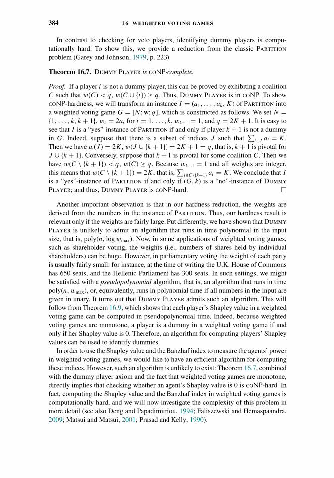
384 1 6 weighted voting games
In contrast to checking for veto players, identifying dummy players is compu-tationally hard. To show this, we provide a reduction from the classic Partitionproblem (Garey and Johnson, 1979, p. 223).
Theorem 16.7. Dummy Player is coNP-complete.
Proof. If a player i is not a dummy player, this can be proved by exhibiting a coalitionC such that w(C) < q, w(C ∪ {i}) ≥ q. Thus, Dummy Player is in coNP. To showcoNP-hardness, we will transform an instance I = (a1, . . . , ak, K) of Partition intoa weighted voting game G = [N ; w; q], which is constructed as follows. We set N ={1, . . . , k, k + 1}, wi = 2ai for i = 1, . . . , k, wk+1 = 1, and q = 2K + 1. It is easy tosee that I is a “yes”-instance of Partition if and only if player k + 1 is not a dummyin G. Indeed, suppose that there is a subset of indices J such that
∑i∈J ai = K .
Then we have w(J ) = 2K , w(J ∪ {k + 1}) = 2K + 1 = q, that is, k + 1 is pivotal forJ ∪ {k + 1}. Conversely, suppose that k + 1 is pivotal for some coalition C. Then wehave w(C \ {k + 1}) < q, w(C) ≥ q. Because wk+1 = 1 and all weights are integer,this means that w(C \ {k + 1}) = 2K , that is,
∑i∈C\{k+1} ai = K . We conclude that I
is a “yes”-instance of Partition if and only if (G, k) is a “no”-instance of DummyPlayer; and thus, Dummy Player is coNP-hard.
Another important observation is that in our hardness reduction, the weights arederived from the numbers in the instance of Partition. Thus, our hardness result isrelevant only if the weights are fairly large. Put differently, we have shown that DummyPlayer is unlikely to admit an algorithm that runs in time polynomial in the inputsize, that is, poly(n, log wmax). Now, in some applications of weighted voting games,such as shareholder voting, the weights (i.e., numbers of shares held by individualshareholders) can be huge. However, in parliamentary voting the weight of each partyis usually fairly small: for instance, at the time of writing the U.K. House of Commonshas 650 seats, and the Hellenic Parliament has 300 seats. In such settings, we mightbe satisfied with a pseudopolynomial algorithm, that is, an algorithm that runs in timepoly(n, wmax), or, equivalently, runs in polynomial time if all numbers in the input aregiven in unary. It turns out that Dummy Player admits such an algorithm. This willfollow from Theorem 16.9, which shows that each player’s Shapley value in a weightedvoting game can be computed in pseudopolynomial time. Indeed, because weightedvoting games are monotone, a player is a dummy in a weighted voting game if andonly if her Shapley value is 0. Therefore, an algorithm for computing players’ Shapleyvalues can be used to identify dummies.
In order to use the Shapley value and the Banzhaf index to measure the agents’ powerin weighted voting games, we would like to have an efficient algorithm for computingthese indices. However, such an algorithm is unlikely to exist: Theorem 16.7, combinedwith the dummy player axiom and the fact that weighted voting games are monotone,directly implies that checking whether an agent’s Shapley value is 0 is coNP-hard. Infact, computing the Shapley value and the Banzhaf index in weighted voting games iscomputationally hard, and we will now investigate the complexity of this problem inmore detail (see also Deng and Papadimitriou, 1994; Faliszewski and Hemaspaandra,2009; Matsui and Matsui, 2001; Prasad and Kelly, 1990).

1 6 .3 basic computational properties 385
To understand just how hard the problem is, we need to recall some concepts fromcomputational complexity that are not quite as well known as notions such as NP-hardness. We want to know how hard it is to compute the Shapley value in a weightedvoting game. Such a problem is not a decision problem like Dummy Player, becausethe output of the problem is not “yes” or “no”: we want a numeric answer. In fact, it isa counting problem. To understand what we mean by a counting problem, consider thefollowing problem: We are given a propositional logic formula ψ , and we are askedhow many satisfying assignments the formula has. This problem is known as #Sat.Notice that the output of #Sat is not “yes” or “no”: it is a natural number. Also noticethat #Sat can be seen to trivially subsume the canonical NP-complete problem Sat,because if we can count the number of satisfying assignments a formula has, we cancertainly tell whether it has at least one (which is what the Sat problem asks). Therelevant complexity class through which to understand the complexity of problemslike #Sat is called #P (Papadimitriou, 1994, p. 442). A problem is in #P if there is anondeterministic polynomial time Turing machine T such that the number of acceptingcomputations of T on a given input x gives the answer to the problem. For the case of#Sat, for example, such a Turing machine simply guesses a valuation for the probleminstance ψ , accepts if that valuation satisfies ψ , and rejects otherwise; clearly, thenumber of accepting runs is exactly the number of satisfying assignments. Hardnesscan be shown in the usual way for computational complexity classes, for example byshowing how we can reduce #Sat. We will now show that computing the Shapleyvalue in weighted voting games is #P-complete.
Theorem 16.8 (Deng and Papadimitriou, 1994). The problem of computing theShapley value of a player i in a given weighted voting game G is #P-complete.
Proof. For membership, consider a Turing machine such that the computations of themachine each correspond to an ordering π of the players; a computation accepts ifδi(πi) = 1. Clearly, the number of accepting computations is n!ϕi(G).
For hardness, we reduce the counting version of the well-known Knapsack problem.In this problem, we are given positive integers a1, . . . , am and a further positive integerK , and we are asked to compute the number of subsets S of {1, . . . , m} such that∑
i∈S ai = K . Computing the number of such sets is known to be #P-hard. In fact,we work with a simplified version of this problem, which is also known to be #P-hard (Papadimitriou, 1994). In this version it is first assumed that K = M
2 , whereM = ∑m
i=1 ai , and further, that all solutions have equal cardinality.We create a weighted voting game with n = m + 1 players, as follows. For players
1 � i � m we set wi = ai , and we set wn = 1. The quota is set to be q =∑
i∈N wi
2 .Now, it is easy to see that for all S ⊆ N , we have v(S) − v(S \ {n}) = 1 iff the
following conditions hold:
1. n ∈ S
2.∑
j∈S wj > (M + 1)/23.∑
j∈S\{n} wj < (M + 1)/2
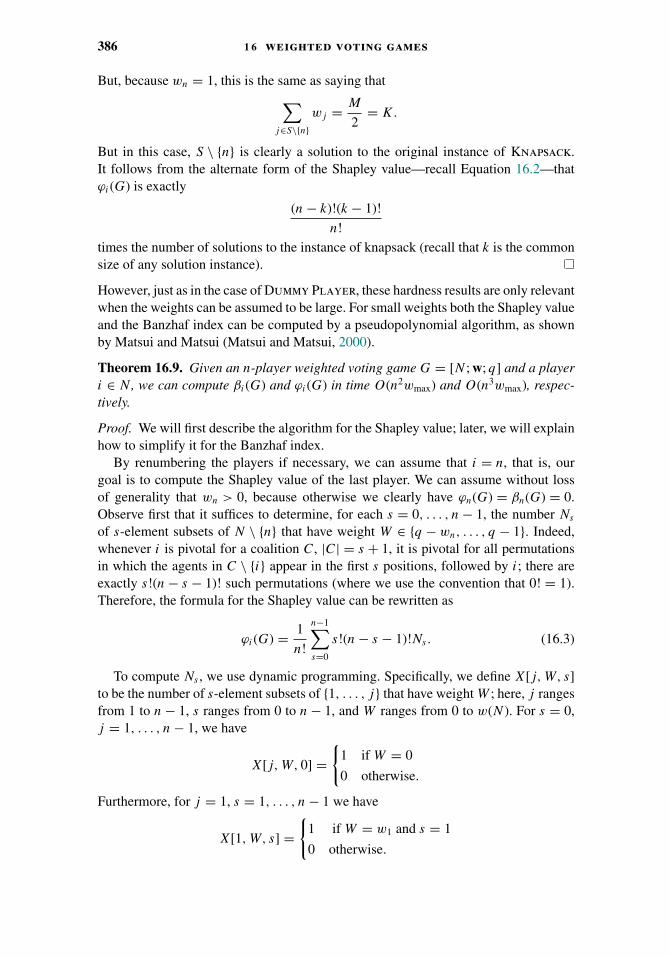
386 1 6 weighted voting games
But, because wn = 1, this is the same as saying that∑j∈S\{n}
wj = M
2= K.
But in this case, S \ {n} is clearly a solution to the original instance of Knapsack.It follows from the alternate form of the Shapley value—recall Equation 16.2—thatϕi(G) is exactly
(n − k)!(k − 1)!
n!times the number of solutions to the instance of knapsack (recall that k is the commonsize of any solution instance).
However, just as in the case of Dummy Player, these hardness results are only relevantwhen the weights can be assumed to be large. For small weights both the Shapley valueand the Banzhaf index can be computed by a pseudopolynomial algorithm, as shownby Matsui and Matsui (Matsui and Matsui, 2000).
Theorem 16.9. Given an n-player weighted voting game G = [N ; w; q] and a playeri ∈ N , we can compute βi(G) and ϕi(G) in time O(n2wmax) and O(n3wmax), respec-tively.
Proof. We will first describe the algorithm for the Shapley value; later, we will explainhow to simplify it for the Banzhaf index.
By renumbering the players if necessary, we can assume that i = n, that is, ourgoal is to compute the Shapley value of the last player. We can assume without lossof generality that wn > 0, because otherwise we clearly have ϕn(G) = βn(G) = 0.Observe first that it suffices to determine, for each s = 0, . . . , n − 1, the number Ns
of s-element subsets of N \ {n} that have weight W ∈ {q − wn, . . . , q − 1}. Indeed,whenever i is pivotal for a coalition C, |C| = s + 1, it is pivotal for all permutationsin which the agents in C \ {i} appear in the first s positions, followed by i; there areexactly s!(n − s − 1)! such permutations (where we use the convention that 0! = 1).Therefore, the formula for the Shapley value can be rewritten as
ϕi(G) = 1
n!
n−1∑s=0
s!(n − s − 1)!Ns. (16.3)
To compute Ns , we use dynamic programming. Specifically, we define X[j, W, s]to be the number of s-element subsets of {1, . . . , j} that have weight W ; here, j rangesfrom 1 to n − 1, s ranges from 0 to n − 1, and W ranges from 0 to w(N). For s = 0,j = 1, . . . , n − 1, we have
X[j, W, 0] ={
1 if W = 0
0 otherwise.
Furthermore, for j = 1, s = 1, . . . , n − 1 we have
X[1, W, s] ={
1 if W = w1 and s = 1
0 otherwise.
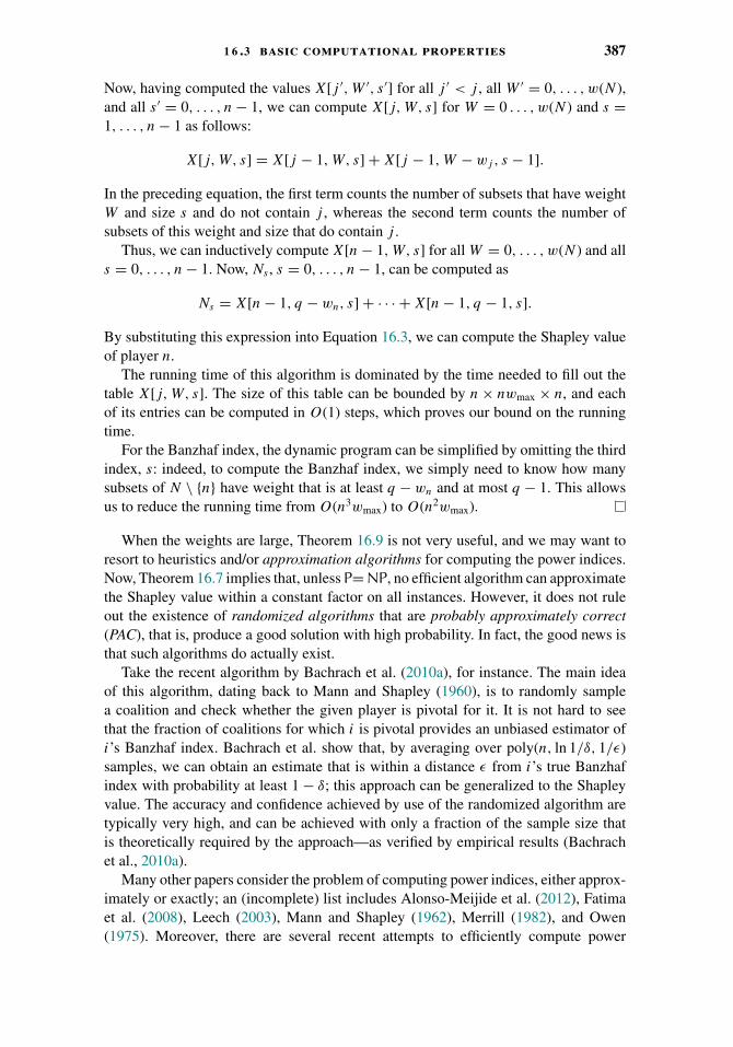
1 6 .3 basic computational properties 387
Now, having computed the values X[j ′, W ′, s ′] for all j ′ < j , all W ′ = 0, . . . , w(N),and all s ′ = 0, . . . , n − 1, we can compute X[j, W, s] for W = 0 . . . , w(N) and s =1, . . . , n − 1 as follows:
X[j, W, s] = X[j − 1, W, s] + X[j − 1, W − wj, s − 1].
In the preceding equation, the first term counts the number of subsets that have weightW and size s and do not contain j , whereas the second term counts the number ofsubsets of this weight and size that do contain j .
Thus, we can inductively compute X[n − 1, W, s] for all W = 0, . . . , w(N) and alls = 0, . . . , n − 1. Now, Ns , s = 0, . . . , n − 1, can be computed as
Ns = X[n − 1, q − wn, s] + · · · + X[n − 1, q − 1, s].
By substituting this expression into Equation 16.3, we can compute the Shapley valueof player n.
The running time of this algorithm is dominated by the time needed to fill out thetable X[j, W, s]. The size of this table can be bounded by n × nwmax × n, and eachof its entries can be computed in O(1) steps, which proves our bound on the runningtime.
For the Banzhaf index, the dynamic program can be simplified by omitting the thirdindex, s: indeed, to compute the Banzhaf index, we simply need to know how manysubsets of N \ {n} have weight that is at least q − wn and at most q − 1. This allowsus to reduce the running time from O(n3wmax) to O(n2wmax).
When the weights are large, Theorem 16.9 is not very useful, and we may want toresort to heuristics and/or approximation algorithms for computing the power indices.Now, Theorem 16.7 implies that, unless P=NP, no efficient algorithm can approximatethe Shapley value within a constant factor on all instances. However, it does not ruleout the existence of randomized algorithms that are probably approximately correct(PAC), that is, produce a good solution with high probability. In fact, the good news isthat such algorithms do actually exist.
Take the recent algorithm by Bachrach et al. (2010a), for instance. The main ideaof this algorithm, dating back to Mann and Shapley (1960), is to randomly samplea coalition and check whether the given player is pivotal for it. It is not hard to seethat the fraction of coalitions for which i is pivotal provides an unbiased estimator ofi’s Banzhaf index. Bachrach et al. show that, by averaging over poly(n, ln 1/δ, 1/ε)samples, we can obtain an estimate that is within a distance ε from i’s true Banzhafindex with probability at least 1 − δ; this approach can be generalized to the Shapleyvalue. The accuracy and confidence achieved by use of the randomized algorithm aretypically very high, and can be achieved with only a fraction of the sample size thatis theoretically required by the approach—as verified by empirical results (Bachrachet al., 2010a).
Many other papers consider the problem of computing power indices, either approx-imately or exactly; an (incomplete) list includes Alonso-Meijide et al. (2012), Fatimaet al. (2008), Leech (2003), Mann and Shapley (1962), Merrill (1982), and Owen(1975). Moreover, there are several recent attempts to efficiently compute power

388 1 6 weighted voting games
indices in restricted settings, taking advantage of specific domain characteristics (see,e.g., Duran et al., 2003; Bachrach and Shah, 2013; See et al., 2014).
16.4 Voter Weight versus Voter Power
In weighted voting games, one might expect that there is a close correlation betweenthe weight wi that a player i is assigned, and the power that player i wields. Afterall, a player’s ability to turn a losing coalition into a winning coalition derives fromtheir weight. This intuition is not entirely incorrect: it is not hard to show that poweris monotone in weight—that is, for any weighted voting game G = [N ; w; q] andany two players i, j ∈ N we have ϕi(G) ≤ ϕj (G) if and only if wi ≤ wj . However,the power of an agent cannot be simply represented by its weight, in general: in thatsense,“weighted voting doesn’t work” (Banzhaf, 1965). Indeed, two agents may haveidentical voting power even if their weights differ dramatically.
Example 16.10. After the May 2010 elections in the United Kingdom, the ConservativeParty had 307 seats, the Labour Party had 258 seats, the Liberal Democrats (LibDems)had 57 seats, and all other parties shared the remaining 28 seats (with the most powerfulof them getting 8 seats). The U.K. Parliament is a simple majority system, so the quotais 326. To keep things simple in this analysis, we will treat the “other” parties as asingle block (the other parties would be unlikely to act as a block in practice).
Now, it is easy to see that in this weighted voting game there are two two-partycoalitions (Conservatives+Labour and Conservatives+LibDems) that can get a majorityof seats. Moreover, if Labour or LibDems want to form a coalition that does not includeConservatives, they need each other and the others. Thus, Labour and LibDems have thesame Shapley value, despite being vastly different in size. In more detail, the Shapleyvalues are as follows:
i ϕi
Conservative 1/2Labour 1/6LibDem 1/6Other 1/6
The phenomenon illustrated in Example 16.10 has been observed in many decision-making bodies. It explains why major parties often end up making concessions tosmaller parties in order to form a winning coalition: the small parties may wieldsubstantial voting power. Example 16.10 also indicates that to determine an agent’spower, we have to take into account the distribution of the other players’ weights aswell as the quota. In particular, if we keep the weights fixed, but alter the quota, anagent’s power can change considerably.
Example 16.11. Consider a weighted voting game with two players of weight 4 andtwo players of weight 1. If the quota is set to 10, the only winning coalition is the grandcoalition, so each player’s Shapley value is 1/4. If the quota is set to 8, the smaller
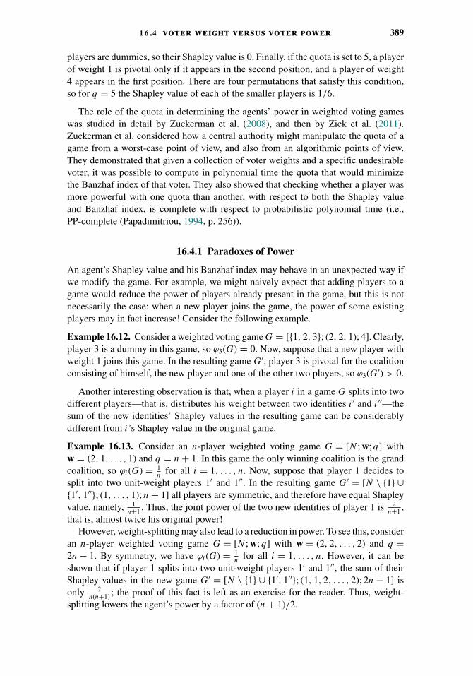
1 6 .4 voter weight versus voter power 389
players are dummies, so their Shapley value is 0. Finally, if the quota is set to 5, a playerof weight 1 is pivotal only if it appears in the second position, and a player of weight4 appears in the first position. There are four permutations that satisfy this condition,so for q = 5 the Shapley value of each of the smaller players is 1/6.
The role of the quota in determining the agents’ power in weighted voting gameswas studied in detail by Zuckerman et al. (2008), and then by Zick et al. (2011).Zuckerman et al. considered how a central authority might manipulate the quota of agame from a worst-case point of view, and also from an algorithmic points of view.They demonstrated that given a collection of voter weights and a specific undesirablevoter, it was possible to compute in polynomial time the quota that would minimizethe Banzhaf index of that voter. They also showed that checking whether a player wasmore powerful with one quota than another, with respect to both the Shapley valueand Banzhaf index, is complete with respect to probabilistic polynomial time (i.e.,PP-complete (Papadimitriou, 1994, p. 256)).
16.4.1 Paradoxes of Power
An agent’s Shapley value and his Banzhaf index may behave in an unexpected way ifwe modify the game. For example, we might naively expect that adding players to agame would reduce the power of players already present in the game, but this is notnecessarily the case: when a new player joins the game, the power of some existingplayers may in fact increase! Consider the following example.
Example 16.12. Consider a weighted voting game G = [{1, 2, 3}; (2, 2, 1); 4]. Clearly,player 3 is a dummy in this game, so ϕ3(G) = 0. Now, suppose that a new player withweight 1 joins this game. In the resulting game G′, player 3 is pivotal for the coalitionconsisting of himself, the new player and one of the other two players, so ϕ3(G′) > 0.
Another interesting observation is that, when a player i in a game G splits into twodifferent players—that is, distributes his weight between two identities i ′ and i ′′—thesum of the new identities’ Shapley values in the resulting game can be considerablydifferent from i’s Shapley value in the original game.
Example 16.13. Consider an n-player weighted voting game G = [N ; w; q] withw = (2, 1, . . . , 1) and q = n + 1. In this game the only winning coalition is the grandcoalition, so ϕi(G) = 1
nfor all i = 1, . . . , n. Now, suppose that player 1 decides to
split into two unit-weight players 1′ and 1′′. In the resulting game G′ = [N \ {1} ∪{1′, 1′′}; (1, . . . , 1); n + 1] all players are symmetric, and therefore have equal Shapleyvalue, namely, 1
n+1 . Thus, the joint power of the two new identities of player 1 is 2n+1 ,
that is, almost twice his original power!However, weight-splitting may also lead to a reduction in power. To see this, consider
an n-player weighted voting game G = [N ; w; q] with w = (2, 2, . . . , 2) and q =2n − 1. By symmetry, we have ϕi(G) = 1
nfor all i = 1, . . . , n. However, it can be
shown that if player 1 splits into two unit-weight players 1′ and 1′′, the sum of theirShapley values in the new game G′ = [N \ {1} ∪ {1′, 1′′}; (1, 1, 2, . . . , 2); 2n − 1] isonly 2
n(n+1) ; the proof of this fact is left as an exercise for the reader. Thus, weight-splitting lowers the agent’s power by a factor of (n + 1)/2.

390 1 6 weighted voting games
The phenomena illustrated in Examples 16.12 and 16.13 are known as the paradoxof new members and the paradox of size, respectively. There are several other forms ofcounterintuitive behavior exhibited by the power indices; jointly, they are referred to asthe paradoxes of power. These paradoxes are discussed by Felsenthal and Machover(1998) and subsequently by Laruelle and Valenciano (2005) (see also the referencestherein). The paradox of size is studied in detail by Aziz et al. (2011), who showthat the games described in Example 16.13 exhibit the strongest form of this paradoxpossible: in an n-player weighted voting game, splitting into two identities can increase(respectively, decrease) an agent’s Shapley value by at most a factor of 2n/(n + 1)(respectively, (n + 1)/2). Aziz et al. (2011) also show that deciding whether a givenplayer can split so as to increase his power is NP-hard. Rey and Rothe (2014) showsimilar hardness results for coalitional splitting, merging and annexation in weightedvoting games.
16.5 Simple Games and Yes/No Voting Systems
At this point, let us step back from considering weighted voting games specifically,and consider the wider class of social choice systems of which weighted voting gamesare an instance. Yes/No voting systems are voting systems in which a proposal (e.g.,a new law, or a change to tax regulations) is pitted against the status quo (Taylor andZwicker, 1999). Decision making in many political bodies can be understood as ayes/no voting system (e.g., in the United Kingdom, the voting system of the Houseof Commons; in the European Union, the voting system in the enlarged EU; in theUnited States, the U.S. federal system; in the United Nations, the voting system ofthe Security Council (Taylor, 1995)). Formally, yes/no voting systems have a verysimple structure:
Definition 16.7. A yes/no voting system is a pair Y = (N, W ), where N = {1, . . . , n}is the set of voters, and W ⊆ 2N is the set of winning coalitions, with the intendedinterpretation that, if C ∈ W , then C would be able to determine the outcome (either“yes” or “no”) to the question at hand, should they collectively choose to.
Notice that yes/no voting systems can alternatively be understood as simple coopera-tive games. Formally, we can understand a simple game G = (N, v : 2N → {0, 1}) asdefining a yes/no voting system YG = (N, WG) in which
WG = {C ⊆ N | v(C) = 1}.
Results relating to simple games can thus be applied directly to yes/no voting sys-tems, and we can therefore choose to work with whichever model we find mostconvenient.
Several possible conditions on yes/no voting games suggest themselves as beingappropriate for some (though of course not all) scenarios:
� Nontriviality: There are some winning coalitions, but not all coalitions are winning—formally, ∅ ⊂ W ⊂ 2N .
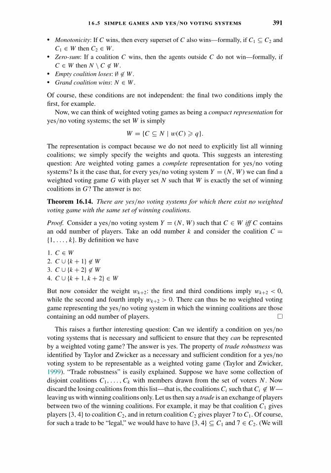
1 6 .5 simple games and yes/no voting systems 391
� Monotonicity: If C wins, then every superset of C also wins—formally, if C1 ⊆ C2 andC1 ∈ W then C2 ∈ W .
� Zero-sum: If a coalition C wins, then the agents outside C do not win—formally, ifC ∈ W then N \ C �∈ W .
� Empty coalition loses: ∅ �∈ W .� Grand coalition wins: N ∈ W .
Of course, these conditions are not independent: the final two conditions imply thefirst, for example.
Now, we can think of weighted voting games as being a compact representation foryes/no voting systems; the set W is simply
W = {C ⊆ N | w(C) � q}.The representation is compact because we do not need to explicitly list all winningcoalitions; we simply specify the weights and quota. This suggests an interestingquestion: Are weighted voting games a complete representation for yes/no votingsystems? Is it the case that, for every yes/no voting system Y = (N, W ) we can find aweighted voting game G with player set N such that W is exactly the set of winningcoalitions in G? The answer is no:
Theorem 16.14. There are yes/no voting systems for which there exist no weightedvoting game with the same set of winning coalitions.
Proof. Consider a yes/no voting system Y = (N, W ) such that C ∈ W iff C containsan odd number of players. Take an odd number k and consider the coalition C ={1, . . . , k}. By definition we have
1. C ∈ W
2. C ∪ {k + 1} �∈ W
3. C ∪ {k + 2} �∈ W
4. C ∪ {k + 1, k + 2} ∈ W
But now consider the weight wk+2: the first and third conditions imply wk+2 < 0,while the second and fourth imply wk+2 > 0. There can thus be no weighted votinggame representing the yes/no voting system in which the winning coalitions are thosecontaining an odd number of players.
This raises a further interesting question: Can we identify a condition on yes/novoting systems that is necessary and sufficient to ensure that they can be representedby a weighted voting game? The answer is yes. The property of trade robustness wasidentified by Taylor and Zwicker as a necessary and sufficient condition for a yes/novoting system to be representable as a weighted voting game (Taylor and Zwicker,1999). “Trade robustness” is easily explained. Suppose we have some collection ofdisjoint coalitions C1, . . . , Ck with members drawn from the set of voters N . Nowdiscard the losing coalitions from this list—that is, the coalitions Ci such that Ci �∈ W—leaving us with winning coalitions only. Let us then say a trade is an exchange of playersbetween two of the winning coalitions. For example, it may be that coalition C1 givesplayers {3, 4} to coalition C2, and in return coalition C2 gives player 7 to C1. Of course,for such a trade to be “legal,” we would have to have {3, 4} ⊆ C1 and 7 ∈ C2. (We will
392 1 6 weighted voting games
permit the possibility of empty sets of players being transferred in a trade.) Then wehave:
Definition 16.8. A yes/no voting game is said to be trade robust if, after an any legalsequence of trades starting with a set of winning coalitions, at least one of the resultingcoalitions is still winning.
We have:
Theorem 16.15 (Taylor and Zwicker, 1999). For every yes/no voting system Y =(N, W ), there exists a weighted voting game that is equivalent to Y iff Y is trade robust.
To further illustrate trade robustness, let us consider a richer example.
Example 16.16. Consider a game G = (N, v) with N = {1, 2, 3, 4} given by
v(C) = 0, if |C| ≤ 1
v(C) = 1, if |C| ≥ 3
v({1, 2}) = v({3, 4}) = v({1, 4}) = v({2, 3}) = 1,
v({1, 3}) = v({2, 4}) = 0.
This game is not trade robust, because when two winning coalitions C1 = {1, 2} andC2 = {3, 4} trade members (2 moves from C1 to C2 and 3 moves from C2 to C1), bothof the resulting coalitions are losing.
Notice, however, G can be represented as an intersection of two weighted votinggames, in the following sense. Let w1 = (1, 0, 1, 0), w2 = (0, 1, 0, 1), q1 = q2 = 1,and set G1 = [N ; w1; q1], G2 = [N ; w2; q2]. Observe that a coalition C is winningin both G1 and G2 if and only if it contains both an even-numbered player and anodd-numbered player—that is, if and only if v(C) = 1.
The construction presented in Example 16.16 can be used to describe other simplegames in the language of weighted voting games. That is, we can take k ≥ 1 weightedvoting games G1, . . . , Gk over the same set of players N , and define a new simplegame G = (N, v) by setting v(C) = 1 if and only if C is a winning coalition in each ofthe underlying games G1, . . . , Gk . It turns out that any yes/no game can be obtainedin this manner.
Theorem 16.17. For any simple game G = (N, v), there exists a list of weightedvoting games G1, . . . , Gk , where Gj = [N ; wj ; qj ] for j = 1, . . . , k such that for anycoalition C ⊆ N it holds that v(C) = 1 if and only if wj (C) ≥ qj for each j = 1, . . . , k.
Proof. Let C1, . . . , Ck be the list of losing coalitions in G. We define the j th weightedvoting game Gj by setting w
ji = 0 if i ∈ Cj and w
ji = 1 if i �∈ Cj (here w
ji denotes
the weight of the ith player in Gj ) and qj = 1. That is, a coalition C is winning inGj if and only if it contains an agent i �∈ Cj , or, equivalently, if and only if it is not asubset of Cj .
Consider a coalition C with v(C) = 1. By monotonicity, C is not a subset of anylosing coalition, so we have wj (C) ≥ qj for any j = 1, . . . , k. On the other hand, if
1 6 .5 simple games and yes/no voting systems 393
v(C) = 0, then C = Cj for some j = 1, . . . , k, so wj (C) = 0 < qj . Thus, the theoremis proved.
Games that are represented as intersections of k weighted voting games areknown as k-weighted voting games or vector weighted voting games. More for-mally, a k-weighted voting game is given by a set of players N , |N | = n, foreach player i ∈ N , a k-dimensional weight vector wi = (w1
i , . . . , wki ) whose entries
are nonnegative integers, and k nonnegative integer quotas q1, . . . , qk; we writeG = [N ; w1, . . . , wn; q1, . . . , qk]. A coalition C ⊆ N is deemed to be winning inG if and only if
∑i∈C w
ji ≥ qj for all j = 1, . . . , k.
Observe that G can be associated with k weighted voting games G1, . . . , Gk , whereGj = [N ; (wj
1 , . . . , wjn); qj ]; these games are called the component games of G, and
the weight vector of the j th game is denoted by wj . Clearly, any vector voting game isa simple game, and Theorem 16.17 shows that the converse is also true.
It is important to note that vector weighted voting games are not theoretical con-structs: they feature quite prominently in our lives. For example, the following politicalsystems can be understood as vector weighted voting games (Bilbao et al., 2002; Taylor,1995; Taylor and Zwicker, 1999):
� The U.S. federal system is a 2-weighted voting game, in which the components corre-spond to the two chambers (the House of Representatives and the Senate). The playersare the president, vice president, senators, and representatives. In the game correspond-ing to the House of Representatives, senators have zero weight, while in the gamecorresponding to the Senate, representatives have zero weight. The president is the onlyplayer to have nonzero weight in both games.
� The voting system of the European Union is a 3-weighted voting game (Bilbao et al.,2002). Specifically, in the Council of the European Union, a law requires the supportof 50% of the countries, 62% of the population of the European Union, and 74% of the“commissioners” of the EU. Each member state is a player, so (as of 2011) the playersare as follows:
Germany, United Kingdom, France, Italy, Spain, Poland, Romania, The Netherlands, Greece,Czech Republic, Belgium, Hungary, Portugal, Sweden, Bulgaria, Austria, Slovak Repub-lic, Denmark, Finland, Ireland, Lithuania, Latvia, Slovenia, Estonia, Cyprus, Luxembourg,Malta.
The three component games in the EU voting system are shown in Figure 16.1 (we omitthe player set N = {1, . . . , 27}, as well as all brackets and parentheses, from the nota-tion). Weights in the first game are assigned according to the number of commissionersthe respective member state has. The second game is a simple majority game: everymember state gets one vote, and a law must have the support of at least 14 memberstates. In the third game, weights are assigned in proportion to the population of therespective member state.
Theorem 16.17 allows us to represent any simple game G as a vector weightedvoting game; however, the number k of the component games can be quite large (and,in particular, exponential in the number of players n). The number of the component
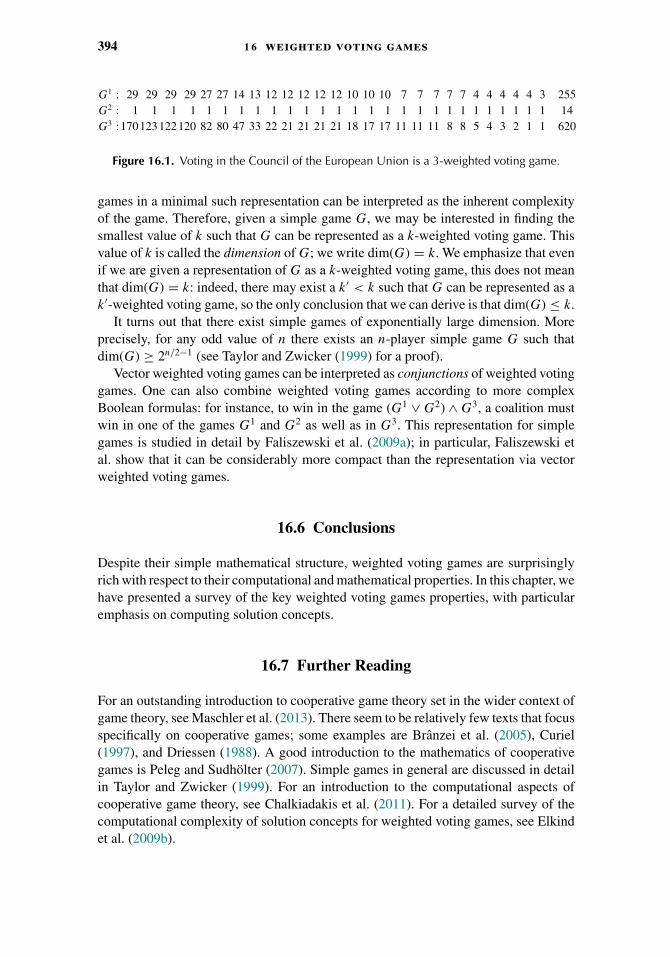
394 1 6 weighted voting games
G1 : 29 29 29 29 27 27 14 13 12 12 12 12 12 10 10 10 7 7 7 7 7 4 4 4 4 4 3G2 : 1 1 1 1 1 1 1 1 1 1 1 1 1 1 1 1 1 1 1 1 1 1 1 1 1 1 1G3 :170123122120 82 80 47 33 22 21 21 21 21 18 17 17 11 11 11 8 8 5 4 3 2 1 1
25514620
Figure 16.1. Voting in the Council of the European Union is a 3-weighted voting game.
games in a minimal such representation can be interpreted as the inherent complexityof the game. Therefore, given a simple game G, we may be interested in finding thesmallest value of k such that G can be represented as a k-weighted voting game. Thisvalue of k is called the dimension of G; we write dim(G) = k. We emphasize that evenif we are given a representation of G as a k-weighted voting game, this does not meanthat dim(G) = k: indeed, there may exist a k′ < k such that G can be represented as ak′-weighted voting game, so the only conclusion that we can derive is that dim(G) ≤ k.
It turns out that there exist simple games of exponentially large dimension. Moreprecisely, for any odd value of n there exists an n-player simple game G such thatdim(G) ≥ 2n/2−1 (see Taylor and Zwicker (1999) for a proof).
Vector weighted voting games can be interpreted as conjunctions of weighted votinggames. One can also combine weighted voting games according to more complexBoolean formulas: for instance, to win in the game (G1 ∨ G2) ∧ G3, a coalition mustwin in one of the games G1 and G2 as well as in G3. This representation for simplegames is studied in detail by Faliszewski et al. (2009a); in particular, Faliszewski etal. show that it can be considerably more compact than the representation via vectorweighted voting games.
16.6 Conclusions
Despite their simple mathematical structure, weighted voting games are surprisinglyrich with respect to their computational and mathematical properties. In this chapter, wehave presented a survey of the key weighted voting games properties, with particularemphasis on computing solution concepts.
16.7 Further Reading
For an outstanding introduction to cooperative game theory set in the wider context ofgame theory, see Maschler et al. (2013). There seem to be relatively few texts that focusspecifically on cooperative games; some examples are Branzei et al. (2005), Curiel(1997), and Driessen (1988). A good introduction to the mathematics of cooperativegames is Peleg and Sudholter (2007). Simple games in general are discussed in detailin Taylor and Zwicker (1999). For an introduction to the computational aspects ofcooperative game theory, see Chalkiadakis et al. (2011). For a detailed survey of thecomputational complexity of solution concepts for weighted voting games, see Elkindet al. (2009b).

acknowledgments 395
Acknowledgments
We would like to thank Edith Elkind for her permission to adapt co-authored materialfor this chapter, and in particular, material from our book (Chalkiadakis et al., 2011).We would also like to thank our editors (in particular Jerome Lang and Ariel Proccacia)and our reviewers, Yair Zick and Yoram Bachrach, for their invaluable corrections andcomments. Wooldridge was supported by the European Research Council under grant291528 (“RACE”).


PART IV
Additional Topics


CHAPTER 17
Judgment Aggregation
Ulle Endriss
17.1 Introduction
Social choice theory deals with the aggregation of information supplied by severalindividuals into a collective decision that appropriately reflects the views of the groupas a whole. The most widely considered type of information is preference information.For example, in an election each voter supplies information regarding her preferencesover the set of candidates and the voting rule in operation aggregates this informationinto the collective decision of which candidate wins the election. But the methodologyof social choice theory may just as well be applied to other types of information, suchas beliefs about whether certain statements are true or false. Judgment aggregation (JAfrom here on), the topic of this chapter, is an elegant formal framework for modelingthis form of aggregation.
Let us begin with a famous example from the work of legal scholars Lewis A. Korn-hauser and Lawrence G. Sager (Kornhauser and Sager, 1993). Suppose three judgestogether have to decide on a case regarding an alleged breach of contract. They willtry to establish whether (a) the document in question really is a binding contract andwhether (b) the promise given in that document really has been breached. Legal doc-trine stipulates that the defendant is liable if and only if there have been both a contractand a breach. The three judges differ in their assessment regarding the two premises(and thus also regarding the conclusion):
Contract? Breach? Liable?
Judge Joe: Yes Yes YesJudge Judy: Yes No NoJudge Jules: No Yes No
What should be their collective decision regarding the defendant’s liability? If theyimplement a majority vote on the conclusion (the rightmost column), then they willfind the defendant not liable (by a 2:1 majority). If instead they vote on the premises,
399
400 1 7 judgment aggregation
they will have to accept that the contract was binding (by a 2:1 majority) and that ithas been breached (again, by a 2:1 majority). In the latter case, legal doctrine requiresthem to find the defendant liable. Thus, in the presence of this doctrine, two seeminglyreasonable procedures lead to contradictory outcomes. This is known as the doctrinalparadox.
Now consider a more abstract rendering of the problem. Three judges have to assessthe truth of three formulas of propositional logic: p (“contract”), q (“breach”), andtheir conjunction p ∧ q (which we said was equivalent to “liable”). This time we alsoinclude the result of applying majority voting to each formula:
p q p ∧ q
Judge 1: Yes Yes YesJudge 2: Yes No NoJudge 3: No Yes No
Majority: Yes Yes No
Thus, we again obtain an unexpected, that is, paradoxical, outcome: despite the fact thateach individual judge provides a logically consistent set of judgments, the majority ruleresults in a judgment set that is inconsistent (there exists no assignment of truth valuesto propositional variables that would make p true, q true, and p ∧ q false). So, ourexample demonstrates not merely a dilemma between premise-driven and conclusion-driven approaches to collective decision making, but rather a dilemma between a certainresponsiveness to the views of decision makers (by respecting their majority decisions)and the consistency of collective decisions. This point was first made by the politicalphilosopher Philip Pettit, who noted that this dilemma is not only relevant to analyticaljurisprudence, but may strike whenever a group of people engage in a democraticdecision making process involving several mutually dependent propositions (Pettit,2001). Pettit introduced the term discursive dilemma for this problem, both to stressits relevance to the political discourse in general and to reflect the fact that we do notactually require the external legal doctrine from the original example to exhibit theproblem.
Is there a way around this dilemma? Maybe the majority rule is the root of theproblem and there are other methods of aggregation that can ensure a consistent out-come? In a seminal paper that introduced a formal framework for JA that permits usto ask and answer such questions, Christian List and Philip Pettit showed that this isnot the case (List and Pettit, 2002): it is impossible to devise an aggregation rule thatavoids the discursive dilemma—at least if we wish to maintain some of the most basicproperties of the majority rule that, arguably, are fundamental features of any reason-able form of aggregation. These properties are anonymity (“treat all judges symmet-rically”), neutrality (“treat all propositions symmetrically”), and independence (“basethe collective decision regarding a given proposition only on the individual judgmentsregarding that same proposition”). We formally state and prove this surprising result inSection 17.2.4.
The work of List and Pettit employs the axiomatic method commonly used ineconomic theory, and specifically in social choice theory, for example, to establish
1 7 .1 introduction 401
impossibility results in preference aggregation. This—together with the fact that JAis a natural framework in which to embed other frameworks of aggregation, specifi-cally preference aggregation (see Section 17.2.2)—has triggered a sustained interestin JA among economic theorists. Their work has led to a deeper understanding of thecircumstances under which it is either possible or impossible to perform consistentaggregation. In particular, these results clarify the role of the agenda, the set of propo-sitions to be judged. For instance, it is easy to see that when the agenda consists solelyof literals (i.e., propositional variables and their negations), then the majority rule willnever produce an inconsistent outcome. We review some representative examples ofsuch results later on in Section 17.4.
Besides analytical jurisprudence, political philosophy, and economic theory, JAis also relevant to computer science, particularly to artificial intelligence (AI). Forinstance, JA suggests itself as a framework in which to study collective decisionmaking in systems of autonomous software agents, given that logic is the preferredlanguage in which to model the beliefs of a single such agent (we will discuss thisand other applications of JA in computer science in Section 17.6). In fact, there areclose connections between some of the work on belief merging in AI and the modelof JA under consideration here (we briefly comment on some of these connections inSection 17.5.1). Once computer scientists got interested in JA, this naturally led to aview of aggregation procedures as algorithms and, more generally, of reasoning aboutquestions in JA as computational problems. We will adopt this perspective also in partsof this chapter and report, for instance, on the computational difficulty of recognizingwhether an agenda is sufficiently simple to avoid all occurrences of the discursivedilemma for a given aggregation procedure.
The remainder of this chapter is organized as follows. Section 17.2 defines the formalframework of JA and, to exemplify the expressive power of the framework, shows howpreference aggregation can be embedded into JA. The same section also introduces themost commonly used axioms in JA and then proves the basic impossibility theorem ofList and Pettit mentioned earlier. Section 17.3 reviews three specific types of aggre-gators in some detail: quota rules, distance-based aggregators, and the premise-basedrule. In the context of quota rules, we also discuss examples of the axiomatic charac-terization of aggregators; we use distance-based aggregation to exemplify the analysisof the complexity of winner determination in JA; and we review questions of strategicmanipulation in the section dedicated to premise-based aggregation. Section 17.4 isdevoted to agenda characterization results that clarify the extent to which instances ofthe discursive dilemma depend on the structural complexity of the agenda on whichjudges are asked to vote. Section 17.5 discusses related frameworks for collective deci-sion making and Section 17.6 sketches possible applications in computer science. Toimprove readability, bibliographic references are kept to a minimum in the body of thechapter; such details are instead supplied in Section 17.7, which also provides pointersto further reading.
Throughout this chapter we shall assume familiarity with the very basics of proposi-tional logic (see, e.g., van Dalen, 2013), particularly the notion of logical consistency.In a few selected places we furthermore assume familiarity with basic concepts fromthe theory of computational complexity (see, e.g., Arora and Barak, 2009, or theintroductory chapter of this volume).
402 1 7 judgment aggregation
17.2 Basics
In this section we define the formal framework of JA, which originally was laid down byList and Pettit (2002) and since then has been further refined by several authors, notablyDietrich (2007).1 We also sketch how to embed preference aggregation problems intoJA, review the most important axioms encoding desirable properties of aggregatorsproposed in the literature, and discuss a basic impossibility theorem.
17.2.1 Formal Framework
Let L be a set of propositional formulas built from a finite set of propositional variablesusing the usual connectives ¬, ∧, ∨, →, ↔, and the constants ( (“true”) and ⊥(“false”). For every formula ϕ, define ∼ϕ to be the complement of ϕ, that is, ∼ϕ = ¬ϕ
if ϕ is not negated, and ∼ϕ = ψ if ϕ = ¬ψ for some formula ψ . We write � |= ϕ incase formula ϕ is true whenever all formulas in the set � are true.
An agenda is a finite nonempty subset � ⊆ L that does not contain any doubly-negated formulas and that is closed under complementation (i.e., if ϕ ∈ � then ∼ϕ ∈�).2 For ease of exposition, we shall assume that � is nontrivial in the sense of including(at least) two logically independent formulas α and β (i.e., all of {α, β}, {α,∼β},{∼α, β}, and {∼α,∼β} are consistent).3 Some authors exclude the possibility of �
including a tautology or a contradiction, but we do not make this assumption here. Ajudgment set J for � is a subset J ⊆ �. For example, the discursive dilemma sketchedin the introduction involved the agenda � = {p,¬p, q,¬q, p ∧ q,¬(p ∧ q)}. Thejudgment set of judge 3 was J3 = {¬p, q,¬(p ∧ q)}, that is, rather than labelingformulas ϕ with “yes” and “no,” as we did earlier, we now either include ϕ or ∼ϕ inthe relevant judgment set.
We call a judgment set J complete if ϕ ∈ J or ∼ϕ ∈ J for all ϕ ∈ �; we call itcomplement-free if for no ϕ ∈ � we have both ϕ ∈ J and ∼ϕ ∈ J ; and we call itconsistent if there exists an assignment of truth values (true or false) to propositionalvariables under which all formulas in J are true. Note that every consistent set iscomplement-free, but the converse is not true. For instance, the majority judgment setfrom our introductory example, {p, q,¬(p ∧ q)}, is clearly complete and complement-free, but it is not consistent: if we set both p and q to be true, then the third formula¬(p ∧ q) necessarily comes out as false. Let J (�) denote the set of all complete andconsistent subsets of �.
Let N = {1, . . . , n} be a set of n > 1 judges (or individuals, or agents). For ease ofexposition, we shall assume that n is odd. We often refer to subsets C ⊆ N as coalitionsand we write C := N \ C for the complement of C. A profile is a vector of judgmentsets J = (J1, . . . , Jn) ∈ J (�)n, one for each judge. We write N J
ϕ := {i ∈ N | ϕ ∈ Ji}for the set of judges accepting the formula ϕ in profile J .
1 The particular mode of exposition chosen here is closely based on the author’s joint work with Umberto Grandiand Daniele Porello (Endriss et al., 2012).
2 The reason for introducing the notion of complement is that it often simplifies presentation. For example, ifϕ ∈ �, then the “negation of ϕ” will only be in � if ϕ is not a negated formula, while we can speak of the“complement of ϕ” without having to take any such precautions.
3 For example, this nontriviality condition is satisfied if α and β are propositional variables.
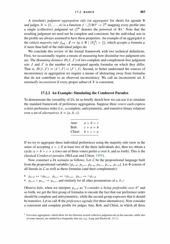
1 7 .2 basics 403
A (resolute) judgment aggregation rule (or aggregator for short) for agenda �
and judges N = {1, . . . , n} is a function f : J (�)n → 2� mapping every profile intoa single (collective) judgment set (2� denotes the powerset of �).4 Note that theresulting judgment set need not be complete and consistent, but the individual sets inthe profile are always assumed to have these properties. An example of an aggregator isthe (strict) majority rule fmaj : J �→ {ϕ ∈ � | |N J
ϕ | > n2 }, which accepts a formula ϕ
if more than half of the individual judges do.We conclude this review of the formal framework with two technical definitions.
First, we occasionally require a means of measuring how dissimilar two judgment setsare. The Hamming distance H (J, J ′) of two complete and complement-free judgmentsets J and J ′ is the number of nonnegated agenda formulas on which they differ.That is, H (J, J ′) := |J \ J ′| = |J ′ \ J |. Second, to better understand the sources ofinconsistency in aggregation we require a means of abstracting away from formulasthat do not contribute to an observed inconsistency. We call an inconsistent set X
minimally inconsistent if every proper subset of X is consistent.
17.2.2 An Example: Simulating the Condorcet Paradox
To demonstrate the versatility of JA, let us briefly sketch how we can use it to simulatethe standard framework of preference aggregation. Suppose three voters each expressa strict preference order (i.e., a complete, antisymmetric, and transitive binary relation)over a set of alternatives A = {a, b, c}:
Ann: a � b � c
Bob: c � a � b
Chloe: b � c � a
If we try to aggregate these individual preferences using the majority rule (now in thesense of accepting x � y if at least two of the three individuals do), then we obtain acycle: a � b � c � a (two out of three voters prefer a over b, and so forth). This is theclassical Condorcet paradox (McLean and Urken, 1995).
Now construct a JA scenario as follows. Let L be the propositional language builtfrom the propositional variables {pa�b, pa�c, pb�a, pb�c, pc�a, pc�b}. Let � consist ofall literals in L as well as these formulas (and their complements):
� pa�b ↔ ¬pb�a , pa�c ↔ ¬pc�a , pb�c ↔ ¬pc�b� pa�b ∧ pb�c → pa�c, and similarly for all other permutations of a, b, c
Observe how, when we interpret pa�b as “I consider a being preferable over b” andso forth, we get the first group of formulas to encode the fact that our preference ordershould be complete and antisymmetric, while the second group expresses that it shouldbe transitive. Let us call � the preference agenda (for three alternatives). Now considera consistent and complete profile for judges Ann, Bob, and Chloe, in which all three
4 Irresolute aggregators, which allow for ties between several collective judgment sets in the outcome, while alsoof some interest, are studied less frequently (but see, e.g., Lang and Slavkovik, 2013).
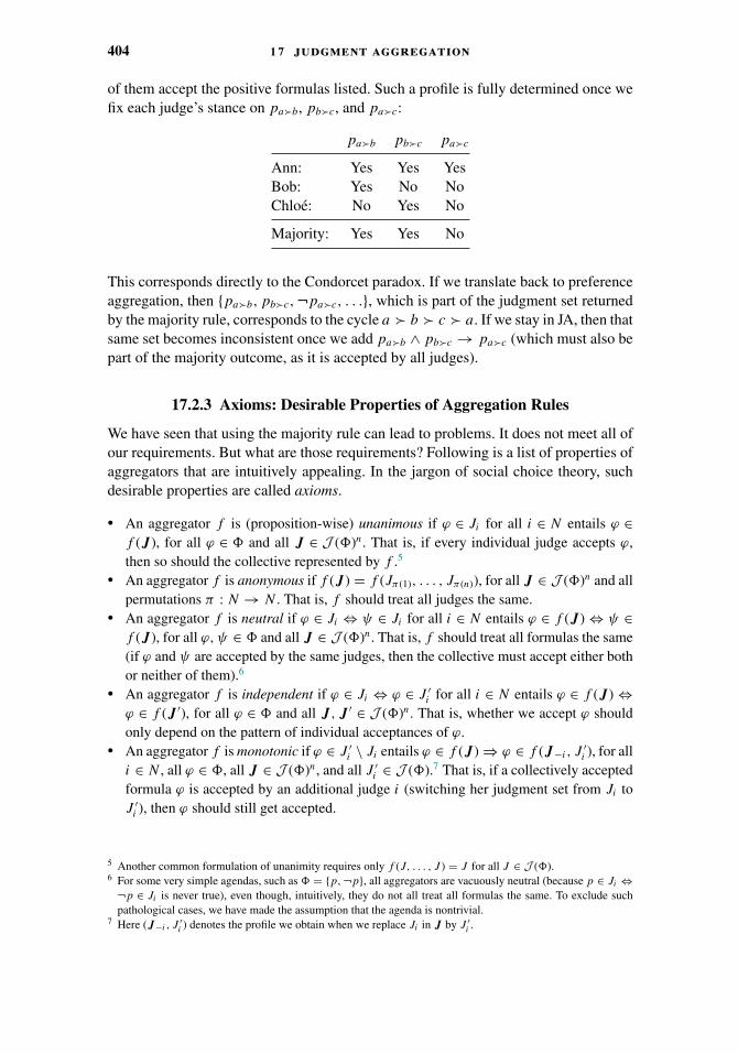
404 1 7 judgment aggregation
of them accept the positive formulas listed. Such a profile is fully determined once wefix each judge’s stance on pa�b, pb�c, and pa�c:
pa�b pb�c pa�c
Ann: Yes Yes YesBob: Yes No NoChloe: No Yes No
Majority: Yes Yes No
This corresponds directly to the Condorcet paradox. If we translate back to preferenceaggregation, then {pa�b, pb�c,¬pa�c, . . .}, which is part of the judgment set returnedby the majority rule, corresponds to the cycle a � b � c � a. If we stay in JA, then thatsame set becomes inconsistent once we add pa�b ∧ pb�c → pa�c (which must also bepart of the majority outcome, as it is accepted by all judges).
17.2.3 Axioms: Desirable Properties of Aggregation Rules
We have seen that using the majority rule can lead to problems. It does not meet all ofour requirements. But what are those requirements? Following is a list of properties ofaggregators that are intuitively appealing. In the jargon of social choice theory, suchdesirable properties are called axioms.
� An aggregator f is (proposition-wise) unanimous if ϕ ∈ Ji for all i ∈ N entails ϕ ∈f ( J), for all ϕ ∈ � and all J ∈ J (�)n. That is, if every individual judge accepts ϕ,then so should the collective represented by f .5
� An aggregator f is anonymous if f ( J) = f (Jπ(1), . . . , Jπ(n)), for all J ∈ J (�)n and allpermutations π : N → N . That is, f should treat all judges the same.
� An aggregator f is neutral if ϕ ∈ Ji ⇔ ψ ∈ Ji for all i ∈ N entails ϕ ∈ f ( J) ⇔ ψ ∈f ( J), for all ϕ,ψ ∈ � and all J ∈ J (�)n. That is, f should treat all formulas the same(if ϕ and ψ are accepted by the same judges, then the collective must accept either bothor neither of them).6
� An aggregator f is independent if ϕ ∈ Ji ⇔ ϕ ∈ J ′i for all i ∈ N entails ϕ ∈ f ( J) ⇔
ϕ ∈ f ( J ′), for all ϕ ∈ � and all J, J ′ ∈ J (�)n. That is, whether we accept ϕ shouldonly depend on the pattern of individual acceptances of ϕ.
� An aggregator f is monotonic if ϕ ∈ J ′i \ Ji entails ϕ ∈ f ( J) ⇒ ϕ ∈ f ( J−i , J
′i ), for all
i ∈ N , all ϕ ∈ �, all J ∈ J (�)n, and all J ′i ∈ J (�).7 That is, if a collectively accepted
formula ϕ is accepted by an additional judge i (switching her judgment set from Ji toJ ′
i ), then ϕ should still get accepted.
5 Another common formulation of unanimity requires only f (J, . . . , J ) = J for all J ∈ J (�).6 For some very simple agendas, such as � = {p,¬p}, all aggregators are vacuously neutral (because p ∈ Ji ⇔¬p ∈ Ji is never true), even though, intuitively, they do not all treat all formulas the same. To exclude suchpathological cases, we have made the assumption that the agenda is nontrivial.
7 Here ( J−i , J′i ) denotes the profile we obtain when we replace Ji in J by J ′
i .
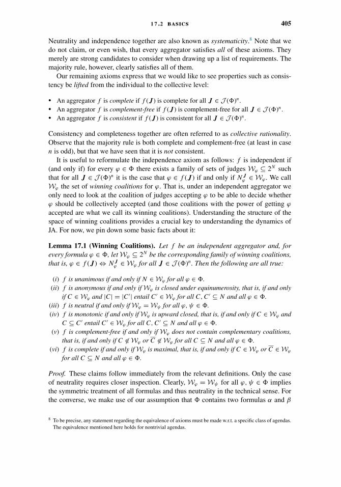
1 7 .2 basics 405
Neutrality and independence together are also known as systematicity.8 Note that wedo not claim, or even wish, that every aggregator satisfies all of these axioms. Theymerely are strong candidates to consider when drawing up a list of requirements. Themajority rule, however, clearly satisfies all of them.
Our remaining axioms express that we would like to see properties such as consis-tency be lifted from the individual to the collective level:
� An aggregator f is complete if f ( J) is complete for all J ∈ J (�)n.� An aggregator f is complement-free if f ( J) is complement-free for all J ∈ J (�)n.� An aggregator f is consistent if f ( J) is consistent for all J ∈ J (�)n.
Consistency and completeness together are often referred to as collective rationality.Observe that the majority rule is both complete and complement-free (at least in casen is odd), but that we have seen that it is not consistent.
It is useful to reformulate the independence axiom as follows: f is independent if(and only if) for every ϕ ∈ � there exists a family of sets of judges Wϕ ⊆ 2N suchthat for all J ∈ J (�)n it is the case that ϕ ∈ f ( J) if and only if N J
ϕ ∈ Wϕ . We callWϕ the set of winning coalitions for ϕ. That is, under an independent aggregator weonly need to look at the coalition of judges accepting ϕ to be able to decide whetherϕ should be collectively accepted (and those coalitions with the power of getting ϕ
accepted are what we call its winning coalitions). Understanding the structure of thespace of winning coalitions provides a crucial key to understanding the dynamics ofJA. For now, we pin down some basic facts about it:
Lemma 17.1 (Winning Coalitions). Let f be an independent aggregator and, forevery formula ϕ ∈ �, let Wϕ ⊆ 2N be the corresponding family of winning coalitions,that is, ϕ ∈ f ( J) ⇔ N J
ϕ ∈ Wϕ for all J ∈ J (�)n. Then the following are all true:
(i) f is unanimous if and only if N ∈ Wϕ for all ϕ ∈ �.(ii) f is anonymous if and only if Wϕ is closed under equinumerosity, that is, if and only
if C ∈ Wϕ and |C| = |C ′| entail C ′ ∈ Wϕ for all C,C ′ ⊆ N and all ϕ ∈ �.(iii) f is neutral if and only if Wϕ = Wψ for all ϕ,ψ ∈ �.(iv) f is monotonic if and only if Wϕ is upward closed, that is, if and only if C ∈ Wϕ and
C ⊆ C ′ entail C ′ ∈ Wϕ for all C,C ′ ⊆ N and all ϕ ∈ �.(v) f is complement-free if and only if Wϕ does not contain complementary coalitions,
that is, if and only if C �∈ Wϕ or C �∈ Wϕ for all C ⊆ N and all ϕ ∈ �.(vi) f is complete if and only if Wϕ is maximal, that is, if and only if C ∈ Wϕ or C ∈ Wϕ
for all C ⊆ N and all ϕ ∈ �.
Proof. These claims follow immediately from the relevant definitions. Only the caseof neutrality requires closer inspection. Clearly, Wϕ = Wψ for all ϕ, ψ ∈ � impliesthe symmetric treatment of all formulas and thus neutrality in the technical sense. Forthe converse, we make use of our assumption that � contains two formulas α and β
8 To be precise, any statement regarding the equivalence of axioms must be made w.r.t. a specific class of agendas.The equivalence mentioned here holds for nontrivial agendas.
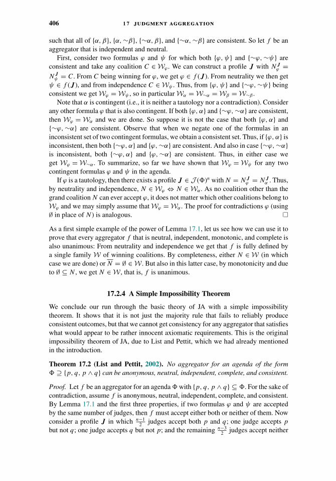
406 1 7 judgment aggregation
such that all of {α, β}, {α,∼β}, {∼α, β}, and {∼α,∼β} are consistent. So let f be anaggregator that is independent and neutral.
First, consider two formulas ϕ and ψ for which both {ϕ, ψ} and {∼ϕ,∼ψ} areconsistent and take any coalition C ∈ Wϕ . We can construct a profile J with N J
ϕ =N J
ψ = C. From C being winning for ϕ, we get ϕ ∈ f ( J). From neutrality we then getψ ∈ f ( J), and from independence C ∈ Wψ . Thus, from {ϕ, ψ} and {∼ϕ,∼ψ} beingconsistent we get Wϕ = Wψ , so in particular Wα = W∼α = Wβ = W∼β .
Note that α is contingent (i.e., it is neither a tautology nor a contradiction). Considerany other formula ϕ that is also contingent. If both {ϕ, α} and {∼ϕ,∼α} are consistent,then Wϕ = Wα and we are done. So suppose it is not the case that both {ϕ, α} and{∼ϕ,∼α} are consistent. Observe that when we negate one of the formulas in aninconsistent set of two contingent formulas, we obtain a consistent set. Thus, if {ϕ, α} isinconsistent, then both {∼ϕ, α} and {ϕ,∼α} are consistent. And also in case {∼ϕ,∼α}is inconsistent, both {∼ϕ, α} and {ϕ,∼α} are consistent. Thus, in either case weget Wϕ = W∼α . To summarize, so far we have shown that Wϕ = Wψ for any twocontingent formulas ϕ and ψ in the agenda.
If ϕ is a tautology, then there exists a profile J ∈ J (�)n with N = N Jϕ = N J
α . Thus,by neutrality and independence, N ∈ Wϕ ⇔ N ∈ Wα . As no coalition other than thegrand coalition N can ever accept ϕ, it does not matter which other coalitions belong toWϕ and we may simply assume that Wϕ = Wα . The proof for contradictions ϕ (using∅ in place of N) is analogous.
As a first simple example of the power of Lemma 17.1, let us see how we can use it toprove that every aggregator f that is neutral, independent, monotonic, and complete isalso unanimous: From neutrality and independence we get that f is fully defined bya single family W of winning coalitions. By completeness, either N ∈ W (in whichcase we are done) or N = ∅ ∈ W . But also in this latter case, by monotonicity and dueto ∅ ⊆ N , we get N ∈ W , that is, f is unanimous.
17.2.4 A Simple Impossibility Theorem
We conclude our run through the basic theory of JA with a simple impossibilitytheorem. It shows that it is not just the majority rule that fails to reliably produceconsistent outcomes, but that we cannot get consistency for any aggregator that satisfieswhat would appear to be rather innocent axiomatic requirements. This is the originalimpossibility theorem of JA, due to List and Pettit, which we had already mentionedin the introduction.
Theorem 17.2 (List and Pettit, 2002). No aggregator for an agenda of the form� ⊇ {p, q, p ∧ q} can be anonymous, neutral, independent, complete, and consistent.
Proof. Let f be an aggregator for an agenda � with {p, q, p ∧ q} ⊆ �. For the sake ofcontradiction, assume f is anonymous, neutral, independent, complete, and consistent.By Lemma 17.1 and the first three properties, if two formulas ϕ and ψ are acceptedby the same number of judges, then f must accept either both or neither of them. Nowconsider a profile J in which n−1
2 judges accept both p and q; one judge accepts p
but not q; one judge accepts q but not p; and the remaining n−32 judges accept neither
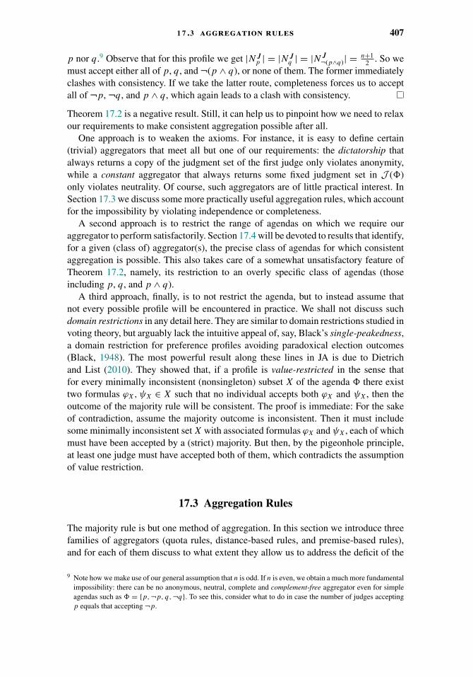
1 7 .3 aggregation rules 407
p nor q.9 Observe that for this profile we get |N Jp | = |N J
q | = |N J¬(p∧q)| = n+1
2 . So wemust accept either all of p, q, and ¬(p ∧ q), or none of them. The former immediatelyclashes with consistency. If we take the latter route, completeness forces us to acceptall of ¬p, ¬q, and p ∧ q, which again leads to a clash with consistency.
Theorem 17.2 is a negative result. Still, it can help us to pinpoint how we need to relaxour requirements to make consistent aggregation possible after all.
One approach is to weaken the axioms. For instance, it is easy to define certain(trivial) aggregators that meet all but one of our requirements: the dictatorship thatalways returns a copy of the judgment set of the first judge only violates anonymity,while a constant aggregator that always returns some fixed judgment set in J (�)only violates neutrality. Of course, such aggregators are of little practical interest. InSection 17.3 we discuss some more practically useful aggregation rules, which accountfor the impossibility by violating independence or completeness.
A second approach is to restrict the range of agendas on which we require ouraggregator to perform satisfactorily. Section 17.4 will be devoted to results that identify,for a given (class of) aggregator(s), the precise class of agendas for which consistentaggregation is possible. This also takes care of a somewhat unsatisfactory feature ofTheorem 17.2, namely, its restriction to an overly specific class of agendas (thoseincluding p, q, and p ∧ q).
A third approach, finally, is to not restrict the agenda, but to instead assume thatnot every possible profile will be encountered in practice. We shall not discuss suchdomain restrictions in any detail here. They are similar to domain restrictions studied invoting theory, but arguably lack the intuitive appeal of, say, Black’s single-peakedness,a domain restriction for preference profiles avoiding paradoxical election outcomes(Black, 1948). The most powerful result along these lines in JA is due to Dietrichand List (2010). They showed that, if a profile is value-restricted in the sense thatfor every minimally inconsistent (nonsingleton) subset X of the agenda � there existtwo formulas ϕX, ψX ∈ X such that no individual accepts both ϕX and ψX, then theoutcome of the majority rule will be consistent. The proof is immediate: For the sakeof contradiction, assume the majority outcome is inconsistent. Then it must includesome minimally inconsistent set X with associated formulas ϕX and ψX, each of whichmust have been accepted by a (strict) majority. But then, by the pigeonhole principle,at least one judge must have accepted both of them, which contradicts the assumptionof value restriction.
17.3 Aggregation Rules
The majority rule is but one method of aggregation. In this section we introduce threefamilies of aggregators (quota rules, distance-based rules, and premise-based rules),and for each of them discuss to what extent they allow us to address the deficit of the
9 Note how we make use of our general assumption that n is odd. If n is even, we obtain a much more fundamentalimpossibility: there can be no anonymous, neutral, complete and complement-free aggregator even for simpleagendas such as � = {p,¬p, q,¬q}. To see this, consider what to do in case the number of judges acceptingp equals that accepting ¬p.
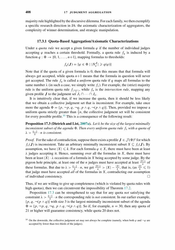
408 1 7 judgment aggregation
majority rule highlighted by the discursive dilemma. For each family, we then exemplifya specific research direction in JA: the axiomatic characterization of aggregators, thecomplexity of winner determination, and strategic manipulation.
17.3.1 Quota-Based Aggregation/Axiomatic Characterizations
Under a quota rule we accept a given formula ϕ if the number of individual judgesaccepting ϕ reaches a certain threshold. Formally, a quota rule fq is induced by afunction q : � → {0, 1, . . . , n+1}, mapping formulas to thresholds:
fq( J) = {ϕ ∈ � | |N Jϕ | � q(ϕ)}
Note that if the quota of a given formula is 0, then this means that that formula willalways get accepted, while quota n+1 means that the formula in question will neverget accepted. The rule fq is called a uniform quota rule if q maps all formulas to thesame number λ (in such a case, we simply write fλ). For example, the (strict) majorityrule is the uniform quota rule f% n+1
2 &, while fn is the intersection rule, mapping anygiven profile J to the judgment set J1 ∩ · · · ∩ Jn.
It is intuitively clear that, if we increase the quota, then it should be less likelythat we obtain a collective judgment set that is inconsistent. For example, take oncemore the agenda � = {p,¬p, q,¬q, p ∧ q,¬(p ∧ q)}. Then, provided we impose auniform quota strictly greater than 2
3n, the collective judgment set will be consistentfor every possible profile.10 This is a consequence of the following result:
Proposition 17.3 (Dietrich and List, 2007a). Let k be the size of the largest minimallyinconsistent subset of the agenda �. Then every uniform quota rule fλ with a quota ofλ > k−1
k· n is consistent.
Proof. For the sake of contradiction, suppose there exists a profile J ∈ J (�)n for whichfλ( J) is inconsistent. Take an arbitrary minimally inconsistent subset X ⊆ fλ( J). Byassumption, we have |X| � k. For each formula ϕ ∈ X, there must have been at leastλ judges accepting it. Hence, summing over all the formulas in X, there must havebeen at least |X| · λ occasions of a formula in X being accepted by some judge. By thepigeon hole principle, at least one of the n judges must have accepted at least |X|·λ
nof
these formulas. But due to λ > k−1k
· n, we get |X|·λn
> |X| − |X|k
, that is, (as |X|k
� 1)that judge must have accepted all of the formulas in X, contradicting our assumptionof individual consistency.
Thus, if we are willing to give up completeness (which is violated by quota rules withhigh quotas), then we can circumvent the impossibility of Theorem 17.2.
Proposition 17.3 can be strengthened to say that for any quota not satisfying theconstraint λ > k−1
k· n the corresponding rule is not consistent. In our earlier example,
{p, q,¬(p ∧ q)} with size 3 is the largest minimally inconsistent subset of the agenda� = {p,¬p, q,¬q, p ∧ q,¬(p ∧ q)}. So if, for example, n = 30, then any quota of21 or higher will guarantee consistency, while quota 20 does not.
10 On the downside, the collective judgment set may not always be complete (namely, when both ϕ and ∼ϕ areaccepted by fewer than two thirds of the judges).
1 7 .3 aggregation rules 409
An important question in social choice theory is whether a given set of axiomaticrequirements fully characterizes a particular aggregator (or family of aggregators). Ifthis is the case and if we have strong normative support for the axioms in question, thenthis forces us to adopt the corresponding aggregator. Let us briefly review a number ofsuch characterization results for quota rules.
Proposition 17.4 (Dietrich and List, 2007a). An aggregator is anonymous, indepen-dent, and monotonic if and only if it is a quota rule.
Proof. For the right-to-left direction, observe that every quota rule clearly has thosethree properties. For the left-to-right direction, the claim follows from Lemma 17.1: Byindependence, we can decide formula by formula. By monotonicity, the set of winningcoalitions is upward closed. By anonymity, only the size of coalitions matters. Takentogether, this means that for every formula ϕ there exists a number λϕ such that ϕ iscollectively accepted if and only if at least λϕ judges accept ϕ. In other words, λϕ isthe quota associated with ϕ, that is, q(ϕ) = λϕ .
A quota rule is neutral if and only if it is a uniform quota rule.11 Thus, as an immediateconsequence of Proposition 17.4, we obtain the following characterization:
Corollary 17.5. An aggregator is anonymous, neutral, independent, and monotonic ifand only if it is a uniform quota rule.
We now want to add completeness and complement-freeness to our requirements(but not consistency, which we already know to be impossible from Theorem 17.2).Intuitively speaking, low quotas should favor completeness (as generally more formulaswill get accepted), while high quotas should favor complement-freeness (as generallyfewer formulas will get accepted). Let λ be the uniformly imposed quota. If k individualsaccept ϕ, then n−k individuals accept ∼ϕ. Thus, to guarantee completeness, we requiremax{k, n−k} � λ for all k � n, as that way at least one of ϕ and ∼ϕ will get acceptedunder all circumstances. Similarly, to guarantee complement-freeness, we require λ >
min{k, n−k} for all k � n. The closer k is to n2 , the harder it gets to satisfy both of
these constraints. Recall that we assume n to be odd. For k = n+12 , there is only a
single value for λ that will satisfy both constraints, namely, λ = n+12 . That is, only the
majority rule satisfies all of our requirements and we obtain the following corollary toCorollary 17.5:
Corollary 17.6. An aggregator is anonymous, neutral, independent, monotonic, com-plete, and complement-free if and only if it is the (strict) majority rule.
We stress that Corollary 17.6 is true only when the number n of individual judges isodd. As pointed out in Footnote 9 already, when n is even, there exists no aggregatorthat satisfies all of these requirements. For the special case of an agenda with just asingle pair of complementary formulas, Corollary 17.6 reduces to May’s Theorem onthe characterization of the majority rule in voting theory (May, 1952).12
11 This characterization holds, provided the agenda is nontrivial. See also Footnote 6.12 May allows for ties and uses a more sophisticated monotonicity axiom, known as positive responsiveness, so
as to be able to also cover the case of an even number of individuals. Refer to Chapter 2 for full details.

410 1 7 judgment aggregation
17.3.2 Distance-based Aggregation/Winner Determination
Another approach to aggregation is to select as outcome a judgment set that, in somesense, minimizes the distance to the profile. If we measure distances between judgmentsets using the Hamming distance and if we interpret the distance from an outcome toa profile as the sum of the distances between that outcome and each of the individualjudgment sets, then we obtain the following aggregator:
fkem( J) = argminJ∈J (�)
∑i∈N
H (J, Ji).
That is, we go through all complete and consistent judgment sets J and return the onethat minimizes the sum of the Hamming distances to the individual judgment sets. Thisrule, discussed under a variety of different names in the literature, is the most widelyused distance-based aggregator in JA. If we apply it to the preference agenda (seeSection 17.2.2), then we obtain the Kemeny rule familiar from preference aggregation(Kemeny, 1959) and discussed in depth in Chapter 4 this is why we shall refer to it asthe generalized Kemeny rule. To be precise, fkem is an irresolute aggregator, as it mayreturn a set of several judgment sets (that are all equally close to the profile). To obtaina resolute rule fitting our definition of Section 17.2.1, we have to combine fkem with atie-breaking rule.
The generalized Kemeny rule is clearly consistent: only consistent judgment setsare considered as possible outcomes during the optimization process. It achieves con-sistency by sacrificing independence.
A fundamental question in computational social choice concerns the computationalcomplexity of the winner determination problem of a given method of aggregation.For a resolute aggregator f this can be cast as a decision problem by asking, fora given profile J and a given formula ϕ ∈ �, whether it is the case that ϕ ∈ f ( J).By answering this question for every formula ϕ in the agenda, we can compute theoutcome, the “winning” judgment set. Thus, the complexity of our decision problemis directly relevant to the algorithmic feasibility of the pragmatic problem of applyingrule f . For irresolute aggregators, such as the generalized Kemeny rule, an appropriateformulation of the question is whether, for a given profile J and a given set L ⊆ �,there exists a winning set J � ∈ f ( J) such that L ⊆ J �. For the generalized Kemenyrule, winner determination is highly intractable:
Theorem 17.7 (Endriss et al., 2012). The winner determination problem of the gen-eralized Kemeny rule is �P
2 -complete.
The complexity class �P2 is the class of problems that can be solved, in polynomial
time, by a (hypothetical) machine that has access to an oracle capable of decidingNP-complete problems in an instant, with the restriction that the number of queriesto the oracle must be at most logarithmic in the size of the problem. Equivalently,we may ask a polynomial number of oracle queries, provided we ask them all inparallel. That is, the generalized Kemeny rule is complete for parallel access to NP.The proof of Theorem 17.7 is beyond the scope of this chapter. It is based on a reductionfrom the Kemeny Winner problem in voting theory, for which �P
2 -completeness wasestablished by Hemaspaandra et al. (2005). For a discussion of that problem we refer
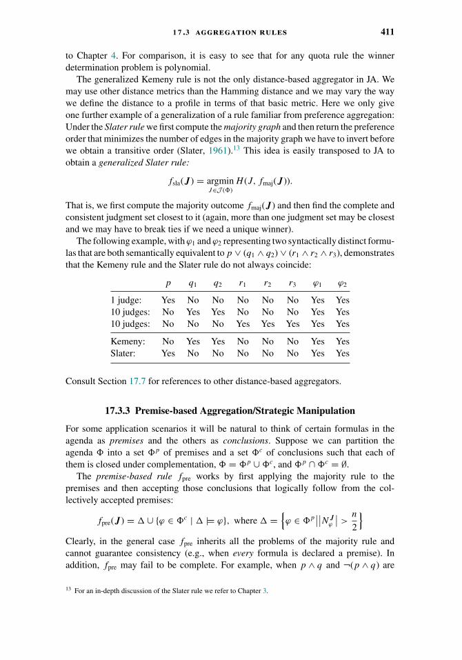
1 7 .3 aggregation rules 411
to Chapter 4. For comparison, it is easy to see that for any quota rule the winnerdetermination problem is polynomial.
The generalized Kemeny rule is not the only distance-based aggregator in JA. Wemay use other distance metrics than the Hamming distance and we may vary the waywe define the distance to a profile in terms of that basic metric. Here we only giveone further example of a generalization of a rule familiar from preference aggregation:Under the Slater rule we first compute the majority graph and then return the preferenceorder that minimizes the number of edges in the majority graph we have to invert beforewe obtain a transitive order (Slater, 1961).13 This idea is easily transposed to JA toobtain a generalized Slater rule:
fsla( J) = argminJ∈J (�)
H (J, fmaj( J)).
That is, we first compute the majority outcome fmaj( J) and then find the complete andconsistent judgment set closest to it (again, more than one judgment set may be closestand we may have to break ties if we need a unique winner).
The following example, with ϕ1 and ϕ2 representing two syntactically distinct formu-las that are both semantically equivalent to p ∨ (q1 ∧ q2) ∨ (r1 ∧ r2 ∧ r3), demonstratesthat the Kemeny rule and the Slater rule do not always coincide:
p q1 q2 r1 r2 r3 ϕ1 ϕ2
1 judge: Yes No No No No No Yes Yes10 judges: No Yes Yes No No No Yes Yes10 judges: No No No Yes Yes Yes Yes Yes
Kemeny: No Yes Yes No No No Yes YesSlater: Yes No No No No No Yes Yes
Consult Section 17.7 for references to other distance-based aggregators.
17.3.3 Premise-based Aggregation/Strategic Manipulation
For some application scenarios it will be natural to think of certain formulas in theagenda as premises and the others as conclusions. Suppose we can partition theagenda � into a set �p of premises and a set �c of conclusions such that each ofthem is closed under complementation, � = �p ∪ �c, and �p ∩ �c = ∅.
The premise-based rule fpre works by first applying the majority rule to thepremises and then accepting those conclusions that logically follow from the col-lectively accepted premises:
fpre( J) = � ∪ {ϕ ∈ �c | � |= ϕ}, where � ={ϕ ∈ �p
∣∣∣∣N Jϕ
∣∣ >n
2
}Clearly, in the general case fpre inherits all the problems of the majority rule andcannot guarantee consistency (e.g., when every formula is declared a premise). Inaddition, fpre may fail to be complete. For example, when p ∧ q and ¬(p ∧ q) are
13 For an in-depth discussion of the Slater rule we refer to Chapter 3.
412 1 7 judgment aggregation
conclusions and no premise has either p or q as a subformula, then neither p ∧ q nor¬(p ∧ q) will be logically entailed by whatever (consistent) set of premises we endup accepting. However, if we impose suitable constraints on the definition of premisesand conclusions, we can obtain a well-behaved aggregator. The most common set ofassumptions, which we shall also adopt here, is the following:
(i) The set of premises is the set of literals in the agenda.(ii) The agenda is closed under propositional variables, that is, if ϕ is a formula in the
agenda, then so is every propositional variable occurring within ϕ.
Assumption (i) guarantees consistency; a set of collectively accepted premises nowdirectly corresponds to an assignment of truth values to propositional variables.Assumption (ii) then guarantees completeness, because, for every conclusion ϕ, eitherϕ or ∼ϕ will be satisfied by that truth assignment. That is, we obtain the followingresult (given our assumption of n being odd):
Fact 17.8. For any agenda that is closed under propositional variables, the premise-based rule, with the premises being the literals, is complete and consistent.
Thus, by sacrificing both neutrality and independence, the premise-based rule allowsus to circumvent the impossibility of Theorem 17.2.
We have seen that distance-based aggregators achieve consistency at the price ofhigh computational complexity. This is not the case for fpre:
Fact 17.9. The winner determination problem of the premise-based rule, with thepremises being the literals, is polynomial.
Indeed, applying the majority rule to the premises is certainly polynomial. Decidingwhether a given conclusion should be accepted then amounts to a model checkingproblem for propositional logic, which can also be done in polynomial time.
One of the central phenomena studied in social choice theory is strategic behavior.Under what circumstances do individuals have an incentive to truthfully report theirprivate information to the aggregation mechanism? This is a very natural question inthe context of voting or resource allocation, where this private information concerns theindividuals’ preferences and where we can use these very same preferences to definewhat it means for an individual to have an incentive to perform a given action. In JA,on the other hand, individuals do not have preferences, so it is not obvious what itmay mean for an individual to have an incentive one way or the other. To be able toanalyze strategic behavior in JA, we need to endow our judges with preferences. Forthe purposes of this brief exposition, let us assume that every judge’s preferences areinduced by her true judgment set and the Hamming distance: judge i with true judgmentset Ji prefers J to J ′, denoted as J �i J ′, if and only if H (Ji, J ) < H (Ji, J
′). We saythat she has Hamming preferences.14 Now suppose three judges truthfully report theirjudgment sets:
14 Preferences induced by the Hamming distance are also discussed in Chapter 9 on voting in combinatorialdomains.
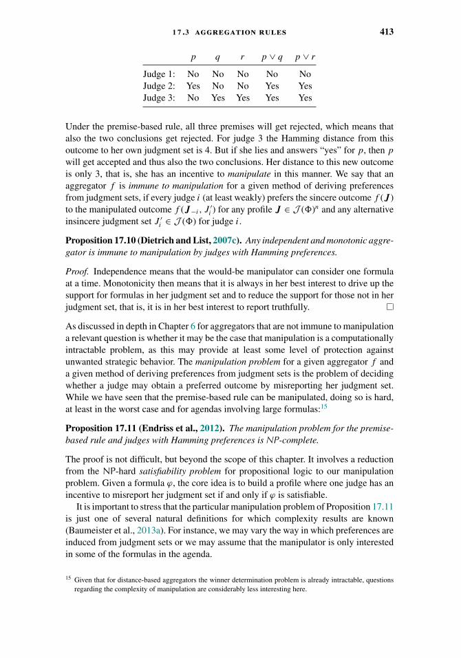
1 7 .3 aggregation rules 413
p q r p ∨ q p ∨ r
Judge 1: No No No No NoJudge 2: Yes No No Yes YesJudge 3: No Yes Yes Yes Yes
Under the premise-based rule, all three premises will get rejected, which means thatalso the two conclusions get rejected. For judge 3 the Hamming distance from thisoutcome to her own judgment set is 4. But if she lies and answers “yes” for p, then p
will get accepted and thus also the two conclusions. Her distance to this new outcomeis only 3, that is, she has an incentive to manipulate in this manner. We say that anaggregator f is immune to manipulation for a given method of deriving preferencesfrom judgment sets, if every judge i (at least weakly) prefers the sincere outcome f ( J)to the manipulated outcome f ( J−i , J
′i ) for any profile J ∈ J (�)n and any alternative
insincere judgment set J ′i ∈ J (�) for judge i.
Proposition 17.10 (Dietrich and List, 2007c). Any independent and monotonic aggre-gator is immune to manipulation by judges with Hamming preferences.
Proof. Independence means that the would-be manipulator can consider one formulaat a time. Monotonicity then means that it is always in her best interest to drive up thesupport for formulas in her judgment set and to reduce the support for those not in herjudgment set, that is, it is in her best interest to report truthfully.
As discussed in depth in Chapter 6 for aggregators that are not immune to manipulationa relevant question is whether it may be the case that manipulation is a computationallyintractable problem, as this may provide at least some level of protection againstunwanted strategic behavior. The manipulation problem for a given aggregator f anda given method of deriving preferences from judgment sets is the problem of decidingwhether a judge may obtain a preferred outcome by misreporting her judgment set.While we have seen that the premise-based rule can be manipulated, doing so is hard,at least in the worst case and for agendas involving large formulas:15
Proposition 17.11 (Endriss et al., 2012). The manipulation problem for the premise-based rule and judges with Hamming preferences is NP-complete.
The proof is not difficult, but beyond the scope of this chapter. It involves a reductionfrom the NP-hard satisfiability problem for propositional logic to our manipulationproblem. Given a formula ϕ, the core idea is to build a profile where one judge has anincentive to misreport her judgment set if and only if ϕ is satisfiable.
It is important to stress that the particular manipulation problem of Proposition 17.11is just one of several natural definitions for which complexity results are known(Baumeister et al., 2013a). For instance, we may vary the way in which preferences areinduced from judgment sets or we may assume that the manipulator is only interestedin some of the formulas in the agenda.
15 Given that for distance-based aggregators the winner determination problem is already intractable, questionsregarding the complexity of manipulation are considerably less interesting here.
414 1 7 judgment aggregation
17.4 Agenda Characterization Results
Suppose we are given an agenda � and an aggregator f . Then we may want to ask: canwe be certain that the outcome f ( J) will be consistent for every possible consistentprofile J ∈ J (�)n over this agenda?
We want to answer such questions not only for one specific agenda �, but would liketo be able to offer a full characterization of all agendas for which the answer is positive.In this section, we provide such characterizations in terms of agenda properties that tallythe structural richness of an agenda. Going beyond individual aggregators f , we alsoprove agenda characterization results for families of aggregators F , defined in terms ofthe axioms they satisfy. Such results come in two forms: existential results talk aboutconditions under which at least some aggregator in F is consistent, while universalresults establish conditions under which all aggregators in F are. For the latter, inparticular, a relevant question is how difficult it is to verify whether a given agendasatisfies certain agenda properties. Therefore, we briefly discuss the computationalcomplexity of this problem.
17.4.1 Consistent Aggregation under the Majority Rule
In the introduction we have seen that for one specific aggregator and one specificagenda, namely, the majority rule and the agenda {p,¬p, q,¬q, p ∧ q,¬(p ∧ q)},we may encounter a discursive dilemma. That is, for this agenda it is possible toconstruct a consistent profile such that the majority rule will return a judgment setthat is inconsistent. In Section 17.2.4 we have seen a generalization of this insight: theproblem persists for any aggregator belonging to an entire class of aggregators (cf.Theorem 17.2). We now want to discuss a different generalization and ask: what is theclass of agendas for which the majority rule has this deficiency?
Intuitively speaking, the discursive dilemma comes about when there is an inconsis-tent subset X ⊆ �, such that each judge accepts sufficiently few of the formulas in X
to be individually consistent, but at the same time sufficiently many to ensure that everyformula in X gathers a majority. That is, the size of inconsistent sets, or more preciselyminimally inconsistent sets, that we can build from the formulas in the agenda seemsto matter. We say that an agenda � satisfies the median property if every inconsistentsubset of � does itself have an inconsistent subset of size at most 2.16 For example, theagenda {p,¬p, q,¬q, p ∧ q,¬(p ∧ q)} does not have the median property, becauseone of its minimally inconsistent subsets, namely, {p, q,¬(p ∧ q)}, has three elements.This agenda property allows us to give a full characterization of the agendas on whichthe majority rule is consistent:
Lemma 17.12 (Nehring and Puppe, 2007). The majority rule is consistent for a givenagenda � if and only if � has the median property.
Proof. The right-to-left direction is an instance of Proposition 17.3 for k = 2, because� having the median property means that the largest minimally inconsistent subset of
16 The term median property is due to Nehring and Puppe (2007), who coined this term in the context of workon social choice theory over a class of vector spaces known as median spaces. Agendas that satisfy the medianproperty are sometimes also called simple agendas.
1 7 .4 agenda characterization results 415
� has at most size 2. For the other direction, let � be an agenda that violates the medianproperty, that is, there exists a minimally inconsistent set X = {ϕ1, . . . , ϕk} ⊆ � withk � 3. Now consider the profile J , in which judge i accepts all formulas in X exceptfor ϕ1+(i mod 3). Note that J is consistent. But the majority rule will accept all formulasin X, that is, fmaj( J) is inconsistent.
Deciding whether a given agenda has the median property is �P2 -complete (Endriss
et al., 2012). �P2 , a complexity class located at the second level of the polynomial
hierarchy, is the class of decision problems for which a certificate for a negativeanswer can be verified in polynomial time by a machine that has access to an oraclefor answering NP-complete problems in an instant. Deciding whether a quantifiedBoolean formula of the form ∀x1 · · · ∀xn∃y1 · · · ∃ymϕ is true is the canonical exampleof a problem that is complete for this class. �P
2 includes the other complexity classesfeaturing in this chapter, particularly NP and �P
2 (and this inclusion is believed, butnot known, to be proper).
Thus, we have a doubly negative result: not only do we have to restrict ourselves tohighly simplistic agendas if we want to be certain to avoid instances of the discursivedilemma (this is the import of Lemma 17.12), but on top of this determining whethera given agenda is sufficiently simplistic is very difficult.
17.4.2 Existential Agenda Characterization
Next we want to go beyond specific aggregators (such as the majority rule), and insteadprove agenda characterization results for classes of aggregators, defined in terms ofcertain axioms. For the first such result we take the axioms defining the majorityrule (cf. Corollary 17.6), except that we substantially weaken anonymity and insteadonly require that our aggregator is not a dictatorship. Formally, an aggregator f is adictatorship if there exists an individual i� ∈ N (the dictator) such that f ( J) = Ji� forevery profile J ; otherwise f is nondictatorial.17 Lemma 17.12 shows that only agendaswith the median property guarantee consistent outcomes under the majority rule. Wewill now see that, even if we allow ourselves to pick freely from the much larger classof aggregators we obtain when we replace anonymity by nondictatoriality, we cannotdo better than that.
Before we state this result formally, let us say something about the technique we aregoing to use to prove it. Recall that any independent and neutral aggregator is definedby a family W ⊆ 2N of winning coalitions (cf. Lemma 17.1). In mathematics, a set Wof subsets of a set N is called an ultrafilter if it satisfies the following three conditions(see, e.g., Davey and Priestley, 2002):18
(i) W does not include the empty set: ∅ �∈ W .(ii) W is closed under taking intersections: C ∈ W and C ′ ∈ W entail C ∩ C ′ ∈ W for
all C,C ′ ⊆ N .(iii) W is maximal: C ∈ W or C ∈ W for all C ⊆ N .
17 To appreciate that anonymity really is much stronger than nondictatoriality, observe that the former rules outall weighted majority rules, while the latter does not.
18 Sometimes being upward closed is stated as a fourth defining condition of an ultrafilter. But note that we donot need to do so, as this already follows from the other three conditions.
416 1 7 judgment aggregation
An ultrafilter is called principal if it is of the form W = {C ⊆ N | i� ∈ C} for somei� ∈ N . By a well-known fact, every ultrafilter W on a finite set N is principal (Daveyand Priestley, 2002).19 Translating back into the world of winning coalitions, thismeans that if we can show that the set W of winning coalitions corresponding to agiven (independent and neutral) aggregator f meets the three preceding conditions,then, given that the set N of judges is finite, f must be dictatorial (with the principalelement i� of the ultrafilter being the dictator).
We are now ready to prove a first important existential agenda characterizationtheorem, for a class of aggregators defined by a natural combination of axioms:
Theorem 17.13 (Nehring and Puppe, 2007). There exists a neutral, independent,monotonic, and nondictatorial aggregator that is complete and consistent for a givenagenda � if and only if � has the median property.
Proof. The right-to-left direction follows from Lemma 17.12: if � has the medianproperty, then the majority rule is consistent (and the majority rule is also neutral,independent, monotonic, nondictatorial, and complete).
The left-to-right direction in effect establishes an impossibility result. It is equivalentto the following claim: if a given neutral, independent, and monotonic aggregator f
is complete and consistent (and thus also complement-free) for a given agenda �
that violates the median property, then f must be a dictatorship. By Lemma 17.1,neutrality and independence mean that f is determined by a single family W ofwinning coalitions. Let us show that W must be an ultrafilter on N :
(i) ∅ �∈ W: If we had ∅ ∈ W , then N ∈ W by monotonicity (because ∅ ⊆ N ), which isin direct conflict with the requirement of being complement-free (as ∅ = N ).
(ii) W is closed under taking intersections: This will be the (only) part in the proofwhere we make use of the assumption that � violates the median property. Themedian property being violated means that there exists a minimally inconsistent subsetX = {ϕ1, . . . , ϕk} ⊆ � with k � 3. Take any two winning coalitions C,C ′ ∈ W . (Weneed to show that C ∩ C ′ ∈ W .) Observe that it is possible to construct a completeand consistent profile J with the following properties:� N J
ϕ1= C
� N Jϕ2
= C ′ ∪ (N \ C)� N J
ϕ3= N \ (C ∩ C ′)
� N Jϕ
= N for all with 4 � � k
That is, each judge accepts exactly k−1 of the formulas in X (which means that everyjudge is consistent). Note that N J
∼ϕ3= C ∩ C ′. Now, C being winning implies ϕ1 ∈
f ( J). By monotonicity, any superset of C ′ is winning, including C ′ ∪ (N \ C). Thelatter implies ϕ2 ∈ f ( J). Finally, from ∅ �∈ W we get N ∈ W (i.e., f is unanimous)and therefore all judges accepting all of X \ {ϕ1, ϕ2, ϕ3} entails X \ {ϕ1, ϕ2, ϕ3} ⊆
19 The proof is immediate: Let C� := ⋂C∈W C. As N is finite, we can apply (ii) inductively and obtain C� ∈ W .
By construction, C� must be the smallest element of W . If we can show that C� is a singleton, then weare done. First, by (i), C� �= ∅. Second, for the sake of contradiction, suppose |C�| � 2. Take any nonemptyproper subset C of C�. By (iii), either C ∈ W or C ∈ W . If it is the latter, then from (ii) and C� ∈ W weget C� ∩ C = C� \ C ∈ W . Hence, in either case a proper subset of C� must be an element of W . This is therequired contradiction and concludes the proof.
1 7 .4 agenda characterization results 417
f ( J). Taken together, this means X \ {ϕ3} ⊆ f ( J). Thus, to ensure consistency of theoutcome, we must have ϕ3 �∈ f ( J). But then, to ensure completeness, we are forcedto accept ∼ϕ3 ∈ f ( J). That is, we are forced to accept a formula that was acceptedby precisely the judges in the intersection C ∩ C ′. In other words, C ∩ C ′ is winning,that is, C ∩ C ′ ∈ W .
(iii) W is maximal: This follows immediately from completeness (cf. Lemma 17.1).
As N is finite, W must in fact be a principal ultrafilter. But we have already seen thatthis is equivalent to f being dictatorial, so we are done.
The ultrafilter method is very powerful. We will see one more example of its use. Ournext theorem concerns independent and unanimous aggregators. The most importantdifference is that this time we do not want to assume neutrality, that is, we cannotwork with a single family W of winning coalitions from the outset. To still makethe ultrafilter method applicable, we have to derive neutrality. As we shall see, this ispossible for agendas that are sufficiently rich. Merely violating the median property isnot sufficient: for example, if the positive formulas in the agenda are {p, q, p ∧ q, r},then the aggregator under which judge 1 dictates the outcome for {p, q, p ∧ q} and r
is decided upon by majority is nondictatorial, independent, and unanimous. That is,we require an agenda with sufficiently strong connections between its formulas to ruleout such “localized” aggregators.
Write ϕ�−→ ψ in case there exists a minimally inconsistent set X ⊆ � with ϕ,∼ψ ∈
X. This notation indicates that, in the context of the remaining formulas in X, accepting
ϕ forces us to also accept ψ . Let�=⇒ be the transitive closure of
�−→. An agenda � is
called totally blocked if ϕ�=⇒ ψ for every two formulas ϕ, ψ ∈ �.
Lemma 17.14 (Neutrality). Every unanimous and independent aggregator f that iscomplete and consistent for a totally blocked agenda � is neutral.
Proof. Let � be a totally blocked agenda and let f be a unanimous and independentaggregator that is complete and consistent for �. By independence, for each ϕ ∈ �
there exists a Wϕ ⊆ N such that ϕ ∈ f ( J) ⇔ N Jϕ ∈ Wϕ for all profiles J .
Consider two formulas ϕ, ψ ∈ � such that ϕ�−→ ψ . We show that this implies
Wϕ ⊆ Wψ : Let X be the minimally inconsistent set establishing ϕ�−→ ψ . Take any
winning coalition C ∈ Wϕ . Construct a complete and consistent profile J in which alljudges accept all of X \ {ϕ,∼ψ}, those in C also accept ϕ and ψ , and the rest alsoaccept ∼ϕ and ∼ψ . By unanimity, X \ {ϕ,∼ψ} ⊆ f ( J). Due to C ∈ Wϕ , furthermoreϕ ∈ f ( J). Hence, consistency forces ∼ψ �∈ f ( J) and thus completeness forces ψ ∈f ( J). As it was exactly the judges in C who accepted ψ , this means that C is also awinning coalition for ψ , that is, C ∈ Wψ .
Now, by induction, not only ϕ�−→ ψ implies Wϕ ⊆ Wψ , but also ϕ
�=⇒ ψ impliesWϕ ⊆ Wψ . Total blockedness means that ϕ
�=⇒ ψ for all ϕ, ψ ∈ �. Hence, Wϕ = Wψ
for all ϕ, ψ ∈ �, that is, by Lemma 17.1, f is indeed neutral.
We require one further agenda property: � is even-number-negatable if it has a mini-mally inconsistent subset X for which (X \ Y ) ∪ {∼ϕ | ϕ ∈ Y } is consistent for some
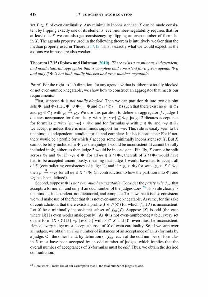
418 1 7 judgment aggregation
set Y ⊂ X of even cardinality. Any minimally inconsistent set X can be made consis-tent by flipping exactly one of its elements; even-number-negatability requires that forat least one X we can also get consistency by flipping an even number of formulasin X. The agenda property used in the following theorem is intuitively weaker than themedian property used in Theorem 17.13. This is exactly what we would expect, as theaxioms we impose are also weaker.
Theorem 17.15 (Dokow and Holzman, 2010). There exists a unanimous, independent,and nondictatorial aggregator that is complete and consistent for a given agenda � ifand only if � is not both totally blocked and even-number-negatable.
Proof. For the right-to-left direction, for any agenda � that is either not totally blockedor not even-number-negatable, we show how to construct an aggregator that meets ourrequirements.
First, suppose � is not totally blocked. Then we can partition � into two disjointsets �1 and �2 (i.e., �1 ∪ �2 = � and �1 ∩ �2 = ∅) such that there exist no ϕ1 ∈ �1
and ϕ2 ∈ �2 with ϕ1�=⇒ ϕ2. We use this partition to define an aggregator f : judge 1
dictates acceptance for formulas ϕ with {ϕ,∼ϕ} ⊆ �1; judge 2 dictates acceptancefor formulas ϕ with {ϕ,∼ϕ} ⊆ �2; and for formulas ϕ with ϕ ∈ �1 and ∼ϕ ∈ �2
we accept ϕ unless there is unanimous support for ∼ϕ. This rule is easily seen to beunanimous, independent, nondictatorial, and complete. It also is consistent: For if not,there would be a profile for which f accepts some minimally inconsistent set X. But X
cannot be fully included in �1, as then judge 1 would be inconsistent. It cannot be fullyincluded in �2 either, as then judge 2 would be inconsistent. Finally, X cannot be splitacross �1 and �2: if ∼ϕ2 ∈ �1 for all ϕ2 ∈ X ∩ �2, then all of X ∩ �2 would havehad to be accepted unanimously, meaning that judge 1 would have had to accept allof X (contradicting consistency of judge 1); and if ∼ϕ2 ∈ �2 for some ϕ2 ∈ X ∩ �2,
then ϕ1�−→ ∼ϕ2 for all ϕ1 ∈ X ∩ �1 (in contradiction to how the partition into �1 and
�2 has been defined).Second, suppose � is not even-number-negatable. Consider the parity rule fpar that
accepts a formula if and only if an odd number of the judges does.20 This rule clearly isunanimous, independent, nondictatorial, and complete. To show that it is also consistentwe will make use of the fact that � is not even-number-negatable. Assume, for the sakeof contradiction, that there exists a profile J ∈ J (�) for which fpar( J) is inconsistent.Let X be a minimally inconsistent subset of fpar( J). Suppose |X| is odd (the casewhere |X| is even works analogously). As � is not even-number-negatable, every setof the form (X \ Y ) ∪ {∼ϕ | ϕ ∈ Y } with Y ⊂ X and |Y | even must be inconsistent.Hence, every judge must accept a subset of X of even cardinality. So, if we sum overall judges, we obtain an even number of instances of an acceptance of an X-formula bya judge. On the other hand, by definition of fpar, each of the odd number of formulasin X must have been accepted by an odd number of judges, which implies that theoverall number of acceptances of X-formulas must be odd. Thus, we obtain the desiredcontradiction.
20 Here we will make use of our assumption that n, the total number of judges, is odd.
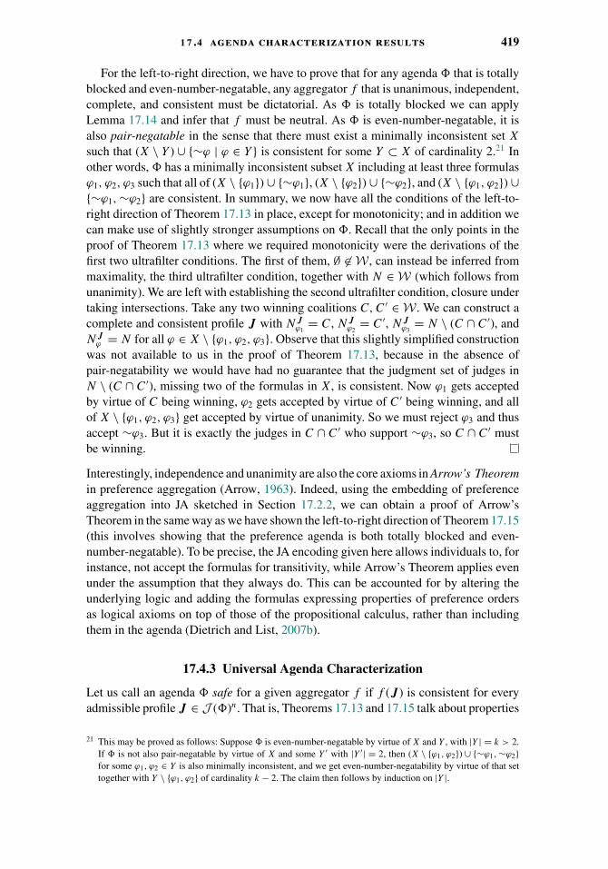
1 7 .4 agenda characterization results 419
For the left-to-right direction, we have to prove that for any agenda � that is totallyblocked and even-number-negatable, any aggregator f that is unanimous, independent,complete, and consistent must be dictatorial. As � is totally blocked we can applyLemma 17.14 and infer that f must be neutral. As � is even-number-negatable, it isalso pair-negatable in the sense that there must exist a minimally inconsistent set X
such that (X \ Y ) ∪ {∼ϕ | ϕ ∈ Y } is consistent for some Y ⊂ X of cardinality 2.21 Inother words, � has a minimally inconsistent subset X including at least three formulasϕ1, ϕ2, ϕ3 such that all of (X \ {ϕ1}) ∪ {∼ϕ1}, (X \ {ϕ2}) ∪ {∼ϕ2}, and (X \ {ϕ1, ϕ2}) ∪{∼ϕ1,∼ϕ2} are consistent. In summary, we now have all the conditions of the left-to-right direction of Theorem 17.13 in place, except for monotonicity; and in addition wecan make use of slightly stronger assumptions on �. Recall that the only points in theproof of Theorem 17.13 where we required monotonicity were the derivations of thefirst two ultrafilter conditions. The first of them, ∅ �∈ W , can instead be inferred frommaximality, the third ultrafilter condition, together with N ∈ W (which follows fromunanimity). We are left with establishing the second ultrafilter condition, closure undertaking intersections. Take any two winning coalitions C, C ′ ∈ W . We can construct acomplete and consistent profile J with N J
ϕ1= C, N J
ϕ2= C ′, N J
ϕ3= N \ (C ∩ C ′), and
N Jϕ = N for all ϕ ∈ X \ {ϕ1, ϕ2, ϕ3}. Observe that this slightly simplified construction
was not available to us in the proof of Theorem 17.13, because in the absence ofpair-negatability we would have had no guarantee that the judgment set of judges inN \ (C ∩ C ′), missing two of the formulas in X, is consistent. Now ϕ1 gets acceptedby virtue of C being winning, ϕ2 gets accepted by virtue of C ′ being winning, and allof X \ {ϕ1, ϕ2, ϕ3} get accepted by virtue of unanimity. So we must reject ϕ3 and thusaccept ∼ϕ3. But it is exactly the judges in C ∩ C ′ who support ∼ϕ3, so C ∩ C ′ mustbe winning.
Interestingly, independence and unanimity are also the core axioms in Arrow’s Theoremin preference aggregation (Arrow, 1963). Indeed, using the embedding of preferenceaggregation into JA sketched in Section 17.2.2, we can obtain a proof of Arrow’sTheorem in the same way as we have shown the left-to-right direction of Theorem 17.15(this involves showing that the preference agenda is both totally blocked and even-number-negatable). To be precise, the JA encoding given here allows individuals to, forinstance, not accept the formulas for transitivity, while Arrow’s Theorem applies evenunder the assumption that they always do. This can be accounted for by altering theunderlying logic and adding the formulas expressing properties of preference ordersas logical axioms on top of those of the propositional calculus, rather than includingthem in the agenda (Dietrich and List, 2007b).
17.4.3 Universal Agenda Characterization
Let us call an agenda � safe for a given aggregator f if f ( J) is consistent for everyadmissible profile J ∈ J (�)n. That is, Theorems 17.13 and 17.15 talk about properties
21 This may be proved as follows: Suppose � is even-number-negatable by virtue of X and Y , with |Y | = k > 2.If � is not also pair-negatable by virtue of X and some Y ′ with |Y ′| = 2, then (X \ {ϕ1, ϕ2}) ∪ {∼ϕ1,∼ϕ2}for some ϕ1, ϕ2 ∈ Y is also minimally inconsistent, and we get even-number-negatability by virtue of that settogether with Y \ {ϕ1, ϕ2} of cardinality k − 2. The claim then follows by induction on |Y |.
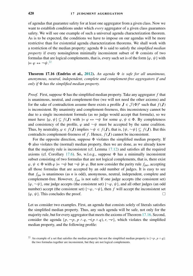
420 1 7 judgment aggregation
of agendas that guarantee safety for at least one aggregator from a given class. Now wewant to establish conditions under which every aggregator of a given class guaranteessafety. We will see one example of such a universal agenda characterization theorem.As is to be expected, the conditions we have to impose on our agendas will be morerestrictive than for existential agenda characterization theorems. We shall work witha restriction of the median property: agenda � is said to satisfy the simplified medianproperty if every nonsingleton minimally inconsistent subset of � consists of twoformulas that are logical complements, that is, every such set is of the form {ϕ, ψ} with|= ϕ ↔ ¬ψ .22
Theorem 17.16 (Endriss et al., 2012). An agenda � is safe for all unanimous,anonymous, neutral, independent, complete and complement-free aggregators if andonly if � has the simplified median property.
Proof. First, suppose � has the simplified median property. Take any aggregator f thatis unanimous, neutral, and complement-free (we will not need the other axioms) andfor the sake of contradiction assume there exists a profile J ∈ J (�)n such that f ( J)is inconsistent. By unanimity and complement-freeness, this inconsistency cannot bedue to a single inconsistent formula (as no judge would accept that formula), so wemust have {ϕ, ψ} ⊆ f ( J) with |= ϕ ↔ ¬ψ for some ϕ, ψ ∈ �. By completenessand consistency of the profile, ϕ and ∼ψ must be accepted by the same coalition.Thus, by neutrality, ϕ ∈ f ( J) implies ∼ψ ∈ f ( J), that is, {ψ,∼ψ} ⊆ f ( J). But thiscontradicts complement-freeness of f . Hence, f ( J) cannot be inconsistent.
For the opposite direction, suppose � violates the simplified median property. If� also violates the (normal) median property, then we are done, as we already knowthat the majority rule is inconsistent (cf. Lemma 17.12) and satisfies all the requiredaxioms (cf. Corollary 17.6). So, w.l.o.g., suppose � has a minimally inconsistentsubset consisting of two formulas that are not logical complements, that is, there existϕ, ψ ∈ � with ϕ |= ¬ψ but ¬ψ �|= ϕ. But now consider the parity rule fpar, acceptingall those formulas that are accepted by an odd number of judges. It is easy to seethat fpar is unanimous (as n is odd), anonymous, neutral, independent, complete andcomplement-free. However, fpar is not safe: If one judge accepts (the consistent set){ϕ,∼ψ}, one judge accepts (the consistent set) {∼ϕ, ψ}, and all other judges (an oddnumber) accept (the consistent set) {∼ϕ,∼ψ}, then f will accept the inconsistent set{ϕ, ψ}. This concludes the proof.
Let us consider two examples. First, an agenda that consists solely of literals satisfiesthe simplified median property. Thus, any such agenda will be safe, not only for themajority rule, but for every aggregator that meets the axioms of Theorem 17.16. Second,consider the agenda {p,¬p, p ∧ q,¬(p ∧ q), r,¬r}, which violates the simplifiedmedian property, and the following profile:
22 An example of a set that satisfies the median property but not the simplified median property is {¬p, p ∧ q}:the two formulas together are inconsistent, but they are not logical complements.
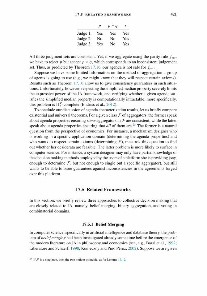
1 7 .5 related frameworks 421
p p ∧ q r
Judge 1: Yes Yes YesJudge 2: No No YesJudge 3: Yes No Yes
All three judgment sets are consistent. Yet, if we aggregate using the parity rule fpar,we have to reject p but accept p ∧ q, which corresponds to an inconsistent judgementset. Thus, as predicted by Theorem 17.16, our agenda is not safe for fpar.
Suppose we have some limited information on the method of aggregation a groupof agents is going to use (e.g., we might know that they will respect certain axioms).Results such as Theorem 17.16 allow us to give consistency guarantees in such situa-tions. Unfortunately, however, respecting the simplified median property severely limitsthe expressive power of the JA framework, and verifying whether a given agenda sat-isfies the simplified median property is computationally intractable; more specifically,this problem is �P
2 -complete (Endriss et al., 2012).To conclude our discussion of agenda characterization results, let us briefly compare
existential and universal theorems. For a given class F of aggregators, the former speakabout agenda properties ensuring some aggregators in F are consistent, while the latterspeak about agenda properties ensuring that all of them are.23 The former is a naturalquestion from the perspective of economics. For instance, a mechanism designer whois working in a specific application domain (determining the agenda properties) andwho wants to respect certain axioms (determining F), must ask this question to findout whether her desiderata are feasible. The latter problem is more likely to surface incomputer science. For instance, a system designer may only have partial knowledge ofthe decision making methods employed by the users of a platform she is providing (say,enough to determine F , but not enough to single out a specific aggregator), but stillwants to be able to issue guarantees against inconsistencies in the agreements forgedover this platform.
17.5 Related Frameworks
In this section, we briefly review three approaches to collective decision making thatare closely related to JA, namely, belief merging, binary aggregation, and voting incombinatorial domains.
17.5.1 Belief Merging
In computer science, specifically in artificial intelligence and database theory, the prob-lem of belief merging had been investigated already some time before the emergence ofthe modern literature on JA in philosophy and economics (see, e.g., Baral et al., 1992;Liberatore and Schaerf, 1998; Konieczny and Pino Perez, 2002). Suppose we are given
23 If F is a singleton, then the two notions coincide, as for Lemma 17.12.

422 1 7 judgment aggregation
several knowledge bases encoding knowledge provided by experts in a logical languageand we want to integrate these individual bases to obtain a large overall knowledgebase. The naıve approach of simply taking the union of all individual bases will, in mostcases, lead to an inconsistent knowledge base. One possible refinement is to choosea maximally consistent subset of the union (Baral et al., 1992), but this and similarapproaches do not track which individual provided which formulas in the knowledgebase, that is, it is not possible to give equal weight to different individuals. The latteris possible using distance-based procedures (Konieczny and Pino Perez, 2002), whichare also briefly discussed in Chapter 9.
There are important differences between JA and typical work in belief merging. In JAwe have an agenda and we usually assume that every individual expresses a judgmentregarding every formula in the agenda, while in belief merging the knowledge/beliefbases coming from distinct individuals need not concern the same set of formulas.Furthermore, in JA we (implicitly) impose the same constraints on different individualsand the collective, while in belief merging we typically impose an integrity constraintto be satisfied by the merged base that need not be satisfied by every individual base.Like in JA, work in belief merging often evokes the notion of “axiom” to define whatmakes a good procedure for merging, but most of the axioms used in the literature areinspired by work in belief revision (and typically are “outcome-oriented,” talking aboutconsistency requirements) rather than social choice theory (where axioms tend to havemore of an “agent-oriented” flavor).
17.5.2 Binary Aggregation
Binary aggregation (see, e.g., Dokow and Holzman, 2010; Grandi and Endriss, 2013)has its origins in the work of Wilson (1975) and Rubinstein and Fishburn (1986) onabstract (algebraic) aggregation. In binary aggregation, each individual is asked tosupply a vector of 0’s and 1’s of some fixed length, and we then have to aggregatethis information into a single such vector. The application domain under considerationdetermines which vectors are feasible. This is very closely related to the formula-basedframework of JA we have discussed in this chapter. For example, if the set of feasiblevectors is {000, 010, 100, 111}, then this induces the same domain of aggregation asthe agenda formulas p, q, and p ∧ q. In fact, in the literature the term “judgmentaggregation” is sometimes taken to encompass both JA in the narrow sense (i.e.,formula-based JA) and binary aggregation.
In the economics literature the set of feasible vectors is usually assumed to bespecified explicitly (Dokow and Holzman, 2010), while in the computer science liter-ature the set of feasible vectors is usually defined implicitly by means of an integrityconstraint expressed in the language of propositional logic (Grandi and Endriss,2013). For example, the integrity constraint x1 ∧ x2 ∧ x3 ↔ x4 defines the domain{0000, 0010, 0100, 0110, 1000, 1010, 1100, 1111}. The advantage of using integrityconstraints is that they provide a compact representation of the domain of aggrega-tion, which is important when we are interested in algorithmic aspects of aggregation.Integrity constraints also allow for alternative characterizations of aggregators. Forinstance, an aggregator is unanimous if and only if it maps feasible profiles to feasibleoutcomes for every integrity constraint expressible as a conjunction of literals; and

1 7 .6 applications in computer science 423
the only aggregators that “lifts” all possible integrity constraints in this sense are thegeneralized dictatorships, that is, those aggregators that amount to first selecting oneof the individuals and then copying that individual’s input vector to produce the output(Grandi and Endriss, 2013).
17.5.3 Voting in Combinatorial Domains
When voting on complex matters, such as the composition of a committee or theoutcome of a referendum involving a set of proposals, each of which has to be eitheraccepted or rejected, we face problems not dissimilar to those faced in JA. In sucha multiattribute election we have a number of variables, each ranging over a finitedomain, and we ask each voter for her preferences regarding the assignment of valuesto these variables. For instance, in the committee example the variables are the seatson the committee and the values are the candidates. When each variable is binary (as isthe case for referenda), we obtain a similar problem as in binary aggregation. However,a crucial difference is that in binary aggregation we assume that each individual canonly communicate one vector (i.e., one set of variable assignments), while in generalwe may ask each individual to report a complex preference structure over the set of allpossible outcomes. This raises interesting questions, not only regarding the aggregationof such information, but also regarding the compact representation of the preferencesthemselves.
Such questions are studied in the field of voting in combinatorial domains. Chapter 9is devoted to this important topic.
17.6 Applications in Computer Science
In the introduction we have already alluded to the fact that JA has important applica-tions in analytical jurisprudence and political philosophy. We want to conclude thischapter with a few words about possible applications in computer science. Maybe themost important of these, and certainly the one most often quoted as an example, iscollective decision making in systems of autonomous software agents. In such a multi-agent system we have several agents, which may have been designed and programmedby different developers and which may act on behalf of different users, and theseagents need to interact, both cooperating and competing with each other. Social choicetheory is part of the basic repertoire available for modeling the fundamental features ofmultiagent systems (Wooldridge, 2009; Shoham and Leyton-Brown, 2009). Given thatimportant aspects of the agents themselves, such as their beliefs or goals, are often rep-resented using logic, JA is a useful formalism for modeling agreements made by thoseagents.
Another important formal tool for modeling the dynamics of multiagent systems isthe theory of abstract argumentation, widely studied in artificial intelligence, whichis concerned with high-level representations of the relationships that hold betweenarguments for and against a given position. Given a network of arguments together withinformation on which argument attacks which other argument, different agents mayhold competing views on which arguments to accept. JA then is a useful framework for

424 1 7 judgment aggregation
modeling the process of finding a common view in such situations (see, e.g., Caminadaand Pigozzi, 2011).
Besides multiagent systems, another potential application for JA is informa-tion merging, for example, the merging of knowledge bases provided by dif-ferent experts briefly discussed in Section 17.5.1. This includes the merging ofontologies, which play a central role in the development of the Semantic Web(Porello and Endriss, 2011).
JA and particularly the closely related binary aggregation are also relevant to crowd-sourcing. Several areas in or related to computer science, such as, computer vision orcomputational linguistics, rely on the availability of annotated data, such as imageslabeled with object names or text corpora annotated with semantic information. Crowd-sourcing platforms provide fast and cheap means for labeling large amounts of datausing nonexpert annotators. The annotations provided by different workers then needto be aggregated to obtain a collective annotation, a task that shares many similaritieswith JA (Endriss and Fernandez, 2013).
It is important to stress that, at the time of writing, none of the applications of JAsketched here has been developed in depth. Still, JA certainly holds great potential forthese, as well as other, areas of computer science.
17.7 Bibliographic Notes and Further Reading
In this section we supply additional bibliographic references and explanations regardingsome of the material covered in this chapter. We also provide pointers to further readingon specific topics. Let us begin by pointing out that, while research on JA proper startedwith the work of List and Pettit (2002), the work of Guilbaud (1952) on what he called“the logical problem of aggregation” may be considered an early precursor of JA(Eckert and Monjardet, 2010).
Following the publication of the original impossibility theorem of List and Pettit(our Theorem 17.2), several other authors derived technically stronger results of asimilar nature, replacing in particular anonymity by absence of dictatorships (see, e.g.,Pauly and van Hees, 2006; Dietrich, 2007). Gardenfors (2006) showed that giving upthe requirement of completeness amounts to moving from dictatorships to oligarchicaggregators, that is, aggregators where the outcome is the set of those propositions afixed set of individuals completely agrees on (dictatorships and the intersection ruleare extreme cases of such oligarchic rules). We refer to List (2012) for a systematicdiscussion on how to cope with impossibility results by relaxing certain desiderata,and to Grossi and Pigozzi (2014) for an in-depth discussion of proofs of impossibilityresults using the ultrafilter method.
In work integrating the classical axiomatic method with ideas from computer sci-ence, Nehama (2013) showed that relaxing the cornerstones of most impossibilitytheorems, consistency and independence, to approximate variants of these desideratadoes not allow us to significantly improve on known negative results.
The simulation of preference aggregation in JA sketched in Section 17.2.2 followsDietrich and List (2007b), who for notational convenience use predicate rather than
1 7 .7 bibliographic notes and further reading 425
just propositional logic (which, as we have seen, is not technically required). Also theidea of deriving Arrow’s Theorem from results in JA, as briefly mentioned at the endof the Section 17.4.2, is due to Dietrich and List (2007b).
While initial work in JA had focused on impossibility results and the axiomaticmethod, work on the design of concrete practically useful methods of aggregation onlystarted several years later. Distance-based methods originally entered JA via the fieldof belief merging (Revesz, 1997; Konieczny and Pino Perez, 2002; Pigozzi, 2006). Wehave only discussed two such methods here; several others are analyzed in the workof Miller and Osherson (2009), Lang et al. (2011), and Lang and Slavkovik (2013).The premise-based rule has been part of the JA literature from the very beginning,due to its importance in the context of legal decision making in practice (Kornhauserand Sager, 1993). Other approaches for designed JA rules not discussed here includesupport-based methods (Lang et al., 2011; Porello and Endriss, 2011; Everaere et al.,2014), where aggregation is guided by the numbers of judges accepting a given formula,methods inspired by scoring rules in voting theory (Dietrich, 2014), and methods thatcopy the choice of the judge that, in some sense, is the “most representative” in thegroup (Endriss and Grandi, 2014).
The analysis of strategic behavior is a major topic in social choice theory. As we havediscussed in Section 17.3.3, how to best model an individual’s preferences, and thusher incentives, is debatable in JA. Our definition of strategic manipulation in terms ofpreferences induced by the Hamming distance is but one possibility (Dietrich and List,2007c; Baumeister et al., 2013b). Manipulation is not the only type of strategic behaviorof interest in JA. Baumeister et al. (2011) have initiated a study of the computationalcomplexity of related problems in JA, namely, bribery and control problem. For theformer, we ask whether a given budget suffices to bribe sufficiently many judges toobtain a particular outcome. An example for a control problem is the question ofwhether we can obtain a given outcome by removing at most k judges. Alon et al.(2013) have focussed on a specific control problem, where we ask whether a desiredoutcome can be enforced by conducting separate elections for certain subsets of theagenda.
In Section 17.4, we have seen that the normal and the simplified median propertyare both �P
2 -complete (Endriss et al., 2012). For most other commonly used agendaproperties, at the time of writing, no complexity results are known.
The agenda characterization results in Section 17.4.2 have been adapted to ourframework of formula-based JA from original results in binary aggregation (Dokow andHolzman, 2010) and the “property space” formulation of abstract aggregation (Nehringand Puppe, 2007). For a comprehensive review of existential agenda characterizationresults we refer to List and Puppe (2009). The ultrafilter method we employed inSection 17.4.2 is useful also in other areas of social choice theory, where it waspioneered by Kirman and Sondermann (1972).
Finally, JA uses logic to define the structure of the domain of aggregation. Abroader review of uses of logic in computational social choice, for example, to describeproperties of aggregators in a logical language or to use techniques from automatedreasoning to support the verification or discovery of results in social choice theory, isavailable elsewhere (Endriss, 2011).

426 1 7 judgment aggregation
Acknowledgments
I would like to thank Dorothea Baumeister, Franz Dietrich, Roosmarijn Goldbach,Umberto Grandi, Davide Grossi, Jerome Lang, and Daniele Porello for their helpfulfeedback on earlier versions of this chapter.
CHAPTER 18
The Axiomatic Approach andthe Internet
Moshe Tennenholtz and Aviv Zohar
18.1 Introduction
The Internet reinforces types of multiagent systems which can effectively utilize thisnew media. Reputation systems, ranking systems, trust systems, recommendation sys-tems, affiliate marketing in social networks, and more, are flowering in its midst. Thisrecent wave of online social systems is typically associated with a large amount of datathat is collected online, which leads to the “big data” approach to the utilization ofsuch information. Quite surprisingly, however, the abundance of available data does nothelp system designers to come up with the right design for online systems in the firstplace. Indeed, available data is typically generated by the use of a particular system,and mining the data generated by users while interacting with one system does notprovide a tool for exploring the overwhelmingly large design space. Interestingly, themain practical approach to software and hardware design, the formal specification ofclear system requirements and the implementation of a system satisfying these exactrequirements, has not been used often. This classical approach, when adapted to thecontext of multiagent systems, coincides with extensions of a standard tool of socialchoice theory and cooperative game theory, namely, the axiomatic approach.
The use of axioms can be either in a descriptive or in a normative context. In bothcases basic properties of a system are phrased as axioms. In the descriptive approacha basic set of properties of a known system is sought out, with the aim of finding onethat characterizes the system uniquely, hence teaching us much about its essence. Thenormative approach, on the other hand, starts from a specification of a basic set ofrequirements which is followed by an attempt to construct a system that satisfies them.Our goal in this chapter is to demonstrate both approaches in the context of the Internet.
Perhaps the best known axiomatic theory in the social sciences is the theory ofsocial choice. In the classical social choice setting we have a set of voters and a setof alternatives, where each voter has a ranking over the set of alternatives, and ouraim is to find a good aggregation of the individual rankings into a global (or social)ranking. Various properties of such aggregation functions have been considered andhave led to different characterizations of particular systems as well as impossibility
427
428 1 8 the axiomatic approach and the internet
results showing no system can satisfy certain sets of properties all at once. In theInternet setting, the study of ranking and reputation systems, such as page-rankingsystems, defines a natural extension of classical social choice to the case where the setof voters and the set of alternatives coincide. For example, in graph ranking systems,one wishes to obtain a ranking of the nodes based on the structure of the graph. Inthis case, the nodes in the graph serve the dual role of both the voters and of theobjects being ranked, with their outgoing edges determining their votes. In a particularapplication, the nodes can represent Internet pages and the search for an aggregatedordering of the pages is in fact the page ranking problem. The edges which are formedfrom the links between the pages represent votes in support of the page being linkedto. In such a setting the classical axioms of social choice become less relevant, and arereplaced with new axioms which lead to a completely new theory. Indeed, we willuse the axiomatic approach in the context of graph ranking systems, applicable topage ranking algorithms, as our first illustrative study. In particular, we will present anaxiomatic treatment of the classical PageRank algorithm.
Further removed from direct extensions of social choice, one can find systemsoriginating from personalized versions of ranking and reputation systems. Here weno longer consider the aggregation of preferences into a global or social ranking,but instead seek to provide personalized rankings or recommendations to each agent.Such recommendations are still aggregate measures, based on trust between agentsand their own local rankings. Examples of these extensions include trust systems inwhich we aim to derive an agent’s trust toward other agents he does not directlyknow based on the aggregate of localized trust-relationships between agents in thesystem. The designer is then faced with questions like the following that define theway trust should be used in the system: Who should an agent trust more, a participantwhich is unknown to others and whom the agent alone trusts directly, or an agentwho is trusted only indirectly but by many trustworthy sources? Perhaps even moreinterestingly, what is the best way to aggregate both measures of trust and of preference?Based on trust-relationships among the agents, and their expressed opinions about aservice or a product, we may be interested in trust-based recommendation systems,in which a recommendation about a service or a product is provided to agents whodid not evaluate it personally. The puzzling challenge of generating useful trust-basedrecommendation systems is amenable to an axiomatic treatment, beginning with anattempt to characterize the systems satisfying different sets of desired properties. Wewill use trust-based recommendation systems as our second illustrative study as theyshow how the spirit of axiomatic social choice can be brought into personalized systemsand not only to global preference aggregation.
In addition to the two application areas mentioned earlier, other domains for whichaxiomatic approaches have been suggested can be viewed as extensions of topics typ-ically covered in cooperative game theory. Cooperative game theory typically dealswith issues such as the distribution of monetary gains or the attribution of credit toparticipating agents. Traditional solution concepts used in cooperative games such asthe Shapley value, which originate from a purely axiomatic treatment, aim to tacklesuch issues. These, however, do not immediately extend to the design of practicalincentive and credit distribution systems that are found in some of the emerging set-tings on the Internet. An illuminating study in this context is the axiomatic approach
1 8 .2 an axiomatic characterization of pagerank 429
to multilevel marketing (also known as affiliate marketing). In this form of marketing,which is facilitated by social networks, products may be sold through referrals gener-ated by previous customers. Affiliate marketing systems offer credit in exchange forsuch referrals (especially for successful ones). We will use the axiomatic approach tomultilevel marketing as our third illustrative study.
In this chapter we have selected to focus on the preceding illustrative studies,showing technical details of the related axiomatic approaches, but omitting most ofthe proofs. We add some informal discussion of complementary treatments such as thenormative approach to ranking systems and axiomatic treatments of personalized trustsystems at the end of the chapter.
We believe the axiomatic approach is one of the fundamental messages theory bringsto the flowering industry designing Internet mechanisms in the multiagent context.While the recent trend in the research and design of social systems is to employ datamining heavily because “data is everywhere,” this approach alone is not informativeenough to design new systems from scratch, but rather leads to ad-hoc design that isonly incrementally improved by mining data and revising the system. The axiomaticapproach is a solid complementary alternative, and the illustration of its power in thepreceding settings, augmented with its conceptual depth, provides clear evidence forthat.
18.2 An Axiomatic Characterization of PageRank
The ranking of agents based on other agents’ input is fundamental to Internet-basedsystems (see, e.g., Resnick et al., 2000), and has become a central ingredient of avariety of sites, where perhaps the most famous examples are Google’s PageRankalgorithm (Page et al., 1998) which ranks web pages, and eBay’s reputation sys-tem (Resnick and Zeckhauser, 2001) in which both buyers and sellers are ranked basedon trustworthiness.
In the classical theory of social choice, as manifested by Arrow (1950), a set ofvoters is called upon to rank a set of alternatives. Given the agents’ input, that is, theagents’ individual rankings, a social ranking of the alternatives is generated. The theorystudies desired properties of the aggregation of agents’ rankings into a social ranking.
The setting of ranking systems introduces a new social choice model. The novelfeature of this setting is that the set of agents and the set of alternatives coincide.Therefore, in such a setting one may need to consider the transitive effects of voting.For example, if agent a reports on the importance of (i.e., votes for) agent b then thismay influence the credibility of a report by b on the importance of agent c; these indirecteffects should be considered when we wish to aggregate the information provided bythe agents into a social ranking.
A natural interpretation of this setting is the ranking of Internet pages. In this case,the set of agents represents the set of Internet pages, and the links from a page p
to a set of pages Q can be viewed as a two-level ranking where agents in Q arepreferred by p over pages which are not in Q. The problem of finding an appropriatesocial ranking in this case is in fact the problem of (global) page ranking. Particularapproaches for obtaining a useful page ranking and to quantify the so called importance
430 1 8 the axiomatic approach and the internet
of web pages using the link structure have been implemented by search engines (Pageet al., 1998).
Due to Arrow-like impossibility results and inspiration from the page ranking set-ting, we limit the discussion to ranking systems in which agents have dichotomouspreferences (see Bogomolnaia et al., 2005, for a discussion in the social choice set-ting). In these settings agents have only two levels of preferences: either they vote forsome agent, or they do not.
18.2.1 Ranking Systems
We begin by formally defining the term “ranking system” in the context of graphs andlinear orderings:
Definition 18.1. Let A be some set. A relation R ⊆ A × A is called a linear orderingon A if it is reflexive, transitive, antisymmetric, and complete. Let L(A) denote the setof all linear orderings on A.
Notation 18.1. Let / be a linear ordering, then ∼ is the equality predicate of /, and≺ is the strict order induced by /. Formally, a ∼ b if and only if a / b and b / a; anda ≺ b if and only if a / b but not b / a.
Given the preceding, we can define a ranking system f , which for each graph G
generates a ranking of its vertices.
Definition 18.2. Let GV be the set of all directed graphs G = (V, E) with no paralleledges, but possibly with self-loops. A ranking system f is a functional that for everyfinite vertex set V maps graphs G ∈ GV to corresponding orderings /f
G∈ L(V ).
18.2.2 PageRank
In this section we present the PageRank algorithm, which among its many other usesforms the basis for Google’s search technology1 (Brin and Page, 1998).
The current practice of the ranking of Internet pages is based on the idea of computingthe limit stationary probability distribution of a random walk on the Internet graph,where the nodes are pages, and the edges are links among the pages. Roughly speaking,page p1 will be ranked higher than page p2 if the probability of reaching p1 is greaterthan the probability of reaching p2.
The version of PageRank we present is slightly idealized form of the originalalgorithm. In its original form, small adaptations were included to deal with verticeswithout outgoing edges (sinks, and dangling vertices as they were called). In particular,in order for the result of that process to be well defined, we restrict our attention tostrongly connected aperiodic graphs in which such corrections are not necessary.2
1 Its use can indeed be found in other contexts. See Pinski and Narin (1976) for the use of PageRank-like procedurein the comparison of journals’ impact, or Newman (2008) for its use as a measure of centrality in social networkanalysis studies.
2 A graph is aperiodic if the greatest common divisor of its circles’ lengths is 1. This is a common restrictionwhich guarantees, along with strong connectivity, a unique limiting distribution for the Markov chain definedby the random walk process on a finite graph.
1 8 .2 an axiomatic characterization of pagerank 431
Definition 18.3. A directed graph G = (V, E) is called strongly connected if for allvertices v1,v2 ∈ V there exists a path from v1 to v2 in E.
In order to define the PageRank ranking system, we first recall the following standarddefinitions:
Definition 18.4. Let G = (V, E) be a directed graph, and let v ∈ V be a vertex in G.Then: The successor set of v is SG(v) = {u|(v, u) ∈ E}, and the predecessor set of v
is PG(v) = {u|(u, v) ∈ E}.We now define the PageRank matrix which is the matrix which captures the random
walk created by the PageRank procedure. Namely, in this process we start in a randompage, and iteratively move to one of the pages that are linked to by the current page,assigning equal probabilities to each such page.
Definition 18.5. Let G = (V, E) be a directed graph, and assume V = {v1, v2, . . . , vn}.the PageRank Matrix AG (of dimension n × n) is defined as:
[AG]i,j ={
1/|SG(vj )| (vj , vi) ∈ E
0 Otherwise.
The PageRank procedure will rank pages according to the stationary probabilitydistribution obtained in the limit of the preceding random walk; this is formally definedas follows:
Definition 18.6. Let G = (V, E) be some strongly connected graph, and assume V ={v1, v2, . . . , vn}. Let r be the unique solution of the system AG · r = r where r1 = 1.3
The PageRank PRG(vi) of a vertex vi ∈ V is defined as PRG(vi) = ri . The PageRankranking system is a ranking system that for the vertex set V maps G to /PR
G , where/PR
G is defined as: for all vi, vj ∈ V : vi /PRG vj if and only if PRG(vi) � PRG(vj ).
The preceding defines a powerful heuristic for the ranking of Internet pages, asadopted by search engines (Page et al., 1998). This is, however, a particular numericprocedure, and another may have been chosen in its stead. We therefore treat the generalquestion from an axiomatic social choice perspective, providing a graph-theoretic,ordinal representation theorem for PageRank.
18.2.3 The PageRank Axioms
From the perspective of the theory of social choice, each page in the Internet graphis viewed as an agent, where this agent prefers the pages (i.e., agents) it links to overpages it does not link to. The problem of finding a social aggregation rule will thereforebecome the problem of page ranking. The idea is to search for simple axioms, that is,requirements we wish the page ranking system to satisfy. Most of these requirementswill have the following structure: page a is preferable to page b when the graph is G
if and only if a is preferable to b when the graph is G′. Our aim is to exhibit a small
3 The solution is unique up to a scaling factor that can be applied to both sides of the equation. This is guaranteedfor finite, strongly connected aperiodic graphs.
432 1 8 the axiomatic approach and the internet
a
b
c
a
b
c
(a) Vote by Committee
a
b
a
(b) Collapsing
=
=x
(c) Proxy
Figure 18.1. Sketch of several axioms.
set of axioms that can be shown to be satisfied by PageRank. The axioms will thus besimple graph-theoretic, ordinal properties.
In explaining some of the axioms we will refer to Figure 18.1. For simplicity, whilethe axioms are stated as “if and only if” statements, we will sometimes emphasize inthe intuitive explanation of an axiom only one of the directions (in all cases similarintuitions hold for the other direction).
The first axiom is straightforward:
Axiom 18.2 (Isomorphism). A ranking system f satisfies Isomorphism if for everyisomorphism function ϕ : V1 �→ V2, and two isomorphic graphs G ∈ GV1, ϕ(G) ∈ GV2 :/f
ϕ(G)= ϕ(/fG).
The isomorphism axiom tells us that the ranking procedure should be independentof the names we choose for the vertices. It resembles the anonymity and neutralityproperties often discussed in social choice.
The second axiom is also quite intuitive. It tells us that if a is ranked at least as highas b in the graph G, where in G vertex a does not link to itself, then a should be rankedhigher than b if all that we add to G is a link from a to itself. Moreover, the relativeranking of other vertices in the new graph should remain as before. Formally, we havethe following notation and axiom:4
4 One may claim that this axiom makes no sense if self loops are not allowed. This is, however, only a simpletechnical issue. If we disallow self loops, the axiom should be replaced by a new one, where the addition of
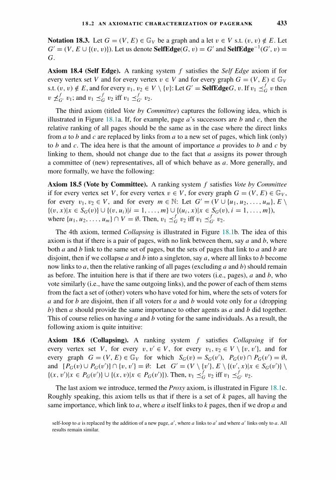
1 8 .2 an axiomatic characterization of pagerank 433
Notation 18.3. Let G = (V, E) ∈ GV be a graph and a let v ∈ V s.t. (v, v) /∈ E. LetG′ = (V, E ∪ {(v, v)}). Let us denote SelfEdge(G, v) = G′ and SelfEdge−1(G′, v) =G.
Axiom 18.4 (Self Edge). A ranking system f satisfies the Self Edge axiom if forevery vertex set V and for every vertex v ∈ V and for every graph G = (V, E) ∈ GV
s.t. (v, v) /∈ E, and for every v1, v2 ∈ V \ {v}: Let G′ = SelfEdgeG, v. If v1 /fG v then
v �/fG′ v1; and v1 /f
G v2 iff v1 /fG′ v2.
The third axiom (titled Vote by Committee) captures the following idea, which isillustrated in Figure 18.1a. If, for example, page a’s successors are b and c, then therelative ranking of all pages should be the same as in the case where the direct linksfrom a to b and c are replaced by links from a to a new set of pages, which link (only)to b and c. The idea here is that the amount of importance a provides to b and c bylinking to them, should not change due to the fact that a assigns its power througha committee of (new) representatives, all of which behave as a. More generally, andmore formally, we have the following:
Axiom 18.5 (Vote by Committee). A ranking system f satisfies Vote by Committeeif for every vertex set V , for every vertex v ∈ V , for every graph G = (V, E) ∈ GV ,for every v1, v2 ∈ V , and for every m ∈ N: Let G′ = (V ∪ {u1, u2, . . . , um}, E \{(v, x)|x ∈ SG(v)} ∪ {(v, ui)|i = 1, . . . , m} ∪ {(ui, x)|x ∈ SG(v), i = 1, . . . , m}),where {u1, u2, . . . , um} ∩ V = ∅. Then, v1 /f
G v2 iff v1 /fG′ v2.
The 4th axiom, termed Collapsing is illustrated in Figure 18.1b. The idea of thisaxiom is that if there is a pair of pages, with no link between them, say a and b, whereboth a and b link to the same set of pages, but the sets of pages that link to a and b aredisjoint, then if we collapse a and b into a singleton, say a, where all links to b becomenow links to a, then the relative ranking of all pages (excluding a and b) should remainas before. The intuition here is that if there are two voters (i.e., pages), a and b, whovote similarly (i.e., have the same outgoing links), and the power of each of them stemsfrom the fact a set of (other) voters who have voted for him, where the sets of voters fora and for b are disjoint, then if all voters for a and b would vote only for a (droppingb) then a should provide the same importance to other agents as a and b did together.This of course relies on having a and b voting for the same individuals. As a result, thefollowing axiom is quite intuitive:
Axiom 18.6 (Collapsing). A ranking system f satisfies Collapsing if forevery vertex set V , for every v, v′ ∈ V , for every v1, v2 ∈ V \ {v, v′}, and forevery graph G = (V, E) ∈ GV for which SG(v) = SG(v′), PG(v) ∩ PG(v′) = ∅,and [PG(v) ∪ PG(v′)] ∩ {v, v′} = ∅: Let G′ = (V \ {v′}, E \ {(v′, x)|x ∈ SG(v′)} \{(x, v′)|x ∈ PG(v′)} ∪ {(x, v)|x ∈ PG(v′)}). Then, v1 /f
G v2 iff v1 /fG′ v2.
The last axiom we introduce, termed the Proxy axiom, is illustrated in Figure 18.1c.Roughly speaking, this axiom tells us that if there is a set of k pages, all having thesame importance, which link to a, where a itself links to k pages, then if we drop a and
self-loop to a is replaced by the addition of a new page, a′, where a links to a′ and where a′ links only to a. Allresults remain similar.
434 1 8 the axiomatic approach and the internet
connect directly, and in a 1-1 fashion, the pages which linked to a to the pages that a
linked to, then the relative ranking of all pages (excluding a) should remain the same.This axiom captures equal distribution of importance. The importance of a is receivedfrom k pages, all with the same power, and is split among k pages; alternatively, thepages that link to a could pass directly the importance to pages that a link to, withoutusing a as a proxy for distribution. More formally, and more generally, we have thefollowing:
Axiom 18.7 (Proxy). A ranking system f satisfies Proxy if for every vertex set V ,for every vertex v ∈ V , for every v1, v2 ∈ V \ {v}, and for every graph G = (V, E) ∈GV for which |PG(v)| = |SG(v)|, for all p ∈ PG(v): SG(p) = {v}, and for all p, p′ ∈PG(v): p ∼f
G p′: Assume PG(v) = {p1, p2, . . . , pm} and SG(v) = {s1, s2, . . . , sm}. LetG′ = (V \ {v}, E \ {(x, v), (v, x)|x ∈ V } ∪ {(pi, si)|i ∈ {1, . . . , m}}). Then, v1 /f
G v2
iff v1 /fG′ v2.
18.2.4 A Representation Theorem for PageRank
Although we have provided some intuitive explanation for the axioms, one may arguethat particular axiom(s) are not that reasonable. As it turns out, however, all the pre-ceding axioms are satisfied by the PageRank procedure:
Proposition 18.8 (Altman and Tennenholtz, 2005). The PageRank ranking systemsatisfies isomorphism, self edge, vote by committee, collapsing, and proxy.
This proposition assures us of the soundness of the axioms. Moreover, it can beshown that the preceding axioms are not only satisfied by PageRank, but also completelyand uniquely characterize the PageRank procedure:
Theorem 18.9 (Altman and Tennenholtz, 2005). A ranking system f satisfies iso-morphism, self edge, vote by committee, collapsing, and proxy if and only if f is thePageRank ranking system.
The way this is shown, given Proposition 18.8, is by proving the uniqueness of thesystem satisfying the preceding axioms. Namely:
Proposition 18.10. Let f1 and f2 be ranking systems that satisfy isomorphism, selfedge, vote by committee, collapsing, and proxy. Then, f1 and f2 are the same rankingsystem (notation: f1 ≡ f2).
The proof in can therefore be viewed as “inefficient” procedure for computingPageRank. It starts from a graph which it slowly changes by application of the axioms.The sequence of graphs that are created maintain the ordering of a given pair of nodes,but get progressively “simpler.” In the end, the graph shrinks to only this single pairof nodes, where the ordering of PageRank is determined by the number of their selfloops. Technically, the axioms are not used directly to derive all of the graphs in thesequence. Instead, the transitions between graphs are based on higher level propertiesderived from the axioms (the complete definition of these properties and their use isquite lengthy).
1 8 .3 trust-based recommendations 435
An interesting open problem is whether the preceding axioms are independent. Thecurrent conjecture, offered by Altman and Tennenholtz (2005), is that they are.
18.3 Trust-Based Recommendations
Reputation, recommendation, and trust systems have become fundamental and essentialingredients of multiagent systems, especially in e-commerce applications (e.g., Klein-berg, 1999; Resnick et al., 2000; Bakos and Dellarocas, 2003; Tennenholtz, 2004;Dash et al., 2004). All of these systems aggregate agents’ reviews of one another, aswell as about external events, into valuable information. Notable commercial exam-ples include Amazon and E-Bay’s recommendation and reputation systems (Resnickand Zeckhauser, 2001), and the Epinions web of trust/reputation system (Massa andAvesani, 2005). Personalized recommendations add value to an agent’s experience andmay also be naturally paired with personalized advertising.
In a typical application, there is an item of interest (e.g., a product, service, candidate,restaurant). A subset of the agents have prior opinions about this item. Any of theremaining agents might want to estimate whether they would like the item or not,based on the opinions of others. In the real world, a person might first consult friendsfor their recommendations. In turn, the friends (who do not have opinions of theirown) may consult their friends, and so on. Based on the cumulative feedback thatis received, an agent might form its own subjective opinion. An automated trust-based recommendation system aims to simulate such a process to provide high-qualitypersonalized recommendations to agents.
The model we present here (which was originally presented by Andersen et al.,2008) represents the social connections using a directed graph, partially labeled with ±votes. A node in the graph represents an agent, an edge from a to b represents thefact that agent a trusts agent b, and a subset of the nodes are labeled by + or −,indicating prior opinions. Based on this input, the recommendation system must outputa recommendation for each unlabeled node. We call such an abstraction a voting networkbecause it models a variety of two-candidate voting systems, where the candidatesare + and −.
We first show that a number of elementary axioms lead to an impossibility theorem.This set is minimal in the sense that any proper subset of the axioms is satisfiedby some recommendation system. We then explore relaxations that lead to a uniquesystem that is most easily described in terms of random walks. Then we show a secondaxiomatization that leads to a unique “min-cut” system on graphs. For simplicity, thefocus is placed on the case of unweighted graphs and binary votes.
18.3.1 Notation and Definitions
We now formally define the basic setting of a trust-based recommendation system.
Definition 18.7. A voting network is a directed annotated multigraph G =(N, V+, V−, E) where N is a set of nodes, V+, V− ⊆ N are disjoint subsets of positiveand negative voters, and E ⊆ N2 is a multiset of edges with parallel edges allowed butno self loops.

436 1 8 the axiomatic approach and the internet
Edges in the voting network imply trust relations between participants, and multipleparallel edges, signify a stronger degree of trust. When V+ and V− are clear fromcontext, we denote the set of voters by V = V+ ∪ V− and the set of nonvoters byV = N \ V .
Definition 18.8. A recommendation system R takes as input a voting network G andsource s ∈ V and outputs recommendation R(G, s) ∈ {−, 0,+}. We denote R(G) =〈R+(G), R−(G), R0(G)〉 where R+(G) = {s ∈ V | R(G, s) = +} and similarly forR−(G), R0(G).
We denote by sgn : R → {−, 0,+} the function that computes the sign of its input.We denote by PredE(v) and SuccE(v) the multisets of nodes that point to v and that v
points to, respectively.Given a multiset of recommendations, S ⊆ {−, 0,+}, we define the majority
MAJ(S) to be + if a strict majority of S is +, − if a strict majority of S is −,and 0 otherwise (a strict majority simply means more than half).
18.3.2 Five Appealing Properties and an Impossibility
We now consider various properties of recommendation systems as candidate axioms.The first property, Symmetry, is purely structural. Symmetry implies that the namesof the agents do not matter for the source node; all that matters is the structure of thetrust graph and the votes provided. In addition we treat the values +/- as arbitrary, andrequire that they be treated symmetrically.
Axiom 18.11 (Symmetry). A recommendation system R satisfies Anonymity if forevery voting network G = (N, V+, V−, E): For any permutation π : N → N , let G′,be the isomorphic voting network under π . Then R+(G′) = π(R+(G)) and R−(G′) =π(R−(G)).
A recommendation system R satisfies Neutrality if for every voting network G =(N, V+, V−, E): Let G′′ = (N, V−, V+, E). Then R+(G) = R−(G′′) and R−(G) =R+(G′′).
A recommendation system R satisfies Symmetry if it satisfies both Anonymity andNeutrality.
The next axiom states that if a node s has recommendation 0 (or +) and a brand new+-voter is added to the network along with an edge from s to the new node, then s’s newrecommendation should be +. It reflects a razor’s-edge view of a 0 recommendation.The axiom “pushes” the systems toward strict recommendations. (Without such anaxiom, systems may almost always recommend 0.)
Axiom 18.12 (Positive Response). A recommendation system R satisfies PositiveResponse if for every voting network G = (N, V+, V−, E): for every w �∈ N , s ∈ V ,and G′ = (N ∪ {w}, V+ ∪ {w}, V−, E 0 {(s, w)}); If s /∈ R−(G) then s ∈ R+(G′).
Note that this axiom is presented asymmetrically in terms of ± votes and recommen-dations. In combination with the Symmetry axiom, the corresponding version with −votes and recommendations follows directly. We use an asymmetric presentation forreadability in several of the axioms.
1 8 .3 trust-based recommendations 437
The next axiom, Independence of Irrelevant Stuff (IIS), captures the fact that votershave already made up their minds. This means that when considering the recommenda-tion for a particular source node in a particular trust graph, where part of the agents vote(perhaps based on first-hand experience), feedback from these agents is independent ofwho they trust (i.e., they trust themselves infinitely more than others) and the recom-mendation system should consider only reachable nodes and should ignore links out ofvoters. While one may consider other types of semantics, this one is (approximately)quite typical for actual systems.
Axiom 18.13 (IIS). A recommendation system R satisfies Independence of IrrelevantStuff (IIS) if for every voting network G = (N, V+, V−, E): for any edge e ∈ V × N
leaving a voter, and the subgraph G′ = (N, V+, V−, E \ {e}) in which e has beenremoved, R(G) = R(G′). In addition, for every s ∈ V and v ∈ N not reachable froms, for the subgraph G′′ in which node v (and its associated edges) have been removed,we have R(G, s) = R(G′′, s).
When we write R(G) = R(G′), as earlier, the recommendations in the two votingnetworks are identical.
Notice that IIS captures two aspects of relevant information. First, when one expe-riences a service, trust relations are irrelevant, as his opinion is completely framed byhis direct experience; second, the opinion of a person unreachable in the trust networkis irrelevant.
The following requirement deals with some minimal rationality we wish to attributeto the agents; as in the classical theory of choice we are willing to assume somethingabout the vote of an agent who has no a priori opinion only in extreme cases. TheNeighborhood Consensus axiom does just that: if all the outgoing neighbors of (i.e.,agents trusted by) a node v in a trust network vote +, and no other nodes point to v’sneighbors, then v might be considered to vote + as well. Formally, we have:
Axiom 18.14 (Neighborhood Consensus). A recommendation system R satisfiesNeighborhood Consensus if for every voting network G = (N, V+, V−, E), and forevery distinct nonvoters s, u ∈ V , where u has at least one outgoing edge and eachoutgoing edge (u, v) ∈ E points to v such that v ∈ V+ and v has no (incoming oroutgoing) neighbors other than u: Let G′ = (N, V+ ∪ {u}, V−, E), then R(G, s) =R(G′, s).
Transitivity is a central concept in the axiomatization of voting, and in our intuitionregarding trust relations. In this context, we consider the case when the underlyingtrust graph is fixed, while the system needs to deal with more than one item, wheredifferent subsets of nodes vote on different items. The idea is that if a source node isrecommended, say, +, then it means that the system assigns higher trust to the agentswho report + than to the agents who report −.
Definition 18.9. Let G = (N, V+, V−, E) be a voting network , s ∈ V , and R a rec-ommendation system. If s ∈ R+(G), then we say that s trusts V+ more than V− relativeto multigraph (N, E) under the recommendation system R.
438 1 8 the axiomatic approach and the internet
In this case, a partial ordering among sets of nodes is generated, and we wish thisrelation to be transitive. This axiom is not only natural, but also builds a strong tiebetween trust systems and recommendation systems.
Axiom 18.15 (Transitivity). A recommendation system R satisfies Transitivity if forall multigraphs (N, E), and mutually disjoint A, B, C ⊆ N , and s /∈ A ∪ B ∪ C: if s
trusts A more than B and s trusts B more than C, then s trusts A more than C.
Unfortunately, the following result, says that the five axioms cannot be obtainedsimultaneously by any system.
Theorem 18.16 (Andersen et al., 2008). The axioms Symmetry, Positive Response,Independence of Irrelevant Stuff (IIS), Neighborhood Consensus, and Transitivity areinconsistent. Any proper subset of these axioms is satisfied by some reputation system.
18.3.3 Alternatives to Transitivity and the Random Walk System
In this section, we consider propagation of trust. Intuitively, if u trusts v and v trustsw, then u trusts w as well. Much has been written about trust propagation withinsocial networks (see, e.g., Guha et al., 2004) and the following axiom is a conservativeinterpretation that agrees with much of the literature.
One would like to say that if u trusts nonvoter v, and v trusts w, then we can simplyadd an edge from u to w without changing anything. However, the system is supposedto reflect degrees of trust, and this would falsely inflate such trust. Instead, edges arecounted as follows. Suppose there are k edges leaving v (that do not point to u). Supposethat there happen to be k edges from u to v. Then we can remove k edges from u to v
and replace them by k new edges from u to the k nodes that v trusts (besides u), andno recommendations should change.
Axiom 18.17 (Trust Propagation). A recommendation system R satisfies TrustPropagation if for every voting network G = (N, V+, V−, E): for every distinctu, v ∈ V , suppose that the edges leaving v (besides those to u) are (v, w1), . . . , (v, wk),(wi �= u) for some integer k, and that E contains exactly k copies of (u, v). Then, forE′ = (
E 0 {(u, w1), . . . , (u, wk)}) \ {(u, v) ∗ k} and G′ = (N, V+, V−, E′), we havethat R(G) = R(G′).
Another natural axiom is Scale Invariance. Loosely speaking, this means that theamount of trust placed in a node is relative.
Axiom 18.18 (Scale Invariance). A recommendation system R satisfies Scale Invari-ance if for every voting network G = (N, V+, V−, E): for every u ∈ V , and k � 1, letG′ = (N, V+, V−, E 0 E′), where E′ is the multiset containing k copies of each of theedges leaving u, then R(G) = R(G′).
It states that we can duplicate all edges leaving a node an arbitrary number of timeswithout changing recommendations.
Theorem 18.19. Axioms Symmetry, Positive Response, Independence of IrrelevantStuff (IIS), Neighborhood Consensus, Trust Propagation and Scale Invariance aresatisfied uniquely by the Random Walk System (see later).
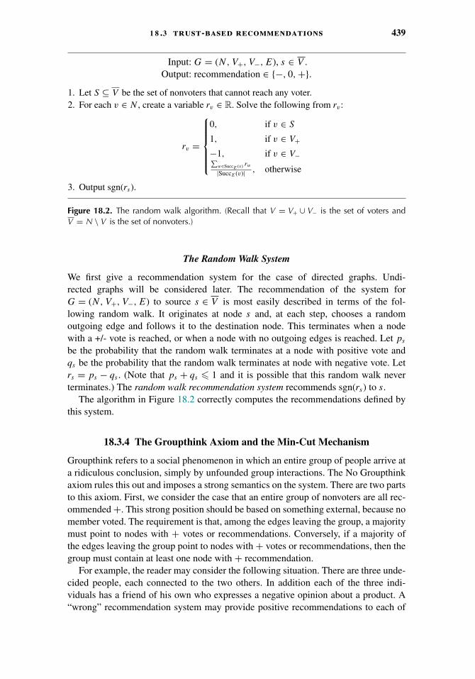
1 8 .3 trust-based recommendations 439
Input: G = (N, V+, V−, E), s ∈ V .Output: recommendation ∈ {−, 0,+}.
1. Let S ⊆ V be the set of nonvoters that cannot reach any voter.2. For each v ∈ N , create a variable rv ∈ R. Solve the following from rv:
rv =
⎧⎪⎪⎪⎪⎨⎪⎪⎪⎪⎩0, if v ∈ S
1, if v ∈ V+−1, if v ∈ V−∑
w∈SuccE (v) rw
|SuccE (v)| , otherwise
3. Output sgn(rs).
Figure 18.2. The random walk algorithm. (Recall that V = V+ ∪ V− is the set of voters andV = N \ V is the set of nonvoters.)
The Random Walk System
We first give a recommendation system for the case of directed graphs. Undi-rected graphs will be considered later. The recommendation of the system forG = (N, V+, V−, E) to source s ∈ V is most easily described in terms of the fol-lowing random walk. It originates at node s and, at each step, chooses a randomoutgoing edge and follows it to the destination node. This terminates when a nodewith a +/- vote is reached, or when a node with no outgoing edges is reached. Let ps
be the probability that the random walk terminates at a node with positive vote andqs be the probability that the random walk terminates at node with negative vote. Letrs = ps − qs . (Note that ps + qs � 1 and it is possible that this random walk neverterminates.) The random walk recommendation system recommends sgn(rs) to s.
The algorithm in Figure 18.2 correctly computes the recommendations defined bythis system.
18.3.4 The Groupthink Axiom and the Min-Cut Mechanism
Groupthink refers to a social phenomenon in which an entire group of people arrive ata ridiculous conclusion, simply by unfounded group interactions. The No Groupthinkaxiom rules this out and imposes a strong semantics on the system. There are two partsto this axiom. First, we consider the case that an entire group of nonvoters are all rec-ommended +. This strong position should be based on something external, because nomember voted. The requirement is that, among the edges leaving the group, a majoritymust point to nodes with + votes or recommendations. Conversely, if a majority ofthe edges leaving the group point to nodes with + votes or recommendations, then thegroup must contain at least one node with + recommendation.
For example, the reader may consider the following situation. There are three unde-cided people, each connected to the two others. In addition each of the three indi-viduals has a friend of his own who expresses a negative opinion about a product. A“wrong” recommendation system may provide positive recommendations to each of
440 1 8 the axiomatic approach and the internet
the undecided persons, saying that now each one of them is consistent with themajority of his friends. This is a typical example of group thinking that we wish toavoid.
Formally, we say that a recommendation system R avoids Groupthink for G =(N, V+, V−, E) if the following holds.
Axiom 18.20 (No Groupthink). A recommendation system R satisfies No Group-think if for every voting network G = (N, V+, V−, E), and S ⊆ V , a nonemptyset of nonvoters: Let E′ be the multiset of edges in E from S to N \ S. (a) IfS ⊆ R+(G) (resp. R−(G)), then a strict majority of the edges in E′ must point tonodes in R+(G) ∪ V+ (resp. R−(G) ∪ V−). (b) Conversely, if a strict majority of theedges in E′ point to nodes in R+(G) ∪ V+ (resp. R−(G) ∪ V−), then S ∩ R+(G) �= ∅(resp. S ∩ R−(G) �= ∅).
As it turns out, the No Groupthink axiom can not be satisfied in general directedgraphs. We define it here for specific graphs, namely, undirected graphs, as the onesemployed, for example, by Facebook. An undirected graph is a (directed) graph wherenode v links to node u iff node u links to node v.
Theorem 18.21. Axiom No Groupthink on an undirected graph implies the min-cutrecommendation system (see later).
The Min-Cut System
Let G = (N, V+, V−, E) be a voting network. Let E′ ⊆ E be the set of edges in E thatoriginate at nonvoters, that is, eliminate edges out of voters. We say that cut C ⊆ E′ isa V+-V− cut of G if there is no path from V+ to V− using edges in E′ \ C. We say thatC is a min cut of G if its size |C| is minimal among all such cuts.
More intuitively, a cut in a voting network is a set of the edges, originating fromnonvoters, such that any path from a + voter to a − voter must pass through at leastone of them. A min-cut is such a cut of minimal size.
The min-cut system can be defined as follows. The recommendation of a source s is+ (resp. −) if and only if in all min-cuts there is a path from s to V+ (resp. V−) amongedges in E′ \ C. If neither is the case, then the recommendation is 0.
This is easily computed as follows. Compute a min-cut C. Then, consider the graphwhen adding an edge from source s to a + (resp. −) voter and compute C+ (resp. C−).If |C| < |C−| then the recommendation is +. If |C| < |C+| then the recommendationis −. Otherwise, the recommendation is 0. The computation can be done efficientlybecause min s-t cut can be found in polynomial time. To see that this procedure matchesthe preceding definition, note that if s is connected to V+ in all min-cuts then adding anedge from s to a − voter will create a path from V− to V+ in any min-cut and necessarilyincrease the min-cut cost by 1. Similarly if s is connected to V− in all min-cuts. Inthe remaining case, the sizes of all three min-cuts will be the same because there aresome min-cuts in which s is not connected to V− and some in which s is not connectedto V+.
1 8 .4 mechanisms for multilevel marketing 441
18.4 Mechanisms for Multilevel Marketing
Social networks have existed long before the Internet, but their recent web-based form,as exhibited by companies like Facebook, Twitter, or LinkedIn, made them more tan-gible. In this new manifestation, social networks have become an attractive playgroundfor viral marketing: the dream of any marketer is to successfully market products via“word of mouth” thus utilizing social networks. In order to make that dream a reality,various forms of marketing have been advocated. The so-called affiliate marketing,direct marketing, and multilevel marketing all refer to (overlapping) approaches thatfacilitate viral marketing.
The fundamental idea behind multilevel marketing is that one customer, who alreadypurchased the product, is rewarded for referrals, that is, for purchases made by anotheras a result of his promotion. The reward mechanism associated with multi-level market-ing may take various forms. In particular, agents may be rewarded for both purchasesmade by direct referrals and for indirect ones in a recursive manner.
The potential to accumulate small rewards from each person to a sizable sum, afeature which is now manageable thanks to the Internet and information technology, isimportant as it allows advertisers to attract early adopters and trendsetters that are ofgreat value to them. (On the downside, the possibility of gathering a large sum has alsoinspired more illicit versions of multilevel marketing, which are not really intendedto promote a product, namely, pyramid schemes.) Needless to say that selecting anappropriate reward mechanism is inherent to the design of a successful multilevelmarketing scheme.
The design of mechanisms for social settings is widely relevant. Kleinberg andRaghavan (2005) consider a setting that is perhaps the most similar in spirit to theone presented here, in which they elicit effort from agents that forward queries in asocial network. In their setting, the final rewards are only allocated along the pathto the agent that gave the answer, and not to all those who forwarded the question.Similar reward mechanisms were used by the team from MIT that won the DARPAnetwork challenge (Pickard et al., 2011), in the context of incremental deployment onthe Internet (Douceur and Moscibroda, 2007), and in the context of message passingwithin the Bitcoin protocol (Babaioff et al., 2012).
18.4.1 The Referral Tree Model
There are many possible ways to take the social network that forms the basis of thereferral process into account. In principle, one may wish to consider the times atwhich promoting messages were sent from one user to another, to consider referralsthat were not followed up by a purchase of the product being promoted, or even toconsider the social links along which a referral was not made. However, this informationmay not be all available to the original seller.5 We therefore take the straightforward
5 In some social networks such as Facebook there is often more explicit knowledge of social connections, butgeneral referral systems do not necessarily have all the information about the underlying social structure andmay not be able to track messages in the network.

442 1 8 the axiomatic approach and the internet
approach of looking only at the structure of successful referrals. For each buyer, wemark only a single referrer for introducing the product to her (in reality, this wouldtypically be specified at the time of purchase). The induced structure of referrals formsa collection of directed trees, each rooted at a node that corresponds to some buyer thathas purchased the product directly from the seller.
To better illustrate why trees (and more generally forests) are considered, picturethe following tracking procedure for Internet affiliate marketing: Upon purchasing aproduct the buyer gets a code; this code can be now shared by him/her in any way(SMS, email, Facebook page, etc.); when another user makes a purchase and providesthat code, this fact is recorded. The original owner of the code may then get somereward for a successful referral. The new buyer then gets another code, which may beused further. Notice that a code is delivered only upon purchase, and a buyer showsa particular code (associated with another buyer) upon purchase following a referral.This creates a well-define forest structure which will be used to allocate the rewards.
We shall refer to this tree collection as the referrals forest, denoted T , and to therooted trees in T as the referrals trees. We find the assumption that T can be maintainedby the seller sufficiently weak.
It should be clarified that the referrals forest corresponds to a single multilevelmarketing campaign (typically associated with a single product). Moreover, socialnetwork users that did not purchase the product are not represented in T even if someof their friends have sent them referrals. For ease of presentation, we assume that Tis fully known when the rewards are to be distributed, although all the mechanismsexplored in this section are also suited for incremental payments performed online. Itwill also be convenient to identify the buyers with their corresponding nodes in T ,denoting the reward of (the buyer corresponding to) node u under the referrals forestT by RT (u).
18.4.2 Properties of Reward Mechanisms
The reward mechanism is essentially a function that maps the referrals forest T tothe nonnegative real rewards of its nodes. However, not every such function shouldbe considered; specifically, we impose three constraints on the reward mechanisms.Through the remainder of the chapter, these axioms will not be questioned, but willrather be considered a part of every reward mechanism. The first one is the Subtreeconstraint:
Axiom 18.22 (SubTree (ST)). A reward mechanism R satisfies the Subtree axiom if:RT (u) is uniquely determined by Tu, namely, by the subtree of T rooted at u.
This is sensible, as each user u can really be credited only for bringing in users shepromoted the product to, either directly (the children of u in T ) or indirectly (lowerlevel descendants of u). Moreover, a dependence of RT (u) on the position of u withinT (rather than on Tu only) may result in an undesirable behavior on behalf of u: insome cases u is better off delaying the purchase of the product after receiving a referralin hope for a “better” offer, that is, for a referral that would place u in a better positionwithin T .

1 8 .4 mechanisms for multilevel marketing 443
One of the consequences of the subtree constraint is that there is no point in dealingwith the referrals forest T in full, but rather focus on trees which are rooted at thenodes whose reward we are trying to calculate. In other words, the reward mechanism iscompletely specified by the function R(T ) that maps the rooted tree T to the nonnegativereal reward of its root (which may be an internal node within the whole referrals forest).
The second constraint that we impose on the reward mechanism is the Budgetconstraint: the seller is willing to spend at most a certain fraction φ � 1 of her totalincome on rewarding her buyers for referrals. Given that the price of the product isπ , this means that the total sum of rewards given to all nodes is at most φ · π |T |. Weassume without loss of generality that π and φ are scaled so that φ · π = 1. Thus,
Axiom 18.23 (Budget Constraint (BC)). A reward mechanism R satisfies the BudgetConstraint if: ∑
u∈TR(Tu) � |T | .
The third requirement is the Unbounded Reward constraint: there is no limit to therewards one can potentially receive even under the assumption that each user has alimited circle of friends in the underlying social network (imposing a limited numberof direct referrals). This requirement is a way to capture the high motivation that isgiven in affiliate marketing schemes even to those with a bounded number of friends.Formally,
Axiom 18.24 (Unbounded Reward (UR)). A reward mechanism R satisfiesUnbounded Reward if: there exists some positive integer d (a property of the rewardmechanism) such that for every real Rθ , there exists some tree T of maximum degreed (i.e., every node has at most d children) such that R(T ) � Rθ .
In particular, this constraint implies that the reward mechanisms we consider musttake indirect referrals into account. From this point on, we restrict discussion only tomechanisms for which the three preceding axioms (ST, BC, UR) hold. We term theseproper reward mechanisms.
18.4.3 Geometric Mechanisms
We now focus on characterizing the following well-known family of reward mecha-nisms, referred to as geometric mechanisms. Given two constants 0 < a < 1 and b > 0such that b + 1 � 1/a, the reward from a referral tree T under the (a, b)-geometricmechanism is defined to be
R(T ) =∑u∈T
adep(u) · b .
Where dep(u) is the depth of node u in the referral tree. The constraints on a and b
ensure that the amount contributed by each node to the reward of its ancestors will notexceed 1.
Let us begin by defining and discussing three additional properties (that will proveuseful in the context of geometric mechanisms). We define the operation ∪ on trees

444 1 8 the axiomatic approach and the internet
such that if T1, T2 are trees, then T1 ∪ T2 is the tree formed by contracting (or merging)the roots of T1 and T2. This allows us to define the Additivity axiom as follows:
Axiom 18.25 (Additivity (ADD)). A reward mechanism R satisfies Additivity if: forany two disjoint trees T , T ′
R(T ) + R(T ′) = R(T ∪ T ′).
This property suggests that if two disjoint trees are merged at the root, then thereward of the root is exactly the sum of the rewards of the two original trees. Generallyspeaking this property implies that the reward to each node can be independentlyattributed to the subtrees rooted at its children.
The next axiom, Child Dependence, determines the reward of the root uniquely fromthe rewards of its children. This property ensures that the actual computation of therewards can be performed locally. In fact, we shall consider a weaker condition for thisproperty:
Axiom 18.26 (Child Dependence (CD)). A reward mechanism R satisfies Child Depen-dence if: given that the root of T has a single child u, then R(T ) is uniquely determinedby R(Tu).
This is captured by a function χ : R�0 → R�0 (a property of the mechanism) sothat R(T ) = χ(R(Tu)).
The next axiom states that the reward R(T ) is uniquely determined by the numberof nodes on each depth level in T . We denote by dk the number of nodes of T at depthlevel k > 0, and the infinite vector containing these numbers for all depth levels byd = (d1, . . . , dh, 0, 0, . . . ), where h is the height of the tree. Let D be the set of all suchvectors, that is, the set of all infinite vectors over Z�0 with a strictly positive prefixfollowed by a countably infinite suffix of zeros.
Axiom 18.27 (Depth Level Dependence (DLD)). A reward mechanism R satisfiesDepth Level Dependence if: There exists some function f : D → R�0 (a property ofthe mechanism) such that R(T ) = f (d).
This property essentially means that the credit for a referral depends solely on howdirect (or better said, indirect) this referral is.
The preceding axioms characterize the family of geometric mechanisms:
Theorem 18.28 (Emek et al., 2011). A proper reward mechanism satisfies DLD, ADD,and CD if and only if it is a geometric mechanism.
An appealing property of geometric mechanisms is that the contribution of descen-dants to their ancestor decreases with distance. This reflects the fact that the ancestorgets less credit for more distant indirect referrals.
It is important to point out that each of the three properties we used to characterizethe family of geometric mechanisms is needed, that is, if we remove one of the threeproperties then there exists another proper mechanism (outside the geometric family)for which the remaining two hold.
To prove the theorem, we will need the definition of the following additionalproperty:
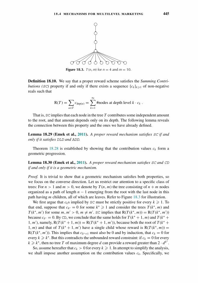
1 8 .4 mechanisms for multilevel marketing 445
Figure 18.3. T (n, m) for n = 4 and m = 10.
Definition 18.10. We say that a proper reward scheme satisfies the Summing Contri-butions (SC) property if and only if there exists a sequence {ck}k�1 of non-negativereals such that
R(T ) =∑u∈T
cdep(u) =∞∑
k=1
#nodes at depth level k · ck .
That is,SC implies that each node in the tree T contributes some independent amountto the root, and that amount depends only on its depth. The following lemma revealsthe connection between this property and the ones we have already defined.
Lemma 18.29 (Emek et al., 2011). A proper reward mechanism satisfies SC if andonly if it satisfies DLD and ADD.
Theorem 18.28 is established by showing that the contribution values ck form ageometric progression.
Lemma 18.30 (Emek et al., 2011). A proper reward mechanism satisfies SC and CDif and only if it is a geometric mechanism.
Proof. It is trivial to show that a geometric mechanism satisfies both properties, sowe focus on the converse direction. Let us restrict our attention to a specific class oftrees: For n > 1 and m > 0, we denote by T (n, m) the tree consisting of n + m nodesorganized as a path of length n − 1 emerging from the root with the last node in thispath having m children, all of which are leaves. Refer to Figure 18.3 for illustration.
We first argue that cks implied by SC must be strictly positive for every k � 1. Tothat end, suppose that ck∗ = 0 for some k∗ � 1 and consider the trees T (k∗, m) andT (k∗, m′) for some m, m′ > 0, m �= m′. SC implies that R(T (k∗, m)) = R(T (k∗, m′))because ck∗ = 0. By CD, we conclude that the same holds for T (k∗ + 1, m) and T (k∗ +1, m′), namely, R(T (k∗ + 1, m)) = R(T (k∗ + 1, m′)), because both the root of T (k∗ +1, m) and that of T (k∗ + 1, m′) have a single child whose reward is R(T (k∗, m)) =R(T (k∗, m′)). This implies that ck∗+1 must also be 0 and by induction, that ck = 0 forevery k � k∗. But this contradicts the unbounded reward constraint: if ck = 0 for everyk � k∗, then no tree T of maximum degree d can provide a reward greater than 2 · dk∗
.So, assume hereafter that ck > 0 for every k � 1. In attempt to simplify the analysis,
we shall impose another assumption on the contribution values ck . Specifically, we
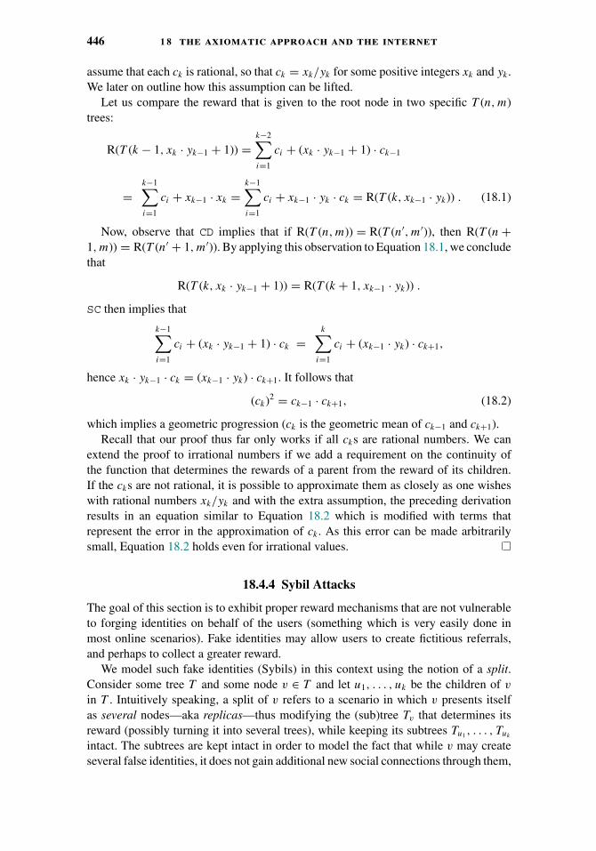
446 1 8 the axiomatic approach and the internet
assume that each ck is rational, so that ck = xk/yk for some positive integers xk and yk .We later on outline how this assumption can be lifted.
Let us compare the reward that is given to the root node in two specific T (n, m)trees:
R(T (k − 1, xk · yk−1 + 1)) =k−2∑i=1
ci + (xk · yk−1 + 1) · ck−1
=k−1∑i=1
ci + xk−1 · xk =k−1∑i=1
ci + xk−1 · yk · ck = R(T (k, xk−1 · yk)) . (18.1)
Now, observe that CD implies that if R(T (n, m)) = R(T (n′, m′)), then R(T (n +1, m)) = R(T (n′ + 1, m′)). By applying this observation to Equation 18.1, we concludethat
R(T (k, xk · yk−1 + 1)) = R(T (k + 1, xk−1 · yk)) .
SC then implies that
k−1∑i=1
ci + (xk · yk−1 + 1) · ck =k∑
i=1
ci + (xk−1 · yk) · ck+1,
hence xk · yk−1 · ck = (xk−1 · yk) · ck+1. It follows that
(ck)2 = ck−1 · ck+1, (18.2)
which implies a geometric progression (ck is the geometric mean of ck−1 and ck+1).Recall that our proof thus far only works if all cks are rational numbers. We can
extend the proof to irrational numbers if we add a requirement on the continuity ofthe function that determines the rewards of a parent from the reward of its children.If the cks are not rational, it is possible to approximate them as closely as one wisheswith rational numbers xk/yk and with the extra assumption, the preceding derivationresults in an equation similar to Equation 18.2 which is modified with terms thatrepresent the error in the approximation of ck . As this error can be made arbitrarilysmall, Equation 18.2 holds even for irrational values.
18.4.4 Sybil Attacks
The goal of this section is to exhibit proper reward mechanisms that are not vulnerableto forging identities on behalf of the users (something which is very easily done inmost online scenarios). Fake identities may allow users to create fictitious referrals,and perhaps to collect a greater reward.
We model such fake identities (Sybils) in this context using the notion of a split.Consider some tree T and some node v ∈ T and let u1, . . . , uk be the children of v
in T . Intuitively speaking, a split of v refers to a scenario in which v presents itselfas several nodes—aka replicas—thus modifying the (sub)tree Tv that determines itsreward (possibly turning it into several trees), while keeping its subtrees Tu1, . . . , Tuk
intact. The subtrees are kept intact in order to model the fact that while v may createseveral false identities, it does not gain additional new social connections through them,
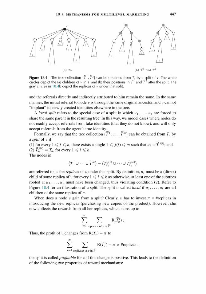
1 8 .4 mechanisms for multilevel marketing 447
v
2
4
5
6
7
1
3
8
(a) Tv
1
2
3
4
6
5
7
8
(b) T 1 and T 2
Figure 18.4. The tree collection {T 1, T 2} can be obtained from Tv by a split of v. The whitecircles depict the (a) children of v in T and (b) their positions in T 1 and T 2 after the split. Thegray circles in 18.4b depict the replicas of v under that split.
and the referrals directly and indirectly attributed to him remain the same. In the samemanner, the initial referral to node v is through the same original ancestor, and v cannot“implant” its newly created identities elsewhere in the tree.
A local split refers to the special case of a split in which u1, . . . , uk are forced toshare the same parent in the resulting tree. In this way, we model cases where nodes donot readily accept referrals from fake identities (that they do not know), and will onlyaccept referrals from the agent’s true identity.
Formally, we say that the tree collection {T 1, . . . , T m} can be obtained from Tv bya split of v if(1) for every 1 � i � k, there exists a single 1 � j (i) � m such that ui ∈ T j (i); and(2) T
j (i)ui
= Tuifor every 1 � i � k.
The nodes in (T 1 ∪ · · · ∪ T m
)− (T j (1)
u1∪ · · · ∪ T j (k)
uk
)are referred to as the replicas of v under that split. By definition, ui must be a (direct)child of some replica of v for every 1 � i � k as otherwise, at least one of the subtreesrooted at u1, . . . , uk must have been changed, thus violating condition (2). Refer toFigure 18.4 for an illustration of a split. The split is called local if u1, . . . , uk are allchildren of the same replica of v.
When does a node v gain from a split? Clearly, v has to invest π × #replicas inintroducing the new replicas (purchasing new copies of the product). However, shenow collects the rewards from all her replicas, which sums up to
m∑i=1
∑replica u of v in T i
R(T iu ) .
Thus, the profit of v changes from R(Tv) − π to
m∑i=1
∑replica u of v in T i
R(T iu ) − π × #replicas ;
the split is called profitable for v if this change is positive. This leads to the definitionof the following two properties of reward mechanisms:
448 1 8 the axiomatic approach and the internet
Axiom 18.31 (Split Proof (SP)). A reward mechanism R is Split Proof if it does notadmit a profitable split for any node v in any tree T .
Axiom 18.32 (Local Split Proof (LSP)). A reward mechanism R is Local Split Proofif it does not admit a profitable local split for any node v in any tree T .
The geometric mechanisms presented in Section 18.4.3 do not satisfy SP. In fact,they do not even satisfy LSP (see Section 18.4.5). A simple mechanism that doessatisfy SP is the single level mechanism defined by fixing RMsl (T ) = α · deg(r) forsome constant α � 1, however, this mechanism does not adhere to the UnboundedReward constraint.
18.4.5 Negative Results
Let us now exhibit two negative results regarding the design of split-proof mechanisms.The first result shows that the reward guaranteed to a node in a split-proof mechanismcannot be a constant fraction of even its least influential child.
Lemma 18.33 (Emek et al., 2011). A proper reward mechanism that satisfies LSPcannot guarantee a node some fraction 0 < α � 1 of the reward of its least rewardedchild.
Next, we see that even a family of reward mechanisms much wider than geometricmechanisms is still not split-proof. This requires the introduction of another axiomwhich is clearly satisfied by every geometric mechanism (thus, it is not independent),yet, cannot replace any of the characterizing properties listed in Theorem 18.28.
Axiom 18.34 (Monotonicity (MONO)). A reward mechanism R satisfies Monotonicityif: for every pair of trees T , T ′ such that the tree T can be obtained from the tree T ′ byremoving some leaf, then R(T ) < R(T ′).
Lemma 18.35 (Emek et al., 2011). A proper reward mechanism that satisfies MONOand ADD cannot satisfy SP.
18.4.6 A Split-Proof Mechanism
In this section we present a split-proof reward mechanism, denoted Msplit. Informally,the mechanism Msplit is defined in two stages: in the first stage, we define a simplebase mechanism, denoted Mbase; Msplit is then defined with respect to the maximumprofit a node can make under Mbase from splits.
Mechanism Mbase
The base mechanismMbase is defined by setting RMbase (T ) to be the maximum h ∈ Z�0
such that T exhibits as a subtree, a perfect binary tree6 B rooted at r whose height ish. In that case we say that B realizes RMbase (T ) (see Figure 18.5). If there are several
6 A perfect binary tree is a rooted tree in which all leaves are at the same distance from the root and all nonleaveshave exactly two children.

1 8 .4 mechanisms for multilevel marketing 449
Figure 18.5. The tree T and the perfect binary tree that realizes RMbase (T ) (nodes depicted bygray circles).
perfect binary trees that can realize RMbase (T ), then it will be convenient to take thefirst one in a lexicographic order based on a breadth-first-search traversal and considerit as the perfect binary tree that realizes RMbase (T ).
A node u ∈ T is said to be visible in T if it belongs to the perfect binary tree thatrealizes RMbase (T ); otherwise, u is said to be invisible in T . This definition is extendedas follows: given some ancestor v of u in T , u is said to be visible to v if u is visiblein Tv , and invisible otherwise. The parent of a (nonroot) node u in T is denoted pT (u).Note that if u is invisible to v, then it is also invisible to pT (v) (assuming of coursethat v �= r). The contrary is not necessarily true: u may be visible to v but invisibleto pT (v). By definition, for every node u ∈ T and for every j ∈ Z�1, it holds that u
admits either 2j or 0 visible depth-j descendants.We denote the distance from u to v by δT (u, v), that is, the number of edges along
the unique path in T leading from u to v. The mechanism Mbase can now be redefinedby setting
RMbase (T ) =∑
visible u∈T
2−δT (u,r) .
This alternative view of mechanism Mbase calls for the definition of contributions: anode u ∈ T contributes 2−k to the reward of its kth ancestor v, k � 1, if u is visible tov; otherwise, u does not contribute anything to the reward of v. Let CMbase (u, v) denotethe contribution of u to the reward of v under Mbase. The reward of a node can now becalculated by summing the contributions that its descendants make to it. This impliesthat Mbase satisfies the budget constraint: the total contribution made by a node u ∈ T
to all its ancestors is bounded from above by the geometric sum∑δ(u,r)
j=1 2−j < 1, hence,by changing the summation, we conclude that
∑v∈T RMbase (Tv) < |T |.
Mechanism Msplit
The mechanism Msplit is defined by setting RMsplit (T ) so that it reflects the maximumprofit that r can get under Mbase from splits. More formally, let S be the collection ofall tree collections that can be obtained from T by a split of r . Then Msplit is defined
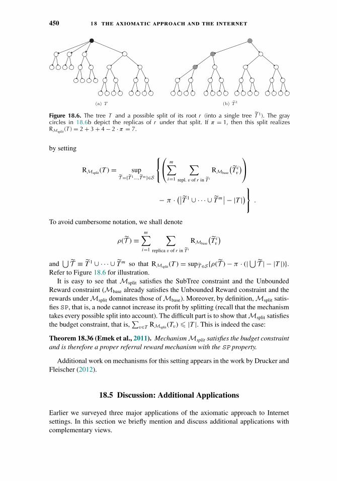
450 1 8 the axiomatic approach and the internet
(a) T (b) T 1
Figure 18.6. The tree T and a possible split of its root r (into a single tree T 1). The graycircles in 18.6b depict the replicas of r under that split. If π = 1, then this split realizesRMsplit (T ) = 2 + 3 + 4 − 2 · π = 7.
by setting
RMsplit (T ) = supT ={T 1...,T m}∈S
⎧⎨⎩⎛⎝ m∑
i=1
∑repl. v of r in T i
RMbase
(T i
v
)⎞⎠− π · (∣∣T 1 ∪ · · · ∪ T m
∣∣− |T |)⎫⎬⎭ .
To avoid cumbersome notation, we shall denote
ρ(T ) ≡m∑
i=1
∑replica v of r in T i
RMbase
(T i
v
)and
⋃T ≡ T 1 ∪ · · · ∪ T m so that RMsplit (T ) = supT ∈S{ρ(T ) − π · (|⋃ T | − |T |)}.
Refer to Figure 18.6 for illustration.It is easy to see that Msplit satisfies the SubTree constraint and the Unbounded
Reward constraint (Mbase already satisfies the Unbounded Reward constraint and therewards under Msplit dominates those of Mbase). Moreover, by definition, Msplit satis-fies SP, that is, a node cannot increase its profit by splitting (recall that the mechanismtakes every possible split into account). The difficult part is to show that Msplit satisfiesthe budget constraint, that is,
∑v∈T RMsplit (Tv) � |T |. This is indeed the case:
Theorem 18.36 (Emek et al., 2011). Mechanism Msplit satisfies the budget constraintand is therefore a proper referral reward mechanism with the SP property.
Additional work on mechanisms for this setting appears in the work by Drucker andFleischer (2012).
18.5 Discussion: Additional Applications
Earlier we surveyed three major applications of the axiomatic approach to Internetsettings. In this section we briefly mention and discuss additional applications withcomplementary views.

1 8 .5 discussion: additional applications 451
18.5.1 Normative Approach to Ranking Systems
Reasoning about agent preferences on a set of alternatives, and the aggregation ofsuch preferences into some social ranking is a fundamental issue in reasoning aboutmultiagent systems. When the set of agents and the set of alternatives coincide, weget the ranking systems setting for which we have explored the descriptive approachvia PageRank. Altman and Tennenholtz (2008) present an extensive axiomatic studyof the normative approach to such systems. In particular, two fundamental axiomsare considered: Transitivity and Consistency. Surprisingly, it is shown that there is nogeneral social ranking rule that satisfies both requirements. Furthermore, it is shownthat this impossibility result holds under various restrictions on the class of rankingproblems considered. However, when transitivity is weakened, an interesting positiveresult is obtained.
Incentive Compatibility
Altman and Tennenholtz (2007) introduce a study of incentives in ranking systems,where agents act in order to maximize their position in the ranking. Several basicproperties of ranking systems are considered, and fully characterize the conditionsunder which incentive compatible ranking systems exist, demonstrating that, in general,no system satisfies all the properties together.
Altman and Tennenholtz (2006) consider three measures for quantifying the incen-tive compatibility of ranking systems. These measures are applied to several knownranking systems, yielding tight bounds on their level of incentive compatibility. Thepaper also introduce two novel nonimposing ranking systems (i.e., in which eachagents’ ranking can be materialized), in which the measure of manipulation is suchthat manipulation is not severely harmful.
18.5.2 Selection Systems
In the selection system setting, agents elect representatives from within their groups.Voting profiles are represented by directed graphs over the set of agents, where anedge (i, j ) is taken to mean that agent i trusts or supports agent j . Given such a graph,the goal is to select a subset of agents of fixed size that maximizes the sum of inde-grees, that is, a subset of most popular or most trusted agents. On the other hand, eachagent is only interested in being selected, and may misreport its outgoing edges tothis end. This problem formulation captures realistic scenarios where agents chooseamong themselves, in the context of, for example, social networks such as Twitter,reputation systems such as Epinions, and Internet search (Alon et al., 2011; Fischerand Klimm, 2014) consider the design of mechanisms that satisfy two constraints: strat-egyproofness, that is, agents cannot benefit from misreporting their outgoing edges;and approximation, that is, the mechanism must always select a subset of agents that isclose to optimal in terms of the sum of indegrees. The paper shows a surprising impos-sibility: no deterministic strategyproof mechanism can yield a finite approximationratio for any k ∈ {1, 2, . . . , n − 1}, where k is the size of the selected subset and n isthe number of agents. However, the paper also shows that a randomized strategyproof

452 1 8 the axiomatic approach and the internet
mechanism yields an approximation ratio of four for any value of k, and provides aratio that approaches one as k grows.
18.5.3 Link Prediction
The link prediction problem is central to the field of complex network analysis. Linkprediction functions essentially map a graph to a ranking over pairs of vertices it. Highlyranked pairs constitute links that are likely to form, or may exist in the social network(such as Facebook friends the users have not yet reported about). Cohen and Zohar(2015) discuss the axiomatic approach to link prediction, and characterize several wellknown link prediction functions.
18.5.4 Trust Systems
Trust systems are in fact personalized ranking systems in which trust relations betweenmany agents are aggregated to produce a personalized trust rating of the agents. Altmanand Tennenholtz (2010) present an extensive axiomatic study of this setting, andexplores a wide array of well-known and new trust / personalized ranking systems.Several axioms are adapted from the literature on (global) ranking systems to thecontext of trust systems / personalized ranking systems, and fully classify the set ofsystems that satisfy all of these axioms. It is also shown that all these axioms arenecessary for this result.
18.5.5 Axioms for Collaborative Filtering
Pennock et al. (2000a) present several requirements from collaborative filtering meth-ods, and show that they fit the classical setting of social choice. This allows the authorsto deduce that the set of systems satisfying the related requirements is extremely nar-row. While this treatment is still in the setting of Arrow’s Theorem (applied before toother CS settings, see, e.g., Kfir-Dahav and Tennenholtz, 1996) it also illustrates thepower of axiomatization in Internet settings.

CHAPTER 19
Knockout Tournaments
Virginia Vassilevska Williams
19.1 Introduction
The theory of social choice has developed an immense variety of voting rules, rangingfrom simple rules such as plurality to more complicated rules such as the tournamentequilibrium set studied in Chapter 3. Even though the variety may seem vast, mostvoting rules can be grouped into a small number of types. The main two types are scoringrules and Condorcet-consistent rules (also called Condorcet extensions). The formercontain rules such as Borda and approval voting. A large portion of the latter type ofrules consists of majority rules that determine the winner by using pairwise comparisonsbetween candidates using the majority rule. Examples of such rules include the binarycup and the tournament solutions such as the Slater, Banks and uncovered sets (seeChapter 3).
Majority voting rules can be viewed as tournaments:1 competitions between thecandidates that determine the winner using some rule based solely on the results ofmatches, that is pairwise comparisons.
Besides as voting rules, tournaments are prevalent in many social settings, mostcommonly in sports competitions, but also in patent races (Lita, 2008; Durant, 2010),hiring employees (Ryvkin, 2010), and even drug trials (these are commonly referredto as “head-to-head” drug trials).
Tournaments have a wide variety of formats; their common feature is that theyproceed in stages. In each stage several pairwise comparisons called matches takeplace. As mentioned earlier, in social choice, a match is typically implemented by asimple majority rule. The outcome of the matches in a stage influences (using some rule)which matches take place in the next stage. In the final stage a winner is determined.Different types of tournaments differ in how matches in different stages are selectedand how the final winner is determined.
1 Unlike in Chapter 3, in this chapter, a tournament refers to a competition, and not to the majority graph whichwe call the tournament graph in this chapter.
453

454 1 9 knockout tournaments
A very common type of tournament is the so-called knockout or single-eliminationtournament. In a knockout tournament, no ties are allowed, so that every match producesa match winner. The important property of a knockout tournament is that once a playerloses a match, he is eliminated, that is, “knocked-out,” from the tournament. Thus thewinner of a knockout tournament has won all of her matches. Knockout tournamentsare typically represented by a binary tree the leaves of which are labeled by playersand each internal node is labeled by the winner between the two children. In socialchoice such a tree is called a voting tree or an agenda. (We give a formal definition ofa knockout tournament later.)
In this chapter we will focus on knockout tournaments and issues related to manip-ulating the winner that they pick by changing something about their structure. Thelatter is perhaps the most central topic in the study of knockout tournaments withincomputational social choice. Other topics around knockout tournaments are mentionedin Section 1.5.
19.2 Formal Definition and Some Properties
We begin by formally defining a knockout tournament.
Definition 19.1. Given a set C of m players, a knockout tournament (T , S) is definedby a binary tree T with m leaves L(T ) and a bijective function S : C → L(T ) calledthe seeding, mapping the m players to the m leaves. Suppose that in addition to C, foreach two u, v ∈ C one and exactly one of u and v is picked to be the winner of thematch between u and v. Then the winner of a knockout tournament (T , S) is determinedrecursively: the winner at a leaf l is the player j with l = S(j ), and the winner of thesubtree rooted at a node v is the winner of the match between the winners of the twosubtournaments rooted at the children of v.
In sports tournaments such as the tennis tournament Wimbledon or the basketballtournament March Madness, the tree T is often referred to as the bracket. There T istypically a complete balanced binary tree, and the seeding depends on the prior matchhistory of the players. In the sequential majority comparisons voting rule, T is a pathon n nodes with an extra edge attached to each node except the last, that is, in eachstage, a new candidate is compared to the current winner and if the current winnerloses, the new candidate replaces him.
Properties
As mentioned in the introduction, all natural majority voting rules are Condorcetextensions (see Chapter 2), that is, if there is a Condorcet winner, it is elected. This iseasy to see for knockout tournaments—regardless of the tree structure and the seeding,if a candidate is preferred over any other candidate by a majority of the voters, thenthat candidate will win all matches and will be the winner.
Knockout tournaments satisfy an even stronger property—they are Smith-consistent:if the set A of candidates is split into A1 and A2 = A \ A1 so that every candidate inA1 is preferred (by a majority) over every candidate in A2, then regardless of the

1 9 .2 formal definition and some properties 455
a b c d
a c
a
a d c b
d cc
a c b d
a dd
a always beats b and c.c always beats b and d, andd always beats a and b.
Figure 19.1. Here, for each of the three players that can beat at least two others, there is aseeding that guarantees that they can win. For seeding a, b, c, d, player a wins. For seedinga, d, c, b, player c wins, and for seeding a, c, b, d, player d wins.
seeding of the candidates at the leaves, a knockout tournament using pairwise majoritycomparisons always elects a candidate in A1. (The smallest nonempty set satisfyingthe requirement for A1 is called the Smith set or the top cycle; see Chapter 3.)
Knockout tournaments suffer from all the drawbacks of all resolute Condorcet-consistent voting rules—they do not satisfy the reinforcement and participation criteria(see Chapter 2 and Moulin, 1988a, pp. 237 and 239). Participation states that no voterhas an incentive to not vote. Reinforcement2 states that if the voter set N is split intotwo sets N1 and N2 that both elect a candidate a, then N should also elect a.
In addition, knockout tournaments have other drawbacks. For instance, asFigure 19.1 demonstrates, the seeding easily affects the winner, and because the seed-ing depends on the names of the candidates, knockout tournaments do not satisfyneutrality—renaming candidates can change the elected winner. They also do not sat-isfy Pareto-optimality when the number of candidates is at least 5, regardless of T andS (see Moulin, 1988a, p. 245, for a proof). That is, for any (T , S) on more than 5 candi-dates, there is a voter profile so that there is some other candidate that is unanimouslypreferred to the elected winner.
Regardless of all these problems, knockout tournaments are extremely popular,largely because of their simplicity. They are popular in sports also because of theirefficiency—the number of matches they require is no more than the number of players.They also have the advantage that no player has an incentive to intentionally lose amatch because a single loss causes elimination. (Other tournament formats such asdouble-elimination no longer have this property.) This also makes knockout sportstournaments exciting to watch as in most cases players try to play their best.
Computing the Probability of Winning
The definition of the winner of a knockout tournament is constructive and providesa linear time algorithm to find the winner for a given seeding, provided for any pair
2 Knockout tournaments not satisfying reinforcement means the following: there exists a set of candidates C, aset of voters N with preferences over C, a splitting of N into N1 and N2 = N \ N1 and a knockout tournament(T , S), such that if one uses either the preferences solely of N1 or solely of N2 to compute the winner of (T , S),then that winner is some candidate a, whereas if one uses the preferences of all of N , then the winner is adifferent candidate b.

456 1 9 knockout tournaments
of players a, b we can determine the winner of the match between a and b. Suppose,however, that we are given an m × m probability matrix P such that P [i, j ] is theprobability that i beats j , so that 0 � P [i, j ] = 1 − P [j, i] � 1. Can we determinewhich player has the maximum probability of winning the tournament?
The answer to this question turns out to be yes. In fact, there is an O(m2) timealgorithm that can calculate for any given seeding and player j , the probability that j
wins a tournament on m players defined by P . Given (T , S), P and a player j , oneruns the following dynamic programming algorithm.
Let q(j, v) be the probability that j reaches tree node v of T . For all players j , wehave that q(j, S(j )) = 1. If v is a node with children r and l, such that j is seeded ata descendent of r , then q(j, v) = q(j, r) ·∑i q(i, l) · P [j, i]. The runtime is O(m2)because i and j are only matched at the least common ancestor of their leaves.
Notice that the preceding algorithm does not depend on the structure of T , just onthe fact that T is binary. The structure of the tree T does play a role in some settings.For instance, if T is a balanced binary tree on � 4 candidates, then one can showthat it selects a Pareto-optimal candidate. In the next section we will show that if onecan manipulate the shape of T , then one can almost arbitrarily pick the winner of thetournament.
19.3 Agenda Control for General Knockout Tournaments
We mentioned earlier that no single player has an incentive to lose on purpose in aknockout tournament. However, one can imagine many other different types of manip-ulation of the tournament outcome. One type of manipulation defined by Bartholdiet al. (1989a, 1992) is called agenda control. Here, one considers how much power anelection chairman has in affecting the outcome of the election by changing somethingin the protocol itself.3 For the special case of knockout tournaments, the chairman (orthe tournament organizer) has the freedom to pick two things, the tree T and the seed-ing S. If the chairman can change T , then we can assume that the seeding is fixed byfixing an ordering of the leaves of T . Hence we will consider only two types of agendacontrol—when the chairman can change T , and when T is fixed but the chairman canchange S.
In order for the chairman to be able to control the agenda, we need to consider whattype of information he has about the pairwise comparisons.
In the deterministic setting most commonly used in social choice, we may assumethat the chairman has access to a tournament graph: a directed graph such that for anytwo vertices4 i and j exactly one of (i, j ) and (j, i) is an edge. The vertices of thetournament graph correspond to the players/candidates in the knockout tournament,and the tournament graph gives the match outcome for any pair of players. In the socialchoice setting, the tournament graph obtained by adding a directed edge from i to j ifand only if i is preferred to j by a majority of voters, is called the majority graph.
3 Agenda control should not be confused with the implementation by agenda problem discussed in Chapter 3.4 In this chapter we refer to vertices and nodes interchangeably.
1 9 .3 agenda control for general knockout tournaments 457
In a more general probabilistic setting, one is given a probability matrix P withrows and columns indexed by the candidates, so that P [i, j ] is the probability that i ispreferred to j . Here P [i, j ] � 0 and P [i, j ] + P [j, i] = 1 for all i, j .
Now, the general agenda control problem is as follows:
Definition 19.2 (General Agenda Control for Knockout Tournaments). Let thefollowing be given: a candidate i, a threshold p ∈ (0, 1], and voter profile information.The voter profile information can be a probability matrix P on the candidates, in whichcase we say it is probabilistic, or it can be a tournament graph G, in which case we sayit is deterministic and we can assume that p = 1. The general agenda control problemfor knockout tournaments asks to determine whether there is a knockout tournament(T , S) so that i wins (T , S) with probability at least p.
We refer to the problem as
� agenda control if the chairman can only modify S (T is fixed) and his input is determin-istic
� P -agenda control if the chairman can only modify S (T is fixed) and his input isprobabilistic
� full agenda control if the chairman can modify T and his input is deterministic� full P -agenda control if the chairman can modify T and his input is probabilistic
Each of these problems is in NP: when m is the number of candidates, it can besolved by guessing the tree T on m leaves and the seeding S of T , and then computingthe probability that the given candidate i wins for the given T and S. In the remainderof the chapter we will discuss the time complexity of the problems, that is, we will tryto address the question:
Is there an efficient algorithm that decides each of the preceding four variants of theagenda control problem?
Full Agenda Control
In this deterministic setting, there is a simple algorithm for full agenda control runningin time linear in the size of the tournament graph G. The algorithm does depth-first-search in G starting from the input candidate i and returns “yes” if and only if all nodesin G are reachable from i.
To see why this algorithm works, we will prove two claims. Claim 19.1 shows thatany winner of a knockout tournament is in the top cycle of the tournament graph.Claim 19.2 shows that any candidate in the top cycle is a winner of some knockouttournament. Claim 19.1 is proven for instance by Moulin (1988a), and Claim 19.2appears in Lang et al. (2007).
Claim 19.1. Suppose that (T , S) is a knockout tournament that i wins. Then in thetournament graph G, every node j is reachable from i.
Proof. We prove this by induction on the number of leaves of the tree. Base case: ifthe tree has a single leaf node, the candidate seeded at that leaf is the single node in thetournament graph so the claim is trivially true.
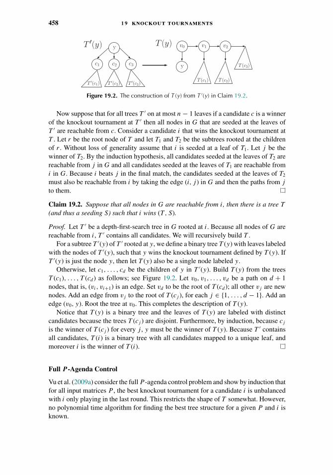
458 1 9 knockout tournaments
y
c1 c2 c3
T ′(c1) T ′(c2) T ′(c3)
v0 v1 v2
T (c3)
T (c1) T (c2)
y
T ′(y) T (y)
Figure 19.2. The construction of T (y) from T ′(y) in Claim 19.2.
Now suppose that for all trees T ′ on at most n − 1 leaves if a candidate c is a winnerof the knockout tournament at T ′ then all nodes in G that are seeded at the leaves ofT ′ are reachable from c. Consider a candidate i that wins the knockout tournament atT . Let r be the root node of T and let T1 and T2 be the subtrees rooted at the childrenof r . Without loss of generality assume that i is seeded at a leaf of T1. Let j be thewinner of T2. By the induction hypothesis, all candidates seeded at the leaves of T2 arereachable from j in G and all candidates seeded at the leaves of T1 are reachable fromi in G. Because i beats j in the final match, the candidates seeded at the leaves of T2
must also be reachable from i by taking the edge (i, j ) in G and then the paths from j
to them.
Claim 19.2. Suppose that all nodes in G are reachable from i, then there is a tree T
(and thus a seeding S) such that i wins (T , S).
Proof. Let T ′ be a depth-first-search tree in G rooted at i. Because all nodes of G arereachable from i, T ′ contains all candidates. We will recursively build T .
For a subtree T ′(y) of T ′ rooted at y, we define a binary tree T (y) with leaves labeledwith the nodes of T ′(y), such that y wins the knockout tournament defined by T (y). IfT ′(y) is just the node y, then let T (y) also be a single node labeled y.
Otherwise, let c1, . . . , cd be the children of y in T ′(y). Build T (y) from the treesT (c1), . . . , T (cd ) as follows; see Figure 19.2. Let v0, v1, . . . , vd be a path on d + 1nodes, that is, (vi, vi+1) is an edge. Set vd to be the root of T (cd ); all other vj are newnodes. Add an edge from vj to the root of T (cj ), for each j ∈ {1, . . . , d − 1}. Add anedge (v0, y). Root the tree at v0. This completes the description of T (y).
Notice that T (y) is a binary tree and the leaves of T (y) are labeled with distinctcandidates because the trees T (cj ) are disjoint. Furthermore, by induction, because cj
is the winner of T (cj ) for every j , y must be the winner of T (y). Because T ′ containsall candidates, T (i) is a binary tree with all candidates mapped to a unique leaf, andmoreover i is the winner of T (i).
Full P-Agenda Control
Vu et al. (2009a) consider the full P -agenda control problem and show by induction thatfor all input matrices P , the best knockout tournament for a candidate i is unbalancedwith i only playing in the last round. This restricts the shape of T somewhat. However,no polynomial time algorithm for finding the best tree structure for a given P and i isknown.
1 9 .3 agenda control for general knockout tournaments 459
Open Problem 19.3. Is the full P -agenda control problem in polynomial time?
P-Agenda Control
The P -agenda control has been extensively studied, especially for the case of balancedbinary trees. The complete balanced binary tree is the most widely used tournamenttree in practice. It is defined when the number of candidates/players is a power of 2, butthe concept can also be extended to arbitrary numbers 2i − k of players by allowingk players a bye, that is, these players play their first match in the second round of thetournament.
There are several reasons for why most knockout tournaments in sports are balanced.First, they are considered more fair, because in order to win the tournament, any playermust win exactly the same number of matches. In fact, Lang et al. (2007) call thewinners of balanced knockout tournaments “fair possible winners.” Another reasonis that balanced tournaments offer the maximum possible parallelism, so that thetournament can be scheduled to last the shortest possible time.
The history of the P -agenda control problem for balanced binary trees is as follows.First, several papers proved that the P -agenda control problem is NP-complete (Langet al., 2007; Hazon et al., 2008) for arbitrary P . Vu et al. (2009a) then showed thatthe P -agenda control problem is NP-complete even when the probabilities in P are in{0, 1, 1/2}. Finally, in a breakthrough result, Aziz et al. (2014e) showed that even theagenda control problem for balanced binary trees (i.e., when P is just over {0, 1}) isNP-complete.
Besides putting a restriction on the values in P , one can also restrict P in a differentway. Suppose that we have some order of the players, so that we think of player i
as stronger than any player j > i, then a natural way to capture this is to enforce amonotonicity property on the probability matrix P . Intuitively, if i is at least as strongas j > i, then we would like that i beats j with probability at least 1/2. Moreover, forany other player k, we would expect that k has a harder time beating i than beating j ,that is, P [k, i] � P [k, j ]. This motivates the following definition.
Definition 19.3. A probability matrix P is monotonic if
� P [i, j ] � 1/2 for i < j� P [i, j ] � P [i, k] for every i and j < k
A matrix is monotonic exactly when it is sorted in each row and column and hasentries � 1/2 above the diagonal. A natural question is whether the P -agenda controlproblem is still NP-complete when we restrict ourselves to monotonic matrices P , aswe would expect probability matrices arising from practical applications to be roughlymonotonic. It turns out, however, that the complexity of this version of the problem isstill unknown.
Open Problem 19.4. Is the P -agenda control polynomial time solvable when P ismonotonic?

460 1 9 knockout tournaments
v1
u1
v2
u2
v3
u3
v4
Figure 19.3. An example of an SMC-tree with seven vertices.
Consider relaxing the monotonicity property by allowing for the rows and columnsto be “roughly” sorted up to some noise. (From a practical perspective, this makessense as in the real world there is always noise.) One way to define such a relaxationis that if j < k then for all i, P [i, j ] is at most P [i, k], plus some slack ε.
Definition 19.4. A probability matrix P is ε-monotonic if
� P [i, j ] � 1/2 for i � j� P [i, j ] � P [i, k] + ε for every i and all j < k
As ε goes closer to 0, such a matrix P becomes closer and closer to monotonic.Interestingly, Vu et al. (2009a) showed that P -agenda control for ε-monotonic P forany ε > 0 is NP-complete, thus almost settling Open Problem 19.4.
Even though the P -agenda control problem is NP-complete even for very structuredmatrices, it is still interesting to consider how fast it can be solved. Even if P �= NP,it could be that there is a subexponential, that is, O(2εm) time algorithm for all ε > 0,which although not polynomial, is still extremely fast.
Open Problem 19.5. Is the P -agenda control problem in subexponential time?
Agenda Control
In the previous paragraph we noted that the agenda control for balanced binary trees isNP-hard (Aziz et al., 2014e). In the following, we show that there exist natural trees T
for which the agenda control problem is efficiently solvable. Thus, the complexity ofthe agenda control problem crucially depends on the tree.
Recall the sequential majority comparisons rule from the previous section. Thebinary tree associated with its tournament is a directed path v1 . . . , vm on m nodes withan extra edge (vi, ui) attached to each vi for i < m. We will call this tree an SMC-tree.See Figure 19.3 for an example. The following claim shows that the chairman canalways efficiently manipulate the outcome of a sequential majority election.
Claim 19.6. If T is an SMC-tree, then the agenda control problem for any tournamentgraph G and candidate i can be solved in polynomial time.
Proof. Given G = (V, E) on m nodes, let us first compute the strongly connectedcomponents of G. This can be done in O(m2) time as G has O(m2) edges. The stronglyconnected components form a directed acyclic graph, the SCC-DAG. The nodes of theSCC-DAG are the strongly connected components, and there is a directed edge from
1 9 .3 agenda control for general knockout tournaments 461
C to C ′ if and only if there is some u ∈ C, v ∈ C ′ with (u, v) ∈ E. We will show thati is a winner of a knockout tournament if and only if i is in the unique source node ofthe SCC-DAG of G.
As we proved in Claim 19.1, if i is a winner of a knockout tournament, regardless ofthe structure of T , i must have a path in G to all other nodes. Thus i is in a source nodeof the SCC-DAG, and because G is a tournament graph this source node is unique.
On the other hand, suppose that i is in the unique source node of the SCC-DAG.We will show that one can construct (in polynomial time) a Hamiltonian path in G
starting from i. (This also proves that tournament graphs always contain a Hamiltonianpath and one can be found in polynomial time.) After this, from the Hamiltonian pathstarting from i we will construct a seeding of an SMC-tree on m leaves so that i
wins, as follows. If there is a Hamiltonian path in G starting from i, let this path bei = x1 → x2 → . . . → xm. For each j < m, seed xj at leaf uj of the SMC-tree, andseed xm at vm. It is easy to see by induction that xj wins the tournament rooted atthe parent of its leaf node, and hence i wins the knockout tournament defined by theseeded SMC-tree.
Now, let us show that if i is in the source node of the SCC-DAG, then one can find aHamiltonian path in G starting with i. Consider G′ = G \ {i}. G′ is still a tournamentgraph. By induction, assume that for any vertex j in the source node C of the SCC-DAGof G′ we can construct a Hamiltonian path of G′ starting from j . This is true for thebase case when G′ has only one vertex. Now, because i can reach all nodes in G, andall edges incident to C in G′ go out of C, i must have an out-neighbor j ∈ C. Build theHamiltonian path P in G′ starting from j . Then i, followed by the edge (i, j ) followedby P is a Hamiltonian path of G.
Although some variants of the agenda control problem are NP-hard, NP-hardnessonly implies that (unless P = NP) there is no polynomial time algorithm for theproblem. How fast can one solve the problem in general? Is exponential time necessaryfor some T ? It is not hard to devise a dynamic programming algorithm that solvesthe agenda control problem for arbitrary T in O(3mpoly(m)) time. We describe this inwhat follows.
Theorem 19.7. Given any tree T , the agenda control problem for T can be solved inO(3mpoly(m)) time.
Proof. One computes a table entry σ (u, U, j ) for every node u of T , subset U ofthe players and every j ∈ U . σ (u, U, j ) represents a seeding of the leaves of thesubtournament Tu of T rooted at u with the players of U for which j wins thetournament Tu. Here we can assume that |U | is exactly the number of leaves |L(Tu)|of Tu, and σ (u, U, j ) = ∅ if j cannot win Tu.
If |Tu| = 1, then set σ (u, {j}, j ) = {j} for all j . Otherwise, suppose that for someinteger s � 1 we have computed σ (v, S ′, i) for all v ∈ T , S ′ ⊆ V and i ∈ S ′ suchthat |S ′| = |L(Tv)| < s. We show how to compute σ (u, S, j ) for any particular u ∈ T ,S ⊆ V and j ∈ S with |S| = |L(Tu)| = s.
Let v and w be the children of u and let s ′ = |L(Tv)|, so that |L(Tw)| = s − s ′.Consider all subsets U ⊆ S such that |U | = s ′. Because s ′, s − s ′ < s, we have alreadycomputed σ (v, U, i) for all i ∈ U and σ (w, S \ U, k) for all k ∈ S \ U .

462 1 9 knockout tournaments
Now, for each choice of U with |U | = s ′, j ∈ U such that σ = σ (v, U, j ) �= ∅, wego through all i ∈ S \ U such that j beats i. If σ (w, S \ U, i) �= ∅, then set σ (u, S, j ) =σ 1 σ (w, S \ U, i). That is, if there is a seeding for U such that j wins Tv and a seedingof S \ U such that i wins Tw and j beats i, then the concatenation of those seedings isa seeding for which j wins Tu.
If no choice of U with j ∈ U works, do the same for choices for U with |U | = s ′,j /∈ U , reversing the roles of v and w. Finally, if no partitioning of S gives a goodseeding for j , then j cannot win the tournament on S with tree Tu, so set σ (u, S, j ) = ∅.
Let us analyze the running time. For each node u of T , we consider all subsets S
of size t = |L(Tu)| and to compute σ (u, S, j ) for some j ∈ S in the worst case weconsider all possible 2t subsets of S. (For some special cases of T we may considerfewer subsets.) The runtime per subset U of S is O(t). Thus the final runtime over allchoices of u, t , S of size t and j ∈ S is asymptotically
m∑t�m
t
(m
t
)2t · t � m3
∑t�m
(m
t
)2t1m−t � m33m.
The fastest known algorithm for the agenda control problem for complete balancedtrees is by Vassilevska Williams (2009) and runs in O(2mpoly(m)) time and uses sophis-ticated machinery such as fast subset convolution (Bjorklund et al., 2007). However,the algorithm of Vassilevska Williams (2009) uses �(2mpoly(m)) space. Aziz et al.(2014e) present a family of algorithms for the agenda control problem for completebalanced trees with a sophisticated time/space trade-off. The fastest of their algorithmsruns in O(2.8285m) time and uses O(1.7548m) space.
The algorithm in Theorem 19.7 and the algorithms of Vassilevska Williams (2009)and Aziz et al. (2014e) can be made to count the number of seedings for which the givenplayer wins. This counting version of the agenda control problem is called #AgendaControl.
Definition 19.5. The #Agenda Control problem is as follows: given a tournament graphG, a tree T and a node v ∈ G, count the number of seedings of T for which v wins thetournament defined by T , using the match outcomes given by G.
The number of winning seedings for a player is an extremely interesting measure. Forinstance, it immediately gives the probability that the player will win a randomly seededtournament given by T . Being able to compute the count efficiently would give aninteresting new way of ranking players. Unfortunately, even when we restrict ourselvesto complete balanced trees, computing the count exactly is NP-hard by the resultof Aziz et al. (2014e) mentioned earlier. What about approximations? Unfortunatelyagain, Aziz et al. (2014e) also show that, unless RP = NP, there is not even a fullypolynomial randomized approximation scheme (FPRAS) for the problem, that is, analgorithm that for all ε > 0, returns in poly(m, 1/ε) time a value that is betweenc/(1 + ε) and (1 + ε)c where c is the true answer. Thus #Agenda Control is a truly hardproblem.
In the rest of the chapter we will focus on the natural special case of the agendacontrol problem for complete balanced trees and will present two cases for which the

1 9 .4 agenda control 463
a
ab
cd
ef
gh
a b c d
a c
a
e f g h
e ge
Figure 19.4. A seeded balanced knockout tournament and its outcome, and its correspondingbinomial tree.
problem is actually efficiently solvable, thus circumventing the NP-hardness result ofAziz et al. (2014e).
Balanced Tournament Agenda Control as a Graph Problem
Recall that a player v can win the tournament under some seeding if and only if thereis a partition of the players V into S and V \ S with v ∈ S and |S| = m/2 such that
� v can win a balanced knockout tournament on S under some seeding� there is a player u ∈ V \ S that v beats and u can win a balanced knockout tournament
on V \ S under some seeding
Consider the tournament graph G of match outcomes. Because v beating u is thesame as the existence of the directed edge (v, u) in G, the preceding conditions areequivalent to the existence of a tree of a particular shape, rooted at v, with edges directedaway from v spanning the entire graph. This tree is a binomial spanning arborescenceof G rooted at v.
A binomial arborescence is the directed version of binomial trees as in Knuth (1973).A binomial arborescence on m nodes rooted at a node v is recursively built by takingtwo disjoint binomial arborescences on m/2 nodes, one rooted at v, and one rooted at anode u, and then adding the directed edge (v, u). The smaller binomial arborescencesrepresent the two subtournaments that u and v win, and the edge (v, u) represents thefinal match between them. See Figure 19.4 for an illustration.
Thus the balanced tournament agenda control problem is equivalent to the following.
Definition 19.6 (Tournament Fixing Problem (TFP)). Given a tournament graph G
and a node v, is there a binomial arborescence rooted at v, spanning G?
19.4 Agenda Control for Balanced Trees Is Easyfor Special Instances
This section provides some proofs that in some cases agenda control for balanced treesis easy. We will consider two different types of results. The first type are structural
464 1 9 knockout tournaments
results of the following form: suppose that the tournament graph G or the given playeri have some special property, then there always exists a seeding for which i can winthe balanced tournament, and this seeding can be found efficiently.
The second type of results are of the following distributional form: consider aspecial probabilistic model for generating majority graphs, then for almost all graphsgenerated by the model, one can always efficiently find a winning seeding for all (ormost) players.
19.4.1 Structural Results
Our goal in this section is to consider various notions of strength that a candidatehas so that regardless of the individual match outcomes, there is always an efficientlycomputable winning balanced knockout tournament seeding for any candidate thatfulfills the strength criterion.
A requirement for any winner w of a balanced knockout tournament is that in thetournament graph there is a path of length at most log m between w and all othercandidate/player nodes. A natural notion of strength that we can glean from this is thata node is strong if there are short paths between it and all other nodes. The strictestsuch strength notion is that the player should be a Condorcet winner—in this case thenode has distance 1 to all other nodes. The next strictest such strength notion is thatthe player should be a king.
Definition 19.7. A king is a node that has a path of length at most two to any othernode.
Every tournament graph contains a king as any node that beats the maximum numberof other nodes (i.e., every Copeland winner) is a king. To see this, let K be a Copelandwinner and let b be any node that beats K. Then b cannot beat every node that Kbeats, as otherwise it would have outdegree that is at least 1 larger than that of K,contradicting the fact that K is a node of maximum outdegree.
In fact, if there is no node that beats all other nodes, that is, if there is no Condorcetwinner, there are at least three kings in any tournament graph. The set of kings is alsocalled the uncovered set (see Chapter 3).
Although in general the tournament fixing problem is NP-hard, in the NP-hardnessproof of Aziz et al. (2014e) the desired winner of the tournament has long shortestpaths to some nodes in the tournament graph instance, so that it is far from being aking. Nevertheless, we can show that the tournament fixing problem is also NP-hardwhen the favorite player is a king. The proof of the theorem is due to Kim (2014).
Theorem 19.8. The agenda control problem for balanced binary trees is NP-hard evenwhen the given player is a king in the tournament graph.
Proof. We will reduce from the agenda control problem where the desired winner isnot necessarily a king. Let G be the given tournament graph on m nodes, and let v
be the desired winner. Let H be a transitive tournament on m new nodes and let u bethe unique node of outdegree m − 1 in H . Add a directed edge from v to u, and forevery x ∈ H and y ∈ G add a directed edge (x, y) (except for (u, v) which we alreadyfixed in the opposite direction). Let this new tournament graph be G′. First note that

1 9 .4 agenda control 465
v is now a king in G′, as it beats u and u beats everyone but v. Second, if there is aseeding of G for which v is a winner of a balanced single-elimination tournament overG, then this seeding can be completed to a winning seeding for v over G′ by arbitrarilyseeding the players of H in the second half of the bracket. Then v wins the first half ofthe tournament, u wins the second and then v beats u in the final.
Suppose on the other hand that there is a seeding for which v can win a balancedtournament over G′. Then in this seeding, every player of H must be in the same halfof the bracket, and the players of G must be in the other half. To see this, suppose thatwithout loss of generality u is in the left half of the seeding, and some nodes of H arein the right half of the seeding. Then, because every node of H \ {u} beats every nodeof G, the winner of the right half of the tournament bracket is some node h ∈ H \ {u}.However, this is already a contradiction, because this means that h will play in thefinal, and even if v is in the final, it would lose to h. Thus, one half of the seedingis a seeding solely of G which v must win, thus v can win G′ if and only if v canwin G.
In this section we consider some further restrictions on the king node that make theplayer strong enough to always be a winner of a balanced knockout tournament.
In the following, we assume that the number m of vertices of G is a power of 2. Wealso let the input player to the agenda control problem be a king K, and introduce thenotation A = Nout (K) and B = Nin(K) for the out- and in-neighborhood of K.
In all of the results in this section we use the following representation of a seedingof a knockout tournament. When one has deterministic match outcome information,the seeding permutation is equivalent to specifying which matches occur in eachof the log m rounds of the tournament. The matches in round i are m/2i disjoint edgesin the match outcome tournament graph, that is, a matching of size m/2i . Because eachmatching consists of directed edges, we let for each matching M , sources(M) denote{u | ∃v with (u, v) ∈ M}. If M is the set of matches played in round r , then the playerssurviving till round r + 1 is exactly sources(M). Let V (M) denote the vertices thathave incident edges in M . We thus use the following representation of a seeding.
Definition 19.8 (Matching Representation of a Seeding). A seeding in a balancedknockout tournament on m players with match outcomes from a tournament graph T
is represented by a set of tuples S = {(M1, 1), . . . , (Mlog m, log m)} where
� for each r , Mr is a matching of size m/2r in T� V (Mi+1) = sources(Mi)
Here if (M, r) ∈ S, then M are the set of matches to be played in round r . Adding theround number is redundant—we could have just had S be an ordered set of matchings.We add the round so that the algorithms would be easier to read.
In the following, we sometimes abuse notation and use M to denote V (M) when itis clear from the context that we are talking about vertices.
For a node v and subset S of the vertex set, we denote by NinS (v) the set of in-
neighbors of v that are in S. Similarly, NoutS (v) denotes the set of out-neighbors of v
that are in S. We denote |NinS (v)| by indegS(v) and |Nout
S (v)| by outdegS(v).

466 1 9 knockout tournaments
Algorithm SuperSeed(G,K):
1. If E(G) = {(K, a)} for some a, then
return ({(K, a)}, logm).
2. A = NoutG (K)
3. B = N inG (K)
4. Pick some a ∈ A , and set M = {(K, a)}.5. M = maximal matching from A \ {a} to B
6. MA = maximal matching within A \ {a} \M7. MB = maximal matching within B \M8. M = M ∪M ∪MA ∪MB
9. If |B \M | is odd, then let x ∈ B \M ,
y ∈ A \M and set M = M ∪ {(x, y)}.10. Return {(M, logm− log |G| + 1)} ∪
SuperSeed(G[sources(M)],K).
K
MA
MB
M
a
x
yA
B
Figure 19.5. Algorithm SuperSeed picks a winning seeding for any given superking K in G.
Superkings
The notion of a king K required that each node has at least one path of length at most2 from K. Here we define a stronger notion that requires that all nodes that are notout-neighbors of K have at least log m paths of length 2 from K.
Definition 19.9. A node K in an m-node directed graph is a superking if for everyb /∈ Nout (K), there are at least log m nodes c ∈ Nout (K) such that (c, b) is an edge.
Superkings do not necessarily exist in tournament graphs. However, if a node isa superking, then finding a winning seeding for it is relatively simple. We give thealgorithm for constructing a winning seeding in Figure 19.5, and it serves as a warm-up for the later more complicated construction.
Let m and K be global variables denoting the number of players in the originaltournament and K is the given superking player. The algorithm is as follows.
Theorem 19.9 (Vassilevska Williams, 2010). Algorithm SuperSeed computes in poly-nomial time a winning knockout tournament seeding for any superking K.
Proof. The runtime is polynomial because in each recursive call the size of the graphreduces in half, and because each individual step takes polynomial (in fact linear) time.It remains to show that the computed seeding makes the superking K the winner. Weprove this by induction. The base case is when G is a single edge. Then the only seedingis to match the two players against each other, as step 1 does.
Suppose now that for all tournament graphs on k vertices the algorithm produces awinning seeding for a superking. Then, we will show that given a graph on 2k vertices,SuperSeed picks a perfect directed matching M containing K as a source and K is stilla superking in the graph induced by the sources of M . Because the latter graph has k
vertices, it follows that SuperSeed returns a winning seeding for K in it, and combinedwith M this gives a winning seeding for K in the entire graph.
First, we show that the matching M produced by SuperSeed is a perfect matching.All we need to do is to show that step 9 completes M to a perfect matching. If |B ′ \ M ′|
1 9 .4 agenda control 467
is odd, because M has an even number of vertices and because G has an even numberof vertices, |A′ \ M| must also be odd. After step 8, however, all but at most one nodeof B ′ and at most one node of A′ are matched. Hence |A′ \ M| = |B ′ \ M| = 1, andstep 9 just maps the two vertices from these two sets. The direction of the edge (x, y)is also correct because M ′ was a maximal matching.
Now we show that if K is a superking in G, then it is also one in G[sources(M)].Consider any b ∈ B ′. As K is a superking, A′ \ {a} must contain at least log |G| − 1in-neighbors of b. If b ∈ sources(M), then b was not matched by M ′, and becauseM ′ is a maximal matching, all of the in-neighbors of b that are in A′ \ {a} are alsoin sources(M). Thus b has at least log |G| − 1 = log(|G|/2) in-neighbors in A′ ∩sources(M). As |sources(M)| = |G|/2 because M is a perfect matching, this makes Ka superking in G[sources(M)].
As we will see later on, even though superkings may seem like a restrictive notion,most nodes are superkings in almost all tournament graphs generated by a naturalrandom graph model.
Kings of Highish Outdegree
Here we give a second clean condition under which a king player can be made a winner.Let Hin(a) be the set of in-neighbors of a that have higher outdegree than a. We showthat if K is a node in a tournament graph such that outdeg(K) � |Hin(K)| + 1, thenthere is an efficiently constructible seeding for which K can win a balanced knockouttournament. We present a simplified version of the original proof of Stanton andVassilevska Williams (2011).
Theorem 19.10 (Kings of Highish Outdegree). Let G be a tournament graph and Kbe a king. If outdeg(K) � |Hin(K)| + 1, then one can efficiently compute a winningknockout tournament seeding for K.
This result is tight in the sense that there are tournament graphs and kings K withoutdeg(K) = |Hin(K)| such that K loses the tournament regardless of the seeding. Anexample of this is Figure 19.6. In this figure, K beats exactly m/2 − 1 nodes and losesto m/2. There is a player a that K beats that beats all players in Nin(K), and all playersin Nout (K) \ {a} lose to everyone in Nin(K). Each player in Nin(K) beats at least oneother player in Nin(K), so that the outdegree of each player in Nin(K) is at least m/2.Thus, Hin(K) = Nin(K) and outdeg(K) = |Hin(K)|. If K is to be the winner, everyplayer in Nin(K) must be eliminated either by a player in Nin(K) or by a. However,this means that a must survive at least log(|Nin(K)| + 1) > (log m) − 1 rounds, andhence will be the winner of the tournament because the tournament has exactly log m
rounds. Thus K cannot win, regardless of the seeding.An interesting special case of Theorem 19.10 is when K is a king that beats at least
half the graph, that is, m/2 players. Figure 19.6 also shows that there are graphs inwhich even if a king beats m/2 − 1 other players, he cannot win regardless of theseeding, so in that special case the result is tight as well.
We give a new algorithm, Algorithm Seed (Figure 19.7) and the algorithm ofTheorem 19.10 just runs Seed on input (G,Hin(K),K).
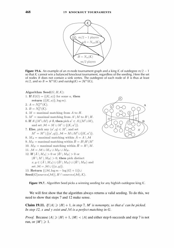
468 1 9 knockout tournaments
K
m/2 players
m/2 − 1 playersaA = Nout(K)
B = Nin(K)
Figure 19.6. An example of an m-node tournament graph and a king K of outdegree m/2 − 1so that K cannot win a balanced knockout tournament, regardless of the seeding. Here the setof nodes B does not contain a sink vertex. The outdegree of each node of B is thus at leastm/2, and so B = Hi n(K) and outdeg(K) = |Hi n(K)|.
Algorithm Seed(G,H,K):
1. If E(G) = {(K, a)} for some a, then
return ({(K, a)}, logm).
2. A = NoutG (K).
3. B = N inG (K).
4. M = maximal matching from A to H.
5. M = maximal matching from A \M to B \H.
6. If A\(M ∪M) = ∅, then pick a ∈ A\(M ∪M),
and set M = M ∪M ∪ {(K, a )}.7. Else, pick any (a , q) ∈ M , and set
M = M \{(a , q)}, M = M∪M ∪{(K, a )}.8. MA = maximal matching within A = A \M9. MB = maximal matching within B = B\H\M10. MH = maximal matching within H = H \M .
11. M = M∪MA ∪MB ∪MH .
12. If |A \MA| > 0 or |B \MB | > 0 or
|H \M \MH | > 0, then pick distinct
x, y ∈ (A \MA) ∪ (B \MB) ∪ (H \MH) and
set M = M∪ {(x, y)}.13. Return {(M, logm− log |G| + 1)}∪Seed(G[sources(M)], H ∩ sources(M),K).
K
MA
MB
M
a
x
y
A
B
H
M
MH
Figure 19.7. Algorithm Seed picks a winning seeding for any highish outdegree king K.
We will first show that the algorithm always returns a valid seeding. To do this, weneed to show that steps 7 and 12 make sense.
Claim 19.11. If |A| � |H | + 1, in step 7, M ′ is nonempty, so that a′ can be picked.In step 12, x and y exist and M is a perfect matching in G.
Proof. Because |A| � |H | + 1, |M| < |A| and either step 6 succeeds and step 7 is notrun, or |M ′| � 1.
1 9 .4 agenda control 469
For step 12, consider the parity of |A| + |B| + |H |. Here m is even, and m =|A| + 1 + |B| = (|A \ M \ M ′ \ {a′}| + |M| + |M ′| + 1) + 1
+ (|B \ H \ M ′| + |M ′| + |H \ M| + |M|)= |A| + |B| + |H | + 2(|M| + |M ′| + 1),
and hence |A| + |B| + |H | must be even.Thus either 0 or 2 of |A|, |B|, |H | are odd. Hence in step 12, if |A \ MA| > 0 (i.e.,
|A| is odd) or |B \ MB | > 0 (i.e., |B| is odd) or |H \ M \ MH | > 0 (i.e., |H | is odd),then exactly two of these are the case. Thus in step 12, x and y exist and moreover(A \ MA) ∪ (B \ MB) ∪ (H \ M \ MH ) = {x, y}, and adding (x, y) to M makes M aperfect matching.
This claim implies that the algorithm gives a valid seeding. To show that the seedingis in fact a winning seeding for K, we will show that an invariant is preserved by thealgorithm.
Lemma 19.12. Algorithm Seed preserves the following invariant:
|A| � |H | + 1, K is a king and the subset of nodes from NinG (K) that have larger
outdegree than K is contained in H .
If the invariant is maintained, K remains in G after each iteration, so that when|G| = 1, G contains only K, and the algorithm computes a winning seeding.
Before we begin the proof of Lemma 19.12, let us assert the following fact.
Claim 19.13. For any b ∈ B,
outdeg(b) � outdeg(K) ⇐⇒ outdegB(b) < indegA(b).
The proof of the claim is simple: outdeg(b) = 1 + outdegA(b) + outdegB(b) = 1 +outdeg(K) − indegA(b) + outdegB(b).
Proof of Lemma 19.12. Let us assume that in some iteration of the algorithm we havethat |A| � |H | + 1, K is a king and the subset of nodes from Nin
G (K) that have largeroutdegree than K is contained in H .
We will first show that |A ∩ sources(M)| > |H ∩ sources(M)| which of courseimplies |A ∩ sources(M)| � |H ∩ sources(M)| + 1.
|A ∩ sources(M)| � !(|A| + |M| + |M ′| − 1)/2" � (|A| + |M| + |M ′| − 2)/2
because all of A ∩ (M ∪ M ′) survive and the !(|A| − 1 − |M| − |M ′|)/2" sources ofMA survive. On the other hand,
|H ∩ sources(M)| � %(|H | − |M|)/2& � (|H | − |M| + 1)/2
because the only nodes of H that survive are the sources of MH and potentially a singleextra node if |H | − |M| is odd.
If |A| � |H | + 2, then because |M| � 1, (|A| + |M| + |M ′| − 2)/2 � (|H | +|M|)/2 = (|H | − |M| + 2|M|)/2 > (|H | − |M| + 1)/2, so that |A ∩ sources(M)| >
|H ∩ sources(M)|.
470 1 9 knockout tournaments
Otherwise, assume that |A| = |H | + 1. Then, if |M| + |M ′| � 2,
|A ∩ sources(M)| � |A|/2 = (|H | + 1)/2 > (|H | − |M| + 1)/2
� |H ∩ sources(M)|.
The final case is that |A| = |H | + 1, |M| = 1 and |M ′| = 0. In this case, |A ∩sources(M)| � !(|H | + 1)/2" and |H ∩ sources(M)| � %(|H | − 1)/2& � |H |/2.Because |A| and |B| have different parities, there are only two cases: either B = H , orthere are at least two nodes b and b′ in B \ H .
Suppose that B = H . Then, |B| < |G|/2 and |H ∩ sources(M)| � |H |/2 =|B|/2 < |G|/4, so that |A ∩ sources(M)| � |G|/2 − 1 − |H ∩ sources(M)| �|G|/4 > |H ∩ sources(M)|.
Suppose now that there are two nodes b and b′ in B \ H . Without loss of generality,assume that b beats b′. Thus outdegB(b) � 1. But then by Claim 19.13, we must havethat b has at least two in-neighbors from A, so that if |H | > 1, then there is a node tomatch K to, while matching b to an in-neighbor from A, and |M ′| � 1 but we assumedthat |M ′| = 0. Thus we must have that |H | = 1. But then, consider B \ H . Becausethe number of nodes in G is a power of 2, we must have that |B \ H | = |G| − 4 � 4.However, then there is a node b ∈ B \ H with outdegB(b) � 2. By Claim 19.13 thiswould imply that indegA(b) � 3 > |A|, a contradiction. Thus this case never occurs.
We have shown that the algorithm maintains that |A| � |H | + 1. Now let’s considersome node b ∈ Nin
G (K) that survives the iteration, in the sense that is among thesources of the matching M. We need to show that b must have at least one in-neighborin A ∩ sources(M), and that if b /∈ H , then its outdegree in the remaining graph is atmost that of K.
Consider the outdegree of b at the beginning of the iteration. Because b was notincluded in M ∪ M ′, all but possibly one of its in-neighbors (a′) are in sources(M).Thus, if b survived by beating another node of B, then its indegree from A must havebeen at least 2 by Claim 19.13 and thus b must have an in-neighbor in A ∩ sources(M).If on the other hand b survived by beating a node in A, then step 7 did not happenand no node a′ is removed from M ′. Thus all of the in-neighbors of b from A are insources(M). This proves that K is still a king after the iteration.
Now consider a node b ∈ B \ H that survives the iteration and is in sources(M).Because outdeg(b) � outdeg(K), by Claim 19.13, outdegB(b) < indegA(b). We willshow that after the iteration outdegB∩sources(M)(b) < indegA∩sources(M)(b), completingthe proof via Claim 19.13.
If all in-neighbors of b from A also survive the iteration, then
outdegB∩sources(M)(b) � outdegB(b) < indegA(b) = indegA∩sources(M)(b).
We can therefore assume that Step 7 of the algorithm occurs and that a′ was an in-neighbor of b that did not survive. Because all other in-neighbors of b survive, wehave that indegA∩sources(M)(b) = indegA(b) − 1. However, because Step 7 happenedand b still survived, it must have done so by beating an out-neighbor in B. ThusoutdegB∩sources(M)(b) � outdegB(b) − 1 < indegA(b) − 1 = indegA∩sources(M)(b). Thiscompletes the proof. �

1 9 .5 extensions and further reading 471
19.4.2 Distributional Results
So far we have only considered worst case inputs to the agenda control problem. It isnatural to ask how the complexity of the problem changes if instead the input is takenfrom a probability distribution.
For tournament problems, an extremely natural probabilistic generative model wasproposed by Condorcet as follows. The players are totally ordered from 1 to m. Letp be a value less than 1/2. Then, a tournament graph T is sampled as follows. Foreach i, j with i < j , a directed edge (i, j ) is added to T with probability 1 − p andotherwise, with probability p, edge (j, i) is added.
This model attempts to capture real-world scenarios, where there is a hidden totalorder of the players but we observe a noisy sample of it, so that with some smallprobability p, a weaker player actually beats a stronger one, but otherwise, strongerplayers beat weaker players.
Consider the agenda control problem for balanced knockout tournaments restrictedto inputs generated in this way. For any player w and any seeding, apriori the probabilitythat w wins the tournament is at most (1 − p)log m � 1/mγ for some γ (depending onp) even for the strongest player. Hence no fixed seeding can give a good probabilityof winning for w for all tournaments generated by the Condorcet model. The situationchanges, however, if we are allowed to see the tournament graph T generated by themodel. Then one can show that with high probability, T has some structure so that evenfor very small p, one can find a winning seeding for every player!
Theorem 19.14 (Every Node Is a Winner). Let p = C√
log m/(m − 1) for C � 8.Then for almost all tournament graphs T generated by the Condorcet model, for everyplayer w in T , there is an efficiently computable seeding for which w wins the balancedknockout tournament with outcomes given by T .
The proof of the preceding theorem appears in Vassilevska Williams (2010). Itis based on showing, using standard Chernoff bounds, that in a tournament graphgenerated with p = C
√log m/(m − 1) with C > 8, with high probability, every vertex
is a superking.The theorem requires that p � �(
√log m/m). Can anything be said for smaller
values of p? In order for the weakest player vm to be able to win, it needs to beable to win at least log m matches. In order for this to happen with good probability,p must be �(log m/m). Such low probability is not sufficient to make every playera possible winner. However, Stanton and Vassilevska Williams (2011) show that ifp � �(2i log m/m) for some positive integer i, then any one of the top 1 + m(1 − 1/2i)players have a winning seeding.
19.5 Extensions and Further Reading
There has been a lot of experimental work on tournament seeding. Russell (2010),for instance, extends the distributional results presented in the previous section. Hegenerates tournament graphs from real data and shows experimentally that the agendacontrol problem for the generated tournaments is typically easily solved, even when
472 1 9 knockout tournaments
one places restrictions on the tournament organizer. The restrictions can be of manydifferent types: some players may be required to play each other before facing anyoneelse; there may be strict rules on positioning the teams, for instance that geographicallyclose-by teams should play each other, and so on. Russell’s results indicate that theagenda control problem may be easy in real life, even if the tournament organizer’shands may seem tied. One catch here is, of course, just as with the distributionalresults from the previous section, that the tournament organizer needs to be able tosee the actual outcomes. Nevertheless, it could be that the probabilistic setting, thatis, P -agenda control, is also easy for real-world instances. Indeed, Vu et al. (2009b)investigate how different natural heuristics perform in solving the P -agenda controlproblem for both balanced and caterpillar voting trees. Their experiments use bothrandomly generated and real data. Interestingly, the heuristics perform extremely wellfor real-world tennis data, but poorly for real-world basketball data.
Many sports tournaments such as most major tennis tournaments use a so-calledstandard seeding that aims to benefit each player according to the player’s perceivedstrength. This seeding matches up the top player with bottom player, the second playerwith the second-to last (and so on in a specified way) and makes sure that the firstand second players are in opposite sides of the bracket. Marchand (2002) compares thestandard seeding of a balanced elimination tournament to a random seeding, consideringhow the seeding affects the probability that a given player wins. Marchand analyzesthis change for the strongest player in some interesting special cases and proves thatthe standard seeding does not increase the probability of winning by much. Marchandconjectures that this is true in general. Under some assumptions on the probabilitymatrix, Marchand shows that for some players, even if they are relatively strong (suchas the third out of 16), a random seeding actually increases their probability of winningover the standard seeding. This suggests that the standard seeding only really benefitsthe very top players.
There have been several studies on what is the optimal seeding of a knockouttournament. For instance, Horen and Riezman (1985) study the following scenario:suppose that one is to seed a balanced knockout tournament on m players, given amonotonic probability matrix P , what is the seeding that maximizes the probabilitythat the best player wins, or that maximizes the expected quality of the winner? Horenand Riezman (1985) give definitive answers to these questions for m = 4. However,they show that for m = 8, monotonic probability matrices can have a rich structureand depending on the matrix, different seedings may be best, even for just maximizingthe probability that the top player wins. Vu and Shoham (2010a) and Vu and Shoham(2010b) continue this study for m � 8. They show that for m = 8, the probabilities thatthe best player wins under the optimal seeding and under the worst seeding differ atmost by 1/8. They also give heuristics with which they can estimate a variety of seedingproperties such as the probability that the top player wins for any given seeding. Theyuse these heuristics to experimentally evaluate the standard seeding and some othersfor values of m up to 128. Groh et al. (2012) use game theoretic techniques to analyzesimilar measures for four players, obtaining optimal seedings in some settings, andcomparing their results to real data from basketball tournaments.
Krakel (2014) also considers a game theoretic scenario for four players. Here playersexert effort and in a match, the winner is the player who exerted substantially more

1 9 .5 extensions and further reading 473
effort than the other player. There are two types of players: strong and weak, and thereare two of each. The organizer’s goal is either to maximize the total expected effort, ortwo maximize the probability that a strong player wins. Krakel (2014) concludes thatoften the best strategy for the organizer is, in the first stage of the knockout tournament,to match the two strong players against each other and the two weak players againsteach other, rather than matching players of different types. Krakel’s framework ispartially based on work by Lazear and Rosen (1981) and Rosen (1986) that analyzedwhat the prizes for different finishes in a balanced knockout tournament should looklike to maximize the players’ effort.
Ryvkin (2010) and Ryvkin and Ortmann (2008) also analyze the expected qualityof the winner, the probability that the strongest player becomes the winner and relatedmeasures for SMC-trees, balanced knockout tournaments (of arbitrary size) and round-robin tournaments. These works consider a probabistic model of player abilities, wherethe winner of each match is determined via a comparison of randomly perturbed valuesof these abilities.
Other research investigates other types of manipulation of the outcome of knockouttournaments. Russell and Walsh (2009) consider manipulations by coalitions of players,where each coalition can decide which players in it are to lose their matches on purpose.They analyze the complexity of both constructive (making a favorite player win) anddestructive (preventing a player from winning) manipulations in knockout and round-robin tournaments, showing for instance that one can compute in polynomial timewhether a coalition can make a player win a knockout tournament. The results ofRussell and Walsh (2009) are based partially on results by Conitzer et al. (2007) thatconcern whether a coalition of voters can manipulate the outcome of a cup electionby changing their votes. Altman et al. (2009) further investigate the manipulability ofdifferent tournament choice rules such as voting trees or Copeland when players candrop matches or coalitions of players can change the outcome of any matches betweenthem.
A different type of manipulation is bribery. Here, an external agent can pay somenumber of players to intentionally lose matches. Bribery in elections was studiedby Faliszewski et al. (2009b). Mattei et al. (2012b) consider bribery questions forseeded SMC-trees, balanced trees and round-robin tournaments. In this work, thereare probabilities for match outcomes and costs associated with bribing each particularplayer. The manipulator wants to raise her favorite player’s probability of winning byusing a minimal amount of bribe cash. One result is that in polynomial time, one candetermine whether the manipulator can raise the probability of their favorite playerwinning above 0, given a fixed budget of bribery money.
A natural extension of knockout tournaments are tournaments with multiple elimina-tion rounds. In such tournaments, there is a tournament/voting tree for each eliminationround. The losers in the ith round are seeded (according to some rule) in the tree forthe (i + 1)st round. The winner is determined from matches between the winners of allelimination rounds. In a k-elimination tournament, a player is eliminated only whenthey lose k matches. In double-elimination tournaments, for instance, there are twobrackets. The losers of the winner bracket are seeded in the loser bracket. Losers inthe loser bracket are eliminated, and the winner of the tournament is the winner of thematch between the winners of the loser and the winner bracket.
474 1 9 knockout tournaments
There are very few papers on the complexity of any type of manipulation formultiple elimination tournaments. Russell and Walsh (2009) consider manipulationof the outcome of a double-elimination tournament by coalitions of players show-ing that for small enough coalitions the problem is efficiently solvable. Stanton andVassilevska Williams (2013) extend the results of Russell and Walsh (2009). Theyalso focus on formalizing the definition of a double-elimination tournament. Priorwork defined double-elimination only as two tournament trees, where the losers ofthe first get seeded in the second. However, neither the structure of the trees, northe seeding of the losers has been formalized before. The definitions in Stanton andVassilevska Williams (2013) capture the format of most real-world double-eliminationtournaments. They also allow for new proofs on the complexity of double-eliminationtournament manipulation.
There is some literature analyzing more complex competition formats. Connolly andRendleman (2011) use Monte Carlo simulations and statistical modeling to analyzethe seeding and selection efficiency of the PGA TOUR’s FedExCup, a very complexmultistage golf competition. Pauly (2014) studies certain complex competition formatsused in the soccer world cup and the Olympics. In these formats, there is a round-robinstage followed by a knockout stage. In the round-robin stage, the teams/players arepartitioned into groups, each group plays a round-robin tournament and typicallythe top two players from each group advance and are seeded into a balanced knockouttournament. In such tournaments it is often advantageous for a team to lose intentionallyin order to be second in their group, as this may sometimes benefit their seeding intothe knockout tournament. This happens in real life, as evidenced by a scandal at the2012 Olympics in which eight badminton players were disqualified for intentionallylosing matches (CNN, 2012). Pauly (2014) investigates whether one can obtain around-robin-based knockout tournament format resistant to manipulation. He proves animpossibility theorem: any such tournament format satisfying several natural conditionsis vulnerable to manipulation by the players.
Acknowledgments
The author is indebted to the diligent reviewers and editors who have helped shape thischapter: Serge Gaspers, Haris Aziz, Marc Pauly, Ariel Procaccia, Felix Brandt, VincentConitzer, Ulle Endriss, and Jerome Lang.
References
Abdulkadiroglu, A. 2013. School Choice. In Oxford Handbook of Market Design, 138–169. NewYork: Oxford University Press.
Abdulkadiroglu, A. and Sonmez, T. 1998. Random Serial Dictatorship and the Core from RandomEndowments in House Allocation Problems. Econometrica, 66(3), 689–701.
Abdulkadiroglu, A. and Sonmez, T. 1999. House Allocation with Existing Tenants. Journal ofEconomic Theory, 88, 233–260.
Abdulkadiroglu, A. and Sonmez, T. 2003. School Choice: A Mechanism Design Approach. AmericanEconomic Review, 93(3), 729–747.
Abdulkadiroglu, A. Pathak, P. A., Roth, A. E., and Sonmez, T. 2005a. The Boston Public SchoolMatch. American Economic Review, 95(2), 368–371.
Abdulkadiroglu, A., Pathak, P. A., and Roth, A. E. 2005b. The New York City High School Match.American Economic Review, 95(2), 364–367.
Abraham, D. J., Cechlarova, K., Manlove, D. F., and Mehlhorn, K. 2004. Pareto Optimality in HouseAllocation Problems. In Proceedings of the 15th Annual International Symposium on Algorithmsand Computation (ISAAC), 3–15. New York: Springer.
Abraham, D. J., Blum, A., and Sandholm, T. 2007a. Clearing Algorithms for Barter ExchangeMarkets: Enabling Nationwide Kidney Exchanges. In Proceedings of the 8th ACM Conference onElectronic Commerce (EC), 295–304. New York: ACM.
Abraham, D. J., Irving, R. W., Kavitha, T., and Mehlhorn, K. 2007b. Popular Matchings. SIAMJournal on Computing, 37, 1030–1045.
Ackermann, H., Goldberg, P. W., Mirrokni, V. S., Roglin, H., and Vocking, B. 2011. UncoordinatedTwo-Sided Matching Markets. SIAM Journal on Computing, 40(1), 92–106.
Aharoni, R. and Fleiner, T. 2003. On a Lemma of Scarf. Journal of Combinatorial Theory, Series B,87, 72–80.
Ahn, D. S. and Oliveros, S. 2012. Combinatorial Voting. Econometrica, 80(1), 89–141.Ailon, N., Charikar, M., and Newman, A. 2005. Aggregating Inconsistent Information: Ranking
and Clustering. In Proceedings of the 37th ACM Symposium on Theory of Computing (STOC),684–693. New York: ACM.
Ailon, N., Charikar, M., and Newman, A. 2008. Aggregating Inconsistent Information: Ranking andClustering. Journal of the ACM, 55(5), 1–27.
Airiau, S. and Endriss, U. 2009. Iterated Majority Voting. In Proceedings of the 1st InternationalConference on Algorithmic Decision Theory (ADT), 38–49. New York: Springer.
475

476 references
Airiau, S., Endriss, U., Grandi, U., Porello, D., and Uckelman, J. 2011. Aggregating DependencyGraphs into Voting Agendas in Multi-issue Elections. In Proceedings of the 22nd InternationalJoint Conference on Artificial Intelligence (IJCAI), 18–23. Palo Alto, CA: AAAI.
Aizerman, M. and Aleskerov, F. 1995. Theory of Choice. Amsterdam: North-Holland.Alcalde, J. and Barbera, S. 1994. Top Dominance and the Possibility of Strategy-Proof Stable
Solutions to Matching Problems. Economic Theory, 4(3), 417–435.Alcalde, J. and Revilla, P. 2004. Researching with Whom? Stability and Manipulation. Journal of
Mathematical Economics, 40(8), 869–887.Aleskerov, F. and Kurbanov, E. 1999. Degree of Manipulability of Social Choice Procedures. In
Current Trends in Economics: Studies in Economic Theory Volume 8, 13–27. New York: Springer.Ali, A. and Meila, M. 2012. Experiments with Kemeny Ranking: What Works When? Mathematical
Social Sciences, 64(1), 28–40.Alkan, A., Demange, G., and Gale, D. 1991. Fair Allocation of Indivisible Goods and Criteria of
Justice. Econometrica, 59(4), 1023–1039.Alon, N. 1987. Splitting Necklaces. Advances in Mathematics, 63, 241–253.Alon, N. 2006. Ranking Tournaments. SIAM Journal on Discrete Mathematics, 20(1), 137–142.Alon, N. and Spencer, J. 2008. The Probabilistic Method. 3rd ed. New York: John Wiley.Alon, N., Fischer, F. A., Procaccia, A. D., and Tennenholtz, M. 2011. Sum of Us: Strategyproof
Selection from the Selectors. In Proceedings of the Conference on Theoretical Aspects ofRationality and Knowledge (TARK), 101–110. New York: ACM.
Alon, N., Falik, D., Meir, R., and Tennenholtz, M. 2013. Bundling Attacks in Judgment Aggregation.In Proceedings of the 27th AAAI Conference on Artificial Intelligence, 39–45. Palo Alto, CA:AAAI.
Alonso-Meijide, J. M., Freixas, J., and Molinero, X. 2012. Computation of Several Power Indices byGenerating Functions. Applied Mathematics and Computation, 219(8), 3395–3402.
Altman, A. and Tennenholtz, M. 2005. Ranking Systems: The Pagerank Axioms. In Proceedings ofthe 6th ACM Conference on Electronic Commerce (EC), 1–8. New York: ACM.
Altman, A. and Tennenholtz, M. 2006. Quantifying Incentive Compatibility of Ranking Systems.In Proceedings of the 21st National Conference on Artificial Intelligence (AAAI), 586–591. PaloAlto, CA: AAAI.
Altman, A. and Tennenholtz, M. 2007. Incentive Compatible Ranking Systems. In Proceedings of the6th International Conference on Autonomous Agents and Multiagent Systems (AAMAS), 546–553.IFAAMAS.
Altman, A. and Tennenholtz, M. 2008. Axiomatic Foundations for Ranking Systems. Journal ofArtificial Intelligence Research (JAIR), 31, 473–495.
Altman, A. and Tennenholtz, M. 2010. An Axiomatic Approach to Personalized Ranking Systems.Journal of the ACM, 57(4), 1–35.
Altman, A., Procaccia, A. D., and Tennenholtz, M. 2009. Nonmanipulable Selections from a Tour-nament. In Proceedings of the International Joint Conference on Artificial Intelligence (IJCAI),27–32. Palo Alto: AAAI.
Ambos-Spies, K. 1986. Randomness, Relativization, and Polynomial Reducibilities. Proceedings ofthe 1st Structure in Complexity Theory Conference, 23–34. New York: Springer.
Amer-Yahia, S., Roy, S. B., Chawlat, A., Das, G., and Yu, C. 2009. Group Recommendation: Seman-tics and Efficiency. Proceedings of the VLDB Endowment, 2(1), 754–765.
Andersen, R., Borgs, C., Chayes, J., Feige, U., Flaxman, A., Kalai, A., Mirrokni, V., and Tennenholtz,M. 2008. Trust-Based Recommendation Systems: An Axiomatic Approach. In Proceedings of the17th International Conference on the World Wide Web, 199–208. New York: ACM.
Angel Ballester, M. and Rey-Biel, P. 2009. Does Uncertainty Lead to Sincerity? Simple and ComplexVoting Mechanisms. Social Choice and Welfare, 33(3), 477–494.

references 477
Anshelevich, E., Dasgupta, A., Kleinberg, J. M., Tardos, E., Wexler, T., and Roughgarden, T. 2004.The Price of Stability for Network Design with Fair Cost Allocation. In Proceedings of the45th Annual Symposium on Foundations of Computer Science (FOCS), 295–304. New York:IEEE.
Apesteguia, J., Ballester, M. A., and Masatlioglu, Y. 2014. A Foundation for Strategic Agenda Voting.Games and Economic Behavior, 87, 91–99.
Arora, S. and Barak, B. 2009. Computational Complexity: A Modern Approach. Cambridge:Cambridge University Press.
Arrow, K. J. 1950. A Difficulty in the Concept of Social Welfare. Journal of Political Economy, 58,328–346.
Arrow, K. J. 1951. Social Choice and Individual Values. 1st ed. New Haven, CT: Cowles Foundation.Arrow, K. J. 1963. Social Choice and Individual Values. 2nd ed. New York: John Wiley.Arrow, K. J. and Raynaud, H. 1986. Social Choice and Multicriterion Decision-Making. Cambridge,
MA: MIT Press.Arrow, K. J., Sen, A. K., and Suzumura, K., eds. 2002. Handbook of Social Choice and Welfare.
Vol. 1. Amsterdam: North-Holland.Arrow, K. J., Sen, A. K., and Suzumura, K., eds. 2010. Handbook of Social Choice and Welfare.
Vol. 2. Amsterdam: North-Holland.Arzi, O., Aumann, Y., and Dombb, Y. 2011. Throw One’s Cake—and Eat It Too. In Proceedings of the
4th International Symposium on Algorithmic Game Theory (SAGT), 69–80. New York: Springer.Asadpour, A. and Saberi, A. 2010. An Approximation Algorithm for Max-min Fair Allocation of
Indivisible Goods. SIAM Journal on Computing, 39(7), 2970–2989.Ashlagi, I. and Roth, A. E. 2012. New Challenges in Multihospital Kidney Exchange. American
Economic Review, 102(3), 354–359.Ashlagi, I., Braverman, M., and Hassidim, A. 2014. Stability in Large Matching Markets with
Complementarities. Operations Research, 62(4), 713–732.Aumann, Y. and Dombb, Y. 2010. The Efficiency of Fair Division with Connected Pieces. In Pro-
ceedings of the 6th International Conference on Web and Internet Economics (WINE), 26–37.New York: Springer.
Aumann, R. J. and Maschler, M. 1985. Game Theoretic Analysis of a Bankruptcy Problem from theTalmud. Journal of Economic Theory, 36(2), 195–213.
Aumann, Y., Dombb, Y., and Hassidim, A. 2013. Computing Socially-Efficient Cake Divisions. InProceedings of the 12th International Conference on Autonomous Agents and Multiagent Systems(AAMAS), 343–350. Richland, SC: IFAAMAS.
Ausiello, G., Crescenzi, P., Gambosi, G., Kann, V., Marchetti-Spaccamela, A., and Protasi, M. 1999.Complexity and Approximation: Combinatorial Optimization Problems and their ApproximabilityProperties. New York: Springer.
Austen-Banks, D. and Smith, J. S. 1994. Information Aggregation, Rationality, and the CondorcetJury Theorem. American Political Science Review, 90(1), 34–45.
Austen-Smith, D. and Banks, J. S. 2000. Positive Political Theory I: Collective Preference. AnnArbor: University of Michigan Press.
Austen-Smith, D. and Banks, J. S. 2005. Positive Political Theory II: Strategy and Structure. AnnArbor: University of Michigan Press.
Aziz, H. 2013. Stable Marriage and Roommate Problems with Individual-Based stability. In Pro-ceedings of the 12th International Conference on Autonomous Agents and Multiagent Systems(AAMAS), 287–294. Richland, SC: IFAAMAS.
Aziz, H. 2014. A Note on the Undercut Procedure. In Proceedings of the 13th International Con-ference on Autonomous Agents and Multiagent Systems (AAMAS), 1361–1362. Richland, SC:IFAAMAS.
478 references
Aziz, H. and Brandl, F. 2012. Existence of Stability in Hedonic Coalition Formation Games. InProceedings of the 11th International Conference on Autonomous Agents and Multiagent Systems(AAMAS), 763–770. Richland, SC: IFAAMAS.
Aziz, H. and de Keijzer, B. 2011. Complexity of Coalition Structure Generation. In Proceedingsof the 10th International Conference on Autonomous Agents and Multiagent Systems (AAMAS),191–198. Richland, SC: IFAAMAS.
Aziz, H. and Mestre, J. 2014. Parametrized Algorithms for Random Serial Dictatorship. MathematicalSocial Sciences, 72, 1–6.
Aziz, H. and Stursberg, P. 2014. A Generalization of Probabilistic Serial to Randomized SocialChoice. In Proceedings of the 28th AAAI Conference on Artificial Intelligence, 559–565. PaloAlto, CA: AAAI.
Aziz, H. and Ye, C. 2014. Cake Cutting Algorithms for Piecewise Constant and Piecewise UniformValuations. In Proceedings of the 10th International Conference on Web and Internet Economics(WINE), 1–14. New York: Springer.
Aziz, H., Bachrach, Y., Elkind, E., and Paterson, M. S. 2011. False-Name Manipulations in WeightedVoting Games. Journal of Artificial Intelligence Research (JAIR), 40, 57–93.
Aziz, H., Harrenstein, P., and Pyrga, E. 2012a. Individual-Based Stability in Hedonic Games Depend-ing on the Best or Worst Players. In Proceedings of the 11th International Conference onAutonomous Agents and Multiagent Systems (AAMAS), 1311–1312. Richland, SC: IFAAMAS.
Aziz, H., Brill, M., Fischer, F., Harrenstein, P., Lang, J., and Seedig, H. G. 2012b. Possible andNecessary Winners of Partial Tournaments. In Proceedings of the 11th International Conferenceon Autonomous Agents and Multiagent Systems (AAMAS), 585–592. Richland, SC: IFAAMAS.
Aziz, H., Brandt, F., and Brill, M. 2013a. The Computational Complexity of Random Serial Dicta-torship. Economics Letters, 121(3), 341–345.
Aziz, H., Brandt, F., and Seedig, H. G. 2013b. Computing Desirable Partitions in Additively SeparableHedonic Games. Artificial Intelligence, 195, 316–334.
Aziz, H., Brandt, F., and Stursberg, P. 2013c. On Popular Random Assignments. In Proceedings of the6th International Symposium on Algorithmic Game Theory (SAGT), 183–194. New York: Springer.
Aziz, H., Brandt, F., and Brill, M. 2013d. On the Tradeoff between Economic Efficiency and Strate-gyproofness in Randomized Social Choice. In Proceedings of the 12th International Conferenceon Autonomous Agents and Multiagent Systems (AAMAS), 455–462. Richland, SC: IFAAMAS.
Aziz, H., Brandt, F., and Harrenstein, P. 2013e. Pareto Optimality in Coalition Formation. Games andEconomic Behavior, 82, 562–581.
Aziz, H., Gaspers, S., Mattei, N., Narodytska, N., and Walsh, T. 2013f. Ties Matter: Complexity ofManipulation when Tie-breaking with a Random Vote. In Proceedings of the 27th AAAI Conferenceon Artificial Intelligence, 74–80. New York: AAAI.
Aziz, H., Harrenstein, P., Lang, J., and Wooldridge, M. 2014a. Boolean Hedonic Games. In Pro-ceedings of the 11th Conference of Logic and the Foundations of Game and Decision Theory(LOFT).
Aziz, H., Brandt, F., and Harrenstein, P. 2014b. Fractional Hedonic Games. In Proceedings of the13th International Conference on Autonomous Agents and Multiagent Systems (AAMAS), 5–12.Richland, SC: IFAAMAS.
Aziz, H., Brandl, F., and Brandt, F. 2014c. On the Incompatibility of Efficiency and Strategyproof-ness in Randomized Social Choice. In Proceedings of the 28th AAAI Conference on ArtificialIntelligence, 545–551. New York: AAAI.
Aziz, H., Gaspers, S., Mackenzie, S., and Walsh, T. 2014d. Fair Assignment of Indivisible ObjectsUnder Ordinal Preferences. In Proceedings of the 13th International Conference on AutonomousAgents and Multiagent Systems (AAMAS), 1305–1312. Richland, SC: IFAAMAS.
Aziz, H., Gaspers, S., Mackenzie, S., and Mattei, N. 2014e. Fixing a Balanced Knockout Tournament.In Proceedings of the 28th AAAI Conference on Artificial Intelligence (AAAI), 552–558. Palo Alto,CA: AAAI.
references 479
Babaioff, M., Dobzinski, S., Oren, S., and Zohar, A. 2012. On Bitcoin and Red Balloons. In Proceed-ings of the 13th ACM Conference on Electronic Commerce (EC), 56–73. New York: ACM.
Bacchus, F. and Grove, A. 1995. Graphical Models for Preference and Utility. In Proceedingsof the Conference on Uncertainty in Artificial Intelligence (UAI), 3–10. New York: MorganKaufmann.
Bachmeier, G., Brandt, F., Geist, C., Harrenstein, P., Kardel, K., and Seedig, H. G. 2014. k-Majority Digraphs and the Hardness of Voting with a Constant Number of Voters. Workingpaper.
Bachrach, Y. and Shah, N. 2013. Reliability Weighted Voting Games. In Proceedings of the6th International Symposium on Algorithmic Game Theory (SAGT), 38–49. New York:Springer.
Bachrach, Y., Markakis, E., Resnick, E., Procaccia, A. D., Rosenschein, J. S., and Saberi, A. 2010a.Approximating Power Indices: Theoretical and Empirical Analysis. Autonomous Agents and Multi-Agent Systems, 20(2), 105–122.
Bachrach, Y., Betzler, N., and Faliszewski, P. 2010b. Probabilistic Possible Winner Determina-tion. In Proceedings of the AAAI Conference on Artificial Intelligence, 697–702. Palo Alto, CA:AAAI.
Bachrach, Y., Elkind, E., and Faliszewski, P. 2011. Coalitional Voting Manipulation: A Game-Theoretic Perspective. In Proceedings of the 22nd International Joint Conference on ArtificialIntelligence (IJCAI), 49–54. Palo Alto, CA: AAAI.
Baharad, E., Koppel, M., Goldberger, J., and Nitzan, S. 2011. Distilling the Wisdom of Crowds:Weighted Aggregation of Decisions on Multiple Issues. Journal of Autonomous Agents and Multi-Agent Systems, 22, 31–42.
Baharad, E., Koppel, M., Goldberger, J., and Nitzan, S. 2012. Beyond Condorcet: Optimal JudgmentAggregation Using Voting Records. Theory and Decision, 72, 113–130.
Baigent, N. 1987. Metric Rationalisation of Social Choice Functions According to Principles ofSocial Choice. Mathematical Social Sciences, 13(1), 59–65.
Baıou, M. and Balinski, M. 2000. Many-To-Many Matching: Stable Polyandrous Polygamy (orPolygamous Polyandry). Discrete Applied Mathematics, 101, 1–12.
Bakos, Y. and Dellarocas, C. N. 2003. Cooperation without Enforcement? A Comparative Analysisof Litigation and Online Reputation as Quality Assurance Mechanisms. MIT Sloan School ofManagement Working Paper No. 4295-03.
Baldiga, K. A. and Green, J. R. 2013. Assent-Maximizing Social Choice. Social Choice and Welfare,40(2), 439–460.
Baldwin, J. M. 1926. The Technique of the Nanson Preferential Majority System of Election. Trans-actions and Proceedings of the Royal Society of Victoria, 39, 42–52.
Balinski, M. L. and Demange, G. 1989. Algorithms for Proportional Matrices in Reals and Integers.Mathematical Programming, 45(1–3), 193–210.
Balinski, M. L. and Laraki, R. 2010. Majority Judgment: Measuring, Ranking, and Electing. Cam-bridge, MA: MIT Press.
Balinski, M. L. and Sonmez, T. 1999. A Tale of Two Mechanisms: Student Placement. Journal ofEconomic Theory, 84(1), 73–94.
Balkanski, E., Branzei, S., Kurokawa, D., and Procaccia, A. D. 2014. Simultaneous Cake Cutting.In Proceedings of the 28th AAAI Conference on Artificial Intelligence, 566–572. Palo Alto, CA:AAAI.
Ballester, C. 2004. NP-Completeness in Hedonic Games. Games and Economic Behavior, 49(1),1–30.
Banerjee, S., Konishi, H., and Sonmez, T. 2001. Core in a Simple Coalition Formation Game. SocialChoice and Welfare, 18, 135–153.
Banks, J. S. 1985. Sophisticated Voting Outcomes and Agenda Control. Social Choice and Welfare,1(4), 295–306.
480 references
Banks, J. S. and Bordes, G. A. 1988. Voting Games, Indifference, and Consistent Sequential ChoiceRules. Social Choice and Welfare, 5, 31–44.
Banks, J. S., Duggan, J., and Le Breton, M. 2006. Social Choice and Electoral Competition in theGeneral Spatial Model. Journal of Economic Theory, 126, 194–234.
Bansal, N. and Sviridenko, M. 2006. The Santa Claus problem. In Proceedings of the 38th ACMSymposium on Theory of Computing (STOC), 31–40. New York: ACM.
Bansal, V., Agrawal, A., and Malhotra, V. S. 2007. Polynomial Time Algorithm for an Optimal StableAssignment with Multiple Partners. Theoretical Computer Science, 379(3), 317–328.
Banzhaf, J. F. 1965. Weighted Voting Doesn’t Work: A Mathematical Analysis. Rutgers Law Review,19, 317–343.
Baral, C., Kraus, S., Minker, J., and Subrahmanian, V. S. 1992. Combining Knowledge Bases Con-sisting of First-Order Theories. Computational Intelligence, 8(1), 45–71.
Barbanel, J. B. 2005. The Geometry of Efficient Fair Division. New York: Cambridge UniversityPress.
Barbera, S. 1979. Majority and Positional Voting in a Probabilistic Framework. Review of EconomicStudies, 46(2), 379–389.
Barbera, S. 2011. Strategyproof Social Choice. Handbook of Social Choice and Welfare, 2, 731–831.Barbera, S. and Gerber, A. 2007. A Note on the Impossibility of a Satisfactory Concept of Stability
for Coalition Formation Games. Economic Letters, 95, 85–90.Barbera, S. and Peleg, B. 1990. Strategy-Proof Voting Schemes with Continuous Preferences. Social
Choice and Welfare, 7, 31–38.Barbera, S., Sonnenschein, H., and Zhou, L. 1991. Voting by Committees. Econometrica, 59(3),
595–609.Barbera, S., Gul, F., and Stacchetti, E. 1993. Generalized Median Voter Schemes and Committees.
Journal of Economic Theory, 61(2), 262–289.Barbera, S., Dutta, B., and Sen, A. 2001. Strategy-Proof Social Choice Correspondences. Journal of
Economic Theory, 101(2), 374–394.Barbera, S., Bossert, W., and Pattanaik, P. K. 2004. Ranking Sets of Objects. In Handbook of Utility
Theory, Vol. II: Extensions, 893–977. New York: Kluwer Academic.Barthelemy, J. P. and Monjardet, B. 1981. The Median Procedure in Cluster Analysis and Social
Choice Theory. Mathematical Social Sciences, 1, 235–267.Bartholdi, J. and Orlin, J. B. 1991. Single Transferable Vote Resists Strategic Voting. Social Choice
and Welfare, 8(4), 341–354.Bartholdi, J., Tovey, C., and Trick, M. 1989a. The Computational Difficulty of Manipulating an
Election. Social Choice Welfare, 6, 227–241.Bartholdi, J., Tovey, C., and Trick, M. 1989b. Voting Schemes for Which it Can Be Difficult to Tell
Who Won the Election. Social Choice and Welfare, 6(2), 157–165.Bartholdi, J., Tovey, C., and Trick, M. 1992. How Hard Is It to Control an Election? Mathematical
and Computer Modeling, 16(8/9), 27–40.Bauer, E. and Kohavi, R. 1999. An Empirical Comparison of Voting Classification Algorithms:
Bagging, Boosting, and Variants. Machine Learning, 36(1–2), 105–139.Baumeister, D. and Rothe, J. 2010. Taking the Final Step to a Full Dichotomy of the Possible Winner
Problem in Pure Scoring Rules. In Proceedings of the 19th European Conference on ArtificialIntelligence (ECAI), 1019–1020. Amsterdam: IOS.
Baumeister, D. and Rothe, J. 2012. Taking the Final Step to a Full Dichotomy of the Possible WinnerProblem in Pure Scoring Rules. Information Processing Letters, 112(5), 186–190.
Baumeister, D. and Rothe, J. 2015. Preference Aggregation by Voting. In Economics and Com-putation: An Introduction to Algorithmic Game Theory, Computational Social Choice, and FairDivision, ed. Rothe, J., Chapter 4, 197–325. New York: Springer.
references 481
Baumeister, D., Erdelyi, G., Hemaspaandra, E., Hemaspaandra, L., and Rothe, J. 2010. ComputationalAspects of Approval Voting. In Handbook on Approval Voting, ed. Laslier, J.-F., and Sanver,M. R., 199–251. New York: Springer.
Baumeister, D., Erdelyi, G., and Rothe, J. 2011. How Hard Is It to Bribe the Judges? A Study ofthe Complexity of Bribery in Judgment Aggregation. In Proceedings of the 2nd InternationalConference on Algorithmic Decision Theory (ADT), 1–15. New York: Springer.
Baumeister, D., Faliszewski, P., Lang, J., and Rothe, J. 2012a. Campaigns for Lazy Voters: TruncatedBallots. In Proceedings of the 11th International Conference on Autonomous Agents and MultiagentSystems (AAMAS), 577–584. Richland, SC: IFAAMAS.
Baumeister, D., Erdelyi, G., Erdelyi, O., and Rothe, J. 2012b. Control in Judgment Aggregation. InProceedings of the 6th European Starting AI Researcher Symposium (STAIRS), 23–34. Amsterdam:IOS Press.
Baumeister, D., Roos, M., Rothe, J., Schend, L., and Xia, L. 2012c. The Possible Winner Problemwith Uncertain Weights. In Proceedings of the 20th European Conference on Artificial Intelligence(ECAI), 133–138. Amsterdam: IOS Press.
Baumeister, D., Brandt, F., Fischer, F., Hoffmann, J., and Rothe, J. 2013a. The Complexity ofComputing Minimal Unidirectional Covering Sets. Theory of Computing Systems, 53(3), 467–502.
Baumeister, D., Erdelyi, G., Erdelyi, O., and Rothe, J. 2013b. Computational Aspects of Manipulationand Control in Judgment Aggregation. In Proceedings of the 3rd International Conference onAlgorithmic Decision Theory (ADT), 71–85. New York: Springer.
Baumeister, D., Erdelyi, G., and Rothe, J. 2015. Judgment Aggregation. In Economics and Com-putation: An Introduction to Algorithmic Game Theory, Computational Social Choice, and FairDivision, ed. Rothe, J., Chapter 6, 361–391. New York: Springer.
Beaujard, A., Igersheim, H., Lebon, I., Gavrel, F., and Laslier, J.-F. 2014. Evaluative Voting: AnExperiment During the 2012 French Presidential Election. Electoral Studies, 34, 131–145.
Bei, X., Chen, N., Hua, X., Tao, B., and Yang, E. 2012. Optimal Proportional Cake Cutting withConnected Pieces. In Proceedings of the 26th AAAI Conference on Artificial Intelligence, 1263–1269. Palo Alto, CA: AAAI.
Ben-Yashar, R. C. and Nitzan, S. 1997. The Optimal Decision Rule for Fixed-Size Committeesin Dichotomous Choice Situations: The General Result. International Economic Review, 38(1),175–186.
Ben-Yashar, R. C. and Paroush, J. 2001. Optimal Decision Rules for Fixed-Size Committees inPolychotomous Choice Situations. Social Choice and Welfare, 18(4), 737–746.
Benoıt, J.-P. and Kornhauser, L. A. 1991. Voting Simply in the Election of Assemblies. Technicalreport 91–32. C.V. Starr Center for Applied Economics.
Benoıt, J.-P. and Kornhauser, L. A. 2010. Only a Dictatorship is Efficient. Games and EconomicBehavior, 70(2), 261–270.
Berg, S. 1985. Paradox of Voting Under an Urn Model: The Effect of Homogeneity. Public Choice,47, 377–387.
Berg, S. 1993a. Condorcet’s Jury Theorem, Dependency Among Jurors. Social Choice and Welfare,10(1), 87–95.
Berg, S. 1993b. Condorcet’s Jury Theorem Revisited. European Journal of Political Economy, 9(3),437–446.
Berghammer, R. 2014. Computing Minimal Extending Sets by Relation-algebraic Modeling andDevelopment. Journal on Logic and Algebraic Programming, 83(2), 103–119.
Berghammer, R., Rusinowska, A., and de Swart, H. 2013. Computing Tournament Solutions UsingRelation Algebra and RelView. European Journal of Operational Research, 226(3), 636–645.
Bertsimas, D., Farias, V. F., and Trichakis, N. 2011. The Price of Fairness. Operations Research,59(1), 17–31.
482 references
Bervoets, S., Merlin, V., and Woeginger, G. J. 2015. Vote Trading and Subset Sums. OperationsResearch Letters, 43(1), 99–102.
Betzler, N. and Dorn, B. 2010. Towards a Dichotomy for the Possible Winner Problem in ElectionsBased on Scoring Rules. Journal of Computer and System Sciences, 76(8), 812–836.
Betzler, N. and Uhlmann, J. 2009. Parameterized Complexity of Candidate Control in Elections andRelated Digraph Problems. Theoretical Computer Science, 410(52), 5425–5442.
Betzler, N., Fellows, M. R., Guo, J., Niedermeier, R., and Rosamond, F. A. 2009. Fixed-ParameterAlgorithms for Kemeny Rankings. Theoretical Computer Science, 410(45), 4554–4570.
Betzler, N., Guo, J., and Niedermeier, R. 2010. Parameterized Computational Complexity of Dodgsonand Young Elections. Information and Computation, 208(2), 165–177.
Betzler, N., Niedermeier, R., and Woeginger, G. J. 2011. Unweighted Coalitional Manipulation Underthe Borda Rule Is NP-Hard. In Proceedings of the 22nd International Joint Conference on ArtificialIntelligence (IJCAI), 55–60. Palo Alto, CA: AAAI.
Betzler, N., Bredereck, R., Chen, J., and Niedermeier, R. 2012. Studies in Computational Aspectsof Voting—A Parameterized Complexity Perspective. In The Multivariate Algorithmic Revolutionand Beyond, 318–363. New York: Springer.
Betzler, N., Slinko, A., and Uhlmann, J. 2013. On the Computation of Fully Proportional Represen-tation. Journal of Artificial Intelligence Research (JAIR), 47, 475–519.
Betzler, N., Bredereck, R., and Niedermeier, R. 2014. Theoretical and Empirical Evaluation of DataReduction for Exact Kemeny Rank Aggregation. Autonomous Agents and Multi-Agent Systems,28(5), 721–748.
Bevia, C. 1998. Fair Allocation in a General Model with Indivisible Goods. Review of EconomicDesign, 3, 195–213.
Bezakova, I. and Dani, V. 2005. Allocating Indivisible Goods. SIGecom Exchanges, 5(3), 11–18.Bhalgat, A., Chakraborty, T., and Khanna, S. 2010. Approximating Pure Nash Equilibrium in Cut,
Party Affiliation, and Satisfiability Games. In Proceedings of the 11th ACM Conference on Elec-tronic Commerce (EC), 73–82. New York: ACM.
Biedl, T., Brandenburg, F. J., and Deng, X. 2009. On the Complexity of Crossings in Permutations.Discrete Mathematics, 309(7), 1813–1823.
Bilbao, J. M., Fernandez, J. R., Jiminez, N., and Lopez, J. J. 2002. Voting Power in the EuropeanUnion Enlargement. European Journal of Operational Research, 143, 181–196.
Bilo, V., Fanelli, A., Flammini, M., Monaco, G., and Moscardelli, L. 2014. Nash Stability in Frac-tional Hedonic Games. In Proceedings of the 10th International Conference on Web and InternetEconomics (WINE), 486–491. New York: Springer.
Binkele-Raible, D., Erdelyi, G., Fernau, H., Goldsmith, J., Mattei, N., and Rothe, J. 2014. TheComplexity of Probabilistic Lobbying. Discrete Optimization, 11(1), 1–21.
Biro, P. and Klijn, F. 2013. Matching with Couples: A Multidisciplinary Survey. International GameTheory Review, 15, 1–18.
Biro, P., Irving, R. W., and Schlotter, I. 2011. Stable Matching with Couples: An Empirical Study.ACM Journal of Experimental Algorithmics, 16, 1–27.
Birrell, E. and Pass, R. 2011. Approximately Strategy-Proof Voting. In Proceedings of the22nd International Joint Conference on Artificial Intelligence (IJCAI), 67–72. Palo Alto, CA:AAAI.
Bistarelli, S., Fargier, H., Montanari, U., Rossi, F., Schiex, T., and Verfaillie, G. 1999. Semiring-Based CSPs and Valued CSPs: Frameworks, Properties and Comparison. Constraints, 4(3), 199–240.
Bjorklund, A., Husfeldt, T., Kaski, P., and Koivisto, M. 2007. Fourier Meets Mobius: Fast SubsetConvolution. In Proceedings of the ACM Symposium on Theory of Computing (STOC), 67–74.New York: ACM.
references 483
Black, D. 1948. On the Rationale of Group Decision-Making. Journal of Political Economy, 56(1),23–34.
Black, D. 1958. The Theory of Committees and Elections. New York: Cambridge University Press.Blais, A., Massicotte, L., and Dobrzynska, A. 1997. Direct Presidential Elections: A World Summary.
Electoral Studies, 16, 441–455.Bogomolnaia, A. and Jackson, M. O. 2002. The Stability of Hedonic Coalition Structures. Games
and Economic Behavior, 38(2), 201–230.Bogomolnaia, A. and Moulin, H. 2001. A New Solution to the Random Assignment Problem. Journal
of Economic Theory, 100, 295–328.Bogomolnaia, A., Moulin, H., and Stong, R. 2005. Collective Choice Under Dichotomous Preferences.
Journal of Economic Theory, 122(2), 165–184.Booth, R., Chevaleyre, Y., Lang, J., Mengin, J., and Sombattheera, C. 2010. Learning Conditionally
Lexicographic Preference Relations. In Proceedings of the European Conference on ArtificialIntelligence (ECAI), 269–274. Amsterdam: IOS Press.
Borda, J.-C. Chevalier de. 1781. Memoire sur les Elections au Scrutin. Paris: Histoire de l’AcademieRoyale des Sciences.
Bordes, G. 1976. Consistency, Rationality and Collective Choice. Review of Economic Studies, 43(3),451–457.
Bordes, G. 1979. Some More Results on Consistency, Rationality and Collective Choice. In Aggre-gation and Revelation of Preferences, ed. Laffont, J. J., 175–197. Amsterdam: North-Holland.
Bossert, W. and Suzumura, K. 2010. Consistency, Choice, and Rationality. Cambridge, MA: HarvardUniversity Press.
Boutilier, C. 2013. Computational Decision Support: Regret-based Models for Optimization andPreference Elicitation. In Comparative Decision Making: Analysis and Support across Disciplinesand Applications, ed. Crowley, P. H., and Zentall, T. R., 423–453. Oxford: Oxford University Press.
Boutilier, C. and Procaccia, A. D. 2012. A Dynamic Rationalization of Distance Rationalizability. InProceedings of the 26th AAAI Conference on Artificial Intelligence, 1278–1284. Palo Alto, CA:AAAI.
Boutilier, C., Brafman, R. I., Hoos, H. H., and Poole, D. 1999. Reasoning with Conditional CeterisParibus Preference Statements. In Proceedings of the 15th Conference on Uncertainty in ArtificialIntelligence (UAI), 71–80. New York: Morgan Kaufmann.
Boutilier, C., Bacchus, F., and Brafman, R. I. 2001. UCP-Networks: A Directed Graphical Represen-tation of Conditional Utilities. In Proceedings of the 17th Conference on Uncertainty in ArtificialIntelligence (UAI), 56–64. New York: Morgan Kaufmann.
Boutilier, C., Brafman, R., Domshlak, C., Hoos, H., and Poole, D. 2004. CP-Nets: A Tool forRepresenting and Reasoning with Conditional Ceteris Paribus Statements. Journal of ArtificialIntelligence Research (JAIR), 21, 135–191.
Boutilier, C., Caragiannis, I., Haber, S., Lu, T., Procaccia, A. D., and Sheffet, Or. 2012. OptimalSocial Choice Functions: A Utilitarian View. In Proceedings of the ACM Conference on ElectronicCommerce (EC), 194–214. New York: ACM.
Boutilier, C., Lang, J., Oren, J., and Palacios, H. 2014. Robust Winners and Winner DeterminationPolicies Under Candidate Uncertainty. In Proceedings of the 28th AAAI Conference on ArtificialIntelligence, 1391–1397. Palo Alto, CA: AAAI.
Bouveret, S. and Lang, J. 2008. Efficiency and Envy-Freeness in Fair Division of Indivisible Goods:Logical Representation and Complexity. Journal of Artificial Intelligence Research (JAIR), 32,525–564.
Bouveret, S. and Lang, J. 2011. A General Elicitation-Free Protocol for Allocating Indivisible Goods.In Proceedings of the 22nd International Joint Conference on Artificial Intelligence (IJCAI), 73–78.Palo Alto, CA: AAAI.
484 references
Bouveret, S. and Lemaıtre, M. 2014. Characterizing Conflicts in Fair Division of Indivisible GoodsUsing a Scale of Criteria. In Proceedings of the 13th International Conference on AutonomousAgents and Multiagent Systems (AAMAS), 1321–1328. Richland, SC: IFAAMAS.
Bouveret, S., Fargier, H., Lang, J., and Lemaıtre, M. 2005. Allocation of Indivisible Goods: AGeneral Model and some Complexity Results. In Proceedings of the 4th International Con-ference on Autonomous Agents and Multiagent Systems (AAMAS), 1309–1310. Richland, SC:IFAAMAS.
Bouveret, S., Endriss, U., and Lang, J. 2009. Conditional Importance Networks: A Graphical Lan-guage for Representing Ordinal, Monotonic Preferences over Sets of Goods. In Proceedings ofthe 21st International Joint Conference on Artificial Intelligence (IJCAI), 67–72. Palo Alto, CA:AAAI.
Bouveret, S., Endriss, U., and Lang, J. 2010. Fair Division Under Ordinal Preferences: ComputingEnvy-Free Allocations of Indivisible Goods. In Proceedings of the 19th European Conference onArtificial Intelligence (ECAI), 387–392. Amsterdam: IOS Press.
Bouyssou, D. 2004. Monotonicity of “ranking by choosing”: A progress report. Social Choice andWelfare, 23(2), 249–273.
Bouyssou, D., Marchant, T., Pirlot, M., Tsoukias, A., and Vincke, P. 2006. Evaluation and DecisionModels: Stepping Stones for the Analyst. New York: Springer.
Bovet, D. and Crescenzi, P. 1993. Introduction to the Theory of Complexity. Mahwah, NJ: PrenticeHall.
Bowman, C., Hodge, J., and Yu, A. 2014. The Potential of Iterative Voting to Solve the SeparabilityProblem in Referendum Elections. Theory and Decision, 77(1), 111–124.
Bradley, W. J., Hodge, J. K., and Kilgour, D. 2005. Separable Discrete Preferences. MathematicalSocial Science, 49(3), 335–353.
Brafman, R. I., Domshlak, C., and Shimony, S. E. 2006. On Graphical Modeling of Preference andImportance. Journal of Artificial Intelligence Research (JAIR), 25, 389–424.
Brams, S. J. 2008. Mathematics and Democracy. Princeton, NJ: Princeton University Press.Brams, S. J. and Fishburn, P. C. 1978. Approval Voting. American Political Science Review, 72(3),
831–847.Brams, S. J. and Fishburn, P. C. 2002. Voting Procedures. In Handbook of Social Choice and Welfare,
vol. 1, ed. Arrow, K., Sen, A., and Suzumura, K., 173–236. New York: Elsevier.Brams, S. J. and Fishburn, P. C. 2007. Approval Voting. Rev. ed. New York: Springer.Brams, S. J. and King, D. 2005. Efficient Fair Division—Help the Worst off or Avoid Envy? Rationality
and Society, 17(4), 387–421.Brams, S. J. and Potthoff, R. F. 1998. Proportional Representation: Broadening the Options. Journal
of Theoretical Politics, 10, 147–178.Brams, S. J. and Sanver, M. R. 2006. Critical Strategies Under Approval Voting: Who Gets Ruled in
and Ruled Out. Electoral Studies, 25(2), 287–305.Brams, S. J. and Sanver, M. R. 2009. Voting Systems That Combine Approval and Preference. In The
Mathematics of Preference, Choice, and Order: Essays in Honor of Peter C. Fishburn, ed. Brams,S. J., Gehrlein, W. V., and Roberts, F., 215–237. New York: Springer.
Brams, S. J. and Taylor, A. D. 1995. An Envy-Free Cake Division Protocol. American MathematicalMonthly, 102(1), 9–18.
Brams, S. J. and Taylor, A. D. 1996. Fair Division: From Cake-Cutting to Dispute Resolution. NewYork: Cambridge University Press.
Brams, S. J. and Taylor, A. D. 2000. The Win-Win Solution: Guaranteeing Fair Shares to Everybody.New York: W. W. Norton.
Brams, S. J., Kilgour, D., and Zwicker, W. S. 1997a. Voting on Referenda: The Separability Problemand Possible Solutions. Electoral Studies, 16(3), 359–377.
references 485
Brams, S. J., Taylor, A. D., and Zwicker, W. S. 1997b. A Moving-Knife Solution to the Four-PersonEnvy-Free Cake-Division problem. Proceedings of the American Mathematical Society, 125(2),547–554.
Brams, S. J., Kilgour, D., and Zwicker, W. S. 1998. The Paradox of Multiple Elections. Social Choiceand Welfare, 15(2), 211–236.
Brams, S. J., Edelman, P. H., and Fishburn, P. C. 2004. Fair Division of Indivisible Items. Theory andDecision, 5(2), 147–180.
Brams, S. J., Jones, M. A., and Klamler, C. 2006. Better Ways to Cut a Cake. Notices of the AMS,53(11), 1314–1321.
Brams, S. J., Kilgour, D., and Sanver, M. R. 2007. A Minimax Procedure for Electing Committees.Public Choice, 3–4(132), 401–420.
Brams, S. J., Feldman, M., Morgenstern, J., Lai, J. K., and Procaccia, A. D. 2012a. On Maxsum FairCake Divisions. In Proceedings of the 26th AAAI Conference on Artificial Intelligence, 1285–1291.Palo Alto, CA: AAAI.
Brams, S. J, Kilgour, D. M., and Klamler, C. 2012b. The Undercut Procedure: An Algorithm for theEnvy-Free Division of Indivisible Items. Social Choice and Welfare, 39(2–3), 615–631.
Brams, S. J., Jones, M. A., and Klamler, C. 2013. N -Person Cake-Cutting: There May Be No PerfectDivision. American Mathematical Monthly, 120(1), 35–47.
Brams, S. J., Kilgour, M., and Klamler, C. 2014. Two-Person Fair Division of Indivisible Items: AnEfficient, Envy-Free Algorithm. Notices of the AMS, 61(2), 130–141.
Brandl, F., Brandt, F., and Hofbauer, J. 2015a. Incentives for Participation and Abstention in Proba-bilistic Social Choice. In Proceedings of the 14th International Conference on Autonomous Agentsand Multiagent Systems (AAMAS), 1411–1419. Richland, SC: IFAAMAS.
Brandl, F., Brandt, F., Geist, C., and Hofbauer, J. 2015b. Strategic Abstention based on Prefer-ence Extensions: Positive Results and Computer-Generated Impossibilities. In Proceedings of the24th International Joint Conference on Artificial Intelligence (IJCAI), 18–24. Palo Alto, CA:AAAI.
Brandt, F. 2009a. Some Remarks on Dodgson’s Voting Rule. Mathematical Logic Quarterly, 55(4),460–463.
Brandt, F. 2009b. Tournament Solutions—Extensions of Maximality and Their Applications toDecision-Making. Habilitation Thesis, Faculty for Mathematics, Computer Science, and Statis-tics, University of Munich.
Brandt, F. 2009c. Some Remarks on Dodgson’s Voting Rule. Mathematical Logic Quarterly, 55(4),460–463.
Brandt, F. 2011a. Minimal Stable Sets in Tournaments. Journal of Economic Theory, 146(4), 1481–1499.
Brandt, F. 2011b. Group-Strategyproof Irresolute Social Choice Functions. In Proceedings of the 22ndInternational Joint Conference on Artificial Intelligence (IJCAI), 79–84. Palo Alto, CA: AAAI.
Brandt, F. 2015. Set-monotonicity implies Kelly-Strategyproofness. Social Choice and Welfare, 45(4),793–804.
Brandt, F. and Brill, M. 2011. Necessary and Sufficient Conditions for the Strategyproofness ofIrresolute Social Choice Functions. In Proceedings of the 13th Conference on Theoretical Aspectsof Rationality and Knowledge (TARK), 136–142. New York: ACM.
Brandt, F. and Brill, M. 2012. Computing Dominance-Based Solution Concepts. In Proceedings ofthe 13th ACM Conference on Electronic Commerce (EC), 233. New York: ACM.
Brandt, F. and Fischer, F. 2007. PageRank as a Weak Tournament Solution. In Proceedings of the 3rdInternational Conference on Web and Internet Economics (WINE), 300–305. New York: Springer.
Brandt, F. and Fischer, F. 2008a. Computing the Minimal Covering Set. Mathematical Social Sciences,56(2), 254–268.
486 references
Brandt, F. and Fischer, F. 2008b. On the Hardness and Existence of Quasi-Strict Equilibria. InProceedings of the 1st International Symposium on Algorithmic Game Theory (SAGT), 291–302.New York: Springer.
Brandt, F. and Geist, C. 2014. Finding Strategyproof Social Choice Functions via SAT Solving. InProceedings of the 13th International Conference on Autonomous Agents and Multiagent Systems(AAMAS), 1193–1200. Richland, SC: IFAAMAS.
Brandt, F. and Harrenstein, P. 2010. Characterization of Dominance Relations in Finite CoalitionalGames. Theory and Decision, 69(2), 233–256.
Brandt, F. and Harrenstein, P. 2011. Set-Rationalizable Choice and Self-Stability. Journal of EconomicTheory, 146(4), 1721–1731.
Brandt, F. and Seedig, H. G. 2013. A Tournament of Order 24 With Two Disjoint TEQ-RetentiveSets. Technical report.
Brandt, F. and Seedig, H. G. 2015. On the Discriminative Power of Tournament Solutions. InSelected Papers of the International Conference on Operations Research (OR2014). New York:Springer.
Brandt, F., Fischer, F., and Harrenstein, P. 2009. The Computational Complexity of Choice Sets.Mathematical Logic Quarterly, 55(4), 444–459.
Brandt, F., Brill, M., Hemaspaandra, E., and Hemaspaandra, L. 2010a. Bypassing CombinatorialProtections: Polynomial-Time Algorithms for Single-Peaked Electorates. In Proceedings of the24th AAAI Conference on Artificial Intelligence, 715–722. Palo Alto, CA: AAAI.
Brandt, F., Brill, M., Hemaspaandra, E., and Hemaspaandra, L. 2010b. Bypassing CombinatorialProtections: Polynomial-Time Algorithms for Single-Peaked Electorates. Technical report TR-955, Department of Computer Science, University of Rochester, Rochester, NY. Revised September2013.
Brandt, F., Fischer, F., Harrenstein, P., and Mair, M. 2010c. A Computational Analysis of the Tour-nament Equilibrium Set. Social Choice and Welfare, 34(4), 597–609.
Brandt, F., Brill, M., and Seedig, H. G. 2011. On the Fixed-Parameter Tractability of Composition-Consistent Tournament Solutions. In Proceedings of the 22nd International Joint Conference onArtificial Intelligence (IJCAI), 85–90. Palo Alto, CA: AAAI.
Brandt, F., Conitzer, V., and Endriss, U. 2013a. Computational Social Choice. In Multiagent Systems,2nd ed. Weiss, G., 213–283. Cambridge, MA: MIT Press.
Brandt, F., Chudnovsky, M., Kim, I., Liu, G., Norin, S., Scott, A., Seymour, P., and Thomasse, S.2013b. A Counterexample to a Conjecture of Schwartz. Social Choice and Welfare, 40, 739–743.
Brandt, F., Brill, M., and Harrenstein, P. 2014a. Extending Tournament Solutions. In Proceedings ofthe 28th AAAI Conference on Artificial Intelligence, 580–586. Palo Alto, CA: AAAI.
Brandt, F., Geist, C., and Seedig, H. G. 2014b. Identifying k-Majority Digraphs via SAT Solving. InProceedings of the 1st AAMAS Workshop on Exploring Beyond the Worst Case in ComputationalSocial Choice (EXPLORE).
Brandt, F., Harrenstein, P., and Seedig, H. G. 2014c. Minimal Extending Sets in Tournaments. InProceedings of the 13th International Conference on Autonomous Agents and Multiagent Systems(AAMAS), 1539–1540. Richland, SC: IFAAMAS.
Brandt, F., Brill, M., Fischer, F., and Harrenstein, P. 2014d. Minimal Retentive Sets in Tournaments.Social Choice and Welfare, 42(3), 551–574.
Brandt, F., Brill, M., Seedig, H. G., and Suksompong, W. 2014e. On the Structure of Stable TournamentSolutions. Working paper.
Brandt, F., Geist, C., Harrenstein, P. 2015a. A Note on the McKelvey Uncovered Set and ParetoOptimality. Social Choice and Welfare, Online First.

references 487
Brandt, F., Dau, A., and Seedig, H. G. 2015b. Bounds on the Disparity and Separation of TournamentSolutions. Discrete Applied Mathematics, 187, 41–49.
Brandt, F., Brill, M., Hemaspaandra, E., and Hemaspaandra, L. 2015c. Bypassing CombinatorialProtections: Polynomial-Time Algorithms for Single-Peaked Electorates. Journal of ArtificialIntelligence Research (JAIR), 53, 439–496.
Branzei, S. and Larson, K. 2011. Social Distance Games. In Proceedings of the 22nd InternationalJoint Conference on Artificial Intelligence (IJCAI), 273–279. Palo Alto, CA: AAAI.
Branzei, S. and Miltersen, P. B. 2013. Equilibrium Analysis in Cake Cutting. In Proceedings of the12th International Conference on Autonomous Agents and Multiagent Systems (AAMAS), 327–334.Richland, SC: IFAAMAS.
Branzei, R., Dimitrov, D., and Tijs, S. 2005. Models in Cooperative Game Theory. Springer.Branzei, S., Procaccia, A. D., and Zhang, J. 2013a. Externalities in Cake Cutting. In Proceedings of
the 23rd International Joint Conference on Artificial Intelligence (IJCAI), 55–61. Palo Alto, CA:AAAI.
Branzei, S., Caragiannis, I., Morgenstern, J., and Procaccia, A. D. 2013b. How Bad Is Selfish Voting?In Proceedings of the 27th AAAI Conference on Artificial Intelligence, 138–144. Palo Alto, CA:AAAI.
Bredereck, R., Chen, J., and Woeginger, G. J. 2013a. Are There Any Nicely Structured PreferenceProfiles Nearby? In Proceedings of the 23rd International Joint Conference on Artificial Intelligence(IJCAI), 62–68. Palo Alto, CA: AAAI.
Bredereck, R., Chen, J., and Woeginger, G. J. 2013b. A Characterization of the Single-CrossingDomain. Social Choice and Welfare, 41(4), 989–998.
Bredereck, R., Chen, J., Hartung, S., Kratsch, S., Niedermeier, R., Suchy, O., and Woeginger, G. J.2014a. A Multivariate Complexity Analysis of Lobbying in Multiple Referenda. Journal of Artifi-cial Intelligence Research (JAIR), 50, 409–446.
Bredereck, R., Chen, J., Faliszewski, P., Nichterlein, A., and Niedermeier, R. 2014b. Prices Matterfor the Parameterized Complexity of Shift Bribery. In Proceedings of the 28th AAAI Conferenceon Artificial Intelligence, 1398–1404. Palo Alto, CA: AAAI.
Brelsford, E., Faliszewski, P., Hemaspaandra, E., Schnoor, H., and Schnoor, I. 2008. Approximabilityof Manipulating Elections. In Proceedings of the 23rd AAAI Conference on Artificial Intelligence,44–49. Palo Alto, CA: AAAI.
Brightwell, G. and Winkler, P. 1991. Counting Linear Extensions is #P-Complete. In Proceedings ofthe ACM Symposium on Theory of Computing (STOC), 175–181. New York: ACM.
Brill, M. and Conitzer, V. 2015. Strategic Voting and Strategic Candidacy. In Proceedings of the 29thAAAI Conference on Artificial Intelligence, 819–826. Palo Alto, CA: AAAI.
Brill, M. and Fischer, F. 2012. The Price of Neutrality for the Ranked Pairs Method. In Pro-ceedings of the 26th AAAI Conference on Artificial Intelligence, 1299–1305. Palo Alto, CA:AAAI.
Brin, S. and Page, L. 1998. The Anatomy of a Large-Scale Hypertextual Web Search Engine.Computer Networks and ISDN Systems, 30(1–7), 107–117.
Buchanan, J. M. 1954. Social Choice, Democracy, and Free Markets. Journal of Political Economy,62, 114–123.
Budish, E. 2011. The Combinatorial Assignment Problem: Approximate Competitive Equilibriumfrom Equal Incomes. Journal of Political Economy, 119(6), 1061–1103.
Caminada, M. and Pigozzi, G. 2011. On Judgment Aggregation in Abstract Argumentation.Autonomous Agents and Multiagent Systems, 22(1), 64–102.
Campbell, D. E. and Kelly, J. S. 2003. Strategy-Proofness Characterization of Majority Rule. Eco-nomic Theory, 22(3), 557–568.
488 references
Campbell, D. and Nitzan, S. 1986. Social Compromise and Social Metrics. Social Choice and Welfare,3(1), 1–16.
Camps, R., Mora, X., and Saumell, L. 2014. Social Choice Rules Driven by Propositional Logic.Annals of Mathematics and Artificial Intelligence, 70(3), 279–312.
Caragiannis, I. and Procaccia, A. D. 2011. Voting Almost Maximizes Social Welfare Despite LimitedCommunication. Artificial Intelligence, 175(9–10), 1655–1671.
Caragiannis, I., Kaklamanis, C., Kanellopoulos, P., and Kyropoulou, M. 2009. The Efficiency ofFair Division. In Proceedings of the 5th International Conference on Web and Internet Economics(WINE), 475–482. New York: Springer.
Caragiannis, I., Kalaitzis, D., and Markakis, E. 2010. Approximation Algorithms and MechanismDesign for Minimax Approval Voting. In Proceedings of the AAAI Conference on Artificial Intel-ligence, 737–742. Palo Alto, CA: AAAI.
Caragiannis, I., Lai, J. K., and Procaccia, A. D. 2011. Towards More Expressive Cake Cutting. InProceedings of the 22nd International Joint Conference on Artificial Intelligence (IJCAI), 127–132.Palo Alto, CA: AAAI.
Caragiannis, I., Kaklamanis, C., Kanellopoulos, P., and Kyropoulou, M. 2012a. The Efficiency ofFair Division. Theory of Computing Systems, 50(4), 589–610.
Caragiannis, I., Covey, J., Feldman, M., Homan, C., Kaklamanis, C., Karanikolas, N., Procaccia,A. D., and Rosenschein, J. S. 2012b. On the Approximability of Dodgson and Young Elections.Artificial Intelligence, 187–188, 31–51.
Caragiannis, I., Procaccia, A. D., and Shah, N. 2013. When Do Noisy Votes Reveal the Truth? InProceedings of the 13th ACM Conference on Electronic Commerce (EC), 143–160. New York:ACM.
Caragiannis, I., Procaccia, A. D., and Shah, N. 2014a. Modal Ranking: A Uniquely Robust VotingRule. In Proceedings of the 28th AAAI Conference on Artificial Intelligence, 616–622. Palo Alto,CA: AAAI.
Caragiannis, I., Kaklamanis, C., Karanikolas, N., and Procaccia, A. D. 2014b. Socially DesirableApproximations for Dodgson’s Voting Rule. ACM Transactions on Algorithms, 10(2), Article 6.
Cary, D. 2011. Estimating the Margin of Victory for Instant-Runoff Voting. In Proceedings of theElectronic Voting Technology Workshop and the Workshop on Trustworthy Elections (EVT/WOTE).Berkeley, CA: USENIX.
Caspard, N., Leclerc, B., and Monjardet, B. 2012. Finite Ordered Sets: Concepts, Results and Uses.New York: Cambridge University Press.
Cavallo, R. 2012. Fairness and Welfare through Redistribution When Utility Is Transferable. InProceedings of the 26th AAAI Conference on Artificial Intelligence, 1306–1312. Palo Alto, CA:AAAI.
Cechlarova, K. 2008. Stable Partition Problem. In Encyclopedia of Algorithms, 885–888. New York:Springer.
Cechlarova, K. and Hajdukova, J. 2002. Computational Complexity of Stable Partitions With B-Preferences. International Journal of Game Theory, 31(3), 353–354.
Cechlarova, K. and Hajdukova, J. 2004a. Stability of Partitions Under BW-Preferences and WB-Preferences. International Journal of Information Technology and Decision Making, 3(4), 605–618.
Cechlarova, K. and Hajdukova, J. 2004b. Stable Partitions with W-Preferences. Discrete AppliedMathematics, 138(3), 333–347.
Cechlarova, K. and Romero-Medina, A. 2001. Stability in Coalition Formation games. InternationalJournal of Game Theory, 29, 487–494.
Cervone, D., Gehrlein, W. V., and Zwicker, W. S. 2005. Which Scoring Rule Maximizes CondorcetEfficiency Under IAC? Theory and Decision, 58, 145–185.
references 489
Chalkiadakis, G., Elkind, E., Markakis, E., and Jennings, N. R. 2010. Cooperative Games withOverlapping Coalitions. Journal of Artificial Intelligence Research (JAIR), 39, 179–216.
Chalkiadakis, G., Elkind, E., and Wooldridge, M. 2011. Computational Aspects of Cooperative GameTheory. San Rafael, CA: Morgan and Claypool.
Chamberlin, J. R. and Courant, P. N. 1983. Representative Deliberations and Representative Deci-sions: Proportional Representation and the Borda Rule. American Political Science Review, 77(3),718–733.
Chambers, C. P. and Thomson, W. 2002. Group Order Preservation and the Proportional Rule for theAdjudication of Conflicting Claims. Mathematical Social Sciences, 44(3), 235–252.
Charbit, P., Thomasse, S., and Yeo, A. 2007. The Minimum Feedback Arc Set Problem Is NP-Hardfor Tournaments. Combinatorics, Probability and Computing, 16(1), 1–4.
Charon, I. and Hudry, O. 2006. A Branch-And-Bound Algorithm to Solve the Linear OrderingProblem for Weighted Tournaments. Discrete Applied Mathematics, 154(15), 2097–2116.
Charon, I. and Hudry, O. 2007. A Survey on the Linear Ordering Problem for Weighted or UnweightedTournaments. 4OR, 5(1), 5–60.
Charon, I. and Hudry, O. 2010. An Updated Survey on the Linear Ordering Problem for Weighted orUnweighted Tournaments. Annals of Operations Research, 175(1), 107–158.
Chebotarev, P. Yu. and Shamis, E. 1998. Characterizations of Scoring Methods for Preference Aggre-gation. Annals of Operations Research, 80, 299–332.
Chen, J., Faliszewski, P., Niedermeier, R., and Talmon, N. 2014. Combinatorial Voter Control inElections. In Proceedings of the 39th International Symposium on Mathematical Foundations ofComputer Science, 153–164. New York: Springer.
Chen, J., Faliszewski, P., Niedermeier, R., and Talmon, N. 2015. Elections with Few Voters: CandidateControl Can Be Easy. In Proceedings of the 29th AAAI Conference on Artificial Intelligence, 2045–2051. Palo Alto, CA: AAAI.
Chen, Y.-L., Cheng, L.-C., and Chuang, C.-N. 2008. A Group Recommendation System with Con-sideration of Interactions among Group Members. Expert Systems with Applications, 34(3), 2082–2090.
Chen, Y., Lai, J. K., Parkes, D. C., and Procaccia, A. D. 2013. Truth, Justice, and Cake Cutting.Games and Economic Behavior, 77, 284–297.
Chernoff, H. 1954. Rational Selection of Decision Functions. Econometrica, 22, 422–443.Chevaleyre, Y., Dunne, P. E., Endriss, U., Lang, J., Lemaıtre, M., Maudet, N., Padget, J., Phelps, S.,
Rodrıguez-Aguilar, J. A., and Sousa, P. 2006. Issues in Multiagent Resource Allocation. Informat-ica, 30, 3–31.
Chevaleyre, Y., Lang, J., Maudet, N., and Ravilly-Abadie, G. 2009. Compiling the votes of a subelec-torate. In Proceedings of the 21st International Joint Conference on Artificial Intelligence (IJCAI),97–102. Palo Alto, CA: AAAI.
Chevaleyre, Y., Endriss, U., and Maudet, N. 2010. Simple Negotiation Schemes for Agents withSimple Preferences: Sufficiency, Necessity and Maximality. Journal of Autonomous Agents andMulti-Agent Systems, 20(2), 234–259.
Chevaleyre, Y., Lang, J., Maudet, N., and Monnot, J. 2011. Compilation/Communication Protocolsfor Voting Rules with a Dynamic Set of Candidates. In Proceedings of the 13th Conference onTheoretical Aspects of Rationality and Knowledge (TARK), 153–160. New York: ACM.
Chevaleyre, Y., Lang, J., Maudet, N., Monnot, J., and Xia, L. 2012. New Candidates Welcome!Possible Winners with Respect to the Addition of New Candidates. Mathematical Social Sciences,64(1), 74–88.
Chichilnisky, G. and Thomson, W. 1987. The Walrasian Mechanism from Equal Division is NotMonotonic with Respect to Variations in the Number of Consumers. Journal of Public Economics,32(1), 119–124.
490 references
Chopra, S., Pacuit, E., and Parikh, R. 2004. Knowledge-Theoretic Properties of Strategic Voting. InProceedings of the 9th European Conference on Logics in Artificial Intelligence (JELIA), 18–30.New York: Springer.
Chou, J.-H. and Lu, C.-J. 2010. Communication Requirements for Stable Marriages. In Proceedingsof the 7th International Conference on Algorithms and Complexity (CIAC), 371–382. New York:Springer.
Christian, R., Fellows, M. R., Rosamond, F., and Slinko, A. 2007. On Complexity of Lobbying inMultiple Referenda. Review of Economic Design, 11(3), 217–224.
Chun, Y. and Thomson, W. 1988. Monotonicity Properties of Bargaining Solutions when Applied toEconomics. Mathematical Social Sciences, 15(1), 11–27.
CNN. 2012. Olympic Badminton Players Disqualified for Trying to Lose, August 22.Cohen, S. and Zohar, A. 2015. An Axiomatic Approach to Link Prediction. In Proceedings of the
AAAI Conference on Artificial Intelligence, 58–64. Palo Alto, CA: AAAI.Cohen, W. W., Schapire, R. E., and Singer, Y. 1999. Learning to Order Things. Journal of Artificial
Intelligence Research (JAIR), 10, 243–270.Cohler, Y. J., Lai, J. K., Parkes, D. C., and Procaccia, A. D. 2011. Optimal Envy-Free Cake Cutting.
In Proceedings of the 25th AAAI Conference on Artificial Intelligence, 626–631. Palo Alto, CA:AAAI.
Coleman, J. S. 1971. Control of Collectivities and the Power of a Collectivity to Act. In Social Choice,ed. Lieberman, B., 269–298. New York: Gordon and Breach.
Coleman, T. and Teague, V. 2007. On the Complexity of Manipulating Elections. In Proceedings of the13th Australasian Symposium on Theory of Computing (CATS), 25–33. Darlinghurst: AustralianComputer Society.
Condorcet, J.-A.-N. de Caritat, Marquis de. 1785. Essai sur l’Application de L’Analyse a la Probabilitedes Decisions Rendues a la Pluralite des Voix. Facsimile reprint of original published in Paris,1972, by the Imprimerie Royale.
Conitzer, V. 2006. Computing Slater Rankings Using Similarities among Candidates. In Proceedingsof the 21st AAAI Conference on Artificial Intelligence, 613–619. Palo Alto, CA: AAAI.
Conitzer, V. 2008. Anonymity-Proof Voting Rules. In Proceedings of the 4th International Conferenceon Web and Internet Economics (WINE), 295–306. New York: Springer.
Conitzer, V. 2009. Eliciting Single-Peaked Preferences Using Comparison Queries. Journal of Arti-ficial Intelligence Research (JAIR), 35, 161–191.
Conitzer, V. and Sandholm, T. 2002. Vote Elicitation: Complexity and Strategy-Proofness. In Pro-ceedings of the AAAI Conference on Artificial Intelligence, 392–397. Palo Alto, CA: AAAI.
Conitzer, V. and Sandholm, T. 2003. Universal Voting Protocol Tweaks to Make Manipulation Hard. InProceedings of the 18th International Joint Conference on Artificial Intelligence (IJCAI), 781–788.Palo Alto, CA: AAAI.
Conitzer, V. and Sandholm, T. 2004. Computational Criticisms of the Revelation Principle. InProceedings of the ACM Conference on Electronic Commerce (EC), 262–263. New York:ACM.
Conitzer, V. and Sandholm, T. 2005a. Common Voting Rules as Maximum Likelihood Estimators.In Proceedings of the Conference on Uncertainty in Artificial Intelligence (UAI), 145–152. NewYork: Morgan Kaufmann.
Conitzer, V. and Sandholm, T. 2005b. Communication Complexity of Common Voting Rules. InProceedings of the ACM Conference on Electronic Commerce (EC), 78–87. New York: ACM.
Conitzer, V. and Sandholm, T. 2006. Nonexistence of Voting Rules That Are Usually Hard toManipulate. In Proceedings of the AAAI Conference on Artificial Intelligence, 627–634. PaloAlto, CA: AAAI.
references 491
Conitzer, V. and Xia, L. 2012. Paradoxes of Multiple Elections: An Approximation Approach. InProceedings of the International Conference on Principles of Knowledge Representation andReasoning (KR), 179–187. Palo Alto: AAAI.
Conitzer, V., Davenport, A., and Kalagnanam, J. 2006. Improved Bounds for Computing KemenyRankings. In Proceedings of the 21st AAAI Conference on Artificial Intelligence, 620–627. PaloAlto, CA: AAAI.
Conitzer, V., Sandholm, T., and Lang, J. 2007. When Are Elections with Few Candidates Hard toManipulate? Journal of the Association for Computing Machinery, 54(3), 1–33.
Conitzer, V., Lang, J., and Xia, L. 2009a. How Hard Is It to Control Sequential Elections viathe Agenda? In Proceedings of the 21st International Joint Conference on Artificial Intelligence(IJCAI), 103–108. Palo Alto, CA: AAAI.
Conitzer, V., Rognlie, M., and Xia, L. 2009b. Preference Functions that Score Rankings and MaximumLikelihood Estimation. In Proceedings of the 21st International Joint Conference on ArtificialIntelligence (IJCAI), 109–115. Palo Alto, CA: AAAI.
Conitzer, V., Walsh, T., and Xia, L. 2011a. Dominating Manipulations in Voting with Partial Informa-tion. In Proceedings of the 25th AAAI Conference on Artificial Intelligence, 638–643. Palo Alto,CA: AAAI.
Conitzer, V., Lang, J., and Xia, L. 2011b. Hypercubewise Preference Aggregation in Multi-issueDomains. In Proceedings of the International Joint Conference on Artificial Intelligence (IJCAI),158–163. Palo Alto, CA: AAAI.
Connolly, R. A. and Rendleman, R. J. 2011. Tournament Qualification, Seeding and Selection Eff-ciency: An Analysis of the PGA TOUR’s FedExCup. Working paper, Tuck School of Business.
Copeland, A. H. 1951. A “Reasonable” Social Welfare Function. Mimeo, University of MichiganSeminar on Applications of Mathematics to the Social Sciences.
Coppersmith, D., Fleischer, L., and Rudra, A. 2006. Ordering by Weighted Number of Wins Givesa Good Ranking for Weighted Tournaments. In Proceedings of the 17th Annual ACM-SIAMSymposium on Discrete Algorithms, 776–782. New York: ACM.
Coppersmith, D., Fleischer, L., and Rudra, A. 2010. Ordering by Weighted Number of Wins Gives aGood Ranking for Weighted Tournaments. ACM Transactions on Algorithms, 6(3), 1–13.
Cornaz, D., Galand, L., and Spanjaard, O. 2012. Bounded Single-Peaked Width and ProportionalRepresentation. In Proceedings of the 20th European Conference on Artificial Intelligence (ECAI),270–275. Amsterdam: IOS Press.
Cornaz, D., Galand, L., and Spanjaard, O. 2013. Kemeny Elections with Bounded Single-Peaked orSingle-Crossing Width. In Proceedings of the 23rd International Joint Conference on ArtificialIntelligence (IJCAI), 76–82. Palo Alto, CA: AAAI.
Coste-Marquis, S., Lang, J., Liberatore, P., and Marquis, P. 2004. Expressive Power and Succinctnessof Propositional Languages for Preference Representation. In Proceedings of the 9th InternationalConference on Principles of Knowledge Representation and Reasoning (KR), 203–212. New York:AAAI.
Coughlan, P. J. and Le Breton, M. 1999. A Social Choice Function Implementable via BackwardInduction with Values in the Ultimate Uncovered Set. Review of Economic Design, 4(2), 153–160.
Cox, G. 1997. Making Votes Count: Strategic Coordination in the World’s Electoral Systems. NewYork: Cambridge University Press.
Cramton, P., Shoham, Y., and Steinberg, R, eds. 2006. Combinatorial Auctions. Cambridge, MA:MIT Press.
Cuhadaroglu, T. and Laine, J. 2012. Pareto efficiency in Multiple Referendum. Theory and Decision,72(4), 525–536.
Curiel, I. 1997. Cooperative Game Theory and Applications. Dordrecht: Kluwer Academic.
492 references
Dagan, N. 1996. A Note on Thomson’s Characterizations of the Uniform Rule. Journal of EconomicTheory, 69(1), 255–261.
van Dalen, D. 2013. Logic and Structure. 5th ed. New York: Springer.Dalla Pozza, G., Pini, M. S., Rossi, F., and Venable, K. B. 2011. Multi-Agent Soft Constraint Aggre-
gation via Sequential Voting. In Proceedings of the International Joint Conference on ArtificialIntelligence (IJCAI), 172–177. Palo Alto, CA: AAAI.
Dall’Aglio, M. and Hill, T. P. 2003. Maxmin Share and Minimax Envy in Fair Division Problems.Journal of Mathematical Analysis and Applications, 281(1), 346–361.
Dall’Aglio, M. and Mosca, R. 2007. How to Allocate Hard Candies Fairly. Mathematical SocialSciences, 54, 218–237.
Daniels, H. E. 1969. Round-Robin Tournament Scores. Biometrika, 56(2), 295–299.Darmann, A. 2013. Popular Spanning Trees. International Journal of Foundations of Computer
Science, 24(5), 655–678.Darmann, A., Klamler, C., and Pferschy, U. 2009. Maximizing the Minimum Voter Satisfaction on
Spanning Trees. Mathematical Social Sciences, 58(2), 238–250.Darmann, A., Kurz, E., Lang, J., Schauer, J., and Woeginger, G. J. 2012. Group Activity Selection
Problem. In Proceedings of the 8th International Conference on Web and Internet Economics(WINE), 156–169. New York: Springer.
Dash, R., Ramchurn, S., and Jennings, N. R. 2004. Trust-Based Mechanism Design. In Proceedingsof the 3rd International Conference on Autonomous Agents and Multiagent Systems (AAMAS),748–755. Richland, SC: IFAAMAS.
Davenport, A. and Kalagnanam, J. 2004. A Computational Study of the Kemeny Rule for PreferenceAggregation. In Proceedings of the 19th AAAI Conference on Artificial Intelligence, 697–702. PaloAlto, CA: AAAI.
Davey, B. A. and Priestley, H. A. 2002. Introduction to Lattices and Order. 2nd ed. New York:Cambridge University Press.
Davies, J., Katsirelos, G., Narodytska, N., and Walsh, T. 2011. Complexity of and Algorithms forBorda Manipulation. In Proceedings of the 25th AAAI Conference on Artificial Intelligence, 657–662. Palo Alto, CA: AAAI.
Davies, J., Narodytska, N., and Walsh, T. 2012. Eliminating the Weakest Link: Making ManipulationIntractable? In Proceedings of the 26th AAAI Conference on Artificial Intelligence, 1333–1339.Palo Alto, CA: AAAI.
Davies, J., Katsirelos, G., Narodytska, N., Walsh, T., and Xia, L. 2014. Complexity of and Algorithmsfor the Manipulation of Borda, Nanson’s and Baldwin’s voting rules. Artificial Intelligence, 217,20–42.
De Donder, P., Le Breton, M., and Truchon, M. 2000. Choosing from a Weighted Tournament.Mathematical Social Sciences, 40, 85–109.
de Keijzer, B., Bouveret, S., Klos, T., and Zhang, Y. 2009. On the Complexity of Efficiency andEnvy-Freeness in Fair Division of Indivisible Goods with Additive Preferences. In Proceedingsof the 1st International Conference on Algorithmic Decision Theory (ADT), 98–110. New York:Springer.
Debord, B. 1987. Caracterisation des matrices des preferences nettes et methodes d’agregationassociees. Mathematiques et sciences humaines, 97, 5–17.
Debreu, G. 1954. Representation of a Preference Ordering by a Numerical Function. DecisionProcesses, 3, 159–165.
Deegan, J. and Packel, E. W. 1978. A New Index of Power for Simple N-Person Games. InternationalJournal of Game Theory, 7, 113–123.
Deineko, V. G. and Woeginger, G. J. 2013. Two Hardness Results for Core Stability in HedonicCoalition formation games. Discrete Applied Mathematics, 161, 1837–1842.
references 493
Deineko, V. G. and Woeginger, G. J. 2014. Two Hardness Results for Gamson’s Game. Social Choiceand Welfare, 43, 963–972.
Dekel, O., Fischer, F. A., and Procaccia, A. D. 2010. Incentive Compatible Regression Learning.Journal of Computer and System Sciences, 76(8), 759–777.
Demange, G. 2009. The Strategy Structure of Some Coalition Formation Games. Games and Eco-nomic Behavior, 65, 83–104.
Demko, S. and Hill, T. P. 1988. Equitable Distribution of Indivisible Items. Mathematical SocialSciences, 16, 145–158.
Deng, X. and Fang, Z. 2008. Algorithmic Cooperative Game Theory. In Pareto Optimality, GameTheory and Equilibria, ed. Chinchuluun, A., Pardalos, P. M., Migdalas, A., and Pitsoulis, L.158–185. New York: Springer.
Deng, X. and Papadimitriou, C. H. 1994. On the Complexity of Cooperative Solution Concepts.Mathematics of Operations Research, 19(2), 257–266.
Deng, X., Papadimitriou, C. H., and Safra, S. 2003. On the Complexity of Equilibria. Journal ofComputer and System Sciences, 67(2), 311–324.
Deng, X., Qi, Q., and Saberi, A. 2012. Algorithmic Solutions for Envy-Free Cake Cutting. OperationsResearch, 60(6), 1461–1476.
Dery, L. N., Kalech, M., Rokach, L., and Shapira, B. 2010. Iterative Voting Under Uncertaintyfor Group Recommender Systems. In Proceedings of the 4th ACM Conference on RecommenderSystems, 265–268. New York: ACM.
Desmedt, Y. and Elkind, E. 2010. Equilibria of Plurality Voting with Abstentions. In Pro-ceedings of the ACM Conference on Electronic Commerce (EC), 347–356. New York:ACM.
Diaconis, P. and Graham, R. L. 1977. Spearman’s Footrule as a Measure of Disarray. Journal of theRoyal Statistical Society, 39(2), 262–268.
Dickerson, J. P., Procaccia, A. D., and Sandholm, T. 2013. Failure-Aware Kidney Exchange. InProceedings of the 14th ACM Conference on Electronic Commerce (EC), 323–340. New York:ACM.
Dickerson, J. P., Goldman, J., Karp, J., Procaccia, A. D., and Sandholm, T. 2014. The ComputationalRise and Fall of Fairness. In Proceedings of the 28th AAAI Conference on Artificial Intelligence,1405–1411. Palo Alto, CA: AAAI.
Dietrich, F. 2007. A Generalised Model of Judgment Aggregation. Social Choice and Welfare, 28(4),529–565.
Dietrich, F. 2014. Scoring Rules for Judgment Aggregation. Social Choice and Welfare, 42, 873–911.
Dietrich, F. and List, C. 2004. A Model of Jury Decision Where All the Jurors Have the SameEvidence. Synthese, 142, 175–202.
Dietrich, F. and List, C. 2007a. Judgment Aggregation by Quota Rules: Majority Voting Generalized.Journal of Theoretical Politics, 19(4), 391–424.
Dietrich, F. and List, C. 2007b. Arrow’s Theorem in Judgment Aggregation. Social Choice andWelfare, 29(1), 19–33.
Dietrich, F. and List, C. 2007c. Strategy-Proof Judgment Aggregation. Economics and Philosophy,23(3), 269–300.
Dietrich, F. and List, C. 2010. Majority Voting on Restricted Domains. Journal of Economic Theory,145(2), 512–543.
Dimitrov, D. and Sung, S. C. 2006. Top Responsiveness and Nash Stability in Coalition FormationGames. Kybernetika, 42(4), 453–460.
Dimitrov, D. and Sung, S. C. 2007. On Top Responsiveness and Strict Core Stability. Journal ofMathematical Economics, 43(2), 130–134.
494 references
Dimitrov, D., Borm, P., Hendrickx, R., and Sung, S. C. 2006. Simple Priorities and Core Stability inHedonic Games. Social Choice and Welfare, 26(2), 421–433.
Dimopoulos, Y., Michael, L., and Athienitou, F. 2009. Ceteris Paribus Preference Elicitation withPredictive Guarantees. In Proceedings of the 21st International Joint Conference on ArtificialIntelligence (IJCAI), 1890–1895. Palo Alto, CA: AAAI.
Ding, N. and Lin, F. 2014. On Computing Optimal Strategies in Open List Proportional Representa-tion: The Two Parties Case. In Proceedings of the 28th AAAI Conference on Artificial Intelligence,1419–1425. Palo Alto, CA: AAAI.
Dobzinski, S. and Procaccia, A. D. 2008. Frequent Manipulability of Elections: The Case of TwoVoters. In Proceedings of the 4th International Conference on Web and Internet Economics (WINE),653–664. New York: Springer.
Dodgson, C. 1876. A Method of Taking Votes on More Than Two Issues. Reprinted in McLean andUrken (1995).
Dogan, O. 2015. Monotonicity Properties Fulfilled by Resolute Refinements of Social Choice Func-tions. Mimeo.
Doignon, J.-P. and Falmagne, J.-C. 1994. A Polynomial Time Algorithm for Unidimensional Unfold-ing Representations. Journal of Algorithms, 16(2), 218–233.
Dokow, E. and Holzman, R. 2010. Aggregation of Binary Evaluations. Journal of Economic Theory,145(2), 495–511.
Dolev, D., Feitelson, D. G., Halpern, J. Y., Kupferman, R., and Linial, N. 2012. No Justified Com-plaints: On Fair Sharing of Multiple Resources. In Proceedings of the 3rd Innovations in TheoreticalComputer Science Conference (ITCS), 68–75. New York: ACM.
Dorn, B. and Schlotter, I. 2012. Multivariate Complexity Analysis of Swap Bribery. Algorithmica,64(1), 126–151.
Douceur, J. R. and Moscibroda, T. 2007. Lottery Trees: Motivational Deployment of NetworkedSystems. ACM SIGCOMM Computer Communication Review, 37(4), 121–132.
Dowding, K. and Hees, M. Van. 2008. In Praise of Manipulation. British Journal of Political Science,38(1), 1–15.
Downey, R. G. and Fellows, M. R. 1999. Parameterized Complexity. New York: Springer.Downey, R. G. and Fellows, M. R. 2013. Fundamentals of Parameterized Complexity. New York:
Springer.Dreze, J. H. and Greenberg, J. 1980. Hedonic Coalitions: Optimality and Stability. Econometrica,
48(4), 987–1003.Driessen, T. S. H. 1988. Cooperative Games, Solutions and Applications. New York: Kluwer.Drissi-Bakhkhat, M. and Truchon, M. 2004. Maximum Likelihood Approach to Vote Aggregation
with Variable probabilities. Social Choice and Welfare, 23(2), 161–185.Drucker, F. A. and Fleischer, L. K. 2012. Simpler Sybil-Proof Mechanisms for Multi-Level Marketing.
In Proceedings of the 13th ACM Conference on Electronic Commerce (EC), 441–458. New York:ACM.
Drummond, J. and Boutilier, C. 2013. Elicitation and Approximately Stable Matching with PartialPreferences. In Proceedings of the 23rd International Joint Conference on Artificial Intelligence(IJCAI), 97–105. Palo Alto, CA: AAAI.
Dubey, P. and Shapley, L. S. 1979. Mathematical Properties of the Banzhaf Power Index. Mathematicsof Operations Research, 4(2), 99–131.
Dubins, L. E. and Freedman, D. A. 1981. Machiavelli and the Gale-Shapley Algorithm. AmericanMathematical Monthly, 88(7), 485–494.
Dubins, L. E. and Spanier, E. H. 1961. How To Cut a Cake Fairly. American Mathematical Monthly,68(1), 1–17.
Duddy, C., Piggins, A. and Zwicker, W. S. 2013. Social Dichotomy Functions. Preprint.

references 495
Duggan, J. 2013. Uncovered Sets. Social Choice and Welfare, 41, 489–535.Duggan, J. and Le Breton, M. 1996. Dutta’s Minimal Covering Set and Shapley’s Saddles. Journal
of Economic Theory, 70, 257–265.Duggan, J. and Le Breton, M. 2001. Mixed Refinements of Shapley’s Saddles and Weak Tournaments.
Social Choice and Welfare, 18(1), 65–78.Duggan, J. and Schwartz, T. 2000. Strategic Manipulability Without Resoluteness or Shared Beliefs:
Gibbard-Satterthwaite Generalized. Social Choice and Welfare, 17, 85–93.Dunne, P. E. 2005. Extremal Behaviour in Multiagent Contract Negotiation. Journal of Artificial
Intelligence Research (JAIR), 23, 41–78.Duran, E. A., Bilbao, J. M., Garcıa, J. R. F., and Lopez, J. J. 2003. Computing Power Indices in
Weighted Multiple Majority Games. Mathematical Social Sciences, 46(1), 63–80.Durant, E. 2010. Hearing Aids and Methods and Apparatus for Audio Fitting Thereof. U.S. patent
20100172524A1.Dutta, B. 1988. Covering Sets and a New Condorcet Choice Correspondence. Journal of Economic
Theory, 44, 63–80.Dutta, B. and Laslier, J.-F. 1999. Comparison Functions and Choice Correspondences. Social Choice
and Welfare, 16(4), 513–532.Dutta, B. and Pattanaik, P. K. 1978. On Nicely Consistent Voting Systems. Econometrica, 46(1),
163–170.Dutta, B., Jackson, M., and Le Breton, M. 2001. Strategic Candidacy and Voting Procedures. Econo-
metrica, 69(4), 1013–1037.Dwork, C., Kumar, R., Naor, M., and Sivakumar, D. 2001. Rank Aggregation Methods for the Web.
In Proceedings of the 10th International Conference on the World Wide Web, 613–622. New York:ACM.
Echenique, F. and Oviedo, J. 2006. A Theory of Stability in Many-To-Many Matching Markets.Theoretical Economics, 1(2), 233–273.
Eckert, D. and Klamler, C. 2011. Distance-Based Aggregation Theory. In Consensual Processes,3–22. New York: Springer.
Eckert, D. and Monjardet, B. 2010. Guilbaud’s 1952 Theorem on the Logical Problem of Aggregation.Mathematiques et Sciences Humaines, 48(189), 19–35.
Edmonds, J. and Pruhs, K. 2006a. Balanced Allocations of Cake. In Proceedings of the 47th AnnualSymposium on Foundations of Computer Science (FOCS), 623–634. New York: IEEE.
Edmonds, J. and Pruhs, K. 2006b. Cake Cutting Really is Not a Piece of Cake. In Proceed-ings of the 17th Annual ACM-SIAM Symposium on Discrete Algorithms, 271–278. New York:ACM.
Egeciouglu, O. and Giritligil, A. E. 2013. The Impartial, Anonymous, and Neutral Culture Model: AProbability Model for Sampling Public Preference Structures. Journal of Mathematical Sociology,37(4), 203–222.
Egeciouglu, O. and Giritligil, A. E. 2014. Anonymous and Neutral Social Choice: Existence Resultson Resoluteness. Working paper 201401, Murat Sertel Center for Advanced Economic Studies.
Ehlers, L. and Klaus, B. 2004. Resource-Monotonic House Allocation. International Journal of GameTheory, 32, 545–560.
Ehlers, L. and Klaus, B. 2007. Consistent House Allocation. Economic Theory, 30, 561–574.Ehlers, L. and Klaus, B. 2011. Corrigendum to “Resource-Monotonicity for House Allocation Prob-
lems.” International Journal of Game Theory, 40, 281–287.Ehlers, L. and Klaus, B. 2014. Strategy-Proofness Makes the Difference: Deferred-Acceptance with
Responsive Priorities. Mathematics of Operations Research, 39, 949–966.Ehlers, L., Klaus, B., and Papai, S. 2002. Strategy-Proofness and Population-Monotonicity for House
Allocation Problems. Journal of Mathematical Economics, 38(3), 329–339.
496 references
Eirinakis, P., Magos, D., Mourtos, I., and Miliotis, P. 2012. Finding All Stable Pairs and Solutions tothe Many-To-Many Stable Matching Problem. INFORMS Journal on Computing, 24(2), 245–259.
Eirinakis, P., Magos, D., Mourtos, I., and Miliotis, P. 2013. Finding a Minimum-Regret Many-To-Many Stable Matching. Optimization, 62(8), 1007–1018.
Elkind, E. and Erdelyi, G. 2012. Manipulation Under Voting Rule Uncertainty. In Proceedings ofthe 11th International Conference on Autonomous Agents and Multiagent Systems (AAMAS),627–634. Richland, SC: IFAAMAS.
Elkind, E. and Faliszewski, P. 2010. Approximation Algorithms for Campaign Management. InProceedings of the 6th International Conference on Web and Internet Economics (WINE), 473–482. New York: Springer.
Elkind, E. and Faliszewski, P. 2014. Recognizing 1-Euclidean Preferences: An Alternative Approach.In Proceedings of the 7th International Symposium on Algorithmic Game Theory (SAGT), 146–157. New York: Springer.
Elkind, E. and Lackner, M. 2014. On Detecting Nearly Structured Preference Profiles. In Proceedingsof the 28th AAAI Conference on Artificial Intelligence, 661–667. Palo Alto, CA: AAAI.
Elkind, E. and Lipmaa, H. 2005. Hybrid Voting Protocols and Hardness of Manipulation. In Proceed-ings of the 16th International Symposium on Algorithms and Computation (ISAAC), 206–215.New York: Springer.
Elkind, E. and Shah, N. 2014. Electing the Most Probable without Eliminating the Irrational: Votingover Intransitive Domains. In Proceedings of the Conference on Uncertainty in Artificial Intelli-gence (UAI), 182–191. New York: Morgan Kaufmann.
Elkind, E. and Wooldridge, M. 2009. Hedonic Coalition Nets. In Proceedings of the 8th InternationalConference on Autonomous Agents and Multiagent Systems (AAMAS), 417–424. Richland, SC:IFAAMAS.
Elkind, E., Faliszewski, P., and Slinko, A. 2009a. On Distance Rationalizability of Some VotingRules. In Proceedings of the Conference on Theoretical Aspects of Rationality and Knowledge(TARK), 201–214. New York: ACM.
Elkind, E., Goldberg, L., Goldberg, P., and Wooldridge, M. 2009b. On the Computational Complexityof Weighted Voting Games. Annals of Mathematics and Artificial Intelligence, 56(2), 109–131.
Elkind, E., Faliszewski, P., and Slinko, A. 2009c. Swap Bribery. In Proceedings of the 2nd Interna-tional Symposium on Algorithmic Game Theory (SAGT), 299–310. New York: Springer.
Elkind, E., Faliszewski, P., and Slinko, A. 2010a. Good Rationalizations of Voting Rules. In Proceed-ings of the AAAI Conference on Artificial Intelligence, 774–779. Palo Alto, CA: AAAI.
Elkind, E., Faliszewski, P., and Slinko, A. 2010b. On the Role of Distances in Defining Voting Rules.In Proceedings of the International Conference on Autonomous Agents and Multiagent Systems(AAMAS), 375–382. Richland, SC: IFAAMAS.
Elkind, E., Faliszewski, P., and Slinko, A. 2011a. Cloning in Elections: Finding the Possible Winners.Journal of Artificial Intelligence Research (JAIR), 42, 529–573.
Elkind, E., Faliszewski, P., and Slinko, A. 2011b. Homogeneity and Monotonicity of Distance-Rationalizable Voting Rules. In Proceedings of the International Conference on AutonomousAgents and Multiagent Systems (AAMAS), 821–828. Richland, SC: IFAAMAS.
Elkind, E., Faliszewski, P., and Slinko, A. 2012a. Clone Structures in Voters’ Preferences. In Pro-ceedings of the 13th ACM Conference on Electronic Commerce (EC), 496–513. New York:ACM.
Elkind, E., Faliszewski, P., and Slinko, A. 2012b. Rationalizations of Condorcet-Consistent Rules viaDistances of Hamming Type. Social Choice and Welfare, 4(39), 891–905.
Elkind, E., Rahwan, T., and Jennings, N. R. 2013. Computational Coalition Formation. In MultiagentSystems, 329–380. Cambridge, MA: MIT Press.
Elkind, E., Faliszewski, P., Skowron, P., and Slinko, A. 2014a. Properties of Multiwinner VotingRules. In Proceedings of the 13th International Conference on Autonomous Agents and MultiagentSystems (AAMAS), 53–60. Richland, SC: IFAAMAS.

references 497
Elkind, E., Grandi, U., Rossi, F., and Slinko, A. 2014b. Games Gibbard-Satterthwaite Manipula-tors Play. In Proceedings of the 5th International Workshop on Computational Social Choice(COMSOC).
Elkind, E., Lang, J., and Saffidine, A. 2015a. Condorcet Winning Sets. Social Choice and Welfare,44(3), 493–517.
Elkind, E., Faliszewski, P., Lackner, M., and Obraztsova, S. 2015b. The Complexity of RecognizingIncomplete Single-Crossing Elections. In Proceedings of the 29th AAAI Conference on ArtificialIntelligence, 865–871. Palo Alto, CA: AAAI.
Emek, Y., Karidi, R., Tennenholtz, M., and Zohar, A. 2011. Mechanisms for Multi-Level Marketing.In Proceedings of the 12th ACM Conference on Electronic Commerce (EC), 209–218. New York:ACM.
Endriss, U. 2011. Logic and Social Choice Theory. In Logic and Philosophy Today, vol. 2, ed. Gupta,A., and van Benthem, J., 333–377. London: College Publications.
Endriss, U. 2013. Reduction of Economic Inequality in Combinatorial Domains. In Proceedingsof the 12th International Conference on Autonomous Agents and Multiagent Systems (AAMAS),175–182. Richland, SC: IFAAMAS.
Endriss, U. and Fernandez, R. 2013. Collective Annotation of Linguistic Resources: Basic Prin-ciples and a Formal Model. In Proceedings of the 51st Annual Meeting of the Association forComputational Linguistics (ACL), 539–549. Stroudsburg, PA: ACL.
Endriss, U. and Grandi, U. 2014. Binary Aggregation by Selection of the Most Representative Voter.In Proceedings of the 28th AAAI Conference on Artificial Intelligence, Palo Alto, CA: AAAI.
Endriss, U. and Maudet, N. 2005. On the Communication Complexity of Multilateral Trading:Extended Report. Journal of Autonomous Agents and Multi-Agent Systems, 11(1), 91–107.
Endriss, U., Maudet, N., Sadri, F., and Toni, F. 2006. Negotiating Socially Optimal Allocations ofResources. Journal of Artificial Intelligence Research (JAIR), 25, 315–348.
Endriss, U., Pini, M. S., Rossi, F., and Venable, K. B. 2009. Preference Aggregation over RestrictedBallot Languages: Sincerity and Strategy-Proofness. In Proceedings of the 21st International JointConference on Artificial Intelligence (IJCAI), 122–127. Palo Alto, CA: AAAI.
Endriss, U., Grandi, U., and Porello, D. 2012. Complexity of Judgment Aggregation. Journal ofArtificial Intelligence Research (JAIR), 45, 481–514.
Ephrati, E. and Rosenschein, J. S. 1993. Multi-Agent Planning as a Dynamic Search for SocialConsensus. In Proceedings of the 13th International Joint Conference on Artificial Intelligence(IJCAI), 423–429. Palo Alto, CA: AAAI.
Erdelyi, G. and Rothe, J. 2010. Control Complexity in Fallback Voting. In Proceedings of Computing:The 16th Australasian Theory Symposium, 39–48. Darlinghurst: ACS.
Erdelyi, G., Nowak, M., and Rothe, J. 2009. Sincere-Strategy Preference-Based Approval VotingFully Resists Constructive Control and Broadly Resists Destructive Control. Mathematical LogicQuarterly, 55(4), 425–443.
Erdelyi, G., Piras, L., and Rothe, J. 2011. The Complexity of Voter Partition in Bucklin and FallbackVoting: Solving Three Open Problems. In Proceedings of the 10th International Conference onAutonomous Agents and Multiagent Systems (AAMAS), 837–844. Richland, SC: IFAAMAS.
Erdelyi, G., Fellows, M. R., Rothe, J., and Schend, L. 2015a. Control Complexity in Bucklin andFallback Voting: A Theoretical Analysis. Journal of Computer and System Sciences, 81(4), 632–660.
Erdelyi, G., Fellows, M. R., Rothe, J., and Schend, L. 2015b. Control Complexity in Bucklin andFallback Voting: An Experimental Analysis. Journal of Computer and System Sciences, 81(4),661–670.
Erdos, P. and Moser, L. 1964. On the Representation of Directed Graphs as Unions of Orderings.Publications of the Mathematical Institute of the Hungarian Academy of Science, 9, 125–132.
Ergin, H. 2000. Consistency in House Allocation Problems. Journal of Mathematical Economics,34(1), 77–97.
498 references
Escoffier, B., Lang, J., and Ozturk, M. 2008. Single-Peaked Consistency and Its Complexity. In Pro-ceedings of the 8th European Conference on Artificial Intelligence (ECAI), 366–370. Amsterdam:IOS Press.
Escoffier, B., Gourves, L., and Monnot, J. 2013. Fair Solutions for Some Multiagent OptimizationProblems. Autonomous Agents and Multi-Agent Systems, 26(2), 184–201.
Even, S. and Paz, A. 1984. A Note on Cake-Cutting. Discrete Applied Mathematics, 7, 285–296.Everaere, P., Konieczny, S., and Marquis, P. 2014. Counting Votes for Aggregating Judgments. In
Proceedings of the 13th International Conference on Autonomous Agents and Multiagent Systems(AAMAS), 1177–1184. Richland, SC: IFAAMAS.
Fabrikant, A., Papadimitriou, C. H., and Talwar, K. 2004. The Complexity of Pure Nash Equilibria. InProceedings of the 36th ACM Symposium on Theory of Computing (STOC), 504–612. New York:ACM.
Fagin, R., Kumar, R., and Sivakumar, D. 2003. Efficient Similarity Search and Classification via RankAggregation. In Proceedings of the 2003 ACM SIGMOD International Conference on Managementof Data, 301–312. New York: ACM.
Faliszewski, P. 2008. Nonuniform Bribery. In Proceedings of the 7th International Conference onAutonomous Agents and Multiagent Systems (AAMAS), 1569–1572. Richland, SC: IFAAMAS.
Faliszewski, P. and Hemaspaandra, L. 2009. The Complexity of Power-Index Comparison. TheoreticalComputer Science, 410(1), 101–107.
Faliszewski, P. and Procaccia, A. D. 2010. AI’s War on Manipulation: Are We Winning? AI Magazine,31(4), 53–64.
Faliszewski, P., Hemaspaandra, E., and Schnoor, H. 2008. Copeland Voting: Ties Matter. In Proceed-ings of the 7th International Conference on Autonomous Agents and Multiagent Systems (AAMAS),983–990. Richland, SC: IFAAMAS.
Faliszewski, P., Elkind, E., and Wooldridge, M. 2009a. Boolean Combinations of Weighted VotingGames. In Proceedings of the 8th International Conference on Autonomous Agents and MultiagentSystems (AAMAS), 185–192. Richland, SC: IFAAMAS.
Faliszewski, P., Hemaspaandra, E., and Hemaspaandra, L. 2009b. How Hard Is Bribery in Elections?Journal of Artificial Intelligence Research (JAIR), 35, 485–532.
Faliszewski, P., Hemaspaandra, E., Hemaspaandra, L., and Rothe, J. 2009c. Llull and CopelandVoting Computationally Resist Bribery and Constructive Control. Journal of Artificial IntelligenceResearch (JAIR), 35, 275–341.
Faliszewski, P., Hemaspaandra, E., Hemaspaandra, L., and Rothe, J. 2009d. A Richer Understandingof the Complexity of Election Systems. In Fundamental Problems in Computing: Essays in Honorof Professor Daniel J. Rosenkrantz, ed. Ravi, S., and Shukla, S., 375–406. New York: Springer.
Faliszewski, P., Hemaspaandra, E., Hemaspaandra, L. A., and Rothe, J. 2009e. The Shield that NeverWas: Societies with Single-Peaked Preferences are More Open to Manipulation and Control. InProceedings of the Conference on Theoretical Aspects of Rationality and Knowledge (TARK),118–127. New York: ACM.
Faliszewski, P., Hemaspaandra, E., and Hemaspaandra, L. 2010. Using Complexity to Protect Elec-tions. Communications of the ACM, 53(11), 74–82.
Faliszewski, P., Hemaspaandra, E., and Hemaspaandra, L. 2011a. The Complexity of ManipulativeAttacks in Nearly Single-Peaked Electorates. In Proceedings of the 13th Conference on TheoreticalAspects of Rationality and Knowledge (TARK), 228–237. New York: ACM.
Faliszewski, P., Hemaspaandra, E., and Hemaspaandra, L. 2011b. Multimode Control Attacks onElections. Journal of Artificial Intelligence Research (JAIR), 40, 305–351.
Faliszewski, P., Hemaspaandra, E., Hemaspaandra, L., and Rothe, J. 2011c. The Shield that NeverWas: Societies with Single-Peaked Preferences are More Open to Manipulation and Control.Information and Computation, 209(2), 89–107.
references 499
Faliszewski, P., Hemaspaandra, E., and Hemaspaandra, L. 2013. Weighted Electoral Control. InProceedings of the 12th International Conference on Autonomous Agents and Multiagent Systems(AAMAS), 367–374. Richland, SC: IFAAMAS.
Faliszewski, P., Hemaspaandra, E., and Hemaspaandra, L. A. 2014. The complexity of ManipulativeAttacks in Nearly Single-Peaked Electorates. Artificial Intelligence, 207, 69–99.
Faliszewski, P., Reisch, Y., Rothe, J., and Schend, L. 2015. Complexity of Manipulation, Bribery,and Campaign Management in Bucklin and Fallback Voting. Journal of Autonomous Agents andMulti-Agent Systems, 29(6), 1091–1124.
Farkas, D. and Nitzan, S. 1979. The Borda Rule and Pareto Stability: A Comment. Econometrica,47(5), 1305–1306.
Farquharson, R. 1969. Theory of Voting. New Haven, CT: Yale University Press.Fatima, S. S., Wooldridge, M., and Jennings, N. R. 2008. A Linear Approximation Method for the
Shapley Value. Artificial Intelligence Journal, 172(14), 1673–1699.Favardin, P. and Lepelley, D. 2006. Some Further Results on the Manipulability of Social Choice
Rules. Social Choice and Welfare, 26(3), 485–509.Favardin, P., Lepelley, D., and Serais, J. 2002. Borda Rule, Copeland Method and Strategic Manipu-
lation. Review of Economic Design, 7(2), 213–228.Feige, U. 1998. A Threshold of ln n for Approximating Set Cover. Journal of the ACM, 45(4),
643–652.Fekete, S. P., Skutella, M., and Woeginger, G. J. 2003. The Complexity of Economic Equilibria for
House Allocation Markets. Information Processing Letters, 88, 219–223.Fellows, M. R., Jansen, B., Lokshtanov, D., Rosamond, F., and Saurabh, S. 2010. Determining the
Winner of a Dodgson Election is Hard. In Proceedings of the 29th Conference on Foundations ofSoftware Technology and Theoretical Computer Science, 459–469. Dagstuhl: LIPICS.
Felsenthal, D. and Machover, M. 1998. The Measurement of Voting Power. Cheltenham, UK: EdwardElgar.
Fey, M. 2008. Choosing from a Large Tournament. Social Choice and Welfare, 31(2), 301–309.Fischer, F. and Klimm, M. 2014. Optimal Impartial Selection. In Proceedings of the 15th ACM
Conference on Economics and Computation (EC), 803–820. New York: ACM.Fischer, F., Procaccia, A. D., and Samorodnitsky, A. 2011. A New Perspective on Implementation by
Voting Trees. Random Structures and Algorithms, 39(1), 59–82.Fishburn, P. C. 1970. Utility Theory for Decision-Making. New York: John Wiley.Fishburn, P. C. 1972. Even-Chance Lotteries in Social Choice Theory. Theory and Decision, 3, 18–40.Fishburn, P. C. 1977. Condorcet Social Choice Functions. SIAM Journal on Applied Mathematics,
33(3), 469–489.Fishburn, P. C. 1982. Monotonicity Paradoxes in the Theory of Elections. Discrete Applied Mathe-
matics, 4(2), 119–134.Fishburn, P. C. 1984. Probabilistic Social Choice Based on Simple Voting Comparisons. Review of
Economic Studies, 51(167), 683–692.Fishburn, P. C. 1985. Interval Orders and Interval Graphs: A Study of Partially Ordered Sets.
Hoboken, NJ: Wiley.Fisher, D. C. and Reeves, R. B. 1995. Optimal Strategies for Random Tournament Games. Linear
Algebra and Its Applications, 217, 83–85.Fisher, D. C. and Ryan, J. 1995. Tournament Games and Positive Tournaments. Journal of Graph
Theory, 19(2), 217–236.Fitzsimmons, Z., Hemaspaandra, E., and Hemaspaandra, L. 2013. Control in the Presence of Manip-
ulators: Cooperative and Competitive Cases. In Proceedings of the 23rd International Joint Con-ference on Artificial Intelligence (IJCAI), 113–119. Palo Alto, CA: AAAI.
Fleiner, T. 2003. On the Stable b-Matching Polytope. Mathematical Social Sciences, 46(2), 149–158.
500 references
Fleurbaey, M. and Maniquet, F. 2011. A Theory of Fairness and Social Welfare. New York: CambridgeUniversity Press.
Foley, D. K. 1967. Resource Allocation and the Public Sector. Yale Economic Essays, 7(1), 45–98.Fomin, F. V. and Kratsch, D. 2010. Exact Exponential Algorithms. New York: Springer.Fomin, F. V., Lokshtanov, D., Raman, V., and Saurabh, S. 2010. Fast Local Search Algorithm for
Weighted Feedback Arc Set in Tournaments. In Proceedings of the 24th AAAI Conference onArtificial Intelligence, 65–70. Palo Alto, CA: AAAI.
Frances, M. and Litman, A. 1997. On Covering Problems of Codes. Theory of Computing Systems,30, 113–119.
Freeman, R., Brill, M., and Conitzer, V. 2014. On the Axiomatic Characterization of Runoff VotingRules. In Proceedings of the 28th AAAI Conference on Artificial Intelligence, 675–681. Palo Alto,CA: AAAI.
Freeman, R., Brill, M., and Conitzer, V. 2015. General Tiebreaking Schemes for ComputationalSocial Choice. In Proceedings of the 14th International Conference on Autonomous Agents andMultiagent Systems (AAMAS), 1401–1409. Richland, SC: IFAAMAS.
Freixas, J. and Zwicker, W. S. 2009. Anonymous Yes-No Voting with Abstention and Multiple Levelsof Approval. Games and Economic Behavior, 67, 428–444.
Friedgut, E., Kalai, G., and Nisan, N. 2008. Elections Can Be Manipulated Often. In Proceedings ofthe Annual Symposium on Foundations of Computer Science (FOCS), 243–249. New York: IEEE.
Gaertner, W. 2006. A Primer in Social Choice Theory. New York: Oxford University Press.Gairing, M. and Savani, R. 2010. Computing Stable Outcomes in Hedonic Games. In Proceedings
of the 3rd International Symposium on Algorithmic Game Theory (SAGT), 174–185. New York:Springer.
Gairing, M. and Savani, R. 2011. Computing Stable Outcomes in Hedonic Games with Voting-Based Deviations. In Proceedings of the 10th International Conference on Autonomous Agentsand Multiagent Systems (AAMAS), 559–566. Richland, SC: IFAAMAS.
Gale, D. and Shapley, L. S. 1962. College Admissions and the Stability of Marriage. AmericanMathematical Monthly, 69, 9–15.
Gale, D. and Sotomayor, M. 1985. Some Remarks on the Stable Matching Problem. Discrete AppliedMathematics, 11, 223–232.
Gamson, W. A. 1961. A Theory of Coalition Formation. American Sociological Review, 26, 373–382.Gardenfors, P. 1975. Match Making: Assignments Based on Bilateral Preferences. Behavioural
Science, 20, 166–173.Gardenfors, P. 1976. Manipulation of Social Choice Functions. Journal of Economic Theory, 13,
217–228.Gardenfors, P. 1979. On Definitions of Manipulation of Social Choice Functions. In Aggregation and
Revelation of Preferences, ed. Laffont, J. J., 29–36. Amsterdam: North-Holland.Gardenfors, P. 2006. A Representation Theorem for Voting with Logical Consequences. Economics
and Philosophy, 22(2), 181–190.Garey, M. R. and Johnson, D. S. 1979. Computers and Intractability: A Guide to the Theory of
NP-Completeness. New York: W. H. Freeman.Garman, M. B. and Kamien, M. I. 1968. The Paradox of Voting: Probability Calculations. Behavioral
Science, 13(4), 306–316.Gaspers, S., Kalinowski, T., Narodytska, N., and Walsh, T. 2013. Coalitional Manipulation for
Schulze’s Rule. In Proceedings of the International Conference on Autonomous Agents and Mul-tiagent Systems (AAMAS), 431–438. Richland, SC: IFAAMAS.
Gehrlein, W. V. 2002. Condorcet’s Paradox and the Likelihood of Its Occurrence: Different Perspec-tives on Balanced Preferences. Theory and Decision, 52, 171–199.
references 501
Gehrlein, W. V. 2006. Condorcet’s Paradox. New York: Springer.Gehrlein, W. V. and Fishburn, P. C. 1976. Condorcet’s Paradox and Anonymous Preference Profiles.
Public Choice, 26(1), 1–18.Gehrlein, W. V. and Fishburn, P. C. 1978. Coincidence Probabilities for Simple Majority and Posi-
tional Voting Rules. Social Science Research, 7(3), 272–283.Geist, C. and Endriss, U. 2011. Automated Search for Impossibility Theorems in Social Choice
Theory: Ranking Sets of Objects. Journal of Artificial Intelligence Research (JAIR), 40, 143–174.
Gelain, M., Pini, M. S., Rossi, F., Venable, K. B., and Walsh, T. 2010. Elicitation Strategies for SoftConstraint Problems with Missing Preferences: Properties, Algorithms and Experimental Studies.Artificial Intelligence, 174(3–4), 270–294.
Gelain, M., Pini, M. S., Rossi, F., Venable, K. B., and Walsh, T. 2013. Local Search Approaches inStable Matching Problems. Algorithms, 6(4), 591–617.
Ghodsi, A., Zaharia, M., Hindman, B., Konwinski, A., Shenker, S., and Stoica, I. 2011. DominantResource Fairness: Fair Allocation of Multiple Resource Types. In Proceedings of the 8th USENIXConference on Networked Systems Design and Implementation (NSDI), 24–37. Berkeley: USENIX.
Gibbard, A. 1973. Manipulation of Voting Schemes: A General Result. Econometrica, 41, 587–601.Gibbard, A. 1977. Manipulation of Schemes that Mix Voting with Chance. Econometrica, 45, 665–
681.Gillies, D. B. 1959. Solutions to General Non-zero-sum Games. In Contributions to the Theory of
Games IV, ed. Tucker, A. W., and Luce, R. D., 47–85. Princeton, NJ: Princeton University Press.Glorie, K. M., van de Klundert, J. J., and Wagelmans, A. P. M. 2014. Kidney Exchange with Long
Chains: An Efficient Pricing Algorithm for Clearing Barter Exchanges with Branch-and-Price.Manufacturing & Service Operations Management, 16(4), 498–512.
Goel, A. and Lee, D. 2012. Triadic Consensus: A Randomized Algorithm for Voting in a Crowd.In Proceedings of the 8th International Conference on Web and Internet Economics (WINE),434–477. New York: Springer.
Golovin, D. 2005. Max-Min Fair Allocation of Indivisible Goods. Technical Report CMU-CS-05-144,School of Computer Science, Carnegie Mellon University.
Gonzales, C. and Perny, P. 2004. GAI Networks for Utility Elicitation. In Proceedings of the 9thInternational Conference on Principles of Knowledge Representation and Reasoning (KR), 224–234. Pal Alto, CA: AAAI Press.
Gonzales, C., Perny, P., and Queiroz, S. 2008. Preference Aggregation with Graphical Utility Models.In Proceedings of the AAAI Conference on Artificial Intelligence, 1037–1042. Palo Alto, CA:AAAI.
Good, I. J. 1971. A Note on Condorcet Sets. Public Choice, 10, 97–101.Gordon, S. and Truchon, M. 2008. Social Choice, Optimal Inference and Figure Skating. Social
Choice and Welfare, 30(2), 265–284.Gourves, L., Monnot, J., and Tlilane, L. 2013. A Matroid Approach to the Worst Case Allocation
of Indivisible Goods. In Proceedings of the 23rd International Joint Conference on ArtificialIntelligence (IJCAI), 136–142. Palo Alto, CA: AAAI.
Grabisch, M. 1997. k-order Additive Discrete Fuzzy Measure and Their Representation. Fuzzy Setsand Systems, 92, 167–189.
Graham, R. L. 1969. Bounds on Multiprocessing Timing Anomalies. SIAM Journal of AppliedMathematics, 17, 416–429.
Grandi, U. and Endriss, U. 2011. Binary Aggregation with Integrity Constraints. In Proceedings ofthe International Joint Conference on Artificial Intelligence (IJCAI), 204–209. Palo Alto, CA:AAAI.

502 references
Grandi, U. and Endriss, U. 2013. Lifting Integrity Constraints in Binary Aggregation. ArtificialIntelligence, 199–200, 45–66.
Grandi, U., Loreggia, A., Rossi, F., Venable, K. B., and Walsh, T. 2013. Restricted Manipulation inIterative Voting: Condorcet Efficiency and Borda Score. In Proceedings of the 3rd InternationalConference on Algorithmic Decision Theory (ADT), 181–192. New York: Springer.
Groh, C., Moldovanu, B., Sela, A., and Sunde, U. 2012. Optimal Seedings in Elimination Tourna-ments. Economic Theory, 49(1), 59–80.
Grossi, D. and Pigozzi, G. 2014. Judgment Aggregation: A Primer. San Rafael, CA: Morgan andClaypool.
Guha, R., Kumar, R., Raghavan, P., and Tomkins, A. 2004. Propagation of Trust and Distrust. InProceedings of the 13th International Conference on the World Wide Web, 403–412. New York:ACM.
Guilbaud, G.-T. 1952. Les Theories de l’Interet General et le Probleme Logique de l’Agregation.Economie Appliquee, 5(4), 501–584. English translation appears in Journal Electronique d’Histoiredes Probabilites et de la Statistique, 44(1), 57, 2008.
Guo, J. and Niedermeier, R. 2007. Invitation to Data Reduction and Problem Kernelization. ACMSIGACT News, 38(1), 31–45.
Gusfield, D. and Irving, R. W. 1989. The Stable Marriage Problem: Structure and Algorithms.Cambridge, MA: MIT Press.
Gutman, A. and Nisan, N. 2012. Fair Allocation without Trade. In Proceedings of the 11th Interna-tional Conference on Autonomous Agents and Multiagent Systems (AAMAS), 719–728. Richland,SC: IFAAMAS.
Hajdukova, J. 2006. Coalition Formation Games: A Survey. International Game Theory Review, 8(4),613–641.
Hammond, P. 1991. Interpersonal Comparisons of Utility: Why and How They Are and Should BeMade. In Interpersonal Comparisons of Well-Being, ed. Elster, J., and Roemer, J., 200–254. NewYork: Cambridge University Press.
Hare, T. 1859. Treatise on the Election of Representatives, Parliamentary and Municipal. London:Longman, Green, Reader, and Dyer.
Hartvigsen, D. 2006. Vote Trading in Public Elections. Mathematical Social Sciences, 52(1), 31–48.Hazon, N. and Elkind, E. 2010. Complexity of Safe Strategic Voting. In Proceedings of the 3rd
International Symposium on Algorithmic Game Theory (SAGT), 210–221. New York: Springer.Hazon, N., Dunne, P. E., Kraus, S., and Wooldridge, M. 2008. How to Rig Elections and Competitions.
In Proceedings of the 2nd International Workshop on Computational Social Choice (COMSOC).Hazon, N., Aumann, Y., Kraus, S., and Wooldridge, M. 2012. On the Evaluation of Election Outcomes
Under Uncertainty. Artificial Intelligence, 189, 1–18.Hazon, N., Lin, R., and Kraus, S. 2013. How to Change a Group’s Collective Decision? In Proceedings
of the 23rd AAAI Conference on Artificial Intelligence, 198–205. Palo Alto, CA: AAAI.Hemachandra, L. 1989. The Strong Exponential Hierarchy Collapses. Journal of Computer and
System Sciences, 39(3), 299–322.Hemaspaandra, E. and Hemaspaandra, L. 2007. Dichotomy for Voting Systems. Journal of Computer
and System Sciences, 73(1), 73–83.Hemaspaandra, L. and Ogihara, M. 2002. The Complexity Theory Companion. New York: Springer.Hemaspaandra, L. and Williams, R. 2012. An Atypical Survey of Typical-Case Heuristic Algorithms.
SIGACT News, 43(4), 71–89.Hemaspaandra, E. and Rothe, J. 1998. Recognizing When Greed Can Approximate Maximum Inde-
pendent Sets Is Complete for Parallel Access to NP. Information Processing Letters, 65(3), 151–156.
references 503
Hemachandra, L. and Wechsung, G. 1991. Kolmogorov Characterizations of Complexity Classes.Theoretical Computer Science, 83, 313–322.
Hemaspaandra, E., Hemaspaandra, L., and Rothe, J. 1997a. Exact Analysis of Dodgson Elections:Lewis Carroll’s 1876 Voting System is Complete for Parallel Access to NP. Journal of the ACM,44(6), 806–825.
Hemaspaandra, E., Hemaspaandra, L., and Rothe, J. 1997b. Raising NP Lower Bounds to ParallelNP Lower Bounds. SIGACT News, 28(2), 2–13.
Hemaspaandra, E., Spakowski, H., and Vogel, J. 2005. The Complexity of Kemeny Elections. Theo-retical Computer Science, 349(3), 382–391.
Hemaspaandra, E., Hemaspaandra, L., and Rothe, J. 2007. Anyone But Him: The Complexity ofPrecluding an Alternative. Artificial Intelligence, 171(5–6), 255–285.
Hemaspaandra, E., Hemaspaandra, L., and Rothe, J. 2009. Hybrid Elections Broaden Complexity-Theoretic Resistance to Control. Mathematical Logic Quarterly, 55(4), 397–424.
Hemaspaandra, E., Hemaspaandra, L., and Rothe, J. 2012a. Controlling Candidate-Sequential Elec-tions. In Proceedings of the 20th European Conference on Artificial Intelligence (ECAI), 905–906.Amsterdam: IOS Press.
Hemaspaandra, E., Hemaspaandra, L., and Rothe, J. 2012b. Online Voter Control in SequentialElections. In Proceedings of the 20th European Conference on Artificial Intelligence (ECAI),396–401. Amsterdam: IOS Press.
Hemaspaandra, E., Hemaspaandra, L., and Menton, C. 2013a. Search versus Decision for ElectionManipulation Problems. In Proceedings of the 30th Annual Symposium on Theoretical Aspects ofComputer Science, 377–388. Dagstuhl: LIPICS.
Hemaspaandra, L., Lavaee, R., and Menton, C. 2013b. Schulze and Ranked-Pairs Voting Are Fixed-Parameter Tractable to Bribe, Manipulate, and Control. In Proceedings of the 12th InternationalConference on Autonomous Agents and Multiagent Systems (AAMAS), 1345–1346. Richland, SC:IFAAMAS.
Hemaspaandra, E., Hemaspaandra, L., and Rothe, J. 2014a. The Complexity of Online Manipulationof Sequential Elections. Journal of Computer and System Sciences, 80(4), 697–710.
Hemaspaandra, E., Hemaspaandra, L., and Schnoor, H. 2014b. A Control Dichotomy for Pure ScoringRules. In Proceedings of the 28th AAAI Conference on Artificial Intelligence, 712–720. Palo Alto,CA: AAAI.
Hemaspaandra, L. A., Lavaee, R., and Menton, C. 2014c. Schulze and Ranked-Pairs Voting AreFixed-Parameter Tractable to Bribe, Manipulate, and Control. CoRR, abs/1210.6963.
Hemaspaandra, E., Hemaspaandra, L., and Rothe, J. 2015. The Complexity of Manipulative Actionsin Single-Peaked Societies. In Economics and Computation: An Introduction to Algorithmic GameTheory, Computational Social Choice, and Fair Division, ed. Rothe, J., Chapter 5, 327–360. NewYork: Springer.
Henriet, D. 1985. The Copeland Choice Function: An Axiomatic Characterization. Social Choiceand Welfare, 2(1), 49–63.
Herreiner, D. K. and Puppe, C. D. 2002. A Simple Procedure for Finding Equitable Allocations ofIndivisible Goods. Social Choice and Welfare, 19, 415–430.
Herreiner, D. K. and Puppe, C. D. 2009. Envy Freeness in Experimental Fair Division Problems.Theory and Decision, 67(1), 65–100.
Hillinger, C. 2005. The Case for Utilitarian Voting. Discussion Papers in Economics No. 653,University of Munich.
Hoag, C. G. and Hallett, G. H., eds. 1926. Proportional Representation. New York: Macmillan.Hojati, M. 1996. Optimal Political Districting. Computers & OR, 23(12), 1147–1161.Holler, M. J. 1982. Forming Coalitions and Measuring Voting Power. Political Studies, 30, 262–271.
504 references
Homan, C. and Hemaspaandra, L. 2009. Guarantees for the Success Frequency of an Algorithm forFinding Dodgson-Election Winners. Journal of Heuristics, 15(4), 403–423.
Homeshaw, J. 2001. Inventing Hare-Clark: The Model Arithmetocracy. In Elections: Full, Free andFair, ed. Sawer, M., 96–114. Annandale: The Federation Press.
Horen, J. and Riezman, R. 1985. Comparing Draws for Single Elimination Tournaments. Op.Research, 33(2), 1401–1409.
Horan, S. 2013. Implementation of Majority Voting Rules. Working paper.Houy, N. 2009a. A Few New Results on TEQ. Mimeo.Houy, N. 2009b. Still More on the Tournament Equilibrium Set. Social Choice and Welfare, 32,
93–99.Howard, R. A. and Matheson, J. E. 1984. Influence Diagrams. In Readings on the Principles and
Applications of Decision Analysis, vol. 2, ed. Howard, R. A., and Matheson, J. E., 720–761. MenloPark, CA: Strategic Decision Group.
Huang, C. C. and Kavitha, T. 2012. Weight-Maximal Matchings. In Proceedings of MATCH-UP ’12:The 2nd International Workshop on Matching Under Preferences, 87–98.
Huang, J. and Guestrin, C. 2009. Riffled Independence for Ranked Data. In Advances in NeuralInformation Processing Systems 21, 799–807. Cambridge, MA: MIT.
Hudry, O. 1989. Recherche d’ordres Medians: Complexite, Algorithmique et Problemes Combina-toires. PhD thesis, Telecom Paris Tech.
Hudry, O. 2004. A Note on “Banks Winners in Tournaments are Difficult to Recognize” by G. J.Woeginger. Social Choice and Welfare, 23, 113–114.
Hudry, O. 2008. NP-Hardness Results for the Aggregation of Linear Orders into Median Orders.Annals of Operations Research, 163(1), 63–88.
Hudry, O. 2009. A Survey on the Complexity of Tournament Solutions. Mathematical Social Sciences,57(3), 292–303.
Hudry, O. 2010. On the Complexity of Slater’s Problems. European Journal of Operational Research,203(1), 216–221.
Hudry, O. 2012. On the Computation of Median Linear Orders, of Median Complete Preorders andof Median Weak Orders. Mathematical Social Sciences, 64, 2–10.
Hylland, A. and Zeckhauser, R. 1979. The Efficient Allocation of Individuals to Positions. Journalof Political Economy, 87(2), 293–314.
Ianovski, E., Yu, L., Elkind, E., and Wilson, M. C. 2011. The Complexity of Safe Manipulation UnderScoring Rules. In Proceedings of the 22nd International Joint Conference on Artificial Intelligence(IJCAI), 246–251. Palo Alto, CA: AAAI.
Ibaraki, T. and Katoh, N. 1983. On-Line Computation of Transitive Closures of Graphs. InformationProcessing Letters, 16, 95–97.
Ieong, S. and Shoham, Y. 2005. Marginal Contribution Nets: A Compact Representation Scheme forCoalitional Games. In Proceedings of the 6th ACM Conference on Electronic Commerce (EC),193–202. New York: ACM.
Immorlica, N. and Mahdian, M. 2005. Marriage, Honesty and Stability. In Proceedings of the 16thAnnual ACM-SIAM Symposium on Discrete Algorithms (SODA), 53–62. New York: ACM-SIAM.
Irving, R. W. 1985. An Efficient Algorithm for the “Stable Roommates” Problem. Journal of Algo-rithms, 6(4), 577–595.
Irving, R. W. 1994. Stable Marriage and Indifference. Discrete Applied Mathematics, 48(3), 261–272.Irving, R. W. 2008. Stable Marriage. In Encyclopedia of Algorithms, ed. Kao, M. Y., 877–879. New
York: Springer.Irving, R. W. and Leather, P. 1986. The Complexity of Counting Stable Marriages. SIAM Journal on
Computing, 15(3), 655–667.
references 505
Irving, R. W., Manlove, D. F., and Scott, S. 2000. The Hospitals/Residents Problem with Ties. InProceedings of the 7th Scandinavian Workshop on Algorithm Theory (SWAT), 259–271. NewYork: Springer.
Irving, R. W., Manlove, D. F., and Scott, S. 2003. Strong Stability in the Hospitals/Residents Prob-lem. In Proceedings of the 20th Annual Symposium on Theoretical Aspects of Computer Science(STACS), 439–450. New York: Springer.
Irving, R. W., Kavitha, T., Mehlhorn, K., Michail, D., and Paluch, K. 2006. Rank-Maximal Matchings.ACM Transactions on Algorithms, 2(4), 602–610.
Isaksson, M., Kindler, G., and Mossel, E. 2012. The Geometry of Manipulation: A Quantitative Proofof the Gibbard-Satterthwaite Theorem. Combinatorica, 32(2), 221–250.
Iwama, K., Manlove, D., Miyazaki, S., and Morita, Y. 1999. Stable Marriage with Incomplete Listsand Ties. In Proceedings of the 26th International Colloquium on Automata, Languages, andProgramming (ICALP), 443–452. New York: Springer.
Jackson, B. N., Schnable, P. S., and Aluru, S. 2008. Consensus Genetic Maps as Median Orders fromInconsistent Sources. IEEE/ACM Transactions on Computational Biology and Bioinformatics,5(2), 161–171.
Johnson, D. S., Papadimitriou, C. H., and Yannakakis, M. 1988. How Easy Is Local Search? Journalof Computer and System Sciences, 37, 79–100.
Johnson, R. J., Allen, J. E., Fuggle, S. V., Bradley, J. A., and Rudge, C. J. 2008. Early Experience ofPaired Living Kidney Donation in the United Kingdom. Transplantation, 86, 1672–1677.
Ju, B.-G. 2003. A Characterization of Strategy-Proof Voting Rules for Separable Weak Orderings.Social Choice and Welfare, 21(3), 469–499.
Kadane, J. 1972. On Division of the Question. Public Choice, 13, 47–54.Kadin, J. 1989. PNP[log n] and Sparse Turing-Complete Sets for NP. Journal of Computer and System
Sciences, 39(3), 282–298.Kalech, M., Kraus, S., Kaminka, G. A., and Goldman, C. V. 2011. Practical Voting Rules with Partial
Information. Journal of Autonomous Agents and Multi-Agent Systems, 22(1), 151–182.Kalinowski, T., Narodytska, N., and Walsh, T. 2013. A Social Welfare Optimal Sequential Allocation
Procedure. In Proceedings of the 23rd International Joint Conference on Artificial Intelligence(IJCAI), 227–233. Palo Alto, CA: AAAI.
Kann, V. 1992. On the Approximability of NP-complete Optimization Problems. PhD thesis, RoyalInstitute of Technology, Stockholm.
Karakaya, M. 2011. Hedonic Coalition Formation Games: A New Stability Notion. MathematicalSocial Sciences, 61(3), 157–165.
Karpinski, M. and Schudy, W. 2010. Faster Algorithms for Feedback Arc Set Tournament, KemenyRank Aggregation and Betweenness Tournament. In Proceedings of the 21st International Sympo-sium on Algorithms and Computation (ISAAC), 3–14. New York: Springer.
Kash, I., Procaccia, A. D., and Shah, N. 2014. No Agent Left Behind: Dynamic Fair Division ofMultiple Resources. Journal of Artificial Intelligence Research (JAIR), 51, 579–603.
Kavitha, T., Mehlhorn, K., Michail, D., and Paluch, K. E. 2007. Strongly Stable Matchings in TimeO(nm) and Extension to the Hospitals-Residents Problem. ACM Transactions on Algorithms, 3(2),Article 15.
Kavitha, T., Mestre, J., and Nasre, M. 2011. Popular Mixed Matchings. Theoretical Computer Science,412(24), 2679–2690.
Keeney, R. and Raiffa, H. 1976. Decision with Multiple Objectives: Preferences and Value Tradeoffs.Hoboken, NJ: John Wiley.
Keizer, K. M., de Klerk, M., Haase-Kromwijk, B. J., and Weimar, W. 2005. The Dutch Algorithm forAllocation in Living Donor Kidney Exchange. Transplantation Proceedings, 37, 589–591.
506 references
Kelly, J. S. 1977. Strategy-Proofness and Social Choice Functions without Single-Valuedness. Econo-metrica, 45(2), 439–446.
Kelly, J. S. 1993. Almost All Social Choice Rules are Manipulable, But a Few Aren’t. Social Choiceand Welfare, 10(2), 161–175.
Kelso, A. S. and Crawford, V. P. 1982. Job Matching, Coalition Formation and Gross Substitutes.Econometrica, 50, 1483–1504.
Kemeny, J. 1959. Mathematics Without Numbers. Daedalus, 88(4), 577–591.Kemeny, J. and Snell, L. 1960. Mathematical Models in the Social Sciences. Cambridge, MA: MIT
Press.Kendall, M. 1938. A New Measure of Rank Correlation. Biometrika, 30, 81–89.Kendall, M. 1962. Rank Correlation Methods. 3rd ed. Royal Oak, MI: Hafner.Kendall, M. and Gibbons, J. 1990. Rank Correlation Methods. New York: Oxford University Press.Kendall, M. and Smith, B. B. 1939. The Problem of m Rankings. Annals of Mathematical Statistics,
10, 239–251.Kenyon-Mathieu, C. and Schudy, W. 2007. How to Rank with Few Errors. In Proceedings of the 39th
ACM Symposium on Theory of Computing (STOC), 95–103. New York: ACM.Kesten, O. 2009. Coalitional Strategy-Proofness and Resource Monotonicity for House Allocation
Problems. International Journal of Game Theory, 38, 17–21.Kesten, O. 2010. School Choice with Consent. Quarterly Journal of Economics, 125, 1297–1348.Kfir-Dahav, N. E. and Tennenholtz, M. 1996. Multi-Agent Belief Revision. In Proceedings of the
Conference on Theoretical Aspects of Rationality and Knowledge (TARK), 175–194. New York:ACM.
Kim, H. 2004. Population Monotonic Rules for Fair Allocation Problems. Social Choice and Welfare,23(1), 59–70.
Kim, M. 2014. Kings that Win Single-Elimination Tournaments. Unpublished manuscript.Kintali, S., Poplawski, L. J., Rajaraman, R., Sundaram, R., and Teng, S.-H. 2009. Reducibility among
Fractional Stability Problems. In Proceedings of the 50th Annual Symposium on Foundations ofComputer Science (FOCS), 283–292.
Kiraly, Z. 2013. Linear Time Local Approximation Algorithm for Maximum Stable Marriage. Algo-rithms, 6(3), 471–484.
Kirman, A. P. and Sondermann, D. 1972. Arrow’s Theorem, Many Agents, and Invisible Dictators.Journal of Economic Theory, 5(3), 267–277.
Klamler, C. and Pferschy, U. 2007. The Traveling Group Problem. Social Choice and Welfare, 29(3),429–452.
Klaus, B. and Klijn, F. 2006. Median Stable Matching for College Admissions. International Journalof Game Theory, 34(1), 1–11.
Klaus, B. and Walzl, M. 2009. Stable Many-To-Many Matchings with Contracts. Journal of Mathe-matical Economics, 45, 422–434.
Kleinberg, J. M. 1999. Authoritative Sources in a Hyperlinked Environment. Journal of the ACM,46(5), 604–632.
Kleinberg, J. M. and Raghavan, P. 2005. Query Incentive Networks. In Proceedings of the AnnualSymposium on Foundations of Computer Science (FOCS), 132–141. New York: IEEE Press.
Kleinberg, J. M., Papadimitriou, C. H., and Raghavan, P. 2004. Segmentation Problems. Journal ofthe ACM, 51(2).
Klijn, F. and Yazıcı, A. 2014. A Many-To-Many Rural Hospital Theorem. Journal of MathematicalEconomics, 54, 63–73.
Knuth, D. E. 1973. Selected Topics in Computer Science. Lecture Notes Series, Institute of Mathe-matics, University of Oslo.
Knuth, D. E. 1976. Mariages stables. Montreal: Les Presses de L’Universite de Montreal.
references 507
Kojima, F. and Pathak, P. A. 2009. Incentives and Stability in Large Two-Sided Matching Markets.American Economic Review, 99, 608–627.
Kojima, F. and Unver, M. U. 2008. Random Paths to Pairwise Stability in Many-To-Many MatchingProblems: A Study on Market Equilibration. International Journal of Game Theory, 36, 473–488.
Kolm, S.-C. 1972. Justice et equite. Ed. du Centre National de la Recherche Scientifique.Komusiewicz, C. and Niedermeier, R. 2012. New Races in Parameterized Algorithmics. In Proceed-
ings of the 37th International Symposium on Mathematical Foundations of Computer Science,19–30. New York: Springer.
Konczak, K. and Lang, J. 2005. Voting Procedures with Incomplete Preferences. Pages 124–129 of:Proceedings of the Multidisciplinary IJCAI-05 Workshop on Advances in Preference Handling.
Konieczny, S. and Pino Perez, R. 2002. Merging Information Under Constraints: A Logical Frame-work. Journal of Logic and Computation, 12(5), 773–808.
Konieczny, S. and Pino Perez, R. 2011. Logic Based Merging. Journal of Philosophical Logic, 40(2),239–270.
Konieczny, S., Lang, J., and Marquis, P. 2004. DA2 Merging Operators. Artificial Intelligence, 157(1–2), 49–79.
Konishi, H. and Unver, M. U. 2006. Credible Group Stability in Many-To-Many Matching Problems.Journal of Economic Theory, 129, 57–80.
Koriche, F. and Zanuttini, B. 2010. Learning Conditional Preference Networks. Artificial Intelligence,174(11), 685–703.
Kornhauser, L. A. and Sager, L. G. 1993. The One and the Many: Adjudication in Collegial Courts.California Law Review, 81(1), 1–59.
Krakel, M. 2014. Optimal Seedings in Elimination Tournaments Revisited. Economic Theory Bulletin,2(1), 77–91.
Kreweras, G. 1965. Aggregation of Preference Orderings. In Mathematics and Social Sciences I:Proceedings of the Seminars of Menthon-Saint-Bernard, France (1–27 July 1960) and of Gosing,Austria (3–27 July 1962), 73–79.
Krysta, P., Manlove, D., Rastegari, B., and Zhang, J. 2014. Size Versus Truthfulness in the HouseAllocation Problem. In Proceedings of the 15th ACM Conference on Economics and Computation(EC), 453–470. New York: ACM.
Kurokawa, D., Lai, J. K., and Procaccia, A. D. 2013. How to Cut a Cake Before the Party Ends.In Proceedings of the 27th AAAI Conference on Artificial Intelligence, 555–561. Palo Alto, CA:AAAI.
Kushilevitz, E. and Nisan, N. 1996. Communication Complexity. Cambridge: Cambridge UniversityPress.
Lacey, M. 2010. Republican Runs Street People on Green Ticket. New York Times.Lacy, D. and Niou, E. 2000. A Problem with Referenda. Journal of Theoretical Politics, 12(1), 5–31.Lackner, M. 2014. Incomplete Preferences in Single-Peaked Electorates. In Proceedings of the 28th
AAAI Conference on Artificial Intelligence, 742–748. Palo Alto, CA: AAAI.Ladha, K. K. 1992. The Condorcet Jury Theorem, Free Speech and Correlated Votes. American
Political Science Review, 36(3), 617–634.Ladha, K. K. 1993. Condorcet’s Jury Theorem in the Light of de Finetti’s Theorem: Majority-Voting
with Correlated Votes. Social Choice and Welfare, 10(1), 69–85.Ladha, K. K. 1995. Information Pooling Through Majority Rule: Condorcet’s Jury Theorem with
Correlated Votes. Journal of Economic Behavior and Organization, 26(3), 353–372.Lafage, C. and Lang, J. 2000. Logical Representation of Preferences for Group Decision Making.
In Proceedings of the International Conference on Principles of Knowledge Representation andReasoning (KR), 457–468. Burlington, MA: Morgan Kaufmann.

508 references
Laffond, G. and Laine, J.-F. 2009. Condorcet Choice and the Ostrogorski paradox. Social Choice andWelfare, 32(2), 317–333.
Laffond, G., Laslier, J.-F., and Le Breton, M. 1993a. The Bipartisan Set of a Tournament Game.Games and Economic Behavior, 5, 182–201.
Laffond, G., Laslier, J.-F., and Le Breton, M. 1993b. More on the Tournament Equilibrium Set.Mathematiques et sciences humaines, 31(123), 37–44.
Laffond, G., Laslier, J.-F., and Le Breton, M. 1994. Social-Choice Mediators. American EconomicReview, 84(2), 448–453.
Lang, J. 2004. Logical Preference Representation and Combinatorial Vote. Annals of Mathematicsand Artificial Intelligence, 42(1), 37–71.
Lang, J. and Slavkovik, M. 2013. Judgment Aggregation Rules and Voting Rules. In Proceedings ofthe 3rd International Conference on Algorithmic Decision Theory (ADT), 230–243. New York:Springer.
Lang, J. and Xia, L. 2009. Sequential Composition of Voting Rules in Multi-Issue Domains. Mathe-matical Social Sciences, 57(3), 304–324.
Lang, J., Pini, M. S., Rossi, F., Venable, K. B., and Walsh, T. 2007. Winner Determination in SequentialMajority Voting. In Proceedings of the International Joint Conference on Artificial Intelligence(IJCAI), 1372–1377. Palo Alto, CA: AAAI.
Lang, J., Pigozzi, G., Slavkovik, M., and van der Torre, L. 2011. Judgment Aggregation Rules Basedon Minimization. In Proceedings of the Conference on Theoretical Aspects of Rationality andKnowledge (TARK), 238–246. New York: ACM.
Lang, J., Mengin, J., and Xia, L. 2012a. Aggregating Conditionally Lexicographic Preferences onMulti-issue Domains. In Proceedings of the International Conference on Principles and Practiceof Constraint Programming, 973–987. New York: Springer.
Lang, J., Pini, M. S., Rossi, F., Salvagnin, D., Venable, K. B., and Walsh, T. 2012b. Winner Determi-nation in Voting Trees with Incomplete Preferences and Weighted Votes. Autonomous Agents andMulti-Agent Systems, 25(1), 130–157.
Lang, J., Maudet, N., and Polukarov, M. 2013. New Results on Equilibria in Strategic Candidacy.In Proceedings of the 6th International Symposium on Algorithmic Game Theory (SAGT), 13–25.New York: Springer.
Lari, I., Ricca, F., and Scozzari, A. 2014. Bidimensional Allocation of Seats via Zero-One Matriceswith Given Line Sums. Annals of Operations Research, 215(1), 165–181.
Laruelle, A. and Valenciano, F. 2005. A Critical Reappraisal of Some Voting Power Paradoxes. PublicChoice, 125, 17–41.
Laslier, J.-F. 1997. Tournament Solutions and Majority Voting. New York: Springer.Laslier, J.-F. 2000. Interpretation of electoral mixed strategies. Social Choice and Welfare, 17, 283–
292.Laslier, J.-F. 2009. The Leader Rule: A Model of Strategic Approval Voting in a Large Electorate.
Journal of Theoretical Politics, 21, 113–136.Laslier, J.-F. 2012. And the Loser is . . . Plurality Voting. In Electoral Systems: Paradoxes,
Assumptions, and Procedures, ed. Felsenthal, D. S., and Machover, M., 327–352. New York:Springer.
Laslier, J.-F. and Sanver, M. R., eds. 2010. Handbook on Approval Voting. New York: Springer.Lazear, E. and Rosen, S. 1981. Rank Order Tournaments as Optimum Labor Contracts. Journal of
Political Economy, 89, 841–864.Le Breton, M. 2005. On the Uniqueness of Equilibrium in Symmetric Two-Player Zero-Sum Games
with Integer Payoffs. Economie publique, 17(2), 187–195.Le Breton, M. and Sen, A. 1999. Separable Preferences, Strategyproofness, and Decomposability.
Econometrica, 67(3), 605–628.
references 509
Le Breton, M., Ortuno-Ortin, I., and Weber, S. 2008. Gamson’s Law and Hedonic Games. SocialChoice and Welfare, 30(1), 57–67.
Lebanon, G. and Mao, Y. 2008. Non-Parametric Modeling of Partially Ranked Data. Journal ofMachine Learning Research, 9, 2401–2429.
Lee, S. 2014. Incentive Compatibility of Large Centralized Matching Markets. Working paper.Leech, D. 2003. Computing Power Indices for Large Voting Games. Journal of Management Science,
49(6), 831–837.LeGrand, R., Markakis, E., and Mehta, A. 2007. Some Results on Approximating the Minimax
Solution in Approval Voting. In Proceedings of the International Conference on AutonomousAgents and Multiagent Systems (AAMAS), 1185–1187. Richland, SC: IFAAMAS.
Lehrer, E. 1988. An Axiomatization of the Banzhaf Value. International Journal of Game Theory,17(2), 89–99.
Lemaıtre, M., Verfaillie, G., and Bataille, N. 1999. Exploiting a Common Property Resource Undera Fairness Constraint: A Case Study. In Proceedings of the 16th International Joint Conference onArtificial Intelligence (IJCAI), 206–211. Palo Alto, CA: AAAI.
Lenstra, H. W. Jr. 1983. Integer Programming with a Fixed Number of Variables. Mathematics ofOperations Research, 8(4), 538–548.
Lenstra, H. W., Jr., Shmoys, D. B., and Tardos, E. 1990. Approximation Algorithms for SchedulingUnrelated Parallel Machines. Mathematical Programming, 46, 259–271.
Lerer, E. and Nitzan, S. 1985. Some General Results on the Metric Rationalization for Social DecisionRules. Journal of Economic Theory, 37(1), 191–201.
Lesca, J. and Perny, P. 2010. LP Solvable Models for Multiagent Fair Allocation problems. In Pro-ceedings of the 19th European Conference on Artificial Intelligence (ECAI), 387–392. Amsterdam:IOS Press.
Lev, O. and Rosenschein, J. S. 2012. Convergence of Iterative Voting. In Proceedings of the 11thInternational Conference on Autonomous Agents and Multiagent Systems (AAMAS), 611–618.Richland, SC: IFAAMAS.
Li, M., Vo, Q. B., and Kowalczyk, R. 2010. An Efficient Majority-Rule-Based Approach for CollectiveDecision Making with CP-Nets. In Proceedings of the International Conference on Principles ofKnowledge Representation and Reasoning (KR). Palo Alto, CA: AAAI.
Li, M., Vo, Q. B., and Kowalczyk, R. 2011. Majority-Rule-Based Preference Aggregation on Multi-Attribute Domains with CP-Nets. In Proceedings of the International Conference on AutonomousAgents and Multiagent Systems (AAMAS), 659–666. Richland, SC: IFAAMAS.
Liberatore, P. and Schaerf, M. 1998. Arbitration (or How to Merge Knowledge Bases). IEEE Trans-actions on Knowledge and Data Engineering, 10(1), 76–90.
Lin, A. 2012. Solving Hard Problems in Election Systems. PhD thesis, Rochester Institute ofTechnology.
Lindner, C. and Rothe, J. 2009. Degrees of Guaranteed Envy-Freeness in Finite Bounded Cake-CuttingProtocols. In Proceedings of the 5th International Conference on Web and Internet Economics(WINE), 149–159. New York: Springer.
Lipton, R., Markakis, E., Mossel, E., and Saberi, A. 2004. On Approximately Fair Allocations ofIndivisible Goods. In Proceedings of the 5th ACM Conference on Electronic Commerce (EC),125–131. New York: ACM.
List, C. 2012. The Theory of Judgment Aggregation: An Introductory Review. Synthese, 187(1),179–207.
List, C. and Pettit, P. 2002. Aggregating Sets of Judgments: An Impossibility Result. Economics andPhilosophy, 18(1), 89–110.
List, C. and Puppe, C. 2009. Judgment Aggregation: A Survey. Handbook of Rational and SocialChoice, ed. Anand, P., Pattanaik, P., and Puppe, C. New York: Oxford University Press.
510 references
Lita, D. 2008. Method and Apparatus for Managing Billiard Tournaments. US Patent 20080269925(Oct).
Liu, H. and Zhu, D. 2010. Parameterized Complexity of Control Problems in Maximin Election.Information Processing Letters, 110(10), 383–388.
Liu, H. and Zhu, D. 2013. Parameterized Complexity of Control by Voter Selection in Maximin,Copeland, Borda, Bucklin, and Approval Election Systems. Theoretical Computer Science, 498,115–123.
Liu, H., Feng, H., Zhu, D., and Luan, J. 2009. Parameterized Computational Complexity of ControlProblems in Voting Systems. Theoretical Computer Science, 410(27–29), 2746–2753.
Liu, Q., Mailath, G. J., Postewaite, A., and Samuelson, L. 2012. Matching with Incomplete Informa-tion. Working paper WP-12-032, Penn Institute for Economic Research.
Loreggia, A., Narodytska, N., Rossi, F., Venable, K. B., and Walsh, T. 2014. Controlling Elec-tions by Replacing Candidates: Theoretical and Experimental Results. In Proceedings of the 8thMultidisciplinary Workshop on Advances in Preference Handling, 61–66. Palo Alto: AAAI Press.
Lu, T. and Boutilier, C. 2010. The Unavailable Candidate Model: A Decision-theoretic View ofSocial Choice. In Proceedings of the ACM Conference on Electronic Commerce (EC), 263–274.New York: ACM.
Lu, T. and Boutilier, C. 2011a. Budgeted Social Choice: From Consensus to Personalized DecisionMaking. In Proceedings of the 22nd International Joint Conference on Artificial Intelligence(IJCAI), 280–286. Palo Alto, CA: AAAI.
Lu, T. and Boutilier, C. 2011b. Learning Mallows Models with Pairwise Preferences. In Proceedingsof the 28th International Conference on Machine Learning (ICML), 145–152. Madison, WI:Omnipress.
Lu, T. and Boutilier, C. 2011c. Robust Approximation and Incremental Elicitation in Voting Protocols.In Proceedings of the 22nd International Joint Conference on Artificial Intelligence (IJCAI), 287–293. Palo Alto, CA: AAAI.
Lu, T. and Boutilier, C. 2011d. Vote Elicitation with Probabilistic Preference Models: EmpiricalEstimation and Cost Tradeoffs. In Proceedings of the 2nd International Conference on AlgorithmicDecision Theory (ADT), 135–149. New York: Springer.
Lu, T. and Boutilier, C. 2013. Multi-Winner Social Choice with Incomplete Preferences. In Proceed-ings of the International Joint Conference on Artificial Intelligence (IJCAI), 263–270. Palo Alto,CA: AAAI.
Lu, T., Tang, P., Procaccia, A. D., and Boutilier, C. 2012. Bayesian Vote Manipulation: OptimalStrategies and Impact on Welfare. In Proceedings of the 28th Conference on Uncertainty inArtificial Intelligence (UAI), 543–553. New York: Morgan Kaufmann.
Luce, R. Duncan. 1959. Individual Choice Behavior: A Theoretical Analysis. Hoboken, NJ: JohnWiley.
Ma, J. 1994. Strategy-Proofness and the Strict Core in a Market with Indivisibilities. InternationalJournal of Game Theory, 23, 75–83.
Ma, J. 1996. On Randomized Matching Mechanisms. Economic Theory, 8, 377–381.Magdon-Ismail, M., Busch, C., and Krishnamoorthy, M. S. 2003. Cake Cutting is Not a Piece of
Cake. In Proceedings of the 20th International Symposium on Theoretical Aspects of ComputerScience, 596–607. New York: Springer.
Magiera, K. and Faliszewski, P. 2014. How Hard Is Control in Single-Crossing Elections? In Pro-ceedings of the 21st European Conference on Artificial Intelligence (ECAI), 579–584. Amsterdam:IOS Press.
Magrino, T., Rivest, R., Shen, E., and Wagner, D. 2011. Computing the Margin of Victory in IRVElections. In Proceedings of the Electronic Voting Technology Workshop and the Workshop onTrustworthy Elections (EVT/WOTE). Berkeley: USENIX.
references 511
Mahajan, M., Raman, V., and Sikdar, S. 2009. Parameterizing Above or Below Guaranteed Values.Journal of Computer and System Sciences, 75, 137–153.
Majumdar, D. and Sen, A. 2004. Ordinally Bayesian Incentive Compatible Voting Rules. Economet-rica, 72(2), 523–540.
Mallows, C. L. 1957. Non-Null Ranking Models. Biometrika, 44, 114–130.Manjunath, V. 2013. Stability and the Core of Probabilistic Marriage Problems. Technical report
1809941. SSRN.Manlove, D. F. 1999. Stable Marriage with Ties and Unacceptable Partners. Technical report TR-
1999-29, Department of Computing Science, University of Glasgow.Manlove, D. F. 2008. Hospitals/Residents problem. In Encyclopedia of Algorithms, ed. Kao, M. Y.,
390–394. New York: Springer.Manlove, D. F. 2013. Algorithmics of Matching Under Preferences. Singapore: World Scientific.Manlove, D. F. and O’Malley, G. 2012. Paired and Altruistic Kidney Donation in the UK: Algo-
rithms and Experimentation. In Proceedings of the 11th International Symposium on ExperimentalAlgorithms, 271–282. New York: Springer.
Manlove, D. F., Irving, R. W., Iwama, K., Miyazaki, S., and Morita, Y. 2002. Hard Variants of StableMarriage. Theoretical Computer Science, 276(1–2), 261–279.
Mann, I. and Shapley, L. S. 1960. Values of Large Games, IV: Evaluating the Electoral College byMontecarlo Techniques. RAND Corporation.
Mann, I. and Shapley, L. S. 1962. Values of Large Games, VI: Evaluating the Electoral CollegeExactly. RAND Corporation.
Mao, A. Procaccia, A. D., and Chen, Y. 2013. Better Human Computation through Principled Voting.In Proceedings of the 27th AAAI Conference on Artificial Intelligence, 1142–1148. Palo Alto, CA:AAAI.
Marchand, E. 2002. On the Comparison between Standard and Random Knockout Tournaments. TheStatistician, 51, 169–178.
Marden, J. I. 1995. Analyzing and Modeling Rank Data. London: Chapman and Hall.Markakis, E. and Psomas, C.-A. 2011. On Worst-Case Allocations in the Presence of Indivisible
Goods. In Proceedings of the 7th International Conference on Web and Internet Economics (WINE),278–289. New York: Springer.
Marple, A., Rey, A., and Rothe, J. 2014. Bribery in Multiple-Adversary Path-Disruption Games IsHard for the Second Level of the Polynomial Hierarchy. In Proceedings of the 13th InternationalConference on Autonomous Agents and Multiagent Systems (AAMAS), 1375–1376. Richland, SC:IFAAMAS.
Martınez, R., Masso, J., Neme, A., and Oviedo, J. 2004. An Algorithm to Compute the Full Set ofMany-To-Many Stable Matchings. Mathematical Social Sciences, 47(2), 187–210.
Masatlioglu, Y., Nakajima, D., and Ozbay, E. Y. 2012. Revealed Attention. American EconomicReview, 102(5), 2183–2205.
Maschler, M., Solan, E., and Zamir, S. 2013. Game Theory. New York: Cambridge University Press.Maskin, E. 1977. Nash Equilibrium and Welfare Optimality. Mimeo.Maskin, E. 1987. On the Fair Allocation of Indivisible Goods. In Arrow and the Foundations of the
Theory of Economic Policy (Essays in Honor of Kenneth Arrow) Vol. 2, ed. Feiwel, G., 341–349.New York: Macmillan.
Maskin, E. 1999. Nash Equilibrium and Welfare Optimality. Review of Economic Studies, 66, 23–38.Massa, P. and Avesani, P. 2005. Controversial Users Demand Local Trust Metrics: An Experimental
Study on Epinions.com Community. In Proceedings of the AAAI Conference on Artificial Intelli-gence, 121–126. Palo Alto, CA: AAAI.
Matsui, T. and Matsui, Y. 2000. A Survey of Algorithms for Calculating Power Indices of WeightedMajority Games. Journal of the Operations Research Society of Japan, 43(1), 71–86.
512 references
Matsui, Y. and Matsui, T. 2001. NP-Completeness for Calculating Power Indices of Weighted MajorityGames. Theoretical Computer Science, 263(1–2), 305–310.
Mattei, N. 2011. Empirical Evaluation of Voting Rules with Strictly Ordered Preference Data. InProceedings of the 2nd International Conference on Algorithmic Decision Theory (ADT), 165–177. New York: Springer.
Mattei, N., Pini, M. S., Rossi, F., and Venable, K. B. 2012a. Bribery in Voting Over CombinatorialDomains Is Easy. In Proceedings of the 11th International Conference on Autonomous Agents andMultiagent Systems (AAMAS), 1407–1408. Richland, SC: IFAAMAS.
Mattei, N., Goldsmith, J., and Klapper, A. 2012b. On the Complexity of Bribery and Manipulation inTournaments with Uncertain Information. In Proceedings of the 25th AAAI Conference on ArtificialIntelligence, 549–554. Palo Alto, CA: AAAI.
May, K. 1952. A Set of Independent, Necessary and Sufficient Conditions for Simple MajorityDecision. Econometrica, 20(2–3), 680–684.
Maya, A. and Nisan, N. 2012. Incentive Compatible Two Player Cake Cutting. In Proceedings ofthe 8th International Conference on Web and Internet Economics (WINE), 170–183. New York:Springer.
McCabe-Dansted, J. 2006. Approximability and Computational Feasibility of Dodgson’s Rule. MPhilthesis, University of Auckland.
McCabe-Dansted, J., Pritchard, G., and Slinko, A. 2008. Approximability of Dodgson’s Rule. SocialChoice and Welfare, 31(2), 311–330.
McCutchen, R. M. 2008. The Least-Unpopularity-Factor and Least-Unpopularity-Margin Criteriafor Matching Problems with One-Sided Preferences. In Proceedings of the 8th Latin-AmericanTheoretical Informatics Symposium, 593–604. New York: Springer.
McDermid, E. J. 2009. A 3/2 Approximation Algorithm for General Stable Marriage. In Proceedingsof the 36th International Colloquium on Automata, Languages and Programming, 689–700. NewYork: Springer.
McDermid, E. J. and Irving, R. W. 2011. Popular Matchings: Structure and Algorithms. Journal ofCombinatorial Optimization, 22(3), 339–358.
McDermid, E. J. and Manlove, D. F. 2010. Keeping Partners Together: Algorithmic Results forthe Hospitals / Residents Problem with Couples. Journal of Combinatorial Optimization, 19(3),279–303.
McGarvey, D. C. 1953. A Theorem on the Construction of Voting Paradoxes. Econometrica, 21(4),608–610.
McKelvey, R. D. and Niemi, R. G. 1978. A Multistage Game Representation of Sophisticated Votingfor Binary Procedures. Journal of Economic Theory, 18, 1–22.
McLean, I. and Urken, A. 1995. Classics of Social Choice. Ann Arbor: University of MichiganPress.
McLennan, A. 1998. Consequences of the Condorcet Jury Theorem for Beneficial InformationAggregation by Rational Agents. American Political Science Review, 92(2), 413–419.
McSweeney, P. J., Mehrotra, K., and Oh, J. C. 2014. Game-Theoretic Framework for Commu-nity Detection. In Encyclopedia of Social Network Analysis and Mining, 573–588. New York:Springer.
Meila, M. and Chen, H. 2010. Dirichlet Process Mixtures of Generalized Mallows Models. InProceedings of the 26th Conference on Uncertainty in Artificial Intelligence (UAI), 358–367. NewYork: Morgan Kaufmann.
Meir, R., Procaccia, A. D., Rosenschein, J. S., and Zohar, A. 2008. Complexity of Strategic Behaviorin Multi-Winner Elections. Journal of Artificial Intelligence Research (JAIR), 33, 149–178.
Meir, R., Polukarov, M., Rosenschein, J. S., and Jennings, N. R. 2010. Convergence to Equilibria inPlurality Voting. In Proceedings of the 24th AAAI Conference on Artificial Intelligence, 823–828.Palo Alto, CA: AAAI.
references 513
Meir, R., Procaccia, A. D., and Rosenschein, J. S. 2012. Algorithms for Strategyproof Classification.Artificial Intelligence, 186, 123–156.
Meir, R., Lev, O., and Rosenschein, J. S. 2014. A Local-Dominance Theory of Voting Equilibria.In Proceedings of the 15th ACM Conference on Electronic Commerce (EC), 313–330. New York:ACM.
Menton, C. 2013. Normalized Range Voting Broadly Resists Control. Theory of Computing Systems,53(4), 507–531.
Menton, C. and Singh, P. 2013. Control Complexity of Schulze Voting. In Proceedings of the 23rdInternational Joint Conference on Artificial Intelligence (IJCAI), 286–292. Palo Alto, CA: AAAI.
Merrill, S. 1982. Approximations to the Banzhaf Index. American Mathematical Monthly, 89, 108–110.
Meskanen, T. and Nurmi, H. 2008. Closeness Counts in Social Choice. In Power, Freedom, andVoting, ed. Braham, M., and Steffen, F., 182–191. New York: Springer.
Messner, M. and Polborn, M. K. 2007. Strong and Coalition-Proof Political Equilibria Under Pluralityand Runoff Rule. International Journal of Game Theory, 35, 287–314.
Michalak, T., Sroka, J., Rahwan, T., McBurney, P., Wooldridge, M., and Jennings, N. R. 2010. ADistributed Algorithm for Anytime Coalition Structure Generation. In Proceedings of the 9thInternational Conference on Autonomous Agents and Multiagent Systems (AAMAS), 1007–1014.Richland, SC: IFAAMAS.
Milchtaich, I. 1996. Congestion Games with Player-Specific Payoff Functions. Games and EconomicBehavior, 13, 111–124.
Miller, M. K. and Osherson, D. 2009. Methods for Distance-Based Judgment Aggregation. SocialChoice and Welfare, 32(4), 575–601.
Miller, N. R. 1977. Graph-Theoretic Approaches to the Theory of Voting. American Journal ofPolitical Science, 21(4), 769–803.
Miller, N. R. 1980. A New Solution Set for Tournaments and Majority Voting: Further Graph-Theoretical Approaches to the Theory of Voting. American Journal of Political Science, 24(1),68–96.
Mossel, E. and Tamuz, O. 2010. Truthful Fair Division. In Proceedings of the 3rd InternationalSymposium on Algorithmic Game Theory (SAGT), 288–299. New York: Springer.
Monjardet, B. 2008. Statement of Precedence and a Comment on IIA Terminology. Games andEconomic Behavior, 62, 736–738.
Monroe, B. L. 1995. Fully Proportional Representation. American Political Science Review, 89,925–940.
Montanari, U. 1974. Network of Constraints: Fundamental Properties and Applications to PictureProcessing. Information Sciences, 7, 95–132.
Moon, J. W. 1968. Topics on Tournaments. New York: Holt, Reinhard and Winston.Moon, J. W. and Pullman, N. K. 1970. On Generalized Tournament Matrices. SIAM Review, 12(3),
384–399.Mossel, E. and Racz, M. Z. 2012. A Quantitative Gibbard-Satterthwaite Theorem without Neutrality.
In Proceedings of the ACM Symposium on Theory of Computing (STOC), 1041–1060. New York:ACM.
Mossel, E., Procaccia, A. D., and Racz, M. Z. 2013. A Smooth Transition from Powerlessness toAbsolute Power. Journal of Artificial Intelligence Research (JAIR), 48, 923–951.
Moulin, H. 1979. Dominance Solvable Voting Schemes. Econometrica, 47, 1337–1351.Moulin, H. 1983. The Strategy of Social Choice. Amsterdam: North Holland.Moulin, H. 1986. Choosing from a Tournament. Social Choice and Welfare, 3, 271–291.Moulin, H. 1988a. Axioms of Cooperative Decision Making. New York: Cambridge University Press.Moulin, H. 1988b. Condorcet’s Principle Implies the No-Show Paradox. Journal of Economic Theory,
45, 53–64.
514 references
Moulin, H. 1990. Uniform Externalities: Two Axioms for Fair Allocation. Journal of Public Eco-nomics, 43(3), 305–326.
Moulin, H. 1995. Cooperative Microeconomics: A Game-Theoretic Introduction. Princeton, NJ:Princeton University Press.
Moulin, H. 2000. Priority Rules and Other Asymmetric Rationing Methods. Econometrica, 68(3),643–684.
Moulin, H. 2004. Fair Division and Collective Welfare. Cambridge, MA: MIT Press.Moulin, H. and Thomson, W. 1988. Can Everyone Benefit from Growth?: Two Difficulties. Journal
of Mathematical Economics, 17(4), 339–345.Muller, E. and Satterthwaite, M. A. 1977. The Equivalence of Strong Positive Association and
Strategy-Proofness. Journal of Economic Theory, 14(2), 412–418.Munera, D., Diaz, D., Abreu, S., Rossi, F., Saraswat, V., and Codognet, P. 2015. Solving Hard Stable
Matching Problems via Local Search and Cooperative Parallelization. In Proceedings of the 29thAAAI Conference on Artificial Intelligence, 1212–1218. Palo Alto, CA: AAAI.
Muroga, S. 1971. Threshold Logic and Its Applications. Hoboken, NJ: John Wiley.Murphy, T. B. and Martin, D. 2003. Mixtures of Distance-Based Models for Ranking Data. Compu-
tational Statistics and Data Analysis, 41, 645–655.Myerson, R. B. 1991. Game Theory. Cambridge, MA: Harvard University Press.Nanson, E. J. 1882. Methods of Election. Transactions and Proceedings of the Royal Society of
Victoria, 19, 197–240.Narodytska, N. and Walsh, T. 2013. Manipulating Two Stage Voting Rules. In Proceedings of the 13th
International Conference on Autonomous Agents and Multiagent Systems (AAMAS), 423–430.Richland, SC: IFAAMAS.
Narodytska, N., Walsh, T., and Xia, L. 2011. Manipulation of Nanson’s and Baldwin’s Rules. InProceedings of the 25th AAAI Conference on Artificial Intelligence, 713–718. Palo Alto, CA:AAAI.
Narodytska, N., Walsh, T., and Xia, L. 2012. Combining Voting Rules Together. In Proceedings ofthe 20th European Conference on Artificial Intelligence (ECAI), 612–617. Amsterdam: IOS Press.
Nash, J. F. 1950. The Bargaining Problem. Econometrica, 18(2), 155–162.Nehama, I. 2013. Approximately Classic Judgement Aggregation. Annals of Mathematics and Arti-
ficial Intelligence, 68(1–3), 91–134.Nehring, K. and Puppe, C. 2007. The Structure of Strategy-Proof Social Choice. Part I: General
Characterization and Possibility Results on Median Spaces. Journal of Economic Theory, 135(1),269–305.
Nemhauser, G. L. and Wolsey, L. A. 1999. Integer and Combinatorial Optimization. Hoboken, NJ:John Wiley.
Newman, M. E. J. 2008. The Mathematics of Networks. The New Palgrave Encyclopedia of Eco-nomics, 2.
Ng, C. and Hirschberg, D. S. 1988. Complexity of the Stable Marriage and Stable Roommate Problemsin Three Dimensions. Technical report UCI-ICS 88-28, Department of Information and ComputerScience, University of California, Irvine.
Nguyen, N.-T., Nguyen, T. T., Roos, M., and Rothe, J. 2014. Computational Complexity andApproximability of Social Welfare Optimization in Multiagent Resource Allocation. Journal ofAutonomous Agents and Multi-Agent Systems, 28(2), 256–289.
Nguyen, T. T. and Rothe, J. 2015. Minimizing Envy and Maximizing Average Nash Social Welfarein the Allocation of Indivisible Goods. Discrete Applied Mathematics, 179, 54–68.
Nguyen, T. T., Roos, M., and Rothe, J. 2013. A Survey of Approximability and InapproximabilityResults for Social Welfare Optimization in Multiagent Resource Allocation. Annals of Mathematicsand Artificial Intelligence, 68(1–3), 65–90.
references 515
Nicolo, A. and Yu, Y. 2008. Strategic Divide and Choose. Games and Economic Behavior, 64(1),268–289.
Nicosia, G., Pacifici, A., and Pferschy, U. 2009. On Multi-agent Knapsack Problems. In Proceed-ings of the 8th Cologne-Twente Workshop on Graphs and Combinatorial Optimization (CTW),44–47.
Niedermeier, R. 2006. Invitation to Fixed-Parameter Algorithms. New York: Oxford University Press.Niou, E. M. S. 1987. A Note on Nanson’s Rule. Public Choice, 54, 191–193.Nipkow, T. 2009. Social Choice Theory in HOL: Arrow and Gibbard-Satterthwaite. Journal of
Automated Reasoning, 43(3), 289–304.Nisan, N. 2006. Bidding Languages for Combinatorial Auctions. In Combinatorial Auctions, ed.
Cramton, P., Shoham, Y., and Steinberg, R., Chapter 9. Cambridge, MA: MIT Press.Nisan, N. 2007. Introduction to Mechanism Design (for Computer Scientists). In Algorithmic Game
Theory, 209–242. New York: Cambridge University Press.Nitzan, S. 1981. Some Measures of Closeness to Unanimity and Their Implications. Theory and
Decision, 13(2), 129–138.Nitzan, S. 2010. Collective Preference and Choice. New York: Cambridge University Press.Nitzan, S. and Paroush, J. 1982. Optimal Decision Rules in Uncertain Dichotomous Choice Situations.
International Economic Review, 23, 289–297.NRMP. 2014. National Resident Matching Program. http://www.nrmp.org.Obraztsova, S. and Elkind, E. 2011. On the Complexity of Voting Manipulation Under Randomized
Tie-Breaking. In Proceedings of the 22nd International Joint Conference on Artificial Intelligence(IJCAI), 319–324. Palo Alto, CA: AAAI.
Obraztsova, S., Elkind, E., and Hazon, N. 2011. Ties Matter: Complexity of Voting ManipulationRevisited. In Proceedings of the 10th International Conference on Autonomous Agents and Multi-agent Systems (AAMAS), 71–78. Richland, SC: IFAAMAS.
Obraztsova, S., Markakis, E., and Thompson, D. R. M. 2013. Plurality Voting with Truth-BiasedAgents. In Proceedings of the 6th International Symposium on Algorithmic Game Theory (SAGT),26–37. New York: Springer.
Obraztsova, S., Rabinovich, Z., Lev, O., Markakis, E., and Rosenschein, J. S. 2015a. Analysis ofEquilibria in Iterative Voting Schemes. In Proceedings of the 29th AAAI Conference on ArtificialIntelligence, 1007–1013. Palo Alto, CA: AAAI.
Obraztsova, S., Markakis, E., Polukarov, M., Rabinovich, Z., and Jennings, N. R. 2015b. On theConvergence of Iterative Voting: How Restrictive Should Restricted Dynamics Be. In Proceedingsof the 29th AAAI Conference on Artificial Intelligence, 993–999. Palo Alto, CA: AAAI.
Olsen, M. 2009. Nash Stability in Additively Separable Hedonic Games and Community Structures.Theory of Computing Systems, 45, 917–925.
Olsen, M. 2013. A general view on computing communities. Mathematical Social Sciences, 66(3),331–336.
O’Neill, B. 1982. A Problem of Rights Arbitration from the Talmud. Mathematical Social Sciences,2(4), 345–371.
Oren, J., Filmus, Y., and Boutilier, C. 2013. Efficient Vote Elicitation Under Candidate Uncertainty. InProceedings of the 23rd International Joint Conference on Artificial Intelligence (IJCAI), 309–316.Palo Alto, CA: AAAI.
Othman, A., Sandholm, T., and Budish, E. 2010. Finding Approximate Competitive Equilib-ria: Efficient and Fair Course Allocation. In Proceedings of the 9th International Confer-ence on Autonomous Agents and Multiagent Systems (AAMAS), 873–880. Richland, SC:IFAAMAS.
Owen, G. 1975. Multilinear Extensions and the Banzhaf Value. Naval Research Logistics Quarterly,22(4), 741–750.
516 references
Ozkal-Sanver, I. and Sanver, M. R. 2006. Ensuring Pareto-Optimality by Referendum Voting. SocialChoice and Welfare, 27, 211–219.
Page, L., Brin, S., Motwani, R., and Winograd, T. 1998. The PageRank Citation Ranking: BringingOrder to the Web. Technical report, Stanford University.
Paluch, K. 2014. Faster and Simpler Approximation of Stable Matchings. Algorithms, 7(2), 189–202.Papadimitriou, C. H. 1994. Computational Complexity. Addison Wesley.Papadimitriou, C. H. and Zachos, S. 1983. Two Remarks on the Power of Counting. In Proceedings
of the 6th GI Conference on Theoretical Computer Science, 269–276. New York: Springer.Papai, S. 2004. Unique Stability in Simple Coalition Formation Games. Games and Economic
Behavior, 48, 337–354.Pareto, V. 1919. Manuale di Economia Politica con una Introduzione alla Scienza Sociale. Societa
Editrice Libraria.Parkes, D. C. and Procaccia, A. D. 2013. Dynamic Social Choice with Evolving Preferences. In
Proceedings of the 27th AAAI Conference on Artificial Intelligence, 767–773. Palo Alto, CA:AAAI.
Parkes, D. C. and Xia, L. 2012. A Complexity-of-Strategic-Behavior Comparison between Schulze’sRule and Ranked Pairs. In Proceedings of the 26th AAAI Conference on Artificial Intelligence,1429–1435. Palo Alto, CA: AAAI.
Parkes, D. C., Procaccia, A. D., and Shah, N. 2014. Beyond Dominant Resource Fairness: Extensions,Limitations, and Indivisibilities. ACM Transactions on Economics and Computation, 3(1).
Pathak, P. A. 2011. The Mechanism Design Approach to Student Assignment. Annual Reviews ofEconomics, 3, 513–536.
Pauly, M. 2014. Can Strategizing in Round-Robin Subtournaments be Avoided? Social Choice andWelfare, 43(1), 29–46.
Pauly, M. and van Hees, M. 2006. Logical Constraints on Judgement Aggregation. Journal of Philo-sophical Logic, 35(6), 569–585.
Pazner, E. A. 1977. Pitfalls in the Theory of Fairness. Journal of Economic Theory, 14(2), 458–466.
Pazner, E. A. and Schmeidler, D. 1978. Egalitarian Equivalent Allocations: A New Concept ofEconomic Equity. Quarterly Journal of Economics, 92(4), 671–687.
Pearl, J. 1988. Probabilistic Reasoning in Intelligent Systems: Networks of Plausible Inference. SanFrancisco: Morgan Kaufmann.
Peleg, B. 1975. Consistent Voting Systems. Research Memorandum No.9, Centre for Research inMathematical Economics and Game Theory, The Hebrew University, Jerusalem.
Peleg, B. 1981. Monotonicity Properties of Social Choice Correspondences. In Game Theory andMathematical Economics, ed. Moeschlin, O., and Pallaschka, D., 97–101. Amsterdam: Elsevier.
Peleg, B. and Sudholter, P. 2007. Introduction to the Theory of Cooperative Games. 2nd ed. NewYork: Springer.
Peleg, B. and Zamir, S. 2012. Extending the Condorcet Jury Theorem to a General Dependent Jury.Social Choice and Welfare, 1(39), 91–125.
Pennock, D. M., Horvitz, E., and Giles, C. L. 2000a. Social Choice Theory and RecommenderSystems: Analysis of the Axiomatic Foundations of Collaborative Filtering. In Proceedings of the17th AAAI Conference on Artificial Intelligence, 729–734. Palo Alto, CA: AAAI.
Pettit, P. 2001. Deliberative Democracy and the Discursive Dilemma. Philosophical Issues, 11(1),268–299.
Pickard, G., Pan, W., Rahwan, I., Cebrian, M., Crane, R., Madan, A., and Pentland, A. 2011. Time-Critical Social Mobilization. Science, 334(6055), 509–512.
Pigozzi, G. 2006. Belief Merging and the Discursive Dilemma: An Argument-Based Account ofParadoxes of Judgment Aggregation. Synthese, 152(2), 285–298.

references 517
Pini, M. S., Rossi, F., Venable, K. B., and Walsh, T. 2009. Aggregating Partially Ordered Preferences.Journal of Logic and Computation, 19, 475–502.
Pini, M. S., Rossi, F., Venable, K. B., and Walsh, T. 2011a. Manipulation Complexity and GenderNeutrality in Stable Marriage Procedures. Autonomous Agents and Multi-Agent Systems, 22(1),183–199.
Pini, M. S., Rossi, F., Venable, K. B., and Walsh, T. 2011b. Stability in Matching Problems withWeighted Preferences. In Proceedings of the 3rd International Conference on Agents and ArtificialIntelligence. Setubal: SciTePress.
Pinski, G. and Narin, F. 1976. Citation Influence for Journal Aggregates of Scientific Publications:Theory, with Applications to the Literature of Physics. Information Processing and Management,297–312.
Pivato, M. 2012. Voting Rules as Statistical Estimators. Social Choice and Welfare, 40(2), 581–630.
Porello, D. and Endriss, U. 2011. Ontology Merging as Social Choice. In Proceedings of the 12thInternational Workshop on Computational Logic in Multiagent Systems, 157–170. New York:Springer.
Prasad, K. and Kelly, J. S. 1990. NP-Completeness of Some Problems Concerning Voting Games.International Journal of Game Theory, 19(1), 1–9.
Pritchard, G. and Wilson, M. C. 2009. Asymptotics of the Minimum Manipulating Coalition Size forPositional Voting Rules Under Impartial Culture Behaviour. Mathematical Social Sciences, 58(1),35–57.
Procaccia, A. D. 2008. A Note on the Query Complexity of the Condorcet Winner Problem. Infor-mation Processing Letters, 108(6), 390–393.
Procaccia, A. D. 2009. Thou Shalt Covet Thy Neighbor’s Cake. In Proceedings of the 21st Interna-tional Joint Conference on Artificial Intelligence (IJCAI), 239–244. Palo Alto, CA: AAAI.
Procaccia, A. D. 2010. Can Approximation Circumvent Gibbard-Satterthwaite? In Proceedings ofthe 24th AAAI Conference on Artificial Intelligence, 836–841. Palo Alto, CA: AAAI.
Procaccia, A. D. and Rosenschein, J. S. 2006. The Distortion of Cardinal Preferences in Voting. InProceedings of the 10th International Workshop on Cooperative Information Agents, 317–331.New York: Springer.
Procaccia, A. D. and Rosenschein, J. S. 2007a. Average-Case Tractability of Manipulation in Vot-ing via the Fraction of Manipulators. In Proceedings of the 6th International Conference onAutonomous Agents and Multiagent Systems (AAMAS), 718–720. Richland, SC: IFAAMAS.
Procaccia, A. D. and Rosenschein, J. S. 2007b. Junta Distributions and the Average-Case Complexityof Manipulating Elections. Journal of Artificial Intelligence Research (JAIR), 28, 157–181.
Procaccia, A. D. and Tennenholtz, M. 2013. Approximate Mechanism Design without Money. ACMTransactions on Economics and Computation, 1(4), 18.
Procaccia, A. D. and Wang, J. 2014. Fair Enough: Guaranteeing Approximate Maximin Shares. InProceedings of the 15th ACM Conference on Electronic Commerce (EC), 675–692. New York:ACM.
Procaccia, A. D., Rosenschein, J. S., and Zohar, A. 2008. On the Complexity of Achieving ProportionalRepresentation. Social Choice and Welfare, 30(3), 353–362.
Procaccia, A. D., Zohar, A., Peleg, Y., and Rosenschein, J. S. 2009. The Learnability of Voting Rules.Artificial Intelligence, 173(12–13), 1133–1149.
Procaccia, A. D., Reddi, S., and Shah, N. 2012. A Maximum Likelihood Approach for Selecting Setsof Alternatives. In Proceedings of the Conference on Uncertainty in Artificial Intelligence (UAI),695–704. New York: Morgan Kaufmann.
Pukelsheim, F., Ricca, F., Simeone, B., Scozzari, A., and Serafini, P. 2012. Network Flow Methodsfor Electoral Systems. Networks, 59(1), 73–88.

518 references
Qing, C., Endriss, U., Fernandez, R., and Kruger, J. 2014. Empirical Analysis of Aggregation Methodsfor Collective Annotation. In Proceedings of the 25th International Conference on ComputationalLinguistics, 1533–1542. Stroudsburg, PA: ACL.
Rabinovich, Z., Obraztsova, S., Lev, O., Markakis, E., and Rosenschein, J. S. 2014. Analysis ofEquilibria in Iterative Voting Schemes. In Proceedings of the 5th International Workshop onComputational Social Choice (COMSOC).
Rahwan, T., Ramchurn, S., and Jennings, N. R. 2009a. An Anytime Algorithm for Optimal CoalitionStructure Generation. Journal of Artificial Intelligence Research (JAIR), 34, 521–567.
Rahwan, T., Michalak, T. P., Jennings, N. R., Wooldridge, M., and McBurney, P. 2009b. CoalitionStructure Generation in Multi-Agent Systems with Positive and Negative Externalities. In Pro-ceedings of the 21st International Joint Conference on Artificial Intelligence (IJCAI), 257–263.Palo Alto, CA: AAAI.
Rajagopalan, S. and Vazirani, V. 1999. Primal-Dual RNC Approximation Algorithms for Set Coverand Covering Integer programs. SIAM Journal on Computing, 28, 526–541.
Raman, V. and Saurabh, S. 2007. Improved Fixed Parameter Tractable Algorithms for Two “Edge”Problems: MAXCUT and MAXDAG. Information Processing Letters, 104(2), 65–72.
Rassenti, S., Smith, V. L., and Bulfin, R. L. 1982. A Combinatorial Auction Mechanisms for AirportTime Slot Allocation. Bell Journal of Economics, 13(2), 402–417.
Rastegari, B., Condon, A., Leyton-Brown, K., and Immorlica, N. 2013. Two-Sided Matching withPartial Information. In Proceedings of the 14th ACM Conference on Electronic Commerce (EC),733–750. New York: ACM.
Ratliff, T. C. 2001. A Comparison of Dodgson’s Method and Kemeny’s Rule. Social Choice andWelfare, 18(1), 79–89.
Raz, R. and Safra, S. 1997. A Sub-Constant Error-Probability Low-Degree Test, and Sub-ConstantError-Probability PCP Characterization of NP. In Proceedings of the 29th ACM Symposium onTheory of Computing, 475–484. New York: ACM.
Regenwetter, M., Grofman, B., Marley, A. A. J., and Tsetlin, I. 2006. Behavioral Social Choice:Probabilistic Models, Statistical Inference, and Applications. Cambridge: Cambridge UniversityPress.
Reid, K. B. 2004. Tournaments. In Handbook of Graph Theory, ed. Gross, J. L., and Yellen, J.,156–184. Boca Raton, FL: CRC Press.
Reid, K. B. and Beineke, L. W. 1978. Tournaments. In Selected Topics in Graph Theory, ed. Beineke,L. W., and Wilson, R. J., 169–204. New York: Academic Press.
Reijngoud, A. and Endriss, U. 2012. Voter Response to Iterated Poll Information. In Proceedingsof the 11th International Conference on Autonomous Agents and Multiagent Systems (AAMAS),635–644. Richland, SC: IFAAMAS.
Reisch, Y., Rothe, J., and Schend, L. 2014. The Margin of Victory in Schulze, Cup, and CopelandElections: Complexity of the Regular and Exact Variants. In Proceedings of the 7th EuropeanStarting AI Researcher Symposium, 250–259. Amsterdam: IOS Press.
Resnick, P. and Zeckhauser, R. 2001. Trust among Strangers in Internet Transactions: EmpiricalAnalysis of eBay’s Reputation System. Working paper, NBER Workshop on Empirical Studies ofElectronic Commerce.
Resnick, P., Zeckhauser, R., Friedman, R., and Kuwabara, E. 2000. Reputation Systems. Communi-cations of the ACM, 43(12), 45–48.
Revesz, P. Z. 1997. On the Semantics of Arbitration. International Journal of Algebra and Compu-tation, 7(2), 133–160.
Rey, A. and Rothe, J. 2011. Bribery in Path-Disruption Games. In Proceedings of the 2nd InternationalConference on Algorithmic Decision Theory (ADT), 247–261. New York: Springer.
Rey, A. and Rothe, J. 2014. False-Name Manipulation in Weighted Voting Games is Hard forProbabilistic Polynomial Time. Journal of Artificial Intelligence Research (JAIR), 50, 573–601.
references 519
Reyhani, R. and Wilson, M. C. 2012. Best Reply Dynamics for Scoring Rules. In Proceedings of the20th European Conference on Artificial Intelligence (ECAI), 672–677. Amsterdam: IOS Press.
Ricca, F., Scozzari, A., and Simeone, B. 2007. Weighted Voronoi Region Algorithms for PoliticalDistricting. Mathematical and Computer Modelling, 48(9–10), 1468–1477.
Ricca, F., Scozzari, A., and Simeone, B. 2011. The Give-Up Problem for Blocked Regional Listswith Multi-Winners. Mathematical Social Sciences, 62(1), 14–24.
Ricca, F., Scozzari, A., and Simeone, B. 2013. Political Districting: From Classical Models to RecentApproaches. Annals of Operations Research, 204(1), 271–299.
Robertson, J. M. and Webb, W. A. 1998. Cake Cutting Algorithms: Be Fair If You Can. Natick, MA:A. K. Peters.
Rodrıguez-Alvarez, C. 2009. Strategy-Proof Coalition Formation. International Journal of GameTheory, 38, 431—452.
Roemer, J. 1986. The Mismarriage of Bargaining Theory and Distributive Justice. Ethics, 97(1),88–110.
Ronn, E. 1990. NP-Complete Stable Matching Problems. Journal of Algorithms, 11, 285–304.Rosen, S. 1986. Prizes and Incentives in Elimination Tournaments. American Economic Review, 76,
701–715.Rossi, F., Venable, K. B., and Walsh, T. 2004. mCP Nets: Representing and Reasoning with Pref-
erences of Multiple Agents. In Proceedings of the AAAI Conference on Artificial Intelligence,729–734. Palo Alto, CA: AAAI.
Roth, A. E. 1982a. The Economics of Matching: Stability and Incentives. Mathematics of OperationsResearch, 7(4), 617–628.
Roth, A. E. 1982b. Incentive Compatibility in a Market with Indivisible Goods. Economics Letters,9, 127–132.
Roth, A. E. 1984a. The Evolution of the Labor Market for Medical Interns and Residents: a casestudy in game theory. Journal of Political Economy, 92(6), 991–1016.
Roth, A. E. 1984b. Stability and Polarization of Interests in Job Matching. Econometrica, 52(1),47–57.
Roth, A. E. 1985. The College Admissions Problem is not Equivalent to the Marriage Problem.Journal of Economic Theory, 36, 277–288.
Roth, A. E. 1986. On the Allocation of Residents to Rural Hospitals: A General Property of Two-SidedMatching Markets. Econometrica, 54, 425–427.
Roth, A. E. 2008. Deferred Acceptance Algorithms: History, Theory, Practice, and Open Questions.International Journal of Game Theory, 36(3–4), 537–569.
Roth, A. E. and Peranson, E. 1997. The Effects of the Change in the NRMP Matching Algorithm.Journal of the American Medical Association, 278(9), 729–732.
Roth, A. E. and Peranson, E. 1999. The Redesign of the Matching Market for American Physicians:Some Engineering Aspects of Economic Design. American Economic Review, 89(4), 748–780.
Roth, A. E. and Postlewaite, A. 1977. Weak versus Strong Domination in a Market with IndivisibleGoods. Journal of Mathematical Economics, 4, 131–137.
Roth, A. E. and Sotomayor, M. A. O. 1990. Two-Sided Matching: A Study in Game-TheoreticModeling and Analysis. New York: Cambridge University Press.
Roth, A. E. and Vande Vate, J. H. 1990. Random Paths to Stability in Two-Sided Matching. Econo-metrica, 58(6), 1475–1480.
Roth, A. E. and Xing, X. 1994. Jumping the gun: Imperfections and Institutions Related to the Timingof Market Transactions. American Economic Review, 84(4), 992–1044.
Roth, A. E., Sonmez, T., and Unver, M. U. 2004. Kidney Exchange. Quarterly Journal of Economics,119(2), 457–488.
Roth, A. E., Sonmez, T., and Unver, M. U. 2005. Pairwise Kidney Exchange. Journal of EconomicTheory, 125, 151–188.
520 references
Rothe, J. and Schend, L. 2012. Control Complexity in Bucklin, Fallback, and Plurality Voting: AnExperimental Approach. In Proceedings of the 11th International Symposium on ExperimentalAlgorithms, 356–368. New York: Springer.
Rothe, J. and Schend, L. 2013. Challenges to Complexity Shields That Are Supposed to ProtectElections against Manipulation and Control: A Survey. Annals of Mathematics and ArtificialIntelligence, 68(1–3), 161–193.
Rothe, J., Spakowski, H., and Vogel, J. 2003. Exact Complexity of the Winner Problem for YoungElections. Theory of Computing Systems, 36(4), 375–386.
Rothe, J., Baumeister, D., Lindner, C., and Rothe, I. 2011. Einfuhrung in Computational SocialChoice: Individuelle Strategien und kollektive Entscheidungen beim Spielen, Wahlen und Teilen.Heidelberg, Germany: Spektrum.
Rubinstein, A. and Fishburn, P. C. 1986. Algebraic Aggregation Theory. Journal of EconomicTheory, 38(1), 63–77.
Russel, N. 2007. Complexity of Control of Borda Count Elections. MPhil thesis, Rochester Instituteof Technology.
Russell, T. 2010. A Computational Study of Problems in Sports. PhD dissertation, University ofWaterloo.
Russell, T. and Walsh, T. 2009. Manipulating Tournaments in Cup and Round Robin Competitions.In Proceedings of the International Conference on Algorithmic Decision Theory (ADT), 26–37.New York: Springer.
Ryvkin, D. 2010. The Selection Efficiency of Tournaments. European Journal of OperationalResearch, 206(3), 667–675.
Ryvkin, D. and Ortmann, A. 2008. The Predictive Power of Three Prominent Tournament Formats.Management Science, 54(3), 492–504.
Saad, W., Han, Z., Basar, T., Debbah, M., and Hjorungnes, A. 2011. Hedonic Coalition Formation forDistributed Task Allocation among Wireless Agents. IEEE Transactions on Mobile Computing,10(9), 1327–1344.
Saari, D. 1995. Basic Geometry of Voting. New York: Springer.Saari, D. 2009. Condorcet Domains: A Geometric Perspective. In The Mathematics of Preference,
Choice, and Order: Essays in Honor of Peter C. Fishburn, ed. Brams, S. J., Gehrlein, W. V., andRoberts, F. S., 161–182. New York: Springer.
Saari, D. and Merlin, V. R. 2000. A Geometric Examination of Kemeny’s Rule. Social Choice andWelfare, 17, 403–438.
Saari, D. and Sieberg, K. 2001. The Sum of the Parts Can Violate the Whole. American PoliticalScience Review, 95(2), 415–433.
Saban, D. and Sethuraman, J. 2013. The Complexity of Computing the Random Priority AllocationMatrix. In Proceedings of the 9th International Conference on Web and Internet Economics(WINE), 421. New York: Springer.
Saberi, A. and Wang, Y. 2009. Cutting a Cake for Five People. In Proceedings of the 5th Interna-tional Conference on Algorithmic Aspects in Information and Management, 292–300. New York:Springer.
Sandholm, T. 1998. Agents in Electronic Commerce: Component Technologies for Automated Nego-tiation and Coalition Formation. In Cooperative Information Agents, ed. Klusch, M., 113–134. NewYork: Springer.
Sandholm, T., Larson, K., Andersson, M., Shehory, O., and Tohme, F. 1999. Coalition StructureGeneration with Worst Case Guarantees. Artificial Intelligence, 111(1–2), 209–238.
Sanver, M. R. 2010. Approval as an Intrinsic Part of Preference. In Handbook on Approval Voting,ed. Laslier, J.-F. and Sanver, M. R., 469–481. New York: Springer.

references 521
Sanver, M. R. and Zwicker, W. S. 2009. One-Way Monotonicity as a Form of Strategy-Proofness.International Journal of Game Theory, 38, 553–574.
Sanver, M. R. and Zwicker, W. S. 2012. Monotonicity Properties and Their Adaptation to IrresoluteSocial Choice Rules. Social Choice and Welfare, 39, 371–398.
Sasaki, H. and Toda, M. 1992. Consistency and Characterization of the Core of Two-Sided MatchingProblems. Journal of Economic Theory, 56, 218–227.
Sato, S. 2009. Informational Requirements of Social Choice Rules. Mathematical Social Sciences,57(2), 188–198.
Satterthwaite, M. A. 1975. Strategy Proofness and Arrow’s Conditions: Existence and CorrespondenceTheorems for Voting Procedures and Social Welfare Functions. Journal of Economic Theory, 10,187–217.
Savage, L. J. 1951. The Theory of Statistical Decision. Journal of the American Statistical Association,46(253), 55–67.
Scarsini, M. 1998. A Strong Paradox of Multiple Elections. Social Choice and Welfare, 15(2), 237–238.
Schalekamp, F. and van Zuylen, A. 2009. Rank Aggregation: Together We’re Strong. In Proceedingsof the 11th Workshop on Algorithm Engineering and Experiments, 38–51. Philadelphia: SIAM.
Schiex, T., Fargier, H., and Verfaillie, G. 1995. Valued Constraint Satisfaction Problems: Hard andEasy Problems. In Proceedings of the 14th International Joint Conference on Artificial Intelligence(IJCAI), 631–637. Palo Alto, CA: AAAI.
Schlotter, I., Faliszewski, P., and Elkind, E. 2011. Campaign Management Under Approval-DrivenVoting Rules. In Proceedings of the 25th AAAI Conference on Artificial Intelligence, 726–731.Palo Alto, CA: AAAI.
Schmeidler, D. and Vind, K. 1972. Fair Net Trades. Econometrica, 40(4), 637–642.Schulze, M. 2003. A New Monotonic and Clone-Independent Single-Winner Election Method. Voting
Matters, 17, 9–19.Schulze, M. 2011. A New Monotonic, Clone-Independent, Reversal Symmetric, and Condorcet-
Consistent Single-Winner Election Method. Social Choice and Welfare, 36(2), 267–303.Schwartz, T. 1972. Rationality and the Myth of the Maximum. Nous, 6(2), 97–117.Schwartz, T. 1986. The Logic of Collective Choice. New York: Columbia University Press.Schwartz, T. 1990. Cyclic Tournaments and Cooperative Majority Voting: A Solution. Social Choice
and Welfare, 7(1), 19–29.Scott, A. and Fey, M. 2012. The Minimal Covering Set in Large Tournaments. Social Choice and
Welfare, 38(1), 1–9.Scott, S. 2005. A Study of Stable Marriage Problems with Ties. PhD thesis, University of Glasgow.See, A., Bachrach, Y., and Kohli, P. 2014. The Cost of Principles: Analyzing Power in Compatibility
Weighted Voting Games. In Proceedings of the 13th International Conference on AutonomousAgents and Multiagent Systems (AAMAS), 37–44. Richland, SC: IFAAMAS.
Seedig, H. G. 2014. Majority Relations and Tournament Solutions: A Computational Study. PhDthesis, Technische Universitat Munchen.
Sen, A. K. 1966. A Possibility Theorem on Majority Decisions. Econometrica, 34, 491–499.Sen, A. K. 1970. Collective Choice and Social Welfare. Amsterdam: North-Holland.Sen, A. K. 1986. Social Choice Theory. In Handbook of Mathematical Economics, vol. 3, ed. Arrow,
K. J., and Intriligator, M. D., 1073–1181. New York: Elsevier.Serafini, P. and Simeone, B. 2012. Parametric Maximum Flow Methods for Minimax Approximation
of Target Quotas in Biproportional Apportionment. Networks, 59(2), 191–208.Sertel, M. R. and Sanver, M. R. 2004. Strong Equilibrium Outcomes of Voting Games are the
Generalized Condorcet Winners. Social Choice and Welfare, 22(2), 331–347.
522 references
Service, T. C. and Adams, J. A. 2012a. Strategyproof Approximations of Distance RationalizableVoting Rules. In Proceedings of the 11th International Conference on Autonomous Agents andMultiagent Systems (AAMAS), 569–576. Richland, SC: IFAAMAS.
Service, T. C. and Adams, J. A. 2012b. Communication Complexity of Approximating Voting Rules.In Proceedings of the 11th International Conference on Autonomous Agents and Multiagent Systems(AAMAS), 593–602. Richland, SC: IFAAMAS.
Shapley, L. S. 1953. A Value for n-Person Games. In Contributions to the Theory of Games, vol. 2,ed. Kuhn, H. W., and Tucker, A. W., 307–317. Princeton, NJ: Princeton University Press.
Shapley, L. S. and Grofman, B. 1984. Optimizing Group Judgmental Accuracy in the Presence ofInterdependencies. Public Choice, 43, 329–343.
Shapley, L. S. and Scarf, H. 1974. On Cores and Indivisibility. Journal of Mathematical Economics,1, 23–37.
Shepard, R. N. 1959. Stimulus and Response Generalization: A Stochastic Model Relating General-ization to Distance in Psychological Space. Psychometrika, 22(4), 325–345.
Shepsle, K. A. and Weingast, B. R. 1984. Uncovered Sets and Sophisticated Outcomes with Impli-cations for Agenda Institutions. American Journal of Political Science, 28(1), 49–74.
Shoham, Y. and Leyton-Brown, K. 2009. Multiagent Systems: Algorithmic, Game-Theoretic, andLogical Foundations. New York: Cambridge University Press.
Simjour, N. 2009. Improved Parameterized Algorithms for the Kemeny Aggregation Problem. InProceedings of the 4th International Workshop on Parameterized and Exact Computation, 312–323. New York: Springer.
Simjour, N. 2013. Parameterized Enumeration of Neighbour Strings and Kemeny Aggregations. PhDthesis, University of Waterloo.
Skowron, P., Faliszewski, P., and Slinko, A. 2013a. Achieving Fully Proportional Representationis Easy in Practice. In Proceedings of the International Conference on Autonomous Agents andMultiagent Systems (AAMAS), 399–406. Richland, SC: IFAAMAS.
Skowron, P., Yu, L., Faliszewski, P., and Elkind, E. 2013b. The Complexity of Fully ProportionalRepresentation for Single-Crossing Electorates. In Proceedings of the International Symposium onAlgorithmic Game Theory (SAGT), 1–12. New York: Springer.
Skowron, P., Faliszewski, P., and Slinko, A. 2013c. Fully Proportional Representation as ResourceAllocation: Approximability Results. In Proceedings of the International Joint Conference onArtificial Intelligence (IJCAI), 353–359. Palo Alto, CA: AAAI.
Skowron, P., Faliszewski, P., and Lang, J. 2015. Finding a Collective Set of Items: From Propor-tional Multirepresentation to Group Recommendation. In Proceedings of the AAAI Conference onArtificial Intelligence, 2131–2137. Palo Alto, CA: AAAI.
Slater, P. 1961. Inconsistencies in a Schedule of Paired Comparisons. Biometrika, 48(3–4), 303–312.
Slinko, A. 2004. How Large Should a Coalition be to Manipulate an Election? Mathematical SocialSciences, 47(3), 289–293.
Slinko, A. and White, S. 2008. Non-Dictatorial Social Choice Rules are Safely Manipulable. InProceedings of the 2nd International Workshop on Computational Social Choice (COMSOC),403–413.
Smith, J. 1973. Aggregation of Preferences with Variable Electorate. Econometrica, 41(6), 1027–1041.
Smith, R. G. 1980. The Contract Net Protocol: High-Level Communication and Control in a Dis-tributed Problem Solver. IEEE Transactions on Computers, C-29(12), 1104–1113.
Smith, W. D. 2000. Range Voting. http://scorevoting.net/WarrenSmithPages/homepage/rangevote.pdf.Sonmez, T. and Unver, M. U. 2011. Matching, Allocation and Exchange of Discrete Resources. In
Handbook of Social Economics, vol. 1A, ed. Benhabib, J., Bisin, A., and Jackson, M., 781–852.Amsterdam: North-Holland.
references 523
Sotomayor, M. 1999. Three Remarks on the Many-To-Many Stable Matching Problem. MathematicalSocial Sciences, 38(1), 55–70.
Sprumont, Y. 1991. The Division Problem with Single-Peaked Preferences: A Characterization of theUniform Allocation Rule. Econometrica, 59(2), 509–519.
Stanton, I. and Vassilevska Williams, V. 2011. Manipulating Stochastically Generated Single-Elimination Tournaments for Nearly All Players. In Proceedings of the International Conferenceon Web and Internet Economics (WINE), 326–337. New York: Springer.
Stanton, I. and Vassilevska Williams, V. 2013. The Structure, Efficacy, and Manipulation of Double-Elimination Tournaments. Journal of Quantitative Analysis in Sports, 9(4), 319–335.
Stearns, R. 1959. The Voting Problem. American Mathematical Monthly, 66(9), 761–763.Steinhaus, H. 1948. The Problem of Fair Division. Econometrica, 16(1), 101–104.van der Straeten, K., Laslier, J.-F., and Blais, A. 2013. Vote au Pluriel: How People Vote when Offered
to Vote Under Different Rules. Political Science and Politics, 4(2), 324–328.Stromquist, W. 2008. Envy-Free Cake Divisions Cannot be Found by Finite Protocols. Electronic
Journal of Combinatorics, 15, #R11.Sui, X., Francois-Nienaber, A., and Boutilier, C. 2013. Multi-Dimensional Single-Peaked Consistency
and Its Approximations. In Proceedings of the 23rd International Joint Conference on ArtificialIntelligence (IJCAI), 375–382. Palo Alto, CA: AAAI.
Sung, S. C. and Dimitrov, D. 2007a. On Core Membership Testing for Hedonic Coalition FormationGames. Operations Research Letters, 35(2), 155–158.
Sung, S. C. and Dimitrov, D. 2007b. On Myopic Stability Concepts for Hedonic Games. Theory andDecision, 62(1), 31–45.
Sung, S. C. and Dimitrov, D. 2010. Computational Complexity in Additive Hedonic Games. EuropeanJournal of Operational Research, 203(3), 635–639.
Svensson, L. G. 1999. Strategy-Proof Allocation of Indivisible Goods. Social Choice and Welfare,16, 557–567.
Takagi, S. and Serizawa, S. 2010. An Impossibility Theorem for Matching Problems. Social Choiceand Welfare, 35, 245–266.
Tamura, A. 1993. Transformation from Arbitrary Matchings to Stable Matchings. Journal of Combi-natorial Theory, Series A, 62, 310–323.
Tan, J. J. M. and Su, W. C. 1995. On the Divorce Digraph of the Stable Marriage Problem. Proceedingsof the National Science Council, Republic of China, Part A, 19(2), 342–354.
Tang, P. and Lin, F. 2009. Computer-Aided Proofs of Arrow’s and Other Impossibility Theorems.Artificial Intelligence, 173(11), 1041–1053.
Taylor, A. D. 1995. Mathematics and Politics. New York: Springer.Taylor, A. D. 2005. Social Choice and the Mathematics of Manipulation. New York: Cambridge
University Press.Taylor, A. D. and Pacelli, A. M. 2006. Mathematics and Politics: Strategy, Voting, Power and Proof.
2nd ed. New York: Springer.Taylor, A. D. and Zwicker, W. S. 1999. Simple games: Desirability Relations, Trading, Pseudoweight-
ings. Princeton, NJ: Princeton University Press.Tennenholtz, M. 2004. Reputation Systems: An Axiomatic Approach. In Proceedings of the Confer-
ence on Uncertainty in Artificial Intelligence (UAI), 544–551. New York: Morgan Kaufmann.Thompson, D. R. M., Lev, O., Leyton-Brown, K., and Rosenschein, J. S. 2013. Empirical Analysis of
Plurality Election Equilibria. In Proceedings of the 12th International Conference on AutonomousAgents and Multiagent Systems (AAMAS), 391–398. Richland, SC: IFAAMAS.
Thomson, W. 1983. The Fair Division of a Fixed Supply among a Growing Population. Mathematicsof Operations Research, 8(3), 319–326.
Thomson, W. 1994a. Consistent Solutions to the Problem of Fair Division when Preferences areSingle-Peaked. Journal of Economic Theory, 63(2), 219–245.
524 references
Thomson, W. 1994b. Notions of Equal, or Equivalent, Opportunities. Social Choice and Welfare,11(2), 137–156.
Thomson, W. 1999. Welfare-Domination Under Preference-Replacement: A Survey and Open Ques-tions. Social Choice and Welfare, 16(3), 373–394.
Thomson, W. 2003. Axiomatic and Game-Theoretic Analysis of Bankruptcy and Taxation Problems:A Survey. Mathematical Social Sciences, 45(3), 249–297.
Thomson, W. 2011. Fair Allocation Rules. Handbook of Social Choice and Welfare, 2, 393–506.Thomson, W. 2012. On the Axiomatics of Resource Allocation: Interpreting the Consistency Principle.
Economics and Philosophy, 28(03), 385–421.Thomson, W. 2014a. Axiomatic and Game-Theoretic Analysis of Bankruptcy and Taxation Problems:
A Survey. Technical report, University of Rochester, Center for Economic Research (RCER).Thomson, W. 2014b. Consistent Allocation Rules. Technical report, University of Rochester-Center
for Economic Research (RCER).Thomson, W. 2014c. Population-Monotonic Allocation Rules. Technical report, University of
Rochester, Center for Economic Research (RCER).Thomson, W. 2014d. The Theory of Fair Allocation. Unpublished manuscript.Tideman, N. 1987. Independence of Clones as a Criterion for Voting Rules. Social Choice and
Welfare, 4(3), 185–206.Tideman, N. 2006. Collective Decisions and Voting: The Potential for Public Choice. Farnham:
Ashgate.Toda, M. 2006. Monotonicity and Consistency in Matching Markets. International Journal of Game
Theory, 34, 13–31.Todo, T., Iwasaki, A., and Yokoo, M. 2011. False-Name-Proof Mechanism Design without Money. In
Proceedings of the 10th International Conference on Autonomous Agents and Multiagent Systems(AAMAS), 651–658. Richland, SC: IFAAMAS.
Trick, M. A. 1989. Recognizing Single-Peaked Preferences on a Tree. Mathematical Social Sciences,17(3), 329–334.
Truchon, M. 1998. An Extension of the Concordet Criterion and Kemeny Orders. Cahier 98-15, Centre de Recherche en Economie et Finance Appliquees, Universite Laval, Quebec,Canada.
Truchon, M. 2008. Borda and the Maximum Likelihood Approach to Vote Aggregation. MathematicalSocial Sciences, 55(1), 96–102.
Uckelman, J. 2009. More Than the Sum of Its Parts: Compact Preference Representation OverCombinatorial Domains. PhD thesis, University of Amsterdam.
Uckelman, S. L. and Uckelman, J. 2010. Strategy and Manipulation in Medieval Elections. InProceedings of the 3rd International Workshop on Computational Social Choice (COMSOC),15–16.
Vassilevska Williams, V. 2009. Fixing a Single-Elimination Tournament. Unpublished manuscript.Vassilevska Williams, V. 2010. Fixing a Tournament. In Proceedings of the AAAI Conference on
Artificial Intelligence, 895–900. Palo Alto, CA: AAAI.Vazirani, V. 2001. Approximation Algorithms. New York: Springer.Vazirani, V. 2007. Combinatorial Algorithms for Market Equilibria. In Algorithmic Game Theory,
ed. Nisan, N., Roughgarden, T., Tardos, E., and Vazirani, V., Chapter 5. New York: CambridgeUniversity Press.
Vetschera, R. 2010. A General Branch-And-Bound Algorithm for Fair Division Problems. Computersand Operations Research, 37, 189–201.
Vu, T. and Shoham, Y. 2010a. Broadening the Scope of Optimal Seeding Analysis in KnockoutTournaments. Unpublished manuscript.
references 525
Vu, T. and Shoham, Y. 2010b. Optimal Seeding in Knockout Tournaments. In Proceedings of theInternational Conference on Autonomous Agents and Multiagent Systems (AAMAS), 1579–1580.Richland, SC: IFAAMAS.
Vu, T., Altman, A., and Shoham, Y. 2009a. On the Complexity of Schedule Control Problems forKnockout Tournaments. In Proceedings of the International Conference on Autonomous Agentsand Multiagent Systems (AAMAS), 225–232. Richland, SC: IFAAMAS.
Vu, T., Hazon, N., Altman, A., Kraus, S., Shoham, Y., and Wooldridge, M. 2009b. On the Complexityof Schedule Control Problems for Knock-out Tournaments. Working paper.
Vulkan, N., Roth, A. E., and Neeman, Z., eds. 2013. Handbook of Market Design. Oxford: OxfordUniversity Press.
Wagner, K. 1987. More Complicated Questions about Maxima and Minima, and Some Closures ofNP. Theoretical Computer Science, 51(1–2), 53–80.
Wagner, K. 1990. Bounded Query Classes. SIAM Journal on Computing, 19(5), 833–846.Wakabayashi, Y. 1986. Aggregation of Binary Relations: Algorithmic and Polyhedral Investigations.
PhD thesis, Universitat Augsburg.Wakabayashi, Y. 1998. The Complexity of Computing Medians of Relations. Resenhas, 3(3), 323–
349.Walsh, T. 2007. Uncertainty in Preference Elicitation and Aggregation. In Proceedings of the AAAI
Conference on Artificial Intelligence, 3–8. Palo Alto, CA: AAAI.Walsh, T. 2008. Complexity of Terminating Preference Elicitation. In Proceedings of the 7th Interna-
tional Conference on Autonomous Agents and Multiagent Systems (AAMAS), 967–974. Richland,SC: IFAAMAS.
Walsh, T. 2009. Where are the Really Hard Manipulation Problems? The Phase Transition in Manip-ulating the Veto Rule. In Proceedings of the 21st International Joint Conference on ArtificialIntelligence (IJCAI), 324–329. Palo Alto, CA: AAAI.
Walsh, T. 2010. An Empirical Study of the Manipulability of Single Transferable Voting. In Proceed-ings of the 19th European Conference on Artificial Intelligence (ECAI), 257–262. Amsterdam:IOS Press.
Walsh, T. 2011a. Is Computational Complexity a Barrier to Manipulation? Annals of Mathematicsand Artificial Intelligence, 62(1–2), 7–26.
Walsh, T. 2011b. Where are the Hard Manipulation Problems? Journal of Artificial IntelligenceResearch (JAIR), 42, 1–39.
Walsh, T. and Xia, L. 2012. Lot-Based Voting Rules. In Proceedings of the 12th InternationalConference on Autonomous Agents and Multiagent Systems (AAMAS), 603–610. Richland, SC:IFAAMAS.
Wilson, N. 2004. Extending CP-Nets with Stronger Conditional Preference Statements. In Proceed-ings of the 19th AAAI Conference on Artificial Intelligence, 735–741. Palo Alto, CA: AAAI.
Wilson, R. 1975. On the Theory of Aggregation. Journal of Economic Theory, 10(1), 89–99.Woeginger, G. J. 2013. Core Stability in Hedonic Coalition Formation. In Proceedings of the 39th
International Conference on Current Trends in Theory and Practice of Computer Science, 33–50.New York: Springer.
Woeginger, G. J. 2003. Banks Winners in Tournaments Are Difficult to Recognize. Social Choiceand Welfare, 20, 523–528.
Woeginger, G. J. and Sgall, J. 2007. On the Complexity of Cake Cutting. Discrete Optimization, 4,213–220.
Wojtas, K. and Faliszewski, P. 2012. Possible Winners in Noisy Elections. In Proceedings of the 26thAAAI Conference on Artificial Intelligence, 1499–1505. Palo Alto, CA: AAAI.
Wooldridge, M. 2009. Multiagent Systems. 2nd ed. New York: John Wiley.

526 references
Xia, L. 2012a. Computing the Margin of Victory for Various Voting Rules. In Proceedings of the 13thACM Conference on Electronic Commerce (EC), 982–999. New York: ACM Press.
Xia, L. 2012b. How Many Vote Operations Are Needed to Manipulate a Voting System? In Pro-ceedings of the 4th International Workshop on Computational Social Choice (COMSOC), 443–454.
Xia, L. 2013. Generalized Scoring Rules: A Framework that Reconciles Borda and Condorcet.SIGecom Exchanges, 12, 42–48.
Xia, L. 2014a. Deciphering Young’s Interpretation of Condorcet’s Model. Unpublished manuscript.Xia, L. 2014b. Statistical Properties of Social Choice Mechanisms. In Proceedings of the 5th Inter-
national Workshop on Computational Social Choice (COMSOC).Xia, L. and Conitzer, V. 2008a. Generalized Scoring Rules and the Frequency of Coalitional Manip-
ulability. In Proceedings of the ACM Conference on Electronic Commerce (EC), 109–118. NewYork: ACM.
Xia, L. and Conitzer, V. 2008b. A Sufficient Condition for Voting Rules to be Frequently Manipulable.In Proceedings of the 9th ACM Conference on Electronic Commerce (EC), 99–108. New York:ACM.
Xia, L. and Conitzer, V. 2009. Finite Local Consistency Characterizes Generalized Scoring Rules. InProceedings of the 21st International Joint Conference on Artificial Intelligence (IJCAI), 336–341.Palo Alto, CA: AAAI.
Xia, L. and Conitzer, V. 2010a. Strategy-Proof Voting Rules Over Multi-Issue Domains with RestrictedPreferences. In Proceedings of the International Conference on Web and Internet Economics(WINE), 402–414. New York: Springer.
Xia, L. and Conitzer, V. 2010b. Compilation Complexity of Common Voting Rules. In Proceedingsof the AAAI Conference on Artificial Intelligence, 915–920. Palo Alto, CA: AAAI.
Xia, L. and Conitzer, V. 2010c. Stackelberg Voting Games: Computational Aspects and Paradoxes.In Proceedings of the AAAI Conference on Artificial Intelligence, 921–926. Palo Alto, CA: AAAI.
Xia, L. and Conitzer, V. 2011a. Determining Possible and Necessary Winners Given Partial Orders.Journal of Artificial Intelligence Research (JAIR), 41, 25–67.
Xia, L. and Conitzer, V. 2011b. A Maximum Likelihood Approach Towards Aggregating PartialOrders. In Proceedings of the International Joint Conference on Artificial Intelligence (IJCAI),446–451. Palo Alto, CA: AAAI.
Xia, L. and Lang, J. 2009. A Dichotomy Theorem on the Existence of Efficient or Neutral Sequen-tial Voting Correspondences. In Proceedings of the International Joint Conference on ArtificialIntelligence (IJCAI), 342–347. Palo Alto, CA: AAAI.
Xia, L., Conitzer, V., and Lang, J. 2008. Voting on Multiattribute Domains with Cyclic PreferentialDependencies. In Proceedings of the AAAI Conference on Artificial Intelligence, 202–207. PaloAlto, CA: AAAI.
Xia, L., Zuckerman, M., Procaccia, A. D., Conitzer, V., and Rosenschein, J. S. 2009. Complexity ofUnweighted Coalitional Manipulation Under Some Common Voting Rules. In Proceedings of the21st International Joint Conference on Artificial Intelligence (IJCAI), 348–353. Palo Alto, CA:AAAI.
Xia, L., Conitzer, V., and Lang, J. 2010a. Aggregating Preferences in Multi-Issue Domains by UsingMaximum Likelihood Estimators. In Proceedings of the International Conference on AutonomousAgents and Multiagent Systems (AAMAS), 399–408. Richland, SC: IFAAMAS.
Xia, L., Conitzer, V., and Procaccia, A. D. 2010b. A Scheduling Approach to Coalitional Manipulation.In Proceedings of the 11th ACM Conference on Electronic Commerce (EC), 275–284. New York:ACM.
Xia, L., Conitzer, V., and Lang, J. 2011a. Strategic Sequential Voting in Multi-Issue Domains andMultiple-Election Paradoxes. In Proceedings of the ACM Conference on Electronic Commerce(EC), 179–188. New York: ACM.
references 527
Xia, L., Lang, J., and Monnot, J. 2011b. Possible Winners when New Alternatives Join: New ResultsComing Up! In Proceedings of the 10th International Conference on Autonomous Agents andMultiagent Systems (AAMAS), 829–836. Richland, SC: IFAAMAS.
Yager, R. R. 1988. On Ordered Weighted Averaging Aggregation Operators in Multicriteria DecisionMaking. IEEE Transactions on Systems, Man, and Cybernetics, 18, 183–190.
Yannakakis, M. 2008. Equilibria, Fixed Points, and Complexity Classes. In Proceedings of the 25thInternational Symposium on Theoretical Aspects of Computer Science (STACS), 19–38. New York:Springer.
Yao, A. C.-C. 1979. Some Complexity Questions Related to Distributive Computing (PreliminaryReport). In Proceedings of the 11th ACM Symposium on Theory of Computing (STOC), 209–213.New York: ACM.
Yokoo, M., Sakurai, Y., and Matsubara, S. 2004. The Effect of False-Name Bids in Combinato-rial Auctions: New Fraud in Internet Auctions. Games and Economic Behavior, 46(1), 174–188.
Young, H. P. 1975. Social Choice Scoring Functions. SIAM Journal on Applied Mathematics, 28(4),824–838.
Young, H. P. 1977. Extending Condorcet’s Rule. Journal of Economic Theory, 16(2), 335–353.Young, H. P. 1987. On Dividing an Amount According to Individual Claims or Liabilities. Mathe-
matics of Operations Research, 12(3), 398–414.Young, H. P. 1988. Condorcet’s Theory of Voting. American Political Science Review, 82(4), 1231–
1244.Young, H. P. 1995a. Optimal Voting Rules. Journal of Economic Perspectives, 9(1), 51–64.Young, H. P. 1995b. Equity: in theory and practice. Princeton, NJ: Princeton University Press.Young, H. P. 1998. Individual Strategy and Social Structure: An Evolutionary Theory of Institutions.
Princeton, NJ: Princeton University Press.Young, H. P. and Levenglick, A. 1978. A Consistent Extension of Condorcet’s Election Principle.
SIAM Journal on Applied Mathematics, 35(2), 285–300.Yu, L., Chan, H., and Elkind, E. 2013. Multiwinner Elections Under Preferences That Are Single-
Peaked on a Tree. In Proceedings of the International Joint Conference on Artificial Intelligence(IJCAI), 425–431. Palo Alto, CA: AAAI.
Zavist, T. M. and Tideman, T. N. 1989. Complete Independence of Clones in the Ranked Pairs Rule.Social Choice and Welfare, 6(2), 167–173.
Zhou, L. 1990. On a Conjecture by Gale About One-Sided Matching Problems. Journal of EconomicTheory, 52(1), 123–135.
Zhu, M. 2014. College Admissions in China: A Mechanism Design Perspective. China EconomicReview, 30, 618–631.
Zick, Y., Skopalik, A., and Elkind, E. 2011. The Shapley Value as a Function of the Quota in WeightedVoting Games. In Proceedings of the 21st International Joint Conference on Artificial Intelligence(IJCAI), 490–496. Palo Alto, CA: AAAI.
Zivan, R. 2011. Can Trust Increase the Efficiency of Cake Cutting Algorithms? In Proceedings ofthe 10th International Conference on Autonomous Agents and Multiagent Systems (AAMAS),1145–1146. Richland, SC: IFAAMAS.
Zuckerman, M., Faliszewski, P., Bachrach, Y., and Elkind, E. 2008. Manipulating the Quota inWeighted Voting Games. In Proceedings of the 23rd AAAI Conference on Artificial Intelligence,215–220. Palo Alto, CA: AAAI.
Zuckerman, M., Procaccia, A. D., and Rosenschein, J. S. 2009. Algorithms for the CoalitionalManipulation Problem. Artificial Intelligence, 173(2), 392–412.
Zuckerman, M., Faliszewski, P., Conitzer, V., and Rosenschein, J. S. 2011. An NTU Cooperative GameTheoretic View of Manipulating Elections. In Proceedings of the 7th International Conference onWeb and Internet Economics (WINE), 363–374. New York: Springer.
528 references
van Zuylen, A. and Williamson, D. P. 2009. Deterministic Pivoting Algorithms for ConstrainedRanking and Clustering Problems. Mathematics of Operations Research, 34, 594–620.
Zwicker, W. S. 1991. The Voters’ Paradox, Spin, and the Borda Count. Mathematical Social Sciences,22, 187–227.
Zwicker, W. S. 2008. Consistency without Neutrality in Voting Rules: When is a Vote an Average?Mathematical and Computer Modelling, 48, 1357–1373.

Index
adjacency matrix, 60Adjusted Winner, 305affine equivalence, 28agenda, 79, 454
in judgment aggregation, 402agenda control, 456, 457, 460
for balanced binary trees, 459, 460#Agenda Control Problem, 462agenda-implementability, 80alternative vote, 37amendment procedure, 78anonymity, 31
in judgment aggregation, 404anonymous game, 374antiplurality voting rule, 37, 147apportionment, 15appreciation of friends game, 373approval voting rule, 53, 147, 152, 154, 163
sincere-strategy preference-based, 147, 154approximate manipulation, 140approximation algorithm, 118, 387Archimedean property, 40, 152argumentation, 423Arrovian social choice, 261Arrow’s Theorem, 6
in judgment aggregation, 419automated reasoning, 14, 425AV, see approval voting ruleaversion to enemies game, 373axiomatic method, 30, 427
Baldwin voting rule, 37Banks set, 68Banzhaf index, 382
computational properties, 386belief merging, 206, 421binary aggregation, 422binomial arborescence, 463bipartisan set, 66
of a weighted tournament, 101Black’s rule, 97Black’s Theorem, 51
bloc voting, 207blocking coalition, 360blocking pair, 337Borda
score, asymmetric, 28score, symmetric, 28voting rule (Borda count), 28, 97, 147, 154, 163,
164Borda, Jean-Charles de, 3bracket, 454, 465, 472, 473Brams-Taylor algorithm, 321Bribery, 161, 163$Bribery, 161, 163, 164bribery, 159, 473
approximability of, 158, 166in combinatorial domains, 166in judgment aggregation, 167, 425in path-disruption games, 167
bribery problem, 161priced, 159
with discrete price functions, 161with $discrete price functions, 161with swap-bribery price functions, 161
shift, 164BTT conditions, 132Bucklin voting, 148, 154, 163
simplified, 148budgeted social choice, 209bye, 459
C1 social choice function, 38, 57, 60C2 social choice function, 38, 85C3 social choice function, 39cake division problem, 265campaign management, 159, 168
with truncated ballots, 168Campbell-Kelly Theorem, 35candidate cloning, 158, 168candidate decloning, 168Carroll, Lewis, see Dodgson, Charles LutwidgeCCAC, 150, 154CCAUC, 150, 154
529
530 index
CCAV, 151, 154CCDC, 150, 154CCDV, 151, 154CCPC-TE, 155, 154CCPC-TP, 155, 154CCPV-TE, 155, 154CCPV-TP, 155, 154CCRPC-TE, 155, 154CCRPC-TP, 155, 154Chamberlin and Courant, 208choice set, 60, 367claims problem, 265classical fair division problem, 264closure under complementation, 402closure under propositional variables, 412coalition, 402coalition structure, 357coalitional manipulation, 473coarsening of a tournament solution, 61Coleman index, 382collaborative filtering, 452collective combinatorial optimization, 16combinatorial domain, 198, 200
connection with judgment aggregation, 423committee elections, 197, 198, 207communication complexity, 235compact preference representation language, 210compilation complexity, 143, 247complement
of a coalition (C), 402of a propositional formula (∼ϕ), 402
complement-freenessof a judgment set, 402of an aggregator, 405
complete vs. incomplete information, 138completeness
of a judgment set, 402of an aggregator, 405
completion (extension) principle, 204complex competition format, 474complexity theory, 17component of a tournament, 60composition property, 277composition-consistency, 62computational complexity of manipulation, 131computer-assisted theorem proving, 14conditional preference table, 212conditional preferential independence, 211conditionally lexicographic preference, 213Condorcet
consistency, 35, 61, 148, 453, 455domain (DCondorcet), 35extension, 35, 453, 454generative model, 471in judgment aggregation, 403jury theorem, 184loser, 35, 63Marie Jean Antoine Nicolas de Caritat, Marquis de,
4, 24non-losers, 63paradox, 4, 34, 57principle, 25voting rule, 152, 154winner, 34, 58, 103, 148, 454, 464winning set, 210
consensus class, 174Condorcet, 175
majority, 175strong unanimity, 174transitivity, 175unanimity, 174
conservative extension, 81consistency, 40, 276
of a judgment set, 402of an aggregator, 405
constructive manipulation, 473Constructive-Control-by-Adding-an-
Unlimited-Number-of-Candidates, 150Constructive-Control-by-Adding-
Candidates, 150Constructive-Control-by-Adding-Voters, 151Constructive-Control-by-Deleting-
Candidates, 150Constructive-Control-by-Deleting-Voters, 151Constructive-Control-by-Partition-of-
Candidates, 155Constructive-Control-by-Partition-of-
Voters, 155Constructive-Control-by-Runoff-Partition-
of-Candidates, 155Contagion Lemma, 6contractual Nash stability (CNS), 360contractually individual stability (CIS), 361control, 149
approximability of, 158constructive, 149
by adding an unlimited number of candidates,150, 152, 153
by adding candidates, 149, 150, 152, 153by adding voters, 149, 152, 153by deleting candidates, 149, 150, 152, 153by deleting voters, 149, 152, 153by partition of candidates, 154, 155by partition of voters, 154, 155by runoff partition of candidates, 154, 155
destructive, 154by deleting candidates, 156
experimental study of, 158in combinatorial domains, 158in judgment aggregation, 159, 425in sequential elections, 159online
in sequential elections, 159control problem, 149
counting variant of a, 167converse consistency, 276cooperative game, 13, 358, 378cooperative vs. noncooperative game theory, 144Copeland voting rule, 28, 63, 148, 153, 154, 163, 464cooperative game, with non-transferable utility, 358core, 360
computational properties, 383definition, 380
core stability, 360covering relation, 67
deep, 82McKelvey, 82
CP-net, 211crowdsourcing, 17, 424cumulative voting, 207
DCAC, 154DCAUC, 154DCAV, 154
index 531
DCDC, 154DCDC, 156DCDV, 154DCPC-TE, 154DCPC-TE, 158DCPC-TP, 154DCPC-TP, 158DCPV-TE, 154DCPV-TP, 154DCRPC-TE, 154DCRPC-TE, 158DCRPC-TP, 154DCRPC-TP, 158Debord’s Theorem, 86decomposition of a tournament, 60Deegan-Packel index, 382descending demand procedure, 308destructive manipulation, 473dichotomous preferences, 55dichotomy result
on control, 158on manipulation, 158on possible winners, 158, 164
dictatorship, 31in judgment aggregation, 415
discursive dilemma, 400distance, Hamming, 205
distance, 175discrete, 176edge reversal, 177footrule, 176Kendall tau, 176Sertel, 177swap, 176vote insertion, 177votewise, 180
distance rationalizability, 104distance-based aggregation
in judgment aggregation, 410, 425distortion, 250distributed fair division, 308districting, 15doctrinal paradox, 400Dodgson approximation, 118Dodgson score, 104Dodgson voting rule, 45, 103, 125Dodgson winner problem, 109, 110Dodgson, Charles Lutwidge, 4, 103DodgsonScore problem, 111domain, 264domain restrictions, 29
in judgment aggregation, 407dominance relation, 59double-elimination tournament, 474duality, 282Dubins-Spanier algorithm, 314Duggan-Schwartz Theorem, 50dummy player, 381dynamic programming, 116dynamic social choice, 17dynamics, 143
ε-monotonic probability matrix, 460edit distance, 104effort, 472egalitarian-equivalence, 272election fraud detection, 159
electoral control, see controlelectorate
single-crossing, 158nearly, 158
Elevator Lemma, 276envy
cycle, 301maximal, 300possible / necessary, 303ratio, 302
envy-freeness, 295, 313equal treatment of equals, 269, 278equal-division lower bound, 271equal-division Walrasian rule, 270equitability, 313essential set (ES), 82, 101even-number-negatable agenda, 417Even-Paz algorithm, 314expected quality of the winner, 472Extension-Bribery, 168
f -equivalence, 248fair allocation, 261fair division with single-peaked preferences, 264fallback voting, 148, 154, 163false-name-proofness, 144Field Expansion Lemma, 6Fishburn’s classification, 38Fisher market, 327fixed electorate, 29fooling set, 236fractional hypergraph matching, 375frequency of manipulability, 141full P -agenda control, 457, 458full agenda control, 457fully proportional representation, 208
Gale–Shapley algorithm, 334, 338, 339game-theoretic models of manipulation, 142Gamson’s hedonic game, 374general agenda control, 457geometric reward mechanism, 443GETCHA, 71, 82Gibbard-Satterthwaite Theorem, 46, 76, 128
quantitative versions, 141GOCHA, 83group activity selection game, 374group classification, 16Group Contraction Lemma, 6group recommendation, 16Groupthink, 439
Hamming distance, 205between two judgment sets, 403
Hare voting rule, 37hedonic coalition formation game, additively
separable, 364hedonic coalition formation game, fractional, 357,
374hedonic coalition formation game, with
B-preferences, 365hedonic coalition formation game, with
W-preferences, 366hedonic coalition net, 362heuristic algorithm
frequently self-knowingly correct, 113highish outdegree, 467, 468

532 index
homogeneity, 122Hospitals/Residents problem (hr), 336, 337Hospitals/Residents problem with Couples (hrc),
344Hospitals/Residents problem with Ties (hrt), 343House Allocation problem (ha), 346, 349Housing Market (hm), 347, 349hybrid voting rules, 138hypercube, 205, 211
idempotency of a tournament solution, 61IIA, see independence of irrelevant alternativesimmediate acceptance rule, 270impartial culture, 226implementation by agenda, 456imposition, 32imputation, 380inapproximability
of Dodgson score/ranking, 124of StrongYoung score, 126
independencein judgment aggregation, 404
independence of irrelevant alternatives, 5individual rationality, 359Individually Rational Lists of Coalitions (IRLC),
362individual stability (IS), 360instant run-off voting (IRV) voting rule, 37integer programming, 19irresolute voting rules, 131issues, 200iterative voting, 14
judgment aggregation, 159judgment aggregation axioms
anonymity, 404complement-freeness, 405completeness, 405consistency, 405independence, 404monotonicity, 404neutrality, 404nondictatoriality, 415systematicity, 405unanimity, 404
judgment aggregation rule, 403judgment set, 402
k-approval voting rule, 37, 147, 163k-veto voting rule, 147, 163Kemeny’s voting rule, 86, 45, 112
approximation algorithms, 90computational hardness, 88in judgment aggregation, 410parameterized algorithms, 91practical algorithms, 93
Kendall’s tau distance, 44, 87Kendall-Wei method, 64king, 464knockout tournament, 454
balanced, 459, 473
linear programming, 19linear programming formulation
of Dodgson score, 120link prediction, 452
Llull, Ramon, 3lobbying problem, 166logic, 401, 425lower bound on welfare, 271LP-tree, 213
majority cycle, 34majority graph, 456majority margin, 85majority relation, 58majority rule, 185
in judgment aggregation, 403, 409, 414Mallows model, 227Manipulation, 163, 164manipulation
approximability of, 158in judgment aggregation, 413online
in sequential elections, 159manipulation as a computational problem
basic variant, 132coalitional manipulation, 134coalitional weighted manipulation, 135
margin-of-victory problem, 167marginal contribution net, 362marginal preference, 200Markov set, 65marriage game, 374match, 453, 454matching, 267, 337, 346, 353
greedy maximum, 353individually rational, 347, 350maximum Pareto optimal, 351pairwise stable, 345Pareto optimal, 346, 349popular, 352, 353rank-maximal, 353setwise stable, 345stable, 337, 340, 344, 345strict core, 347, 349strongly stable, 343super-stable, 343weak core, 347weakly stable, 343
matching representation of a seeding, 465maximal lottery, 66maximin voting rule, 148, 154, 163
computation, 97maximin share, 297maximum likelihood estimator, 187
for ranking (MLERIV), 189for winner (MLEWIV), 193
maximum regret, 231maxmin fairness, 295May’s Theorem, 34McGarvey’s Theorem, 58mechanism, 340, 347
core, 349Core from Fixed Endowments (CFE), 349Core from Random Endowments (CRE), 349Random Serial Dictatorship (RSD), 348Roth-Vande Vate, 342Serial Dictatorship (SD), 348strategyproof, 340, 341, 350, 351
mechanism design, 13, 129median order, 87
index 533
median property, 414Min-Cut recommendation system, 440minimal TC-retentive set, 74minimal consistent enlargement, 282minimal covering set
of a weighted tournament, 102minimal covering set, 72minimal extending set, 72minimally inconsistent set, 403minimax approval voting, 205minimax regret, 231misrepresentation, 208, 252monotonic probability matrix, 459, 472monotonicity, 122
down, 42half-way, 42in judgment aggregation, 404Maskin, 42of a tournament solution, 61one-way, 42strong, 42weak, 41
Monroe scheme, 208Muller-Satterthwaite Theorem, 47multi-level marketing, 441multiagent systems, 423multiple election paradoxes, 201, 221multiple elimination tournament, 473multiple referenda, 197, 198multiwinner elections, 197, 207
Nanson’s voting rule, 37computation, 97
Nash stability, 360necessary winner, 228net preference (NetP (a > b)), 27network analysis, 376neutrality, 31, 455
in judgment aggregation, 404no-domination of equal division, 271no-envy, 269
for groups, 272in trades, 269
noise modelMallows, 186, 187rankings, 187winners, 193
nontrivial agenda, 402nonunique-winner model, 160norm, 180null object, 266
O-legal, 216object, 267
desirable, 266undesirable, 266
object allocationpriority-augmented, 267
object-allocation problem, 266objects-and-money allocation problem, 266odd-max-clique, 108opportunity, 272optimal seeding, 472order preservation in awards, 278orthogonal decomposition into cyclic and cocyclic
components, 39
ownershipcollective, 263individual, 263mixed, 263semi-collective, 263
ownership data, 263
P -agenda control, 457, 459, 460PageRank, 430pair-negatable agenda, 419pairwise comparison, 225, 235, 453pairwise majority
>μ, 27pairwise majority rule (PMR), 34
paradoxes of power, 388, 389parameterized complexity
of Dodgson score, 116of StrongYoung elections, 115
Pareto-optimality, 5, 32, 61, 68, 78, 295, 359, 455,456
parity rule, 418partial preference, 225participation, 42, 455party affiliation game, 369peak amount, 265perfect partition, 359picking sequences, 307pivotal player, 382Pliny the Younger, 3PLS (polynomial local search), 368plurality with run-off voting rule, 37plurality voting rule, 27, 147, 152, 154, 161, 163polynomial hierarchy, 108polynomial-time many-one reduction, 149population monotonicity, 275positional scoring rule, 147
pure, 158positive responsiveness, 33possible and necessary winner problems, 144possible winner, 228Possible-Winner, 164potential function, 365PPAD, 375preference agenda, 403preference elicitation, 239preference query, 235preference ranking, 26Preference Refinement Algorithm, 371preferences, 264
additive, see modularcompact representation, 289lifting, 287modular, 287monotonic, 294responsive, 287separable, 199, 200, 364single-peaked, 51, 112, 130, 141, 158, 166, 238,
265value-restricted, 52
premise-based rule, 411price function, 159
discrete, 160$discrete, 160family of price functions, 160swap-bribery, 160
price of fairness, 296, 325
534 index
principal ultrafilter, 416priority
absolute, 263relative, 263
priority data, 263priority order, 267probability distribution, 471probability matrix, 457probability of winning, 455probably approximately correct (PAC) learning,
254product of tournaments, 60profile, 26
in judgment aggregation, 402profile completion, 226profile of weak rankings, 26proper reward mechanism, 443proportionality, 313pseudodistance, 175Public Good index, 382punctual requirement, 271
with full coverage, 271
quota, 378quota rule, 408
Random Walk recommendation system,439
randomized social choice, 14, 130range voting rule, 148, 154, 163
normalized, 148, 154ranked pairs voting rule, 98, 148, 163
computation, 99ranking scoring rule, 45ranking system, 430ranking system axioms
Collapsing, 433Isomorphism, 432Proxy, 434Self Edge, 433Vote by Committee, 433
rationalizable choice function, 245recommendation system, 436recommendation system axioms
Independence of Irrelevant Stuff, 437Neighborhood Consensus, 437No Groupthink, 440Positive Response, 436Scale Invariance, 438Symmetry, 436Transitivity, 438Trust Propagation, 438
referal reward axiomsAdditivity, 444Budget, 443Child Dependence, 444Depth Level Dependence, 444Local Split Proof, 448Monotonicity, 448Split Proof, 448SubTree, 442Unbounded Reward, 443
referral forest, 442referral tree, 441refinement of a tournament solution, 61reinforcement, 40, 455
relational requirement, 273resoluteness, 29resource data, 263resource monotonicity, 274Robertson-Webb model, 316robust winner, 246robustness principle, 276roommate game, 374round-robin tournament, 473, 474Rural Hospitals Theorem, 339
safe strategic voting, 144safety of the agenda, 419SCF, see social choice functionSchool Choice problem (sc), 337, 341,
350Schulze’s voting rule, 98, 148, 154, 163
computation, 98Schwartz set, 83Schwartz’s conjecture, 74scoring rule, 37, 177, 189, 193
characterization, 194compound, 40continuity of, 40
scoring vector, 147Seed Algorithm, 467seeding, 454, 455seeding efficiency, 474selection systems, 451Selfridge-Conway algorithm, 315Sen’s Possibility Theorem, 52sequential majority comparison voting rule (SMC),
36, 454, 460sequential voting protocol, 216set extension, 77, 365
Fishburn’s extension, 77Kelly’s extension, 77
Shapley value, 381characterization, 382computational properties, 385, 386
Shapley-Shubik voting index, 382Shift-Bribery, 164simple agenda, 78, 414simple game, 378, 390simple ranking scoring function, 187, 193simplified median property, 420Simpson’s voting rule, see maximin voting rulesimultaneous voting, 200sincere voting, 79single transferable vote, 37, 148, 163single-elimination tournament, 454, 465single-peakedness, see preferences, single-peaked
approximation, 15single-valuedness, 268skew-adjacency matrix, 60Slater rule, 64
in judgment aggregation, 411SMC-tree, 460, 473Smith set, 71, 82Smith-consistent, 454SNTV, 207social choice function, 29social distance games, 374social preference function, 44social welfare, 225, 250, 323social welfare function, 5, 29
index 535
solidarity, 273sophisticated voting, 79SP-AV, see approval voting, sincere-strategy
preference-basedsplit proof reward mechanism, 448Splitting Lemma, 6stability, 279, 355stability of a tournament solution, 61Stable Marriage problem (sm), 337Stable Marriage problem with Incomplete lists (smi),
337standard seeding, 472strategic sequential voting, 220strategyproofness, 127, 355
Fishburn-strategyproofness, 77Kelly-strategyproofness, 77of tournament solutions, 76
strict core, 360strict strong Nash stability (SSNS), 360strong individual stability (SIS), 360strong superset property, 61StrongYoung voting rule, 105StrongYoung winner problem, 112STV, see single transferable votesubtournament, 59summary of a tournament, 60Summing Contributions property, 445superking, 466, 471Superseed Algorithm, 466Support-Bribery, 166Swap-Bribery, 161, 164SWF, see social welfare functionsybil attacks, 446
local split, 447split, 446
systematicity, 405
�p2 , 107, 112, 125
TE, see ties eliminatetentative acceptance rule, 270Tideman’s voting rule, 123ties eliminate, 155ties promote, 155Top Covering Algorithm, 370top cycle, 36, 71, 455, 457top responsive preferences, 367Top Trading Cycles (TTC) algorithm, 348, 349top-k voting (query), 243totally blocked agenda, 417tournament, 28, 59tournament equilibrium set, 74tournament fixing problem, 463, 464tournament graph, 456tournament solution, 60TP, see ties promotetrade robustness, 391transferable utility cooperative game, 358trivial tournament solution, 62trust based recommendations, 435trust systems, 452truth-biased voters, 143
ultrafilter, 415unanimity
in judgment aggregation, 404unavailable candidate model, 245uncovered set, 67, 464
of a weighted tournament, 102undercut procedure, 306uniform quota rule, 408uniform rule, 270unique-winner model, 112, 160upper bound on welfare, 271utilitarian optimality, 295utility function, cardinal, 250
value density function, 312piecewise constant, 312piecewise uniform, 312
variable electorate, 29vector weighted voting games, 393veto, 147, 163veto player, 383voter weight vs. voter power, 388voting equilibrium, 256voting network, 435voting protocol, 236voting rule, 147
Borda, voting rule (Borda count), 191, 192Condorcet-consistent, 148continuity, 152distance rationalizable, 178immune to a control type, 151Kemeny’s voting rule, 186, 192resistant to a control type, 152susceptible to a control type, 151Tideman’s voting rule, 191vulnerable to a control type, 152
voting situation, 27voting tree, 454, 472, 473
weak composition-consistency, 62weak Condorcet winner, 103weak tournament, 81WeakDodgson voting rule, 104WeakDodgson winner problem, 112weight, 378
total weight of a coalition, 379weight vs. power, see voter weight vs. voter powerweighted tournament, 28, 85weighted voting games, 377, 379Weighted-Bribery, 161, 163, 164Weighted-$Bribery, 161Weighted-Manipulation, 164welfare dominance under preference replacement,
275winning coalition, 405worst-case vs. typical-case hardness, 139
yes/no voting systems, 378, 390Young score, 104Young winner problem, 112Young’s voting rule, 103, 104