
Computational methods for Bayesian model choice
204
On some computational methods for Bayesian model choice On some computational methods for Bayesian model choice Christian P. Robert CREST-INSEE and Universit´ e Paris Dauphine http://www.ceremade.dauphine.fr/ ~ xian c Cours OFPR, CREST, Malakoff 2-12 mars 2009
-
Upload
christian-robert -
Category
Education
-
view
1.424 -
download
1
description
Cours OFPR given in CREST on March 2, 5, 9 and 12
Transcript of Computational methods for Bayesian model choice
On some computational methods for Bayesian model choice
On some computational methods for Bayesianmodel choice
Christian P. Robert
CREST-INSEE and Universite Paris Dauphinehttp://www.ceremade.dauphine.fr/~xian
c©Cours OFPR, CREST, Malakoff 2-12 mars 2009

On some computational methods for Bayesian model choice
Outline
1 Introduction
2 Importance sampling solutions
3 Cross-model solutions
4 Nested sampling
5 ABC model choice

On some computational methods for Bayesian model choice
Introduction
Bayes tests
Construction of Bayes tests
Definition (Test)
Given an hypothesis H0 : θ ∈ Θ0 on the parameter θ ∈ Θ0 of astatistical model, a test is a statistical procedure that takes itsvalues in {0, 1}.
Example (Normal mean)
For x ∼ N (θ, 1), decide whether or not θ ≤ 0.

On some computational methods for Bayesian model choice
Introduction
Bayes tests
The 0− 1 loss
Neyman–Pearson loss for testing hypotheses
Test of H0 : θ ∈ Θ0 versus H1 : θ 6∈ Θ0.Then
D = {0, 1}
The 0− 1 loss
L(θ, d) =
{1− d if θ ∈ Θ0
d otherwise,
On some computational methods for Bayesian model choice
Introduction
Bayes tests
The 0− 1 loss
Neyman–Pearson loss for testing hypotheses
Test of H0 : θ ∈ Θ0 versus H1 : θ 6∈ Θ0.Then
D = {0, 1}
The 0− 1 loss
L(θ, d) =
{1− d if θ ∈ Θ0
d otherwise,
On some computational methods for Bayesian model choice
Introduction
Bayes tests
Type–one and type–two errors
Associated with the risk
R(θ, δ) = Eθ[L(θ, δ(x))]
=
{Pθ(δ(x) = 0) if θ ∈ Θ0,
Pθ(δ(x) = 1) otherwise,
Theorem (Bayes test)
The Bayes estimator associated with π and with the 0− 1 loss is
δπ(x) =
{1 if π(θ ∈ Θ0|x) > π(θ 6∈ Θ0|x),0 otherwise,
On some computational methods for Bayesian model choice
Introduction
Bayes factor
Bayes factor
Definition (Bayes factors)
For testing hypotheses H0 : θ ∈ Θ0 vs. Ha : θ 6∈ Θ0, under prior
π(Θ0)π0(θ) + π(Θc0)π1(θ) ,
central quantity
B01 =π(Θ0|x)π(Θc
0|x)
/π(Θ0)π(Θc
0)=
∫Θ0
f(x|θ)π0(θ)dθ∫Θc0
f(x|θ)π1(θ)dθ
[Jeffreys, 1939]
On some computational methods for Bayesian model choice
Introduction
Bayes factor
Self-contained concept
Outside decision-theoretic environment:
eliminates impact of π(Θ0) but depends on the choice of(π0, π1)Bayesian/marginal equivalent to the likelihood ratio
Jeffreys’ scale of evidence:
if log10(Bπ10) between 0 and 0.5, evidence against H0 weak,if log10(Bπ10) 0.5 and 1, evidence substantial,if log10(Bπ10) 1 and 2, evidence strong andif log10(Bπ10) above 2, evidence decisive
Requires the computation of the marginal/evidence underboth hypotheses/models

On some computational methods for Bayesian model choice
Introduction
Bayes factor
Hot hand
Example (Binomial homogeneity)
Consider H0 : yi ∼ B(ni, p) (i = 1, . . . , G) vs. H1 : yi ∼ B(ni, pi).Conjugate priors pi ∼ Be(α = ξ/ω, β = (1− ξ)/ω), with a uniformprior on E[pi|ξ, ω] = ξ and on p (ω is fixed)
B10 =∫ 1
0
G∏i=1
∫ 1
0pyii (1− pi)ni−yipα−1
i (1− pi)β−1d pi
×Γ(1/ω)/[Γ(ξ/ω)Γ((1− ξ)/ω)]dξ∫ 10 p
Pi yi(1− p)
Pi(ni−yi)d p
For instance, log10(B10) = −0.79 for ω = 0.005 and G = 138slightly favours H0.
[Kass & Raftery, 1995]
On some computational methods for Bayesian model choice
Introduction
Model choice
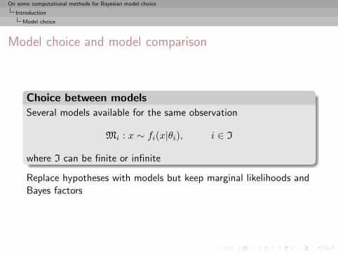
Model choice and model comparison
Choice between models
Several models available for the same observation
Mi : x ∼ fi(x|θi), i ∈ I
where I can be finite or infinite
Replace hypotheses with models but keep marginal likelihoods andBayes factors
On some computational methods for Bayesian model choice
Introduction
Model choice
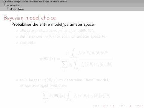
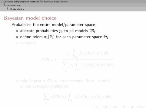
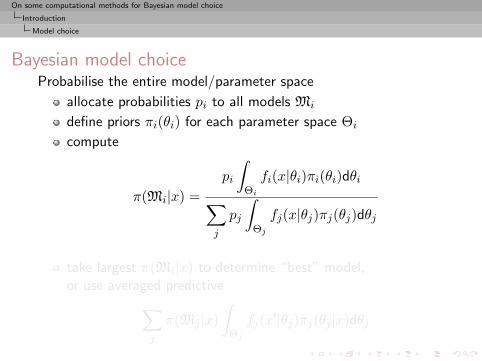
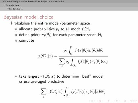
Bayesian model choiceProbabilise the entire model/parameter space
allocate probabilities pi to all models Mi
define priors πi(θi) for each parameter space Θi
compute
π(Mi|x) =pi
∫Θi
fi(x|θi)πi(θi)dθi∑j
pj
∫Θj
fj(x|θj)πj(θj)dθj
take largest π(Mi|x) to determine “best” model,or use averaged predictive∑
j
π(Mj |x)∫
Θj
fj(x′|θj)πj(θj |x)dθj
On some computational methods for Bayesian model choice
Introduction
Model choice
Bayesian model choiceProbabilise the entire model/parameter space
allocate probabilities pi to all models Mi
define priors πi(θi) for each parameter space Θi
compute
π(Mi|x) =pi
∫Θi
fi(x|θi)πi(θi)dθi∑j
pj
∫Θj
fj(x|θj)πj(θj)dθj
take largest π(Mi|x) to determine “best” model,or use averaged predictive∑
j
π(Mj |x)∫
Θj
fj(x′|θj)πj(θj |x)dθj

On some computational methods for Bayesian model choice
Introduction
Evidence
Evidence
All these problems end up with a similar quantity, the evidence
Zk =∫
Θk
πk(θk)Lk(θk) dθk,
aka the marginal likelihood.
On some computational methods for Bayesian model choice
Importance sampling solutions
Regular importance
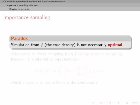
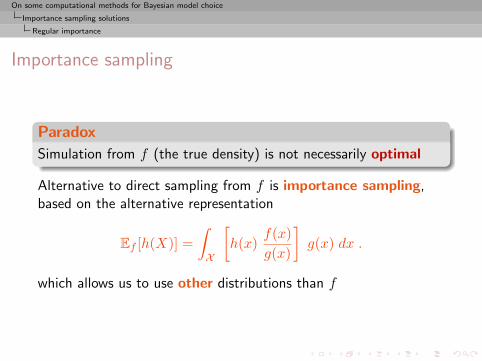
Importance sampling
Paradox
Simulation from f (the true density) is not necessarily optimal
Alternative to direct sampling from f is importance sampling,based on the alternative representation
Ef [h(X)] =∫X
[h(x)
f(x)g(x)
]g(x) dx .
which allows us to use other distributions than f
On some computational methods for Bayesian model choice
Importance sampling solutions
Regular importance
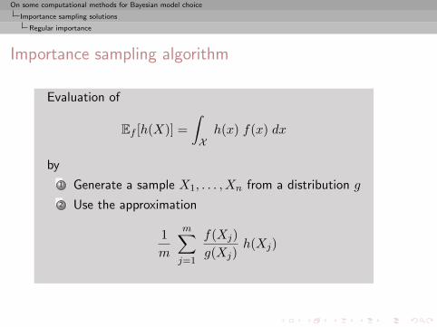
Importance sampling algorithm
Evaluation of
Ef [h(X)] =∫Xh(x) f(x) dx
by
1 Generate a sample X1, . . . , Xn from a distribution g
2 Use the approximation
1m
m∑j=1
f(Xj)g(Xj)
h(Xj)
On some computational methods for Bayesian model choice
Importance sampling solutions
Regular importance
Bayes factor approximation
When approximating the Bayes factor
B01 =
∫Θ0
f0(x|θ0)π0(θ0)dθ0∫Θ1
f1(x|θ1)π1(θ1)dθ1
use of importance functions $0 and $1 and
B01 =n−1
0
∑n0i=1 f0(x|θi0)π0(θi0)/$0(θi0)
n−11
∑n1i=1 f1(x|θi1)π1(θi1)/$1(θi1)
On some computational methods for Bayesian model choice
Importance sampling solutions
Regular importance
Bridge sampling
Special case:If
π1(θ1|x) ∝ π1(θ1|x)π2(θ2|x) ∝ π2(θ2|x)
live on the same space (Θ1 = Θ2), then
B12 ≈1n
n∑i=1
π1(θi|x)π2(θi|x)
θi ∼ π2(θ|x)
[Gelman & Meng, 1998; Chen, Shao & Ibrahim, 2000]
On some computational methods for Bayesian model choice
Importance sampling solutions
Regular importance
Bridge sampling variance
The bridge sampling estimator does poorly if
var(B12)B2
12
=1n
E
[(π1(θ)− π2(θ)
π2(θ)
)2]
is large, i.e. if π1 and π2 have little overlap...
On some computational methods for Bayesian model choice
Importance sampling solutions
Regular importance
Bridge sampling variance
The bridge sampling estimator does poorly if
var(B12)B2
12
=1n
E
[(π1(θ)− π2(θ)
π2(θ)
)2]
is large, i.e. if π1 and π2 have little overlap...
On some computational methods for Bayesian model choice
Importance sampling solutions
Regular importance
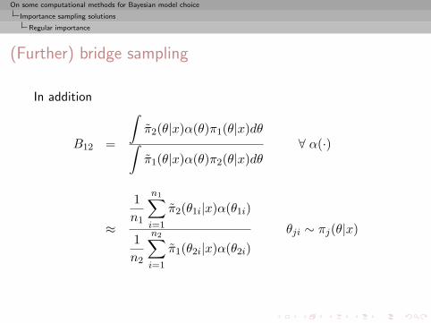
(Further) bridge sampling
In addition
B12 =
∫π2(θ|x)α(θ)π1(θ|x)dθ∫π1(θ|x)α(θ)π2(θ|x)dθ
∀ α(·)
≈
1n1
n1∑i=1
π2(θ1i|x)α(θ1i)
1n2
n2∑i=1
π1(θ2i|x)α(θ2i)θji ∼ πj(θ|x)
On some computational methods for Bayesian model choice
Importance sampling solutions
Regular importance
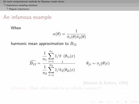
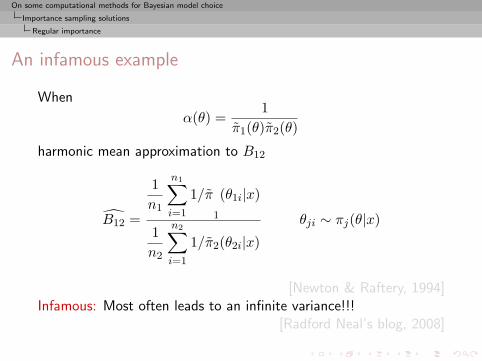
An infamous example
When
α(θ) =1
π1(θ)π2(θ)
harmonic mean approximation to B12
B12 =
1n1
n1∑i=1
1/π1
(θ1i|x)
1n2
n2∑i=1
1/π2(θ2i|x)
θji ∼ πj(θ|x)
[Newton & Raftery, 1994]Infamous: Most often leads to an infinite variance!!!
[Radford Neal’s blog, 2008]
On some computational methods for Bayesian model choice
Importance sampling solutions
Regular importance
An infamous example
When
α(θ) =1
π1(θ)π2(θ)
harmonic mean approximation to B12
B12 =
1n1
n1∑i=1
1/π1
(θ1i|x)
1n2
n2∑i=1
1/π2(θ2i|x)
θji ∼ πj(θ|x)
[Newton & Raftery, 1994]Infamous: Most often leads to an infinite variance!!!
[Radford Neal’s blog, 2008]

On some computational methods for Bayesian model choice
Importance sampling solutions
Regular importance
“The Worst Monte Carlo Method Ever”
“The good news is that the Law of Large Numbers guarantees thatthis estimator is consistent ie, it will very likely be very close to thecorrect answer if you use a sufficiently large number of points fromthe posterior distribution.The bad news is that the number of points required for thisestimator to get close to the right answer will often be greaterthan the number of atoms in the observable universe. The evenworse news is that itws easy for people to not realize this, and tonaively accept estimates that are nowhere close to the correctvalue of the marginal likelihood.”
[Radford Neal’s blog, Aug. 23, 2008]
On some computational methods for Bayesian model choice
Importance sampling solutions
Regular importance
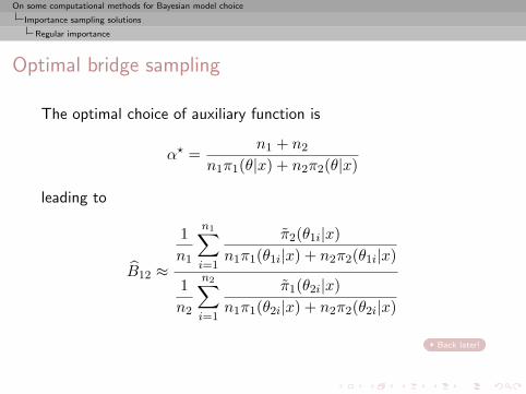
Optimal bridge sampling
The optimal choice of auxiliary function is
α? =n1 + n2
n1π1(θ|x) + n2π2(θ|x)
leading to
B12 ≈
1n1
n1∑i=1
π2(θ1i|x)n1π1(θ1i|x) + n2π2(θ1i|x)
1n2
n2∑i=1
π1(θ2i|x)n1π1(θ2i|x) + n2π2(θ2i|x)
Back later!
On some computational methods for Bayesian model choice
Importance sampling solutions
Regular importance
Optimal bridge sampling (2)
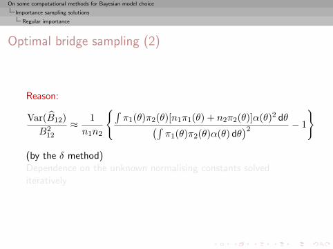
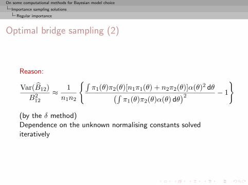
Reason:
Var(B12)B2
12
≈ 1n1n2
{∫π1(θ)π2(θ)[n1π1(θ) + n2π2(θ)]α(θ)2 dθ(∫
π1(θ)π2(θ)α(θ) dθ)2 − 1
}
(by the δ method)Dependence on the unknown normalising constants solvediteratively
On some computational methods for Bayesian model choice
Importance sampling solutions
Regular importance
Optimal bridge sampling (2)
Reason:
Var(B12)B2
12
≈ 1n1n2
{∫π1(θ)π2(θ)[n1π1(θ) + n2π2(θ)]α(θ)2 dθ(∫
π1(θ)π2(θ)α(θ) dθ)2 − 1
}
(by the δ method)Dependence on the unknown normalising constants solvediteratively
On some computational methods for Bayesian model choice
Importance sampling solutions
Regular importance
Ratio importance sampling
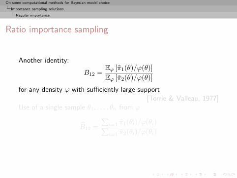
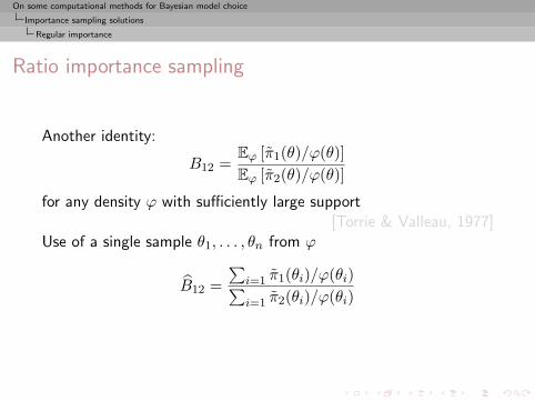
Another identity:
B12 =Eϕ [π1(θ)/ϕ(θ)]Eϕ [π2(θ)/ϕ(θ)]
for any density ϕ with sufficiently large support[Torrie & Valleau, 1977]
Use of a single sample θ1, . . . , θn from ϕ
B12 =∑
i=1 π1(θi)/ϕ(θi)∑i=1 π2(θi)/ϕ(θi)
On some computational methods for Bayesian model choice
Importance sampling solutions
Regular importance
Ratio importance sampling
Another identity:
B12 =Eϕ [π1(θ)/ϕ(θ)]Eϕ [π2(θ)/ϕ(θ)]
for any density ϕ with sufficiently large support[Torrie & Valleau, 1977]
Use of a single sample θ1, . . . , θn from ϕ
B12 =∑
i=1 π1(θi)/ϕ(θi)∑i=1 π2(θi)/ϕ(θi)
On some computational methods for Bayesian model choice
Importance sampling solutions
Regular importance
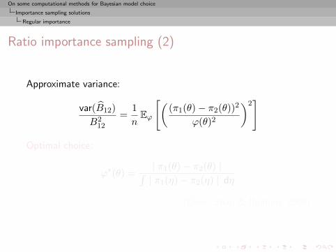
Ratio importance sampling (2)
Approximate variance:
var(B12)B2
12
=1n
Eϕ
[((π1(θ)− π2(θ))2
ϕ(θ)2
)2]
Optimal choice:
ϕ∗(θ) =| π1(θ)− π2(θ) |∫| π1(η)− π2(η) | dη
[Chen, Shao & Ibrahim, 2000]
On some computational methods for Bayesian model choice
Importance sampling solutions
Regular importance
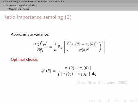
Ratio importance sampling (2)
Approximate variance:
var(B12)B2
12
=1n
Eϕ
[((π1(θ)− π2(θ))2
ϕ(θ)2
)2]
Optimal choice:
ϕ∗(θ) =| π1(θ)− π2(θ) |∫| π1(η)− π2(η) | dη
[Chen, Shao & Ibrahim, 2000]
On some computational methods for Bayesian model choice
Importance sampling solutions
Regular importance
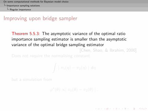
Improving upon bridge sampler
Theorem 5.5.3: The asymptotic variance of the optimal ratioimportance sampling estimator is smaller than the asymptoticvariance of the optimal bridge sampling estimator
[Chen, Shao, & Ibrahim, 2000]Does not require the normalising constant∫
| π1(η)− π2(η) | dη
but a simulation from
ϕ∗(θ) ∝| π1(θ)− π2(θ) | .
On some computational methods for Bayesian model choice
Importance sampling solutions
Regular importance
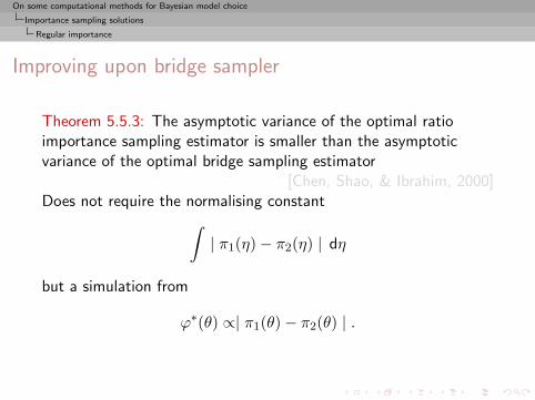
Improving upon bridge sampler
Theorem 5.5.3: The asymptotic variance of the optimal ratioimportance sampling estimator is smaller than the asymptoticvariance of the optimal bridge sampling estimator
[Chen, Shao, & Ibrahim, 2000]Does not require the normalising constant∫
| π1(η)− π2(η) | dη
but a simulation from
ϕ∗(θ) ∝| π1(θ)− π2(θ) | .

On some computational methods for Bayesian model choice
Importance sampling solutions
Varying dimensions
Generalisation to point null situations
When
B12 =
∫Θ1
π1(θ1)dθ1∫Θ2
π2(θ2)dθ2
and Θ2 = Θ1 ×Ψ, we get θ2 = (θ1, ψ) and
B12 = Eπ2
[π1(θ1)ω(ψ|θ1)π2(θ1, ψ)
]holds for any conditional density ω(ψ|θ1).
On some computational methods for Bayesian model choice
Importance sampling solutions
Varying dimensions
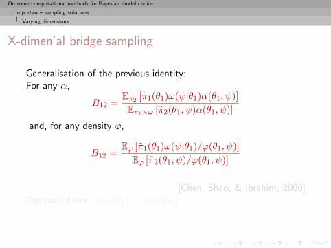
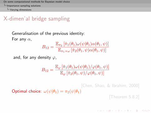
X-dimen’al bridge sampling
Generalisation of the previous identity:For any α,
B12 =Eπ2 [π1(θ1)ω(ψ|θ1)α(θ1, ψ)]Eπ1×ω [π2(θ1, ψ)α(θ1, ψ)]
and, for any density ϕ,
B12 =Eϕ [π1(θ1)ω(ψ|θ1)/ϕ(θ1, ψ)]
Eϕ [π2(θ1, ψ)/ϕ(θ1, ψ)]
[Chen, Shao, & Ibrahim, 2000]Optimal choice: ω(ψ|θ1) = π2(ψ|θ1)
[Theorem 5.8.2]
On some computational methods for Bayesian model choice
Importance sampling solutions
Varying dimensions
X-dimen’al bridge sampling
Generalisation of the previous identity:For any α,
B12 =Eπ2 [π1(θ1)ω(ψ|θ1)α(θ1, ψ)]Eπ1×ω [π2(θ1, ψ)α(θ1, ψ)]
and, for any density ϕ,
B12 =Eϕ [π1(θ1)ω(ψ|θ1)/ϕ(θ1, ψ)]
Eϕ [π2(θ1, ψ)/ϕ(θ1, ψ)]
[Chen, Shao, & Ibrahim, 2000]Optimal choice: ω(ψ|θ1) = π2(ψ|θ1)
[Theorem 5.8.2]

On some computational methods for Bayesian model choice
Importance sampling solutions
Harmonic means
Approximating Zk from a posterior sample
Use of the [harmonic mean] identity
Eπk[
ϕ(θk)πk(θk)Lk(θk)
∣∣∣∣x] =∫
ϕ(θk)πk(θk)Lk(θk)
πk(θk)Lk(θk)Zk
dθk =1Zk
no matter what the proposal ϕ(·) is.[Gelfand & Dey, 1994; Bartolucci et al., 2006]
Direct exploitation of the MCMC outputRB-RJ
On some computational methods for Bayesian model choice
Importance sampling solutions
Harmonic means
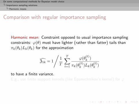
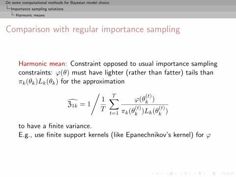
Comparison with regular importance sampling
Harmonic mean: Constraint opposed to usual importance samplingconstraints: ϕ(θ) must have lighter (rather than fatter) tails thanπk(θk)Lk(θk) for the approximation
Z1k = 1
/1T
T∑t=1
ϕ(θ(t)k )
πk(θ(t)k )Lk(θ
(t)k )
to have a finite variance.E.g., use finite support kernels (like Epanechnikov’s kernel) for ϕ
On some computational methods for Bayesian model choice
Importance sampling solutions
Harmonic means
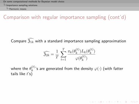
Comparison with regular importance sampling (cont’d)
Compare Z1k with a standard importance sampling approximation
Z2k =1T
T∑t=1
πk(θ(t)k )Lk(θ
(t)k )
ϕ(θ(t)k )
where the θ(t)k ’s are generated from the density ϕ(·) (with fatter
tails like t’s)
On some computational methods for Bayesian model choice
Importance sampling solutions
Harmonic means
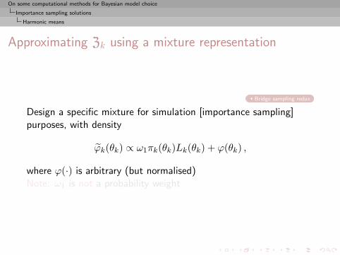
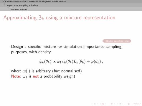
Approximating Zk using a mixture representation
Bridge sampling redux
Design a specific mixture for simulation [importance sampling]purposes, with density
ϕk(θk) ∝ ω1πk(θk)Lk(θk) + ϕ(θk) ,
where ϕ(·) is arbitrary (but normalised)Note: ω1 is not a probability weight
On some computational methods for Bayesian model choice
Importance sampling solutions
Harmonic means
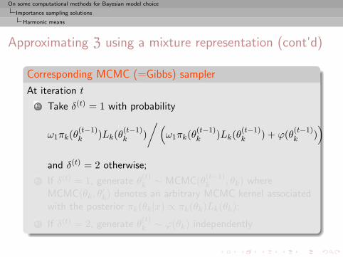
Approximating Z using a mixture representation (cont’d)
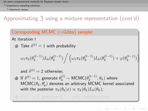
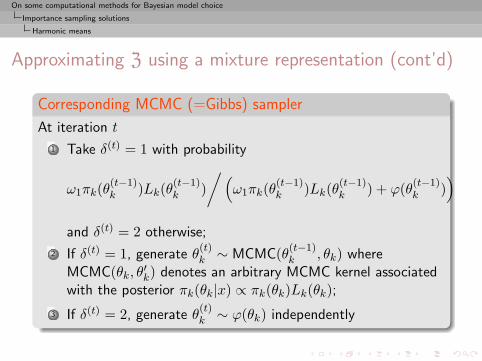
Corresponding MCMC (=Gibbs) sampler
At iteration t
1 Take δ(t) = 1 with probability
ω1πk(θ(t−1)k )Lk(θ
(t−1)k )
/(ω1πk(θ
(t−1)k )Lk(θ
(t−1)k ) + ϕ(θ(t−1)
k ))
and δ(t) = 2 otherwise;
2 If δ(t) = 1, generate θ(t)k ∼ MCMC(θ(t−1)
k , θk) whereMCMC(θk, θ′k) denotes an arbitrary MCMC kernel associatedwith the posterior πk(θk|x) ∝ πk(θk)Lk(θk);
3 If δ(t) = 2, generate θ(t)k ∼ ϕ(θk) independently
On some computational methods for Bayesian model choice
Importance sampling solutions
Harmonic means
Approximating Z using a mixture representation (cont’d)
Corresponding MCMC (=Gibbs) sampler
At iteration t
1 Take δ(t) = 1 with probability
ω1πk(θ(t−1)k )Lk(θ
(t−1)k )
/(ω1πk(θ
(t−1)k )Lk(θ
(t−1)k ) + ϕ(θ(t−1)
k ))
and δ(t) = 2 otherwise;
2 If δ(t) = 1, generate θ(t)k ∼ MCMC(θ(t−1)
k , θk) whereMCMC(θk, θ′k) denotes an arbitrary MCMC kernel associatedwith the posterior πk(θk|x) ∝ πk(θk)Lk(θk);
3 If δ(t) = 2, generate θ(t)k ∼ ϕ(θk) independently
On some computational methods for Bayesian model choice
Importance sampling solutions
Harmonic means
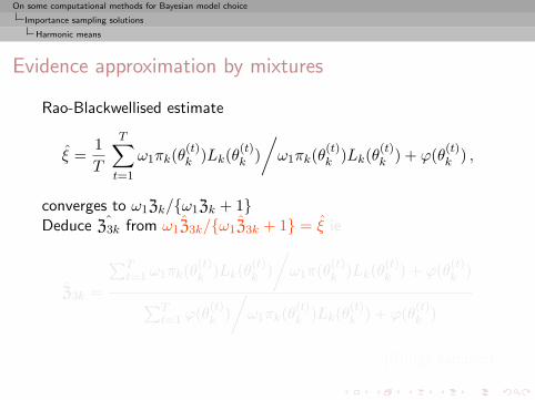
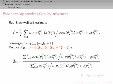
Evidence approximation by mixtures
Rao-Blackwellised estimate
ξ =1T
T∑t=1
ω1πk(θ(t)k )Lk(θ
(t)k )/ω1πk(θ
(t)k )Lk(θ
(t)k ) + ϕ(θ(t)
k ) ,
converges to ω1Zk/{ω1Zk + 1}Deduce Z3k from ω1Z3k/{ω1Z3k + 1} = ξ ie
Z3k =
∑Tt=1 ω1πk(θ
(t)k )Lk(θ
(t)k )/ω1π(θ(t)
k )Lk(θ(t)k ) + ϕ(θ(t)
k )
∑Tt=1 ϕ(θ(t)
k )/ω1πk(θ
(t)k )Lk(θ
(t)k ) + ϕ(θ(t)
k )
[Bridge sampler]
On some computational methods for Bayesian model choice
Importance sampling solutions
Harmonic means
Evidence approximation by mixtures
Rao-Blackwellised estimate
ξ =1T
T∑t=1
ω1πk(θ(t)k )Lk(θ
(t)k )/ω1πk(θ
(t)k )Lk(θ
(t)k ) + ϕ(θ(t)
k ) ,
converges to ω1Zk/{ω1Zk + 1}Deduce Z3k from ω1Z3k/{ω1Z3k + 1} = ξ ie
Z3k =
∑Tt=1 ω1πk(θ
(t)k )Lk(θ
(t)k )/ω1π(θ(t)
k )Lk(θ(t)k ) + ϕ(θ(t)
k )
∑Tt=1 ϕ(θ(t)
k )/ω1πk(θ
(t)k )Lk(θ
(t)k ) + ϕ(θ(t)
k )
[Bridge sampler]
On some computational methods for Bayesian model choice
Importance sampling solutions
Chib’s solution
Chib’s representation
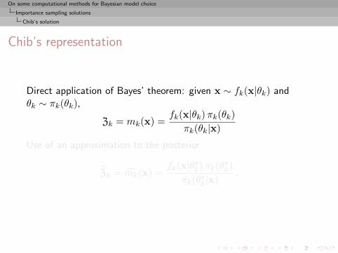
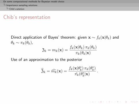
Direct application of Bayes’ theorem: given x ∼ fk(x|θk) andθk ∼ πk(θk),
Zk = mk(x) =fk(x|θk)πk(θk)
πk(θk|x)
Use of an approximation to the posterior
Zk = mk(x) =fk(x|θ∗k)πk(θ∗k)
πk(θ∗k|x).
On some computational methods for Bayesian model choice
Importance sampling solutions
Chib’s solution
Chib’s representation
Direct application of Bayes’ theorem: given x ∼ fk(x|θk) andθk ∼ πk(θk),
Zk = mk(x) =fk(x|θk)πk(θk)
πk(θk|x)
Use of an approximation to the posterior
Zk = mk(x) =fk(x|θ∗k)πk(θ∗k)
πk(θ∗k|x).

On some computational methods for Bayesian model choice
Importance sampling solutions
Chib’s solution
Case of latent variables
For missing variable z as in mixture models, natural Rao-Blackwellestimate
πk(θ∗k|x) =1T
T∑t=1
πk(θ∗k|x, z(t)k ) ,
where the z(t)k ’s are Gibbs sampled latent variables
On some computational methods for Bayesian model choice
Importance sampling solutions
Chib’s solution
Label switching
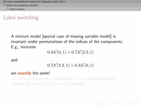
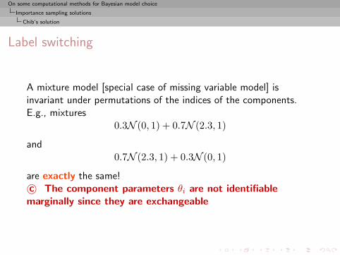
A mixture model [special case of missing variable model] isinvariant under permutations of the indices of the components.E.g., mixtures
0.3N (0, 1) + 0.7N (2.3, 1)
and0.7N (2.3, 1) + 0.3N (0, 1)
are exactly the same!c© The component parameters θi are not identifiablemarginally since they are exchangeable
On some computational methods for Bayesian model choice
Importance sampling solutions
Chib’s solution
Label switching
A mixture model [special case of missing variable model] isinvariant under permutations of the indices of the components.E.g., mixtures
0.3N (0, 1) + 0.7N (2.3, 1)
and0.7N (2.3, 1) + 0.3N (0, 1)
are exactly the same!c© The component parameters θi are not identifiablemarginally since they are exchangeable

On some computational methods for Bayesian model choice
Importance sampling solutions
Chib’s solution
Connected difficulties
1 Number of modes of the likelihood of order O(k!):c© Maximization and even [MCMC] exploration of the
posterior surface harder
2 Under exchangeable priors on (θ,p) [prior invariant underpermutation of the indices], all posterior marginals areidentical:c© Posterior expectation of θ1 equal to posterior expectation
of θ2
On some computational methods for Bayesian model choice
Importance sampling solutions
Chib’s solution
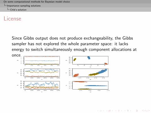
License
Since Gibbs output does not produce exchangeability, the Gibbssampler has not explored the whole parameter space: it lacksenergy to switch simultaneously enough component allocations atonce
0 100 200 300 400 500
−10
12
3
n
µ i
−1 0 1 2 3
0.20.3
0.40.5
µi
p i
0 100 200 300 400 500
0.20.3
0.40.5
n
p i
0.2 0.3 0.4 0.5
0.40.6
0.81.0
pi
σ i
0 100 200 300 400 500
0.40.6
0.81.0
n
σ i
0.4 0.6 0.8 1.0
−10
12
3
σi
µ i

On some computational methods for Bayesian model choice
Importance sampling solutions
Chib’s solution
Label switching paradox
We should observe the exchangeability of the components [labelswitching] to conclude about convergence of the Gibbs sampler.If we observe it, then we do not know how to estimate theparameters.If we do not, then we are uncertain about the convergence!!!
On some computational methods for Bayesian model choice
Importance sampling solutions
Chib’s solution
Compensation for label switching
For mixture models, z(t)k usually fails to visit all configurations in a
balanced way, despite the symmetry predicted by the theory
πk(θk|x) = πk(σ(θk)|x) =1k!
∑σ∈S
πk(σ(θk)|x)
for all σ’s in Sk, set of all permutations of {1, . . . , k}.Consequences on numerical approximation, biased by an order k!Recover the theoretical symmetry by using
πk(θ∗k|x) =1T k!
∑σ∈Sk
T∑t=1
πk(σ(θ∗k)|x, z(t)k ) .
[Berkhof, Mechelen, & Gelman, 2003]

On some computational methods for Bayesian model choice
Importance sampling solutions
Chib’s solution
Galaxy dataset
n = 82 galaxies as a mixture of k normal distributions with bothmean and variance unknown.
[Roeder, 1992]Average density
data
Rel
ativ
e F
requ
ency
−2 −1 0 1 2 3
0.0
0.2
0.4
0.6
0.8
On some computational methods for Bayesian model choice
Importance sampling solutions
Chib’s solution
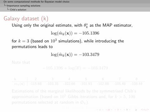
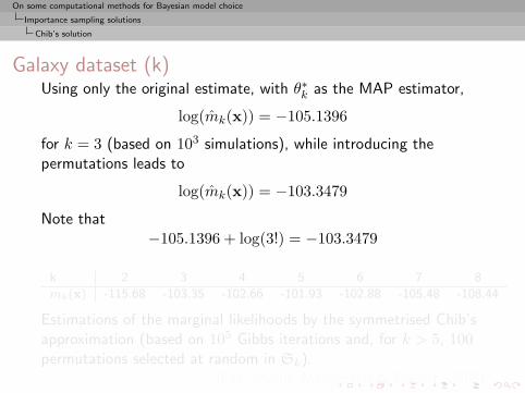
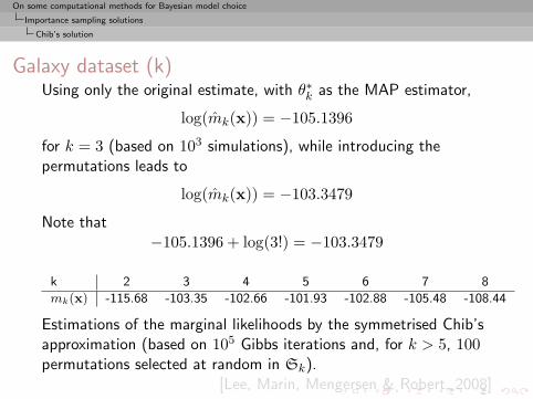
Galaxy dataset (k)Using only the original estimate, with θ∗k as the MAP estimator,
log(mk(x)) = −105.1396
for k = 3 (based on 103 simulations), while introducing thepermutations leads to
log(mk(x)) = −103.3479
Note that−105.1396 + log(3!) = −103.3479
k 2 3 4 5 6 7 8
mk(x) -115.68 -103.35 -102.66 -101.93 -102.88 -105.48 -108.44
Estimations of the marginal likelihoods by the symmetrised Chib’sapproximation (based on 105 Gibbs iterations and, for k > 5, 100permutations selected at random in Sk).
[Lee, Marin, Mengersen & Robert, 2008]
On some computational methods for Bayesian model choice
Importance sampling solutions
Chib’s solution
Galaxy dataset (k)Using only the original estimate, with θ∗k as the MAP estimator,
log(mk(x)) = −105.1396
for k = 3 (based on 103 simulations), while introducing thepermutations leads to
log(mk(x)) = −103.3479
Note that−105.1396 + log(3!) = −103.3479
k 2 3 4 5 6 7 8
mk(x) -115.68 -103.35 -102.66 -101.93 -102.88 -105.48 -108.44
Estimations of the marginal likelihoods by the symmetrised Chib’sapproximation (based on 105 Gibbs iterations and, for k > 5, 100permutations selected at random in Sk).
[Lee, Marin, Mengersen & Robert, 2008]
On some computational methods for Bayesian model choice
Cross-model solutions
Variable selection
Bayesian variable selection
Regression setting: one dependent random variable y and a set{x1, . . . , xk} of k explanatory variables.
Question: Are all xi’s involved in the regression?
Assumption: every subset {i1, . . . , iq} of q (0 ≤ q ≤ k)explanatory variables, {1n, xi1 , . . . , xiq}, is a proper set ofexplanatory variables for the regression of y [intercept included inevery corresponding model]
Computational issue
2k models in competition...
On some computational methods for Bayesian model choice
Cross-model solutions
Variable selection
Model notations
1
X =[1n x1 · · · xk
]is the matrix containing 1n and all the k potential predictorvariables
2 Each model Mγ associated with binary indicator vectorγ ∈ Γ = {0, 1}k where γi = 1 means that the variable xi isincluded in the model Mγ
3 qγ = 1Tnγ number of variables included in the model Mγ
4 t1(γ) and t0(γ) indices of variables included in the model andindices of variables not included in the model

On some computational methods for Bayesian model choice
Cross-model solutions
Variable selection
Model indicators
For β ∈ Rk+1 and X, we define βγ as the subvector
βγ =(β0, (βi)i∈t1(γ)
)and Xγ as the submatrix of X where only the column 1n and thecolumns in t1(γ) have been left.
On some computational methods for Bayesian model choice
Cross-model solutions
Variable selection
Models in competition
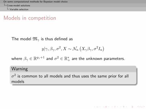
The model Mγ is thus defined as
y|γ, βγ , σ2, X ∼ Nn(Xγβγ , σ
2In)
where βγ ∈ Rqγ+1 and σ2 ∈ R∗+ are the unknown parameters.
Warning
σ2 is common to all models and thus uses the same prior for allmodels
On some computational methods for Bayesian model choice
Cross-model solutions
Variable selection
Models in competition
The model Mγ is thus defined as
y|γ, βγ , σ2, X ∼ Nn(Xγβγ , σ
2In)
where βγ ∈ Rqγ+1 and σ2 ∈ R∗+ are the unknown parameters.
Warning
σ2 is common to all models and thus uses the same prior for allmodels

On some computational methods for Bayesian model choice
Cross-model solutions
Variable selection
Informative G-prior
Many (2k) models in competition: we cannot expect a practitionerto specify a prior on every Mγ in a completely subjective andautonomous manner.
Shortcut: We derive all priors from a single global prior associatedwith the so-called full model that corresponds to γ = (1, . . . , 1).
On some computational methods for Bayesian model choice
Cross-model solutions
Variable selection
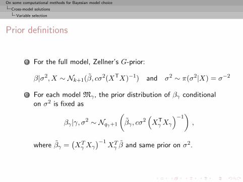
Prior definitions
(i) For the full model, Zellner’s G-prior:
β|σ2, X ∼ Nk+1(β, cσ2(XTX)−1) and σ2 ∼ π(σ2|X) = σ−2
(ii) For each model Mγ , the prior distribution of βγ conditionalon σ2 is fixed as
βγ |γ, σ2 ∼ Nqγ+1
(βγ , cσ
2(XTγ Xγ
)−1),
where βγ =(XTγ Xγ
)−1XTγ β and same prior on σ2.
On some computational methods for Bayesian model choice
Cross-model solutions
Variable selection
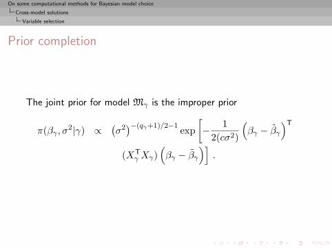
Prior completion
The joint prior for model Mγ is the improper prior
π(βγ , σ2|γ) ∝(σ2)−(qγ+1)/2−1 exp
[− 1
2(cσ2)
(βγ − βγ
)T
(XTγ Xγ)
(βγ − βγ
)].
On some computational methods for Bayesian model choice
Cross-model solutions
Variable selection
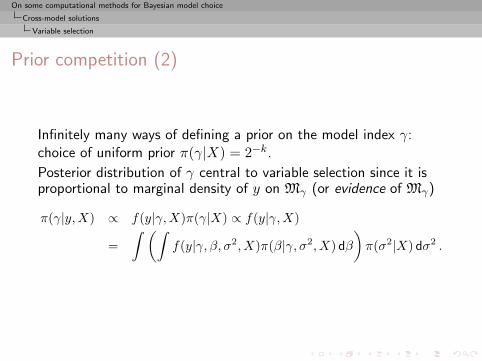
Prior competition (2)
Infinitely many ways of defining a prior on the model index γ:choice of uniform prior π(γ|X) = 2−k.
Posterior distribution of γ central to variable selection since it isproportional to marginal density of y on Mγ (or evidence of Mγ)
π(γ|y,X) ∝ f(y|γ,X)π(γ|X) ∝ f(y|γ,X)
=∫ (∫
f(y|γ, β, σ2, X)π(β|γ, σ2, X) dβ
)π(σ2|X) dσ2 .
On some computational methods for Bayesian model choice
Cross-model solutions
Variable selection
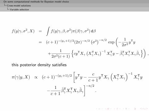
f(y|γ, σ2, X) =∫f(y|γ, β, σ2)π(β|γ, σ2) dβ
= (c+ 1)−(qγ+1)/2(2π)−n/2(σ2)−n/2
exp(− 1
2σ2yTy
+1
2σ2(c+ 1)
{cyTXγ
(XTγXγ
)−1XTγ y − βT
γXTγXγ βγ
}),
this posterior density satisfies
π(γ|y,X) ∝ (c+ 1)−(qγ+1)/2
[yTy − c
c+ 1yTXγ
(XTγ Xγ
)−1XTγ y
− 1c+ 1
βTγX
Tγ Xγ βγ
]−n/2.
On some computational methods for Bayesian model choice
Cross-model solutions
Variable selection
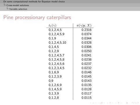
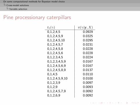
Pine processionary caterpillars
t1(γ) π(γ|y, X)
0,1,2,4,5 0.23160,1,2,4,5,9 0.03740,1,9 0.03440,1,2,4,5,10 0.03280,1,4,5 0.03060,1,2,9 0.02500,1,2,4,5,7 0.02410,1,2,4,5,8 0.02380,1,2,4,5,6 0.02370,1,2,3,4,5 0.02320,1,6,9 0.01460,1,2,3,9 0.01450,9 0.01430,1,2,6,9 0.01350,1,4,5,9 0.01280,1,3,9 0.01170,1,2,8 0.0115
On some computational methods for Bayesian model choice
Cross-model solutions
Variable selection
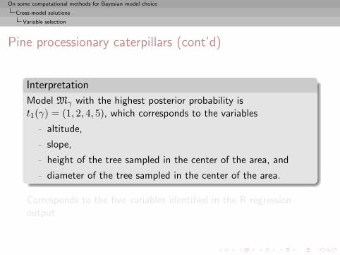
Pine processionary caterpillars (cont’d)
Interpretation
Model Mγ with the highest posterior probability ist1(γ) = (1, 2, 4, 5), which corresponds to the variables
- altitude,
- slope,
- height of the tree sampled in the center of the area, and
- diameter of the tree sampled in the center of the area.
Corresponds to the five variables identified in the R regressionoutput
On some computational methods for Bayesian model choice
Cross-model solutions
Variable selection
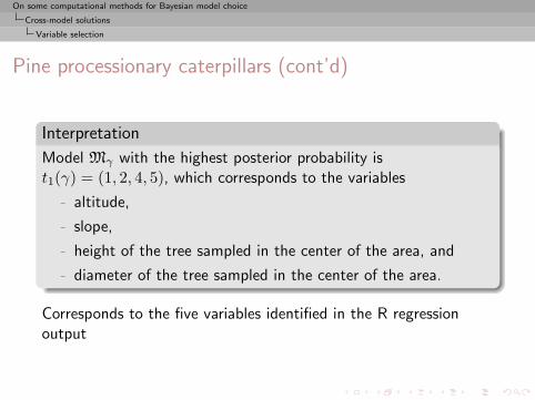
Pine processionary caterpillars (cont’d)
Interpretation
Model Mγ with the highest posterior probability ist1(γ) = (1, 2, 4, 5), which corresponds to the variables
- altitude,
- slope,
- height of the tree sampled in the center of the area, and
- diameter of the tree sampled in the center of the area.
Corresponds to the five variables identified in the R regressionoutput

On some computational methods for Bayesian model choice
Cross-model solutions
Variable selection
Noninformative extension
For Zellner noninformative prior with π(c) = 1/c, we have
π(γ|y,X) ∝∞∑c=1
c−1(c+ 1)−(qγ+1)/2[yTy−
c
c+ 1yTXγ
(XTγ Xγ
)−1XTγ y
]−n/2.
On some computational methods for Bayesian model choice
Cross-model solutions
Variable selection
Pine processionary caterpillars
t1(γ) π(γ|y, X)
0,1,2,4,5 0.09290,1,2,4,5,9 0.03250,1,2,4,5,10 0.02950,1,2,4,5,7 0.02310,1,2,4,5,8 0.02280,1,2,4,5,6 0.02280,1,2,3,4,5 0.02240,1,2,3,4,5,9 0.01670,1,2,4,5,6,9 0.01670,1,2,4,5,8,9 0.01370,1,4,5 0.01100,1,2,4,5,9,10 0.01000,1,2,3,9 0.00970,1,2,9 0.00930,1,2,4,5,7,9 0.00920,1,2,6,9 0.0092
On some computational methods for Bayesian model choice
Cross-model solutions
Variable selection
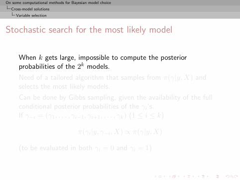
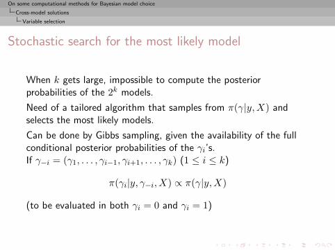
Stochastic search for the most likely model
When k gets large, impossible to compute the posteriorprobabilities of the 2k models.
Need of a tailored algorithm that samples from π(γ|y,X) andselects the most likely models.
Can be done by Gibbs sampling, given the availability of the fullconditional posterior probabilities of the γi’s.If γ−i = (γ1, . . . , γi−1, γi+1, . . . , γk) (1 ≤ i ≤ k)
π(γi|y, γ−i, X) ∝ π(γ|y,X)
(to be evaluated in both γi = 0 and γi = 1)
On some computational methods for Bayesian model choice
Cross-model solutions
Variable selection
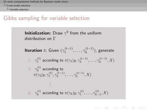
Gibbs sampling for variable selection
Initialization: Draw γ0 from the uniformdistribution on Γ
Iteration t: Given (γ(t−1)1 , . . . , γ
(t−1)k ), generate
1. γ(t)1 according to π(γ1|y, γ(t−1)
2 , . . . , γ(t−1)k , X)
2. γ(t)2 according to
π(γ2|y, γ(t)1 , γ
(t−1)3 , . . . , γ
(t−1)k , X)
...
p. γ(t)k according to π(γk|y, γ(t)
1 , . . . , γ(t)k−1, X)
On some computational methods for Bayesian model choice
Cross-model solutions
Variable selection
MCMC interpretation
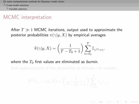
After T � 1 MCMC iterations, output used to approximate theposterior probabilities π(γ|y,X) by empirical averages
π(γ|y,X) =(
1T − T0 + 1
) T∑t=T0
Iγ(t)=γ .
where the T0 first values are eliminated as burnin.
And approximation of the probability to include i-th variable,
P π(γi = 1|y,X) =(
1T − T0 + 1
) T∑t=T0
Iγ(t)i =1
.
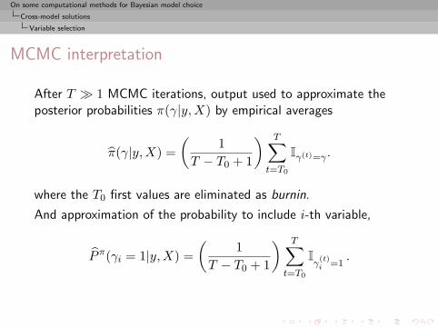
On some computational methods for Bayesian model choice
Cross-model solutions
Variable selection
MCMC interpretation
After T � 1 MCMC iterations, output used to approximate theposterior probabilities π(γ|y,X) by empirical averages
π(γ|y,X) =(
1T − T0 + 1
) T∑t=T0
Iγ(t)=γ .
where the T0 first values are eliminated as burnin.
And approximation of the probability to include i-th variable,
P π(γi = 1|y,X) =(
1T − T0 + 1
) T∑t=T0
Iγ(t)i =1
.
On some computational methods for Bayesian model choice
Cross-model solutions
Variable selection
Pine processionary caterpillars
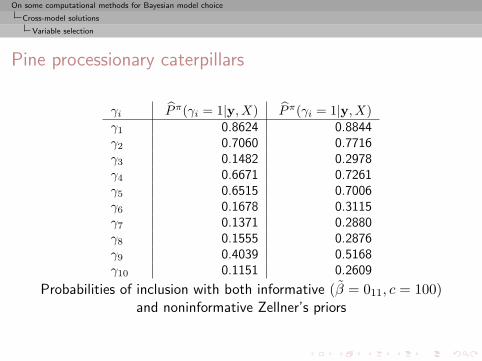
γi Pπ(γi = 1|y, X) Pπ(γi = 1|y, X)γ1 0.8624 0.8844γ2 0.7060 0.7716γ3 0.1482 0.2978γ4 0.6671 0.7261γ5 0.6515 0.7006γ6 0.1678 0.3115γ7 0.1371 0.2880γ8 0.1555 0.2876γ9 0.4039 0.5168γ10 0.1151 0.2609
Probabilities of inclusion with both informative (β = 011, c = 100)and noninformative Zellner’s priors

On some computational methods for Bayesian model choice
Cross-model solutions
Reversible jump
Reversible jump
Idea: Set up a proper measure–theoretic framework for designingmoves between models Mk
[Green, 1995]Create a reversible kernel K on H =
⋃k{k} ×Θk such that∫
A
∫B
K(x, dy)π(x)dx =∫B
∫A
K(y, dx)π(y)dy
for the invariant density π [x is of the form (k, θ(k))]
On some computational methods for Bayesian model choice
Cross-model solutions
Reversible jump
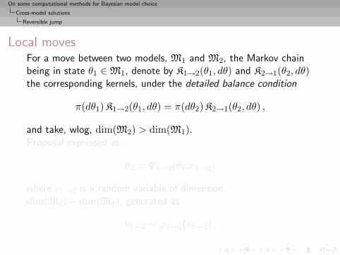
Local movesFor a move between two models, M1 and M2, the Markov chainbeing in state θ1 ∈M1, denote by K1→2(θ1, dθ) and K2→1(θ2, dθ)the corresponding kernels, under the detailed balance condition
π(dθ1) K1→2(θ1, dθ) = π(dθ2) K2→1(θ2, dθ) ,
and take, wlog, dim(M2) > dim(M1).Proposal expressed as
θ2 = Ψ1→2(θ1, v1→2)
where v1→2 is a random variable of dimensiondim(M2)− dim(M1), generated as
v1→2 ∼ ϕ1→2(v1→2) .
On some computational methods for Bayesian model choice
Cross-model solutions
Reversible jump
Local movesFor a move between two models, M1 and M2, the Markov chainbeing in state θ1 ∈M1, denote by K1→2(θ1, dθ) and K2→1(θ2, dθ)the corresponding kernels, under the detailed balance condition
π(dθ1) K1→2(θ1, dθ) = π(dθ2) K2→1(θ2, dθ) ,
and take, wlog, dim(M2) > dim(M1).Proposal expressed as
θ2 = Ψ1→2(θ1, v1→2)
where v1→2 is a random variable of dimensiondim(M2)− dim(M1), generated as
v1→2 ∼ ϕ1→2(v1→2) .

On some computational methods for Bayesian model choice
Cross-model solutions
Reversible jump
Local moves (2)
In this case, q1→2(θ1, dθ2) has density
ϕ1→2(v1→2)∣∣∣∣∂Ψ1→2(θ1, v1→2)
∂(θ1, v1→2)
∣∣∣∣−1
,
by the Jacobian rule.Reverse importance link
If probability $1→2 of choosing move to M2 while in M1,acceptance probability reduces to
α(θ1, v1→2) = 1∧ π(M2, θ2)$2→1
π(M1, θ1)$1→2 ϕ1→2(v1→2)
∣∣∣∣∂Ψ1→2(θ1, v1→2)∂(θ1, v1→2)
∣∣∣∣ .c©Difficult calibration
On some computational methods for Bayesian model choice
Cross-model solutions
Reversible jump
Interpretation
The representation puts us back in a fixed dimension setting:
M1 ×V1→2 and M2 in one-to-one relation.
reversibility imposes that θ1 is derived as
(θ1, v1→2) = Ψ−11→2(θ2)
appears like a regular Metropolis–Hastings move from thecouple (θ1, v1→2) to θ2 when stationary distributions areπ(M1, θ1)× ϕ1→2(v1→2) and π(M2, θ2), and when proposaldistribution is deterministic (??)
On some computational methods for Bayesian model choice
Cross-model solutions
Reversible jump
Pseudo-deterministic reasoning
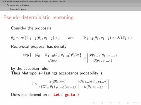
Consider the proposals
θ2 ∼ N (Ψ1→2(θ1, v1→2), ε) and Ψ1→2(θ1, v1→2) ∼ N (θ2, ε)
Reciprocal proposal has density
exp{−(θ2 −Ψ1→2(θ1, v1→2))2/2ε
}√
2πε×∣∣∣∣∂Ψ1→2(θ1, v1→2)
∂(θ1, v1→2)
∣∣∣∣by the Jacobian rule.Thus Metropolis–Hastings acceptance probability is
1 ∧ π(M2, θ2)π(M1, θ1)ϕ1→2(v1→2)
∣∣∣∣∂Ψ1→2(θ1, v1→2)∂(θ1, v1→2)
∣∣∣∣Does not depend on ε: Let ε go to 0
On some computational methods for Bayesian model choice
Cross-model solutions
Reversible jump
Pseudo-deterministic reasoning
Consider the proposals
θ2 ∼ N (Ψ1→2(θ1, v1→2), ε) and Ψ1→2(θ1, v1→2) ∼ N (θ2, ε)
Reciprocal proposal has density
exp{−(θ2 −Ψ1→2(θ1, v1→2))2/2ε
}√
2πε×∣∣∣∣∂Ψ1→2(θ1, v1→2)
∂(θ1, v1→2)
∣∣∣∣by the Jacobian rule.Thus Metropolis–Hastings acceptance probability is
1 ∧ π(M2, θ2)π(M1, θ1)ϕ1→2(v1→2)
∣∣∣∣∂Ψ1→2(θ1, v1→2)∂(θ1, v1→2)
∣∣∣∣Does not depend on ε: Let ε go to 0
On some computational methods for Bayesian model choice
Cross-model solutions
Reversible jump
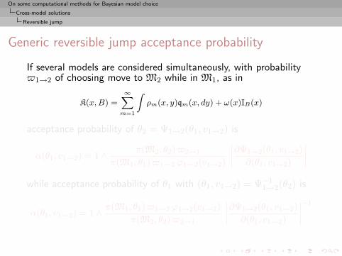
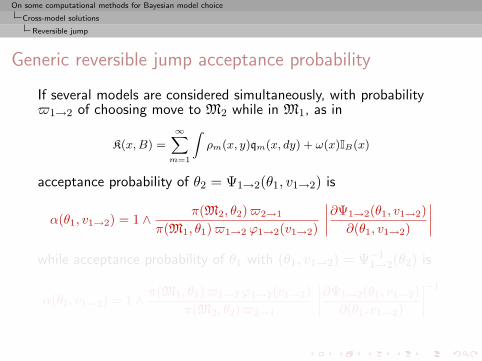
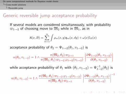
Generic reversible jump acceptance probability
If several models are considered simultaneously, with probability$1→2 of choosing move to M2 while in M1, as in
K(x,B) =∞Xm=1
Zρm(x, y)qm(x, dy) + ω(x)IB(x)
acceptance probability of θ2 = Ψ1→2(θ1, v1→2) is
α(θ1, v1→2) = 1 ∧ π(M2, θ2)$2→1
π(M1, θ1)$1→2 ϕ1→2(v1→2)
∣∣∣∣∂Ψ1→2(θ1, v1→2)∂(θ1, v1→2)
∣∣∣∣while acceptance probability of θ1 with (θ1, v1→2) = Ψ−1
1→2(θ2) is
α(θ1, v1→2) = 1 ∧ π(M1, θ1)$1→2 ϕ1→2(v1→2)π(M2, θ2)$2→1
∣∣∣∣∂Ψ1→2(θ1, v1→2)∂(θ1, v1→2)
∣∣∣∣−1
On some computational methods for Bayesian model choice
Cross-model solutions
Reversible jump
Green’s sampler
Algorithm
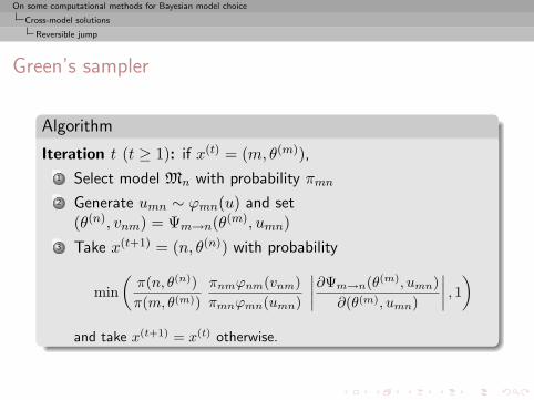
Iteration t (t ≥ 1): if x(t) = (m, θ(m)),
1 Select model Mn with probability πmn2 Generate umn ∼ ϕmn(u) and set
(θ(n), vnm) = Ψm→n(θ(m), umn)3 Take x(t+1) = (n, θ(n)) with probability
min(π(n, θ(n))π(m, θ(m))
πnmϕnm(vnm)πmnϕmn(umn)
∣∣∣∣∂Ψm→n(θ(m), umn)∂(θ(m), umn)
∣∣∣∣ , 1)and take x(t+1) = x(t) otherwise.
On some computational methods for Bayesian model choice
Cross-model solutions
Reversible jump
Mixture of normal distributions
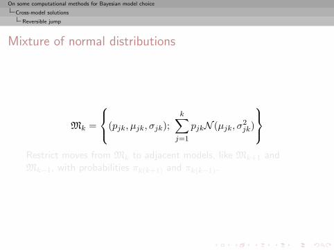
Mk =
(pjk, µjk, σjk);k∑j=1
pjkN (µjk, σ2jk)
Restrict moves from Mk to adjacent models, like Mk+1 andMk−1, with probabilities πk(k+1) and πk(k−1).
On some computational methods for Bayesian model choice
Cross-model solutions
Reversible jump
Mixture of normal distributions
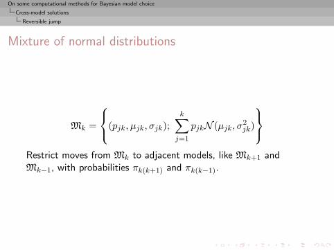
Mk =
(pjk, µjk, σjk);k∑j=1
pjkN (µjk, σ2jk)
Restrict moves from Mk to adjacent models, like Mk+1 andMk−1, with probabilities πk(k+1) and πk(k−1).
On some computational methods for Bayesian model choice
Cross-model solutions
Reversible jump
Mixture birth
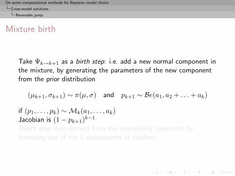
Take Ψk→k+1 as a birth step: i.e. add a new normal component inthe mixture, by generating the parameters of the new componentfrom the prior distribution
(µk+1, σk+1) ∼ π(µ, σ) and pk+1 ∼ Be(a1, a2 + . . .+ ak)
if (p1, . . . , pk) ∼Mk(a1, . . . , ak)Jacobian is (1− pk+1)k−1
Death step then derived from the reversibility constraint byremoving one of the k components at random.
On some computational methods for Bayesian model choice
Cross-model solutions
Reversible jump
Mixture birth
Take Ψk→k+1 as a birth step: i.e. add a new normal component inthe mixture, by generating the parameters of the new componentfrom the prior distribution
(µk+1, σk+1) ∼ π(µ, σ) and pk+1 ∼ Be(a1, a2 + . . .+ ak)
if (p1, . . . , pk) ∼Mk(a1, . . . , ak)Jacobian is (1− pk+1)k−1
Death step then derived from the reversibility constraint byremoving one of the k components at random.
On some computational methods for Bayesian model choice
Cross-model solutions
Reversible jump
Mixture acceptance probability
Birth acceptance probability
min(π(k+1)k
πk(k+1)
(k + 1)!(k + 1)k!
π(k + 1, θk+1)π(k, θk) (k + 1)ϕk(k+1)(uk(k+1))
, 1)
= min(π(k+1)k
πk(k+1)
%(k + 1)%(k)
`k+1(θk+1) (1− pk+1)k−1
`k(θk), 1),
where `k likelihood of the k component mixture model Mk and%(k) prior probability of model Mk.Combinatorial terms: there are (k + 1)! ways of defining a (k + 1)component mixture by adding one component, while, given a (k + 1)component mixture, there are (k+ 1) choices for a component to die and
then k! associated mixtures for the remaining components.

On some computational methods for Bayesian model choice
Cross-model solutions
Saturation schemes
AlternativeSaturation of the parameter space H =
⋃k{k} ×Θk by creating
θ = (θ1, . . . , θD)a model index Mpseudo-priors πj(θj |M = k) for j 6= k
[Carlin & Chib, 1995]Validation by
P(M = k|x) =∫P (M = k|x, θ)π(θ|x)dθ = Zk
where the (marginal) posterior is [not πk!]
π(θ|x) =D∑k=1
P(θ,M = k|x)
=D∑k=1
pk Zk πk(θk|x)∏j 6=k
πj(θj |M = k) .
On some computational methods for Bayesian model choice
Cross-model solutions
Saturation schemes
MCMC implementation
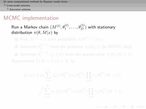
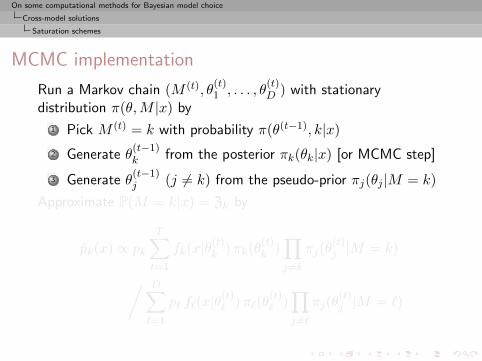
Run a Markov chain (M (t), θ(t)1 , . . . , θ
(t)D ) with stationary
distribution π(θ,M |x) by
1 Pick M (t) = k with probability π(θ(t−1), k|x)
2 Generate θ(t−1)k from the posterior πk(θk|x) [or MCMC step]
3 Generate θ(t−1)j (j 6= k) from the pseudo-prior πj(θj |M = k)
Approximate P(M = k|x) = Zk by
pk(x) ∝ pkT∑t=1
fk(x|θ(t)k )πk(θ
(t)k )∏j 6=k
πj(θ(t)j |M = k)
/ D∑`=1
p` f`(x|θ(t)` )π`(θ
(t)` )∏j 6=`
πj(θ(t)j |M = `)
On some computational methods for Bayesian model choice
Cross-model solutions
Saturation schemes
MCMC implementation
Run a Markov chain (M (t), θ(t)1 , . . . , θ
(t)D ) with stationary
distribution π(θ,M |x) by
1 Pick M (t) = k with probability π(θ(t−1), k|x)
2 Generate θ(t−1)k from the posterior πk(θk|x) [or MCMC step]
3 Generate θ(t−1)j (j 6= k) from the pseudo-prior πj(θj |M = k)
Approximate P(M = k|x) = Zk by
pk(x) ∝ pkT∑t=1
fk(x|θ(t)k )πk(θ
(t)k )∏j 6=k
πj(θ(t)j |M = k)
/ D∑`=1
p` f`(x|θ(t)` )π`(θ
(t)` )∏j 6=`
πj(θ(t)j |M = `)
On some computational methods for Bayesian model choice
Cross-model solutions
Implementation error
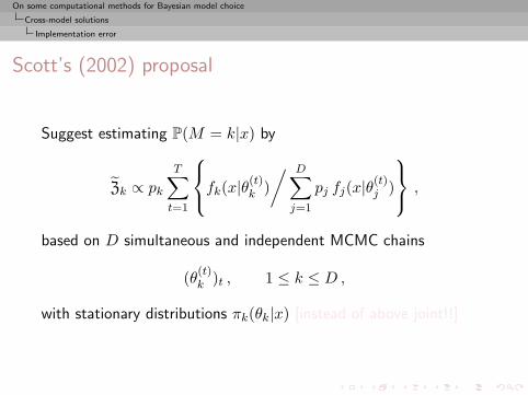
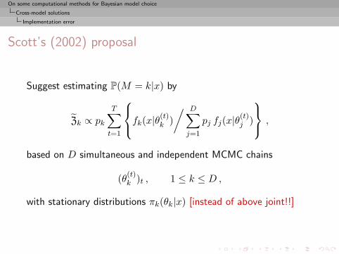
Scott’s (2002) proposal
Suggest estimating P(M = k|x) by
Zk ∝ pkT∑t=1
fk(x|θ(t)k )/ D∑
j=1
pj fj(x|θ(t)j )
,
based on D simultaneous and independent MCMC chains
(θ(t)k )t , 1 ≤ k ≤ D ,
with stationary distributions πk(θk|x) [instead of above joint!!]
On some computational methods for Bayesian model choice
Cross-model solutions
Implementation error
Congdon’s (2006) extension
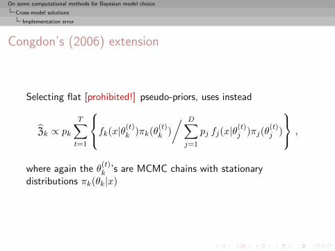
Selecting flat [prohibited!] pseudo-priors, uses instead
Zk ∝ pkT∑t=1
fk(x|θ(t)k )πk(θ
(t)k )/ D∑
j=1
pj fj(x|θ(t)j )πj(θ
(t)j )
,
where again the θ(t)k ’s are MCMC chains with stationary
distributions πk(θk|x)
On some computational methods for Bayesian model choice
Cross-model solutions
Implementation error
Examples
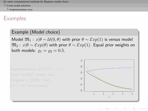
Example (Model choice)
Model M1 : x|θ ∼ U(0, θ) with prior θ ∼ Exp(1) is versus modelM2 : x|θ ∼ Exp(θ) with prior θ ∼ Exp(1). Equal prior weights onboth models: %1 = %2 = 0.5.
Approximations of P(M = 1|x):
Scott’s (2002) (blue), and
Congdon’s (2006) (red)
[N = 106 simulations].
1 2 3 4 5
0.0
0.2
0.4
0.6
0.8
1.0
y
On some computational methods for Bayesian model choice
Cross-model solutions
Implementation error
Examples
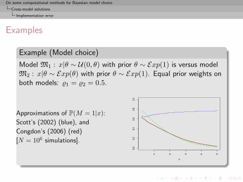
Example (Model choice)
Model M1 : x|θ ∼ U(0, θ) with prior θ ∼ Exp(1) is versus modelM2 : x|θ ∼ Exp(θ) with prior θ ∼ Exp(1). Equal prior weights onboth models: %1 = %2 = 0.5.
Approximations of P(M = 1|x):
Scott’s (2002) (blue), and
Congdon’s (2006) (red)
[N = 106 simulations].
1 2 3 4 5
0.0
0.2
0.4
0.6
0.8
1.0
y
On some computational methods for Bayesian model choice
Cross-model solutions
Implementation error
Examples (2)
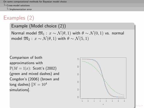
Example (Model choice (2))
Normal model M1 : x ∼ N (θ, 1) with θ ∼ N (0, 1) vs. normalmodel M2 : x ∼ N (θ, 1) with θ ∼ N (5, 1)
Comparison of both
approximations with
P(M = 1|x): Scott’s (2002)
(green and mixed dashes) and
Congdon’s (2006) (brown and
long dashes) [N = 104
simulations].
−1 0 1 2 3 4 5 6
0.0
0.2
0.4
0.6
0.8
1.0
y
On some computational methods for Bayesian model choice
Cross-model solutions
Implementation error
Examples (3)
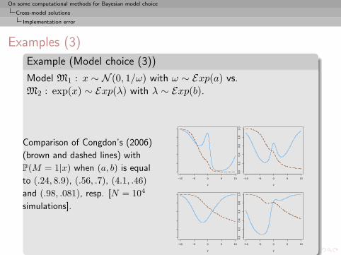
Example (Model choice (3))
Model M1 : x ∼ N (0, 1/ω) with ω ∼ Exp(a) vs.M2 : exp(x) ∼ Exp(λ) with λ ∼ Exp(b).
Comparison of Congdon’s (2006)
(brown and dashed lines) with
P(M = 1|x) when (a, b) is equal
to (.24, 8.9), (.56, .7), (4.1, .46)and (.98, .081), resp. [N = 104
simulations].
−10 −5 0 5 10
0.0
0.2
0.4
0.6
0.8
1.0
y
−10 −5 0 5 10
0.0
0.2
0.4
0.6
0.8
1.0
y
−10 −5 0 5 10
0.0
0.2
0.4
0.6
0.8
1.0
y
−10 −5 0 5 10
0.0
0.2
0.4
0.6
0.8
1.0
y

On some computational methods for Bayesian model choice
Nested sampling
Purpose
Nested sampling: Goal
Skilling’s (2007) technique using the one-dimensionalrepresentation:
Z = Eπ[L(θ)] =∫ 1
0ϕ(x) dx
withϕ−1(l) = P π(L(θ) > l).
Note; ϕ(·) is intractable in most cases.
On some computational methods for Bayesian model choice
Nested sampling
Implementation
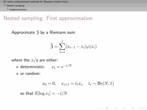
Nested sampling: First approximation
Approximate Z by a Riemann sum:
Z =j∑i=1
(xi−1 − xi)ϕ(xi)
where the xi’s are either:
deterministic: xi = e−i/N
or random:
x0 = 0, xi+1 = tixi, ti ∼ Be(N, 1)
so that E[log xi] = −i/N .
On some computational methods for Bayesian model choice
Nested sampling
Implementation
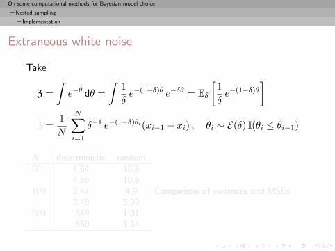
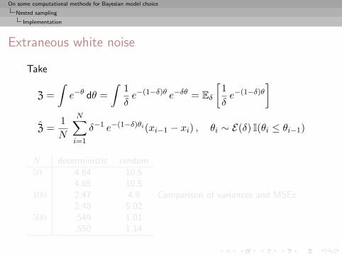
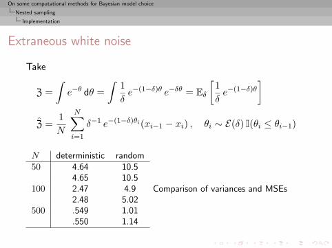
Extraneous white noise
Take
Z =∫e−θ dθ =
∫1δe−(1−δ)θ e−δθ = Eδ
[1δe−(1−δ)θ
]Z =
1N
N∑i=1
δ−1 e−(1−δ)θi(xi−1 − xi) , θi ∼ E(δ) I(θi ≤ θi−1)
N deterministic random50 4.64 10.5
4.65 10.5100 2.47 4.9
2.48 5.02500 .549 1.01
.550 1.14
Comparison of variances and MSEs
On some computational methods for Bayesian model choice
Nested sampling
Implementation
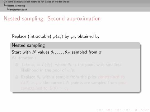
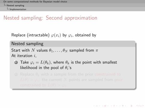
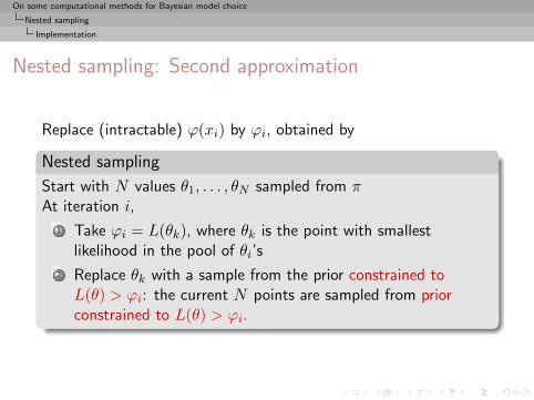
Nested sampling: Second approximation
Replace (intractable) ϕ(xi) by ϕi, obtained by
Nested sampling
Start with N values θ1, . . . , θN sampled from πAt iteration i,
1 Take ϕi = L(θk), where θk is the point with smallestlikelihood in the pool of θi’s
2 Replace θk with a sample from the prior constrained toL(θ) > ϕi: the current N points are sampled from priorconstrained to L(θ) > ϕi.
On some computational methods for Bayesian model choice
Nested sampling
Implementation
Nested sampling: Third approximation
Iterate the above steps until a given stopping iteration j isreached: e.g.,
observe very small changes in the approximation Z;
reach the maximal value of L(θ) when the likelihood isbounded and its maximum is known;
truncate the integral Z at level ε, i.e. replace∫ 1
0ϕ(x) dx with
∫ 1
εϕ(x) dx
On some computational methods for Bayesian model choice
Nested sampling
Error rates
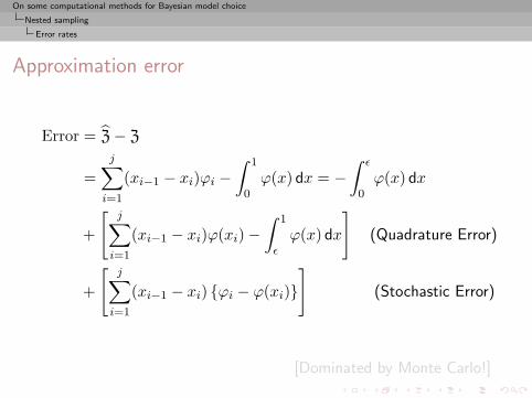
Approximation error
Error = Z− Z
=j∑i=1
(xi−1 − xi)ϕi −∫ 1
0ϕ(x) dx = −
∫ ε
0ϕ(x) dx (Truncation Error)
+
[j∑i=1
(xi−1 − xi)ϕ(xi)−∫ 1
εϕ(x) dx
](Quadrature Error)
+
[j∑i=1
(xi−1 − xi) {ϕi − ϕ(xi)}
](Stochastic Error)
[Dominated by Monte Carlo!]
On some computational methods for Bayesian model choice
Nested sampling
Error rates
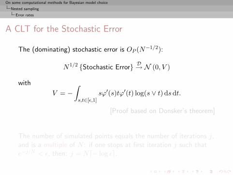
A CLT for the Stochastic Error
The (dominating) stochastic error is OP (N−1/2):
N1/2 {Stochastic Error} D→ N (0, V )
with
V = −∫s,t∈[ε,1]
sϕ′(s)tϕ′(t) log(s ∨ t) ds dt.
[Proof based on Donsker’s theorem]
The number of simulated points equals the number of iterations j,and is a multiple of N : if one stops at first iteration j such thate−j/N < ε, then: j = Nd− log εe.
On some computational methods for Bayesian model choice
Nested sampling
Error rates
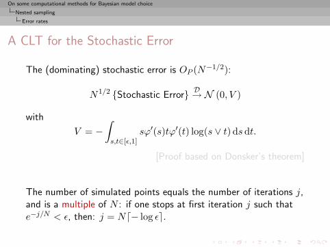
A CLT for the Stochastic Error
The (dominating) stochastic error is OP (N−1/2):
N1/2 {Stochastic Error} D→ N (0, V )
with
V = −∫s,t∈[ε,1]
sϕ′(s)tϕ′(t) log(s ∨ t) ds dt.
[Proof based on Donsker’s theorem]
The number of simulated points equals the number of iterations j,and is a multiple of N : if one stops at first iteration j such thate−j/N < ε, then: j = Nd− log εe.
On some computational methods for Bayesian model choice
Nested sampling
Impact of dimension
Curse of dimension
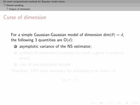
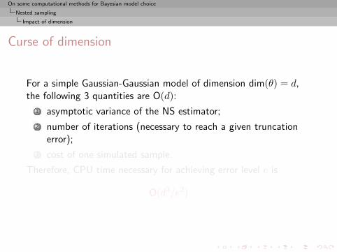
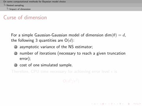
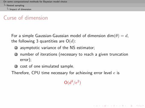
For a simple Gaussian-Gaussian model of dimension dim(θ) = d,the following 3 quantities are O(d):
1 asymptotic variance of the NS estimator;
2 number of iterations (necessary to reach a given truncationerror);
3 cost of one simulated sample.
Therefore, CPU time necessary for achieving error level e is
O(d3/e2)
On some computational methods for Bayesian model choice
Nested sampling
Impact of dimension
Curse of dimension
For a simple Gaussian-Gaussian model of dimension dim(θ) = d,the following 3 quantities are O(d):
1 asymptotic variance of the NS estimator;
2 number of iterations (necessary to reach a given truncationerror);
3 cost of one simulated sample.
Therefore, CPU time necessary for achieving error level e is
O(d3/e2)
On some computational methods for Bayesian model choice
Nested sampling
Constraints
Sampling from constr’d priors
Exact simulation from the constrained prior is intractable in mostcases!
Skilling (2007) proposes to use MCMC, but:
this introduces a bias (stopping rule).
if MCMC stationary distribution is unconst’d prior, more andmore difficult to sample points such that L(θ) > l as lincreases.
If implementable, then slice sampler can be devised at the samecost!
On some computational methods for Bayesian model choice
Nested sampling
Constraints
Illustration of MCMC bias
10 20 30 40 50 60 70 80 90100-50
-40
-30
-20
-10
0
10N=100, M=1
10 20 30 40 50 60 70 80 90100
-4
-2
0
2
4
N=100, M=3
10 20 30 40 50 60 70 80 90100
-4
-2
0
2
4
N=100, M=5
0 20 40 60 80 1000
10000
20000
30000
40000
50000
60000
70000
80000N=100, M=5
10 20 30 40 50 60 70 80 90100-10
-5
0
5
10N=500, M=1
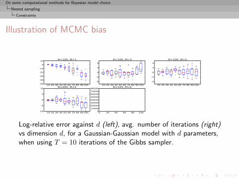
Log-relative error against d (left), avg. number of iterations (right)vs dimension d, for a Gaussian-Gaussian model with d parameters,when using T = 10 iterations of the Gibbs sampler.
On some computational methods for Bayesian model choice
Nested sampling
Importance variant
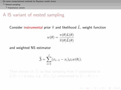
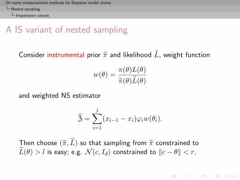
A IS variant of nested sampling
Consider instrumental prior π and likelihood L, weight function
w(θ) =π(θ)L(θ)
π(θ)L(θ)
and weighted NS estimator
Z =j∑i=1
(xi−1 − xi)ϕiw(θi).
Then choose (π, L) so that sampling from π constrained toL(θ) > l is easy; e.g. N (c, Id) constrained to ‖c− θ‖ < r.
On some computational methods for Bayesian model choice
Nested sampling
Importance variant
A IS variant of nested sampling
Consider instrumental prior π and likelihood L, weight function
w(θ) =π(θ)L(θ)
π(θ)L(θ)
and weighted NS estimator
Z =j∑i=1
(xi−1 − xi)ϕiw(θi).
Then choose (π, L) so that sampling from π constrained toL(θ) > l is easy; e.g. N (c, Id) constrained to ‖c− θ‖ < r.
On some computational methods for Bayesian model choice
Nested sampling
A mixture comparison
Benchmark: Target distribution
Posterior distribution on (µ, σ) associated with the mixture
pN (0, 1) + (1− p)N (µ, σ) ,
when p is known
On some computational methods for Bayesian model choice
Nested sampling
A mixture comparison
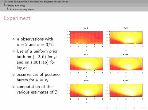
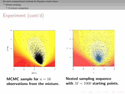
Experiment
n observations withµ = 2 and σ = 3/2,
Use of a uniform priorboth on (−2, 6) for µand on (.001, 16) forlog σ2.
occurrences of posteriorbursts for µ = xi
computation of thevarious estimates of Z
On some computational methods for Bayesian model choice
Nested sampling
A mixture comparison
Experiment (cont’d)
MCMC sample for n = 16observations from the mixture.
Nested sampling sequencewith M = 1000 starting points.
On some computational methods for Bayesian model choice
Nested sampling
A mixture comparison
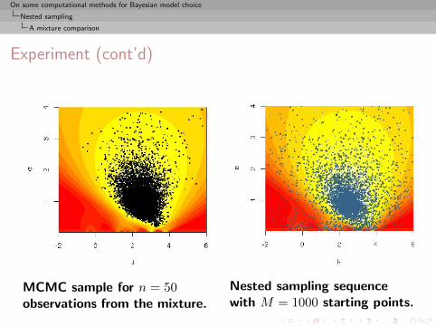
Experiment (cont’d)
MCMC sample for n = 50observations from the mixture.
Nested sampling sequencewith M = 1000 starting points.
On some computational methods for Bayesian model choice
Nested sampling
A mixture comparison
Comparison
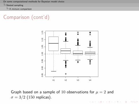
Monte Carlo and MCMC (=Gibbs) outputs based on T = 104
simulations and numerical integration based on a 850× 950 grid inthe (µ, σ) parameter space.Nested sampling approximation based on a starting sample ofM = 1000 points followed by at least 103 further simulations fromthe constr’d prior and a stopping rule at 95% of the observedmaximum likelihood.Constr’d prior simulation based on 50 values simulated by randomwalk accepting only steps leading to a lik’hood higher than thebound
On some computational methods for Bayesian model choice
Nested sampling
A mixture comparison
Comparison (cont’d)
●
●●
●
●●
●
●
●
●●
●
●
●
●
●
●
●
●
●
●
●●
●
●
●
●
●●
●
●
●
●
●
●
●
●
●●
●
●
●
●
●
●
●
●
●
●
●●
●●
●
●●
●
●
●
●
●
●
●
●●
●
●
●●
●
●
V1 V2 V3 V4
0.85
0.90
0.95
1.00
1.05
1.10
1.15
Graph based on a sample of 10 observations for µ = 2 andσ = 3/2 (150 replicas).

On some computational methods for Bayesian model choice
Nested sampling
A mixture comparison
Comparison (cont’d)
●
●
●
●
●
●●
●
●
V1 V2 V3 V4
0.90
0.95
1.00
1.05
1.10
Graph based on a sample of 50 observations for µ = 2 andσ = 3/2 (150 replicas).
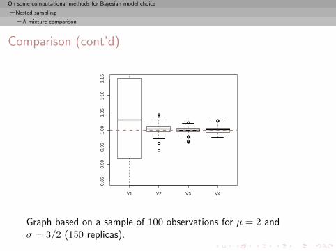
On some computational methods for Bayesian model choice
Nested sampling
A mixture comparison
Comparison (cont’d)
●
●
●●
●
●●●
●
●
●
●●
V1 V2 V3 V4
0.85
0.90
0.95
1.00
1.05
1.10
1.15
Graph based on a sample of 100 observations for µ = 2 andσ = 3/2 (150 replicas).
On some computational methods for Bayesian model choice
Nested sampling
A mixture comparison
Comparison (cont’d)
Nested sampling gets less reliable as sample size increasesMost reliable approach is mixture Z3 although harmonic solutionZ1 close to Chib’s solution [taken as golden standard]Monte Carlo method Z2 also producing poor approximations to Z
(Kernel φ used in Z2 is a t non-parametric kernel estimate withstandard bandwidth estimation.)
On some computational methods for Bayesian model choice
ABC model choice
ABC method
Approximate Bayesian Computation
Bayesian setting: target is π(θ)f(x|θ)When likelihood f(x|θ) not in closed form, likelihood-free rejectiontechnique:
ABC algorithm
For an observation y ∼ f(y|θ), under the prior π(θ), keep jointlysimulating
θ′ ∼ π(θ) , x ∼ f(x|θ′) ,
until the auxiliary variable x is equal to the observed value, x = y.
[Pritchard et al., 1999]
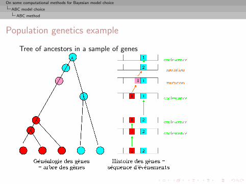
On some computational methods for Bayesian model choice
ABC model choice
ABC method
Population genetics example
Tree of ancestors in a sample of genes
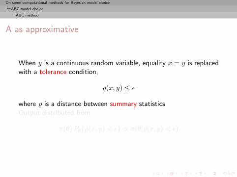
On some computational methods for Bayesian model choice
ABC model choice
ABC method
A as approximative
When y is a continuous random variable, equality x = y is replacedwith a tolerance condition,
%(x, y) ≤ ε
where % is a distance between summary statisticsOutput distributed from
π(θ)Pθ{%(x, y) < ε} ∝ π(θ|%(x, y) < ε)
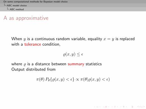

On some computational methods for Bayesian model choice
ABC model choice
ABC method
ABC improvements
Simulating from the prior is often poor in efficiencyEither modify the proposal distribution on θ to increase the densityof x’s within the vicinity of y...
[Marjoram et al, 2003; Bortot et al., 2007, Sisson et al., 2007]
...or by viewing the problem as a conditional density estimationand by developing techniques to allow for larger ε
[Beaumont et al., 2002]
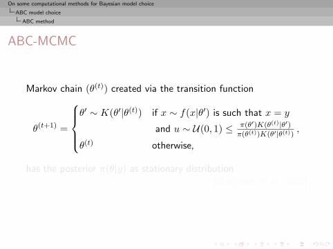
On some computational methods for Bayesian model choice
ABC model choice
ABC method
ABC-MCMC
Markov chain (θ(t)) created via the transition function
θ(t+1) =
θ′ ∼ K(θ′|θ(t)) if x ∼ f(x|θ′) is such that x = y
and u ∼ U(0, 1) ≤ π(θ′)K(θ(t)|θ′)π(θ(t))K(θ′|θ(t)) ,
θ(t) otherwise,
has the posterior π(θ|y) as stationary distribution[Marjoram et al, 2003]

On some computational methods for Bayesian model choice
ABC model choice
ABC method
ABC-PRC
Another sequential version producing a sequence of Markov
transition kernels Kt and of samples (θ(t)1 , . . . , θ
(t)N ) (1 ≤ t ≤ T )
ABC-PRC Algorithm
1 Pick a θ? is selected at random among the previous θ(t−1)i ’s
with probabilities ω(t−1)i (1 ≤ i ≤ N).
2 Generateθ
(t)i ∼ Kt(θ|θ?) , x ∼ f(x|θ(t)
i ) ,
3 Check that %(x, y) < ε, otherwise start again.
[Sisson et al., 2007]
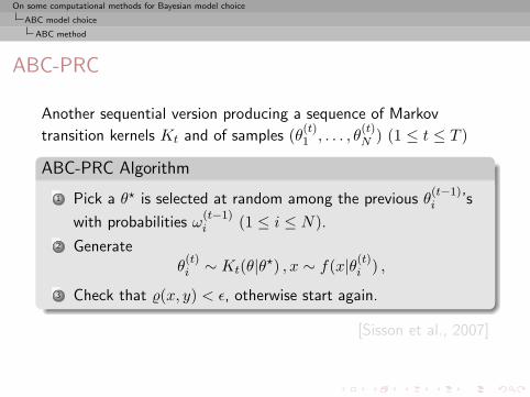
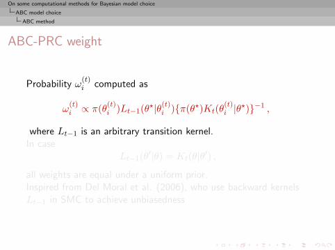
On some computational methods for Bayesian model choice
ABC model choice
ABC method
ABC-PRC weight
Probability ω(t)i computed as
ω(t)i ∝ π(θ(t)
i )Lt−1(θ?|θ(t)i ){π(θ?)Kt(θ
(t)i |θ
?)}−1 ,
where Lt−1 is an arbitrary transition kernel.In case
Lt−1(θ′|θ) = Kt(θ|θ′) ,
all weights are equal under a uniform prior.Inspired from Del Moral et al. (2006), who use backward kernelsLt−1 in SMC to achieve unbiasedness
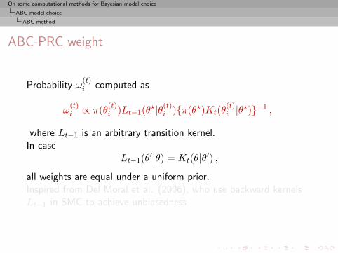

On some computational methods for Bayesian model choice
ABC model choice
ABC method
ABC-PRC bias
Lack of unbiasedness of the methodJoint density of the accepted pair (θ(t−1), θ(t)) proportional to
π(θ(t−1)|y)Kt(θ(t)|θ(t−1))f(y|θ(t)) ,
For an arbitrary function h(θ), E[ωth(θ(t))] proportional to
ZZh(θ
(t))π(θ(t))Lt−1(θ(t−1)|θ(t))π(θ(t−1))Kt(θ(t)|θ(t−1))
π(θ(t−1)|y)Kt(θ(t)|θ(t−1)
)f(y|θ(t))dθ(t−1)dθ(t)
∝ZZ
h(θ(t)
)π(θ(t))Lt−1(θ(t−1)|θ(t))π(θ(t−1))Kt(θ(t)|θ(t−1))
π(θ(t−1)
)f(y|θ(t−1))
×Kt(θ(t)|θ(t−1))f(y|θ(t))dθ(t−1)dθ(t)
∝Zh(θ
(t))π(θ
(t)|y)Z
Lt−1(θ(t−1)|θ(t))f(y|θ(t−1)
)dθ(t−1)ff
dθ(t) .
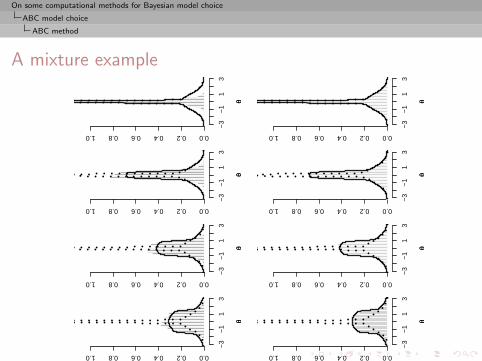
On some computational methods for Bayesian model choice
ABC model choice
ABC method
A mixture example
θθ
−3
−1
13
0.00.20.40.60.81.0
θθ
−3
−1
13
0.00.20.40.60.81.0
θθ
−3
−1
13
0.00.20.40.60.81.0
θθ
−3
−1
13
0.00.20.40.60.81.0
θθ
−3
−1
13
0.00.20.40.60.81.0
θθ
−3
−1
13
0.00.20.40.60.81.0
θθ
−3
−1
13
0.00.20.40.60.81.0
θθ
−3
−1
13
0.00.20.40.60.81.0
θθ
−3
−1
13
0.00.20.40.60.81.0
θθ
−3
−1
13
0.00.20.40.60.81.0
Comparison of τ = 0.15 and τ = 1/0.15 in Kt
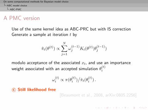
On some computational methods for Bayesian model choice
ABC model choice
ABC-PMC
A PMC version
Use of the same kernel idea as ABC-PRC but with IS correctionGenerate a sample at iteration t by
πt(θ(t)) ∝N∑j=1
ω(t−1)j Kt(θ(t)|θ(t−1)
j )
modulo acceptance of the associated xt, and use an importance
weight associated with an accepted simulation θ(t)i
ω(t)i ∝ π(θ(t)
i )/πt(θ
(t)i ) .
c© Still likelihood free[Beaumont et al., 2008, arXiv:0805.2256]
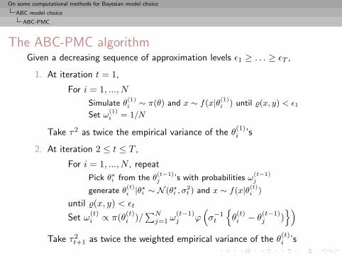
On some computational methods for Bayesian model choice
ABC model choice
ABC-PMC
The ABC-PMC algorithmGiven a decreasing sequence of approximation levels ε1 ≥ . . . ≥ εT ,
1. At iteration t = 1,
For i = 1, ..., NSimulate θ
(1)i ∼ π(θ) and x ∼ f(x|θ(1)i ) until %(x, y) < ε1
Set ω(1)i = 1/N
Take τ2 as twice the empirical variance of the θ(1)i ’s
2. At iteration 2 ≤ t ≤ T ,
For i = 1, ..., N , repeat
Pick θ?i from the θ(t−1)j ’s with probabilities ω
(t−1)j
generate θ(t)i |θ
?i ∼ N (θ?i , σ
2t ) and x ∼ f(x|θ(t)i )
until %(x, y) < εt
Set ω(t)i ∝ π(θ(t)i )/
∑Nj=1 ω
(t−1)j ϕ
(σ−1t
{θ(t)i − θ
(t−1)j )
})Take τ2
t+1 as twice the weighted empirical variance of the θ(t)i ’s
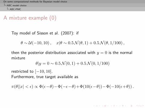
On some computational methods for Bayesian model choice
ABC model choice
ABC-PMC
A mixture example (0)
Toy model of Sisson et al. (2007): if
θ ∼ U(−10, 10) , x|θ ∼ 0.5N (θ, 1) + 0.5N (θ, 1/100) ,
then the posterior distribution associated with y = 0 is the normalmixture
θ|y = 0 ∼ 0.5N (0, 1) + 0.5N (0, 1/100)
restricted to [−10, 10].Furthermore, true target available as
π(θ||x| < ε) ∝ Φ(ε−θ)−Φ(−ε−θ)+Φ(10(ε−θ))−Φ(−10(ε+θ)) .
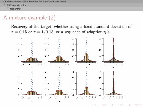
On some computational methods for Bayesian model choice
ABC model choice
ABC-PMC
A mixture example (2)
Recovery of the target, whether using a fixed standard deviation ofτ = 0.15 or τ = 1/0.15, or a sequence of adaptive τt’s.

On some computational methods for Bayesian model choice
ABC model choice
ABC for model choice in GRFs
Gibbs random fields
Gibbs distribution
The rv y = (y1, . . . , yn) is a Gibbs random field associated withthe graph G if
f(y) =1Z
exp
{−∑c∈C
Vc(yc)
},
where Z is the normalising constant, C is the set of cliques of G
and Vc is any function also called potentialU(y) =
∑c∈C Vc(yc) is the energy function
c© Z is usually unavailable in closed form
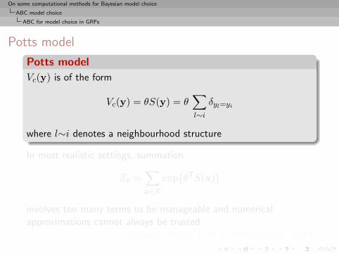
On some computational methods for Bayesian model choice
ABC model choice
ABC for model choice in GRFs
Potts model
Potts model
Vc(y) is of the form
Vc(y) = θS(y) = θ∑l∼i
δyl=yi
where l∼i denotes a neighbourhood structure
In most realistic settings, summation
Zθ =∑x∈X
exp{θTS(x)}
involves too many terms to be manageable and numericalapproximations cannot always be trusted
[Cucala, Marin, CPR & Titterington, 2009]
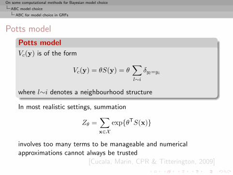
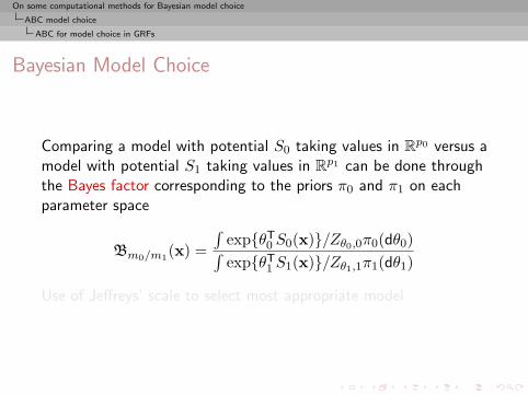
On some computational methods for Bayesian model choice
ABC model choice
ABC for model choice in GRFs
Bayesian Model Choice
Comparing a model with potential S0 taking values in Rp0 versus amodel with potential S1 taking values in Rp1 can be done throughthe Bayes factor corresponding to the priors π0 and π1 on eachparameter space
Bm0/m1(x) =
∫exp{θT
0 S0(x)}/Zθ0,0π0(dθ0)∫exp{θT
1 S1(x)}/Zθ1,1π1(dθ1)
Use of Jeffreys’ scale to select most appropriate model
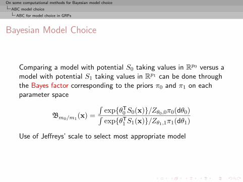
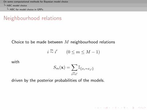
On some computational methods for Bayesian model choice
ABC model choice
ABC for model choice in GRFs
Neighbourhood relations
Choice to be made between M neighbourhood relations
im∼ i′ (0 ≤ m ≤M − 1)
withSm(x) =
∑im∼i′
I{xi=xi′}
driven by the posterior probabilities of the models.
On some computational methods for Bayesian model choice
ABC model choice
ABC for model choice in GRFs
Model index
Formalisation via a model index M that appears as a newparameter with prior distribution π(M = m) andπ(θ|M = m) = πm(θm)Computational target:
P(M = m|x) ∝∫
Θm
fm(x|θm)πm(θm) dθm π(M = m) ,
On some computational methods for Bayesian model choice
ABC model choice
ABC for model choice in GRFs
Sufficient statisticsBy definition, if S(x) sufficient statistic for the joint parameters(M, θ0, . . . , θM−1),
P(M = m|x) = P(M = m|S(x)) .
For each model m, own sufficient statistic Sm(·) andS(·) = (S0(·), . . . , SM−1(·)) also sufficient.For Gibbs random fields,
x|M = m ∼ fm(x|θm) = f1m(x|S(x))f2
m(S(x)|θm)
=1
n(S(x))f2m(S(x)|θm)
wheren(S(x)) = ] {x ∈ X : S(x) = S(x)}
c© S(x) is therefore also sufficient for the joint parameters[Specific to Gibbs random fields!]
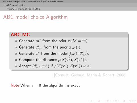
On some computational methods for Bayesian model choice
ABC model choice
ABC for model choice in GRFs
ABC model choice Algorithm
ABC-MC
Generate m∗ from the prior π(M = m).
Generate θ∗m∗ from the prior πm∗(·).
Generate x∗ from the model fm∗(·|θ∗m∗).
Compute the distance ρ(S(x0), S(x∗)).
Accept (θ∗m∗ ,m∗) if ρ(S(x0), S(x∗)) < ε.
[Cornuet, Grelaud, Marin & Robert, 2008]
Note When ε = 0 the algorithm is exact
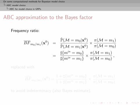
On some computational methods for Bayesian model choice
ABC model choice
ABC for model choice in GRFs
ABC approximation to the Bayes factor
Frequency ratio:
BFm0/m1(x0) =
P(M = m0|x0)P(M = m1|x0)
× π(M = m1)π(M = m0)
=]{mi∗ = m0}]{mi∗ = m1}
× π(M = m1)π(M = m0)
,
replaced with
BFm0/m1(x0) =
1 + ]{mi∗ = m0}1 + ]{mi∗ = m1}
× π(M = m1)π(M = m0)
to avoid indeterminacy (also Bayes estimate).
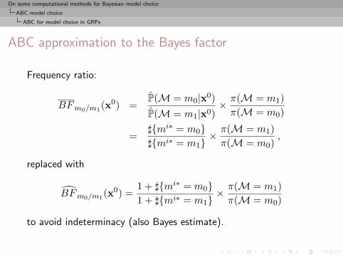
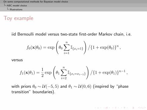
On some computational methods for Bayesian model choice
ABC model choice
Illustrations
Toy example
iid Bernoulli model versus two-state first-order Markov chain, i.e.
f0(x|θ0) = exp
(θ0
n∑i=1
I{xi=1}
)/{1 + exp(θ0)}n ,
versus
f1(x|θ1) =12
exp
(θ1
n∑i=2
I{xi=xi−1}
)/{1 + exp(θ1)}n−1 ,
with priors θ0 ∼ U(−5, 5) and θ1 ∼ U(0, 6) (inspired by “phasetransition” boundaries).
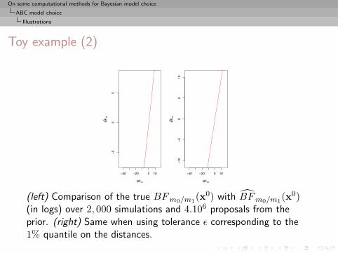
On some computational methods for Bayesian model choice
ABC model choice
Illustrations
Toy example (2)
−40 −20 0 10
−50
5
BF01
BF01
−40 −20 0 10−10
−50
510
BF01
BF01
(left) Comparison of the true BFm0/m1(x0) with BFm0/m1
(x0)(in logs) over 2, 000 simulations and 4.106 proposals from theprior. (right) Same when using tolerance ε corresponding to the1% quantile on the distances.
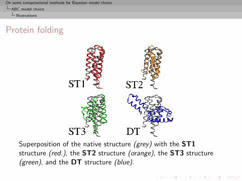
On some computational methods for Bayesian model choice
ABC model choice
Illustrations
Protein folding
Superposition of the native structure (grey) with the ST1structure (red.), the ST2 structure (orange), the ST3 structure(green), and the DT structure (blue).
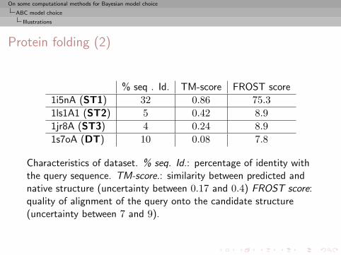
On some computational methods for Bayesian model choice
ABC model choice
Illustrations
Protein folding (2)
% seq . Id. TM-score FROST score
1i5nA (ST1) 32 0.86 75.31ls1A1 (ST2) 5 0.42 8.91jr8A (ST3) 4 0.24 8.91s7oA (DT) 10 0.08 7.8
Characteristics of dataset. % seq. Id.: percentage of identity withthe query sequence. TM-score.: similarity between predicted andnative structure (uncertainty between 0.17 and 0.4) FROST score:quality of alignment of the query onto the candidate structure(uncertainty between 7 and 9).
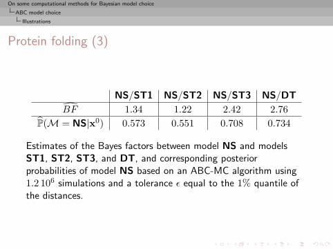
On some computational methods for Bayesian model choice
ABC model choice
Illustrations
Protein folding (3)
NS/ST1 NS/ST2 NS/ST3 NS/DT
BF 1.34 1.22 2.42 2.76P(M = NS|x0) 0.573 0.551 0.708 0.734
Estimates of the Bayes factors between model NS and modelsST1, ST2, ST3, and DT, and corresponding posteriorprobabilities of model NS based on an ABC-MC algorithm using1.2 106 simulations and a tolerance ε equal to the 1% quantile ofthe distances.


