Halonen 2nd ed
48
6 GSM/AMR and SAIC Voice Performance Juan Melero, Ruben Cruz, Timo Halonen, Jari Hulkkonen, Jeroen Wigard, Angel-Luis Rivada, Martti Moisio, Tommy Bysted, Mark Austin, Laurie Bigler, Ayman Mostafa and Rich Kobylinski and Benoist Sebireto Despite the expected growth of data services, conventional speech will be the dominant revenue generation service for many years. As voice traffic continues growing, many net- works are facing capacity challenges, which may be addressed with the right technology deployment. This chapter presents the global system for mobile communications (GSM) voice performance, highlighting the spectral efficiency enhancements achievable with dif- ferent functionality. Section 6.1 introduces the performance improvements associated with basic baseline GSM speech performance functionality (as defined in Chapter 5), which includes frequency hopping (FH), power control (PC) and discontinuous transmission (DTX). In Section 6.2, frequency reuse partitioning methods are presented. Section 6.3 presents trunking gain GSM functionality such as traffic reason handover (TRHO) or Directed retry (DR). Half rate is introduced in Section 6.4. Rel’98 adaptive multi-rate (AMR) is thoroughly analysed in Section 6.5 and Source Adaptation is presented in Section 6.6. Section 6.7 introduces Rel’5 EDGE AMR enhancements and finally, SAIC functionality performance gains are presented in Section 6.8. The performance results described in this chapter include comprehensive simulations and field trials with real networks around the world. 6.1 Basic GSM Performance This section will describe the network level performance enhancements associated with the basic set of standard GSM functionality defined in the previous chapter: FH, PC and DTX. Section 5.5 in Chapter 5 introduced the GSM baseline network performance based on the deployment of this basic set. GSM, GPRS and EDGE Performance 2 nd Ed. Edited by T. Halonen, J. Romero and J. Melero 2003 John Wiley & Sons, Ltd ISBN: 0-470-86694-2
-
Upload
emerson-eduardo-rodrigues-pmp -
Category
Documents
-
view
267 -
download
0
Transcript of Halonen 2nd ed

6
GSM/AMR and SAIC VoicePerformanceJuan Melero, Ruben Cruz, Timo Halonen, Jari Hulkkonen,Jeroen Wigard, Angel-Luis Rivada, Martti Moisio, Tommy Bysted,Mark Austin, Laurie Bigler, Ayman Mostafa and Rich Kobylinski andBenoist Sebireto
Despite the expected growth of data services, conventional speech will be the dominantrevenue generation service for many years. As voice traffic continues growing, many net-works are facing capacity challenges, which may be addressed with the right technologydeployment. This chapter presents the global system for mobile communications (GSM)voice performance, highlighting the spectral efficiency enhancements achievable with dif-ferent functionality. Section 6.1 introduces the performance improvements associated withbasic baseline GSM speech performance functionality (as defined in Chapter 5), whichincludes frequency hopping (FH), power control (PC) and discontinuous transmission(DTX). In Section 6.2, frequency reuse partitioning methods are presented. Section 6.3presents trunking gain GSM functionality such as traffic reason handover (TRHO) orDirected retry (DR). Half rate is introduced in Section 6.4. Rel’98 adaptive multi-rate(AMR) is thoroughly analysed in Section 6.5 and Source Adaptation is presented inSection 6.6. Section 6.7 introduces Rel’5 EDGE AMR enhancements and finally, SAICfunctionality performance gains are presented in Section 6.8. The performance resultsdescribed in this chapter include comprehensive simulations and field trials with realnetworks around the world.
6.1 Basic GSM PerformanceThis section will describe the network level performance enhancements associated withthe basic set of standard GSM functionality defined in the previous chapter: FH, PC andDTX. Section 5.5 in Chapter 5 introduced the GSM baseline network performance basedon the deployment of this basic set.
GSM, GPRS and EDGE Performance 2nd Ed. Edited by T. Halonen, J. Romero and J. Melero 2003 John Wiley & Sons, Ltd ISBN: 0-470-86694-2
188 GSM, GPRS and EDGE Performance
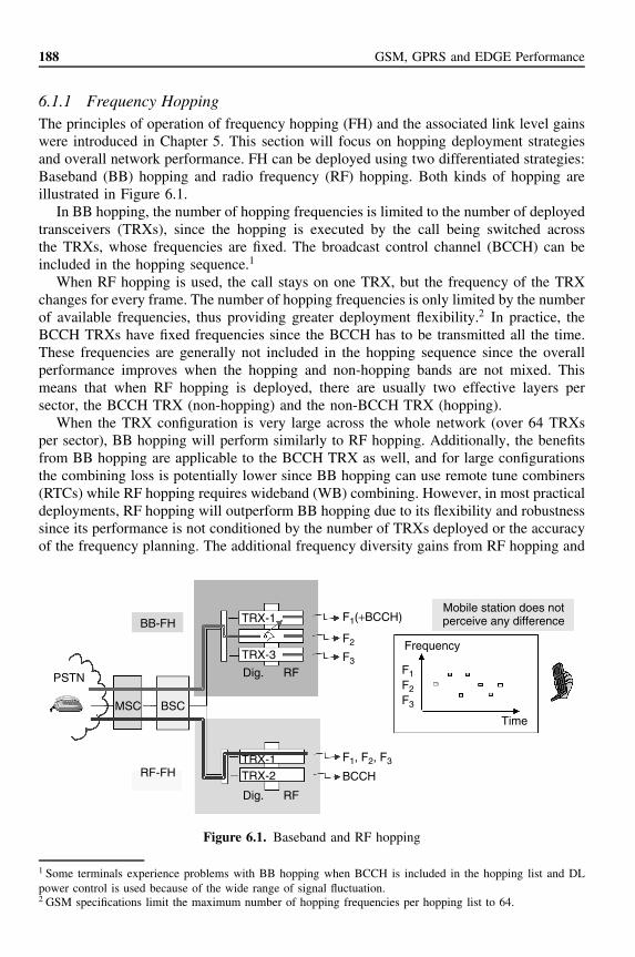
6.1.1 Frequency HoppingThe principles of operation of frequency hopping (FH) and the associated link level gainswere introduced in Chapter 5. This section will focus on hopping deployment strategiesand overall network performance. FH can be deployed using two differentiated strategies:Baseband (BB) hopping and radio frequency (RF) hopping. Both kinds of hopping areillustrated in Figure 6.1.
In BB hopping, the number of hopping frequencies is limited to the number of deployedtransceivers (TRXs), since the hopping is executed by the call being switched acrossthe TRXs, whose frequencies are fixed. The broadcast control channel (BCCH) can beincluded in the hopping sequence.1
When RF hopping is used, the call stays on one TRX, but the frequency of the TRXchanges for every frame. The number of hopping frequencies is only limited by the numberof available frequencies, thus providing greater deployment flexibility.2 In practice, theBCCH TRXs have fixed frequencies since the BCCH has to be transmitted all the time.These frequencies are generally not included in the hopping sequence since the overallperformance improves when the hopping and non-hopping bands are not mixed. Thismeans that when RF hopping is deployed, there are usually two effective layers persector, the BCCH TRX (non-hopping) and the non-BCCH TRX (hopping).
When the TRX configuration is very large across the whole network (over 64 TRXsper sector), BB hopping will perform similarly to RF hopping. Additionally, the benefitsfrom BB hopping are applicable to the BCCH TRX as well, and for large configurationsthe combining loss is potentially lower since BB hopping can use remote tune combiners(RTCs) while RF hopping requires wideband (WB) combining. However, in most practicaldeployments, RF hopping will outperform BB hopping due to its flexibility and robustnesssince its performance is not conditioned by the number of TRXs deployed or the accuracyof the frequency planning. The additional frequency diversity gains from RF hopping and
MSC BSC
BB-FH
RF-FH
PSTN Dig. RF
F1(+BCCH)
F1, F2, F3
BCCH
F2
F3F1
Frequency
Time
Mobile station does notperceive any difference
F2F3
TRX-1
TRX-3
Dig. RF
TRX-1
TRX-2
Figure 6.1. Baseband and RF hopping
1 Some terminals experience problems with BB hopping when BCCH is included in the hopping list and DLpower control is used because of the wide range of signal fluctuation.2 GSM specifications limit the maximum number of hopping frequencies per hopping list to 64.

GSM/AMR and SAIC Voice Performance 189
00.0
0.5
1.0
1.5
2.0
2.5
3.0
3.5
4.0
1 2 3
EFL (%)
DC
R (
%)
4 5 6
RF hoppingBB hopping
82%
00.00.51.01.52.02.53.03.5
5.04.54.0
1 2 3
EFL (%)
% F
ER
> 8
%
4 5 6
RF hoppingBB hopping
80%
Figure 6.2. Network 1 RF hopping versus BB hopping DCR and FER-trialled performance
the use of cross polarisation antennas and air combining will compensate for the potentialadditional combining losses. All the studies throughout this book have considered RFhopping deployments, although the performance of BB hopping would be equivalentunder the previously stated conditions.
Figure 6.2 displays the performance of the RF and BB hopping layers for Network 1in terms of dropped call rate (DCR) and frame erasure rate (FER). Since the averagenumber of TRXs per sector was 2.5, BB hopping gains were, in this case, not comparableto those of RF hopping.
With a hopping list of n frequencies, 64 × n different hopping sequences can be built.These are mainly defined by two parameters, as was explained in Chapter 5. Firstly, themobile allocation index offset (MAIO), which may take as many values as the numberof frequencies in the hopping list. Secondly, the hopping sequence number (HSN), whichmay take up to 64 different values. Two channels bearing the same HSN but differentMAIOs never use the same frequency on the same burst, while two channels usingdifferent HSNs only interfere with each other (1/n)th of the time.
One of the main hopping deployment criteria is the frequency reuse selection. Thedifferent frequency reuses are characterised with a reuse factor. The reuse factor indicatesthe sector cluster size in which each frequency is used only once. The reuse factor istypically denoted as x/y, where x is the site reuse factor and y the sector reuse factor.This means that a hopping reuse factor of 3/9, corresponds to a cellular network withnine different hopping lists which are used every three sites. FH started to be used in themid-1990s. Initially, conservative reuses, such as 3/9, were used. However, 3/9 minimumeffective reuse was limited to nine. Later on, 1/3 proved to be feasible and finally 1/1was considered by many experts as the optimum RF hopping frequency reuse. Figure 6.3illustrates the hopping standard reuses of 3/9, 1/3 and 1/1.
As the frequency reuse gets tighter, the interference distribution worsens, but, on theother hand, the associated FH gains increase. Figures 6.4 and 6.5 display the performanceof hopping reuses 1/1 and 3/9. The results are based on simulations using Network 1 prop-agation environment and traffic distribution. Reuse 3/9 shows better carrier/interference(C/I) distribution and therefore bit error rate (BER) performance. However, reuse 1/1has a better overall frame error rate (FER) performance due to the higher frequency andinterference diversity gains. As a conclusion, the most efficient hopping reuse will bedependent on the generated C/I distribution and the associated link level gains.

190 GSM, GPRS and EDGE Performance
Figure 6.3. Hopping standard reuses: 3/9, 1/3 and 1/1
101
10
100
1412 16 20 2418 22
CIR (dB)
Cum
mul
ativ
e pe
rcen
tage
(%
)
26 28 30
Reuse 1–1
Reuse 3–9
Better C/Idistribution
06065707580859095
100
10 20 30
BER (%)
Sam
ples
(%
)
40 50 60
Reuse 1–1
Reuse 3–9
Better BERperformance
Figure 6.4. C/I and BER Network 1 simulation performance
070
75
80
85
90
95
100
5 10 15
FER (%)
Cum
mul
ativ
e pe
rcen
tage
(%
)
20
Reuse 1–1
Reuse 3–9
Better FER
performance
Figure 6.5. FER Network 1 simulation performance

GSM/AMR and SAIC Voice Performance 191
Reuse 1/3 has proven to have equivalent or even slightly higher performance in deploy-ment scenarios with regular site distribution and antenna orientation. However, mostpractical networks are quite irregular both in terms of site distribution and antenna ori-entation. Reuse 1/1 has the advantage of better adaptability to any network topology andprovides higher hopping gains, especially in the case of limited number of available hop-ping frequencies. Finally, the MAIO management functionality can be used in the 1/1deployment to ensure that there is no interference between sectors of the same site.
The MAIO management functionality provides the ability to minimise the interferenceby controlling the MAIOs utilised by different TRXs within a synchronised site containingmultiple sectors. There are as many possible MAIOs as number of frequencies in thehopping list. Therefore, the number of TRXs that can be controlled within a site withoutrepetition of any MAIO value is limited by the number of hopping frequencies. Asthe effective reuses decrease, adjacent and co-channel interference (CCI) will begin tobe unavoidable within the sites. When this intra-site inter-sector interference is present,the use of different antenna beamwidth will impact the final performance. Appendix Aanalyses the MAIO management limitations, the best planning strategies and the impactof different antenna beamwidths.
Figure 6.6 displays the trial performance of RF hopping 1/3 and 1/1 when deployed inNetwork 2. In this typical network topology, both reuses had an equivalent performance.
The logic behind 1/1 being the best performing hopping reuse relies on the higherhopping gains for the higher number of frequencies. As presented in Chapter 5, most ofthe hopping gains are achieved with a certain number of hopping frequencies and furthergains associated with additional frequencies are not so high. On the other hand, reuse1/1 has the worst possible interference distribution. In order to get most hopping gains,to improve the interference distribution and to keep the high flexibility and adaptabilityassociated to 1/1 reuse, the innovative advanced reuse schemes (n/n) were devised. The
00
0.5
1
1.5
2
2.5
3
3.5
4
2 4 8
Effective frequency load (%)
Dro
p ca
ll ra
te
106
RF hop 1/3RF hop 1/1
Figure 6.6. Network 2 RF hopping 1/3 and 1/1 trialled performance

192 GSM, GPRS and EDGE Performance
idea is to introduce a site reuse in the system but keep the 1/1 scheme within each site.The end result is an improved C/I distribution while maintaining most of the link levelgains. Reuse 1/1 would belong to this category with a site reuse of 1. Figure 6.7 illustratessome examples of advanced reuse schemes.
The optimum FH advanced reuse scheme will be dependent on the number of availablefrequencies. For example, if 18 hopping frequencies are available, and assuming that 6frequencies provide most of the hopping gains, the optimum scheme would be 3/3. On theother hand, the MAIO management limitations presented in Appendix A are determinedby the number of hopping frequencies within the site and as n (reuse factor) increases theefficiency of MAIO management will decrease. Therefore, the optimum advanced reusescheme will be determined by both the total number of available hopping frequencies andthe existing TRX configuration.
Figure 6.8 shows the performance achieved by 1/1 and 2/2 reuses both in terms ofDCR and FER in Network 1 trials. The measured capacity increase ranged between 14and 18%. In this scenario, with 23 hopping frequencies available, reuse 3/3 is expectedto outperform both 1/1 and 2/2.
As a conclusion, the best performing hopping schemes are the RF hopping advancedreuse schemes. Additionally, these schemes do not require frequency planning or optimisa-tion in order to deliver their maximum associated performance. Other hopping deploymentstrategies can yield equivalent results, but have intensive planning and optimisation
Figure 6.7. Advanced reuse schemes. 1/1, 2/2 and 3/3
00.00.51.01.52.02.53.03.54.0
1 2 3
EFL (%)
DC
R (
%)
4 5 6
RF hopping 1/1 (non-BCCH)RF hopping 2/2 (non-BCCH)
00
1
2
3
4
5
6
7
1 2 3
EFL (%)
% F
ER
> 8
%
4 5 6
RF hopping 1/1 (non-BCCH)RF hopping 2/2 (non-BCCH)
18% 14%
Figure 6.8. Network 1 RF hopping 1/1 versus 2/2-trialled DCR and FER performance

GSM/AMR and SAIC Voice Performance 193
requirements in order to achieve their expected performance and are not so flexible inorder to be upgraded or re-planned. Examples of these other strategies could be BBhopping with large TRX configurations or heuristic planning,3 which require complexplanning tools and are very hard to optimise. These deployment strategies can make useof the automated planning functionality described in Chapter 13 in order to achieve highperformance without intensive planning and optimisation effort.
6.1.2 Power Control
Power control (PC) is an optional feature in GSM that reduces the interference in thesystem by reducing both the base station and mobile station transmitted power. Addition-ally, it contributes to extend the terminal’s battery life. The PC algorithm is described inmore detail in Chapter 5. PC can be efficiently combined with FH.
The control rate of PC is 0.48 s (once per slow associated control channel (SACCH)multiframe). For relatively slow moving mobiles, the interference reduction gain from PCcan be substantial, whereas for fast moving mobiles it may not be possible to efficientlytrack the signal variation. Hence, conservative power settings must be used, which limitsthe interference reduction gain. The average PC gain in carrier interference (C/I), measuredby network simulations including FH and for a mobile speed of 50 km/h, has been foundto be approximately 1.5 to 2.5 dB at a 10% outage level [1].
Figure 6.9 displays the impact of downlink power control (DL PC) in the distributionof received signal level. The 10-dB offset shows the efficiency of DL PC. Much higherdynamic ranges (range of power reduction) do not provide additional gains and, in somecases, can cause some problems since the DL PC speed may not be fast enough insome cases to follow the signal fading variations.
−100 to −900
20
40
60
80
100
−90 to −80 −80 to −70 −70 to −60 −60 to −50
Rx level (dBm)
%
−50 to 0
Figure 6.9. Network 1 DL PC trialled received signal level offset
3 Irregular hopping lists in order to optimise the C/I distribution.
194 GSM, GPRS and EDGE Performance
00
1
2
3
4
5
6
7
1 2 3
EFL (%)
% F
ER
> 8
%
4 5 6
RF hopping (non-BCCH)RF hopping + DL PC (non-BCCH)
47%
00.0
0.5
1.0
1.5
2.0
2.5
3.0
3.5
4.0
1 2 3
EFL (%)
DC
R (
%)
4 5 76
RF hopping (non-BCCH)RF hopping + DL PC (non-BCCH)
54.5%
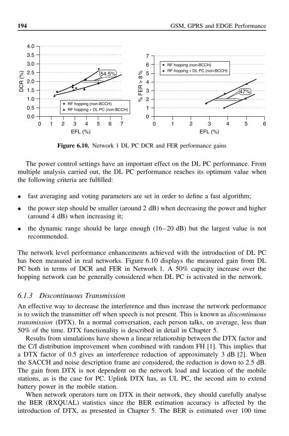
Figure 6.10. Network 1 DL PC DCR and FER performance gains
The power control settings have an important effect on the DL PC performance. Frommultiple analysis carried out, the DL PC performance reaches its optimum value whenthe following criteria are fulfilled:
• fast averaging and voting parameters are set in order to define a fast algorithm;
• the power step should be smaller (around 2 dB) when decreasing the power and higher(around 4 dB) when increasing it;
• the dynamic range should be large enough (16–20 dB) but the largest value is notrecommended.
The network level performance enhancements achieved with the introduction of DL PChas been measured in real networks. Figure 6.10 displays the measured gain from DLPC both in terms of DCR and FER in Network 1. A 50% capacity increase over thehopping network can be generally considered when DL PC is activated in the network.
6.1.3 Discontinuous Transmission
An effective way to decrease the interference and thus increase the network performanceis to switch the transmitter off when speech is not present. This is known as discontinuoustransmission (DTX). In a normal conversation, each person talks, on average, less than50% of the time. DTX functionality is described in detail in Chapter 5.
Results from simulations have shown a linear relationship between the DTX factor andthe C/I distribution improvement when combined with random FH [1]. This implies thata DTX factor of 0.5 gives an interference reduction of approximately 3 dB [2]. Whenthe SACCH and noise description frame are considered, the reduction is down to 2.5 dB.The gain from DTX is not dependent on the network load and location of the mobilestations, as is the case for PC. Uplink DTX has, as UL PC, the second aim to extendbattery power in the mobile station.
When network operators turn on DTX in their network, they should carefully analysethe BER (RXQUAL) statistics since the BER estimation accuracy is affected by theintroduction of DTX, as presented in Chapter 5. The BER is estimated over 100 time

GSM/AMR and SAIC Voice Performance 195
0RXQUAL RXQUAL
1 2 3 4 5 760.002.004.006.008.0010.0012.0014.0016.0018.0020.00
0.002.004.006.008.0010.0012.0014.0016.0018.0020.00
20.00
30.00
40.00
50.00
60.00
70.00
80.00
Per
cent
of o
ccur
ance
RX
QU
AL
0 (%
)
20.00
30.00
40.00
50.00
60.00
70.00
80.00
Per
cent
of o
ccur
ance
RX
QU
AL
0 (%
)
Per
cent
of o
ccur
ance
RX
QU
AL
1-7
(%)
Per
cent
of o
ccur
ance
RX
QU
AL
1-7
(%)
0 1 2 3 4 5 6 7
1/3, FULL1/3, SUB3/9, FULL3/9, SUB
(a) (b)
Cell 1, FULLCell 1, SUBCell 2, FULLCell 2, SUB
Figure 6.11. Simulations (a) and Network 8 (b) RXQUAL-FULL and RXQUAL-SUBdistribution
division multiple access (TDMA) bursts in the non-DTX mode and over 12 TDMA burstsin the DTX mode. The first is called RXQUAL-FULL and the second RXQUAL-SUB.
Network simulations showed that the higher variance causes the RXQUAL-SUB valuesto be more spread when compared with the RXQUAL-FULL values. While the networkactually gets better with DTX, this cannot directly be extracted from the RXQUAL net-work statistics since they are worse with DTX [3]. Figure 6.11 shows the distribution of(a) RXQUAL-FULL and (b) RXQUAL-SUB values from simulations (1/3 and a 3/9 reusehigh loaded hopping network) and real network measurements. The amount of RXQUALvalues equal to 6 and 7 is higher when using the SUB values. This is caused by thehigh variance of the SUB values. In [4], simulation results can be found for differentfrequency reuses with and without PC and DTX. This effect will impact not only thegenerated statistics but also the overall network performance as well since multiple radioresource management (RRM) algorithms, such as handover and PC, rely on accurate BERinformation.
The impact on network performance when DTX is introduced has been analysed bothwith simulations and trials. Owing to the different issues mentioned, such as definitionof realistic voice activity factor, inaccuracies in the RXQUAL reporting and additionalinterference from SACCH and noise description frame, the realistic gain from DTX ishard to quantify via simulations and will be limited in practical deployments. Figure 6.12
00.00
0.50
1.00
1.50
2.00
2.50
3.00
3.50
4.00
2
31%
4 6 8
EFL (%)
DC
R (
%)
00
0.5
1
1.5
2
2.5
3
1 2 3 4 5 6 7
EFL (%)
% F
ER
> 8
% 30%
RF hopping + DL PC(non-BCCH)RF hopping + DL PC+ DL DTX (non-BCCH)
RF hopping + DL PC(non-BCCH)RF hopping + DL PC+ DL DTX (non-BCCH)
Figure 6.12. Network 1 DL DTX DCR and FER performance gains

196 GSM, GPRS and EDGE Performance
displays the Network 1 measured performance enhancements, both in terms of DCR andFER, with the introduction of DL DTX in the hopping network. A 30% capacity increasecan be considered when DL DTX is activated in a hopping network using PC.
The conclusion of this section is that the use of RF hopping, deployed with theadvanced reuse schemes and making use of the MAIO management functionality yieldsthe best hopping performance without demanding planning requirements. Additionally,DL PC and DTX work efficiently in hopping networks and combined together double theprevious hopping network capacity. The results from this section are considered in thisbook to define the GSM baseline configuration for speech services providing the baselineperformance. Further sections of this chapter will analyse the additional enhancementsother functionality will provide on top of the defined GSM baseline performance and,unless otherwise stated, this baseline configuration will always be in use in the simulationsand trial results presented.
6.2 Reuse PartitioningThe basic concept of reuse partitioning is to decrease the effective reuse utilising channelallocation schemes able to assign connections to different layers using different reuses.Therefore, the available spectrum of a radio network is divided into different bands, whichconstitute different layers with different reuses. In this book, the layer with looser reusethat ensures full coverage is called overlay and the different layers with tighter reuses,which provide higher effective capacity, are called underlay layers. Mobile stations closeto the base station can use the underlay network, while mobile stations on the edge ofthe cell usually utilise the overlay layer. The dynamic allocation of mobile stations to theunderlay layers provides an effective capacity increase, since these layers are deployedwith tighter reuses.
There are many different practical implementations for reuse partitioning, such asconcentric cells,4 multiple reuse pattern (MRP),5 intelligent underlay–overlay (IUO)6
and cell tiering.7 All these are based on two or more layers deployed with differentreuses, and channel allocation strategies that allocate the calls into the appropriate layeraccording to the propagation conditions. However, each approach has its own specialcharacteristics. For instance, IUO channel allocation is based on the evaluation of the C/Iexperienced by the mobile station, while concentric cells utilise inner and outer zoneswhere the evaluation of the inner zone is based on measured power and timing advance.More insight into some of the different reuse partitioning methods, and especially aboutthe combination of FH and frequency partitioning, is given in [2].
Many different studies from frequency reuse partitioning have been carried out withan estimated capacity gain typically of 20 to 50% depending on system parameters suchas available bandwidth, configuration used, etc. This section does not focus on basicreuse partitioning, but rather analyses its combination with FH since the gains of bothfunctionality can be combined together.
4 Motorola proprietary reuse partitioning functionality.5 Ericsson proprietary reuse partitioning functionality.6 Nokia proprietary reuse partitioning functionality.7 Nortel proprietary reuse partitioning functionality.

GSM/AMR and SAIC Voice Performance 197
6.2.1 Basic OperationFrequency reuse partitioning techniques started to be deployed in the mid-1990s. At thattime some terminals did not properly support FH, especially when it was combined withPC and DTX. When FH terminal support started to be largely required by operators,the terminal manufacturers made sure these problems were fixed and FH started to beextensively deployed. It was therefore important to combine both FH and frequency reusepartitioning in order to achieve the best possible performance.
Basic reuse partitioning implements a multi-layer network structure, where one layerprovides seamless coverage and the others high capacity through the implementation ofaggressive frequency reuses.
Figure 6.13 displays the basic principle of frequency reuse partitioning operation. Theoverlay layer provides continuous coverage area using conventional frequency reuses thatensures an adequate C/I distribution. Overlay frequencies are intended to serve mobilestations mainly at cell boundary areas and other locations where the link quality (measuredin terms of C/I ratio or BER) is potentially worse. The underlay layer uses tight reusesin order to provide the extended capacity. Its effective coverage area is therefore limitedto locations close to the base transceiver station (BTS), where the interference levelis acceptable.
The channel allocation, distributing the traffic across the layers, can be performedat the call set-up phase or later on during the call by means of handover procedures.Different implementations base the channel allocation on different quality indicators. Thebest possible quality indicator of the connection is C/I. Therefore, IUO, which makes useof such an indicator, is considered to be the best reuse partitioning implementation andwill be the one further analysed across this section.
In IUO implementation, the C/I ratio is calculated by comparing the downlink signallevel of the serving cell and the strongest neighbouring cells, which use the same underlayfrequencies. These are reported back from the terminals to the network, and the C/I ratiois computed in the network according to
C
I= Pown cell
6∑
n=1
Pi BCCH
where Pown cell is the serving cell measured power, corrected with the PC information,and Pi BCCH is the power measured on the BCCH of interfering cell i.
Overlay Underlay
Figure 6.13. Basic principle of reuse partitioning

198 GSM, GPRS and EDGE Performance
6.2.2 Reuse Partitioning and Frequency Hopping
Both FH and reuse partitioning reduce the effective frequency reuse pattern and therebyenable capacity gains in cellular mobile systems. The gains of hopping are associatedwith a better link level performance due to the frequency and interference diversity.On the other hand, the gains from reuse partitioning are related to an efficient channelallocation that ensures that calls are handled by the most efficient layer/reuse. Thesegains can be combined since they have a different nature. In the IUO implementation, thecombination of frequency hopping (FH) and reuse partitioning is defined as intelligentfrequency hopping (IFH).8
Figure 6.14 displays the IFH concept and how the frequency band is divided intodifferent layers/sub-bands. IFH supports BB and RF hopping. As with conventional FH,in BB hopping mode, the BCCH frequency is included in the hopping sequence of theoverlay layer, but not in RF hopping mode.
6.2.2.1 Basic Performance
The performance of IFH is going to be presented on the basis of extensive trial analysis.Figure 6.15 illustrates Network 2 IFH performance. Network 2 traffic configuration wasquite uniform with four TRXs per cell across the whole trial area. There were two TRXsin both the overlay and the underlay layers. DL PC and DTX were not in use in this case.
These results suggest that IFH provides an additional capacity increase of almost 60%.However, the gains from IFH are tightly related with the gains of PC since both function-alities tend to narrow down the C/I distribution, effectively increasing the system capacity.Therefore, it is important to study the performance of IFH together with DL PC in orderto deduce its realistic additional gains on top of the previously defined GSM baselineperformance.
Overlay layer
RF hopping cell BB hopping cell
Underlay layer
TRX-1 BCCHTCH
TCHTCH
TRX-2
TRX-3
TRX-4
f1
f3f2
f4
f5f6f7
TRX-1 BCCHTCHTCH
TCHTCHTCH
TRX-2TRX-3
TRX-4TRX-5
TRX-6
f1f2f3
f4f5f6
Figure 6.14. IFH layers with RF and BB hopping
8 Nokia proprietary functionality.

GSM/AMR and SAIC Voice Performance 199
00
0.5
1
1.5
2
2.5
3
3.5
4
2 4 6 8 10EFL (%)
Dro
p ca
ll ra
te
RF hopping 1/1IFH
59%
Figure 6.15. Network 2 IFH performance increase
6.2.2.2 IFH with Power Control Performance
Simulation analysis showed the gains from DL PC and IFH were not cumulative, soa careful analysis is required to find out the additional gain of IFH over the definedGSM baseline performance. The simulation analysis suggests this gain is roughly 25%.Figure 6.16 shows the results collected in Network 5 trials. Its configuration is equivalentto Network 2. The measured gain was between 18 and 20%. However, in order to achievethis gain, the PC and IFH parameters have to be carefully planned for the algorithms notto get in conflict.
As a conclusion, additional gains of the order of 20% on top of the GSM baseline per-formance are expected with the introduction of IFH. However, this introduction requirescareful planning and parameter optimisation and the gains are dependent on network trafficload and distribution. Therefore, unlike FH, PC and DTX, the use of reuse partitioning isonly recommended when the capacity requirements demand additional spectral efficiencyfrom the network.
0 1 2 3 4 5 6 7 80
0.5
1
1.5
2
2.5
3
EFL (%)
Dro
p ca
ll ra
te
RF hopping 1/1 + DL PCIFH + DL PC
18.4%
Figure 6.16. Network 5 IFH and DL PC performance

200 GSM, GPRS and EDGE Performance
6.3 Trunking Gain FunctionalityThis section describes various solutions that increase the radio network trunking efficiencythrough a more efficient use of the available hardware resources. This is possible with aneffective share of the resources between different logical cells. Sharing the load of thenetwork between different layers allows a better interference distribution to be achievedas well. This study focuses on the trunking gains obtained with DR and traffic reasonhandover functionality.
6.3.1 Directed Retry (DR)Directed retry (DR) is designed to improve the trunking efficiency of the system thusreducing the blocking experienced by the end users. As its name points out, this func-tionality re-directs the traffic to neighbouring cells in case of congestion in call set-up(mobile originated or mobile terminated). The cell selection is based on downlink signallevel. The performance of this functionality is very dependent on the existing overlap-ping between cells since it is required that at least one neighbouring cell has sufficientsignal level for the terminal to be re-directed. The higher the overlapping, the higher thetrunking efficiency gain. If the overlapping between two cells were 100%, the trunkingefficiency of both cells would be ideally equivalent to that of a single logical cell with theresources of both cells. Figure 6.17 displays the gain of DR with different overlappinglevels based on static simulations. The gain ranges from 2 to 4%. In order to achieve sub-stantial gains, the required overlapping level is higher than the typical one of single-layermacrocellular networks.
6.3.2 Traffic Reason Handover (TRHO)Traffic reason handover (TRHO), sometimes referred to as load sharing [5], is a solutionthat optimises the usage of hardware resources both in single-layer and multi-layer net-works. The main difference with DR is that in the case of TRHO, when a certain load
10
9
8
7
6
5
4
3
2
1
015.00 17.00 19.00 21.00 23.00 25.00 27.00
Offered traffic (Erlangs)
Blo
ckin
g ra
te (
%)
ErlangB (30 TCH/F)
22% overlapping
36% overlapping
48% overlapping
Figure 6.17. Performance of directed retry measured from static simulations. Four TRXs per celland different overlapping level configurations

GSM/AMR and SAIC Voice Performance 201
10800.0
1.0
2.0
3.0
4.0
5.0
6.0
7.0
8.0
9.0
10.0
1180 1280 1380 1480 1580 1680 1780 1880 1980
Blo
ckin
g ra
te (
%)
Offered traffic (Erlangs)
No features
DR
TRHO
DR & TRHO
60 macro cells4 TRXs/cell (30 TCH/F)15% overlapping
15%
Figure 6.18. TRHO and DR performance from static simulations
is reached, all the terminals connected to the serving cell can be subject to reallocationto neighbouring cells. This makes this functionality much more efficient than DR sincethere is a much higher probability of finding a suitable connection to be reallocated.
There are several different implementations that may impact the end performance.Some basic implementations are based on releasing the load of the serving cell by forcinga certain number of connections to ‘blindly’ be handed over to neighbouring cells. Someothers change the power budget handover margins directing the mobile stations in the cellborder to less loaded neighbouring cells. Finally, some advanced solutions can monitorthe load in the possible target cells to ensure successful handovers and system stability.
The performance of TRHO functionality has been verified extensively with simulationsand real network trials. Figure 6.18 shows static simulation results using advanced imple-mentation of the functionality. The network configuration was based on 36 cells with 4TRXs per cell and 15% overlapping with neighbouring cells, which is considered hereas a typical macrocellular scenario. For a 2% blocking rate, TRHO increases 15% thecapacity of each cell through an overall trunking efficiency gain. Additionally, DR doesnot provide substantial additional gain for large TRX configurations, although its use isrecommended since both TRHO and DR are complementary functionalities.
6.4 Performance of GSM HR Speech ChannelsAs described in Chapter 5, a logical traffic channel for speech is called TCH , which canbe either in full-rate (TCH/F) or half-rate (TCH/H) channel mode. When TCH/H is in use,one timeslot may be shared by two connections thus doubling the number of connectionsthat can potentially be handled by a TRX and, at the same time, the interference generatedin the system would be halved for the same number of connections. TCH/H channels areinterleaved in 4 bursts instead of 8 as the TCH/F, but the distance between consecutivebursts is 16 burst periods instead of 8.

202 GSM, GPRS and EDGE Performance
In the first GSM specifications, two speech codecs were defined, the full-rate (FR)codec, which was used by the full-rate channel mode, and the half-rate (HR) codec, whichwas used by the HR channel mode. Later on, the enhanced full-rate (EFR) codec, usedas well by the FR channel mode, was introduced to enhance the speech quality. Finally,AMR was specified introducing a new family of speech codecs, most of which could beused dynamically by either channel mode type depending on the channel conditions.
In terms of link performance, the channel coding used with the original HR codecprovides equivalent FER robustness to one of the EFR codecs. This is displayed inFigure 6.19(a). However, when the quality of the voice (mean opinion score (MOS)) istaken into account, there is a large difference between EFR and HR. This is displayed inFigure 6.19(b). Considering the error-free HR MOS performance as the benchmark MOSvalue, the EFR codec is roughly 3 dB more robust, that is, for the same MOS value, theEFR codec can support double the level of interference. On the other hand, as mentionedbefore, HR connections generate half the amount of interference (3 dB better theoreticalperformance).
From these considerations it is expected that HR has a network performance similarto that of EFR, in terms of speech quality outage. Figure 6.20 illustrates this, display-ing network-level simulations comparing the performance of EFR and HR. The qualitybenchmark criterion, bad quality samples outage, must be selected to reflect the lower per-formance of HR in terms of MOS. For instance, the selected outage of FER samples is thatwhich degrades the speech quality below the error-free HR MOS. In the case of EFR, theconsidered FER threshold is around 4%, whereas in the case of HR, this threshold is downto 1% approximately. With these criteria both HR and EFR have a similar performancein terms of spectral efficiency. The reader should notice that the network performancesshown here depends on the selected criteria, i.e. other sensible outages could have beenchosen, and the performances of EFR and HR could have changed consequently, althoughthe overall conclusion of similar performance would still be valid. These results do notconsider speech quality or HW utilisation and cost. Obviously, the use of HR has an asso-ciated degradation in speech quality since the HR speech codec has a worse error-freeMOS, that is, for the good-quality FER samples, the speech quality of EFR would be
C/l (dB)
30
0.51
1.52
2.53
3.54
4.55
4 5 6 7 8 9 1011121314151617181920
MO
S
C/l (dB)
002468
101214161820
1 2 3 4 5 6 7 8 9 10 11 12 13 14 15
FE
R (
%)
(a) (b)
GSM HRGSM EFR
GSM HRGSM EFR
Figure 6.19. Link level performance in terms of (a) FER and (b) MOS of FR and HR codecs inTU3 for ideal frequency hopping [6]

GSM/AMR and SAIC Voice Performance 203
6.0
5.5
5.0
4.5
4.0
3.5
3.0
2.5
2.0
4.5 4.7 4.9 5.1 5.3 5.5 5.7 5.9
Spectral efficiency (Erlangs/MHz/km2)
% b
ad q
ualit
y sa
mpl
es
GSM HRGSM EFR
Figure 6.20. HR versus EFR network simulations (hopping layer)
higher than that of HR. On the other hand, the HW utilisation improves so the numberof TRXs required for the same traffic is lower. Appendix B analyses the HR-associatedHW utilisation gains, providing guidelines for HR planning and dimensioning.
The main reason why the original HR codec has not been widely deployed has beenthe market perception of its speech quality degradation. However, some operators havesuccessfully deployed HR as a blocking relief solution only utilised during peak trafficperiods. The introduction of AMR will undoubtedly boost the use of HR channel modesince the speech codecs used in this mode are a subset of the ones used in the FR channelmode; so, with an efficient mode adaptation algorithm there should not be substantialMOS degradation when the HR channel mode is used.
6.5 Adaptive Multi-rate (AMR)6.5.1 Introduction
The principles of adaptive multi-rate (AMR) were described in Chapter 1. AMR is anefficient quality and capacity improvement functionality, which basically consists of theintroduction of an extremely efficient and adaptable speech codec, the AMR codec. TheAMR codec consists of a set of codec modes with different speech and channel coding.The aim of the AMR codec is to adapt to the local radio channel and traffic conditionsby selecting the most appropriate channel and codec modes. Codec mode adaptation forAMR is based on received channel quality estimation [7]. The link level performance ofeach AMR codec, measured in terms of TCH FER, is presented in this section.
Increased robustness to channel errors can be utilised to increase coverage and systemcapacity. First, link performance is discussed; then system performance is examined byusing dynamic GSM system simulations and experimental data. Mixed AMR/EFR trafficscenarios with different penetration levels are studied. Finally, the performance of AMRHR channel mode utilisation and its HW utilisation gains are carefully analysed.

204 GSM, GPRS and EDGE Performance
6.5.2 GSM AMR Link Level Performance
With AMR, there are two channel modes, FR and HR, and each of these use a number ofcodec modes that use a particular speech codec. Figure 6.21 includes the link level per-formance of all AMR FR codec modes: 12.2, 10.2, 7.95, 7.4, 6.7, 5.9, 5.15 and 4.75 kbps.Channel conditions in these simulations are typical urban 3 km/h (TU3) and ideal FH.
As displayed in Figure 6.21, robust AMR FR codec modes are able to maintain lowTCH FER with very low C/I value. With AMR FR 4.75 codec mode, TCH FER remainsunder 1% down to 3-dB C/I, whereas 8.5 dB is needed for the same performance withEFR codec. Therefore, the gain of AMR codec compared with EFR is around 5.5 dBat 1% FER. However, the gain decreases 1 dB when FH is not in use as presented inFigure 6.22 where the channel conditions were TU3 without FH.
00.1
1.0
10.0
100.0
21 3 5 74 6
C/I (dB)
TC
H F
ER
(%
)
8 9 10 11 12
5.5-dB gainbetween EFR
and AMR
12.210.27.957.46.75.9
4.75EFR
5.15
Figure 6.21. AMR full-rate link level TCH FER results (TU3, iFH)
00.1
1
10
42 6 10 148 12
C/I (dB)
TC
H F
ER
(%
)
16 18 20
4.75 nFHEFR nFH
4.5-dB gainin nFH case
Figure 6.22. AMR full-rate link level TCH FER results (TU3 without FH)

GSM/AMR and SAIC Voice Performance 205
00.1
1.0
10.0
100.0
2 6 104 8
C/I (dB)
TC
H F
ER
(%
)
12 14 16 18
HR 7.95HR 7.4HR 6.7HR 5.9HR 5.15HR 4.75
FR 4.75FR 7.95
6–8-dB higher C/lrequired to sameFER performance
Figure 6.23. AMR half-rate link level TCH FER results (TU3, iFH)
Figure 6.23 shows the link performance of all AMR HR codec modes: 7.95, 7.4, 6.7,5.9, 5.15 and 4.75 kbps. In the case of AMR HR codec modes, although the same speechcodecs as in FR mode are in use, higher C/I values are required for the same performance.For example, there is around 8 dB difference between FR 7.95 kbps and HR 7.95 kbps.This is due to the different channel coding used. The gross bit rate of FR channel modecodecs is 22.8 kbps, whereas it is only 11.4 kbps for the HR channel mode codecs [6].Therefore, for the same speech coding, HR channel mode has considerably less bits forchannel coding and therefore it has higher C/I requirements. Finally, the HR 4.75 codecmode has a similar link performance to the FR 12.2 codec mode. All these points needto be taken into account when the channel mode adaptation strategy between full- andhalf-rate channel modes is defined.
The link performance enhancements of AMR codec improve as well the effective linkbudget and therefore coverage of speech services, as presented in Chapter 11.
6.5.2.1 Speech Quality with AMR Codec
With AMR, there are multiple speech codecs dynamically used. Some of them tend to havehigher speech quality (stronger speech coding), others tend to be more robust (strongerchannel coding). Figure 6.24 shows the MOS performance of the AMR FR codec modes.These curves illustrate how each codec mode achieves the best overall speech quality incertain C/I regions. The codec mode adaptation algorithm should ensure that the MOSperformance of the overall AMR codec is equivalent to the envelope displayed in thefigure. This envelope displays the performance of the AMR codec in the case of idealcodec mode adaptation, that is, the best performing codec mode is selected at each C/Ipoint. In the high C/I area, EFR and AMR codecs obtain about the same MOS. However,with less than 13-dB C/I, the EFR codec requires approximately 5 dB higher C/I to obtainthe same MOS than the AMR codec. Figure 6.25 shows equivalent MOS results for AMRHR channel mode. For the same MOS values, HR codecs have higher C/I requirements.

206 GSM, GPRS and EDGE Performance
00
0.5
1
1.5
2
2.5
3
3.5
5
4
4.5
2 4 8
C/l (dB)
MO
S
1810 12 14 166
12.210.27.957.46.75.9
4.75EFR
5.15~5-dBdifferencewith FER
Envelopefor AMR FR
Figure 6.24. EFR and AMR full-rate MOS results from [6]
00
0.5
1
1.5
2
2.5
3
3.5
5
4
4.5
2 4 8
C/l (dB)
MO
S
201810 12 14 166
7.957.46.75.95.154.75
FRHR
EFR
Higher C/l than FRcase required to
same MOS
Figure 6.25. AMR half-rate, EFR, FR and HR MOS results [6]
6.5.2.2 Link Performance Measurements
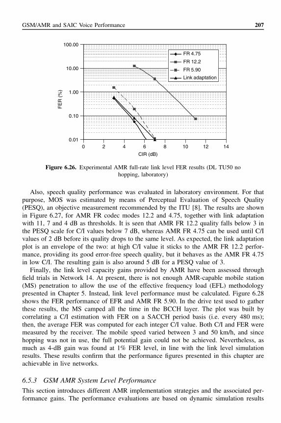
Extensive laboratory and field validation of the simulated results presented previouslyhas been conducted. The results for a TU50 non-hopping channel profile are shown inthe following figures. Figure 6.26 shows the FER performance of AMR FR codec modes12.2, 5.90 and 4.75, together with link adaptation (using codecs 12.2, 7.40, 5.90 and4.75; 11, 7 and 4 dB as thresholds). Around 6-dB gain at 1% FER is found for the linkadaptation,9 which confirms the link gains predicted in the simulations.
9 As per Figures 6.21 and 6.24, AMR FR 12.2 is used as an approximation of EFR in this subsection. Theassumption is pessimistic in terms of speech quality.
GSM/AMR and SAIC Voice Performance 207
0.01
0.10
1.00
10.00
100.00
0 2 4 6 8 10 12 14
CIR (dB)
FE
R (
%)
FR 4.75
FR 12.2
FR 5.90
Link adaptation
Figure 6.26. Experimental AMR full-rate link level FER results (DL TU50 nohopping, laboratory)
Also, speech quality performance was evaluated in laboratory environment. For thatpurpose, MOS was estimated by means of Perceptual Evaluation of Speech Quality(PESQ), an objective measurement recommended by the ITU [8]. The results are shownin Figure 6.27, for AMR FR codec modes 12.2 and 4.75, together with link adaptationwith 11, 7 and 4 dB as thresholds. It is seen that AMR FR 12.2 quality falls below 3 inthe PESQ scale for C/I values below 7 dB, whereas AMR FR 4.75 can be used until C/Ivalues of 2 dB before its quality drops to the same level. As expected, the link adaptationplot is an envelope of the two: at high C/I value it sticks to the AMR FR 12.2 perfor-mance, providing its good error-free speech quality, but it behaves as the AMR FR 4.75in low C/I. The resulting gain is also around 5 dB for a PESQ value of 3.
Finally, the link level capacity gains provided by AMR have been assessed throughfield trials in Network 14. At present, there is not enough AMR-capable mobile station(MS) penetration to allow the use of the effective frequency load (EFL) methodologypresented in Chapter 5. Instead, link level performance must be calculated. Figure 6.28shows the FER performance of EFR and AMR FR 5.90. In the drive test used to gatherthese results, the MS camped all the time in the BCCH layer. The plot was built bycorrelating a C/I estimation with FER on a SACCH period basis (i.e. every 480 ms);then, the average FER was computed for each integer C/I value. Both C/I and FER weremeasured by the receiver. The mobile speed varied between 3 and 50 km/h, and sincehopping was not in use, the full potential gain could not be achieved. Nevertheless, asmuch as 4-dB gain was found at 1% FER level, in line with the link level simulationresults. These results confirm that the performance figures presented in this chapter areachievable in live networks.
6.5.3 GSM AMR System Level PerformanceThis section introduces different AMR implementation strategies and the associated per-formance gains. The performance evaluations are based on dynamic simulation results

208 GSM, GPRS and EDGE Performance
0.0
0.5
1.0
1.5
2.0
2.5
3.0
3.5
4.0
0 2 4 6 8 10 12 14 16
CIR (dB)
PE
SQ
FR 4.75
FR 12.2
Link adaptation
Figure 6.27. Experimental AMR full-rate link level speech quality results (DL TU50 nohopping, laboratory)
−5
102
101
100
10−1
10−2
C/l (dB)
Averaged FER versus C/l
Ave
rage
FE
R (
%)
200 5 10 15
AMREFR
Figure 6.28. Experimental AMR full-rate link level FER results (DL TU50 no hopping,real network)
GSM/AMR and SAIC Voice Performance 209
and in most cases refer to the performance of RF hopping configurations. Also, fieldtrial results are provided to back up simulations. The BCCH performance is evaluatedseparately.
In the mixed traffic case (EFR and AMR capable terminals), two deployment strate-gies are studied. The first one deploys AMR in a single hopping layer and achieves itsgains with the use of more aggressive PC settings for AMR mobiles, thus decreasingthe interference level in the network. Owing to better error correction capability againstchannel errors, lower C/I targets can be set for AMR mobiles; hence tighter PC thresholdscan be used. Another deployment strategy would be to make use of the reuse partitioningtechniques to distribute the traffic across the layers according to the terminals’ capabilities.
The use of HR channel mode is potentially an efficient way to increase capacity andHW utilisation in the network. However, when using HR codec modes, the connectionsrequire higher C/I in order to achieve the same quality as AMR FR, as displayed inFigure 6.23. Therefore, in order to determine the performance and resource utilisationcapabilities of HR channel mode, a careful analysis is needed.
6.5.3.1 Codec Mode Adaptation
The codec mode adaptation for AMR is based on received channel quality estimation.The GSM specifications [7] include a reference adaptation algorithm based on C/I. In thismethod, the link quality is estimated by taking burst level C/I samples. Then, samples areprocessed using non-adaptive Finite Impulse Response (FIR) filters of order 100 for FRand 50 for HR channels. The described C/I-based quality evaluation method was used inthe codec mode adaptation simulations in this study. The target of these simulations wasto demonstrate the effect of codec mode adaptation in the system level quality and tofind out optimum thresholds for subsequent performance simulations. Table 6.1 definesthe C/I thresholds used in the codec mode adaptation simulations.
The GSM specifications [7] define that a set of up to four AMR codec modes, whichis selected at call set-up, is used during the duration of the call (the codec set can beupdated at handover or during the call). The set of codec modes presented in Table 6.2was included in the following performance evaluation simulations. In order to utilisethe total dynamic range that AMR codec offers, the lowest 4.75 kbps and the highest12.2 kbps modes were chosen in this set.
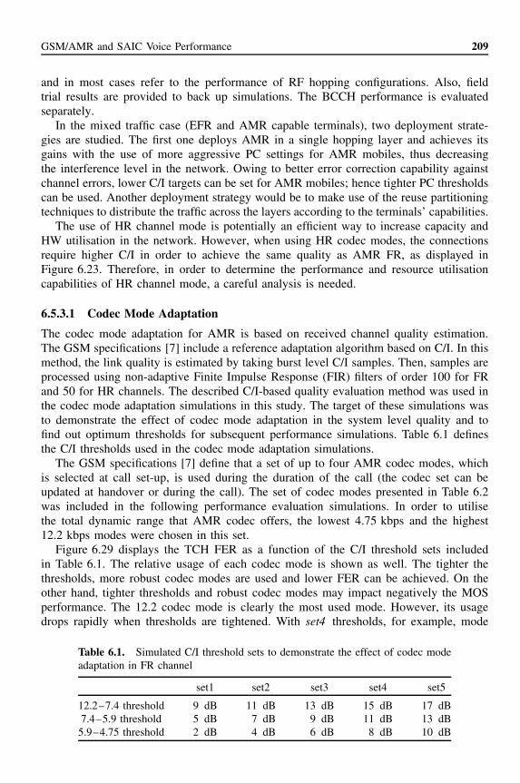
Figure 6.29 displays the TCH FER as a function of the C/I threshold sets includedin Table 6.1. The relative usage of each codec mode is shown as well. The tighter thethresholds, more robust codec modes are used and lower FER can be achieved. On theother hand, tighter thresholds and robust codec modes may impact negatively the MOSperformance. The 12.2 codec mode is clearly the most used mode. However, its usagedrops rapidly when thresholds are tightened. With set4 thresholds, for example, mode
Table 6.1. Simulated C/I threshold sets to demonstrate the effect of codec modeadaptation in FR channel
set1 set2 set3 set4 set5
12.2–7.4 threshold 9 dB 11 dB 13 dB 15 dB 17 dB7.4–5.9 threshold 5 dB 7 dB 9 dB 11 dB 13 dB
5.9–4.75 threshold 2 dB 4 dB 6 dB 8 dB 10 dB

210 GSM, GPRS and EDGE Performance
Table 6.2. Defined mode setsfor the performance simulations
AMRfull-rate set
(kbps)
AMRhalf-rate set
(kbps)
12.27.4 7.45.9 5.94.75 4.75
100
0
10
20
30
40
50
60
70
80
90
Set5Set4Set3Set2Set1
Tighter thresholds
Mod
e us
age
(%)
1.0
0.9
0.8
0.7
0.6
0.5
0.4
0.3
0.2
0.1
0.0
FE
R (
%)
% FR 12.2
% FR 7.40
% FR 5.90
% FR 4.75
AverageFER (%)
Figure 6.29. Average TCH FER and mode usage for different settings
12.2 is used less than 50% of the time and the usage of the mode 4.75 has increased over10%. In order to find out the threshold settings with best speech quality performance, anMOS evaluation is needed.
Figure 6.30 displays a MOS performance analysis for the different threshold settings.The metrics used are the percentage of bad quality connections; a connection is con-sidered as bad quality if its average MOS is below 3.2. In the system simulator, theMOS of the ongoing connections can be estimated by mapping the measured TCHFER values to corresponding MOS values. MOS values presented in [6] were used inthis mapping. It can be seen that the best performing setting is set3, even though itsaverage FER is higher than set4 and set5. As explained in this section, the selectionof the optimum thresholds will ensure that the AMR codec MOS performance followsthe envelope of the ideal codec mode adaptation, that is, the best performing codec isalways used. In the following simulations, the codec mode usage distributions are notpresented, but this example gives the typical proportions likely to be seen in differentAMR configurations.

GSM/AMR and SAIC Voice Performance 211
0
1
2
3
4
5
6
7
8
Set1 Set2 Set3 Set4 Set5Tighter thresholds
Con
nect
ion
MO
S <
3.2
(%)
Figure 6.30. MOS performance as a function of threshold tightening
6.5.3.2 Single-layered Scenario Deployment
The previous section showed the speech quality increase accomplished with the AMRcodec. There are several possibilities to turn this increased quality into additional capacityin the network. Naturally, if there were only AMR mobiles in the network, the networkcapacity could be easily increased by using tighter frequency reuses. However, mostpractical cases will have a mixture of AMR and non-AMR capable terminals in thenetwork. In the mixed traffic scenario, one way to obtain the AMR gains would be throughthe adjustment of the PC settings so that AMR connections generate less interference.This can be effectively done defining different PC thresholds for AMR and non-AMRmobiles. The use of tighter PC thresholds for AMR mobiles will effectively lower thetransmission powers used and therefore less interference will be generated. The followingnetwork simulations present the performance results using this technique.
Figure 6.31 displays the simulation results for a single-layered hopping network, withdifferent AMR terminal penetration, and different PC thresholds for EFR and AMR traffic.Performance was measured in terms of FER. The number of bad FER samples using a 2 saveraging window was calculated. Samples with FER higher than 4.2% were consideredbad quality samples. The use of AMR has a major impact on the system quality for thesame traffic load. On the other hand, the use of AMR increases substantially the networkcapacity for the same quality criteria. Figure 6.32 illustrates the relative capacity gains fordifferent AMR penetrations compared to the EFR traffic case. There is more than 50%capacity gain with 63% AMR penetration, and up to 150% capacity increase in the caseof full AMR penetration.
Since different speech codecs have different MOS performance, it is important toanalyse the MOS-based performance of AMR. Figure 6.33 shows that the AMR MOS-based gain is close as well to 150%. The calculation of MOS in network level simulatorsis estimative only, and assumptions must be made. From this analysis, it can be statedthat MOS gain is in the same range as FER gain, as expected from the link level results

212 GSM, GPRS and EDGE Performance
0.0
0.5
1.0
1.5
2.0
2.5
3.0
3.5
4.0
4.5
0 5 10 15 20 25 30
Effective frequency load (%)
Bad
TC
H F
ER
sam
ples
(%
)0% AMR/100% EFR
25% AMR/75% EFR
63% AMR/37% EFR
100% AMR/0% EFR
150%
Capacity gain
Quality gain
Figure 6.31. Single-layer AMR FER performance
0
20
40
60
80
100
120
140
160
0 20 40 60 80 100
AMR penetration (%)
Cap
acity
gai
n (%
)
Figure 6.32. TCH FER-based AMR capacity gain
presented in the previous section, where similar gains were pointed out for FER- andMOS-based link performance.
These results assume a good performance link adaptation. Nevertheless, the core ofthe algorithm itself is not specified in the standards, and its implementation is challeng-ing, mostly in terms of the C/I estimation and fading compensation [7]. Non-ideal linkadaptation in the MS can impact the overall capacity gain in the DL direction. However,this is heavily MS-dependant, and for the reference case that has been studied here, it canbe concluded that the gain of AMR with full terminal penetration on top of the definedGSM baseline performance is around 150%, both in terms of FER and MOS.

GSM/AMR and SAIC Voice Performance 213
0
1
2
3
4
5
6
0 5 10 15 20 25 30 35
Effective frequency load (%)
Con
nect
ion
MO
S <
3.2
(%
)
0% AMR/100% EFR
25% AMR/75% EFR
63% AMR/37% EFR
100% AMR/0% EFR
Capacity gain
~150%
Figure 6.33. MOS-based AMR capacity gain
6.5.3.3 Multiple Layered Scenario Deployment
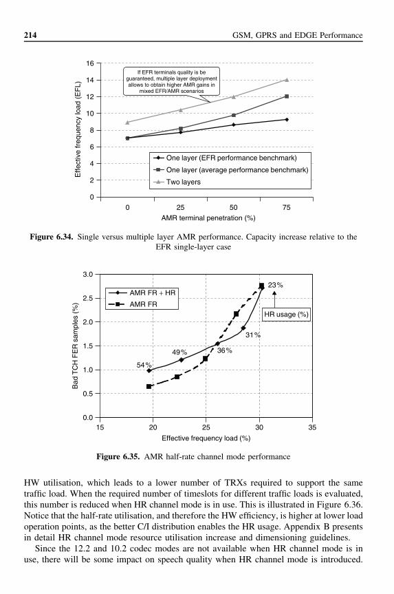
The use of the AMR functionality, together with reuse partitioning techniques, allows thenetwork performance in the mixed traffic scenario to be further increased. AMR mobilescan be handed over to the underlay layer, which deploy tighter reuses, while the non-AMR mobiles would stay in the overlay layer where the looser reuses guarantee adequateperformance. In Figure 6.34, the performance of the simulated multiple layer network iscompared with the single-layer network. In the single-layer case, if the quality of theEFR connections is to be guaranteed, the potential AMR gains cannot be realised. In themultiple layer scenario, the AMR gains are realised and at the same time the quality ofEFR connections guaranteed. This is translated to the slopes of the capacity increasesdisplayed in the figure.
6.5.3.4 Half-rate Channel Mode
The MOS performance evaluation presented in this section demonstrated that AMR HRchannel mode can be used without any noticeable speech quality degradation in high C/Iconditions, since the HR channel mode uses the same set of speech codecs as the FRmode. In order to efficiently deploy HR, it is essential to have a quality-based channelmode adaptation algorithm that selects the adequate (good quality) to change from FR toHR. In the following simulations, the channel mode adaptation was based on the measuredRXQUAL values. All incoming calls were first allocated to FR channel, and after a qualitymeasurement period, it was decided whether the connection continues in FR mode or achannel mode adaptation is performed.
The effect of AMR HR utilisation on the FER-based performance is illustrated inFigure 6.35. Both AMR FR only and AMR FR and HR have similar performance. In otherwords, the use of HR neither improves nor degrades the overall network performance interms of spectral efficiency. The gain from AMR HR channel mode comes from the higher
214 GSM, GPRS and EDGE Performance
0
2
4
6
8
10
12
14
16
0 25 50 75
AMR terminal penetration (%)
Effe
ctiv
e fr
eque
ncy
load
(E
FL)
One layer (EFR performance benchmark)
One layer (average performance benchmark)
Two layers
If EFR terminals quality is beguaranteed, multiple layer deploymentallows to obtain higher AMR gains in
mixed EFR/AMR scenarios
Figure 6.34. Single versus multiple layer AMR performance. Capacity increase relative to theEFR single-layer case
0.0
0.5
1.0
1.5
2.0
2.5
3.0
15 20 25 30 35
36%
31%
23%
49%
Effective frequency load (%)
Bad
TC
H F
ER
sam
ples
(%)
54%
HR usage (%)
AMR FR + HR
AMR FR
Figure 6.35. AMR half-rate channel mode performance
HW utilisation, which leads to a lower number of TRXs required to support the sametraffic load. When the required number of timeslots for different traffic loads is evaluated,this number is reduced when HR channel mode is in use. This is illustrated in Figure 6.36.Notice that the half-rate utilisation, and therefore the HW efficiency, is higher at lower loadoperation points, as the better C/I distribution enables the HR usage. Appendix B presentsin detail HR channel mode resource utilisation increase and dimensioning guidelines.
Since the 12.2 and 10.2 codec modes are not available when HR channel mode is inuse, there will be some impact on speech quality when HR channel mode is introduced.

GSM/AMR and SAIC Voice Performance 215
25.93% 23.33%18.18% 17.14% 16.67% 15.38%
0
5
10
15
20
25
30
35
40
45
19.56 22.25 24.93 26.91 27.85 30.20
Effective frequency load (%)
2%
blo
ckin
g re
quire
d nu
mbe
r of
TS
Ls
0
10
20
30
40
50
60
70
80
90
100
% T
SL
save
d w
ith H
R c
hann
el m
ode% of saved TSLs
Number of TSLs required for AMR FRNumber of TSLs required for AMR FR + HR
Figure 6.36. Half-rate gain in terms of timeslot requirements
0
10
20
30
40
50
60
70
80
90
100
−1.5 −1.3 −1.1 −0.9 −0.7 −0.5 −0.3 −0.1
MOS decrease
Cum
ulat
ive
dist
ribut
ion
(%) AMR FR
AMR FR + HR~0.2 MOS decrease
due to HR usage
Figure 6.37. HR channel mode impact on MOS performance
Figure 6.37 presents the speech quality distribution of the connections as a function ofMOS degradation, where the reference is EFR speech quality in error-free conditions.There is only an additional 0.2 MOS degradation when AMR HR channel mode is usedwhich is due to the unavailability of the high AMR speech codecs (12.2 and 10.2) in theHR channel mode.
Finally, the use of AMR HR channel mode requires fewer TRXs for the same trafficload so the effective deployed reuse is looser. Looser reuses have some positive perfor-mance side effects such as higher MAIO management control, and higher performancegains in case dynamic frequency and channel allocation (DFCA) (Chapter 9) is intro-duced. Therefore, the introduction of HR channel mode reduces the TRX configurationand indirectly increases the performance.
216 GSM, GPRS and EDGE Performance
6.5.3.5 AMR Codec Performance in BCCH Frequencies
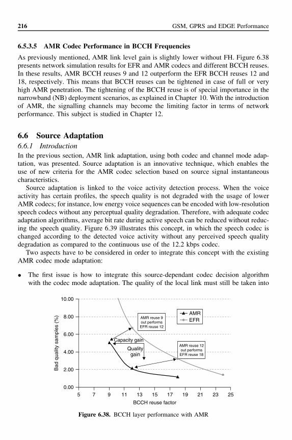
As previously mentioned, AMR link level gain is slightly lower without FH. Figure 6.38presents network simulation results for EFR and AMR codecs and different BCCH reuses.In these results, AMR BCCH reuses 9 and 12 outperform the EFR BCCH reuses 12 and18, respectively. This means that BCCH reuses can be tightened in case of full or veryhigh AMR penetration. The tightening of the BCCH reuse is of special importance in thenarrowband (NB) deployment scenarios, as explained in Chapter 10. With the introductionof AMR, the signalling channels may become the limiting factor in terms of networkperformance. This subject is studied in Chapter 12.
6.6 Source Adaptation6.6.1 IntroductionIn the previous section, AMR link adaptation, using both codec and channel mode adap-tation, was presented. Source adaptation is an innovative technique, which enables theuse of new criteria for the AMR codec selection based on source signal instantaneouscharacteristics.
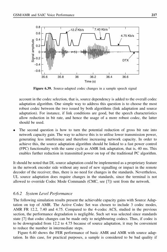
Source adaptation is linked to the voice activity detection process. When the voiceactivity has certain profiles, the speech quality is not degraded with the usage of lowerAMR codecs; for instance, low energy voice sequences can be encoded with low-resolutionspeech codecs without any perceptual quality degradation. Therefore, with adequate codecadaptation algorithms, average bit rate during active speech can be reduced without reduc-ing the speech quality. Figure 6.39 illustrates this concept, in which the speech codec ischanged according to the detected voice activity without any perceived speech qualitydegradation as compared to the continuous use of the 12.2 kbps codec.
Two aspects have to be considered in order to integrate this concept with the existingAMR codec mode adaptation:
• The first issue is how to integrate this source-dependant codec decision algorithmwith the codec mode adaptation. The quality of the local link must still be taken into
Qualitygain
0.00
2.00
4.00
6.00
8.00
10.00
5 252321191715131197
BCCH reuse factor
Bad
qua
lity
sam
ples
(%
) AMREFR
AMR reuse 12out performsEFR reuse 18
AMR reuse 9out performsEFR reuse 12
Capacity gain
Figure 6.38. BCCH layer performance with AMR
GSM/AMR and SAIC Voice Performance 217
35.6 35.8 36 36.2 36.4 36.6
−0.6
−0.4
−0.2
0
0.2
0.4
0.6
0.8
Time (s)
Sig
nal a
mpl
itude
4.75 Kb/s
DTX
7.40 Kb/s12.2 Kb/s
Figure 6.39. Source-adapted codec changes in a sample speech signal
account in the codec selection, that is, source dependency is added to the overall codecadaptation algorithm. One simple way to address this question is to choose the mostrobust codec between the two issued by both algorithms (link adaptation and sourceadaptation). For instance, if link conditions are good, but the speech characteristicsallow reduction in bit rate, and hence the usage of a more robust codec, the lattershould be used.
• The second question is how to turn the potential reduction of gross bit rate intonetwork capacity gain. The way to achieve this is to utilise lower transmission power,generating less interference and therefore increasing network capacity. In order toachieve this, the source adaptation algorithm should be linked to a fast power control(FPC) functionality with the same cycle as AMR link adaptation, that is, 40 ms. Thisenables further reduction in transmitted power on top of the traditional PC algorithm.
It should be noted that DL source adaptation could be implemented as a proprietary featurein the network encoder side without any need of new signalling or impact in the remotedecoder of the receiver; thus, there is no need for changes in the standards. Nevertheless,UL source adaptation does require changes in the standards, since the terminal is notallowed to override Codec Mode Commands (CMC, see [7]) sent from the network.
6.6.2 System Level Performance
The following simulation results present the achievable capacity gains with Source Adap-tation on top of AMR. The Active Codec Set was chosen to include 3 codec modes,AMR FR 12.2, 7.40 and 4.75. Compared to the 4-codec ACS, studied in the previoussection, the performance degradation is negligible. Such set was selected since standardsstate [7] that codec changes can be made only to neighbouring codecs. Thus, if codec isto be downgraded from 12.2 to 4.75 because of source adaptation, it may be convenientto reduce the number in intermediate steps.
Figure 6.40 shows the FER performance of basic AMR and AMR with source adap-tation. In this case, for practical purposes, a sample is considered to be bad quality if

218 GSM, GPRS and EDGE Performance
FER performance, AMR versus AMR + SA
0.0
0.5
1.0
1.5
2.0
2.5
15 20 25 30 35
Effective frequency load (%)
Bad
TC
H F
ER
(>2
%)
sam
ples
(%
)
AMR AMR + SA
Figure 6.40. Performance of source adaptation compared to AMR
0.0
10.0
20.0
30.0
40.0
50.0
60.0
70.0
80.0
FR 12.2 (%) FR 7.40 (%) FR 4.75 (%)
Cod
ec u
sage
(%
)
Source adaptation AMR (no source adaptation)
Figure 6.41. Mode usage with and without source adaptation

GSM/AMR and SAIC Voice Performance 219
its FER is higher than 2%. From these simulations, a gain of 25% is achieved with theintroduction of source adaptation.
As explained in the previous sections, this gain is basically due to a reduction in thetransmitted power (FPC function), which is made possible because of the usage of morerobust codecs. This effect is illustrated in Figure 6.41, where a comparison between codecdistributions with and without source adaptation is shown. It can be seen that the usageof AMR FR 12.2 is reduced from 70% to almost 40%, whereas AMR FR 4.75 usageis increased from 10% to around 35%. As stated before, this bit-rate reduction does notimpact perceived quality.
6.7 Rel’5 EDGE AMR Enhancements6.7.1 Introduction
This section presents the performance analysis of the AMR enhancements included inRel’5 and presented in Chapter 2.
GERAN Rel’5 specifies a new octagonal phase shift keying (8-PSK) modulated HRchannel mode (O-TCH/AHS) for AMR NB speech. This new physical channel allowsthe use of all the available NB AMR speech codecs, with code rates ranging from 0.14(AMR4.75) to 0.36 (AMR12.2).
Additionally, Rel’5 brings one additional method to increase the speech capacity ofthe network. A new Enhanced Power Control (EPC) method can be used for dedicatedchannels with both Gaussian minimum shift keying (GMSK) and 8-PSK modulation.10
EPC steals bits from the SACCH L1 header to be used for measurement reports (uplink)and PC commands (downlink). This way the PC signalling interval can be reduced fromSACCH block level (480 ms) down to SACCH burst level (120 ms). Thanks to optimisedchannel coding scheme (40-bit FIRE code replaced with 18-bit CRC code) of the newSACCH/TPH channel, the link level performance is actually improved by 0.6 dB (TU3ideal FH at 10% BLER). See Reference [9] for further details.
This section also describes a major speech quality enhancement feature of Rel’5, theintroduction of the WB AMR speech codecs. Link level results for WB-AMR in bothGMSK FR and 8-PSK HR channels are presented.
6.7.2 EDGE NB-AMR Performance
Figure 6.42 displays the link level performance of the new 8-PSK Half-Rate channels,which is better than the performance of GMSK channels for all the AMR codec modesexcept for the most robust one (4.75 kbps). The higher the AMR codec mode is, the betterthe O-TCH/AHS channel mode performs compared to the TCH/AHS mode.
Listening tests (33 listeners, clean speech) were conducted in order to verify the sub-jective performance of the EDGE AMR HR channel mode compared to standard GSMAMR HR. Figure 6.43 presents the collected results. At each operating point (C/I), theAMR mode with highest MOS value is selected. The results show a clear benefit forthe EDGE AMR HR over GSM AMR HR. Owing to the higher AMR modes in EDGE,
10 Note that this is not the same as fast power control (FPC), which is specified for ECSD in Rel’99. ECSDFPC uses a 20-ms signalling period.

220 GSM, GPRS and EDGE Performance
0.10
1.00
10.00
100.00
0 2 4 6 8 10 12 14 16 18
CIR (dB)
FE
R (
%)
O-TCH/AHS 12.2TCH/AHS 7.4O-TCH/AHS 7.4TCH/AHS 5.9O-TCH/AHS 5.9O-TCH/AHS 4.75TCH/AHS 4.75
Figure 6.42. Link level performance of main TCH/AHS and O-TCH/AHS codec modes. TU3iFH channels
0
1
2
3
4
5
6 18161412108
C/l (dB)
MO
S
AMR 4.75
AMR 5.15
AMR 6.7 AMR 7.95AMR 5.9
AMR 6.7AMR 7.95 AMR 12.2
O-TCH/AHSTCH/AHS
Figure 6.43. Comparison of MOS test results between GSM AMR and EDGE AMR half-rate.Best codec is selected for each operating point
the subjective performance gains would be even higher in typical practical conditions,where C/I is high and background noise is present.
From all these results, it can be concluded that EDGE AMR HR channel should beprioritised over GSM AMR HR channel, that is, when EDGE AMR HR is available, thereis no need to do channel mode adaptation to GSM AMR HR. This is mainly because ofthe possibility to also use the two highest AMR codec modes (10.2 and 12.2).
Network simulations have confirmed the expected results from the above presented linklevel performance. Although no significant differences in terms of FER are observed when

GSM/AMR and SAIC Voice Performance 221
0
10
20
30
40
50
60
70
80
90
100
−1.5 −1.3 −1.1 −0.9 −0.7 −0.5 −0.3 −0.1
MOS decrease
Cum
ulat
ive
dist
ribut
ion
(%) AMR FR + EAMR HR
AMR FR + AMR HR ~0.2 MOS increasewith EAMR
Figure 6.44. O-TCH/AHS channel mode impact on MOS performance
0
10
20
30
40
50
60
70
80
90
100
FR 12.2 FR 7.40 FR 5.90 FR 4.75 HR 12.2 HR 7.40 HR 5.90 HR 4.75
Mod
e us
age
with
in c
hann
el m
ode
(%)
AMR FR + AMR HR
AMR FR + EAMR HR
Figure 6.45. Mode usage when using O-TCH/AHS and TCH/AHS
using O-TCH/AHS, there is certainly an increase in the average speech quality perceivedby the end-user, which is shown in Figure 6.44. In this figure, both plots correspond tothe use of Codec and Channel Mode adaptation, but in ‘AMR FR-HR’ HR modulationis GMSK (as in Section 6.5.3.4), whereas in ‘E-AMR’ HR modulation is 8-PSK, addingthe 12.2 kbps codec. The figure shows the quality distribution of the connections as afunction of MOS degradation, in a way similar to Figure 6.37. The speech quality gainis roughly 0.2 on the MOS scale.
Figure 6.45 shows the compared codec mode usage histograms. FR codecs remain prac-tically the same, but the presence of the additional 12.2 kbps codec in the O-TCH/AHS

222 GSM, GPRS and EDGE Performance
alters the HR distribution significantly. Almost 70% of the time an 8-PSK HR channel isused, the 12.2 kbps codec will be selected. It is the high usage of this codec that providesspeech quality improvement. The final conclusion then is that although E-AMR NB doesnot provide significant capacity gains, it increases the average speech quality.
6.7.3 EPC Network Performance
The faster PC cycle of EPC can be transformed into system capacity gain. This gaindepends heavily on the mobile station speed and shadow-fading component of the signal.An extensive set of network level simulations were performed in order to study the effectof EPC on system level. The simulation set-up was similar to the one used in the basicGSM HR simulations presented earlier. Only non-BCCH layer was studied with 1/1 RFhopping and 4.8 MHz of total spectrum. DTX was not used and bad quality call criteriawas 1% FER averaged over the whole call. In the simulations, the EPC performancewas compared to the standard PC performance, using the same RxQual/RxLev-based PCalgorithm. Figure 6.46 shows the performance results at different speeds and shadow-fading profiles.
These results show that the gain from EPC is substantial for fast moving mobiles(around 20%) but quite small in the case of slow moving mobiles (the relative gain ofEPC increases slightly also when the slow-fading variation is higher). This points out thesufficient speed of the GSM standard PC mechanism to follow shadow-fading variationsfor slow moving mobiles.
6.7.4 EDGE Wideband AMR Codecs
GERAN Rel’5 specifies new AMR WB speech codecs, which present a major improve-ment in speech quality. With the introduction of a new 8-PSK FR physical channel, WBAMR modes up to 23.85 kbps can be supported. The highest modes offer performanceexceeding standard wireline quality. Owing to improved speech coding, WB codecs offerbetter quality than NB codecs even with similar codec bit rates. WB AMR codec modesin Rel’5 are defined for GMSK FR (TCH/WFS) and for 8-PSK FR (O-TCH/WFS) andHR (O-TCH/WHS). The usage of GMSK HR with WB codecs has not been standardised.
0
2
4
8
6
10
4 1412119865 13107
EFL (%)
Bad
qua
lity
calls
(%
) 3 km/hEPC-3 km/h
EPC-50 km/h50 km/h
0
2
4
8
6
10
2 111097643 85
EFL (%)
Bad
qua
lity
calls
(%
)
3 km/hEPC-3 km/h
50 km/hEPC-50 km/h
Figure 6.46. TCH-AHS EPC performance for slow fading standard deviation of 6 and 8 dB

GSM/AMR and SAIC Voice Performance 223
Three codec modes are available in all channels: 12.65, 8.85 and 6.60 kbps. For 8-PSKFR channels (O-TCH/WFS), two additional WB-AMR codec modes can be used: 23.85and 15.85, which offer very high quality speech in good channel conditions.
Figure 6.47 (a) shows the link level performance of WB AMR codecs on the GMSKFR (TCH/WFS) and 8-PSK HR (O-TCH/WHS) channels. The C/I requirements for 1%FER are between 5 and 9 dB for GMSK and about 4 dB higher with 8-PSK. Figure 6.47(b) shows the curves for 8-PSK FR. The C/I requirement range for the three lowest modesis now between 4 and 6 dB.
Finally, Figure 6.48 summarises the C/I requirements of all the modes. It can be con-cluded that especially the 8-PSK FR channels seems to provide a very attractive optionto provide truly high quality speech without compromising capacity.
0.1
1.0
10.0
100.0
0 2 4 6 8 10 12 14 16
C/I (dB)
FE
R (
%)
0.1
1.0
10.0
100.0
0 2 4 6 8 10 12 14 16
C/I (dB)
(a) (b)
FE
R (
%)
O-TCH/WHS 12.65O-TCH/WHS 8.85O-TCH/WHS 6.6TCH/WFS 12.65TCH/WFS 8.85TCH/WFS 6.6
O-TCH/WFS 23.85O-TCH/WFS 15.85O-TCH/WFS 12.65O-TCH/WFS 8.85O-TCH/WFS 6.6
Figure 6.47. Link level performance of O-TCH/WHS, TCH/WFS and O-TCH/WFS AMR modes(TU3 iFH)
0
2
4
6
8
10
12
14
23.85 15.85 12.65 8.85 6.60
AMR mode
C/I
@ 1
% F
ER
O-TCH/WFSTCH/WFSO-TCH/WHS
Figure 6.48. C/I requirement for 1% FER for all WB-AMR modes (TU3iFH)

224 GSM, GPRS and EDGE Performance
6.8 Single Antenna Interference Cancellation (SAIC)SAIC is a generic term comprising several different single antenna receiver techniques,which attempt to cancel interference through signal processing. It is mainly intended forusage in the downlink, since terminal size, cost and aesthetics requirements preclude theusage of multiple antenna techniques.
Within the 3GPP standardisation work carried out by Technical Specification Group(TSG) GERAN, an SAIC feasibility study is currently ongoing, investigating the expectedperformance of SAIC terminals in typical network scenarios and the need for signallingof the MS SAIC capability, for example, by using the MS classmark information.
The goal is to have SAIC standardised for Rel’6. However, owing to some operators’requests to have SAIC terminals earlier than Rel’6 natural timeframe, SAIC could becomea release-independent functionality, with the first commercial terminals available in early2004. This section attempts to explain the current status of the SAIC development, andanalyse it in terms of link and network performance enhancements.
6.8.1 SAIC Techniques OverviewIn GSM, one of the main factors limiting the spectral efficiency is the MS receiverperformance when subject to co-channel interference (CCI). Conventional receivers havetraditionally been optimised for Gaussian noise; nevertheless, as the nature of interferenceis partly known (e.g. modulation type and its subsequent characteristics, training sequence,etc), it is possible to optimise receivers to improve the performance in the presence ofsuch interference. For mobiles having a single antenna, a number of techniques exist, allbeing designated as SAIC. Although SAIC techniques can be applied for both CCI andAdjacent Channel Interference (ACI), the main focus in this section will be SAIC forsuppression of CCI.
In the literature, a number of SAIC techniques exist but basically they can be dividedinto two families:
• Joint Detection/Demodulation (JD)• Blind Interference Cancellation (BIC)
The basic principle of Joint Detection [10, 11] is to do simultaneous detection of thedesired and the interfering signal. In order to do this, JD methods rely on the identificationof Training Sequence Code (TSC) of the interferer and its offset from the TSC of thedesired signal. On this basis, a joint channel estimation is conducted using the 26 knownbits from the interfering TSC and the corresponding bits from the desired signal. Theresulting refined channel estimate takes into account the effect of the interfering burst,which improves the accuracy of the estimate and thereby decreases the BER. The twochannel estimates are then used in a joint detector, which simultaneously detects thedesired and the interfering signal.
JD works for both GMSK and 8-PSK modulations, although simulations have demon-strated that the best performance is achieved for a GMSK-modulated interferer. BecauseJD detects simultaneously the desired and the interfering signal, its performance is gener-ally superior to other cancellation techniques, although at the cost of higher complexity.
Compared with JD, BIC techniques do not explicitly need a channel estimate of theinterfering signal to perform detection of the desired signal. Several BIC methods exist,

GSM/AMR and SAIC Voice Performance 225
using different properties of the interfering signal; for example, for a GMSK-modulatedinterferer it is possible to use its constant envelope property or the fact that the sameinformation is carried in the real and imaginary part of the signal [12, 13]. Basically,BIC techniques have a lower complexity than JD-based methods, making them morecost efficient and therefore attractive for first-generation SAIC terminals. The cost forthis lower complexity is a reduction in the potential performance gain, compared withmethods based on JD. The SAIC results presented in this section are based on twodifferent low complexity BIC solutions: the first one is Mono Interference Cancellation(MIC) [13]; the other is called GMSK-IC (Interference Cancellation). Both the solutionshave previously been used to generate input to the feasibility study ongoing in TSGGERAN [14, 15].
Identification of SAIC capability is another important issue currently being debated.The network is likely to require the knowledge of which mobiles are SAIC-capable, andpotentially to what degree (e.g. GMSK only, GMSK and 8-PSK, etc). Such informationmay be beneficial for the network to control the C/I conditions different terminals aresubject to: for instance, through tighter effective reuses for SAIC MS, or by means ofSAIC-optimised Power Control, or even SAIC-tuned DFCA algorithms (see Chapter 9).Several possibilities exist: special signalling could be defined (one way to do this is to haveexplicit classmark information) or the network could be required to identify SAIC-capableterminals in an unassisted way.
6.8.2 SAIC Link Performance and Conditioning FactorsSAIC receivers are, as explained in the last section, optimised to extract additional infor-mation from the incoming signals to improve the detection of the desired signal. Asa consequence, the performance of SAIC receivers can generally have large variations,depending on different parameters. The three most important parameters affecting SAICreceiver performance are the delay between desired and interfering signal, their respectiveTSC, and finally a new parameter named Dominant to rest of Interference Ratio (DIR).Each algorithm behaves differently with respect to these variables, and this makes thecharacterisation of SAIC performance a challenging task.
Delays, especially between the main interferer and the desired signal, affect the perfor-mance of SAIC mobiles. Especially for implementations based on JD such delays can becritical, resulting in a significant drop in performance gains already at 5-symbols delay.BIC techniques are generally not so sensitive to delays and some algorithms can havea nearly constant gain with up to 20 symbols delay. This means that achievement ofmaximum SAIC benefits, especially in the case of JD, requires synchronised networks,which guarantee low delays between desired and interfering signals. In such a case, aninter-site distance of 3 km would imply an approximate maximum possible delay of 4symbols,11 and a median value much below that figure. Figure 6.49 [16] shows somelaboratory results using a SAIC prototype, where the performance for different delaysbetween desired signal and a single interferer has been tested. For this scenario, it canbe seen that at large delays the link level gain is 4 dB at 1% FER, which is approxi-mately half the gain that can be achieved when the interfering and desired signal are fully
11 Bit length is about 1.1 km; assuming interference comes always from first tier, maximum distance betweenMS and interferer BTS can be 4.5 km at most.
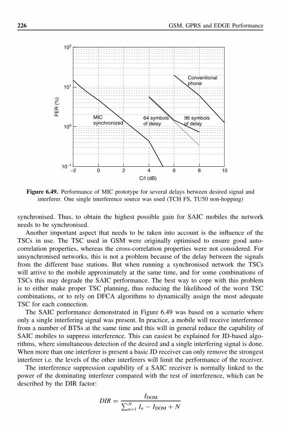
226 GSM, GPRS and EDGE Performance
10−1
100
101
102
0 2−2 4
MICsynchronized
Conventionalphone
64 symbolsof delay
96 symbolsof delay
6 8 10
C/I (dB)
FE
R (
%)
Figure 6.49. Performance of MIC prototype for several delays between desired signal andinterferer. One single interference source was used (TCH FS, TU50 non-hopping)
synchronised. Thus, to obtain the highest possible gain for SAIC mobiles the networkneeds to be synchronised.
Another important aspect that needs to be taken into account is the influence of theTSCs in use. The TSC used in GSM were originally optimised to ensure good auto-correlation properties, whereas the cross-correlation properties were not considered. Forunsynchronised networks, this is not a problem because of the delay between the signalsfrom the different base stations. But when running a synchronised network the TSCswill arrive to the mobile approximately at the same time, and for some combinations ofTSCs this may degrade the SAIC performance. The best way to cope with this problemis to either make proper TSC planning, thus reducing the likelihood of the worst TSCcombinations, or to rely on DFCA algorithms to dynamically assign the most adequateTSC for each connection.
The SAIC performance demonstrated in Figure 6.49 was based on a scenario whereonly a single interfering signal was present. In practice, a mobile will receive interferencefrom a number of BTSs at the same time and this will in general reduce the capability ofSAIC mobiles to suppress interference. This can easiest be explained for JD-based algo-rithms, where simultaneous detection of the desired and a single interfering signal is done.When more than one interferer is present a basic JD receiver can only remove the strongestinterferer i.e. the levels of the other interferers will limit the performance of the receiver.
The interference suppression capability of a SAIC receiver is normally linked to thepower of the dominating interferer compared with the rest of interference, which can bedescribed by the DIR factor:
DIR = IDOM∑Nn=1 In − IDOM + N

GSM/AMR and SAIC Voice Performance 227
−10 −8 −6 −4 −2 0 2 4 6 8 1010−3
10−2
10−1
100R
aw B
ER
(%
)
C/I (dB)
DIR = 6 dBDIR = 10 dBDIR = 20 dBDIR = 100 dB
Figure 6.50. Link performance as a function of DIR
where IDOM is the power of the dominant interferer, M is the total number of co- andadjacent channel interferers and N is the receiver noise. In Figure 6.50, the performanceof an SAIC receiver is shown for various DIR.12 In practice, the interferer scenario will bemore complicated. As expected, the gains are higher when a single interferer is dominatingbut still some gain is possible for low DIR values.13 Figure 6.51 shows a sample of atypical cumulative distribution of DIR taken from network simulations.
6.8.3 SAIC Network PerformanceThe dependency of SAIC performance with interference delay, TSC and DIR has impor-tant implications in the network performance. It is obvious from the discussion in theprevious section that higher gains can be expected in synchronised networks having goodTSC planning, especially for Joint Detection (which will lose, anyway, part of its poten-tiality even in the synchronised case, especially in large-cell areas). Nevertheless, theimplications of DIR in performance deserve more attention. It has been identified throughsimulations that the higher the load level is, the lower the DIR values are, which, asshown in Figure 6.50, leads to a reduction in the potential link and network gains fromSAIC. Figure 6.52 shows the simulated network performance of AMR FR 5.90 for a con-ventional and an SAIC receiver. The overall gain is close to 40%.14 This is lower than the
12 A simple model based on two interferers has been used for these simulations.13 In a real network, the DIR experienced by ongoing connections can vary between −5 dB to about 30 dB,and the gain provided by SAIC would change accordingly.14 Half Rate SAIC performance is likely to provide higher gains due to the more favorable associated DIRdistribution.

228 GSM, GPRS and EDGE Performance
0
0.1
0.2
0.3
0.4
0.5
0.6
0.7
0.8
0.9
1D
IRcd
f
DIR (dB)
−5 0 5 10 15 20 25 30 35 40 45
Figure 6.51. DIR cumulative distribution function for a heavily loaded hopping network
MIC SAIC performance
1.0
0.0
2.0
3.0
4.0
5.0
6.0
7.0
10 15 20 25 30 35 40 45 50 55 60
EFL (%)
Bad
TC
H F
ER
(>2
%)
sam
ples
(%
)
Ref Ref SAIC MIC
40%
Figure 6.52. SAIC FER performance
gains theoretically expected from the link performance results displayed in Figure 6.49,which is a logic consequence of the realistic DIR conditions occurring in the network.
Also, PC actually reduces the benefits of SAIC, since it decreases DIR in the network.Finally, another important factor to be taken into account is ACI. Simulations have shownthat performance degradation in the presence of ACI is higher for SAIC traffic than for

GSM/AMR and SAIC Voice Performance 229
10−4
10−3
10−2
10−1
100
101
5 10 15 20 25 30
C/I (dB)
FE
R (
%)
MIC
Conventional
~4 dB
Figure 6.53. Experimental FER performance of conventional and MIC receivers (TCH FS,random hopping over 5 frequencies)
non-SAIC. ACI implications on SAIC are under study in standardisation, but it should benoted here that ACI is much dependant on network planning, for example, it is possibleto avoid intra-site ACI if enough spectrum is available.
Nevertheless, trials conducted to assess SAIC network performance gains have demon-strated promising results. In an unsynchronised network, a C/I decrease at 10% outageof up to 2.7 dB was registered. In synchronised networks, the reported gain ranges from2–3 dB to more than 4 dB, depending on the number of interferers. Figure 6.53 (Net-work 14) shows the measured link performance of a conventional receiver and an SAICprototype operating in a synchronised test network. C/I estimates from the receiver werecorrelated with measured FER. The interference was artificially generated in five neigh-boring sectors. This explains why the gain is higher than predicted by simulations. Thisresult is, nevertheless, indicative of the important benefits achievable through SAIC.
6.9 Flexible Layer OneFlexible Layer One (FLO) was presented and explained in Chapter 2. FLO defines aparameterised, easily configurable physical layer devised to optimally support any newInternet multimedia subsystem (IMS) and the support of FLO to AMR FR codec 12.2will be studied here.
6.9.1 FLO for Circuit-switched VoiceFigure 6.54 shows how FLO Transport Channels (TrCHs) are configured to support AMR12.2 codec. Two TrCHs, labeled A and B, are required, because of different qualityrequirements of class 1a and 1b bits. On TrCH A, the transport block is 83 bits long,whereas on TrCH B, it is 163 bits long. A 6-bit CRC is attached on TrCH A to make a

230 GSM, GPRS and EDGE Performance
TCH A
83Transport blocks
TCH B
163
89Code blocks 163
177Radio frames
CCTCH
263
17724Radio packet 263
464
Payload of 4 GMSK bursts
177 263
285Encoded blocks 507
CRC attachment
Channel coding
Rate matching
TCH multiplexing
TFCI
Interleaving
Figure 6.54. AMR FR 12.2 codec encapsulated in FLO bearers
code block of 89 bits. The two code blocks are then processed through channel coding,yielding 285 coded bits for TrCH A and 507 bits for TrCH B. After rate matching, 177 bitsare left on TrCH A and 263 bits on TrCH B. Concatenation of the two radio frames resultsin a Codec Composite TrCH (CCTrCH) of 440 coded bits. The 24-bit Transport FormatCombination Indication (TFCI) is then attached to the CCTrCH, creating a 464-bit radiopacket. The radio packet is finally diagonally interleaved over eight bursts.
The requirement that the size of the radio packet is equal to the 464-bit payloadavailable on GMSK FR channels is complied with. On the other hand, the coding rate forTrCH A is 0.503 and for TrCH B 0.620, which are close to the coding rates in AMR FR12.2: 0.500 for class 1a bits and 0.5949 for class 1b bits. The small increase is mainly dueto the overhead introduced by FLO (TFCI and tail bits for the second transport channel).
Figure 6.55 compares the link-level performance of AMR FR 12.2 with the AMR 12.2over FLO in TU3 with ideal FH. As we can see, the performance difference is negligible.In both cases, 9 dB of C/I is required to reach 1% of FER. This demonstrates the abilityof the FLO architecture to produce optimised coding schemes.
6.9.2 FLO for VoIP
In Voice over Internet Protocol (VoIP), AMR frames are encapsulated in real-time protocol(RTP) packets and carried over UDP/IP. This means that an RTP/UDP/IP header is to betransmitted together with the encoded speech. The header is compressed [17] to reducethe impact of the subsequent overhead, which is as a result of 51 bits in average. For thesame speech bit rate, this overhead will obviously reduce the channel coding protection.

GSM/AMR and SAIC Voice Performance 231
0.1
1.0
10.0
100.0
0 1 2 3 4 5 6 7 8 9 10 11 12
CIR (dB)
FE
R (
%)
AMR FR 12.2
AMR 12.2 kbps over FLO
Figure 6.55. Compared link performance of AMR FR 12.2 over non-FLO and FLO radio bearers
In Rel’5, the only radio bearers that can be used for VoIP are based on the (E)GPRScoding schemes. Unfortunately, they were not designed for real-time unacknowledgeddedicated services such as VoIP, but instead optimised for non-real-time acknowledgedshared services:
• The interleaving depth is fixed to 20 ms, although a 40-ms or an 80-ms depth isallowed by the delay requirements of VoIP.
• The VoIP payload to be carried does not always exactly fit into one RLC packet. So,padding has often to be used. For instance, with VoIP AMR 10.2, MCS-3 has to beused with a padding of 40 bits.
• The RLC/MAC header contains some fields that are useless for unacknowledgeddedicated services. For instance, the uplink state flag (USF) is not needed.
With FLO, all these problems are solved, thereby improving the performance:
• The interleaving scheme can be selected at call setup.• The size of the transport blocks is negotiated and no padding is required.• The RLC/MAC header is optimised for unacknowledged dedicated services [18].
With AMR FR 12.2 taken as an example, Figure 6.56 compares the link-level performanceof VoIP in Rel’5 with the one of the same service in Rel’6 using FLO (VoIP with AMR12.2 as codec mode is called VoIP 12.2 here). In Rel’5, MCS3 (GMSK) or MCS5 (8-PSK)can be used for VoIP 12.2. With FLO, the channel coding is tailored at call setup duringwhich some freedom is allowed. FLO offers several alternatives for the channel coding: thediagonal interleaving depth can be either 40 or 80 ms, and the modulation can be GMSKor 8-PSK. The performance for each of the four combinations is shown in Figure 6.56.

232 GSM, GPRS and EDGE Performance
0.1
1.0
10.0
100.0
0 2 4 6 8 10 12 14 16 18 20
CIR (dB)
FE
R (
%)
FLO(GMSK, 40 ms)FLO(GMSK, 80 ms)EGPRS GMSK(MCS3)FLO(8PSK, 40 ms)FLO(8PSK, 80 ms)EGPRS 8PSK (MCS5)
Figure 6.56. Link performance of VoIP12.2, with and without FLO
At 1% FER, the resulting gains range between 5 and 6.6 dB. For instance, with GMSKmodulation and 80-ms diagonal interleaving, the link-level performance of VoIP 12.2 at1% FER is improved by FLO by more than 6 dB compared to Rel’5 (non-FLO), whereMCS3 is used.
Even with FLO, there is a significant loss in performance for VoIP because of overhead.Comparison of Figure 6.55 and Figure 6.56 shows a link degradation of more than 4 dBat 1% FER (80 ms interleaving, GMSK modulation).
It can be concluded that, for CS speech, FLO is capable of providing robustness similarto the one achievable with non-FLO physical layer. Also, it improves noticeably theperformance for IMS real-time services, partially overcoming the limitations of non-FLOradio bearers.
References[1] Johansen J., Vejlgaard B., Capacity Analysis of a Frequency Hopping GSM System,
M.Sc.E.E. Thesis Report, Aalborg University, Aalborg, June 1995.[2] Nielsen Thomas T., Wigard J., Performance Enhancements in a Frequency Hopping
GSM Network, Kluwer Academic Publishers, Dordrecht, 2000.[3] Wigard J., Nielsen Thomas T., Skjærris S., Mogensen P., ‘On the Influence of Dis-
continuous Transmission in a PCS1900/GSM/DCS1800 Type of Network’, VTC’99 ,Houston, 1999.
[4] Wigard J., Mogensen P., Michaelsen P. H., Melero J., Halonen T., ‘Comparisonof Networks with different Frequency Reuses, DTX and Power Control using theEffective Frequency Load Approach’, VTC2000 , Tokyo, Japan, 2000.
[5] Watanabe F., Buot T., Iwama T., Mizuno M., ‘Load Sharing Sector Cell in CellularSystems’, IEEE Proc. PIMRC’95 , 1995, pp. 547–551.
GSM/AMR and SAIC Voice Performance 233 [6] 3GPP TR 26.975 v5.0.0 Release 5: Performance Characterization of AMR
Speech Codec. [7] 3GPP TS 45.009 v5.3.0 Release 5: Link Adaptation. [8] ITU-T Recommendation P.862 (02/2001), Perceptual Evaluation of Speech Quality
(PESQ), An Objective Method for End-to-End Speech Quality Assessment of Narrowband Telephone Networks and Speech Codecs.
[9] Bellier T., Moisio M., Sebire B., ‘Speech Capacity Enhancements in the GSM/EDGE Radio Access Network (GERAN)’, ICT2002 , Beijing, China, June 23–26 2002.
[10] Giridhar K., Chari S., Shynk J. J., Gooch R. P., Artman D., ‘Joint Estimation Algorithms for Cochannel Signal Demodulation’, IEEE Proc. Int. Conf.
Communications, Geneva, Switzerland, 1993, pp. 1497–1501. [11] Ranta P. A., Hottinen A., Honkasalo Z. C., ‘Co-channel Interference Cancelling
Receiver for TDMA Mobile Systems’, Proc. IEEE Int. Conf. Communications, Seattle, WA, 1995, pp. 17–21.
[12] P. Leung, R. Berangi, Indirect Cochannel Interference Cancellation”, Wireless personal communication 2001.
[13] Method for Interference Suppression for TDMA and/or FDMA Transmission, US Patent Application Publication No. US 2002/0141437 A1, October 3 2002.
[14] 3GPP TSG GERAN#11 Tdoc GP-022892: Draft Feasibility Study on Single Antenna Interference Cancellation (SAIC) for GSM Networks (Release 6).
[15] 3GPP TSG GERAN#13 Tdoc GP-030276: SAIC Link Level Simulation Model. [16] 3GPP TSG GERAN#11 Tdoc GP-022557: Laboratory & Field Testing of SAIC for
GSM Networks. [17] RFC 3095, RObust Header Compression (ROHC). [18] 3GPP TR 45.902, Flexible Layer One. Excerpted from “GSM, GPRS and EDGE Performance , 2nd Edition” by Timo Halonen Published October 2003. For more information or to buy a copy of this book click here. << Go Back