Growth and Business Cycles - University of Minnesota

1 Department of Economics, University of Minnesota and Federal Reserve Bank of Minneapolis,Department of Economics, University of Wisconsin, and Department of Economics, Northwestern University,respectively. We thank Larry Christiano, Ed Prescott and Craig Burnside for their help, and the National ScienceFoundation for financial support.

Preliminary and IncompleteFor discussion only

Growth and Business Cycles

Larry E. Jones,

Rodolfo E. Manuelli,

Henry E. Siu 1

First Version: January 1995, This Version: March 20, 2000


2

Abstract

Our purpose in this paper is to present a class of convex endogenous growth models, and to

analyze their performance in terms of both growth and business cycle criteria. The models we

study have close analogs in the real business cycle literature. In fact, we interpret the exogenous

growth rate of productivity as an endogenous growth rate of human capital. This perspective

allows us to compare the strengths of both classes of models.

In order to highlight the mechanism that gives endogenous growth models the ability to

improve upon their exogenous growth relatives, we study models that are symmetric in terms of

human and physical capital formation -- our two engines of growth. More precisely, we analyze

models in which the technology used to produce human capital is identical to the technologies

used to produce consumption and investment goods, and in which the technology shocks in the

two sectors are perfectly correlated.

We find that endogenous growth models can generate levels of labor volatility close to

those observed in the data, as well as positively correlated growth rates of output. We also find

that these models outperform a related exogenous growth version in most dimensions.

Larry Jones Rody ManuelliDepartment of Economics Department of EconomicsUniversity of Minnesota University of WisconsinMinneapolis, MN, 55455 Madison, WI, 53706and NBER and [email protected] [email protected]

Henry SiuDepartment of EconomicsNorthwestern UniversityEvanston, IL, [email protected]


3

1. Introduction

The effects of aggregate shocks on economic performance is a topic that has been studied intensively in

the real business cycle literature. Even though the real business cycle program has been quite successful

in accounting for the cyclical properties of post-war aggregate data (see Cooley (1995) for an excellent

review), it has some shortcomings. Those that we find particularly important are: (1) the “trend” in

output and its components -- and, hence, the methods used to remove the trend -- have been taken as

exogenous, and independent of the sources of fluctuations; (2) the models predict substantially lower

variability of labor supply than that observed in the data unless utility is linear in leisure (or,

equivalently, there is an indivisibility in labor supply and lotteries are introduced); (3) the models must

resort to unobservable, or at least difficult to measure, costs of adjustment, margins of variation, or

asymmetries to mimic the persistence of growth rates (see Cogley and Nason (1995) for a discussion);

and (4) the properties of the time series implied by the models are not particularly sensitive to the

specification of the degree of intertemporal substitution, though this a critical piece of information in

understanding the economy’s response to exogenous shocks.

Our purpose in this paper is to present a class of convex endogenous growth models, and to

analyze their performance in terms of both growth and business cycle criteria. The models we study have

close analogs in the real business cycle literature, and hence are a natural first step when moving beyond

the standard real business cycle model. In fact, we interpret the exogenous growth rate of productivity as

an endogenous growth rate of human capital. This perspective allows us to compare the strengths of both

classes of models using a relatively large number of moments of the joint distribution of macroeconomic

time series. Moreover, we deviate from the standard calibration exercise in that we report simulation

results for a wide range of the parameters of interest -- specifically, the intertemporal elasticity of

substitution -- and their effects on the cyclical properties of endogenous variables.

In order to highlight the mechanism that gives endogenous growth models the ability to improve

upon their exogenous growth relatives, we study models that are symmetric in terms of human and

physical capital formation -- our two engines of growth. More precisely, we analyze models in which the

technology used to produce human capital is identical to the technologies used to produce consumption

and investment goods. This is a natural first environment to analyze, since it is very difficult to find

evidence that gives reliable information about the capital (both physical and human) to labor ratios across

sectors, or the differential impact of productivity shocks.


4

Since all the models that we consider imply both that a number of variables of interest are non-

stationary and that some appropriate transformations are, we can compare exogenous and endogenous

growth models along a variety of statistics, all of which are stationary conditional on the model. Thus,

our approach shifts attention from filtered data (typically, but not exclusively, using the Hodrick-Prescott

filter) to either growth rates or ratios of specific concepts (e.g. consumption) to output. A major

advantage of our approach is that there is no longer any need to separate the “growth” component from

the “cyclical” component, as one model explains both. Indeed, from a formal point of view, it would be

incorrect to do so.

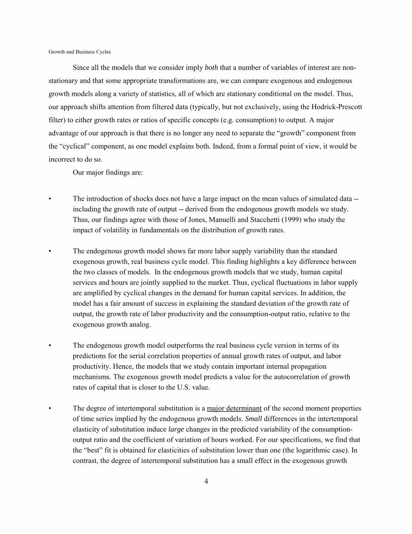
Our major findings are:

• The introduction of shocks does not have a large impact on the mean values of simulated data --including the growth rate of output -- derived from the endogenous growth models we study.Thus, our findings agree with those of Jones, Manuelli and Stacchetti (1999) who study theimpact of volatility in fundamentals on the distribution of growth rates.

• The endogenous growth model shows far more labor supply variability than the standardexogenous growth, real business cycle model. This finding highlights a key difference betweenthe two classes of models. In the endogenous growth models that we study, human capitalservices and hours are jointly supplied to the market. Thus, cyclical fluctuations in labor supplyare amplified by cyclical changes in the demand for human capital services. In addition, themodel has a fair amount of success in explaining the standard deviation of the growth rate ofoutput, the growth rate of labor productivity and the consumption-output ratio, relative to theexogenous growth analog.

• The endogenous growth model outperforms the real business cycle version in terms of itspredictions for the serial correlation properties of annual growth rates of output, and laborproductivity. Hence, the models that we study contain important internal propagationmechanisms. The exogenous growth model predicts a value for the autocorrelation of growthrates of capital that is closer to the U.S. value.

• The degree of intertemporal substitution is a major determinant of the second moment propertiesof time series implied by the endogenous growth models. Small differences in the intertemporalelasticity of substitution induce large changes in the predicted variability of the consumption-output ratio and the coefficient of variation of hours worked. For our specifications, we find thatthe “best” fit is obtained for elasticities of substitution lower than one (the logarithmic case). Incontrast, the degree of intertemporal substitution has a small effect in the exogenous growth


2 For analyses that emphasize cross country differences, see Mendoza (1997), Jones, Manuelli andStacchetti (1999), de Hek (1999), Fatas (2000).

5

model.

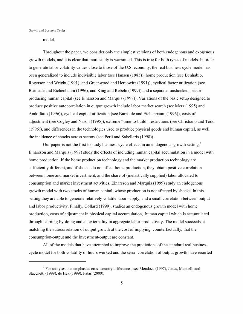
Throughout the paper, we consider only the simplest versions of both endogenous and exogenous

growth models, and it is clear that more study is warranted. This is true for both types of models. In order

to generate labor volatility values close to those of the U.S. economy, the real business cycle model has

been generalized to include indivisible labor (see Hansen (1985)), home production (see Benhabib,

Rogerson and Wright (1991), and Greenwood and Hercowitz (1991)), cyclical factor utilization (see

Burnside and Eichenbaum (1996), and King and Rebelo (1999)) and a separate, unshocked, sector

producing human capital (see Einarsson and Marquis (1998)). Variations of the basic setup designed to

produce positive autocorrelation in output growth include labor market search (see Merz (1995) and

Andolfatto (1996)), cyclical capital utilization (see Burnside and Eichenbaum (1996)), costs of

adjustment (see Cogley and Nason (1995)), extreme “time-to-build” restrictions (see Christiano and Todd

(1996)), and differences in the technologies used to produce physical goods and human capital, as well

the incidence of shocks across sectors (see Perli and Sakellaris (1998)).

Our paper is not the first to study business cycle effects in an endogenous growth setting.2

Einarsson and Marquis (1997) study the effects of including human capital accumulation in a model with

home production. If the home production technology and the market production technology are

sufficiently different, and if shocks do not affect home production, they obtain positive correlation

between home and market investment, and the share of (inelastically supplied) labor allocated to

consumption and market investment activities. Einarsson and Marquis (1999) study an endogenous

growth model with two stocks of human capital, whose production is not affected by shocks. In this

setting they are able to generate relatively volatile labor supply, and a small correlation between output

and labor productivity. Finally, Collard (1999), studies an endogenous growth model with home

production, costs of adjustment in physical capital accumulation, human capital which is accumulated

through learning-by-doing and an externality in aggregate labor productivity. The model succeeds at

matching the autocorrelation of output growth at the cost of implying, counterfactually, that the

consumption-output and the investment-output are constant.

All of the models that have attempted to improve the predictions of the standard real business

cycle model for both volatility of hours worked and the serial correlation of output growth have resorted


6

to various asymmetries. These include different production functions in the home, human capital, and

physical goods production sectors; in particular, they make strong assumptions about the capital-labor

ratio and differential elasticities of substitution across sectors that are not backed by evidence. In

addition, for the models to produce the desired results it is necessary to assume a particular pattern of

incidence for the technology shocks: in most models, the human capital (or the home production) sector

is not subject to any shocks, since this facilitates substitution in and out of market work, increasing the

volatility of measured hours. Finally, several of the models resort to (difficult to measure) adjustment

costs.

Our model contributes to this literature by showing that realistic values of labor supply volatility,

autocorrelation in output growth, and a number of other second moments, can be attained without

resorting to asymmetries -- in either production technologies or the incidence of productivity shocks --

and costs of adjustment. Unlike the papers described above, we put emphasis on the role of the

intertemporal elasticity of substitution, and on matching model and historical data that are rendered

stationary in a manner consistent with the theory.

In section 2, we begin by laying out a general formulation of the class of models that we are

interested in studying and provide a simple methodological tool for handling the fact that the natural state

space is unbounded. In section 3, we take an initial look at the quantitative properties of a simple class of

these models with equal depreciation rates for physical and human capital. In section 4, we consider

alternative versions of the model with different depreciation rates for the two capital goods and allow for

the possibility that investment in human capital is partly omitted from the income and product accounts

altogether. Finally, section 5 provides some concluding comments.

2. A General Model

The class of models that we are interested in studying feature investment in both human and physical

capital and a time stationary technology that is subjected to random shocks. They are stochastic versions

of the convex models described in Jones and Manuelli (1990). A general specification that captures these

features is given by:

(2.1) Max E{Pt βt u(ct,ot) }subject to,


7

ct + xzt + xht + xkt @ F(kt,zt,st)zt @ M(nzt,ht,xzt)kt+1 @ (1-δk) kt + xkt

ht+1 @ (1-δh) ht +G(nht,ht,xht)ot + nht +nzt @ 1,h0 and k0 given.

Here {st} is a stochastic process which we assume is Markov with a time stationary transition

probability function, ct is consumption, xkt is investment in physical capital, kt is the stock of physical

capital, xht is investment in human capital, ht is stock of human capital, zt is “effective labor,” nzt is hours

spent in the market working, nht is hours spent in augmenting human capital and ot is leisure. The

depreciation rates on physical and human capital are given by δk and δh, respectively. If F, M and G are

concave and bounded below by a homogenous of degree one function, it is possible to show that the

competitive equilibrium allocation coincides with the solution to the planner's problem and, for some

parameter values, displays income (and consumption) growth.

Thus, this is a fairly standard endogenous growth model in which effective labor is made up of a

combination of hours and human capital which is supplied to the market. For specific choices of

functional forms, many models in this literature are special cases of this formulation. For example, if M =

nzh and G = G0hnh, the model corresponds to that of Lucas (1988) in the absence of externalities. If M =

nzh and G = xh, this corresponds to the two capital goods version discussed in Jones, Manuelli and Rossi

(1993).

The actual solution of models in this class does cause some problems, however. The natural

choice of the state is the vector (kt,ht,st). The problem that this poses is that both kt and ht are diverging to

infinity (at least for versions of the model that exhibit growth on average). To solve this problem, the key

property that we exploit is that for models of this type to have a balanced growth path, both preferences

and technology must be restricted in a specific way (see King, Plosser and Rebelo (1988), and Alvarez

and Stokey (1998)). For our numerical strategy, it suffices that the model satisfies:

Assumption: Preferences and Technology

a) The instantaneous utility function satisfies,

W v(o) c1-σ/(1-σ) with σ£ 1, but σ > 0, oru(c,o ) = X

Y log(c) + v (o) with σ = 1b) F is concave and homogeneous of degree one in (k,z)


8

c) M is concave and homogeneous of degree one in (h,xz)

d) G is concave and homogeneous of degree one in (h,xh).

These restrictions, in turn, imply that knowledge of the current shock and the current human

capital to physical capital ratio (the two relevant pseudo state variables) is sufficient to determine the

optimal choices of employment and next period's human to physical capital ratio. Given the state, the

current stocks, the productivity shock and the current level of employment it is possible to determine

consumption and future capital stocks using static first order conditions.

Indeed, the property that there is a transformation of the problem in which all the (relevant)

variables are stationary is a special case of a much more general (and fairly standard) argument. Our

assumptions about the technological side of the model imply that holding the vector of labor supplies

fixed, a time path of the endogenous variables, zt (interpreted as the entire state/date contingent plan) is

feasible from initial state (h0, k0, s0) if and only if λzt is feasible from the initial state (λh0, λk0, s0) (λ > 0).

That is, the feasible set is linearly homogeneous holding the vector of labor supplies fixed. Moreover,

utility also has a homogeneity property -- again holding labor supplies fixed, the utility (i.e., the entire

expected discounted sum) realized from λzt is λ1-σ times the utility of zt (at the same labor supplies).

Formally, consider the maximization problem:

(2.2) Max U(z, n)

subject to

(z,n) M Γ(h0, k0, s0),

where, as noted, (z, n) is interpreted as the entire date/state contingent path of the endogenous variables

and vector of labor supplies and U is the resulting expected discounted sum of utilities. Let V(h0, k0, s0)

denote the maximized value in this problem (assuming that it exists) and let (z*(h0, k0, s0), n*(h0, k0, s0))

denote the optimal plan.

Proposition 1: Assume that the utility function in (2.2) is homogeneous of degree 1-σ in z (holding n

fixed) and that the feasible set, Γ, is linearly homogeneous in (h, k) (holding n and s fixed) and that a

solution exists for all (h, k, s). Then, the value function, V, for the problem (P.2) satisfies V(λk, λh, s) =


3 This is obviously an extreme assumption. However, we were unable to obtain estimates of the physicalcapital - labor or physical capital - human capital ratios in specific activities like education and health.

9

λ(1-σ) V(k,h,s), for all λ>0. Moreover, the optimal choice of z is homogeneous of degree one and the

optimal choice of n is homogeneous of degree zero -- (z*(λk, λh, s), n*(λk, λh, s)) = (λz*(h, k, s), n*(h ,k

,s)).

Proof: See Appendix A.

3. A Simple Example with Endogenous Growth and Equal Depreciation

In this section, we study the properties of a calibrated version of the model. Our objective is twofold:

First, we want to understand how intertemporal substitution affects the implications of the model;

second, our intent is to compare this class of endogenous growth models with a more standard real

business cycle model (with constant, exogenous growth). To this end, we not only parameterize a version

of the model of section 2, but we also analyze a “related” exogenous growth model similar to those

studied in the real business cycle literature.

3.1 Calibrating the Model

To specialize the model of section 2, we adopt the restrictions on preferences outlined above, and assume

that the production function is given by F(k, nh, s) = sAkα(nh)1-α. The laws of motion for physical and

human capital are: k' = (1-δk) k + xk and h' = (1-δh) h + xh. We also assume that both capital stocks

depreciate at the same rate, that is, δk = δh. From a formal point of view, our choice of a linear law of

motion for capital amounts to an aggregation assumption: the technology used to produce investment in

human capital goods (education, training, and health among others) is identical to the technology used to

produce general output.3

Using the two stochastic Euler equations of the model, it follows that,

Et [uc(t+1)(αF(t+1)/kt+1 - (1- α)F(t+1)/ht+1)]= 0.


10

Hence, in any interior equilibrium, ht/kt = (1-α)/α for all t. This is an important property of the

specification of a Cobb-Douglas production function with equal depreciation rates: the human to physical

capital ratio is independent of the level of employment and the productivity shock. Given this, and

defining A* L A(1-α)1-ααα, it follows that

(3.1) ct = kt [stA* nt1-α ((1-nt)/nt) ((1-α)/αψ)] L kt g1(st,nt).

Using this, we obtain,

(3.2) .kt�1�kt st A � n 1�αt 1� 1�α

ψ1�nt

nt

�1�δ L ktg2(st,nt)

Finally, after substitution, the relevant Euler equation becomes:

(3.3) [g1(st,nt) (1-nt)ψ]-σ (1-nt)ψ = β fS{[g2(st,nt)g1(st+1,nt+1)(1-nt+1)ψ]-σ

×(1-nt+1)ψ[1-δ+st+1A*(nt+1)1-α]P(st,dst+1)}.

A solution to this equation is a function n*:S S [0,1] with nt=n*(st). Note that given n*, the

solution to the planner's problem (and the competitive equilibrium for this economy) can be completely

described using (3.1) and (3.2) and ht+1 = kt+1(1-α)/α.

Our model puts restrictions on concepts that -- although clearly identifiable from a theoretical

point of view -- are difficult to measure. Prime examples are consumption and investment in human

capital. In the data, private expenditures on schooling and health (arguably investments in human capital)

are assumed to be part of consumption, and some forms of investment (e.g. training) are likely to remain

unmeasured. In the model, those expenditures are more properly viewed as being investments in human

capital. The resolution of this problem is not easy. As a first approximation, and we change this in

section 4, we assume in our calibration that measured consumption (in the National Income and Product

Accounts) corresponds to the sum of consumption and investment in human capital in the model, c + xh.

Thus, it is the variable that enters the utility function, along with the level of investment (or spending) in

human capital that coincides with measured consumption.

We set capital's share, α, equal to 0.36, and hold β fixed at 0.95. We set δk = δh = 0.075. This is a


4 Since our non-stochastic model has the balanced growth property, our procedure forces the shock toexplain the productivity slowdown that started in the mid-seventies. This implies that, in our sample, the estimatedshocks are decreasing from a peak of 1.07 (7% above average) in 1966. Even though feasible, modeling theproductivity slowdown is beyond the scope of this paper. For alternative explanations see Greenwood andYorukoglu (1997), Caselli (1999) and Manuelli (2000).

5 The difference in the estimated standard deviation here relative to the endogenous growth specification isdue to the fact that the former allows the growth rate to covary with the shock, while the latter fixes it a 1.38%.

11

compromise between the relatively high values for physical investment used in the literature and the

small values typically estimated for depreciation of human capital. We relax this assumption in section 4.

Finally, we choose the remainder of the parameters of the model so as to match the average growth rate

of U.S. output over the 1955-1992 period of 1.38% per year and average labor supply equal to 0.17 (see

Jones, Manuelli and Rossi, (1993)). These two facts (γ = 1.38% and n = 0.17) pin down two of the three

remaining parameters of the model, σ, ψ, and A. This leaves one degree of freedom in the choice of

these parameters. Since one of our interests is to determine how the degree of intertemporal substitution

affects the business cycle properties of the model, we vary σ from 0.9 to 3.0 while simultaneously

changing A and ψ so that along the model's non-stochastic balanced growth path, γ = 1.38% and n = 0.17.

We assume that the process, st, is given by st = exp[zt - σ2ε/2(1-ρ2)] with zt = ρzt + εt+1, where the ε's

are i.i.d., normal with mean zero and variance σ2ε. It follows that E(st)=1. To choose ρ and σ2

ε, we use the

fact that, with δk = δh, the ratio ht/kt is identically (1-α)/α, and hence, output is given by yt = A st ( (1-

α)/α)1-α kt (nt)1-α. Thus, given data on output, the capital stock and hours, the time series of st can be

directly identified up to the constant A ((1-α)/α)1-α. We use the data set from Burnside and Eichenbaum

(1996) (renormalized to reflect annual frequencies) to construct the implied time series of st given α.

Using this series -- which is not obviously the realization of a stationary process -- we estimate ρ and σ2ε

to be 0.95 and 0.0146, respectively.4 Table A.1 in Appendix A shows all the combinations of parameters.

The model that we study has a “related” exogenous growth version. More precisely, if ht -- our

human capital variable -- is assumed to grow exogenously at the rate γU , the technology becomes F(k, nh

,s) = sAtkα(n)1-α, with At = A(ht)1-α = AU γU t. Given this specification, st is calculated using the same

procedure as before. In this case, the estimated parameters are ρ = 0.95 and σ2ε = 0.0126.5

To solve the model we use the method of parameterized value function iteration as discussed in

Siu (1998). The method finds a linear combination of Chebychev polynomials to approximate the value

function in the recursive representation of the model. This is done by iterating upon the contraction

mapping over a discretization of the state space until the fixed point is found. See Appendix B for details.


6 This is a product of our simplifying assumptions. Given our calibrated value for the depreciation rate, theshare of output needed to maintain human capital along the balanced growth path is large, and the share needed tomaintain physical capital is small (and incompatible with investment’s share in the data). See section 4 for versionsof the model in which both of these assumptions are relaxed.

7 We report only the standard deviation of the investment-output ratio since, in the model, y = c + xh + xk,and it follows that σ(xk/y) = σ ((c+xh)/y). Hence, by construction, the variability of the consumption-output ratio andthe investment-output ratio coincide.

12

We used simulations of time series of the endogenous variables of the models with T=5000 periods in

order to calculate estimates of key population moments. To facilitate comparisons, throughout the paper,

the same realization of {st} was used for all cases with the same parameters for the stochastic process.

3.2 Some Results

As indicated above, our purpose is to assess the performance of the model in terms of its ability to

replicate the distribution of observed variables, and to study the differences in propagation mechanisms

between the endogenous and the exogenous growth models. We concentrate on four dimensions of that

distribution: mean, standard deviation, autocorrelation and cross correlations.

In previous work, Jones, Manuelli and Stacchetti (1999) find that the introduction of technology

shocks in a class of endogenous growth models does not have a large effect on the mean values of the

endogenous variables, relative to their (non-stochastic) balanced growth values, unless the shock variance

is fairly large. We find the same pattern for the specifications in this paper: the introduction of

uncertainty results in slightly higher simulated mean growth rates, but quantitatively the effect is small.

Moreover, the results are only slightly affected by the magnitude of the intertemporal elasticity of

substitution. The average value of growth rates in the exogenous growth model are virtually identical to

their balanced growth values, irrespective of the value of σ. However, the average value of labor supply

does differ from its calibrated value, particularly when intertemporal substitution is low. In the

endogenous growth version the share of physical capital investment in output, when we “allocate” all of

the investment in human capital to consumption, is slightly lower than in the data, and the share of “true”

consumption in output is low.6 The results are displayed in Table A.2 in Appendix A.

Table 3.1 presents the results for the standard deviation of the growth rates of output, γ, and labor

productivity, γy/n, the investment-output ratio, xk/y,7 and the coefficient of variation in hours worked, n;

this is done for both the endogenous growth model and its exogenous growth counterpart. In the context


8 This may explain why this literature has typically not explored the effects of alternative values of theelasticity of substitution. For a good survey see Cooley (1995).

13

of the models that we study all of these variables are stationary. The final row of the table gives the

corresponding values for the U.S. from the Burnside and Eichenbaum (1996) data.

Table 3.1: Volatility - Endogenous Growth and Real Business Cycle Models

Case σ σ(γ) σ(γ) - R σ(xk/y) σ(xk/y)-R σ(n)/n�� σ(n)/n�� -R σ(γy/n ) σ(γy/n )-R

1 0.90 .0371 .0182 .0163 .0116 .1008 .0124 .0161 .0100

2 1.00 .0286 .0175 .0102 .0106 .0622 .0113 .0130 .0103

3 1.25 .0216 .0165 .0051 .0090 .0301 .0096 .0130 .0108

4 1.50 .0191 .0159 .0033 .0082 .0187 .0086 .0136 .0111

5 1.75 .0178 .0156 .0023 .0077 .0128 .0081 .0140 .0113

6 2.00 .0171 .0153 .0017 .0074 .0093 .0077 .0142 .0114

7 2.50 .0162 .0150 .0010 .0071 .0052 .0073 .0146 .0116

8 3.00 .0157 .0147 .0006 .0070 .0029 .0071 .0148 .0117

U.S. .0214 .0214 .0119 .0119 .0342 .0342 .0124 .0124Note: The column labeled σ(z) gives the standard deviation of z, where z corresponds to the growth rate of output(γ), the investment/output ratio (xk/y), the growth rate of labor productivity (γy/n), and labor (n). The term n� denotesmean number of hours. An R indicates that the column corresponds to the values of a “real business cycle” versionwith exogenous growth as described in the text.

The first important observation is that, unlike its impact on the first moments of the distribution,

changes in the intertemporal elasticity of substitution (1/σ) have a large impact on the second moments of

most variables of the endogenous growth model. In stark contrast, it has a relatively small impact in the

exogenous growth model.8 For example, increasing σ from 0.9 to 3.00 decreases the variability in hours

worked by a factor of 35 in the endogenous growth model; in the exogenous growth model this

experiment decreases the same variability by a factor of 1.75.

The endogenous growth model does quite well at moderate values of σ. For example, when σ =

1.25, the standard deviation of output growth from the model is virtually identical to that in the data, the

standard deviation of the investment-output ratio is 43% of the U.S. value, the coefficient of variation of

hours worked is 88% of the estimated U.S. value, and the standard deviation of the growth rate of labor


9 This is true irrespective of the calibrated non-stochastic balanced growth value of labor supply, andhence, the calibrated value of ψ. In experiments, we have calibrated the model using n = 0.3, a value close to thoseused in the real business cycle literature. None of the substantive results presented in this paper are sensitive to thischoice.

14

productivity exceeds the U. S. value by 5%. Except for the standard deviation of the investment-output

ratio (or, equivalently, the consumption-output ratio) the endogenous growth model studied here

performs better than its exogenous growth counterpart. This is particularly evident in the volatility of the

growth rates and hours worked.9 In the next section, we show how natural extensions of the endogenous

growth model improve its ability to match the volatility in the measured consumption- and investment-

output ratio.

Table 3.2 reports the autocorrelation properties of the endogenous variables from the simulation,

for both the endogenous growth model and its exogenous growth counterpart.

Table 3.2: Autocorrelations - Endogenous Growth and Real Business Cycle Models

Case σ ρ1(γy) ρ1(γy)- R ρ1(γc+xh) ρ1(γc)- R ρ1(n) ρ1(n)- R ρ1(γy/n) ρ1(γy/n)- R

1 0.90 .169 -.019 .247 .316 .949 .744 .972 .201

2 1.00 .145 -.014 .199 .239 .949 .767 .763 .156

3 1.25 .114 -.007 .141 .146 .949 .805 .344 .101

4 1.50 .098 -.004 .115 .104 .949 .830 .211 .074

5 1.75 .089 -.003 .100 .081 .949 .849 .154 .059

6 2.00 .082 -.002 .090 .066 .949 .864 .124 .049

7 2.50 .073 -.001 .077 .049 .949 .888 .093 .037

8 3.00 .067 -.000 .069 .038 .949 .906 .077 .029

U.S. .213 .213 .400 .400 .825 .825 .295 .295Note: The column labeled ρ1(z) corresponds to the first order autocorrelation coefficient of z, where z correspondsto the growth rate of output (γy), consumption (c+xh), labor productivity (γy/n), and the level of the number of hoursworked (n). An R indicates that this corresponds to the output of a “real business cycle” version with exogenousgrowth as described in the text.

There are several interesting results. First, the endogenous growth model generates persistence in

output growth for all values of σ considered; the degree of first order autocorrelation increases with the

intertemporal elasticity of substitution. Quantitatively, the endogenous growth model with equal

depreciation rates can account for about 50% of the degree of persistence in growth rates for values of σ


15

near one. In the exogenous growth model, in all cases, the autocorrelation of output growth is negative.

This, of course, is just another instance of the well known failure of real business cycle models to display

realistic propagation mechanisms (see Cogley and Nason (1995)).

Second, both models explain a relatively small amount of the observed autocorrelation of the

growth rate of consumption. If anything, the exogenous growth model performs better for high values of

the intertemporal elasticity of substitution. Third, in the endogenous growth model, the autocorrelation of

hours worked coincides with that of the shock and, for our specification, overstates the measured

autocorrelation by 15%. The exogenous growth model does better in this dimension and, for some

specifications, almost perfectly matches the data. Fourth, the endogenous growth model is able to match

the autocorrelation in the growth rate of labor productivity for a value of σ between 1.25 and 1.50, while

the real business cycle model understates it for all cases considered.

Finally, for both specifications -- endogenous and exogenous growth -- the autocorrelation of

growth rates of the endogenous variables depends on the intertemporal elasticity of substitution. Using

the autocorrelation as the target dimension, the endogenous growth model still “prefers” a risk aversion

coefficient of σ = 1.25, while the exogenous growth version “prefers” σ = 0.90. The latter, however, does

a poor job matching the autocorrelation of the growth rate of output at all values of σ.

The last statistic we present are the cross correlations --at several leads and lags-- of the growth

rates of output and labor productivity, and the levels of hours worked and the investment-output ratio,

with the growth rate of output. Since it is cumbersome to report all the results for the different values of

intertemporal substitution, we choose the values of σ that better match the data for both models. Again,

this criterion “selects” σ = 1.25 for the endogenous growth version, and σ = 0.9 for the exogenous growth

version. Table 3.3 contains the estimates of the cross correlations generated by both models, as well as

the corresponding statistics from the U.S.


16

Table 3.3: Cross Correlations with Output Growth - Endogenous Growth(bold), Exogenous Growth, and U.S. Data (italics).

(Endogenous σ = 1.25 - Exogenous σ = 0.9)

Lag (j) -2 -1 0 1 2

γy,t+j 0.100-0.012-0.081

0.114-0.0190.214

1.0001.0001.000

0.114-0.0190.214

0.100-0.012-0.081

nt+j 0.196-0.053-0.328

0.209-0.057-0.327

0.5070.6240.118

0.4840.4710.308

0.4590.3580.280

γy/n,t+j 0.143-0.0220.272

0.158-0.0290.384

0.9620.9610.482

0.2450.158-0.166

0.2260.1210.144

(xk/y)t+j 0.195-0.052-0.315

0.209-0.057-0.139

0.5060.6240.509

0.4830.4700.454

0.4580.3570.159

Overall, neither model is a complete successes at matching the cross-correlation structure of the

data. As indicated above, the endogenous growth model generates more persistence, and this appears in

the form of higher autocorrelation values for the growth rate of output. It also captures the pattern of

cross-correlations between productivity and output growth. The exogenous growth model does a better

job of matching the cross-correlation between hours and growth rates.

For the sake of comparison with the real business cycle literature we followed the standard

practice of taking logs and Hodrick-Prescott filtering the data. We then calculated the standard deviation

of all relevant variables -- the analog of Table 3.1 -- for all cases, as well as the cross correlation of

detrended output, hours, labor productivity and investment with output at different leads and lags for the

“best” cases -- the analog of Table 3.3; the results are in Tables A.3 and A.4 in the appendix. Overall, the

general flavor of the simulated results is similar to those found using the stationary ratios: The

endogenous growth model predicts that small differences in the degree of intertemporal substitution

result in substantial differences in the standard deviation of most variables. In addition, it outperforms the

real business cycle model in terms of predicting standard deviations for all variables that are closer to

observed U.S. values. In terms of cross-correlations, both models are fairly successful at matching the

autocorrelation of detrended output. As in the case of unfiltered data, both models feature high

contemporaneous correlations among the variables, and these estimates are too high relative to the U.S.

data. For both models, hours lead the cycle much more than in the data while labor productivity lags the


17

cycle more than in the data. Overall, the endogenous growth and the exogenous growth versions are

fairly comparable using Hodrick-Prescott filtered data according to these measures.

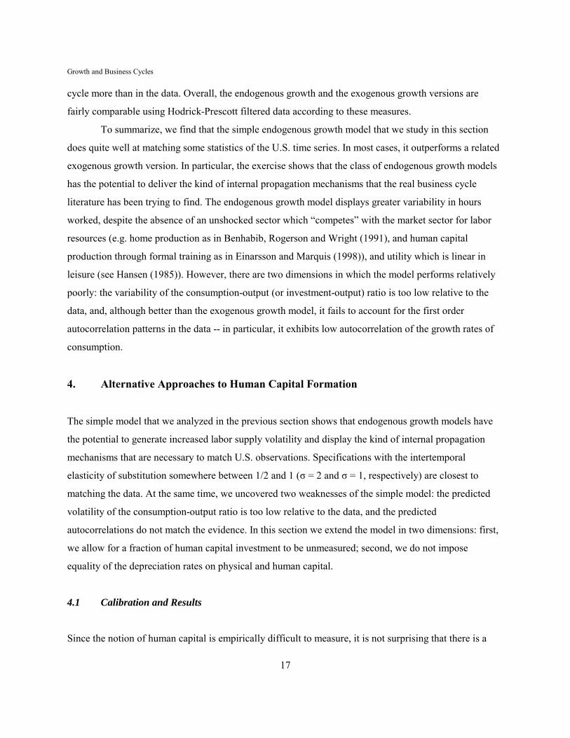
To summarize, we find that the simple endogenous growth model that we study in this section

does quite well at matching some statistics of the U.S. time series. In most cases, it outperforms a related

exogenous growth version. In particular, the exercise shows that the class of endogenous growth models

has the potential to deliver the kind of internal propagation mechanisms that the real business cycle

literature has been trying to find. The endogenous growth model displays greater variability in hours

worked, despite the absence of an unshocked sector which “competes” with the market sector for labor

resources (e.g. home production as in Benhabib, Rogerson and Wright (1991), and human capital

production through formal training as in Einarsson and Marquis (1998)), and utility which is linear in

leisure (see Hansen (1985)). However, there are two dimensions in which the model performs relatively

poorly: the variability of the consumption-output (or investment-output) ratio is too low relative to the

data, and, although better than the exogenous growth model, it fails to account for the first order

autocorrelation patterns in the data -- in particular, it exhibits low autocorrelation of the growth rates of

consumption.

4. Alternative Approaches to Human Capital Formation

The simple model that we analyzed in the previous section shows that endogenous growth models have

the potential to generate increased labor supply volatility and display the kind of internal propagation

mechanisms that are necessary to match U.S. observations. Specifications with the intertemporal

elasticity of substitution somewhere between 1/2 and 1 (σ = 2 and σ = 1, respectively) are closest to

matching the data. At the same time, we uncovered two weaknesses of the simple model: the predicted

volatility of the consumption-output ratio is too low relative to the data, and the predicted

autocorrelations do not match the evidence. In this section we extend the model in two dimensions: first,

we allow for a fraction of human capital investment to be unmeasured; second, we do not impose

equality of the depreciation rates on physical and human capital.

4.1 Calibration and Results

Since the notion of human capital is empirically difficult to measure, it is not surprising that there is a


10 From the “income” side, training that is paid for by firms, i.e. not deducted from wages, appears asdecreased profits in the period in which those investments are made. A very good discussion that illustrates the keyissues appears in Howitt (1997).

18

paucity of estimates of the depreciation rate, δh. Haley (1976) estimates δh to be somewhere between 1%

and 4%. Heckman (1976) obtains point estimates that are similar to Haley's, but are not significantly

different from zero. Earlier work by Ben-Porath (1967) estimates δh close to 9%. The results in Jorgenson

and Fraumeni (1989) are consistent with depreciation rates that range between 1% and 3%. In order to

cover the range of estimates, we experimented with three values of δh: a low value of 0.01, an

intermediate value of 0.04, and a high value of 0.07.

The second issue that we have to deal with is what part of investment in human capital is

included in measured GNP. There are several categories of investment in human capital that are likely to

be omitted from standard GNP accounting. The single largest category is on-the-job-training and on-the-

job-learning. In both cases, it is possible that a fraction of these costs is not counted in standard measures

of output.10 In addition, acquisition of human capital at home (e.g., time of both children and parents),

and student inputs at school are not measured. A second difficulty is that, as indicated above, whatever is

measured is scattered between government spending and private consumption. As in section 3, we solve

this problem by allocating the measured component of investment in human capital to measured

consumption. It is difficult to estimate what fraction of “true” investment in human capital is included in

GNP. Considering only training (which is likely to be excluded) its contribution has been estimated

somewhere between 50% of total investment (Mincer (1962)) to just over 20% (Heckman, Lochner and

Taber (1998)). Our approach is to assume that only a certain fraction, η, of investment in human capital

is included in GNP. We vary the possible values of η from a low of 0.25 to a high of 1.0.

Since there is (potentially) an unmeasured component of output, measured GNP will differ from

“true” output. In particular, measured GNP is c + xk + ηxh. Since we continue to assume that all of the

model’s labor input is accounted for in the data, we interpret the unmeasured part of xh as on-the-job-

training that workers receive while employed. This interpretation requires recalibrating the model. To see

this, note that if we continue to denote labor's share of GNP by (1-α), then it must be that case that (1-α)

GNP = w (nh) + (1-η) xh. This implies lower values of α than are commonly used in the literature. From

now on, we will use the term GNP to refer to measured output, and use simply output to denote the total

amount of goods and services produced.


11 The table includes a 37th case that will be discussed later.

12 Formally the identification assumption that allowed us to estimate the shock, δh= δk, does not hold anylonger. However, the estimation in the exogenous growth version yielded a very similar process for st. Moreover, weexperimented using an actual series for ht from the work of Kendrick (1976), Eisner (1989), and Jorgensen andFraumeni (1989) and, in each case, we obtained ranges for ρ and σε that include those used in section 2. Given thelarge amount of uncertainty associated with these estimates, we did not see any compelling reason to change theestimates used in section 3.

19

As in the previous section, we set β = 0.95, and choose the remainder of the parameters to match

long run U.S. observations. These include the average growth rate of output of 1.38% and average labor

supply equal to 0.17. In addition, we require payments to capital to be 36% of measured output, and

physical capital investment’s share of measured output to be 24.4%. This leaves three degrees of freedom

in the choice of parameters. We experiment with different values of σ, δh and η to see how the model

differs from those in section 3. Note that in performing these adjustments, the calibrated values of α, A,

δk and ψ respond to maintain our identifying assumptions. For our numerical exercise we considered the

following configurations:

σ ε {1.00, 1.25. 1.50, 2.00}, η ε {0.25, 0.50, 1.00}, and δh ε {0.01, 0.04, 0.07}

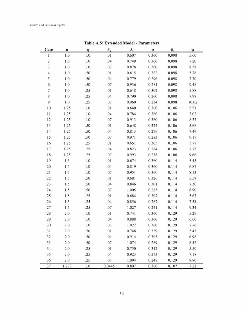
In all, we computed 36 different cases. A complete description of the parameters is in Table A.5.11

For the stochastic shock process, we used the same parameters as in the previous section.

(Indeed, we used the same realization for the simulations.) This allows us to do direct comparisons of the

results with those of the previous section.12 Finally, since there is no “obvious” exogenous growth analog

of the model in this section, we continue using the results from section 3 for the purposes of comparison.

As in section 3, the model's implications for the means of the variables of interest result in small

deviations from their calibrated values, and we do not report the results here. The implications of the

model for the standard deviations of the growth rates of GNP, γ, and labor productivity, γy/n, the ratio of

measured consumption to GNP, (c + ηxh)/GNP, and the coefficient of variation of hours worked, σ(n)/nO,

are in Table A.6. There are several results of interest:

• The volatility levels for the growth rate of GNP, the share of measured consumption in GNP,hours and labor productivity can be matched simultaneously with reasonable values of σ, δh andη. One set of parameters that works fairly well is σ = 1.25, δh = .04 and η = 1.0. We discuss acase similar to this one in detail below.


20

• In almost all cases, logarithmic utility generates volatility levels for all of the variables that arehigher than in the data, while they are typically too low when σ = 2.0. Again, this is in contrast tothe exogenous growth model, where these volatilities are uniformly too low.

• For the most part, all standard deviations decrease in δh. The magnitude of this decrease is quitesensitive to the size of the depreciation rate of human capital.

• The effects of η -- the share of “true” investment in human capital that is measured in GNP -- aresmall for all variables except for the growth rate of labor productivity, γy/n. For this variable, themodel predicts too much variability unless all of xh is measured (η = 1).

Thus, one lesson learned from these experiments is that the model's predictions for the standard

deviations of the endogenous variables are quite sensitive to the choice of parameters. We experimented

with our choices of (σ, η, δh) seeking to match the values of σ(γ), σ[(c+ηxh)/GNP] and σ(n)/nO, found in

the U.S. data. The results, along with those of the “best” exogenous growth model from section 3, are in

Table 4.1.

Table 4.1: Extended Model - Volatility

Case σ, η, δh σ(γ) σ[(c+ηxh)/GNP] σ[xk/GNP] σ(n)/n�� σ(γy/n)

37 1.273, 1.0, 0.0445 0.0219 0.0118 0.0118 0.0341 0.0126

RBC 0.90, 1.0, 0.075 0.0182 0.0116 0.0116 0.0124 0.0100

U.S. 0.0214 0.0119 0.0119 0.0342 0.0124

For our preferred case -- case 37 -- the match between model and data is almost perfect. The

estimates are, at most, within 2% of the observed valuesOn the other hand, the exogenous growth version

falls moderately short in the standard deviations of the growth rates of GNP and labor productivity (about

80% of the U.S. values), and only reproduces approximately 1/3 of the U.S. coefficient of variation for

hours worked.

Why is it that relaxing the assumption of equal depreciation rates generates such a big difference

in the volatility of measured consumption? The reason is simple: If δh is smaller than δk the balanced

growth value of h/k increases. This has two effects: on the one hand, a higher value of the stock of human

capital requires more investment in it. On the other hand, the lower depreciation rate implies that less

investment is required. In the examples we have looked at, the second effect dominates. This is important


13 We also varied the share of human capital investment included in measured GNP, η. Our preferredspecification has η equal to one. Moreover, the volatility of the measured consumption-output ratio is fairlyinsensitive to η and, hence, we do not discuss the effects of changing this parameter.

21

because our definition of measured consumption is c + ηxh, and it was the divergent behavior of the two

components that resulted in the low estimates of its variability in section 3.13

In section 3 we pointed out that the model failed to account for the autocorrelation of

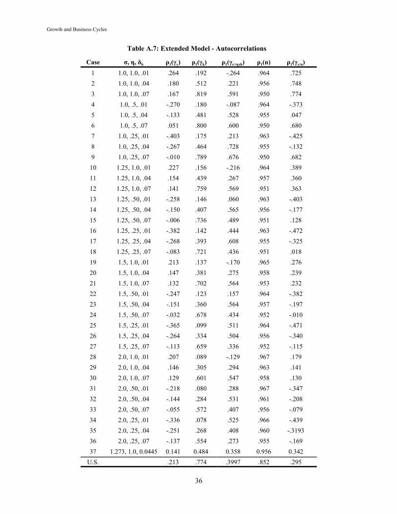
consumption growth. The extended model is a substantial improvement. Table A.7 in the appendix

contains the results for all 37 cases. There are a few interesting regularities:

• If human capital depreciation is small and the share of measured human capital investment isclose to one, it is relatively easy for the model to produce persistence in output growthresembling values found in the U.S. data (around 0.2). The first order autocorrelation of outputgrowth is decreasing in δh when η = 1, whereas it is increasing in δh when η = 0.5 and 0.25.Hence, the autocorrelation of output growth seems to be more sensitive to η than to δh.

• On the other hand, the autocorrelation of measured consumption growth is extremely sensitive tothe value of δh. In fact, when δh equals 0.01 the model produces negative autocorrelation.

As before, we find it encouraging that small variations in the parameters result in relatively large

changes in the predicted values. It is of interest to evaluate how well our preferred specification -- chosen

to match three measures of volatility in the data -- does in terms of accounting for the autocorrelation of

endogenous variables. The results, along with those for the exogenous growth model, are reported in

Table 4.2.

Table 4.2: Extended Model - Autocorrelations

Case σ, η, δh ρ1(γy) ρ1(γk) ρ1(γc+ηxh) ρ1(n) ρ1(γy/n)

37 1.273, 1.0, 0.0445 0.148 0.484 0.358 0.956 0.342

RBC 0.9, 1.0, 0.075 -0.019 0.740 0.316 0.744 0.201

U.S. 0.213 0.774 0.400 0.852 0.295

Even though the fit is not perfect, our endogenous growth model displays distinct propagation


14The intuition behind these cross correlation results becomes apparent when we consider theimpulse response behavior of the model. This is done in the next subsection.

22

mechanisms. It accounts for 70% of the first order serial correlation in the annual growth rate of output,

and it overestimates the first order serial correlation of productivity growth by approximately 15%. The

autocorrelations of consumption growth and hours worked are within 10% of the U.S. values. The one

significant deviation is the autocorrelation in the growth rate of capital: the endogenous growth model's

prediction is close to half the U.S. value, while the exogenous growth model implies a much closer fit.

Using the first order autocorrelation as a metric, the endogenous growth model outperforms its

exogenous growth counterpart if the growth rate of capital is ignored. Again, the important difference lies

in the two models' abilities to account for the first order serial correlation properties of the growth rate of

output. The exogenous growth model predicts a negative value, while the endogenous growth version

predicts a significantly positive autocorrelation.

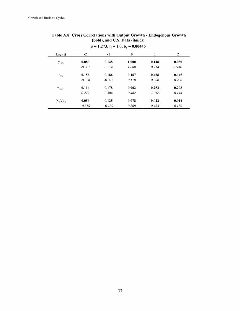
Finally, we computed the cross correlations with GNP growth for our preferred specification.

The results are reported in Table A.8, and show no substantial improvement over our findings in section

3. The model still generates an excessively high contemporaneous correlation between GNP growth and

labor productivity. Moreover, the contemporaneous correlation between output growth and the physical

capital investment-output ratio represents a distinct deterioration over the equal depreciation rate version

analyzed in section 3. Hours worked now lags the cycle, as it does in the data, though this correlation

pattern is marginal at best.14

4.2 The Dynamics of a Response to Shock

To understand how the extended model improves the serial correlation properties of measured

consumption, it is necessary to explore how a shock affects investment in both physical and human

capital. For the class of models in which δh < δk, a positive technology shock results not only in an

increase in investment in physical capital, xk, but also in an increase in xk relative to xh.

To understand the effects involved assume that, initially, the economy is operating along its

balanced growth path with st = 1. From the Euler equation it follows that,


15 Of course the explanation is only approximate since the theory only restricts the integral, and not eachterm, to be zero. However, it captures the right effects. In addition, the reader can check that our arguments gothrough for any homogeneous of degree one function, and not just the Cobb-Douglas case.

23

F(t)/ht(αht/kt - (1-α)) = δk - δh > 0.

Next, the no arbitrage condition is just,

Et[uc(t+1) (δh - δk + st+1F(t+1)/ht+1)(αht+1/kt+1 - (1-α))] = 0,

where, following a positive shock to st, st+1 is likely to be greater than one. If the solution kept ht+1/kt+1 =

ht/kt, then it follows that (δh - δk + st+1F(t+1)/ht+1)(αht+1/kt+1 - (1-α)) would be positive, violating the no-

arbitrage condition. Thus, the optimal policy is such that ht+1/kt+1 < ht/kt, and this, in turn, results in

relatively low investment in human capital in the period of a positive shock.15 One interpretation for this

is that in good times there is a (relative) increase in physical capital investment and a (relative) decrease

in human capital investment, while individuals increase their participation in the labor market. It is

important to note that this is not driven by competing uses of time. In our extended model, physical and

human capital are produced using the same technology and, hence, are subject to the same stochastic

shock. The true reason lies in the durability of the two forms of capital: since human capital depreciates

slowly, it is optimal to postpone investing in it until the technology shock is lower. In terms of our

aggregate model, one interpretation of this result is not only that individuals invest less in human capital,

but also that firms postpone training in good times, even though they go ahead with other investment

plans. This is consistent with anecdotal evidence.

In this model, “measured” consumption is c + ηxh. Thus, the response of measured consumption

to a shock is the sum of two individual effects, “pure” c and “pure” xh, that, to some extent, reinforce

each other, instead of moving in opposite directions, as in the case where δk = δh. It follows that both

“permanent income” and “equality of rate of return” type of arguments work in the same direction and

result in long lasting impacts on measured consumption as a result of a technology shock.

In Figure 1, we show the response of the two forms of investment to a positive one standard

deviation shock to productivity. The values are computed from our preferred specification (case 37

above) and are such that the shock “hits” the economy in period 3. The data displayed in Figure 1


16 It is possible with small values of δh for the model to generate decreases in human capital investment atthe time of the shock, and larger increases afterwards.

24

2015105

7

6

5

4

3

2

1

0

% D

evia

tion

Figure 1: Impulse Response Functions - Investment(Percentage Deviation from Balanced Growth Path)

Investment in Physical Capital

Investment in Human Capital

Period

3

correspond to percentage deviations from the balanced growth path in the absence of shocks. Figure 1

illustrates the arguments sketched above. During the period of the shock there is a large response, over

6% above trend, of investment in physical capital. Since there are no adjustment frictions, this increase in

investment is short lived, and it is only 0.5% above trend in the period after the shock. From then on, it

decreases slowly but, even after 20 periods, it remains slightly above trend. The response of xh is quite

different. During the period of the shock it increases only 0.2% over its trend value. However, after one

period, it rises more than 3.5% over trend and, subsequently, decreases to close to its unshocked value.16

Figure 2 displays the impulse response functions for all the measured variables: output,

consumption (defined as c+xh), hours and investment (in physical capital). The two most interesting

features are the delayed response of measured consumption to a shock, and the relatively long lasting

increase in hours. As indicated above, the behavior of consumption is driven not only by intertemporal

substitution effects, as in the standard exogenous growth model, but also by the delayed response of


25

5 10 15 20

0

1

2

3

4

5

6

7

% D

evia

tion

Figure 2: Impulse Response Functions - Several Categories(Percentage Deviation from Balanced Growth Path)

3 Period

Investment

Consumption

Output

Hours

investment in human capital (included in our measure of consumption) to a technology shock. Similarly,

the response of hours worked is not highest during the period of the shock: For this specification, hours

are slightly higher in the period after the shock. Moreover, the effects of the positive impact are relatively

long lasting: after 10 periods, hours are more than 0.7% above normal, and after 20 periods they are 0.4%

above trend.

5. Conclusion

In this paper we have taken a preliminary look at a class of stochastic endogenous growth models. We

find our results encouraging. Our artificial economies show an improvement -- over the exogenous

growth models -- in accounting for the first order serial correlation of the growth rate of output and the

measured variability of hours per worker. This is true despite the fact that the models that we study do

not rely on asymmetries in either the technologies of production across sectors, or the incidence of

shocks.


26

One important finding is that, in contrast to exogenous growth models, the economies that we

study imply that the intertemporal elasticity of substitution plays a major role in determining the second

moment properties of macroeconomic time series. On the basis of our specification, we find that an

intertemporal elasticity of substitution of approximately 0.8 does best at replicating the moments in the

data. Moreover, from the perspective of the model, there is a substantial difference between 0.8 and 1.0

(logarithmic preferences), which is the most common specification used in the real business cycle

literature.

There are several dimensions in which the model is found lacking. In particular, the

contemporaneous correlation between the growth rate of output and both labor supply and the growth

rate of labor productivity are higher than the U.S. values; this is also true of the real business cycle

model. In addition, the first order autocorrelation of the growth rate of capital is lower than in the data,

and represents a deterioration relative to the exogenous growth version.

It seems to us that the next step is to carefully explore the effects of generalizing the model. This

includes generalizing both the details of the market production technologies, and the human capital

production technologies. Some of this work has been done, and we plan to use more evidence to recover

the differences in factor intensities across sectors.


27

REFERENCES

Andolfatto, D., 1996, “Business Cycles and Labor-Market Search,” American Economic Review, 86(1),pp: 112-132.

Alvarez, F. and N. L. Stokey, 1998, “Dynamic Programming with Homogeneous Functions,”Journal ofEconomic Theory, 82, pp: 167-189.

Benhabib, J., R. Rogerson and R. Wright, 1991, “Homework in Macroeconomics: Household Productionand Aggregate Fluctuations,” Journal of Political Economy, 99(6), pp: 1166-1187.

Ben-Porath, Y., 1967, “The Production of Human Capital and the Life Cycle of Earnings,” Journal ofPolitical Economy, 75 (4), pt. 1, pp: 352-365.

Burnside, C. and M. Eichenbaum, 1996, “Factor Hoarding and the Propagation of Business-CycleShocks,” American Economic Review; 86(5), pp: 1154-74.

Caselli, F., 1999, “Technological Revolutions,” American Economic Review, 89(1), pp: 78-102.

Christiano, L. J. and R. M. Todd, 1996, “Time to Plan and Aggregate Fluctuations,” Federal ReserveBank of Minneapolis Quarterly Review, Winter, pp: 14-27.

Cogley, T. and J. M. Nason, 1995, “Output Dynamics in Real-Business-Cycle Models,” AmericanEconomic Review, 85(3), pp: 492-511.

Collard, F., 1999, “Spectral and Persistence Properties of Cyclical Growth,” Journal of EconomicDynamics and Control, 23, pp: 463-488.

Cooley, T. F., ed., 1995, Frontiers of Business Cycle Research, Princeton: Princeton University Press.

Cooley, T. F., and E. C. Prescott, 1995, “Economic Growth and Business Cycles,” in Frontiers ofBusiness Cycle Research, T. F. Cooley, ed., Princeton: Princeton University Press, 1-38.

de Hek, P. A., 1999, “On Endogenous Growth Under Uncertainty,” International Economic Review,40(3), pp: 727-744.

Einarsson, T. and M. H. Marquis, 1997, “Home Production with Endogenous Growth,” Journal ofMonetary Economics, 39, pp: 551-569.


28

Einarsson, T. and M. H. Marquis, 1998, “An RBC Model with Growth: The Role of Human Capital,”Journal of Economics and Business, 50, pp: 431-444.

Einarsson, T. and M. H. Marquis, 1999, “Formal Training, On-the-Job Training and the Allocation ofTime,” Journal of Macroeconomics, 21(3), pp: 423-442.

Eisner, R., 1989, The Total Incomes System of Accounts, Chicago: University of Chicago Press.

Fatas, A., 2000, “Endogenous Growth and Stochastic Trends,” Journal of Monetary Economics, 45(1),pp: 107-128.

Greenwood, J. and Z. Hercowitz, 1991, “The Allocation of Capital and Time over the Business Cycle,” Journal of Political Economy, 99(6). pp: 1188-1214.

Greenwood, J. and M. Yorukoglu, 1997, “1974,” Carnegie-Rochester Conference Series on PublicPolicy, 46, pp: 49-95.

Haley, W. J., 1976, “Estimation of the Earnings Profile from Optimal Human Capital Accumulation,”Econometrica, 44(6), pp: 1223-1238.

Hansen, G. D., 1985, “Indivisible Labor and the Business Cycle,” Journal of Monetary Economics, 16,pp: 309-327.

Heckman, J. J., 1976, “A Life-Cycle Model of Earnings, Learning and Consumption,” Journal ofPolitical Economy, 84(4), part 2, pp: S11-S44.

Heckman, J. J., L. Lochner and C. Taber, 1998, “Explaining Rising Wage Inequality: Explorations with aDynamic General Equilibrium Model of Labor Earnings with Heterogeneous Agents,” NBERWorking Paper No. W6384 (January).

Howitt, P., 1997, “Measurement, Obsolescence and General Purpose Technologies,” Ohio StateUniversity working paper (August).

Jones, L. E. and R. Manuelli, 1990, “A Convex Model of Equilibrium Growth: Theory and PolicyImplications,” Journal of Political Economy, 98(5), pp: 1008-1038.

Jones, L. E., R. E. Manuelli and P. E. Rossi, 1993, “Optimal Taxation in Models of EndogenousGrowth,” Journal of Political Economy, 101(3), pp: 485-517.

Jones, L. E., R. E. Manuelli and E. Stacchetti, 1999, “Technology (and Policy) Shocks in Models of


29

Endogenous Growth,” NBER Working Paper, No. W7063 (April).

Jorgenson, D. W. and B. M. Fraumeni, 1989, “The Accumulation of Human and Nonhuman Capital,1948-84,” in The Measurement of Saving, Investment and Wealth, R.E. Lipsey and H. S.Tice, eds., NBER Studies in Income and Wealth, Vol. 52, Chicago: University of Chicago Press.

Judd, K. L., 1992, “Projection Methods for Solving Aggregate Growth Models,” Journal of EconomicTheory, 58, pp: 410-452.

Kendrick, J. 1976, The Formation and Stocks of Total Capital, New York: Columbia University Pressfor NBER.

King, R. G., C. I. Plosser and S. T. Rebelo, 1988, “Production, Growth and Business Cycles: I, The BasicNeoclassical Model,” Journal of Monetary Economics, 21, pp: 195-232.

King, R. G. and S. T. Rebelo, 1999, “Resuscitating Real Business Cycles,” forthcoming in theHandbook of Macroeconomics, J. Taylor and M. Woodford, eds..

Lucas, R. E., Jr., 1988, “On the Mechanics of Economic Development,” Journal of MonetaryEconomics, 22, pp: 3-42.

Manuelli, R. E., 2000, “Technological Revolutions and the Labor Market,” University of Wisconsin,working paper (February).

Mendoza, E., 1997, “Terms-of-Trade Uncertainty and Economic Growth,” Journal of DevelopmentEconomics, 54(2), pp: 323-56.

Merz, M., 1995, “Search in the Labor Market and the Real Business Cycle,” Journal of MonetaryEconomics, 36, pp: 269-300.

Mincer, J., (1962), “On the Job Training,” Journal of Political Economy, Vol. 87, pp: 550-579,(September).

Perli, R. and P. Sakellaris, 1998, “Human Capital Formation and Business Cycle Persistence,” Journalof Monetary Economics, 42, pp: 67-92.

Rebelo, S., 1991, “Long Run Policy Analysis and Long Run Growth,” Journal of Political Economy,99(3), pp: 500-521.

Siu, H. E., 1998, “Parameterized Value Function Iteration,” Northwestern University, working paper


30

(October).


31

Appendix A

1) Proof of Proposition 1: Fix an arbitrary initial state, (h, k, s) and let (z*(h, k, s), n* (h, k, s)) denotethe solution to (P.2) from this state. Now consider (P.2) when the initial state is (λk,λh,s). It followsimmediately from the linear homogeneity of Γ that (λz*(h, k, s), n* (h, k, s)) is feasible for the problemwith initial state (λk,λh,s). Contrary to the conclusion of the proposition, assume that (λz*(h, k, s), n*(h, k, s)) is not optimal. Then, take some alternative plan, (z, n) that is feasible and generates higherutility--

(A.1) U(z, n) > U (λz*(h, k, s), n* (h, k, s)).

Since (z, n) is feasible given initial state (λk,λh,s), it follows from the the linear homogeneity of Γ that(z/λ, n) is feasible when the initial state is (λk/λ,λh/λ,s) = (h, k, s). Moreover, the utility of (z/λ, n) isgiven by U(z/λ, n) = U(z, n)/ λ1-σ. Using this and (A.1) we have that

U(z/λ, n) = U(z, n)/ λ1-σ > U (λz*, n* )/ λ1-σ = λ1-σ U (z*, n* )/ λ1-σ = U(z*, n*).

That is, (z/λ, n) is feasible when the initial state is (h, k, s) and it gives higher utility than (z*, n*), acontradiction.

That the value function is homogeneous of degree 1-σ in z (holding n fixed) follows immediatelyfrom the fact that the policy rules have the property that they do. �

2) Additional Tables


32

Table A.1: Basic Model - Parameters

Case σ ρ σ2ε ψ A δ

1 0.90 0.95 0.0146 8.47 .841 .075

2 1.00 0.95 0.0146 8.32 .849 .075

3 1.25 0.95 0.0146 7.99 .871 .075

4 1.50 0.95 0.0146 7.70 .893 .075

5 1.75 0.95 0.0146 7.43 .915 .075

6 2.00 0.95 0.0146 7.20 .937 .075

7 2.50 0.95 0.0146 6.80 .982 .075

8 3.00 0.95 0.0146 6.47 1.026 .075

Table A.2: Basic Model - Average Values

Case σ E(γ) E(c/y) E[(c+xh)/y] E[xk/y] E(n)

1 0.90 1.49 .372 .774 .226 .170

2 1.00 1.42 .377 .776 .224 .170

3 1.25 1.40 .392 .781 .219 .170

4 1.50 1.40 .407 .786 .214 .170

5 1.75 1.40 .421 .791 .209 .170

6 2.00 1.40 .434 .796 .204 .170

7 2.50 1.41 .459 .805 .195 .170

8 3.00 1.41 .482 .814 .186 .170

U.S. 1.38 * .756 .244 *


33

Table A.3: Basic Model - Volatility - Endogenous Growth and Real Business Cycle ModelsHodrick-Prescott Filtered Data

Case σ σ(y) σ(y) - R σ(xk) σ(xk)-R σ(n) σ(n) -R σ(y/n ) σ(y/n )-R σ(c+xh) σ(c)-R

1 0.90 3.911 1.958 6.390 5.506 3.539 0.895 1.473 1.236 3.239 1.120

2 1.00 3.029 1.886 4.584 5.042 2.189 0.784 1.243 1.231 2.600 1.118

3 1.25 2.295 1.776 3.092 4.365 1.060 0.619 1.331 1.232 2.077 1.130

4 1.50 2.035 1.713 2.560 3.995 0.658 0.527 1.419 1.236 1.894 1.143

5 1.75 1.901 1.671 2.283 3.762 0.451 0.466 1.474 1.241 1.802 1.154

6 2.00 1.821 1.640 2.112 3.603 0.326 0.423 1.510 1.245 1.747 1.164

7 2.50 1.728 1.599 1.907 3.401 0.182 0.365 1.554 1.252 1.684 1.179

8 3.00 1.676 1.571 1.786 3.280 0.102 0.327 1.579 1.256 1.651 1.191

U.S. 2.592 2.592 6.046 6.046 2.006 2.006 1.235 1.235 2.095 2.095Note: The column labeled σ(z) gives the standard deviation of z, where z corresponds to output, y, investment inphysical capital, xk, hours worked, n, labor productivity, y/n, and measured consumption, c+xh in the endogenousgrowth model and c in the real business cycle model. An R indicates that the column corresponds to the values of a“real business cycle” version with exogenous growth as described in the text.

Table A.4: Cross Correlations with Output - Endogenous Growth (bold),Exogenous Growth, and U.S. Data (italics). Logged and H-P Filtered Data.

(Endogenous σ = 1.25 , Exogenous σ = 0.9)

Lag (j) -2 -1 0 1 2

yt+j 0.3730.3160.292

0.6530.6150.693

1.0001.0001.000

0.6530.6150.693

0.3730.3160.292

nt+j 0.4650.4250.051

0.6870.6350.474

0.9490.8860.886

0.4940.3020.682

0.159-0.0650.184

(y/n)t+j 0.2740.1920.538

0.5790.5150.705

0.9680.9420.659

0.7330.7560.339

0.5170.5470.322

xkt+j 0.4010.3980.308

0.6690.6440.665

0.9960.9500.871

0.6180.4220.373

0.3200.069-0.116


34

Table A.5: Extended Model - ParametersCase σ η δh A α δk ψ

1 1.0 1.0 .01 0.607 0.360 0.098 5.602 1.0 1.0 .04 0.749 0.360 0.098 7.203 1.0 1.0 .07 0.878 0.360 0.098 8.584 1.0 .50 .01 0.615 0.322 0.098 5.785 1.0 .50 .04 0.779 0.296 0.098 7.706 1.0 .50 .07 0.936 0.281 0.098 9.487 1.0 .25 .01 0.618 0.302 0.098 5.888 1.0 .25 .04 0.790 0.260 0.098 7.999 1.0 .25 .07 0.960 0.234 0.098 10.0210 1.25 1.0 .01 0.640 0.360 0.106 5.5111 1.25 1.0 .04 0.784 0.360 0.106 7.0212 1.25 1.0 .07 0.913 0.360 0.106 8.3313 1.25 .50 .01 0.648 0.324 0.106 5.6814 1.25 .50 .04 0.813 0.299 0.106 7.4915 1.25 .50 .07 0.971 0.283 0.106 9.1716 1.25 .25 .01 0.651 0.305 0.106 5.7717 1.25 .25 .04 0.823 0.264 0.106 7.7518 1.25 .25 .07 0.993 0.238 0.106 9.6619 1.5 1.0 .01 0.674 0.360 0.114 5.4320 1.5 1.0 .04 0.819 0.360 0.114 6.8721 1.5 1.0 .07 0.951 0.360 0.114 8.1322 1.5 .50 .01 0.681 0.326 0.114 5.5923 1.5 .50 .04 0.846 0.301 0.114 7.3024 1.5 .50 .07 1.005 0.285 0.114 8.9025 1.5 .25 .01 0.684 0.307 0.114 5.6726 1.5 .25 .04 0.856 0.267 0.114 7.5427 1.5 .25 .07 1.027 0.241 0.114 9.3428 2.0 1.0 .01 0.741 0.360 0.129 5.2929 2.0 1.0 .04 0.888 0.360 0.129 6.6030 2.0 1.0 .07 1.022 0.360 0.129 7.7631 2.0 .50 .01 0.748 0.329 0.129 5.4332 2.0 .50 .04 0.914 0.305 0.129 6.9833 2.0 .50 .07 1.074 0.289 0.129 8.4234 2.0 .25 .01 0.750 0.312 0.129 5.5035 2.0 .25 .04 0.923 0.273 0.129 7.1836 2.0 .25 .07 1.094 0.248 0.129 8.8037 1.273 1.0 0.0445 0.807 0.360 0.107 7.21


35

Table A.6: Extended Model -Volatilities

Case σ, η, δh σ(γ) σ[(c+η xh)/GNP] σ[xk/GNP] σ(n)/n�� σ(γy/n)1 1.0, 1.0, .01 .0302 .0344 .0344 .0830 .01082 1.0, 1.0, .04 .0290 .0187 .0187 .0694 .01213 1.0, 1.0, .07 .0287 .0106 .0106 .0626 .01344 1.0, .5, .01 .0421 .0352 .0352 .0877 .02535 1.0, .5, .04 .0352 .0221 .0221 .0764 .01696 1.0, .5, .07 .0310 .0149 .0149 .0702 .01437 1.0, .25, .01 .0512 .0370 .0370 .0904 .03638 1.0, .25, .04 .0390 .0258 .0258 .0810 .02139 1.0, .25, .07 .0313 .0193 .0193 .0756 .015110 1.25, 1.0, .01 .0241 .0249 .0249 .0501 .011511 1.25, 1.0, .04 .0224 .0132 .0132 .0370 .012412 1.25, 1.0, .07 .0214 .0066 .0066 .0295 .013313 1.25, .50, .01 .0332 .0241 .0241 .0516 .022114 1.25, .50, .04 .0271 .0139 .0139 .0388 .016815 1.25, .50, .07 .0231 .0077 .0077 .0308 .014516 1.25, .25, .01 .0395 .0243 .0243 .0524 .029417 1.25, .25, .04 .0299 .0148 .0148 .0399 .019818 1.25, .25, .07 .0237 .0090 .0090 .0317 .014919 1.5, 1.0, .01 .0215 .0207 .0207 .0366 .012220 1.5, 1.0, .04 .0198 .0115 .0115 .0248 .013121 1.5, 1.0, .07 .0186 .0056 .0056 .0177 .013922 1.5, .50, .01 .0296 .0199 .0199 .0376 .021423 1.5, .50, .04 .0242 .0111 .0111 .0256 .017324 1.5, .50, .07 .0207 .0058 .0058 .0182 .015525 1.5, .25, .01 .0347 .0193 .0193 .0379 .027126 1.5, .25, .04 .0268 .0114 .0114 .0262 .020027 1.5, .25, .07 .0216 .0064 .0064 .0186 .016328 2.0, 1.0, .01 .0192 .0167 .0167 .0246 .013229 2.0, 1.0, .04 .0177 .0097 .0097 .0142 .014030 2.0, 1.0, .07 .0167 .0052 .0052 .0077 .014631 2.0, .50, .01 .0258 .0153 .0153 .0251 .020432 2.0, .50, .04 .0216 .0089 .0089 .0147 .017933 2.0, .50, .07 .0189 .0050 .0050 .0082 .016634 2.0, .25, .01 .0300 .0147 .0147 .0253 .025035 2.0, .25, .04 .0241 .0088 .0088 .0151 .020336 2.0, .25, .07 .0202 .0049 .0049 .0084 .017837 1.273, 1.0, 0.044 .0219 .0118 .0118 .0341 .0126

U.S. .0214 .0119 .0119 .0342 .0124


36

Table A.7: Extended Model - Autocorrelations

Case σ, η, δh ρ1(γy) ρ1(γk) ρ1(γc+ηxh) ρ1(n) ρ1(γy/n)1 1.0, 1.0, .01 .264 .192 -.264 .964 .7252 1.0, 1.0, .04 .180 .512 .221 .956 .7483 1.0, 1.0, .07 .167 .819 .591 .950 .7744 1.0, .5, .01 -.270 .180 -.087 .964 -.3735 1.0, .5, .04 -.133 .481 .528 .955 .0476 1.0, .5, .07 .051 .800 .600 .950 .6807 1.0, .25, .01 -.403 .175 .213 .963 -.4258 1.0, .25, .04 -.267 .464 .728 .955 -.1329 1.0, .25, .07 -.010 .789 .676 .950 .682

10 1.25, 1.0, .01 .227 .156 -.216 .964 .38911 1.25, 1.0, .04 .154 .439 .267 .957 .36012 1.25, 1.0, .07 .141 .759 .569 .951 .36313 1.25, .50, .01 -.258 .146 .060 .963 -.40314 1.25, .50, .04 -.150 .407 .565 .956 -.17715 1.25, .50, .07 -.006 .736 .489 .951 .12816 1.25, .25, .01 -.382 .142 .444 .963 -.47217 1.25, .25, .04 -.268 .393 .608 .955 -.32518 1.25, .25, .07 -.083 .721 .436 .951 .01819 1.5, 1.0, .01 .213 .137 -.170 .965 .27620 1.5, 1.0, .04 .147 .381 .275 .958 .23921 1.5, 1.0, .07 .132 .702 .564 .953 .23222 1.5, .50, .01 -.247 .123 .157 .964 -.38223 1.5, .50, .04 -.151 .360 .564 .957 -.19724 1.5, .50, .07 -.032 .678 .434 .952 -.01025 1.5, .25, .01 -.365 .099 .511 .964 -.47126 1.5, .25, .04 -.264 .334 .504 .956 -.34027 1.5, .25, .07 -.113 .659 .336 .952 -.11528 2.0, 1.0, .01 .207 .089 -.129 .967 .17929 2.0, 1.0, .04 .146 .305 .294 .963 .14130 2.0, 1.0, .07 .129 .601 .547 .958 .13031 2.0, .50, .01 -.218 .080 .288 .967 -.34732 2.0, .50, .04 -.144 .284 .531 .961 -.20833 2.0, .50, .07 -.055 .572 .407 .956 -.07934 2.0, .25, .01 -.336 .078 .525 .966 -.43935 2.0, .25, .04 -.251 .268 .408 .960 -.319336 2.0, .25, .07 -.137 .554 .273 .955 -.16937 1.273, 1.0, 0.0445 0.141 0.484 0.358 0.956 0.342

U.S. .213 .774 .3997 .852 .295


37

Table A.8: Cross Correlations with Output Growth - Endogenous Growth(bold), and U.S. Data (italics).σ = 1.273, η = 1.0, δh = 0.00445

Lag (j) -2 -1 0 1 2

γy,t+j 0.080-0.081

0.1480.214

1.0001.000

0.1480.214

0.080-0.081

nt+j 0.156-0.328

0.186-0.327

0.4670.118

0.4680.308

0.4450.280

γy/n,t+j 0.1140.272

0.1780.384

0.9620.482

0.252-0.166

0.2030.144

(xk/y)t+j 0.056-0.315

0.125-0.139

0.9780.509

0.0220.454

0.0140.159


38

Appendix B: Numerical Methods used for Solving the Models

This appendix outlines the numerical method used to solve the endogenous growth models studied in thispaper. The method is an extension of the general class of projection methods developed in Judd (1992).For further details, as well as the description of the method’s use in solving the standard real businesscycle model, see Siu (1998).

Let κ = h/k, ¥ = c/k, and η = k'/k. The method begins by specifying the approximation to thevalue function to be of the form:

v(κ,z)�ˆN�1

i�0ˆN�1

j�0aij Ti(φ(κ))Tj(φ(z))

where, Ti is the i-th order Chebychev polynomial, and Œ: 1 S [-1,1] is a linear transformation mappingthe bounded, ergodic capture regions of κ and z into the Chebychev polynomial’s domain of definition.

The N2×1 coefficient vector, a = {aij}, characterizing the approximation is chosen to solve thevfollowing system of N2 equations:

‹‹R(κ,z;v)wij�φ(z)�φ(κ)�0, i,j� 1,...,N,

where

R(κ,z;v) L v(κ,z)�maxη,κ�MΓ(κ,z)[c (1�n)ψ]1�σ

1�σ�βη1�σ

‹v(κ�,z �)P(z,dz �) ,

and

Γ(κ,z;v) � Tη,κ� : 0@c@µAκ1�αn 1�α� (1�δ)(1�κ)�η(1�κ�), 0@n@1 \.

We select the N2 functions {wij} to be:

( )( )( )

( )( )( )

wT T z

zij

i j=

− −

− −1

2

1

21 1

ϕ κ

ϕ κ

ϕ

ϕ.

To compute the double integral above, we use M2-point Gauss-Chebychev quadrature integration(with MWN). Note that in the special case where δh = δk, κ = (1-α)/α in every period, so that thedimension of the state space is reduced in half and the dimension of the unknown coefficient vector a isreduced by a factor of N.

Due to the orthogonality conditions possessed by Chebychev polynomials, we are able to rewritethe system of equations as the following matrix expression:

X' (X . a - Ya) = 0where X is an appropriately defined matrix of Chebychev polynomials and Ya is a vector consisting ofnonlinear functions of the unknown coefficients a .

To solve this matrix problem easily, we implement the following iterative procedure. Given aninitial guess for the coefficient vector, a0, the vector Ya 0 is computed. A new guess, a1, is computed as:

( )a X X X Ya1 01= ′ − ′ .

This procedure is repeated until we converge upon the limit point, a*.

Growth and Business Cycles - University of Minnesota

Documents

Transcript of Growth and Business Cycles - University of Minnesota