Implementation Cycles, Growth and the Labour Market

Implementation Cycles, Growth and the Labour Market

Patrick FrancoisDepartment of Economics

University of British ColumbiaVancouver, B.C., Canada,

CEPR and [email protected]

Huw Lloyd�EllisDepartment of Economics

Queen�s UniversityKingston, OntarioCanada K7L 3N6

[email protected]

April 2010

Abstract

We develop a theory of growth and cycles that endogenously relates job �ows, worker �owsand wages over the cycle to the processes of restructuring, innovation and implementation thatdrive long�run growth. Expansions are the result of clustered implementation of new ideasand recessions are the negative consequence of the restructuring that anticipates them. Dueto incentive problems, production workers are employed via relational contracts and experi-ence involuntary unemployment. Separation rates and �rm turnover are counter-cyclical, butlabour productivity growth and hiring rates are procyclical. Our framework also highlights thecounter-cyclical forces on wages due to restructuring, and illustrates the relationship betweenthe cyclicality of wages and long�run productivity growth.

Key Words: Endogenous cycles, endogenous growth, employment �ows, wage rigidity.JEL: E0, E3, O3, O4

This paper has bene�tted from the comments of Paul Beaudry, Allen Head, Thorsten Koeppl,Michael Krause, Igor Livshits, Joanne Roberts, Klaus Waelde and seminar participants atFrankfurt, Queen�s, Toronto, Carleton, Yale, ECB/Bundesbank, Bristol, CORE, Wurzburg,WLU, the EUI in Florence, the CEA, the CMSG and SWIM 2009. Funding from SocialSciences and Humanities Research Council of Canada and the Canadian Institute of AdvancedResearch is gratefully acknowledged. This paper was previously circulated under the title�Schumpeterian Restructuring�.

1

1 Introduction

Schumpeter�s paradigm of �growth through creative destruction�has been central to many the-

ories of long�run growth and has also strongly in�uenced research on employment �ows over the

business cycle.1 In this article we bring together these two distinct areas in a model of innovation�

driven growth that features endogenous cycles as part of its equilibrium growth path. By doing

so, we link employment �ows and wages over the business cycle to the endogenous processes of

innovation, implementation and �rm turnover that drive long run growth. We study the equilib-

rium of an endogenous growth model exhibiting two key features: (1) �uctuations are an intrinsic

part of the growth process � expansions re�ect the endogenous, clustered implementation of

productivity improvements, and recessions are the negative side�product of the restructuring

that anticipates them � and (2) the wages of production workers are endogenously determined

by relational contracts designed to resolve incentive problems. We argue that the interactions

between these two features play a crucial role in determining the joint cyclical movements in �rm

entry and exit, employment �ows and wages.

Our analytical framework builds on the business cycle paradigm that we have developed

elsewhere, by allowing for relational contracts in labor markets.2 Output in each sector of the

economy is produced using the most productive methods available combined with the services

of managers and production workers. Managers�time may also be allocated away from super-

vising production workers in order to search for new ideas or ways of raising productivity. This

ongoing search implies that the pro�ts associated with productivity improvements are tempo-

rary. In order to protect the knowledge embedded in them, �rms optimally delay implementation

until macroeconomic conditions are most favorable. In the presence of imperfect competition,

implementation by some �rms increases the demand for others�products by raising aggregate de-

mand, thereby creating such favorable conditions. This leads to mutually reinforcing endogenous

clustering of implementation, causing booms in productivity.

As �rms optimally allocate managers to searching for commercially viable ideas in anticipation

of booms, there are downturns in aggregate output which are also self�reinforcing. During these

recessions, the aggregate demand for complementary production workers falls. However, the

implications for underlying �rm turnover, worker �ows and wages depends on the employment

1The recent Schumpeterian literature on long�run growth starts with Aghion and Howitt (1992), Grossman andHelpman (1991) and Segerstrom, Anant and Dinopoulos (1990). The recent literature on employment �ows evolvesfrom Davis and Haltiwanger (1992) and Caballero and Hammour (1994).

2Our earlier formalization of this approach is in Francois and Lloyd-Ellis (2003), which builds on the work ofShleifer (1986). We extended this to include capital in Francois and Lloyd-Ellis (2008). Pioneering work on therelational contract paradigm is that of Macleod and Malcomson (1989). An earlier, though less formally completecontribution is the e¢ ciency wage model of Shapiro and Stiglitz (1986).

1

contract between �rms and workers. Since the output of production workers is dependent on

their imperfectly observable e¤ort, �rms must o¤er forward�looking implicit contracts to induce

e¤ort. However, the e¤ectiveness of such contracts depends on workers�expectations of continued

employment at a given �rm. If, during a recession, it becomes clear that a �rm is about to be made

obsolete, its ability to motivate its workers is severely compromised. When this happens, �rms

may shut down immediately causing the rate of separation during recessions to rise endogenously.

Our theory has several implications for the movement of key macroeconomic variables over

the business cycle. While these predictions are qualitative in nature, we argue that they are

broadly consistent with those observed in US data and that our model o¤ers a useful perspective

on the joint determination of productivity, wages and employment �ows during downturns:

� Average labor productivity is procyclical : Caballero and Hammour (1994) develop a partialequilibrium model in which exogenous declines in industry demand cause the least e¢ cient units

to shut down, thereby freeing up resources for more productive uses. Although their model has a

similar Schumpeterian �avor to ours, it has a starkly counter�factual implication: average labor

productivity is counter-cyclical (see Yi, 2004).3 In our model, although new entrants optimally

take over production during recessions, they delay implementation of their own improvements

until the subsequent expansion. Unlike the previous incumbents, new entrants can credibly

guarantee to honour contracts with workers and so can pro�tably produce. Consequently, our

model predicts that labor productivity is procyclical.4

� Both counter-cyclical job destruction and pro-cyclical job creation contribute to cyclical vari-ation in employment growth � This prediction is qualitatively consistent with various evidence

starting with the work of Davis and Haltiwanger (1992) and Davis, Haltiwanger and Shuh (1996).

Like these authors, we de�ne �job destruction�as the sum of all declines in employment at �rms

where employment declines. In our model, job destruction rises quickly at the beginning of a

recession then gradually increases until its end, when it falls at the boom. Job creation also rises

during the recession, but at a much lower rate, as new �rms replace old ones. Job-creation then

rises rapidly at the boom as �rms expand production again and hire more workers. These move-

ments are qualitatively consistent with the recent observations of Faberman (2008), for example.

� Increased job destruction in recessions is due to both a decline in the hiring rate and a risein the separation rate � In contrast to many models, our model explicitly distinguishes job �ows

from worker �ows. In particular, an increase in the rate of job destruction could be due to a

3Moreover, they assume that unit wage costs are held �xed exogenously over the cycle. If labor markets wereperfectly �exible, wages would fall allowing ine¢ cient �rms to remain in business.

4 If labor productivity were correctly measured, it would remain constant during recessions. However, becausethe reallocation of skilled labor e¤ort to innovative activities is likely to be unmeasured, it would look like laborhoarding, and measured labour productivity would fall.

2

decline in the rate of hiring or a rise in the rate of separation, both of which move endogenously

in our model. Indeed, the initial rise in job destruction is associated with both a decline in hiring

as aggregate demand falls and a rise in the separation rate as managerial e¤ort is allocated away

from production and workers are let go. Subsequently, however, the hiring rate rises again and

separations become the dominant source of job destruction through most of the recession. Thus,

as documented by Elsby et al. (2009) and Fujita and Ramey (2009), our model predicts that

cyclical variation in both out�ows and in�ows to unemployment play an important role.5

� Real wages are only mildly procyclical : Average real wages are commonly characterized asbeing mildly pro�cyclical (e.g. Stock and Watson, 1998). Within reasonable parameters ranges,

the canonical Real Business Cycle (RBC) model predicts excessively pro�cyclical real wages (see

Chang, 2000). E¢ ciency wage models have been suggested by some as a way of o¤setting this

pro�cyclical wage behavior (e.g. Romer, 2001). However, Gomme (1999) �nds that, while the

variability of the average wage is reduced, it remains just as pro-cyclical. His analysis does not,

however, allow for the fact that increases in the rate of job destruction require a compensating

increase in current wages to maintain incentive compatibility.6 In our framework these e¤ects

can o¤set, and even outweigh, the downward pressure on wages due to falling demand. Once

again, it is the fact that this restructuring is concentrated during recessions which drives the

counter�cyclical e¤ect on wages. The wage behavior implied here would not arise in a model

where productivity movements were treated exogenously.7

� Real wages were more procyclical during the productivity slowdown (1970-1993) than eitherbefore or afterwards: Until 1970, average real wages were acyclical whereas between the early

1970s and the early 1990s wages became more pro-cyclical (see Abraham and Haltiwanger, 1995).

The pro-cyclicality of wages fell again after 1994 (see Table 3). The apparent increase in the

procyclicality of average wages coincided with the �productivity slowdown�which extended from

the early 1970�s until the mid 1990�s. Was this timing a mere coincidence, or were both a function

of changes in the same underlying factors? Our model o¤ers one explanation for why these two

phenomena may occur simultaneously: any factor that induces greater innovation on average,

thereby fueling faster long�run productivity growth, also induces more obsolescence and more

restructuring to occur during recessions. This implies that the counter�cyclical force on wages

5Many recent models of labor market �uctuations treat unemployment in�ows (separation) as acyclical. Shimer(2005) and Hall (2005) have o¤ered evidence in supporting this assumption. However, Fujita and Ramey (2009)and Elsby et al. (2009) re-examine the evidence and conclude that separation rates are strongly countercyclical .

6 In his model, �rms do not shut down to be replaced by new ones, but rather adjust their rate of hiring downwardsas demand falls. Other e¢ ciency wage models can dampen the procyclicality of wages (see Alexopolous, 2004 andDanthine and Kurman, 2004).

7The pro�cyclicality of average wages can be o¤set by a composition bias (see Bils (1985) and Solon, Barsky,and Parker (1994)). This e¤ect is also present in our model because only production workers face employment�uctuations.

3

due to turnover tends to be greatest when average productivity growth is high, and lowest during

productivity slowdowns.

It is worth re�iterating that these joint predictions are crucially driven by the interaction be-

tween the endogeneity of the economy�s cyclical process and the dynamic contractual relationship

between �rms and workers. Forward�looking relational contracts are needed to motivate workers,

but a �rm�s ability to commit to future employment varies over the cycle. These contracts are

complicated by uncertainty over the �rm�s future competitive position (due to randomness in the

innovation process) and the anticipated state of the macroeconomy in the future (through its

impact on demand for the �rm�s products). However, the contractual outcomes between workers

and �rms also impact upon the aggregate economy by dictating incentive compatible wages, and

hence the level of production, over the cycle and the incentives to innovate. Consequently, a

general equilibrium analysis here involves simultaneously determining a sequence of aggregate

�uctuations and time-varying self-enforcing contracts between workers and �rms.

Our framework is related to that of Ramey and Watson (1997), who explore the e¤ects of

exogenous transitory shocks in inducing permanent increases in separations, and to den Haan,

Ramey andWatson (1999), who also explore relational contracting in a similar framework. In their

framework, the macroeconomy impinges on worker��rm relationships by reducing the surplus to

maintaining matches and rendering incentive compatibility infeasible. This can lead to break-ups

which propagate shocks. Our framework, in contrast, emphasizes the Schumpeterian necessity of

break-up as part of the economy�s rejuvenation process. Worker reallocations which accompany

contractual break up are also an integral part of the economy�s endogenous cycle, and aggregate

productivity changes here. Our paper also bears some relation to the search/matching literature

on labor �ows (for a recent survey see Rogerson, Shimer, and Wright, 2004). These models can

accommodate numerous labor market responses to aggregate shocks depending on the model

speci�cation (see Mortensen and Pissarides 1994). However, like all previous work on labor

market �ows, these authors treat aggregate demand, and its �uctuations, as exogenous.

The remainder of the paper is laid out as follows. Section 2 sets up the building blocks of

the model. Section 3 posits and describes behavior in the cyclical equilibrium and elaborates the

dynamics over the phases of the cycle, with particular emphasis on labor �ows. Section 4 derives

su¢ cient conditions for existence to be met. Section 5 demonstrates existence of the equilibrium

for various sets of parameter values and explores the equilibrium�s qualitative characteristics.

The model�s comparative statics are also examined, and applied to the productivity slowdown.

Section 6 concludes.

4

2 The Model and Optimal Behavior

2.1 Final Goods Production

Final output is produced by competitive �rms according to a Cobb�Douglas production function

utilizing intermediates, x; indexed by i, over the unit interval:

Y (t) = exp

��t+

Z 1

0lnxi(t)di

�: (1)

Final goods production is subject to exogenous productivity growth at a constant rate �.8 Final

output is costlessly storable, but cannot be converted back into an input for use in production.

We let pi denote the price of intermediate i. Final goods producers choose intermediates to

minimize costs. The implied demand for intermediate i is then

xdi (t) =Y (t)

pi(t)(2)

2.2 Intermediate Goods Production

The output of intermediate i depends upon a productivity level, ai (t) ; and on the labor allocated

to production. There are two types of labor � managers who earn a salary s(t); and production

workers who are paid a wage wi(t) in sector i. There are two distinct modes of production which

intermediate �rms can use:

� Large scale production � an incumbent �rm operates a constant returns to scale technology

that requires both managers and production workers. Provided there is no shirking, the �rm uses

ni(t) production workers to produce output according to:

xsi (t) = ai(t)ni(t): (3)

We assume that managers have a �xed �span of control�with one manager required to supervise

�L > 1 production workers, where � < 1. It follows that the number of managers required is

given by

mi(t) =ni(t)

�L(4)

� Small scale production � a manager can set up production using only her own labor. Since this

individual works alone, there are no incentive issues, and the unit cost is simply s(t)=ai(t). Any

individual holding the state of the art technology could produce using this method but, because

of the small scale of production, the pro�t would be negligible.

8A positive value of � is not necessary to generate equilibrium cycles. With � = 0 there would be no growthduring the �rst phase of the cycle that we describe below, but nothing else of qualitative di¤erence.

5

2.3 Entrepreneurial Search

Commercially viable productivity improvements are introduced into the economy via a process

of �entrepreneurial search�. Competitive entrepreneurs in each sector allocate skilled labor e¤ort

to searching for ideas, and �nance this by selling claims. The rate of success from search is �hi(t);

where � is a parameter, and hi represents the labor e¤ort allocated to search in sector i. At each

date, entrepreneurs decide whether or not to allocate skilled labor to search, and if they do so,

how much. The aggregate labor e¤ort allocated to search is given by

H(t) =

Z 1

0hi(t)dt: (5)

New ideas and innovations dominate old ones in terms of productivity by a factor e , where

> 0. This process is therefore formally identical to the innovation process in the quality�ladder

model of Grossman and Helpman (1991). However, we explicitly do not interpret this activity

as R&D. Although it is common to do so, this Poisson process is, in fact, a very bad description

of R&D. Typically R&D is a knowledge-intensive (and often capital-intensive) activity, which

involves accumulation of knowledge over time. In sharp contrast, the search activity described

here is a skill-intensive one, which we interpret as a form of entrepreneurship. In our view this

entrepreneurial function is the central player in economic activity, with R&D playing a supportive

role that is not modeled here.9 This activity could be undertaken by independent entrepreneurs,

but in modern production it is often a role taken on by managers and other skilled workers within

�rms.

Entrepreneurs with commercially viable productivity improvements must make two decisions:

(1) they must choose the timing of their entry into production, and (2) they must choose whether

or not to implement immediately upon entering production, or delay until a later date. Once

they implement, the pro�tability of this idea in this particular sector becomes publicly known

and can be built upon by rival entrepreneurs. However, prior to implementation, this knowledge

is privately held by the entrepreneur. By delaying implementation the entrepreneur loses some

pro�ts, but gains by delaying the rate of entry of more productive rivals.

An entrepreneur must have control of the productive resources of the �rm prior to implemen-

tation. This is intended to capture the idea that some degree of reorganization is required to

take advantage of new approaches or innovations. Once an innovation has been implemented,

9This view was shared by Schumpeter (1950, p.132): �...The function of entrepreneurs is to reform or revolu-tionize the pattern of production by exploiting an invention or, more generally, an untried technological possibility... This function does not essentially consist in either inventing anything or otherwise creating the conditions whichthe enterprise exploits. It consists in getting things done�. More recently, Comin (2002) estimates the contributionof R&D to US productivity growth to be very small. He notes that a larger contribution is likely to come fromunpatented managerial and organizational innovations.

6

the entrepreneur with the knowledge of how to implement can costlessly enter or exit production

at any time. The information embedded in a new productive technology will be used by future

entrepreneurs to search for improvements that will make the current incumbent�s technology

redundant.

We let the indicator function Zi(t) take on the value 1 if a commercially viable idea has been

identi�ed in sector i but it has not yet been implemented, and 0 otherwise. The set of instances

at which ideas are implemented in sector i is denoted by i. We let V Ii (t) denote the expected

present value of pro�ts from implementing an innovation at time t, and V Di (t) denote that of

delaying implementation from time t until the most pro�table time in future.

2.4 The Labor Market

In aggregate there is a unit measure of managers and a measure L of potential production workers.

Firm owners can perfectly contract with managers so that these individuals are hired in a fully

competitive labor market.10 In contrast, production workers are more di¢ cult to monitor, and

may choose to �shirk� by providing zero e¤ort, while potentially retaining their jobs. If they

do not shirk, workers in sector i are subject to a rate of separation �i(t). Workers and �rms

may separate for two reasons. First, there is a constant, exogenous �normal�rate of within��rm

job turnover, ��; which is independent of the business cycle. Second, there may be endogenous

separation due to �rms�exit decisions.11 If a worker does shirk, the rate of separation increases

to �i(t) + q, where q depends on the ability of the �rm to detect shirking. Since detection is

imperfect, �rms must pay workers a su¢ ciently high wage to ensure incentive compatibility.

The rate of separation may vary across sectors. We denote the equilibrium average rate of

separation by �A(t). If workers do lose their job, they enter a pool of unemployed workers who

are viewed as homogeneous by �rms and, hence, face an equal probability of being re�hired.

We denote the fraction exiting the unemployment pool each instant by d�(t). In aggregate,

the change in the level of employment, n(t), must equal the number of hires less the number of

separations:

dn(t) = (L� n(t)) d�(t)� n(t)�A(t)dt (6)

In the absence of discontinuous jumps in employment levels, the hiring rate is given by the

derivative �(t) = d�(t)=dt:

10 Introducing a moral hazard problem at this level as well would add unnecessary complexity without changingthe qualitative implications.11We assume throughout that incoming �rms do not hire workers directly from the incumbents they replace. Al-

lowing for partial transitions directly to new employers would de-couple plant level destruction from job destructionbut changes nothing qualitatively.

7

2.5 Goods Market Competition

In order to extract rent from the leading edge technology, intermediate producers must utilize

the large scale mode of production and hire workers.12 Given the unit elasticity of demand, the

producer holding the state of the art technology optimally limit prices at the marginal cost of his

next best competitors. We assume that intermediates are completely used up in production, but

can be stored for use at a later date. Incumbent intermediate producers must therefore decide

whether to sell now, or store and sell later.

2.6 Households

The economy is populated by a unit measure of in�nitely�lived �large�households. Each house-

hold consists of a unit measure of managers and a measure L > 1 of potential production workers.

Managers supply labor inelastically, but the supply of production worker e¤ort is determined by

the household in response to the employment opportunities and wages o¤ered. Households are

assumed to have preferences given by

U(t) =

Z 1

te��(��t)u(c(�); n(�))d�; (7)

where � denotes the rate of time preference, c(t) denotes household consumption and n(t) denotes

the measure of production workers that are exerting e¤ort. That is

n(t) =

Z L

0"j(t)dj; (8)

where "j(t) 2 f0; 1g denotes the e¤ort level exerted by worker j in period t. We assume that theinstantaneous utility function takes the Cobb�Douglas form

u(c(t); n(t)) = c (t)1�� (L� n(t))� : (9)

We focus on preferences of this form for expositional simplicity, but they can be generalized to

allow for homogeneity of degree other than one without changing our qualitative conclusions.13

Note that we assume throughout that � > (1� �)�, which is necessary, though not su¢ cient, fora household�s present discounted utility to be bounded in equilibrium.

12 In order to sustain meaningful innovation, there must exist some way for successful innovators to extract, atleast temporarily, rents from their knowledge. We leave unspeci�ed the precise means by which this occurs andsimply assume that the leading technology is the exclusive province of the innovator. Once the innovation has beensuperceded, others may enter and use it at will, since, as it can no longer generate rents, the innovator controllingit no longer has incentive to limit its use elsewhere.13Note that the implied intertemporal elasticity of substitution exceeds unity. This feature can be relaxed in a

model with physical capital (see Francois and Lloyd�Ellis, 2008), but is essential here.

8

Workers within a household do not have independent preferences. The household chooses

the supply of labor e¤ort for each worker so as to maximize his/her marginal contribution to

household utility. The relational contract that we analyze here is an equilibrium of the repeated

game played between a �rm in sector i and the �rm�s worker. We proceed to compute incentive

compatible wages, which will be an equilibrium condition of the model, under the assumption

that a worker who is found shirking is dismissed and not re-hired by that �rm.14

For any production worker who is o¤ered employment in sector i at the beginning of time

t, the household chooses whether he/she should accept the o¤er or remain unemployed. If the

o¤er is accepted, the household chooses whether or not the worker should exert e¤ort. If the

production wage in sector i is wi(t), and the worker supplies one unit of labor e¤ort, the marginal

contribution to household utility in period t is

wi(t)uc(t) + un(t); (10)

where

uc(t) = (1� �)c (t)�� (L� n(t))� > 0 (11)

un(t) = ��c (t)1�� (L� n(t))��1 < 0: (12)

Note that the household�s valuation of the wage earned by each worker takes as given aggregate

household consumption and employment.

The marginal utility contributed to the household by worker j if he/she is o¤ered employment

in sector i can be written as

�ij(t) = max� Eij(t);

Sij(t);

Uj (t)

�(13)

where Eij(t) represents the value of being employed in sector i and supplying e¤ort "j(t) = 1,

Sij(t) represents the value of being employed in sector i and shirking, "j(t) = 0, and Uj (t) represents

the value of being unemployed. For workers who are not o¤ered employment at time t the house-

hold also receives Uj (t).

The �large�household assumption e¤ectively implies that total household wage income, !(t) =R L0 wj(t)dj; is certain and identical across households. Each household chooses consumption over

time to maximize (7) subject to the intertemporal budget constraintZ 1

te�[R(�)�R(t)]c(�)d� � S(t) +

Z 1

te�[R(�)�R(t)] [s(�) + !(�)] d� (14)

where S(t) denotes the household�s stock of assets at time t and R(t) denotes the market discount

factor from time zero to t. The stock of assets could potentially include claims to the pro�ts of14Appendix B formally states this game�s information sets, timing and strategies, and shows that the posited

behavior between the worker and �rm are equilibrium strategies.

9

intermediate �rms and stored output. The �rst�order conditions of the household�s dynamic

optimization require that

dR(t) = �dt+ �

�dc(t)

c(t)+

dn(t)

L� n(t)

�8 t (15)

and that (14) holds with equality. The Euler equation is expressed in the form above to allow for

the possibility of discontinuous jumps. Over intervals during which neither the discount factor

nor employment jumps, household consumption satis�es

_c(t)

c(t)+

_n(t)

L� n(t) =r(t)� �

�; (16)

where r(t) = _R(t):

2.7 General Equilibrium

Given an initial stock of implemented innovations represented by a cross�sectoral distribution of

productivities fai(0)g1i=0 and an initial distribution of unimplemented innovations, fZi(0)g1i=0,an equilibrium for this economy satis�es the following conditions:

� Households allocate consumption optimally over time, (15).� Households only accept employment o¤ers for worker j if the contribution to household utilityfor that worker is no less than that of remaining unemployed:

max� Eij(t);

Sij(t)

�� Uj (t): (17)

� Final goods producers choose intermediates to minimize costs, (2).� Given demand, in (2), intermediate producers set prices so as to maximize pro�ts.� Intermediate producers choose the mode of production which maximizes their pro�ts.� The skilled�labor market clears: Z 1

0mi(t)di+H(t) = 1: (18)

� In the face of unemployment, intermediate producers o¤er a path of production wages so as tomaximize pro�ts subject to the participation constraint and the incentive compatibility condition:

Eij(t) � Sij(t): (19)

� There is free entry into arbitrage. For all assets that are held in strictly positive amounts byhouseholds, the rate of return between must be equal.

10

� There is free entry into innovation. Managerial innovative e¤ort is allocated to the sector whichmaximizes the expected present value of the innovation. Also

�max[V Di (t); VIi (t)] � s(t), hi(t) � 0 with at least one equality (20)

� Entrepreneurs with innovations choose whether to enter production using the previous technol-ogy.

� In periods where there is implementation, entrepreneurs with innovations must prefer to imple-ment rather that delay until a later date

V Ii (t) � V Di (t) 8 t 2 i (21)

� In periods where there is no implementation, either there must be no innovations available toimplement, or entrepreneurs with innovations must prefer to delay rather than implement:

Either Zi(t) = 0, (22)

or if Zi(t) = 1; V Ii (t) � V Di (t) 8 t =2 i:

3 The Cyclical Equilibrium

Although there exists an acyclical equilibrium growth path that satis�es the conditions stated

above, our focus here is on a cyclical equilibrium growth path. In this section, we start by

positing a temporal pattern of entrepreneurial behavior in innovation, entry into production, and

implementation of productivity improvements. We then derive the implications of this posited

pattern for relative returns between entrepreneurship and management, innovation levels, and

�rms�choice of production mode and evolution of aggregate variables. Section 4 then derives a

set of su¢ cient conditions under which the implied evolution of aggregate variables, and mar-

ket clearing, yield optimal entrepreneurial behavior corresponding with the originally posited

behavior.

3.1 Posited Entrepreneurial Behavior

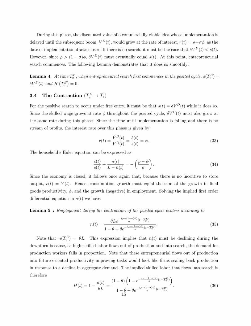
Suppose implementation occurs at discrete dates denoted by T� where v 2 f1; 2; :::;1g. We adoptthe convention that the vth cycle starts at time Tv�1 and ends at time T� . The posited behavior

of entrepreneurs over this cycle is illustrated in Figure 1. After implementation at date Tv�1 there

is an interval during which there is no entrepreneurial search and consequently all managers are

used to supervise production. At some time TEv ; search commences again as the economy begins

11

to decline. Innovative activity is allocated symmetrically across sectors which have not yet had a

success in the current cycle. Once a success occurs, all innovative activity ceases in the sector and

the successful entrepreneur enters production displacing the existing incumbent. Implementation

of the productivity improvement is, however, withheld until time Tv.

Tv1 TE Tv

ImplementationBoom

ImplementationBoom

Expansion Downturn

Zero Entreprenurial SearchIncreasing Search and EntryZero Implementation

vTime

Figure 1: Search, entry and implementation over the cycle

3.2 Within�Cycle Implications

Lemma 1 An incumbent �rm using a technology which is certain to be replaced at the end of

the cycle cannot pro�tably produce using the large scale mode of production.

A �rm in a sector where a new idea is about to be implemented with probability 1 cannot

maintain a relational contract with production workers since it cannot promise employment into

the future. Its production is thus taken over by the newly successful entrepreneur whose termi-

nation date, though not yet known with certainty, will at least not occur before the next cyclical

downturn. Its lowest cost competitors are the competitive fringe who, though producing at small

scale, can in aggregate, steal the new incumbent�s whole market if too high a price is charged.

These competitors avoid the costs of setting up large scale production and hiring multiple work-

ers, but can only produce using the previous state of the art technology. The limit price charged

by intermediate producer i is therefore

pi(t) =s(t)

e� ai(t): (23)

It follows from (2), (4) and (23), that the skilled work force receives a constant share of output:

s(t)(1�H(t)) = e�

�LY (t): (24)

12

It also follows that the pro�ts of an intermediate producer can be expressed as

� (wi(t); t) =

�1� e�

�L� e� wi(t)

s(t)

�Y (t): (25)

Note that, since all sectors face the same skilled salary s (t) and revenue shares are symmetric,

pro�ts vary across sectors only due to di¤erences in the production wage, wi(t). A �nal implication

is that, in equilibrium, the managerial salary is tied to the level of technology. Since within the

posited cycle, the state of intermediate technology in use is unchanging, it follows that

Lemma 2 Within the posited cycle, the managerial salary grows at the rate of technological

change in the �nal output sector:_s(t)

s(t)= �: (26)

Utilizing the incentive compatibility condition (19) ; and the time-varying net present value of

each of the three possible employment states Eij(t); Sij(t) and

Uj (t) yields the following binding

incentive compatible wage for production workers within the posited cycle.

Lemma 3 : The production wage in sector i is given by

wi(t) = �un(t)

uc(t)

�1 +

1

q

��+ �i(t) + �(t)�

_un(t)

un(t)

��: (27)

This expression summarizes the key forces acting on the incentive compatible production wage.

If q !1, then detection of shirking becomes perfect, so that the incentive problem disappears,

and the expression simpli�es to the standard �rst�order condition for household labor supply:

wi(t) = �un(t)=uc(t). In this case, the wage is determined by two forces, both of which arepro�cyclical. As n(t) rises during an expansion the marginal utility cost to the household of

supplying additional workers rises, so that a higher wage is needed to induce this supply. Also,

as consumption c(t) rises the marginal bene�t of supplying additional labor falls, so that �rms

must raise wages to induce labor e¤ort.

However, imperfect detection (q �nite) of shirking introduces three other forces. One of

these is pro�cyclical � as the hiring rate, �(t); rises, being �red is a less costly threat, so that

�rms must raise the wage to provide greater incentives not to shirk. However, the other two

forces are counter-cyclical. First, a higher rate of separation, �i(t); implies that workers must be

compensated for the increased likelihood of job loss.15 Second, with negative employment growth,

the marginal cost of supplying e¤ort is lower tomorrow than today _un(t)=un(t) > 0. Other things

15This positive impact on incentive compatible wages of increased job loss chances has been noticed before insimilar relational contract frameworks by Saint-Paul (1996), and Fella (2000), with evidence consistent with thisbeing found in Abowd and Ashenfelter (1981), Adams (1985) and Li (1986).

13

equal, this makes workers more willing to risk unemployment by shirking, so �rms must raise

wages to compensate.

3.3 The Expansion (Tv�1 ! TEv )

Since all managers are used in production in the expansion of the posited cycle, it must be the

case that production worker employment is at its maximum:

n(t) = �L: (28)

Let the level of output immediately following the boom be given by Y0(Tv�1).16 With a con-

stant level of employment it follows that output grows during the expansion at the rate �, so

that Y (t) = e�(t�Tv�1)Y0(Tv�1). Since the economy is closed, and there is no incentive to store

either intermediate or �nal output across periods (provided r(t) � 0), it must be the case that

consumption grows at this rate too:

_c(t)

c(t)=_Y (t)

Y (t)= �: (29)

Substituting these facts into (16) yields the implied interest rate during the expansion,

r(t) = �+ ��: (30)

Since there is no �rm turnover, �ows out of employment are given by the exogenous sepa-

ration rate ��: Using (6) and (28), it follows that the rate at which workers are hired from the

unemployment pool is then given by�� =

��

1� � (31)

Substituting these facts into (27) implies that the production wage also grows at the rate � during

the expansion:

Proposition 1 : During the expansion of the posited cycle unemployment is constant at (1��)Land the production wage is given by

wA(t) =A

Le�(t�Tv�1)Y0(Tv�1) (32)

where A = �� (1� �)�+ q + ��

1��

�.[(1� �)(1� �)q] :

16Throughout, we use the subscript 0 to denote the value of a variable immediately after the boom. Formally,X0(T ) = limt!T+ X(t).

14

During this phase, the discounted value of a commercially viable idea whose implementation is

delayed until the subsequent boom, V D(t), would grow at the rate of interest, r(t) = �+��; as the

date of implementation draws closer. If there is no search, it must be the case that �V D(t) < s(t):

However, since � > (1 � �)�, �V D(t) must eventually equal s(t). At this point, entrepreneurial

search commences. The following Lemma demonstrates that it does so smoothly:

Lemma 4 At time TEv ; when entrepreneurial search �rst commences in the posited cycle, s(TEv ) =

�V D(t) and H�TEv�= 0.

3.4 The Contraction (TEv ! Tv)

For the positive search to occur under free entry, it must be that s(t) = �V D(t) while it does so.

Since the skilled wage grows at rate � throughout the posited cycle, �V D(t) must also grow at

the same rate during this phase. Since the time until implementation is falling and there is no

stream of pro�ts, the interest rate over this phase is given by

r(t) =_V D(t)

V D(t)=_s(t)

s(t)= �: (33)

The household�s Euler equation can be expressed as

_c(t)

c(t)+

_n(t)

L� n(t) = ��

�: (34)

Since the economy is closed, it follows once again that, because there is no incentive to store

output, c(t) = Y (t). Hence, consumption growth must equal the sum of the growth in �nal

goods productivity, �, and the growth (negative) in employment. Solving the implied �rst order

di¤erential equation in n(t) we have:

Lemma 5 : Employment during the contraction of the posited cycle evolves according to

n(t) =�Le�

(��(1��)�)�

(t�TEv )

1� � + �e�(��(1��)�)

�(t�TEv )

: (35)

Note that n(TEv ) = �L. This expression implies that n(t) must be declining during the

downturn because, as high�skilled labor �ows out of production and into search, the demand for

production workers falls in proportion. Note that these entrepreneurial �ows out of production

into future oriented productivity improving tasks would look like �rms scaling back production

in response to a decline in aggregate demand. The implied skilled labor that �ows into search is

therefore

H(t) = 1� n(t)

�L=(1� �)

�1� e�

(��(1��)�)�

(t�TEv )�

1� � + �e�(��(1��)�)

�(t�TEv )

: (36)

15

The proportion of sectors in which no viable productivity improvement has been identi�ed by

time t 2 (TEv ; Tv) is given by

P (t) = exp

�Z t

TEv

�h(�)d�

!: (37)

Recalling that labor is only devoted to search in sectors where no ideas has been identi�ed, the

labor allocated to search in those sectors is

h(t) =H(t)

P (t): (38)

In the measure (1�P (t)) of sectors where new employers have already entered, the only sourceof separation is normal turnover, ��. However, in sectors where no such restructuring has occurred

yet, the rate of separation also includes the probability of a restructuring occurring, �h(t); which

increases as the downturn proceeds. It follows that the aggregate rate of job destruction is given

by

�A(t) = (1� P (t))��+ P (t)��+ �

H(t)

P (t)

�= ��+ �H(t) (39)

In sectors where entry has already occurred, wages are lower, denoted by wL (t) ; as there is

no chance of further restructuring in the contraction, and so

wL (t) =�c(t)

(1� �)(L� n(t))

�1 +

1

q

��+ ��+ �(t)� _un(t)

un(t)

��: (40)

When a restructuring has not yet occurred, there is higher probability of job destruction and a

higher wage is required to ensure incentive compatibility:

wH (t) =�c(t)

(1� �)(L� n(t))

�1 +

1

q

��+ ��+ �H (t) + �(t)� _un(t)

un(t)

��: (41)

Intuitively, this is because new entrants have a longer expected duration of incumbency than

existing �rms, and can thus promise non-shirking workers a longer expected span of employ-

ment. Recall that free mobility of labor does not equalize wages across these sectors as incentive

compatibility binds.

Since the production wage in each sector is linearly related to the rate of job destruction, it

follows that the average production wage is simply given by (27) with �(t) = �A(t). Substituting

in for the endogenous variables yields the following result:

Proposition 2 : During the contraction of the posited cycle, the average production wage is

given by

wA(t) =

"Be�

��(1��)��

(t�TEv ) � Ce�2(��(1��)�)

�(t�TEv ) +

De��(1��)�

�(t�TEv )

1� � + �e��(1��)�

�(t�TEv )

#e�(t�Tv�1)Y0

L

(42)

where B = �(q+�+��)(1��)(1��)q ; C =

�(�� 1�� )

(1��)(1��)q and D = ��(1��)�(1��)q :

16

The evolution of the production wage during downturns is ambiguous due to the interaction of

the various pro�and counter�cyclical forces mentioned earlier. However, as we document below,

in general the wage traces out a hump�shaped pattern. If counter-cyclical forces dominate, the

wage rises to begin with, largely re�ecting the rising rate of separation. However, as the downturn

proceeds, more and more sectors are taken over by new entrants who then pay the relatively low

wage, wL(t), and fewer sectors are left facing imminent exit and paying the wage wH(t). If the

downturn continues for long enough, this change in sectoral composition, eventually drives down

the average wage.

3.5 The Boom

The growth in aggregate productivity during period Tv is given by

�v =

Z 1

0[ln ai(Tv)� ln ai(Tv�1)] di (43)

Productivity growth at the boom is given by �v = (1� P (Tv)) , where P (Tv) is de�ned by (37).Substituting in the allocation of labor to entrepreneurship through the downturn given by (36)

and integrating over the interval

�Ev = Tv � TEv : (44)

yields the following implication:

Proposition 3 The growth in productivity during the boom of the posited cycle is given by

�v = � �Ev +��

(�� (1� �)�)� ln�1� �

�1� e�

(��(1��)�)�

�Ev��

: (45)

Equation (45) tells us how the size of the productivity boom depends positively on the amount of

time the economy is in the search phase, �Ev . The amount of search in that phase is determined

by the movements in the interest rate, so once the length of the contraction is known, the growth

rate over the cycle is pinned down. The size of the boom is convex in �Ev , re�ecting the fact that

as the boom approaches, search e¤ort increases.

During the boom, productivity and production employment both rise rapidly. Since it is the

product of these two, consumption also increases discontinuously. For this to be consistent with

optimal household behavior, it follows that the discount factor must also rise discontinuously.

The long run discount factor during the boom is given by the household�s Euler equation

R0(Tv)�R(Tv) = � lnc0(Tv)

c(Tv)� � ln L� n0(Tv)

L� n(Tv): (46)

17

Since consumption growth at the boom results both from implementation and the reallocation of

labor into production it follows that

R0(Tv)�R(Tv) = ��v + � lnn0(Tv)

n(Tv)� � ln L� n0(Tv)

L� n(Tv): (47)

Now, n0(Tv) = �L and using (35) to determine n(Tv), we get

R0(Tv)�R(Tv) = ��v + (�� (1� �)�)�Ev : (48)

Over the boom, the asset market must simultaneously ensure that entrepreneurs holding viable

ideas are willing to implement immediately (and no earlier) and that, for households, holding

equity in �rms dominates holding claims to alternative assets (particularly stored intermediates).

The following Proposition demonstrates that these conditions imply that during the boom, the

discount factor must equal productivity growth:

Proposition 4 : Asset market clearing at the boom of the posited cycle requires that

R0(Tv)�R(Tv) = �v (49)

Combining (48) with (49) yields

�v =(�� (1� �)�)�Ev

1� � : (50)

Combining (45) and (50) yields a unique (non�zero) equilibrium pair (�;�E) that is consistent

with the within�cycle dynamics and asset market clearing. Note that although we did not impose

any stationarity on the cycles, the equilibrium conditions imply stationarity of the size of the boom

and the length of the downturn. Existence of such a pair requires that 0 < ��(1��)� < � (1��).

4 Optimal Entrepreneurial Behavior

This section derives a set of su¢ cient conditions under which the behavior posited in Figure 1 is

optimal given the implied behavior of aggregates derived above.

4.1 Optimal Restructuring

The present value of pro�ts earned in a sector where no future entry/exit is anticipated up to the

end of the current cycle is

V � (t) =

Z Tv+1

te�

R �t r(s)ds�(wL(�); �)d�

18

In the cyclical equilibrium considered here, secrecy can be a valuable option.17 Since ideas are

withheld until a common implementation time, simultaneous implementation is feasible. How-

ever, as the following proposition demonstrates, such duplications do not arise in the cyclical

equilibrium because successful entrepreneurs enter production to displace previous incumbents,

sending a credible signal that directs subsequent entrepreneurial e¤orts to sectors other than their

own. The formal details of the signalling game between incumbent, successful entrants, and other

potential innovators are relegated to the appendix.

Proposition 5 : Given that innovations are implemented at the subsequent boom, a success-

ful entrepreneur transfers V � (t) to use the incumbent�s technology until Tv+1; and takes over

production in that sector. All search in their sector then stops until the next cycle.

The payment V � (t) by a successful entrepreneur to the previous incumbent acts as a credible

signal that this entrepreneur has had an innovation, but does not reveal the content of that

success.18 If an entrepreneur�s announcement is credible, other entrepreneurs will exert their

e¤orts in sectors where they have a chance of becoming the sole dominant entrepreneur. One

might imagine that unsuccessful entrepreneurs would have an incentive to mimic successful ones

by falsely announcing success to deter others from entering the sector. But doing this yields a

�ow of pro�ts for the interval t! Tv+1 which is " less than paid for it, and is thus not worthwhile.

It follows that the value of an incumbent �rm in a sector where no innovation has occurred

by time t during the vth cycle can be expressed as

V I(t) =

Z Tv+1

te�

R �t [r(s)+�hi(s)]ds

��(wH(�); �) + �h(�)V �(�)

�d�+

P (Tv+1)

P (t)e�[R0(Tv)�R(t)]V I0 (Tv+1):

(51)

The �rst term here represents the expected discounted pro�t stream that accrues to the entre-

preneur during the current cycle, and the second term is the expected discounted value of being

an incumbent thereafter. Note that due to symmetry, the probability that no innovation arises

between time t and the end of the cycle in any given sector, P (Tv+1)P (t) , is equal to the fraction of

sectors that innovate between t and Tv+1.17As Cohen, Nelson and Walsh (2000) document, delaying implementation to protect knowledge is a widely

followed practice in reality. Graham (2004) also describes a similar critical role of secrecy in protecting value.Scarromozino, Temple and Vulkan (2005) suggest indirect evidence of delay can be gleaned from Hobijn andJovanovic�s (2001) evidence of major changes in US stock valuations anticipating productivity changes. Also,Pastor and Veronesi (2005) provide evidence arguing that the state of the macro economy determines decisions onIPO timing. This is also in line with delay playing a key role.18The payment does not have to be a literal transfer for technology but would instead more realistically take

the form of the entrant renting the incumbent�s machines, plant and production methods for the remainder of therecession. For example, this could occur at a �re-sale over the incumbent �rm�s assets. After that, the entrant willimplement his own methods so that the rental rate on such equipment is zero anyway. The important point is thatthe purchase of the assets at a price that would only be worthwhile to an entrant with a valuable innovation sendsa credible signal to other innovators that pro�ts will be higher if innovations are targetted elsewhere.

19

4.2 Optimal Search and Implementation

The willingness of entrepreneurs to delay implementation until the boom and to just start engag-

ing in search at exactly TEv depends crucially on the expected value of monopoly rents relative

to the current skilled labor returns. This is a forward looking condition: given � and �E , the

present value of these rents depend on the length of the subsequent cycle, Tv+1 � Tv, which we

denote by the term �v+1:

The expected value of an entrepreneurial success occurring at some time t 2�TEv ; Tv

�but

whose implementation is delayed until time Tv is thus:

V D(t) = e�[R0(Tv)�R(t)]V I0 (Tv): (52)

Since Lemma 4 implies that entrepreneurship starts at TEv ; free entry into entrepreneurship,

requires that

�V D(TEv ) = �e�[R0(Tv)�R(TEv )]V I0 (Tv) = s(TEv ): (53)

The increase in the wage across cycles re�ects the improvement in overall productivity: s(TEv+1) =

e�+�v�s(TEv ), and from the asset market clearing conditions, we know that R0(Tv) � R(TEv ) =

�+��E is a constant across cycles. It immediately follows that the increase in the present value

of monopoly pro�ts from the beginning of one cycle to the next must satisfy:

V I0 (Tv) = e�+�v�V I0 (Tv�1): (54)

The following proposition demonstrates that (54) implies a unique cycle length:

Proposition 6 Given the boom size, �, and the length of the downturn, �E, there exists a

unique cycle length, �, such that entrepreneurs are just willing to commence search �E periods

prior to the boom.

The length of the cycle is given by

� = �E +1

bln

241 + ��E + �1 �1� e� b��E�� 2

�1� e�

2b��E��

�3

�1� e� b

��E�

1� ��1� e� b

��E�35 ; (55)

where b = � + (1 � �)� and �; �1; �2 and �3 are positive constants. Notice, once again that

stationarity is not imposed, but is implied by the equilibrium conditions.

The equilibrium conditions (20), (21) and (22) on posited entrepreneurial behavior also impose

the following requirements on our hypothesized cycle:

20

� Entrepreneurs with commercially viable ideas at time t = Tv, must prefer to implement imme-

diately, rather than delay:

V I0 (Tv) > V D0 (Tv): (56)

This condition is also su¢ cient to ensure that household utility is bounded in equilibrium, since

it implies that191

�ln

�c0(Tv)

c0(Tv�1)

�=�

�+ � <

�

1� � : (57)

From (50) this condition must hold if � > �E :

� Entrepreneurs who identify commercially viable ideas during the downturn must prefer to waituntil the beginning of the next cycle rather than implement earlier:

V I(t) < V D(t) 8 t 2 (TEv ; Tv) (58)

� No entrepreneur wants to innovate during the expansion of the cycle. Since in this phase of thecycle �V D(t) < s(t), this condition requires that

�V I(t) < s(t) 8 t 2 (Tv�1; TEv ) (59)

In constructing the equilibrium we have implicitly imposed two additional requirements:

� The downturn is not long enough that all sectors innovate:

P (Tv) > 0: (60)

� Firm operating pro�ts are always positive:

�i(t) > 0 8 i, t (61)

5 Baseline Example

In this section we demonstrate that the triple (�E ;�;�) > 0 solving (45), (50), (55) exists, and

the conditions (E1) through (E5) are satis�ed. For these values, posited entrepreneurial behavior

is optimal given the implied cyclical behavior of aggregates that are generated by this behavior,

so that the cycling steady state exists. We do this by �rst solving the model for a baseline set

19To see this observe that (E1) can be expressed as V I0 (Tv) > e

�[R0(Tv+1)�R0(Tv)]e�+��V I0 (Tv); which holds only

if R0(Tv+1)�R0(Tv) = � (� + ��) + �� > � +��. Re-arranging yields (57).

21

of parameters, and then vary these. This exercise is not an attempt to assess the quantitative

signi�cance of the model. Rather, our aim here is instead to establish that the existence conditions

can be simultaneously satis�ed for values that are within reasonable bounds. The second aim is

to gain some understanding of the model�s comparative static properties by varying parameters

around this baseline case.

Table 1 documents the parameters used for our baseline case. These parameters were chosen

so that the model generates a long�run growth rate of close to 2%, a cycle length of about 10 years

and a correlation of de�trended log average wages and log output close to zero. The length of an

expansion, �X ; is 7.10 years and of a contraction, �E ; is 2.88 years in this baseline. Figure 2

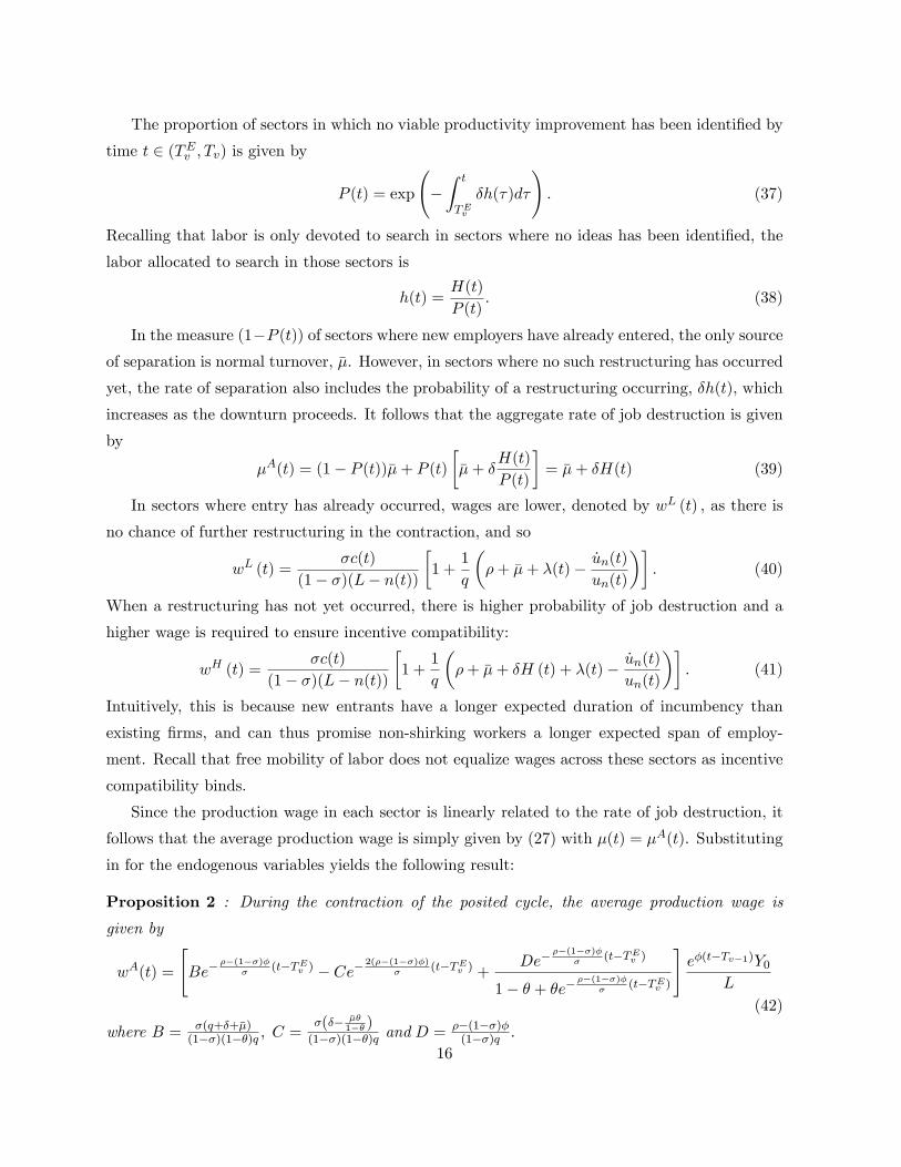
illustrates the evolution of key aggregates over a cycle implied by simulating the baseline example.

After rising gradually during the expansion, output falls rapidly in the contraction. However,

correctly measured GDP should include the payments made to labour used in entrepreneurial

search. As illustrated, GDP also falls during the downturn, but less rapidly. The reason GDP

falls is that skilled labor used in production is being paid below its marginal product. As labour

e¤ort is transferred into search, the marginal cost in terms of lost output exceeds the marginal

bene�t of search. Because it is o¤set by the fall in this intangible investment, the rise in GDP at

the boom is also less dramatic than otherwise.

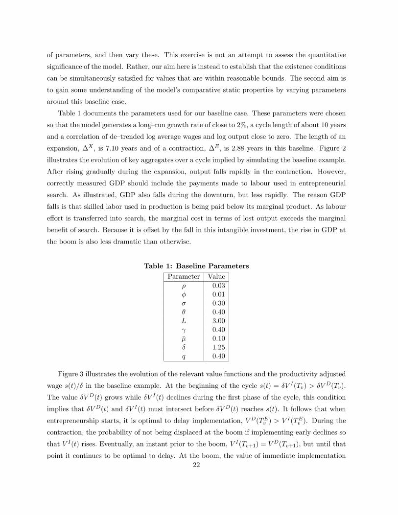
Table 1: Baseline ParametersParameter Value

� 0.03� 0.01� 0.30� 0.40L 3.00 0.40�� 0.10� 1.25q 0.40

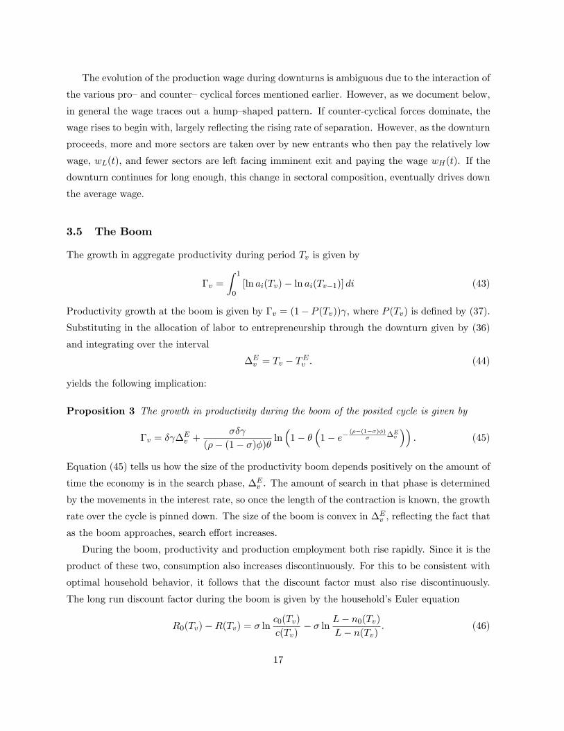
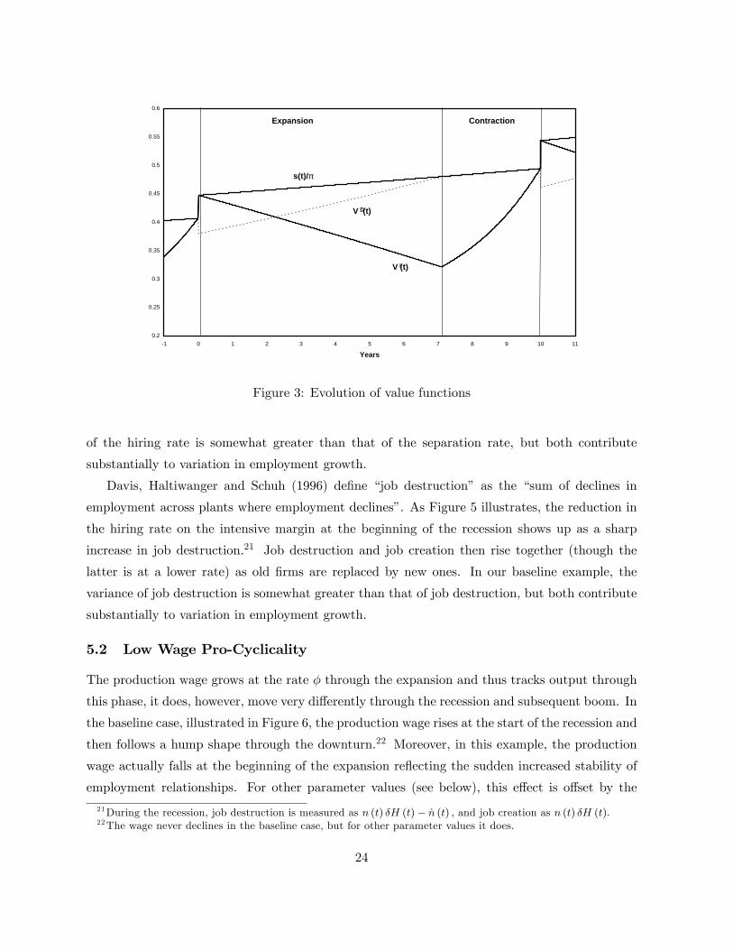
Figure 3 illustrates the evolution of the relevant value functions and the productivity adjusted

wage s(t)=� in the baseline example. At the beginning of the cycle s(t) = �V I(Tv) > �V D(Tv).

The value �V D(t) grows while �V I(t) declines during the �rst phase of the cycle, this condition

implies that �V D(t) and �V I(t) must intersect before �V D(t) reaches s(t). It follows that when

entrepreneurship starts, it is optimal to delay implementation, V D(TEv ) > V I(TEv ). During the

contraction, the probability of not being displaced at the boom if implementing early declines so

that V I(t) rises. Eventually, an instant prior to the boom, V I(Tv+1) = V D(Tv+1), but until that

point it continues to be optimal to delay. At the boom, the value of immediate implementation22

rises, while the value of delayed implementation falls, so that all existing innovations are imple-

mented. However, since the skilled wage increases by as much as V I(t), search ceases and the

cycle begins again.

0

0.2

0.4

0.6

0.8

1

1.2

1.4

1.6

1 0 1 2 3 4 5 6 7 8 9 10 11

Years

Out

put,

wag

es

0

2

4

6

8

10

12

14

Inte

rest

rate

(%)

Output

GDP

Managerial Wage

Interest Rate

Expansion Contraction

Figure 2: Evolution of some key variables over the cycle

5.1 Restructuring: Intensive and Extensive Margin Adjustment

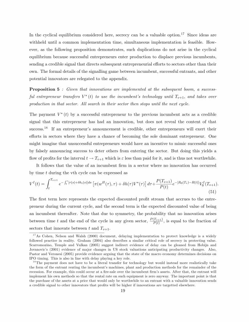
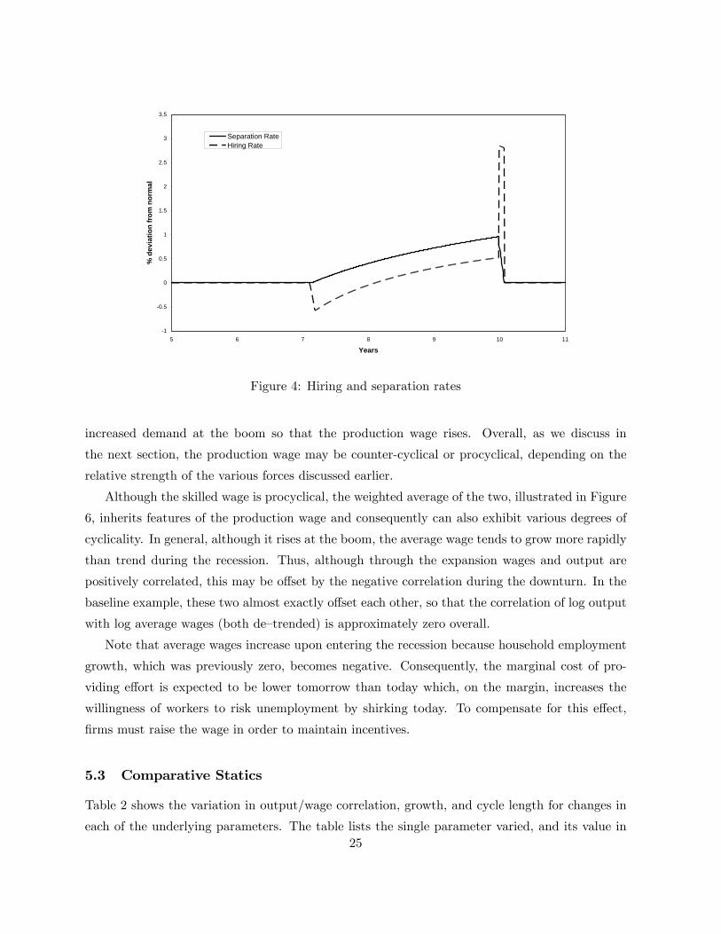
The pattern of average hiring and separation rates implied by this baseline case are plotted in

Figure 4. Both are stable through the expansion and only occur because of turnover on the

intensive margin, ��. Upon entering the contractionary phase, the hiring rate falls as �rms cut

back on the intensive margin in response to falling aggregate demand. This is generated by

the endogenous recession occurring through increased restructuring. Simultaneously, the steady

increase in entrepreneurial search leads to increasing job separation through this phase on the

extensive margin; old �rms are being driven out of production by new ones. Entry is also re�ected

in the gradual but steady pick up in the hiring rate that starts to occur in anticipation of the

forthcoming boom. At the boom, existing �rms then adjust employment on the intensive margin,

increasing employment to meet the increased aggregate demand. This leads to a surge in hiring

and an increase in employment which starts o¤the next cycle.20 As Figure 4 suggests, the variance20As in the data, we measure hiring and separation at monthly intervals. Consequently, the discontinuity in the

hiring rate at the boom shows up as a dramatic, but �nite increase in hiring.

23

0.2

0.25

0.3

0.35

0.4

0.45

0.5

0.55

0.6

1 0 1 2 3 4 5 6 7 8 9 10 11

Years

s(t)/π

V (t)

V (t)

D

I


Figure 3: Evolution of value functions

of the hiring rate is somewhat greater than that of the separation rate, but both contribute

substantially to variation in employment growth.

Davis, Haltiwanger and Schuh (1996) de�ne �job destruction� as the �sum of declines in

employment across plants where employment declines�. As Figure 5 illustrates, the reduction in

the hiring rate on the intensive margin at the beginning of the recession shows up as a sharp

increase in job destruction.21 Job destruction and job creation then rise together (though the

latter is at a lower rate) as old �rms are replaced by new ones. In our baseline example, the

variance of job destruction is somewhat greater than that of job destruction, but both contribute

substantially to variation in employment growth.

5.2 Low Wage Pro-Cyclicality

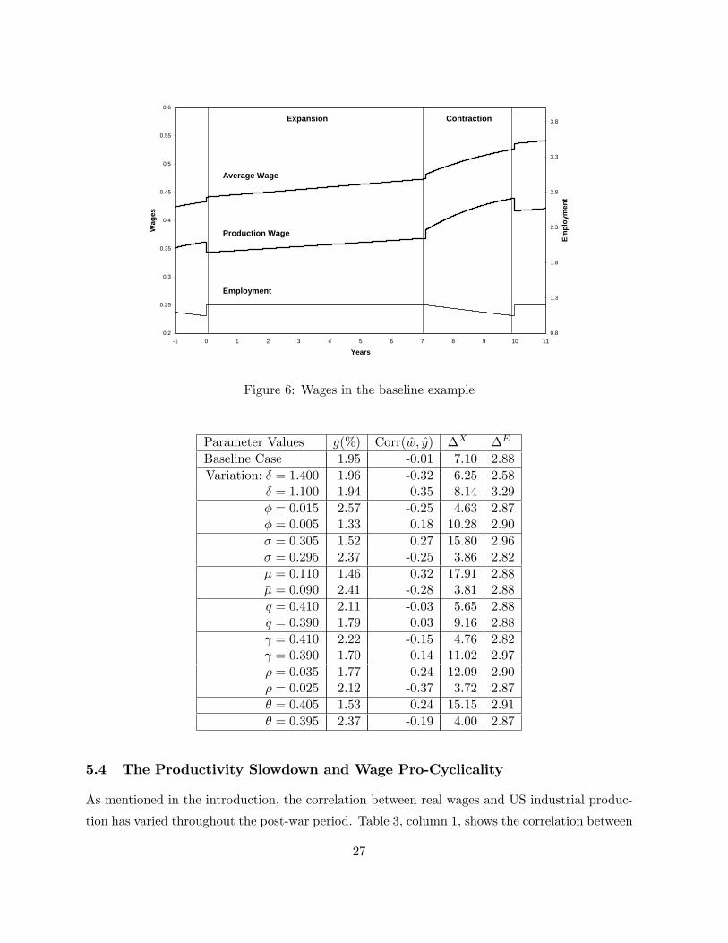
The production wage grows at the rate � through the expansion and thus tracks output through

this phase, it does, however, move very di¤erently through the recession and subsequent boom. In

the baseline case, illustrated in Figure 6, the production wage rises at the start of the recession and

then follows a hump shape through the downturn.22 Moreover, in this example, the production

wage actually falls at the beginning of the expansion re�ecting the sudden increased stability of

employment relationships. For other parameter values (see below), this e¤ect is o¤set by the

21During the recession, job destruction is measured as n (t) �H (t)� _n (t) ; and job creation as n (t) �H (t).22The wage never declines in the baseline case, but for other parameter values it does.

24

1

0.5

0

0.5

1

1.5

2

2.5

3

3.5

5 6 7 8 9 10 11

Years

% d

evia

tion

from

nor

mal

Separation RateHiring Rate

Figure 4: Hiring and separation rates

increased demand at the boom so that the production wage rises. Overall, as we discuss in

the next section, the production wage may be counter-cyclical or procyclical, depending on the

relative strength of the various forces discussed earlier.

Although the skilled wage is procyclical, the weighted average of the two, illustrated in Figure

6, inherits features of the production wage and consequently can also exhibit various degrees of

cyclicality. In general, although it rises at the boom, the average wage tends to grow more rapidly

than trend during the recession. Thus, although through the expansion wages and output are

positively correlated, this may be o¤set by the negative correlation during the downturn. In the

baseline example, these two almost exactly o¤set each other, so that the correlation of log output

with log average wages (both de�trended) is approximately zero overall.

Note that average wages increase upon entering the recession because household employment

growth, which was previously zero, becomes negative. Consequently, the marginal cost of pro-

viding e¤ort is expected to be lower tomorrow than today which, on the margin, increases the

willingness of workers to risk unemployment by shirking today. To compensate for this e¤ect,

�rms must raise the wage in order to maintain incentives.

5.3 Comparative Statics

Table 2 shows the variation in output/wage correlation, growth, and cycle length for changes in

each of the underlying parameters. The table lists the single parameter varied, and its value in25

0.1

0

0.1

0.2

0.3

0.4

0.5

0.6

0.7

0.8

5 6 7 8 9 10 11

Years

Ann

ualiz

ed ra

tes

DHS: DestructionDNS: Creation

Figure 5: Job Creation and Destruction using de�nition of Davis et al. (1996)

the �rst column with the endogenous results in the columns to the immediate right. The intuition

for most of the comparative static results in the table is relatively straightforward. Changes in

parameters that reduce incentives to engage in entrepreneurial search: lowering � or (which

have direct e¤ect on returns to search e¤ort); lowering q and raising � (which raises the e¢ ciency

wage, thereby lowering pro�ts); raising � and � (which makes consumers less willing to delay

consumption) all lower the growth rate, as one would expect in a model of endogenous growth.

Most of these changes also leave the length of the economy�s contraction relatively unchanged,

but imply (sometimes large) changes in the length of expansions. This is because with weaker

fundamental incentives to search for productivity improvements, longer expansionary phases, and

therefore a longer reign of incumbency and pro�t, are required to provide su¢ cient incentives for

entrepreneurship.

Table 2: Growth, Wage Cyclicality, and Cycle Lengths

26

0.2

0.25

0.3

0.35

0.4

0.45

0.5

0.55

0.6

1 0 1 2 3 4 5 6 7 8 9 10 11

Years

Wag

es

0.8

1.3

1.8

2.3

2.8

3.3

3.8

Empl

oym

ent

Production Wage

Average Wage

Employment


Figure 6: Wages in the baseline example

Parameter Values g(%) Corr(w; y) �X �E

Baseline Case 1.95 -0.01 7.10 2.88Variation: � = 1:400 1.96 -0.32 6.25 2.58

� = 1:100 1.94 0.35 8.14 3.29� = 0:015 2.57 -0.25 4.63 2.87� = 0:005 1.33 0.18 10.28 2.90� = 0:305 1.52 0.27 15.80 2.96� = 0:295 2.37 -0.25 3.86 2.82�� = 0:110 1.46 0.32 17.91 2.88�� = 0:090 2.41 -0.28 3.81 2.88q = 0:410 2.11 -0.03 5.65 2.88q = 0:390 1.79 0.03 9.16 2.88 = 0:410 2.22 -0.15 4.76 2.82 = 0:390 1.70 0.14 11.02 2.97� = 0:035 1.77 0.24 12.09 2.90� = 0:025 2.12 -0.37 3.72 2.87� = 0:405 1.53 0.24 15.15 2.91� = 0:395 2.37 -0.19 4.00 2.87

5.4 The Productivity Slowdown and Wage Pro-Cyclicality

As mentioned in the introduction, the correlation between real wages and US industrial produc-

tion has varied throughout the post-war period. Table 3, column 1, shows the correlation between

27

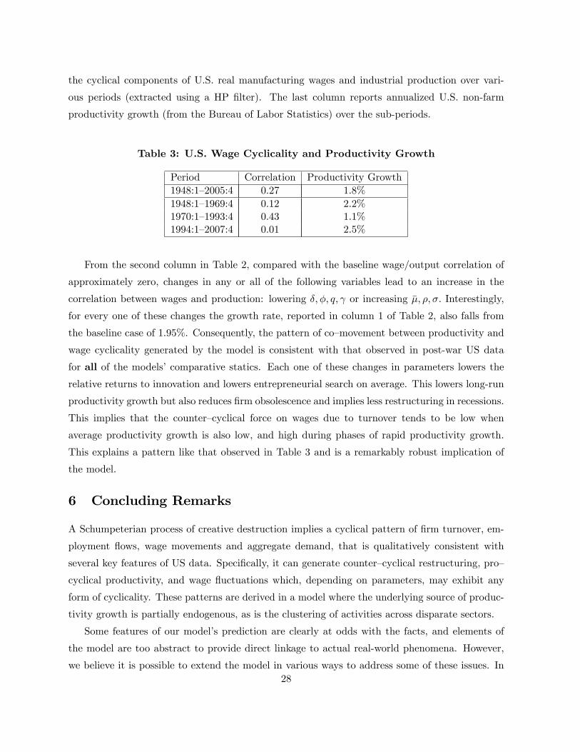
the cyclical components of U.S. real manufacturing wages and industrial production over vari-

ous periods (extracted using a HP �lter). The last column reports annualized U.S. non-farm

productivity growth (from the Bureau of Labor Statistics) over the sub-periods.

Table 3: U.S. Wage Cyclicality and Productivity Growth

Period Correlation Productivity Growth1948:1�2005:4 0.27 1.8%1948:1�1969:4 0.12 2.2%1970:1�1993:4 0.43 1.1%1994:1�2007:4 0.01 2.5%

From the second column in Table 2, compared with the baseline wage/output correlation of

approximately zero, changes in any or all of the following variables lead to an increase in the

correlation between wages and production: lowering �; �; q; or increasing ��; �; �: Interestingly,

for every one of these changes the growth rate, reported in column 1 of Table 2, also falls from

the baseline case of 1.95%. Consequently, the pattern of co�movement between productivity and

wage cyclicality generated by the model is consistent with that observed in post-war US data

for all of the models�comparative statics. Each one of these changes in parameters lowers the

relative returns to innovation and lowers entrepreneurial search on average. This lowers long-run

productivity growth but also reduces �rm obsolescence and implies less restructuring in recessions.

This implies that the counter�cyclical force on wages due to turnover tends to be low when

average productivity growth is also low, and high during phases of rapid productivity growth.

This explains a pattern like that observed in Table 3 and is a remarkably robust implication of

the model.

6 Concluding Remarks

A Schumpeterian process of creative destruction implies a cyclical pattern of �rm turnover, em-

ployment �ows, wage movements and aggregate demand, that is qualitatively consistent with

several key features of US data. Speci�cally, it can generate counter�cyclical restructuring, pro�

cyclical productivity, and wage �uctuations which, depending on parameters, may exhibit any

form of cyclicality. These patterns are derived in a model where the underlying source of produc-

tivity growth is partially endogenous, as is the clustering of activities across disparate sectors.

Some features of our model�s prediction are clearly at odds with the facts, and elements of

the model are too abstract to provide direct linkage to actual real-world phenomena. However,

we believe it is possible to extend the model in various ways to address some of these issues. In28

particular, the productivity boom and the associated jump in job creation are rather abrupt. As

we show in Francois and Lloyd�Ellis (2008), adding capital can help to smooth out the boom to

some extent. If capital and production labor are strong complements in the short run, job creation

may then be relatively slow following the boom. Another unrealistic feature of the cyclical process

that we generate is that every cycle is the same and all �uctuations are deterministic. Extending

the model to allow for some stochastic elements would relax some of these strong predictions.

One approach that we are exploring is to allow the exogenous component of productivity growth

to be subject to temporary i.i.d. shocks. This can change the length and amplitude of each cycle

without changing the basic story.

In this paper, the search for commercially viable ideas and productivity improvements is a

counter�cyclical form of innovative activity. Indeed, there is some evidence that this kind of

innovative activity is undertaken by managers during periods of slack demand. For example,

Nickell, Nicolitsas and Patterson (2001) �nd that �managerial innovations�� changes in struc-

ture; organization leaner as result of change; signi�cant changes resulting in more decentralized

organization; signi�cant changes in human resources management practices and industrial rela-

tions; the implementation of just in time technologies.� are concentrated during in downturns.

In contrast, recent evidence suggests that R&D is procyclical, even for �rms that are not obvi-

ously cash�constrained during downturns (see Barlevy, 2007, and Walde and Woitek, 2004). In

Francois and Lloyd-Ellis (2009) we introduce endogenous R&D as a separate, knowledge-intensive

activity that generates ideas whose commercial viability is unclear. The resulting stock of ideas

can then be drawn upon by manager/entrepreneurs in their search for productivity improve-

ments, and matched with speci�c markets. As in the current paper, entrepreneurial search is

counter-cyclical, but R&D investment is pro-cyclical.

29

Appendix

Proof of Lemma 1: Consider a �rm holding an obsolete technology at time t. For there to

exist a technology better than the �rm�s, an innovator must have allocated h to innovation in

the �rm�s sector. But only �rms planning to implement an innovation will �nd it worthwhile

to undertake innovative e¤ort, consequently, for the new technology, there exists some planned

optimal date at which the technology will be implemented. Denote this date by t�: Using the

large scale of production requires hiring workers who do not shirk. This is only possible if the

wage is incentive compatible. Clearly, at t� the �rm using the obsolete technology is not able to

compete in production, so the large scale of production cannot be used. However it is also the

case that incentive compatibility cannot hold, and the large scale of production not be used, if

employment terminates with probability one in the next instant. Consequently at time t� � dt

it is also not possible to use the large scale technology. However, the same argument applies at

time t� � 2dt since the worker then knows that at t� � dt employment will be terminated. The

same reasoning applies for each instant until time t:

Proof of Lemma 2: From the production function we have ln y(t) = �t +R 10 ln

y(t)pi(t)

di: Substi-

tuting for pi(t) using (23) re-arranges to

s(t) = e� exp

��t+

Z 1

0ln ai(Tv�1)di

�= e�(t�Tv�1)s (Tv�1) : (62)

Proof of Lemma 3: Pro�t maximization implies that Ei (t) = Si (t) � U (t) and so �i (t) =

Ei (t): It follows that the Bellman equation associated with a worker who is employed and not

shirking in sector i is given by

� Ei (t) = (wi(t)uc(t) + un(t))� �i(t)� Ei (t)� U (t)

�+ _

Ei (t) (63)

Similarly the Bellman equations associated with workers who are shirking in sector i and unem-

ployed, respectively, can be expressed as

� Si (t) = wi(t)uc(t)� [�i(t) + q]� Si (t)� U (t)

�+ _

Si (t) (64)

� U (t) = �(t)� Ei (t)� U (t)

�+ _

U(t) (65)

Pro�t maximization subject to the incentive compatibility condition implies that Ei (t) = Si (t)

and so subtracting (63) from (64) we get

Ei (t)� U (t) = �un(t)

q(66)

30

It follows that Ei (t) = E(t) 8i and that

_ E(t)� _

U(t) = � _un(t)

q(67)

Subtracting (65) from (63), substituting using (66) and re-writing yields (27) :�

Proof of Proposition 1: Substituting for c (t) from (29), setting _unun= (1 � �)�; and noting

that when dn = 0 and �A = �; � = ��1�� ; equation (27) rearranges to (32) :

Proof of Lemma 4: Note that in any preceding no-entrepreneurship phase, r (t) = �+��. Thus,

since, in a cycling equilibrium, the date of the next implementation is �xed at Tv; the expected

value of entrepreneurship, �V D; also grows at the rate � + �� > 0: Thus, if under H(TEv ) = 0;

�V D(TEv ) > s(TEv ); then the same inequality is also true the instant before, i.e. at t! TEv , since

s(t) grows at the slower rate, � < � + ��, within the cycle. But this violates the assertion that

entrepreneurship commences at TEv : Thus necessarily, �VD(TEv ) = s(TEv ) at H

�TEv�= 0:

Proof of Proposition 2: From (6) we can express the rate of job creation as

�(t) =�A(t)n(t) + _n(t)

L� n(t) : (68)

Using the fact that �A(t) = ��+ �(1� n(t)=�L) and substituting into (42) yields

wA(t) =�c(t)

(1� �) (L� n(t))q

"�+ q +

�

��

�(1��)� L� ��LL� n(t) +

_n(t)

L� n(t) �_un(t)

un(t)

#(69)

Di¤erentiating (35) yields

_n(t) =� (1� �) ��(1��)�� Le�

��(1��)��

(t�TEv )h1� � + �e�

��(1��)��

(t�TEv )i2 : (70)

Using (83) and (35) we have that

L� n(t) = (1� �)L1� � + �e�

��(1��)��

(t�TEv )(71)

Di¤erentiating (12) w.r.t. time and using (34) to substitute yields

_un(t)

un(t)= �� (1� �)�

�(72)

Noting that c(t) = Y0(Tv�1)e�(t�Tv�1)n(t)=�L; substituting into (69) using (70), (71) and (72)

and re�arranging yields (42).

31

Proof of Proposition 3: Long�run productivity growth is given by

�v = (1� P (Tv)) = �

Z Tv

TEv

H(�)d� (73)

Substituting using (36) and integrating yields (45).

Proof of Proposition 4: Just prior to the boom, when the probability of displacement is

negligible, the value of implementing immediately must equal that of delaying until the boom:

�V I(Tv) = �V D(Tv) = s(Tv): (74)

During the boom V I0 (Tv) > V D0 (Tv). Thus the return to innovation at the boom is the value of

immediate incumbency. It follows that free entry into entrepreneurship at the boom requires that

�V I0 (Tv) � s0(Tv): (75)

The opportunity cost to �nancing entrepreneurship is the rate of return on shares in incumbent

�rms in sectors where no innovation has occurred. Just prior to the boom, this is given by the

capital gains in sectors where no innovations have occurred. Combined with (74) and (75) it

follows that asset market clearing at the boom requires

R0(Tv)�R(Tv) = log�V I0 (Tv)

V I(Tv)

�� log

�s0(Tv)

s(Tv)

�= �v: (76)

Provided that R0(Tv) � R(t) > 0, households will not store �nal output from within a cycle

to the beginning of the next. However, the return on stored intermediate output in sectors with

no innovations is strictly positive because its price increases at the boom. If innovative activities

are to be �nanced at time t; households cannot be strictly better o¤ buying claims to stored

intermediate goods. Consider a sector where no innovation has occurred just prior to the boom.

Since the cost of production is the same whether the good is stored or not, the rate of return on

claims to stored intermediates in sector i is log pi;v+1 =pi;v = �v. It follows that the long run rate

of return on claims to �rm pro�ts an instant prior to the boom must satisfy

R0(Tv)�R(Tv) � log pi;v+1 =pi;v = �v: (77)

Combining (76) and (77) yields the equality in the statement of proposition.

Proof of Proposition 5:

Message space: At "! 0 cost, an innovator targeting sector i, which has not yet had a signal of

search success, can either send a public signal of success Zi (t) = 1; or send no signal in which

32

case Zi (t) = 0: Since search occurs in continuous time we ignore the zero probability event of

more than one innovation arriving simultaneously.

Description of equilibrium behavior : If, and only if, an entrepreneur succeeds he sends a signal

of success immediately. If, and only if, an incumbent sees Zi (t) = 1; he shuts down production.

If, and only if, another entrepreneur targeting sector i sees Zi (t) = 1 he subsequently targets

another sector j in which Zj (t) = 0:

Optimality of signal sender�s equilibrium behavior: During the phase in which search occurs,

V I (t) < V D (t) : Consequently, an entrepreneur would prefer delaying implementation of innova-

tion to time T0: Suppose that at time t an incumbent sees Zi (t) = 1: Then either an entrepreneur

has succeeded and sent a signal, or has not succeeded and is falsely sending a signal of success.

If an entrepreneur has been successful, expected returns when sending the signal are: V D (t)� ":This exceeds the return to immediate implementation, V I (t) :

If the entrepreneur has not been successful, but is sending a signal falsely, then expected

returns to innovation are �V D (t) � ": However, if the false sender of the signal were to follow

the posited equilibrium behavior instead, and delay sending a signal until if and when a success

arrives, then expected returns to search would be ��V D (t)� "

�> �V D (t)� ": Consequently, an

unsuccessful entrepreneur would never falsely send a signal of success, and a successful entrepre-

neur strictly prefers sending a signal of success.

Optimality of recipient�s equilibrium behavior: Given equilibrium described by strategies b� forworkers and incumbents in production, when Zi (t) = 1; the incumbent �rm knows that, in all

subsequent periods, any positive wage o¤er to any worker j will lead to shirking. Consequently

the �rm strictly prefers to shut down production.

Optimality of unsuccessful entrepreneur�s behavior: Given that Zi (t) = 1; a non-innovator con-

jectures that an innovation success has arrived in sector i: Consequently, if the entrepreneur were

to subsequently succeed in sector i, V Di (t) would equal 0; since the entrepreneur would Bertrand

compete with an incumbent holding an identical technology. Consequently, provided there exists

another sector j; with V Dj (t) > 0; and with Zj (t) = 0; the entrepreneur will target sector j

subsequently.

Proof of Proposition 6: Although, during the downturn, the realized pro�ts of �rm di¤er

across sectors, the fact that pro�ts are linear in the production wage implies that expected pro�ts

at time TEv are equivalent to the pro�ts of a �rm that pays the average wage for t 2�TEv ; Tv

�(see

Appendix B for details) This implies that the value of a �rm at time Tv�1 can be expressed as

V I0 (Tv�1) =1�

1� P (Tv)e�v�[R0(Tv)�R(Tv�1)]� Z Tv

Tv�1

e�R �Tv�1

r(s)ds�1� e�

�L� e� w

A(�)

s(�)

�Y (�)d�

33

Substituting in for the endogenous variables, integrating and dividing through by Y0(Tv�1) yields�1� P (Tv)e��[R0(Tv)�R0(Tv�1)]

� V I0 (Tv�1)Y0(Tv�1)

=

�1� e�

�L

�"1� e�b(TEv �Tv�1)

b� e��(TEv �Tv�1)

� �b�ln�1� �

�1� e�

b��E��#

� 1� e��(TEv �Tv�1)

�

!A� (78)

�e�b(TEv �Tv�1)�b

26664�B + 1��

� C� �1� e� b

��E + 1��

� ln�1� �

�1� e� b

��E��

�12C�1� e� 2b

��E��D

0@1� ln

�1� �

�1� e�

��E��+

(1��)�1�e�

b��

E�

1��1�e�

b��

E�1A37775

where b = �� (1� �)�: Noting that �V I0 (Tv�1) = w0(Tv�1) = e� Y0(Tv�1)=�L and substituting

using (45) and (50) we can derive�eb(��

E) � 1�� e�

��L� 1b

�1� e�

�L

�+A�

b

�(79)

=

�(1� e�

�L)� b

� (1� �) +��B +

1� ��

C

�(1� �)�D

��1� b

� (1� �)

��E

��b

24�B + 1� ��

C

��1� e�

b��E�� 12C�1� e�

2b��E��D

(1� �)�1� e� b

��E�

1� ��1� e� b

��E�35

Dividing through byhe�

��L �1b

�1� e�

�L

�+ A�

b

iand solving for � yields (55), where

� =

b� (1��) � (1�

e�

�L )��B + 1��

� C�(1� �)�D

� �1� b

� (1��)

�1b

�1� e�

�L

�� e�

��L �A�b

; (80)

�1 =�b

�B + 1��

� C�

1b

�1� e�

�L

�� e�

��L �A�b

; �2 =�b12C

1b

�1� e�

�L

�� e�

��L �A�b

(81)

and �3 =

�(��(1��)�)D (1� �)

1b

�1� e�

�L

�� e�

��L �A�b

:

34

References

Abraham, K.G. and J.C. Haltiwanger (1995), �Real Wages and the Business Cycle,�Journal of

Economic Literature, Vol. 33, No. 3, 1215-1264.

Abowd, J. and O. Ashenfelter (1981) Anticipated Unemployment, Temporary Layo¤s, and Com-

pensating Wage Di¤erentials, in: S. Rosen ed. Studies in Labor Markets, University of Chicago

Press, Chicago.

Adams, J.D. (1985), �Permanent Di¤erences in Unemployment and Permanent Wage Di¤er-

ences,�Quarterly Journal of Economics, 100, 29-56.

Aghion, Philippe and Peter Howitt (1992) �A Model of Growth Through Creative Destruction,�

Econometrica, vol. 60, pp. 323�351.

Aguirregabiria, Victor and Cesar Alonso-Borrego, �Occupational Structure, Technological Inno-

vation, and Reorganization of Production,�Labour Economics, vol. 8 (1), Jan. 2001, pp. 43-73.

Alexopoulos, Michelle (2004), �Unemployment and the Business Cycle,� Journal of Monetary

Economics (2004) vol. 51, 277-298.

Barlevy, Gadi (2007), �On the timing of innovation in stochastic Schumpeterian growth models,�

American Economic Review, vol. 97 (4), pp. 1131-1164.

Beaudry, Paul, and Franck Portier (2006), �Stock Prices, News and Economic Fluctuations,�

American Economic Review, vol. 96 (4), pp. 1293-1307

Bils, M. (1985) �Real Wages over the Business Cycle: Evidence from Panel Data,� Journal of

Political Economy,

Blanchard, O.J. and P. Diamond (1990), �The cyclical behavior of the gross �ows of US workers,�

Brookings Papers on Economic Activity, 85-155.

Bleakley, H., A. Ferris and J. Fuhrer (1999), �New Data on Worker Flows During Business

Cycles,�New England Economic Review, July/August 1999.

Burgess, S., J. Lane and D. Stevens (2001) �Churning Dynamics: An Analysis of Hires and

Separations at the Employer Level.�Labor Economics 8, 1-14.

Caballero, R. and M. Hammour (1994) �The Cleansing E¤ect of Recessions�American Economic

Review 84(5), December 1994, 1350-1368.

Chang, Yongsung (2000), �Wages, Business Cycles, and Comparative Advantage,� Journal of

Monetary Economics, 46 (1) 143-172.

Cohen, W., R. Nelson and J. Walsh (2000) �Protecting Their Intellectual Assets: Appropriability

Conditions and Why US �rms Patent or Not�NBER # 7552.

Comin, D. (2004), �R&D: A small contribution to productivity growth,� Journal of Economic

Growth, December.

35

Danthine, J.P. and A. Kurman (2004), �Fair wages in a Keynesian model of the business cycle,�

CIRPEE discussion paper 03-02.

Davis, S.J. and J. Haltiwanger (1992), �Gross job creation, gross job destruction and employment

reallocation,�Quarterly Journal of Economics, 107(3) 819-863.

Davis, S.J., J.Haltiwanger and S. Schuh (1996), Job creation and destruction, MIT Press, Cam-

bridge.

De Jong, D. and B. Ingram (2001) �The cyclical behavior of skill acquisition,�Review of Economic

Dynamics, 4(3) 536-561.

den Haan, Wouter J., Garey Ramey and Joel Watson (1999), �Contract-theoretic approaches to

wages and displacement,�Review, Federal Reserve Bank of St. Louis, May, 55-72.

Elsby, Michael, Ryan Michaels and Gary Solon (2009), �The Ins and Outs of Cyclical Unemploy-

ment,�American Economic Journal: Macroeconomics, vol. 1 (1), pp. 84-110.

Fay, Jon-A. and James-L. Medo¤ (1985), �Labor and Output over the Business Cycle: Some

Direct Evidence,�American Economic Review, vol. 75 (4), September 1985, pp. 638-55.

Fella, G. (2000), �E¢ ciency Wage and E¢ cient Redundancy Pay,�European Economic Review,

44, 1473-1490.

Faberman (2008), �Job �ows, jobless recoveries and the Great Moderation,� Federal Reserve

Bank of Philadelphia Working Paper # 08-11.

Francois, P. and H. Lloyd-Ellis (2003), �Animal Spirits Through Creative Destruction,�American

Economic Review, vol. 93 (3), pp. 530-550

Francois, P. and H. Lloyd-Ellis (2008), �Implementation Cycles, Investment and Growth,�Inter-

national Economic Review, vol 49 (3), August 2008, pp. 901-942.

Francois, P. and H. Lloyd-Ellis (2009), �Schumpeterian Business Cycles with Pro-Cyclical R&D,�

Review of Economic Dynamics, vol 12 (4), pp. 567-591.

Fujita, Shigeru and Garey Ramey (2009), �The Cyclicality of separation and job �nding rates,�

International Economic Review, vol. 50 (2), pp. 415-430.

Gomme, Paul (1999), �Shirking, Unemployment and Aggregate Fluctuations,�International Eco-

nomic Review, vol. 40 (1), pp. 3�21.

Graham, S. J. H. (2004) �Patenting in the Shadow of Secrecy: Innovators�Uses of U.S. Patent

O¢ ce Continuation Practice, 1975�2002.� In Continuation, Complementarity, and Capturing

Value: Three Studies Exploring Firms�Complementary Uses of Appropriability Mechanisms in

Technological Innovation. Ph.D. dissertation, University of California, Berkeley.

Grossman, Gene and Elhanan Helpman, Innovation and Growth in the Global Economy, Cam-

bridge, MA.: MIT press, 1991.

Hall, R.E. (2005), �Job Loss, Job Finding and Unemployment in the US Economy over the Past

36

50 Years,�mimeo, Stanford University.

Hobijn, B. and B. Jovanovic (2001) The Information Technology Revolution and the Stock Mar-

ket: Evidence, American Economic Review, 91, 5, 1203-1220.

Li, H.L. (1986) Compensating Di¤erentials for Cyclical and Non-Cyclical Unemployment: The

Interaction Between Investor�s and Employee�s Risk Aversion, Journal of Labor Economics, 4,

277-300.

Macleod, Bentley and James Malcomson (1989), �Implicit Contracts, Incentive Compatibility

and Involuntary Unemployment,�Econometrica 56 447.

Mortensen, Dale T and Christopher A. Pissarides (1994), �Job Creation and Job Destruction in

the Theory of Unemployment,�Review of Economic Studies, vol. 61(3), 397-415.

Nickell, Stephen, Daphne Nicolitsas, Malcolm Patterson, �Does Doing Badly Encourage Manage-

ment Innovation?�Oxford Bulletin of Economics and Statistics, 63 (1), 2001, pp. 5-28.

Pastor, L. and P. Veronesi (2005) Rational IPO Waves, Journal of Finance, 60,4, 1713.

Ramey, Garey and Joel Watson (1997), �Contractual Fragility, Job Destruction, and Business

Cycles,�Quarterly Journal of Economics, vol. 112(3), 873-911

Saint-Paul, G. (1996) Dual Labor Markets: A Macroeconomic Perspective,MIT Press, Cambridge.

Scaramozzino, P., J. Temple and N. Vulkan (2005), �Implementation Cycles in the New Economy,�

mimeo, University of Bristol.

Schumpeter, J. (1927), �The explanation of the business cycle,�Economica.

Schumpeter, J. (1950), Capitalism, Socialism and Democracy, 3rd edition, New York.

Segerstrom, Paul S., Anant, T.C.A. and Dinopoulos, Elias (1990), �A Schumpeterian Model of

the Product Life Cycle.�American Economic Review 80(5), 1077�1091

Shapiro, K. and J. Stiglitz (1986), �Equilibrium Unemployment as a Worker Discipline Device,�

American Economic Review 74, 433-444.

Shimer, R, (2005), �Reassessing the Ins and Outs of Unemployment,�Department of Economics,

University of Chicago.

Solon, Gary, Robert Barsky, and Jonathan A. Parker (1994) �Measuring the Cyclicality of Real

Wages: How Important Is Composition Bias?�Quarterly Journal of Economics, Vol. 109, No. 1

(February), pp. 1-25

Stock, James and Mark Watson, (1998) �Business Cycle Fluctuations in US Macroeconomic

Time-Series�NBER working paper no. 6528.

Wälde, Klaus and Ulrich Woitek (2004), �R&D expenditure in G7 countries and the implications

for endogenous �uctuations and growth,�Economics Letters, vol. 82, pp. 91�97.

Wen, Yi. (2004)�What Does It Take to Explain Pro�cyclical Productivity?�Contributions to

Macroeconomics: Vol. 4: No. 1, Article 5, http://www.bepress.com/bejm/contributions/vol4/iss1/art5

37

Appendix B: Not�for�Publication Appendix

Formal Statement of Incumbent Firm / Worker game:

When considering the worker/�rm game we proceed under the assumption that any signal of

success in an incumbent �rm�s sector is a credible signal of a successful innovation on the part of

the signal sender. This is an equilibrium condition of the model, which we take as given for now,

but the formal proof of this is shown in the proof of Proposition 5.

Consider an incumbent �rm in sector i and a worker j. The labor market is anonymous in

the sense that, the history of a worker�s e¤ort choices prior to being employed at the current

�rm is not known to the �rm. The incumbent �rm only knows the history of this worker�s

e¤ort choices while employed with the current incumbent �rm. The history of worker j; denoted

Hj (t) ; summarizes the e¤ort decision of worker j in each instant from the time he was employed

in the �rm tj to the present, t: That is, it summarizes the value of "j (t) 8t 2 [tj ; t]. Equilibriumstrategies will vary conditionally on this history in one of two ways. Case 1: The worker did not

work for the �rm in any previous period, or the worker did work for the �rm and set "j (t) = 1

8t 2 [tj ; t] : We denote this case as history Hj (t) = 1: Case 2: 9 at least one t 2 [tj ; t] such that"j (t) = 0. We denote this by Hj (t) = 0:

Public Signals: Zi (t) = 1; if, at time t; there has not been a signal of an innovation success in

sector i subsequent to the success signal of the current incumbent �rm i: Zi (t) = 0 otherwise.

Actions: Incumbent Firm: Conditional on no exogenous seperation between incumbent �rm, i

and worker j;at time t; �rm decides whether to rehire worker j; Rij (t) = 1; or dismiss, Rij (t) = 0:

If rehired, �rm decides on wage wij (t) :

Worker: Conditional on no exogenous seperation between incumbent �rm, i and worker j;at

time t; worker observes wage and decides whether to remain with the �rm Rji (t) = 1; or leave

Rji (t) = 0; and, whether to set "j (t) = 1 or 0:

Strategies: Incumbent �rm: �Iij (Hj (t) ; Zi (t)) is a mapping from the worker�s history Hj and the

public signals Zi received in that sector, to the �rm�s actions (Rij (t) ; wij (t)) :

Worker: �Wji (Hj (t) ; Zi (t) ; wij (t)) is a mapping from the worker�s history Hj and the public

signals Zi received in that sector, to the worker�s action set (Rji (t) ; "j (t)) :

Equilibrium: Firm Behavior: At time t; given that worker j has not shirked in any previous period

of employment with the �rm and given that there has not been a signal of a new innovation success

in sector i, the �rm o¤ers the worker a binding incentive compatible wage, w�i (t) computed in

1

equation (30). For any other history, or if a success has been signalled in the sector, the �rm does

not o¤er worker j employment subsequently.

Worker Behavior: At time t; given that worker j has not shirked in any previous period of

employment with the �rm and given that there has not been a signal of a new innovation success

in sector i, and given that the o¤ered wage is at least equal to w�i (t) ; the worker accepts a

position in the �rm and does not shirk. For any other history, or if an innovation success has

been signalled, the worker accepts the employment o¤er and shirks.

Speci�cation of equilibrium strategies: Firms, i; follow b�Iij (Hj (t) ; Zi (t)) ; in dealing with anyworker j and workers j follow b�Wji (Hj (t) ; Zi (t) ; w) dealing with any �rm i:

Denote wi (t) de�ned in equation (30) as w�i (t) :

Incumbent �rm: b�Iij (Hj (t) ; Zi (t)) such that,b�Iij (1; 1) = (1; w�i (t)) ;b�Iij (Hj (t) ; Zi (t)) = (0; 0) ; for Hj (t) :Zi (t) 6= 1:

Worker: b�Wji (Hj (t) ; Zi (t) ; w) such thatb�Wji (1; 1; w) = (1; 1) if w � w�i (t) ;b�Wji (1; 1; w) = (1; 0) if w < w�i (t) ;b�Wji (Hj (t) ; Zi (t) ; w) = (1; 0)8w for Hj (t) :Zi (t) 6= 1:

Proof that these strategies constitute a sub-game perfect equilibrium.

From the worker�s perspective given that (Hj (t) ; Zi (t)) = (1; 1) ; w�i (t) is the incentive com-

patible wage, since the incumbent �rm�s strategy,b�Iij ; speci�es re-hiring if workers do not shirk.Consequently workers will not deviate to shirking along the equilibrium path of play.

Consider a deviation by the �rm. Speci�cally, suppose that (Hj (t) ; Zi (t)) = (1; 1) but the

�rm sets wi (t) 6= w�i (t) : Clearly, given �Wji ; any wage below w�i (t) will lead the worker to shirk,

and wages strictly above w�i (t) reduce pro�t, so, conditional up re-hiring the worker, w�i (t) is

optimal for the �rm. Consider a once o¤ deviation given history (Hj (t) ; Zi (t)) = (1; 1) in which

the �rm does not re-hire the worker, and hires another worker instead. The �rm then draws a

worker randomly from the employment pool. Such a worker also has a history Hj (t) = 1; so that

assuming that the �rm continues with the equilibrium strategies thereafter, (this will be optimal

given these are a best response) the �rm sets w = w�i (t) for this worker. Then, since the newly

hired worker has Hj (t) = 1; and is also following b�Wji ; this worker will not shirk if and only ifw � w�i (t) so that pro�ts cannot increase under this deviation. Clearly if (Hj (t) ; Zi (t)) = (1; 1)

and the �rm neither rehires nor replaces the worker, pro�t falls, since output falls and this is2

also not a worthwhile deviation. Now suppose that Hj (t) :Zi (t) 6= 1. According to b�Wji ; workerj will shirk for any w: This is also a best response of workers in this sub-game because, underb�Iij ; the worker correctly conjectures that he will not be hired subsequent to the present instant.Consequently, his best response in any subgame where he is o¤ered a positive wage and where

Hj (t) :Zi (t) 6= 1 is to shirk. Consequently, from the perspective of the �rm, a deviation to

rehiring and o¤ering any positive wage yields strictly lower pro�t. Since w� has already been

calculated to satisfy worker incentive compatibility, b�W is also a best response for the worker.

Proof of Lemma 5: The Euler equation can be expressed as�_n(t)

n(t)+ �

�+

_n(t)

L� n(t) = ��

�: (82)

Re�arranging and integrating yields

lnn(t)

�L� ln

�L� n(t)L� �L

�= �� (1� �)�

�(t� TEv ) (83)

Solving for n(t) yields (35).

Comment on Proof of Proposition 4: In sectors with unimplemented innovations, entre-

preneurs who hold innovations and are currently producing with the previous technology have

the option of implementing the new technology before the boom, storing and then selling at the

boom. Any such path of implementation will, however, a¤ect the incentive compatible wage

stream o¤ered to production workers. Intuitively, producing and storing today for sale tomorrow

implies a higher rate of layo¤s tomorrow and hence a higher e¢ ciency wage today. This upward

e¤ect on incentive compatible wages is what rules out such storage as a pro�table option. Since

the stream of revenue is una¤ected by such storage, in order for �rms�expected discounted pro�ts

to rise it must be that the discounted wage bill for production workers falls. To see this clearly,

consider the expected value of the �rm with an innovation at the beginning of the cycle, V I (Tv).

Since Y (�) ; s; P (�) and all discount rates are taken as given by the �rm, V I can only rise if thevalue of being employed at the �rm E (Tv) falls. But at all instants, the incentive compatible

wage, wL (�) is given by the solution to E(t) � U (t) = �un(t)q : Thus any such storage which

raises pro�ts for the �rm will necessarily violate incentive compatibility for unskilled workers and

will lead to shirking. The same argument rules out altering the production stream to bene�t from

discrete jumps in the wage anywhere along the cycle.

Further details of Proposition 6: The value of an incumbent �rm over a small interval dt

during the cycle is

V Ii (t) = �i(wH(t); t)dt+ e�r(t)dt

he��hidtV I(t+ dt) + (1� e��hidt)V �(t+ dt)

i3

Subtracting e�(r(t)+�hi)dt from both sides, dividing by dt and letting dt! 0 yields

(r(t) + �hi(t))VIi (t) = �i(wH(t); t) + �hi(t)V

�(t) + _V Ii (t) (84)

Given some initial t; and Tv; the solution to this �rst order di¤erential equation is

V Ii (t) =

Z Tv

te�

R st r(�)d�

P (s)

P (t)[�i(wH(s); s) + �hi(s)V

�(s)] ds+ e�[R0(Tv)�R(t)]P (Tv)

P (t)V I0 (Tv) (85)

For t � TEv r(�) = � and h(s)P (s) = H(s). Hence

V Ii (t) =1

P (t)

Z Tv

te��(s�t) [P (s)�i(wH(s); s) + �H(s)V

�(s)] ds+ e�[R0(Tv)�R(t)]P (Tv)

P (t)V I0 (Tv):

(86)

Note that by partial integrationZ Tv

te��(s�t)�H(s)V �(s)ds =

Z Tv

te��(s�t)V �(s)d(1� P (s)) (87)

=he��(s�t)V �(s)(1� P (s))

iTvt�Z Tv

t(1� P (s))de��(s�t)V �(s)(88)

But V �(Tv) = 0 and de��(s�t)V �(s) = �e��(s�t)�i(wL(s); s)ds, so thatZ Tv

te��(s�t)�H(s)V �(s)ds =

Z Tv

t(1� P (s))e��(s�t)�(wL(s); s)ds� V �(t)(1� P (t)) (89)

Since pro�ts are a linear function of the production wage we get 8 t � TEv :

V Ii (t) =1

P (t)

Z Tv

te��(s�t)�(wA(s); s)ds+e�[R0(Tv)�R(t)]

P (Tv)

P (t)V I0 (Tv)�V �(t)

�1� P (t)P (t)

�(90)

Now if t = TEv , P (TEv ) = 1 and this can be expressed as

V Ii (TEv ) =

Z Tv

TEv

e��(s�TEv )�(wA(s); s)ds+ e�[R0(Tv)�R(T

Ev )]P (Tv)V

I0 (Tv): (91)

This con�rms that the expected pro�ts at time TEv are equivalent to the pro�ts of a �m that

pays the average wage for t 2�TEv ; Tv

�. This implies that the value of a �rm at time Tv�1 can be

4

expressed as

V I0 (Tv�1) (92)

=

Z Tv

Tv�1

e�R �Tv�1

r(s)ds�1� e�

�L

�Y (�)d�

�Z Tv

Tv�1

e�R �Tv�1

r(s)dse�

wA(�)

s(�)Y (�)d� + P (Tv)e

�[R0(Tv)�R(Tv�1)]V I0 (Tv) (93)

=�1� e�

�Y0(Tv�1)

Z TEv

Tv�1

e�(��(1��)�)(��Tv�1)d� + e�(��(1��)�)(TEv �Tv�1)

Z Tv

TEv

n(�)

�Ld�

!(94)

� Z TEv

Tv�1

e�(�+��)(��Tv�1)wA(�)�Ld� + e�(�+��)(TEv �Tv�1)

Z Tv

TEv

e��(t�TEv )wA(�)n(�)d�

!+P (Tv)e

�[R0(Tv)�R(Tv�1)]V I0 (Tv)

=

�1� e�

�L

�Y0(Tv�1)

Z TEv

Tv�1

e�(��(1��)�)(��Tv�1)d� + e�(��(1��)�)(TEv �Tv�1)

Z Tv

TEv

n(�)

�Ld�

!

� Z TEv

Tv�1

e�(��(1��)�)(��Tv�1)A�Y0(Tv�1)d� + e�(�+��)(TEv �Tv�1)

Z Tv

TEv

e��(t�TEv )wA(�)n(�)d�

!+P (Tv)e

�[R0(Tv)�R(Tv�1)]V I0 (Tv)

Using (54) and re�arranging we get�1� P (Tv)e��[R0(Tv)�R(Tv�1)]

�V I0 (Tv�1)

=

�1� e�

�L

�Y0(Tv�1)

1� e�b(TEv �Tv�1)

b+ e��(T

Ev �Tv�1)

Z Tv

TEv

e�b�(t�TEv )

1� � + �e� b�(t�TEv )

dt

!

� 1� e�b(TEv �Tv�1)

b

!A�Y0(Tv�1) (95)

�e�b(TEv �Tv�1)Y0(Tv�1)�Z Tv

TEv

264Be�2 b� (t�TEv ) � Ce�3 b� (t�TEv )1� � + �e� b

�(t�TEv )

+De�2

b�(t�TEv )h

1� � + �e� b�(t�TEv )

i2375 dt;

where it is analytically convenient to let

b = �� (1� �)�:

5

Integrating and dividing through by Y0(Tv�1) yields�1� P (Tv)e��[R0(Tv)�R0(Tv�1)]

� V I0 (Tv�1)Y0(Tv�1)

=

�1� e�

�L

�"1� e�b(TEv �Tv�1)

b� e��(TEv �Tv�1)

� �b�ln�1� �

�1� e�

b��E��#

� 1� e��(TEv �Tv�1)

�

!A� (96)

�e�b(TEv �Tv�1)�b

26664�B + 1��

� C� �1� e� b

��E + 1��

� ln�1� �

�1� e� b

��E��

�12C�1� e� 2b

��E��D

0@1� ln

�1� �

�1� e�

��E��+

(1��)�1�e�

b��

E�

1��1�e�

b��

E�1A37775

Collecting terms�1� P (Tv)e��[R0(Tv)�R0(Tv�1)]

� V I0 (Tv�1)Y0(Tv�1)

=

�1� e�

�L

�1� e�b(TEv �Tv�1)

b

�e�(��(1��)�)(TEv �Tv�1)� �b�ln�1� �

�1� e�

b��E��

1� e�

�L

�+

�B +

1� ��

C

�(1� �)�D

�� 1� e�b(TEv �Tv�1)

b

!A� (97)

�e��(TEv �Tv�1)�b

24�B + 1� ��

C

��1� e�

b��E�� 12C�1� e�

2b��E��D

(1� �)�1� e� b

��E�

1� ��1� e� b

��E�35

Substituting using (45) and (50) we get�1�

�1� b�E

(1� �)

�e�b(��

E)

�e�

��L

=

�1� e�

�L

�1� e�b(��E)

b

+e��(��E)

��1� e�

�L

�+

�B +

1� ��

C

�(1� �)�D

��1� �

� (1� �)

��E

� 1� e�b(��E)

b

!A (98)

�e�b(��E)�b

24�B + 1� ��

C

��1� e�

b��E�� 12C�1� e�

2b��E��D

(1� �)�1� e� b

��E�

1� ��1� e� b

��E�35

6

�eb(��

E) � 1 + b�E

(1� �)

�e�

��L

=

�1� e�

�L

�eb(��

E) � 1b

+

��1� e�

�L

�+

�B +

1� ��

C

�(1� �)�D

��1� b

� (1� �)

��E

� eb(��

E) � 1b

!A� (99)

��b

24�B + 1� ��

C

��1� e�

b��E�� 12C�1� e�

2b��E��D

(1� �)�1� e� b

��E�

1� ��1� e� b

��E�35

Collecting terms we get (79).

7

Implementation Cycles, Growth and the Labour Market

Documents

Transcript of Implementation Cycles, Growth and the Labour Market