QEDQueen’s Economics Department Working Paper No. 1140

Great Moderation(s) and U.S. Interest Rates: UnconditionalEvidence

James M. NasonFederal Reserve Bank of Atlanta

Gregor W. SmithQueen’s University

Department of EconomicsQueen’s University

94 University AvenueKingston, Ontario, Canada

K7L 3N6

11-2007

Great Moderation(s) and US Interest Rates:Unconditional Evidence

James M. Nason and Gregor W. Smith†

November 2007

AbstractThe US economy experienced a Great Moderation sometime in the mid-1980s – a fall in thevolatility of output growth – at the same time as a fall in both the volatility of inflationand the average rate of inflation. We put this moderation in historical perspective bycomparing it to the post-WWII moderation. According to theory, the statistical moments– both real and nominal – that shift during these moderations in turn influence interestrates. We examine the predictions for shifts in the unconditional average of US interestrates. A central finding is that such shifts probably were due to changes in average inflationrather than to those in the variances of inflation and consumption growth.

JEL classification: E32, E43, N12

Keywords: great moderation, asset pricing

†Nason: Research Department, Federal Reserve Bank of Atlanta; jim.nason@atl.frb.org.Smith: Department of Economics, Queen’s University; smithgw@econ.queensu.ca. Wethank the Social Sciences Research Council of Canada and the Bank of Canada researchfellowship programme for support of this research and Annie Tilden for invaluable assis-tance with data sources. Smith thanks the Research Department of the Federal ReserveBank of Atlanta and the Department of Economics at the University of British Columbiafor providing the environment for this research. The views in this paper represent thoseof the authors alone and are not those of the Bank of Canada, the Federal Reserve Bankof Atlanta, the Federal Reserve System, or any of its staff.

1. Introduction

The great moderation (GM) generally is defined as a drop in the variance of output

growth in the US during the 1980s. This drop was large; by some measures the variance

fell by 50 percent. It seems to have been sudden. And it can be dated to early 1984

according to statistical studies by Kim and Nelson (1999) and McConnell and Perez-Quiros

(2000). Another notable fact about the GM is that it coincided with decreases in both the

volatility of inflation and the average level of inflation. Cecchetti et al (2007) describe how

the average US inflation rate rose during the late 1960s then fell during the GM.

We put the 1984 GM in historical perspective by comparing it to an earlier one,

the drop in business-cycle volatility after 1945, and to an even earlier immoderation, the

increase in volatility in the interwar period. These shifts affected the means and variances

of inflation and real consumption growth, moments which are related to the general level of

interest rates, according to asset-pricing theory. We use the theory to predict the effects of

these changes on the average interest rate within each period. Studying these unconditional

moments has the advantage that we do not need to model the time-series properties or

predictability of these growth rates. Thus the moderations provide a new form of evidence

on our understanding of interest rates. Our main finding is that shifts in the average US

interest rate in the 20th century probably were due to shifts in average inflation, rather

than to those in volatility.

Section 2 provides some research background by reviewing work that identifies the

GM, that seeks to explain it, and that measures its economic effects. Section 3 documents

the moderations and other changes in moments. Section 4 outlines a standard, asset-pricing

model and derives the predicted links between average interest rates and the unconditional

moments of consumption growth and inflation. Focusing on unconditional moments means

that our findings apply whether a moderation is due to a fall in conditional variance or to

a fall in persistence. We exploit the breaks in these unconditional moments across time

periods to identify preference parameters. Section 5 uses annual data from 1889 to 2006

to estimate parameters, test the asset-pricing model, and decompose changes in interest

rates into components due to moderations and those due to changes in mean inflation.

1

Section 6 does the same with postwar quarterly data. Section 7 argues that extending the

asset-pricing model by using alternative utility functions with habit persistence does not

alter the conclusions of our study. Section 8 summarizes the findings and offers suggestions

for further research.

2. Background: Timing, Explanations, and Effects

The fall in the volatility of US GDP growth during the 1980s has been documented by

Kim and Nelson (1999), McConnell and Perez-Quiros (2000), Blanchard and Simon (2001),

and Stock and Watson (2003). Blanchard and Simon (2001) argue that the early postwar

period – say from 1947 to 1984 – should be split into two parts, with output volatility

falling in the first part of this period then rising in the 1970s. Nevertheless, their measure

of volatility gives values throughout this period that are all greater than any measure after

1985. Notably, the 1980s shift coincided with a drop in both the mean and variance of the

inflation rate. Stock and Watson (2003), Nason (2006), and Cecchetti et al (2007) outline

the moderation in US inflation.

There is also evidence of moderations in other industrialized countries. Stock and

Watson (2003) show volatility results for the past 50 years for G7 countries. Cecchetti,

Flores-Launes, and Krause (2006) also provide evidence of the international nature of the

GM. Evidence is summarized by Armesto and Piger (2005) and Summers (2005). Unlike

the US case though, not all of these moderations were sudden. And they varied in timing,

and did not generally coincide with changes in the inflation process. Thus it is more

difficult to assess their likely impacts.

The volatility of US output growth also fell during the 1940s. As is well-known, some

of this may be due to measurement error, as suggested by Romer (1986). (Also see Weir

(1986) and Balke and Fomby (1989) on this debate.) Romer (1999) looks at data back to

1886 on unemployment rates, industrial production, and GNP. She finds that pre-World

War I volatility is comparable to post-World War II volatility; it is the interwar period

that stands out as a period of immoderation. Balke and Gordon’s (1989) method does not

yield this result though. We compare the 1980s moderation with the 1940s moderation in

the next section, for several different series.

2

Leading explanations for the 1980s decline in output growth volatility include: (a)

changed structure of the economy that adapts better to shocks (e.g. improved inventory

management, more efficient energy use, and greater diversification of value-added); (b)

monetary policy that stabilized output fluctuations; and (c) good luck (milder shocks).

Cecchetti, Flores-Launes, and Krause (2006) conclude from the international evidence

that explanation (a) is the most important, though changes in monetary policy also played

a significant role. Kahn, McConnell, and Perez-Quiros (2002) argue for explanation (a) to

explain the GM in output and (b) to explain that in inflation. Blanchard and Gali (2007)

examine the milder response to oil shocks in the 2000s than in the 1970s in industrialized

countries. They conclude that a mix of offsetting shocks, labour market flexibility, and

monetary policy accounts for the decline.

Bernanke (2004) argues for (b) and that some methods attribute effects to milder

shocks that really reflect the policy environment. Romer (1999) provides an informal

assessment of these long-term changes. Her explanation (p 43) is that since 1985, ”policy

has not generated bouts of severe inflation and so has not had to generate bouts of recession

to control it.” Other studies explain the moderation in inflation volatility by placing more

emphasis on the evolution of policymakers’ beliefs, either tied to continuous testing of the

long-run implications of the natural rate hypothesis – as in Cogley and Sargent (2001) –

to learning about the validity of the Phillips curve trade-off – as in the study by Sargent,

Williams, and Zha (2006) – or a once and for all shift in policy rule parameters – as in

Benati and Surico (2006).

Other investigators favor explanation (c). Sims and Zha (2006) study the US data

from 1959 to 2003. They conclude that the most likely model is one with no changes in

policy parameters but rather changes in shock variances. Ahmed, Levin and Wilson (2002)

conclude that good luck played the largest role in the output moderation, while good

monetary policy was most important for the change in the inflation process. Benati (2007)

studies the UK using a VAR, and concludes that milder shocks are the main explanation

for moderation. But Benati and Surico (2007) show that it can be difficult to distinguish

good luck from good policy.

3

Taylor (1999) also considers changes in monetary policy as a source of the modera-

tion. He estimates the coefficients of a policy rule for the federal funds rate and how it

responds to inflation and output. Like us, he studies data for a long span beginning in the

late nineteenth century. He divides this period into policy regimes, such as the classical

gold standard period from 1879 to 1914, or the post-1985 period of stronger interest-rate

reactions to inflation. The functional form of the policy rule is constant across regimes,

but the parameters change.

Several studies have looked at the effects of the 1980s Great Moderation. For example,

Fogli and Perri (2006) measure the impact on the current account. If a country experiences

a greater reduction in income risk than its trading partners (as the US did in the 1980s)

then it will do relatively less precautionary saving. Fogli and Perri use a business-cycle

model to assess the effect of the 1980s GM on the US current account. They find that it

can explain roughly 20 percent of the increase in the current account deficit since then.

Rudebusch and Wu (2007) look at the impact on the term structure of interest rates.

They estimate a two-factor, no-arbitrage model and ask what varies in the term structure

across the samples before and after the moderation. Their answer is that the change is

detectable not in the volatility or persistence of their asset pricing factors but rather to

the factor related to the pricing of risk. They argue that this change is linked to a break

in monetary policy.

Campbell (2005) studies the effect of the GM on profits forecasts from the Survey of

Professional Forecasters (SPF). He uses an asset-pricing model based on a utility function

with habit formation, to help interpret the effects of the decline in consumption volatility.

He also shows that this model is consistent with the observation that there was little decline

in stock-market volatility. Campbell (2007) uses SPF surveys to assess whether there was

a decline in volatility of unpredictable shocks or of predictable changes (from the SPF) at

the time of the GM. He then uses the consumption-capital-asset-pricing model (CCAPM)

to predict the effects on forecasts of the equity premium.

Like Campbell and Rudebusch and Wu, we employ asset-pricing theory, but we focus

on the impact of the GM on the average interest rate. In order to learn something new

4

about the effects, we use a very long time span that appears to include several GM episodes.

Our focus is the impact of these moderations on the average interest rate. However, we

do not seek to identify the underlying, exogenous shocks or structure of the economy that

led to the GM. Instead, we simply study a first-order condition describing savings, that

links interest rates, inflation, and consumption growth, and applies independently of the

openness of the US economy and whatever the underlying source of the moderations.

Our study is complementary to Taylor’s (1999) study of monetary policy regimes. He

looks for changes in the coefficients of a Taylor rule for the federal funds rate and then

assesses their likely effects on business cycles. In contrast, we study market interest rates

and look at the effects of moderations, which in turn may have been caused by changes in

the policy rule. We treat the Euler equation describing savings as constant across regimes.

We then use the fact that regimes changed first to identify the parameters and second to

measure the likely impact of moderations per se on market interest rates.

We study unconditional moments for a simple reason: moderations are defined in

terms of these moments, as documented in the next section. For the 1980s moderation

there is an ongoing debate about whether the decline in the unconditional variance of

inflation, for example, was due to a decline in the conditional variance or in persistence.

Our approach applies either way.

3. Moderations in GDP Growth, Consumption Growth, and Inflation

We begin by briefly documenting moderations in US real GDP growth. Real GDP

per capita, denoted yt, at annual frequency is from Johnston and Williamson (2007). The

corresponding growth rate is defined as gy = 100(yt/yt−1−1). We focus on the period since

1889, because we also have consumption data since then. We divide the period into four,

non-overlapping sub-periods: 1889-1914, 1915-1945, 1946-1983, and 1984-2006, and index

these by i, which in this example runs from 1 to 4. The number of years in period i is Ti.

There are T1 observations for 1889-1914, T2 for 1915-1945, and so on. The first two break

dates are chosen arbitrarily to coincide with the beginning of the 1914-1918 War and the

end of the 1939-1945 War. The first break date also coincides with the end of the classical

5

gold standard and the founding of the Federal Reserve. The second one of course has been

used as a dividing point for a number of assessments of whether business cycles became

more moderate in the postwar period. The third break date is set at 1984, because of

the statistical evidence of Kim and Nelson (1999) and McConnell and Perez-Quiros (2000)

who identify a drop in volatility then. We do not test for break dates, but simply take

these dates to be of interest given existing statistical work.

We measure volatility in period i with the standard deviation of the real output

growth rate: sdi(gy). This choice has the advantage that it is in the same units as the

growth rate itself. Thus comparing it to the mean growth rate, for example, is unaffected

by changes in scale, such as quoting the rates in percentages. We measure the sampling

variability of sdi(gy) with its standard error, denoted se[sdi(gy)] and found by dividing the

standard deviation by√

2(Ti − 1). And finally, we compare volatility from period i − 1 to

period i with the statistic sd2i−1/sd2

i . We label this statistic Fy, because under normality

this statistic is distributed F (Ti−1, Ti). So we also report the p-value from locating the

statistic in this density function. Small p-values thus provide evidence of GMs.

We also aim to see whether moderations occurred in the growth rates of real con-

sumption expenditures and prices. We specifically focus on the real, per capita con-

sumption of nondurables and services and the associated deflator. The data source is

www.econ.yale.edu/∼shiller/dat/chapt26.xls from Shiller (1989), who also

describes the underlying series that we revise and update. Our data appendix provides

details. For consumption growth, gc, and inflation, π, we study the same time periods and

statistics as for gy.

Figure 1 shows annual US growth rates since 1890. The upper panel shows the growth

rates of real output per capita (the solid black line) and real consumption per capita (the

dashed red line). The lower panel shows the inflation rate, measured with the consumption

deflator, (the solid blue line) and the interest rate (the dashed green line).

Table 1 presents the measures of voaltility in each time period and the tests for

moderations. Time marches forward from left to right so that columns refer to time

periods. The top panel studies the standard deviation of output growth. Taking the

6

potential break dates as given, the first finding is that one cannot reject the hypothesis

that the standard deviation of output growth is the same in the first two time periods,

1889-1914 and 1915-1945. The point estimates suggest an immoderation in 1915-1945, but

the change is not statistically significant at any conventional level.

The second finding, though, is that one can reject the hypothesis of equal standard

deviations across both later break dates, as all p-values are 0.00. Even with these relatively

small samples of annual data, the moderations are easily detectable. At the 1946 break

the standard deviation of output growth falls by 53% while at the 1984 break it falls by

58%. Thus the two moderations also are comparable in scale. We conclude that these two

changes are equally worthy of study and that it may be informative to study them jointly.

The second panel of table 1 concerns consumption growth. Changes in the volatility

are tested with the statistic Fc. Here the point estimates do not suggest an interwar

immoderation, but the conclusion is the same: there is no evidence of a break in the

volatility in 1915. For the 1946 and 1984 break dates the findings are the same as for real

GDP growth. Both dates mark moderations, and the two changes are of comparable scale.

The standard deviation of consumption fell by 57% between the second and third periods

and by 56% between the third and fourth periods.

The third panel provides information on moderations in inflation. The price level is

measured as the consumption deflator, from the extended Shiller data set. If we instead

use the CPI from Officer (2007) the numbers are very similar and so are not shown. From

the 1889-1914 period to the 1915-1945 period the standard deviation of inflation rises

sharply, but the sampling variability is so large that one cannot conclude there was an

immoderation, using the test statistic Fπ. But for the next two break dates the story is

the same as for income growth and consumption growth. Both dates mark moderations

at any level of statistical significance. From the second to the third period the standard

deviation fell by 57% while from the third period to the fourth period it fell by 72%. Thus,

in this respect too the 1984 GM had a precedent in 1946.

The reader might wonder whether the relatively high volatility in the 1915-1945 period

stems from the war years. It does not. When we isolate the inter-war years 1920 to 1940

7

and reconstruct table 1 the conclusions are unchanged. The standard deviations of output

growth and inflation are somewhat smaller for 1920-1940 than for 1915-1945. But the

drops in standard deviations from 1920-1940 to 1946-1983 remain similar in scale to those

in table 1 and all three tests again yield p-values of 0.00.

When we examine the possible impact of these moderations on interest rates in the

next section, we find that the means also matter. So, for the record, we next tabulate the

means of the three growth rates, where for example mi(gy) denotes the sample mean of

the growth rate of GDP in period i. Again we also find the associated standard errors.

We use them to construct t-tests of the hypothesis that the mean is the same in two time

periods. In calculating the test statistic, we naturally do not assume that the variances

are the same in the two periods, given the findings in table 1.

Table 2 contains the evidence on changes in mean growth rates of GDP, consumption,

and prices. It can be summarized very simply. Although the average growth rates do vary

across time periods, only one change can easily be detected in these annual data and so has

a low p-value: the drop in average inflation between 1946-1983 and 1984-2006. Between

these two time periods, the average inflation rate fell by 30%, with a p-value of 0.02.

It is possible that there are breaks in either standard deviations or means that we

cannot detect because of the limited number of annual observations. To avoid this risk,

we next report the same set of statistics, but for quarterly data since 1947. Growth rates

are measured as annualized, quarter-on-quarter rates of change, so they are on the same

scale as the annual data. (Later we also study the quarterly, year-on-year growth rates.)

Output again is real per capita GDP, consumption is real, per capita personal expenditures

on nondurables and services, and the price level is the associated deflator. The appendix

gives the sources for these data.

Figure 2 shows quarterly US growth rates since 1947. The upper panel shows the

growth rates of real output per capita (the solid black line) and real consumption per

capita (the dashed red line). The lower panel shows the inflation rate, measured with the

consumption deflator, (the solid blue line) and the interest rate (the dashed green line).

We studied moderations by dividing the sample in two: 1947:1- 1983:4 and

8

1984:1-2006:3. But we also took advantage of the high-frequency data to examine a division

of the first period, so that there are three periods: 1947:1-1968:4, 1969:1-1983:4, and

1984:1-2006:3. This three-period model separates the Great Inflation, at dates suggested

by Cecchetti et al (2007). Tables 3 and 4 report the results from this second exercise.

Table 3 shows that all three standard deviations dropped from 1969:1-1983:4 to 1984:1-

2006:3. The standard deviations of the growth rates of real GDP, real consumption, and

inflation fell by 55%, 38%, and 52% respectively. There also is evidence of a smaller drop

of 22% in the standard deviation of consumption growth at the earlier, 1969 break date.

Table 4 shows the means of these postwar, quarterly growth rates, along with their

standard errors. Here the only shifts are in mi(π), the unconditional mean inflation rate. It

jumps up by 4.4 percentage points or 189% at the first break, then down by 3.61 percentage

points or 54% at the second break. At each break the t-statistic is large and the p-value is

0.00.

Our statistical tests for breaks in standard deviations and means reported so far

have been parametric. Their use involves the assumption that the underlying samples are

not just independent but that each follows a normal distribution. While we do not find

evidence of non-normality, the tests for this have low power in small samples. We thus also

undertook non-parametric, distribution-free tests based on ranks. To test for breaks in the

variance – as in table 1 and 3 – we used the squared rank test recommended by Conover

(1999) and Sprent and Smeeton (2001). To test for breaks in the mean – as in tables 2

and 4 – we used the Wilcoxon-Mann-Whitney U -test. While some p-values changed, the

conclusions about moderations and changes in means both were unaffected by adopting

these methods.

Here then is a brief summary of the findings. First, the standard deviations of output

growth, consumption growth, and inflation fell both in 1946 and in 1984. Thus there were

two moderations. Second, the mean of inflation in the postwar period first rose, then fell.

According to standard models of consumption and saving, these breaks in the volatility

of consumption growth and inflation have implications for interest rates. We next use these

9

striking facts to look at the effects of moderations on interest rates. By studying the 1946

GM, and not just the 1984 one, we acquire more evidence. And by controlling for postwar

shifts in the average inflation rate, μπ, we try to isolate the effect of changes in the volatility.

Before turning to the theory we need to recap and extend the notation. Growth

rates of real GDP, real consumption, and prices are denoted gy, gc, and π respectively.

A t subscript, denoting a specific time period, is used only when needed. The historical

(sample) unconditional mean and standard deviation of gc, say, in period i are denoted

mi(gc) and sdi(gc) respectively. The corresponding theoretical (population) mean and

standard deviation are denoted μc and σc respectively, while σπc is a population covariance.

4. Asset Pricing Model

Asset prices provide a perspective on the moderations. According to economic theory,

the average interest rate is linked to the means and variances of consumption growth and

inflation. Shifts in these moments thus predict shifts in average returns and so provide

episodes with which to test asset-pricing models. Some practitioners such as JPMorgan

Chase (2007) have suggested that the decline in inflation volatility played a role in the de-

cline in long-term interest rates, but to our knowledge this possibility has not been studied

formally. Traditional, consumption-based asset-pricing theory predicts the opposite effect;

a moderation leading to a rise in the general level of interest rates. Thus, our research

questions include: Are the historical shifts in the general level of interest rates consis-

tent with the great moderations? Can we use the theory to understand which changes in

moments explain the changes in interest rates?

We focus on the returns on one-year bonds because they depend on growth rates of

consumption and prices over a one-year horizon. The long spans of macroeconomic data

necessary to study great moderations and unconditional interest rates are available only at

annual frequency. Thus the horizon for these investments corresponds with the frequency

over which we can calculate growth rates. However, we also study the returns on 90-day

bills aligned with postwar, quarterly data on consumption and prices. We omit long-term

debt because its predicted return is sensitive to the issue of whether moderations were

expected or not.

10

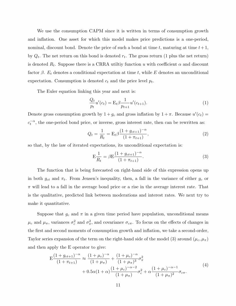
We use the consumption CAPM since it is written in terms of consumption growth

and inflation. One asset for which this model makes price predictions is a one-period,

nominal, discount bond. Denote the price of such a bond at time t, maturing at time t+1,

by Qt. The net return on this bond is denoted rt. The gross return (1 plus the net return)

is denoted Rt. Suppose there is a CRRA utiltiy function u with coefficient α and discount

factor β. Et denotes a conditional expectation at time t, while E denotes an unconditional

expectation. Consumption is denoted ct and the price level pt.

The Euler equation linking this year and next is:

Qt

ptu′(ct) = Etβ

1pt+1

u′(ct+1). (1)

Denote gross consumption growth by 1 + gc and gross inflation by 1 +π. Because u′(ct) =

c−αt , the one-period bond price, or inverse, gross interest rate, then can be rewritten as:

Qt =1Rt

= Etβ(1 + gct+1)−α

(1 + πt+1), (2)

so that, by the law of iterated expectations, its unconditional expectation is:

E1Rt

= βE(1 + gct+1)−α

(1 + πt+1). (3)

The function that is being forecasted on right-hand side of this expression opens up

in both gct and πt. From Jensen’s inequality, then, a fall in the variance of either gc or

π will lead to a fall in the average bond price or a rise in the average interest rate. That

is the qualitative, predicted link between moderations and interest rates. We next try to

make it quantitative.

Suppose that gc and π in a given time period have population, unconditional means

μc and μπ, variances σ2c and σ2

π, and covariance σcπ. To focus on the effects of changes in

the first and second moments of consumption growth and inflation, we take a second-order,

Taylor series expansion of the term on the right-hand side of the model (3) around (μc, μπ)

and then apply the E operator to give:

E(1 + gct+1)−α

(1 + πt+1)≈ (1 + μc)−α

(1 + μπ)+

(1 + μc)−α

(1 + μπ)3σ2

π

+ 0.5α(1 + α)(1 + μc)−α−2

(1 + μπ)σ2

c + α(1 + μc)−α−1

(1 + μπ)2σcπ.

(4)

11

The economic interpretation of this key equation is standard. High mean inflation, μπ

is associated with high average interest rates from the usual Fisher effect. Consumption

growth affects interest rates because of risk-adjusting bond prices and payoffs. Thus the

more rapid is consumption growth on average the less valuable is a future payoff from

holding the bond, so the lower is the bond price and the higher the return. And greater

volatility encourages precautionary saving, which leads to a higher bond price or a lower

return. Thus the theory links the mean bond price (or inverse of the gross return) to the

first and second moments of consumption growth and inflation. The theory also tells us

how to weight the means and variances of the two growth rates. And it tells us that shifts

in their covariance may be worth investigating as a source of shifts in average interest

rates.

We need values for the parameters α and β in order to predict the effect of moderations.

To estimate those values, we use the property that the moment condition (3) holds in each

time period. The underlying philosophy is that these sample moments would converge to

the population moments – which satisfy equation (3) exactly under the null hypothesis

that the model is accurate – if the sample from any given volatility regime became large

enough. Thus we estimate and test using the sample versions of this condition,

Ti∑t=1

[1Rt

− β(1 + gct+1)−α

1 + πt+1

]= 0, (5)

for each Ti. Estimation by GMM chooses parameter values to minimize the (weighted) sum

of squared deviations (residuals) from this equation. It thus uses unconditional moments.

To see that splitting the sample across the Ti identifies the parameters even though

we have only one moment condition (5), imagine substituting the sample version of the

approximation (4) into the estimating equations (5) (although estimate without using the

approximation). You can see that the equations in different time periods i are not identical

as long as at least one moment of consumption growth or inflation changes across regimes.

As long as there is at least one moderation, and so two distinct periods of time, we can

identify and estimate both parameters. If there is more than one moderation, then the

12

parameters are overidentified, because there are more time periods than parameters, which

provides the usual J-test.

5. Annual Evidence 1889-2006

The annual interest rate series again comes from the Shiller data set, updated by the

authors. Details are given in the appendix. Section 3 showed that there were two breaks

in the variances of gc and π, in 1946 and 1984. There is a break in the mean of inflation in

1984. Using the sample version of the unconditional asset-pricing model (3) in each of the

periods 1889-1945, 1946-1983, and 1984-2006 gives three moment conditions. With two

parameters to estimate, we then can use GMM and also test the model’s fit based on its

overidentification.

Estimation by iterated GMM in annual data gives the following coefficients, with

standard errors in parentheses: α = −0.943(3.19) and β = 0.963(0.057). The J-test

statistic, with 1 degree of freedom is 3.52, with a p-value of 0.06. Thus the restrictions

across the three time periods would narrowly be accepted at the traditional 5% significance

level. But the value of α is insignificantly different from zero. Because α cannot be

identified with any precision, we next set it equal to zero and re-estimate, finding that

β = 0.9807(0.0034) and J(2) = 4.40 with a p-value of 0.11.

These findings mean that the two moderations in consumption-growth volatility prob-

ably did not contribute to changes in average interest rates. With this part of our research

question answered, we can set α = 0 in the approximation (4) to give:

E1

(1 + πt+1)≈ 1

(1 + μπ)+

σ2π

(1 + μπ)3. (6)

so that the approximate asset-pricing model is:

E1Rt

≈ β

[1

(1 + μπ)+

σ2π

(1 + μπ)3

]. (7)

This result gives us a framework in which to investigate the likely impact on interest

rates (or, strictly speaking, average bond prices) of (a) the 1946 and 1984 moderations in

inflation and, later, (b) shifts in the mean of inflation associated with the 1969-1983 period.

13

This specialization of the asset-pricing model implicitly uses risk-neutrality, because α is

set at zero. But it still involves an ‘inflation risk premium’, in that a higher inflation

variance leads to a higher bond prices and lower interest rate.

Our evidence on α leads to the conclusion that changes in the moments of consumption

growth did not cause changes in average interest rates. The reader might wonder whether

using traditional instruments (like lagged variables) in GMM estimation would lead to

a precisely estimated, positive α. We argue that it would not, for there is a wealth of

relatively negative evidence on the CCAPM using this approach, as surveyed by Campbell,

Lo, and MacKinlay (1997) and Cochrane (2001). By using a new set of moments, we

provide new evidence on the CCAPM that reinforces the finding that it is difficult to find

an association between consumption growth and bond returns. Another way to make this

same point is that our specific GMM estimator is set up to identify α solely from the shifts

in unconditional moments across regimes. So finding that α is insignficantly different from

zero is indeed evidence that shifts in the moments of consumption were not related to

shifts in the average bond price or interest rate.

This finding does not mean that we require the real interest rate to be constant. It

could vary within each regime. Or, it could vary in moments across regimes but in a way

unrelated to the changes in the moments of consumption growth. The p-value for the

J-test is relatively low (and even lower below in quarterly data), which means that there

is variation in average bond prices or interest rates across time periods that is unrelated

to the variation in the moments of inflation. Hence our conclusions about the role of

inflation moments must be provisional, pending the identification of a better-fitting asset-

pricing model. However, we do know that such a model will not assign a central role to

consumption growth.

We construct and report predicted means – denoted m – using the sample version of

the inflation-based model (7):

mi(R−1) = β

[1

(1 + mi(π))+

sd2i (π)

(1 + mi(π))3

]. (8)

If we (a) ignored Jensen’s inequality and (b) approximated ln(1+ rt) by rt (which roughly

14

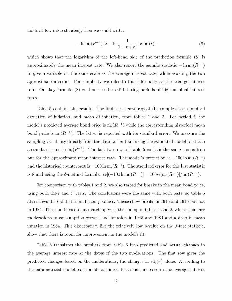
holds at low interest rates), then we could write:

− ln mi(R−1) ≈ − ln1

1 + mi(r)≈ mi(r), (9)

which shows that the logarithm of the left-hand side of the prediction formula (8) is

approximately the mean interest rate. We also report the sample statistic − ln mi(R−1)

to give a variable on the same scale as the average interest rate, while avoiding the two

approximation errors. For simplicity we refer to this informally as the average interest

rate. Our key formula (8) continues to be valid during periods of high nominal interest

rates.

Table 5 contains the results. The first three rows repeat the sample sizes, standard

deviation of inflation, and mean of inflation, from tables 1 and 2. For period i, the

model’s predicted average bond price is mi(R−1) while the corresponding historical mean

bond price is mi(R−1). The latter is reported with its standard error. We measure the

sampling variability directly from the data rather than using the estimated model to attach

a standard error to mi(R−1). The last two rows of table 5 contain the same comparison

but for the approximate mean interest rate. The model’s prediction is −100 ln mi(R−1)

and the historical counterpart is −100 ln mi(R−1). The standard error for this last statistic

is found using the δ-method formula: se[(−100 ln mi(R−1)] = 100se[mi(R−1)]/mi(R−1).

For comparison with tables 1 and 2, we also tested for breaks in the mean bond price,

using both the t and U tests. The conclusions were the same with both tests, so table 5

also shows the t-statistics and their p-values. These show breaks in 1915 and 1945 but not

in 1984. These findings do not match up with the timing in tables 1 and 2, where there are

moderations in consumption growth and inflation in 1945 and 1984 and a drop in mean

inflation in 1984. This discrepancy, like the relatively low p-value on the J-test statistic,

show that there is room for improvement in the model’s fit.

Table 6 translates the numbers from table 5 into predicted and actual changes in

the average interest rate at the dates of the two moderations. The first row gives the

predicted changes based on the moderations, the changes in sdi(π) alone. According to

the parametrized model, each moderation led to a small increase in the average interest

15

rate. The next row gives the predicted changes based on changes in average inflation,

mi(π), alone. Here the theory predicts a much larger effect. The third row gives the

combined effect (the effects are not exactly additive but close to that in practice) while

the fourth row gives the actual change. For 1946 the model’s predicted change is on the

same scale as the actual change, and most of the predicted change stems from the change

in actual inflation.

As for the 1984 moderation, here the theory predicts a fall in the mean interest rate,

whereas the actual rate rose. In this case, it is the contribution of the moderation (which

leads to a small increase in the interest rate) that is comparable in scale to the actual

change. Again this predicted effect is much smaller than the predicted effect of the change

in mean inflation. We re-examine these findings with quarterly data in the next section.

6. Quarterly Evidence 1947-2006

In the annual-data exercise we did not separate the Great Inflation, due to the limited

number of observations. With 15 annual observations the moments from the 1969-1983

period have large standard errors. Turning to quarterly, postwar data allows us to isolate

that period yet draw more reliable inferences. And the greater number of observations also

allows us to estimate the parameters solely in postwar data.

The three time periods are 1947:1-1968:4, 1969:1-1983:4, and 1984:1-2006:3. The

interest rate applies to a 3-month T-bill. The interest rate and the growth rates are annu-

alized, so the results are directly comparable to those of the previous section. The same

GMM estimator yields these parameters estimates, with standard errors in parentheses:

α = −1.95(19.7) and β = 0.9496(0.357). The J-statistic is 6.61 with a p-value of 0.01.

Hence the stability of the pricing model across the three time periods is rejected at the 1%

significance level.

When we examine estimation using different combinations of the three time periods,

we find that α is estimated imprecisely in all cases. Thus the rejection under the J-test

stems from small, but significant changes in β across these periods. But since the level of β

does not affect the model’s prediction for changes in the mean interest rate at moderations,

16

we proceed to document the predictions. And since we find no significant α we use the

same approximation formula (7) based on the mean and variance of the inflation rate.

When we re-estimate with α set at 0 we find β = 0.9889(0.002), so we use this value to

find the predicted average bond prices and (roughly) interest rates in each time period.

Tables 7 contains the results. Again we report the t-test statistic and its p-value for

the test of a break in the average bond price between periods. This test reveals significant

breaks (with p-values of 0.00) at both 1969 and 1984. In the macroeconomic quantities,

tables 3 and 4 showed breaks at both dates in two variables: the standard deviation of

consumption growth and the mean inflation rate. In this dataset, then, the timing of

breaks seems to be aligned between bond prices and fundamentals. However, if the break

in σc were driving the break in the mean bond price, that would lead to a role for α in

the pricing equation, since it is differences in unconditional means that the estimator tries

to match. Since we do not find a significant positive α, it seems more likely that the two

breaks in average bond prices were driven by breaks in the moments of inflation.

Table 8 shows predicted and actual changes between periods in the approximate mean

interest rate. This time both predicted interest-rate changes are on the same scale as the

actual changes, though the theory under-predicts the rise in 1969 and over-predicts the fall

in 1984. A key virtue of the theory is that it describes the joint effects of both means and

variances on the interest rate. Once again one can see that the lion’s share of explanation

is done by mi(π), while the 1984 moderation – the drop in sdi(π) – affects only the second

decimal place of the interest rate. Thus we find that that the theory predicts relatively

modest effects of the Great Moderation. Instead, changes in average inflation seem more

likely to explain most of the changes in average interest rates, through the traditional

Fisher effect.

In postwar quarterly data we also studied interest rates at 1-year maturity. The data

appendix provides details of two different interest rate series we adopted. One of these, the

quarterly average of the 1-year treasury constant-maturity rate, begins in 1953. Making

a virtue of necessity, this sample thus begins after the 1951 Treasury-Federal Reserve

Accord that released the Federal Reserve from any obligation to support the price of

17

federal government debt. We aligned these interest rates with the corresponding year-to-

year growth rates in quarterly consumption and prices.

The conclusions from these data are the same as those documented in the tables.

Year-to-year growth rates of output, consumption, and prices are moderated after 1983.

Average inflation is significantly higher during 1969-1983 than before or after. In the asset-

pricing model we cannot reject the hypothesis that α = 0 at traditional significance levels.

With one interest rate series α is negative and with the other it is positive. And, changes

in mean inflation drive most of the changes in predicted, average nominal interest rates.

Finally, note that the finding that changes in the mean of the inflation rate mattered

more than changes in the variance is in no way rigged into the setup of the central equation

(7) used to find the predictions. Inspection of this equation shows that large changes in

the variance will lead to large changes in bond prices and interest rates, especially if the

mean inflation rate is small. Historically, the changes in variance simply were not large

enough (nor the mean small enough) for this to have happened.

7. Habit Persistence?

A variety of contributions in asset-pricing and macroeconomics have worked with

preferences different from the ones we have adopted so far. Perhaps the most widely used

revision uses a utility function in which individual consumption is assessed by comparison

to aggregate consumption or to past consumption, a reference level sometimes referred to

as ‘habit.’ Abel (1990) called this feature of utility ‘catching up with the Joneses.’ This

theory has been promising in helping economists understand a range of features of asset

prices, such as the equity premium. But we next show that attributing these preferences

to savers does not affect our results about moderations and interest rates.

The measure of habit can be current, lagged, or a mixture, and can scale consumption

by subtraction or multiplication We first use Abel’s (1999) version, which measures habit

as a mixture of current and lagged consumption and enters it multiplicatively into the

utility function. The utility function in a given time period now is:

u =1

1 − α

(ct

st

)1−α

, (10)

18

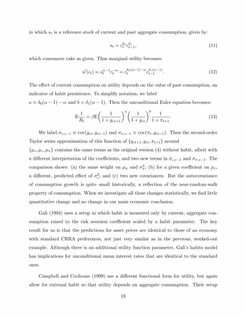
in which st is a reference stock of current and past aggregate consumption, given by:

st = cδ0t cδ1

t−1, (11)

which consumers take as given. Thus marginal utility becomes:

u′(ct) = sα−1t c−α

t = cδ0(α−1)−αt c

δ1(α−1)t−1 . (12)

The effect of current consumption on utility depends on the value of past consumption, an

indicator of habit persistence. To simplify notation, we label

a ≡ δ0(α − 1) − α and b = δ1(α − 1). Then the unconditional Euler equation becomes:

E1Rt

= βE(

11 + gct+1

)a(1

1 + gct

)b 11 + πt+1

. (13)

We label σc,c−1 ≡ cov(gct, gct−1) and σπ,c−1 ≡ cov(πt, gct−1). Then the second-order

Taylor series approximation of this function of {gct+1, gct, πt+1} around

{μc, μc, μπ} contains the same terms as the original version (4) without habit, albeit with

a different interpretation of the coefficients, and two new terms in σc,c−1 and σπ,c−1. The

comparison shows: (a) the same weight on μπ and σ2π; (b) for a given coefficient on μc,

a different, predicted effect of σ2c ; and (c) two new covariances. But the autocovariance

of consumption growth is quite small historically, a reflection of the near-random-walk

property of consumption. When we investigate all these changes statistically, we find little

quantitative change and no change in our main economic conclusion.

Gali (1994) uses a setup in which habit is measured only by current, aggregate con-

sumption raised to the risk aversion coefficient scaled by a habit parameter. The key

result for us is that the predictions for asset prices are identical to those of an economy

with standard CRRA preferences, not just very similar as in the previous, worked-out

example. Although there is an additional utility function parameter, Gali’s habits model

has implications for unconditional mean interest rates that are identical to the standard

ones.

Campbell and Cochrane (1999) use a different functional form for utility, but again

allow for external habit so that utility depends on aggregate consumption. Their setup

19

has success in matching asset-pricing features such as the equity premium and a range of

cyclical features of stock prices. They observe that models with external habit and random-

walk consumption sometimes lead to large swings in the risk-free interest rate. However,

their model is parametrized to have a constant, real interest rate (p 213, equation 12) ,

given by − lnβ + αμc − 0.5α(1 − φ), in which φ is the coefficient in an AR(1) process

for the stock of external habit. This takes the form we have already considered, with the

exception of the new, last term. They use both a long span of annual data and postwar

quarterly data to calibrate their model, and adopt φ = 0.87. It is possible that this varies

over different time periods, and this would be worth studying. However, great moderations

are not described in terms of changes in the persistence properties of the reference level of

consumption, which is a feature of preferences.

These examples take the reference level of consumption as given, and so are sometimes

referred to as embodying ‘external habit.’ Another possibility is ‘internal habit’ in which

the consumer takes into account the impact of the current consumption choice on the stock

of habit and hence future utility. In this case the asset prices depend on the expected value

of future consumption growth xt+1, in addition to xt and xt−1. But since the unconditional

mean of each of these terms is the same (and consumption growth has little autocorrelation)

the predictions for average interest rates do not change significantly. We omit the details,

but again this modification would not affect our findings.

There are many other examples of ‘exotic’ preferences, featuring a discount factor

that depends on the level of consumption, quasi-geometric discounting, or disappointment

aversion. Backus, Routledge, and Zin (2004) provide a complete survey. For adopting

one of these utility models to change our findings, one would need to find (a) changes

in the predictions for unconditional mean interest rates on bonds that (b) are driven by

a macroeconomic statistic that shifts during GMs. We have not come across examples

that satisfy these requirements, but studying the observable implications of these utility

functions is an active research area.

8. Conclusions

The US Geat Moderation of the 1980s is an ideal episode with which to study our

20

understanding of interest-rate history. Its timing has been studied extensively, it seems

to have been a sharp break, and it was accompanied by a shift in the inflation process.

We combine this perspective with a long span of data that includes the comparable 1946

moderations in both real consumption growth and inflation. Asset-pricing theory, along

with assumptions about the utility function, links average, nominal interest rates simulta-

neously to both the means and variances of consumption growth and inflation. Because

we base predictions on unconditional moments, our findings apply whether these moder-

ations were due to decreases in unconditional variances or to decreases in persistence. A

central finding is that shifts in twentieth-century US interest rates probably were due to

a traditional source – the average level of inflation – rather than to shifts in the volatility

of consumption growth or inflation.

The p-values of tests of overidentification (based on the stability of the asset-pricing

model) are low both for the long span of annual data and for the postwar quarterly data.

That finding gives gives scope for further study of moderations and U.S. interest rates. But

moderations in consumption growth do not seem to be the source of changes in average

interest rates. There also is scope for further study using moderations in other countries,

though we have not pursued that because there is so far less consensus about the timing

than in the US case. And moderations in output in other countries did not generally

coincide with moderations in inflation, which makes it difficult to use long spans of data.

It also would be interesting to study evidence of moderation in household consumption,

even though long time spans of disaggregated consumption data may not be available.

Our use of unconditional moments is appropriate whether the GM was due to a change

in conditional variance or in persistence. But other properties of asset prices (such as the

shape of the term structure of interest rates) may be sensitive to this distinction and so

provide evidence on these two separate changes. Finally, we have taken the moderations

as given and focused on their effects. It would of course be interesting to compare the

causes of the 1984 moderation with those of the 1946 one.

21

Appendix: Data Sources and Definitions

Annual Data: Real output per capita, y, is from Johnston and Williamson (2007). Real

consumption of nondurables and services per capita, c, and the deflator for personal con-

sumption expenditures, p, are from www.econ.yale.edu/∼shiller/dat/chapt26. xls

which is described by Shiller (1989) and revised and updated by us. The interest rate, r, is

a synthetic series constructed from 6-month rates, denoted r6 using the following formula:

r = 100[

1(1 − r6(January)/200)(1 − r6(July)/200)

− 1],

as described and adopted by Shiller (1989, p 444). For 1889-2004 the underlying series

comes from the Shiller data set. Data prior to 1939 are 4-6-month commercial paper rates

from Macaulay (1938). For 1939 to 1997 the interest rate is the 6-month commercial paper

rate from the Federal Reserve Bulletin; for 1998-2004, it is the rate on 6-month certificates

of deposit on the secondary market, from the Federal Reserve; for 2005 and 2006 we update

the series with the 6-month certificate of deposit rate.

Quarterly Data: Output, y, is real per capita chained GDP; consumption, c, is real, per

capita consumption of nondurables and services (NDS); the price level is the associated

deflator. Chained NDS expenditures are computed with a Fisher ideal chain index. All

data are seasonally adjusted at annual rates. The source of the NIPA data is the Bureau

of Economic Analysis via the FRED database at the Federal Reserve Bank of St. Louis.

The population measure is found at www.bea.gov, NIPA Table 7.1. The interest rate, r,

is the three-month T-bill rate, from FRED series tb3m, averaged from monthly data.

In the postwar data we also studied quarterly observations on 1-year interest rates. The two

alternative ways of measuring this rate were: (a) the synthetic 1-year rate, for 1947:1-1964:2

from the 4 to 6-month commercial paper rate from January Federal Reserve Bulletins

1948-1965; for 1964:2-2006:4 6-month certificate of deposit rate from FRED and the Federal

Reserve; and (b) the 1-year treasury constant-maturity rate, quarterly average 1953:2-

2006:4, from the Board of Governors of the Federal Reserve System H.15 Selected Interest

Rates.

22

References

Abel, Andrew (1990) Asset prices under habit formation and catching up with the Joneses.American Economic Review (P) 80, 43-47.

Abel, Andrew (1999) Risk premia and term premia in general equilibrium. Journal ofMonetary Economics 43, 3-33.

Armesto, Michelle T. and Jeremy M. Piger (2005) International perspectives on the ”GreatModeration”. Federal Reserve Bank of St. Louis, International Economic Trends

Ahmed, Shaghil, Andrew Levin, and Beth Anne Wilson (2002) Recent U.S. macroeconomicstability: Good policies, good practices, or good luck? Board of Governors of theFederal Reserve System, International Finance Discussion Paper 2002-730.

Backus, David K., Bryan Routledge, and Stanley Zin (2004) Exotic preferences for macroe-conomists. NBER Macroeconomic Annual. MIT Press: Cambridge, MA.

Balke, Nathan S. and Robert J. Gordon (1989) The estimation of prewar Gross nationalproduct: methodology and new evidence. Journal of Political Economy 97, 38-92.

Benati, Luca (2007) The ‘Great Moderation’ in the United Kingdom. forthcoming in theJournal of Money, Credit and Banking

Benati, Luca and Paolo Surico (2007) VAR analysis and the Great Moderation. Bank ofEngland, External MPC Discussion Paper no. 18.

Bernanke, Ben S. (2004) The Great Moderation. Remarks at the meetings of the EasternEconomic Association, Washington, DC; February 20, 2004

Blanchard, Olivier, and John Simon (2001) The long and large decline in U.S. outputvolatility, Brookings Papers on Economic Activity, 1, pp. 135-64.

Blanchard, Olivier and Jordi Gali (2007) The macroeconomic effects of oil price shocks:Why are the 2000s so different from the 1970s? NBER working paper 13368.

Campbell, John Y. and John Cochrane (1999) By force of habit: A consumption-basedexplanation of aggregate stock market behavior. Journal of Political Economy 107,205-251.

Campbell, John Y., Andrew W. Lo, and A. Craig MacKinlay (1997) The Econometrics ofFinancial Markets. Princeton University Press: Princeton, NJ.

Campbell, Sean D. (2005) Stock market volatility and the Great Moderation. Financeand Economics Discussion Series 2005-47. Washington: Board of Governors of theFederal Reserve System, 2005.

Campbell, Sean D. (2007) Macroeconomic volatility, predictability and uncertainty in the”Great Moderation”: evidence from the survey of professional forecasters. Journalof Business and Economic Statistics 25, 191-200.

Cecchetti, Stephen G., Alfonso Flores-Launes, and Stefan Krause (2006) Assessing thesources of changes in the volatility of real growth. NBER working paper 11946.

Cecchetti, Stephen G., Peter Hooper, Bruce C. Kasman, Kermit L. Schoeholtz, and MarkW. Watson (2007) Understanding the evolving inflation process. U.S. MonetaryPolicy Forum 2007.http://research.chicagogsb.edu/igm/docs/2007USMPF-Report.pdf

Cochrane, John H. (2001) Asset Pricing. Princeton University Press.

Cogley, Timothy and Thomas J. Sargent (2001) Evolving post-world war II U.S. inflationdynamics. In NBER Macroeconomics Annual 2001, Bernanke B (ed.). MIT Press:Cambridge, MA.

Conover, W.J. (1999) Practical Nonparametric Statistics. 3rd. ed. John Wiley and Sons.

Fogli, Alessandra and Fabrizio Perri (2006) The “Great Moderation” and the US externalimbalance. NBER working paper no. 12708.

Gali, Jordi (1994) Keeping up with the Joneses: Consumption externalities, portfoliochoice, and asset prices. Journal of Money Credit and Banking 26, 1-8.

Johnston, Louis D. and Samuel H. Williamson (2007) What was the U.S. GDP then?MeasuringWorth.com

JP Morgan Chase (2007) Understanding the common evolution of global inflation. Eco-nomic Research Note, March 9.

Kahn, James, Margaret McConnell, and Gabriel Perez-Quiros (2002). On the causes of theincreased stability of the U.S. economy, Federal Reserve Bank of New York, EconomicPolicy Review, 8, pp. 183-202.

Kim, Chang-Jin and Charles Nelson (1999) Has the US economy become more stable?Review of Economics and Statistics 81, 608-616.

Macaulay, Frederick R. (1938) Some Theoretical Problems Suggested by the Movements ofInterest Rates, Bond Yields, and Stock Prices in the United States Since 1856. NewYork: NBER.

McConnell, Margaret M. and Gabriel Perez-Quiros (2000) Output fluctuations in theUnited States: What has changed since the early 1980s? American Economic Review90, 1464-1476.

Nason, James M. (2006) Instability in U.S. inflation: 1967-2005. Federal Reserve Bank ofAtlanta Economic Review 91(Q2), 39-59.

Officer, Lawrence H. (2007) The annual consumer price index for the United States, 1774-2006. MeasuringWorth.com

Romer, Christina D. (1986) Is the stabilization of the postwar economy a figment of thedata? American Economic Review 76, 314-334.

Romer, Christina (1999) Changes in business cycles: Evidence and explanations. Journalof Economic Perspectives 13(2), 23-44.

Rudebusch, Glenn D. and Tao Wu (2007) Accounting for a shift in term structure behaviorwith no-arbitrage and macro-finance models. Journal of Money, Credit, and Banking39, 395-422.

Sargent, Thomas J., Noah Williams, and Tao Zha (2006) Shocks and government beliefs:The rise and fall of American inflation. American Economic Review 96, 1193-1224.

Shiller, Robert J. (1989) Market Volatility. MIT Press.

Sims, Christopher and Tao Zha (2006) Were there regime shifts in US monetary policy?American Economic Review 96, 54-81.

Sprent, Peter and N.C. Smeeton (2001) Applied Nonparametric Statistical Methods. 3rd.ed. Boca Raton: Chapman and Hall.

Stock, James, and Mark Watson (2003) Has the business cycle changed? Evidence andexplanations. Federal Reserve Bank of Kansas City symposium, ”Monetary Policyand Uncertainty,” Jackson Hole, Wyoming, August 28-30.

Summers, Peter M. (2005) What caused the Great Moderation: Some cross-country Evi-dence. Federal Reserve Bank of Kansas City Economic Review, Third Quarter, 5-32.

Taylor, John B. (1999) A historical analysis of monetary policy rules. chapter 7 in Taylor,ed. Monetary Policy Rules. NBER/University of Chicago Press.

Weir, David R. (1986) The reliability of historical macroeconomic data for comparingcyclical stability. Journal of Economic History 46, 353-365.

Figure 1: Annual US Growth Rates and Interest Rates

Year

1900 1920 1940 1960 1980 2000

GD

P an

d C

onsu

mpt

ion

Gro

wth

(%)

-15

-10

-5

0

5

10

15

Year

1900 1920 1940 1960 1980 2000

Infla

tion

and

Inte

rest

Rat

es (%

)

-10

0

10

20

GDP growth

consumption growth

inflation rate

interest rate

Figure 2: Quarterly US Growth Rates and Interest Rates

Year

1950 1960 1970 1980 1990 2000

GD

P an

d C

onsu

mpt

ion

Gro

wth

(%)

-10

-5

0

5

10

15

Year

1950 1960 1970 1980 1990 2000

Infla

tion

and

Inte

rest

Rat

es (%

)

0

5

10

15

GDP growth

consumption growth

inflation rate

interest rate

Table 1: Great ModerationsAnnual GDP Growth, Consumption Growth, and Inflation

Variable 1889-1914 1915-1945 1946-1983 1984-2006

Ti 25 31 38 23

sdi(gy) 5.78 7.57 3.58 1.50

se[sdi(gy)] 0.83 0.98 0.42 0.23

Fy/(p) 0.58/(0.92) 4.46/(0.00) 5.75/(0.00)

sdi(gc) 4.93 4.61 2.00 0.88

se[sdi(gc)] 0.71 0.59 0.23 0.13

Fc/(p) 1.14/(0.36) 5.31/(0.00) 5.16/(0.00)

sdi(π) 2.88 7.78 3.36 0.93

se[sdi(π)] 0.42 1.00 0.39 0.14

Fπ/(p) 0.14/(0.99) 5.33/(0.00) 13.2/(0.00)

Notes: Ti is the number of observations in period i; gy is the percentagegrowth rate of real GDP per capita, gc is the percentage growth rate of realconsumption of nondurables and services per capita, π is the inflation rate inthe consumption deflator; sd is a standard deviation and se the associatedstandard error; F is the test statistic for equality of standard deviationsbetween the current and previous periods and p is the associated p-value.

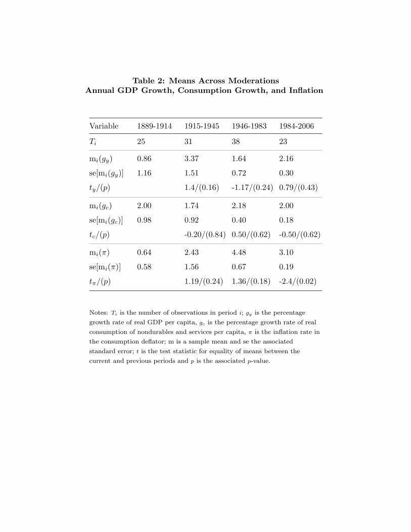
Table 2: Means Across ModerationsAnnual GDP Growth, Consumption Growth, and Inflation

Variable 1889-1914 1915-1945 1946-1983 1984-2006

Ti 25 31 38 23

mi(gy) 0.86 3.37 1.64 2.16

se[mi(gy)] 1.16 1.51 0.72 0.30

ty/(p) 1.4/(0.16) -1.17/(0.24) 0.79/(0.43)

mi(gc) 2.00 1.74 2.18 2.00

se[mi(gc)] 0.98 0.92 0.40 0.18

tc/(p) -0.20/(0.84) 0.50/(0.62) -0.50/(0.62)

mi(π) 0.64 2.43 4.48 3.10

se[mi(π)] 0.58 1.56 0.67 0.19

tπ/(p) 1.19/(0.24) 1.36/(0.18) -2.4/(0.02)

Notes: Ti is the number of observations in period i; gy is the percentagegrowth rate of real GDP per capita, gc is the percentage growth rate of realconsumption of nondurables and services per capita, π is the inflation rate inthe consumption deflator; m is a sample mean and se the associatedstandard error; t is the test statistic for equality of means between thecurrent and previous periods and p is the associated p-value.

Table 3: Postwar Great ModerationsQuarterly GDP Growth, Consumption Growth, and Inflation

Variable 1947:1-1968:4 1969:1-1983:4 1984:1-2006:3

Ti 87 60 91

sdi(gy) 4.84 4.70 2.08

se[sdi(gy)] 0.37 0.43 0.15

Fy/(p) 1.06/(0.40) 5.13/(0.00)

sdi(gc) 2.73 2.13 1.32

se[sdi(gc)] 0.21 0.20 0.10

Fc/(p) 1.65/(0.02) 2.58/(0.00)

sdi(π) 2.46 2.60 1.26

se[sdi(π)] 0.19 0.24 0.09

Fπ/(p) 0.89/(0.68) 4.25/(0.00)

Notes: Ti is the number of observations in period i; gy is the percentage growth rateof real GDP per capita, gc is the percentage growth rate of real consumption ofnondurables and services per capita, π is the inflation rate in the consumptiondeflator (all at annual rates); sd is a standard deviation and se the associatedstandard error; F is the test statistic for equality of standard deviations betweenthe current and previous periods and p is the associated p-value.

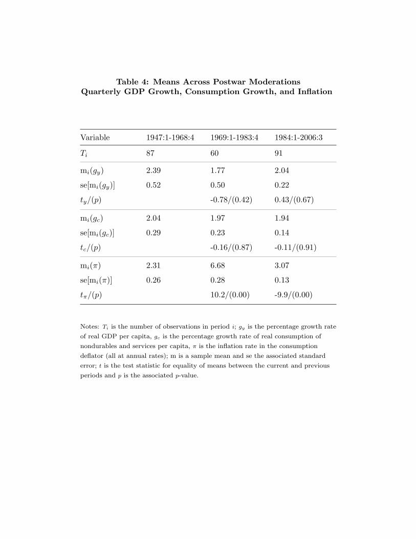
Table 4: Means Across Postwar ModerationsQuarterly GDP Growth, Consumption Growth, and Inflation

Variable 1947:1-1968:4 1969:1-1983:4 1984:1-2006:3

Ti 87 60 91

mi(gy) 2.39 1.77 2.04

se[mi(gy)] 0.52 0.50 0.22

ty/(p) -0.78/(0.42) 0.43/(0.67)

mi(gc) 2.04 1.97 1.94

se[mi(gc)] 0.29 0.23 0.14

tc/(p) -0.16/(0.87) -0.11/(0.91)

mi(π) 2.31 6.68 3.07

se[mi(π)] 0.26 0.28 0.13

tπ/(p) 10.2/(0.00) -9.9/(0.00)

Notes: Ti is the number of observations in period i; gy is the percentage growth rateof real GDP per capita, gc is the percentage growth rate of real consumption ofnondurables and services per capita, π is the inflation rate in the consumptiondeflator (all at annual rates); m is a sample mean and se the associated standarderror; t is the test statistic for equality of means between the current and previousperiods and p is the associated p-value.

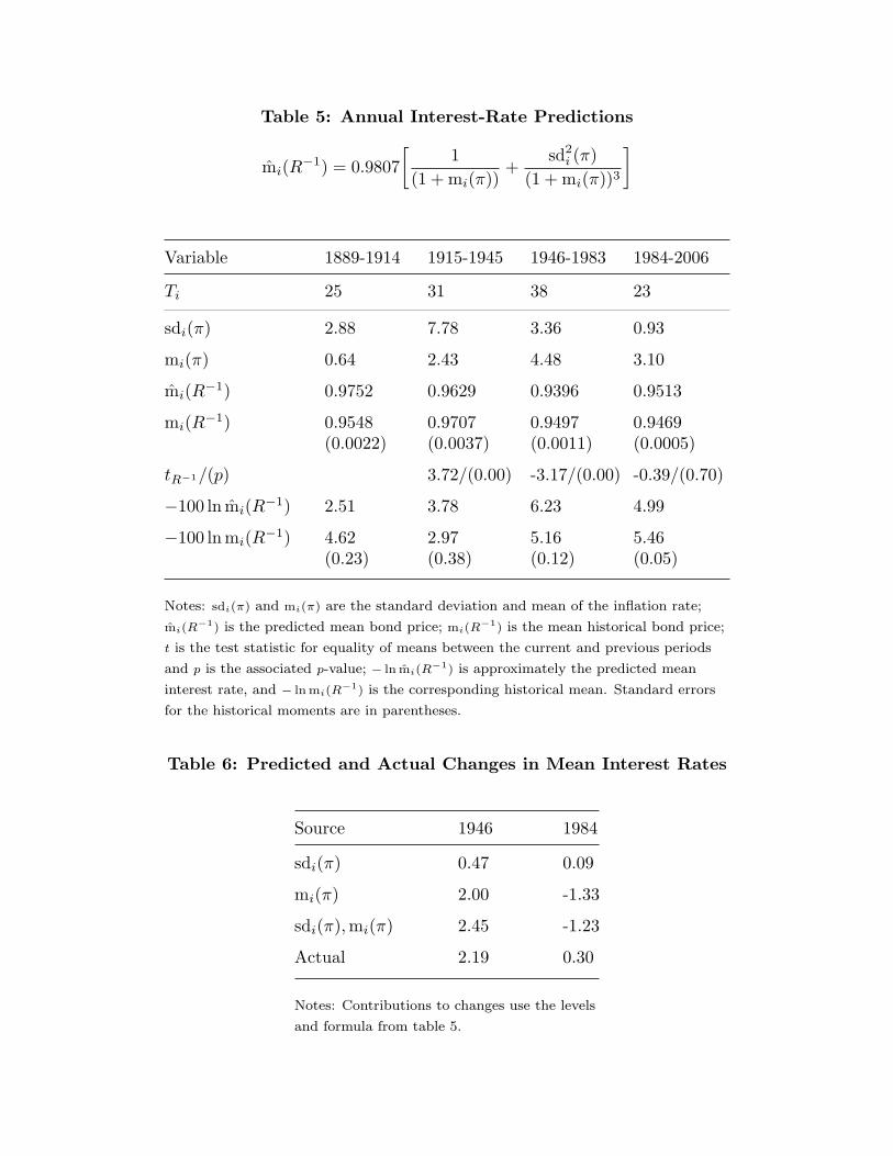
Table 5: Annual Interest-Rate Predictions

mi(R−1) = 0.9807[

1(1 + mi(π))

+sd2

i (π)(1 + mi(π))3

]

Variable 1889-1914 1915-1945 1946-1983 1984-2006

Ti 25 31 38 23

sdi(π) 2.88 7.78 3.36 0.93

mi(π) 0.64 2.43 4.48 3.10

mi(R−1) 0.9752 0.9629 0.9396 0.9513

mi(R−1) 0.9548 0.9707 0.9497 0.9469(0.0022) (0.0037) (0.0011) (0.0005)

tR−1/(p) 3.72/(0.00) -3.17/(0.00) -0.39/(0.70)

−100 ln mi(R−1) 2.51 3.78 6.23 4.99

−100 ln mi(R−1) 4.62 2.97 5.16 5.46(0.23) (0.38) (0.12) (0.05)

Notes: sdi(π) and mi(π) are the standard deviation and mean of the inflation rate;mi(R−1) is the predicted mean bond price; mi(R−1) is the mean historical bond price;t is the test statistic for equality of means between the current and previous periodsand p is the associated p-value; − ln mi(R−1) is approximately the predicted meaninterest rate, and − ln mi(R−1) is the corresponding historical mean. Standard errorsfor the historical moments are in parentheses.

Table 6: Predicted and Actual Changes in Mean Interest Rates

Source 1946 1984

sdi(π) 0.47 0.09

mi(π) 2.00 -1.33

sdi(π),mi(π) 2.45 -1.23

Actual 2.19 0.30

Notes: Contributions to changes use the levelsand formula from table 5.

Table 7: Quarterly Interest-Rate Predictions

mi(R−1) = 0.9889[

1(1 + mi(π))

+sd2

i (π)(1 + mi(π))3

]

Variable 1947:1-1968:4 1969:1-1983:4 1984:1-2006:3

Ti 87 60 91

sdi(π) 2.46 2.60 1.26

mi(π) 2.31 6.68 3.07

mi(R−1) 0.9671 0.9275 0.9596

mi(R−1) 0.9751 0.9299 0.9535(0.0013) (0.0032) (0.0021)

tR−1/(p) -13.03/(0.00) 6.17/(0.00)

−100 ln mi(R−1) 3.34 7.52 4.12

−100 ln mi(R−1) 2.52 7.27 4.76(0.13) (0.34) (0.22)

Notes: sdi(π) and mi(π) are the standard deviation and mean of the inflation rate; mi(R−1)

is the predicted mean bond price; mi(R−1) is the historical mean bond price; t is the teststatistic for equality of means between the current and previous periods and p is theassociated p-value; − ln mi(R−1) is approximately the predicted mean interest rate, and− ln mi(R−1) is the corresponding historical mean. Standard errors for the historicalmoments are in parentheses.

Table 8: Predicted and Actual Changes in Mean Interest Rates

Source 1969 1984

sdi(π) -0.01 0.05

mi(π) 4.19 -3.45

sdi(π),mi(π) 4.18 -3.40

Actual 4.75 -2.51

Notes: Contributions to changes use the levelsfrom table 7.