Graduate School ETD Form 9

Graduate School ETD Form 9 (Revised 12/07)

PURDUE UNIVERSITY GRADUATE SCHOOL

Thesis/Dissertation Acceptance

This is to certify that the thesis/dissertation prepared

By

Entitled

For the degree of

Is approved by the final examining committee:

Chair

To the best of my knowledge and as understood by the student in the Research Integrity and Copyright Disclaimer (Graduate School Form 20), this thesis/dissertation adheres to the provisions of Purdue University’s “Policy on Integrity in Research” and the use of copyrighted material.

Approved by Major Professor(s): ____________________________________

____________________________________

Approved by: Head of the Graduate Program Date

Tarek M. Elharis

A Multi-step Reaction Model for Stratified-Charge Combustion in Wave Rotors

Master of Science in Mechanical Engineering

M. Razi Nalim

Likun Zhu

Tamer Wasfy

M. Razi Nalim

M. Razi Nalim 04/26/2011

Graduate School Form 20 (Revised 9/10)

PURDUE UNIVERSITY GRADUATE SCHOOL

Research Integrity and Copyright Disclaimer

Title of Thesis/Dissertation:

For the degree of Choose your degree

I certify that in the preparation of this thesis, I have observed the provisions of Purdue University Executive Memorandum No. C-22, September 6, 1991, Policy on Integrity in Research.*

Further, I certify that this work is free of plagiarism and all materials appearing in this thesis/dissertation have been properly quoted and attributed.

I certify that all copyrighted material incorporated into this thesis/dissertation is in compliance with the United States’ copyright law and that I have received written permission from the copyright owners for my use of their work, which is beyond the scope of the law. I agree to indemnify and save harmless Purdue University from any and all claims that may be asserted or that may arise from any copyright violation.

______________________________________ Printed Name and Signature of Candidate

______________________________________ Date (month/day/year)

*Located at http://www.purdue.edu/policies/pages/teach_res_outreach/c_22.html

A Multi-step Reaction Model for Stratified-Charge Combustion in Wave Rotors


Tarek M. Elharis

04/11/2011

A MULTI-STEP REACTION MODEL FOR

STRATIFIED-CHARGE COMBUSTION IN WAVE ROTORS

A Thesis

Submitted to the Faculty

of

Purdue University

by

Tarek M. Elharis

In Partial Fulfillment of the

Requirements for the Degree

of


May 2011

Purdue University

Indianapolis, Indiana

ii

ACKNOWLEDGMENTS

This thesis would not have been completed without the help and guidance of

several individuals who shared their valuable time and knowledge, and contributed in

different ways towards this work.

The author would like to express his utmost gratitude to Dr. Razi Nalim, the chair

of the committee, for his guidance and encouragement during the entire research work.

Dr. Nalim shared his knowledge and experience that will always be appreciated.

Also the author would like to thank his advisory committee members, Dr. Likun

Zhu and Dr. Tamer Wasfy, for their perceptive assistance during the completion of this

thesis.

Financial support for this work from Rolls-Royce North American Technologies

Inc., LibertyWorks, and the valuable insights from Dr. Philip Snyder and other personnel

are acknowledged.

Thanks to Rob Meagher and Don Krawjeski of computer network center for their

valuable time and support. Recognition goes to my colleagues of combustion and

propulsion research lab for their continuous assistance and provision.

iii

TABLE OF CONTENTS

Page

LIST OF TABLES ...............................................................................................................v

LIST OF FIGURES ........................................................................................................... vi

NOMENCLATURE .......................................................................................................... ix

1. INTRODUCTION ..........................................................................................................1 1.1. Background ..............................................................................................................1 1.2. Previous Work ..........................................................................................................6

1.3. Problem Statement ...................................................................................................7

1.4. Objectives .................................................................................................................8

2. NUMERICAL MODEL ..................................................................................................9 2.1. Governing Equations ................................................................................................9

2.2. Viscous Effects (Friction) ......................................................................................11 2.3. Heat Transfer ..........................................................................................................11 2.4. Turbulence Eddy-Diffusivity Model ......................................................................13

2.5. Developed Combustion Model...............................................................................13

2.6. Leakage Model .......................................................................................................20

2.7. Non-dimensionalization .........................................................................................23

2.8. Summary ................................................................................................................25

3. NUMERICAL SCHEME ..............................................................................................27 3.1. TVD Lax-Wendroff Scheme ..................................................................................27

3.2. The Jacobian of the Flux Vector ............................................................................28

3.3. Eigenvalues and Eigenvectors ................................................................................29

4. WAVE-ROTOR CONSTANT-VOLUME COMBUSTOR .........................................30 4.1. Rig Description ......................................................................................................31 4.2. WRCVC Operation procedure ...............................................................................33

4.3. WRCVC Instrumentations .....................................................................................33

4.4. Adapting Friction Factor for WRCVC Rig ............................................................35

5. SIMULATIONS AND COMPARISONS ....................................................................39 5.1. Test Case A ............................................................................................................43 5.2. Test Case B.............................................................................................................56

5.3. Test Case C.............................................................................................................64

5.4. Test Case D ............................................................................................................70

iv

Page

6. CONCLUSIONS AND RECOMMENDATIONS .......................................................73

6.1. Conclusions ............................................................................................................73

6.2. Recommendations ..................................................................................................74

LIST OF REFERENCES ...................................................................................................75

APPENDICES

Appendix A Viscous Friction .......................................................................................79 Appendix B Heat Transfer ............................................................................................82 Appendix C Turbulence Eddy-Diffusivity ...................................................................84 Appendix D Boundary Conditions ...............................................................................86

Appendix E TVD Lax-Wendroff Scheme ....................................................................87 Appendix F Approximate Riemann Solvers (The Method of Roe)..............................90

Appendix G Wave Strengths ........................................................................................91

v

LIST OF TABLES

Table Page

Table 2.1 Molecular Weight of Species ......................................................................... 16

Table 2.2 Species internal energy of formation at 1450 K ............................................ 18

Table 2.3 Turbulent Parameters ..................................................................................... 19

Table 4.1 Details of WRCVC rig dimensions ............................................................... 31

Table 4.2 Comparison between WRCVC rig and NASA phase I rig ............................ 37

Table 5.1 Summary of Test cases presented .................................................................. 40

Table 5.2 Boundary conditions of simulation of case A ................................................ 47

Table 5.3 User defined parameters ................................................................................ 47

Table 5.3 Boundary conditions of simulation of case C ................................................ 65

vi

LIST OF FIGURES

Figure Page

Figure 1.1 Comparison between Humphrey cycle and Brayton cycle ............................. 2

Figure 1.2 Exploded view of WRCVC schematic ........................................................... 3

Figure 1.3 Developed view (unrolled) of WRCVC ......................................................... 4

Figure 2.1 A schematic diagram for heat transfer path in a passage ............................. 12

Figure 2.2 Leakage paths from a representing passage of WRCVC ............................. 21

Figure 2.3 A schematic representation for leakage flow through the gap ..................... 21

Figure 4.1 WRCVC test rig ........................................................................................... 32

Figure 4.2 WRCVC on-board instrumentation setup .................................................... 34

Figure 4.3 Pitot-tubes setup at exhaust duct rake in WRCVC ....................................... 35

Figure 4.4 Friction coefficient semi-empirical correlations (1-η = 0.5) ........................ 37

Figure 4.5 Friction coefficient semi-empirical correlations (1-η = 0.75) ...................... 38

Figure 4.6 Friction coefficient semi-empirical correlations (1-η = 0.8) ........................ 38

Figure 5.1 Average pressure for grid indpendence ........................................................ 42

Figure 5.2 Pressure trace at passage center point for grid independent solution ........... 42

Figure 5.3 Stratified fuel filling (case A) ....................................................................... 43

Figure 5.4 Ion probes setup in passage 6 ....................................................................... 44

Figure 5.5 Measurement of ion probes from passage 6 (case A)................................... 44

Figure 5.6 Pressure transducers setup in passage 16 ..................................................... 45

Figure 5.7 Measurement of pressure transducers from passage 16 (case A) ................. 45

Figure 5.8 Apparent ignition location estimate (case A) ............................................... 46

vii

Figure Page

Figure 5.9 Fluid properties simulation contour plots (case A) ..................................... 49

Figure 5.10 Species concentration simulation contour plots (case A) ............................ 50

Figure 5.11 Flame propagation comparison (case A) ..................................................... 51

Figure 5.12 Pressure traces comparison at PT2 (case A) ................................................ 52






Figure 5.18 Pitot-tubes measurements at exhaust duct rake in WRCVC (case A) ......... 55

Figure 5.19 Comparison of total pressure at the exit of exhaust duct (case A) .............. 56

Figure 5.20 Stratified fuel filling (case B) ...................................................................... 57

Figure 5.21 Fluid properties simulation contour plots (case B)...................................... 58

Figure 5.22 Species concentration simulation contour plots (case B) ............................ 58

Figure 5.23 Measurement of ion probes from passage 6 (case B) .................................. 59

Figure 5.24 Flame propagation comparison (case B) ..................................................... 59

Figure 5.25 Pressure traces comparison at PT2 (case B) ................................................ 60






Figure 5.31 Pitot-tubes measurements at exhaust duct rake in WRCVC (case B) ......... 63

Figure 5.32 Comparison of total pressure at the exit of exhaust duct (case B) .............. 64

Figure 5.33 Fluid properties simulation contour plots (case C)...................................... 65

Figure 5.34 Species concentration simulation contour plots (case C) ............................ 66

viii

Figure Page

Figure 5.35 Pressure traces comparison at PT2 (case C) ................................................ 67






Figure 5.41 Fluid properties simulation contour plots (case D) ..................................... 70

Figure 5.42 Species concentration simulation contour plots (case D) ............................ 71

Figure 5.43 Pressure traces comparison at PT2 (case D) ................................................ 71

Figure 5.44 Pressure traces comparison at PT5 (case D) ................................................ 72

Appendix Figure

Figure A.1 Forces on a control volume ......................................................................... 79

Figure C.1 Control volume unit cell of a passage .......................................................... 84

Figure D.1 Boundary Port Flow Conditions .................................................................. 86

Figure E.1 Lax-Wendroff one-step method stencil ........................................................ 89

Figure F.1 Superbee limiter bounds ............................................................................... 90

ix

NOMENCLATURE

SYMBOL DESCRIPTION

[A] Jacobian matrix of flux transformation

A Passage cross-section area

a Speed of sound

A/F Stoichiometric Air-Fuel ratio

cD1 Coefficient of discharge for radial leakage

cD2 Coefficient of discharge for circumferential leakage

Cf Skin friction coefficient

CL Turning and velocity losses correction factor for leakage flow

cp Constant pressure specific heat

Cwall Wall specific heat capacity

DAB Mass diffusivity

Dh Hydraulic Diameter

E Total energy

e Internal energy

ek Right Eigen-vectors

f Flux array

H Total enthalpy

h Convection specific heat

hp Passage height

kr Reaction rate coefficient

L Passage length

M Mach number

Mass rate of production

MW Molecular weight

n Total number of group species

Nu Nusselt number

p Pressure

Pr Prandtl number

qj Heat of reaction from the consumption of species j

R Rotor mean radius of passages alignment

Re Reynolds Number

Ru Universal gas constant

S Source terms

St Stanton number

x

SYMBOL DESCRIPTION

T Temperature

t Time

Te Potential static temperature after burning fuel in local cell

Tign Threshold ignition temperature

TV Total variation

Twall Passage wall temperature

u Velocity

uwall Wall velocity

ν Kinematic viscosity

w Conserved parameters array

Average passage width

x Space variable

zj Mass fraction of species j

α Constant coefficient for friction factor

αk Wave strength

δ Boundary layer thickness

δgap Leakage gap clearance

Δx Spatial mesh size

Δt Temporal step size

γ Specific heat ratio

εt Eddy diffusivity

η Reynolds exponent of friction momentum

ξ Boundary layer exponent for friction

κ Geometry feature exponent for friction

Stoichiometric coefficient of species j in reactants and products

θ1 Heat transfer coefficient between passage walls and gas inside

θ2 Heat transfer coefficient between passage walls and ambiance

Limiter function

λk Eigen-values

μ Dynamic viscosity

μt Turbulent viscosity

ζ2 Friction loss coefficient

ζ3 Heat transfer coefficient

ρ Density

ρwall Wall material density

ηwall Wall shear stress

ω Rotational velocity of the rotor

Molar rate of production

xi

ABSTRACT

Elharis, Tarek M. M.S.M.E., Purdue University, May 2011. A Multi-step Reaction

Model for Stratified-Charge Combustion in Wave Rotors. Major Professor: M. Razi

Nalim.

Testing of a wave-rotor constant-volume combustor (WRCVC) showed the

viability of the application of wave rotors as a pressure gain combustor. The aero-thermal

design of the WRCVC rig had originally been performed with a time-dependent, one-

dimensional model which applies a single-step reaction model for the combustion process

of the air-fuel mixture. That numerical model was validated with experimental data with

respect of matching the flame propagation speed and the pressure traces inside the

passages of the WRCVC. However, the numerical model utilized a single progress

variable representing the air-fuel mixture, which assumes that fuel and air are perfectly

mixed with a uniform concentration; thus, limiting the validity of the model.

In the present work, a two-step reaction model is implemented in the combustion

model with four species variables: fuel, oxidant, intermediate and product. This

combustion model is developed for a more detailed representation for the combustion

process inside the wave rotor.

A two-step reaction model presented a more realistic representation for the

stratified air-fuel mixture charges in the WRCVC; additionally it shows more realistic

modeling for the partial combustion process for rich fuel-air mixtures. The combustion

model also accounts for flammability limits to exert flame extinction for non-flammable

mixtures.

xii

The combustion model applies the eddy-breakup model where the reaction rate is

influenced by the turbulence time scale. The experimental data currently available from

the initial testing of the WRCVC rig is utilized to calibrate the model to determine the

parameters, which are not directly measured and no directly related practice available in

the literature.

A prediction of the apparent ignition the location inside the passage is estimated

by examination of measurements from the on-rotor instrumentations. The incorporation

of circumferential leakage (passage-to-passage), and stand-off ignition models in the

numerical model, contributed towards a better match between predictions and

experimental data. The thesis also includes a comprehensive discussion of the governing

equations used in the numerical model.

The predictions from the two-step reaction model are validated using

experimental data from the WRCVC for deflagrative combustion tests. The predictions

matched the experimental data well. The predicted pressure traces are compared with the

experimentally measured pressures in the passages. The flame propagation along the

passage is also evaluated with ion probes data and the predicted reaction zone.

1

1. INTRODUCTION

1.1. Background

Development of gas turbine engines is intended to pursue the optimum

operational performance by improving the overall output power from the engine,

reduction in specific fuel consumption, and meeting with the environmental regulations.

Remarkable improvements of gas turbine engines efficiency have been achieved through

the development of improved turbo-machinery which is now highly efficient, thus

reducing the margin for further significant enhancements [1].

Another way of development looked into the re-examine of the cycle

thermodynamics and introducing the pressure-gain combustion into the gas turbine

system instead of the current combustion process which is associated with pressure loss,

while maintaining the full expansion from the turbine stages. This concept can be served

by applying the Humphrey cycle instead of the Brayton cycle [2].

Comparison between the two cycles (ideal) on P-V and T-S diagrams in Figure

1.1 which shows an increase in turbine work, lower entropy generation, and increase in

the overall output power for the Humphrey cycle over the Brayton cycle. The primary

challenge in applying Humphrey cycle is the execution of the constant-volume

combustion process which is highly transient with the turbo-machinery components of

the gas turbine engine (fan, compressors, turbines, etc.) which operate in nearly steady-

state conditions. One of the approaches to applying this cycle is a Wave-Rotor Constant-

Volume Combustor (WRCVC).

2

Figure 1.1 Comparison between Humphrey cycle and Brayton cycle

3

Wave rotors have been used as pressure wave exchanger, which has been

implemented as a topping cycle for the conventional gas turbine engine [3]. The WRCVC

is aimed to extend the benefit of wave rotor application by having on-board constant-

volume combustion.

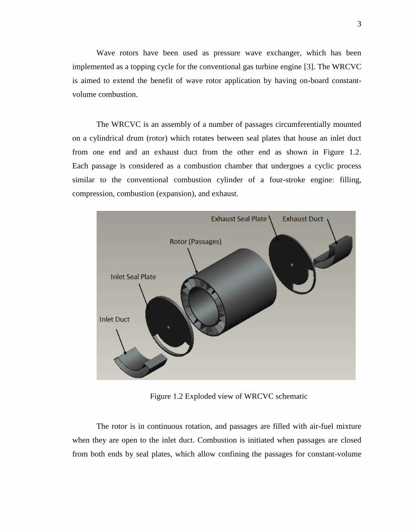
The WRCVC is an assembly of a number of passages circumferentially mounted

on a cylindrical drum (rotor) which rotates between seal plates that house an inlet duct

from one end and an exhaust duct from the other end as shown in Figure 1.2.

Each passage is considered as a combustion chamber that undergoes a cyclic process

similar to the conventional combustion cylinder of a four-stroke engine: filling,

compression, combustion (expansion), and exhaust.

Figure 1.2 Exploded view of WRCVC schematic

The rotor is in continuous rotation, and passages are filled with air-fuel mixture

when they are open to the inlet duct. Combustion is initiated when passages are closed

from both ends by seal plates, which allow confining the passages for constant-volume

4

combustion. Then the combustion product gas is exhausted through the exhaust ports

when the passages are open to the exhaust duct.

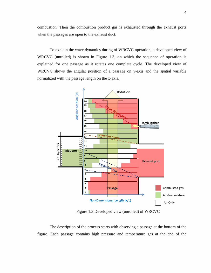
To explain the wave dynamics during of WRCVC operation, a developed view of

WRCVC (unrolled) is shown in Figure 1.3, on which the sequence of operation is

explained for one passage as it rotates one complete cycle. The developed view of

WRCVC shows the angular position of a passage on y-axis and the spatial variable

normalized with the passage length on the x-axis.

Figure 1.3 Developed view (unrolled) of WRCVC

The description of the process starts with observing a passage at the bottom of the

figure. Each passage contains high pressure and temperature gas at the end of the

5

combustion process. The passage starts to open to the exhaust duct as the rotor rotates.

The combusted gas starts to flow out through the exhaust duct and an expansion fan

propagates reducing the pressure inside the passage due to exhaust gas sweep. The

passage is then filled with a stratified air-fuel mixture when it is opened to the inlet duct.

The stratification of the inlet charge is controlled with the fuel filling process. During the

filling process the passage is still open to the exhaust duct for a certain overlap period

which allows purging of exhaust gas.

When the passage closes with the exhaust duct, a hammer shock wave is

generated and propagates from the exhaust side towards the inlet side applying

compression work on the air-fuel mixture in the passage. The design of ports is timed

with the rotational speed so the hammer shock, optimally, arrives to the inlet side when

the passage is closing with the inlet duct. When the passage is closed from both ends, a

hot gas jet is introduced into the passage from the exhaust wall side through a torch jet

injector (torch igniter). Hot gas mixes with the air-fuel mixture and ignition is initiated.

Flame propagates in the constant volume passage, and combustion is to be completed

before the passage starts to open to the exhaust port and start a new cycle. The sequence

is the same for all the passages with a time shift determined by the angular difference

between one passage and another.

The flow is unsteady on a local reference frame of the passage; however,

continuous rotation of the passages allow the synchronization that provides a steady flow

through inlet and exhaust ducts, which is more likely convenient to the operation of gas

turbine engine.

A comprehensive literature review for the wave rotors and their applications are

presented by Akbari et. al [4]. Preliminary studies on the improvements that WRCVC can

offer to improve the performance of gas turbine engines showed that installation of

WRCVC in Rolls-Royce engine AE3007 and operating with pressure gain of 1.55 would

result in a 15% reduction in specific fuel consumption [5]. WRCVC operation with the

6

T56 engine, in its industrial version 501K with pressure gain 1.28 would result in 12%

reduction in specific fuel consumption and 20% increase in the output power [6].

1.2. Previous Work

In the 1990’s Daniel Paxson of NASA developed an unsteady, one-dimensional

numerical model to solve the unsteady gas dynamics of a pressure wave exchanger [7].

Paxson took the initiative to start a simple numerical model that solves inviscid

compressible Euler equations of a calorically perfect gas, which he later developed to

account for losses associated with flow in a wave rotor operation such as frictional losses,

heat transfer, leakage, and other losses [8]. The numerical model was calibrated and

validated with two phases of pressure wave exchanger rigs [9, 10]. Experimental data

from the test rigs have been used to develop semi-empirical formulas for losses modules

in the numerical model [11].

Thereafter Nalim participated with Paxson to develop the numerical model to

include a single step combustion model to simulate wave rotor operation with reactive

charges and on-rotor combustion [12]. The combustion model is capable of a turbulence-

driven deflagration flame propagation, detonation combustion, and deflagration to

detonation transition modes. This model has been used for the aero-thermal design of the

WRCVC rig.

Torch jet penetration (distributed ignition) and circumferential leakage models

have been recently introduced to the WRCVC simulation model in a progress of

validation of the model with experimental data of WRCVC testing. Simulations of the

one-dimensional model, with single-step combustion, have been validated with

experimental data from WRCVC. The model showed good capability in predicting the

operation of WRCVC [13].

7

Stratified charges in Wave Rotor Combustors have been studied by Nalim [14],

which presented a numerical model for multi-species, single-step eddy dissipation

combustion model based on Magnussen’s work [15]. The impact of using a multi-species

to with the single-step model is needed to apply the flammability limits for the ignition

criteria. However, the assumption of a complete combustion of the fuel-oxidant into

products adds up some restrictions on the accuracy of simulating rich mixtures.

1.3. Problem Statement

WRCVC technology has been studied over the past decade by Nalim and his

students in collaboration with Rolls-Royce to demonstrate the viability of applying the

constant-volume combustion in gas turbine engines. Assessments of the preliminary

design of WRCVC were done by a time-dependent, one-dimensional numerical model [1]

[16]. The model is utilized to solve gas dynamics and combustion equations of the

problem. This model has been first introduced for the wave rotor applications by Nalim

and Paxson [12].

The combustion was modeled as a single step reaction where the reaction progress

is indicated by a single variable representing the concentration of reactants. The model

showed good reliability in predicting the combustion and flame propagation over

considerable range of operating conditions. Nevertheless the assumption of complete

conversion of reactants into final combustion products, results in an over-predicted heat

release [17]. The model also assumed a perfectly mixed combustible charge which is not

realistic in the application of WRCVC where the air-fuel mixture is highly stratified in it.

A more detailed (multi-step) combustion model is proposed to substitute the

single-step reaction model to include progress variables for multiple species that involve

the chemical kinetics of the combustion model. The new model would extend the

previous stratified-charge single-step reaction model reported by Nalim [14], which

8

allows taking account for the air-fuel mixtures flammability limits that affects the

extinction of flame propagation.

1.4. Objectives

The main goal of this work is to extend the capabilities of the previous models

used to model the operation of WRCVC by applying a multi-step reaction model, for

stratified charges represented with a multi-species involved in the reaction model. Some

updates of the recent features (e.g. circumferential leakage and distributed ignition) that

have been applied and validated with the single-step model [13].

The impact of using a multi-step reaction model over the current single-step is the

imposed capability of modeling the combustion of rich mixtures in WRCVC accurately.

In fact, the assumption of complete conversion of air-fuel mixture into combustion

products on which the single-step reaction models becomes invalid in case of rich

mixtures.

9

2. NUMERICAL MODEL

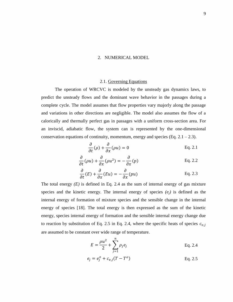
2.1. Governing Equations

The operation of WRCVC is modeled by the unsteady gas dynamics laws, to

predict the unsteady flows and the dominant wave behavior in the passages during a

complete cycle. The model assumes that flow properties vary majorly along the passage

and variations in other directions are negligible. The model also assumes the flow of a

calorically and thermally perfect gas in passages with a uniform cross-section area. For

an inviscid, adiabatic flow, the system can is represented by the one-dimensional

conservation equations of continuity, momentum, energy and species (Eq. 2.1 – 2.3).

( )

( ) Eq. 2.1

( )

( )

( ) Eq. 2.2

( )

( )

( ) Eq. 2.3

The total energy (E) is defined in Eq. 2.4 as the sum of internal energy of gas mixture

species and the kinetic energy. The internal energy of species (ej) is defined as the

internal energy of formation of mixture species and the sensible change in the internal

energy of species [18]. The total energy is then expressed as the sum of the kinetic

energy, species internal energy of formation and the sensible internal energy change due

to reaction by substitution of Eq. 2.5 in Eq. 2.4, where the specific heats of species

are assumed to be constant over wide range of temperature.

∑

Eq. 2.4

( ) Eq. 2.5

10

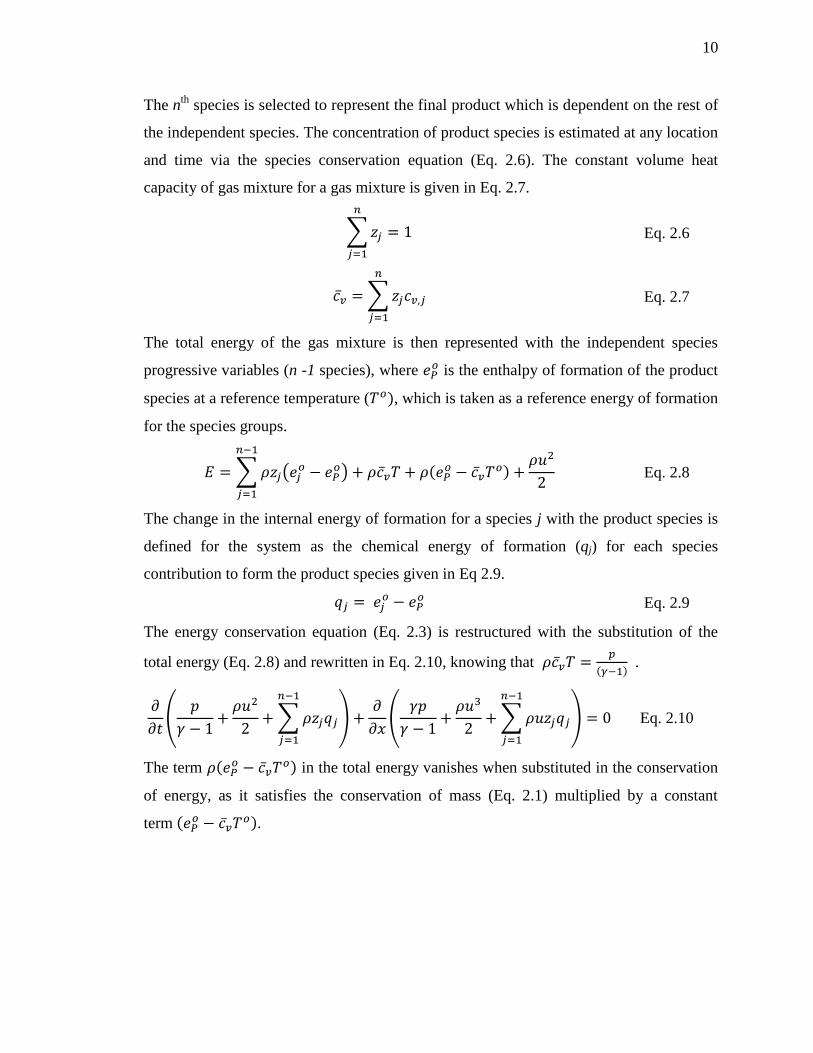
The nth

species is selected to represent the final product which is dependent on the rest of

the independent species. The concentration of product species is estimated at any location

and time via the species conservation equation (Eq. 2.6). The constant volume heat

capacity of gas mixture for a gas mixture is given in Eq. 2.7.

∑

Eq. 2.6

∑

Eq. 2.7

The total energy of the gas mixture is then represented with the independent species

progressive variables (n -1 species), where is the enthalpy of formation of the product

species at a reference temperature ( ), which is taken as a reference energy of formation

for the species groups.

∑ (

)

(

)

Eq. 2.8

The change in the internal energy of formation for a species j with the product species is

defined for the system as the chemical energy of formation (qj) for each species

contribution to form the product species given in Eq 2.9.

Eq. 2.9

The energy conservation equation (Eq. 2.3) is restructured with the substitution of the

total energy (Eq. 2.8) and rewritten in Eq. 2.10, knowing that

( ) .

(

∑

)

(

∑

) Eq. 2.10

The term (

) in the total energy vanishes when substituted in the conservation

of energy, as it satisfies the conservation of mass (Eq. 2.1) multiplied by a constant

term (

).

11

Transport equation for the species associated with the system given as follows:

( )

( )

Eq. 2.11

The presented conservation equations are considered for an inviscid, adiabatic

reactive flow. Viscous, heat transfer, leakage, and turbulence effects are included to the

equations as source terms. The models are presented briefly in this chapter as correction

source terms applied to the system of the governing equations with emphasis on the new

work; however the detailed discussions and the derivations for these source terms are

presented in the Appendix.

2.2. Viscous Effects (Friction)

In real flows, the flow momentum is resisted by a friction force from the passage

walls which is related to the bulk flow properties. The major effect of viscous forces is

near the passage walls where the boundary layer is formed. The boundary layer cannot be

analyzed with one-dimensional equations; hence, the friction is restricted to the shear

stress at the wall. The conservation of momentum equation is then updated with a friction

source term (Eq. 2.12).

( )

( )

( )| ( )|

Eq. 2.12

The friction source term coefficient is defined via a semi-empirical correlation based

on previous work by Paxson [9]. The coefficient is proportional to the passage

geometry and inversely dependent on the Reynolds number of the flow. The complete

derivation of the source term for the friction losses is presented in the Appendix A.

2.3. Heat Transfer

Heat transfer is assumed to be between the working fluid inside the passages and

its upper and lower walls. The heat transfer path is shown in Figure 2.2. The source term

for heat transfer in the energy equation is derived from the Reynolds-Colburn skin-

12

friction analogy. The conservation of energy equation is updated with the source term,

given in Eq. 2.13. The heat transfer source term coefficient is deduced in terms of the

friction source term coefficient as: (

) (

) .

(

( )

∑

)

(

( )

∑

)

( )| ( )|

Eq. 2.13

The derivation of Eq. 2.13 is supplied in the Appendix B.

Figure 2.1 A schematic diagram for heat transfer path in a passage

13

2.4. Turbulence Eddy-Diffusivity Model

The turbulence effects of the flow inside the passage are accounted for in the

governing system with a simplified eddy-diffusivity model. Diffusive fluxes of

momentum, energy and species are calculated based on the gradient of the conserved

parameters. The importance of the turbulence model is its significant role in driving the

diffusive flame propagation.

A simplified turbulence model has been introduced into the one-dimensional

model of wave rotor by Nalim and Paxson [12]. The model allows turbulent diffusion of

mass, momentum, and energy through the turbulent Prandtl number and the turbulent

Schmidt number. The turbulence eddy-diffusivity source terms are applied to the

momentum, energy and species conservation equations as follows:

( )

( )

| |

Eq. 2.14

(

( )

∑

)

(

( )

∑

)

( )| ( )|

(( )

)

(∑

)

Eq. 2.15

( )

( )

Eq. 2.16

The derivation of source terms for the eddy-diffusivity model is in Appendix C.

2.5. Developed Combustion Model

The main objective of this work is to apply a multi-step reaction model for the

combustion process to provide a better representation for the combustion process in wave

rotors. The previous single-step, single-reaction progress variable model is based on an

14

assumption of a perfectly mixed reactant undergoes a complete combustion process. In

the actual operation of WRCVC the combustible mixture is highly stratified with regions

of rich air-fuel mixture and other regions of lean mixture or unfueled air. Hence the flame

propagation is influenced with the flammability limits of the mixture. Other features to

the multi-progress variables reaction model are the flame extinction and incomplete

burning processes that the single-progress variable model cannot model [14].

Various combustion models have been developed to define the paths of fuel break

down and oxidation processes [19]. As the kinetics of the reaction gets more

sophisticated, more species are involved and consequently the computation becomes

expensive with comparatively less benefit. A two-step reaction model with four species is

considered to be an efficient model to be implemented, regarding the level of details

desired and the robustness of the computation [17].

The first step of the reaction mechanism models the partial oxidation process of

fuel into an intermediate species group (Eq. 2.17); thereafter in the second step the

intermediate mixture is oxidized to complete the combustion process (Eq. 2.18). This

model involves four conserved species variables: Fuel, Oxidant, Intermediate and

Product. Species are defined with a scalar variable denoting the mass fraction in the gas

mixture.

The two-step reaction is represented in a generic form for any hydrocarbon fuel

with x molecules of carbon and y molecules of hydrogen oxidized with air.

( ) →

Eq. 2.17

(

) ( )

→

( )

Eq. 2.18

Where the stoichiometric molar quantities for the oxidant a, b are:

15

Eq. 2.19

The species groups (variables) involved in these reactions are defined as follows:

Fuel:

Oxidant:

Intermediate:

Product:

( )

The two-step reaction model can be written in compact notation as:

Step1: →

Step2: →

The species groups are defines as follows:

( )

The species groups are a mixture of compound or radical species. There is a fixed

relationship between the molecular species mass fraction and mass fraction of the species

groups (fuel, oxidant, intermediate, and product). For convenience species groups will be

labeled directly as species in the next discussions.

(

)

(

)

(

)

(

( )

)

(

)

16

(

)

(

)

( ( )

( )

)

The molecular weights of the molecular species are given in Table 2.1.

Table 2.1 Molecular Weight of Species

Species O2 N2 CO CO2 H2O

Molecular

Weight

(kg/kmol)

31.999 28.013 28.010 44.011 18.016

The combustion is modeled to occur in a computational cell only if reactants and

a source of ignition are available. The combustion process is initiated with a temperature-

based ignition model, such that the reaction takes places if the temperature of a cell

exceeds a defined threshold value equivalent to the ignition temperature. The combustion

model is determined to be confined to the least available of reactant species locally in the

numerical cell. The rate of reaction is proportional to the consumption of the least

available species locally; meanwhile a weighting factor is given for the product of each

reaction step for its dominant role in providing active radicals that promote the chemical

reaction. This model eliminates the full consumption of fuel if there is no stoichiometric

amount of oxidant required, as in case of rich mixtures.

The reaction rate of the fuel consumption in reaction step 1 is shown in Eq. 2.20,

and the equivalent amount of oxidant consumed is correlated to the amount of fuel

consumed (Eq.2.21). The sum of fuel and oxidant masses consumed represents the mass

of intermediate species formed in reaction step 1 (Eq. 2.22).

{ (

( ))} Eq. 2.20

17

(

)

Eq. 2.21

Eq. 2.22

The rate of consumption of the intermediate species in the step 2 of reaction is given in

Eq. 2.23, and the equivalent amount of oxidant consumed in step 2 is correlated to the

amount of intermediate consumed as shown in Eq. 2.24.

{ (

( ))} Eq. 2.23

(

)

Eq. 2.24

The total rate of consumption of the oxidant species is the sum of Eq. 2.21 and Eq. 2.24,

while the net rate of formation of the intermediate species is the difference of Eq. 2.23

from Eq. 2.22.

This model accounts for the influence of the intermediate and products species in

driving the reaction rate by diffusion. The model prevents cells from random auto-

ignition when the temperature in these cells exceeds the threshold value, while no

intermediate/product species available locally. The lean flammability limit is considered

in this model to be related to the minimum energy content of the reactants. Hence the

potential static temperature of the mixture after combustion (Eq. 2.25) is the determinant

of whether the mixture is combustible or not.

( ) Eq. 2.25

This approach has been followed by Nalim in a previous study for a numerical model for

stratified combustion in wave rotors [14].

The chemical energy of species (qj) is defined in Eq. 2.9, as the difference

between the internal energy of formation of species and the internal energy of the

products. The internal energy of formation for species is calculated at an average of the

unburned gas temperature and the adiabatic constant volume temperature. The adiabatic

flame temperature is calculated via UVFLAME [20], for ethylene-air rich mixture of

local equivalence ratio 1.273. The calculated adiabatic flame temperature is 2617 K, and

18

the unburned gas temperature is assumed to be 300 K, and the average temperature is

1450 K. The internal energy of formation at 1450 K for the fuel (ethylene), oxidant (air),

intermediate and product is given in Table 2.2.

Table 2.2 Species internal energy of formation at 1450 K

Species Ethylene Air Intermediate Product

(kJ/kg) 1434 - 418 -2870 -3353

In the computational domain, the account for turbulence effects is limited to the

grid size. The turbulence is modeled with a simple eddy-diffusivity model presented in

the previous section. Meanwhile the resolution of a thin moving flame front is not easily

achieved with a uniform grid. The turbulent flame thickness is estimated via a simple

procedure similar to that used to estimate the laminar flame thickness. The turbulent

Prandtl number is assumed to be a unity. The eddy-diffusivity is to be determined based

on the observed combustion rates that are assumed to be controlled primarily by

turbulence intensity. In the present experiments, there is no measurement of the

turbulence levels, and thus no other evidence for turbulence intensity other than the

apparent flame speed or combustion rate. However, by using simple scaling laws, it is

shown that the turbulent flame thickness is independent of the turbulence intensity and

eddy-diffusivity. This allows us to estimate the required grid density without the

knowledge of the turbulence intensity. The turbulent flame thickness is estimated with

the correlation given in Eq. 2.26.

[

( ) ]

Eq. 2.26

The mass consumption of fuel is calculated for the single-step reaction rate based on the

eddy-dissipation reaction model [21]:

{ (

( ))} Eq. 2.27

The unburned gas density is

and the turbulent thermal diffusivity is

. The flame thickness is estimated to be 0.00635 m, thus for accepted

19

resolution for the flame front, 5 - 10 grids should be covered by the flame front.

Therefore, the reasonable grid size is recommended to be at least 0.00125 m for flame

front resolution. The influence of the eddy-diffusivity term on the turbulence parameters

and the reaction rate coefficient is presented in Table 2.3.

Table 2.3 Turbulent Parameters

- (m2/s) (m) (m) (s) (m) (m/s) (1/s)

800 0.05 0.064 0.0064 8.26E-4 0.0064 7.69 4841

1000 0.06 0.064 0.0064 6.61E-4 0.0064 9.61 6051

1500 0.09 0.064 0.0064 4.41E-4 0.0064 14.41 9077

2000 0.12 0.064 0.0064 3.31E-4 0.0064 19.21 12102

3000 0.18 0.064 0.0064 2.21E-4 0.0064 28.82 18154

Other approach for estimating the turbulent flame thickness can be done from the

correlation of the turbulent viscosity given by Hjertager [21]

, where Cμ is a

constant equal to 0.09, k is the kinetic energy of turbulence, and ϵ is the dissipation rate

of kinetic energy of turbulence. Maintaining the assumption of unity Prandtl number, the

turbulent viscosity coefficient can be substituted in terms of turbulent thermal diffusion;

hence the ratio between the dissipation rate of turbulent kinetic energy and the kinetic

energy of dissipation (turbulence timescale) is considered to be

.

The kinetic energy of turbulence is by definition for 1D flow

, where the

root-mean-square of the velocity fluctuations is defined as the turbulence length scale

divided by the turbulence time scale,

. The turbulence length scale is

[22]. The turbulence time scale is presented in terms of passage hydraulic diameter as,

. The turbulent flame thickness can be defined as, √ , thus the

turbulent flame thickness is estimated to be 2% of the hydraulic diameter of the passage

.

20

2.6. Leakage Model

Leakage occurs through the clearance gap between the rotor and stator in

WRCVC, radially from a passage to a casing cavity or the outside atmosphere, and

circumferentially from a passage to another. The friction and heat transfer models are

applied to every discretized cell along the passage; in contrast, the leakage model is

applied only to the terminal cells of the passage as they are assumed to be the source of

gas leaking out and/or the sink for the gas leaking into the passage.

The radial leakage flow is shown in Figure 2.2 with yellow arrows (light) between

the passage and ambient air as two routes with a unified source/sink. The two radial

leakage paths are lumped and modeled as one leakage path assuming the inner and the

outer cavities are connected, and the leakage path lengths are the same. On the other hand

the circumferential leakage occurs between the passage and its neighboring passages

(leading and trailing) is represented by two red arrows (dark) in Figure 2.2. The two

routes of the circumferential leakage are treated seperately since the source and the sink

of both routes are different. The pressure differences driving the circumferential leakage

are small compared to the radial leakage [23]. Nevertheless, the instances where strong

pressure waves propagating inside the passage arrive to the ends of the passages create a

relatively large pressure difference which may drive the circumferential leakage.

Leakage is modeled as a steady flow through an orifice area perpendicular to the

flow stream as shown in Figure 2.5 (a, b). Saint Venant’s orifice equation (Eq. 2.29) is

used to model the leakage mass flow rate [24].

√

*(

)

(

)

+ Eq. 2.28

21

Figure 2.2 Leakage paths from a representing passage of WRCVC

Figure 2.3 A schematic representation for leakage flow through the gap

22

The leakage is represented as a mass source term in the continuity equation over the

control volume of the cell which leakage is occurring (Figure 2.3c).

[ ( ) ( )] Eq. 2.29

The cross-section area for the leakage paths are:

Radial Leakage: ( )

Circumferential leakage: ( )

The average passage width is determined at the passage equal area split.

The leakage mass flow rate for an outflow leakage is applied as follows:

Radial Leakage:

The lumped radial leakage flow is:

√

*(

)

(

)

+ Eq. 2.30

Circumferential leakage:

The outflow leakage from the passage to the leading passage is given:

√

*(

)

(

)

+ Eq. 2.31

The out flow leakage to the trailing passage is given in (Eq. 2.51):

√

*(

)

(

)

+ Eq. 2.32

The total leakage flow flux is the combination of Eq. 2.31, Eq. 2.32, and Eq. 2.33.

These correlations are based on the assumption that the passage is leaking out gas;

however, if the passage is a flow sink and mass leaks into the passage, then the

correlations should be appropriately reverted such that the parameters for the leakage

source becomes sink and vice versa. For such a case the radial leak flow is presented as

shown in Eq. 2.34, and similarly applied to Eq. 2.32 and 2.33 for the similar situation.

23

√

( ) *(

)

(

)

+ Eq. 2.33

The pressure ratio driving the leakage flow is limited by the maximum pressure

ratio that developed a choked flow which is given in (Eq. 2.35) such that higher pressure

differences than the limiting value would result in leakage flow no higher than the choked

flow rate.

(

)

(

)

Eq. 2.34

Energy leakage over the control volume is:

( ) Eq. 2.35

Where the total enthalpy is:

Eq. 2.36

The coefficient of discharge introduced in (Eq. 2.31 – 2.33) is corrected for

turning and velocity losses, where the correction factor (CL) is found as follows (25):

(

)

Eq. 2.37

The entrance velocity loss coefficient (CL) is related to the head loss as follows:

Eq. 2.38

2.7. Non-dimensionalization

The governing equations presented through this chapter became more

sophisticated and much more complicated; thus it is efficient to normalize the primary

variables into a dimensionless form. This process leads to a zero dimension equations that

its solution is adaptable for any units system. The parameters are normalized with

reference values as shown below.

24

Eq. 2.39

The reference pressure is presented by the perfect gas law in terms of reference density,

universal gas constant and reference temperature, which is also presented in another form

in terms of reference speed of sound and specific heat ratio instead of the reference

temperature and the universal gas constant.

Eq. 2.40

The reference time can be presented by the reference length over the reference speed

(speed of sound at reference temperature).

Eq. 2.41

The conservation equations of mass, momentum, energy and species are

normalized with a combination of reference values as follows:

Continuity:

Momentum:

Energy:

Species:

The chemical energy of the species (qj), is normalized with the square of the

reference speed of sound ( ). Some non-dimensional quantities appear when the

governing system of equations is normalized with the reference values. Those quantities

are:

Reynolds Number:

25

Prandtl Number:

Schmidt Number:

2.8. Summary

The governing equations and derivations have been elaborated comprehensively

in this chapter. For convenience the governing system, in this section, is described in a

short hand notation such that vector w represents the conserved parameters while vector f

represents the flux and S is representing source terms. In this section the equations are

given in the dimensionless form without asterisk superscript for convenience.

( )

( ) Eq. 2.42

The conservation and the flux arrays are:

[

( )

∑

]

Eq. 2.43

[

(

( )

∑

)

]

Eq. 2.44

The source term is divided into two vectors; first vector includes source terms

applied to all locations in the passage such as: friction, heat transfer, turbulence and

species conversion (combustion); while the second vector which is typically the leakage

terms (radial and circumferential) is applied to only the passage boundaries.

26

( )

[

| |

(

( ) ∑

) | | ( )

{

} ⟨

⟩]

Eq. 2.45

[

√

*(

)

(

)

+

√

*(

)

(

)

+

√

*(

)

(

)

+]

Eq. 2.46

[

√

( )

√

( )

√

( )

]

Eq. 2.47

(

)

(

)

Where j in (Eq. 2.63) is an index for the leakage sink (lead and trail).

27

3. NUMERICAL SCHEME

The governing system is a hyperbolic partial differential equation (Eq. 2.43), for

which a direct solution is not easily achieved. The differential equation of the governing

system is numerically integrated, to solve for the approximate Riemann problem, with the

explicit, second-order, total variation diminishing (TVD) Lax-Wendroff scheme which is

a second order accurate in time and space. The monotonicity of the solution requires the

scheme to be TVD, which utilizes non-linear functions known as limiters to control the

anti-diffusive flux differences. Roe’s method of flux estimation [26] is applied with the

second order scheme to solve the system. The details of Roe’s method applied in the

model are given in Appendix F.

3.1. TVD Lax-Wendroff Scheme

The Lax-Wendroff one-step second-order scheme is used for integrating the

hyperbolic system of conservation laws. The scheme has reduced its accuracy at points

with extreme fluxes. Some oscillations near discontinuities (jumps) would appear and

would require numerical dissipation [27]. The basic schemes must to be altered by

limiting the flux differences in order to yield a monotonic and sharp representation for

jumps. The anti-diffusive terms considered by a TVD scheme play an important role in

increasing the accuracy and diminishing the total variation. A detailed derivation for the

numerical model and discretization is reported comprehensively in the Appendix E.

The total variation of a mesh solution w is defined as:

( ) ∑|

|

Eq. 3.1

28

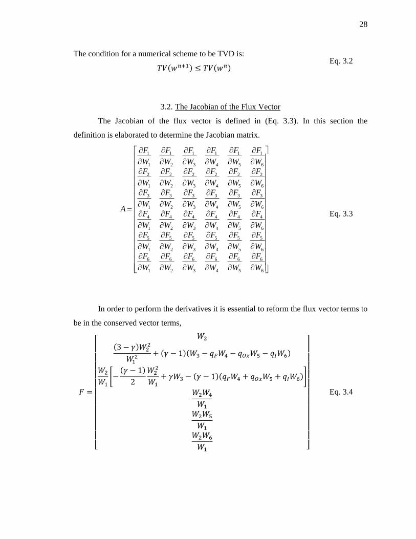
The condition for a numerical scheme to be TVD is:

( ) ( ) Eq. 3.2

3.2. The Jacobian of the Flux Vector

The Jacobian of the flux vector is defined in (Eq. 3.3). In this section the

definition is elaborated to determine the Jacobian matrix.

6

6

5

6

4

6

3

6

2

6

1

6

6

5

5

5

4

5

3

5

2

5

1

5

6

4

5

4

4

4

3

4

2

4

1

4

6

3

5

3

4

3

3

3

2

3

1

3

6

2

5

2

4

2

3

2

2

2

1

2

6

1

5

1

4

1

3

1

2

1

1

1

W

F

W

F

W

F

W

F

W

F

W

F

W

F

W

F

W

F

W

F

W

F

W

F

W

F

W

F

W

F

W

F

W

F

W

F

W

F

W

F

W

F

W

F

W

F

W

F

W

F

W

F

W

F

W

F

W

F

W

F

W

F

W

F

W

F

W

F

W

F

W

F

A Eq. 3.3

In order to perform the derivatives it is essential to reform the flux vector terms to

be in the conserved vector terms,

[

( )

( )( )

*

( )

( )( )+

]

Eq. 3.4

29

Hence, after completing the derivative, the Jacobian matrix is:

Eq. 3.5

3.3. Eigenvalues and Eigenvectors

For a hyperbolic system all the terms of the Jacobian matrix [A] must be real, and

hence it can be diagonalized, where the matrix [R] is the right eigenvectors, and matrix

[L] is the left eigenvectors and the diagonal matrix [Λ] is the eigenvalues which are the

characteristic speeds at which acoustic signals travel in the x – t space. An important

feature to be noted is that the right eigenvectors matrix is the inverse of the left

eigenvectors.

[ ] [ ][ ][ ] Eq. 3.6

The eigenvalues and the right eigenvectors are shown below. The right

eigenvectors matrix is noted as [E] for the convenience of matching Roe’s nomenclature.

au

u

u

u

u

au

~~

~

~

~

~

~~

Eq. 3.7

ii

oxox

ff

iioxoxffioxfiioxoxff

zz

zz

zz

auHzqzqzqqqqu

auHzqzqzq

auuau

E

~1000~

~0100~

~0010~

~~~~~~

2

~~~~~~~

~~000~~~100011

2

Eq. 3.8

30

4. WAVE-ROTOR CONSTANT-VOLUME COMBUSTOR

Based on known documentation, the first pressure wave machine with on-board

combustion was built in the early 1990’s by Asea Brown Boveri (ABB) through a Swiss

government funded project [28]. The ABB wave rotor had 36 passages and was operated

at speeds up to 5000 rpm. The work by ABB showed important attainments in some

aspects as for the method of fueling between premixed and non-premixed. Their study

included various ignition methods such as ignition via spark plugs or auto-ignition via hot

gas jet. In the ABB rig spark plugs were used in the start-up for ignition, then after the

steady operation with combustion, hot combusted gas is re-circulated into the fresh

mixture for ignition. Some important challenges have been addressed and tackled

through the ABB research work such as the control of the leakage through the clearance

gap between the rotor and the stator, and the cooling of the passages with compressed air

to prevent the occurrence of premature combustion.

Application of pressure gain combustion in the wave rotor has been investigated

by NASA. The study included various combustion modes of premixed deflagration, and

non-premixed auto-ignition and detonation [2]. The study is taken further with a

developed time-dependent, one-dimensional numerical model that simulates the

operation of the wave rotor as a combustor. The combustion model was facilitated for

deflagration, detonation, and deflagration-to-detonation transition modes [12].

Rolls-Royce North American Technologies collaborated with IUPUI, to design

and build a new rig to demonstrate the viability of achieving a consistent combustion for

the aviation applications [29]. The new rig is the first experimental study conducted in

the US for the application of wave rotors as constant volume combustors.

31

4.1. Rig Description

The aero-thermodynamic design of the new WRCVC rig was done using a time-

dependent, one-dimensional single species, one-step combustion model using a single

species variable for both deflagration and detonation combustion modes [16]. The new

test rig was completed and tested in 2009 and successful combustion was achieved. The

on-board measurements for the experiment test cases are used in the next chapter to

compare with the simulations for validation.

The WRCVC rig is set up in the facilities of Zucrow labs at Purdue University

and is shown in Figure 4.1. The rotor consists of 20 passages each 31 inches in length,

arrayed circumferentially on a cylindrical drum of inner radius 6.48 inches and the outer

radius of the rotor is 9.09 inches. The details of rotor design and dimensions are given in

Table 4.1. In the numerical model, presented in this work, all the lengths are normalized

to the passage length (30.95 inches). The angular position is prescribed in radians.

Table 4.1 Details of WRCVC rig dimensions

Dimension Value Unit

Number of passages 20 -

Passage Length 31.0 inch

Hub radius 6.48 inch

Tip radius 9.09 inch

Passage height 2.61 inch

Passage hydraulic diameter 2.49 inch

Passage web thickness 0.10 inch

Clearance gap 0.03 inch

Area blockage 4% -

The air-fuel mixture is supplied into the WRCVC through an inlet duct of a

partial-annulus cross-section that starts filling from angular position 0° to 104°.

32

Fuel injectors (15 tubes) are installed in the inlet duct to supply fuel into the air

charged into the rig passages. The fuel flow in these tubes is controlled to obtain the

stratification targeted for testing. A set of guiding vanes are installed at the end of the

inlet duct to turn the flow at the entry of the passages by 18°. The flow turn accounts for

the tangential velocity component of the rotor, thus the inlet flow is ideally axial relative

to the passage frame of reference. The account for flow turning is applied to minimize the

incidence losses, which contribute to pressure loss and flow separation at the inlet side of

the passages. The exhaust port is a semi-annulus duct which is installed to purge

combusted gas from the angular position 316° (-44° from inlet duct) to 75°.

Figure 4.1 WRCVC test rig [30]

The WRCVC uses a torch igniter to ignite the air-fuel mixture inside the passage.

The torch igniter is a nozzle with a small pre-chamber in which a specified portion of air

and fuel (propane) is burned in the pre-chamber, and then the hot combusted gas in the

pre-chamber is supplied into the passages through a convergent divergent nozzle. The

torch igniter is installed at angular position 180° for the tests presented in this work.

33

4.2. WRCVC Operation procedure

The testing procedure for the WRCVC is described as follows:

An electric motor spins the rotor to the targeted speed (2100 rpm) and maintains

the speed constant throughout the entire testing.

After the reaching the targeted speed the main air is turned on, and the flow rate

ramps up to the targeted flow rate, and maintained constant throughout the entire

testing.

When the air flow rate reaches the targeted value the torch igniter is triggered and

hot gas jet is supplied into the rig.

When both air and torch flow rates are constant at the targeted values, the fuel

(ethylene) is injected through the designated fuel tubes (1 – 9 for most of the

tests) which mix locally with the air in the inlet duct.

The combustion occurs during the fueling period (~1.2 sec for most of the tests).

After the fuel is turned off the torch igniter is maintained operating till the end of

the testing.

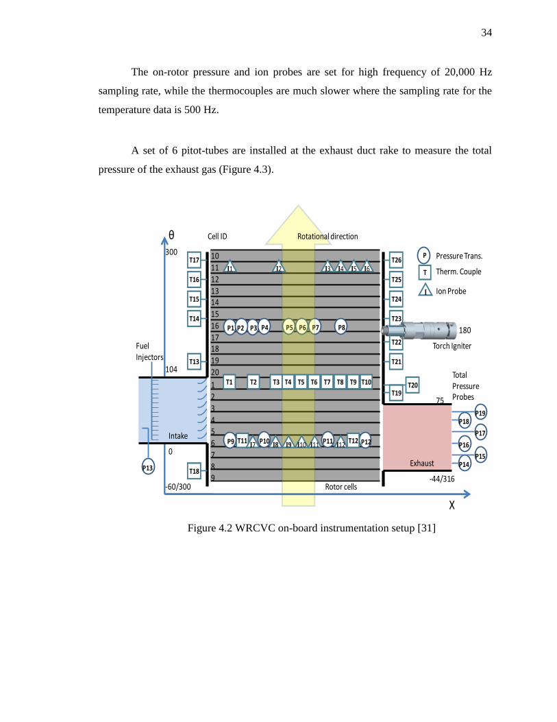
4.3. WRCVC Instrumentations

The rotor is instrumented with high-frequency pressure transducers, measuring

absolute pressure in range 0-500 psia, are installed along passages number 6 and 16 as

shown in Figure 4.3. In addition, the high frequency ion probes are installed in passages

number 6 and 11 (as shown in the developed view of WRCVC in Figure 4.2).

The ion probes detect the ions associated with the combustion; hence, their

signals indicate the presence of the flame at the probe. Considering a number of ion

probes installed along the passage, the flame propagation inside the passage is measured.

The temperature of the gas inside the passages is measured with thermocouples installed

along passages 1 and 6. Also, thermocouples are installed at the end walls seal plates

(inlet and exhaust) to measure the temperature of the gas at seal plates at various angular

positions (Figure 4.2).

34

The on-rotor pressure and ion probes are set for high frequency of 20,000 Hz

sampling rate, while the thermocouples are much slower where the sampling rate for the

temperature data is 500 Hz.

A set of 6 pitot-tubes are installed at the exhaust duct rake to measure the total

pressure of the exhaust gas (Figure 4.3).

Figure 4.2 WRCVC on-board instrumentation setup [31]

0

104

-60/300

300

-44/316

75

P9 P10 P11 P12

P1 P3 P4 P5 P6 P7 P8P2

1

2

3

45

6

7

89

10

11

12

1314

15

16

1718

19

20

P14P15

P16

P17

P18

P13

Cell ID

Total Pressure Probes

Rotor cells

Exhaust

Intake

Rotational direction

Torch Igniter

X

θ

Fuel Injectors

P19

180

T16

T15

T14

T13

T18

T17

T19T20

T21

T22

T23

T24

T25

T26

T12T11

T10T9T8T7T4 T5 T6T3T2T1

I1 I2 I3 I5I4 I6

I7 I8 I9 I10 I11 I12

I

T

P Pressure Trans.

Therm. Couple

Ion Probe

35

Figure 4.3 Pitot-tubes setup at exhaust duct rake in WRCVC

4.4. Adapting Friction Factor for WRCVC Rig

The friction model in the unsteady one-dimensional numerical solver presented in

chapter 2 (Eq. 2.12) is adapted empirically according to NASA experiments conducted on

a wave rotor pressure exchanger. The friction coefficient is highly dependent on the rotor

(passage) geometry, and consequently the friction model for WRCVC is expected to be

different from NASA’s rig.

The parameters affecting rotor friction include passage geometric aspect ratio as

for width and height which are defined by the number of passages, rotor tip diameter and

the hub-to-tip ratio. Other factors that affect the friction are the passage length and

hydraulic diameter which are already considered in the friction coefficient [32]. The

friction losses increase as the number of passages increase. The hub-to-tip ratio governs

the aspect ratio of the passage profile, which is partially considered with the hydraulic

diameter. Although blockage losses are not included into the friction losses, blockage

36

reduces the net flow area of the passage which increases the velocity of the flow (for a

constant mass flow), and subsequently the friction losses increase.

Paxson introduced a semi-empirical friction factor (Eq. 4.1) [9] that was validated

on experimental data from previous wave rotor research work of GE [33], and Kentfield

[34]. The friction loss source term is Sfriction= ζ2u|ρu|1-η

, and 1 – η = 0.5. The friction

correlation was updated by Paxson after collecting more experimental data from the

NASA rig phase I (Eq. 4.2 and 4.4), where 1 – η in the friction loss source term is 0.75

[35, 36]. The turbulent skin friction coefficient introduced by Schlicting (1979) [37]

shown in Eq. 4.4 which is, according to Wilson, valid to a wide range of NASA’s rig

configurations [23]. The friction losses is later adjusted by Paxson for Phase II rig (Eq.

4.5) where 1 – η = 0.8.

Paxson 1993: 1 – η = 0.5 (

) Eq. 4.1

Paxson 1995: 1 – η = 0.75 (

)

Eq. 4.2

Paxson 1996: 1 – η = 0.75 (

)

Eq. 4.3

Wilson 1997: 1 – η = 0.75 (

)

Eq. 4.4

Paxson

(unpublished): 1 – η = 0.8 (

)

Eq. 4.5

The friction factor for WRCVC in (Eq. 4.5) is based on NASA’s rig; hence, it is

more suitable to seek a corrected correlation to account for geometry differences.

Comparison between the WRCVC and NASA’s rigs for the parameters affecting the

friction is shown in Table 4.2.

The comparison from the geometrical differences showed that the friction loss in

the WRCVC passages is should be equivalent to 90% of the actual frictional losses in the

37

passages of NASA’s rig. Hence the friction coefficient suggested for WRCVC is given

in Eq. 4.6.

(

)

Eq. 4.6

Table 4.2 Comparison between WRCVC rig and NASA phase I rig

Parameter WRCVC rig NASA rig

(Phase I)

Number of passages per cycle 20/1 130/1

Tip diameter (in) 9.090 12.00

Hub-to-tip ratio 0.713 0.933

Blockage factor 0.0403 0.0690

The proposed correlation agrees with the ratio of Kentfield correlation with

Paxson (1993), regarding that WRCVC passage geometry and number of passages is

close to Kentfield rig [9]. The new correlation is plotted with the correlations found in

literature for length to hydraulic diameter equal to 12.43 in the WRCVC.

Figure 4.4 Friction coefficient semi-empirical correlations (1-η = 0.5)

Reynolds No. (Re)

2

Kentfield(1969)

GE(1960)

Paxson(1993)

38



Reynolds No. (Re)

2

Paxson(1995)

Paxson(1996)

Schlicting(1979)

105

106

107

108

109

10-2

10-1

100

Reynolds No. (Re)

2

Paxson (unpublished)

WRCVC(2011)

39

5. SIMULATIONS AND COMPARISONS

The numerical model described in chapter 2 is tested with the combustion model

prescribed in section 2.5. The combustion model for the time-dependent, one-

dimensional simulations of the WRCVC is provided with the two-step reaction model

with three independent species: Fuel, Oxidant, and Intermediate. Simulations of the one-

dimensional model with various configurations of the applied two-step combustion model

are presented in this chapter to demonstrate the new capabilities and verify the model’s

applicability.

The numerical model is utilized to simulate test cases equivalent to the

experimental runs done on the WRCVC rig. One of the challenges in simulating these

test cases is that there is no direct measure for the inlet pressure at the rotor. Therefore,

the simulations are based on matching the mass flow rates supplied to WRCVC from the

inlet port and the torch igniter, as measure at upstream locations. The exit boundary

conditions are assumed to be atmospheric as the exhaust is purged to the atmosphere

through a short duct. The inlet boundary conditions are selected through an iterative

procedure to match the flow rate of the actual experimental test.

The biggest challenge is the lack of information about the turbulence levels of the

flow inside the WRCVC passages which highly influence the combustion rate. Thus the

eddy diffusivity and the corresponding reaction rate coefficient must be estimated by

matching the experimental data.

40

Another intrinsic challenge in modeling the combustion process is the ignition

model. The air-fuel mixture is ignited by the means of a hot gas jet which is injected in

the passage. The hot jet mixes with air fuel mixture and ignites the mixture. The ignition

location and timing is hardly known a priori for a highly transient device like the

WRCVC. The mixing process between the hot jet and the air-fuel mixture is greatly 3D

[38, 39].

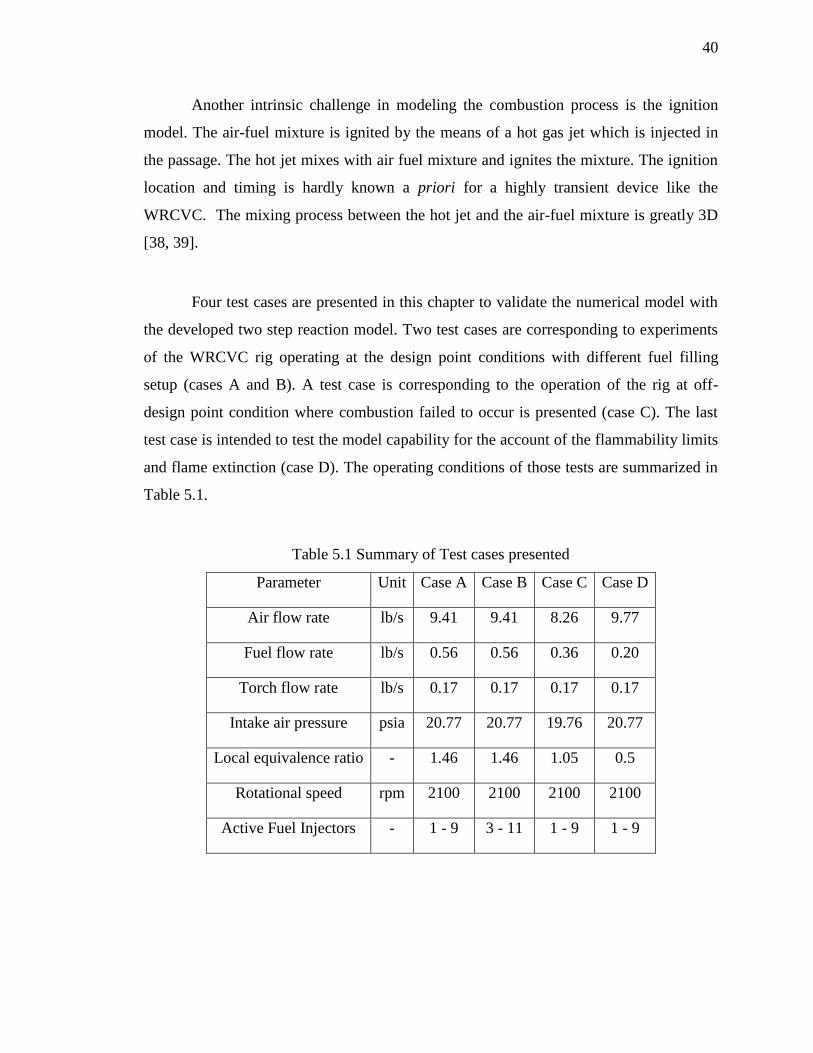
Four test cases are presented in this chapter to validate the numerical model with

the developed two step reaction model. Two test cases are corresponding to experiments

of the WRCVC rig operating at the design point conditions with different fuel filling

setup (cases A and B). A test case is corresponding to the operation of the rig at off-

design point condition where combustion failed to occur is presented (case C). The last

test case is intended to test the model capability for the account of the flammability limits

and flame extinction (case D). The operating conditions of those tests are summarized in

Table 5.1.

Table 5.1 Summary of Test cases presented

Parameter Unit Case A Case B Case C Case D

Air flow rate lb/s 9.41 9.41 8.26 9.77

Fuel flow rate lb/s 0.56 0.56 0.36 0.20

Torch flow rate lb/s 0.17 0.17 0.17 0.17

Intake air pressure psia 20.77 20.77 19.76 20.77

Local equivalence ratio - 1.46 1.46 1.05 0.5

Rotational speed rpm 2100 2100 2100 2100

Active Fuel Injectors - 1 - 9 3 - 11 1 - 9 1 - 9

41

The solution grid independence is studied for a test case (case A) which is

presented later in this chapter. The simulation for that case is tested for different spatial

meshes, while the temporal mesh is changed accordingly to maintain the same Courant

number; thus the numerical stability of the model ensured.

The average pressure of the passage is considered to determine the whether the

solution is grid independent or not. The average pressure of the passage is computed as

the arithmetic mean of the local pressures at each numerical cell, which is calculated at

each time step. The passage average pressure is plotted versus the angular position for

simulations with 100, 200, 400, 600, 800 and 1000 grids in Figure 5.1. The simulation

with 800 grids deemed to present a grid independent solution. The local pressure at the

center point of the passage (x/L = 0.5) is plotted for the simulations of 800 and 1000

grids for verification in Figure 5.2. The local pressure at the passage center verifies that

the simulation with 800 grids presents a grid independent solution.

This is consistent with the estimate of grid density made from the estimate of

turbulent flame thickness, presented in chapter 2. It is also evident that the high level of

grid density is required only for the phase of the cycle when combustion occurs (~180° to

300°), and the lower grid density computations are quite adequate for grid independence

when there is no combustion.

42

Figure 5.1 Average pressure for grid indpendence

Figure 5.2 Pressure trace at passage center point for grid independent solution

0 60 120 180 240 300 3600

10

20

30

40

50

60

70

80

90

100

Angular Position [degrees]

Pre

ssure

[psia

]

100 grids

200 grids

400 grids

600 grids

800 grids

1000 grids

0 60 120 180 240 300 3600

10

20

30

40

50

60

70

80

90

100


Pre

ssure

[psia

]

800 grids

1000 grids

43

5.1. Test Case A

The first test case selected for simulation was operated with targeted rotor speed

2100 rpm. The main air flow rate was supplied at flow rate 9.42 lb/s. Ethylene fuel was

injected at total flow rate 0.56 lb/s, through the first 9 injectors (Figure 5.3). The torch

igniter was set to inject hot gas jet at a flow rate 0.17 lb/s.

(a) Fuel injection stratification (b) Unwrapped inlet duct

Figure 5.3 Stratified fuel filling (case A)

The experimental data from the test case can be examined to have an estimate for

the apparent ignition location, the apparent flame propagation speed and pressure wave

propagation speed in the channels. The data from ion probes are used to locate the flame

front propagation along the passage. The locations of ion probes setup in passage 6 is

shown in Figure 5.4. The ion probes data of a representative cycle for test case A are

shown in Figure 5.5

A signal from ion probe IP12 (nearest to exit wall) was captured at 177°

indicating the presence of flame (reaction zone), then a signal was recorded by IP11 at

186°. A signal from IP10 was recorded at 190° and from IP9 at 192°. Ion probe IP8 gave

multiple signals, which is anticipated to occur due to the sloshing motion of the gas inside

the passage. This sloshing motion is due to the reflection of the pressure wave of

44

combustion from the inlet side wall. An interesting capture from the ion probe data is a

second signal from IP12 at a later time (~206°) with multiple peaks.

Figure 5.4 Ion probes setup in passage 6

Figure 5.5 Measurement of ion probes from passage 6 (case A)

The data from the pressure transducers in passage 16 are used to study the

pressure rise due to combustion and the propagation of the pressure wave for the same

representative cycle. The pressure data from the pressure transducers PT6, PT5, PT3 and

PT2 are used to capture the pressure wave propagation (Figure 5.6). The first evidence of

combustion–generated pressure is examined by comparing the pressure trace of a cycle

before the starting the combustion event, with the pressure traces from the combustion

160 170 180 190 200 210 220 230 2400

0.05

0.1

0.15

0.2

Cycle 8


Ion S

ignal [v

olts]

IP12

IP11

IP10

IP09

IP08

IP07

45

cycle. The pressure rise due to combustion is recorded by PT6 at 182°, PT5 at 184°, PT3

at 190° and PT2 at 192°. These records from ion probes and pressure transducers show

that the combustion is occurring near the exit wall region and propagate towards the inlet

wall side.

Figure 5.6 Pressure transducers setup in passage 16

Figure 5.7 Measurement of pressure transducers from passage 16 (case A)

The ignition location is defined as a point at which the combustion process is

initiated and a flame and a pressure wave are originated at this location, and propagate at

different speeds. The signal timing from ion probes and pressure transducers are plotted

0 30 60 90 120 150 180 210 240 270 300 330 3600

10

20

30

40

50

60

70

80

90

100


Pre

ssure

[psia

]

PT6

PT5

PT3

PT2

46

with the equivalent locations for each measurement probe installed in the passage as

shown in Figure 5.8. Since the characteristics of the flame is highly 3 dimensional, which

affect the ion probes reading, and taking into the account for signal duration, the

uncertainty of the signal timing in Figure 5.8 is represented with a yellow box around the

timing point. The ignition location is projected by extrapolating the trend lines of the

propagation apparent speed for the flame and the pressure wave. The apparent ignition

location is estimated to occur at location x/L = 0.8 and angular position θ = 175°. The

details of this analysis are presented in previous work [30].

Figure 5.8 Apparent ignition location estimate (case A)

The simulation for case A is considered with the estimated ignition location, such

that the distributed ignition model is activated for the numerical cell which is located at

x/L = 0.8. The boundary conditions of the simulation are presented in Table 5.2.

The results of the simulation from the one-dimensional model are presented in the

developed view of WRCVC representing one cycle as shown in Figures 5.3 and 5.4. The

cycle starts at angular position -62° and ends at 288°. The seal plates (walls) are

represented with a black line on both sides. Inlet (0° to 104°) and exhaust (-44° to 75°)

160

165

170

175

180

185

190

195

200

0 0.2 0.4 0.6 0.8 1

An

gula

r P

osi

tio

n (θ

) d

egr

ee

s

Position (x/L)

Pressure Transducers Data

Ion Probes Data

47

ports are represented with white lines on both ends. The torch jet igniter, indicated with

an arrow head, is installed at angular position 180°. However, the igniter has a finite

thickness and a recess socket in the seal plate; hence, the passage starts to open to the

torch igniter at 168°. The results are presented in the dimensionless form, which are

normalized to the same reference values presented in Table 5.2.

Table 5.2 Boundary conditions of simulation of case A

Parameter Dimensionless Dimensional (Unit)

Inlet total pressure 1.22 17.9 (psia)

Inlet total temperature 1.0 520 (R)

Exhaust static pressure 1.0 14.7 (psia)

Exhaust static temperature 1.0 520 (R)

Torch total pressure 8.8 129.3 (psia)

Torch total temperature 6.0 3120 (R)

Other user defined parameters are given in Table 5.3. The coefficient of discharge

of leakage flow was determined by calibration of the simulation of cold flow (no

combustion) data from WRCVC. The coefficient of discharge 0.8 was determined to give

the best match for the experimental data. For simplicity this value is set for both radial

and circumferential leakages.

Table 5.3 User defined parameters

Parameter Value

Coefficient of discharge (CD) 0.8

Turbulent Prandtl Number (Prt) 1.0

Turbulent Schmidt Number (Sct) 1.0

Turbulent eddy-diffusivity (εt) 2500

Reaction rate coefficient step 1 (kr1) 100

Reaction rate coefficient step 2 (kr2) 100

48

The reaction rate coefficient is calculated equivalent to the reaction rate used by

Magnussen and Hjertager [21], which is inversely proportional to the turbulence time

scale. The turbulent viscosity coefficient Cμ (equals to 0.09) in the Kolmogorov-Prandtl

equation did not present a good match with the experimental data. The standard value has

been practically used for the planar jets and mixing layers, and deemed to be not accurate

for other applications as stated by Launder and Spalding [40].

The coefficient is calibrated with a set experimental data from WRCVC. The

simulation results present a reasonable match when the turbulent viscosity coefficient is

magnified 3 – 4 times, where the value 0.35 presents the best match for the currently

available data. The eddy-diffusivity term corresponding to the reaction rate calibrated

with the experimental data (Kr = 100) is equal to 2500, according to the calculations

presented in Chapter 2 (Table 2.3). For consistency, these user defined parameters (Table

5.3) will be maintained the same for the rest of the simulations presented in this chapter.

The results of the simulation in Figure 5.9 present the velocity profile at the inlet

and exhaust ports, contour plot of the temperature (dimensionless) and the log pressure

(dimensionless) inside the passage. The concentration fuel, oxidant and intermediate

species are also presented in contour plots over the developed view in Figure 5.10.

The air-fuel mixture stratification is set to be non-uniform to demonstrate the

capability of the reaction model in dealing with such a problem. The cycle presents a

complete conversion of fuel species (ethylene) into intermediate species (CO + H2O +

N2), via the consumption of a stoichiometric amount of the oxidant (air) required to

complete reaction step 1. Thereafter the intermediate species undergo further oxidation

reaction step 2 to complete the combustion process and the formation of the product

species (CO2 + H2O + N2).

The velocity profile at the exhaust duct show a backflow at angular position ~10°

which is interpreted to be due to the reflection of the expansion fan off the exhaust port as

49

a compression wave, which later (at ~35°) results in backflow at the inlet port. It is noted

from Figure 5.10 that some of the fuel charged into the rig is spilled out through the

exhaust port during the overlap period (the period during which a passage is open to both

inlet and exhaust ports). This spillage is estimated by simulation to be 8% of the total fuel

supplied. Spillage occurs when fuel is supplied from the injectors 1- 9 (i.e. from 0° to

62°)

Figure 5.9 Fluid properties simulation contour plots (case A)

The utilization of the ignition location to occur at x/L = 0.8, a side to the ignition

initiation form the exit wall side from the torch resulted in a rapid rate of reaction for the

air-fuel mixture in the region from x/L = 0.8 to the inlet wall side. On the other hand, a

marginal reaction rate of combustion is seen for the air-fuel mixture closer to the exit

wall side which result in arrival of a second flame to IP12 at later times as seen in the ion

probe IP12 signals (Figure 5.4).

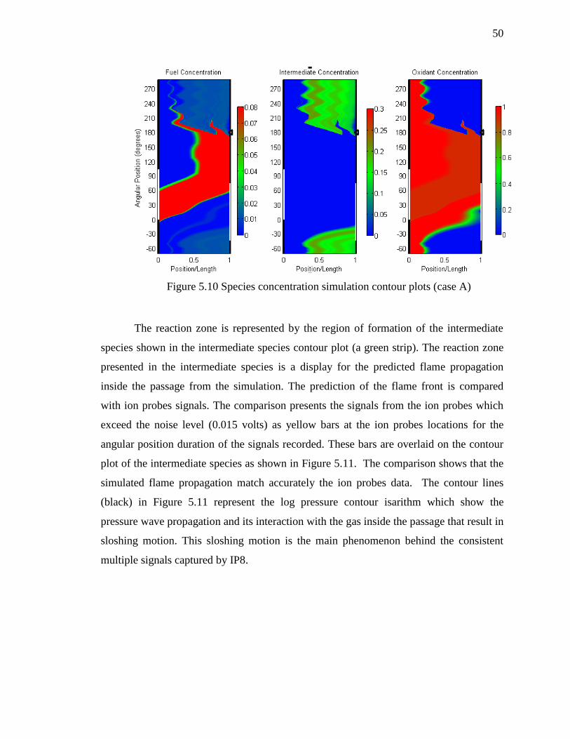
50

Figure 5.10 Species concentration simulation contour plots (case A)

The reaction zone is represented by the region of formation of the intermediate

species shown in the intermediate species contour plot (a green strip). The reaction zone

presented in the intermediate species is a display for the predicted flame propagation

inside the passage from the simulation. The prediction of the flame front is compared

with ion probes signals. The comparison presents the signals from the ion probes which

exceed the noise level (0.015 volts) as yellow bars at the ion probes locations for the

angular position duration of the signals recorded. These bars are overlaid on the contour

plot of the intermediate species as shown in Figure 5.11. The comparison shows that the

simulated flame propagation match accurately the ion probes data. The contour lines

(black) in Figure 5.11 represent the log pressure contour isarithm which show the

pressure wave propagation and its interaction with the gas inside the passage that result in

sloshing motion. This sloshing motion is the main phenomenon behind the consistent

multiple signals captured by IP8.

51

Figure 5.11 Flame propagation comparison (case A)

The comparison between the simulated pressure traces inside the passages and the

experimental data from the pressure transducers are shown for PT2, PT3, PT4, PT5, PT6

and PT8 in Figures 5.10 – 5.15 respectively. The simulated pressure traces are plotted for

the locations x/L equivalent to the positions of the pressure transducers in passage 16

(Figure 5.6). The angular position of the passage for the pressure traces are rescaled to be

from 0° to 360° in order to be adapted to the measured angular position from the

WRCVC encoder.

52

Figure 5.12 Pressure traces comparison at PT2 (case A)


0 60 120 180 240 300 3600

20

40

60

80

100

120Comparison of pressure traces at PT2


Pre

ssure

[psia

]

Experiment

Simulation

0 60 120 180 240 300 3600

20

40

60

80

100



Pre

ssure

[psia

]

Experiment

Simulation

53



0 60 120 180 240 300 3600

20

40

60

80

100



Pre

ssure

[psia

]

Experiment

Simulation

0 60 120 180 240 300 3600

20

40

60

80

100



Pre

ssure

[psia

]

Experiment

Simulation

54



0 60 120 180 240 300 3600

20

40

60

80

100



Pre

ssure

[psia

]

Experiment

Simulation

0 60 120 180 240 300 3600

20

40

60

80

100



Pre

ssure

[psia

]

Experiment

Simulation

55

The comparison between the experimental data and the simulation shows a

reasonable good match, which shows that the simulation gives a fairly well insight for the

process of WRCVC operation. The comparison of the measured temperature and the

simulated temperature is not feasible due to the very slow response of thermocouples in

capturing the variations and changes in the temperature compared to the high frequency

pressure transducers and ion probes. It is noted that the level of noise in the experimental

data from PT8 is much greater than the rest of the transducers. This is due to the thermal

effects on the instrumentations, since PT8 is in the hot zone for most of the testing period.

Pitot-tubes installed at the exhaust duct rake shown in Figure 5.18 were used to

measure the total pressure of the exhaust gas exiting the duct. Pressure measurements

recorded during combustion are shown in Figure 5.19. Since simulation represents an

average cycle for steady operation of WRCVC, those traces are averaged and compared

to the predicted total pressure at the exit (neglecting pressure drop across the duct). The

comparison in Figure 5.20 shows good agreement between averaged experimental data

and simulation traces

Figure 5.18 Pitot-tubes measurements at exhaust duct rake in WRCVC (case A)

214.4 214.5 214.6 214.7 214.8 214.9 215 215.110

15

20

25

30

35

40Exhaust total pressure

Time (s)

Pre

ssure

(psia

)

320 deg

340 deg

0 deg

20 deg

40 deg

60 deg

56

Figure 5.19 Comparison of total pressure at the exit of exhaust duct (case A)

5.2. Test Case B

The second test case targeted for the analysis was run at the same flow conditions

of case A. The only difference is the fuel stratification in the inlet charge. In this test case

the first two fuel injectors were turned off and the fuel was supplied through injectors 3 –

11 (Figure 5.20). This test was targeted to run without fuel spillage during the overlap

period. Since the targeted flow rates for case B was the same for case A, the simulation

for case B is done similar to case A, where the boundary conditions and the arbitrary

user-defined variables are maintained the same.

The simulation shows that no fuel spillage occurred for this test run (Figure 5.22).

By comparing pressure peaks for cases A and B, the effect of 8% fuel spillage resulted in

~25% reduction in pressure rise inside the passage, also simulations showed ~12%

reduction in the overall pressure gain.

-40 -20 0 20 40 6010

15

20

25

30

35

40

45

Angular Position (degrees)

Pre

ssure

(psia

)

Experiment

Simulation

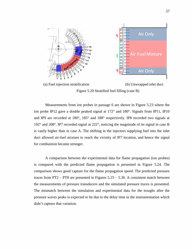
57

(a) Fuel injection stratification (b) Unwrapped inlet duct

Figure 5.20 Stratified fuel filling (case B)

Measurements from ion probes in passage 6 are shown in Figure 5.23 where the

ion probe IP12 gave a double peaked signal at 172° and 180°. Signals from IP11, IP10

and IP9 are recorded at 180°, 185° and 188° respectively. IP8 recorded two signals at

192° and 208°. IP7 recorded signal at 222°, noticing the magnitude of its signal in case B

is vastly higher than in case A. The shifting in the injectors supplying fuel into the inlet

duct allowed air-fuel mixture to reach the vicinity of IP7 location, and hence the signal

for combustion became stronger.

A comparison between the experimental data for flame propagation (ion probes)

is compared with the predicted flame propagation is presented in Figure 5.24. The

comparison shows good capture for the flame propagation speed. The predicted pressure

traces from PT2 – PT8 are presented in Figures 5.25 – 5.30. A consistent match between

the measurements of pressure transducers and the simulated pressure traces is presented.

The mismatch between the simulation and experimental data for the troughs after the

pressure waves peaks is expected to be due to the delay time in the instrumentation which

didn’t capture that variation.

58

Figure 5.21 Fluid properties simulation contour plots (case B)

Figure 5.22 Species concentration simulation contour plots (case B)

59

Figure 5.23 Measurement of ion probes from passage 6 (case B)

Figure 5.24 Flame propagation comparison (case B)

160 170 180 190 200 210 220 230 2400

0.02

0.04

0.06

0.08

0.1

0.12

0.14

0.16

0.18

0.2

Cycle 12


Ion S

ignal [v

olts]

IP12

IP11

IP10

IP09

IP08

IP07

60

Figure 5.25 Pressure traces comparison at PT2 (case B)


0 60 120 180 240 300 3600

20

40

60

80

100

120

140



Pre

ssure

[psia

]

Experiment

Simulation

0 60 120 180 240 300 3600

20

40

60

80

100

120

140



Pre

ssure

[psia

]

Experiment

Simulation

61



0 60 120 180 240 300 3600

20

40

60

80

100

120

140



Pre

ssure

[psia

]

Experiment

Simulation

0 60 120 180 240 300 3600

20

40

60

80

100

120

140



Pre

ssure

[psia

]

Experiment

Simulation

62



0 60 120 180 240 300 3600

20

40

60

80

100

120

140



Pre

ssure

[psia

]

Experiment

Simulation

0 60 120 180 240 300 3600

20

40

60

80

100

120

140



Pre

ssure

[psia

]

Experiment

Simulation

63

The measurements of pitot-tubes at the exit rake of the exhaust duct are presented

in Figure 5.31. The comparison between the simulated total pressure at the exhaust port

and the average of the total pressure measured is presented in Figure 5.32. The

comparison shows a good match between experimental data and the simulation, although

the numerical model assumes uniform conditions at the ports boundaries which is not

always the case in reality.

Figure 5.31 Pitot-tubes measurements at exhaust duct rake in WRCVC (case B)

214.4 214.5 214.6 214.7 214.8 214.9 215 215.1 215.2 215.310

15

20

25

30

35

40

45

50

55Exhaust total pressure

Time (s)

Pre

ssure

(psia

)

320 deg

340 deg

0 deg

20 deg

40 deg

60 deg

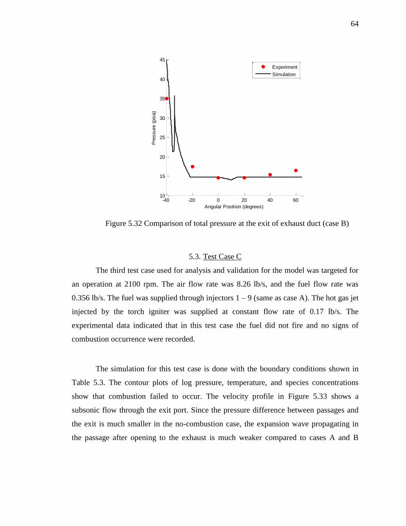
64

Figure 5.32 Comparison of total pressure at the exit of exhaust duct (case B)

5.3. Test Case C

The third test case used for analysis and validation for the model was targeted for

an operation at 2100 rpm. The air flow rate was 8.26 lb/s, and the fuel flow rate was

0.356 lb/s. The fuel was supplied through injectors 1 – 9 (same as case A). The hot gas jet

injected by the torch igniter was supplied at constant flow rate of 0.17 lb/s. The

experimental data indicated that in this test case the fuel did not fire and no signs of

combustion occurrence were recorded.

The simulation for this test case is done with the boundary conditions shown in

Table 5.3. The contour plots of log pressure, temperature, and species concentrations

show that combustion failed to occur. The velocity profile in Figure 5.33 shows a

subsonic flow through the exit port. Since the pressure difference between passages and

the exit is much smaller in the no-combustion case, the expansion wave propagating in

the passage after opening to the exhaust is much weaker compared to cases A and B

-40 -20 0 20 40 6010

15

20

25

30

35

40

45

Angular Position (degrees)

Pre

ssure

(psia

)

Experiment

Simulation

65

where combustion occurred. The reflection of the expansion wave did not cause a

backflow at the exhaust port, however it stagnated the flow at position ~15°.

Table 5.4 Boundary conditions of simulation of case C

Parameter Dimensionless Dimensional (unit)

Inlet total pressure 1.18 17.3 (psia)

Inlet total temperature 1.0 520 (R)

Exhaust static pressure 1.0 14.7 (psia)

Exhaust static temperature 1.0 520 (R)

Torch total pressure 8.8 129.3 (psia)

Torch total temperature 6.0 3120 (R)

The failure of combustion occurrence is reasoned to be due to that the air-fuel mixture

did not reach all the way to the exit wall side, thus the combustible mixture was not

located in the vicinity of the torch jet injection as shown in Figure 5.34.

Figure 5.33 Fluid properties simulation contour plots (case C)

66

Figure 5.34 Species concentration simulation contour plots (case C)

The pressure traces (experimental data) show that no significant pressure rise due

to a combustion event is recorded. The comparison between pressure traces of PT2, PT3,

PT4, PT5, PT6 and PT8 is shown in Figures 5.35 – 5.40. The comparisons show a good

agreement between the experimental data and the predicted traces from simulation. Some

discrepancies appear between the simulated pressure traces and the experiments, during

the filling and purging time processes, which is relied to be due to the assumption of a the

uniformity of the boundary conditions, which is not essentially to the case for the actual

run, where the non-uniformity in the boundary conditions is expected. The simulation

presents an average cycle for the steady operation of WRCVC. However for a highly

transient device like WRCVC, the conditions of a previous cycle might affect the next

one.

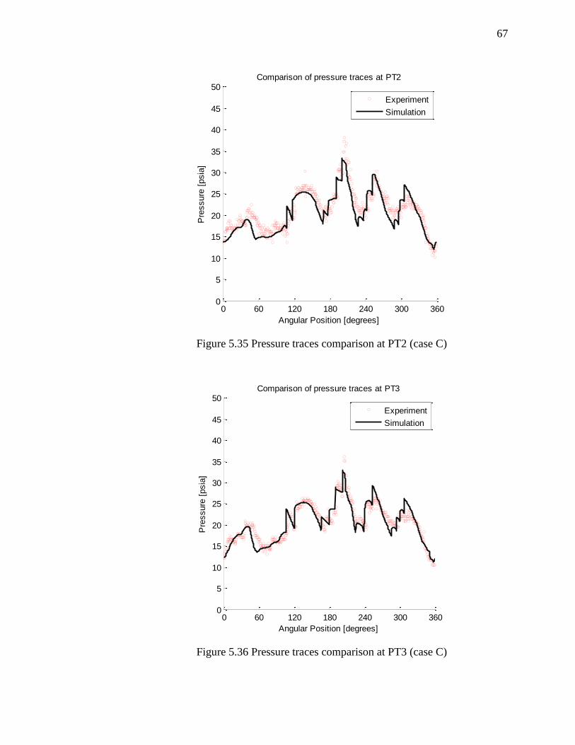
67

Figure 5.35 Pressure traces comparison at PT2 (case C)


0 60 120 180 240 300 3600

5

10

15

20

25

30

35

40

45



Pre

ssure

[psia

]

Experiment

Simulation

0 60 120 180 240 300 3600

5

10

15

20

25

30

35

40

45



Pre

ssure

[psia

]

Experiment

Simulation

68



0 60 120 180 240 300 3600

5

10

15

20

25

30

35

40

45



Pre

ssure

[psia

]

Experiment

Simulation

0 60 120 180 240 300 3600

5

10

15

20

25

30

35

40

45



Pre

ssure

[psia

]

Experiment

Simulation

69



0 60 120 180 240 300 3600

5

10

15

20

25

30

35

40

45



Pre

ssure

[psia

]

Experiment

Simulation

0 60 120 180 240 300 3600

5

10

15

20

25

30

35

40

45



Pre

ssure

[psia

]

Experiment

Simulation

70

5.4. Test Case D

The combustion model in this case is tested for fuel-air charges leaner than the

lean flammability limit of ethylene fuel. In this test, case A is repeated with fuel-air

mixture at equivalence ratio 0.3. For case A at equivalence ratio 0.3 the fuel mass fraction

(zf) is 0.02 and the oxidant mass fraction (zox) is 0.98. This mixture is assumed to be non-

combustible knowing that the lean flammability limit of ethylene is 0.4 [41].

The simulation results, in Figures 5.41 and 5.42, show that combustion was not

developed; even though the air-fuel mixture reached the end wall side and was at the

vicinity of the torch jet. The pressure traces at PT2 and PT5 are presented in Figures 5.43

and 5.44 show that the pressure traces are similar to the pressure traces presented in case

C where combustion also failed to occur.

Figure 5.41 Fluid properties simulation contour plots (case D)

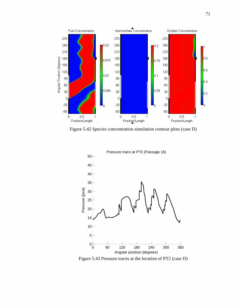
71

Figure 5.42 Species concentration simulation contour plots (case D)

Figure 5.43 Pressure traces at the location of PT2 (case D)

0 60 120 180 240 300 3600

5

10

15

20

25

30

35

40

45

50Pressure trace at PT2 (Passage 16)

Angular position (degrees)

Pre

ssure

(psia

)

72

Figure 5.44 Pressure traces at the location of PT2 (case D)

0 60 120 180 240 300 3600

5

10

15

20

25

30

35

40

45

50Pressure trace at PT5 (Passage 16)

Angular position (degrees)

Pre

ssure

(psia

)

73

6. CONCLUSIONS AND RECOMMENDATIONS

6.1. Conclusions

The time-dependent, one-dimensional numerical model used to simulate the

operation of WRCVC has been developed to include a two-step reaction model. The two-

step reaction model with four species variables offer a satisfactory level of detail

necessary for modeling combustion of stratified charges in WRCVC with the time-

dependent, one-dimensional model. Using conceivable model parameters, the model

presented reasonably well matching simulations to the experimental data. The model

offers reliable predictions for the pressure traces inside the passages and good capture for

the flame propagation inside the passages.

The main advantage achieved from the two-step, four-species model is the

accurate prediction for the partial combustion of the rich fuel-air mixture in WRCVC.

The four species variables allow an extended control of the stratification of the air-fuel

mixture modeled for the WRCVC, and the accountability of the flammability limits.

The simulations used the eddy break-up model where the deflagration combustion

rate is assumed to be inversely proportional to the turbulent-eddy time scale, and the

flame propagates with the turbulent diffusion of energy and species. The flame thickness

is estimated to be proportional to the turbulence length scale, which is fixed by the

channel hydraulic diameter. Scaling laws imply that as the eddy-diffusivity is increased,

the combustion rate coefficient also increases.

74

The simulations are well matched with the experimental data with applying the

values of eddy-diffusivity of 2500, and a turbulent combustion rate coefficient of 0.35

times the eddy-rotation rate.

The analysis of the experimental measurements from ion probes and pressure

transducers were utilized to estimate the ignition location, which is found to be at a stand-

off point within 20% of the passage length from the exhaust wall side. Thus the use of

distributed ignition location model in the one-dimensional model allowed the simulation

results to reasonably match with the experimental data.

The circumferential leakage through the clearance gaps between the rotor and the

seal plates was perceived from the experimental data during leakage testing of the

WRCVC rig and the design-point runs. Thus, the inclusion of the circumferential leakage

provided a significant improvement for the simulations. The effect of the circumferential

leakage becomes more substantial for the operation of the rotor without combustion,

where the effect of leakage on the pressure inside the passage is crucial.

6.2. Recommendations

The current work can be extended by developing the numerical method of

integration for the governing equations from a purely explicit method into a semi-

implicit, predictor-corrector method. The semi-implicit method is a common

procedure for solving stiff systems, such that the stiff source terms are integrated

implicitly while the homogenous hyperbolic equation (pure Euler) integration is

done explicitly. This will allow the model to handle a more detailed reaction

mechanism.

Another track to extend this work is to study different turbulence models to

estimate the values for the eddy-diffusivity and the reaction rate coefficient.

The current model has been tested for only the deflagration mode; however, it is

well-suited to be tested with a valid experimental data for detonation mode.

LIST OF REFERENCES

75

LIST OF REFERENCES

[1] Alparslan, B., Nalim, M.R., and Snyder, P.H.,"Wave Rotor Combustor Test Rig

Preliminary Design," ASME International Mechanical Engineering Congress and

Exposition, Anaheim, CA, 2004.

[2] Nalim, M.R., "Preliminary Assessment of Combustion Modes for Internal

Combustion Wave Rotors," NASA Technical Memorandum 107000, 1995.

[3] Wilson, J. and Paxson, D.E., "Optimization of Wave Rotors for Use as Gas

Turbine Engine Topping Cycles," NASA Technical Memorandum 106951, 1995.

[4] Akbari, P., Nalim, R., and Mueller, N.,"A Review of Wave Rotor Technology and

Its Applications," Journal of Engineering for Gas Turbines and Power, 2006,

Vol. 128.

[5] Won, H.T. and Waters, M.,"Constant Volume Combustor implementation on a 50

passenger Commercial Regional Transport Mission Simulation," 39th

AIAA/ASME/SAE/ASEE Joint Propulsion Conference and Exhibit, 2003. AIAA

Paper 2003-4413.

[6] Snyder, P.H., "Seal Technology Development for Advanced Component for

Airbreathing Engines," NASA Contractor Report 2008-215479, 2008.

[7] Paxson, D.E., "A Genenral Numerical Model for Wave Rotor Analysis," NASA

Technical Memorandum 105740, 1992.

[8] Paxson, D.E. and Wilson, J., "Recent Improvements to and Validation of The One

Dimensional NASA Wave Rotor Model," NASA Technical Memorandum 106913,

1995.

[9] Paxson, D.E., "A Comparison Between Numerically Modelled and

Experimentally Measured Loss Mechanisms in Wave Rotors," NASA Technical

Memorandum 106279, 1993.

[10] Paxson, D.E., Wilson, J., and Welch, G.E., "Comparison Between Simulated and

Experimentally Measured Performance of a Four Port Wave Rotor," NASA


76

[11] Paxson, D.E. and Wilson, J. "An Improved Numerical Model for Wave Rotor

Design and Analysis," NASA Technical Memorandum 105915, 1993.

[12] Nalim, M.R. and Paxson, D.E., "A Numerical Investigation of Premixed

Combustion in Wave Rotors," Journal of Engineering for Gas Turbines and

Power, Vol. 119, No. 3, 1997.

[13] Elharis, T.M., Wijeyakulasuriya, S.D., and Nalim, M.R., "Wave Rotor Combustor

Aerothermodynamic Design and Model Validation Based on Initial Testing," 46th

AIAA/ASME/SAE/ASEE Joint Propulsion Conference and Exhibit, Nashville, TN,

2010.

[14] Nalim, M.R. "Longtudinally Stratified Combustion in Wave Rotor," Journal of

Propulsion and Power, Vol. 16, No. 6, 2000.

[15] Magnussen, B.F., "On the Structure of Turbulence and a Generalized Eddy

Dissipation Concept for Chemical Reaction in Turbulent Flow," AIAA, St. Louis,

Missouri, 1981.

[16] Akbari, P. and Nalim, M.R., "Numerical Simulation and Design of a Combustion

Wave Rotor for Deflagrative and Detonative Propagation," 42nd

AIAA/ASME/SAE/ASEE Joint Propulsion Conference and Exhibit, Sacramento,

CA, 2006.

[17] Floyd, J.E. and McGrattan, K.B., "Extending The Mixture Fraction Concept to

Address Under-Ventilated fires," Fire Safety Journal, Vol. 44, No.3, 2009.

[18] Grossman, B. and Cinella, P., "Flux-Split Algorithms for Flows with Non-

equilibrium Chemistry and Vibrational Relaxation," Journal of Computational

Physics, Vol. 88, 1990.

[19] Westbrook, C.K. and Dryer, F.L., "Chemical Kinetic Modeling of Hydrocarbon

Combustion," Progress in Energy and Combustion Science, Vol. 10, 1984.

[20] Turns, S.R., An Introduction to Combustion, McGraw Hill, 2000, ISBN: 978-0-

07-230096-3.

[21] Hjertager, B.H., "Simulation of Transient Compressible Turbulent Reactive

Flows," Combustion Science and Technology, Vol. 27, 1982.

[22] Pope, S.B., Turbulent Flows, Cambridge, 2000, ISBN: 978-0-521-59125-6.

[23] Wilson, J., "An Experiment on Losses in a Three-Port Wave Rotor," NASA

Contractor Report 198508, 1997.

[24] Goodenough, G.A., Principles of Theromdynamics, Henry Holt and Company,

1911.

77

[25] Zuk, J., Ludwig, L.P. and Johnson, R.L., "Quasi-One-Dimensional Compressible

Flow Across Face Seals and Narrow Slots," NASA Technical Note D-6668, 1972.

[26] Roe, P.L., "Characteristic-Based Schemes for The Euler Equations," Annual

Review of Fluid Mechanics, Vol. 18, 1986.

[27] Liou, M.S. "A Generalized Procedure for Constructing an Upwind-Based TVD

Scheme," NASA Technical Memorandum 88926, 1987.

[28] Weber, R., "A Pressure-Wave Machine with Integrated Constant-Volume

Combustion," Swiss Energy Research Report 1977-1997, National Foundation for

Energy Research. Project No. 426.

[29] Matsutomi, Y., Hein, C., Lian, C., Meyer, S., Merkle, C., and Hiester, S., "Facility

Development for Testing of Wave Rotor Combustor Rig," 43rd

AIAA/ASME/SAE/ASEE Joint Propulsion Conference & Exhibit, Cincinnati, OH,

2007.

[30] Elharis, T.M., Wijeyakulasuriya, S.D. and Nalim, M.R., "Analysis of Deflagrative

Combustion in a Wave-Rotor Constant-Volume Combustor," 49th AIAA

Aerospace Sciences Meeting including the New Horizons Forum and Aerospace

Exposition, Orlando, FL 2011.

[31] Matsutomi, Y., Meyer, S., Wijeyakulasuriya, S.D., Izzy, Z., Nalim, M.R., Shimo,

M., Kowalkowski, M., and Snyder, P.H., "Experimental Investigation on the

Wave Rotor Constant Volume Combustor," 46th AIAA/ASME/SAE/ASEE Joint

Propulsion Conference and Exhibit, Nashville, TN, 2010.

[32] Welch, G.E., "Wave Engine Topping Cycle Assessment," 35th Aerospace

Sciences Meeting & Exhibit, Reno, NV, 1997.

[33] Klapproth, J.F., "Wave Engine Project," General Electric Quarterly Reports,

1960.

[34] Kentfield, J.A.C., "An Examination of the Performance of Pressure Exchanger

Equalizers and Dividers," Ph.D. Dissertation, University of London, 1963.

[35] Paxson, D.E., "A Numerical Model for Dynamic Wave Rotor Analysis," NASA


[36] Paxson, D.E., "Numerical Simulation of Dynamic Wave Rotor Performance,"

Journal of Propulsion and Power, Vol. 12, No. 5, , 1996.

[37] Schlichting, H. and Gersten, K., Boundary-Layer Theory, Springer-Verlag, 2000.

ISBN: 978-3540662709.

78

[38] Wijeyakulasuriya, S.D., Perera, I.U., and Nalim, M.R.,"Mixing and Ignition

Potential of a Transient Confined Turbulent Jet in a Wave Rotor Constant-

Volume Combustor," 46th

AIAA/ASME/SAE/ASEE Joint Propulsion Conference

and Exhibit, Nashville, TN, 2010.

[39] Wijeyakulasuriya, S.D. and Nalim, M.R., "Multidimensional Modeling of Gas

Mixing in Transient Translating Confined Turbulent Jets," 49th

AIAA Aerospace

Science Meeting Including The new Horizons Forum and Aerospace Explosion,

Orlando, FL, 2011.

[40] Launder, B.E. and Spalding, D.B., "The Numerical Computation of Turbulent

Flows," Computer Methods in Applied Mechanics and Engineering, Vol. 3, 1974.

[41] Westbrook, C.K. and Dryer, F.L., "Simplified Reaction Mechanisms for the

Oxidation of Hydrocarbon Fuels in Flames," Combustion Science and

Technology, Vol. 27, 1981.

[42] White, F.M., Viscous Fluid Flow, McGraw Hill, 2006. ISBN: 978-0-07-240231-5.

[43] Hsu, S.T., Engineering Heat Transfer, Van Nostrand, 1963.

[44] Hoffman, J.D., Numerical Methods for Engineers and Scientists, CRC Press,

2001. ISBN: 0-8247-0443-6.

[45] Yee, H.C., "Upwind and Symmetric Shock-Capturing Schemes," NASA Technical

Memorandum 89464, 1987.

APPENDICES

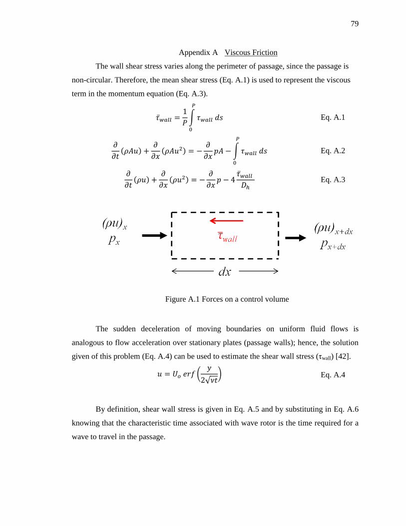
79

Appendix A Viscous Friction

The wall shear stress varies along the perimeter of passage, since the passage is

non-circular. Therefore, the mean shear stress (Eq. A.1) is used to represent the viscous

term in the momentum equation (Eq. A.3).

∫

Eq. A.1

( )

( )

∫

Eq. A.2

( )

( )

Eq. A.3

Figure A.1 Forces on a control volume

The sudden deceleration of moving boundaries on uniform fluid flows is

analogous to flow acceleration over stationary plates (passage walls); hence, the solution

given of this problem (Eq. A.4) can be used to estimate the shear wall stress (τwall) [42].

(

√ ) Eq. A.4

By definition, shear wall stress is given in Eq. A.5 and by substituting in Eq. A.6

knowing that the characteristic time associated with wave rotor is the time required for a

wave to travel in the passage.

80

|

|

Eq. A.5

√ √

Eq. A.6

The dimensionless form of the momentum equation is deduced by substitution of

the normalized conserved parameters given in Eq. A.7 which will lead to Eq. A.8, where

δ is length scale of the unsteady flow inside the passage representing the height of the

boundary layer [11].

Eq. A.7

( )

(

)

√ (

)

| | Eq. A.8

√

Eq. A.9

The skin friction can be represented in a generalized formula that is correlated to

Reynolds number and the geometry of the passage [8].

( ) (

)

(

)

Eq. A.10

By substituting the skin friction coefficient into the wall friction stress, the momentum

equation in its generalized form is given in Eq. A.11.

( )

(

)

| | Eq. A.11

(

)

(

) Eq. A.12

Eq. A.13

The power parameters have been calibrated with experimental data from the wave

rotor pressure exchanger rig that has been used by Paxson to validate the numerical

model for pressure exchanger topping cycles application and value of η = 0.25 is found to

81

give the best prediction with experimental data. The momentum equation in the non-

dimensional form is henceforth updated to the empirically validated form shown in Eq.

A.14

( )

(

)

| | Eq. A.14

82

Appendix B Heat Transfer

The heat transfer coefficient is calculated based up on the principle of analogy

between momentum and heat transfer first recognized by Reynolds. The average film

heat transfer coefficient has been solved by Pohlhaussen given in Eq. B.1 [43]. This

equation is simply translated into a correlation for Nusselt number as shown in Eq. B.2.

Eq. B.1

Eq. B.2

The Stanton number is deduced to be:

Eq. B.3

The average skin friction coefficient is defined as:

Eq. B.4

By substitution of Eq. B.3 in Eq. B.4 we get:

Eq. B.5

Hence the heat transfer coefficient is correlated to the skin friction coefficient and

consequently the shear stress term.

Eq. B.6

( )

( ) Eq. B.7

The non-dimensional form of the energy equation with the heat loss per unit cell is given

in Eq. B.8.

(

( )

∑

)

(

( )

∑

)

(

) (

) ( )|

|

Eq. B.8

83

The wall temperature is updated with a lumped capacitance model. Energy

storage in the control volume of passage walls is conserved to the total heat transfer

between the gas inside the passage (inner medium) and ambient air (outer medium) to the

passage walls.

Eq. B.9

( ) ( )

Eq. B.10

The convection heat transfer coefficient for the inner medium is typically as given

in Eq. B.10 with substitution of shear wall stress as with the generalized formulation of

the skin friction coefficient in Eq. B.5. The heat transfer coefficient for the outer medium

is derived from Colburn’s equation for steady turbulent flow over a plate such that the

plate length is equivalent to the unrolled outer circumference of the rotor. The flow speed

is analogous to the rotor tip speed.

The local Stanton number for such a problem is given in Eq. B.11 which is used

to estimate the heat transfer coefficient.

Eq. B.11

The rate of change of wall temperature is then deduced in the dimensionless form as

shown in Eq. B.12.

(

) (

) Eq. B.12

(

) (

) (

) | | Eq. B.13

(

) (

) (

) (

)

(

)

Eq. B.14

84

Appendix C Turbulence Eddy-Diffusivity

The control volume Figure C.1. is considered to formulate the net momentum

transported into the cell by turbulent diffusion

Figure C.1 Control volume unit cell of a passage

The transported momentum over the control volume is given in Eq. C.1.

( )

(

(

))

Eq. C.1

The turbulent viscosity coefficient can be modeled in terms of the eddy diffusivity and

the laminar viscosity coefficient as given in Eq. C.2.

Eq. C.2

By substituting the turbulent viscosity from Eq. A.30 in Eq. A.29 and normalization with

reference parameters, the momentum equation is updated with the turbulence term is

given in Eq. A.31.

( )

(

)

| | Eq. C.3

Total energy diffusion includes the kinetic, thermal and chemical energies

transported through the working fluids through the passage. Kinetic energy diffusion

through a control volume representing a unit cell from the passage is shown in Eq. C.4.

( )

(

) (

(

( )

))

( )

Eq. C.4

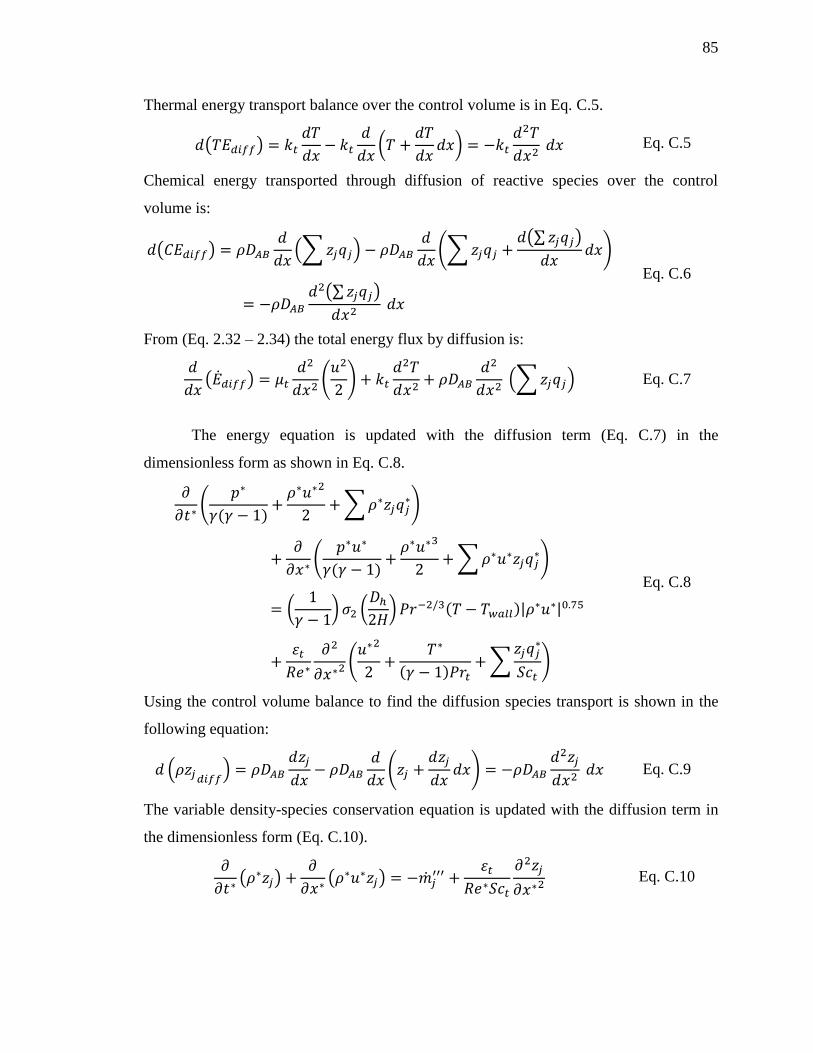
85

Thermal energy transport balance over the control volume is in Eq. C.5.

( )

(

)

Eq. C.5

Chemical energy transported through diffusion of reactive species over the control

volume is:

( )

(∑ )

(∑

(∑ )

)

(∑ )

Eq. C.6

From (Eq. 2.32 – 2.34) the total energy flux by diffusion is:

( )

(

)

(∑ ) Eq. C.7

The energy equation is updated with the diffusion term (Eq. C.7) in the

dimensionless form as shown in Eq. C.8.

(

( )

∑

)

(

( )

∑

)

(

) (

) ( )|

|

(

( ) ∑

)

Eq. C.8

Using the control volume balance to find the diffusion species transport is shown in the

following equation:

( )

(

)

Eq. C.9

The variable density-species conservation equation is updated with the diffusion term in

the dimensionless form (Eq. C.10).

( )

( )

Eq. C.10

86

Appendix D Boundary Conditions

The boundary conditions of the ports are set to be automatically distinguishing the

type of the flow (subsonic, sonic or supersonic) and its direction (inflow or outflow). The

conditions at point 0 are set to match the isentropic flow characteristics from the

upstream conditions (stagnation for inflow and static for outflow) with the half Riemann

problem solved between point 0 and 1.

The flow type and direction are based on the Mach number of the boundary cell

and the pressure ratio between the port and the boundary cells from which the

correlations can be specified by solving the isentropic flow equations as shown in Figure

D.1. The walls boundary conditions are simply specified by setting the velocity of the

imaginary cell to 0. Meanwhile, the pressure at the wall is estimated from the boundary

cell at the previous time step with the shock or the characteristic equations based on the

Mach number and pressure of the boundary cell.

Figure D.1 Boundary Port Flow Conditions [7]

87

Appendix E TVD Lax-Wendroff Scheme

The spatial domain of the WRCVC passage is discretized to a number of cells;

each cell size is equal to Δx, and the time domain is discretized with a time step equal to

Δt. The numerical solution aims to solve the conserved independent variables for each

cell at every time step.

The conserved vector w(x, t) is expanded in a Taylor series at a given time as

shown in (Eq. E.1) and rearranged such that the numerical derivative of w(x, t) with time

in (Eq. E.2) is the difference between properties at time step n and the next time step n+1

divided by the time step Δt. This numerical discretization for the first derivative of w(x, t)

is shown to be a second order of accuracy after the truncation of higher order terms in the

Taylor series [44].

(

) (

)

( ) Eq. E.1

(

) (

)

( ) Eq. E.2

Similarly the first derivative of the flux vector f(w, x) is approximated as follows:

( ) Eq. E.3

By adding Eq. A.39 and Eq. A.40 and subtracting source term Si we get a

numerical approximation for the differential equation (Eq. 2.43, see chapter 2) of second

order of accuracy in space and time:

(

) (

)

Eq. E.4

In order to maintain the second order of accuracy in time for the approximated

differential equation, a suitable approximation for the second order of derivative of the

conserved vector w(x, t) with time is required. The second derivative of the conserved

vector is approached by taking the derivative with respect to time for Eq. 2.43 as shown

in Eq. E.5. The coordinate transformation for the flux vector is shown in Eq. E.6 where

the Jacobian of the transformation is the derivative of flux vector with the conserved

vector noted as vector [A].

88

(

)

Eq. E.5

(

)

(

)

(

)

([ ]

) Eq. E.6

The first derivative of the conserved vector w(x, t) is known from Eq. 2.43. By

substitution into Eq. E.6 and thereafter all into Eq. E.5, the second derivative of w(x, t)

with time is expressed in terms of spatial derivatives of flux and source vectors.

([ ]

)

([ ] )

Eq. E.7

The double derivative term on the right hand side of Eq. E.7 is an anti-diffusive

term of second order of accuracy, and hence the limiters of the TVD scheme are applied

to the Lax-Wendroff’s approximation for this derivative [27].

([ ]

) [ ]

(

)

[ ]

(

)

Eq. E.8

Where the Jacobian at cell face is:

[ ]

[ ]

[ ]

Eq. E.9

The approximation of Eq. E.5 with backward time center spaced discretization is

presented in Eq. E.10.

([ ]

(

)

[ ]

(

)

)

([ ]

[ ]

)

(

)

( )

Eq. E.10

Rearrangement of the approximation of governing system can be presented in more

compact form as follows:

(

)

(

) Eq. E.11

The flux vector at cell face is:

89

[ ]

(

)

([ ]

[ ]

) Eq. E.12

Eq. E.13

The source of information required to solve for the conserved parameters in the

nest time step is shown in the schematic diagram (Figure E.1)

Figure E.1 Lax-Wendroff one-step method stencil [44]

90

Appendix F Approximate Riemann Solvers (The Method of Roe)

Roe’s algorithm for convective fluxes calculation, proposed that the Riemann

solution of any set of non-linear conservation laws can be tackled with a linearization

procedure for the non-linear terms. This approximation enhanced the computation

promptness compared to the exact solution procedures which involves iteration processes

that is most likely very expensive. The method averages a cell conditions through the

information coming from the left and right cells at the cell face fluxes with the

characteristic lines of waves with characteristic speed, vector and wave strength [7].

⟦( ) ∑ | | ∑ [ ( ) ] | | ⟧ Eq. F.1

The flux limiter is function of the ratio of successive gradients.

Eq. F.2

The limiter function is restricted to certain values in order to maintain the scheme

oscillatory free and second order of accuracy. This scheme produces the sharpest

resolution for discontinuities when the flux limiters are restricted to accuracy constraints.

The scheme for which the constraints on the flux limiters fulfilled is called “superbee”

scheme. The regions of limiters value for the superbee scheme shown in Figure F.1

(hatched)

Figure F.1 Superbee limiter bounds [7]

91

Appendix G Wave Strengths

According to Roe’s method of linearization, small perturbations about the mean

value of the primary variable of the conserved vector (p, ρ, and u) are assumed. The

conserved vector in this linearized form is,

[

]

Eq. G.1

Where the parameters with prime superscript represent the small perturbations

and the parameters with tilde are the mean value. The parameters of the linearized form

of the conserved vector are given as follows:

√ √

√ √

√

√ √

√ √

Eq. G.2

The wave strength is the product of the mean left eigenvectors (inverse of right

eigenvector – see section 3.3.) with the linearized conserved vector.

The wave strengths are:

92

2

2

2

2

2

2

~2

~~

~~~

~~~

~~~

~

~2

~~

a

uap

zza

p

zza

p

zza

p

a

pa

uap

ii

oo

ff

Eq. G.3

Graduate School ETD Form 9

Documents

Transcript of Graduate School ETD Form 9