Goodman 2017 - The Income Elasticity of Demand for Health ... 2017... · The Income Elasticity of...

The Income Elasticity of Demand for Health Insurance

Sarah Goodman

Supervisor: Jonathan Kolstad

University of California, Berkeley, Department of Economics

Spring 2017


2

Abstract

The level of national health expenditure as a percent of GDP has more than doubled since

1970 in OECD countries. Many health economists theorize that rising income causes the

increased health share of GDP. The goal of this paper is to estimate the national and global

income elasticity of demand for the health share of GDP, and to determine whether income is the

main driver of increased health share. OECD data is used to examine this question through

Ordinary Least Squares, Two Stage Least Squares, and Lasso regressions. The health share of

GDP is found to be income inelastic and non-zero with an income elasticity estimate of 0.4. This

suggests that national health expenditure is elastic, and relative increases in health expenditure

will continue to outpace the rate of rising income. Non-income, country-specific factors are more

important indicators of the health share of GDP.


3

1. Introduction

In the United States, health care expenditure as a share of GDP has greatly increased over

the last 50 years. In 1970, health care spending was only 6.2% of GDP; but by 2015 it had risen

to 16.9% of GDP. Similar trends have been seen in other developed countries. In France, the

share of GDP devoted to health care rose from 5.2% in 1970 to 11% in 2015. Japanese health

care spending was 4.4% of GDP in 1970, and 11.2% in 2015. The share of GDP going to health

expenditure more than doubled in most OECD countries from 1970-2014.

There are several theories for the increase in health expenditure. Technological change

and innovation are often cited as the causes of some of the increase, as demand for expensive

technologies to prolong life increases. Hall and Jones (2007) argue that increasing income will

always result in increased health expenditure because there are no diminishing returns to health

consumption. They base this argument on a model of an economy with two types of

consumption: health consumption and non-health consumption. Non-health consumption has

decreasing marginal returns in each period, they argue, and to increase lifetime utility one must

increase the number of periods in which they can consume –in other words, their life expectancy.

Health consumption will increase life expectancy and thereby lifetime utility. Non-health

consumption, on the other hand, has diminishing returns to period utility and therefore will not

increase lifetime utility. It follows that as income increases, non-health consumption will grow at

a slower rate than income, and health consumption will grow at a faster rate than income. Hall

and Jones (2007) predict that based on the undiminishing marginal utility of extending one’s life,

the optimal level of health care expenditure in the United States will exceed thirty percent of

GDP by the middle of the twenty-first century.


4

Another theory of increased health expenditure centers around the social value of

improvements in health – the gains in social welfare that result from improvements in health.

Murphy and Topel (2005) show that the social value of improvements in health are greater with

larger populations, higher average life incomes, greater existing levels of health, and closeness in

population age to the onset of disease. They conclude that as the U.S. population grows, lifetime

income increases, health levels improve, and the baby boom generation approaches the age of

disease-related death, the social improvements in health will continue to rise. This hypothesis

justifies the increases in health expenditure seen in recent decades, and suggests that health

expenditure will continue to grow at an equal or greater rate.

A study by Finkelstein et al. (2013) further examines the causal relationship between

rising incomes and health spending as a percent of GDP. The study uses the interaction of oil

prices and oil reserves to instrument for local area income effects in its causal relationship with

health spending. Finkelstein et al. finds that the income elasticity of demand is below unity, or in

other words, that rising incomes do not, in fact, explain the rising health share of GDP. However,

this study measures health expenditure through hospital expenditure instead of total health

expenditures, and aims to measure local area effects, not national or global ones. For these

reasons, a different income elasticity of demand may be found when estimating the effect of

rising national income on total health share of GDP.

In his 2007 paper, White compares the growth of health expenditure between the United

States and other OECD countries. He decomposes the growth in per capita health expenditure

into three components: real growth in per capita income, national annual population aging, and

“excess growth,” defined as real growth in health expenditure not attributable to the first two

categories. He finds that the United States had far more excess growth in health spending from


5

1970-2002 compared to OECD countries. White suggests that this trend is not due to high cost

technological improvements because technology flows freely between high income countries.

Instead, he argues, it is likely due to institutional factors such as the organization of health care

financing and delivery: namely, the fact that OECD countries give a central body – either the

national government or social insurance administrators – more authority to constrain health

spending than the United States.

This paper will examine three distinct models of national health care and determine

whether there is a relationship between health care model and health expenditure as a share of

GDP over time. Most cross-sectional time series studies have found an income elasticity of

demand at or around unity in developed countries (Hitris and Posnett; Hansen and King).

However, Hitris and Posnett (1992) suggest that parameters related to the financing and delivery

of health care may have direct or indirect effects on national demand for health care, and that

treating developed countries as a single homogenous group may be problematic. This study will

therefore analyze the relationship between health expenditure and GDP on a country-by-country,

as well as model-by-model basis.

The first model will be the Private Model, employed by only the United States. In this

model, health delivery is mostly private and is paid for in part by private insurance companies.

Individuals in turn pay these private insurance companies to receive health services.

Misleadingly, the United States “Private Model” is not entirely private. Medicare, Medicaid, and

the Veterans Health Administration may all be considered as some of the non-private elements of

the United States health care system. The U.S. underwent a large health care transition in 2010,

when the Patient Protection and Affordable Care Act (ACA) was passed. This law had multiple

components, including a mandate that all individuals obtain health insurance coverage or risk


6

paying a fine, and expansion of certain publically provided services, such as the proportion of the

population covered by Medicaid. However, even before the ACA, almost half of all health

spending was public, so the categorization of the U.S. as employing a “Private Model” is a

relative term used for the purposes of this paper.

The second model of study is the Beveridge model, which is funded publically through

taxation and centrally organized into a national health service of some type. Countries that

employ this model include the United Kingdom, Italy, Spain, Sweden, Denmark, Norway, and

Finland. Health services are publicly distributed through the same central organization. The

United Kingdom has been following the Beveridge model since the inception of the National

Health Service in 1948. The Italian National Healthcare Service was created in 1978 and is

inspired largely by the British system. Although Spain had some form of national health care

since the mid-1970s, they were considered a Bismarck model until their financial reorganization

in 1989, whence they switched to Beveridge. Sweden passed their National Health Insurance Act

in 1946 to fund health care through taxes, and Denmark moved to their National Health Security

System in 1973. Norway was extremely early, passing the Health Practitioners’ Act of 1912 to

guarantee all citizens equal access to physician services regardless of income, and finessing their

publically-funded care since then. The Finnish health care system has developed gradually as

well, and no exact year has been identified as the introduction of their tax-based system.

The final model of study will be the Bismarck model, found in Germany, France,

Switzerland, Japan, the Netherlands, and Belgium. The Bismarck model is often called a

“mixed” model because there is both private and public provision of care. Funding is public,

achieved through the compulsory health insurance premiums. Germany introduced mandatory

national health insurance in 1883, and the model’s namesake, Otto von Bismarck, proposed the


7

initial Health Insurance Bill of 1883. France instituted statutory health insurance as a part of the

social security system in 1945. In Switzerland, attempts to nationalize health care were made as

early as 1890, but strong centralization and reform were not successful until 1994. Japan

established national health insurance in 1961, but the Netherlands established mandatory

insurance in just 2006. In Belgium, health insurance was made compulsory for all salaried

workers in 1944.

Model Description Countries Private Private insurance,

private providers United States

Beveridge Public insurance, government-employed providers

United Kingdom Italy Spain Sweden Denmark Norway Finland

Bismarck Public insurance, private providers

Germany Japan Netherlands Belgium France (omitted) Switzerland (omitted)


8

2. Data Overview – Increasing Health Expenditures

This paper primarily uses data from Organization for Economic Cooperation and

Development (OECD) database from 1970-2014. As mentioned previously, this paper includes

data on the United States, Germany, Netherlands, United Kingdom, Japan, Italy, Spain, Sweden,

Finland, Norway, Denmark, and Belgium. The countries of Switzerland and France were omitted

from this study due to data constraints. The main outcome of interest is national health

expenditure, which measures the final consumption of health care goods and services, excluding

any spending on health care investments. National health expenditure is given as a percent of

annual GDP throughout the entirety of this paper.

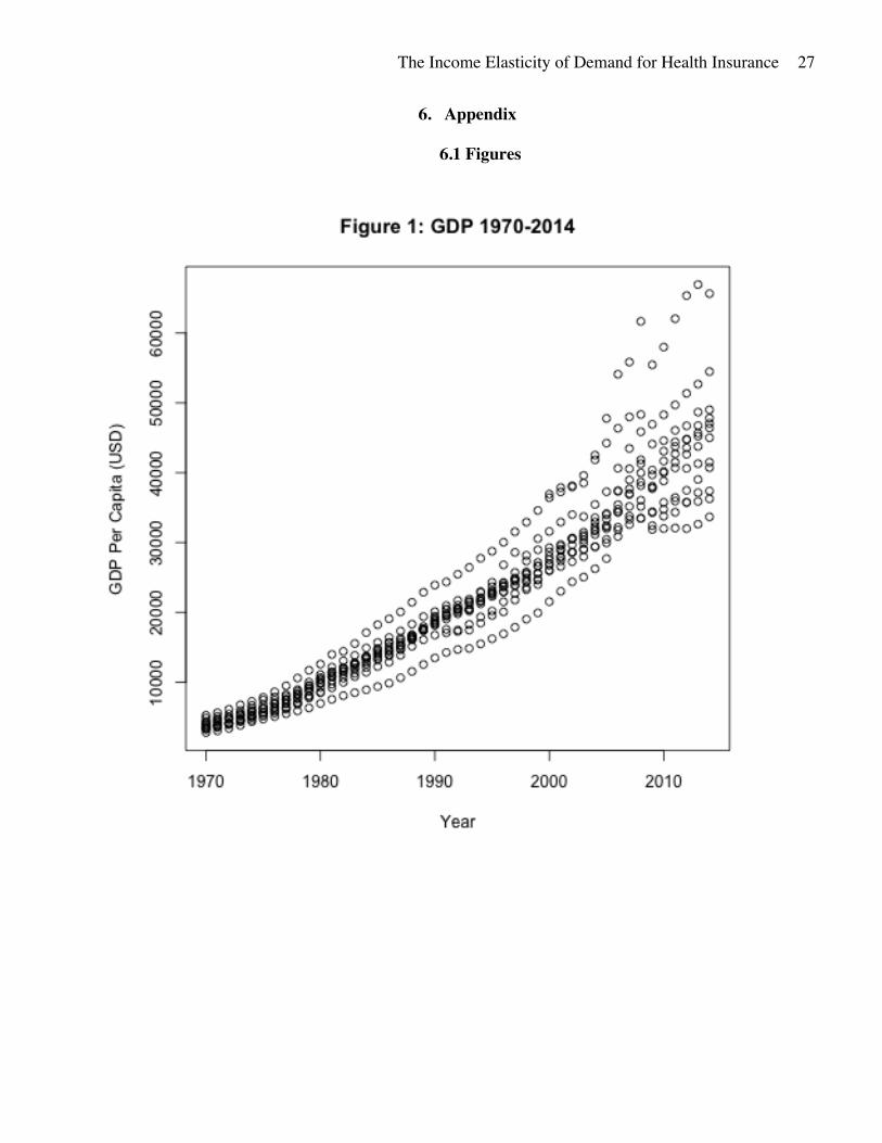
From 1970 to 2014, income per capita has increased steadily across the board. The average

increase in GDP per capita across all study countries was 987.8 USD from 1970-2014 (Figure 1).

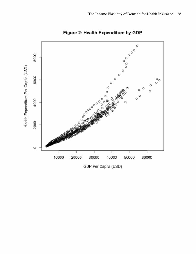
Health expenditure also increased over this period, an increase of 106.7 USD per capita. As may

be expected, there is a strong relationship between per capita health expenditure and GDP.

Richer countries tend to spend more on health care goods and services (Figure 2). This positive

correlation between GDP per capita and national health expenditure per capita is very clear in the

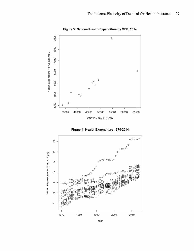
most recent data from 2014 (Figure 3).

However, the positive correlation between income and national health expenditure is not

sufficient to explain the increases in health expenditure; the growth in health expenditure has

exceeded the growth in GDP since 1970. Figure 4 shows that health expenditure as a percent of

GDP has continuously risen in all study countries 1970-2014. Although all countries have

experienced increases in health expenditure as a percent of GDP, the United States has shown

substantially more growth in this metric 1970-2014, as displayed in Figure 4 and Figure 5.


9

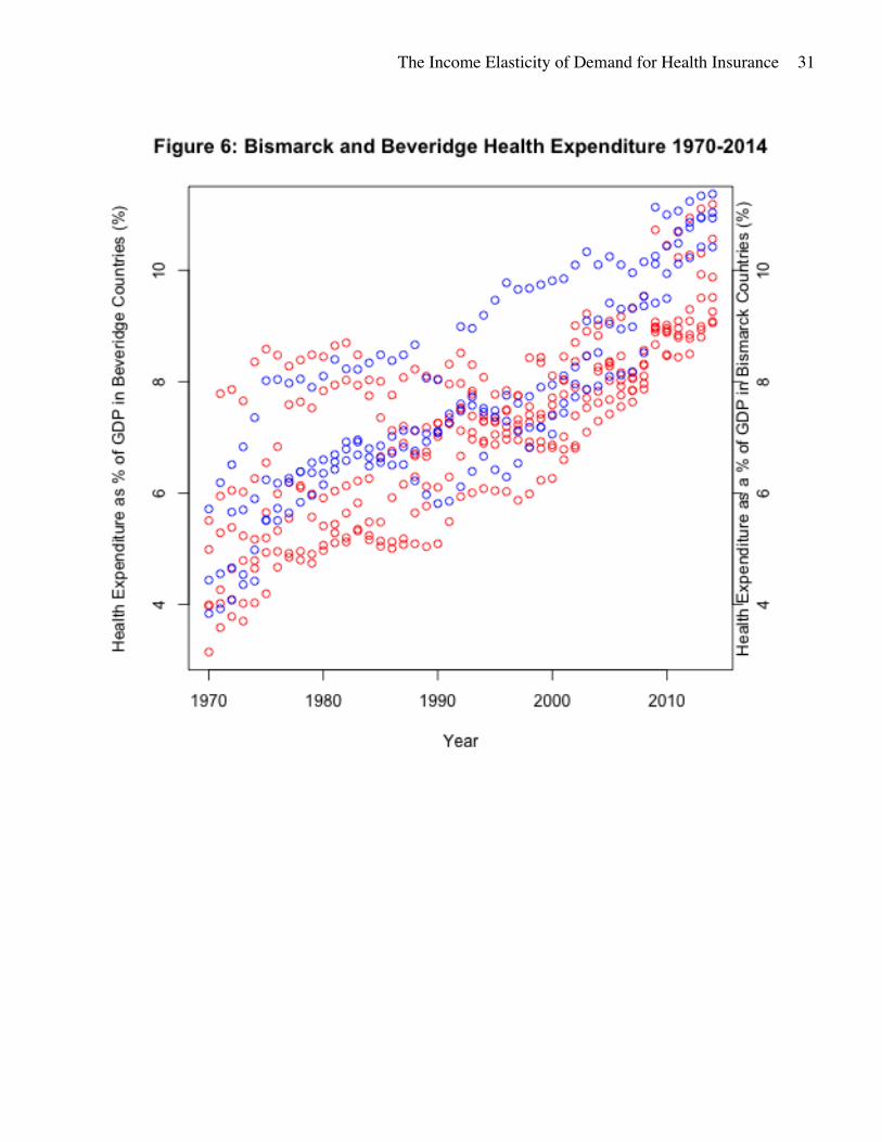
Figure 6 examine differences in health expenditure between Bismarck (blue) and Beveridge

(red) countries. Bismarck countries appear to have higher health spending on average, but the

growth in health spending appears to be approximately the same in both groups.

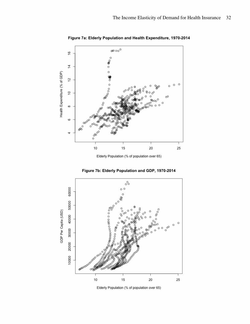
There are many nation-level factors affecting the relationship between GDP and health

expenditure. The demographic makeup of a country’s population may be related to both income

and spending on health. An important consideration is the average age of the population in a

country. Typically, people consume more health services in later stages of their life. In 2004, the

per capita health spending in the U.S. for males and females aged 65 and over was over three

times the average level of per capita health spending for those aged 19-64 (Cylus et al., 2011).

There is also a strong relationship between life expectancy and income, although the direction of

this relationship is debated (Servellati and Sunde, 2011; Lorentzen et al., 2008; Acemoglu and

Johnson, 2007). These two trends are also seen in the countries examined in this paper; the

relative size of the elderly population is associated with higher income levels and higher health

share of GDP (Figure 7a, Figure 7b). All three variables – health expenditure, GDP, and the

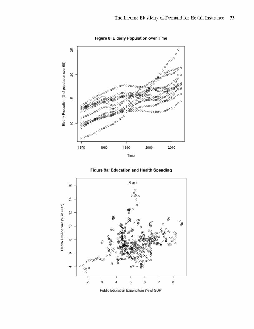
relative size of the elderly population – have increased from 1970-2014 in all study countries

(Figure 8).

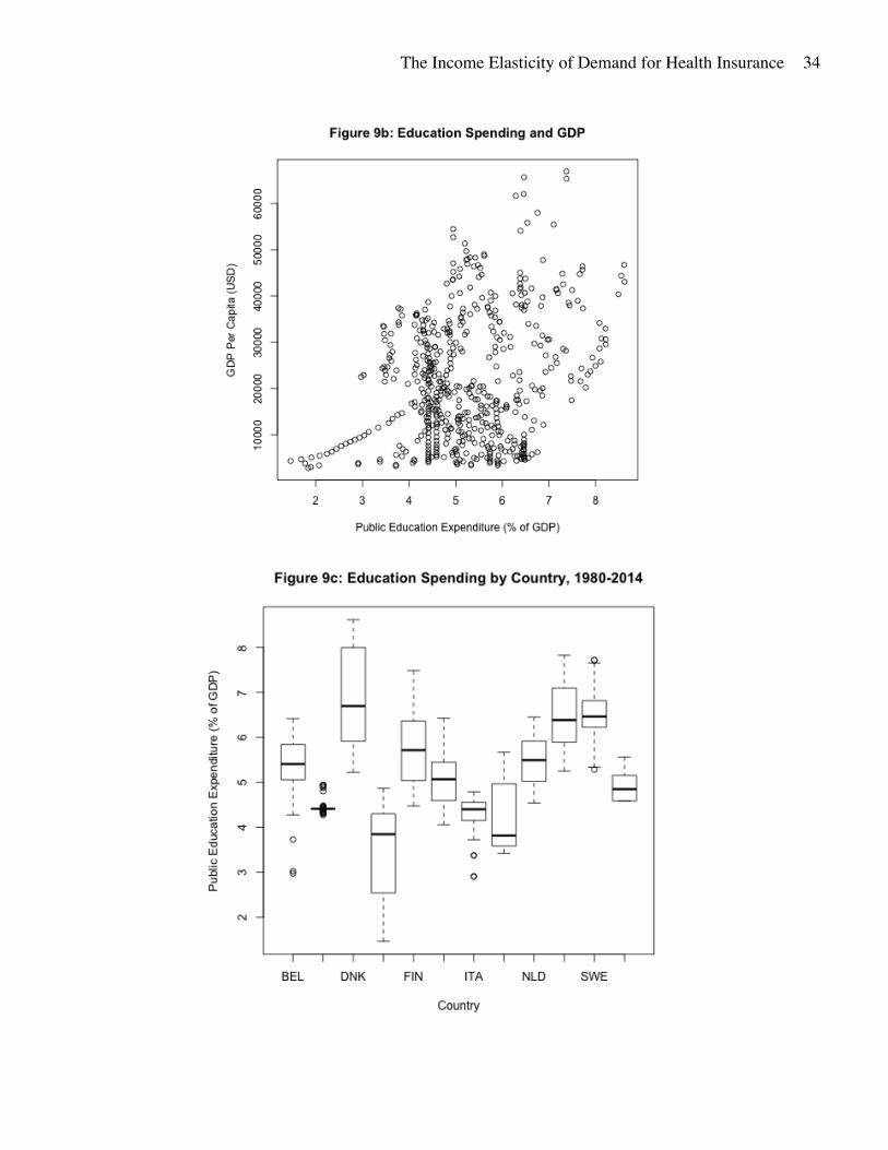
Another variable taken into consideration is public education spending. Education is a

publicly and privately provided good, just like health care. The share of income spent on public

education may be indicative of the value a country places on public goods and services. Health

expenditure and public education expenditure are positively correlated, as are GDP and public

education expenditure (Figure 9a and Figure 9b). The level of public education expenditure

varies by country, but generally rests between 3% and 7% of annual GDP (Figure 9c). The

average level of public education spending is consistent across health care models (Figure 9d).


10

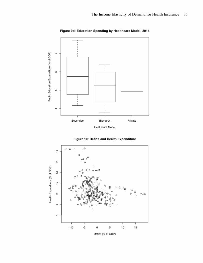
A country’s budget deficit or surplus as a percent of GDP was also considered in this paper.

Deficit or surplus indicates the amount of total government spending relative to national income:

a positive value represents annual government spending is less than the national income of the

country and a negative value represents government spending exceeds national income in that

year. A country’s annual deficit relative to national income may be related to the level of

national health expenditure relative to income (Figure 10). In particular, Norway and the United

States show signs that there may be a negative correlation between the level of government

surplus and health expenditure as a share of GDP. Norway has a consistently high surplus, and a

relatively low share of GDP spent on health care; from 1995 to 2014 Norway ran an average

surplus of 11% of GDP, and from 1970 to 2014 health expenditure was 7% of GDP. By contrast,

in 2014 the United States ran a deficit equal to 5% of GDP, and health expenditure was over

16% of GDP. Despite this evidence, deficit was not considered in the final regressions due to

data constraints.

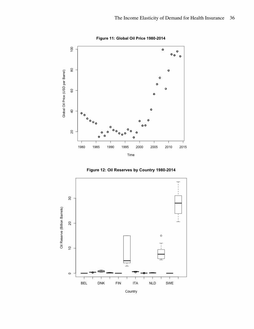
Following the study by Finkelstein et al., global oil price and national oil reserves are

included in the dataset. Oil prices gradually decreased 1980-1990 and remained fairly consistent

1990-2000, before increasing sharply 2000-2014 (Figure 11). National oil reserves vary by

country and year, but the United States consistently had the highest oil reserves during the study

period (Figure 12).


11

3. Results

The main goal of this paper is to discern any differences in the income elasticity of demand

for health share of GDP between Beveridge and Bismarck models. The income elasticity of

demand for health share will be taken as the coefficient on the natural log, or percent growth, of

GDP, the independent variable, when regressed on the natural log of health expenditure as a

percent of GDP. This estimate is represented as 𝛽"in equation 2.

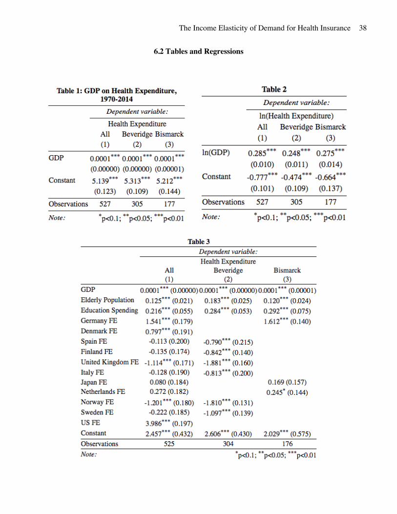
The preliminary regression (Table 1) shows again the positive relationship between GDP and

health expenditure as a percent of GDP, and that approximately the same relationship is seen in

both Bismarck and Beveridge countries. Table 1 shows the regression results of equation 1.

ℎ𝑒𝑎𝑙𝑡ℎ𝑒𝑥𝑝*+ = 𝛽- + 𝛽"𝑔𝑑𝑝*+ + 𝜀*+ (1)

[Table 1, page 38]

ln(ℎ𝑒𝑎𝑙𝑡ℎ𝑒𝑥𝑝*+) = 𝛽- + 𝛽"ln(𝑔𝑑𝑝*+) + 𝜀*+ (2)

Using equation 2, the baseline estimate of the income elasticity of demand is shown in Table

2. The baseline estimate excluding all other variable is an income elasticity around 0.29 for all

study countries, 0.25 for Beveridge countries, and 0.28 for Bismarck countries.

[Table 2, page 38]

3.1 Results: The Role of Education and the Elderly

Although these results appear very statistically significant, it is possible that they are a

result of country-level confounding factors. For this reason, it is important to include variables

for country fixed effects, and certain country-level covariates. The first covariate examined is the


12

elderly population, retrieved from the OECD website, and measured as the percent of the

population over 65. With a large population over 65, a country may face increased health costs

because individuals aged 65 and over are closer to the age of death and therefore statistically

more likely to consume life-lengthening and enhancing health goods and services. This

contributes to a potentially higher level of health expenditure as a percent of GDP.

The next covariate examined is education spending as a percent of GDP, retrieved from

the Urban Institute for Statistics. Health spending is potentially related to education spending

because both metrics may reveal a trend in the tendency of a country or its government to spend

on public goods.

ℎ𝑒𝑎𝑙𝑡ℎ𝑒𝑥𝑝*+ = 𝛽- + 𝛽"𝑔𝑑𝑝*+ + 𝛽7𝑒𝑙𝑑𝑙𝑦𝑝𝑜𝑝*+ +𝛽:𝑒𝑑𝑢𝑐*+ + 𝛾* + 𝜀*+ (3)

In regression 3, 𝑒𝑙𝑑𝑙𝑦𝑝𝑜𝑝*+ represents the percentage of the population over 65 in country

i during year t. The variable 𝑒𝑑𝑢𝑐*+ represents the percent of GDP spent by the government on

education in country i during year t. The variable 𝛾* is a set of country indicators, used to capture

the country fixed effects relative to the health expenditure found in Belgium.

[Table 3, page 38]

The regression results displayed in Table 3 show that GDP still has a positive relationship

with health expenditure. The coefficient of 0.0001 on GDP can be interpreted as an increase of 1

USD in per capita income is related to an increase of 0.0001 in the percent of GDP spent on

health care, on average. Elderly population also has a positive relationship with health


13

expenditure in all study countries, with a one percent increase in the population over 65 related

to an increase of 0.122 in the percent of GDP going to health expenditures. Education spending

is positively correlated with health expenditures as well – a one percent increase in the percent of

income spent on education is related to a 0.215 increase in health spending as a percent of GDP,

averaging across all study countries. All three relationships are significant at the one percent

level, and are seen when countries are separated into their respective Bismarck or Beveridge

groups as well.

Relative to the level of health expenditure in Belgium, Regression 3 shows that Germany,

Denmark, and the United States all spend significantly more on health when accounting for

variation in GDP, the elderly population, and education spending. In contrast, the United

Kingdom and Norway both spend significantly less. Out of all the coefficients, the United States

has the greatest magnitude, suggesting that when controlling for differences in GDP, education

spending, and the elderly population, the United States still has a far higher level of health

spending than other countries.

3.2 Results: Shocks and Instrumental Variables

Another important consideration in determining the relationship between health

expenditure and GDP is the deviations or shocks to either metric. Health expenditure shocks may

be caused by a sudden change in the organization of a country’s health system, or a new

government-provided health service with a large target population. Sudden changes in GDP may

be caused by a recession or a spike in global oil prices, if oil is a big part of the national

economy.


14

To account for this, health expenditure is smoothed over five year periods by taking a

moving average of health expenditure in each country. Exogenous GDP shocks are considered

by adding a variable for the annual global crude oil price, given in USD per barrel. Each

country’s economy relies to a different degree on oil, and therefore has a different level of

sensitivity to changes in oil price. National oil reserves are used to measure this sensitivity, given

in billions of barrels. An interaction variable for oil reserves and the price of oil is created is also

added to the regression. The oil price data is from Federal Reserve Economic Data (FRED), and

oil reserves are from the U.S. Energy Information Administration.

ℎ𝑒𝑎𝑙𝑡ℎ𝑒𝑥𝑝*+ = 𝛽- + 𝛽"𝑔𝑑𝑝*+ + 𝛽7𝑒𝑙𝑑𝑙𝑦𝑝𝑜𝑝*+ +𝛽:𝑒𝑑𝑢𝑐*+ + 𝛽>𝑜𝑖𝑙𝑝𝑟𝑖𝑐𝑒+ + 𝛽A𝑜𝑖𝑙𝑟𝑒𝑠𝑒𝑟𝑣𝑒𝑠*+ +

𝛽D𝑜𝑖𝑙𝑝𝑟𝑖𝑐𝑒+ ∗ 𝑜𝑖𝑙𝑟𝑒𝑠𝑒𝑟𝑣𝑒𝑠*+ + 𝛾* + 𝜀*+ (4)

The results for Regression 4 are displayed in Table 4.

[Table 4, page 39]

Table 4 reveals that smoothing health expenditure and adding oil prices does not change

the direction of the correlation between GDP and health expenditure, but does weaken the

magnitude of the relationship. The lower magnitude of the coefficient on GDP suggests that

health expenditure and GDP spikes occur at the same period, or that exogenous factors such as

oil price or oil reserves are mediating the relationship between health expenditure and GDP.

To determine whether the latter statement is valid, the interaction of oil price change and

oil reserves is used as an instrument on GDP growth in a two-stage least squares regression


15

(TSLS). Oil price change and GDP growth are both given as a whole number percent. Using an

instrumental variable on GDP growth will indicate whether increases in income cause increases

in the health share of GDP. As global oil prices increase, countries with larger oil reserves should

experience income growth. This is tested by the first stage of the TSLS, equation 5. If oil is

determined to be a relevant instrument for GDP growth, the second stage of the regression can be

used to determine whether exogenous GDP effects drive any changes in health expenditure. The

interaction of oil price and oil reserves is an exogenous instrument; it is unlikely that health

expenditure will affect either oil prices or oil reserves. For the sake of this study the exclusion

restriction is assumed to hold – oil price and oil reserves do not affect health expenditure through

any avenue besides GDP. However, the exclusion restriction cannot be guaranteed and thus oil

may be an invalid instrument if it affects health expenditure through another factor.

1st stage:

𝑔𝑑𝑝𝑔𝑟𝑜𝑤𝑡ℎ*+ = 𝜋- + 𝜋"𝑜𝑖𝑙𝑝𝑟𝑖𝑐𝑒𝑐ℎ𝑎𝑛𝑔𝑒+ ∗ 𝑜𝑖𝑙𝑟𝑒𝑠𝑒𝑟𝑣𝑒𝑠*+ + 𝜋7𝑋*+ + 𝜀*+ (5)

2nd stage

ℎ𝑒𝑎𝑙𝑡ℎ𝑒𝑥𝑝*+ = 𝛽- + 𝛽"𝑔𝑑𝑝𝑔𝑟𝑜𝑤𝑡ℎ*+ + 𝛽7𝑋*+ + 𝜀*+ (6)

Where 𝑋*+ represents all other covariates. The regression results from the first stage are

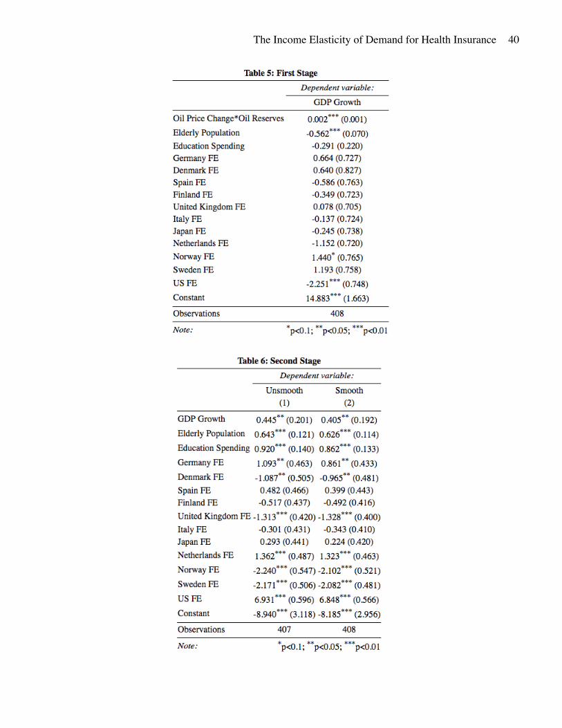
displayed in Table 5.

[Table 5, page 40]


16

Table 5 shows that the oil interaction variable is just relevant enough to be the instrument

for GDP growth and the TSLS may proceed to the second stage. The results of the second stage

are displayed in Table 6.

[Table 6, page 40]

The results from Table 6 show that GDP growth is a significant and positive driver of

health expenditure. An increase of 1% in per capita income causes the health share of GDP to

increase by 0.4 on average. The elderly share of the population is also positively correlated with

health expenditure. On average, a 1% increase in the percent of the population over 65 is related

to a 0.6 increase in health expenditure as a percent of GDP. When public spending on education

as a percent of GDP increases by 1, the average health share of GDP is higher by 0.9. Many

countries also see their own significant fixed effects. Germany, the Netherlands, and the United

States all spend significantly more on health care than Belgium after accounting for the

explained variation from GDP growth, the elderly population, and education spending. On the

other hand, Denmark, the UK, Norway, and Sweden all have a significantly smaller share of

GDP going to health care relative to Belgium after accounting for variation attributable to other

covariates. The United States has the highest level of health expenditure by far – its fixed effects

coefficient is over three times the magnitude of any other coefficient. In general, the magnitude

of the significant coefficients for country fixed effects are much greater than the other covariate

coefficients, particularly GDP growth. Health expenditure is therefore largely associated with

certain country-specific factors not included in this study.


17

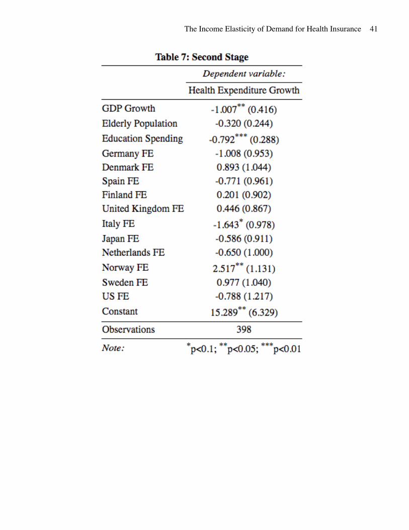
3.3 Results: Income Elasticity using Instrumental Variables

To obtain an estimate for the income elasticity of demand for health share of GDP,

another TSLS is run using equation 5 as the first stage and equation 7 as the second stage. In

equation 7, 𝛽"represents the central estimate for the income elasticity of demand.

1st stage:

𝑔𝑑𝑝𝑔𝑟𝑜𝑤𝑡ℎ*+ = 𝜋- + 𝜋"𝑜𝑖𝑙𝑝𝑟𝑖𝑐𝑒𝑐ℎ𝑎𝑛𝑔𝑒+ ∗ 𝑜𝑖𝑙𝑟𝑒𝑠𝑒𝑟𝑣𝑒𝑠*+ + 𝜋7𝑋*+ + 𝜀*+ (5)

2nd stage

ℎ𝑒𝑎𝑙𝑡ℎ𝑒𝑥𝑝𝑔𝑟𝑜𝑤𝑡ℎ*+ = 𝛽- + 𝛽"𝑔𝑑𝑝𝑔𝑟𝑜𝑤𝑡ℎ*+ + 𝛽7𝑋*+ + 𝜀*+ (7)

With oil price change, health expenditure growth, and GDP growth given as a whole

number percent. The results from equation 7 are displayed in Table 7.

[Table 7, page 41]

The coefficient on GDP growth shows that a 1% increase in annual GDP causes a 1%

decrease in the health share of GDP. This estimate may be due to health expenditure having a

lagged response to increases in GDP. Health expenditure is given as a portion of GDP, and if the

level of health spending stays constant while GDP grows, then health expenditure as a percent of

GDP will decrease. Therefore, a lagged value of GDP growth must be used as the endogenous

regressor in order to accurately capture the effects of GDP growth on the growth of health share

of GDP. The new TSLS equations using lagged GDP growth and lagged oil interaction are

shown in equations 8 and 9.


18

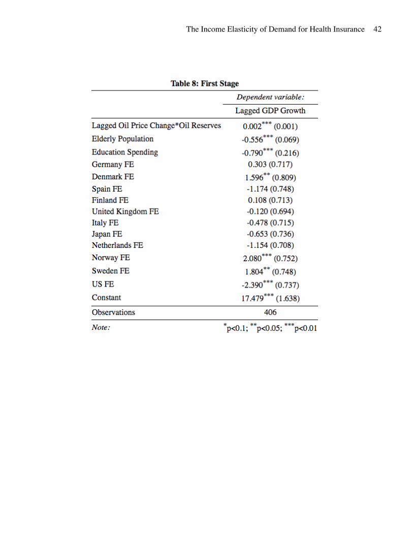
1st stage:

𝑔𝑑𝑝𝑔𝑟𝑜𝑤𝑡ℎ*(+J") = 𝜋- + 𝜋"𝑜𝑖𝑙𝑝𝑟𝑖𝑐𝑒𝑐ℎ𝑎𝑛𝑔𝑒+J" ∗ 𝑜𝑖𝑙𝑟𝑒𝑠𝑒𝑟𝑣𝑒𝑠*+J" + 𝜋7𝑋*+ + 𝜀*+ (8)

2nd stage

ℎ𝑒𝑎𝑙𝑡ℎ𝑒𝑥𝑝𝑔𝑟𝑜𝑤𝑡ℎ*+ = 𝛽- + 𝛽"𝑔𝑑𝑝𝑔𝑟𝑜𝑤𝑡ℎ*(+J") + 𝛽7𝑋*+ + 𝜀*+ (9)

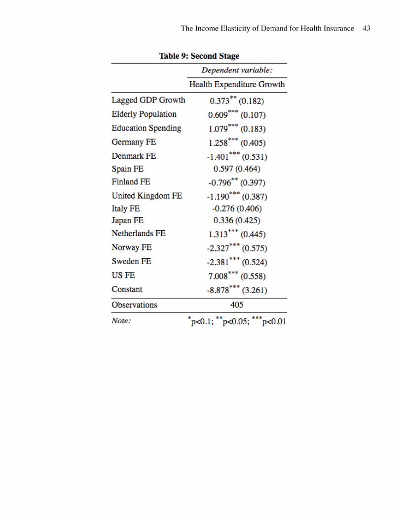
The results of equation 8 are shown in Table 8. Oil was again found to be a relevant

instrument, and the second stage results are shown in Table 9.

[Table 8, page 42]

[Table 9, page 43]

The central estimate of 𝛽", the estimated income elasticity of demand for health share of

GDP, is found to be 0.373 and significant at the 5% level. As GDP grows, the health share of

GDP also grows – a 1% increase in per capita income causes on average a 0.373% increase in

the health share of GDP.

There are significant limitations to understand when interpreting these regression results.

Firstly, there are considerations for oil prices and oil reserves. The interaction of oil price and oil

reserves was relevant, but not a very strong instrument. This may be due to the low oil reserve

levels of many countries in this study (Figure 12). Several countries have zero or near zero oil

reserves; in these countries oil is not a large part of the national economy and therefore oil price

changes do not greatly affect GDP growth. Secondly, the sizes of the country fixed effects

coefficients are larger than the estimated effect of GDP growth. Again, this suggest that health


19

expenditure is largely associated with certain country-specific factors not included in this study

that may be confounding any of the estimated relationships. Another consideration is the

construction of the growth variables – instead of using the natural log, a whole number percent

was used to capture growth. Thus, the estimate 𝛽" ~ 0.4 may be interpreted as a 1% increase in

YoY GDP causes an increase of 0.4% in the YoY health share of GDP.

Unfortunately, due to data constraints the income elasticity of health share could not be

calculated separately for the Beveridge, Bismarck, and Private models. With fewer observations

in each category the first stage regression was not relevant enough.

3.4 Results: Lasso Regression

An important risk of the above regressions is that the hypothesized models may be

overfitting the relationship of GDP and health spending. To discourage an over-fitted model, a

penalized regression must be used. A penalized regression minimizes error – the sum of squared

residuals – while creating a penalty for model complexity. This is a useful technique to prevent

overfitting when the exogenous regressors may be correlated with one another. The Lasso

method was determined to be the best type of penalized regression to employ based on the

sample constraints. Lasso employs the L1 norm, given as:

𝐿" = 𝛽- + 𝛽" + 𝛽7 +⋯+ 𝛽M < 𝑐 (6)

Where 𝛽* is the coefficient on variable i for a regression with n covariates. A lasso

regression minimizes the sum of squared residuals subject to the constraint that L1 is less than

some fixed value, c. Lasso shrinks all coefficients in the regression by some amount, lambda, 𝜆.


20

If a coefficient has a magnitude that is less than 𝜆, it becomes 0. Stricter Lasso regressions use a

high value of 𝜆 and return few non-zero coefficients. A Lasso regression with 𝜆 = 0 will be

indistinguishable from its non-penalized counterpart; all variables and their coefficients will be

included in the regression. Figure 13 displays a plot of all coefficients from the regression results

of equation 4 by decreasing 𝜆 value, for the range 𝜆 = [10-, 10J"-]. The six largest coefficients

are labeled to the right.

[Figure 13, page 37]

This figure shows that when all variables considered in this study are employed in an

Ordinary Least Squares regression, the country fixed effects for the United States have the

greatest effect on health expenditure as a percent of GDP. The United States has a level of health

expenditure that is higher than the variation explained by GDP, the elderly population, education

spending, oil reserves, etc. Furthermore, it is noteworthy that the next four largest drivers of

health spending are also country fixed effects for Germany, Norway, Sweden, and Spain, in

order. Germany and Spain have health expenditure exceeding the variation explained by other

covariates, including healthcare model. Norway and Sweden spend less on healthcare as a share

of GDP than the expected variation due to other factors. These results suggest that deviations in

the health share of GDP are explained by some set of country-level factors not included in the

above regression. The largest driver of health expenditure excluding all country fixed effects was

education spending, whose coefficient was the sixth largest in magnitude. Education spending

has a positive relationship with health expenditure, indicating that countries with a higher annual

public spending on education as a share of GDP also had higher health expenditure as a share of

GDP, on average.


21

An important limitation of the Lasso method in the context of this study is that it uses a

constant shrinkage value, or 𝜆 on all coefficients. This method favors variables with large

coefficients, which may not necessarily be the most important drivers of health expenditure. A

variable that is statistically significant but with a relatively small coefficient value may be

discounted even though it is an important factor in explaining variation in health expenditure.

For example, GDP has a very small coefficient but is significantly correlated with health

expenditure in the OLS regression, yet is not determined to be one of the most important drivers

of health expenditure using the Lasso method.

4. Conclusion

This paper finds that national health care expenditure is income elastic. The central

estimate for income elasticity of demand for the health share of GDP was approximately 0.4,

making health share of GDP income inelastic. An annual income increase of 1% is associated

with a 0.4% increase in the health share of GDP, or in other words an increase in health

expenditure exceeding the increase the respective increase in income by 40%, on average. This

suggests that the share of income going to health will continue rising with increasing global

income. The relative value of health increases with GDP and health is therefore a luxury good

when considered on a national scale.

However, these study results point to some exogenous, country-level factor as the most

significant in determining the national level of health share of GDP, one not captured by the

variation in the percent of the population that is elderly, public spending on education, or GDP.

This country-level factor appears to be strongest in the United States. These effects may have

been overestimated by using a year-over-year national growth percentage instead of the more


22

common natural log of income. Public education share of GDP was also significantly correlated

with health share of GDP, but there is uncertainty in the direction of this relationship.

Limitations of this study include the inability to capture such country-level factors, and

the lack of countries with health systems falling neatly into the private, Beveridge, and Bismarck

categories. The latter factor creates an inability to establish model-level trends that are

differentiable from the country-level trends. A possible expansion on this study that may indicate

model-level trends in health expenditure would be creating a database of countries that have

undergone a change in health care model, and measuring any differences before and after such

transition. Other future studies may seek out a stronger instrumental variable for GDP growth,

some exogenous measure that is more representative of the national economies.


23

5. Citations

Acemoglu, D., Finkelstein, A., & Notowidigdo, M. J. (2013). Income and health spending:

Evidence from oil price shocks. Review of Economics and Statistics, 95(4), 1079-1095.

Acemoglu, D., & Johnson, S. (2007). Disease and development: the effect of life expectancy on

economic growth. Journal of political Economy, 115(6), 925-985.

Busse, R., & Riesberg, A. (2004). Health care systems in transition: Germany. In Health care

systems in transition: Germany.

Cervellati, M., & Sunde, U. (2011). Life expectancy and economic growth: the role of the

demographic transition. Journal of economic growth, 16(2), 99-133.

Chen, A., & Goldman, D. (2016). Health Care Spending: Historical Trends and New

Directions. Annual Review of Economics, 8, 291-319.

Chetty, R., Stepner, M., Abraham, S., Lin, S., Scuderi, B., Turner, N., ... & Cutler, D. (2016).

The association between income and life expectancy in the United States, 2001-

2014. Jama, 315(16), 1750-1766.

Costa, D. L. (2015). Health and the Economy in the United States from 1750 to the

Present. Journal of economic literature, 53(3), 503-570.

Cylus, J., Hartman, M., Washington, B., Andrews, K., & Catlin, A. (2011). Pronounced gender

and age differences are evident in personal health care spending per person. Health

Affairs, 30(1), 153-160.

Docteur, E., & Oxley, H. (2003). Health-care systems: lessons from the reform experience.

Donatini, A., Rico, A., D'Ambrosio, M. G., Lo Scalzo, A., Orzella, L., Cicchetti, A., ... & World

Health Organization. (2001). Health care systems in transition: Italy.


24

Exter, A. D., Hermans, H., Dosljak, M., Busse, R., Ginneken, E. V., Schreyoegg, J., ... & World

Health Organization. (2004). Health care systems in transition: Netherlands.

FRED (2017). Crude Oil Prices: West Texas Intermediate (WTI) – Cushing, Oklahoma.

Available at https://fred.stlouisfed.org/series/DCOILWTICO

Furuholmen, C., & Magnussen, J. (2000). Health care systems in transition:

Norway. Copenhagen: WHO. European Observatory on Health Systems and Policies.

Hall, R. E., & Jones, C. I. (2004). The value of life and the rise in health spending (No. w10737).

National Bureau of Economic Research.

Hansen, P., & King, A. (1996). The determinants of health care expenditure: a cointegration

approach. Journal of health economics, 15(1), 127-137.

Hitiris, T., & Posnett, J. (1992). The determinants and effects of health expenditure in developed

countries. Journal of health economics, 11(2), 173-181.

James, G., Witten, D., Hastie, T., & Tibshirani, R. (2013). An introduction to statistical

learning (Vol. 6). New York: springer.

Järvelin, J. (2002). Health care systems in transition: Finland.

Lameire, N., Joffe, P., & Wiedemann, M. (1999). Healthcare systems—an international review:

an overview. Nephrology Dialysis Transplantation, 14(suppl 6), 3-9.

Lorentzen, P., McMillan, J., & Wacziarg, R. (2008). Death and development. Journal of

Economic Growth, 13(2), 81-124.

Maarse, H. (2006). The privatization of health care in Europe: an eight-country analysis. Journal

of Health Politics, Policy and Law, 31(5), 981-1014.

Meara, E., White, C., & Cutler, D. M. (2004). Trends in medical spending by age, 1963–

2000. Health Affairs, 23(4), 176-183.


25

Minder, A., Schoenholzer, H., & Amiet, M. (2000). Health Care Systems in Transition–

Switzerland.

Murphy, K. M., & Topel, R. H. (2006). The value of health and longevity. Journal of political

Economy, 114(5), 871-904.

OECD Data (2015). Health Spending. Available from https://data.oecd.org/healthres/health-

spending.htm

OECD Data (2016). Gross Domestic Product (GDP). Available from

https://data.oecd.org/gdp/gross-domestic-product-gdp.htm

OECD Data (2015). Elderly Population. Available from https://data.oecd.org/pop/elderly-

population.htm

OECD Data (2016). General Government Deficit. Available from

https://data.oecd.org/gga/general-government-deficit.htm

Rico, A. (2000). Health care systems in transition: Spain.

Sandier, S., Paris, V., Polton, D., Thomson, S., Mossialos, E., & World Health Organization.

(2004). Health care systems in transition: France.

Urban Institute for Statistics (2016). Education: Expenditure on Education as % of GDP (from

government sources). Retrieved from http://data.uis.unesco.org/?queryid=181

US EIA (2014). International Energy Statistics. Retrieved from

https://www.eia.gov/beta/international/data/browser/#/?vs=INTL.44-1-AFRC-

QBTU.A&vo=0&v=H&start=1980&end=2014

Verbelen, B. (2007). The impact of public expenditures on health care on total health

expenditures: An exploratory analysis of selected OECD countries. University of

Southern California.


26

White, C. (2007). Health care spending growth: how different is the United States from the rest

of the OECD?. Health Affairs, 26(1), 154-161.


27

6. Appendix

6.1 Figures


28


29


30


31


32


33


34


35


36


37


38

6.2 Tables and Regressions


39


40


41


42


43

Goodman 2017 - The Income Elasticity of Demand for Health ... 2017... · The Income Elasticity of...

Documents

Transcript of Goodman 2017 - The Income Elasticity of Demand for Health ... 2017... · The Income Elasticity of...