OXFORD lNSTITUl€

E N E R G Y STU D I ES

= FOR-

Are Price and Income Elasticities of Demand

Constant?

J. M. Dargay

Oxford Institute for Energy Studies

EE16

1992

ARE PRICE AND INCOME ELASTICITIES OF DEMAND CONSTANT?

THE UK EXPERIENCE J M DARGAY

EE16 OXFORD INSTITUTE FOR ENERGY STUDIES

The contents of this paper are the author’s sole responsibility.

They do not necessarily represent the views of the Oxford Institute for

Energy Studies or any of its Members.

Copyright 0 1992

Oxford Institute for Energy Studies Registered Charity, No: 286084

All rights reserved No pari of this publication may be reproduced, stored in a retrieval s y s m , or transmitted in any form or by any means. electrook, rnechanid photocopying, r e d i g . or otherwise, without prior permission of the Oxford Institute for Energy Studies.

lhis plblication is sold subject to the condition that it shall nol, by way of trade or &wise. be lent, resold, hired out. or otberwiae circulated without the publisher’s prior msent in any form of binding or cover other lhan that in which it is plblished and witbout a similar condition including this condition being imposed on the subsequent purchaser.

ISBN 0 948061 70 7

TABLES

1. Total Energy Consumption. Estimated Coefficients and Probability Values for Statistical Tests. Estimation Period 1961 to 1990. . . . . . . . . . . . . . . . . . . . . . . . . . . . . . . . . . . . . . . . . . . . . . . 24

2. Estimated Price and Income Elasticities. . . . . . . . . . . . . . . . . . . . . . . . . . . . . 26

3. Tests for the Specification of the Income Elasticity . . . . . . . . . . . . . . . . . . . . 29

4, Tests for Price Specifications for Constant (C) and Declining (D) Elasticity Models. Probability Values for F- or t-tests of H,, . . . . . . . . . . . . . . . . . . . . . . . . . . . . . . . . . . . . . . . . . . . 30

CONTENTS

1 . Introduction . . . . . . . . . . . . . . . . . . . . . . . . . . . . . . . . . . . . . . . . . . . . . . . . 1

2 . Total Energy Consumption . . . . . . . . . . . . . . . . . . . . . . . . . . . . . . . . . . . . . . 5

2.1 Measurement Issues . . . . . . . . . . . . . . . . . . . . . . . . . . . . . . . . . . . . . . 5

2.2 The Energy-GDP Ratio . . . . . . . . . . . . . . . . . . . . . . . . . . . . . . . . . . . 9

3 . Demand Specification and Hypothesis Testing . . . . . . . . . . . . . . . . . . . . . . . 15

3.1 Specification of the Income Elasticity . . . . . . . . . . . . . . . . . . . . . . . . 16

3.2 The Price Elasticity . . . . . . . . . . . . . . . . . . . . . . . . . . . . . . . . . . . . . 17

3.3 The Dynamic Adjustment Process . . . . . . . . . . . . . . . . . . . . . . . . . . . 21

4 . The Empirical Results . . . . . . . . . . . . . . . . . . . . . . . . . . . . . . . . . . . . . . . . 23

4.1 The Selected Models . . . . . . . . . . . . . . . . . . . . . . . . . . . . . . . . . . . . . . . . . 23

4.2 Price and Income Elasticities . . . . . . . . . . . . . . . . . . . . . . . . . . . . . . 26

4.3 Tests Concerning the Specification of

the Income Elasticity . . . . . . . . . . . . . . . . . . . . . . . . . . . . . . . . . . . . 29

4.4 Tests for Price Reversibility . . . . . . . . . . . . . . . . . . . . . . . . . . . . . . . 30

5 Conclusions . . . . . . . . . . . . . . . . . . . . . . . . . . . . . . . . . . . . . . . . . . . . . . . 33

References . . . . . . . . . . . . . . . . . . . . . . . . . . . . . . . . . . . . . . . . . . . . . . . . 37

1 INTRODUCTION

The reductions in energy demand witnessed since the oil price shocks of the 1970s have lent

undeniable evidence to the importance of prices in determining energy demand. Attempts to

actually measure the influence of prices on the basis of econometric models, however, have

resulted in a wide range of elasticities. Apart from differences in estimates based on international

cross-section data and times-series observations for individud countries, elasticities were often

found to be sensitive to the observation period used in the analysis.’ Just as elasticities based

on pre-1974 data could not explain the response to the energy price increases of the seventies,

estimates based on data including the high price era failed to explain the continued sluggish

growth in demand as prices began to fall in the mid-eighties. Estimates based on more recent data

began to suggest a lower elasticity than previous experience led us to believe, but the uncertainty

of the estimates grew, rather than diminished, as more recent data became available. Had the

price elasticity actually changed or had the models simply been unable to capture it?

This study addresses the question by re-examining aggregate energy demand in the UK for the

relatively long period from 1960 to 1990, giving three rather different energy price regimes: the

stable period of the sixties, high price era of the seventies and early eighties and the recent IOW

price era triggered by the price coIlapse of 1986. Our starting point is to challenge two of the

common assumptions made in the majority of energy demand studies: the existence of an

unchanging long-run demand relationship which is perfectly reversible to price changes and the

constancy of the income or GDP elasticity. The f i s t assumption basically implies that prices,

although influencing long-run demand, do not ‘shift’ the demand relationships themselves: that

is, despite all of the changes in the energy system made during the seventies and eighties in

response to high energy prices, a return to low energy prices - as is now the case - would

eventually restore demand to what it would have been had prices never risen. All that had been

done, would now be undone. Not only does this not seem to be happening, but it dso appears

To take a few estimates of the long-run price elasticity for the UK: Mittelstadt (1983) and Kouris (1980) find an elasticity of -0.4 for data up to 1978, Welsch (1989) finds an elasticity of -0.1 for 1960-84 and Hunt and Manning (1989) -0.3 for 1969-86.

0.1. E. S. 1

highly unrealistic. It is obvious that high energy prices induced the development and appIication

of considerably more energy-efficient technoIogies in all sectors of the economy, many of which

will remain economically optimal despite falling prices, Both the irreversibility of technical

progress and the longevity and sunk-cost aspect of the capital investments involved give good

reason to believe that the price history of the seventies will have a persistent, dampening effect

on demand, despite falling prices. There will thus be an element of irreversibility or 'hysteresis'

inherent in the response of demand to the price shocks of the seventies. This irreversibility may

explain the discrepancies in price elasticities estimated over different time periods.

The question of irreversibility has been addressed in a number of recent econometric studies:

with varying conclusions. Two of my own studies: one on sectoral energy and oil demand in

the UK and one on the demand for motor fuels for road transport in France, Germany and the

UK, investigate this issue. Both are based on demand functions which explicitly allow for

irreversibility, by distinguishing between the effects of rising and falling prices." In all cases the

hypothesis of a perfectly reversible demand function is rejected on the basis of statistical tests.

In the majority of cases the evidence suggests that demand has reacted significantly to (at least

some) price rises, but has been much less responsive to falling prices, including the price collapse

of 1986.

In addition to the irreversible specifications employed in these studies, one further hypothesis

concerning the response to prices is posited and tested. The idea behind this 'price shock' model

is that consumers respond strongly to large price changes, but little - if at dl - to small price

fluctuations. The rationalization for this non-linear response is that the latter may not alter

The issue of irreversibility or asymmetry of energy demand is addressed in Sweeney and Fenichel (1987) and Wirl (1988). Empirical applications can be found in Bye (1987), Kouvaritakis (1987), Watkins and Waverman (1987), Gately and Rappoport (19881, Brown and Phillips (1989), Shealy (1990) and Gately (1991).

2

Dargay (1990) and (1991).

See Dargay (1990) for a discussion of the methodology used and the model formulation. 4

2 0.LE.S.

long-run price expectations, so behaviour does not change nor does demand. This hypothesis is

analysed by specifically investigating the impact of drastic price changes: both the increases

precipitated by the 1974 and 1979 oil price shocks and the decline in the late eighties triggered

by the price collapse of 1986.

The second common assumption, the constancy of the energy-GDP elasticity, implies that income

growth is always associated with a proportional growth in energy demand. The growth rate of

energy consumption may be greater or less than the growth rate of income, depending on whether

the elasticity is above or below unity, but the relationship between them must be identical over

the entire observation period and for all income levels. Although this assumption seems to be a

good approximation over short periods of time, it seems less realistic for longer periods, during

which economic growth induces changes in the structure of the economy itself. In this longer

perspective, we might envision economic growth first leading to a rising energy-GDP ratio up

to some maximum, which then falls as economic growth increases productivity, so that

energy-intensive production becomes less significant in total output and household consumption

of energy approaches saturation levels. Such a progression would be reflected in an energy-GDP

elasticity which declines from above unity to below unity as the economy grows.

Although all these phases of economic development are not reflected in the observation period

used in this study, a non-constant elasticity may provide an explanation to the generally high

degree of uncertainty of the estimates obtained in many other studies.’ Both the changing

composition of GDP from industrial production to the service sector as well as changes in the

product-mix of manufacturing output over the period are consistent with a declining energy-GDP

elasticity. This is also supported by evidence from international comparison.6 The assumption

In Dargay (1990) the individual estimates of the long-run elasticity lie in the interval 1.3 to 2.2 for the irreversible specifications. For the reversible model an elasticity of 0.86 is obtained, although this estimate is not significantly different from zero. In an application of an error correction model Hunt and Manning (1989) find the long-run elasticity to be 0.38, but again the estimate is not significantly different from zero.

5

Estimates for the OECD indicate a significant reduction in the energy-GDP elasticity from 1.0 to 0.9 for 1973 and 1988, which is primarily explained by a decline in the relationship between industrial energy consumption and GDP.

O.I.E.S. 3

of a constant energy-GDP elasticity is tested by examining different functional relationships. By

relaxing the assumptions concerning the energy-GDP elasticity, we have a better basis for

examining the sensitivity of the estimates of the effects of prices.

Aside from the specification of the influence of income and prices on demand, attention is also

given to the measurement of aggregate energy consumption and its price. Energy is composed

of individud fuels, with different prices, used in various sectors of the economy for a wide range

of purposes. These individual uses of energy and their prices must be weighted to give a measure

of total energy demand and its price. In the present study two methods of aggregation are

considered: one based on thermal content - the traditional Btu index - and one based on

economic value - the Divisia index.

The paper begins with a review of energy consumption in the UK over the past three decades.

After a discussion of the measurement of aggregate energy and its price, we look at the

development of energy-GDP ratio implied by the two aggregation methods. The basic energy

demand mode1 and a derivation of alternative specifications for the influence of income and

prices are presented in the following section. In Chapter 4 the empirical results are presented and

discussed. The paper concludes with a summary of the findings and looks at the implications of

the results for future energy demand in the UK.

4 0.LE.S.

2 TOTAL ENERGY CONSUMPTION

2.1 Measurement Issues

Estimation of the demand for total energy in terms of its relationship to price and income

requires a measure of aggregate energy and its price. This, however, is not as straightforward as

it may seem. Total energy is not a homogeneous good sold on markets at a given price, but a

composite of a number of different energy products, with different end-uses and prices and

varying substitution possibilities. ‘Demand’ is not for energy per se, or even for the individual

energy forms of which it is composed, but for the services which it performs - space and process

heat, light and motive power. It is the demand for these individual services by both private

consumers and in the production of other goods and services that determines the demand for

energy.

This is further complicated by the fact that each individual fuel can be measured in various ways.

Energy is not ‘consumed’ in any normal sense, but is converted from one form to another as i t

passes through the economy, so there are a number of different points at which it can be

measured. Primary energy use measures the primary fuels input into the economy, which thus

includes energy ‘lost’ in the conversion to secondary forms of energy in refineries and power

stations, in disbibution and in conversion to heat, power and so on by final consumers. Secondary

energy use by final consumers excludes the f i s t two of these losses, while useful energy excludes

all three. Useful energy is the most difficult to measure as it depends not only on the type of fuel

input, but also on the particular use and efficiency of the equipment employed. Primary energy

poses certain problems as well, particularly in the measurement of hydro and nuclear electricity,

which is determined by the thermal efficiency of the power plants.

Any measure of aggregate energy and its price requires therefore a choice of point of

measurement as well as a method of weighing together the individual energy products or services

which form the aggregate. Since in our estimation of price and income elasticities we are

interested in consumer response, it is most appropriate to consider secondary energy used by final

0.LE.S. 5

consumers, as it is in relation to this form that consumption decisions are made. This leaves us

with the problem of aggregating the individual fuels and their prices. There are many methods

of doing this, all of which rest on implicit assumptions concerning the relative values of the

diverse energy products or services and the substitution possibilities amongst them, The simplest,

and most often used, method of aggregation consists of using the thermal content of the

individual energy sources consumed for different purposes as weights, generally on a heat

supplied basis rather than in terms of useful energy. In this way, total energy is measured either

in Btus, tonnes of oil or coal equivalent, Joules or kWh. The aggregate price is then obtained by

dividing expenditures by this total quantity, which is equivalent to weighting the prices of the

individual fuels by their thermal content. This swal led ‘Btu-method’, although useful for

investigating certain questions, has serious shortcomings which are of particular concern in

studying the economic behaviour of energy demand.7 Given optimizing behaviour on the part

of consumers, the Btu procedure implies perfect substitutability amongst different energy forms

on the basis of their thermal content as well as equality of equilibrium prices per Btu.8 Clearly,

the assumptions inherent in Btu aggregation are unrealistic: petrol and coal are not perfect

substitutes, nor are their prices equal on a thermal basis. Electricity in industry is not a substitute

for residential electricity, and is far cheaper per kwh. The Btu measure could further be criticized

on the grounds that it does not take into account the qualitative differences among fuels in terms

of relative efficiencies and costs of end-use technologies.

According to neoclassical reasoning, a more economically vdid method of aggregation would use

weights that reflect the economic productivities of the individual goods that make up the

aggregate. One method of obtaining these weights is to propose a production or unit cost function

for aggregate energy with the individual fuels or prices as inputs and to estimate the aggregator

function directly. A simpler alternative is to assume that price is the best available measure of

value and to weight energy products by their prices using index numbers, as in the normal

procedure followed for aggregating economic goods. Although many types of indexes could be

The deficiencies of Btu aggregation and alternative approaches are discussed at length in 7

Berndt (1978).

6

* See Nguyen (1987) for a derivation of this.

O.I.E.S.

used to perform the aggregation, the Divisia-Tomquist index possesses the most desirable

properties for all possible price and quantity changes. As shown by Diewert (1976) the Tornquist

index is an exact index under the assumption that the underlying production or unit cost function

is of the translog form. Given the generality of the translog function, the Tornquist index imposes

no restrictions on the substitution possibilities amongst the component fuels, nor does it imply

the equality of prices per thermal unit as does Btu aggregation. From an economic point of view,

therefore, the Divisia-Tornquist method is preferred as it represents a more realistic notion of the

economic relationship amongst individual energy forms.

In practice, the Divisia-Tornquist price index for aggregate energy is computed as cost-share

weighted geometric averages of the changes in the prices of the fuels that make up the

aggregate? The quantity of aggregate energy is then calculated as total expenditures divided by

this price. Since fuel prices and substitution possibilities differ not only amongst fuels, but also

for the same fuels in different sectors of the economy, the aggregation should be performed over

economic sectors as well as over individual energy components. In the present study, the

aggregation includes coal, gas, oil products and electricity in industry, transport and the

residential, commercial and public sectors.

Clearly, the Divisia and Btu aggregation procedures will result in rather different measures of

aggregate energy consumption and its price, particularly if there is a considerable change in fuel

mix. For the UK, the growth of energy consumption between 1960 and 1973 is twice as high

using the Divisia method, while between 1973 and 1990 the Divisia method indicates a further

increase of 20 per cent compared to a marginal decline using Btus. The reason for this is that the

price weights used in the Divisia index increase the importance of relatively ‘high-price’ energy

use. Over the period as a whole, the trend bas been toward an increasing share of transport

consumption (from 17 per cent to 32 per cent ) and a decreasing share of industry (from 42 per

cent to 28 per cent). Of energy use for purposes other than transport, the most dramatic changes

have been a decline in the share of solid fuels (from 68 per cent to 14 per cent) and an increase

in the shares of relatively expensive gas (fiom 6 per cent to 42 per cent) and electricity (from

See Dargay (1990) p. 28.

O.I.E.S. 7

7 per cent to 20 per cent). Over the period, the transport sector - and particularly road transport

- plays an increasingly significant role for energy demand. If we exclude energy used for road

transport, both energy and oil consumption are actually Iower today than they were in the eady

sixties.

The differences in the Divisia and Btu quantity measures are reflected in their respective price

indexes, though in an opposite fashion. A change in the composition of consumption from a

cheaper to a dearer source of energy, with no change in total Btu quantity, will be reflected by

a price increase with the Btu measure, even if the prices of each individual fuel remain constant,

and vice versa. With the Divisia index, on the other hand, the aggregate price will remain

constant, while the compositional change will be reflected by a change in quantity. Using the Btu index, we fmd an average increase in the aggregate price of energy, in real terms, of 1.5 per cent

per annum between 1960 and 1973, while the corresponding figure for the Divisia index is a fall

of -0.7 per cent. The difference in the two measures is explained by the substitution away from

coal to relatively more expensive oil, gas and electricity, which is reflected in the Btu index as

a price increase, despite falling real prices of all individual energy products. From 1973 to its

highest red level in 1984, the Btu measure shows an average annual price rise of 4.8 per cent,

as opposed to 3.8 per cent for the Divisia index, while between 1984 and 1990 the corresponding

figures are a decrease of 3.4 and 4.4 per cent, respectiveIy. The Btu index overestimates the price

increases and underestimates the decreases, as it also reflects the continued increase in the share

of relatively expensive transport fuels.

Tbe method of aggregating energy quantities and prices employed will also have implications for

any estimates of energy demand relationships. Nguyen (1987), for example, found in a study for

the USA that both the long-run price and income elasticities are greater using the Divisia method,

while the speed of adjustment is slower. At least as far as income elasticities are concerned, we

would expect similar findings for the UK: rising income has not only led to an increase in the

physical quantity of energy consumed, but also to an increasing importance of higher valued

energy forms such as eIectricity and motor fuels. Elasticities estimated on the basis of the Divisia

measure would reflect this qualitative impact as well as the purely quantitative one estimated on

the basis of the Btu measure.

O.I.E.S.

The most appropriate aggregation method for a particular study depends, of course, on the

question to be answered. If we are interested in energy as resources exploited to maintain an

economy, a thermal measure would be more informative. Thus the Btu measure forms the

predominant basis of the discussion of the development of the energy-GDP ratio which follows.

However, from our earlier discussion, it seems clear that for the analysis of economic behaviour

- consumer response to economic factors such as income and price - the Divisia index is the

preferred. Thus the econometric demand analysis that forms the main part of this paper will rely

chiefly on the Divisia measures. The results using both methods of aggregation will be presented,

however, to allow interpretation in terms of the more familiar physical unit as well as to facilitate

comparison with other studies.

2.2 The Energy-GDP Ratio

Discussions of the energy intensity of GDP are usually based on some energy aggregate based

on thermal content, as the Btu measure described above. Measured in this way, the energy-GDP

ratio fell at an average rate of 2 per cent annually for the 1973 to 1990 period. Although similar

declines have been noted in the majority of industrialized countries, the fall in the UK was

surpassed only by that in Luxembourg and Japan. Using the Divisia quantity index, we find the

decline to be somewhat smaller, 0.7 per cent. The decline appears to be less using Divisia

aggregation, again predominantly reflecting the still increasing share of higher priced products

such as motor fuels and electricity in total consumption. However it is measured, there is no

doubt that energy intensity has declined substantidly in the UK since the first oil crisis.

There is little contention that the oil price shocks of the seventies and high energy prices which

ensued have been an important factor in this decline. Clearly, increasing energy efficiency has

been attained in industrial processes, transport and space heating over the past fifteen years

chiefly in response to high energy prices. Firms attempting to maximize profits had strong

incentives to invest in energy-efficient technologies in order to reduce their dependency on

energy, an increasingly costly input. For private consumers, investment in home insulation and

more energy-efficient cars and household equipment became economically justified. The demand

for greater energy efficiency among both firms and households spurred the development of new

0.LE.S. 9

technologies to meet this demand

Although technological improvement in energy efficiency is the most obvious mechanism through

which higher energy prices have influenced demand, it need not be the only one. Changes in

behavioural patterns or a decline in the demand for, or utilization of, energy-using goods are also

possible avenues, although neither is likely to have been of more than marginal significance.

There are, however, other, indirect routes which may have played a greater role. One is through

the effects of higher energy prices on the demand for goods - both intermediate and consumer

- which have a highly energy-intensive production process. As energy input costs rise these are

passed on to the consumer in the form of higher prices. Any substitution away from these goods

would bring about a change in the product composition of manufacturing output. This

energy-price-induced structural change, if significant, would result in a decline in the energy

intensity of GNP. Energy price increases could also induce structural change by their effects on

the competitive position of individual industries on international markets. Since the actual price

paid by consumers is to a large degree determined by the taxation imposed and subsidies allowed,

which differ vastly worldwide, there is an economic incentive for energy-intensive production to

shift to areas with cheaper energy supplies. Production in the high-price countries will move

towards goods requiring less energy to manufacture, thus reducing the energy intensity of

industrid production and GDP.

The energy price increases of the seventies have also given rise to a myriad of energy policy

measures aimed towards conservation. Energy-efficiency standards, subsidies and R&D expenditures have certainly all contributed to a reduction in energy use, although it is nearly

impossible to isolate the effects of policy from the direct market impact of prices. In a sense,

however, these measures themselves have been ‘price induced’, since government action in the

energy sphere stemmed largely from the fear of the effects of high and unstable prices and

shortage of supply on the economy, which was brought to the fore by the oil price shocks.

Obviously, many of the adjustments to high energy prices outlined above have brought about

significant changes in the energy efficiency of the capital stock, some of which are of a

permanent nature. Some have required investments in equipment or materials for energy saving,

10 O.I.E.S.

which will be effective for many years to come. One example is building insulation. In other

cases, the development of new technologies has made it possible to reduce energy consumption

without greater demands on other factors of production or without greater expense than older

technologies. In addition, legislated standards for energy efficiency - for buildings and cars - will

remain in force, despite price developments. All of these examples give credibility to the view

of the irreversible influence on demand of the price shocks of the seventies.

Despite the indubitable impact on demand of the energy price increases, it would be erroneous

to presume that the decline in the energy-GDP ratio in the UK noted above was due solely to the

price shocks and policy measures which followed, however indirectly. The fact is that the decline

- as measured in Btu - began well before the first price shock. The period 1960 to 1973

witnessed a fall in the energy-GDP ratio of 1.6 per cent per annum, and it is likely that

energy-intensity would have continued to decline even without the aid of rising prices, albeit at

a lower rate than the 2.0 per cent per annum actually experienced during the post-1974 era. It

would appear, therefore, that the energy price shocks accelerated, rather than precipitated, a trend

towards decreasing energy intensity. Again, the UK stands out from other OECD countries. With

the exception of Luxembourg, they all show a constant or increasing energy-GDP ratio during

the sixties. In the UK, however, the declining trend is apparent well before the sixties, and may

even go back to before the turn of the century."

Clearly, the declining energy-GDP ratio of the sixties and early seventies is the continuation of

a much earlier trend which is linked to the process of economic development itself, in which

energy intensity fmt rises to some maximum level and then declines. The decline can be

attributed to a number of factors all working towards the same end. With economic growth came

investment in the development and application of new technologies, embodying general efficiency

improvements which increased the productivity of energy as well as other factors of production.

Aside from this, there have been changes within the energy system itself. For one, fuel

Humphrey and Sbnislaw in a study of the relationship between primary energy consumption and GDP growth between 1700 and 1975, indicate that the decline began around 1890.

10

O.I.E.S. 11

substitution has played a significant role. Although the falling real energy prices of the sixties

and early seventies should have provided a stimulus towards increased energy use, the falling

price of oil and gas relative to coal provided the economic incentives to replace obsolete

coal-fired boilers with newer, more efficient oil- and gas-powered ones. As mentioned earlier,

our Btu measure gives an idea of the physical energy supplied, in terms of heat, to consumers,

rather than the useful energy obtained. The amount of heat supplied necessary to produce the

required useful energy depends not only on the level of efficiency of the processes and appliances

being used, but also on the type of energy input. The lower utilization efficiencies of solid fuels

in comparison to oil, gas and electricity, in combination with the relative decline in use of the

former c m explain roughly half the decline in the energy-GDP ratio over the period. The shift

from coal has thus reduced the amount of heat supplied necessary to maintain the same level of

energy services, or useful energy.

Another force acting in the same direction has been structural change within the economy, which

reflects the deindustrialization process of a mature economy. From 1960 to 1973 industry’s share

of GDP declined from 43 to 37 per cent while the service sector rose from 54 to 60 per cent.

Since the energy intensity of industry during this period was over four times that for services,

this change alone could explain a reduction in the energy-GDP ratio of roughly 0.5 per cent per

annum. Changes in the branch structure of industrial production, and particularly the decline of

energy-intensive iron and steel production, have also played a role.

All of these processes continued through the seventies and eighties, so energy intensity would

have continued to decline even had energy prices never risen. Industry’s share of GDP declined

further from 37 to less than 30 per cent and changes in the product mix of industrial production

continued, not all of which was attributable to rising energy prices. Although the rapid structural

change within the industrial sector, and specifically the shift away from heavy process industries,

may have been largely price induced, other factors such as the removal of tariff barriers and

increased international competition have surely played a role. Clearly, the complexity of the

diverse factors involved, all leading to a declining energy intensity, make it difficult to isolate

the effects of energy prices on demand.

12 O.I.E.S.

The Divisia aggregation procedure produces a rather different picture of the development of

energy consumption for the pre-1974 period. From 1960 to 1973 we find an average m u d

increase in the energy-GDP ratio of 1 per cent per annum, as opposed to a decrease of 1.6 per

cent with the Btu measure. The difference in the development of energy consumption obtained

by the two measures is predominantly explained by the diminishing importance of coal for

industrial and private consumers in favour of more costly forms of energy - natural gas and

electricity - and the rapid increase in the role of petrol consumption, as private car ownership

became more widespread. The resulting increase in consumption indicated by the Divisia index

thus represents a qualitative change, rather than a quantitative one.

0.LE.S. 13

14 O.I.E.S.

3 DEMAND SPECIFICATION AND HYPOTHESIS TESTING

Although it is clear from the above discussion that there have been a number of factors involved

in determining the development of energy demand over time, difficulties of measurement do not

permit all of these to be incorporated in an econometric model. As is the normal practice in

aggregate studies, our model relates long-run energy demand solely to GDP and the price of

energy. Because of this, the effects of factors having similar time trends as (correlated with) price

and income will be attributed to these, even if there is no actual causal relationship involved. We

would thus expect the declining energy-GDP ratio of the pre-1973 Btu measure to be reflected

by an income elasticity we11 k l o w unity - and perhaps even declining - reflecting the

technological and structural changes linked with economic growth. Using the Divisia quantity

measure, on the other hand, would most likely result in a higher income elasticity, capturing the

effects of the substitution towards more costly, but more efficient, energy forms and the higher

income elasticity associated with the demand for motor fuels for private transport. The isolation

of the effects of energy prices from the general trends in consumption requires observations

covering the declining prices of the pre-1973 and post-1986 period as well as the high price era

in between. The data set used for the analysis covers the period 1960-90.

Our starting point for the analysis, the 'base' model is the constant elasticity formulation, most

commonly employed in aggregate energy demand studies, in which long-run demand is specified

as:

where E*, P and Y are the natural logarithms of long-run total energy consumption, its real price

and real GDP. The logarithmic form specified above has clear implications for both price and

income elasticities, namely that both are constant over time and over aI1 levels of these variables

as well as of energy consumption itseIf. As discussed earlier, there is good reason to challenge

these assumptions. Obviously there are numerous alternative hypotheses which could be tested,

but we limit ourselves to those which seem most feasible given our knowledge of the

development of energy consumption and prices over the past decades.

0.LE.S. 15

3.1 Specification of the Income Elasticity

The assumption of a constant income elasticity has certain implications for the development of

the energy-GDP ratio, once the effects of prices are accounted for. A unitary income elasticity

implies a constant energy-GDP ratio, while an elasticity greaterfless than unity implies an

ever-increasing/decreasing ratio. We would not expect any of these to be valid over a longer time

horizon, over which economic growth is met by first an increasing and then a declining energy

intensity.

There are many ways of respecifying the manner in which GDP enters the equation to allow for

a nonconstant elasticity which can describe such a relationship. Although a number of these have

been considered, the results presented in the following equation are based on a simple

logarithmic, reciprocal relation between energy consumption and GDP, while maintaining the

log-linear relationship between demand and prices as in (I):

Given this specification the long-run income elasticity becomes a reciprocal function of GDP, cy = &*/Y, so that the elasticity declines as GDP increases. Since elasticities both above and

below unity are possible, an energy-GDP ratio that first rises and then falls as GDP increases can

be accommodated. This, however, does not preclude only one or the other for any particular

estimation period. The model is consistent with the notion of an asymptotic maximum level of

consumption: beyond some level of GDP, demand remains constant and the elasticity approaches

zero. It should be noted that this model as well as the constant elasticity model assumes that

demand is reversible to income changes, implying that a rise in real income folIowed by an

equivalent fall will restore demand to its original level, and lead to an increasing income

elasticity. This is perhaps unrealistic i n light of the technical progress and investment induced

by income growth, all of which will not be reversed as income falls. This, however, should not

pose any problems since our observation period is one of generally rising income and we are not

concerned with forecasting the effects of declining real GDP.

16 O.I.E.S.

Although the dependent variable in this model is the same as that in the constant elasticity model

(l), the models are non-nested so that the hypothesis of a declining elasticity cannot be tested

within a single model. Comparison of the goodness of fit and statistical properties of the two

estimated models will give an indication of the appropriateness of the two specifications, but

non-nested testing procedures are required for formal hypothesis testing.

3.2 The Price Elasticity

In both the above specifications, it is assumed that the price elasticity is constant for all price

levels and for all price changes and that demand is perfectly reversible with respect to prices. It

is possible to relax the assumption of a constant elasticity without altering the reversibility

assumption. A semi-logarithmic function, for example, would have an elasticity which is

proportional to the price level, without causing irreversible demand effects. A more sensible

hypothesis, however, would be that consumers react more strongly to different types of price

changes rather than at different price levels. Such a specification can also give rise to changes

in demand which are irreversible. In the present study, three different hypotheses concerning

differential price responses are considered.

The first two specifications are those employed in Dargay (1990 and 1991). One is based on the

jagged ratchet model proposed by Wolffram (1971) which distinguishes between the response to

rising and falling prices. This is accomplished by decomposing the price variable into increasing

and decreasing prices by generating two new variables, P+ and P-. The variable P+ is defined

as the sum of all price rises from time r = 0 (the initial year of the data sample) to time r = t?

t

r=O P+(t) = E [(P(r) - P(r-I)] for P(r) > P(r-1)

while P- is generated €or falling prices in a similar fashion. Both P+ and P- are step variables,

the former rising when prices increase and the latter descending when prices fall. From the

A derivation of this can be found in Houck (1977).

O.I.E.S. 17

construction of P+ and P- it is easily seen that

P+(t) + P-(t) = P(t) - P(0) for all t. (4)

The hypothesis of ‘jagged ratchet’-type irreversibility can easily be tested against the alternative

of perfect reversibility by replacing the original price variable in (1) or (2) with P+ and P-. Since

only P+ changes as prices rise, the elasticity for rising prices is determined by the coefficient of

P+. By the same reasoning, the elasticity for falling prices depends solely on the coefficient of

P-. Because of the double-logarithmic specification used, both of these are independent of the

price level and constant over time. Of course, the coefficients of both P+ and P- should be

negative, and if the coefficient of P+ is greater (smaller) in absolute value than that of P- demand

is more (less) elastic to rising than to falling prices. If the coefficients are equal, the elasticities

are identical for rising and falling prices and the model reduces to the original? reversible one.

It could also be shown that this specification is equivalent to including P+ in the demand function

along with the actual price variable, P. In this case the elasticity with respect to falling prices is

simply the coefficient of the original price variable, and the elasticity with respect to rising prices

is the sum of the coefficients of P and P+. The test for differential price effects or irreversibility

is then simply the test of the significance of P+.

An interesting feature of this model is that if demand is more responsive to rising than to falling

prices, it implies that for any identical pair of initial and final prices, the greater the price

variability during the intervening period, the larger the decline in demand. This seems quite

reasonable since price variability can be seen as a measure of uncertainty, and the more uncertain

consumers are concerning energy prices, the more likely they will be to decrease their

dependency.

One problem with this specification, however, is that it assumes that all price rises - no matter

how small - induce an irreversible reduction in demand. Thus even slight fluctuations in prices

around a declining trend, which was characteristic of the sixties, would according to the model

have had a permanent, if minor, dampening effect on demand. Since irreversibility, if it exists,

is predominantly the effect of price-induced improvements in energy efficiency, it is unlikely that

18 0.LE.S.

such marginal fluctuations would have provided the necessary stimulus. Investments in energy

efficiency - as all other investments - are based on longer-term price expectations rather than

on short-term fluctuations. It is implausible that minor price increases, as those experienced prior

to the first oil price shock, would have reversed the low-price expectations built on the

experience of a longer-term price decline. It is more conceivable that considerable, unanticipated

price increases considered to be of a long-term nature would be required to create the impetus

for revising expectations and thus stimulating investment. In the light of this, it would Seem more

realistic to hypothesize that only certain types of price rises have irreversible effects.

One such specification derives from the ratchet model of Traill, Colman and Young (1978),

which assumes that only price rises above the previous maximum price have irreversible effects.

This specification is formulated by generating a new variable P,, defined as the maximum

previous price:12

Prn(O> = P(0) P,(t) = P(t) if P(t) > P(t-i) for all i = 1, ..., t P,(t) = P,(t-1) otherwise.

The variable P, is then included in the demand equation along with the actual price P. The

‘ratchet’ -type irreversibility hypothesis is thus tested against the reversible alternative by

examining the significance of P,,

According to this hypothesis the Iong-run demand curve shifts when prices rise above all

previous levels, and the price elasticity is equal to the sum of the coefficients of P and P,. For

all other price increases and for price falls the elasticity is determined simply by the coefficient

of P.

Although the ratchet model distinguishes particular price rises, our third specification, the ‘price

shock’ model, goes sIightly further. The basic hypothesis is that consumers react differently to

major price rises than to minor or gradual ones. Our period of study is characterized by two

l2 See TraiI1, Colman and Young (1978).

0.LE.S. 19

periods of substantial price rises: the increases of 1974-5 and 1979-81. It is clear that the

high-price era has made an impact on energy demand, and any irreversibilities are surely linked

with these events. To allow for differential effects for any set of price increases, R, we can use

a variant of the decomposition proposed in (3). The variable P,(t) is now limited to the sum of

relevant price rises 2 E l2 included in the period from time 0 (the initial year of the data sample)

to time t.

where AP, = (P(z) - P(z-1) for ‘I: E Cl AP, = 0 otherwise.

With the above decomposition, we can consider the two periods separately by generating two

variables, P,, and PSz, which reflect the price increases of the fist price shock IR = [1974, 19751

and the second price shock SZ = [1979, 19Sl], respectively. By including these new price

variables along with the original prices, we can test for differences in the response to individual

price rises. For example, if the coefficient of P,, and/or P,, are significantly negative, the

elasticity of demand to the price increases of 19765 and/or 1979-81 will be greater than that

for all other price changes. If, in addition, Psl=Ps2 the elasticity is identical for both periods of

rising prices, but smaller for all other price riseslfalls. Of course, if PSI andlor P,, are not

significantly different from zero, the hypothesis of differential elasticities is rejected for both or

one of the price increases.

It should be pointed out that the price development over the period creates a high degree of

similarity between this specification and the ratchet model presented above. Since the periods

referred to above are the only ones when prices rose above their previous maximums, the ratchet

model singles out these events as well. However, there are two differences. Firstly, since prices

were declining prior to 1974, the maximum price decomposition sees the price increase in 1974

in relation to the previous maximum in 1960, rather than to the lower price level of 1973, thereby

diminishing the (perceived) magnitude of the price shock. Secondly, and perhaps more

importantly, in the ratchet model the elasticity of response to both price shocks is assumed to be

the same. With the specification above, on the other hand, the elasticity is permitted to differ for

20 O.I.E.S.

the two periods.

So far we have only been concerned with price increases, generally or in specific instances,

having greater effect than price falls and thus generating irreversible demand reductions. In the

same vein, we can argue that a drastic price fall may elicit a stronger response than a sIow

decline. Just as the price increases of the seventies were incomparable to any previous price rises,

the price collapse of 1986 has no historical parallel. It may be that consumers have reacted as

strongly to the price collapse as they had to previous prise rises; this might not be picked up as

its estimate would be biased downwards by constraining it to be equal to that of all other price

falls. It would therefore be more justifiable to test whether, rather than to assume, its effect is

indistinguishable from that of all other price decreases. This can be done by including a variable

generated as in (6), Ps3, with R = [1986,1988]. If the elasticity associated with this variable is

significantly smaller than that of either P,, or Psz or both, at least partial irreversibility will be

supported. Otherwise demand will be reversible, despite a stronger response to substantial price

changes than to minor ones.

3.3 The Dynamic Adjustment Process

The discussion so far and the irreversible models developed concern equilibrium relationships.

Since equilibrium energy demand is not reached instantaneously, the model must be extended to

include a dynamic process, if it is to be estimated on the basis of time-series data. The dynamic

formulation of energy demand is specified in terms of an error-correction model, which for

specification (1) can be written:

n n

i=O i= 1 + E [ ppp,., + 1AYt-i ] + r, qA&,i. (7)

The dependent variable is given in differenced form so that the change in consumption is

specified as a function of current and past changes in prices and income, the lagged levels of

0.LE.S. 21

these variables and lagged changes and levels of energy consumption. All price variables and

their coefficients are shown in bold-face to denote that these are vectors in the irreversible

specification. For instance in the ratchet model, P = lp P,]. The long-run solution is obtained

from the coefficients of the level variables: p' = -p&, for all p and y' = -yJQL. The short-run,

or immediate impact of changes in the exogenous variables are given by the coefficients of the

first differences, while the coefficients of the lagged differences along with the length of the lags,

n, define the intertemporal adjustment pattern. The major advantage with the error-correction

model is that it permits a more general dynamic structure than that imposed by the partial

adjustment model often used in energy demand studies. This will be advantageous in the

investigation of irreversibility. First, if the dynamics of the adjustment process are misspecifkd,

the estimates based on the model may be biased, and we may mistake this misspecification for

structural instability, and hence as an indication of irreversibility. A further advantage of a more

general lag structure is that i t permits the possibility of dynamic asymmetries and irreversibilities

to be investigated. Since the intertemporal adjustment process is not constrained to be identical

for all exogenous variables, the effects of price increaseddecreases and income need not be

distributed identically over time. The initial response of one or the other can be delayed, and the

speed of adjustment to equilibrium can differ.

22 O.I.E.S.

4 THE EMPIRICAL RESULTS

The various combinations of price and income specifications give a total of seven different

models in addition to the basic model shown in (1). These were aII estimated using an

error-correction model for quantity and price variables computed using both Btu and Divisia

aggregation methods. Tnitially, lags of two years were included on all differenced variables,

limiting n = 2 in equation (7). However, in all cases, none of the lags were found to be

statistically significant nor to add anything to the statistical performance of the models, and were

thus deleted. The results reported below are based on models with n = 0 in all cases.

Clearly, we cannot present all of the results of all the modeIs so a selection is made on the basis

of the significance of price and income variables, the overall explanatory power of the models

(minimum residual square error), the conformity of the estimates to economic theory and the

statistical properties of the estimates. The latter include non-autocorrelation of the residuals and

parameter constancy over the observation period. We begin by presenting the estimates obtained

on the basis of the chosen models and comparing these to the base model. In the following

sections the estimated price and income elasticities are presented and discussed. The find section

reports the results of the various hypotheses tests concerning the specification of the income and

price elasticities.

4.1 The Selected Models

The results using both Divisia and Btu aggregation are shown in Table 1, for the base model (A>

and the preferred model (B). In both cases, the preferred model is the irreversible ‘price shock’

model, with a declining income elasticity.

O.I.E.S. 23

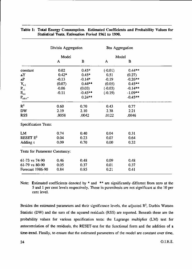
Table 1: Total Energy Consumption. Estimated Coefficients and Probability Values for Statistical Tests. Estimation Period 1961 to 1990.

Divisia Aggregation Btu Aggregation

Model Model A B A B

constant 0.02 0.45" (-0.01) 0.44"'

AP -0.13 -0.14* -0.19 -0.26"' A Y 0.42" 0.45' 0.5 1 (0.27)

y,- 1 (0.07) 0.44** (0.05) 0.45** pt-1 -0.06 (0.03) (-0.03) -0.14** Et4 -0.11 -0.45** (-0.19) -1.09** psa-1- 0.24** -0.45""

R2 DW RSS

0.60 0.70 0.43 0.77 2.19 2.10 2.38 2.2 1 .0058 -0042 -0122 .0046

Specification Tests:

LM 0.74 0.40 0.04 0.3 1 RESET E' 0.04 0.23 0.07 0.64 Adding t 0.09 0.70 0.00 0.32

Tests for Parameter Constancy:

61-73 VS 74-90 0.46 0.48 0.09 0.48 61-79 VS 80-90 0.05 0.37 0.01 0.37 Forecast 1986-90 0.84 0.85 0.21 0.41

Note: Estimated coefficients denoted by * and ** are significantly different from zero at the 5 and 1 per cent levels respectively. Those in parenthesis are not significant at the 10 per cent level.

Besides the estimated parameters and their significance levels, the adjusted R2, Durbin Watson

Statistic (DW) and the sum of the squared residuals (RSS) are reported. Beneath these are the

probability values for various specification tests: the Lagrange multiplier (LM) test for

autocorrelation of the residuals, the RESET-test for the functional form and the addition of a

time-trend. Finally, to ensure that the estimated parameters of the model are constant over time,

24 O.I.E.S.

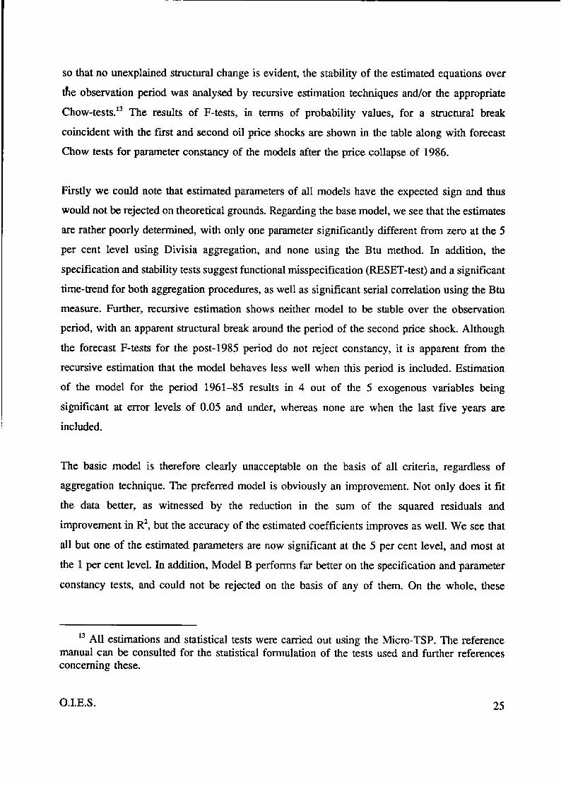
so that no unexplained structural change is evident, the stability of the estimated equations over

the observation period was analysed by recursive estimation techniques andlor the appropriate

Ch~w-tests.'~ The results of F-tests, in terms of probability values, for a structural break

coincident with the first and second oil price shocks are shown in the table along with forecast

Chow tests for parameter constancy of the models after the price collapse of 1986.

Firstly we could note that estimated parameters of alI models have the expected sign and thus

would not be rejected on theoretical grounds. Regarding the base model, we see that the estimates

are rather poorly determined, with only one parameter significantly different from zero at the 5

per cent Ievel using Divisia aggregation, and none using the Btu method. In addition, the

specification and stability tests suggest functional misspecification (RESET-test) and a significant

time-trend for both aggregation procedures, as well as significant serial correlation using the Btu measure. Further, recursive estimation shows neither model to be stable over the observation

period, with an apparent structural break around the period of the second price shock. Although

the forecast F-tests for the post-1985 period do not reject constancy, it is apparent from the

recursive estimation that the model behaves less well when this period is inchded. Estimation

of the model for the period 1961-85 results in 4 out of the 5 exogenous variables being

significant at error levels of 0.05 and under, whereas none are when the last five years are

included.

The basic model is therefore clearly unacceptable on the basis of all criteria, regardless of

aggregation technique. The preferred model is obviously an improvement. Not only does it fit

the data better, as witnessed by the reduction in the sum of the squared residuals and

improvement in R2, but the accuracy of the estimated coefficients improves as well. We see that

all but one of the estimated parameters are now significant at the 5 per cent level, and most at

the 1 per cent level. In addition, Model B perfoms far better on the specification and parameter

constancy tests, and could not be rejected on the basis of any of them. On the whole, these

l3 All estimations and statistical tests were carried out using the Micro-TSP. The reference manual can be consulted for the statistical formulation of the tests used and further references concerning these.

0.LE.S. 25

results leave little doubt about the superiority of Model B.

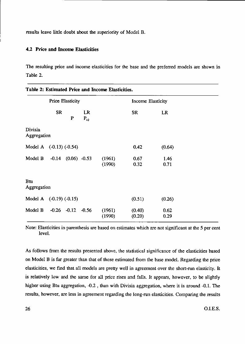
4.2 Price and Income Elasticities

The resulting price and income elasticities for the base and the preferred models are shown in

Table 2.

Table 2: Estimated Price and Income Elasticities.

Price Elasticity

SR LR p ps2

Divisia Aggregation

Model A (-0.13) (-0.54)

Model B -0.14 (0.06) -0.53 (1961) ( 1990)

Btu Aggregation

Model A (-0.19) (-0.15)

Model B -0.26 -0.12 -0.56 (1961) (1990)

Income Elasticity

SR LR

0.42

0.67 0.32

(0.64)

1.46 0.7 1

(0.5 1) (0.26)

(0.40) 0.62 (0.20) 0.29

Note: Elasticities in parenthesis are based on estimates which are not significant at the 5 per cent level.

As follows from the results presented above, the statistical significance of the elasticities based

on Model B is far greater than that of those estimated from the base model. Regarding the price

elasticities, we find that all models are pretty well in agreement over the short-run elasticity. It

is relatively low and the same for all price rises and falls. It appears, however, to be dightly

higher using Btu aggregation, -0.2 , than with Divisia aggregation, where it is around -0.1. The

results, however, are less in agreement regarding the long-run elasticities. Comparing the results

26 O.I.E.S.

of the basic model for the two aggregation methods, we see that the long-run price elasticity is

far greater using Divisia aggregation, although neither is statistically significant. There is more

agreement with Model B. In both cases, long-run demand has responded substantially to the

1979-81 price increases, with an elasticity of around -0.5, but has been more-or-less unresponsive

to other price changes, including the price collapse. We have, however, slightly different results

concerning reversibility. With Divisia aggregation, demand appears to be totally unresponsive to

all but the price increases of 1979-8 1, so that the reduction in demand associated with these price

rises is totally irreversibIe. Using Btu aggregation, on the other hand, indicates a statistically

significant, albeit relatively low general elasticity of -0.1. The demand reduction generated by

the second price shock is in this case partiaIly reversible, so that about one-quarter of it will be

regained as prices return to pre-1979 levels. One can, however, question the Btu estimates since

they are based on a price index which not only reflects actual price changes, but also an

increasing share of dearer fuels.

Comparing the long and short-run elasticities for Model B indicates a short-run over-shooting of

demand to general price changes. There appears to be an immediate over-reaction, which is

generally short lived, as consumption returns more-or-less to its initial level over time. The

interpretation of this phenomenon would be different for price rises and price falls. For price

increases, a partid explanation could lie in the substitution between energy forms. Since the

prices of the individual forms of energy included in the aggregate need not change in proportion

to the aggregate price, a rise in aggregate prices will generally be associated with a change in

relative prices. Given minimal possibilities for short-run substitution, the initial response to a

price increase can only be a reduction in total consumption. Over time, however, the substitution

induced by the change in relative prices will increase the demand for energy forms which have

become reIatively cheaper, thereby increasing total consumption, so that at least part of the initial

effect will be reversed. This argument would not be tenable for a price decrease, however. In this

case, the only possible explanation could be that lower prices initially stimulate demand above

its optimal level, but over time demand decIines again as consumers divert their increase in

purchasing power to other goods.

We now turn OUT attention to the income elasticities. For the declining elasticity models two

0.LE.S. 27

values for each of the short- and long-run elasticities are given: for 1961 and for 1990, the first

and last years of the data sample. For both aggregation methods, we find that the estimates for

the constant elasticity model lie within the interval indicated for that with a declining elasticity.

In all instances, the elasticity is greater in the long run than in the short run. It is not obvious that

this need be the case, but it is somewhat more intuitive than the reverse.

Comparing the results using Divisia and Btu aggregation, we find that the short-run elasticities

are rather similar, but that substantial differences occur in the long run. As we had surmised on

the basis of the development of the energy-GDP ratio, the long-run elasticity using Btu

aggregation is well below unity for the entire period. Further, the Divisia index yields a far

higher value. As discussed previously, this is exactly as we would expect. The Divisia measure

of energy consumption reflects qualitative changes in energy demand: in the sixties and early

seventies from coal to oil and gas and in the later seventies and the eighties from heavier oil

products to electricity and motor fuels. Rising income has led not only to a greater energy

demand, measured in physical units, but also to a shift in the composition of demand over time

towards more expensive forms of energy. The magnitude of this ‘quality’ change can be seen by

comparing the elasticities based on the two aggregation techniques. The impact of a rise in

income on physical energy use is given by the Btu elasticity. For our preferred model, B, the

long-run impact of a 1 per cent increase in GDP is about 0.3 per cent for 1990. This effect along

with the qualitative effect is measured by the Divisia elasticity, which indicates a 0.7 per cent

increase, for the comparable model and year. From this we see that the qualitative effect of

income on energy demand is at least as large as the physical.

Another major difference between the two aggregation methods concerns the speed of adjustment.

With Btu aggregation the mean lag is less than one year for both price and income, while it is

3.5 for price and 2 years for income with the Divisia measure. The near instantaneous adjustment

of the Btu measure suggests that the Divisia aggregation procedure is more able to capture the

dynamics of adjustment. The slower adjustment of the Divisia measure to income changes is

easily explained: a rise in GDP rapidly induces an increase in physical energy consumption @tu);

over time, it also stimulates a substitution towards dearer energy sources. The differences in

adjustment to price changes are more difficult to expIain since both price and quantity measures

28 O.I.E.S.

differ using the two aggregation techniques.

4.3 Tests Concerning the Specification of the Income Elasticity

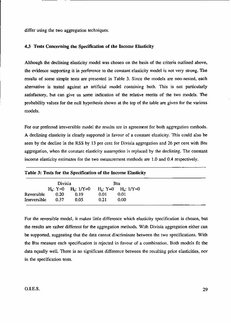
Although the declining elasticity model was chosen on the basis of the criteria outlined above,

the evidence supporting it in preference to the constant eIasticity model is not very strong. The

results of some simple tests ace presented in Table 3. Since the models are non-nested, each

alternative is tested against an artificial model containing both. This is not particularly

satisfactory, but can give us some indication of the relative merits of the two models. The

probability values for the null hypothesis shown at the top of the table are given for the various

models.

For our preferred irreversible model the results are in agreement for both aggregation methods.

A declining elasticity is clearly supported in favour of a constant elasticity. This could also be

seen by the decline in the RSS by 13 per cent for Divisia aggregation and 26 per cent with Btu

aggregation, when the constant elasticity assumption is replaced by the declining. The constant

income elasticity estimates for the two measurement methods are 1.0 and 0.4 respectively.

Table 3: Tests for the Specification of the Income EIasticity

Divisia Btu &:Y=o &: 1/Y=o &:Y=O H,: 1/Y=o

Reversible 0.20 0.19 0.01 0.01 Irreversible 0.37 0.05 0.21 0.00

For the reversible model, i t makes little difference which elasticity specification is chosen, but

the results are rather different for the aggregation methods. With Divisia aggregation either can

be supported, suggesting that the data cannot discriminate between the two specifications. With

the Btu measure each specification is rejected in favour of a combination. Both models fit the

data equally well. There is no significant difference between the resulting price elasticities, nor in the specification tests.

O.I.E.S. 29

4.4 Tests for Price Reversibility

As outlined in Section 3.2, three different hypotheses regarding the impact of prices on demand

were posited as alternatives to the base model. Our first step in choosing the final specification

was to see whether any of the alternative specifications provide a better description of the data

than the reversible models, by testing the long-run significance of P+, P, and P,, individually.

The results are shown in Table 4 for both the constant (C) and declining (D) elasticity models,

using both Btu and Divisia aggregation.

The numbers shown in the first three rows of Table 4 refer to the probability values for the null

hypothesis of equal price effects against the alternative specification shown in the left hand

column. They are based on F-tests for the null hypothesis, H,, shown in the second column, Low

probability values lead to the rejection of H,,, and thus the base rnudel, in favour of the

specification tested. The last three rows test specific hypotheses concerning the effects of the two

price rises and the price collapse, given the price shock model.

Table 4: Tests for Price Specifications for Constant (C) and Declining (D) Elasticity Models. Probability Values for F- or t-tests of H,.

Divisia Btu C D C D

Jagged-Ratchet P+=O 0.07 0.06 0.01 0.01

Price Shock P, =P,,=P,,=O 0.02 0.01 0.00 0.00

ps,=o 0.01 0.0 1 0.00 0.00

Ratchet P,=O 0.13 0.13 0.04 0.01

P S l a 0.08 0.19 0.15 0.99

ps,=o 0.38 0.37 0.26 0.22

From these results we see that the base model is rejected in favour of at least one of the

alternative specifications in all cases. Using Divisia aggregation, we find that only the price shock

model is supported with any confidence, whereas using Btu aggregation the base model is

30 O.I.E.S.

rejected in favour of all three alternatives. Further testing of the price shock model, reported in

the rows below, indicates that only the elasticity associated with the second price shock is

significantly different from that for other price changes. Given that Fs,= 0 cannot be rejected, the

effects on demand of the price rises of 1979-81 appears to be irreversible. Thus reversibility is

rejected with the price shock model regardless of aggregation method or the specification of the

income elas ticity.

0.LE.S. 31

32 0.LE.S.

5 CONCLUSIONS

We have Seen that the traditional energy demand model provides a rather unsatisfactory

description of energy demand over the past thee decades. The resuIting estimates are surrounded

by a high degree of uncertainty, and the model performs poorly on specification and stability

tests. We have also seen that r e k i n g some of the assumptions inherent in this model vastly

improves the resulting estimates by all these criteria. Most critical is the assumption that demand

responds with equal elasticity to all price changes. The empirical evidence strongly suggests that

this has not been the case. Demand appears to have reacted substantially to the price increases

of 1979-81, with m elasticity of -0.5, but has been much less sensitive to all other price changes,

including the price collapse of 1986. Excluding the price increases of the later seventies, we find

an elasticity on the order of -0.1. Demand is thus not perfectly reversible to price changes as is

traditionally assumed. The reaction to the price increases of the late seventies, as measured by

the price elasticity, was five times greater than the response to the price collapse. The era of high

oil prices has undeniably had - and will continue to have - a persistent dampening effect on

demand, which will not be totally reversed under any feasible price scenario. This conclusion is supported regardless of the specification of the income elasticity and the method used to

aggregate energy quantities and prices.

The assumption of an unchanging long-run energy demand relationship is clearly inconsistent

with the empirical evidence, and is therefore unsuitable for explaining energy demand over the

past three decades, or for the future. The persistence of lower demand levels despite the reversal

of prices can only be explained in krms of a hysteresis or structural break in the demand

relationship, triggered by the era of high energy prices, which has shifted the demand curve

downwards. The underlying mechanism is surely complex, but there are a number of likely

explanations. Firstly, high energy prices have induced the development of more energy-efficient

technologies, which were non-existent in the early seventies. Given the irreversibility of technical

progress, and the fact that some of these technologies are economically optimal even at lower

energy prices, many of these will continue to be employed in favour of those used in the early

seventies, thus permanently reducing energy requirements. Although investments in energy

efficiency which are not economically justifiable at lower price levels will not continue to be

0.LE.S. 33

made, the sunk-cost nature of these and longevity of capital involved mean that those made in

the past will remain in place, thus affecting demand for some time to come, even if they are

theoretically ‘reversible’. Another explanation lies in smctural change. Although the decline of

manufacturing, and particularly heavy industry, may be the result of more wide-ranging economic

forces, high energy prices may have accelerated this processs, by worsening the competitive

position of already ailing industries. A return to Iower energy prices will hardly reverse this

trend.

Of course one could argue that improvements in energy efficiency have reduced the cost of

energy services even more than that implied by the decline in the price of energy. Consumers

will thus increase their demand for these services all the more. Although this is undeniable to

some degree, the evidence suggests that this additional demand falls short of the savings realized.

AIthough the estimated price-elasticity may appear ‘low’, we must keep in mind that it refers to

total energy demand. We would expect total demand to be less price responsive than the demand

for each individual fuel in all but two circumstances: if there were no substitution possibilities

amongst fuels, or if the prices of all fuels changed in the same proportion. Clearly neither of

these conditions hold. The relative ‘inelasticity’ of total demand with respect to the aggregate

price is thus not inconsistent with a substantial substitution amongst energy forms, and high

individual price elasticities.

Relaxation of the constant income elasticity assumption does not affect the estimates as

dramatically, dthough there is some empirical support for a decfining elasticity over the

observation period. The income elasticity estimates are, however, highly sensitive to the definition

of the energy aggregate. With the Divisia measure, there is a decline from above unity in the

1960s to around 0.7 in 1990. When energy is measured in physical terms, it is below unity over

the entire period, from around 0.6 in the sixties to 0.3 in 1990. The difference between these two

elasticities is explained primarily by two factors. The Divisia elasticity measure partially reflects

the qualitative change in energy consumption towards more costIy energy products. The physical

energy income elasticity, being measured on a heat-supplied, rather than a useful energy basis,

partially reflects the substitution towards more efficient fuels. A more accurate measure of the

34 0.LE.S.

effect of income would be in terns of useful energy, since consumer demand for energy arises

from the demand for energy services, rather than for energy per se. Although we would expect

the Divisia measure to give a closer approximation to this, estimation based on useful energy and

its price would be the most appropriate.

The evidence suggests that the price increases of the seventies and eighties have led to a

reduction in long-run demand of 14 per cent, most of which will not be recaptured as prices fall.

High energy prices have also clearly contributed to the falling energy-GDP ratio observed since

1973, but more than half of the decline must be explained by non-price related factors. Given the

simplicity of our model all these factors - be they structural change, general (non-price induced)

improvements in energy efficiency, saturation levels for certain energy uses - are summarized

in the income variable. An income elasticity of below unity as evidenced by our results reduced

the energy-GDP ratio over this period at least as substantially as did energy prices. Structural

change appears to have been a predominant factor: reducing the energy intensity of GDP as

production shifted from heavy industry to high-tech products and as the service sector has gained

in importance over manufacturing production. For the pre-1973 period, the 19 per cent decline

in the physical energy-GDP ratio is primarily explained by the same phenomena. During this

earlier period, howeve?, it Seems that the primary factor was general improvements in energy

efficiency in new capital, spurred by rapid economic growth and investment, while structural

change played a minor r01e.l~ Over the period as a whole, higher incomes have made energy

use for residential purposes more of an inferior good as saturation levels are being approached.

The positive effects on energy consumption of rising income have largely been of a qualitative

nature, as the composition of demand has shifted toward higher quality products, such as electricity and motor fuels.

It is likely that many of the processes at work during the seventies and eighties described above

will continue into the nineties, so that we can expect a further decline in the energy-GDP ratio,

regardless of price development. Although energy consumption will continue to grow, the rapid

l4 Jenne and Cattell (1983).

0.LE.S. 35

growth rates and the high energy-GDP ratios prevailing in the sixties and the seventies are an

event of the past.

Our resdts have important implications both for forecasting future demand and for accessing

the viability of price-related policy measures aimed at curtailing the growth of energy demand.

As reversible models tend to ‘average out’ the price elasticity, projections of future demand based

on such elasticities will be highly dependent on the period of estimation. Particularly, elasticities

based on the period ending in the mid-eighties (-0.3 to -0.4) wil1 tend to overestimate the effect

of falling prices, while estimates based on post-85 data (-0.1 to -0.2) will tend to underestimate

the impact of substantial price rises. The irreversible model, on the other hand, indicates that

demand is not particularly sensitive to minor price changes, or even to a considerable price fall

following a period of historically high prices (a long-run elasticity of -0.1). However,

considerable and sustained price rises, such as those experienced in 1979 to 1981, have reduced

demand significantly (an elasticity of -0.5). From this it appears that prices can be a viable

instrument in reducing energy demand, but that substantial price rises would be necessary in

order to achieve a significant effect.

We must, however, be careful in extrapolating from the past. As our results confirm, long-run

energy demand is determined not only by prices, but also by the evolution of prices over time.

The price increases of the 1970s were unprecedented historically, and followed a long period of

low energy prices. The possibilities of reducing energy use were substantial. Given that much of

the reduction in demand triggered by the price shocks remains, in the form of improved

efficiency, induced structural change or behavioural modification, it couid be argued that further

reductions in consumption may not be as easily achieved. Adjustment to high energy prices has

reduced the flexibility of energy demand, so that much larger price increases might be required

to induce a similar reduction today. Unfortunately this must all remain specuIation; only in the

event will the answer be known. Until then, we have only the experience of the past to guide us.

It seems clear that abandoning the reversibility assumption gives us a better basis for

understanding the past and thereby for making projections into the future.

36 O.I.E.S.

REFERENCES

Berndt, E. R. (1978), ‘Aggregate energy, efficiency and productivity’, Annual Review of Energy, vol. 3, pp. 225-73.

Brown, S. P. A. and K. R. Phillips (1990), ‘US oil demand and conservation’, Contemporary P d i ~ y ISSUS, vol. 9, January, pp. 67-72.

Bye, T. (1987) ‘Non-symmetric responses in energy demand?’, in D. 0. Wood (ed.), The Changing World Energy Economy, Proceedings of the Eighth Annual North American Conference November 1986, International Association of Energy Economists, May, pp. 354-8.

Dargay, J. M. (1990), Have Low Oil Prices Reversed the Decline in Energy Demand? A Case Study for ?he UK, Oxford Institute for Energy Studies, Working Paper EE9.

Dargay, J. M. (19911, The Irreversible Demand E$ects of High Oil Prices: Motor Fuels in France, Germany and the UK, Oxford Institute for Energy Studies, Working Paper EE 13.

Department of Energy (19891, ‘The demand for energy’, in D. Helm, J. Kay and D. Thompson (eds), The Marketfor Energy, Clarendon Press, Oxford, pp. 77-91.

Gately, D. and P. Rappoport, (1988), ‘The adjustment of US oil demand to the price increases of the 1970s’, The Energy Journal, vol. 9, no. 2, pp. 93-107.

Gately, D. (19911, Impetfieet Price-Reversibiliv of US Gasoline Demand: Asymmetric Responses to Price incremes and Declines, C. V. Starr Center for Applied Economics, Economic Research Report pp. 91-55, New York University.

Houck, J. P. (1977), ‘An approach to specifying and estimating nonreversible functions’, American Journal of Agricultural Economics, vol. 59, pp. 570-72.

Humphreys, W.S. and J.Stanis1aw (1979) ‘Economic growth and energy consumption in the UK, 1700 to 1975’, Energy Policy, vol. 7, no.1. pp. 2942.

Hunt, L, and N. Manning (1989), ‘Energy price- and income elasticities of demand: some evidence for the UK using the cointegration procedure”, Scottish Journal of Political Economics, vol. 36, no. 2, pp. 183-193.

Jenne, C.A and R.K. Cattell (1983) ‘Structural change and energy efficiency in industry’ Energy Economics vol. 5, no. 2, pp. 114-23.

O.I.E.S. 37

Kourvaritakis, N. (1987), The IEA Experience in Assessing the Impact of Lower Energy Prices, Energy Demand Analysis Symposium, Paris.

Kouris, G. (1980), ‘Energy modelling: the economist’s approach’, in W. Hafele (ed.), Modelling of Large-Scale Energy Systems, Proceedings of the IIASMFAC Symposium.

Kouris, G. (1983), ‘Energy demand elasticities in industrialized countries: a survey’, The Energy Journal, vol. 4, no. 3, pp. 73-94.

Mittelstadt, A. (1983), Use of Demand Elasticities in Estimating Energy Demand, OECD Working Paper Series, ESD No. 1.

Nguyen, H. V. (1987), ‘Energy elasticities under Divisia and Btu aggregation’, Energy Economics, vol. 9, no. 4, pp. 210-14.

Traill, B., D. Colman and T. Young (1978), ‘Estimating irreversible supply functions’, American Journal of Agricultural Economics, vol. 60, August, pp. 528-3 1.

Shealy, M. (1990), ‘Oil demand asymmetry in the OECD’, in Proceedings of the International Association of Energy Economists, Twelfth Annual North American Conference, Ottawa, Canada.

Sweeney, J. L. and D. A. Fenichel (1987), ‘Price asymmetries in the demand for energy’, in P. Stevens (ed.), Energy Demand: Prospects and Trends, Macmillan, London.

Watkins, G. C. and L. Waverman (1987), ‘Demand elasticities: the saviour as well as the scourge of OPEC’, in D. 0. Wood (ed.), op cit, pp. 223-7.

Welsch, H. (1989), ‘The reliability of aggregate energy demand functions: an application of statistical specification error tests’, Energy Economics, vol. 1 1, no. 4, pp. 285-92.

Wirl, F. (1988) ‘The asymmetrical energy demand pattern: some theoretical explanations’, OPEC Review, vol. XII, no. 4, pp. 353-67.

Wolffm, R. (1971), ‘Positivistic measures of aggregate supply elasticities: some new approaches - some critical notes’, American Journal of Agricultural Economics, vol. 53, pp. 356-9.

O.I.E.S. 38

OXFORD INSTITUTE FOR ENERGY STUDIES 57 WOODSTOCK ROAD, OXFORD OX2 6FA ENGLAND

TELEPHONE (01865) 311377 FAX (01365) 310527

E-mail: publications@oxfordenergy.org http:/lwww.oxfordenergy.org