GMS Tutorials MODFLOW v. 10gmstutorials-10.4.aquaveo.com/MODFLOW-ConceptualModel...If GMS is already...

GMS Tutorials MODFLOW – Conceptual Model Approach 3

of 13 © Aquaveo 2018

00

GMS 10.4 Tutorial

MODFLOW – Conceptual Model Approach 3 Build a multi-layer MODFLOW model using advanced conceptual model techniques

Objectives The conceptual model approach involves using the GIS tools in the Map module to develop a conceptual

model of the site being modeled. The location of sources/sinks, layer parameters such as hydraulic

conductivity, model boundaries, and all other data necessary for the simulation can be defined at the

conceptual model level without a grid.

Prerequisite Tutorials MODFLOW – Conceptual

Model Approach 1 and 2

MODFLOW – Interpolating

Layer Data

Required Components Grid Module

Geostatistics

Map Module

MODFLOW

Time 35–50 minutes

v. 10.4



1 Introduction ......................................................................................................................... 2 1.1 Getting Started ............................................................................................................. 3

2 Importing the Project ......................................................................................................... 4 3 Saving the Project ............................................................................................................... 4 4 Creating the Grid ................................................................................................................ 4 5 Initializing the MODFLOW Data ...................................................................................... 5 6 Defining the Active/Inactive Zones .................................................................................... 5 7 Redefining the Hydraulic Conductivity ............................................................................ 6

7.1 Creating the Layer 2 Coverage ..................................................................................... 7 8 Interpolating Layer Elevations .......................................................................................... 7

8.1 Interpolating the Surface Elevations ............................................................................ 7 8.2 Interpolating the Layer Elevations ............................................................................... 8 8.3 Viewing the Model Cross Sections .............................................................................. 8 8.4 Fixing the Elevation Arrays ......................................................................................... 9

9 Converting the Conceptual Model ................................................................................... 10 10 Checking and Saving the Simulation ............................................................................... 10 11 Running MODFLOW ....................................................................................................... 11 12 Viewing the Water Table in Side View ............................................................................ 11 13 Fixing the Well .................................................................................................................. 12 14 Conclusion.......................................................................................................................... 13

1 Introduction

This tutorial builds on the “MODFLOW – Conceptual Model Approach 1” and

“MODFLOW – Conceptual Model Approach 2” tutorials. In those tutorials, a one-layer

model using the conceptual model approach was built. The top and bottom elevations

were all the same, meaning the model was completely flat.

This tutorial takes that model and makes it more complex and realistic. It is modified to

have two layers and varying top and bottom elevations that match the terrain and

geology. One of the wells will be assigned to layer 2.

The problem solved in this tutorial is a site in East Texas as illustrated in Figure 1. This

tutorial evaluates the suitability of a proposed landfill site with respect to potential

groundwater contamination. The results of this simulation are used as the flow field for a

particle tracking and a transport simulation in the MODPATH and MT3DMS tutorials.

The simulation models the groundwater flow in the valley sediments bounded by the hills

to the north and the two converging rivers to the south. A typical north-south cross

section through the site is shown in Figure 1b. The site is underlain by limestone bedrock

which outcrops to the hills at the north end of the site. There are two primary sediment

layers: an upper layer modeled as an unconfined, and the lower layer modeled as

confined.

The boundary to the north is a no-flow boundary, and the remaining boundary is a

specified head boundary corresponding to the average stage of the rivers. The system is

primarily recharged through rainfall. Creek beds in the area are usually dry but

occasionally flow due to influx from the groundwater. The tutorial model represents these

creek beds using drains. Two production wells in the area are included in the model.

Although the site modeled in this tutorial is an actual site, the landfill and the

hydrogeologic conditions at the site have been fabricated. The stresses and boundary

conditions used in the simulation were selected to provide a simple—yet broad—

sampling of the options available for defining a conceptual model.



River

Limestone Bedrock

River

(b)

Well #1

Well #2

Proposed

Landfill

Site

RiverCreek beds

Limestone Outcropping

North

(a)

Upper Sediments

Lower Sediments

Figure 1 Site to be modeled in this tutorial. (a) Plan view of site. (b) Typical north-south cross section through site

This tutorial will discuss and demonstrate:

Creating a two layer grid from the conceptual model.

Interpolating scatter points to MODFLOW layer data.

Mapping the conceptual model to MODFLOW.

Adjusting the well depth.

Checking the simulation and running MODFLOW.

Viewing the results.

1.1 Getting Started

Do the following to get started:

1. If necessary, launch GMS.

2. If GMS is already running, select File | New to ensure that the program settings

are restored to their default state.



2 Importing the Project

The first step is to import the East Texas project. This opens the MODFLOW model, the

solution, and all other files associated with the model.

To import the project, do as follows:

1. Click Open to bring up the Open dialog.

2. Select “Project Files (*.gpr)” from the Files of type drop-down.

3. Browse to the modfmap3 directory and select “start.gpr”.

4. Click Open to import the project and close the Open dialog.

The Main Graphics Window will appear as in Figure 2.

Figure 2 After importing the project

3 Saving the Project

Before making any changes, save the project under a new name.

1. Select File | Save As… to bring up the Save As dialog.

2. Select “Project Files (*.gpr)” from the Save as type drop-down.

3. Enter “EastTexas3.gpr” as the File name.

4. Click Save to save the file under the new name and close the Save As dialog.

Be sure to periodically Save throughout the tutorial.

4 Creating the Grid

Start with creating a new two layer grid.

1. Select Feature Objects | Map → 3D Grid to get the first of two warning

messages.

2. Click OK at the warning dialog to delete the existing grid.



3. Click OK to delete the existing MODFLOW simulation and to open the Create

Finite Difference Grid dialog.

Notice that the grid is dimensioned using the data from the grid frame. If a grid frame

does not exist, the grid is defaulted to surround the model with approximately 5% overlap

on the sides.

4. Under the X-Dimension and Y-Dimension sections, select Cell Size and enter

“20.0”.

5. In the Z-Dimension section, select Number cells and enter “2” in the field to the

right.

6. Click OK to close the Create Finite Difference Grid dialog.

The new grid will appear in the Graphics Window (Figure 3).

Figure 3 The two layer grid

5 Initializing the MODFLOW Data

Now that the grid is constructed, the next step is to convert the conceptual model to a

grid-based numerical model. Before doing this, the MODFLOW data must first be

initialized:

1. Right-click on the “ grid” in the Project Explorer and select New

MODFLOW… to bring up the MODFLOW Global/Basic Package dialog.

2. Click OK to accept the defaults and close the MODFLOW Global/Basic Package

dialog.

6 Defining the Active/Inactive Zones

Now that the grid has been created and MODFLOW has been initialized, the next step is

to define the active and inactive zones of the model. This is accomplished automatically

using the information in the map coverage. However, the existing map coverages are set

up for a one layer grid. They will need to be modified to apply to both layers of the grid.

1. Select the “ Rivers” coverage to make it active.



2. Right-click on “ Rivers” and select Coverage Setup to open the Coverage

Setup dialog.

3. Turn on Layer Range under the Source/Sinks/BCs section.

4. Click OK to close the Coverage Setup dialog.

Turning on the Layer Range option overwrites the Default Layer Range and allows each

feature object in the coverage to be assigned its own layer range. New objects created on

the coverage after this option is active will automatically use the full layer range. Existing

objects will need to be modified.

5. Using the Select Polygons tool, select the polygon.

6. Click Properties to bring up the Attribute Table dialog.

7. Scroll to the far right in the table and confirm that the layer assignment for the

From layer is “1” and the To layer is “2”.

8. Click OK to close the Attribute Table dialog.

Other coverages and feature objects do not need to be adjusted at this time.

9. Click anywhere outside the polygon to unselect it.

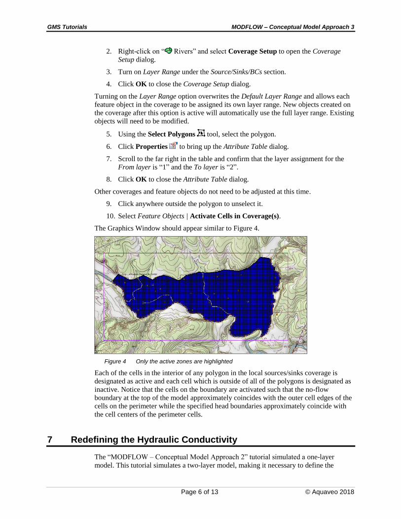
10. Select Feature Objects | Activate Cells in Coverage(s).

The Graphics Window should appear similar to Figure 4.

Figure 4 Only the active zones are highlighted

Each of the cells in the interior of any polygon in the local sources/sinks coverage is

designated as active and each cell which is outside of all of the polygons is designated as

inactive. Notice that the cells on the boundary are activated such that the no-flow

boundary at the top of the model approximately coincides with the outer cell edges of the

cells on the perimeter while the specified head boundaries approximately coincide with

the cell centers of the perimeter cells.

7 Redefining the Hydraulic Conductivity

The “MODFLOW – Conceptual Model Approach 2” tutorial simulated a one-layer

model. This tutorial simulates a two-layer model, making it necessary to define the



hydraulic conductivity for the second layer. Similar to in the previous tutorial, the second

layer uses constant values.

7.1 Creating the Layer 2 Coverage

To facilitate the two-layer model simulation, create the “Aquifer Layer 2” coverage by

copying the “Aquifer Layer 1” coverage.

1. Right-click on “ Aquifer Layer 1” and select Duplicate… to create a new “

Copy of Aquifer Layer 1” coverage.

2. Right-click on “ Copy of Aquifer Layer 1” and select Coverage Setup… to

bring up the Coverage Setup dialog.

3. Enter “Aquifer Layer 2” as the Coverage name.

4. Below the three columns, set the Default layer range to go from “2” to “2”.


8 Interpolating Layer Elevations

Now it is necessary to define the layer elevations. Since this tutorial uses the LPF

package, top and bottom elevations are defined for each layer regardless of the layer type.

For a two layer model, it is necessary to define a layer elevation array for the top of layer

1 (the ground surface), the bottom of layer 1, and the bottom of layer 2. It is assumed that

the top of layer 2 is equal to the bottom of layer 1.

One way to define layer elevations is to import a set of scatter points defining the

elevations and interpolate the elevations directly to the layer arrays. This can be done

with scatter points as well as rasters. In this case, use a raster for the top of the grid and

scatter points for the elevations of the bottom of layer 1 and the bottom of layer 2.

Layer interpolation is covered in depth in the “MODFLOW – Interpolating Layer Data”

tutorial.

8.1 Interpolating the Surface Elevations

To interpolate the ground surface elevations to the MODFLOW grid, do the following:

1. In the Project Explorer, expand the “ GIS Layers” folder.

2. Right-click on the “ elev_10.tif” raster and select Interpolate To |

MODFLOW Layers… to bring up the Interpolate to MODFLOW Layers

dialog.

This dialog tells GMS which datasets to interpolate to which MODFLOW arrays. The

dialog is explained fully in the “MODFLOW – Interpolating Layer Data” tutorial.

3. Select “elev_10.tif” in the Rasters section and “Top Elevations Layer 1” in the

MODFLOW data section.

4. Click Map to add them to the Dataset → MODFLOW data section.



5. Click OK to perform the interpolations and close the Interpolate to MODFLOW

Layers dialog.

8.2 Interpolating the Layer Elevations

To interpolate the layer elevations for the bottom of layers 1 and 2, do the following:

1. In the Project Explorer, expand the “ 2D Scatter Data” folder.

2. Right-click on the “ elevs” scatter set and select Interpolate To | MODFLOW

Layers to bring up the Interpolate to MODFLOW Layers dialog.

Notice that GMS automatically mapped the Bottom Elevations Layer 1 and Bottom

Elevations Layer 2 arrays to the appropriate datasets based on the dataset name. No

additional mappings need to be performed here.

3. Click OK to perform the interpolations and close the Interpolate to MODFLOW

Layers dialog.

Now that the interpolation is finished, hide the scatter point sets, GIS layers, and the grid

frame.

4. Turn off the “ Grid Frame”, the “ GIS Layers” folder, and the “ 2D

Scatter Data” folder.

8.3 Viewing the Model Cross Sections

To check the interpolation, view a cross section.

1. Select the “ 3D Grid Data” folder in the Project Explorer.

2. Using the Select Cell tool, select a cell somewhere near the center of the

model.

3. Switch to Side View .

4. Use the arrow buttons in the Tool Palette to view different columns in the grid.

Note that on the right side of the cross section, the bottom layer pinches out and the

bottom elevations are greater than the top elevations (Figure 5). This must be fixed before

running the model.

Figure 5 Cross section before elevations are corrected



8.4 Fixing the Elevation Arrays

GMS provides a convenient set of tools for fixing layer array problems. These tools are

located in the Model Checker and are explained fully in the “MODFLOW – Interpolating

Layer Data” tutorial.

1. Select MODFLOW | Check Simulation… to bring up the Model Checker dialog.

2. Click Run Check to check the model for errors.

Notice that many errors were found for layer 2. There are several ways to fix these errors.

This tutorial will use the Truncate to bedrock option. This option makes all cells below

the bottom layer inactive.

3. Click Fix Layer Errors… to bring up the Fix Layer Errors dialog.

4. In the Correction method section, select Truncate to bedrock and click Fix

Affected Layers.

5. Click OK to exit the Fix Layer Errors dialog.

6. Click Run Check to check the model for errors.

Notice that all the errors have been fixed. The various warnings are acceptable for the

purposes of this tutorial and can be ignored.

7. Click Done to exit the Model Checker dialog.

Another way to view the layer corrections is in plan view.

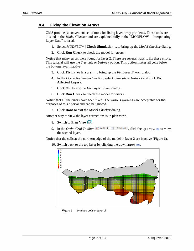
8. Switch to Plan View .

9. In the Ortho Grid Toolbar , click the up arrow to view

the second layer.

Notice that the cells at the northern edge of the model in layer 2 are inactive (Figure 6).

10. Switch back to the top layer by clicking the down arrow .

Figure 6 Inactive cells in layer 2



9 Converting the Conceptual Model

It is now possible to convert the conceptual model from the feature object-based

definition to a grid-based MODFLOW numerical model.

1. Right-click on the “ East Texas” conceptual model and select Map To |

MODFLOW / MODPATH to bring up the Map → Model dialog.

2. Select All applicable coverages and click OK to close the Map → Model dialog.

Notice that the cells underlying the drains, wells, and specified head boundaries were all

identified and assigned the appropriate sources/sinks (Figure 7). The heads and elevations

of the cells were determined by linearly interpolating along the specified head and drain

arcs. The conductances of the drain cells were determined by computing the length of the

drain arc overlapped by each cell and multiplying that length by the conductance value

assigned to the arc. In addition, the recharge and hydraulic conductivity values were

assigned to the appropriate cells.

Figure 7 The model after conversion

10 Checking and Saving the Simulation

At this point, the MODFLOW data has been completely defined, and it is possible to run

the simulation. First run the Model Checker again to see if GMS can identify any

mistakes that may have been made.

1. Select the “ 3D Grid Data” folder in the Project Explorer to switch to the 3D

Grid module.

2. Select MODFLOW | Check Simulation… to bring up the Model Checker dialog.

3. Click Run Check. There should be no errors.

4. Click Done to exit the Model Checker dialog.

5. Save the project.

Saving the project not only saves the MODFLOW files but it saves all data associated

with the project including the feature objects and scatter points.



11 Running MODFLOW

It is now possible to run MODFLOW.

1. Select MODFLOW | Run MODFLOW to bring up the MODFLOW model

wrapper dialog. The process should be completed quickly.

2. When the solution is completed, turn on Read solution on exit and Turn on

contours (if not on already) and click Close to exit the MODFLOW model

wrapper dialog.

The Graphics Window should appear similar to Figure 8. To view the contours for the

second layer, do as follows:

3. Click the up arrow in the Ortho Grid Toolbar.

4. After viewing the contours, return to the top layer by clicking the down arrow .

Figure 8 Contours of layer 1 after the model run

Notice the flooded cells (indicated by the small blue symbols) along parts of the river

boundaries. These areas are flooded at generally less than one foot and show how the

water table is very near the surface in those areas.

12 Viewing the Water Table in Side View

An interesting way to view a solution is in side view.

1. Using the Select Cell tool, select a cell somewhere near the well on the right

side of the model.


Notice that the computed head values are used to plot a water table profile.

3. Use the arrow buttons in the Mini-grid Toolbar to move back and forth

through the grid.

Notice the well does not extend into the second layer as shown in Figure 9. This will need

to be fixed.



Figure 9 Side view of the model

13 Fixing the Well

The well on the right side currently only extends to the bottom of the first layer. To fix

this, do the following:

1. Switch to Plan View .

2. Select “ Wells” to make it active.

3. Right-click on “ Wells” and select Coverage Setup to open the Coverage

Setup dialog.

4. Turn on Layer Range under the Source/Sinks/BCs section.


6. Using the Select Points/Nodes tool, double-click on the well on the right side

to bring up the Attribute Table dialog.

7. Scroll to the far right in the table and confirm that the layer assignment for the

From layer is “1” and the To layer is “2”.

8. Click OK to close the Attribute Table dialog.

Modifying the number of layers included in a well also changes the well flow to be

partitioned between the layers based on the relative transmissivity of each layer.

Next, add the changes to the simulation.

9. Right-click on the “ East Texas” conceptual model and select Map To |

MODFLOW / MODPATH to bring up the Map → Model dialog.

10. Select All applicable coverages and click OK to close the Map → Model dialog.

With the changes to the well applied to the simulation, run MODFLOW again.

11. Click Save .

12. Select MODFLOW | Run MODFLOW to bring up the MODFLOW model

wrapper dialog. The process should be completed quickly.

13. When the solution is completed, turn on Read solution on exit and Turn on

contours (if not on already) and click Close to exit the MODFLOW model

wrapper dialog.

The results of these changes can be reviewed by doing the following:



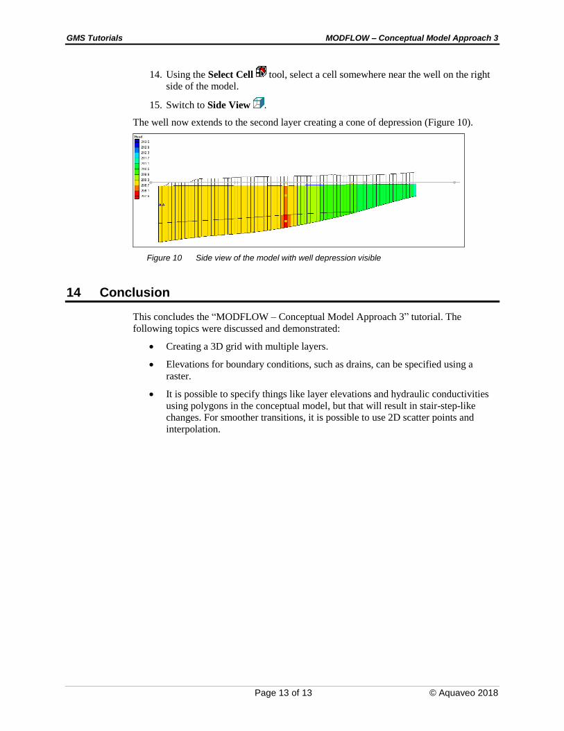
14. Using the Select Cell tool, select a cell somewhere near the well on the right

side of the model.


The well now extends to the second layer creating a cone of depression (Figure 10).

Figure 10 Side view of the model with well depression visible

14 Conclusion

This concludes the “MODFLOW – Conceptual Model Approach 3” tutorial. The

following topics were discussed and demonstrated:

Creating a 3D grid with multiple layers.

Elevations for boundary conditions, such as drains, can be specified using a

raster.

It is possible to specify things like layer elevations and hydraulic conductivities

using polygons in the conceptual model, but that will result in stair-step-like

changes. For smoother transitions, it is possible to use 2D scatter points and

interpolation.

GMS Tutorials MODFLOW v. 10gmstutorials-10.4.aquaveo.com/MODFLOW-ConceptualModel...If GMS is already...

Documents

Transcript of GMS Tutorials MODFLOW v. 10gmstutorials-10.4.aquaveo.com/MODFLOW-ConceptualModel...If GMS is already...