Giovanni Peri and Chad Sparber - National Bureau of ... Inherent Model Bias: An Application to...

NBER WORKING PAPER SERIES

ASSESSING INHERENT MODEL BIAS:AN APPLICATION TO NATIVE DISPLACEMENT IN RESPONSE TO IMMIGRATION

Giovanni PeriChad Sparber

Working Paper 16332http://www.nber.org/papers/w16332

NATIONAL BUREAU OF ECONOMIC RESEARCH1050 Massachusetts Avenue

Cambridge, MA 02138September 2010

The views expressed herein are those of the authors and do not necessarily reflect the views of theNational Bureau of Economic Research.

NBER working papers are circulated for discussion and comment purposes. They have not been peer-reviewed or been subject to the review by the NBER Board of Directors that accompanies officialNBER publications.

© 2010 by Giovanni Peri and Chad Sparber. All rights reserved. Short sections of text, not to exceedtwo paragraphs, may be quoted without explicit permission provided that full credit, including © notice,is given to the source.

Assessing Inherent Model Bias: An Application to Native Displacement in Response to ImmigrationGiovanni Peri and Chad SparberNBER Working Paper No. 16332September 2010JEL No. J61,R23

ABSTRACT

There is a long-standing debate among academics about the effect of immigration on native internalmigration decisions. If immigrants displace natives this may indicate a direct cost of immigration inthe form of decreased employment opportunity for native workers. Moreover, displacement wouldalso imply that cross-region analyses of wage effects systematically underestimate the consequencesof immigration. The widespread use of such area studies for the US and other countries makes it especiallyimportant to know whether a native internal response to immigration truly occurs. This paper introducesa microsimulation methodology to test for inherent bias in regression models that have been used inthe literature. We show that some specifications have built biases into their models, thereby castingdoubt on the validity of their results. We then provide a brief empirical analysis with a panel of observedUS state-by-skill data. Together, our evidence argues against the existence of native displacement.This implies that cross-region analyses of immigration's effect on wages are still informative.

Giovanni PeriDepartment of EconomicsUniversity of California, DavisOne Shields AvenueDavis, CA 95616and [email protected]

Chad SparberDepartment of Economics,Colgate University,13 Oak Drive,Hamilton, NY, [email protected]

1 Introduction

There is a long-standing debate on whether immigration reduces the employment opportunities of

natives. Economic analyses often exploit the wide variation in immigration rates across US states

(or cities) and skill groups to identify whether immigration is associated with low native employment

growth due to internal migration or job displacement across skill-state (or skill-city) cells. Though

this correlation cannot definitively identify the effects of immigration (since causality is unclear and

there may be omitted variables bias), researchers often cite such results as prima facie evidence for or

against the crowding-out theory.

The importance of this issue is not limited to simply understanding the direct question of native

displacement and employment opportunities. It also informs the validity of performing cross-regional

analyses of the wage effects of immigration (or “area studies”). For example, most of the literature on

US immigration across local labor markets finds little impact of immigration on wages.1 These studies

typically argue that mechanisms other than internal migration allow each region to absorb the higher

supply of workers.2 If so, then cross-regional analysis is informative of the impact of immigrants on

wages at the national level. In the presence of displacement, however, the wage effects of immigration

would dissipate throughout the US — not just in the states receiving large numbers of immigrants. Thus,

cross-region wage regressions would miss (or underestimate) the effects of immigration if displacement

exists.3

In analyzing internal migration, researchers must make numerous methodological decisions. Should

the unit of analysis be states, cities, or census tracts? Should regressions include a panel with fixed

effects or employ just a single long-term cross section? Which individuals should be included in the

sample selection? Should regressions concern the population, labor force, or employees? These all

are important questions to answer. This paper focuses on a most basic choice: how to specify the

explanatory and dependent variables in the regression model that aims at estimating displacement.

While this seems a trivial issue, we will show that some specifications in the literature may have built

a bias into the estimates of the displacement coefficient they intended to identify.

We begin with a brief literature review in Section 2. It is far from exhaustive, but we focus on

1See Card (2001), Card (2007), Card (2009), Card and Lewis (2007) and Peri and Sparber (2009).2Recent papers have proposed different mechanisms as margins of adjustment to immigration. Lewis (2005) indicates

the choice of technique, Ottaviano and Peri (2008) focus on native-immigrant complementarieties and capital adjustment,

Peri and Sparber (2009) emphasize changes in relative specialization.3See Longhi, Nijkamp, and Poot (2008) or Hanson (2008) for recent surveys.

2

studies that have employed cross-regional internal migration regressions at similar levels of aggregation

as this will facilitate model comparison. We highlight two seminal works: Card (2001) — which finds no

evidence for displacement using US city data — and Borjas (2006) — which argues for large displacement

effects at the city-level: roughly 3 natives are displaced for every ten immigrants.

In Section 3 we ask whether the disparate conclusions in these and other studies can be a result

of model specification. Our procedure is similar in spirit to Wolf (2001), who advocates using mi-

crosimulation to develop appropriate empirical models. We extend this idea by using microsimulation

to test for inherent model bias. First we construct hypothetical data using data generating processes

that assume, in turn, that the inflow of foreign-born immigrants is negatively correlated, uncorrelated,

or positively correlated with the inflow of natives. We then test whether previous empirical models

are able to correctly identify the sign and magnitude of the underlying assumed correlation. Unfortu-

nately, empirical model specification is not inconsequential. In particular, Borjas (2006) specifications

are biased toward identifying displacement, and this bias grows larger as the variance of native flows

rises in proportion to the variance of immigrant flows, independently of their correlation.

This paper does not attempt to replicate the results of prior studies. Differences in sample se-

lection, period of analysis, and other issues would encumber that endeavor while detracting from the

main issue — we care to show the importance of model specification in correctly identifying the dis-

placement effect of immigrants on natives. Nonetheless, Section 4 employs a number of alternative

empirical specifications to briefly analyze the association between immigration and native migration

using observed data from 32 skill-cells and 51 US states (including the District of Columbia) over

Census years 1970-2000. Of the models we explore, only the Borjas (2006) specifications reveal a

significantly negative correlation. Given the bias uncovered in Section 3, we suspect that this finding

for native displacement is spurious, and instead conclude that no evidence for displacement exists.

2 Native Displacement in the Existing Literature

A straightforward definition of displacement would ask how many native workers () respond to the

arrival of a single immigrant ( ) by leaving their region (state or city) of residence .4 Assuming that

the native employment response (∆) to an immigrant inflow (∆ ) is linear (at least in first order

4This definition could be further refined to account for arrivals of immigrants who share similar skill characteristics

or occupations of natives within regions.

3

approximation), this would imply that the coefficient in Expression (1) would allow us to identify

the presence (if 0) and the magnitude (absolute value of ) of such a phenomenon.

∆ = + ·∆ + (1)

The term in Equation (1) captures all the determinants of native employment changes in region

and year other than the response to immigration inflows. If we allow ( ) to represent the systematic

determinants of native employment changes, the final term would reduce to = ( ) + , where

is a residual zero-mean random component. By controlling for ( ), we could directly estimate

from a standard regression of (1). In practice, few if any papers actually employ this direct test of

displacement. The regression is likely to be confounded by a number of problems, one being that the

average and standard deviation of ∆ and ∆ are likely to be proportional to the total population

in the cell, potentially inducing a spurious positive correlation.

2.1 Card (2001) and Card (2007)

Card (2001) and Card (2007) offer a solution by standardizing native and foreign-born changes by

population levels. This allows for well behaved residuals (after also controlling for systematic effects).

Card (2001) begins with the identity in (2), which relates the flow (between periods − 1 and ) of

native and foreign-born individuals in any observable cell. The variables and represent the stock

of native and foreign-born workers, while = + is total employment. The superscripts and

refer to established and newly-arrived immigrants, respectively.

µ − −1

−1

¶=

µ −−1

−1

¶+

µ − −1−1

¶+

µ

−1

¶(2)

Card (2007) instead adopts a more generalized approach by substituting = +

to

arrive at the quantitatively equivalent identity in (3).

µ − −1

−1

¶=

µ −−1

−1

¶+

µ − −1−1

¶(3)

The key to the empirical estimation in both papers is that the final term (in either identity) may

be causally correlated with the other terms. Card (2001) tests whether newly-arrived immigrants

4

displace natives by regressing³−−1−1

´on³−1

´across a single cross-section of 175 US cities and

six occupation groups for the year 1990 (with 1985 representing − 1). Though this precludes himfrom exploiting the advantages of a panel dataset, his regressions do include dummy variables for cities

and occupation groups.5 Negative values would imply displacement. Regressions employing various

sample selection criteria and instrumental variables techniques, however, find robustly non-negative

coefficients ranging from 0.02 to 0.27. Thus, his results argue against a native internal migration

response.

The most significant methodological difference between Card (2001) and (2007) is that the former

tests the effects of newly-arrived immigrants, whereas the latter’s interest is in the effects of foreign-

born flows in the aggregate. Table 3 of Card (2007) provides estimation results for regressions of

Equation (4) across a single cross-section of US cities ().6

µ − −1

−1

¶= + ·

µ − −1

−1

¶+ (4)

Under this specification, displacement occurs if estimated coefficients are less than one.7 Although

the migration analysis is not as thorough as in Card (2001), the results again argue against displace-

ment. Estimated coefficients are near two for OLS regressions and near one for IV specifications. None

of the estimates is significantly below one.

2.2 Borjas (2006)

Unlike most analyses of internal migration, Borjas (2006) has the distinct quality of being motivated by

theory. It begins with a model of labor demand such that native and foreign born workers are perfect

substitutes within skill-region groups. Foreign-born arrivals are assumed to be exogenous and constant

over time. Wages respond immediately to the increase in labor supply, whereas native labor supply has

a lagged response because it is difficult for natives to instantaneously move. Theoretical implications

can be found on pages 226-8. Relevant ones for this paper include 1) Internal native migration

mitigates wage effects identified through spacial regressions, thereby attesting to the importance of

5Estimated coefficients appear in the fourth column of his Table 4.6Since Card (2007) is a single cross-section of cities, but not city-by-occupation cells, dummy variables are not

permitted. Regressions do include the log of initial city population as a control.7An equivalent and perhaps more direct approach would replace the dependent variable with

−−1

−1

and test

whether 0.

5

determining whether an internal migration response occurs; 2) The current stock (and wage) of native

workers is determined by preexisting conditions including initial (pre-immigration) native stocks; and

3) Internal migration coefficients are accurately estimated only if regressions control for local labor

market conditions.

Borjas’s theory offers useful insights for estimating the effects of immigration, particularly in

highlighting the need to control for pre-determined conditions and trends. Unfortunately, parameters

in the theoretical model cannot be estimated directly. Instead, Borjas imposes a series of assumptions

to derive the empirical specification in (5).

ln() = +1 ·µ

+

¶+ ·+++ +(×)+(× )+(× )+ (5)

Borjas performs this regression across 32 skill groups (4 education by 8 experience groups), 51

states , and 5 Census years . The terms , , and control for skill, state, and year fixed effects.

The three subsequent terms control for all two-way interactions between these effects. Finally,

represents optional controls that include, depending on the specification, the lagged level or growth

rate of native employment.

Equation (5) offers a few clear advantages over prior methodologies. First, the full array of fixed

effects account for the initial conditions that, according to theory, would bias results if omitted from the

model. Second, the fixed effects imply that the coefficient 1 is identified by the variations over

time within narrowly defined skill-region cells. This should directly identify the effect of immigrants

on the group of natives most closely competing with them for jobs. Third, Borjas (2006) uses a long

panel, not just a single cross-section.

Closer inspection of the dependent and explanatory variables in (5) reveals a potentially severe

limitation, however. It is easy to see that appears both in the dependent variable ln () and

in the denominator of the explanatory variable

+. Thus, the construction of the dependent

and explanatory variables may mechanically force a negative correlation between them even when no

displacement relationship between immigrant inflows and native outflows truly exists.

To illustrate this issue, suppose that initial employment levels 0 and 0 are predetermined in

period = 0. They are fixed and controlled for by fixed effects × . The dependent variable at = 1

will then be ln(0+∆) while the explanatory variable will be0+∆

0+0+∆+∆. Even if there

is zero correlation between the random variables ∆ and ∆ (so that displacement is nonexistent),

6

one would find a negative correlation between ln(0 + ∆) and0+∆

0+0+∆+∆since ∆

appears in the numerator of former and the denominator of the latter. For example, the correlation

would be negative and fully driven by the presence of ∆ in the case that ∆ were a constant for

all .

Borjas (1980) introduces the concept of a “division bias” somewhat reminiscent of this by noting

that measurement error of (in this case) would lead to biased coefficient estimates. The problem is

more severe in this context, however, as the bias exists because of (and is a function of) the variance of

∆ (which is in large part independent of ∆). As we will see in Section 3.3.1, this bias intensifies

with the increase in the standard deviation of ∆ relative to the standard deviation of ∆.

Borjas (2006) is aware of the potential for some form of division bias and addresses it by replacing

the dependent variable with a measure of net native migration. His resulting alternative specification

is computationally similar to Equation (6). The denominator in the dependent variable now includes

an average of the native population in the current and previous time periods. Borjas argues that

division bias should be mitigated because a measure of current-year native employment appears in the

denominator on both sides of the equation.

µ −−1

( +−1) 2

¶= +2·

µ

+

¶+·+++ +(×)+(× )+(× )+

(6)

Nonetheless, this specification may also be biased. If we again consider 0 and 0 as given and

controlled for by the fixed effects, the dependent variable in = 1 will be ln³

∆0

0+05∆

´. As before,

the explanatory variable will be0+∆

0+0+∆+∆. The term ∆ raises the dependent variable

while decreasing the explanatory variable. This would induce a negative correlation independently of

any true displacement mechanism, as long as the random variable ∆ has a positive variance.

Results for state-level regressions of Borjas’s (2006) baseline specification are in Panel II of his

Table 3. For the sample including just male employees, he finds a significant coefficient of -0.383. The

magnitude drops to -0.218 for a sample with all employees, but it remains significant. These estimates

imply that for every ten immigrants arriving in a skill-state cell, between 1.6 and 2.8 natives leave or

lose their jobs.8 Robustness checks using³

−−1(+−1)2

´as the dependent variable are in Borjas’s

8Figures can be calculated by dividing coefficients by1 + −

2, where

−

≈ 0172 in the Borjas

7

Table 4. Coefficients are -0.284 and -0.232 for male and all native employees, respectively. Thus,

Borjas maintains that the native internal migration response to immigration is large and significant.

2.3 Other Specifications

Card (2001, 2007) and Borjas (2006) — though perhaps the most influential — are not the only papers

that have analyzed internal migration. Here we review a few more that have used alternative empirical

specifications to estimate displacement.

Cortes’s (2006) working paper on immigration and price-levels included the regression in (7) to

analyze internal migration among low-education workers across the 25 largest US cities in the 1980,

1990, and 2000 Censuses ( and represent city and time fixed effects). She argues that displace-

ment would be implied by negative estimates of , but she finds an OLS figure around 0.20 and

an IV value near 0.05. She therefore argues against displacement.

ln ( +) = + 1 · ln () + + + (7)

Unfortunately, this model presents potentially serious limitations. First, it is not clear how one

should deal with observations in which (or ) is zero, although this does not occur in Cortes’s

data set. Second, the models might find a positive correlation due to scale effects. Namely, some

skill-state groups may be much larger than others, and a positive correlation in the size of native and

immigrant employment may lead to positive estimates of . Fixed effects and the measurement

of variables in logarithms should mitigate this problem, but it might not solve it altogether.9 Third

and most importantly, note that appears in both the dependent and explanatory variables. This

is likely to build a positive correlation into the model and produce spuriously positive estimates of

when some small displacement does exist. Equation (9) provides an alternative specification

that avoids this positive bias by adopting ln () as the dependent variable.

(2006) data.9Perhaps these limitations encouraged Cortes to respecify her model for the (2008) published version. This alternative,

in Equation (8), tests whether the effects of immigration in a city spill-over into larger regions (). The model is close tothe working paper version of Card (2005) and implies displacement if 1. Cortes’s (2008) point estimates (her Table4) are often less than one, leading her to concede that there may be “some displacement taking effect,” but none of the

estimates is significantly different from one. +

= + ·

+ + + (8)

8

ln () = + 2 · ln () + + + (9)

Evidence for displacement is provided in Borjas, Freeman, and Katz (1997, page 31) who argue that

“To isolate the impact of immigration on the net migration of native workers, one needs a difference-in-

difference comparison of how a given state’s population grows before and after the immigrant supply

shock.” This methodology requires the identification of a single date in which such an immigrant supply

shock occurred. The authors choose 1970 as the break date, and use cross-state variation to perform

the regression in (10). Their estimate of = −0756 is significant and favors displacement.

µ1990 −1970

1970

¶·µ1

20

¶= + ·

µµ1990 − 1970

1970

¶·µ1

20

¶−µ1970 − 1960

1960

¶·µ1

10

¶¶+

(10)

Note that this methodology is similar to fixed effects regressions of the employment change of

native workers on the inflows of immigrants so that the coefficient is identified on changes of first dif-

ferences (difference-in-differences). In Section 3 we will adopt specifications of this type that therefore

encompass specification (10) above.

Other papers estimating some form of an internal migration equation generally argue against

displacement. See Peri (2009), Card and Lewis (2007), Card and DiNardo (2000), and Card (2005)

for example.10 We do not evaluate their methodologies in this paper, however.

3 Simulated Data and Resulting Regressions

Observed data can complicate regressions that attempt to identify displacement. This may include,

for example, issues such as variation in cell size, the influence of outliers, pre-determined conditions,

trends, omitted variables, or other features that may bias estimates and generate spurious results. By

creating artificial data, however, we can perform a microsimulation analysis and run regressions that

abstract away from these complications in order to evaluate the efficacy (and potential inherent bias)

of the regression specifications themselves.

In this section we simulate a world in which we know whether or not displacement exists. We

10Peri (2009, page 2) analyzes California relative to the rest of the US. He finds no evidence for displacement, and

instead argues that foreign and native born workers within a skill group complement each other to the same extent as

workers of different experience levels do. Card and Lewis (2007) estimate the effect of low skilled Mexican immigrants

on native employment. Their Table 5 results find an effect of low skilled immigrants on natives between 0 and 0.5 that

is rarely significant.

9

assume the data generating process given by Expression (1). We create several datasets with unique

assumed values of . Negative values, according to our definition, imply displacement. Positive values

imply that immigrants somehow attract natives. After creating our datasets, we then evaluate the

regression results given by specifications (4)-(9) to assess whether they identify the correct displace-

ment implications given the assumed data generating process. As we will see, some specifications are

inherently biased and identify displacement conclusions inconsistent with the true process in the data.

3.1 Data Generating Processes

Following the structure of the state and skill-level data as used in Borjas (2006), we will create a

dataset with 8,160 cells representing 5 census years (1960-2000), , 51 states (including the District

of Columbia), , and 32 skill groups (4 education groups by 8 experience groups), . We simulate

the data but the unconditional moments (average and standard deviation of ∆ and ∆) are

chosen to match those in the data.

To construct these moments (as well as the data used in the Section 4 empirical analysis), we use

the 1% sample from the 1960 Census, Form 2 State sample in 1970, and the 5% samples from 1980-

2000.11 We include non-group quarter, civilian employees, age 18-64, who record having positive weeks

worked, for wages, in identifiable occupations and industries.12 We identify four education groups —

those with less than a high school degree, high school graduates, those with some college experience,

and workers with a bachelors degree or more education. For experience groups, we first identify the

age a worker was likely to enter the workforce. We assume dropouts entered at age 17, high school

graduates at 19, those with some college experience at 21, and college graduates at age 23. We then

calculate a person’s potential experience as their age minus their age of workforce entry. Individuals

are then placed into groups of 1-5 years of experience, 6-10 years, and so on. Those with less than one

year of experience are dropped. Next, we sum the number of individuals (by census weights) employed

in each year-state-education-experience cell to obtain and and their changes over time.

We create simulated data by normalizing initial employment levels in each skill-state cells to 200,000

employees, 6% of which are foreign born (figures are comparable to the average in employment cells in

1960). We then draw hypothetical values of ∆ from a random normal distribution of mean 1,055

11We use IPUMS data from Ruggles et. al. (2005).12Perhaps our most controversial sample selection decision was to include individuals who are currently enrolled in

school. Although those people are employed, they may be marginally attached to the labor force. Specific STATA

commands used for the sample selection are available upon request.

10

and standard deviation 2,534 — values that correspond to observed figures after removing observations

that lie more than three standard deviations away from the mean. Data for ∆ comes from the data

generating process in (1). We create five separate data series — one each for = {−1−05 0 05 1}.Full displacement occurs when = −1. Conversely, = 1 implies a 1-for-1 native attraction to

immigration. The mean-zero error term is drawn from a normal distribution designed to generate

a standard deviation of ∆ matched by the data (18,104, after removing outliers). The constant

is chosen to ensure that the mean of ∆ equals 6,443, the value observed in the data (also after

removing outliers).

3.2 Regression Results for Simulated Data

The initial 1960 and 1960 values, combined with randomly generated ∆ and ∆ terms,

allow the creation of and for each simulated year and all the variables necessary for esti-

mating the specifications (4)-(9). Since the data generating process assumed identical initial values

across cells, we exclude initial year observations from the regressions. This leaves 6,528 remaining

observations, from which we drop all outliers (cells with a dependent or explanatory variable more

than three standard deviations from its mean).

Table 1 shows the estimates of the relevant coefficient in each of six specifications. The regressions

in Table 1 do not include fixed effects. Results for the alternative specifications are listed in separate

columns and are defined in the column headers by the authors who employ the methodology. Headers

also show the exact specification of the dependent and explanatory variables. Each row uses a different

value of in the data generating process as defined by (1) and reported in the first column of

Table 1. The first row ( = −1) assumes perfect displacement. One native worker leaves his/herstate-by-skill cell of employment for every immigrant who enters. Each subsequent row then increases

by increments of 0.5 so that the third row assumes no relationship between native and foreign

employment changes, and the final row assumes a perfect 1-for-1 native attraction to foreign workers.

The first column tests Card’s (2007) methodology, which argues for displacement if ̂ 1.

Estimates are consistently correct — they are significantly less than one when the data generating

process assumes displacement, near one for values that assume zero-displacement, and greater

than one when the data incorporate attraction. The methodology appears to capture displacement

appropriately.

11

The next two columns examine Borjas’s (2006) specifications. The first is his baseline model.

Unfortunately, ̂1 does not correctly identify displacement but instead exhibits a strong negative

bias — the model identifies significant false negatives even when the true generating process implies

that natives are perfectly attracted to immigrants ( = 1). We suspect this is a result of the bias

discussed in Section 2.2. Large variation of ∆ simultaneously depress the explanatory variable

while inflating the response variable, holding and ∆ constant. The alternative Borjas (2006)

specification using³

−−1(−−1)2

´as the dependent variable mitigates the bias, but it does not

fully solve the problem. Column 3 illustrates that this alternative still identifies a negative coefficient³̂2

´for each data-set, including those simulated with assumed 0.

In contrast, the first Cortes (2006) specification in the next column exhibits a positive bias. Perhaps

this too should be unsurprising given that appears in some form on both sides of the regression

equation. The clearer “Cortes (2006) Alternative” specification instead regresses ln() on ln( ) and

tests 2 = 0. This alternative continues to exhibit a positive bias — probably due to scale effects

— though it is less severe.

The final column in Table 1 is a test of our generating process itself. Although the error terms in

the data generating process were drawn from a mean-zero distribution, finite sample noise implies that

the actual error observations are not mean-zero. Thus, estimation of (1) could result in coefficients

that differ from true values. Fortunately, differences driven by finite sample noise are small, and the

estimates are similar to the values.

Table 2 performs exactly the same regressions but with fixed effects. This feature should be

particularly relevant for Borjas regressions (who argues for the necessity of fixed effects) and the

non-dynamic specifications (since change-regressions should already difference-out any cell-specific

features). Fixed effects specifications deliver results quite comparable to regressions without fixed

effects, however. The Card (2007) specification continues to generate accurate conclusions, while

Borjas’s (2006) regressions continue to exhibit negative bias. That is, fixed effects do not solve the

incorrect displacement identification in the two Borjas (2006) methods.

12

3.3 Exploring the Source of Bias

3.3.1 Relative Standard Deviation

The regressions in Tables 1 and 2 highlight an important limitation — the Borjas (2006) specifications

exhibit a large bias in favor of displacement. The regressions in Table 3 help to inform the source of

this bias. An important stylized fact about both the observed and simulated data is that the standard

deviation of ∆ is 7.14 times greater than that of ∆. Section 2 discussed how large variation in

∆ exacerbates the bias toward negative values built into the Borjas model. Table 3 better explores

the importance of variation of ∆. We now alter the data generating process so that the standard

deviation of the simulated ∆ values equal the observed level (middle row), half of the observed

level (top row), and twice the level of the observed figure (bottom row). Each row assumes = 0

so that neither displacement nor attraction occurs. The estimated specifications include fixed effects

only if the explanatory variables are not differenced.

Two fascinating and important regularities emerge. First, the standard deviation of ∆ has

little effect on the coefficient estimates in columns 1, 4, 5, and 6, though larger standard deviations

usually correspond to larger standard errors. The Borjas estimates in Columns 2 and 3, in contrast,

are negative and increasing in absolute value as the standard deviation of ∆ rises (keeping the the

standard deviation of ∆ constant). Even when ∆ has a small standard deviation, the Borjas

method identifies a negative and significant correlation when there should be none. This confirms our

intuition that the negative correlation between³

+

´and ln () increases with the variance of

∆ even when the employment changes of natives and immigrants are uncorrelated.

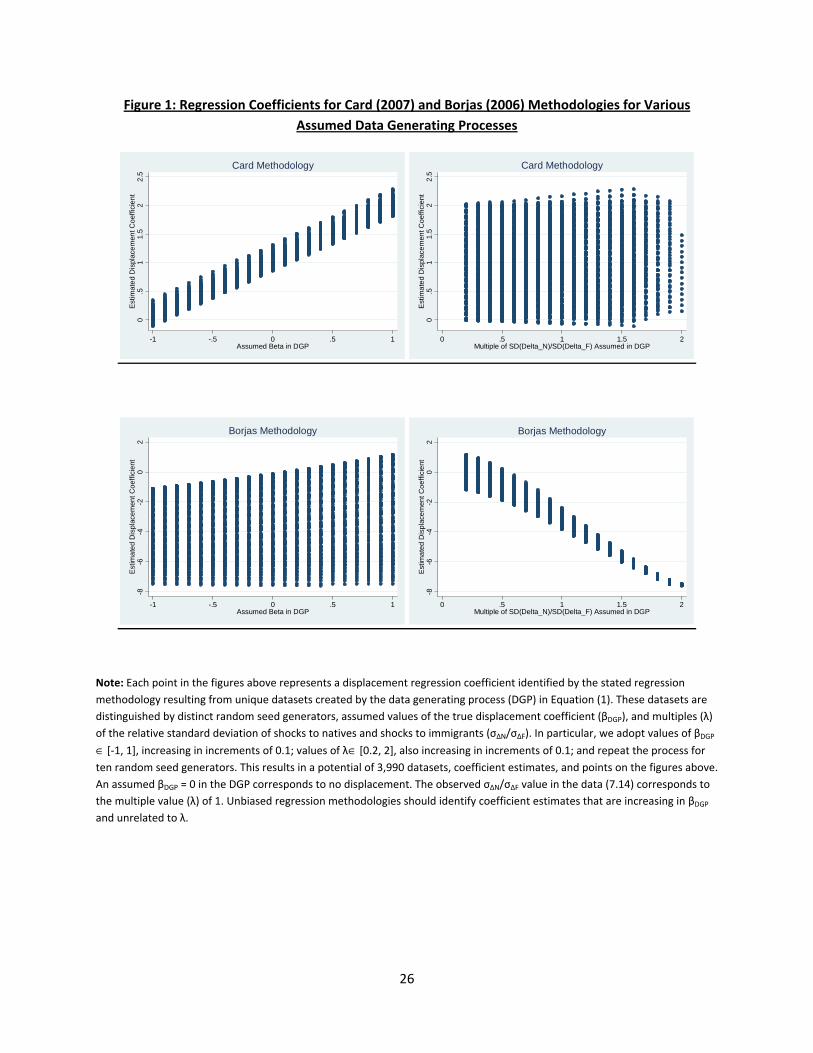
A graphical analysis of the assumed data generating process and the regression results is even more

illustrative. We do this by first generating several unique datasets. Each is defined by an assumed

value of ∈ [−1 1], increasing by units of 0.1, and an assumed multiple of the standard deviation of∆ relative to that of ∆ . We represent this multiple by ∈ [02 2] and also increase it by units of0.1. We repeat these steps for ten set random seed generators. This results in 3,990 unique datasets

from which we drop the 665 datasets that predict one or more negative values for or .

Figure 1 displays four scatter-plots. The top two evaluate the Card (2007) methodology, and the

bottom two illustrate the baseline Borjas (2006) specification. The horizontal axis in the left two

graphs represents the value assumed by the data generating process, while the horizontal axis in the

right two charts represents the assumed multiple of the observed relative standard deviation. Recall

13

that = 0 implies zero displacement and = 1 represents the observed relative standard deviation

value of 7.14. Each dot in the scatter-plot then represents the unique coefficient estimate for the

relevant specification determined by , , and the random seed generator.

At a minium, a methodology for examining displacement should deliver coefficient estimates that

increase in the assumed value. Better methodologies would exhibit small variation in the estimates

for a given . Moreover, estimates should be insensitive to assumptions regarding the relative standard

deviation of∆ . The two top panels of Figure 1 clearly demonstrate that the Card (2007) methodology

meets these criteria. The top-left figure shows that as varies, estimates of cluster around

(1 + ). This implies that displacement conclusions in Card ( 1) are usually associated

with displacement in the data ( 0). The top-right figure also shows that the estimates of bare centered around one for = 0 no matter what value is taken by the standard deviation of

∆ . The corresponding graphs for Borjas (2006), in contrast, show that b1 is almost alwaysnegative even when 0. When the relative standard deviation of ∆ rises, the estimates ofb1 are more likely to be negative in sign, larger in magnitude, and increasingly precise.3.3.2 Number of Cells

A secondary issue might involve the size and number of cells. The advantage of small cells is that it

minimizes heterogeneity within cells when using real data. The disadvantage is that it reduces the

number of available observations while potentially increasing the risk of heavy influence from single

outliers. We explore the consequences of cell size by employing an alternative data generating process

that reduces the number of skill groups from 32 to just 2 (“high” and “low” education groups, for

example). We create data similar to the procedure described above, except that we increase in initial

cell size to 2,000,000, and we change the sampling procedure to match the appropriate moments in

the observed data. Using these smaller cells, the observed mean and standard deviation of ∆ are

(104,863; 192,159), while the corresponding values for ∆ are (16,747; 32,378).

Table 4 presents results analogous to those in Tables 1 and 2, using fixed effects when appropriate.

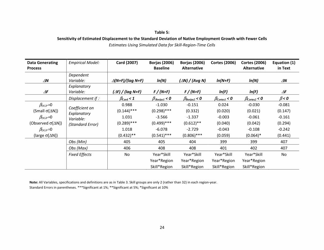
Table 5 examines the consequences of varying the standard deviation of ∆ in this smaller sample

with larger size cells. Both tables support the prior conclusions. Most regressions correctly identify the

correlation between immigration and internal native migration, but the Borjas specifications exhibit

14

a negative bias that grows as the standard deviation of ∆ increases.13

4 Empirical Results Using Observed Data

Wolf (2001, page 317) argues that if “microsimulation output produces a finding that is sharply at odds

with known [i.e., simulated] facts, then. . . one must return to the model, prepared to respecify it.”

Section 3 identified inherent biases in several models that have been employed by economists to assess

the displacement effects of immigration. Of course, these biases would have been unknown to analysts,

thus preventing them from respecifying their models if necessary. In this section, we assess how each of

the previously-described model specifications performs when using observed — rather than simulated

— data. We neither advocate nor produce exact replication of prior work, as the analyses substantially

differ along a number of dimensions (e.g., sample selection, the time period of analysis, the definition

of cells used in the regressions, etc.). However, the use of observed data within the methodological

framework of past studies should still be informative about the differences in displacement conclusions

that have emerged in the literature.

Table 6 presents the results for these regressions. The data represents a panel of 51 “state” by 32

skill-group cells in each of four Census years (1970-2000) for a total of 6528 observations. Standard

errors are clustered at the skill-state level since actual data may be correlated within cells over time.

The estimates reported in the two rows of Table 6 are distinguished solely by whether or not the

regressions include fixed effects. None of the specifications employ instrumental variables to control

for endogeneity, so one should be cautious in ascribing a causal role in correlative relationships. These

regressions simply reveal the correlation in the data, with and without controlling for an array of fixed

effects.

In the absence of fixed effects, Borjas regressions argue for displacement, while all other specifi-

cations suggest a positive relationship between immigration and native employment. The inclusion

of fixed effects reduces the magnitudes of each coefficient. This supports the larger point in Bor-

jas (2006) — regressions exploring native internal migration should account for initial conditions and

trends. Otherwise results will be biased. It is important to add, however, that only Borjas’s baseline

specification continues to find a significantly negative relationship between immigration and native

13Note that the standard deviation of ∆ is seven times larger than that of ∆ when using the less-aggregated

state-skill cells, and is six times larger when using more-aggregated cells. This similarity in relative variation might be

one reason why the Borjas magnitudes in Tables 3 and 5 are similar.

15

internal migration once fixed effects are included. The other specifications either identify attraction

or neither displacement nor attraction. Given the inherent negative bias uncovered in the Borjas’

specifications, we believe that there is no evidence for a true displacement effect. The correlation

evidence, at least prima facie, does not support displacement.

In choosing a preferred specification, we might be inclined to advocate something like Card’s

(2007) methodology — Equation (4) — but with the following modification: Replace the dependent

variable³−−1−1

´with

³−−1−1

´ First, this would lead to coefficient estimates that are exactly

one less than the Card (2007) estimates provided in this (and his) paper and would provide a more

direct test of displacement. That is, the coefficient would translate directly into the number of native

employees who respond to one extra immigrant worker in the group. Second, the model would not be

affected by cell size, nor it would force any artificial correlation between the dependent and explanatory

variables. Third, it is even more demanding than (5) in controlling for pre-determined trends of native

employment growth since it expresses the variables in differences, not levels, and still controls for an

array of fixed effects. The identifying variation therefore comes from deviations of growth rates from

skill-state specific trends. Finally, the regression can employ observations in which or equal

zero, unlike natural log specifications. Such a specification (including all fixed effects and using the

US state-skill data) would generate a significant coefficient of 1.361 and suggest a strong attraction

between immigrants and natives.

5 Conclusions

The debate on the labor market effects of immigration is important from an academic and policy

point of view. It is essential that we have a good understanding of the potential crowding-out of

native workers that immigrants might cause. Analysis of the correlation between immigrant and

native employment within skill-state groups over time might be able to provide or deny support to

the crowding out theory. Should displacement exist, then not only would immigration decrease native

employment opportunities, but cross-region analyses of the wage effects of immigration would be

invalid. In particular, the negative wage consequences of immigration would be much more severe

than the small effects found by area studies if displacement occurs. As recent papers find different

answers to this question using similar data but different empirical methodologies, this paper aims at

explaining where these differences come from.

16

We generated several artificial datasets and then used them to explore whether different regression

specifications are able to robustly and correctly identify the native displacement consequences of

immigration. Some models (notably Card 2007) performed well and correctly uncovered negative

relationships when displacement was assumed in the data generating process, while also identifying a

positive relationship when native attraction to immigration was assumed. Borjas (2006) specifications,

however, exhibited a strong bias toward displacement. This is likely due to an inherent and mechanical

bias created by including a measure of native employment in the denominator of the explanatory

variable and in the numerator of the dependent variable. Further simulations support this conclusion

by showing that the bias becomes larger as the standard deviation of native employment changes

grows in relation to the standard deviation of immigration flows.

Regressions that use real data fail to uncover a significant relationship between immigration and

native migration, and instead mostly estimate no displacement and no attraction. The exceptions,

however, are Borjas (2006) specifications that systematically find displacement. Though we cannot

interpret the effects as causal, we believe that inherent bias in the Borjas specifications, coupled

with the consistency of results across alternative models, combine to provide no evidence in favor of

displacement. Our results therefore preserve the validity of other cross-region empirical analyses of

the effects of immigration.

17

References

Borjas, George. 1980. “The Relationship between Wages and Weekly Hours of Work: The Role of

Division Bias.” Journal of Human Resources 15, no. 3: 409-423.

Borjas, George. 2006. “Native Internal Migration and the Labor Market Impact of Immigration.”

Journal of Human Resources 41, no.2: 221-258.

Borjas, George, Richard B. Freeman, and Lawrence Katz. 1997. “How much Do Immigration and

Trade Affect Labor Market Outcomes?” Brookings Papers on Economic Activity 1, no. 1: 1-67.

Card, David. 1990. “The Impact of the Mariel Boatlift on the Miami Labor Market.” Industrial and

Labor Relations Review 43, no 2: 245-257.

Card, David. 2001. “Immigrant Inflows, Native Outflows, and the Local Labor Market Impacts of

Higher Immigration.” Journal of Labor Economics 19, no. 1: 22-64.

Card, David 2005 “Is The New Immigration Really So Bad?” Economic Journal, 2005, Volume 115,

pp.300.323.

Card, David. 2007. “How Immigration Affects U.S. Cities.” CReAM Discussion Paper, no. 11/07.

Card, David 2009. “Immigration and Inequality.”American Economic Review, Papers and Proceedings,

99:2, 1-21.

Card, David, and John DiNardo. 2000. “Do Immigrant Inflows Lead to Native Outflows?” NBER

Working Paper, no. 7578, Cambridge, Ma.

Card, David, and Ethan Lewis. 2007. “The Diffusion of Mexican Immigrants During the 1990s: Expla-

nations and Impacts.” In Borjas, George, editor Mexican Immigration to the United States. National

Bureau of Economic Research Conference Report, Cambridge MA.

Cortes, Patricia. 2006. “The Effect of Low-Skilled Immigration on US Prices: Evidence from CPI

Data.” Ph.D. Dissertation. Massachusetts Institute of Technology, Cambridge, MA.

Cortes, Patricia. 2008. “The Effect of Low-Skilled Immigration on US Prices: Evidence from CPI

Data.” Journal of Political Economy 116, no. 3: 381-422.

18

Lewis, Ethan 2005. “Immigration, Skill Mix, and the Choice of Technique.” Federal Reserve Bank of

Philadelphia Working Paper #05-08, May 2005.

Longhi, Simonetta, Peter Nijkamp, and Jacques Poot. 2008. “Meta-Analysis of Empirical Evidence on

the Labour Market Impacts of Immigration.” IZA Discussion Paper 3418, Institute for the Study of

Labor (IZA).

Hanson, Gordon H. 2008. “The Economic Consequences of the International Migration of Labor.”

NBER Working Paper 14490, National Bureau of Economic Research.

Ottaviano, Gianmarco, and Giovanni Peri. 2007. “The Effect of Immigration on U.S. Wages and Rents:

A General Equilibrium Approach.” CReAM Discussion Paper no 13/07 London, UK.

Ottaviano, Gianmarco I.P. and Peri Giovanni 2008. “Immigration and National Wages: Clarifying the

Theory and the Empirics” NBER Working Paper 14188, July 2008.

Peri, Giovanni. 2009. “Rethinking the Area Approach: Immigrants and the Labor Market in California,

1960-2005.” Manuscript. UC Davis, Davis CA.

Peri, Giovanni, and Chad Sparber. 2009. “Task Specialization, Immigration, and Wages.” American

Economic Journal: Applied Economics, American Economic Association, Vol. 1(3): 135-69.

Ruggles, Steven , Matthew Sobek, Trent Alexander, Catherine A. Fitch, Ronald Goeken, Patricia

Kelly Hall, Miriam King, and Chad Ronnander (2005). Integrated Public Use Microdata Series: Ver-

sion 3.0 [Machine-readable database]. Minneapolis, MN: Minnesota Population Center [producer and

distributor], 2004. http://www.ipums.org.

Wolf, Douglas A. 2001. “The Role of Microsimulation in Longitudinal Data Analysis.” Canadian

Studies in Population, Vol. 28(2): 313-339.

19

20

Table 1: Empirical Models for Identifying Internal Migration Response

Estimates Using Simulated Data for Skill-Region-Time Cells Data

Generating Process

Empirical Model: Card (2007) Borjas (2006) Baseline

Borjas (2006) Alternative

Cortes (2006) Cortes (2006) Alternative

Equation (1) in Text

ΔN Dependent Variable: Δ(N+F)/(lag N+F) ln(N) (ΔN) / (Avg N) ln(N+F) ln(N) ΔN

ΔF Explanatory Variable: (ΔF) / (lag N+F) F / (N+F) F / (N+F) ln(F) ln(F) ΔF

βDGP Displacement if : βCard < 1 β Borjas1 < 0 βBorjas2 < 0 βCortes1 < 0 βCortes2 < 0 β < 0 -1 Coefficient on

Explanatory Variable: (Standard Error)

-0.056 -3.626 -1.572 0.029 -0.035 -1.005 (Displacement) (0.089) (0.079)*** (0.053)*** (0.006)*** (0.006)*** (0.088)***

-0.5 0.430 -3.415 -1.479 0.058 -0.005 -0.505 (Displacement) (0.089)*** (0.083)*** (0.055)*** (0.006)*** (0.006) (0.089)***

0 0.902 -3.168 -1.382 0.087 0.026 -0.030 (No effect) (0.090)*** (0.087)*** (0.056)*** (0.006)*** (0.006)*** (0.089)

0.5 1.376 -2.884 -1.261 0.116 0.057 0.458 (Attraction) (0.089)*** (0.091)*** (0.058)*** (0.006)*** (0.006)*** (0.089)***

1 1.854 -2.554 -1.140 0.144 0.088 0.949 (Attraction) (0.089)*** (0.095)*** (0.061)*** (0.006)*** (0.006)*** (0.088)***

Obs (Min) 6475 6432 6434 6426 6422 6500 Obs (Max) 6481 6438 6445 6433 6426 6503 Fixed Effects No No No No No No

Note: Results from regressions employing data generated from the process described in Equation (1) of the text. The values of βDGP = {-1, -0.5, 0, 0.5, 1} used are reported in the first column. Immigrants are said to displace natives if βDGP <0, and attract natives if βDGP >0. Each column uses a different empirical model for identifying displacement, identified in the first three rows of the column. Each cell represents a coefficient estimate from the regression specification of the column’s methodology when the βDGP value in the corresponding row is used in the data generating process (DGP). The final column, as a check, uses the DGP’s regression specification. Units of observations are skill-state cells. There are 32 skill levels, 51 regions and 4 years. ***Significant at 1%; **Significant at 5%; *Significant at 10%

21

Table 2: Empirical Models for Identifying Internal Migration Response, Adding Fixed Effects


Generating Process









0.151 -3.746 -2.214 -0.015 -0.082 -0.906 (Displacement) (0.105) (0.082)*** (0.109)*** (0.007)** (0.007)*** (0.103)***

-0.5 0.638 -3.525 -2.044 0.016 -0.050 -0.402 (Displacement) (0.106)*** (0.087)*** (0.112)*** (0.007)** (0.007)*** (0.104)***

0 1.111 -3.266 -1.865 0.047 -0.017 0.064 (No effect) (0.106)*** (0.092)*** (0.116)*** (0.007)*** (0.007)** (0.104)

0.5 1.594 -2.982 -1.657 0.078 0.016 0.550 (Attraction) (0.106)*** (0.098)*** (0.121)*** (0.007)*** (0.007)** (0.104)***

1 2.081 -2.640 -1.431 0.108 0.050 1.037 (Attraction) (0.105)*** (0.103)*** (0.125)*** (0.007)*** (0.007)*** (0.103)***

Obs (Min) 6475 6432 6434 6426 6422 6500 Obs (Max) 6481 6438 6445 6433 6426 6503 Fixed Effects Year*Skill Year*Skill Year*Skill Year*Skill Year*Skill Year*Skill Year*Region Year*Region Year*Region Year*Region Year*Region Year*Region

Skill*Region Skill*Region Skill*Region Skill*Region Skill*Region Skill*Region Note: All Variables, specifications and definitions are as in Table 1. Year by Skill, Year by region and Skill by region effects are included in all regressions. ***Significant at 1%; **Significant at 5%; *Significant at 10%

22

Table 3:

Sensitivity of Estimated Displacement to the Standard Deviation of Native Employment Growth Estimates Using Simulated Data for Skill-Region-Time Cells

Data Generating

Process Empirical Model: Card (2007) Borjas (2006)

Baseline Borjas (2006) Alternative




ΔF Explanatory Variable: (ΔF) / (lag N+F) F / (N+F) F / (N+F) ln(F) ln(F) ΔF Displacement if : βCard < 1 β Borjas1 < 0 βBorjas2 < 0 βCortes1 < 0 βCortes2 < 0 β < 0

βDGP=0 Coefficient on Explanatory Variable: (Standard Error)

0.953 -1.056 -0.584 0.054 -0.007 -0.015 (Small σ[ΔN]) (0.045)*** (0.055)*** (0.065)*** (0.003)*** (0.004)** (0.045)

βDGP=0 0.902 -3.266 -1.865 0.047 -0.017 -0.030 (Observed σ[ΔN]) (0.090)*** (0.092)*** (0.116)*** (0.007)*** (0.007)** (0.089)

βDGP=0 0.870 -5.646 -3.219 0.038 -0.027 -0.045 (large σ[ΔN]) (0.134)*** (0.107)*** (0.149)*** (0.010)*** (0.011)** (0.134)

Obs (Min) 6458 6417 6412 6414 6407 6500 Obs (Max) 6489 6474 6481 6446 6442 6500 Fixed Effects No Year*Skill Year*Skill Year*Skill Year*Skill No Year*Region Year*Region Year*Region Year*Region

Skill*Region Skill*Region Skill*Region Skill*Region Note: Variables, specifications and definitions in the Empirical Models are as in Table 1. The data generating process, described in the first column maintains the value of βDGP=0

while it modifies the standard deviation of the native employment changes, σ[ΔN] in each of the three rows. The middle row assumes σΔN/σΔF equals its observed value (7.14), the top row assumes it equal to 3.57 (half of the observed value), and the bottom row assumes it equal to 14.28 (twice the observed value) Standard Errors in parentheses. ***Significant at 1%; **Significant at 5%; *Significant at 10%

23

Table 4: Sensitivity of Estimated Displacement to the Number of Cells


Generating Process









0.060 -3.873 -1.670 -0.053 -0.118 -1.038 (Displacement) (0.284) (0.443)*** (0.564)*** (0.038) (0.041)*** (0.285)***

-0.5 0.546 -3.698 -1.515 -0.027 -0.088 -0.539 (Displacement) (0.287)* (0.473)*** (0.588)** (0.039) (0.042)** (0.289)*

0 1.031 -3.566 -1.337 -0.003 -0.061 -0.161 (No effect) (0.289)*** (0.499)*** (0.612)** (0.040) (0.042) (0.294)

0.5 1.514 -3.425 -1.136 0.026 -0.034 0.339 (Attraction) (0.288)*** (0.519)*** (0.631)* (0.040) (0.043) (0.293)

1 1.997 -3.120 -0.900 0.055 -0.003 0.841 (Attraction) (0.285)*** (0.548)*** (0.656) (0.040) (0.042) (0.290)***


Skill*Region Skill*Region Skill*Region Skill*Region

Note: All Variables, specifications and definitions are as in Table 1. Skill groups are only 2 (rather than 32) in each region-year. ***Significant at 1%; **Significant at 5%; *Significant at 10%

24

Table 5: Sensitivity of Estimated Displacement to the Standard Deviation of Native Employment Growth with Fewer Cells

Estimates Using Simulated Data for Skill-Region-Time Cells

Data Generating Process






ΔF Explanatory Variable: (ΔF) / (lag N+F) F / (N+F) F / (N+F) ln(F) ln(F) ΔF Displacement if : βCard < 1 β Borjas1 < 0 βBorjas2 < 0 βCortes1 < 0 βCortes2 < 0 β < 0

βDGP=0 Coefficient on Explanatory Variable: (Standard Error)

0.988 -1.030 -0.151 0.024 -0.030 -0.081 (Small σ[ΔN]) (0.144)*** (0.298)*** (0.332) (0.020) (0.021) (0.147)

βDGP=0 1.031 -3.566 -1.337 -0.003 -0.061 -0.161 (Observed σ[ΔN]) (0.289)*** (0.499)*** (0.612)** (0.040) (0.042) (0.294)

βDGP=0 1.018 -6.078 -2.729 -0.043 -0.108 -0.242 (large σ[ΔN]) (0.432)** (0.541)*** (0.806)*** (0.059) (0.064)* (0.441)


Skill*Region Skill*Region Skill*Region Skill*Region

Note: All Variables, specifications and definitions are as in Table 3. Skill groups are only 2 (rather than 32) in each region-year. Standard Errors in parentheses. ***Significant at 1%; **Significant at 5%; *Significant at 10%

25

Table 6: Empirical Models Estimates of Internal Migration Response

Estimates Using Observed Data for 32 Skills in 51 US States in Years 1970, 1980, 1990 and 2000





Dependent Variable:

Δ(N+F)/(lag N+F) ln(N) (ΔN) / (Avg N) ln(N+F) ln(N) ΔN

Explanatory Variable:

(ΔF) / (lag N+F) F / (N+F) F / (N+F) ln(F) ln(F) ΔF

Displacement if : βCard < 1 β Borjas1 < 0 βBorjas2 < 0 βCortes1 < 0 βCortes2 < 0 β < 0

Coefficient on Explanatory Variable: (Standard Error)

No Fixed Effects 3.288 -0.551 -1.692 0.425 0.396 1.397 (0.527)*** (0.277)** (0.054)*** (0.009)*** (0.009)*** (0.234)*** Full Fixed Effects 2.361 -0.406 -0.363 0.022 0.009 1.166

(0.871)*** (0.093)*** (0.090)*** (0.004)*** (0.004)** (0.436)*** Observations 6528 6528 6528 6528 6528 6528

Note: OLS results from regressions employing observed decennial data from 1970-2000, 51 states, and 32 education*experience skill-cells. Each column represents a different methodology for identifying displacement and is identified by the column header. Regression in the top column present results without fixed effects. Regressions in the second row present results with year, skill, region, year*skill, year*region, and skill*region fixed effects. Cells represent unique coefficient estimates given by the regression specification of the column’s methodology and the exclusion/inclusion of fixed effects as indicated by rows. Standard Errors in parentheses are cluster-robust at the skill-state level. ***Significant at 1%; **Significant at 5%; *Significant at 10%

26

Figure 1: Regression Coefficients for Card (2007) and Borjas (2006) Methodologies for Various Assumed Data Generating Processes

Note: Each point in the figures above represents a displacement regression coefficient identified by the stated regression methodology resulting from unique datasets created by the data generating process (DGP) in Equation (1). These datasets are distinguished by distinct random seed generators, assumed values of the true displacement coefficient (βDGP), and multiples (λ) of the relative standard deviation of shocks to natives and shocks to immigrants (σΔN/σΔF). In particular, we adopt values of βDGP ∈ [-1, 1], increasing in increments of 0.1; values of λ∈ [0.2, 2], also increasing in increments of 0.1; and repeat the process for ten random seed generators. This results in a potential of 3,990 datasets, coefficient estimates, and points on the figures above. An assumed βDGP = 0 in the DGP corresponds to no displacement. The observed σΔN/σΔF value in the data (7.14) corresponds to the multiple value (λ) of 1. Unbiased regression methodologies should identify coefficient estimates that are increasing in βDGP and unrelated to λ.

0.5

11.

52

2.5

Estim

ated

Dis

plac

emen

t Coe

ffici

ent

-1 -.5 0 .5 1Assumed Beta in DGP

Card Methodology

0.5

11.

52

2.5

Est

imat

ed D

ispl

acem

ent C

oeffi

cien

t

0 .5 1 1.5 2Multiple of SD(Delta_N)/SD(Delta_F) Assumed in DGP

Card Methodology

-8-6

-4-2

02

Est

imat

ed D

ispl

acem

ent C

oeffi

cien

t

-1 -.5 0 .5 1Assumed Beta in DGP

Borjas Methodology-8

-6-4

-20

2Es

timat

ed D

ispl

acem

ent C

oeffi

cien

t

0 .5 1 1.5 2Multiple of SD(Delta_N)/SD(Delta_F) Assumed in DGP

Borjas Methodology

Giovanni Peri and Chad Sparber - National Bureau of ... Inherent Model Bias: An Application to...

Documents

Transcript of Giovanni Peri and Chad Sparber - National Bureau of ... Inherent Model Bias: An Application to...