Geophysical Journal International - ISTerre de G´eophysique Interne et de Tectonophysique (LGIT),...

Geophys. J. Int. (2009) 179, 1627–1644 doi: 10.1111/j.1365-246X.2009.04354.x

GJI

Sei

smol

ogy

New approach for coupling k−2 and empirical Green’s functions:application to the blind prediction of broad-band ground motionin the Grenoble basin

Mathieu Causse, Emmanuel Chaljub, Fabrice Cotton, Cecile Cornouand Pierre-Yves BardLaboratoire de Geophysique Interne et de Tectonophysique (LGIT), CNRS, Universite Joseph Fourier, Observatoire des Sciences de l’Univers de Grenoble,Institut de recherche pour le Developpement, Laboratoire Central des Ponts-et-Chaussees, France. E-mail: [email protected]

Accepted 2009 August 3. Received 2009 May 13; in original form 2008 June 2

S U M M A R YWe present a new approach for performing broad-band ground motion time histories (0.1–30 Hz) of a future earthquake in a sedimentary basin. Synthetics are computed with anhybrid scheme combining reciprocity-based 3-D-spectral element method simulations at lowfrequencies and empirical Green’s functions (EGF) at high frequencies. The combinationbetween both deterministic and empirical parts results in a set of hybrid Green’s functions,summed according to a new k−2 kinematic model algorithm. The summation technique enablesto remove the high-frequency artefacts that appear above the EGF corner frequency. Theground motion variability is assessed by generating a variety of source parameter sets selectedfrom a priori probability density functions. This leads to a population of response spectra,from which the median spectral acceleration and standard deviation values are derived. Themethod is applied to simulate a MW 5.5 event in the deep Grenoble basin (French Alps). Thecomparison with EC8 regulations suggests the need of specific design spectra in the Grenoblevalley.

Key words: Earthquake ground motions; Site effects; Europe.

I N T RO D U C T I O N

Synthesizing time histories of ground motion in urban areas isuseful to design specific structures and to estimate potential dam-ages for a future earthquake. This is particularly true in Euro-pean alpine valleys where moderate earthquakes may have largeconsequences caused by large 2-D/3-D site effects. The Grenoblecity is a typical example of alpine valley: first, historic seismicityshows the possibility of MW 5.5 events at the vicinity of the city(≈20 km); second, this deep sedimentary valley exhibits large com-plex site effects (Lebrun et al. 2001; Cornou et al. 2003; Gueguenet al. 2006b; Drouet et al. 2007). In order to analyse seismic haz-ard in the Grenoble valley, a MW 5.5 scenario earthquake occur-ring on the Belledonne border fault south of the city is assumed(Thouvenot et al. 2003). The source proximity makes it necessaryto use a finite-extent source description. The ground motion pre-dictions are thus performed with a new approach coupling the k−2

source model (Herrero & Bernard 1994) and hybrid Green’s func-tions (HGF), that incorporate 3-D site effects. This new procedureprovides an estimation of the ground motion variability.

Ground motion characteristics are strongly affected by the ve-locity structure. The lack of detailed knowledge of the propaga-

tion medium makes it usually difficult to use numerical methodsfor estimating ground motion at high frequency (generally above1–2 Hz). An alternative approach is then the empirical Green’sfunctions (EGF) method (Hartzell 1978), when good quality smallearthquake recordings are available. This method automatically in-cludes propagation and site effects, under the assumption of thesoil response linearity. Nevertheless it is inadequate for assessinglow-frequency ground motion, because of the often bad signal-to-noise ratio in the small event recordings below 1 Hz. Thus, severalauthors (Kamae et al. 1998; Pulido & Kubo 2004; Pacor et al.2005) proposed to calculate broad-band ground motion with a hy-brid scheme combining deterministic and stochastic approaches:low-frequency Green’s functions are evaluated by numerical algo-rithms whereas high-frequency Green’s functions are obtained fromfiltered white noise. In this paper, a hybrid method is also pro-posed. First, low-frequency ground motion (<1 Hz) is modelledwith 3-D spectral element method (Komatitsch & Vilotte 1998;Komatitsch & Tromp 1999; Komatitsch et al. 2004; Chaljub et al.2007) calculations based on reciprocity. Second, the good qual-ity recordings of a ML 2.8 earthquake provided by the 2005Grenoble experiment (Chaljub et al. 2006) and the French perma-nent accelerometric network (http://www-rap.obs.ujf-grenoble.fr),

C© 2009 The Authors 1627Journal compilation C© 2009 RAS

Geophysical Journal International

1628 M. Causse et al.

are used as EGFs to simulate high-frequency ground motion(1–30 Hz). The advantage of such a combination is that both meth-ods are adequate for simulating specific site effects.

In addition, in the relevant frequency range for earthquake engi-neering and within a few fault lengths, ground-motion simulationshighly depend on the rupture process complexity. Thanks to itsease of application, kinematic modelling remains the best way toperform physically based ground motion predictions. Moreover,Hartzell et al. (2005) compared a class of kinematic models basedon fractal distribution of subevent sizes with a simple slip-weakening dynamic model and concluded that at present the kine-matic simulations match better the 1994 Northridge ground motionthan the dynamic ones. A now classical approach is a self-similarrupture model in which the spatial static slip distribution is describedin the wavenumber domain by a k−2 power-law decay (Herrero &Bernard 1994; Bernard et al. 1996). This model leads to the com-monly observed ω−2 displacement amplitude spectrum decay underthe two constraints that the rupture front propagates with a constantrupture velocity and that the rise time is inversely proportional tothe wavenumber k. Ground motion is next computed by summingup the HGF according to a k−2 source model. In order to couplek−2 model and the EGF method, a specific summation algorithmis developed. It enables to correct the high-frequency artefacts thatappear above the EGF corner frequency. Finally, source parame-ters are defined with probability density functions and the resultingground motion variability is assessed by means of the Latin Hy-percube Sampling (LHS) method. The ground motion sensitivityto source parameters and to EGF uncertainties is thoroughly inves-tigated. As a result, median and standard deviation of the spec-tral acceleration (SA) are predicted on nine stations within theGrenoble valley in the frequency range [0.1–30 Hz]. In order totest the reliability of the ground motion predictions, simulations onrock station are compared to the empirical ground motion equationsdeveloped by Bragato & Slejko (2005) and to the stochastic methodof Pousse et al. (2006). The comparison of the predictions at sed-iments stations with Eurocode eight suggests the need of specificdesign spectra in the framework of the Grenoble basin.

S O U RC E M O D E L

Static slip distribution

The complexity of the static slip is described with a self-similardistribution of slip heterogeneities. Following Herrero & Bernard(1994) the static slip is supposed to have a k−2 asymptotic de-cay in the wavenumber domain beyond the corner wavenumber kc,inversely proportional to the ruptured fault dimension. For a rect-angular fault plane with length L and width W we define the slipamplitude spectrum in a way similar to Somerville et al. (1999) andGallovic & Brokesova (2004)

Dk(kx , ky) = DLW√1 +

[(kx LK

)2+

(ky W

K

)2]2

, (1)

where kx and ky are the wavenumbers along the strike and thedip directions, respectively, D refers to the mean slip and Kis a dimensionless constant controlling the corner wavenumberkc = K/

√(L2 + W 2). The parameter K is fundamental because

it determines the amplitude of the slip heterogeneities generatingthe high-frequency source energy. At low wavenumber [k2

x + k2y ≤

(1/L)2 + (1/W )2] the slip spectrum phases are chosen to concen-trate the slip on the fault centre whereas for high wavenumbers,phases are random. Consequently, the static slip is the sum of a de-terministic and a stochastic part. The deterministic part of the slipgenerates a smooth asperity with mean slip D, the size of whichdepends on the corner wavenumber, that is, the dimensionless pa-rameter K. Large values of K lead to a small asperity. The mainasperity is then added to the high wavenumber slip contributions,corresponding to a set of zero mean slip heterogeneities. This leadsto a variety of heterogeneous slip models. All the details to generatethe static slip distributions can be found in Appendix A.

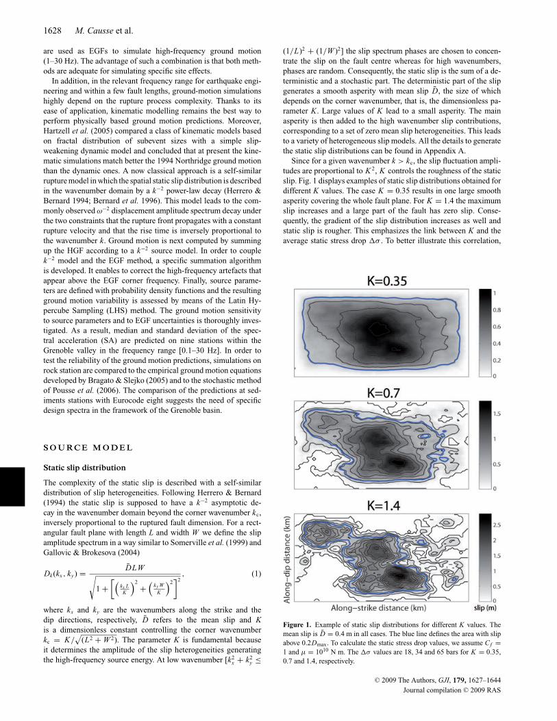
Since for a given wavenumber k > kc, the slip fluctuation ampli-tudes are proportional to K 2, K controls the roughness of the staticslip. Fig. 1 displays examples of static slip distributions obtained fordifferent K values. The case K = 0.35 results in one large smoothasperity covering the whole fault plane. For K = 1.4 the maximumslip increases and a large part of the fault has zero slip. Conse-quently, the gradient of the slip distribution increases as well andstatic slip is rougher. This emphasizes the link between K and theaverage static stress drop �σ . To better illustrate this correlation,

Figure 1. Example of static slip distributions for different K values. Themean slip is D = 0.4 m in all cases. The blue line defines the area with slipabove 0.2Dmax. To calculate the static stress drop values, we assume Cf =1 and μ = 1010 N m. The �σ values are 18, 34 and 65 bars for K = 0.35,0.7 and 1.4, respectively.

C© 2009 The Authors, GJI, 179, 1627–1644

Journal compilation C© 2009 RAS

New approach for coupling k−2 and EGFs 1629

we calculate �σ following Kanamori & Anderson (1975):

�σ = C f μD

L, (2)

where Cf is a non-dimensional shape factor (Cf ≈ 1 in all cases), μ isthe rigidity and L represents the characteristic length of the rupturearea. We define L as the square root of the main slip area, definedby the fault surface with slip over 20 per cent of the maximum slip.This simple test shows the average static stress drop increase withK (see legend of Fig. 1 for more details).

Source kinematics

Following Bernard et al. (1996), we model the rupture processas a ‘self-healing’ slip pulse of width L0 propagating at constantrupture velocity v. For wavenumbers k < 1

2L0, the rise time is

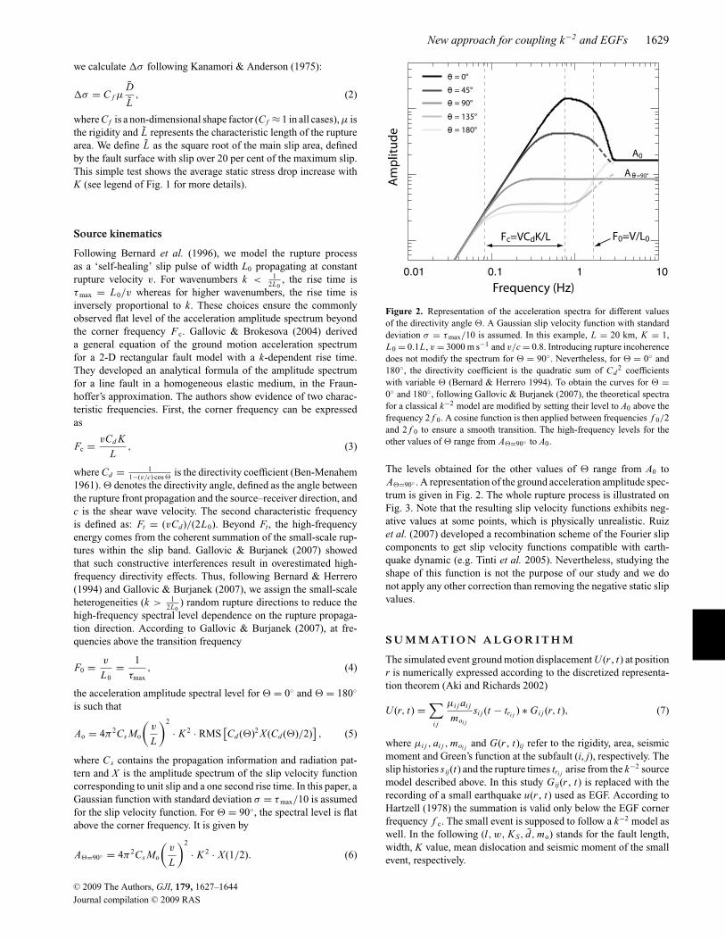
τmax = L0/v whereas for higher wavenumbers, the rise time isinversely proportional to k. These choices ensure the commonlyobserved flat level of the acceleration amplitude spectrum beyondthe corner frequency F c. Gallovic & Brokesova (2004) deriveda general equation of the ground motion acceleration spectrumfor a 2-D rectangular fault model with a k-dependent rise time.They developed an analytical formula of the amplitude spectrumfor a line fault in a homogeneous elastic medium, in the Fraun-hoffer’s approximation. The authors show evidence of two charac-teristic frequencies. First, the corner frequency can be expressedas

Fc = vCd K

L, (3)

where Cd = 11−(v/c) cos �

is the directivity coefficient (Ben-Menahem1961). � denotes the directivity angle, defined as the angle betweenthe rupture front propagation and the source–receiver direction, andc is the shear wave velocity. The second characteristic frequencyis defined as: Ft = (vCd)/(2L0). Beyond Ft, the high-frequencyenergy comes from the coherent summation of the small-scale rup-tures within the slip band. Gallovic & Burjanek (2007) showedthat such constructive interferences result in overestimated high-frequency directivity effects. Thus, following Bernard & Herrero(1994) and Gallovic & Burjanek (2007), we assign the small-scaleheterogeneities (k > 1

2L0) random rupture directions to reduce the

high-frequency spectral level dependence on the rupture propaga-tion direction. According to Gallovic & Burjanek (2007), at fre-quencies above the transition frequency

F0 = v

L0= 1

τmax, (4)

the acceleration amplitude spectral level for � = 0◦ and � = 180◦

is such that

Ao = 4π 2Cs Mo

(v

L

)2

· K 2 · RMS[Cd (�)2 X (Cd (�)/2)

], (5)

where Cs contains the propagation information and radiation pat-tern and X is the amplitude spectrum of the slip velocity functioncorresponding to unit slip and a one second rise time. In this paper, aGaussian function with standard deviation σ = τmax/10 is assumedfor the slip velocity function. For � = 90◦, the spectral level is flatabove the corner frequency. It is given by

A�=90◦ = 4π 2Cs Mo

(v

L

)2

· K 2 · X (1/2). (6)

Figure 2. Representation of the acceleration spectra for different valuesof the directivity angle �. A Gaussian slip velocity function with standarddeviation σ = τmax/10 is assumed. In this example, L = 20 km, K = 1,L0 = 0.1L , v = 3000 m s−1 and v/c = 0.8. Introducing rupture incoherencedoes not modify the spectrum for � = 90◦. Nevertheless, for � = 0◦ and180◦, the directivity coefficient is the quadratic sum of Cd

2 coefficientswith variable � (Bernard & Herrero 1994). To obtain the curves for � =0◦ and 180◦, following Gallovic & Burjanek (2007), the theoretical spectrafor a classical k−2 model are modified by setting their level to A0 above thefrequency 2 f 0. A cosine function is then applied between frequencies f 0/2and 2 f 0 to ensure a smooth transition. The high-frequency levels for theother values of � range from A�=90◦ to A0.

The levels obtained for the other values of � range from A0 toA�=90◦ . A representation of the ground acceleration amplitude spec-trum is given in Fig. 2. The whole rupture process is illustrated onFig. 3. Note that the resulting slip velocity functions exhibits neg-ative values at some points, which is physically unrealistic. Ruizet al. (2007) developed a recombination scheme of the Fourier slipcomponents to get slip velocity functions compatible with earth-quake dynamic (e.g. Tinti et al. 2005). Nevertheless, studying theshape of this function is not the purpose of our study and we donot apply any other correction than removing the negative static slipvalues.

S U M M AT I O N A L G O R I T H M

The simulated event ground motion displacement U (r , t) at positionr is numerically expressed according to the discretized representa-tion theorem (Aki and Richards 2002)

U (r, t) =∑

i j

μi j ai j

moi j

si j (t − tri j ) ∗ Gi j (r, t), (7)

where μi j , ai j , moi j and G(r , t)ij refer to the rigidity, area, seismicmoment and Green’s function at the subfault (i, j), respectively. Theslip histories sij(t) and the rupture times tri j arise from the k−2 sourcemodel described above. In this study Gij(r , t) is replaced with therecording of a small earthquake u(r , t) used as EGF. According toHartzell (1978) the summation is valid only below the EGF cornerfrequency f c. The small event is supposed to follow a k−2 model aswell. In the following (l, w, KS, d, mo) stands for the fault length,width, K value, mean dislocation and seismic moment of the smallevent, respectively.

C© 2009 The Authors, GJI, 179, 1627–1644



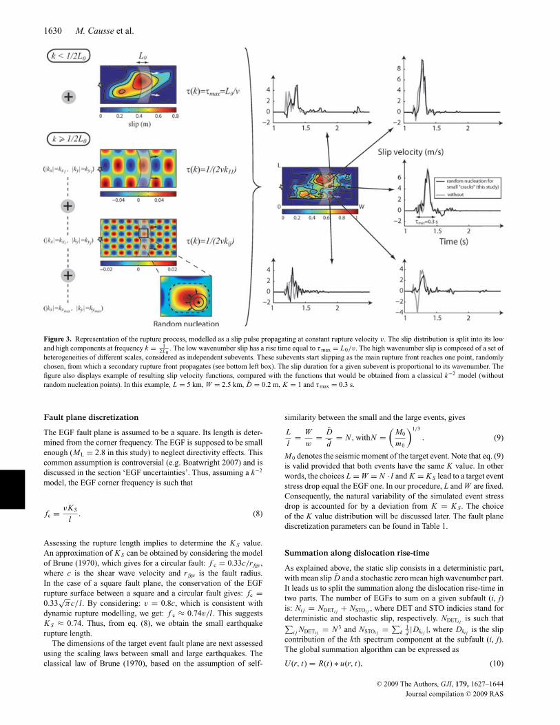
Figure 3. Representation of the rupture process, modelled as a slip pulse propagating at constant rupture velocity v. The slip distribution is split into its lowand high components at frequency k = 1

2L0. The low wavenumber slip has a rise time equal to τmax = L0/v. The high wavenumber slip is composed of a set of

heterogeneities of different scales, considered as independent subevents. These subevents start slipping as the main rupture front reaches one point, randomlychosen, from which a secondary rupture front propagates (see bottom left box). The slip duration for a given subevent is proportional to its wavenumber. Thefigure also displays example of resulting slip velocity functions, compared with the functions that would be obtained from a classical k−2 model (withoutrandom nucleation points). In this example, L = 5 km, W = 2.5 km, D = 0.2 m, K = 1 and τmax = 0.3 s.

Fault plane discretization

The EGF fault plane is assumed to be a square. Its length is deter-mined from the corner frequency. The EGF is supposed to be smallenough (ML = 2.8 in this study) to neglect directivity effects. Thiscommon assumption is controversial (e.g. Boatwright 2007) and isdiscussed in the section ‘EGF uncertainties’. Thus, assuming a k−2

model, the EGF corner frequency is such that

fc = vKS

l. (8)

Assessing the rupture length implies to determine the K S value.An approximation of K S can be obtained by considering the modelof Brune (1970), which gives for a circular fault: f c = 0.33c/r fge,where c is the shear wave velocity and r fge is the fault radius.In the case of a square fault plane, the conservation of the EGFrupture surface between a square and a circular fault gives: fc =0.33

√πc/ l. By considering: v = 0.8c, which is consistent with

dynamic rupture modelling, we get: f c ≈ 0.74v/l. This suggestsK S ≈ 0.74. Thus, from eq. (8), we obtain the small earthquakerupture length.

The dimensions of the target event fault plane are next assessedusing the scaling laws between small and large earthquakes. Theclassical law of Brune (1970), based on the assumption of self-

similarity between the small and the large events, gives

L

l= W

w= D

d= N , withN =

(M0

m0

)1/3

. (9)

M0 denotes the seismic moment of the target event. Note that eq. (9)is valid provided that both events have the same K value. In otherwords, the choices L = W = N · l and K = K S lead to a target eventstress drop equal the EGF one. In our procedure, L and W are fixed.Consequently, the natural variability of the simulated event stressdrop is accounted for by a deviation from K = K S . The choiceof the K value distribution will be discussed later. The fault planediscretization parameters can be found in Table 1.

Summation along dislocation rise-time

As explained above, the static slip consists in a deterministic part,with mean slip D and a stochastic zero mean high wavenumber part.It leads us to split the summation along the dislocation rise-time intwo parts. The number of EGFs to sum on a given subfault (i, j)is: Ni j = NDETi j + NSTOi j , where DET and STO indicies stand fordeterministic and stochastic slip, respectively. NDETi j is such that∑

i j NDETi j = N 3 and NSTOi j = ∑k

1d|Dki j |, where Dki j is the slip

contribution of the kth spectrum component at the subfault (i, j).The global summation algorithm can be expressed as

U (r, t) = R(t) ∗ u(r, t), (10)

C© 2009 The Authors, GJI, 179, 1627–1644



Table 1. Fault plane discretization and EGFparameters. N L, N W and N D denotes the EGFnumber to sum along the strike, the dip andthe dislocation rise time, respectively.

Parameters Value

M0 2.2 × 1017 N mm0 2.0 × 1013 N m

L/W 2f c 12 Hzl 0.160 km

N L 36N W 18N D 18

Target event strike 120◦EGF strike 160◦

Dip 90◦EGF focal depth 3 km

Notes: The seismic moments of the EGF andthe simulated event are directly obtainedfrom the moment magnitude. We assumethat local magnitude and moment magnitudeare the same for the EGF. The cornerfrequency f c is assessed from the EGFdisplacement amplitude spectrum.

where the site-dependent apparent source-time function (ASTF)R(t) is

R(t) =N∑

i=1

N∑j=1

r

ri j

⎡⎣NDETi j∑

q=1

δ(t − tri j − tsi j − tDETq )

+NSTOi j∑

q=1

p · δ(t − tri j − tsi j − tSTOq )

⎤⎦. (11)

The indice q denotes the summation along the dislocation rise time.The constant p is defined according to: p = 1 for Dki j > 0 and p =−1 for Dki j < 0. At last the term tsi j is introduced to account forthe different subfault/receiver S-wave traveltime delays and r/r ij isthe geometric spreading factor.

Summation process beyond the EGF corner frequency

Beyond f c the main event energy is purely stochastic because theEGF summation becomes incoherent. Hence the ASTF spectrallevel is flat and corresponds approximately to the square root of thetotal number of EGFs to sum up. Thus the resulting high-frequencylevel is not in agreement with the desired level for the source model.The theoretical level expected for f ≥ f c is �-dependent (seesection ‘Source kinematics’). However, for simplicity, we assumethat this level is the same whatever the value of � is. We thenset the acceleration spectrum level to its maximum value A0 (notethat after eqs (5) and (6), the largest error induced corresponds toa factor of A0/A�=90◦ ≈ 2). Consequently, the theoretical ASTFlevel is supposed to be (see Appendix B)

|R( f ≥ fc)theo| = βN K 2, (12)

where β ≈ 3.5.Following Kohrs-Sansorny et al. (2005), the number of EGFs to

sum along the dislocation rise time is modified to reproduce therequired high-frequency spectral level. The following procedure isproposed (see Appendix C): (1) the EGF dislocation d is adaptedso that the average number of EGF summed on each subfault is not

N but [ α(N )β

]2 · N 2

K 2 , where α(N ) = 2√

ln(

N−14

)and β ≈ 3.5; (2)

the deterministic slip contribution to the ASTF is low-pass filteredto keep only the zero mean slip fluctuations contributions beyondf c and (3) the spectrum is divided by [ β

α(N ) ]2 · K 2

N to conserve theseismic moment.

Resulting ASTF

Fig. 4(a) displays the effects of the above-described EGF summa-tion scheme correction on the average ASTF amplitude spectra.The spectra are calculated for an unilateral rupture and a rectangu-lar fault with L/W = 2. This fault ratio is in agreement with theresults of Somerville et al. (1999) and will be kept in the following.Fig. 4(a) shows that the high-frequency procedure based on theassumption of a square fault plane holds for L/W = 2 andthe target high-frequency level is reached. Note that in additionto the misestimation of the high-frequency spectral level, an othertype of numerical artefact appears due to the finite distances be-tween the small-event sources (Bour & Cara 1997). It correspondsto a peak occurring approximatively at: f p = vCd/l (Fig. 4b). Inorder to reduce this peak, a random component is introduced in therupture velocity v. v is thus uniformly distributed in the interval[v − 100 m s−1, v + 100 m s−1]. Are also shown the effects ofthe source (Figs 4c and d). These figures show that the main the-oretical characteristics of the amplitude spectrum for a line faultare preserved (i.e. corner frequencies, �, K and τmax-dependenceof the model). It should be noticed that R(f ) phases are necessar-ily stochastic beyond f c. Nevertheless this is consistent with therupture process that is purely stochastic above F0.

G R E E N ’ S F U N C T I O N S

EGFs

On 2005 October 1 a small earthquake occurred on the southern tipof the Belledonne border fault, about 15 km south of the Grenoblecity (ML = 2.8, Local magnitude Sismalp, http://sismalp.obs.ujf-grenoble.fr). This event has been recorded by the French accelero-metric permanent network and by a temporary array from the Frenchmobile network (INSU/CNRS), composed of velocimetric sensors(CMG40T, with a flat response from 20 to 60 s) and deployed inthe Grenoble city from 2005 June 15 to October 30 (Chaljub et al.2006). These good quality recordings provide an opportunity tosimulate the effects of a moderate sized earthquake with the EGFmethod. Velocities are first differentiated to get the ground acceler-ation. Twenty-seven three-component accelerograms are then usedas EGFs to compute ground motion at nine stations in the Grenoblecity (Fig. 5). Seven of the stations are installed on soft soil withinthe sediment-filled valley, while two are located at rock sites. Thehypothesized scenario is a MW 5.5 left-lateral strike slip event.The fault plane is supposed to be vertical with a strike of 120◦. Thesmall earthquake characteristics and the rupture plane discretiza-tion parameters are displayed in Table 1. Note that the strike of thesmall event (160◦) is different from that of the target event. Indeeda value of 120◦ seems more appropriate for a MW 5.5 scenario inthe Laffrey area (Thouvenot et al. 2003). In order to account fordifferences in focal mechanism, a simple procedure is applied tocorrect the EGF radiation pattern. It has been observed that theradiation pattern of small earthquakes is frequency dependent andcharacterized by a transition from the theoretical double-couple

C© 2009 The Authors, GJI, 179, 1627–1644



Figure 4. Average apparent source-time function spectra (quadratic mean of 100 simulated spectra) in the case of an unilateral rupture and a rectangular faultplane with L/W = 2. The parameters used to compute the spectra are in agreement with the Grenoble application. They are displayed at the bottom right. (a)Effect of the high-frequency spectral level correction. The dashed line in the zoomed box indicates the expected theoretical level. (b) Effect of the addition ofa random component to the rupture velocity. (c) Effect of the roughness parameter K. (d) Effect of the angle � and the rise time τmax. Frequencies f 0 and f ′

0

denotes the transition frequencies for τmax = 0.6 and 0.3 s, respectively. (e) Effect of removing the negative slip value.

radiation pattern at low frequencies to a totally isotropic radiationpattern at high frequencies (Satoh 2002). Following Pulido & Kubo(2004) we assume a radiation pattern with a linear variation from 1to 3 Hz between the theoretical double-couple radiation and a spher-ical radiation. We only consider the contributions of the SH and SVwaves. The theoretical radiation patterns FSH and FSV are given inAki and Richards (2002) (equations 4.90 and 4.91). To estimate thetake-off angle, an homogeneous medium is hypothesized. Finally,to assess the contributions of the SH and SV waves to the dif-ferent ground motion components, we assume a vertically incidentwave-field, which is the most plausible given the impedance contrast(≈4) between the bedrock and the sedimentary basin. This leads toa frequency-dependent factor used to correct the EGF amplitudespectrum. This factor equals 1 above 3 Hz and does not change thevertical component. The EW and NS-component modifications at

1 Hz do not exceed a factor of 5, except for station G15 for whicha change in the fault azimuth shifts from a maximum to a node ofthe SH radiation pattern, and the EW-component correction factorequals 0.05. The resulting EGF amplitude spectrum modification islarge but significantly improves the fit between the 3-D simulationand the EGFs (Fig. 6a).

EGF uncertainties

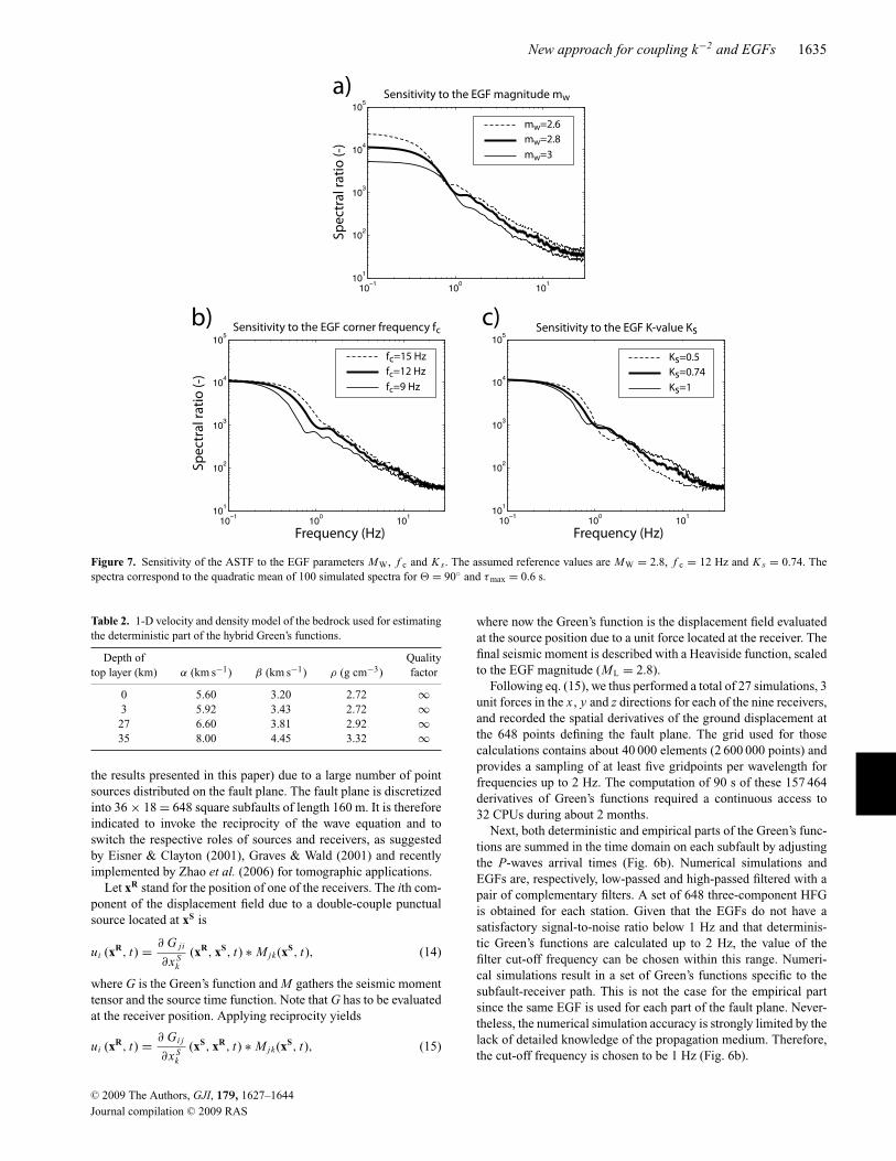
The small event input parameters (moment magnitude MW, cornerfrequency f c and K value K s) are only known with large uncertain-ties. Here we analyse the influence of a potential parameter valuemisestimation on the simulated ground motion. More precisely, thesensitivity to each EGF parameter is investigated by looking ASTF

C© 2009 The Authors, GJI, 179, 1627–1644



Figure 5. Map of the Grenoble valley, station and fault location.

changes when varying the given parameter around its supposedbest estimate value, while keeping the other parameters unchanged.First, the MW reference value is chosen by assuming mL = MW

for small events, which leads to MW = 2.8. A deviation of plus orminus 0.2 from the MW reference value results in a change of afactor 2 in the seismic moment value m0, and consequently, in thenumber of EGF to sum up. Therefore, the simulations are largelysensitive to the MW value at low frequency (Fig. 7a). Furthermore,the corner frequency controls the EGF rupture length l (eq. 8), andconsequently, the target event fault plane dimension. For instance,underestimating the f c value leads to increased rupture length Land decreased target event corner frequency f c. Since the numberof summed EGF is unchanged, the f c uncertainty does not con-cern the low-frequency and high-frequency expected spectral levels(Fig. 7b). Finally, Fig. 7(c) shows the effects of varying the K s value,assuming self-similarity between the small and the target events(K = K s). As f c is kept constant, changing K s also affects therupture lengths l and L.

In addition, it has been assumed that the small event is not af-fected by directivity effects. If this hypothesis is rejected, first, thesimple correction applied to account for the EGF fault strike modi-fication (initial estimated value of 160◦ set equal to 120◦, see section‘EGFs’) should also include a modification of f c. Nevertheless, theprocedure applied in this study to simulate ground motion abovef c ensure that the expected ASTF spectral level at f c is obtained,whatever the f c value is. Consequently, the particular EGF direc-tivity effects are not expected to significantly modify the simulationresults. Second, although the � values differ from one station tothe other (Fig. 5), the f c reference value has been set from the datarecorded at OGMU rock station and is supposed to be the samefor all the stations. However, the difference in the � values is notlarge. Thus, once again, this approximation is expected to bring onlyminor modifications on ground motion. Using several EGFs would

ensure that the potential small event directivity effects are averaged.However, in moderate seismicity area like the Grenoble basin, veryfew events are available.

HGFs

Since the EGFs have a satisfactory signal-to-noise ratio (>2) onlybeyond about 1 Hz, they are not adequate to simulate the low-frequency ground motion. Consequently, low frequencies are com-puted with the spectral element method (SEM) and combined inthe time domain with the EGFs to obtain a set of HGFs (Kamaeet al. 1998). The SEM is a high-order method that combines theability of finite element methods to handle 3-D geometries and theminimal numerical dispersion of spectral methods (Komatitsch &Vilotte 1998; Komatitsch & Tromp 1999). The reader is referred toChaljub et al. (2007), Komatitsch et al. (2004), Lee et al. (2008)and Chaljub (2009) for details about the application of the SEMto ground motion estimation in sedimentary basins or valleys. TheSEM is particularly well suited for ground motion estimation inalpine valleys because of its natural ability to account for free-surface topography and its accuracy to model the propagation ofsurface waves, such as those diffracted off the valley edges. Thenumerical prediction of ground motion with the SEM presentedhereafter have been carefully validated by comparison with thoseof other advanced 3-D methods, during the numerical benchmarkorganized within the 2006 symposium on the effects of surface ge-ology (ESG) on ground motion (Chaljub et al. 2009; Tsuno et al.2009).

Deterministic ground motion calculations implicitly assume thatthe 3-D structure (i.e. the positions of the physical interfaces, seis-mic wave velocities, densities, attenuation factors, etc.) is knownfrom the source region to the receivers. For the Grenoble area, weuse a simple 1-D model of the crust combined with a 3-D model

C© 2009 The Authors, GJI, 179, 1627–1644



Figure 6. (a) Effect of the EGF radiation pattern correction on the fitting between the deteministic and the empirical ground motion. (b) Principle of thelow-frequency ground motion simulation. 3D-simulations and EGFs are filtered and summed on each subfault to obtain a set of HGFs.

of the sedimentary valley. The crustal model is defined followingThouvenot et al. (2003) and given in Table 2.

The 3-D valley model is bounded by the sediment-bedrock in-terface obtained by Vallon (1999). Within the sedimentary cover,seismic velocities and densities are only allowed to vary with depthas⎧⎪⎨⎪⎩

a = 300.0 + 19.0 × √d,

b = 1450.0 + 1.2 × d,

ρ = 2140.0 + 0.125 × d,

(13)

where depth d is given in m, P (resp. S) velocities a (resp. b) in m s−1

and mass density ρ in kg m−3. Finally, we account for attenuationonly in the sediments by assuming a finite shear quality factorQμ = 50 and an infinite bulk quality factor Qκ .

The depth dependence of seismic velocities given by eq. (13)relies on direct measurements made for depths larger than 40 min a deep borehole drilled in 1999 in the eastern part of the valley

(Nicoud et al. 2002). It also matches closely the values derived froma refraction profile in the western part of the valley (Cornou 2002;Dietrich et al. 2009). This is consistent with the early geologicalhistory of the valley since the deep part of the sedimentary cover (i.e.below about −30 m) was formed by the sedimentation of postglaciallacustrine deposits, a smooth process that did not produce stronglateral variations. The shallower part, filled by the deposits of theIsere and Drac rivers, is known to be much more heterogeneous anda continuous effort is deployed to map these lateral variations intoa fully 3-D model of the valley. The 1-D model defined by eq. (13)provides a crude average of the shallow subsurface but it has beenshown to explain reasonably well the ground motion characteristicsfor frequencies below 1.5 Hz, in particular the level of amplificationbetween bedrock and sediments (Chaljub et al. 2004, 2005; Chaljub2009) and the ambient noise propagation properties (Cornou et al.2008).

In order to define the low frequency part of the HGFs, we needto compute the ground motion at a small number of stations (9 for

C© 2009 The Authors, GJI, 179, 1627–1644



Figure 7. Sensitivity of the ASTF to the EGF parameters MW, f c and K s. The assumed reference values are MW = 2.8, f c = 12 Hz and K s = 0.74. Thespectra correspond to the quadratic mean of 100 simulated spectra for � = 90◦ and τmax = 0.6 s.

Table 2. 1-D velocity and density model of the bedrock used for estimatingthe deterministic part of the hybrid Green’s functions.

Depth of Qualitytop layer (km) α (km s−1) β (km s−1) ρ (g cm−3) factor

0 5.60 3.20 2.72 ∞3 5.92 3.43 2.72 ∞27 6.60 3.81 2.92 ∞35 8.00 4.45 3.32 ∞

the results presented in this paper) due to a large number of pointsources distributed on the fault plane. The fault plane is discretizedinto 36 × 18 = 648 square subfaults of length 160 m. It is thereforeindicated to invoke the reciprocity of the wave equation and toswitch the respective roles of sources and receivers, as suggestedby Eisner & Clayton (2001), Graves & Wald (2001) and recentlyimplemented by Zhao et al. (2006) for tomographic applications.

Let xR stand for the position of one of the receivers. The ith com-ponent of the displacement field due to a double-couple punctualsource located at xS is

ui (xR, t) = ∂ G ji

∂x Sk

(xR, xS, t) ∗ M jk(xS, t), (14)

where G is the Green’s function and M gathers the seismic momenttensor and the source time function. Note that G has to be evaluatedat the receiver position. Applying reciprocity yields

ui (xR, t) = ∂ Gi j

∂x Sk

(xS, xR, t) ∗ M jk(xS, t), (15)

where now the Green’s function is the displacement field evaluatedat the source position due to a unit force located at the receiver. Thefinal seismic moment is described with a Heaviside function, scaledto the EGF magnitude (ML = 2.8).

Following eq. (15), we thus performed a total of 27 simulations, 3unit forces in the x , y and z directions for each of the nine receivers,and recorded the spatial derivatives of the ground displacement atthe 648 points defining the fault plane. The grid used for thosecalculations contains about 40 000 elements (2 600 000 points) andprovides a sampling of at least five gridpoints per wavelength forfrequencies up to 2 Hz. The computation of 90 s of these 157 464derivatives of Green’s functions required a continuous access to32 CPUs during about 2 months.

Next, both deterministic and empirical parts of the Green’s func-tions are summed in the time domain on each subfault by adjustingthe P-waves arrival times (Fig. 6b). Numerical simulations andEGFs are, respectively, low-passed and high-passed filtered with apair of complementary filters. A set of 648 three-component HFGis obtained for each station. Given that the EGFs do not have asatisfactory signal-to-noise ratio below 1 Hz and that determinis-tic Green’s functions are calculated up to 2 Hz, the value of thefilter cut-off frequency can be chosen within this range. Numeri-cal simulations result in a set of Green’s functions specific to thesubfault-receiver path. This is not the case for the empirical partsince the same EGF is used for each part of the fault plane. Never-theless, the numerical simulation accuracy is strongly limited by thelack of detailed knowledge of the propagation medium. Therefore,the cut-off frequency is chosen to be 1 Hz (Fig. 6b).

C© 2009 The Authors, GJI, 179, 1627–1644



Figure 8. Sensitivity of the ground acceleration with respect to the variation by one standard deviation of the parameter K, the hypocentre abscissa Xnuc andthe rupture velocity v. Acceleration and velocity time histories are the EW-components at station OGMU. The maximum value is indicated on the right of eachtime-series. Xnuc/L ≤ 0.5 corresponds to the northwestern part of the fault. In order to show the K effects, an antidirective unilateral rupture is supposed. Thisway the sensitivity to K can be observed not only on the ground acceleration but also on the velocity. To study the v effects, the hypocentre is set on the middleof the fault.

G RO U N D M O T I O N P R E D I C T I O N S

Ground motion variability assessment

The ground motion prediction variability is evaluated by first defin-ing the source parameter uncertainties and then calculating theireffects on the SA. More precisely the k−2 model parameters areassigned probability density functions. The Latine hypercube sam-pling (LHS) method (McKay 1988) is next applied to select foreach parameter a set of n values, chosen with respect to its distri-bution. These values are randomly combined for obtaining a set ofn samples of source parameters (see Pavic et al. 2000, for moredetails). Finally, the resulting parameter combinations are used tosimulate, with the aforementioned summation algorithm, a class ofn response spectra, from which the median and standard deviationof SA are calculated. In this study, a value of n = 50 is taken.For each simulation the high wavenumber slip spectrum phases arerandomly defined.

The source parameter distributions are assessed by investigatingtheir scattering obtained from past kinematic inversion studies. Maiet al. (2005) have analysed the hypocentre position by studying adatabase of more than 80 finite-source rupture models and definedprobability density functions that we used in this paper. Somerville

et al. (1999) also detailed the characteristics of 15 crustal earth-quake slip models, from which they derived a relation between thecorner wavenumber kc = K/L and the seismic moment. For a MW

5.5 event, the relation gives a median K value of 0.5 with a standarderror of 0.26. Taking this distribution, the n = 50 K -values rangefrom 0.17 to 1.2. Consequently, according to the discussion of Ap-pendix A, the slip model correction proposed to remove the negativeslip areas can be applied. Next we supposed that the rupture veloc-ity v is uniformly distributed between 0.7c and 0.9c, where c is theshare wave velocity. Finally, we assume a constant rise-time τmax

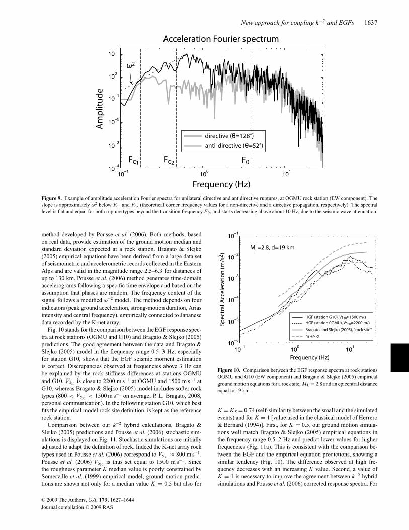
equal to 0.25 s, which is the average value proposed by Somervilleet al. (1999) for a MW 5.5 earthquake. Fig. 8 displays the effectsof the source parameters uncertainties on the ground accelerationand velocity at rock station OGMU. Are also shown examples ofamplitude acceleration Fourier spectra for unilateral directive andantidirective ruptures (Fig. 9).

Simulation on rock and validation

In order to test the reliability of the ground motion predictions,simulations on rock site are compared to the empirical ground mo-tions equations of Bragato & Slejko (2005) and to the stochastic

C© 2009 The Authors, GJI, 179, 1627–1644



Figure 9. Example of amplitude acceleration Fourier spectra for unilateral directive and antidirective ruptures, at OGMU rock station (EW component). Theslope is approximately ω2 below Fc1 and Fc2 (theoretical corner frequency values for a non-directive and a directive propagation, respectively). The spectrallevel is flat and equal for both rupture types beyond the transition frequency F0, and starts decreasing above about 10 Hz, due to the seismic wave attenuation.

method developed by Pousse et al. (2006). Both methods, basedon real data, provide estimation of the ground motion median andstandard deviation expected at a rock station. Bragato & Slejko(2005) empirical equations have been derived from a large data setof seismometric and accelerometric records collected in the EasternAlps and are valid in the magnitude range 2.5–6.3 for distances ofup to 130 km. Pousse et al. (2006) method generates time-domainaccelerograms following a specific time envelope and based on theassumption that phases are random. The frequency content of thesignal follows a modified ω−2 model. The method depends on fourindicators (peak ground acceleration, strong-motion duration, Ariasintensity and central frequency), empirically connected to Japanesedata recorded by the K-net array.

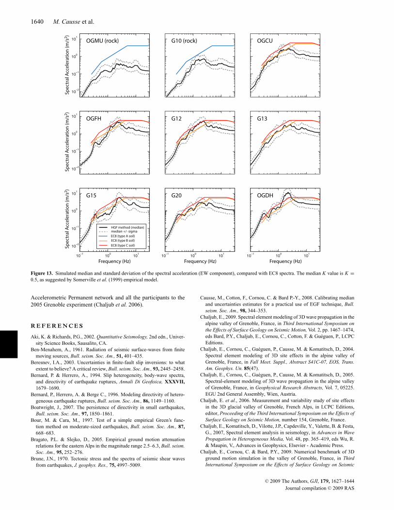
Fig. 10 stands for the comparison between the EGF response spec-tra at rock stations (OGMU and G10) and Bragato & Slejko (2005)predictions. The good agreement between the data and Bragato &Slejko (2005) model in the frequency range 0.5–3 Hz, especiallyfor station G10, shows that the EGF seismic moment estimationis correct. Discrepancies observed at frequencies above 3 Hz canbe explained by the rock stiffness differences at stations OGMUand G10. VS30 is close to 2200 m s−1 at OGMU and 1500 m s−1 atG10, whereas Bragato & Slejko (2005) model includes softer rocktypes (800 < VS30 < 1500 m s−1 on average; P. L. Bragato, 2008,personal communication). In the following station G10, which bestfits the empirical model rock site definition, is kept as the referencerock station.

Comparison between our k−2 hybrid calculations, Bragato &Slejko (2005) predictions and Pousse et al. (2006) stochastic sim-ulations is displayed on Fig. 11. Stochastic simulations are initiallyadjusted to adapt the definition of rock. Indeed the K-net array rocktypes used in Pousse et al. (2006) correspond to VS30 ≈ 800 m s−1.Pousse et al. (2006) VS30 is thus set equal to 1500 m s−1. Sincethe roughness parameter K median value is poorly constrained bySomerville et al. (1999) empirical model, ground motion predic-tions are shown not only for a median value K = 0.5 but also for

Figure 10. Comparison between the EGF response spectra at rock stationsOGMU and G10 (EW component) and Bragato & Slejko (2005) empiricalground motion equations for a rock site, ML = 2.8 and an epicentral distanceequal to 19 km.

K = K S = 0.74 (self-similarity between the small and the simulatedevents) and for K = 1 [value used in the classical model of Herrero& Bernard (1994)]. First, for K = 0.5, our ground motion simula-tions well match Bragato & Slejko (2005) empirical equations inthe frequency range 0.5–2 Hz and predict lower values for higherfrequencies (Fig. 11a). This is consistent with the comparison be-tween the EGF and the empirical equation predictions, showing asimilar tendency (Fig. 10). The difference observed at high fre-quency decreases with an increasing K value. Second, a value ofK = 1 is necessary to improve the agreement between k−2 hybridsimulations and Pousse et al. (2006) corrected response spectra. For

C© 2009 The Authors, GJI, 179, 1627–1644



Figure 11. (a) Comparison between the response spectra obtained from our k−2 hybrid predictions (station G10, EW component), Bragato & Slejko (2005)empirical ground motion equations and Pousse et al. (2006) stochastic simulations, corrected according to Cotton et al. (2006) procedure (VS30 = 1500 m s−1).The dashed line correspond to the plus and minus standard deviation spectra. (b) Example of accelerograms (station G10, EW component) obtained from thek−2 hybrid procedure. Are also shown example of Pousse et al. (2006) corrected stochastic simulations. The six time-series span the median ground motionwithin ±1 SD.

K = 1, the obtained time-series are also similar in terms of ampli-tude and duration (Fig. 11b). Note that below 1 Hz, the stochasticsimulations exceed the other predictions of a factor of about 2.This difference may come from Pousse et al. (2006) procedure,that overestimates the acceleration Fourier amplitude below thecorner frequency for moderate sized earthquakes (Fabian Bonilla,2008, personal communication—see also fig. 8 of Pousse et al.2006).

Despite the discrepancies observed at high frequency, one canconclude that our simulations are consistent with Bragato & Slejko(2005) empirical equations and the stochastic simulations, for thethree tested K values.

Simulation on sediment

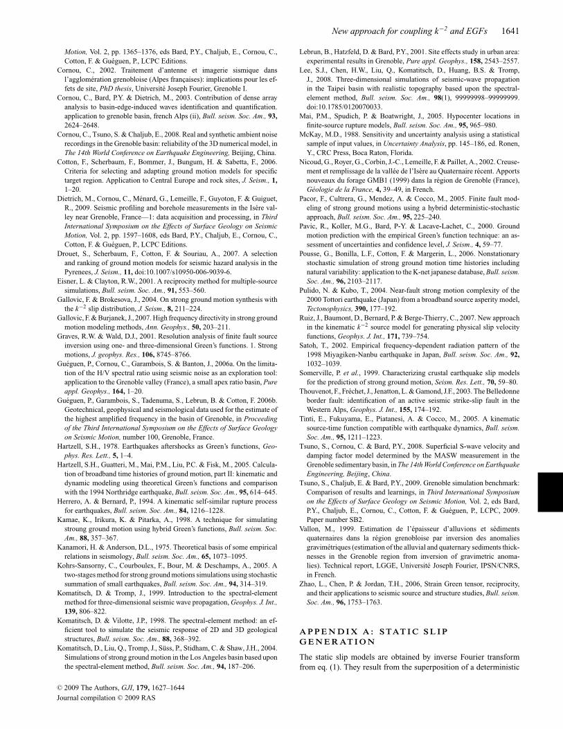
In order to simulate ground motion at sediment stations, a K value of0.5 is kept, since it results from past earthquake analysis (Somervilleet al. 1999, relationships). The comparison at the rock station G10with Bragato & Slejko (2005) empirical equation results and Pousseet al. (2006) corrected simulations suggests that K = 0.5 does notlead to overestimated ground motion. Fig. 12 displays the accelero-grams derived from median source parameter values at the 9 stationsand Fig. 13 displays median and standard deviation of the simulatedresponse spectra. The spectra are compared with the European regu-lation spectra (EC8) for rock site (category A in EC8 classification)

or for standard to stiff soils (category B and C) for the stations lo-cated within the basin. First, our predictions exceed the EC8 spectraat some sites and some frequencies, especially at station OGDH,which exhibits two peaks at 0.3 and 2 Hz. The first peak, gener-ated by 3-D simulations (<1 Hz), corresponds to the fundamentalresonance frequency of the sedimentary basin (Lebrun et al. 2001;Gueguen et al. 2006a). This peak also clearly appears at stationsOGFH, G15 and G20. This confirms the importance of couplingthe EGF with 3-D numerical calculations. The second peak at 2 Hzhas been well identified from geophysical and geotechnical surveys(Gueguen et al. 2006b, P. Gueguen and S. Garambois, unpublishedmanuscript) and from global inversion methods (Drouet et al. 2007).This is interpreted as the resonance effects within a surficial softclay layer overlaying more competent sandy graver layers. Second,the spectral responses at stations G20 and OGDH, located only afew hundreds of meters away, obviously diverge beyond 1 Hz. Thispoints out the large spatial variability of the high-frequency ampli-fication effects, caused by fast lateral variations of the upper softsediment layers (Tsuno et al. 2008). Such variations are observedfrom several drillings and surface wave measurements performedin this area. Third, the EC8 design spectra largely exceed our sim-ulations at rock stations OGMU and G10. These results indicatethat standard European regulations provide a frequency-dependentand site-dependent safety margin in the Grenoble basin. The useof HGFs suggests the need of specific design spectra in Grenoble,

C© 2009 The Authors, GJI, 179, 1627–1644



Figure 12. Simulated accelerograms for median parameter values. The maximum value is indicated on the right of each accelerogram.

with increased low-frequency level in the valley and much smallerspectra on rock. Microzonation studies are thus preferable in sucha specific geological context.

C O N C LU S I O N

A new method has been introduced for performing broad-bandground motion time histories from a finite-extent source model.This method includes specific site effects and is adequate forsimulating ground motion in 3-D deep alluvial valleys. The groundacceleration is computed in the frequency range 0.1–30 Hz witha new approach coupling k−2 source model and HGFs, obtainedby summing reciprocity-based SEM 3-D simulations (<1 Hz) andEGFs. A procedure is proposed to assess the ground motion predic-tion variability due to the source rupture process, from specific dis-tributions of the k−2 model parameters. We used this new approachfor predicting ground motion for a potential MW 5.5 earthquake inthe Grenoble valley. At sediment sites, the simulated response spec-tra significantly differ from one station to the other. At some sitessimulations present large response spectra both at high-frequency(>1 Hz) and low-frequency (≈0.3 Hz) and EC8 spectra are ex-ceeded. This points out the interest of coupling EGFs and 3-Dnumerical simulations in such deep valleys.

The method presented relies on reliable estimation of the sourcemodel parameter distributions. Our ground motion estimations es-pecially depends on the slip distribution roughness, controlled by theparameter K. In order to estimate the a priori K value distribution,Somerville et al. (1999) scaling laws have been used. Neverthe-

less, the reliability of these relationships may be questionable. First,Somerville et al. (1999) results have been derived from a small num-ber of inverted source models (15) and the event magnitudes MW

range from 5.6 to 7.2, which decreases the K estimation robustnessfor a MW 5.5 event. Second, the inverse problem parametrizationoften involves subjective decision resulting in highly different in-verted slip images and there is no basis to distinguish betweenartefacts, smoothing constraints and real features (Beresnev 2003).The comparison made in Fig. 11 indicates that a median K valueof 0.5 may result in underestimated ground motion. There is thus aneed of improving earthquake model databases to better constrainsource parameters for performing blind predictions. An other ap-proach would have been to set the median K value equal to 1, whichleads to the best fit between the predictions at rock station G10,Bragato & Slejko (2005) predictions and Pousse et al. (2006) cor-rected simulations. Such a calibration is also proposed by Causseet al. (2008). Nevertheless, this approach would not change thegeneral conclusion on the comparison between the ground motionpredictions at sediment stations and the EC8 design spectra.

A C K N OW L E D G M E N T S

Mathieu Causse’s grant is funded by CEA and CNRS. Thiswork benefits from ANR-QSHA and SIRSEG(MEDAD) programs.Fabrice Cotton’s work is supported by Institut Universitaire deFrance. All the computations presented in this paper were per-formed at the Service Commun de Calcul Intensif de l’Observatoirede Grenoble (SCCI). The authors would also like to thank the French

C© 2009 The Authors, GJI, 179, 1627–1644



Figure 13. Simulated median and standard deviation of the spectral acceleration (EW component), compared with EC8 spectra. The median K value is K =0.5, as suggested by Somerville et al. (1999) empirical model.

Accelerometric Permanent network and all the participants to the2005 Grenoble experiment (Chaljub et al. 2006).

R E F E R E N C E S

Aki, K. & Richards, P.G., 2002. Quantitative Seismology, 2nd edn., Univer-sity Science Books, Sausalito, CA.

Ben-Menahem, A., 1961. Radiation of seismic surface-waves from finitemoving sources, Bull. seism. Soc. Am., 51, 401–435.

Beresnev, I.A., 2003. Uncertainties in finite-fault slip inversions: to whatextent to believe? A critical review, Bull. seism. Soc. Am., 93, 2445–2458.

Bernard, P. & Herrero, A., 1994. Slip heterogeneity, body-wave spectra,and directivity of earthquake ruptures, Annali Di Geofisica, XXXVII,1679–1690.

Bernard, P., Herrero, A. & Berge C., 1996. Modeling directivity of hetero-geneous earthquake ruptures, Bull. seism. Soc. Am., 86, 1149–1160.

Boatwright, J., 2007. The persistence of directivity in small earthquakes,Bull. seism. Soc. Am., 97, 1850–1861.

Bour, M. & Cara, M., 1997. Test of a simple empirical Green’s func-tion method on moderate-sized earthquakes, Bull. seism. Soc. Am., 87,668–683.

Bragato, P.L. & Slejko, D., 2005. Empirical ground motion attenuationrelations for the eastern Alps in the magnitude range 2.5–6.3, Bull. seism.Soc. Am., 95, 252–276.

Brune, J.N., 1970. Tectonic stress and the spectra of seismic shear wavesfrom earthquakes, J. geophys. Res., 75, 4997–5009.

Causse, M., Cotton, F., Cornou, C. & Bard P.-Y., 2008. Calibrating medianand uncertainties estimates for a practical use of EGF technique, Bull.seism. Soc. Am., 98, 344–353.

Chaljub, E., 2009. Spectral element modeling of 3D wave propagation in thealpine valley of Grenoble, France, in Third International Symposium onthe Effects of Surface Geology on Seismic Motion, Vol. 2, pp. 1467–1474,eds Bard, P.Y., Chaljub, E., Cornou, C., Cotton, F. & Gueguen, P., LCPCEditions.

Chaljub, E., Cornou, C., Gueguen, P., Causse, M. & Komatitsch, D., 2004.Spectral element modeling of 3D site effects in the alpine valley ofGrenoble, France, in Fall Meet. Suppl., Abstract S41C-07, EOS, Trans.Am. Geophys. Un. 85(47).

Chaljub, E., Cornou, C., Gueguen, P., Causse, M. & Komatitsch, D., 2005.Spectral-element modeling of 3D wave propagation in the alpine valleyof Grenoble, France, in Geophysical Research Abstracts, Vol. 7, 05225.EGU 2nd General Assembly, Wien, Austria.

Chaljub, E. et al., 2006. Measurement and variability study of site effectsin the 3D glacial valley of Grenoble, French Alps, in LCPC Editions,editor, Proceeding of the Third International Symposium on the Effects ofSurface Geology on Seismic Motion, number 154, Grenoble, France.

Chaljub, E., Komatitsch, D., Vilotte, J.P., Capdeville, Y., Valette, B. & Festa,G., 2007, Spectral element analysis in seismology, in Advances in WavePropagation in Heterogeneous Media, Vol. 48, pp. 365–419, eds Wu, R.& Maupin, V., Advances in Geophysics, Elsevier - Academic Press.

Chaljub, E., Cornou, C. & Bard, P.Y., 2009. Numerical benchmark of 3Dground motion simulation in the valley of Grenoble, France, in ThirdInternational Symposium on the Effects of Surface Geology on Seismic

C© 2009 The Authors, GJI, 179, 1627–1644



Motion, Vol. 2, pp. 1365–1376, eds Bard, P.Y., Chaljub, E., Cornou, C.,Cotton, F. & Gueguen, P., LCPC Editions.

Cornou, C., 2002. Traitement d’antenne et imagerie sismique dansl’agglomeration grenobloise (Alpes francaises): implications pour les ef-fets de site, PhD thesis, Universite Joseph Fourier, Grenoble I.

Cornou, C., Bard, P.Y. & Dietrich, M., 2003. Contribution of dense arrayanalysis to basin-edge-induced waves identification and quantification.application to grenoble basin, french Alps (ii), Bull. seism. Soc. Am., 93,2624–2648.

Cornou, C., Tsuno, S. & Chaljub, E., 2008. Real and synthetic ambient noiserecordings in the Grenoble basin: reliability of the 3D numerical model, inThe 14th World Conference on Earthquake Engineering, Beijing, China.

Cotton, F., Scherbaum, F., Bommer, J., Bungum, H. & Sabetta, F., 2006.Criteria for selecting and adapting ground motion models for specifictarget region. Application to Central Europe and rock sites, J. Seism., 1,1–20.

Dietrich, M., Cornou, C., Menard, G., Lemeille, F., Guyoton, F. & Guiguet,R., 2009. Seismic profiling and borehole measurements in the Isere val-ley near Grenoble, France—1: data acquisition and processing, in ThirdInternational Symposium on the Effects of Surface Geology on SeismicMotion, Vol. 2, pp. 1597–1608, eds Bard, P.Y., Chaljub, E., Cornou, C.,Cotton, F. & Gueguen, P., LCPC Editions.

Drouet, S., Scherbaum, F., Cotton, F. & Souriau, A., 2007. A selectionand ranking of ground motion models for seismic hazard analysis in thePyrenees, J. Seism., 11, doi:10.1007/s10950-006-9039-6.

Eisner, L. & Clayton, R.W., 2001. A reciprocity method for multiple-sourcesimulations, Bull. seism. Soc. Am., 91, 553–560.

Gallovic, F. & Brokesova, J., 2004. On strong ground motion synthesis withthe k−2 slip distribution, J. Seism., 8, 211–224.

Gallovic, F. & Burjanek, J., 2007. High frequency directivity in strong groundmotion modeling methods, Ann. Geophys., 50, 203–211.

Graves, R.W. & Wald, D.J., 2001. Resolution analysis of finite fault sourceinversion using one- and three-dimensional Green’s functions. 1. Strongmotions, J. geophys. Res., 106, 8745–8766.

Gueguen, P., Cornou, C., Garambois, S. & Banton, J., 2006a. On the limita-tion of the H/V spectral ratio using seismic noise as an exploration tool:application to the Grenoble valley (France), a small apex ratio basin, Pureappl. Geophys., 164, 1–20.

Gueguen, P., Garambois, S., Tadenuma, S., Lebrun, B. & Cotton, F. 2006b.Geotechnical, geophysical and seismological data used for the estimate ofthe highest amplified frequency in the basin of Grenoble, in Proceedingof the Third International Symposium on the Effects of Surface Geologyon Seismic Motion, number 100, Grenoble, France.

Hartzell, S.H., 1978. Earthquakes aftershocks as Green’s functions, Geo-phys. Res. Lett., 5, 1–4.

Hartzell, S.H., Guatteri, M., Mai, P.M., Liu, P.C. & Fisk, M., 2005. Calcula-tion of broadband time histories of ground motion, part II: kinematic anddynamic modeling using theoretical Green’s functions and comparisonwith the 1994 Northridge earthquake, Bull. seism. Soc. Am., 95, 614–645.

Herrero, A. & Bernard, P., 1994. A kinematic self-similar rupture processfor earthquakes, Bull. seism. Soc. Am., 84, 1216–1228.

Kamae, K., Irikura, K. & Pitarka, A., 1998. A technique for simulatingstroung ground motion using hybrid Green’s functions, Bull. seism. Soc.Am., 88, 357–367.

Kanamori, H. & Anderson, D.L., 1975. Theoretical basis of some empiricalrelations in seismology, Bull. seism. Soc. Am., 65, 1073–1095.

Kohrs-Sansorny, C., Courboulex, F., Bour, M. & Deschamps, A., 2005. Atwo-stages method for strong ground motions simulations using stochasticsummation of small earthquakes, Bull. seism. Soc. Am., 94, 314–319.

Komatitsch, D. & Tromp, J., 1999. Introduction to the spectral-elementmethod for three-dimensional seismic wave propagation, Geophys. J. Int.,139, 806–822.

Komatitsch, D. & Vilotte, J.P., 1998. The spectral-element method: an ef-ficient tool to simulate the seismic response of 2D and 3D geologicalstructures, Bull. seism. Soc. Am., 88, 368–392.

Komatitsch, D., Liu, Q., Tromp, J., Suss, P., Stidham, C. & Shaw, J.H., 2004.Simulations of strong ground motion in the Los Angeles basin based uponthe spectral-element method, Bull. seism. Soc. Am., 94, 187–206.

Lebrun, B., Hatzfeld, D. & Bard, P.Y., 2001. Site effects study in urban area:experimental results in Grenoble, Pure appl. Geophys., 158, 2543–2557.

Lee, S.J., Chen, H.W., Liu, Q., Komatitsch, D., Huang, B.S. & Tromp,J., 2008. Three-dimensional simulations of seismic-wave propagationin the Taipei basin with realistic topography based upon the spectral-element method, Bull. seism. Soc. Am., 98(1), 99999998–99999999.doi:10.1785/0120070033.

Mai, P.M., Spudich, P. & Boatwright, J., 2005. Hypocenter locations infinite-source rupture models, Bull. seism. Soc. Am., 95, 965–980.

McKay, M.D., 1988. Sensitivity and uncertainty analysis using a statisticalsample of input values, in Uncertainty Analysis, pp. 145–186, ed. Ronen,Y., CRC Press, Boca Raton, Florida.

Nicoud, G., Royer, G., Corbin, J.-C., Lemeille, F. & Paillet, A., 2002. Creuse-ment et remplissage de la vallee de l’Isere au Quaternaire recent. Apportsnouveaux du forage GMB1 (1999) dans la region de Grenoble (France),Geologie de la France, 4, 39–49, in French.

Pacor, F., Cultrera, G., Mendez, A. & Cocco, M., 2005. Finite fault mod-eling of strong ground motions using a hybrid deterministic-stochasticapproach, Bull. seism. Soc. Am., 95, 225–240.

Pavic, R., Koller, M.G., Bard, P-Y. & Lacave-Lachet, C., 2000. Groundmotion prediction with the empirical Green’s function technique: an as-sessment of uncertainties and confidence level, J. Seism., 4, 59–77.

Pousse, G., Bonilla, L.F., Cotton, F. & Margerin, L., 2006. Nonstationarystochastic simulation of strong ground motion time histories includingnatural variability: application to the K-net japanese database, Bull. seism.Soc. Am., 96, 2103–2117.

Pulido, N. & Kubo, T., 2004. Near-fault strong motion complexity of the2000 Tottori earthquake (Japan) from a broadband source asperity model,Tectonophysics, 390, 177–192.

Ruiz, J., Baumont, D., Bernard, P. & Berge-Thierry, C., 2007. New approachin the kinematic k−2 source model for generating physical slip velocityfunctions, Geophys. J. Int., 171, 739–754.

Satoh, T., 2002. Empirical frequency-dependent radiation pattern of the1998 Miyagiken-Nanbu earthquake in Japan, Bull. seism. Soc. Am., 92,1032–1039.

Somerville, P. et al., 1999. Characterizing crustal earthquake slip modelsfor the prediction of strong ground motion, Seism. Res. Lett., 70, 59–80.

Thouvenot, F., Frechet, J., Jenatton, L. & Gamond, J.F., 2003. The Belledonneborder fault: identification of an active seismic strike-slip fault in theWestern Alps, Geophys. J. Int., 155, 174–192.

Tinti, E., Fukuyama, E., Piatanesi, A. & Cocco, M., 2005. A kinematicsource-time function compatible with earthquake dynamics, Bull. seism.Soc. Am., 95, 1211–1223.

Tsuno, S., Cornou, C. & Bard, P.Y., 2008. Superficial S-wave velocity anddamping factor model determined by the MASW measurement in theGrenoble sedimentary basin, in The 14th World Conference on EarthquakeEngineering, Beijing, China.

Tsuno, S., Chaljub, E. & Bard, P.Y., 2009. Grenoble simulation benchmark:Comparison of results and learnings, in Third International Symposiumon the Effects of Surface Geology on Seismic Motion, Vol. 2, eds Bard,P.Y., Chaljub, E., Cornou, C., Cotton, F. & Gueguen, P., LCPC, 2009.Paper number SB2.

Vallon, M., 1999. Estimation de l’epaisseur d’alluvions et sedimentsquaternaires dans la region grenobloise par inversion des anomaliesgravimetriques (estimation of the alluvial and quaternary sediments thick-nesses in the Grenoble region from inversion of gravimetric anoma-lies). Technical report, LGGE, Universite Joseph Fourier, IPSN/CNRS,in French.

Zhao, L., Chen, P. & Jordan, T.H., 2006, Strain Green tensor, reciprocity,and their applications to seismic source and structure studies, Bull. seism.Soc. Am., 96, 1753–1763.

A P P E N D I X A : S TAT I C S L I PG E N E R AT I O N

The static slip models are obtained by inverse Fourier transformfrom eq. (1). They result from the superposition of a deterministic

C© 2009 The Authors, GJI, 179, 1627–1644



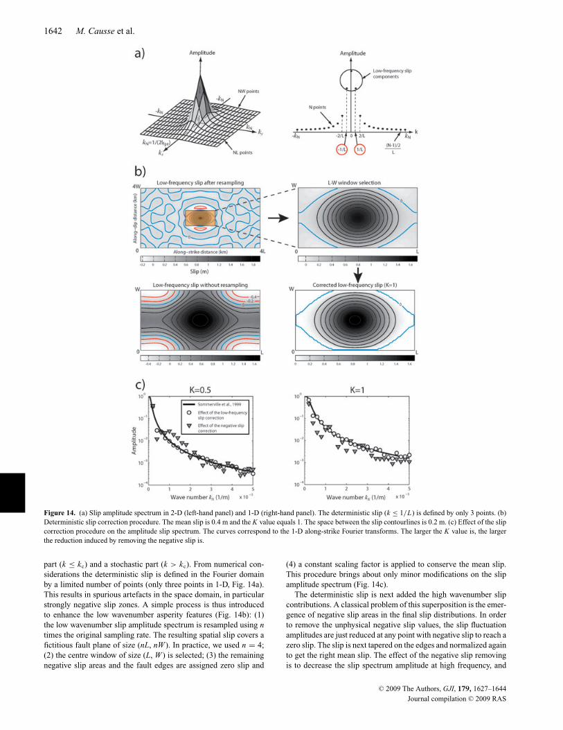
Figure 14. (a) Slip amplitude spectrum in 2-D (left-hand panel) and 1-D (right-hand panel). The deterministic slip (k ≤ 1/L) is defined by only 3 points. (b)Deterministic slip correction procedure. The mean slip is 0.4 m and the K value equals 1. The space between the slip contourlines is 0.2 m. (c) Effect of the slipcorrection procedure on the amplitude slip spectrum. The curves correspond to the 1-D along-strike Fourier transforms. The larger the K value is, the largerthe reduction induced by removing the negative slip is.

part (k ≤ kc) and a stochastic part (k > kc). From numerical con-siderations the deterministic slip is defined in the Fourier domainby a limited number of points (only three points in 1-D, Fig. 14a).This results in spurious artefacts in the space domain, in particularstrongly negative slip zones. A simple process is thus introducedto enhance the low wavenumber asperity features (Fig. 14b): (1)the low wavenumber slip amplitude spectrum is resampled using ntimes the original sampling rate. The resulting spatial slip covers afictitious fault plane of size (nL, nW ). In practice, we used n = 4;(2) the centre window of size (L, W ) is selected; (3) the remainingnegative slip areas and the fault edges are assigned zero slip and

(4) a constant scaling factor is applied to conserve the mean slip.This procedure brings about only minor modifications on the slipamplitude spectrum (Fig. 14c).

The deterministic slip is next added the high wavenumber slipcontributions. A classical problem of this superposition is the emer-gence of negative slip areas in the final slip distributions. In orderto remove the unphysical negative slip values, the slip fluctuationamplitudes are just reduced at any point with negative slip to reach azero slip. The slip is next tapered on the edges and normalized againto get the right mean slip. The effect of the negative slip removingis to decrease the slip spectrum amplitude at high frequency, and

C© 2009 The Authors, GJI, 179, 1627–1644



consequently the source energy. However, this reduction remainsweak for K ≤ 1 because most of the slip is positive (Fig. 14c). Be-sides our tests show that the apparent source time function spectraldecay is preserved and that the high-frequency energy decrease isalso weak for K ≤ 1 (cf. Section ‘Summation Algorithm’, Fig. 4e).For simulating with higher K values, negative slip values can bekept but the k−2 source model has to be considered as a purelymathematical tool providing the expected source spectrum charac-teristics.

A P P E N D I X B : C A L C U L AT I O N O FT H E T H E O R E T I C A L A S T F H I G H -F R E Q U E N C Y S P E C T R A L L E V E L

From eq. (11), the ASTF amplitude spectrum is such that:

|R( f )| = |U ( f )|/|u( f )|, (B1)

where U ( f ) and u( f ) denotes the simulated event and the EGF dis-placement spectra, respectively. Beyond the EGF corner frequencyf c, both events have a ω−2 spectral decay. Hence the theoreticalASTF amplitude spectrum is a plateau, the level of which is:

|R( f ≥ fc)|theo = |U ( fc)|theo/|u( fc)|theo. (B2)

The theoretical displacement spectrum amplitude of the targetevent at frequency f c is

|U ( fc)|theo = Ao

4π 2 f 2c

. (B3)

The Ao value is given by eq. (5) and the corner frequency of thesmall event, that is assumed to follow a k−2 model, is such that:fc = vKS

l , with K S ≈ 0.74 (eq. 8).Besides, the propagation effects and radiation patterns and sup-

posed to be the same for both EGF and simulated event. It leadsto:

|u( fc)|theo = Csmo, (B4)

After eqs (B2), (B3) and (B4), and by assuming that both eventshave the same rupture velocity, we obtain

|R( f ≥ fc)|theo = RMS[Cd (�)2 X (Cd (�)/2)

] (Mo

mo

)(l

L

)2( K

KS

)2

.

(B5)

For a ratio v/c = 0.8 and for a Gaussian slip velocity function witha standard deviation σ = τ/10 RMS[Cd(�)2 X (Cd(�)/2)] ≈ 1.9.Thus, eq. (B5) gives

|R( fc)|theo = βN K 2, (B6)

with β ≈ 3.5.

A P P E N D I X C : C A L C U L AT I O NO F T H E E G F N U M B E R T O S U MF O R T H E H I G H - F R E Q U E N C YA S T F L E V E L C O R R E C T I O N

In order to obtain the expected level |R( f ≥ f c)|theo, the averagenumber of EGFs to sum along the rise time dislocation is adapted.This choice comes to assume a new EGF dislocation. Let d/γ be themodified EGF dislocation. At low frequency, the EGF summing upis coherent. Hence the ASTF amplitude becomes γ N 3. To conserve

Figure 15. Representation of the slip distribution Dk (x , y) for a givenwavenumber k. The integrals I1 and I2 (eqs 26 and 27) represents theintegrals of |Dk (x , y)| over the surfaces S1 and S2, respectively.

the seismic moment, the whole spectrum is divided by γ . Besides,beyond f c, the summation is incoherent. Therefore, the ASTF levelbecomes the square root of the EGF quadratic sum, each EGF beingrepresented by a Dirac function with amplitude 1 or −1. This leadsto

|R( f ≥ fc)|obs = 1

γ

√γ (NSTO + NDET), (C1)

where N DET = N 3 and N STO is the total number of summed EGFresulting from the stochastic slip heterogeneities. The deterministicslip contribution to the ASTF is low-pass filtered to keep only thestochastic slip contributions beyond f c. Thus, eq. (C1) gives

|R( f ≥ fc)|obs =(

NSTO

γ

)1/2

. (C2)

N STO calculation

In order to estimate N STO, the surface slip density for a givenwavenumber k > 1/

√L2 + W 2 is calculated. It is defined as

ρsk = 1

LW

∫ L

0

∫ W

0|Dk(x, y)|dxdy, (C3)

where Dk(x , y) represents the slip distribution for the wavenumberk. Using the integrals I1 and I2 of |Dk(x , y)| over the surfaces S1

and S2, respectively (Fig. 15), we obtain

ρsk = 1

LW· 2(I1 + I2) · 2Lkx · 2W ky

= 8kx ky(I1 + I2), (C4)

with

I1 = 2Dk(kx , ky)∫ 1

4kx

0

∫ 14ky

0

∣∣sin[2π (kx x + ky y)]∣∣ dxdy

= Dk(kx , ky)

π 2kx ky

(C5)

and

I2 = 2Dk(kx , ky)∫ 1

4ky

0

∫ 14ky

− kykx

0

∣∣cos[2π (kx x + ky y)]∣∣ dxdy

= (π − 2)

2

Dk(kx , ky)

π 2kx ky. (C6)

C© 2009 The Authors, GJI, 179, 1627–1644



It leads to

ρsk = 4Dk(kx , ky)

π. (C7)

The overall surfacic slip density ρs is obtain by summing all thehigh wavenumber contributions

ρs = 2∫ kxmax

kxmin

∫ kymax

kymin

ρsk dkx dky . (C8)

From eq. (1) we come to

ρs ≈ 8

πDK 2

∫ kxmax

kxmin

∫ kymax

kymin

1

k2x + k2

y

dkx dky . (C9)

In the following a square fault plane is assumed (L = W ).Hence from numerical considerations (see Appendix A, Fig. 14a):kxmin = kymin = 2

l(N−1) and kxmax = kymax = kN = 12l . Next cartesian

coordinates are replaced with polar coordinates (r , �) in eq. (C9).It leads to the following approximation:

ρs ≈ 8

πDK 2

∫ π/2

0

∫ 12l

2l(N−1)

1

r 2 cos �2 + r 2 sin �2rdrd�

≈ 4DK 2 ln

(N − 1

4

). (C10)

Besides N STO is related to ρs according to

NSTO = ρs L2

dl2. (C11)

Then, inserting (C10) into (C11) we get

NSTO ≈ α(N )2 N 3 K 2, (C12)

with α(N ) = 2√

ln(

N−14

).

� Calculation of the adapted EGF dislocation d/γ

After eqs (C2) and (C12), the observed ATSF spectral level is:

|R( f ≥ fc)|obs = α(N )

γ 1/2N 3/2 K . (C13)

Finally, after eq. (B6), the condition: |R( f ≥ f c)|obs = |R( f c)|theo

leads to

α(N )

γ 1/2N 3/2 K = βN K 2. (C14)

Consequently, the new EGF dislocation to be considered is d/γ

with

γ =(

α(N )

β

)2 N

K 2, (C15)

where α(N ) = 2√

ln(

N−14

)and β ≈ 3.5.

C© 2009 The Authors, GJI, 179, 1627–1644


Geophysical Journal International - ISTerre de G´eophysique Interne et de Tectonophysique (LGIT),...

Documents

Transcript of Geophysical Journal International - ISTerre de G´eophysique Interne et de Tectonophysique (LGIT),...